1
Machine Model Parameter
Determination
User Manual
May07-18
Client:
General Electric
Faculty Advisor:
Chen-Ching Liu
Team Members:
Jared Kline
Adam Wroblaski
Mark Reisinger
Yu Chan
Disclaimer
This document was developed as a part of the requirements of an electrical and
computer engineering course at Iowa State University, Ames, Iowa. This document
does not constitute a professional engineering design or a professional land surveying
document. Although the information is intended to be accurate, the associated
students, faculty, and Iowa State University make no claims, promises, or guarantees
about the accuracy, completeness, quality, or adequacy of the information. The user
of this document shall ensure that any such use does not violate any laws with regard
to professional licensing and certification requirements. This use includes any work
resulting from this student-prepared document that is required to be under the
responsible charge of a licensed engineer or surveyor. This document is copyrighted
by the students who produced this document and the associated faculty advisors. No
part may be reproduced without the written permission of the senior design course
coordinator.
Submitted
April 24, 2007
May07-18
User Manual
4/24/2007
Table of Contents
1
INTRODUCTION.......................................................................................................................... 1
1.1
PURPOSE AND INTENDED USE OF THIS MANUAL ........................................................................... 1
1.2
ACKNOWLEDGMENTS ................................................................................................................... 1
2
BASIC USE..................................................................................................................................... 2
2.1
STARTING PROGRAM .................................................................................................................... 2
2.2
ADJUSTING PARAMETERS ............................................................................................................ 5
2.3
SELECTING A TEST ....................................................................................................................... 6
2.4
RUNNING SIMULATIONS ............................................................................................................... 6
2.5
RUNNING BATCH SIMULATIONS ................................................................................................... 6
2.6
LOADING TEST DATA ................................................................................................................... 7
2.7
SAVING AND LOADING PARAMETERS ........................................................................................... 8
2.8
SAVING GRAPHS AND EXPORTING SIMULATION DATA .............................................................. 10
3
PROGRAM STRUCTURE ......................................................................................................... 13
3.1
DESIGN OVERVIEW .................................................................................................................... 13
3.1.1
Program Components........................................................................................................... 13
3.1.1.1
Basic Algorithm ............................................................................................................... 14
3.1.1.2
Graphical User Interface................................................................................................. 15
3.1.1.3
Simulink Models............................................................................................................... 15
3.1.1.4
Simulation Scripts ............................................................................................................ 16
3.1.2
The Matlab Workspace ......................................................................................................... 16
3.1.3
Setting Files .......................................................................................................................... 16
3.1.4
Test Data .............................................................................................................................. 16
3.1.5
Interaction Between Components and Flow of Information ................................................. 17
3.2
GRAPHICAL USER INTERFACE .................................................................................................... 18
3.2.1
Data Structures..................................................................................................................... 18
3.2.2
Opening Window .................................................................................................................. 20
3.2.2.1
Structure..................................................................................................................................... 21
3.2.2.2
Main Window Setting File ......................................................................................................... 21
3.2.3
Home Window....................................................................................................................... 22
3.2.3.1
Structure..................................................................................................................................... 23
3.2.3.1.1
Features................................................................................................................................. 24
3.2.3.1.2
Callback Functions ............................................................................................................... 25
3.2.3.1.2.1
Slider Bar and Edit Box Callback Functions .................................................................. 25
3.2.3.1.2.2
Test Selection Menu Callback Function ......................................................................... 26
3.2.3.1.2.3
Simulate Button Callback Function................................................................................ 26
May07-18
Introduction
Page 1 of 5
May07-18
4/24/2007
3.2.3.1.2.4
Batch Simulate Button Callback Function...................................................................... 26
3.2.3.1.2.5
Open Button Callback Function ..................................................................................... 27
3.2.3.1.2.6
Save Button Callback Function ...................................................................................... 28
3.2.3.1.2.7
Undo/Redo Button Callback Functions .......................................................................... 29
3.2.3.1.2.8
Zoom In, Zoom Out, and Pan Button Callback Functions.............................................. 29
3.2.3.2
3.2.4
User Manual
GUI Setting File......................................................................................................................... 30
Batch Simulation Window..................................................................................................... 30
3.3
SIMULATION SCRIPTS ................................................................................................................. 30
3.4
SIMULINK MODEL ...................................................................................................................... 31
4
PROGRAM MAINTENANCE ................................................................................................... 32
4.1
ADDING MODELS TO LIBRARY ................................................................................................... 32
4.1.1
Compatible Simulink Models................................................................................................ 32
4.1.2
Compatible Simulation Scripts ............................................................................................. 32
4.1.3
Creating GUI Setting File .................................................................................................... 33
4.1.4
Editing Main Window Setting File........................................................................................ 33
4.1.5
Example: Creation and Addition of Classical Machine vs. Infinite Bus............................... 34
4.1.5.1
Preparation ................................................................................................................................. 34
4.1.5.2
Creation of Simulink Model....................................................................................................... 36
4.1.5.3
Creation of Simulation Script..................................................................................................... 43
4.1.5.4
Creation of GUI Setting File ...................................................................................................... 50
4.1.5.5
Modification of Main Window Setting File ............................................................................... 56
4.1.5.6
Final Simulation Script Modifications ....................................................................................... 57
4.2
TESTING LIBRARY ADDITIONS ................................................................................................... 60
4.3
TROUBLESHOOTING LIBRARY ADDITIONS.................................................................................. 60
4.3.1
Errors in Main Window Setting File..................................................................................... 61
4.3.2
Errors in GUI Setting File.................................................................................................... 61
4.3.3
Errors in Simulation Script................................................................................................... 62
4.3.4
Errors in Simulink Block Diagram ....................................................................................... 62
APPENDIX A DETAILED FLOW CHART...................................................................................... 63
APPENDIX B SAMPLE TEST DATA ............................................................................................... 64
APPENDIX C SAMPLE GUI SETTING FILE................................................................................. 65
APPENDIX D SAMPLE SIMULINK BLOCK DIAGRAM............................................................. 68
APPENDIX E SAMPLE SIMULATION SCRIPT............................................................................ 69
May07-18
Introduction
Page 2 of 5
May07-18
User Manual
4/24/2007
List of Figures
FIGURE 2.1 CHANGING MATLAB DIRECTORY ................................................................................................. 2
FIGURE 2.2 RUNNING MAIN_WINDOW.M ......................................................................................................... 3
FIGURE 2.3 OPENING WINDOW ....................................................................................................................... 4
FIGURE 2.4 HOME SCREEN .............................................................................................................................. 5
FIGURE 2.5 SLIDER BAR .................................................................................................................................. 5
FIGURE 2.6 TEST PULL DOWN MENU .............................................................................................................. 6
FIGURE 2.7 SIMULATE AND BATCH SIMULATE BUTTONS ................................................................................ 6
FIGURE 2.8 BATCH SIMULATION WINDOW ...................................................................................................... 7
FIGURE 2.9 LOADING TEST DATA ................................................................................................................... 8
FIGURE 2.10 SAVING PARAMETERS ................................................................................................................. 9
FIGURE 2.11 OPENING SAVED PARAMETER SETTINGS .................................................................................. 10
FIGURE 2.12 SAVING GRAPHS ....................................................................................................................... 11
FIGURE 2.13 EXPORTING SIMULATION DATA ................................................................................................ 12
FIGURE 3.1 SIMPLIFIED FLOW OF INFORMATION ........................................................................................... 14
FIGURE 3.2 SIMPLIFIED FLOW CHART ........................................................................................................... 15
FIGURE 3.3 DETAILED FLOW OF INFORMATION ............................................................................................. 17
FIGURE 3.4 OPENING WINDOW..................................................................................................................... 20
FIGURE 3.5 HOME WINDOW .......................................................................................................................... 22
FIGURE 3.6 WAIT BAR ................................................................................................................................... 24
FIGURE 3.7 SIMULATION ERROR MESSAGE BOX ........................................................................................... 26
FIGURE 3.8 BATCH SIMULATE WINDOW ....................................................................................................... 27
FIGURE 3.9 OPEN WINDOW ........................................................................................................................... 28
FIGURE 3.10 SAVE AS WINDOW .................................................................................................................... 29
FIGURE 4.1 BLOCK DIAGRAM OF CLASSICAL MODEL ................................................................................... 35
FIGURE 4.2 BASIC BLOCK DIAGRAM AS SIMULINK MODEL .......................................................................... 37
FIGURE 4.3 INTEGRAL INITIAL CONDITION.................................................................................................... 38
FIGURE 4.4 IMBEDDED MATLAB FUNCTION .................................................................................................. 39
FIGURE 4.5 CLASSICAL MODEL WITH EMBEDDED MATLAB FUNCTION ........................................................ 40
FIGURE 4.6 TO WORKSPACE SETTINGS ......................................................................................................... 41
FIGURE 4.7 COMPLETED CLASSICAL MODEL ................................................................................................ 42
FIGURE 4.8 CONFIGURATION PARAMETERS................................................................................................... 43
FIGURE 4.9 SIMULATION RESULTS ................................................................................................................ 50
May07-18
Introduction
Page 3 of 5
May07-18
User Manual
4/24/2007
List of Tables
TABLE 3.1 SAMPLE TEST DATA FORMAT ...................................................................................................... 17
TABLE 3.2 DATA STRUCTURES AND THEIR FIELDS ........................................................................................ 19
TABLE 3.3 PRODUCT REQUIREMENTS AND FEATURES .................................................................................. 24
TABLE 4.1 GUI PARAMETERS ....................................................................................................................... 36
May07-18
Introduction
Page 4 of 5
May07-18
User Manual
4/24/2007
List of Definitions
•
Block diagram – A visual method commonly used in engineering to depict the
relationship between inputs and outputs of a system.
•
GUIDE – Graphical User Interface Development Environment – A Matlab toolbox
that supplies a graphical and interactive method for the creation of graphical user
interfaces.
•
Initial Conditions – Values that determine the simulation’s starting point.
•
Matlab – A software package developed by Mathworks that is commonly used for
engineering computation.
•
Matlab Workspace – The location where all variables are stored.
•
Physical test results – These are the results of actual generator performance as
physical measured in the field.
•
PSLF – (Positive Sequence Load Flow) – A software tool manufactured by
General Electric that is used by power systems engineers to analyze the
performance and security of large interconnected power systems.
•
PSLF test results – These are the results of control simulations run using PSLF.
•
Semi-real time – Result updates appear after the user selects the run command.
•
Simulink – A Matlab toolbox that allows users to build and analyze block
diagrams.
•
Simulink test results – These are the results obtained using the group created
Simulink tool.
Simulink and Matlab are copyrighted by The Mathworks Inc.
Windows is copyrighted by Microsoft Corporation
PSLF is copyrighted by General Electric Company
May07-18
Introduction
Page 5 of 5
May07-18
User Manual
4/24/2007
1 Introduction
This software was developed by a team of students at Iowa State University and
engineers in the Infrastructure business unit of General Electric. It is intended to assist
engineers in more quickly determining accurate model parameters for use in computer
simulations. It was developed for use in the power industry, specifically the
parameters associated with synchronous machine modeling, but has a variety of
possible applications.
1.1
Purpose and Intended use of this Manual
This document is intended to be used as a guide both to both the use and maintenance
of the software. It includes instructions on the basic use, provides a detailed and
technical overview of the program structure, instructions for adding models to the
library, detailed examples of adding models to the library, and the source code. It is
assumed that the reader is very familiar with Matlab.
1.2
Acknowledgments
The project team would like to thank Doug Welsh, Juan Sanchez and Dan Leonard of
General Electric and Dr. Chen-Ching Liu of Iowa State University for the assistance
and technical expertise that they have provided.
May07-18
Introduction
Page 1 of 73
May07-18
User Manual
4/24/2007
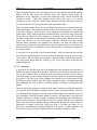
2 Basic Use
This section provides instructions for the basic use of the software including, initial
execution, running both normal and batch simulations, loading test data, saving and
loading parameters, and exporting graphs and simulation data.
2.1
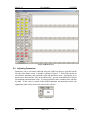
Starting Program
To start the program, open Matlab and change the Matlab directory to the directory
directory containing the program files. This is shown in Figure 2.1.
Figure 2.1 Changing Matlab Directory
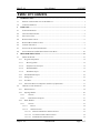
In the current directory portion of the Matlab window, select main_window.m and
right click. Select “Run.” This is shown in Figure 2.2.
May07-18
Basic Use
Page 2 of 73
May07-18
User Manual
4/24/2007
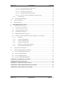
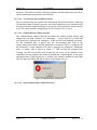
Figure 2.2 Running main_window.m
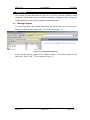
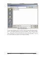
The opening window will appear. A list of all of the models currently in the library
will be in the center select a model and press “Open.” This is shown in Figure 2.3.
May07-18
Basic Use
Page 3 of 73
May07-18
User Manual
4/24/2007
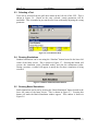
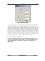
Figure 2.3 Opening Window
After selecting a model and pressing the Open button, the home screen will appear.
This is shown in Figure 2.4.
May07-18
Basic Use
Page 4 of 73
May07-18
User Manual
4/24/2007
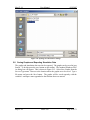
Figure 2.4 Home Screen
2.2
Adjusting Parameters
Parameters can be conviently adjusted using the slider bars that are provided on the
left side of the home screen. A sample is shown in Figure 2.5. Each slider bar has its
own default, minimum, and maximum value and maximum value. Pressing the up or
down arrows increases the value in the edit box by 1 percent of the difference between
the minimum and maximum value. It is also possible to enter a number in the edit box
by hand. If this value is outside of the default minimum and maximum values, the
appropriate limit will be reset to the value in the edit box.
Figure 2.5 Slider Bar
May07-18
Basic Use
Page 5 of 73
May07-18
2.3
User Manual
4/24/2007
Selecting a Test
Tests can be selected from the pull down menu on the left side of the GUI. This is
shown in Figure 2.6. Based on the entry selected, certain parameters will be
uneditable. This is intended to prevent the user from accidentally adjusting the wrong
parameter.
Figure 2.6 Test Pull Down Menu
2.4
Running Simulations
Standard simulations can be run using the “Simulate” button located in the lower left
corner of the home screen. This is shown in Figure 2.7. Pressing this button will
execute the simulation script, Simulink model, and plot the simulations results.
During execution, a waitbar will appear to notify the user that a simulation is being
executed.
Figure 2.7 Simulate and Batch Simulate Buttons
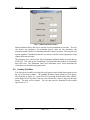
2.5
Running Batch Simulations
Batch simulations can be run by pressing the “Batch Simulation” button located in the
lower left corner of the home screen. This is shown in Figure 2.7. Pressing this
button will make the Batch Simulation window appear. This window is shown in
Figure 2.8.
May07-18
Basic Use
Page 6 of 73
May07-18
User Manual
4/24/2007
Figure 2.8 Batch Simulation Window
Batch simulation allows the user to execute several simulations at one time. The user
can choose one parameter, the minimum logical value for this parameter, the
maximum and the number of simulations that he wishes to perform. The program will
run the number of simulations that the user selects with the selected parameter being
slightly different each time.
The parameter to be varied can be selected using the pulldown menu located at the top
of the GUI. The value in the “Simulations” box determines the number of simulations
that will be run. The “Minimum Value”and “Maximum Value” boxes determine the
values between which the program iterates.
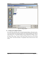
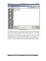
2.6
Loading Test Data
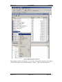
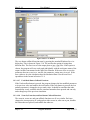
Test data can be loaded by pressing the open button on the toolbar that appears across
the top of the home window. The standard Windows Open dialog box will appear.
This is shown in Figure 2.9. In the Files of Type menu at the bottom of the window,
select Import Excel Test Data. Browse to the relevant file, select it, and press the open
button. The data will be plotted. The test data must be formatted in the manner
specified in 3.1.4.
May07-18
Basic Use
Page 7 of 73
May07-18
User Manual
4/24/2007
Figure 2.9 Loading Test Data
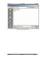
2.7
Saving and Loading Parameters
The values of the edit boxes can be saved and reimported during a subsequent session.
To save the parameters, click the save button on the toolbar that appears across the top
of the home screen. The standard Windows Save As dialog box will appear. This is
shown in Figure 2.10. Select Save Paramter Setting from the Files of Type menu at
the bottom of the window. Browse to the location where the files are to be saved and
enter a name. Press the Save button. The parameter values will be saved in a .mat
format.
May07-18
Basic Use
Page 8 of 73
May07-18
User Manual
4/24/2007
Figure 2.10 Saving Parameters
To open saved parameters from a previous session, press the Open button from the
toolbar. The standard Windows save as box will appear. This is shown in Figure
2.11. Select Load Parameter Setting from the Files of Type menu. Browse to the
folder containing the saved data, select the file, and press the Open button. The edit
box values and slider bar position will be changed accordingly.
May07-18
Basic Use
Page 9 of 73
May07-18
User Manual
4/24/2007
Figure 2.11 Opening Saved Parameter Settings
2.8
Saving Graphs and Exporting Simulation Data
The graphs and simulation data can also be exported. The graphs can be saved in jpeg
format. To do this press the save button on the toolbar. The standard Windows Save
As dialog box will appear. This is shown in Figure 2.12. Select Save Graphs from the
Save as Type menu. Browse to the location where the graphs are to be saved. Type a
file name and press the Save button. The graphs will be saved seperatly with the
variable’s workspace name appended to the filename that was entered.
May07-18
Basic Use
Page 10 of 73
May07-18
User Manual
4/24/2007
Figure 2.12 Saving Graphs
The simulation data can also be exported to an Excel file of the same format as the test
data. This can be done by pressing the Save button on the toolbar. The standard
Windows Save As dialog will appear. This is shown in Figure 2.13. Select “Save
Simulation Data as Spreadsheet” from the Save as Type Menu. Brows to the location
where the file is to be saved, enter a filename, and press the save button. The
simulation data will be saved as an Excel spreadsheet. If the simulation time is
particularly long, or the step size particularly small, the file size may be quite large.
Typically, 30 seconds of simulation data requires approximately 1 MB of disk space.
May07-18
Basic Use
Page 11 of 73
May07-18
User Manual
4/24/2007
Figure 2.13 Exporting Simulation Data
May07-18
Basic Use
Page 12 of 73
May07-18
User Manual
4/24/2007
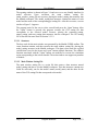
3 Program Structure
This section is intended to provide the reader with an in-depth background in the
program's structure and design. Complete source code appears on the accompanying
CD.
3.1
Design Overview
The software was developed in the Matlab programming language and was designed
for maximum flexibility. As a result of the modular design, the structure can be broken
into several independent components. An overview of each of these components
appears in Section 3.1 with a more detailed discussion of each in Sections 3.2 through
3.4.
The Matlab Graphical User Interface Development Environment (GUIDE) toolbox
was used to generate the base code for the three main GUI components. Code
generated using GUIDE contains a main function that executes the create function and
processes the user inputs. A callback function is provided for each object (button, drop
down menu, list box, edit box, slider bar, etc).
The layout function creates the GUI from standard Matlab components. A create
function is also provided for each object. The callback functions allow the programmer
to create code that will execute each time that a button is pressed, text is selected, or
information entered. The callback functions allow for the programmer to create code
that will execute when an object is created. The create functions were not used for this
project.
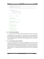
3.1.1 Program Components
The program can be broken down into three basic components, the graphical user
interface, the Simulink models, and the simulation scripts that connect them. The
Matlab workspace serves as a swap memory of sorts. In virtually every location where
one subprocess interfaces with another, variables are stored in the Matlab workspace
by one process and called by another. This greatly simplifies the calling of functions as
variables do not need to be explicitly passed. The simplified flow of information
between the basic program components is shown in Figure 3.1.
May07-18
Program Structure
Page 13 of 73
May07-18
User Manual
4/24/2007
Figure 3.1 Simplified Flow of Information
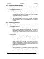
3.1.1.1 Basic Algorithm
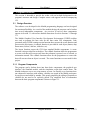
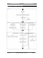
The basic algorithm is shown in Figure 3.2. After the initial program execution, the
opening window appears. The user selects a model and presses OK. The home screen
appears and the user imports test data and chooses to either batch simulate (run several
simulations at once with slight adjustments to one parameter) or to edit parameters
himself and simulate. The results are plotted with the test data and the user compares
the results. If they are satisfactory, he exits the program, if they are not, he can choose
to edit parameters or run more batch simulations. A more detailed version of this
flowchart appears in Appendix A.
May07-18
Program Structure
Page 14 of 73
May07-18
User Manual
4/24/2007
Figure 3.2 Simplified Flow Chart
3.1.1.2 Graphical User Interface
The graphical user interface is intended to provide the user with an easy means of
entering parameters and viewing selected simulation results. It also provides several
features such as the ability to undo or redo certain actions and import or export data
that make it much more user-friendly. It can be broken into three basic components;
the opening window (main_window.m), the home window (GUI.m), and the batch
simulation window (batch_simulation.m).
The basic purpose of the graphical user interface is to collect parameters from the user,
store them in the Matlab workspace, execute the simulation script, collect the arrays of
simulation data, and plot them.
3.1.1.3 Simulink Models
The Simulink models are block diagram representations of the state space equations
necessary for time domain simulations. It is very important that all constants be
entered in as variables to ensure that they can be easily changed and that they will be
changeable from the graphical user interface. Selected parameters are stored as arrays
in the Matlab workspace.
May07-18
Program Structure
Page 15 of 73
May07-18
User Manual
4/24/2007
The standard practice has been to use embedded Matlab functions for the algebraic
equations corresponding to the electrical network and loads. It is very important that
every integral have an initial condition defined. It is not necessary to use Simulink
models. Instead, a state space model could be formulated and one of the time domain
differential equation solvers could be used to solve the system.
3.1.1.4 Simulation Scripts
The simulation scripts are Matlab m-files that contain the equations necessary to
calculate the initial conditions. After all of the initial conditions have been calculated,
the Simulink model is executed.
3.1.2 The Matlab Workspace
The Matlab Workspace serves as a swap memory or information repository. Any
information that needs to be shared between subprocesses is sent to the base Matlab
workspace and then read in by the next process. This is intended to simplify function
calling.
3.1.3 Setting Files
Setting files are Matlab scripts that create data structures in the Matlab workspace.
They are intended to store default data needed to properly initialize the opening
window without requiring the user to enter it manually each time the program
executes. The main window setting file (main_window_setting_file.m) stores a list of
the models in the library and the names of their respective setting files.
The several GUI setting files are specific to each model. They contain the information
necessary to initialize the home screen including the name of each parameter in the
Matlab workspace, the name that is to be displayed on the window, the minimum
value of each slider bar, in addition to the maximum and default values. The GUI
setting files also contain the workspace and display names for each of the values that
are plotted and the names of each test, or simulation case, that the model can execute.
Each model must have its own setting file. While creating setting files can be tedious,
this method does allow the user to add models to the library without modifying the
base graphical user interface code or creating a newly coded graphical user interface.
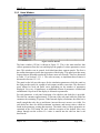
3.1.4 Test Data
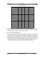
The program allows data to be plotted from Microsoft Excel spreadsheets. This data
must be saved in the .xls format and shall be arranged according to Table 3.1. It is
important that the first column correspond to time (in seconds) and the remaining
columns correspond to the outputs. There must be one and only one column for each
output. If no data is available, then that column should be left as zeros, but never
blank. The same format is used for exporting simulation data. A sample of test data
appears in Appendix B.
May07-18
Program Structure
Page 16 of 73
May07-18
User Manual
4/24/2007
Table 3.1 Sample Test Data Format
Time
0
1
2
3
Output #1 Output #2 Output #3 Output #4
0.1
0.2
0.4
0.8
0.2
0.4
0.6
1.6
0.3
0.6
0.8
2.4
0.4
0.8
1.2
3.2
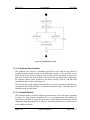
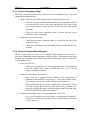
3.1.5 Interaction Between Components and Flow of Information
The flow of information between subprocesses is shown in detail in Figure 3.3.
Figure 3.3 Detailed Flow of Information
May07-18
Program Structure
Page 17 of 73
May07-18
User Manual
4/24/2007
As one can see, the Matlab workspace serves as the central information storage point.
All data that is shared among processes is entered into the Matlab workspace.
3.2
Graphical User Interface
The graphical user interface can be broken into three components; the opening
window (main_window.m), home window (GUI.m), and the batch simulation window
(batch_simulation.m). Each of these components is described in detail in Sections
3.2.2 through 3.2.4. A discussion on the data structures that store all of the information
necessary appears in Section 3.2.1. Complete source code appears on the
accompanying CD.
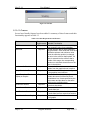
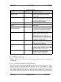
3.2.1 Data Structures
Several data structures are used throughout the program, a summary of these appears
in Table 3.2. The model_setting data structure is used by the opening window. There is
one data structure for the entire library. The parameter_setting data structure contains
the information needed for the parameters panel of the home screen. There is one
parameter_setting structure for each model. The output_setting structure contains the
information necessary for the output panel of the home screen. There is one
output_setting for each model. The tests_setting structure is again model specific and
contains the information necessary for the test selection menu on the home screen.
May07-18
Program Structure
Page 18 of 73
May07-18
User Manual
4/24/2007
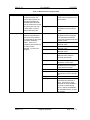
Table 3.2 Data Structures and their Fields
Structure
model_setting
parameter_setting
Purpose
Field
Stores the data needed by
model_name
the opening window; the
name of each model in the
library and the setting file
associated with that model.
There is one structure for the
setting_file_name
entire library and one entry
for each model. Found in
main window setting file.
Purpose
String value of the mode's name
as it should be displayed on the
home window.
workspace_name
String containing the name of
the parameter as it will appear
in the workspace and will be
used in the simulation script and
Simulink model.
Double containing the minimum
parameter value.
Double containing the maximum
parameter value.
Double containing the default
parameter value.
Double containing the previous
parameter value. Used for
undo/redo functionality.
Stores the data that is
needed for the parameters
panel on the home window.
This information is also used
by the batch simulation
window. There is one
structure for each model and
one entry for each
parameter. Found in GUI
setting file.
min_value
max_value
default_value
previous_value
current_value
display_name
description
color
slider_panel
editability
May07-18
Program Structure
String value of the setting file
associated with that particular
model.
Double containing the
parameters current value.
String containing the name of
the parameter as it will appear
on the parameters panel.
Not used on current versions.
A three double array that
determines the color of the edit
box.
Not used on current versions.
An integer that determines for
which tests the parameter is
active. If this is set to 0 the
parameter is always editable, if
it is set to a number greater
than 0, it will only be editable if
the test pulldown menu is set to
that position.
Page 19 of 73
May07-18
User Manual
4/24/2007
Table 3.2 Continued
Structure
output_setting
Purpose
Stores the data that is needed
for the ouput panel on the
home window. There is one
structure for each model and
one entry for each output.
Found in the GUI setting file.
Field
workspace_name
start_time
end_time
display_name
test_data
simulation_data
old_simulation_data
test_time
tests_setting
Stores the strings that are
test_name
needed for the test selection
menu on the parameter panel
of the home window. Found
in the GUI setting file.
Purpose
String containing the name of
the variable as it appears in the
Simulink block diagram and
workspace.
Not used on current versions.
Not used on current versions.
String containing the name that
is displayed on the graph's YDouble array containing the data
imported from the Excel
spreadsheets.
Double array containing the
simulation data.
Double array containing the data
from the previous simulation.
Double array containing the time
from the imported Excel data.
String containing the name of
the test as it is displayed in the
test selection pulldown menu.
3.2.2 Opening Window
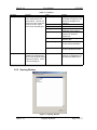
Figure 3.4 Opening Window
May07-18
Program Structure
Page 20 of 73
May07-18
User Manual
4/24/2007
The opening window is shown in Figure 3.4 and serves as a user friendly interface for
model selection. Upon execution, the main window setting file
(main_window_setting_file.m) executes, placing the model_setting data structure into
the Matlab workspace. The model_setting data structure contains the names of each
model and the name of the corresponding gui setting file. After this executes, a screen
similar to Figure 3.4 appears.
The program waits for the user to select a model and press the “Open” button. After
the “Open” button is pressed, the program executes the GUI setting file that
corresponds to the selected model executes, placing the parameter_setting,
output_setting, and tests_setting data structures into the workspace. The GUI setting
file is described in more detail in Section 3.2.3.2.
3.2.2.1 Structure
The base code for the main window was generated by the Matlab GUIDE toolbox. The
create function contains code that executes the main window setting file, placing the
model_setting structure in the Matlab workspace. This data is then read into a global
variable that is used in the layout and “open” button callback functions. The callback
function associated with the “Open” button was modified to execute the simulation
script corresponding to the selected model. The main window can support any number
of models.
3.2.2.2 Main Window Setting File
The main window setting file is a script file that creates a data structure named
model_setting and places it in the Matlab workspace. This data structure contains two
fields for each entry, one for the model’s name (model_name) and the other for the
name of the GUI setting file that corresponds to the model.
May07-18
Program Structure
Page 21 of 73
May07-18
User Manual
4/24/2007
3.2.3 Home Window
Figure 3.5 Home Window
The home window (GUI.m) is shown in Figure 3.5. This is the main interface that
collects parameters from the user and displays the graphs of various parameters versus
time. This window can, in general, be divided into three separate panels. The first is
the toolbar that appears across the top portion of the display. This panel provides many
features that are intended to make the software more user friendly. These are discussed
in Table 3.3 in Section 3.2.3.1.1. The code necessary to implement these features is
discussed in Section 3.2.3.1.2.
The panel on the left provides space for the simulation parameters while the panel on
the right provides space for a graph of each output variable versus time. The amount of
space allotted to each sub panel varies depending on the number of parameters
displayed. For every 16 parameters, an additional column of parameters is added and
an additional 6.8 percent of the display is allocated to parameters.
For each parameter, a sub panel consisting of an edit box and slider bar is provided.
The edit box consumes approximately 70 percent of the sub panel while the slider bar
consumes the remaining 30 percent. Under normal display resolutions, the slider bar is
small enough that only the up and down (increase/decrease) arrows are visible. For
each slider bar, there are default, minimum, maximum, and current values, which are
found in the parameter_setting data structure. The initial values of these properties are
contained in the GUI setting file and, with the exception of the default value, may
change through out the session. If a value is entered into the edit box that is not
between the
May07-18
Program Structure
Page 22 of 73
May07-18
User Manual
4/24/2007
Other important features in the parameters panel are the simulate and batch simulate
buttons and the drop down test selection menu. The simulate button places the
parameters in the workspace, executes the simulation script, collects and plots the
simulation results. The batch simulate button allows the user to run several
simulations at once, with one variable being changed each time. This allows the user
to visualize the effects of one parameter on the simulation results.
The test selection menu allows for several different events to be incorporated into one
model and display. (The models built thus far have three different tests; a step change
in reference voltage, a “load rejection” test in which the main breakers are opened, and
a three phase fault.) Each time that the simulate button is pressed, the entry selected in
the test menu is placed into the workspace as an integer, this is then collected by the
simulation script and a switch statement determines which initial conditions to use and
test to run. Because in real world testing situations, different tests may require
different initial conditions, the graphical user interface can make the edit box and
slider bar associated with certain parameters inactive based on the test selected in the
drop down menu. This is intended to reduce the possibility of entering a parameter in
the wrong edit box.
A sub panel is also provided for each output variable. Each sub panel has one plot box
that consumes approximately 85 percent of the horizontal space and 92 percent of the
vertical space. The sub panels are arranged in a stacked manner, with the horizontal (x)
axis being much longer than the vertical (y) axis in any case where more than one
graph is displayed.
3.2.3.1 Structure
A great deal of effort has been placed in making the entire graphical user interface as
flexible and easily expandable as possible. The home screen has been created in such a
way so as to in theory allow an infinite number parameters and plots, however, due to
space restrictions, the user should attempt to limit the number of parameters to 96 and
the plots to 6. The base code for the graphical user interface was created using GUIDE
by building a basic window with the toolbar, parameters panel, and graph panel and
then modifying the code to allow an infinite number of number of parameters and
graphs.
Upon execution, the parameter_setting, model_setting, and tests_setting data structures
are collected from the Matlab workspace and are saved as global variables. These are
used throughout the program. After the main window appears the interface waits for
user commands. After the simulate button is pressed, each parameter is placed in the
Matlab workspace as a double variable. An integer corresponding to the selected test is
placed in the workspace. The simulation script is executed, after this, the simulation
data is collected from the Matlab workspace and plotted. Because the exact number of
parameters or outputs is not fixed, loops were used. A wait bar (see Figure 3.6) is
provided to remind the user that the simulation is in process. To ensure that the wait
bar remains on top of all other Matlab windows, the window should be modal.
May07-18
Program Structure
Page 23 of 73
May07-18
User Manual
4/24/2007
Figure 3.6 Wait bar
3.2.3.1.1 Features
Several user friendly features have been added. A summary of these features and their
functionality appears in Table 3.3.
Table 3.3 Product Requirements and Features
Feature
Edit Box
Slider Bar
Interface with Simulink
Graph Simulation Data
Import Data from Excel and
Display on Graphs
Undo/Redo Actions
Save Current Session
Load Previous Session
Zoom In and Out on Graphs
May07-18
Required or
Supplemental Intended Functionality
Provide the user with a means to quickly
Required
enter a specific value for a parameter.
Provide the user with an easy method to
Required
vary parameters. Each slider bar shall have
a default maximum and minimum value.
When the slider bar position is changed,
the value in the edit box shall update. If a
value is entered into the edit box that is
outside of this range, the corresponding
maximum or minimum should reset to the
value in the edit box.
The user shall be able to execute Simulink
Required
models from the graphical user interface.
Simulation data shall be plotted on figures
Required
in the graphical user interface.
The user shall be able to import time
Required
domain data stored in Microsoft Excel
spreadsheets in a format specified by the
project team and plot them on the same
graphs as the simulation data.
The user shall be able to undo actions upto
Required
to previous simulation.
The user shall be able to save the position
Required
of each slider bar.
The user shall be able to load the position
Required
of each slider bar from a previous session.
The user shall be able to zoom in and out
Required
on all graphs.
Program Structure
Page 24 of 73
May07-18
User Manual
4/24/2007
Table 3.3 Continued.
Feature
Handle Simulation of
Different Tests
Handle Multiple Models
Pan Graphs
Save Graphs as Matlab
Figures
Export Simulation Data to
Excel Spreadsheet
Batch Simulation
Hold Previous Zoom Level
Graph Previous Simulation
Data
Color Code for Edit Box
Required or
Supplemental Intended Functionality
The graphical user interface shall be able to
Required
handle models capable of simulating
different events
The graphical user interface shall be
Required
capable of handling a library of any number
of models. The project team shall enter at
least 5 models into this library.
Supplemental The user should be able to pan graphs.
Supplemental The user should be able to save graphs as
Matlab figures.
Supplemental
The user should be able to save simulation
data as an Excel spreadsheet in a format
that is the same as the imported data.
Supplemental The user should be able to choose a single
parameter, specify a minimum and
maximum value, and any number of
simulations and have the program iterate
that many times between those two points
and graph the simulation data.
Supplemental When test data has been imported, the
Graph's zoom level should not change after
the simulate button is pressed.
Supplemental
The previous simulation data should appear
as a light gray line to allow the user to judge
progress in matching the test data.
Supplemental Color edit boxes to help user to visually
group different types of parameters
belonging to different subsystems.
3.2.3.1.2 Callback Functions
Callback functions are used to specify what actions should occur after a certain action
is performed.
3.2.3.1.2.1 Slider Bar and Edit Box Callback Functions
The slider bars share a common callback function. (The edit boxes do as well.) This is
possible because each slider bar and edit box has its own handle, a double
identification number that is unique to each object. The remaining buttons have their
own callback functions. The edit box callback function collects the new value from the
edit box and changes the position of the slider bar. The slider bar’s range is adjusted if
May07-18
Program Structure
Page 25 of 73
May07-18
User Manual
4/24/2007
necessary. The slider bar call back function contains code that updates the value in the
edit box and adjusts the position of the slider bar.
3.2.3.1.2.2 Test Selection Menu Callback Function
The test selection drop down menu call back function first deletes both the current and
old simulation data so that the gray trace associated with the previous simulation will
not appear when the simulation button is next pressed. Each parameter is then checked
to see if its status should be changed from active to inactive or vice versa.
3.2.3.1.2.3 Simulate Button Callback Function
The simulate button callback function first makes the simulate button inactive and
changes the text from “Simulate” to “Simulating…” Next a wait bar is created and
each parameter is placed in the workspace. If this test has been simulated previously,
the old simulation data is placed into the old_simulation_data field in the
output_setting data structure and the simulation is executed. If there is a problem with
the simulation, a catch statement will cause a message box displaying “Simulation
error” to appear. This is shown in Figure 3.7. This prevents the program from
crashing, but does not provide much insight into the source of the problem. If the
simulation executes properly, the results are plotted and a legend appears in the upper
right hand corner of the top plot box. A custom color scheme is defined to ensure that
all of the plots are legible and that all colors are pleasing to the eye.
Figure 3.7 Simulation Error Message Box
3.2.3.1.2.4 Batch Simulate Button Callback Function
May07-18
Program Structure
Page 26 of 73
May07-18
User Manual
4/24/2007
Figure 3.8 Batch Simulate Window
The batch simulate call back function starts by making the batch simulate button
inactive and changing the text from “Batch Simulate” to “Simulating…” The batch
simulation window appears and the program suspends execution until the user presses
either the OK or cancel button. The batch simulation window appears in Figure 3.8.
After this, the program resumes execution, if the cancel button was pressed, the
program returns to the main function and does not simulate. If the OK button was
pressed, a wait bar is displayed and the function collects the parameter, minimum
value, maximum value, and number of simulations from the workspace. After this an
array of parameter values for the parameter that will be varied is created and all of the
parameters are placed in the workspace. After the simulation has completed, the data
is plotted. The program repeats this for the desired number of simulations.
3.2.3.1.2.5 Open Button Callback Function
The open button callback function starts by opening the standard windows “Open
File” window. This window is shown in Figure 3.9. The user has the option to either
import test data from an Excel spreadsheet or load a saved case in the form of a
Matlab .mat file.
May07-18
Program Structure
Page 27 of 73
May07-18
User Manual
4/24/2007
Figure 3.9 Open Window
After the user has selected a file, the program attempts to open it as an Excel file, if it
succeeds, the data is plotted, if it fails, the program attempts to open it as a .mat save
case. If this succeeds, each parameter is set to the value in the file, if this fails as well,
an error message is displayed.
3.2.3.1.2.6 Save Button Callback Function
May07-18
Program Structure
Page 28 of 73
May07-18
User Manual
4/24/2007
Figure 3.10 Save As Window
The save button callback function starts by opening the standard Windows Save As
dialog box. This is shown in Figure 3.10. The user has the option of saving three
different files. The first is to save the output plots as jpeg (.jpg) files. If this option is
chosen, the program will save each graph individually with the workspace name of the
output variable concatenated to the end of the filename. If the user elects to save the
parameter data (save case) as a .mat file, the parameter_setting array is saved. If the
user wishes to save the simulation data, the simulation data is saved to an Excel
spreadsheet in the format in Section 3.1.4.
3.2.3.1.2.7 Undo/Redo Button Callback Functions
If the Undo toolbar button is pressed, the program changes the last modified parameter
to its previous value and enables the redo button. If the redo button is pressed, the last
undone parameter is changed to its pre-undo value. It should be noted that the undo
functionality is only available after the simulate button has been pressed and can only
undo changes up to the previous simulation.
3.2.3.1.2.8 Zoom In, Zoom Out, and Pan Button Callback Functions
The zoom in, zoom out, and pan callback functions are all very similar. Each one
changes the zoom property of each graph to either zoom in, zoom out or pan, disables
the button that was pressed, and enables the other two.
May07-18
Program Structure
Page 29 of 73
May07-18
User Manual
4/24/2007
3.2.3.2 GUI Setting File
The GUI setting file is a Matlab script that creates three data structures. The first,
parameter_setting, contains the data necessary for the slider bars and edit boxes. There
is one entry in this data structure for each slider bar or edit box on the parameters
panel. The next, output_setting, contains all of the information necessary for the
graphs on the output panel. The last, test_setting, contains the information needed for
the test selection menu. These data structures are described in detail in Table 3.2.
Three additional string variables, simulin_file_name, simulation_file, and
simulation_script, are also placed in the workspace. simulin_file_name contains the
name of the Simulink block diagram. simulation_file contains the title given to the
home window. simulation_script contains the name of the simuation script associated
with that particular model. An example setting file is included in Appendix C.
3.2.4 Batch Simulation Window
The batch simulation window, shown in Figure 3.8 allows users to run several
simulations at one time, varying one parameter each time. This is intended to allow the
user to see the effects of different values of one parameter and to aid in the overall
parameter selection process.
When the batch simulate button is pressed, the batch simulate window appears. A pull
down menu allows the user to select which parameter will be varied. The maximum
and minimum values correspond to the points between which the program will iterate.
By default, these are set at the minimum and maximum slider bar values. A callback
function ensures that when the position of the pull down menu changes, that the
maximum and minimum values will change. The simulations edit box allows the user
to set the number of times that the program will run. This number must be an integer
greater than 1.
When the OK button is pressed five variables are passed to the Matlab workspace.
parameter, is an integer corresponding to the parameter selected in the pull down
menu. The maximum value, max, the minimum value, min, the number of simulations,
simulations, and an exit flag cancel. If cancel is set to 1, because the cancel button
was pressed, the home screen will not run the simulation, if the OK button is pressed,
cancel will be set to 0 and the home screen will run the simulations.
3.3
Simulation Scripts
The simulation scripts are Matlab scripts that collect parameters from the workspace,
determine which test to run, and initial conditions to use, calculates additional initial
conditions, and executes the Simulink model.
Though these scripts are very flexible, the standard practice has been to use a switch
statement that switches based on the test selected. The initial conditions corresponding
to this test are chosen in this statement. In the lines that follow, more initial conditions
are calculated using algebraic expressions. The last line executes the Simulink model.
It is very important that the variables used in the simulation script exactly match the
May07-18
Program Structure
Page 30 of 73
May07-18
User Manual
4/24/2007
variables used in the Simulink models and GUI setting files. An example has been
included in Appendix E.
It should be noted that it is not necessary to use Simulink block diagrams. The
simulation script can be used to build a state space model of the system being studied.
Any one of the Matlab differential equation solvers can be used to perform the
simulation.
3.4
Simulink Model
The Simulink models used for simulations are also very flexible. They can be models
of any dynamic system and do not need to be from the power industry. The standard
practice has been to use block diagrams for the generator windings, exciters, voltage
regulators, turbines, and governors and imbedded Matlab code for the algebraic
equations corresponding to the electrical network.
The simulation time and step size need to be adjustable via the home screen, thus the
appropriate settings in the configuration parameters dialog box (Simulation ->
Configuration Parameters) need to be changed to variables. Variables will be used in
place of constants on all blocks in the algebraic equations in order to maximize
flexibility. A sample Simulink block diagram appears in Appendix D.
May07-18
Program Structure
Page 31 of 73
May07-18
User Manual
4/24/2007
4 Program Maintenance
This section is intended to serve as a guide and reference manual for product
maintenance. It includes information examples on how to add models to the library
and modify existing models.
4.1
Adding Models to Library
This section will discuss the process used to add models to the library. The process
basically consists of creating the Simulink model and simulation script, creating the
GUI setting file, and editing the Main Window setting file. These are described in
more detail Sections 4.1.1 through 4.1.4. An example appears in Section 4.1.5.
Before reading this section, the reader should study Table 3.2, a description of all of
the data structures used in the program.
4.1.1 Compatible Simulink Models
A compatible Simulink model has several characteristics, the first is that all parameters
must be entered in as variables. The name that it is used in the Simulink model will be
referred to as the workspace name. This name should be the same name that is used in
the “workspace_name” field of the parameter_setting data structure. The model must
also have the simulation stop time set to Tstop and the fixed step size must be set to
Step_Size. The solver type should be set to fixed-step. Standard practice has been to
use the ODE-3 solver. The can be set in the Configuration Parameters dialog box.
This can be found in the Simulink Simulation menu.
All data that the user wishes to plot should be connected to a “To Workspace” block.
The variable name should be set to the same that appears in the “workspace_name”
field of the “output_setting” data structure. The save format field should be set to
array.
Initial conditions can be imported from the workspace using “constant” blocks. The
“constant value” field should be set to the name as it appears in the simulation script.
It is very important that every integral have an initial condition. A sample block
diagram appears in Appendix C.
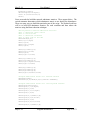
4.1.2 Compatible Simulation Scripts
Simulation scripts are files that calculate initial conditions and determine which test to
simulate. These files are very flexible though the generally excepted form is to have
the first few lines be a switch statement that determines which test to execute.
The variable to be switched is test_switch. This variable is an integer that is
determined based on the position of the test pull down menu when the simulate button
is pressed. The order that the tests appear in, and thus the value of test_switch that
corresponds to a particular test is determined by its index in the test_setting menu.
The generally excepted order is voltage step, load rejection and three phase fault. The
generally excepted switch statement appears below and is applicable to all generator
models.
May07-18
Program Maintenance
Page 32 of 73
May07-18
User Manual
4/24/2007
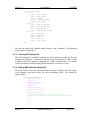
switch test_switch
case 1
pgen = Pgen_Vstep;
qgen = Qgen_Vstep;
vm = V1_Vstep;
vstep = .01*Vup_Vstep;
tstep = Tup_Vstep;
case 2
pgen = Pgen_Ld_Reject;
qgen = Qgen_Ld_Reject;
vm = V1_Ld_Reject;
ton = Treject_Ld_Reject;
case 3
pgen = Pgen_Flt;
qgen = Qgen_Flt;
vm = V1_Flt;
ton = T_flt_on;
toff = T_flt_off;
end
The last line executes the Simulink model using the “sim” command. The simulation
scripts appear in Appendix I.
4.1.3 Creating GUI Setting File
The GUI setting file is a Matlab script that sets up the databases needed for the main
graphical user interface. A summary of these data structures appears in Table 3.2 and
a sample setting file appears in Appendix B. When adding models, it is usually
quicker and easier to edit an existing setting file than it is to start a new one.
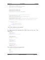
4.1.4 Editing Main Window Setting File
The main window setting file contains the data necessary to display all of the models
in the opening screen and execute the correct simulation script. The current file
appears below.
model_setting=struct(...
'model_name',{...
'Genrou',...
'Genrou exst4b',...
'Genrou rexs',...
'Gensal',...
'Gensal exst1',...
'Gensal exst1 Hygov'
},...
'model_folder',{...
%folder containing all the necessary files
%it should be located inside the current directory
''...
''...
''...
''...
''...
May07-18
Program Maintenance
Page 33 of 73
May07-18
User Manual
4/24/2007
''
},...
'setting_file_name',{...
'genrou_setting_file',...
'genrou_exst4b_setting_file',...
'genrou_rexs_setting_file',...
'gensal_setting_file',...
'gensal_exst1_setting_file',...
'gensal_exst1_hygov_setting_file',
}...
);
The ‘model_name’ field is the name of the model as it appears in the model list on the
opening window. If a model is added the model’s name should be added in quotation
marks at the end of the list. The ‘model_folder’ field is no longer used, if a model is
added, empty quotation marks should be added at the end of the list. The
“setting_file_name” should be the name of the GUI setting file that corresponds to
this model the should be added in quotation marks at the end of the list with out the
“.m.”
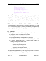
4.1.5 Example: Creation and Addition of Classical Machine vs. Infinite Bus
In order to illustrate the concepts laid out in Sections 4.1.1 through 4.1.4, the reader
will be walked through an example of creating a Simulink model and simulation script
that are compatible with the GUI and then adding them to the library. The example
will be the classical machine against an infinite bus.
4.1.5.1 Preparation
The following data must be collected before beginning to create the model:
•
A basic block diagram of the model must be prepared.
•
Detailed equations to calculate initial conditions.
•
Equations linking the block diagram to the rest of the network.
•
A list of all tests that need to be built into the model and displayed on the GUI.
•
A list of all parameters that need to be displayed on the graphical user
interface. This information should include:
o The name of each parameter.
o A default value for each parameter.
o A minimum value for each parameter.
o A maximum value for each parameter.
•
A list of all simulation results that need to be plotted.
The following data has been prepared for the classical machine against an infinite bus.
A block diagram of the classical model appears in Figure 4.1.
May07-18
Program Maintenance
Page 34 of 73
May07-18
User Manual
4/24/2007
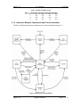
Figure 4.1 Block Diagram of Classical Model
It will be assumed that the user will supply the starting terminal voltage and real and
reactive power generation. It will be assumed that the voltage angle at the machine
terminals will be zero, the initial power angle and voltage angle at the infinite bus will
be adjusted accordingly. The following equations can be used to calculate the initial
conditions:
S = P1+j*Q1
I = conj(S/V1);
E=abs(V1+zgen*I);
deltao=angle(V1+zgen*I);
Vinf= V1-(ztran+zline)*I;
The model needs to simulate load rejections and three phase fault, standard practice is
to simulate a voltage step as well. This is not logical for the classical model. The
equations to do this appear in Section 4.1.5.3. The basic technique is to develop
admittance matrices for the three scenarios (pre-fault, faulted, load rejected) networks
and reduce them using the Kron reduction technique.
The following equations can be used to connect the block diagram to the infinite bus:
I=Ybus*[E(cos(delta)+j*sin(delta));Vinf];
Pe=real(E1*conj(I(1,1)));
Te=Pe*w;
V1=EI(1,1)*(ra+j*xpd);
A lot of data besides the generator parameters need to be displayed on the GUI. These
include the simulation stop time and step size, the initial conditions for each test, the
system power and frequency bases, the disturbance time for each test, and the
impedances of network components such as the transmission line and transformer.
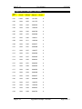
The data needed to create the GUI setting file appears in Table 4.1.
May07-18
Program Maintenance
Page 35 of 73
May07-18
User Manual
4/24/2007
Table 4.1 GUI Parameters
Workspace Name
h
d
ra
xpd
pgen_fault
qgen_fault
v1_fault
t_fault_on
t_fault_off
zfault
pgen_reject
qgen_reject
v1_reject
t_reject
mva_base
fbase
rl
xl
rt
xt
Tstop
Step_size
Minimum
1
0
0
0.1
0
-500
0
0
0
0
0
-500
0
0
1
50
0
0.001
0
0.001
1
0.0001
Default Maximum Display Name
3
7H
1
2D
0.05
0.05 Ra
0.2
0.5 Xpd
100
500 P_fault
30
500 Q_fault
1
1.05 V1_fault
1
10 t_flt_on
1.1
10 t_flt_off
0
10 Zfault
100
500 P_rjct
30
500 Q_rjct
1
1.05 V1_rjct
1
10 t_reject
100
500 S_Base
60
60 fbase
0.2
0.5 Rl
0.2
1 Xl
0.1
0.5 Rt
0.5
1 Xt
30
60 Tstop
0.005
0.01 Step_size
Standard practice is to plot the terminal voltage, field voltage, field current, and speed.
Because the classical model does not have field voltage or current, we will plot
terminal voltage, rotor angle, speed, and real power output.
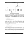
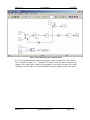
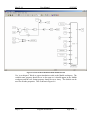
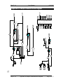
4.1.5.2 Creation of Simulink Model
This section will outline the creation of the Simulink block diagram. The first step in
creating the model is to enter the basic block diagram into Simulink. This is shown in
Figure 4.2. Using to and from blocks can clean up the block diagram and make it
more apparent, what is happening. The bottom set of blocks create a complex number
that will be used later to determine the current that is supplied. It can be difficult to
create complex numbers in imbedded Matlab functions, the standard practice is to
combine the magnitude and angle outside of the imbedded Matlab function.
May07-18
Program Maintenance
Page 36 of 73
May07-18
User Manual
4/24/2007
Figure 4.2 Basic Block Diagram as Simulink Model
It is very important that the right most integral’s initial condition be set to “deltao.”
This is shown in Figure 4.3. Normally all integrals need an initial condition, the
output of the right initial condition corresponds to the speed deviation, this initial
condition is zero because it is assumed that the machine is starting from its base speed.
May07-18
Program Maintenance
Page 37 of 73
May07-18
User Manual
4/24/2007
Figure 4.3 Integral Initial Condition
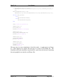
The next step is to add an imbedded Matlab function that connects the generator to the
network. This function will use some of the equations gathered in Section 4.1.5.1.
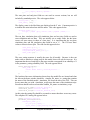
The complete text of the embedded Matlab function appears below.
function [Te,V1,Pgen] =
network(E,w,Vinf,Time,Ton,Toff,Ypre,Ydist,zgen,fbase)
%Calculate currents
if (Time<Ton)||(Time>=Toff)
I=Ypre*[E;Vinf];
else
I=Ydist*[E;Vinf];
end
%Find voltage at generator terminals
Vt=E-zgen*I(1,1);
%Find the real power injection from the generator
Pgen=real(Vt*conj(I(1,1)));
May07-18
Program Maintenance
Page 38 of 73
May07-18
User Manual
4/24/2007
%perunitize speed
wpu=w/(2*pi*fbase);
%Find the electrical torque supplied by the generator
Te=Pgen/wpu;
V1=abs(Vt);
A screen shot of the imbedded Matlab function appears in Figure 4.4.
Figure 4.4 Imbedded Matlab Function
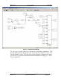
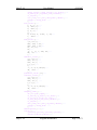
This should be connected to the rest of the block diagram as shown in Figure 4.5.
“From” blocks should be used for Ecomplex and w. For the constants, use a
“constant” block and change the value to the variable name as it will appear in the
Matlab workspace. The “clock” block should be used to import the time into the
embedded Matlab function. A “to” block should be used to connect the electrical
torque with the rest of the network.
May07-18
Program Maintenance
Page 39 of 73
May07-18
User Manual
4/24/2007
Figure 4.5 Classical Model With Embedded Matlab Function
Use “to workspace” blocks to export simulation results to the Matlab workspace. The
variable name property should be set to the name as it should appear in the Matlab
workspace and the save format property should be set to Array. The defaults can be
used for all other properties. This is shown in Figure 4.6.
May07-18
Program Maintenance
Page 40 of 73
May07-18
User Manual
4/24/2007
Figure 4.6 To Workspace Settings
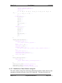
In this model we will need to place five variables in the Matlab workspace, the
machine angle, delta, the machine speed, speed, the real power generation, pgen, and
the terminal voltage, V1, are the variables that will be plotted, it is also very important
that the simulation time be exported to the workspace as well. This is shown in Figure
4.7.
May07-18
Program Maintenance
Page 41 of 73
May07-18
User Manual
4/24/2007
Figure 4.7 Completed Classical Model
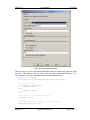
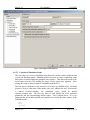
The last step in model creation is to modify the configuration parameters. The
Configuration Parameters dialog box can be found under the “Simulation” menu. The
stop time should be set to Tstop, the solver options should be changed to fixed-step,
the ode3 solver is typically used, the fixed-step size should be set to Step_size. This is
shown in Figure 4.8.
May07-18
Program Maintenance
Page 42 of 73
May07-18
User Manual
4/24/2007
Figure 4.8 Configuration Parameters
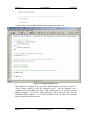
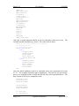
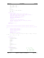
4.1.5.3 Creation of Simulation Script
The next step is to create a simulation script that will calculate initial conditions and
execute the Simulink model. Standard practice has been to create a simulation script
that can be executed without the graphical user interface. This allows the model to be
tested apart from the GUI, making the source of any errors more apparent. After
testing, the script is edited to make it compatible with the GUI.
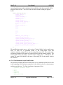
The first step in simulation script creation is to create a new Matlab m-file. Standard
practice is to give it the name of the model with “sim” added to the end. If the model
is named classical_machine, the simulation script would be named
classical_machine_sim. The first few lines of code should list of all generator
parameters and the corresponding default values. This is shown below. It is very
important that all variables spelled and capitalized in exactly the same manner as the
Simulink model.
h=3;
d=1;
ra=0.05;
May07-18
Program Maintenance
Page 43 of 73
May07-18
User Manual
4/24/2007
xpd=0.2;
pgen_fault=100;
qgen_fault=30;
v1_fault=1;
t_fault_on=1;
t_fault_off=1.1;
zfault=0;
pgen_reject=100;
qgen_reject=30;
v1_reject=1;
t_reject=2;
mva_base=100;
fbase=60;
rl=0.2;
xl=0.2;
rt=0.1;
xt=0.5;
Tstop=30;
Step_size=0.005;
After this a switch statement should be used to determine which test to run. The
switched variable should be test_switch. The code for this is below.
%Flag to set which test will be executed
%1= Load Rejection
%2= Three Phase Fault
switch test_switch
case 1
P1=pgen_fault;
Q1=qgen_fault;
V1=v1_fault;
Ton=t_fault_on;
Toff=t_fault_off;
case 2
P1=pgen_reject;
Q1=qgen_reject;
V1=v1_reject;
Ton=t_reject;
Toff=100000;
end
Next, the initial conditions need to be calculated, these were determined in Section
4.1.5.1. The complete equations can be found below. The data for real and reactive
power were supplied in terms of MW and MVAR, they will be perunitized here. The
base frequency will also be computed in rad/s.
ztran=rt+1j*xt;
zline=rl+1j*xl;
Zgen=ra+1j*xpd;
wo=2*pi*fbase;
P1=P1/mva_base;
Q1=Q1/mva_base;
S = P1+1j*Q1;
I = conj(S/V1);
May07-18
Program Maintenance
Page 44 of 73
May07-18
User Manual
4/24/2007
E=abs(V1+I*Zgen);
deltao=angle(V1+I*Zgen);
Vinf= V1-(ztran+zline)*I;
Tm=P1;
Lines are needed to build the network admittance matrices. These appear below. The
switch statement determines which admittance matrix to use during the disturbance.
There are many ways to build this particular part of the script. The method used here
will be to build full admittance matrices for each condition and then reduce the
matrices using the Kron reduction technique.
%Build prefault network admittance matrices
%Bus 1- Generator ideal source
%Bus 2- Infinite bus
%Bus 3- Generator Terminals
%Bus 4- High side of the GSU
Ybus=zeros(4,4);
Ybus(1,1)=1/Zgen;
Ybus(1,2)=0;
Ybus(1,3)=-1/Zgen;
Ybus(1,4)=0;
Ybus(2,1)=Ybus(1,2);
Ybus(2,2)=1/zline;
Ybus(2,3)=0;
Ybus(2,4)=-1/zline;
Ybus(3,1)=Ybus(1,3);
Ybus(3,2)=Ybus(2,3);
Ybus(3,3)=1/Zgen+1/ztran;
Ybus(3,4)=-1/ztran;
Ybus(4,1)=Ybus(1,4);
Ybus(4,2)=Ybus(2,4);
Ybus(4,3)=Ybus(3,4);
Ybus(4,4)=1/ztran+1/zline;
%Prepare Admittance matrix for faulted network
Ybusfault=Ybus;
Ybusfault(4,4)=Ybus(4,4)+1/(zfault+.0000001);
%Prepare admittance matrix for load rejected network
Ybusreject=zeros(4,4);
Ybusreject(1,1)=1/Zgen;
Ybusreject(1,2)=0;
Ybusreject(1,3)=-1/Zgen;
Ybusreject(1,4)=0;
Ybusreject(2,1)=Ybus(1,2);
Ybusreject(2,2)=1/zline;
Ybusreject(2,3)=0;
Ybusreject(2,4)=-1/zline;
Ybusreject(3,1)=Ybus(1,3);
May07-18
Program Maintenance
Page 45 of 73
May07-18
User Manual
4/24/2007
Ybusreject(3,2)=Ybus(2,3);
Ybusreject(3,3)=1/Zgen+1/(99999999);
Ybusreject(3,4)=-1/(99999999);
Ybusreject(4,1)=Ybus(1,4);
Ybusreject(4,2)=Ybus(2,4);
Ybusreject(4,3)=Ybus(3,4);
Ybusreject(4,4)=1/ztran+1/(99999999);
%Use Kron reduction to reduce admittance matrix
Yprereduced=Ybus(1:2,1:2)Ybus(1:2,3:4)*inv(Ybus(3:4,3:4))*Ybus(3:4,1:2);
Yreject=Ybusreject(1:2,1:2)Ybusreject(1:2,3:4)*inv(Ybusreject(3:4,3:4))*Ybusreject(3:4,1:2);
Yfault=Ybusfault(1:2,1:2)Ybusfault(1:2,3:4)*inv(Ybusfault(3:4,3:4))*Ybusfault(3:4,1:2);
switch test_switch
case 1
Ydisturbance=Yfault;
case 2
Ydisturbance=Yreject;
end
Next, a line is needed to run the simulation.
sim('classical_machine')
For testing purposes, plot commands will be added to the end of the code. These
appear below.
subplot(4,1,1)
plot(Time,V1)
ylabel('Terminal Voltage')
subplot(4,1,2)
plot(Time,delta)
ylabel('Rotor Angle')
subplot(4,1,3)
plot(Time,w)
ylabel('Speed')
subplot(4,1,4)
plot(Time,pgen)
xlabel('Time (s)')
ylabel('Pgen')
The completed simulation script appears below.
%Default parameter values
h=3;
d=1;
ra=0.05;
xpd=0.2;
May07-18
Program Maintenance
Page 46 of 73
May07-18
User Manual
4/24/2007
pgen_fault=100;
qgen_fault=30;
v1_fault=1;
t_fault_on=1;
t_fault_off=1.1;
zfault=0;
pgen_reject=100;
qgen_reject=30;
v1_reject=1;
t_reject=2;
mva_base=100;
fbase=60;
rl=0.2;
xl=0.2;
rt=0.1;
xt=0.5;
Tstop=30;
Step_size=0.005;
%Flag to set which test will be executed
%1= Three Phase Fault
%2= Load Rejection
test_switch=2;
switch test_switch
case 1
P1=pgen_fault;
Q1=qgen_fault;
V1=v1_fault;
Ton=t_fault_on;
Toff=t_fault_off;
case 2
P1=pgen_reject;
Q1=qgen_reject;
V1=v1_reject;
Ton=t_reject;
Toff=100000;
end
ztran=rt+1j*xt;
zline=rl+1j*xl;
Zgen=ra+1j*xpd;
wo=2*pi*fbase;
P1=P1/mva_base;
Q1=Q1/mva_base;
S = P1+1j*Q1;
I = conj(S/V1);
E=abs(V1+I*Zgen);
deltao=angle(V1+I*Zgen);
Vinf= V1-(ztran+zline)*I;
Tm=P1;
%Build prefault network admittance matrices
%Bus 1- Generator ideal source
May07-18
Program Maintenance
Page 47 of 73
May07-18
User Manual
4/24/2007
%Bus 2- Infinite bus
%Bus 3- Generator Terminals
%Bus 4- High side of the GSU
Ybus=zeros(4,4);
Ybus(1,1)=1/Zgen;
Ybus(1,2)=0;
Ybus(1,3)=-1/Zgen;
Ybus(1,4)=0;
Ybus(2,1)=Ybus(1,2);
Ybus(2,2)=1/zline;
Ybus(2,3)=0;
Ybus(2,4)=-1/zline;
Ybus(3,1)=Ybus(1,3);
Ybus(3,2)=Ybus(2,3);
Ybus(3,3)=1/Zgen+1/ztran;
Ybus(3,4)=-1/ztran;
Ybus(4,1)=Ybus(1,4);
Ybus(4,2)=Ybus(2,4);
Ybus(4,3)=Ybus(3,4);
Ybus(4,4)=1/ztran+1/zline;
%Prepare Admittance matrix for faulted network
Ybusfault=Ybus;
Ybusfault(4,4)=Ybus(4,4)+1/(zfault+.0000001);
%Prepare admittance matrix for load rejected network
Ybusreject=zeros(4,4);
Ybusreject(1,1)=1/Zgen;
Ybusreject(1,2)=0;
Ybusreject(1,3)=-1/Zgen;
Ybusreject(1,4)=0;
Ybusreject(2,1)=Ybus(1,2);
Ybusreject(2,2)=1/zline;
Ybusreject(2,3)=0;
Ybusreject(2,4)=-1/zline;
Ybusreject(3,1)=Ybus(1,3);
Ybusreject(3,2)=Ybus(2,3);
Ybusreject(3,3)=1/Zgen+1/(99999999);
Ybusreject(3,4)=-1/(99999999);
Ybusreject(4,1)=Ybus(1,4);
Ybusreject(4,2)=Ybus(2,4);
Ybusreject(4,3)=Ybus(3,4);
Ybusreject(4,4)=1/ztran+1/(99999999);
%Use Kron reduction to reduce admittance matrix
Yprereduced=Ybus(1:2,1:2)Ybus(1:2,3:4)*inv(Ybus(3:4,3:4))*Ybus(3:4,1:2);
May07-18
Program Maintenance
Page 48 of 73
May07-18
User Manual
4/24/2007
Yreject=Ybusreject(1:2,1:2)Ybusreject(1:2,3:4)*inv(Ybusreject(3:4,3:4))*Ybusreject(3:4,1:
2);
Yfault=Ybusfault(1:2,1:2)Ybusfault(1:2,3:4)*inv(Ybusfault(3:4,3:4))*Ybusfault(3:4,1:2);
switch test_switch
case 1
Ydisturbance=Yfault;
case 2
Ydisturbance=Yreject;
end
sim('classical_machine')
subplot(4,1,1)
plot(Time,V1)
ylabel('Terminal Voltage')
subplot(4,1,2)
plot(Time,rad2deg(delta))
ylabel('Rotor Angle')
subplot(4,1,3)
plot(Time,speed)
ylabel('Speed')
subplot(4,1,4)
plot(Time,Pgen)
xlabel('Time (s)')
ylabel('Pgen')
The next step is to run a simulation to check the results. A graph appears in Figure
4.9. These appear to be logical, the next step is to create a GUI setting file. The
Simulink model and simulation script should be copied into the directory containing
the main graphical user interface and library files.
May07-18
Program Maintenance
Page 49 of 73
May07-18
User Manual
4/24/2007
Terminal Voltage
1.2
1.1
1
0.9
0.8
0
5
10
15
20
25
30
0
5
10
15
20
25
30
0
5
10
15
20
25
30
0
5
10
15
Time (s)
20
25
30
Rotor Angle
100
50
0
-50
377.02
377
376.99
376.98
376.97
1.5
1
Pgen
Speed
377.01
0.5
0
Figure 4.9 Simulation Results
4.1.5.4 Creation of GUI Setting File
The GUI setting file is a Matlab script that sets up the data structures needed by the
GUI to properly initialize. The fields needed are described in Table 3.2. If the model
to be added utilizes either the Genrou or Gensal models, the setting file for these
models can be copied and modified as needed. This can save a great deal of time. In
this case, the model to be added is not similar to an existing setting file, a new one will
be created from scratch.
The first step is to create a new m-file. This should be saved in the same folder as the
main graphical user interface and library files as “classical_machine_setting_file.m.”
The first few lines of code should clear and set up a structure called parameter_setting.
These lines appear below:
clear parameter_setting;
parameter_setting=struct(...
This structure will have 11 fields, workspace_name, min_value, max_value,
default_value, previous_value, current_value, display_name, description, color,
May07-18
Program Maintenance
Page 50 of 73
May07-18
User Manual
4/24/2007
slider_panel, and editability. The next step is to create the workspace_name field.
This field should contain the name of each variable as it is used in the simulation
script and block diagram. The order that these appear in is of great strategic
importance as it is the order in which they will appear on the main GUI and should be
maintained for future fields. The standard practice has been to group the parameters
into several broad groups including generator parameters, initial conditions (terminal
voltage and real and reactive power injections for each test), test or disturbance
parameters (fault impedance, disturbance time, etc), network parameters (network
impedances and base power and frequency), simulation parameters, and parameters
corresponding to any applicable subsystems such as an exciter or a turbine/governor
model. The code for the workspace_name field appears below.
'workspace_name',{...
'h','d','ra','xpd',...
'pgen_fault','qgen_fault','v1_fault',...
'pgen_reject','qgen_reject','v1_reject',...
't_fault_on','t_fault_off','zfault',...
't_reject',...
'rt','xt','rl','xl','mva_base','fbase',...
'Tstop', 'Step_size' ...
},...
The next step is to create the min_value field. This field contains the minimum values
for each slider bar on the main GUI. It is very important that the entries in this field
be in the same order as the workspace_name field. The minimum values were
previously determined and appear in Table 4.1. The code appears below.
'min_value',{...
1, 0, 0, .1,...
0, -500, 0,...
0, -500, 0,...
0, 0, 0,...
0,...
0, 0.001, 0, 0.001, 1, 50,...
1, .0001 ...
},...
The next field is the max_value field. This field contains the maximum value of each
slider bar. These values were previously determined and appear in Table 4.1. The
code appears below.
'max_value',{...
7,2,.05,.5,...
500, 500, 1.05,...
500, 500, 1.05,...
10, 10, 10,...
10,...
.5, 1, .5, 1, 500, 60,...
60, .01,...
},...
The next field contains the information needed to set the default values for each edit
box.
'default_value',{...
May07-18
Program Maintenance
Page 51 of 73
May07-18
User Manual
4/24/2007
3,1,.05,.2,...
100, 30, 1,...
100, 30, 1, ...
1,1.1,0, ...
1,...
.1,.5,.2,.2,100,60,...
30, .005 ...
},...
The previous_value field contains information for the undo/redo commands. In the
setting file it is set to 0. The code for this appears below.
'previous_value',{0},...
In the setting file, current_value field is the same as the default_value field. These
may be changed in The code for this appears below.
'current_value',{...
3,1,.05,.2,...
100, 30, 1,...
100, 30, 1, ...
1,1.1,0, ...
1,...
.1,.5,.2,.2,100,60,...
30, .005 ...
},...
The next field, display_name is the name of each parameter as it will appear on the
GUI. These do not need to be the same as the workspace name or the variables in the
Simulink model or Simulation script, but a knowledgeable user should be able to
understand what it is without trouble. Be sure that the name is not more than 7 or 8
characters long as this can make the parameter titles appear to run together. The code
for the display names appears below.
'display_name',{...
'H','D','Ra','Xpd',...
'P_fault','Q_fault','V1_fault',...
'P_rjct','Q_rjct','V1_rjct',...
't_flt_on','t_flt_off','Zfault',...
't_reject',...
'Rt','Xt','Rl','Xl','S_base','fbase',...
'Tstop', 'Step_size' ...
},...
The description field is not currently used, but is still included as an empty field.
'description',{''},...
The color field determines the color of the edit box. This feature is intended to help
the user visually group certain parameters and find the parameter that he wishes to
adjust more quickly. This field can be any of the standard Matlab colors such as
‘yellow’ or ‘white’, or can be a 1 row, 3 column matrix that sets the colors that the
colors manually. The colors should be fairly light and transparent to allow the text in
the edit box to be readable. If the parameters are laid out well and pleasing colors are
chosen, this can be a very useful feature. The standard practice has been to use yellow
for generator parameters, white for initial conditions, red for network parameters,
May07-18
Program Maintenance
Page 52 of 73
May07-18
User Manual
4/24/2007
purple for simulation settings, green for exciter parameters and blue for
turbine/governor parameters. The code for this field appears below.
'color',{...
'yellow','yellow','yellow','yellow',...
'white','white','white',...
'white','white','white',...
'white','white','white'...
'white',...
[1 .4 .4],[1 .4 .4],[1 .4 .4],[1 .4 .4],[1 .4 .4],[1 .4 .4],...
[.7 .7 .9],[.7 .7 .9] ...
},...
The slider_panel field was once used to group the parameters into sub-panels though
this field is no longer used, standard practice has been to continue including it. The
code for this appears below.
'slider_panel',{...
1,1,1,1,...
2,2,2,...
2,2,2,...
2,2,2,...
2,...
3,3,3,3,3,3,...
4,4 ...
},...
The last field in the parameter_setting structure is the editability field. This field is
made up of integers. A 0 means that that particular parameter is editable regardless of
the position of the test menu. If the value is set to 1 it will be editable only when the
test menu is set to position 1, if the value is set to 2, it will only be editable when the
test menu is set to 3, etc. The code for this appears below.
'editability',{...
0,0,0,0,...
1,1,1,...
2,2,2,...
1,1,1,...
2,...
0,0,0,0,0,0,...
0,0 ...
}...
);
Next, the script should be executed to make sure that there is not a problem. The most
common errors in setting files result from one of the field having more entries than the
others. If this error occurs, count the number of entries in each field.
The output_setting field is normally the same for all models, unfortunately, the
standard outputs are not logical for this model. The output_setting structure contains
the information needed for the plots. The workspace_name field contains the names
of the arrays that will be plotted as they appear in the Simulink model. The code for
this appears below.
output_setting=struct(...
'workspace_name',{...
May07-18
Program Maintenance
Page 53 of 73
May07-18
User Manual
4/24/2007
'V1','Pgen','delta','speed'...
},...
The start_time and end_time fields are not used in current versions, but are still
included by standard practice. The code appears below.
'start_time', {0},...
'end_time', {10},...
The display_name is the label that gets displayed on the Y axis. Common practice is
to indicate the units in brackets after the name. This code appears below.
'display_name', {...
'V1 [pu]','Pgen [pu]','Delta [rad]','speed [rad/s]'...
},...
The test_data, simulation_data, old_simulation_data, and test_time fields are used to
store simulation and test data. They are initially set to empty fields, but the home
screen will store arrays in them at a later time. It is important that the test_data,
simulation_data, and old_simulation_data fields be set to ‘x’. The GUI uses these
values to choose what to plot. The code for this appears below.
'test_data',{'x'},...
'simulation_data',{'x'},...
'old_simulation_data',{'x'},...
'test_time',{0}...
);
The tests_setting structure is usually the same for all models. Because it does not
make sense to simulate a voltage step for this model, there will only be two tests. It is
important that the test listed first be the same test that corresponds to an editablity of 1
in the parameter_setting.editability field. The code appears below.
tests_setting=struct(...
'test_name',{...
'Three Phase Fault','Load Rejection'...
}...
);
The last three lines store information about where the model files are located and what
the title on the home window should be. simulin_file_name is a string that contains
the name of the Simulink model. simulation_file stores the title of the GUI. This can
be any name that you wish. simulation_script stores the name of the simulation script.
Extensions should not be used on either simulin_file_name or simulation_script.
simulin_file_name='classical_machine';
simulation_file='Classical Model';
simulation_script='classical_machine_sim';
At this point the setting file should be executed to ensure that there are not any errors.
The complete GUI setting file appears below.
clear parameter_setting;
parameter_setting=struct(...
'workspace_name',{...
'h','d','ra','xpd',...
'pgen_fault','qgen_fault','v1_fault',...
May07-18
Program Maintenance
Page 54 of 73
May07-18
User Manual
4/24/2007
'pgen_reject','qgen_reject','v1_reject',...
't_fault_on','t_fault_off','zfault',...
't_reject',...
'rt','xt','rl','xl','mva_base','fbase',...
'Tstop', 'Step_size' ...
},...
'min_value',{...
1, 0, 0, .1,...
0, -500, 0,...
0, -500, 0,...
0, 0, 0,...
0,...
0, 0.001, 0, 0.001, 1, 50,...
1, .0001 ...
},...
'max_value',{...
7,2,.05,.5,...
500, 500, 1.05,...
500, 500, 1.05,...
10, 10, 10,...
10,...
.5, 1, .5, 1, 500, 60,...
60, .01 ...
},...
'default_value',{...
3,1,.05,.2,...
100, 30, 1,...
100, 30, 1, ...
1,1.1,0, ...
1,...
.1,.5,.2,.2,100,60,...
30, .005 ...
},...
'previous_value',{0},...
'current_value',{...
3,1,.05,.2,...
100, 30, 1,...
100, 30, 1, ...
1,1.1,0, ...
1,...
.1,.5,.2,.2,100,60,...
30, .005 ...
},...
'display_name',{...
'H','D','Ra','Xpd',...
'P_fault','Q_fault','V1_fault',...
'P_rjct','Q_rjct','V1_rjct',...
't_flt_on','t_flt_off','Zfault',...
't_reject',...
'Rt','Xt','Rl','Xl','S_base','fbase',...
'Tstop', 'Step_size' ...
},...
'description',{''},...
'color',{...
'yellow','yellow','yellow','yellow',...
'white','white','white',...
May07-18
Program Maintenance
Page 55 of 73
May07-18
User Manual
4/24/2007
'white','white','white',...
'white','white','white'...
'white',...
[1 .4 .4],[1 .4 .4],[1 .4 .4],[1 .4 .4],[1 .4 .4],[1 .4
.4],...
[.7 .7 .9],[.7 .7 .9] ...
},...
'slider_panel',{...
1,1,1,1,...
2,2,2,...
2,2,2,...
2,2,2,...
2,...
3,3,3,3,3,3,...
4,4 ...
},...
'editability',{...
0,0,0,0,...
1,1,1,...
2,2,2,...
1,1,1,...
2,...
0,0,0,0,0,0,...
0,0 ...
}...
);
output_setting=struct(...
'workspace_name',{...
'V1','Pgen','delta','speed'...
},...
'start_time', {0},...
'end_time', {10},...
'display_name', {...
'V1 [pu]','Pgen [pu]','Delta [rad]','speed [rad/s]'...
},...
'test_data',{'x'},...
'simulation_data',{'x'},...
'old_simulation_data',{'x'},...
'test_time',{0}...
);
tests_setting=struct(...
'test_name',{...
'Three Phase Fault','Load Rejection'...
}...
);
simulin_file_name='classical_machine';
simulation_file='Classical Model';
simulation_script='classical_machine_sim';
4.1.5.5 Modification of Main Window Setting File
The main window setting file contains the information needed to display the list in the
opening screen and execute the correct GUI setting file. This does not need to be
May07-18
Program Maintenance
Page 56 of 73
May07-18
User Manual
4/24/2007
created again from scratch, it simply needs to modified so that the new model will be
displayed in the list box. The code for the new main window setting file appears
below.
model_setting=struct(...
'model_name',{...
'Genrou',...
'Genrou exst4b',...
'Genrou rexs',...
'Gensal',...
'Gensal exst1',...
'Gensal exst1 Hygov',...
'Classical Model'
},...
'model_folder',{...
''...
''...
''...
''...
''...
''...
''
},...
'setting_file_name',{...
'genrou_setting_file',...
'genrou_exst4b_setting_file',...
'genrou_rexs_setting_file',...
'gensal_setting_file',...
'gensal_exst1_setting_file',...
'gensal_exst1_hygov_setting_file',...
'classical_machine_setting_file'
}...
);
The modifications made were to add a string “Classical Model’ to the model_name
field, an extra set of quotation marks to the model_folder field and
“classical_machine_setting_file” to the the setting_file_name field. The model_name
field stores the name of the model as it appears in the list on the opening window. The
model_folder field is not used by current versions, simply place ‘’ in this field. The
setting_file_name field should be the name of the setting file for that model with out
the extension.
4.1.5.6 Final Simulation Script Modifications
The final step to adding the model to the library to is to comment out the lines of code
in the beginning of the simulation script that set the default values for each parameter
and that graph the data. The final simulation script appears below.
%
%
%
%
%
%
%Default parameter values
h=3;
d=1;
ra=0.05;
xpd=0.2;
pgen_fault=100;
May07-18
Program Maintenance
Page 57 of 73
May07-18
%
%
%
%
%
%
%
%
%
%
%
%
%
%
%
%
%
User Manual
4/24/2007
qgen_fault=30;
v1_fault=1;
t_fault_on=1;
t_fault_off=1.1;
zfault=0;
pgen_reject=100;
qgen_reject=30;
v1_reject=1;
t_reject=2;
mva_base=100;
fbase=60;
rl=0.2;
xl=0.2;
rt=0.1;
xt=0.5;
Tstop=30;
Step_size=0.005;
%Flag to set which test will be executed
%1= Three Phase Fault
%2= Load Rejection
%test_switch=2;
switch test_switch
case 1
P1=pgen_fault;
Q1=qgen_fault;
V1=v1_fault;
Ton=t_fault_on;
Toff=t_fault_off;
case 2
P1=pgen_reject;
Q1=qgen_reject;
V1=v1_reject;
Ton=t_reject;
Toff=100000;
end
ztran=rt+1j*xt;
zline=rl+1j*xl;
Zgen=ra+1j*xpd;
wo=2*pi*fbase;
P1=P1/mva_base;
Q1=Q1/mva_base;
S = P1+1j*Q1;
I = conj(S/V1);
E=abs(V1+I*Zgen);
deltao=angle(V1+I*Zgen);
Vinf= V1-(ztran+zline)*I;
Tm=P1;
%Build prefault network admittance matrices
%Bus 1- Generator ideal source
%Bus 2- Infinite bus
May07-18
Program Maintenance
Page 58 of 73
May07-18
User Manual
4/24/2007
%Bus 3- Generator Terminals
%Bus 4- High side of the GSU
Ybus=zeros(4,4);
Ybus(1,1)=1/Zgen;
Ybus(1,2)=0;
Ybus(1,3)=-1/Zgen;
Ybus(1,4)=0;
Ybus(2,1)=Ybus(1,2);
Ybus(2,2)=1/zline;
Ybus(2,3)=0;
Ybus(2,4)=-1/zline;
Ybus(3,1)=Ybus(1,3);
Ybus(3,2)=Ybus(2,3);
Ybus(3,3)=1/Zgen+1/ztran;
Ybus(3,4)=-1/ztran;
Ybus(4,1)=Ybus(1,4);
Ybus(4,2)=Ybus(2,4);
Ybus(4,3)=Ybus(3,4);
Ybus(4,4)=1/ztran+1/zline;
%Prepare Admittance matrix for faulted network
Ybusfault=Ybus;
Ybusfault(4,4)=Ybus(4,4)+1/(zfault+.0000001);
%Prepare admittance matrix for load rejected network
Ybusreject=zeros(4,4);
Ybusreject(1,1)=1/Zgen;
Ybusreject(1,2)=0;
Ybusreject(1,3)=-1/Zgen;
Ybusreject(1,4)=0;
Ybusreject(2,1)=Ybus(1,2);
Ybusreject(2,2)=1/zline;
Ybusreject(2,3)=0;
Ybusreject(2,4)=-1/zline;
Ybusreject(3,1)=Ybus(1,3);
Ybusreject(3,2)=Ybus(2,3);
Ybusreject(3,3)=1/Zgen+1/(99999999);
Ybusreject(3,4)=-1/(99999999);
Ybusreject(4,1)=Ybus(1,4);
Ybusreject(4,2)=Ybus(2,4);
Ybusreject(4,3)=Ybus(3,4);
Ybusreject(4,4)=1/ztran+1/(99999999);
%Use Kron reduction to reduce admittance matrix
Yprereduced=Ybus(1:2,1:2)Ybus(1:2,3:4)*inv(Ybus(3:4,3:4))*Ybus(3:4,1:2);
May07-18
Program Maintenance
Page 59 of 73
May07-18
User Manual
4/24/2007
Yreject=Ybusreject(1:2,1:2)Ybusreject(1:2,3:4)*inv(Ybusreject(3:4,3:4))*Ybusreject(3:4,1:2);
Yfault=Ybusfault(1:2,1:2)Ybusfault(1:2,3:4)*inv(Ybusfault(3:4,3:4))*Ybusfault(3:4,1:2);
switch test_switch
case 1
Ydisturbance=Yfault;
case 2
Ydisturbance=Yreject;
end
sim('classical_machine')
%
%
%
%
%
%
%
%
%
%
%
%
%
%
%
%
4.2
subplot(4,1,1)
plot(Time,V1)
ylabel('Terminal Voltage')
subplot(4,1,2)
plot(Time,rad2deg(delta))
ylabel('Rotor Angle')
subplot(4,1,3)
plot(Time,speed)
ylabel('Speed')
subplot(4,1,4)
plot(Time,Pgen)
xlabel('Time (s)')
ylabel('Pgen')
Testing Library Additions
It is very important that the model be tested after addition to ensure that the setting file
and simulation script were properly built. If the model’s accuracy has already been
tested against known control data such as simulation results from a PSLF study, then
the user can simulate each test and make sure that the results are logical. Additionally,
the each parameter should be tested to make sure that adjusting it has an effect on the
simulation results.
4.3
Troubleshooting Library Additions
There are several mistakes that can be made while adding models to the library. This
section attempts to describe some of the more common errors. These errors will be
divided based on the area where the mistake was made. The two most common places
for errors are the GUI setting file and the simulation script. This list of errors is by no
means exhaustive and was prepared assuming that the original block diagram and
simulation script were working properly and giving accurate results before addition to
the library.
May07-18
Program Maintenance
Page 60 of 73
May07-18
User Manual
4/24/2007
4.3.1 Errors in Main Window Setting File
The following errors can be attributed to the main window setting file. Errors in this
are rare, though they do occur.
•
Error in main_window at line 32.
o This can mean that one of the fields in the model_setting structure is
not the same length as the others. It can also indicate a problem with
the GUI setting file. The best way to troubleshoot this error is to try
executing each script separately to isolate the error. Count the number
of entries in each field of the problematic file.
•
Error in main_window at line 248.
o This can mean that the name of the setting file in the model_setting
structure is incorrect. Check to be sure that the name of the setting file
is correct.
4.3.2 Errors in GUI Setting File
Errors in the GUI setting file are quite common and are mostly related to
typographical errors. Common ones appear below.
•
Error in main_window at 32
o This can mean that one of the fields in the parameter_setting or
output_setting structure is not the same length as the others. It can also
indicate a problem with the main window setting file. The best way to
troubleshoot this error is to try executing each script separately to
isolate the error. Count the number of entries in each field of the
problematic file.
•
Simulation Error.
o This can indicate a lot of problems including numerical errors with in
the model. One possible error in the GUI setting file that could cause
this is that the name of the simulation script in the simulation_script
string. Check to be sure that this is correct and does not include the
extension.
o Another possible problem is that one of the variable names in the
parameter_setting.workspace_name field is incorrect. Check to be sure
that all of the variables in this field are the same as they appear in the
simulation script and Simulink model.
•
Error in GUI at 222.
o Check to be sure that the variable names in the output_setting structure
are spelled correctly and that a corresponding “to workspace” block
appears in the Simulink model. Also be sure that the “to workspace”
block’s save format is set to array.
May07-18
Program Maintenance
Page 61 of 73
May07-18
User Manual
4/24/2007
4.3.3 Errors in Simulation Script
There are a few places where errors could occur in the simulation script. The most
important ones appear below.
•
Model simulates a different test than what is selected in the test menu.
o Check the opening switch statement and the tests_setting data structure
to ensure that the order is the same and that the first entry in the
tests_setting structure is the same test as the first case in the switch
statement.
o Check the end of the simulation script to ensure that the correct
admittance matrix is assigned.
•
Simulation results are incorrect.
o Check that the proper Simulink model is executed at the end of the
simulation script.
o Check the calculations in the simulation script to ensure that they are
accurate.
4.3.4 Errors in Simulink Block Diagram
There is much room for error in the Simulink block diagram and incorrect or
inaccurate simulations results frequently result from this. Assuming that the block
diagram was working properly before being added to the library, there are really only
a few possible errors.
•
Error in GUI at 222.
o Check to be sure that there is a to workspace block for every output and
that the variable name field is spelled the same as it is in the
output_setting data structure.
•
Simulation Error dialog box appears.
o This could be a numerical error related to the combination of
parameters that resulted in a divide by 0. This occurs, though rarely.
Try changing a one or more of the parameters and resimulate.
o This could indicate that one of the variable names is not correct. Check
all of the constant blocks and any other places where variables were
used to be sure that the output_setting.workspace name fields and usage
in the Simulink block diagram are identical.
•
Simulation time and/or step size are not adjustable via the GUI.
o Go to the Simulation menu and choose “Configuration Parameters.”
Check to be sure that the stop time is set to Tstop and that the step size
is set to Step_size.
May07-18
Program Maintenance
Page 62 of 73
May07-18
User Manual
4/24/2007
Appendix A Detailed Flow Chart
May07-18
Appendix A Detailed Flow Chart
Page 63 of 73
May07-18
User Manual
4/24/2007
Appendix B Sample Test Data
Time,
sec
Vt, pu
Efd, pu
Spd, pu
0.01
0.838
0.080
1.911961
0
0.02
1.024
1.053
1.912173
0
0.03
1.024
1.343
0.999919
0
0.04
1.024
1.354
1.000052
0
0.05
1.024
1.362
0.999749
0
0.06
1.025
1.370
0.999986
0
0.07
1.023
1.340
1.000011
0
0.08
1.024
1.311
1.000044
0
0.09
1.024
1.336
0.999877
0
0.10
1.024
1.341
0.999898
0
0.11
1.024
1.337
1.000077
0
0.12
1.024
1.321
0.999906
0
0.13
1.024
1.327
0.999855
0
0.14
1.024
1.352
0.999912
0
0.15
1.024
1.351
0.999923
0
0.16
1.024
1.308
0.999853
0
0.17
1.024
1.320
0.999923
0
0.18
1.024
1.324
0.999948
0
0.19
1.024
1.334
0.999877
0
0.20
1.024
1.330
0.999842
0
0.21
1.024
1.315
1.000073
0
0.22
1.024
1.332
1.000003
0
0.23
1.024
1.329
0.999991
0
0.24
1.024
1.358
0.999722
0
May07-18
Ifd, pu
Appendix B Sample Test Data
Page 64 of 73
May07-18
User Manual
4/24/2007
Appendix C Sample GUI Setting File
clear parameter_setting;
parameter_setting=struct(...
'workspace_name',{...
'tpdo','tppdo','tppqo','h','d','ld','lq',...
'lpd','lppd','ll','s1','s12','ra','rcomp','xcomp',...
'Pgen_Vstep','Qgen_Vstep','V1_Vstep',...
'Pgen_Ld_Reject','Qgen_Ld_Reject','V1_Ld_Reject',...
'Pgen_Flt','Qgen_Flt','V1_Flt',...
'Tup_Vstep','Vup_Vstep',...
'Treject_Ld_Reject',...
'T_flt_on','T_flt_off','Zfault',...
'Rt','Xt','Rl','Xl','MVA_machine','MVA_system','fbase',...
'Tstop', 'Step_size' ...
},...
'min_value',{...
2, .01, .01, .5, 0, .5, .5,...
.1, .1, .1, .01, .1, 0, 0, -.1,...
0, -1000, 0,...
0, -1000, 0,...
0, -1000, 0,...
0, -100,...
0,...
0,0,0,...
0, 0, 0, 0, 1, 1, 0,...
0, .001 ...
},...
'max_value',{...
15, .1, .1, 5, 5, 2.5, 2.5,...
.3, .3, .3, .5, 1, .01, .1, .1,...
1000, 1000, 1.05,...
1000, 1000, 1.05,...
1000, 1000, 1.05,...
10, 100 ,...
10,...
10,10,100,...
10, 10, 10, 10, 1000, 1000, 100,...
60, .01 ...
},...
'default_value',{...
7, .03, .035, 3, 0, 1.2, .8,...
.22, .2, .16, .05, .3, 0, 0, 0,...
100, 32.09, 1.05, ...
100, 32.09, 1.05, ...
100, 32.09, 1.05, ...
1,1,...
1,...
1,1.1,0,...
0, .1, 0, .2, 120, 100, 60,...
30, .004 ...
},...
'previous_value',{0},...
'current_value',{...
7, .03, .035, 3, 0, 1.2, .8,...
.22, .2, .16, .05, .3, 0, 0, 0,...
May07-18
Appendix C Sample GUI Setting File
Page 65 of 73
May07-18
User Manual
4/24/2007
100, 32.09, 1.05, ...
100, 32.09, 1.05, ...
100, 32.09, 1.05, ...
1,1,...
1,...
1,1.1,0,...
0, .1, 0, .2, 120, 100, 60,...
30, .004 ...
},...
'display_name',{...
'Tpdo','Tppdo','Tppqo','H','D','Ld','Lq',...
'Lpd','Lppd','Ll','S1','S12','Ra','Rcomp','Xcomp',...
'Pgen_Vstp','Qgen_Vstp','V1_Vstp',...
'Pgen_Rjct','Qgen_Rjct','V1_Rjct',...
'Pgen_Flt','Qgen_Flt','V1_Flt',...
'Tup_Vstep','%V_Vstep',...
'T_Rjct',...
'T_flt_on','T_flt_off','Zfault',...
'Rt','Xt','Rl','Xl','MVA_mach','MVA_sys','fbase',...
'Tstop', 'Step_Size' ...
},...
'description',{''},...
'color',{...
'yellow','yellow','yellow','yellow','yellow','yellow','yellow',...
'yellow','yellow','yellow','yellow','yellow','yellow','yellow','yellow'
,...
'white','white','white',...
'white','white','white',...
'white','white','white',...
'white','white',...
'white',...
'white','white','white',...
[1 .4 .4],[1 .4 .4],[1 .4 .4],[1 .4 .4],[1 .4 .4],[1 .4 .4],[1
.4 .4],...
[.7 .7 .9],[.7 .7 .9] ...
},...
'slider_panel',{...
1,1,1,1,1,1,1,...
1,1,1,1,1,1,1,1,...
2,2,2,...
2,2,2,...
2,2,2,...
2,2,...
2,...
2,2,2,...
3,3,3,3,3,3,3,...
4,4 ...
},...
'editability',{...
0,0,0,0,0,0,0,...
%0 - All Tests
0,0,0,0,0,0,0,0,...
%1 - Test 1 Only
1,1,1,...
%2 - Test 2 Only
2,2,2,...
%3 - Test 3 Only
3,3,3,...
%4 - Test 4 Only
May07-18
Appendix C Sample GUI Setting File
Page 66 of 73
May07-18
User Manual
1,1,...
2,...
3,3,3,...
0,0,0,0,0,0,0,...
0,0 ...
}...
4/24/2007
% etc
);
output_setting=struct(...
'workspace_name',{...
'V1','Efd','spd','ladifd'...
},...
'start_time', {0},...
'end_time', {10},...
'display_name', {...
'V1_t [pu]','Efd [pu]','speed [pu]','ladifd [pu]'...
},...
'test_data',{'x'},...
'simulation_data',{'x'},...
'old_simulation_data',{'x'},...
'test_time',{0}...
);
tests_setting=struct(...
'test_name',{...
'Voltage Step','Load Rejection','Three Phase Fault'...
}...
);
simulin_file_name='SMIBgensal_v1';
simulation_file='Gensal Model';
simulation_script='SMIBgensal_sim';
May07-18
Appendix C Sample GUI Setting File
Page 67 of 73
SMIB
02/15/07
May07-18
Appendix D Sample Simulink Block Diagram
pmech
[speed]
[id]
[Pppq]
[iq]
[Pppd]
efd
Tmech
ladifd
Step
1/Tpdo
D
ladifd
1/(2*H)
Efd
se
0
1
xos
Xq - Xppq
Xq - Xppq
1/Tppqo
s1
s12
s1
s12
1
xo s
wo
wo
1
angle0
speed
Xd - Xpd
angle
1
xos
angle
pfq
[angle]
1
xo s
( Xpd - Xppd ) /
( Xpd - Xl )^2
[speed]
spd
-K-
1/Tppdo
pkd
1
xo s
toff
ton
zg
Z2
Z1
IY23v3
tof f
ton
zg
Z2
Z1
IY 23v 3
Qgen
Pgen
V2m
V1m
iq
id
ItermIm
ItermRe
EtermIm
EtermRe
alge
IY 13v 3
ppq
IY13v3
ppd
[Pppq]
speed
angle
time
[Pppd]
[speed]
[angle]
Time
[iq]
[Pppq]
Xpd - Xl
( Xpd - Xppd ) /
(Xpd - Xl )
-K-
ItermIm
ItermRe
EtermIm
EtermRe
Qg
Pg
V2
V1
[iq]
[id]
[Vt]
[id]
[Pppd]
User Manual
dspeed
satfun
ppdqm
pfd
( Xppd - Xl) / (Xpd - Xl )
-K-
May07-18
4/24/2007
Appendix D Sample Simulink Block Diagram
Page 68 of 73
May07-18
User Manual
4/24/2007
Appendix E Sample Simulation Script
% 021507
% Set default times (fault on, fault off and V ref step
ton = 9999.;
toff = 9999.;
VrefTime = 9999.;
VrefStep = 0.00;
% % Event flags. Set to one to simulate desired event
%
apply_fault
= 0;
%
trip_gsu
= 1;
%
% % Event times
%
if apply_fault
%
ton = 1.0;
%
toff = 1.1;
%
end
%
if trip_gsu
%
ton = 1.0;
%
toff = 9999.;
%
end
%
%
%
switch test_switch
case 1
apply_fault
= 0;
trip_gsu
= 0;
apply_vref_step = 1;
pgen = Pgen_Vstep;
qgen = Qgen_Vstep;
vm = V1_Vstep;
va = Theta1_Vstep*pi/180;
VrefStep = .01*Vup_Vstep;
VrefTime = Tup_Vstep;
case 2
apply_fault
= 0;
trip_gsu
= 1;
apply_vref_step = 0;
pgen = Pgen_Ld_Reject;
qgen = Qgen_Ld_Reject;
vm = V1_Ld_Reject;
va = Theta1_Ld_Reject*pi/180;
ton = Treject_Ld_Reject;
toff = 9999.;
case 3
apply_fault
= 1;
trip_gsu
= 0;
apply_vref_step = 0;
pgen = Pgen_Flt;
qgen = Qgen_Flt;
vm = V1_Flt;
va = Theta1_Flt*pi/180;
ton = T_flt_on;
toff = T_flt_off;
May07-18
Appendix E Sample Simulation Script
Page 69 of 73
May07-18
User Manual
4/24/2007
end
j = sqrt(-1);
decim = 1;
sysmva = MVA_system;
% % Operating conditions
%
pgen = 100.0;
%
qgen = 32.09;
%
vm = 1.050;
%
va = 16.602*pi/180;
va=0;
% System data
ztran = Rt
zline = Rl
S =
v =
I =
v3=
+ j*Xt;
+ j*Xl;
(pgen+j*qgen)/sysmva;
vm*(cos(va)+j*sin(va));
(S/v)';
v-(ztran+zline)*I;
% Generator data
wo =
2*pi*fbase;
mbase =
MVA_machine;
%
tpdo =
7.000;
%
tppdo =
0.030;
%
tppqo =
0.035;
%
h =
3.000;
%
d =
0.000;
%
ld =
1.200;
%
lq =
0.800;
%
lpd =
0.220;
%
lppd =
0.200;
lppq =
lppd;
%
ll =
0.160;
%
s1 =
0.050;
%
s12 =
0.300;
%
ra =
0.000;
Xd =
Xq =
Xpd =
Xppd =
Xppq =
Xl =
ld;
lq;
lpd;
lppd;
Xppd;
ll;
Tpdo =
Tppdo =
Tppqo =
H =
D =
tpdo;
tppdo;
tppqo;
h;
d;
May07-18
Appendix E Sample Simulation Script
Page 70 of 73
May07-18
User Manual
4/24/2007
% Init gen
j = sqrt(-1);
vt = vm*( cos(va) + j*sin(va) );
zgenr = ra;
zgenx = lppd;
zg = zgenr + j*zgenx;
is_r = pgen / mbase;
is_i = qgen / mbase;
iterm = (is_r + j*is_i)/vt;
iterm = iterm';
imag = abs( iterm );
itr =
( pgen/mbase ) / vm;
iti = - ( qgen/mbase ) / vm;
psir = vm + ra * itr - lq * iti;
psii =
ra * iti + lq * itr;
epq = sqrt ( psir * psir + psii * psii );
dint = atan2 ( psii, psir );
cd = cos(dint);
sd = sin(dint);
eq = vm * cd;
ed = vm * sd;
id = itr * sd - iti * cd;
iq = itr * cd + iti * sd;
ppd =
eq + ra * iq + lppd * id;
ppq = - ed - ra * id + lppq * iq;
angle0 = va + dint;
cd = cos( angle0 );
sd = sin( angle0 );
pmech = ppd * iq - ppq * id;
pelec = pmech;
vs_r =
vs_i =
ppd * cd - ppq * sd;
ppd * sd + ppq * cd;
vs = vs_r + j*vs_i;
isorc = vs/zg;
pfd
pkd
pfq
pkq
=
=
=
=
ppd + ( lpd - lppd ) * id;
pfd - ( lpd ll )*id;
ppq;
0.;
sa = s1;
sb = s12;
May07-18
Appendix E Sample Simulation Script
Page 71 of 73
May07-18
User Manual
4/24/2007
psi = pfd;
if ( (sa == 0) || (sb == 0) )
se =0.0;
else
a = sqrt ( sb/sa );
b = ( 1.2 - a ) / ( 1. - a );
a = sb/( (1.2-b)*( 1.2-b) );
c = ( a * ( psi - b ) * (psi - b ) );
if ( psi > b )
se=c;
else
se=0.0;
end
end
ladifd = pfd + (ld - lpd)*id + pfd*se;
efd = ladifd;
% System data on gen base
ztran = ztran*mbase/sysmva;
zline = zline*mbase/sysmva;
% Ntwk
Y = zeros(3);
Y(1,1) = 1/zg + 1/ztran;
Y(1,2) = -1/ztran;
Y(2,1) = Y(1,2);
Y(2,2) = 1/ztran + 1/zline;
Y(2,3) = -1/zline;
Y(3,2) = Y(2,3);
Y(3,3) = 1/zline;
Z1 = inv( Y(1:2,1:2) );
Z2 = Z1;
if( apply_fault )
Y(2,2) = 1/(Zfault+.0000001);
Z2 = inv( Y(1:2,1:2) );
end
if ( trip_gsu )
ztran = 0.0 + j*99999.;
Y(1,1) = 1/zg + 1/ztran;
Y(1,2) = -1/ztran;
Y(2,1) = Y(1,2);
Y(2,2) = 1/ztran + 1/zline;
Z2 = inv( Y(1:2,1:2) );
end
IY13v3 = Y(1,3)*v3;
IY23v3 = Y(2,3)*v3;
% Perform simulation
sim('SMIBgensal_v1');
May07-18
Appendix E Sample Simulation Script
Page 72 of 73
May07-18
User Manual
4/24/2007
% % Plot simulation results
%
figure
%
subplot(3,2,1)
%
plot(Time,V1,'r')
%
grid on
%
ylabel('V_t [pu]','FontSize',9,'FontWeight','bold')
%
xlabel('Time [sec]','FontSize',9,'FontWeight','bold')
%
set(gca,'FontWeight','Bold','XMinorTick','On','YMinorTick','On')
%
subplot(3,2,2)
%
plot(Time,spd,'r')
%
grid on
%
ylabel('Speed [pu]','FontSize',9,'FontWeight','bold')
%
xlabel('Time [sec]','FontSize',9,'FontWeight','bold')
%
set(gca,'FontWeight','Bold','XMinorTick','On','YMinorTick','On')
%
subplot(3,2,3)
%
plot(Time,Pg,'r')
%
grid on
%
ylabel('P_g [pu]','FontSize',9,'FontWeight','bold')
%
xlabel('Time [sec]','FontSize',9,'FontWeight','bold')
%
set(gca,'FontWeight','Bold','XMinorTick','On','YMinorTick','On')
%
subplot(3,2,4)
%
plot(Time,Qg,'r')
%
grid on
%
ylabel('Q_g [pu]','FontSize',9,'FontWeight','bold')
%
xlabel('Time [sec]','FontSize',9,'FontWeight','bold')
%
set(gca,'FontWeight','Bold','XMinorTick','On','YMinorTick','On')
%
subplot(3,2,5)
%
plot(Time,Efd,'r')
%
grid on
%
ylabel('E_f_d [pu]','FontSize',9,'FontWeight','bold')
%
xlabel('Time [sec]','FontSize',9,'FontWeight','bold')
%
set(gca,'FontWeight','Bold','XMinorTick','On','YMinorTick','On')
May07-18
Appendix E Sample Simulation Script
Page 73 of 73