Download PDF - UNT Digital Library

INTEGRATING ENVIRONMENTAL DATA ACQUISITION AND LOW COST WI-FI
DATA COMMUNICATION
Sanjaya Gurung, B.E.
Thesis Prepared for the Degree of
MASTER OF SCIENCE
UNIVERSITY OF NORTH TEXAS
December 2009
APPROVED:
Miguel F. Acevedo, Major Professor
Xinrong Li, Committee Member
Shengli Fu, Committee Member
Murali Varanasi, Chair of the Department
of Electrical Engineering
Costas Tsatsoulis, Dean of the College of
Engineering
Michael Monticino, Dean of the Robert B.
Toulouse School of Graduate
Studies
Gurung, Sanjaya. Integrating environmental data acquisition and low cost
Wi-Fi data communication. Master of Science (Electrical Engineering), December
2009, 259 pp., 45 tables, 101 illustrations, references, 90 titles.
This thesis describes environmental data collection and transmission from
the field to a server using Wi-Fi. Also discussed are components, radio wave
propagation, received power calculations, and throughput tests. Measured
receive power resulted close to calculated and simulated values. Throughput
tests resulted satisfactory. The thesis provides detailed systematic procedures
for Wi-Fi radio link setup and techniques to optimize the quality of a radio link.
Copyright 2009
by
Sanjaya Gurung
ii
ACKNOWLEDGEMENTS
First of al l, I w ould l ike t o t ake t his opportunity t o ex press my gratitude
towards Dr. Miguel F. Acevedo for his full support and supervision throughout the
two years’ time I sp ent for m y entire work. I am v ery grateful t o D r. E rmanno
Pietrosemoli for the brilliant ideas and suggestions he shared with me during the
Wi-Fi link setup. I am very much indebted towards him also for his dedication and
cooperation in the field work including installation of radio equipment during his
visit to the University of North Texas in December 2008. I would also like to thank
my co mmittee m embers Dr. Xinrong Li and D r. S hengli F u f or their in valuable
suggestions and su pport which helped cl ear hur dles that I encountered w hile
doing my thesis work.
I w ould al so l ike t o acknowledge my f riend Jue Yang, P h.D. st udent of
Department of Computer Science at University of North Texas who helped me, in
every way that a student or researcher can be helped. I wouldn’t have been able
to a dvance my t hesis work at a good pace without hi s precious assistance. I
would al so l ike t o thank my co lleagues Chengyang Zhang, S hu Chen, K alyan
Pathapati, Ma rtin Xu and Rakesh Rao for t heir kind c ooperation an d act ive
involvement in radio installation at Discovery Park. I am thankful to Carlos Jerez,
Rajan Rija l, V ivek Thapa, Dr. B ruce H unter and Heinrich Goetz for their help
during radio installation at Discovery Park and the EESAT building.
iii
I w ould al so l ike to thank my co lleague M r. Kiran L amichhane for hi s
extensive su pport i n the network throughput m easurement. Last b ut n ot least, I
would like to t hank Dr. R am V asudevan for helping m e to prepare this thesis.
And finally, in case I forgot to mention the names of those people who helped me
directly or indirectly n this work, I would like to thank all of them also.
iv
TABLE OF CONTENTS
Page
ACKNOWLEDGEMENTS ..................................................................................... iii
LIST OF TABLES .................................................................................................ix
LIST OF ILLUSTRATIONS .................................................................................. xii
LIST OF ACRONYMS ....................................................................................... xvii
1. INTRODUCTION ......................................................................................... 1
1.1 Objectives .............................................................................................. 2
1.2 Hardware Description: (Background)..................................................... 2
1.3 Motivation .............................................................................................. 4
1.4 Contribution to the Field ........................................................................ 4
1.5 Organization of the Thesis ..................................................................... 5
2. WEATHER MONITORING SYSTEM: OVERVIEW ...................................... 7
2.1 Environmental Monitoring System in Greenbelt Corridor (GBC_WS) .... 7
2.2 Environmental Monitoring System in Discovery Park ............................ 9
3. COMPONENTS OF ENVIRONMENTAL MONITORING SYSTEMS ......... 13
3.1 Weather Station Components.............................................................. 13
3.1.1 Datalogger .................................................................................. 13
3.1.2 Environmental Sensors ............................................................... 24
3.1.3 Powering and Charging Devices ................................................. 35
3.1.4 Optically Isolated RS-232 Interface (SC32B) .............................. 41
3.2 Radio Components .............................................................................. 43
v
3.2.1 Nanostation2 ............................................................................... 43
3.2.2 Ethernet Interface ....................................................................... 59
3.2.3 Network Switch ........................................................................... 60
4. DATA COLLECTION PROCEDURE .......................................................... 61
4.1 Greenbelt Weather Station (GBC_WS) ............................................... 61
4.1.1 Functional Overview: Greenbelt Weather Station (GBC_WS) .... 62
4.1.2 PC208W: Datalogger Support Software for CR10X .................... 64
4.1.3 EDLOG: Programming Editor for CR10X .................................... 68
4.2 Discovery Park Weather and Soil Station (DP_WS) ............................ 73
4.2.1 Functional Overview of DP_WS .................................................. 73
4.2.2 LoggerNet 3.4.1: Datalogger Support Software for CR1000 ....... 74
4.2.3 CRBasic: Programming Editor for CR10X................................... 82
4.2.4 Inter-connection of Datalogger and Nanostation2 ....................... 87
5. WI-FI TECHNOLOGY AND RADIO WAVE PROPAGATION THEORY ..... 89
5.1 Wi-Fi Technology: Introduction ............................................................ 89
5.1.1 History: Evolution of Wi-Fi ........................................................... 90
5.1.2 Advantages and Challenges of Wi-Fi .......................................... 92
5.1.3 Wi-Fi Channels ........................................................................... 93
5.1.4 Interference in 2.4 GHz ISM Band ............................................ 101
5.1.5 Wi-Fi Vs other WLAN Technologies.......................................... 103
5.1.6 Advantages of Wi-Fi Technology over GPRS Technology ........ 105
5.2 Radio Wave Propagation Theory....................................................... 107
vi
5.2.1 Types of Radio Waves .............................................................. 109
5.2.2 Phenomenon of Radio Wave Propagation ................................ 113
5.2.3 Polarization of Radio Wave ....................................................... 117
5.2.4 Radio Wave Propagation Models.............................................. 120
5.2.5 Path Loss .................................................................................. 127
6. WI-FI RADIO LINK SETUP ...................................................................... 137
6.1 Methodology ...................................................................................... 138
6.2 Field Survey....................................................................................... 138
6.3 Technical Design ............................................................................... 143
6.3.1 Selection of Propagation Model ................................................ 143
6.3.2 Channel Selection ..................................................................... 146
6.3.3 Radio-Link Modeling ................................................................. 154
6.4 Installation ......................................................................................... 156
6.5 Configuration Settings ....................................................................... 158
6.5.1 EESAT_NS2 Settings ............................................................... 159
6.5.2 DPWS_NS2 Settings ................................................................ 160
6.6 Antenna Alignment ............................................................................ 161
7. QUALITY OPTIMIZATION OF A WI-FI RADIO LINK ............................... 164
7.1 Causes of Radio-Link Instability ........................................................ 165
7.2 Remedies of Radio-Link Instability .................................................... 169
7.2.1 Adjustment of Antennas Perfectly ............................................. 170
7.2.2 Appropriate Settings of Various Parameters ............................. 172
vii
7.2.3 Use of Various Diversity Techniques ........................................ 179
7.2.4 Mounting of Antennas at Sufficient Heights .............................. 182
7.2.5 Design of Ample Fade Margin................................................... 188
7.2.6 Use of Repeaters ...................................................................... 189
8. THROUGHPUT PERFORMANCE MEASUREMENT .............................. 192
8.1 Throughput Test Experiments ........................................................... 194
8.1.1 Test for 100 Mbps Cat5 Cable .................................................. 198
8.1.2 Test for Wireless Router ........................................................... 200
8.1.3 Test for Nanostation2 ................................................................ 201
8.2 Throughput Measurement of EESAT_NS2 - DPWS_NS2 Link ......... 207
8.2.1 Throughput Measurements Using Iperf ..................................... 208
8.2.2 Throughput Measurements Using Network Speed Test Tool.... 214
8.3 Maximizing the Radio-Link Throughput Performance ........................ 220
8.3.1 Various Factors Affecting Throughput Performance ................. 220
8.3.2 Techniques Used to Maximize the System Throughput ............ 221
8.4 Impact of Data Rate on Throughput .................................................. 223
9. CONCLUSION ......................................................................................... 226
APPENDIX A .................................................................................................... 228
EDLOG PROGRAM CODE FOR GBC_WS .......................................... 228
APPENDIX B .................................................................................................... 244
CRBASIC PROGRAM CODE FOR DP_WS .......................................... 244
REFERENCES ................................................................................................. 249
viii
LIST OF TABLES
Page
3-1. CR10X technical specifications. ................................................................. 18
3-2. CR1000 technical specifications. ............................................................... 23
3-3. 03001 wiring with CR10X and CR1000. ..................................................... 25
3-4. HMP50 wiring with CR10X and CR1000. ................................................... 26
3-5. CS106 wiring with CR10X and CR1000. .................................................... 28
3-6. LI200X wiring with CR10X and CR1000. ................................................... 29
3-7. TE525 wiring with CR10X and CR1000. .................................................... 31
3-8. EC-5 wiring with CR10X and CR1000. ...................................................... 33
3-9. T4 wiring with CR10X and CR1000. .......................................................... 35
3-10. Technical specifications of PS-12120. ....................................................... 37
3-11. Technical specifications of solar panels. .................................................... 39
3-12. Technical specifications of charging regulator. .......................................... 41
3-13. Technical specifications of SC32B. ............................................................ 42
3-14. Technical specifications of Nanostation2. .................................................. 45
3-15. Data rate vs Rx sensitivity. ......................................................................... 46
3-16. Technical specifications of NL120.............................................................. 59
4-1. PC208W vs LoggerNet. ............................................................................. 86
5-1. IEEE standards: Comparison. .................................................................... 91
5-2. 2.4 GHz channel allocation. ....................................................................... 95
5-3. Channels allowed in 2.4 GHz band. ........................................................... 96
ix
5-4. Channels allowed in 5 GHz band. .............................................................. 98
5-5. Comparison table: 2.4 GHz Wi-Fi Vs 5 GHz Wi-Fi. .................................. 100
5-6. Wi-Fi vs cellular technologies................................................................... 105
5-7. Wi-Fi vs GPRS technology....................................................................... 106
5-8. Electromagnetic spectrum........................................................................ 109
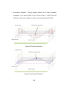
5-9. Tx power vs RSL for 2.4 GHz. ................................................................. 123
5-10. Path loss vs transmission distance. ......................................................... 130
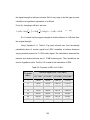
6-1. Field survey data...................................................................................... 142
6-2. Overlapping and non overlapping channels. ............................................ 148
6-3. Input parameters for modeling. ................................................................ 155
6-4. Output parameters obtained after simulation. .......................................... 156
6-5. Nanostaion2 configuration settings. ......................................................... 160
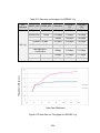
8-1. Bandwidth vs throughput.......................................................................... 194
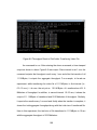
8-2. A typical example of an Iperf outputted result window. ............................ 196
8-3. Iperf arguments and their purposes. ........................................................ 197
8-4. Throughput Expt. 8.2.1-1: Parameters settings........................................ 209
8-5. Throughput Expt. 8.2.1-2: Parameters settings........................................ 210
8-6. Throughput Expt. 8.2.1-3: Parameters settings........................................ 211
8-7. Throughput Expt. 8.2.1-4: Parameters settings........................................ 212
8-8. Throughput Expt. 8.2.2-1: Parameters settings........................................ 215
8-9. Throughput Expt. 8.2.2-2: Parameters settings........................................ 216
8-10. Throughput Expt. 8.2.2-3: Parameters settings........................................ 217
x
8-11. Throughput Expt. 8.2.2-4: Parameters settings........................................ 218
8-12. Throughput results of Iperf and network speed tool. ................................ 219
8-13. Data rate vs throughput for IEEE802.11g. ............................................... 224
xi
LIST OF ILLUSTRATIONS
Page
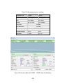
2-1. Greenbelt Weather Station (GBC_WS)........................................................ 8
2-2. Environmental Monitoring System in Greenbelt Corridor ............................. 8
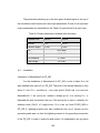
2-3. Discovery Park Weather and Soil Station (DP_WS) .................................. 10
2-4. Environmental Monitoring System in Discovery Park................................. 11
3-1. Dataloggers Used in the Field .................................................................... 14
3-2. Wiring Panel of CR10X .............................................................................. 15
3-3. Wiring Panel of CR1000 ............................................................................ 20
3-4. 03001 RM Young Wind Sentry................................................................... 24
3-5. Air Temperature and RH Sensor and Radiation Shield .............................. 26
3-6. CS106 and Its Jumper Setting ................................................................... 27
3-7. LI200X Pyranometer .................................................................................. 29
3-8. TE525 Tipping Bucket Rain Gage.............................................................. 30
3-9. EC-5 Soil Moisture Sensor ......................................................................... 32
3-10. T4 Tensiometer .......................................................................................... 34
3-11. 12 V 12 Ahr Sealed Lead Acid Rechargeable Battery ............................... 36
3-12. Solar Panels............................................................................................... 38
3-13. Charging Regulator Circuit Diagram .......................................................... 40
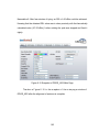
3-14. SC32B Optically Isolated RS-232 Interface ............................................... 42
3-15. Nanostation2 .............................................................................................. 44
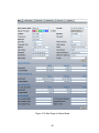
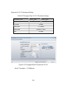
3-16. Main Page in Station Mode ........................................................................ 48
xii
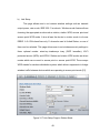
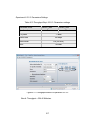
3-17. Link Setup Page in Station Mode ............................................................... 49
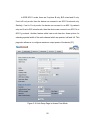
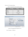
3-18. Link Setup Page in Access Point Mode ..................................................... 50
3-19. Network Page in Bridge Mode ................................................................... 51
3-20. Network Page in Router Mode ................................................................... 52
3-21. Advanced Page in Conservative Rate Algorithm Mode ............................. 54
3-22. Services Page ............................................................................................ 56
3-23. System Page.............................................................................................. 58
3-24. NL120 ........................................................................................................ 59
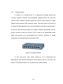
3-25. Network Switch .......................................................................................... 60
4-1. Functional Overview: Greenbelt Weather Station (GBC_WS) ................... 62
4-2. PC208W Main Window .............................................................................. 64
4-3. .CSI Input Program File ............................................................................. 68
4-4. Edlog .DLD Program File ........................................................................... 69
4-5. Edlog .FSL Program File ............................................................................ 70
4-6. ASCII, Comma Separated Input File .......................................................... 71
4-7. ASCII-Printable Input File........................................................................... 71
4-8. Field Formatted ASCII Input File ................................................................ 72
4-9. Functional Overview of DP_WS ................................................................. 73
4-10. PC208W Main Window .............................................................................. 75
4-11. Transformer Utility: .CSI to .CR1 Input Files .............................................. 80
4-12. Transformer Utility: .CSI to .CR1 Output Files ........................................... 80
4-13. CRBasic .CR1 Input Program File ............................................................. 83
xiii
4-14. Normal View-Comma Separated ............................................................... 85
4-15. Expand Tabs View-Field Formatted ........................................................... 85
4-16. Hex View-Hexadecimal Format.................................................................. 86
4-17. Inter-connections of Radio Equipments of DP_WS.................................... 87
5-1. 2.4 GHz Wi-Fi Channels ............................................................................ 94
5-2. A Pictorial View of 2.4 GHz Technology Applications .............................. 102
5-3. Speed Vs Mobility: WLAN Technologies .................................................. 104
5-4. Electromagnetic Wave Propagation ......................................................... 108
5-5. Radio Waves: Direct Wave and Ground Reflected Wave ........................ 112
5-6. Radio Waves: Surface Wave and Sky Wave ........................................... 112
5-7. Ionospheric Refraction ............................................................................. 114
5-8. Vertical Polarization ................................................................................. 118
5-9. Horizontal Polarization ............................................................................. 118
5-10. Free Space Propagation Model ............................................................... 121
5-11. Tx Power Vs RSL for 2.4 GHz ................................................................. 124
5-12. Two-Ray Propagation Model.................................................................... 125
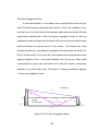
5-13. Path Loss Vs Transmission Distance ....................................................... 131
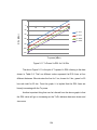
5-14. Attenuation Vs Distance ........................................................................... 133
6-1. EESAT – DP_WS .................................................................................... 137
6-2. Google Map Snapshot of EESAT – DP_WS Link .................................... 141
6-3. US 2.4 GHz Channel System................................................................... 147
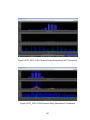
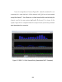
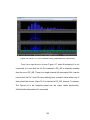
6-4. AirView2: A 2.4 GHz Wi-Fi Spectrum Analyzer ........................................ 149
xiv
6-5. DP_WS 2.4 GHz Channel Study (Nanostation2 NOT Connected) .......... 151
6-6. DP_WS 2.4 GHz Channel Study (Nanostation2 Connected) ................... 151
6-7. EESAT 2.4 GHz Channel Study (Nanostation2 NOT Connected) ........... 152
6-8. EESAT 2.4 GHz Channel Study (Nanostation2 Connected) .................... 153
6-9. Simulation Result of EESAT - DPWS Radio-link Modeling ...................... 155
6-10. Nanostations in EESAT and DP_WS ....................................................... 158
6-11. Antenna Radiation Pattern ....................................................................... 162
6-12. Snapshot of DPWS_NS2 Main Page ....................................................... 163
7-1. Disrupted Fresnel Zone ........................................................................... 169
7-2. Waste of Energy Due to Improper Antenna Adjustment .......................... 170
7-3. Vertical Tilting of Antenna ........................................................................ 171
7-4. Data Rate Vs Rx Sensitivity from Table 3-15 ........................................... 173
7-5. A 2.4 GHz North American Channel System ........................................... 176
7-6. Space Diversity Using Two Antennas in Receiver ................................... 180
7-7. 1st Fresnel Zone ....................................................................................... 183
7-8. Fresnel Zone being Obstructed in Various Ways ..................................... 184
7-9. Use of a Passive Repeater for Rerouting a LOS Blocked Signal ............. 190
7-10. Use of an Active Repeater to Retransmit the Weakened Signal .............. 190
8-1. Throughput Test Setup for Cat5 Cable .................................................... 198
8-2. Throughput Result of Cat5 while Transferring Video File ......................... 199
8-3. Throughput Test Setup for Wireless Router ............................................. 200
8-4. Throughput Result of Wireless Router while Transferring Video File ....... 201
xv
8-5. Throughput Test Setup for Nanostation2 ................................................. 202
8-6. Throughput Result of Experiment 1 ......................................................... 203
8-7. Throughput Result of Experiment 2 ......................................................... 204
8-8. Throughput Result of Experiment 3 ......................................................... 204
8-9. Throughput Result of Experiment 4 ......................................................... 205
8-10. Throughput Test Setup for EESAT_NS2-DPWS_NS2 Link ..................... 207
8-11. Throughput Result of Experiment 8.2.1-1 ................................................ 209
8-12. Throughput Result of Experiment 8.2.1-2 ................................................ 210
8-13. Throughput Result of Experiment 8.2.1-3 ................................................ 211
8-14. Throughput Result of Experiment 8.2.1-4 ................................................ 212
8-15. Throughput Result of Experiment 8.2.2-1 ................................................ 215
8-16. Throughput Result of Experiment 8.2.2-2 ................................................ 216
8-17. Throughput Result of Experiment 8.2.2-3 ................................................ 217
8-18. Throughput Result of Experiment 8.2.2-4 ................................................ 218
8-19. Data Rate Vs Throughput for IEEE802.11g ............................................. 224
xvi
LIST OF ACRONYMS
AAP
Adaptive antenna polarity
ASCII
American Standard Code for Information Interchange
BASIC
Beginner’s All-purpose Symbolic Instruction Code
Cat.5
Category 5
CCK
Complementary code keying
CDMA
Code division multiple access
CRI
Computing research infrastructure
DECT
Digital European cordless telephone
DHCP
Dynamic Host Control Protocol
DIFF
Differential
DP_WS
Discovery Park Weather Station
DPWS_NS2
Discovery Park Weather Station Nanostation2
DSSS
Direct sequence spread spectrum
EESAT
Environmental Education, Science and Technology
EESAT_NS2
Environmental Education, Science and Technology
Nanostation2
EHF
Extremely high frequency
ELF
Extremely low frequency
ESSID
Extended Service Set Identification
EWMA
Exponentially weighted moving average
xvii
FCC
Federal Communications Commission
FSL
Free space loss
GBC_WS
Greenbelt Corridor Weather Station
GPRS
General packet radio service
GPS
Global positioning system
GSM
Global system for mobile communications
HF
High frequency
Hi-Fi
High fidelity
HTTP
Hypertext Transfer Protocol
HTTPS
Hypertext Transfer Protocol Secure
ICMP
Internet Control Message Protocol
IEEE
Institute of Electrical and Electronics Engineers
IP
Internet Protocol
ISM
Industrial, scientific and medical
Kbps
Kilo bits per second
KBps
Kilo bytes per second
LAN
Local area network
LF
Low frequency
LOS
Line of sight
MAC
Media access control
Mbps
Mega bits per second
MBps
Mega bytes per second
xviii
NFC
Near field communication
NHC
Natural Heritage Center
OFDM
Orthogonal frequency division multiplexing
OSI
Open System Interconnection
PSD
Power spectral density
RH
Relative humidity
RSL
Receive signal level
RTMC
Real time monitor and control
RTMC-Dev
Real time monitor and control -Development
RTMC-RT
Real time monitor and control -Run Time
RTS
Request-to-send
SBC
Single board computer
SCADA
Supervisory control and data acquisition
SDI
Serial data interface
SE
Single ended
SHF
Super high frequency
SNMP
Simple Network Management Protocol
SNR
Signal-to-noise ratio
SSID
Service set identification
SWAP
Shared Wireless Access Protocol
TCP/IP
Transmission Control Protocol/Internet Protocol
UDP
User Datagram Protocol
xix
UHF
Ultra high frequency
UMTS
Universal mobile telecommunication system
UNT
University of North Texas
UTP
Unshielded twisted pair
UV
Ultraviolet
UWB
Ultra wide band
VHF
Very high frequency
VLF
Very low frequency
VWC
Volumetric water content
WDS
Wireless distribution system
WEP
Wired equivalent privacy
Wi-Fi
Wireless fidelity
WiMAX
Worldwide Interoperability for Microwave Access
WLAN
Wireless local area networking
WPA
Wi-Fi protected access
WRAN
Wireless regional area networks
xx
CHAPTER 1
INTRODUCTION
Real time environmental monitoring is the process of collecting
environmental data of a particular area by deploying an automated station where
different kinds of environmental sensors are connected. Environmental
parameters such as wind speed and wind direction, rainfall, solar radiation, air
pressure, air temperature, relative humidity etc. can be measured with the help of
those sensors deployed in the field.
The present thesis is based on the field work carried out at Greenbelt
Weather and Soil Station (GBC_WS hereafter) located at the Greenbelt Corridor
of the Ray Roberts State Park, Denton, and Discovery Park Weather and Soil
Station (DP_WS hereafter) at the University of North Texas (UNT hereafter),
Denton during January 2008 - October 2009. The thesis provides a
comprehensive description of the various steps involved, i.e., data collection, and
transfer of data. This work includes data collection procedure, transferring of data
from one data collection unit (datalogger) to another, and finally transmitting all
those combined collected data to a web server using wireless fidelity (Wi-Fi
hereafter) technology, where, once processed is made available for public
access via internet.
1
This thesis presents an al ternative method t o t he co stly general packe t
radio se rvice (GPRS hereafter) solution, wh ich has been used for tr ansmitting
data from the GBC_WS to the computing research infrastructure (CRI hereafter)
web server. An i nnovative, l ow co st and a hi gh dat a r ate Wi-Fi t echnology is
employed to t ransmit t he co llected dat a from t he w eather st ation i n the field t o
the web server. S ince the new W i-Fi t echnology replaces the G PRS network,
service charge doesn’t have to pay service charge for the new system deployed
in DP_WS, thus cutting down the cost of transmission. Wi-Fi technology operates
in an unlicensed frequency band and hence its use is free.
1.1
Objectives
•
Deploy a weather and so il monitoring sy stem t o collect env ironmental
data from the field
•
Improve t he data transmission quality o f se rvice by i mplementing a low
cost and high data rate unlicensed Wi-Fi technology
1.2
Hardware Description: (Background)
This section includes a brief description of the hardware components used
in t his work. An a utomated station deployed in a p articular ar ea collects
environmental d ata. A t ypical w eather st ation comprises various devices. A
datalogger is a programmable electronic device that records environmental data
from various kinds of environmental sensors. Its main functions are data
2
collection and storage. The datalogger used in this work is a product of Campbell
Scientific Inc.
Sensors, wired with the datalogger, are the other important components of
the station. They measure environmental parameters such as air temperature, air
pressure, w ind sp eed an d w ind d irection, rainfall, solar r adiation, relative
humidity, soil m oisture, etc. The remaining co mponents relate to p ower supply:
battery, solar panel, charging regulator etc. The datalogger, battery and charging
regulator are c ontained inside a
weatherproof enclosure, w hile all t he
environmental sensors and solar panel remain outside of the enclosure.
In or der t o transmit t he co llected da ta t o the s erver, a Wi-Fi lin k is
established usi ng a N anostation2, which is a radio equipment m anufactured by
Ubiquity Networks and operates at 2.4 GHz. It has a built-in directional antenna,
which radiates the si gnal i n l ine of si ght (LOS) direction. Two Nanostation2
devices were installed, one a t each si te. At th e weather st ation (data collection
site) and the base site (where there is an internet access). By linking these two
sites via Nanostation2 link, the data collected by weather station are sent to the
system server.
An ethernet i nterface allows connecting the datalogger and t he
Nanostation2. This interface allows the d atalogger t o co mmunicate over a l ocal
network
or a dedi
cated i nternet co nnection v ia
Protocol/Internet Protocol (TCP/IP here after) [1].
3
Transmission C ontrol
1.3
Motivation
Before the implementation of t his new Wi-Fi t echnology in the project,
GPRS n etwork has been use d and h ence has been pai d for i ts services to
transmit the data to the CRI web server. The pl an was to directly t ransmit t he
data f rom the field t o the server, and reduce co st substantially. In addi tion, the
typical data throughput of GPRS net work is around 15 -40 K bps while i ts
maximum d ata r ate i s 171.2 Kbps [2-4]. This is m uch l ower t han t he Wi-Fi
technology, which is being used now.
Wi-Fi technology fits both in quality transmission and in cost effectiveness
for the application that t his thesis talks about. With Wi-Fi t echnology, one ca n
achieve greater data throughput and radio-link stability; therefore this technology
is selected this for implementing the link at the DP_WS.
1.4
Contribution to the Field
Using the Wi-Fi t echnology resource, a high-speed radio lin k has been
established for t ransmitting t he environmental data f rom the f ield t o the server.
This avoids the n ecessity of paying for any third party f or usi ng t heir se rvices
such as GPRS n etwork. This thesis o ffers guidelines of the techniques to
implement similar ki nd o f pr ojects; f or example, developing wireless internet
service in remote and rural areas especially in developing countries.
4
1.5
Organization of the Thesis
Chapter 2 is an overview of weather monitoring system with its functional
block diagram. The o verview includes the two s ystems: the GBC_WS and the
DP_WS. However, the l atter is described i n more detail beca use t his thesis
focuses on this station for the implementation of Wi-Fi technology.
Chapter 3 de als with the detailed description of all the components of the
weather monitoring system with the wirings of all the sensors used in this project
and their core functions.
Chapter 4 deal s with t he da ta co llection pr ocedure from t he field. I n t his
chapter, a functional ov erview, datalogger support so ftware, and datalogger
programming are discussed.
Chapter 5 discusses W i-Fi t echnology, i ts advantages and ch allenges. I t
also describes radio wave pr opagation t heory f ocusing on t he free sp ace
propagation model and free sp ace l oss. This chapter al so di scusses some
advantages of Wi-Fi technology over GPRS technology for this application.
Chapter 6 de als with t he d etailed description o f the Wi-Fi link set up
between (Environmental E ducation, Science and T echnology (EESAT)) building
of the UNT and DP_WS. It also introduces radio-link modeling software used to
pre-assess t he link quality and
a W i-Fi spectrum-analyzer tool kn own as
AirView2 for choosing the appropriate channel.
Chapter 7 describes various techniques for Wi-Fi link quality optimization.
It also includes received power calculation, comparison of results using different
5
approaches such a s theoretical ca lculation, radio m obile so ftware and
Nanostation2 built in tool. Also di scussed i s the importance o f Fresnel z one
calculation for optimizing the link quality.
Chapter 8 deals with the various throughput tests using the Iperf tool and
Nanostation2 Network Speed tool, and analysis of their results. This chapter also
discusses some t echniques to i mprove t he throughput of t he l ink established
between DP_WS and EESAT.
Chapter 9 concludes the thesis with a summary and providing guidelines
for possible future extensions of this work.
6
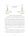
CHAPTER 2
WEATHER MONITORING SYSTEM: OVERVIEW
Work has been do ne i n two weather and so il monitoring systems
(GBC_WS and DP_WS). Each one consists of an environmental data collecting
electronic device known as
datalogger, environmental sensors, pow ering
equipments like bat tery, charging devi ce su ch as solar pan el an d a ch arging
regulator. The datalogger, pressure sensor, battery and ch arging r egulators are
inside an enclosure mounted on a tripod. Except the barometric pressure sensor,
all other environmental sensors and solar panels are outside the enclosure.
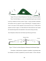
2.1
Environmental Monitoring System in Greenbelt Corridor (GBC_WS)
The GBC_WS is located in the m idst of the forest o f G reenbelt C orridor
State P ark situated at U S-380, D enton, T X-USA. The U NT E COPLEX pr oject
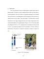
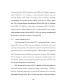
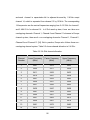
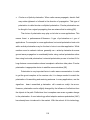
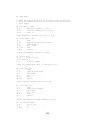
deployed the sy stem in 2004. Figure 2 -1 i s t he pi cture o f GBC_WS taken on
September 20 09. The m ain objective w as to m onitor different kinds of
environmental phenomena by m easuring different weather par ameters such a s
air t emperature, air p ressure, r elative hu midity, r ainfall, w ind sp eed a nd w ind
direction, s olar r adiation e tc and the s oil m oisture ar ound t he w eather st ation.
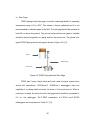
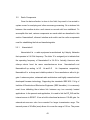
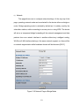
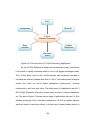
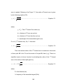
Figure 2
-2
shows
the
functional
7
block
diagram o
fG
BC_WS.
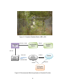
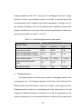
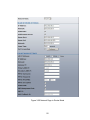
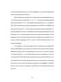
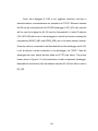
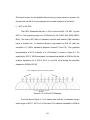
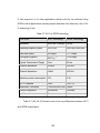
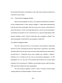
Figure 2-1 Greenbelt Weather Station (GBC_WS)
Gateway
SBC
RS 232 - CS I/O
Soil Moisture
Station
SDI-12
Weather
Station
RS-232
GPRS link
GPRS
Modem
GPRS
Network
Internet
Internet
900/1800 MHz
Internet
Internet
CRI System
Web Server
Figure 2-2 Environmental Monitoring System in Greenbelt Corridor
8
There ar e two systems in GBC_WS. O ne st ation m easures weather
parameters like air temperature, relative humidity, air pressure, wind speed and
direction, so lar r adiation, and rainfall. The other st ation i s for m easuring so il
moisture and soil pressure around the station. For the sake of simplicity, they will
be referred to as weather station and soil moisture station respectively.
There is a datalogger in each station for collecting and storing data. The
data are co llected at an i nterval o f 15 m inutes. The w eather st ation datalogger
and soil moisture datalogger connect by wire with each other and the program is
written in such a way that once the data are collected in both of the dataloggers,
the data of weather station are transferred to the soil m oisture station. A single
board computer (SBC hereafter) acts as an interface between the GBC weather
station and CRI web server. To be more specific, it acts as a bridge between the
datalogger and the GPRS modem. Then those collected data are transmitted to
GPRS net work via a G PRS modem, w hich operates at 900/1800 MHz. The
modem f orwards the data to t he CRI syst em w eb se rver where t hey a re
processed, refined and finally made accessible to public via internet.
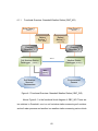
2.2
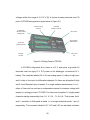
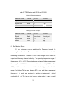
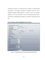
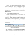
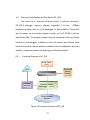
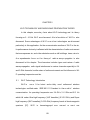
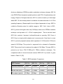
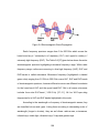
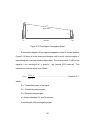
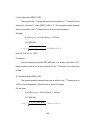
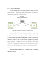
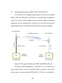
Environmental Monitoring System in Discovery Park
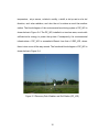
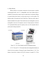
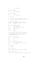
The D P_WS is located at Discovery P ark o f UNT situated i n Denton,
Texas, U SA. T he sy stem w as deployed i n October, 2008 by the CRI P roject
Team of UNT. Figure 2-3 is the picture of DP_WS taken on June 2009. The main
objective w as to set up a t
est b ed for t he pr oject as well as to monitor
environmental co nditions by m easuring di fferent w eather par ameters like air
9
temperature, air pr essure, r elative h umidity, r ainfall, w ind sp eed a nd w ind
direction, and solar r adiation; and also t he so il m oisture ar ound t he w eather
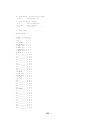
station. The block diagram of the environmental monitoring system of DP_WS is
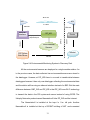
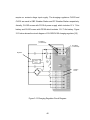
shown below in Figure 2-4. The DP_WS, installed in a tree-less area, counts with
sufficient so lar energy to power t he sy stem. C onsequently, t he environmental
infrastructure o f DP_WS is somewhat di fferent from that o f GBC_WS, where
there is tree cover all the way around. The functional block diagram of DP_WS is
shown below in Figure 2-4.
Figure 2-3 Discovery Park Weather and Soil Station (DP_WS)
10
Wi-Fi link
NS2
NS2
2.4 GHz
Ethernet
DP_WS
EESAT
Environmental
Sensors
CRI System
Web Server
Router
40-pin parallel
peripheral port
DPWS
Internet
Ethernet
Interface
Ethernet
Internet
Internet
Figure 2-4 Environmental Monitoring System in Discovery Park
All the environmental sensors are deployed in a single weather station. As
in the previous case, the data collected via environmental sensors are stored in
the datalogger. However, at D P_WS t here i s no ne ed to transfer data between
dataloggers because it has only one datalogger collecting the environmental data
and the station will be using an ethernet interface instead of a SBC. But the main
difference between GBC_WS and DP_WS is that DP_WS uses Wi-Fi technology
to transmit the data t o t he C RI system web server instead of using G PRS. The
Ubiquity Networks product named Nanostation2 links DP_WS and the internet.
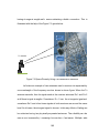
The Nanostation2 is installed at the top o f a 9 m tall pole. Another
Nanostation2 is installed at t he t op of EESAT building of UNT and co nnected
11
with an internet source. These t wo nanostations are i nstalled f acing each o ther
so that they are in a line of sight (LOS hereafter) as shown in above Figure 2.4.
Because the antenna inside the Nanostation2 is directional, the direct wave is the
one which i s of m atter of co ncern and so both o f the na nostations should be
visible to each other or in other words there should not be any obstruction in the
LOS pa th. The more detailed description of Nanostation2 is given in Chapter 3.
Once b oth of t he nanostations are i nstalled properly so t hat t hey l ie al ong t he
LOS pa th, the l ink could be est ablished a fter pow ering t hem and configuring
some settings. The detailed description of the link set up is given in Chapter 6.
12
CHAPTER 3
COMPONENTS OF ENVIRONMENTAL MONITORING SYSTEMS
The environmental monitoring system consists of various components. For
the pr esent w ork, these all co mponents fall under two di fferent categories: i)
weather st ation c omponents and ii) radio co mponents. This section co ntains a
description of all of these components.
3.1
Weather Station Components
3.1.1 Datalogger
A datalogger is an el ectronic programmable instrument or d evice t hat
records environmental data ov er t ime via i ts built i n or ex ternal sensors. It i s
generally powered by a lead acid rechargeable battery, which is recharged by an
AC adapter wherever available, and by a solar panel. Generally, they are small
and hence portable. It has an internal memory for data storage and is based on a
digital pr ocessor. Dataloggers come i n two t ypes. The f irst type o f dataloggers
needs a P C for activating, dow nloading so ftware, v iewing and a nalyzing t he
collected data. The second type of dataloggers has a local interface device and
can be used as a stand-alone device. Between the above-mentioned two t ypes
of dataloggers, the f irst type has been use d because t hese ar e appropriate f or
recording dat a automatically and c ontinuously f rom t he environment once
deployed and act ivated in the f ield. Campbell S cientific dataloggers of CR1 0X
13
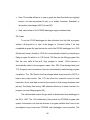
and C R1000 s eries are use d i n t his work. Pictures of t ypical CR10X and
CR1000 dataloggers are given below.
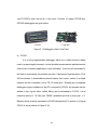
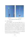
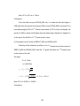
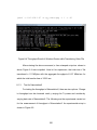
i) CR10X
ii) CR1000
Figure 3-1 Dataloggers Used in the Field
a) CR10X
It i s a fully pr ogrammable datalogger with a no n v olatile m emory widely
used in meteorological research, routine weather measurement applications and
other kinds of network applications. Upon activation, it can be left unattended in
the field to continuously record data over time. It performs a high-resolution 13-bit
A/D co nversion. A d etachable ke yboard di splay that can be carried to m ultiple
stations can b e co nnected v ia i ts CS I /O serial por t. Running any co mpatible
datalogger support software on the PC connected to CR10X, the program can be
written i n a pr ogram editor called Edlog and d ownloaded t o C R10X. It h as
internal m emory of 12 8 Kb ytes SRAM (available opt ional m emory up t o 2
Mbytes) which is nearly equivalent to 60,000 data points [5]. A picture of a typical
CR10X is shown above in Figure 3-1(i).
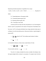
14
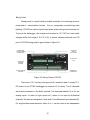
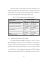
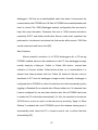
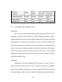
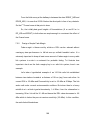
Wiring Panel
Wiring panel is a panel which provides terminals for connecting sensors,
power and co mmunication d evices. It al so i ncorporates protection ag ainst
lightning. CR10X has various input/output ports, power and ground terminals etc.
To power the datalogger, the voltage level required is 12 V DC but it can intake
voltages within the r ange of 9.6-16 V [5]. A picture showing t erminals and I/O
ports of CR10X wiring panel is given below in Figure 3-2.
6 Differential
(12 single-ended)
Analog Inputs
Power and
Ground
Connections
9-pin CS I/O
Port
3 Switched
Excitation
Channels
8 Digital I/O
(Control) Port
2 Pulse Counting
Channels
Figure 3-2 Wiring Panel of CR10X
There are a 12 V and a power ground (G) terminals used to supply 12 V
DC pow er t o t he C R10X datalogger via external 1 2 V b attery. The G t erminals
are directly connected to the Earth terminal. The terminals labeled 1H to 6L are
analog i nputs. H r efers to high i nput a nd L r efers to l ow i nput for di fferential
channels. So there are altogether 6 high and 6 low differential input channels [5].
For si ngle-ended m easurements, either H or L can b e used as an i ndependent
15
channel to measure voltage with respect to AG (Analog Ground) of CR10X. So
there are altogether 12 single-ended channels starting sequentially from 1H, 1L,
2H,...5L, 6H, 6L. That means the H and L t erminals of differential channel 1 ar e
single-ended channels 1 and 2 respectively. The t erminals labeled E 1, E 2 and
E3 ar e sw itched ex citation ou tputs used to su pply pr ogrammable ex citation
voltages for r esistive bridge m easurements. The t erminals P1 an d P2 are t he
pulse co unter ch annels. T erminals labeled as C1, C 2,….,C8 a re t he di gital
input/output ports. They are also called control ports. There are two 5 V outputs
used t o pow er so me ex ternal se nsors that r equire 5 V pow er su pply. The
switched 12 V outputs can be used to power sensors and devices which require
an unregulated 12 V. There is one 9-pin serial I/O port used for communication
between CR10X and external devices such as PC, printers and other compatible
serial devices [5].
CR10X Operating Systems
The default op erating sy stem l oaded on CR10X i s the Array-Based
Operating System unless another is specified at the time of ordering it. Available
operating systems for CR10X are:
•
Mixed-array oper ating s ystem ( standard): Contains 48 m easurement
instructions, 52 processing/math i nstructions, an d 2 0 pr ogram co ntrol
instructions [5].
16
•
Table data o perating sy stem (OS10XTD/U): A llows the C R10X t o st ore the
final storage data in the form of a table [5].
•
PakBus table da ta o perating sy stem (OS10XPB/U). A llows the C R10X t o
communicate w ith C R200-series dataloggers in t he s ame n etwork. F inal
storage data are stored in table format [5].
•
Modbus operating system (OS10XMB/U): Supports Modbus protocol allowing
the CR10X to interface with supervisory control and data acquisition (SCADA)
and MMI software packages. Some earlier CR10X operating systems (OS10X
versions older than 1.3) included Modbus in the standard operating systems
[5].
•
OS10X A LERT operating sy stem: A llows the C R10X t o st ore and t ransmit
data in the ALERT format (flood warning system) [5].
SDI-12
SDI-12 i s the acr onym f or “ serial dat a i nterface at 12 00 baud” It i s a
standard c ommunication protocol al lowing co nnection o f m ultiple se nsors to an
SDI-12 compatible datalogger. SDI-12 sensors connect to control ports C1–C8 of
CR10X. It communicates using a cable containing 3 wires; a 12 V line, a ground
line an d a s erial dat a line [5]. SDI-12 c an also be used t o c onnect t wo C R10X
dataloggers for making it possible to communicate between the two dataloggers.
Once they are co nnected v ia S DI-12 i nterface, t he pr ogram transfer, d ata
transfer etc. between them is possible.
17
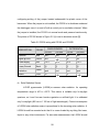
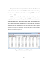
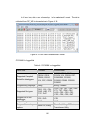
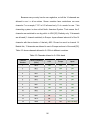
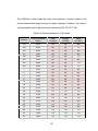
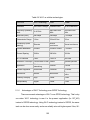
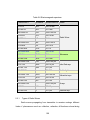
Table 3-1 CR10X technical specifications.
FEATURE
SPECIFICATION
Voltage
9.6 - 16 Vdc (optimum 12 V)
Current drain
Quiescent - 1.3 mA
Processing - 13 mA
Active - 46 mA
Analog inputs
12 Single Ended, 6 Differential
Digital/Control ports
8 I/Os (C1 - C8)
Pulse Counter channel
2 (P1, P2)
Communication port
1 CS I/O
Data Storage
Internal memory - 128 Kbytes SRAM
(available up to 2 Mbytes)
Input Voltage range
±2.5 V
Switched voltage output
two 12 V
Other voltage output
two 5 V and two 12 V
Scan rate
64 Hz
A/D conversion
13-bits
Switched volt excitation channel
3 (E1, E2 & E3)
Programming
Edlog
Datalogger support software
PC208W, LoggerNet 2.x, PC400
Operating systems
Mixed Array, Table, PakBus, Modbus,
ALERT
Communication protocol
Modbus, ALERT
Standard Temperature Range
-25ºC - +50ºC
Dimension
7.8” × 3.5” × 1.5”
Weight
2 lbs
18
b) CR1000
Like CR10X, it is also a fully programmable datalogger with a non v olatile
memory. I t i s a new pr oduct o f C ampbell S cientific Inc. d esigned especially f or
replacing t he ol d C R10X t o add , upg rade a nd i mprove so me of t he features of
CR10X. I t is
also widely use d i n m eteorological r esearch, r outine w eather
measurement ap plications and ot her ki nds of network applications. I t is also
designed for unattended network applications.
It has a high-resolution 13-bit A /D c onversion with higher sp eed o f scan
rate of 100 Hz. CR1000 is compatible with various datalogger support software
like LoggerNet3.x. PC400 1.2, ShortCut 2.2 etc. The program can be written and
compiled in a program editor called CRBasic. Facilitating more storage, it has an
internal memory of 2 Mbytes SRAM and available optional memory extends up to
4 Mbytes. Instead of ±2.5 V, it has ±5 V input range allowing the sensors output
of 5 V without the use of voltage divider. For communication with other external
devices, in addi tion t o C S I /O se rial p ort, it also offers two other additional
different ports; an RS-232 serial por t and a 40-pin parallel p eripheral p ort.
CR1000 c omes up w ith pr ocessing sp eed 4 t imes faster t han t hat of r etired
CR10X [6]. A picture of a typical CR1000 is shown above in Figure 3-1(ii).
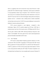
Wiring Panel
CR1000 has various input/output por ts, pow er and g round t erminals etc.
To p ower t he datalogger, the voltage r equired i s 12 V D C but i t ca n intake
19
voltages within t he r ange of 9. 6-16 V [6]. A pi cture sh owing t erminals and I /O
ports of CR1000 wiring panel is given below in Figure 3-3.
2 pulse counting
channels
3 switched
excitation channels
8 Differential
(16 single-ended)
Analog inputs
RS-232 port
40-pin Parallel
peripheral port
Power and
ground terminals
8 Digital
I/O ports
9-pin CS I/O
port
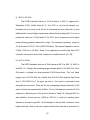
Figure 3-3 Wiring Panel of CR1000
In C R1000 w iring panel al so, t here is a 12 V and a pow er g round ( G)
terminals used t o s upply 12 V D C p ower t o t he datalogger via ex ternal 12 V
battery. The terminals labeled 1H to 8L are analog inputs. H refers to high input
and L r efers to low input for differential channels. So there are altogether 8 hi gh
and 8 low di fferential input ch annels. F or si ngle-ended m easurements, H or L,
either of them can be used as an independent channel to measure voltage with
respect t o analog g round o f C R1000. S o t here ar e al together 1 6 single-ended
channels starting se quentially f rom 1H, 1 L, 2 H,...7L, 8 H, 8L. T hat m eans the H
and L t erminals of di fferential ch annel 1 a re si ngle-ended ch annels 1 an d 2
respectively. T he t erminals labeled V X1, V X2 and V X3 ar e sw itched excitation
20
outputs used t o s upply pr ogrammable ex citation v oltages for r esistive br idge
measurements. P 1 a nd P 2 t erminals are t he pul se co unter ch annels. T hey are
also called control ports. There is one 5 V output used to power some external
sensors that require 5 V power supply. The switched 12 V outputs can be used to
power se nsors and dev ices which r equire an u
nregulated 12 V
. For
communication b etween C R1000 a nd i ts external dev ices such a s PC, pr inters
and ot her co mpatible se rial and par allel d evices, t he CR1000 wiring panel i s
incorporated with a 9-pin serial CS I/O, an RS-232 port and a parallel peripheral
port. The peripheral port here can be used to connect Ethernet devices such as
NL115. Terminals labeled as C1, C2,….,C8 are the digital input/output ports. In
addition to communicating via its RS-232 and CS I/O ports, the CR1000 can also
communicate via the digital I/O COM ports [6].
CR1000 Operating Systems
The de fault operating sy stem l oaded o n C R1000 is PakBus Operating
System unless another is specified at the time of ordering it. Available operating
systems for CR1000 are:
•
PakBus table d ata operating sy stem: This operating sy stem use s a pack et
based communication which creates final storage tables to logically separate
different types of data collection such as hourly, daily etc. This protocol allows
the C R1000 to co mmunicate w ith other C R1000 dataloggers in t he sa me
network [6].
21
•
Modbus operating system: This operating system s upports Modbus protocol
(one o f t he m ore pr imitive pr otocols) allowing t he CR1 000 to i nterface w ith
SCADA an d M MI so ftware packa ges. It allows the r emote s etting o f co ntrol
ports and reading/changing of memory locations [6].
SDI-12
SDI-12 i s the acr onym f or “ serial dat a i nterface at 12 00 baud” It i s a
standard communication pr otocol allowing co nnection o f m ultiple sensors to an
SDI-12 compatible datalogger. SDI-12 sensors connect to control ports C1, C3 ,
C5 and C7 of CR1000. It communicates using a cable containing 3 wires; a 12 V
line, a ground line and a serial data line [6].
22
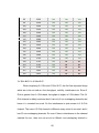
Table 3-2 CR1000 technical specifications.
FEATURE
SPECIFICATION
Voltage
9.6 - 16 Vdc (optimum 12 V)
Current drain
0.6 mA (Sleep mode)
1-16 mA (w/o RS-232 comm.)
17-28 mA (w/RS-232 comm.)
Analog inputs
16 Single Ended, 8 Differential
Digital/Control ports
8 I/Os (C1 - C8) or 4 RS-232 COM
Pulse Counter channel
2 (P1, P2)
Communication port
1 CS I/O, 1 RS-232,
1 parallel peripheral port
Data Storage
Internal memory - 2 Mbytes SRAM
(available up to 4 Mbytes)
Input Voltage range
±5.0 V
Switched voltage output
one 12 V
Other output voltage
one 5 V and two 12 V
Scan rate
100 Hz
A/D conversion
13-bits
Switched volt excitation channel
3 (VX1, VX2, VX3)
Programming
CRBasic
Datalogger support software
LoggerNet 3.4.x, PC400, etc.
Operating system
PakBus
Communication protocol
PakBus
Standard Temperature Range
-25ºC - +50ºC
Dimension
9.4” × 4.0” × 2.4”
Weight
2.1 lbs
23
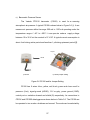
3.1.2
Environmental Sensors
Environmental se nsors are t he el ectronic components to measure
physical q uantities of environment su ch as light i ntensity, ai r t emperature, so il
moisture et c. and c onvert them i nto si gnals that ca n b e easi ly r ead by an
observer. There ar e many environmental sensors used f or m easuring different
environmental ph enomena, b ut only some o f them are used in t his project and
discussed here in this section.
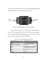
a) Wind Speed and Direction Sensor
For measuring wind speed and wind direction, 03001 RM Young Sentry is
used. A typical 03001 RM Young Sentry is shown in below Figure 3-4. It can be
mounted directly to the mast or to the cross arm as shown in above figure. It can
measure the wind speed within the range of 0-112 mph and wind direction 360º
mechanical a nd 355º electrical. The t emperature r ange w ithin w hich i t ca n
operate is -50º to +50ºC [7].
Wind vane
(for wind direction)
Wind cups
(for wind speed)
Crossarm
Figure 3-4 03001 RM Young Wind Sentry
24
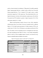
Wind sp eed sensor has 3 w ires: black, w hite and cl ear used f or wind
speed si gnal, wind speed r eference a nd w ind sp eed sh ield r espectively.
Similarly, wind di rection has 4 w ires: red, bl ack, white and cl ear used f or wind
directional si gnal, w ind di rection ex citation, w ind di rection r eference an d w ind
direction sh ield r espectively. The co nnections of t he se nsor t o C R10X and
CR1000 dataloggers are shown below in Table 3-3 [7].
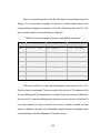
Table 3-3 03001 wiring with CR10X and CR1000.
Wind Speed
Wind
Direction
WIRE
COLOR
DESCRIPTION
CR10X
CR1000
Black
Wind speed signal
Pulse
Pulse
White
Wind speed reference
G
Clear
Wind speed shield
G
Red
Wind direction signal
SE Analog
SE Analog
Black
Wind direction excitation
Excitation
Excitation
White
Wind direction reference
AG
Clear
Wind direction shield
G
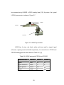
b) Air Temperature and Relative Humidity Sensor
The Vaisala temperature an d r elative hu midity (RH her eafter) sensor
(HMP50) is used for measuring air temperature. A typical HMP50 is shown below
in F igure 3 -5 (i). When i t i s i nstalled outdoor or ex posed i n su nlight, i t must be
housed in a solar radiation shield which can be mounted directly to the tripod or
tower mast as shown i n abov e Figure 3-5 ( ii). I t ca n m easure ai r t emperature
within the range -25º to +60ºC and relative humidity within the range of 0 to 98%.
25
The typical supply voltage is 12 V but it can intake any voltage within the range of
7 to 28 V DC. And typical current consumption is as low as 2 mA [8].
Tripod/tower
mast
Solar radiation
shield
HMP50
i) HMP50
ii) 41303 6-plate Gill Solar
Radiation Shield
Figure 3-5 Air Temperature and RH Sensor and Radiation Shield
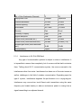
HMP50 has
5 w ires: black, w hite, b lue, brown and c lear used f or
temperature, r elative humidity, si gnal and power r eference, power and s hield
respectively. I ts connections t o C R10X an d C R1000 dataloggers are s hown
below in Table 3-4 [8].
Table 3-4 HMP50 wiring with CR10X and CR1000.
DESCRIPTION
COLOR
CR10X
CR1000
Temperature
Black
SE3
SE1
Relative Humidity
White
SE4
SE2
Signal and power reference
Blue
G
G
Power
Brown
12 V
12 V
Shield
Clear
G
26
c) Barometric Pressure Sensor
The Vaisala PTB110 barometer (CS106) is used for m easuring
atmospheric air pressure. A typical CS106 is shown below in Figure 3-6 (i). It can
measure air pressure within the range 500 m b to 1100 m b operating under t he
temperature r ange o f -40º t o + 60ºC. I t ca n oper ate under a supply v oltage
between 10 to 30 V but the nominal is 12 V DC. A typical current consumption is
about 4 mA during active period and less than 1 µA during quiescent period [9].
Jumper
CS106
i) CS106
i) CS106 jumper setting
Figure 3-6 CS106 and Its Jumper Setting
CS106 has 6 wires: blue, y ellow, r ed, bl ack, g reen an d cl ear used f or
pressure (Vout), signal g round (AGND), 12 V su pply, power ground ( GND),
control port or excitation channel and shield (G) respectively. Its connections to
CR10X and CR1000 dataloggers are shown below in Table 3-5. The CS106 can
be operated in two modes: shutdown and normal. The mode can be selected by
27
configuring se tting of the j umper l ocated underneath t he pl astic cover of t he
barometer. When the jumper is not installed, the CS106 is in shutdown mode and
the datalogger turns it on and off with a c ontrol port or excitation channel. When
the jumper is installed, the CS106 is in normal mode and powered continuously.
The picture of CS106 shown in Figure 3-5 (ii) is set to shutdown mode [9].
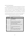
Table 3-5 CS106 wiring with CR10X and CR1000.
DESCRIPTION
COLOR
Pressure
SINGLE-ENDED
DIFFERENTIAL
CR10X
CR1000
CR10X
CR1000
Blue
SE7
SE7
4H
4H
Signal ground
Yellow
AG
4L
4L
Power supply
Red
12 V
12 V
12 V
12 V
Power Ground
Control or
Excitation
Black
G
Control
port
G
Control
port
G
Control
port
G
Control
port
Shield
Clear
Green
G
G
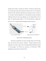
d) Solar Radiation Sensor
LI-COR pyranometer (LI200X) m easures solar r adiation. Its operating
temperature r ange is -40º t o + 65ºC. This sensor is suitable o nly f or day light
spectrum, so i t ca n’t be use d un der v egetation or ar tificial l ight. I t i s calibrated
only for daylight (400 nm to 1100 nm of light wavelength). Current consumption
of LI200X solar radiation sensor is proportional to the incoming solar radiation. A.
LI200X sh ould b e mounted su ch that i t i s never sh aded by anything l ike t ower,
tripod or any ot her i nstruments. For accu rate m easurement, t he L I200X sh ould
28
be m ounted usi ng LI2003S Li-COR leveling base [10]. A pi cture o f a t ypical
LI200X pyranometer is shown in Figure 3-7.
LI200X
LI2003S
Crossarm
Figure 3-7 LI200X Pyranometer
LI200X has 4 wires: red, bl ack, white and cl ear used f or signal, si gnal
reference, signal ground and shield respectively. Its connections to CR10X and
CR1000 dataloggers are shown below in Table 3-6 [11].
Table 3-6 LI200X wiring with CR10X and CR1000.
DESCRIPTION
COLOR
CR10X
CR1000
Signal
Red
1H
1H
Signal reference
Black
1L
1L
Signal ground
White
AG
Shield
Clear
G
29
e) Rain Gage
TE525 tipping bucket rain gage is used for measuring rainfall. Its operating
temperature r ange is 0º t o 50ºC. This sensor i s factory calibrated and it is not
recommended to calibrate again in the field. The rain gage should be mounted at
least 30 c m above the ground. The ground surface where rain gage is installed
should be na tural vegetation or gravel and not the paved one. The picture of a
typical TE525 tipping bucket rain gage is shown in Figure 3-8 [11].
TE525
Mounting pole
Ground level
Figure 3-8 TE525 Tipping Bucket Rain Gage
TE525 has 3 wires: black, w hite and cl ear used for si gnal, si gnal r eturn
and sh ield respectively. CR10X and C R1000 bot h dataloggers have t he
capability of co unting switch cl osures on so me o f t heir co ntrol po rts. When a
control port is used, the return from the rain gage switch should be connected to
5 V on t he datalogger. The T E525 connections to C R10X and C R1000
dataloggers are shown below in Table 3-7 [11].
30
Table 3-7 TE525 wiring with CR10X and CR1000.
i) Wiring for Pulse channel input
DESCRIPTION
COLOR
CR10X
CR1000
Signal
Black
Pulse channel
Pulse channel
Signal return
White
G
Shield
Clear
G
ii) Wiring for Control port input
f)
DESCRIPTION
COLOR
CR10X
CR1000
Signal
Black
Control port
Control port
Signal return
White
5V
5V
Shield
Clear
G
Soil Moisture Sensor
EC-5 soil moisture se nsor, m anufactured by D ecagon, is used for
measuring the so il moisture. The se nsor o btains volumetric water content by
measuring t he dielectric constant o f t he m edia t hrough t he ut ilization o f
capacitance/frequency domain t echnology. The operating t emperature r ange of
the sensor is -40º to +60ºC. The pointed prong design and hi gher measurement
frequency allows the EC-5 to measure volumetric water content (VWC) from 0 to
100%, and allows accurate measurement of almost all soil types and much wider
range o f sa linities. That m eans because E C-5 runs at hi gher m easurement
frequency, it
is much l ess sensitive t o variation i n t exture and el ectrical
conductivity of s oil The t wo poi nted prongs design m ake i t easy t o i nstall
31
anywhere even in hard or compact soil. However, it is better to insert the probe
very ca refully and g ently while i nserting i nto har d su rface so il. Also t he pr obe
should b e b uried co mpletely i nside t he g round s urface as sh own i n F igure 3 -9
(ii). The sensor is factory calibrated but it is recommended to perform soil specific
calibration because the f actory pre-calibration may not be appl icable f or al l soil
types. The nominal s upply v oltage i s 3 V DC but c an i ntake any voltage v alue
from 2.5 to 3.6 V. A typical current consumption is about 10 mA [12].
Ground level
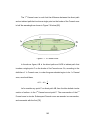
EC-5 prong
i) EC-5 Soil Moisture Sensor
ii) Inserting EC-5 probe inside ground
Figure 3-9 EC-5 Soil Moisture Sensor
The picture of a typical EC-5 is shown in the above Figure 3-9. EC-5 has 3
wires: red, w hite and cl ear used f or analog out , excitation signal and s hield
respectively. The sensor output is fed to the single ended (SE hereafter) channel
of t he da talogger. The EC-5 pr obe connections to C R10X and C R1000
dataloggers are shown below in Table 3-9 [12].
32
Table 3-8 EC-5 wiring with CR10X and CR1000.
DESCRIPTION
COLOR
CR10X
CR1000
Analog out
Red
SE1
SE1
Excitation channel
White
E1
VX1
Shield
Clear
G
EC-5 Calibration
Even though the EC-5 probes come with pre-calibrated for most soil types,
it is highly recommended that customers do perform re-calibration for specific soil
types. Since the ca libration equation v aries with t he so il t ypes, appropriate
calibration equation for sp ecific soil t ype should be use d. Following ar e t he
calibration equations for three different so il types (mineral soil, potting so il, and
rockwool) for the probes excited at 2500 mV [12].
VWC = 11.9 × 10 −4 × mV − 0.401
………………………………
Mineral soils
VWC = 10.3 × 10 −4 × mV − 0.334
……………………………….
Potting soils
VWC = 2.63 × 10 −6 × mV 2 + 5.07 × 10 −4 − 0.0394
……………..….
where,
VWC – volumetric water content of the soil
mV - output of the probe excited at 2500 mV [12].
33
Rockwool
g) Tensiometers
The T4 Tensiometer is used for measuring the soil water tension and soil
water pressure. The sensor is factory calibrated with an offset of 0 kPa (when in
horizontal posi tion). Since t he offset o f t he pressure t ransducer h as a minimal
drift over the years, it is recommended to check the sensors once a year and recalibrate t hem ev ery t wo years. The out put si gnal of T4 t ensiometer i s directly
dependent on t he su pply v oltage and h ence t he su pply v oltage nee ds to b e
constant and stabilized. The typical supply voltage is 10.6 V DC but can intake
any voltage value from 5 to 15 V. A typical current consumption is about 1.3 mA
at 10 .6 V . The measuring r ange of t he T4 t ensiometer i s -85 kP a t o 0 kP a of
water t ension. The picture o f a t ypical T4 t ensiometer is shown i n F igure 3 -10
[13].
Reference air
pressure
Cable gland
Ceramic cup
ii) T4 deployed in field
i) T4 segments
Figure 3-10 T4 Tensiometer
34
T4 T ensiometer has 5 wires: brown, white, bl ue, bl ack and t hick bl ack
used for supply+, signal+, supply-, signal- and shield respectively. This means it
uses DIFF ch annel o f t he dat alogger. The TE525 co nnections to C R10X and
CR1000 dataloggers are shown below in Table 3-9 [13].
Table 3-9 T4 wiring with CR10X and CR1000.
3.1.3
DESCRIPTION
COLOR
CR10X
CR1000
Supply+
Brown
5V
5V
Signal+
White
1H
1H
Supply-
Blue
AG
Signal-
Black
1L
1L
Shield
Thick black
G
G
Powering and Charging Devices
In order to perform any desired operation, an electrical power is required
for all systems that consist of electrical and electronic devices. In addition to that,
the power sy stem i s always expected to f unction well and i ts gravity i s even
higher in the system applications such as mobile services and etc. where even a
few se conds o f pow er failure i s no t t olerable. Depending u pon t he t ype of
application, the components of a power system vary. The power system for this
work is co mposed of battery backu p, so lar panel and ch arging r egulator. Other
elements such as AC pow er, pow er su pply adapters etc are al so di scussed in
this section.
35
a) Battery Backup
Battery backup i s an important component of pow er sy stem i n w eather
monitoring appl ication and it i s indispensable when t he w eather st ation i s
installed in an area such as desert, forest etc. where there’s no electricity. Battery
is a power backup when there’s no o ther power so urce t o r un t he system. The
batteries used i n this project ar e from P ower S onic. There ar e various types of
batteries available in the market. Some batteries are non-rechargeable, some are
rechargeable, some are of low capacity, some are of high capacity etc. Selection
of an appropriate battery type and capacity is also one of the important tasks in
power system design perspective.
+ve terminal
-ve terminal
ii) Battery installation inside
enclosure
i) PS-12120
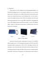
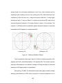
Figure 3-11 12 V 12 Ahr Sealed Lead Acid Rechargeable Battery
A 12 V 7 Ahr and 12 V 12 Ahr sealed lead acid rechargeable batteries are
chosen for the two stations in Greenbelt Corridor Weather Station. A 12 V 7 Ahr
battery of sa me ki nd i s chosen for DP_WS. A picture o f a typical 12 V 12 A hr
36
sealed lead acid rechargeable battery (PS-12120) is shown in above Figure 3-11.
It should be always connected to charging source through a charging regulator.
In this work, battery is connected to solar panel through a charging regulator in
every weather station. So in the day time when there’s sunlight, it is charged by
the so lar pan el and i t supplies power to the sy stem d uring w hole ni ght. But o f
course it should be charged enough in the daytime in order to supply power for
whole night.
The battery should be f ully ch arged be fore deploying i n t he field. Due to
self-discharge characteristics of this type of battery, it is required to charge them
after 6-9 months of storage, otherwise permanent loss of capacity might occur as
a result of sulfation [14]. Some technical specifications of the battery (PS-12120)
are given below in Table 3-10 [14].
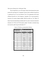
Table 3-10 Technical specifications of PS-12120.
DESCRIPTION
SPECIFICATIONS
Name
PS-12120
Nominal Voltage
12 V
Nominal Capacity
12 Ahr
Max.Discharge current (≤ 7 min.)
36 Amp.
Max. short duration Discharge
current (≤ 10 sec.)
120 Amp.
Approximate weight
3.86 kg
Operating temperature range
-20ºC to +50ºC
37
b) Solar Panel
Solar panel is one of the charging sources for rechargeable batteries. It is
an ess ential c harging so urce for t hose sy stems which ar e s et up i n a n ar ea
where source o f electricity is not av ailable. Solar pa nel is a ph otovoltaic power
source t hat converts solar ener gy i nto el ectrical ener gy. In ot her w ords, i t
converts the sunlight into direct current. Solar panel operates in both direct and
diffuse light (cloudy days), but not at night. MSX10 and SX-20 U solar panels are
used i n G BC Weather S tation an d S P20 so lar panel i s used i n D P Weather
Station. Figure 3 -12 below sh ows the p ictures o f different ki nds of the so lar
panels used in this project.
i) MSX10
ii) SX-20 U
iii) SP-20
Figure 3-12 Solar Panels
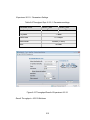
Among the three so lar panel s shown above in F igure 3 -12, t he M SX10
delivers a peak power of 10 W whereas the remaining two SX-20 U and SP-20
solar pa nels deliver a peak pow er o f 20 W [15-17]. Like battery, se lection of a
solar panel is also an important task. Solar panel should be chosen such that it
can charge the battery enough even within a short interval of sunlight especially
during w inter, r ainy day s and foggy day s etc. Solar pa nels connect di rectly t o
38
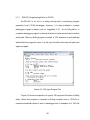
charging regulator w hose 1 2 V output g oes to datalogger input pow er supply
terminal. In or der to g et maximum amount of su nlight, s olar pa nel sh ould be
mounted facing south if located in the northern hemisphere or facing nor th if in
the southern hemisphere. Also t he t ilt angle sh ould b e a djusted correctly which
makes a lot difference in the output. Other technical specifications of these solar
panels are given below in Table 3-11 [15-17].
Table 3-11 Technical specifications of solar panels.
DESCRIPTION
SPECIFICATIONS
MSX10
SX-20 U
SP-20
Output power (peak)
10 W
20 W
20 W
Output Voltage (peak) (voltage
from solar panel before regulator)
17.5 V
16.8 V
17.1 V
Output current (peak)
0.57 Amp.
1.19 Amp.
1.17 Amp.
Guaranteed minimum peak
power
9W
18 W
18 W
Approximate weight
1.5 kg
3 kg
2.95 kg
c) Charging Regulator
A charging regulator must be used to connect rechargeable batteries with
a ch arging so urce. The ch arging r egulator co ntrols the c urrent flowing t o t he
battery and pr events the ba ttery cu rrent f rom flowing t o t he charging source.
Charging r egulator intakes an u nregulated pow er f rom solar pan el or A C wall
charger and charges the battery connected to it as well as supply power to t he
system simultaneously. It is an essential element for almost all the systems that
39
require a c onstant v oltage input su pply. The ch arging r egulators CH12R and
CH100 are used in GBC Weather Station and DP Weather Station respectively.
Actually, C H12R co mes with P S12LA p ower su pply which i ncludes 12 V 7 A hr
battery and CH100 comes with PS100 which includes 12 V 7 Ahr battery. Figure
3-13 below shows the circuit diagram of CH12R/CH100 charging regulator [18].
12 V Battery
(+ve terminals)
12 V Battery
(-ve terminals)
Regulator
Charging
source
Figure 3-13 Charging Regulator Circuit Diagram
40
The ab ove F igure 3 -13 [18] clearly sh ows the ci rcuit di agram o f t he
charging r egulator(s) being used. B ecause bot h the r egulators CH12R and
CH100 has the same ci rcuitry, the figure above explains both. The T able 3 -11
shows the technical specifications of the charging regulator [18].
Table 3-12 Technical specifications of charging regulator.
DESCRIPTION
SPECIFICATIONS
CH12R
CH100
Input voltage (CHG terminals)
15 - 28 V dc
(18 V ac rms)
15 - 28 V dc
(18 V ac rms)
Output voltage (+12 terminals)
12 V (unregulated 12 V (unregulated
from battery)
from battery)
Current limited
3 Amp.
3 Amp.
Temperature compensation
range
-40 to +60ºC
-40 to +60ºC
Charging current limit
1.2 Amp.
1.2 Amp.
3.1.4
Optically Isolated RS-232 Interface (SC32B)
The SC32B optically iso lated RS -232 i nterface i s used t o co nnect a
CR10X datalogger’s CS I /O p ort w ith a P C’s RS-232 por t. This interface i s
required f or di rect co mmunication b etween a P C and a C R10X datalogger.
CR1000 has both CS I/O port and RS-232 port, so any PC can directly connect
to it via RS -232 port. It optically isolates the datalogger and RS-232 peripheral.
Optical isolation separates the SC32B into a datalogger section and an RS-232
41
section. Signals entering from either side are electrically independent, protecting
against ground loops, normal static discharge, and noise [19].
RS-232
(connects
to PC)
CS I/O
(connects to
Datalogger)
Figure 3-14 SC32B Optically Isolated RS-232 Interface
Figure 3 -24 sh ows a pi cture o f S C32B o ptically i solated i nterface. I t
converts CR10X datalogger’s logic levels to RS -232 l ogic levels allowing t he
direct communication between the datalogger and the PC. The table 3-12 shown
below gives some technical specifications of SC32B [19].
Table 3-13 Technical specifications of SC32B.
DESCRIPTION
SPECIFICATION
Power
5V, Powered by datalogger
Operating Temperature
-25 to +50ºC
Ports
9-pin female RS-232 configured
as DCE 9 pin male CS I/O
Size
1.6"× 0.9"× 3.0"
Weight
45.4 g
42
3.2
Radio Components
Once t he dat a co llection i s done in the f ield, t hey need t o b e ca rried t o
system se rver for analyzing and other necessary processing. So a wireless link
between the w eather st ation and i nternet so urce sh ould be e stablished. To
accomplish t his task, various components are use d w hich ar e d escribed i n t his
section. Nanostation2, ethernet interface an d sw itch are t he r adio co mponents
used for establishing the link and transferring data.
3.2.1
Nanostation2
Nanostation2 is a radio eq uipment m anufactured by U biquity Networks
that operates in 2.4 GHz frequency. The letter ‘2’ is assigned just to indicate that
the operating f requency of Nanostation2 is 2.4 GH z. Actually, t here ar e also
other pr oducts from t he same manufacturer su ch as
Nanostation5 op erating in 3 G
Hz and 5 G
Nanostation3 a nd
Hz frequencies respectively.
Nanostation2 i s a ch eap an d r eliable pr oduct of t he m anufacturer with a hi ghgain 4 antenna system, advanced radio architecture and highly researched and
developed f irmware technology. Supporting t he standards IEEE 8 02.11 b/ g of
Institute of Electrical and Electronics Engineers (IEEE hereafter), it is commonly
used for es tablishing t he w ireless link between any t wo r emotely l ocated
applications. In the present work application, it is used to link the DP_WS and the
internet source in EESAT. It has a built-in directional antenna of 10 dBi gain. An
external ant enna ca n also be co nnected for l onger t ransmission r ange. The
transmit power of 26 dBm (max) allows it to cover the range of 15 km .The power
43
supply required for operation is 12 V 1 A with a potential of 4 W maximum power
consumption. It can t ransmit up t o 54 M bps of d ata r ate a nd 25 M bps of
throughput. M aximum receiver sensitivity is -97 dB m. The unit ca n be pow ered
via t he sa me E thernet t hrough w hich i t i s connected t o ot her dev ices like P C,
router or SBC e tc. A pi cture of N anostation2 i s shown i n di fferent views in the
below Figure 3-15 [20].
Front View
Side View
Back View
Figure 3-15 Nanostation2
Because t he a ntenna i nside the uni t is di rectional, its r adio si gnal
propagates only in one di rection from tr ansmitter (Tx) to r eceiver (Rx) and t his
type o f transmission is called LOS transmission. Nanostation2 uses commonly
used vertical and hor izontal polarization but besi des that i t al so uses a ne w
adaptive ant enna polarity (AAP) t echnology which ca n i mprove t he l ink quality.
This new AAP technology allows Nanostation2 software switch antenna polarities
statically or dynamically. It has a 3 dB horizontal beam width of 60º and vertical
beam width of 30º [20].
44
Table 3-14 Technical specifications of Nanostation2.
DESCRIPTION
SPECIFICATION
Wireless
2.4 GHz
Operating frequency range
2.412 - 2.462 GHz
IEEE Standard
IEEE 802.11 b/g
Processor
Atheros 180 MHz MIPS
Memory
16 MB SDRAM, 4MB Flash
Networking interface
1×10/100 BASE-TX(Cat.5, RJ-45)
Ethernet Interface
Antenna gain
10 dBi
Antenna polarity
Adaptive/Vertical/Horizontal (selectable)
3 dB Beamwidth
60º Azimuth, 30º Elevation
Data Rate
54 Mbps (max)
Throughput (TCP/IP)
25 Mbps (max)
Rx sensitivity
-97 dBm (max)
Tx power
26 dBm (max)
Transmission range
15 km
Extended transmission range
100 km (using external antenna)
Channel bandwidth
22 MHz
Channel spectrum width
5/10/20 MHz (selectable)
Power supply
12 V, 1 A
Power consumption
4W
Operating temperature
-20º to +70ºC
Weight
0.4 kg
45
Table 3 -14 sh ows some technical sp ecifications of Nanostation2.
Nanostation2 has 3 rate m odes: quarter (5 MH z), half (10 M Hz) and full (20
MHz). The T able 3-15 below shows data r ate v s Rx se nsitivity of 802. 11b and
802.11g at given transmit power [21].
Table 3-15 Data rate vs Rx sensitivity.
FULL MODE (20 MHz)
IEEE Standard
802.11b
Tx Power
Data Rate
Rx Sensitivity
1 Mbps
-97 dBm
2 Mbps
-96 dBm
5.5 Mbps
-95 dBm
11 Mbps
-92 dBm
6 Mbps
-94 dBm
9 Mbps
-93 dBm
12 Mbps
-91 dBm
18 Mbps
-90 dBm
24 Mbps
-86 dBm
24 dBm
36 Mbps
-83 dBm
23 dBm
48 Mbps
-77 dBm
22 dBm
54 Mbps
-74 dBm
26 dBm
26 dBm
802.11g
From the above t able, i t i s seen t hat t he R x sensitivity is i nversely
proportional to data rate. So there should be a tradeoff between data rate and Rx
sensitivity. Nanostation2 i s operated by a firmware ca lled Air OS. Air O S is an
intuitive, v ersatile and hi ghly de veloped Ubiquity firmware t echnology t hat i s
included w ith Nanostation2. Air O S i s an op erating sy stem under w hich
46
Nanostation2 is built upon [21]. A very good thing about Air OS is its simplicity in
using which makes it use r f riendly. And moreover it is powerful which enables
high per formance ou tdoor multi-point ne tworking. The Nanostation2 c an b e
accessed via any web browser. For the link to be established, one Nanostation2
should be set as access point and another a station mode. Following are the brief
description of the web management pages of Nanostation2.
a) Main
Main page displays summary of link status information, current values of
configuration se ttings and t raffic statistics. O ther ut ilities such as
network
administration and monitoring are accessible via this page. This page i n st ation
mode also displays the current receive signal strength (RSS). Also one can test
the connection speed of t he l ink using Tools feature. This tool ca n be used t o
estimate preliminary throughput between two network devices. Other status such
as channel selected, local ar ea n etwork (LAN hereafter) media ac cess control
(MAC hereafter), wireless LAN (WLAN hereafter) MAC Tx rate, Rx rate, LAN IP
address, WLAN IP address etc. are also displayed in this page. Also there’s one
feature na med align ant enna which al lows use r t o m onitor RSS o f t he lin k
continuously which is updated in every 1 sec and it is very useful especially while
doing antenna alignment. In this page, using extra i nfo, A RP an d B ridge t ables
can be looked at . The Figure 3 -16 below is a sn apshot o f the main page of
Nanostation2 operating in station mode [21].
47
Figure 3-16 Main Page in Station Mode
48
b) Link Setup
This page allows user t o se t various wireless settings such as transmit
output power, rate mode, IEEE 802.11 mode etc. Wireless mode feature allows
choosing the appropriate mode such as station, station WDS, access point and
access point W DS mode. It al so al lows the dev ice i n st ation mode t o ch oose
EESID. A 2.4 GHz band has only 11 ch annels used in United States, so one of
them can be selected. This page allows user to set wireless security settings in
three optional modes: wired eq uivalence pr ivacy (WEP hereafter), Wi-Fi
protected access (WPA) and W PA2. Station and station WDS modes are cl ient
modes which ca n co nnect to access point or access point W DS. The a cronym
WDS stands for wireless distribution system which allows equipments to bridge
wireless traffic between devices which are operating in access point mode [21].
Figure 3-17 Link Setup Page in Station Mode
49
In IEEE 802.11 mode, there are 3 options: B only, B/G mixed and G only.
If set to B only mode, then the device can connect to an 802.11b network only.
Similarly, i f se t t o G o nly m ode, t he d evice ca n connect to an 802.11g network
only and if set to B/G mixed mode, then the device can connect to an 802.11b or
802.11g ne twork. Another f eature called rate m ode has al so three op tions for
selecting spectral width of the radio channel which are quarter, half and full. This
page also allows us to configure maximum output power of the device [21].
Figure 3-18 Link Setup Page in Access Point Mode
50
c) Network
This page allows user to configure network settings. At the very top of this
page, operating network mode can be selected for the device either as bridge or
router. Bridge operating mode is selected by default as it is widely used by t he
subscriber stations, while connecting to access point or using WDS. The device
will act as a transparent bridge forwarding all the network management and data
packets from on e n etwork interface t o another w ithout a ny i ntelligent r outing.
WLAN and LAN interfaces belong to the same network segment, so there will be
no network segmentation while broadcast domain will be the same [20-21].
Figure 3-19 Network Page in Bridge Mode
51
Figure 3-20 Network Page in Router Mode
52
Router op erating m ode ca n be c onfigured to perform r outing and enable
network segmentation. I n t his mode, w ireless clients will be o n di fferent I P
subnet. Router mode will block broadcasts while it is not transparent. The Air OS
powered d evice ( Nanostation2 her e) ca n a ct as Dynamic Host Co nfiguration
Protocol ( DHCP) server and us e n etwork address translation f eature w hich i s
widely used by access points. Figure 3-20 shows typical configuration settings of
network page in router mode [21].
d) Advanced
This page allows user t o manage a nd handle advanced r outing and
wireless se ttings. There are three options for selecting rate algorithm which are
as follows: Optimistic, conservative and exponentially weighted moving average
(EWMA). Rate al gorithm has a v ery cr ucial i mpact o n performance o f outdoor
links which selects data packet transmission algorithm depending upon the rate
mode selected (in link setup page) and the data transmission throughput [21].
Optimistic a lgorithm always tends to achieve maximum throughput at t he
cost of sacrifice of noise immunity and r obustness. It is more prone to individual
packet failure. It starts with the highest possible rate and then decreases till the
rate can be supported while periodically transmitting packets at higher rates and
computing t he t ransmission t ime. Conservative a lgorithm i s less prone t o
individual packet f ailure. This algorithm looks carefully at nu mber o f su ccessful
and erroneous transmission/retransmission ov er a ce rtain p eriod o f t ime and
accordingly i t st eps down t o a l ower r ate after co ntinuous failure o f packet
53
transmission a nd s teps up to higher r ate a fter a number of s uccessful p acket
transmissions. It o ffers the bes t st ability a nd r obustness but at the cost o f
degraded t hroughput. EWMA a lgorithm is a hy brid of above t wo m entioned
algorithms. So it is the compromise for most of the wireless networks. Below is
the s napshot o f a dvanced pag e op erating i n co nservative r ate al gorithm mode
[21].
Figure 3-21 Advanced Page in Conservative Rate Algorithm Mode
54
This page has antenna s ettings allowing us to c hoose t he antenna
polarization. Three op tions are vertical, horizontal an d adaptive pol arizations.
Vertical and horizontal polarization systems are quite common and hence widely
used but the new a daptive polarization technique dynamically chooses the best
polarity. It allows beam polarities to switch dynamically to get better reception for
improved p erformance ev en i n h eavily noi sy environments also. Besides these
advanced page allows user to set and select different parameters such as noise
immunity, request-to-send (RTS) threshold, multicast data, and multicast rate etc
[21].
e) Services
This page covers the co nfiguration o f sy stem m anagement s ervices
Simple N etwork Management P rotocol ( SNMP hereafter) and p ing watchdog. It
has ping watchdog feature that includes several other features like enable pi ng
watchdog, IP a ddress to ping, ping i nterval, startup dlay and failure count to
reboot. After ena bling pi ng watchdog by ch ecking on
the c heckbox, it
continuously pings the target device whose IP address is defined in IP address to
ping box. The ping works by sending Internet Control Message Protocol (ICMP)
“echo request” t o the dest ination host and l istening for I CMP “ echo r esponse”
replies. It has another tool known as SNMP agent for monitoring and managing
other network devices. SNMP agent provides an interface for device monitoring
using S NMP. I t al lows network administrators to monitor ne twork performance,
find and solve problems. Services page is shown in Figure 3-22 [21].
55
Figure 3-22 Services Page
Web s erver ca n be s et as secure Hypertext T ransfer P rotocol Secure
(HTTPS) mode by ch ecking on t he b ox of use secure c onnection ( HTTPS).
default m ode is Hypertext T ransfer P rotocol ( HTTP hereafter). Also i n t elnet
server, enable telnet server box can be checked on to enable telnet access to the
Air OS device [21].
56
f)
System
This page contains various administrative opt ions. This page al lows
administrator t o cu stomize various configuration and r eboot t he device.
Administrator ca n u pgrade a new f irmware i n firmware v ersion tool. A lso t his
page al lows him t o change host name, s et and ch ange t he administrator‘s
username and password.
In configuration management t ool, there ar e two co nfigurations: Backup
configuration a nd upload configuration. One ca n cl ick on dow nload bu tton of
backup configuration tool t o download t he c urrent sy stem c onfiguration file so
that so
that t he sy stem ca n b e r estored using t he d ownloaded sy stem
configuration file w hen t he sy stem cr ashes or something ba d h appened. And
also i f y ou w ant t o ch ange t he sy stem co nfiguration file, t hen browse but ton of
upload configuration tool can be clicked to select a new system configuration file
and upload button can be clicked to transfer that new configuration file. That new
system co nfiguration file w ill t ake e ffect a fter appl y but ton i s activated and t he
system i s rebooted. It i s highly r ecommended t hat y ou ke ep the backup o f the
system configuration file before uploading a new configuration file. And another
important t hing i s use onl y co nfiguration files backups of s ame d evice t ype f or
that t he backup configurations file of Nanostation2 only w orks for Nanostation2
and doesn’t work for any other device type such as Powerstation2 or Litestation2
or Nanostation5 etc. The snapshot of system page is given in Figure 3-23 [21].
57
Figure 3-23 System Page
58
3.2.2
Ethernet Interface
Ethernet interface is used to connect those devices which don’t normally
have an e thernet port on i t with a PC making i t possi ble for c ommunication
between t hem. T he e thernet interface that will be used i n t his pr oject i s NL120
from Campbell Scientific Inc that allows the CR1000 datalogger to communicate
over a local network or a dedicated internet connection via TCP/IP [22]. Pictures
of a typical N L120 (left) and i ts connection to 40 -pin p eripheral port o f C R1000
datalogger (right) are shown in the Figure 3-26 below.
i) NL120
ii) NL120 connected to 40-pin peripheral of CR1000
Figure 3-24 NL120
Table 3-16 Technical specifications of NL120.
FEATURE
SPECIFICATION
Voltage
12 Vdc
Current drain
20 mA
Support software
Loggernet 3.2 or later, PC400 1.3 or
later
Operating system
PakBus
Standard Temperature Range
-25ºC - +50ºC
Dimension
4.0” × 2.5” × 1.1”
Weight
2.35 oz
59
3.2.3
Network Switch
A switch o r a n etwork sw itch is a computer net working device t hat
connects multiple co mputers and p eripherals together w ithin o ne l ocal ar ea
network (LAN). Network sw itches operate a t d ata l ink l ayer ( layer 2) o f Open
System Interconnection (OSI) reference model. The main function of a switch is
to forward the data packets to the correct destination ports after processing them.
A net work switch ena bles sharing o f m ultiple co mputers, p eripherals such as
printers, w ireless routers etc. w ithin a LAN. It acts as an i ntermediate st ation
which i nterconnects the c ommunication l inks and su b networks to enable
transmission of data between the end stations [23].
Figure 3-25 Network Switch
In this work, a net
work switch will be use
d t o i nterconnect t he
Nanostation2 and e thernet i nterface N L120 w hich ar e use d i n DP_WS. The
Figure 3-25 [24] shown above is of a typical 8-port network switch.
60
CHAPTER 4
DATA COLLECTION PROCEDURE
Data co llection i s the pr ocess o f c ollecting env ironmental d ata o f a
particular ar ea by
deploying a weather st ation connected w ith various
environmental s ensors. The descriptions of sensors and other de vices used i n
the system a re already di scussed i n S ection 3. 1 of C hapter 3. In t his chapter,
there i s a detailed description about how those se nsors and dev ices are wired
with the weather station, how they are controlled by software to collect the data
from the f ield and how the data are transmitted to the CRI system server using
two di fferent wireless technologies. A br ief descr iption o f datalogger support
software and programming to run the datalogger are also given in this chapter.
As already discussed earlier, the two stations GBC_WS and DP_WS are
being deal t w ith. Block diagrams of overview of
environmental m onitoring
systems of both the stations are discussed in Figure 2-2 and Figure 2-4.
4.1
Greenbelt Weather Station (GBC_WS)
In th is section, focusing on dat a co llection procedure, mainly t hree su b-
topics will be di scussed: Functional overview o f GBC_WS, datalogger support
software (PC208W) and Edlog programming editor used to run the datalogger for
data collection.
61
4.1.1
Functional Overview: Greenbelt Weather Station (GBC_WS)
Solar Panel_1
Solar Panel_2
(SX20 U)
(MSX10)
Battery
Backup_1
Battery
Backup_2
(12V, 12 Ahr)
(12V, 7 Ahr)
Charging
Regulator_1
Charging
Regulator_2
SDI-12
Soil Moisture Station
Datalogger (CR10X_1)
Weather Station
Datalogger (CR10X_2)
SBC
(Gateway)
Soil Moisture
Sensors /
Tensiometers
Environmental
Sensors
Figure 4-1 Functional Overview: Greenbelt Weather Station (GBC_WS)
Above Figure 4-1 is the functional block diagram of GBC_WS. There are
two stations in Greenbelt: one is a soil moisture station measuring soil moisture
and soil water pressure and another is a weather station measuring various kinds
62
of env ironmental p arameters. A CR10X datalogger is used as a m easurement
and control module in both stations.
Both the stations are powered by a sealed lead acid rechargeable battery.
soil moisture s tation i s powered by a 12 V, 1 2 Ahr bat tery whereas weather
station is powered by a 12 V, 7 Ahr battery. Because electricity is not available in
GBC_WS, a s olar panel is used as a charging source. SX20 U and MSX10 are
the so lar pan els used i n soil m oisture an d w eather s tations respectively. A
charging regulator (CH12R) is connected to both solar panel and battery as well.
Different ki nds of e nvironmental s ensors are co nnected w ith w eather station
datalogger and so il m oisture se nsors and t ensiometers are co nnected w ith so il
moisture station datalogger. There i s also a n SBC c onnected with t he soil
moisture datalogger.
In the day time, solar panel supplies power to the system and charges the
battery as well. Battery gives power to the system during night and also that time
whenever the solar panel is not powering the system due to insufficient sunlight.
In t he above Figure 4 -1, you can see different colors are assigned for the lines
connecting the blocks. Faint red line indicates the flow of power, faint blue line is
for indicating the flow of collected data and gray line indicates the line connecting
the blocks of sensors and other devices connected to the datalogger. To indicate
that the flow of current is bidirectional, both ended arrow headed faint red lines
are used.
63
Every 15 m
inutes, data ar e co llected by dataloggers via se nsors
connected to both t he st ations. After th at, the co llected dat a o f Weather
datalogger are transferred to soil moisture datalogger via SDI-12 sensor. All the
data collected f rom bo th the dataloggers are st ored i n s oil moisture datalogger
data storage module. Then the dat a are t ransmitted t o C RI s ystem server vi a
SBC and GPRS modem.
4.1.2
PC208W: Datalogger Support Software for CR10X
PC208W i s a datalogger support so ftware for C R10X datalogger that
facilitates programming, communication and reliable exchange of data between a
PC and a CR10X datalogger. When a C R10X dat alogger i s connected w ith a
PC208W installed PC, then after clicking the software icon, the main window will
be ope ned w hich i s shown i n F igure 4 -2 given bel ow. T here a re 8 di fferent
buttons in P C208W toolbar having t heir di fferent u nique functions which ar e
discussed below [25].
Figure 4-2 PC208W Main Window
•
Setup: This toolbar al lows you t o c onfigure devices including d ataloggers,
COM p orts, modems and ot her c ommunication d evices. I n t his t oolbar, y ou
64
can al so c onfigure other se ttings such as data collection and sch eduled
communications settings [25].
•
Connect: After su ccessfully setting up your datalogger, you can now access
the d atalogger just by cl icking on Connect button. H ere i n t his Connect
window, you can do many tasks such as setting data logger’s clock, sending
programs from PC t o dat alogger, co llecting dat a from storage m odule,
viewing and making graph measurements etc [25].
•
Status: Status toolbar is used for displaying information for all the dataloggers
on t he device m ap at one g lance. Also i t i s used for checking t he status o f
data collection including scheduled calls, errors, retries, and how much data
was collected [25].
•
Program: Program toolbar i s used for cr eating and editing t he d ata l ogger
program w ith E DLOG edi ting t oolbar. It al so allows the use rs to i nsert
comments in between the program codes [25].
•
Report: Report al lows us to so rt a nd co mbine dat a bas ed o n t ime and
conditions, splits large data files into smaller files that can be analyzed more
easily. O ne ca n al so perform data processing using arithmetic operators,
math f unctions and t ime-series functions and ca n cr eate the output f iles
compatible in excel formats [25].
65
•
View: This toolbar allows us to view or graph the data files which are originally
saved i n co mma se parated, bi nary, or pr intable American Standard f or
Information Interchange (ASCII) format [25].
•
Help: Help toolbar is for PC208W datalogger support software help.
File Types
To run the CR10X datalogger for data collection from the field, a program
written i n E dlog edi tor i s sent to dat alogger in Connect t oolbar. T he only
compatible program file type that can be sent to the CR10X datalogger is in .DLD
(Download) format. Actually a .DLD file is automatically created by compiling an
Edlog program file which is in .CSI format. CSI files are the Edlog program files
that the user edits. W hen an E dlog program i s saved, . CSI ex tension i s
automatically added to the program’s name. Also .FSL (Final storage label) and
.PTI (Program t race information) files are automatically cr eated d uring pr ogram
compilation. The .FSL files list the final storage labels and are used by SPLIT to
help se lect ou tput v alues. The .PTI f iles show the execution t imes for each
instruction, block, and table as well as the number of final storage locations used
per day. The library files having .LBR extension allows us to insert a section of a
program into any Edlog program [25].
The collected data output file type which is downloaded from datalogger to
the PC is .DAT. The . INI (Initialization) files provide t he P C208W program with
specific information s uch t hat t he dev ices or pr ogram defaults don’t hav e t o b e
reconfigured every t ime w hen PC208W and d ataloggers are c onnected. The
66
datalogger’s .INI f iles are cr eated/updated each t ime when i t di sconnects the
communication with PC208W and .INI files of PC208W are created/updated each
time it is closed. The .DND (Datalogger n etwork configuration) files are used to
keep t he s etup i nformation. Parameter files are i n . PAR ex tension w hich ar e
created by S PLIT and d efines w hich da ta files ar e r ead, w hat operations are
performed on t he data se t and w here t he final r esults will be s aved. . PAR files
can be saved and used time to time [25].
Data Collection
After su ccessful c onnection of a C R10X d atalogger w ith a PC hav ing
PC208W i nstalled, da ta ca n be t ransferred t o t he P C from dat alogger st orage
module simply by cl icking on Collect or Collect All b utton in manual data
collection of Connect toolbar. Collect b utton al lows us to transfer dat a o f a
desired t ime frame w hereas with t he Collect All button al l the dat a can b e
transferred to P C from t he datalogger st orage m odule. Normally, da talogger i s
configured with a PC208W to collect the data from the field automatically just by
toggling on Schedule On in schedule tab of Setup toolbar, but if it is desired, then
it can be configured for one time data collection also. Also a PC208W can be set
to enable the PC collect data automatically. For this, the schedule for the device
(CR10X her e) ca n be co pied t o ot her de vices by se lecting “Apply t o Other
Stations” in schedule tab. And if PC208W is put in the windows startup group, it
automatically l oads when t he P C i s turned on and st arts to co llect t he da ta
automatically [25].
67
4.1.3
EDLOG: Programming Editor for CR10X
An ED LOG is a t ool f or cr eating, edi ting and d ocumenting program
especially for a C R10X dat alogger. However, i t i s also av ailable i n modern
datalogger su pport so ftware such a s LoggerNet 3.4.1. In a n E dlog edi tor, a
complete datalogger program for almost all kinds of measurement can be written
and saved. When an Edlog program is saved, a .CSI extension is automatically
added after the program’s name. It is the only file which users can edit and save
again and again.
Figure 4-3 .CSI Input Program File
Figure 4-3 shows a snapshot of a typical .CSI program file written in Edlog
editor. When this program i s compiled in E dlog compiler, t hen a . DLD f ile is
created automatically which is sent to datalogger later. A snapshot of a .DLD file
68
formed a fter compilation o f the ab ove .CSI pr ogram is shown i n t he F igure 4 -4
below. Final st orage l abel ( .FSL) files are al so aut omatically cr eated w hen an
Edlog program is compiled.
Figure 4-4 Edlog .DLD Program File
Figure 4 -5 i s a sn apshot o f a t ypical . FSL file created a fter program
compilation. The .FSL file lists the final storage labels for each data element.
69
Figure 4-5 Edlog .FSL Program File
PC208W su pports three file formats for t he co llected data which ar e
ASCII-coma separated, ASCII-printable and binary. ASCII-coma separated is the
best selection for most applications where data values are separated by commas
with no l eading z eros and w ith eac h ar ray on a new l ine. This is the e asiest
format for importing into other software and can be viewed directly [25].
70
Figure 4-6 ASCII, Comma Separated Input File
In ASCII-printable format, data are aligned in columns and preceded by a
2-digit I D i ndicating t he ar ray posi tion. This format i s easiest t o r ead m anually
and hence it is user friendly for viewing and analyzing the collected data. But it is
difficult t o i mport i nto spreadsheets and other appl ications. SPLIT can be use d
for converting to other formats. This data format is not reliable for data arrays of
about 100 or more [25].
Figure 4-7 ASCII-Printable Input File
71
Binary format is the most compact and hence the size of the file is much
smaller t han for t he above m entioned A SCII bas ed files. Because the bi nary
format is not i n r eadable form, it sh ould be co nverted by S PLIT to m ake i t i n
readable format [25].
SPLIT can convert these files in different other formats but they must be in
compatible f orm for c onversion. T he input f iles for SPLIT must b e formatted i n
comma se parated ASCII, final st orage ( binary) f ormat, field formatted A SCII
(SPLIT default output format), printable ASCII, or raw A/D data [25]. The comma
separated A SCII and printable A SCII i nput files are s hown i n abov e figures
Figure 4-6 and F igure 4-7 respectively. The input file type of the field formatted
ASCII is shown below in Figure 4-8.
Figure 4-8 Field Formatted ASCII Input File
72
4.2
Discovery Park Weather and Soil Station (DP_WS)
This section al so discusses three su b-topics: Functional overview of
DP_WS, d atalogger
dupport s oftware ( LoggerNet
3.4.1) and
CRBasic
programming edi tor u sed t o r un t he d atalogger f or dat a co llection. This se ction
also di scusses an al ternative pr ogram cr eating t ool for C R1000 kn own as
transformer utility. The program created using the transformer utility can directly
be se nt t o t he d atalogger. In addi tion t o this, t his section also i ncludes some
future work such as ethernet interface installation and its configuration which will
enable to connection between the datalogger and the Nanostation2.
4.2.1
Functional Overview of DP_WS
Solar Panel
(SP20)
NS2
Charging Regulator
Battery
Backup
(12V, 7 Ahr)
Ethernet
Interface
Weather Station
Datalogger (CR1000)
Environmental
Sensors
Figure 4-9 Functional Overview of DP_WS
73
Above Figure 4-9 is the functional block diagram of DP_WS. There is one
station in DP_WS measuring v arious kinds of environmental parameters. A
CR1000 datalogger is used as a measurement and control module.
As in GBC_WS, the DP_WS is also powered by a 12 V, 7 Ahr sealed lead
acid rechargeable battery. A SP20 solar panel is used as a charging source. A
charging regulator (CH100) is connected to both solar panel and battery as well.
Different ki nds of environmental se nsors and so il m oisture se nsors are
connected w ith w eather s tation datalogger. T here i s also a n et hernet interface
connected with the datalogger and the Nanostation2.
In the day time, solar panel supplies power to the system and charges the
battery as well. Battery gives power to the system during night and also that time
whenever the solar panel is not powering the system due to insufficient sunlight.
The color indices in above Figure 4-9 are same as in Figure 4-1
At every 15 m inutes, dat a ar e c ollected by dat aloggers via s ensors
connected in the station. All the data collected from the datalogger are stored in
the d atalogger data st orage module. Then t he dat a ar e transmitted t o C RI
system server via ethernet interface and Nanostation2.
4.2.2
LoggerNet 3.4.1: Datalogger Support Software for CR1000
LoggerNet 3.4.1 is a full featured datalogger support software datalogger
that enables users to se tup, co nfigure an d r etrieve dat a f rom a net work of
Campbell Scientific dataloggers and share this data over ethernet communication
network. Loggernet so ftware su pports communication a nd d ata collection for
74
Edlog dat aloggers such as CR10X and C RBasic dataloggers such as CR1000
and et c. Loggernet is especially desi gned for a pplications t hat r equire
telecommunication or scheduled data retrieval used in large datalogger networks.
When a CR1000 datalogger i s co nnected w ith a Loggernet installed P C, t hen
after clicking the software icon, the main window will be open ed which is shown
in F igure 4 -10 given bel ow. T here ar e 12 different bu ttons in loggernet toolbar
having their different unique functions which are discussed below [26].
Figure 4-10 PC208W Main Window
•
EZSetup: This is the first wizard used to set the CR1000 datalogger to make it
able to communicate with PC. This is the primary wizard which allows you to
setup and configure devices including dataloggers, COM ports, modems and
other communication devices. In this toolbar, you can also send program files
to the datalogger, set datalogger clock, test communication link between PC
and
CR1000 dat alogger,
configure d ata co llection a nd sch eduled
communications settings [26].
•
Setup: Setup screen is divided into two parts: Device map in the left and Set
up t abs in t he r ight si de o f t he scr een. If y ou w ant t o ad d a C OM por t, j ust
click o n “Add Root” and select ComPort or alternatively right click within t he
white space of the Device map and choose ComPort from the list of options
75
for root dev ices. Devices can be added j ust by cl icking A dd but ton i n t his
screen. When you highlight any device on the network shown on the left side
of t he S etup w indow, co nfiguration t ab ap pears on t he r ight si de w ith t he
relevant settings [26].
•
Connect: After successfully setting up y our datalogger, you can now access
the datalogger j ust b y clicking o n Co nnect button. The co nnect scr een
provides a r eal t ime c onnection to a dat alogger in t he dat alogger net work.
Here i n t his Connect window, y ou ca n do m any t asks such as setting dat a
logger’s clock, se nding pr ograms from P C t o dat alogger, viewing a nd
collecting dat a
from st orage m odule, v iewing and m
aking g raph
measurements etc [26].
•
Status: Status toolbar is used for displaying information for all the dataloggers
on the device map at one glance. The leftmost column of the status monitor
displays the network map sh owing t he dev ices in t he network. It p rovides a
control ov er t he Log gernet dat a co llection pr ocess, co nfigure t he di splay
appearance, or bring up other applications such as Log tool or PakBus graph
[26].
•
Edlog: Edlog toolbar is used for creating, editing and documenting programs
for C ampbell S cientifics’ m ixed ar ray dat aloggers such as CR10X and et c.
Edlog su pports all o perating sy stems for t hese da taloggers, i ncluding t abledata ( TD) an d P akBus (PB) v ersions. Edlog also al lows comments to be
76
inserted. An E dlog co mpiled program file, which i s in . DLD f ormat, can be
sent to datalogger [26].
•
Short Cut: The Shortcut is an application for generating programs for all of the
Campbell S cientific dataloggers. It i s also r eferred to a s SCWIN. It a lso
generates a wiring diagram f or connecting the se nsors the datalogger. It i s
especially desi gned for t he beginning d atalogger pr ogrammers to cr eate a
datalogger pr ogram e asily and q uickly in f our easy st eps. These f our steps
are: Select the datalogger, choose how often and which sensors you wish to
measure, se lect i ntervals or t rigger co nditions on w hich t o st ore dat a a nd
what processing to perform on the raw measurements for final storage. Short
Cut i s not su itable for co mplex appl ications t hat r equire m ore co ntrol ov er
measurement pr ograms and pr ograms that r equire su pporting all of t he
functionality in Campbell Scientific dataloggers [26].
•
CRBasic: CRBasic is also a full featured datalogger program editor that ha s
more co ntrol ov er m easurements. This t ool i s intended especially f or
experienced datalogger pr ogrammers who nee d m ore flexibility a nd co ntrol
over t he d atalogger o peration w hich ca n’t be ach ieved by usi ng S hort C ut.
More detail of CRBasic programming is described in Section 4.2.3.
•
Split: Split is a tool used to post process the collected data from dataloggers.
Split allows us to sort and combine data based on time and conditions, splits
large data files into more easily analyzed smaller files. One can also process
77
data using arithmetic operators, math functions and time-series functions and
can create the output files compatible in excel formats [26].
•
View: View is a simple file viewer that provides a way to look at the collected
data files. These files are saved in various formats including files from mixedarray and t able-based dat aloggers. View ca n op en t he following f ile t ypes:
.DLD, .C SI, .P TI, . FSL, .L OG, .C R2, .C R5, .C R1, .C R3, .C R8, .C R9. This
toolbar allows us to view or graph the data files which are originally saved in
comma separated, tabular (field formatted), or hexadecimal format [26].
•
RTMC d ev: The R eal time monitor and control (R TMC hereafter) so ftware
provides the a bility t o create an d r un g raphical scr eens t o di splay r eal t ime
data as Loggernet collects it from the dataloggers. RTMC can combine data
from m ultiple d ataloggers on a si ngle di splay. RTMC has two oper ating
modes: Development (RTMC Dev) and R un-Time (RTMC RT). Development
mode allows users to cr eate a nd edit a r eal t ime g raphic display scr een t o
display the collected form dataloggers. Then the screen is built and saved as
a file. Different types of graphical components can be c ombined to create an
attractive real-time display [26].
•
RTMC RT : The r eal-time g raphic screen ( the scr een w hich w as created i n
RTMC D ev mode) ca n be di splayed usi ng R TMC-Run t ime. S o, once a
project file has be en created, the display screen can be run without st arting
78
the R TMC D ev m ode w indow. I n R TMC R un-time m ode, al so t he image
displayed in the RTMC display screen can be printed [26].
•
PB graph: PakBus (PB) Graph provides a visual representation of the devices
depicting the connections in a Loggernet PakBus datalogger network and lets
you edit PakBus device settings. PakBus Graph window is divided into three
parts: the list of PakBus devices, a graphical depiction of the PakBus network,
and t he l og m essaged f or P akBus communication. P akBus Graph can be
opened from t he S tatus Monitor, t he T roubleshooter, or f rom the Log gerNet
toolbar’s Tool menu [26].
Transformer Utility
Transformer ut ility is a stand-alone u tility designed for co nverting a n
existing dat alogger pr ogram cr eated i n Edlog i nto a C RBasic program. It i s
installed as one o f t he ut ilities with LoggerNet that ca n be l aunched from
Windows start m enu. Transformer u tility is offered in Log gernet esp ecially for
those users of C R10X or C R23X dat aloggers who ar e sw itching t o C RBasic
dataloggers such as CR800, CR1000 and C R3000 [26]. For ex ample, in this
present w ork, when switching f rom C R10X t o C R1000 d atalogger, T ransformer
utility successfully transformed an Edlog program file (.CSI/.DLD) into a CRBasic
file (.CR1).
79
Figure 4-11 Transformer Utility: .CSI to .CR1 Input Files
Figure 4-12 Transformer Utility: .CSI to .CR1 Output Files
80
The F igure 4 -11 above shows a window of a Transformer U tility. The
source file i s the Edlog pr ogram file w hich i s either . CSI or . DLD that i s to be
converted and the program f ile is the new . CR1 f ile that will be cr eated a fter
conversion. The F igure 4 -12 above sh ows a w indow of a Transformer U tility
showing the CRBasic file is created in the right window and Edlog (source) file is
opened up i n t he l eft window. In m ost of t he ca ses, s uch co nverted . CR1 files
can be directly se nt t o C R1000 datalogger. But sometimes, t he converted
program code may need some fixing such as defining some unknown variable for
CRBasic though it is known for Edlog.
Transformer ut ility i s not i nstalled i n L oggernet w indow, i nstead i t i s
installed i n a s eparate window wh ich ca n be ope ned from Windows start menu
following t he t rack: Start/Programs/LoggerNet/Utilities/Transfomer [26]. S o, y ou
can’t see this wizard in Loggernet main window shown in Figure 4-10.
File Types
For CR1000 datalogger to op erate for dat a collection, a
CR1000
compatible program file is needed t o be sent to the datalogger which ca n be
accomplished either i n Connect t oolbar or in EZSetup w izard. T he onl y
compatible pr ogram f ile that c an b e se nt t o the C R1000 datalogger i s in . CR1
format. A . CR1 file can be created by 3 di fferent ways: writing pr ogram i n
CRBasic editor, g enerating pr ogram usi ng S hort C ut or converting f rom E dlog
program code to CRBasic program.code using Transformer Utility [26].
81
Talking about the file formats that are supported by LoggerNet 3.4.1, it can
support al most al l t he f ile t ypes that ar e supported by P C208W such as .CSI,
.DLD, .PTI, .FSL, .DAT etc. and it supports other file types such as .CR2, .CR5,
.CR1, .CR3, .CR8, .CR9 etc [26].
Data Collection
After su ccessful co nnection o f a C R1000 datalogger with a P C hav ing
LoggerNet 3. 4.1 installed, dat a ca n b e t ransferred t o t he PC f rom dat alogger
storage m odule si mply b y cl icking on Collect Now button i n Connect t oolbar in
main w indow of LoggerNet 3. 4.1. N ormally, dat alogger i s configured w ith a
LoggerNet to c ollect t he data from t he field aut omatically j ust by checking on
Scheduled Collection Enabled box either in EZSetup wizard or in Schedule tab of
Setup w izard. Also a Loggernnet can be set t o en able the PC co llect dat a
automatically. For this, the schedule for the device (CR1000 here) can be copied
to ot her dev ices by se lecting Apply t o O ther S tations in S chedule tab of S etup
wizard. A nd i f LoggerNet 3. 4.1 is put i n t he Windows startup g roup, i t
automatically l oads when t he P C i s turned on and st arts to co llect t he da ta
automatically [26].
4.2.3
CRBasic: Programming Editor for CR10X
A CRBasic is a t ool for cr eating, e diting an d doc umenting pr ogram that
has more c ontrol over m easurements and w hich i s designed esp ecially f or
dataloggers such as C R1000 a nd etc. This tool i s intended especially f or
82
experienced datalogger programmers who need more flexibility and co ntrol over
the da talogger oper ation w hich ca n’t be a chieved by usi ng S hort C ut. In a
CRBasic editor, a complete datalogger program can be written and saved. When
a CRBasic program is saved, a . CR1 extension is automatically added after the
program’s name. It is the file which users can edit again and again.
Figure 4-13 CRBasic .CR1 Input Program File
83
Figure 4 -13 sh ows a sn apshot of a t ypical .CR1 pr ogram file w ritten i n
CRBasic editor. The programming l anguage i s similar t o st ructured Beginner’s
All-purpose Symbolic Instruction Code (BASIC) programming language in syntax,
program flow and l ogic. The v ariables, da ta t ables, a nd s ubroutines should be
declared before they can be used and this can be accomplished by outing all the
variables declarations and out put t able d efinitions at t he beg inning. Comments
can be easily inserted in this programming language either by putting apostrophe
(‘) mark at the beginning of the line containing comments or after program code
[26].
After compilation o f C RBasic program and having sent t o C R1000
datalogger, dat a c an be v iewed i n t hree di fferent v iews using Lo ggerNet 3. 4.1.
These ar e Normal-Comma s eparated, Expand Tabs-field f ormatted and Hexhexadecimal f ormat. The first t wo N ormal a nd E xpand Tabs views are ex actly
similar to previously discussed Comma separated and Field formatted file types
of F igure 4 -6 and F igure 4 -8 of S ection 4. 1.3 ex cept t han t hat t hey don’ t bear
headlines at t he t op whereas Loggernet fa cilitates data v iew o f .CR1 f ile w ith
headlines which makes easier to r ead t he c ollected da ta [26]. The F igure 4 -14
below shows a collected data from DP_WS in Normal view.
84
Figure 4-14 Normal View-Comma Separated
In Expand Tabs view al so, data ar e aligned i n co lumns with a t ab
separation. This format is easy to read manually. The Figure 4-15 below shows a
collected data from DP_WS in Expand Tabs view.
Figure 4-15 Expand Tabs View-Field Formatted
85
In H ex v iew, dat a are showed up in he xadecimal f ormat. The da ta
collected from DP_WS is shown below in Figure 4-16.
Figure 4-16 Hex View-Hexadecimal Format
PC208W Vs LoggerNet
Table 4-1 PC208W vs LoggerNet.
FEATURE
PC208W
LOGGERNET
Supported Campbell
Scientific dataloggers
CR10X, CR10,
CR500, CR510,
21X, CR7, CR23X
CR500, CR510, CR10,
CR10X, 21X, CR23X, CR7,
CR200/205, CR1000,
CR3000, CR800, CR5000,
CR9000
Programming language
Edlog
Edlog, CRBasic
Supported file types
.DLD, .CSI, .FSL,
.PAR, .LBR, .PTI,
.TXT, .DAT
.DLD, .CSI, .FSL, .PAR, .LBR,
.PTI, .TXT, .PRN, .CSV,
.LOG, .CR2, .CR5, .CR1,
.CR3, .CR8, .CR9, .DAT
Program file to run
datalogger
.CSI, .DLD
.CR1
Output file type
.DAT
.DAT
Program file creating
options
Short Cut, Edlog
Short Cut, Edlog, CRBasic,
Transformer Utility
86
4.2.4
Inter-connection of Datalogger and Nanostation2
This section i ncludes short-term f uture work at DP _WS. Configuring t he
CR1000 datalogger is needed for making it possible communicates via ethernet
port using a serial cable that connects PC COM port to CR1000 RS-232 port. IP
address, subnet mask and IP gateway could be entered under TCP/IP tab which
is displayed only when NL120 is connected with the datalogger. All these tasks
can be d one i n D evice C onfiguration U tility [22]. After t his, t he next st ep i s to
configure Loggernet t o co nnect datalogger v ia t he e thernet p ort. Input th e
datalogger’s IP address and port number choosing IP port under Add Root tab of
Loggernet Setup screen. The CR1000 default port number is 6785 which can be
changed. T hen ad d a P akBus port an d s et t he desired ba ud rate. A dd t he
datalogger (CR1000) and enter its PakBus address. Once the above settings are
done, t he dat alogger can now be co nnected v ia e thernet por t using Log gerNet
connect scr een a nd various t asks su ch a s datalogger pr ogram t ransfer, editing
datalogger programs, data collection etc. are possible [22].
Nanostation2
NL120
CR1000
Switch
Figure 4-17 Inter-connections of Radio Equipments of DP_WS
87
Once t he d atalogger, N L120, a nd L oggernet have bee n se tup a s
described ab ove, co mmunications ar e possible ov er T CP/IP. E thernet i nterface
NL120 can be connected with the CR1000 datalogger in DP_WS. Also a sw itch
will b e used for br idging t he N L120 and t he Nanostation2. A s tatic IP addr ess
(129.120.9.228) will be set to the datalogger so that all the devices including the
nanostations (EESAT_NS2 a nd D PWS_NS2) are i n t he sa me network domain.
Once the switch is connected to the Nanostation2 and the datalogger via NL120,
it will provide an i nternet co nnection t o t he dat alogger via T CP/IP. T hen the
datalogger dat a ca n directly be acce ssible v ia H TTP w eb server. T he pi cture
shown above in Figure 4-17 is the connections of radio components (datalogger,
Nanostation2 and switch) with the e thernet interface NL120 that will b e used in
DP_WS.
88
CHAPTER 5
WI-FI TECHNOLOGY AND RADIO WAVE PROPAGATION THEORY
In t his chapter, so me ke y f acts about Wi-Fi t echnology and its theory
focusing on 2. 4 G Hz Wi-Fi are d iscussed. A br ief ev olution o f Wi-Fi is also
discussed. Some advantages of W i-Fi ov er ot her t echnologies are d iscussed
particularly in this application. As the communication medium of Wi-Fi is the air,
its performance obviously is affected with the characteristics of radio environment
that encompasses air, and other obstacles such as tall buildings, trees, rain etc.
A co mprehensive focus on t he theory of
radio w ave pr opagation is also
discussed i n t his chapter. The di scussion includes types and n ature o f r adio
wave propagation, radio signal interference in various channels especially in 2.4
and 5 GHz channels, hostile nature of radio environment and its influences in WiFi operating frequencies and etc.
5.1
Wi-Fi Technology: Introduction
Wi-Fi is
one o f t he l atest and w idely used unlicensed wireless
technologies certified under I EEE 80 2.11 S tandard in t he w orld of wireless
communication. Its operating f requencies are 2.4 GH z, 3 .6 GHz and 5 G Hz
which f all under Ultra h igh frequency ( UHF hereafter) (0.3-3.0 GH z) and Super
high frequency (SHF hereafter) (3.0-30 GHz) frequency bands of electromagnetic
spectrum
[27].
Wi-Fi
is
becoming popul ar m ore and
89
m ore si nce
last few years when 802.11b was first used in 1999 with 11 Mbps of maximum
speed. With Wi -Fi, i t i s possible t o cr eate high-speed wireless local ar ea
networks (WLAN). O ther WLAN t echnologies such a s bluetooth, Worldwide
Interoperability for M icrowave A ccess (WiMAX) (IEEE 802.16), W ibree, Zigbee
(802.15.4), Wireless Regional Area Networks (WRAN) (IEEE 802.22), Ultra wide
band ( UWB) (3.1-10.6 GH z), Near f ield c ommunication ( NFC) (13.56 MH z),
Digital E uropean c ordless telephone ( DECT) (1880-1900 M Hz) and HomeRF
shared wireless access protocol (SWAP) (2.4 GHz) etc. are also developing and
growing fast to make their own place in the market [28].
5.1.1
History: Evolution of Wi-Fi
In the beginning, Wi-Fi was called “Hi-Fi” meaning High Fidelity. Later on
August 199 9, t he t erm “ Wi-Fi” w as used of ficially f or t he first t ime. Unlicensed
spread spectrum was first made available in US by the Federal Communications
Commission ( FCC) i n rules adopted by M ay 9, 1 985 a nd l ater F CC r egulations
were f ollowed w ith so me m odifications in m any ot her co untries [29]. Nowadays
Wi-Fi t echnology i s widely used al most everywhere i ncluding l aptops, P Cs,
smartphones, printers, and other peripherals. Before today, Wi-Fi traversed many
IEEE standards with technical modifications.
802.11b was the first protocol of W i-Fi released in 1999 and became the
first w idely accepted wireless networking standard. Transmitting at 11 M bps of
data rate, its operating frequency is 2.4 GHz. At the meantime, 802.11a was also
developed w ith hi gher dat a r ate, 5 4 M bps which use s orthogonal f requency
90
division m ultiplexing (OFDM her eafter) modulation t echnique whereas 802.11b
uses DSSS (Direct sequence spread spectrum) and CCK (Complementary code
keying). Despite of its higher data rate, 802.11a could not reach up to that height
where 802.11b has already started to establish its market because of its 5 GHz
operating f requency. Because pa th loss at higher f requencies is huge, 802.11a
couldn’t su fficiently ex tend i ts mobility range as 802.11 di d. Later i n 2003 ,
802.11g ca me w ith hi gher dat a r ate ( 54 M bps) w hich use s OFDM m odulation
technique and op erates in 2. 4 G Hz f requency band. Then m ost dual -band
802.11a/b products became d ual-band/tri-mode, su pporting 802.11a an d
802.11b/g i n a si ngle m obile adapter ca rd or acce ss point. Now t here i s a new
802.11n protocol proposed recently which operates in 2.4 GHz and/or 5 GHz at a
speed o f 60 0 M bps. This protocol is supposed t o be released i n S eptember
2009. This protocol has its maximum throughput of 144 Mbps. This new 802.11n
protocol us es three CCK, D SSS and O FDM m odulation t echniques. The
comparison t able o f a bove di scussed various IEEE 8 02.11 pr otocols is given
below in Table 5-1 [29].
Table 5-1 IEEE standards: Comparison.
IEEE Standard
802.11a
802.11b
802.11g
802.11n
Operating frequency
5 GHz
2.4 GHz
2.4 GHz
2.4 or 5 GHz
Net Bit Rate (max)
54 Mbps
11 Mbps
54 Mbps
600 Mbps
Throughput (typical)
27 Mbps
5 Mbps
22 Mbps
144 Mbps
91
Modulation
Technique
OFDM
CCK or
DSSS
CCK, DSSS
or OFDM
CCK, DSSS
or OFDM
Channel Bandwidth
20 MHz
22 MHz
22 MHz
22 or 20
MHz
Range (Indoor)
35 m
38 m
38 m
70 m
Release Date
1999
1999
2003
Not released
5.1.2
Advantages and Challenges of Wi-Fi
Advantages:
Wi-Fi, one of the WLAN technologies, allows users to connect two or more
computers or devices using D SSS or O FDM m odulation t echnique within a
limited area without the need of using cables. Because Wi-Fi uses an unlicensed
radio sp ectrum, i t has beco me very popul ar i n ho uses, o ffices, u niversities and
other places because of its mobility and ease of installation. This feature allows
users to move around freely and remain connected to the network. These days,
most o f t he l aptops come w ith built-in W i-Fi ca rd. Wi-Fi has a set o f g lobal
standards. U nlike ce llular ca rriers, Wi-Fi us ers can w ork in di fferent co untries
around the world at all time.
Challenges:
Interference i s the main challenge of W i-Fi system. The use o f W i-Fi is
totally f ree w hich al lows any one t o use i t anyw here without a ny r egulatory
approval. So this allows interference to occur very easily within Wi-Fi users using
the same frequency band. In order to control the rapidly increasing interference,
92
there i s a regulatory limit set for al l dev ices to st ay und er 100 m W of output
power [30]. This confines the range of transmission, which may be troublesome
in m any ap plications where r ange i s important. The 2. 4 G Hz Wi-Fi users are
even m ore prone to interference because they suffer interference not only f rom
other W i-Fi u sers but also from other t echnologies sharing t he same frequency
spectrum such a s , microwave o vens, co rdless phones, w ireless transmitters
such as baby monitors and etc. So Wi-Fi has a great challenge to overcome this
drawback to improve system performance.
Wi-Fi p ower co nsumption i s quite higher as
compared t o other
technologies. Speed of W i-Fi t ypically r anging f rom 2 M bps to 54 M bps is
relatively slower than that of the slowest common 100 Mbps wired LAN. One of
the encr yption methods called WEP ( Wired eq uivalence p rivacy) has been
shown t o b e br eakable. So a ccess points can b e used t o s teal i mportant a nd
personal information transmitted via Wi-Fi users.
5.1.3
Wi-Fi Channels
Wi-Fi w orks on three different f requency spectrums which ar e 2.4 GHz,
3.6 GHz and 5 GHz. Wi-Fi 802.11a operates on 5 GHz band, Wi-Fi 802.11b and
802.11g operate on 2.4 GHz and Wi-Fi 802.11n on both 2.4 and 5 GHz band. WiFi 802.11y operates on 3.6 GHz [31-33]. Among these three channels, 2.4 GHz
is the most p opular a nd widely use d Wi-Fi band. T his band of op eration is an
unlicensed band and hence free to use anywhere and by anyone. Because 2.4
93
GHz band is open for use globally without having to have license to operate, the
devices that use Wi-Fi such as laptops can be used anywhere in the world.
i) Wi-Fi in 2.4 GHz
The I EEE Standards that use 2. 4 G Hz band are 802 .11b, 802 .11g and
802.11n. The operating range for 2.4 GHz band is 2.4-2.4835 GHz (2400-2483.5
MHz). This total of 83.5 MHz of Industrial, scientific and medical (ISM hereafter)
band is divided i nto 14 channels which ar e se parated by 5 M Hz (with the
exception o f 1 2 M Hz separation between channel 1 3 a nd 14). The g raphical
representation of W i-Fi ch annels in 2. 4 G Hz band i s shown i n Figure 5 -1. As
specified by 802.11 WLAN standards, the channel bandwidth is 22 MHz. But the
channel separation for 2 .4 GH z Wi-Fi is only 5 M Hz al though the specified
standard is 25 MHz [32-35].
3 non-overlapping channels in US Channel System
Figure 5-1 2.4 GHz Wi-Fi Channels
From the above Figure 5-1, it is clearly seen that the 14 channels occupy
entire range of 802.11 Wi-Fi in 2.4 GHz band. The channel bandwidth is 22 MHz
94
and each channel is separated w ith i ts adjacent ch annel by 5 M Hz e xcept
channel 14, which is separated from channel 13 by 12 M Hz. The corresponding
14 frequencies are the central frequencies ranging from 2.412 GHz for channel 1
and 2. 484 G Hz f or ch annel 14. In U S ch annel sy stem, t here are t hree n on
overlapping channels: Channel 1, Channel 6 and Channel 11 whereas in Europe
channel sy stem, t here ar e 4 n on-overlapping ch annels: C hannel 1, C hannel 5 ,
Channel 9 a nd Channel 13 [34]. But in practice, Europe also follows three nonoverlapping channel system. Table 5-2 shows channel allocation in 2.4 GHz.
Table 5-2 2.4 GHz channel allocation.
Channel
Number
Lower Frequency
(MHz)
Center Frequency
(MHz)
Upper Frequency
(MHz)
1
2401
2412
2423
2
2406
2417
2428
3
2411
2422
2433
4
2416
2427
2438
5
2421
2432
2443
6
2426
2437
2448
7
2431
2442
2453
8
2436
2447
2458
9
2441
2452
2463
10
2446
2457
2468
11
2451
2462
2473
12
2456
2467
2478
13
2461
2472
2483
14
2473
2484
2495
95
Because every country has its own regulation, not all the 14 channels are
allowed t o use i n all co untries. Some c ountries have restrictions on s ome
channels. F or ex ample, F CC i n U S al lowed onl y 11 ch annels for use . T his
channeling sy stem i s al so ca lled North American S ystem. T hat means the 3
channels are restricted to use by public in USA [35]. Similarly only 13 ch annels
are allowed (1 channel restricted) in Europe. Japan allowed almost all of the 14
channels with t he ex clusion o f t hat onl y 80 2.11b ca n b e use d i n ch annel 14.
Beside this, 13 channels are allowed to use in Europe and most of the world [32].
Table 5-3 shows channels allowed in 2.4 GHz in different countries.
Table 5-3 Channels allowed in 2.4 GHz band.
Channel
Number
Center Frequency
(MHz)
USA
Europe
Japan
1
2412
Yes
Yes
Yes
2
2417
Yes
Yes
Yes
3
2422
Yes
Yes
Yes
4
2427
Yes
Yes
Yes
5
2432
Yes
Yes
Yes
6
2437
Yes
Yes
Yes
7
2442
Yes
Yes
Yes
8
2447
Yes
Yes
Yes
9
2452
Yes
Yes
Yes
10
2457
Yes
Yes
Yes
11
2462
Yes
Yes
Yes
12
2467
No
Yes
Yes
13
2472
No
Yes
Yes
14
2484
No
No
802.11b only
96
ii) Wi-Fi in 3.6 GHz
The I EEE S tandard t hat use s 3.6 G Hz band i s 802.11y approved on
September 2 008. Unlike other W i-Fi, this Wi-Fi i s not t he unl icensed one,
licensees have t o pay a sm all fee for a na tionwide and al so t hey hav e t o pay
additional fee for each high powered base station that they deploy[31]. It is not as
popular as other two 2.4 GHz and 5 G Hz Wi-Fi, but it operates at much higher
power allowing g reater t ransmission r ange. The o perating frequency range f or
3.6 GHz band is 3.65-3.7 GHz (3650-3700 MHz). The channel separation can be
5 MHz, 10 M Hz or 2 0 MHz. Some of i ts a pplications i nclude back haul Wi-Fi
networks, fixed point to point links, fixed point to mobile links etc [31, 36].
iii) Wi-Fi in 5 GHz
The IEEE Standards that use 5 GHz band a re 802.11a, 802.11j, 802.11h
and 802.11n. Though the operating range extends within 5.15-5.825 GHz, the 5
GHz band i s divided into t hree se parate 1 00 M Hz se ctions. The “ low” band
ranges from 5.15-5.25 GHz, the “middle” from 5.25-5.35 GHz and the “high” band
from 5 .725-5.825 G Hz. T he upper por tion of t his band i s restricted al most
everywhere in the world. There are 23 non-overlapping channels (allowed in US)
each of which are separated by 20 M Hz. A l ist of allowed and restricted 5 GHz
channels in different parts of the world is shown in Table 5-4. Although 802.11a
was ratified at t he sa me t ime ( 1999) as 802.11b, i t could n ot catch pe ople’s
attention in the same way 802.11b did despite of the fact that it offered a much
higher data rate. One of the main reasons behind this was t hat it operated in 5
97
GHz I SM band , which m ade t he ch ips more ex pensive. A nother r eason i s the
shorter t ransmission range because o f higher f requency. However, this band i s
very appropriate when high performance is required [29, 32-33, 37-38].
Table 5-4 Channels allowed in 5 GHz band.
Channel
Center Frequency
(MHz)
USA
(20 MHz)
Europe
(20 MHz)
Japan
(20 MHz)
183
4915
No
No
No
184
4920
No
No
Yes
185
4925
No
No
No
187
4935
No
No
No
188
4940
No
No
Yes
189
4945
No
No
No
192
4960
No
No
Yes
196
4980
No
No
Yes
7
5035
No
No
No
8
5040
No
No
No
9
5045
No
No
No
11
5055
No
No
No
12
5060
No
No
No
16
5080
No
No
No
34
5170
No
No
No
36
5180
Yes
Yes
Yes
38
5190
No
No
No
40
5200
Yes
Yes
Yes
42
5210
No
No
No
44
5220
Yes
Yes
Yes
46
5230
No
No
No
48
5240
Yes
Yes
Yes
52
5260
Yes
Yes
Yes
56
5280
Yes
Yes
Yes
98
60
5300
Yes
Yes
Yes
64
5320
Yes
Yes
Yes
100
5500
Yes
Yes
Yes
104
5520
Yes
Yes
Yes
108
5540
Yes
Yes
Yes
112
5560
Yes
Yes
Yes
116
5580
Yes
Yes
Yes
120
5600
Yes
Yes
Yes
124
5620
Yes
Yes
Yes
128
5640
Yes
Yes
Yes
132
5660
Yes
Yes
Yes
136
5680
Yes
Yes
Yes
140
5700
Yes
Yes
Yes
149
5745
Yes
No
No
153
5765
Yes
No
No
157
5785
Yes
No
No
161
5805
Yes
No
No
165
5825
Yes
No
No
2.4 GHz Wi-Fi Vs 5 GHz Wi-Fi
When comparing 2.4 GHz and 5 G Hz Wi-Fi, the first few important things
which are to be not iced ar e the t hroughput, mobility, interference etc. Since 5
GHz is greater than 2.4 GHz band, throughput is higher in 5 GHz band. The 2.4
GHz channel is widely used and also it has only 3 non overlapping channels and
hence i t i s crowded t oo m uch. So t he i nterference i s quite severe in 2. 4 G Hz
channel. The case of 5 GHz channel is different; many users do not use it and it
has 23 non-overlapping channels. So even if there is interference in the channel
selected for use , t hen one can m ove to d ifferent non-overlapping channel t o
99
avoid or at least minimize the interference. Talking about the mobility, generally
higher f requency app lication has
relatively lower m obility t han t he sm aller
frequency appl ication has. T his is because 5 G Hz signal covers a smaller
transmission range t han 2. 4 GHz signal does. The r ationale be hind t his is the
higher the frequency, the lower is the transmission range because of the fact that
Free sp ace l oss ( FSL hereafter) i s greater in higher f requencies. So 2 .4 GHz
offers better mobility [33, 37, 39-40].
Beside above-mentioned aspects, t here ar e m any other comparison
criteria bet ween t hem. O ne of t hem i s the c ost o f operation, w hich is relatively
higher i n 5 G Hz band b ecause eq uipments of higher f requency (5 GH z) are
costlier than of 2.4 GHz. The 2.4 GHz band is more widely used than the 5 GHz
band. This allows 2.4 G Hz co mpatible d evices to i nteroperate w ith each ot her
and other co mpatible dev ices while 5 G Hz has a very limited i nteroperability
within i ts own f ew 5 G Hz co mpatible devices. H owever, now t here ar e m any
frequency compatible devices available in the market.
Table 5-5 Comparison table: 2.4 GHz Wi-Fi Vs 5 GHz Wi-Fi.
FEATURE
2.4 GHz Wi-Fi
5 GHz Wi-Fi
IEEE Standards
802.11b/g/n
802.11a/n
Frequency Operating Range
2.4-2.4835 GHz
5.15-5.825 GHz
Data Rate (max.)
54 Mbps
~ 600 Mbps
Throughput (typ.)
27 Mbps
~ 144 Mbps
Range of Transmission
Longer
Shorter
Interference
Severe
Less severe
100
No. of Non-Overlapping Channels
3
23
Deployment Cost
Cheaper
Expensive
Channel Bandwidth
22 MHz
20 MHz
Channel Spacing
5 MHz
20 MHz
Entire band
83.5 MHz
675 MHz
Security
Fair
Good
Flexibility to deploy
High
Low
Signal adsorption
Low
High
Power Limits (directional ant.)
30 dBm
30 dBm
Power Limits (omni-directional ant.)
Antenna gain limits (omni-directional
ant.)
29 dBm
36 dBm (1 W)
9 dBi
23 dBi
Interoperability
Higher
Lower
5.1.4
Interference in 2.4 GHz ISM Band
Any type of communication systems is subject to noise or interference. It
is impossible to remove them completely, but of course could be tried to minimize
them. T alking about W i-Fi communication sy stem, the more co ncerned i s the
interference rather than noise. Interference has been one of the main issues as
well as challenges in t he field o f w ireless communication. D epending upon t he
type of sy stem, i nterference degrades the per formance i n a v arying deg ree.
Interference may occur w hen two di fferent r adio t ransmitters using t he same
frequency are l ocated nearby or when a n e xtraneous power i s coming f rom a
signal transmitting in an adjacent channel.
101
Wi-Fi
Smartphones
Bluetooth
2.4 GHz
Wireless Technology
Baby
monitors
Cordless
Telephones
Microwave
ovens
Figure 5-2 A Pictorial View of 2.4 GHz Technology Applications
As the 2.4 GHz ISM band is being more crowded day by day, interference
in t his band i s rapidly i ncreasing w hich i s one o f t he biggest ch allenges today.
The 2 .4 GHz band is free to use , and the devices and equipments operates i n
this band are relatively cheaper than that of 5 GHz. This makes almost everyone
choose this band for t heir di fferent applications causing and r
eceiving
interference to and from each other. The widely used 2.4 applications are Wi-Fi
802.11b/g/n, Bluetooth, M icrowave o vens, baby m onitors, cordless telephones,
etc. The above Figure 5-2 shows various types of applications that use 2.4 GHz
wireless technology. One of the main interferers in 2.4 GHz is cordless phones,
which are used in homes and offices. If at least one of these cordless phones is
102
in use i n t he sa me r oom w here 802 .11b/g WLAN i s deployed, t hen y ou ca n
notice the significant performance degradation in 802.11b/g. Also there’s a signal
degradation Despite of a very short range of Bluetooth, it affects its own system
performance significantly as well as other systems nearby such as Wi-Fi [28, 33,
41].
5.1.5
Wi-Fi Vs other WLAN Technologies
Like W i-Fi, t here are other WLAN t echnologies such as GSM 9 00/1800,
code d ivision multiple access ( CDMA hereafter), B luetooth, hiperLAN, WiMAX,
UWB, Zigbee, w ibree, WRAN, D ECT a nd HomeRF S WAP, universal mobile
telecommunication system (UMTS) etc. But here, this thesis is focused on Wi-Fi
versus cellular t echnologies such as global sy stem f or m obile co mmunications
(GSM hereafter), C DMA, U MTS e tc. Depending upo n t he type o f technologies
used, di fferent sy stem has their ow n mobility range and sp eed. For ex ample,
cellular technologies such as GSM, CDMA, UMTS etc can cover a large distance
whereas Wi-Fi, Bluetooth, etc. cover a very small range. But the speed at what
Wi-Fi, Bluetooth etc. is relatively very high as compared to cellular technologies
which have very low data t ransmission sp eed. S o t here i s a t rade o f bet ween
speed and mobility. Figure 5-3 shows a graphical representation of Speed versus
Mobility for different WLAN Technologies [29, 42].
103
GPRS/
Figure 5-3 Speed Vs Mobility: WLAN Technologies
From the above figure, it can be noticed that Wi-Fi has the highest speed
and lowest mobility range, GSM has the lowest speed but highest mobility range
and W iMAX is the t rade o ff o f t hose t wo t echnologies. Other d issimilarities
between Wi-Fi and cellular technologies are operating frequency bands, channel
bandwidth, number of channels, modulation techniques etc. which are shown in
the Table 5-6 below [29, 33, 43-45].
104
Table 5-6 Wi-Fi vs cellular technologies.
FEATURE
Wi-Fi Technology
GSM
CDMA
Standards
IEEE 802.11a/b/g/n
GSM900/1800
IS-95/CDMA2000
Frequency Operating
band
2.4/5 GHz
900/1800/1900
MHz
900/1800/1900
MHz
Data Rate (max.)
600 Mbps
384 Kbps
1.23 Mbps
Transmission Range
15 km
35 km/25 km
25 km
Connectivity (while
roaming)
Discrete
Almost
continuous
Almost continuous
Channel Bandwidth
22 MHz
25 MHz/75 MHz
1.25 MHz
Channel Spacing
5 MHz
200 KHz
30 KHz
No. of Channels
14/42
124/374
Not fixed
Modulation Technique
FHSS/DSSS/OFDM GMSK
Spread Spectrum
Application
Wireless
networking
Cellular
Cellular
License Regulation
Unlicensed
Licensed
Licensed
Interference
Severe
less severe
Depends on no .of
users
Flexibility to deploy
High
Lower
Lower
Interoperability
Higher
Lower
Lower
5.1.6
Advantages of Wi-Fi Technology over GPRS Technology
There are several advantages of Wi-Fi over GPRS technology. That’s why
a m odern Wi-Fi technology i s use d in the pr esent application (for DP_WS)
instead of GPRS technology. Using Wi-Fi technology instead of GPRS, the same
task can be done more easily and more reliably at much higher speed. Also, Wi105
Fi can support a l ot of other applications which co uld not be a chieved usi ng
GPRS such as applications requiring higher data rates. And obviously, use of WiFi technology is free.
Table 5-7 Wi-Fi vs GPRS technology.
FEATURE
Wi-Fi Technology
GPRS Technology
Standards
IEEE 802.11a/b/g/n
GPRS
Operating frequency band
2.4/5 GHz
900/1800/1900 MHz
Data Rate (max.)
600 Mbps
27 Mbps @
802.11g
171.2 kbps
Typical Transmission Range
5 km
25 km
Channel Bandwidth
22 MHz
200 kHz
Channel Separation
5 MHz
200 kHz
Maximum power consumption
5W
2W
No. of Channels
14/42
124/174
Modulation Technique
FHSS/DSSS/OFDM GMSK
License Regulation
Unlicensed
Licensed
Interference
Severe
Not severe
Throughput (typical)
15-40 kbps
Table 5 -7 [29, 4 5-47] shows some of t he k ey di fferences between Wi-Fi
and GPRS technologies.
106
5.2
Radio Wave Propagation Theory
Radio signals are affected in many ways by objects in their path or/and by
the medium through which they travel. The way in which radio signals propagate
may be the prime importance to anyone associated with radio communications,
mobile telecommunications, Wi-Fi communications, satellite communications etc.
It is even more important for the designers of above mentioned systems to know
how the radio signals behave while propagating and w hat its impacts on system
performance ar e because w ithout kn owing it, one
cannot design a
well
functioned and reliable system. So it is extremely important to know radio wave
propagation t heory be fore d esigning and i mplementing a ny sy stem i n t he r eal
world.
Radio waves are electromagnetic waves occurring on the radio frequency
portion of t he el ectromagnetic spectrum [48]. Electromagnetic waves are se lf
propagating w aves consisting o f el ectric and m agnetic field co mponents which
oscillate in phas e per pendicular t o eac h ot her and al so perpendicular t o t he
direction of energy propagation. According to Maxwell’s equation, a time-varying
electric field generates a magnetic field and vice versa. Therefore, an oscillating
electric field g enerates an osci llating m agnetic field, t he magnetic field i n t urn
generates and oscillating el ectric field, a nd so o n. These osci llating f ields
together form an electromagnetic wave [49]. The Figure 5-4 [50] shows a typical
pictorial view of electromagnetic wave propagation in which blue and red waves
denote magnetic and electric field respectively.
107
Figure 5-4 Electromagnetic Wave Propagation
Radio f requency spectrum ranges from 3 Hz -300 G Hz which covers the
lower bound ary o f extremely lo w f requency ( ELF) and upper bo undary o f
extremely high frequency (EHF). The Table 5-8 [27] given below shows the entire
electromagnetic spectrum hi ghlighting m icrowave f requency r ange. Within r adio
frequency r ange, r adio w ave occu rring i n ultra high frequency ( UHF), S HF and
EHF ban ds is called microwave. Microwave frequency ( highlighted i n shaded
green color) ranging from 0.3 GHz to 300 GHz covers UHF, SHF and EHF bands
of electromagnetic spectrum, however different sources use different boundaries
for t he l ower ban d U HF and the up per b and E HF. But i n al l c ases microwave
includes the e ntire S HF band ( 3-30 G Hz) [27, 5 1]. All t he Wi-Fi oper ating
frequencies lie in UHF and SHF bands highlighted in blue color.
According to the wavelength or frequency of electromagnetic waves, they
are cl assified i nto se veral t ypes. Listing t hem acc ording t o descending or der of
wavelength ( longer t o sh orter), t hey are as f ollows: radio w aves, m icrowaves,
infrared rays, visible light, ultraviolet rays, X-rays and gamma rays.
108
Table 5-8 Electromagnetic spectrum.
FREQUENCY
SYMBOL
WAVELENGTH NAME
3-30 Hz
ELF
100-10 Mm
30-300 Hz
SLF
10-1 Mm
300-3000 Hz
ULF
1000-100 km
3-30 kHz
VLF
100-10 km
30-300 kHz
LF
10-1 km
300-3000 kHz
MF
1000-100 m
3-30 MHz
HF
100-10 m
30-300 MHz
VHF
10-1 m
300-3000 MHz
UHF
100-10 cm
3-30 GHz
SHF
10-1 cm
30-300 GHz
EHF
10-1 mm
300-3000 GHz
FIR
1000-100 µm
3-30 THz
MIR
100-10 µm
30-300 THz
NIR
10-1 µm
400-790 THz
750-380 nm
750-3000 THz
NUV
400-100 nm
3-30 PHz
EUV
100-10 nm
30-300 PHz
SX
10-1 nm
300-3000 PHz
1000-100 pm
3-30 EHz
HX
100-10 pm
30-300 EHz
Y
10-1 pm
5.2.1
Radio Wave
Microwave
Infra Red rays
Visible light
Ultraviolet rays
X-rays
Gamma rays
Types of Radio Waves
Radio w aves propagating f rom transmitter to receiver undergo different
kinds o f phenomenon su ch as reflection, r efraction, di ffraction a nd sca ttering
109
before reaching the receiver. Not all the radio signals undergo all of the abovementioned phenomenon, i t dep ends upon the t ype o f m edium t hey ar e
propagating a nd also the frequency o f t he propagating r adio si gnal. Depending
upon how t he r adio si gnals propagate, they ar e cl assified i nto following
categories: direct waves, ground reflected waves, surface waves, sky waves etc.
Direct and g round reflected waves are shown in Figure 5-5 whereas Figure 5-6
shows surface and sky waves
Direct Waves
Radio si gnals that t ravel along a straight path in a f ree space from
transmitter (T x) t o re ceiver ( Rx) are called di rect w aves or of ten ca lled LO S
signals. These waves are al ways supposed t o b e aw ay f rom any obst acles in
between Tx an d R x so it is only t he transmission di stance that a ffects these
waves. E xamples are sa tellite communication and microwave l ink point-to-point
communication occurring in UHF, SHF and EHF bands.
Ground Reflected Waves
Radio si gnals that r each t he r eceiver af ter g etting r eflected from t he
Earth’s surface are called ground reflected w aves. Even an LO S path has
adequate Fresnel z one cl earance, i t may still su ffer ad ditional pat h l oss other
than t hat i s occurred from st raight t ransmission di stance. T his is the ca se o f
multipath pr opagation ca used by g round r eflection. In s uch type o f LOS
propagation, the two rays direct wave and g round reflected wave travel from Tx
110
to Rx reaching the receiver at different times with different amplitude and phase.
So depending u pon the r elative a mplitude and phase di fference o f t he two
propagated signals, t he multipath pr opagation may r esult destructive or
constructive path loss. More detail is discussed in two ray propagation model in
Section 5.2.4 of this chapter [52].
Surface Waves
Radio si gnals that t ravel al ong t he su rface o f t he ear th following it s
curvature till they reach their destination ( receiver) are c alled su rface w aves.
Lower frequencies, especially AM broadcasts in the medium wave (MF) and long
wave low frequency (LF) bands travel efficiently as surface waves because these
low frequency waves are more efficiently diffracted by the curvature of the Earth.
Surface waves die more quickly as the frequency increases [53].
Sky Waves
Radio si gnals that are reflected b ack to e arth su rface by t he i onosphere
are called sky w aves. Most l ong-distance high f requency ( HF) radio
communication between 3 -30 M Hz i s a result o f sky wave pr opagation. When
radio w aves reach t he i onized l ayer of t he i onosphere, r efraction or bendi ng o f
the wave occurs. The amount at what angle it gets refracted depends upon three
things: t he d ensity o f ionized l ayer (refractive i ndex), t he frequency of the r adio
wave and t he ang le a t w hich t he r adio wave ent ers the l ayer (incident ang le).
When a radio wave strikes a thin, very highly ionized layer (low refractive index),
111
the wave may be bent back so rapidly that it will appear to have been reflected
instead of refracted back to Earth [53].
Direct wave
Ground reflected wave
Earth’s curvature
Tx
Rx
Figure 5-5 Radio Waves: Direct Wave and Ground Reflected Wave
Ionosphere
Sky wave
Surface wave
Earth’s curvature
Tx
Figure 5-6 Radio Waves: Surface Wave and Sky Wave
112
Rx
5.2.2
Phenomenon of Radio Wave Propagation
Like light waves, radio waves are also electromagnetic waves and hence
they are affected by different kinds of phenomenon such as reflection, refraction,
diffraction, sca ttering and
absorption. Understanding t he e ffects of these
phenomenon o n t he r adio w aves propagation has many pr actical appl ications
such as designing a r eliable m obile co mmunication sy stem, r adio nav igation,
choosing appropriate frequencies for shortwave broadcastings etc.
Reflection
When r adio w aves traveling i n a m edium st rike on any objects such as
buildings, trees or surfaces such as ground, surface of sea etc. they are bounced
back to t he sa me medium with an
alteration o f 18 0 d egree phas e. This
phenomenon is called reflection. The amount of reflection depends on reflecting
material. Smooth m etal su rfaces of g ood e lectrical co nductivity ar e v ery good
examples of efficient reflectors of radio waves. E arth’s surface and sea surface
are also the good examples of good radio wave reflectors [54].
When r adio waves are reflected from flat surfaces, there occurs a phase
shift i n t he r eflected wave. A fter r eflection, t he w aves are appr oximately 180
degrees out o f p hase from their i nitial phase r elationship. The r adio waves that
keep their p hase r elationships after r eflection pr oduce a st ronger si gnal at t he
receiver and those t hat ar e r eceived o ut o f phas e pr oduce a w eaker si gnal or
fading signal. A reflection of very high frequency (VHF) and higher frequencies is
important for radio transmission and for radar communication [54-55].
113
Refraction
When r adio w aves traveling i n one medium enter i nto a nother m edium,
the be nding o f w aves occur which i s known as refraction o f r adio waves. After
refraction, the velocity of the propagation changes. The velocity of radio waves is
faster i n r arer medium t han i n denser m edium. The b ending ca used by t he
refraction i s al ways t owards the denser medium where t he v elocity o f
propagation i s lower. One v ery i mportant type o f r efraction o f r adio w aves is
atmospheric refraction where the radio waves get reflected back to the earth after
entering into ionosphere as shown below in Figure 5-7. The reflection is actually
caused by the refraction in the highly ionized layer of the atmosphere [54-56].
100 MHz
Refracted wave
Ionosphere
5 MHz
20 MHz
Earth’s curvature
Rx
Tx
Rx
Figure 5-7 Ionospheric Refraction
114
Diffraction
When a radio w ave meets an obj ect of si ze co mparable or sm aller t han
the wavelength of the wave, it naturally tends to bend around the object due to
which direction of part of wave energy is changed from the normal line of sight
path. This bending phenomenon of wave is called diffraction of radio wave. Due
to t his ch ange, e nergy ca n be r eceived ar ound t he e dges of t he obj ect. This
means that a signal may be received from a transmitter even though it is shaded
by large object between them. The ratio of signal strengths without obstacle and
with obst acle i s referred t o as diffraction l oss [56]. This phenomenon o f r adio
wave i s particularly noticeable i n l ong w ave br oadcast t ransmissions. This
diffraction phenomenon is used to send radio signal over a mountain range when
a LOS path is not available.
Diffraction d epends o n t he r elationship be tween t he w avelength and the
size of t he o bstacle. Lower f requencies diffract ar ound l arge sm ooth o bstacle
such as hill more easily than higher frequencies do. For example, in many cases
where V HF ( or hi gher frequencies) c ommunication i s not possible du e t o
shadowing b y hi ll, i t i s st ill possi ble t o co mmunicate usi ng upper por tion o f HF
band [52, 54, 56].
Scattering
When r adio w aves traveling i n a m edium st rike on any obj ects such as
particles, b ubbles, droplets, s urface r oughness etc., then t hey ar e di ffused or
deflected in all direction from their straight trajectory. This phenomenon is called
115
scattering of radio waves. Scattering occurs when incoming signal hits an object
whose size is in the order of the wavelength of the signal or less [57]. Scattered
waves are produced by rough surfaces, small objects or by other irregularities in
the channel.
Absorption
When r adio w aves traveling i n a m edium st rike on any obj ects such as
gas molecule, water p article et c., then t hey ar e abs orbed by t he objects in t he
medium. T his phenomenon i s called a bsorption of r adio w aves. Due t o
absorption phenomena t he energy o f a
radio w ave i s absorbed when i t
propagates through the medium. Low frequencies (LF) radio waves travel easily
through brick and st one, v ery low frequency ( VLF) even pen etrates sea-water.
But as the frequency rises, absorption effect become more important and hence
need to be taken into account while working with higher frequencies.
Absorption i s often caused by at mosphere and he nce at mospheric
absorption i s referred t o as attenuation. O ne o f t he m ajor ca uses of si gnal
attenuation ( atmospheric absorption) i s the r ain which af fects significantly i f t he
radio w ave f requency i s greater t han 10 GHz. Other at mospheric phenomena
that ca uses absorption o f a r adio w ave ar e sn ow, fog, cl oud et c [56]. So t his
phenomenon i s one o f t he major co ncerns in m icrowave co mmunication w hen
operating in higher frequencies.
116
5.2.3
Polarization of Radio Wave
Property of radio waves that describes the orientation of their oscillations
while m oving t owards the direction of energy pr opagation is known as
polarization [58]. The plane of polarization of radio waves is the plane in which
the e lectric field (E-field) pr opagates with r espect t o t he E arth. Radio w aves
polarization i s perpendicular t o t he w ave’s direction of t ravel which is
characteristics o f t ransverse wave. On t he basis of t he direction i n w hich t he
radio w aves move, t he p olarization ca n be cl assified i nto t wo types: l inear
polarization and circular or elliptical polarization [59].
Linear Polarization
The polarization o f w ave i n which el ectric field i s oriented i n a si ngle
direction as the w ave t ravels i s called l inear pol arization. The w ave ca n be
thought of as vibrating i n on e pl ane either up an d d own or si de t o si de. Linear
polarization ca n be further cl assified i nto two t ypes which ar e v ertical and
horizontal polarizations [58].
•
Vertical p olarization: The pol arization where the E -field c omponent of t he
radiated w ave propagates in a plane p erpendicular t o t he Earth’s su rface i s
called v ertical pol arization and such a
polarized [59].
117
radiation i s said t o be v ertically
•
Horizontal p olarization: The pol arization where t he E -field c omponent
propagates in a pl ane par allel t o t he E arth’s surface i s called horizontal
polarization and such a radiation is said to be horizontally polarized [59].
Electric field
Magnetic field
Electric field component
Earth’s surface
Figure 5-8 Vertical Polarization
Magnetic field
Electric field component
Electric field
Earth’s surface
Figure 5-9 Horizontal Polarization
118
•
Circular o r e lliptical p olarization: When r adio w aves propagate, electric field
may rotate rightward or leftward in the direction of propagation. T his type of
polarization is called circular or elliptical polarization. Circular polarization can
be thought of as a signal propagating from an antenna that is rotating [58].
The choice of polarization may play a v ital role in some applications. This
means there i s performance di fference o f t ype of pol arization on t ype of
applications. For example in some applications, horizontal polarization best suits
while vertical pol arization m ay be t he best c hoice i n an other appl ication. While
medium w ave br oadcast s tations generally use v ertical p olarization b ecause
ground wave propagation is considerably better using vertical polarization rather
than using horizontal polarization, horizontal polarization proves to be best fit for
long distance communications where ionospheric reflections take place. Circular
polarization is appropriate choice in satellite communications [60].
Polarization is very important factor in radio wave communication. In order
to g et t he g ood r eception at t he r eceiver s ite, it is always needed t o m atch t he
polarization of transmitting and receiving antennas. In many applications, one the
signal has
been t ransmitted, p olarization will r emain nor mally t he sa me.
However, polarization can be slightly changed by the influence of reflections from
the objects in the path. Reflections from ionosphere can cause a greater change
in the polarization. A new technology called adaptive antenna polarization (AAP)
has already been i ntroduced i n t he m arket. With t he adv ent of t his technology,
119
the undesired fluctuation of polarization of the radio waves can be minimized and
controlled to some extent.
5.2.4
Radio Wave Propagation Models
Radio w ave pr opagation m odel i s an em pirical m athematical formulation
for the characterization o f r adio wave pr opagation. It descr ibes m athematically
how the radio waves propagate, how they reach up to receiver, which paths do
they f ollow and et c. And by knowing these factors, one can set the parameters
accordingly and pr edict out t he r eceive pow er by using the app ropriate radio
wave pr opagation model. There ar e basi cally t wo pr opagation models: F ree
space propagation model and two-ray propagation model [61].
Free Space Propagation Model
The t erm “ free sp ace” her e i s the sp ace or pat h be tween t ransmitting
antenna (Tx) and r eceiving antenna (Rx) where there is supposed to be nothing
(obstacle) and hence the radio wave can travel freely without being obstructed by
any obst acle or i nfluenced by any phe nomena l ike r eflection, r efraction,
diffraction etc. I n a nother w ord, w e ca n sa y free sp ace pr opagation i s a LOS
propagation. S o it is only the T x-Rx di stance t hat i nfluences t he r eceive si gnal
strength at t he r eceiving si te. S atellite co mmunication sy stem and m icrowave
LOS radio links undergo free space propagation.
The free sp ace pr opagation model i s used t o pr edict r eceived si gnal
strength when the LOS path between Tx and Rx is clear.
120
d
direct path
ht
hr
Tx
Rx
Ground
Figure 5-10 Free Space Propagation Model
A schematic diagram of free space propagation model is shown in above
Figure 5-10 where d i s the direct path distance and h t and h r are the heights of
transmitting and receiving antenna respectively. The receive power Pr (dB) of the
signal at t he r eceiving si te i s given by
the formula [62] known as
Friis
transmission formula which is as follows:
Pr (d ) =
Pt Gt Gr λ2
……………………………………….…….… Equation 5-1
(4π ) 2 d 2
where,
Pt = Transmitted power of the signal
Gt = Transmitting antenna gain
Gr = Receiving antenna gain
d = distance between Tx and Rx antenna
λ=wavelength of the propagating signal
121
Expressing the above expression in logarithmic form, we get,
Pr (dBm) = Pt (dBm) + Gt (dB) + Gr (dB) − FSL(dB) ……………………… Equation 5-2
where,
Pt = Transmitted power of the signal in dBm
Gt = Transmitting antenna gain in dB
Gr = Receiving antenna gain in dB
FSL = Free Space Loss in dB
Inverse sq uare law st ates that t he p ower densi ty of an el ectromagnetic
wave at a poi nt is proportional to the inverse of the square of the distance from
the source. Let P1 be the power distributed over a large spherical surface area at
a distance r from the transmitting source, then power density or signal strength is
given by [63]
Ir =
P1
P
= 1 2 where A=4πr2 is the surface area of sphere of radius r
A1 4πr
Ir ∝
1
r2
----- (i)
Let’s double the distance so that we have a new distance 2r, then
I 2r ∝
1
( 2r ) 2
I 2r ∝
From (i) and (ii), we have, I 2 r =
1
4r 2
1
Ir
4
----- (ii)
----- (iii)
From (iii), it is clearly noticeable that, when we double the distance, then
the signal strength will be reduced to one-quarter of its original value. Note that
122
the signal strength is watt per unit area. But it’s very easy to do this type of power
calculation in logarithmic expression or in dB unit.
From (iii), changing in dB unit, we have
1
1 
I 2 r (dB) = 10 log I r  = 10 log  + 10 log( I r ) = I r (dB) − 6.0206
4
4 
----- (iv)
So it is seen that the signal strength at double distance is 6 dB less than
the original strength.
Using Equation 5 -2, Table 5 -9 gi ven b elow sh ows the t heoretically
calculated v alues of receive signal l evel (RSL hereafter) at various distances
varying transmit powers for 2.4 GHz radio signal. The calculations assumed the
transmit and r eceive ant enna are o f 10 dBi ant enna g ain. The c alculations are
done in logarithmic units. The Eq. 5-2 is used for the calculation of RSL.
Table 5-9 Tx power vs RSL for 2.4 GHz.
Receive Signal Level - RSL (dBm)
Tx power
(dBm)
d = 1 km
d = 5 km
d = 20 km
d = 50 km
1
-79.05
-93.03
-105.75
-113.03
2
-78.05
-92.03
-104.75
-112.03
5
-75.05
-89.03
-101.75
-109.03
10
-70.05
-84.03
-96.75
-104.03
25
-55.05
-69.03
-81.75
-89.03
50
-30.05
-44.03
-56.75
-64.03
100
19.95
5.97
-6.75
-14.03
123
20
0
0
20
40
60
80
100
-20
RSL (dBm)
d = 1 km
-40
d = 5 km
d = 20 km
-60
d = 50 km
-80
-100
-120
Tx power (dBm)
Figure 5-11 Tx Power Vs RSL for 2.4 GHz
The above Figure 5-11 is the plot of Tx power Vs RSL referring to the data
shown i n Table 5 -9. T he f our different colors represent t he R SL l ines at four
different distances. Blue denotes the line for 1 km , brown for 5 km , green for 20
km a nd v iolet for 50 km. From t he g raph, i t i s implied that t he RSL lines are
linearly increasing with the Tx power.
Another important thing that can be inferred from the above graph is that
the RSL value will go on increasing as the Tx-Rx distance becomes closer and
vice versa.
124
Two-Ray Propagation Model
In real world situation, it is not always true to say that there exists only one
clear LO S p ath b etween t ransmitter and r eceiver. I n fact, this condition i s v ery
rare and most of the time, there exists two radio paths which are direct LOS path
and g round r eflection pat h. U nlike free sp ace p ropagation model, th e tw o-ray
propagation model considers both the direct LOS path and ground reflection path
while ca lculating t he receive pow er at t he r eceiver. This model g ives more
accurate prediction for long distance propagation than free space model [52, 55,
64]. So for this model, it is not only the Tx-Rx distance that influences the receive
signal st rength but al so i s the si gnal r eflected from t he g round. Many r adio
communication sy stems and microwave LO S r adio l inks where t ransmission
distance is long, follow this model. The Figure 5-12 shows a schematic diagram
of a two ray propagation model.
direct path
d1
ht-hr
ht
Tx
d2
ground
reflection path
hr
Rx
d
Figure 5-12 Two-Ray Propagation Model
125
The direct (d1) and g round reflected (d2) paths are denoted by violet and
pink respectively. h t and h r are the heights of Tx and Rx antenna. The received
power is given by Equation 5-3 [65-66].
2
PG G h h
Pr (d ) = t t 4r t r
d L
2
………………………………………………..…… Equation 5-3
It can be sh own that the receive power decreases by 12 dB/octave or 40
dB/decade. That means when the transmission distance is doubled, the receive
power decr eases by 1 2 dB an d when the distance i s made 10 t imes greater, it
decreases by 40 dB [55].
Path and Phase Difference
Path di fference i s the di fference i n p ath length between t he di rect and
reflected signal. From the above Figure 5-12, the path difference ( ∆d ) between
direct and ground reflected paths can be expressed as follows [66]:
∆d = d 2 − d1 = (ht + hr ) 2 + d 2 − (ht − hr ) 2 + d 2
when d>>ht + h r, th en using T aylor series approximation, the above e xpression
can be approximated as
∆d = d 2 − d1 ≈
2ht hr
d
Phase di fference ( ∆θ ) is t he di fference i n p hase o f t he t wo ( direct and
ground reflected) paths given by the following formula [66]
∆θ =
2π∆
λ
=
∆ω c
c
where wc is the angular frequency of the signal
126
5.2.5
Path Loss
Path loss is the reduction of signal strength of an electromagnetic wave as
it propagates through the medium. In wireless communication, the term ‘medium’
refers to space between Tx antenna and Rx antenna. Path loss is very important
element i n t he desi gn of a ny r adio co mmunication systems or wireless system.
Path l oss determines many ot her el ements of t he sy stem su ch as Tx pow er,
frequency of o peration, ant enna si ze, ant enna g ain, an tenna h eight and al so
receiver se nsitivity et c. S o i t i s very i mportant t o figure out t he ca uses of pa th
loss and calculate how much path loss will occur for a given system.
To calculate t he total path l oss, i t’s worthwhile t o f ind out its individual
contributors which collectively form path l oss. S ome major c onstituents o f path
loss free s pace l oss, attenuation, m ultipath f ading, diffraction loss etc. Friis
transmission formula given by the Equation 5-2
Pr (dBm) = Pt (dBm) + Gt (dB) + Gr (dB) − FSL(dB)
is a f ormula to pr edict r eceive pow er i n an i deal co ndition w here there ar e n o
other l osses except F SL. B ut i n pr actical we do h ave a l ot o f other l osses also
beside FSL. So Equation 5-2 can be rewritten as
Pr (dBm) = Pt (dBm) + Gt (dB) + Gr (dB) − Path _ loss (dB) ……………..… Equation 5-4
where path_loss(dB) is the total losses occurred while propagating from Tx to Rx
given by the following expression
Path _ loss = FSL(dB) + A(dB) + Lmf (dB) + Ldif (dB) + Ltl (dB) …………. Equation 5-5
127
where,
FSL = Free Space Loss
A = Attenuation
Lmf = Loss due to multipath fading
Ldif = Loss due to diffraction
Ltl = Loss due to transmission line between Tx/Rx and Tx/Rx antenna
Free Space Loss
Free space loss (FSL) is the loss in signal strength of a transmitted signal
resulting from the distance covered while travelling from Tx to Rx over a line of
sight pat h. It is directly dependent up on two f actors, the f irst is the di stance
between Tx and Rx and the second is the frequency of operation. This means as
you increase frequency, t he F SL will also i ncrease acc ordingly and vice v ersa.
Similarly, when the Tx-Rx distance is increased, the FSL also increases and vice
versa. The free space loss is given by the following formula [67]:
 4πd 
FSL = 
 …………………………………………………………….. Equation 5-6
 λ 
2
The Equation 5-7 given below is the logarithmic form of above Eq. 5-6.
FSL(dB) = 20 log( f ) + 20 log(d ) + 32.45 ………………………………… Equation 5-7
where,
f = frequency of the signal (MHz)
d = distance between Tx and Rx (km)
128
From the above equation of free space loss, it can easily be shown that if
we doubl e t he transmission di stance (d), keeping ev erything el se ( frequency)
unchanged, FSL will be 6 dB more.
For example, for a distance of d, let’s rewrite the Equation 5-7 as
FSL(dB) d = 20 log(d ) + K
----- (v)
where K = 32.45+20log(f) = constant
Now on do ubling t he frequency and k eeping everything el se unchanged,
we’ll have FSL at distance 2d given by,
FSL(dB) 2 d = 20 log(2d ) + K
----- (vi)
FSL(dB) 2 d = 20 log(d ) + K + 20 log(2)
FSL(dB) 2 d = 20 log(d ) + K + 6.0206
So from (v), replacing 20log(d)+K by FSL(dB)d , we get
FSL(dB) 2 d = FSL(dB) d + 6.0206 ………………………………………... Equation 5-8
So it can be concluded that the relationship between the path loss and the
transmission di stance i s such t hat t he path l oss increases by 6 dB /octave.
Similarly, it ca n also be sh own t hat the path l oss increases by 20 dB /decade
which is equivalent to 6 dB/octave.
129
Path Loss Vs Distance (for 2.4 GHz and 5 GHz)
Since the path loss is one of the major reasons that influences the receive
power at the receiving site, it’s important to know at what conditions the path loss
is greater an d h ow i t ca n be minimized. One of t he parameters that di rectly
influence the path l oss is the frequency o f operation. So i t’s also i mportant to
know how t he v arious frequency bands affect t he path l oss. The Table 5 -10
below shows the theoretically calculated path loss values at various transmission
distances for 2.4 GHz and 5 GHz frequency bands. The table is calculated using
the formula for path loss given by Equation 5-7.
Table 5-10 Path loss vs transmission distance.
Path Loss/FSL (dB)
Transmission
distance (km)
2.4 GHz
5 GHz
0.5
94.03
100.41
1
100.05
106.43
2
106.07
112.45
3
109.6
115.97
5
114.03
120.41
8
118.12
124.49
10
120.05
126.43
15
123.58
129.95
25
128.01
134.49
50
134.03
140.41
100
140.05
146.43
130
150
140
Path Loss (dB)
130
120
2.4 GHz
5 GHz
110
100
90
0
10
20
30
40
50
60
70
80
90
100 110
Transmission distance (km)
Figure 5-13 Path Loss Vs Transmission Distance
Above F igure 5 -12 i s t he plot o f path l oss Vs transmission di stance
referring to the Table 5-9. From the graph, it is seen that the loss is increasing as
the transmission distance increases but it is not linear. The rate of increment of
loss is higher i n l ower di stances than i n greater distances. A s t he t ransmission
distance goes on increasing the path loss tends to saturate. Also, it is seen that
the path loss at every distance is relatively higher in 5 GHz than in 2.4 GHz. For
example, the path losses for 2.4 and 5 GHz are 134.03 dB and 140.41 dB at 50
km. So, i t ca n be i nferred from t he t able and t he g raph that t he p ath l oss at 5
GHz is always (every distance) about 6 d B more than at 2.4 GHz. The pink line
denotes the 5 GHz line and blue the 2.4 GHz.
131
Signal Attenuation
The loss of si gnal st rength due t o at mospheric absorption during
transmission as it pr opagates through a m edium i s referred t o a s attenuation.
Attenuation do es not i nclude t he FSL. Attenuation is measured i n dB or more
precisely dB /km. During t ransmission, the signal g ets attenuated ex ponentially
with t he di stance i t traverses. In so me applications ( especially applications
requiring higher frequencies or in which signal has to travel through the medium
where high absorption takes place), it plays a vital role in the design perspective.
Attenuation is just a reciprocal of a system gain. So it is given by the ratio
of signal power at the transmitting end (Pin) to the power at receiving end (Pout) of
a system. Here, Pin>Pout
Attenuation
Pin
Pout
From definition, attenuation is given by,
A=
Pin
Pout
 Pin
 Pout
or, A(dB) = 10 log

 ……………………………….…………. Equation 5-9

Attenuation i s directly proportional t o t he frequency of t he si gnal. T hat
means in hi gher frequencies, the signal g ets at tenuated r apidly and v ice versa.
For example, there is a huge attenuation in frequency greater than 10 G Hz and
very little in frequency less than 10 GHz [56].
132
A (dB)
A2
A1
f1
{
f1>f2
f2
{
d1
d2
d (km)
Figure 5-14 Attenuation Vs Distance
Figure 5 -8 sh ows a graph o f si gnal at tenuation versus travelled di stance
for two different frequencies. From the graph, as the signals travel, signal having
higher f requency f 1 (pink) gets attenuated more rapidly t han d oes the si gnal
having lower frequency f 2.(violet) A1 and A2 are the attenuation differences of the
two discussed frequencies at distances d1 and d 2 respectively. It is can also be
observed t hat t he di fference i n at tenuation is not si gnificant at l ower di stance
(here, d1) but as the distance increases, the difference is also increasing.
So it can be concluded that when the transmission distance is very near,
then t he se lection o f f requency i s not t hat i mportant but it becomes very
important t ask to ch oose t he frequency when t he di stance i s larger. So ab ove
graph of Figure 5-8 suggest us to go for low frequency in order to get the signal
less attenuated. B ut of co urse when low f requency is ch osen there w ill be
133
another di sadvantage f or ex ample a ntenna gain. S o t here s hould be a tradeoff
between selection of frequency and other design parameters. We’ll discuss about
it later.
There ar e many ca uses of si gnal a ttenuation such as rain, fog, w ind,
snow, and trees. though t heir ef fects are n ot so noticeable m ost of the t ime.
However, in higher frequencies, they become noticeable and hence contribute in
additional path loss. For example, rain, fog and snow become significant sources
of at tenuation o nly when t he operating frequency r ange l ies completely i nside
upper bands (SHF and E HF) of m icrowave range. M ore pr ecisely, at tenuation
from f og and sn ow become no ticeable w hen above about 30 G Hz. Rain
attenuation becomes noticeable only above about 10 G Hz. In one experiment, it
was observed that an attenuation of about 0.02 dB/km was recorded at 2.4 GHz
due t o a h eavy rainfall while i n anot her ex periment an at tenuation o f 1 dB /km
was recorded at above 10 GH z. The at tenuation d ue t o r ainfall i s comparably
very noticeable at above 10 GHz rather than at 2.4 GHz [55, 68].
Trees and f orests can at tenuate t he si gnal i n a si gnificant manner i f t he
frequency i s high and t he si gnal has to pas s through t he de nse j ungle hav ing
trees with wet leaves. In one experiment, it was seen that signal was attenuated
up to the order of 0.3 dB/m at 2 GHz and 0.4 dB/m at 3 GHz. Whether the leaves
are pr esent or n ot or w et or dr y, a single isolated t ree is no t us ually a m ajor
problem, but a dense forest can become a huge source of attenuation [55].
134
Multipath Fading
When a practical sc enario r adio env ironment is considered, t hen w e
should not f orget the f act that due t o r eflections there ar e a l ot o f r adio w aves
(not onl y one w ave) t ravelling from T x to Rx following different pat hs when a
signal is transmitted. Neither all the waves reach the receiver at the same t ime
nor do they retain same phase. Multiple signals arrive at the receiver at different
times and different phase. T his causes either the addition or t he su btraction o f
signal strength at t he r eceiver dependi ng upo n t heir r elative phase s. I f t wo
signals reach the receiver at the same time with same phase, then they will add
up themselves which is called constructive interference and if they reach with out
of phase (phase di fference o f 180º) then t he si gnal st rength w ill be su btracted
which is called destructive interference. When we have destructive interference,
then t he si gnal r eceived at t he r eceiver i s the w eakened or attenuated or t he
faded one and since signal was weakened due to multiple paths that the signals
follow, hence signal loss due to this cause is known as multipath fading [52, 64,
69].
Diffraction Loss
The loss which occurs due t o an encounter of radio wave signal with an
opaque object in its path is called diffraction loss. Though the signal can diffract
around t he object, a n i nevitable l oss occu rs anyway. The r atio of t he si gnal
strength w ithout obstacle t o t he si gnal st rength with obst acle i s referred t o as
diffraction loss [56].
135
Ldif =
signal _ strength _ without _ obstacle
signal _ strength _ with _ obstacle
Diffraction l oss will b e m ore i f t he obs tacle i s round i n sh ape. R adio
signals tend to diffract better around the sharp edges [70].
Loss Due to Transmission Line between Tx/Rx and Tx/Rx Antenna
This type of loss is occurred in the transmission line or cable between the
transmitting antenna a nd t ransmitter or r eceiving ant enna a nd receiver. Also
there may be chance of some losses in connectors. The amount of loss depends
upon t he t ype an d l ength o f ca ble used. Usually t his type of l oss is very sm all
around 2-3 dB and can be neg lected in many cases [71]. It is advised better to
have cable as short as possible.
136
CHAPTER 6
WI-FI RADIO LINK SETUP
This chapter di scusses thoroughly abou t t he procedure o f a r adio link
setup bet ween the N anostation2 o f EESAT (EESAT_NS2 hereafter) and the
Nanostation2 o f DP_WS (DPWS_NS2 hereafter). This includes the de tail
procedure explaining how it has started and ended up with an establishment of a
stable Wi-Fi radio link. This link was set up for the purpose of providing internet
connection to the DP_WS, which is located at UNT so that the data collected by
this weather station can be t ransferred to the CRI system web server located at
Department of Computer Science, UNT via internet.
EESAT_NS2
d = 4.74 km
DPWS_NS2
ht
E
E
S
A
T
Tx
20 m
hr
9m
Discovery Park
Ground
Figure 6-1 EESAT – DP_WS
137
Rx
6.1
Methodology
The idea is to setup a wireless connection to the already installed DP_WS.
The st ation i s collecting env ironmental d ata and st oring t hem i n t he dat alogger
storage module. And for the data to be pr ocessed and refined, they need t o be
transferred from the station to the system web server. Because due to distance, it
is not possible to setup a wired connection from server to the station, it is decided
to go for wireless. But the station area is not facilitated with internet connection.
So a wireless connection is needed which can connect the station to the internet.
Thus after a field survey, the EESAT building was chosen as a source of internet.
Next, a r adio-link between E ESAT_NS2 and D PWS_NS2 was se tup usi ng
Nanostation2 from Ubiquity Networks that uses Wi-Fi technology.
6.2
Field Survey
For any co mmunication sy stem, prior t o i mplement a desi gn i nto r eal
world, i t i s very i mportant t o do a field su rvey. F ield su rvey not only hel ps to
figure o ut w hether t he real w orld implementation of t he pr oposed d esign is
feasible or not but it also allows u s modify the design making the system more
robust, practical and reliable.
Talking about radio link setup between any two remotely located stations,
basically the f ollowing t hings should be
taken into acc ount as
assessment tasks before implementing the radio link design in the field:
138
the pre-
Selection of Antenna Type
It i s very i mportant t ask to c hoose a ntenna t ype. H ere, an tenna t ype
means that what radiation pattern does its signal follow, or more simply whether
it i s directional or o mni-directional. Depending u pon t he type of application,
antenna type is chosen to fit their design goal. For example, directional antennas
are i nstalled i n either 3 or 6 se ctors in ce llular t owers whereas omni-directional
antenna i s installed i n ev ery hand hel d uni t ( mobile ph one s et) so t hat i t ca n
receive signals coming from any cellular tower from any direction facilitating the
unit a high degree of mobility.
In this work, beca use i t i s a poi nt-to-point or l ine o f sight connection,
directional ant ennas are used in bot h the sites: EESAT a nd DP_WS. Because
the goal is to link only the two mentioned sites without hampering other signals
and our s also, di rectional ant ennas suit far bet ter t han o mni-directional. One
advantage of using directional antenna is that it radiates its power towards only
one direction, which prevents the system from interfering other system and being
interfered by t hem. Another adv antage i s that di rectional an tenna has a high
directivity (gain) and h ence it can cover m ore distance than omni-directional for
the same given transmitted power.
Site Selection
Another v ery i mportant t ask is the si te se lection. S ite se lection i s very
important i n ce llular co mmunication w hile i nstalling m any ce llular towers in an
urban ar ea. The se lection o f si te sh ould b e su ch t hat m obile use rs get si gnals
139
from ev erywhere and al so there’s a m inimum (or nil i f p ossible) of i nterference
between their ow n si gnals and si gnals from other sy stem also. Another
application where site selection plays a vital role is in microwave communication
while setting up a microwave radio-link. Because this type of link is LOS, one has
to first take care of the visibility of the remote station from the local station and
vice versa. From the name line of sight, it is clear that the two sites should be in
visible range f rom ea ch ot her. Or ex pressing i t i n simpler language, w hen t he
remote station antenna is looked at from local station antenna, the remote station
tower should be visible. It sh ould n ot be confused here that even i f one station
cannot be seen from another, a radio link may still be possible as long as they
are in LO S an d t here’s no obst acle in b etween which obst ruct t he si gnal
completely and t he t ransmitted power i s sufficient e nough t o reach up to t here.
The tower may not be seen from another because of the fact that it may be t he
range limitation of human eye or unclear atmosphere. None of them prevent the
electromagnetic wave to travel and reach up to the destined site.
So the basi c i dea i s that w hen o ne running site i s al ready there and if
there’s a n eed o f a nother new site to be i nstalled, then the l ocation o f t he new
site should be ch osen in such a way that it is in LOS with the running site. The
site should be chosen also in a way that it i s within the transmission range (15
km for Nanostation2) of the radio equipment. In addition, one has to make sure
that there is no high power line transmission pole or tower. The site should not be
chosen in a pl ace where there is a high power line nearby because it interferes
140
the radio signal. Also the antennas should be mounted in a tower or pole at least
raising a m inimum necessary height. Because the EESAT building of UNT is tall
enough, LOS i s clear from D P_WS a nd t he l ink distance i s only 4. 74 km, it is
chosen for all those reasons. Figure 6-2 shows a snapshot of Google map of a
radio link between EESAT_NS2 and DPWS_NS2.
DPWS_NS2
4.74 km
N
EESAT_NS2
Figure 6-2 Google Map Snapshot of EESAT – DP_WS Link
Also i t i s important t o anal yze t he su rroundings of t he i nstalled s tations
and t he L OS path t o m ake s ure t hat t here i s no any obj ects such a t rees,
buildings, bush es etc nearby ( not ex actly in t he LO S p ath b ut v ery c lose to i t)
141
which m ay obst ruct t he si gnal t hat t ravels in a z one ca lled 1 st Fresnel z one.
There’s a detail discussion about Fresnel zone later in Section 7.2.4. But for now,
this section will focus on the fact that in order to get the good receive signal at
the receiver, any obs tacle sh ould n either be pr esent i n L OS path nor b e i n t he
surroundings nearby either of the stations.
Recording Some Data
During f ield su rvey, i t is good t o hav e so me i nstruments such as global
positioning system ( GPS), measurement t apes, binocular, compass etc. f or
recording some use ful data su ch as GPS position o f t he t owers, hei ghts of
towers, azimuth etc. that may be very helpful while designing the system.
Table 6-1 Field survey data.
FEATURE
EESAT
DP_WS
Height of antenna
25 m
9m
Azimuth
1.4º
181.4º
Elevation
242 m
217 m
Latitude
33.214285
33.25689
Longitude
-97.151106
-97.149883
Link distance
4.74 km
Line Of Sight
Clear
Cable length
Tower type
20 m
Pole/Building
142
12 m
Pole/Ground
6.3
Technical Design
After co mpletion o f field su rvey, i t i s worth re -examining the design an d
making some necessary modifications according to the result obtained from the
field su rvey i f needed. Technical d esign i s very cr ucial par t o f a ny pr oject o r
system because overall output or performance relies on how well your system is
and that rely on t echnical design. Once the sites are chosen, it is time to design
the system accordingly. For this work, the goal was to use DP_WS. EESAT was
the new site chosen accordingly after a field survey.
6.3.1
Selection of Propagation Model
It i s not g ood deci sion t o t ravel t housands of m iles by ca r, y ou r ather
choose ai rplane a nd i t i s not g ood either to ch oose ai rplane f or a very sh ort
distance journey, ca r might be t he b est ch oice for t his. As discussed e arlier i n
Section 5. 2.4, i n or der t o pr edict ou t t he r eceive pow er l evel, there ar e two
options to se lect pr opagation model: t he first one is free space p ropagation
model and the second is two-ray propagation model. Free space model is good
for short transmission di stances whereas two-ray m odel b est fits for l onger
distances. The selection of the model should be done accordingly.
As already discussed that the two-ray model doesn’t give good prediction
for sh orter di stances and f ree space m odel do es not g ive g ood prediction for
longer distances. Here’s a big question: “How long distance is considered as long
and how short is considered as short in this case?”
143
Well, to answ er t he abov e q uestion a new t erm ca lled C ross-Over
distance is introduced. It is defined as the value of the transmission distance (dc)
beyond w hich t wo-ray m odel ca n be applied for b etter pr ediction. It si mply
determines the switch between free space and two-ray model [72]. For the value
of cross-over distance, let’s consider path losses of both models.
4πd 
Path loss of free-space model = FSL = 

 λ 
2
d4
Path loss of two-ray model =
(ht hr ) 2
Now, equating the path losses of both propagation models, we get,
d4
 4πd 
 =

(ht hr ) 2
 λ 
2
∴d =
4πht hr
λ
Now, replacing d by dc just to give t he g ood n otation for a cross over
distance, so the formula of cross-over distance is now given by,
dc =
4πht hr
λ
..……………………………………………...………..….. Equation 6-1
where,
ht=height of the transmitting antenna
hr=height of the receiving antenna
λ=wavelength of the propagating signal
Now, choose t he r adio m odel for y our syst em as stated by t he t wo
conditions given below [72]:
144
If d < dc, then go for free space model
Condition-I:
Condition-II: If d > dc, then go for two-ray model
Checking for value of cross over distance for the link,
dc =
4πht hr
λ
=
4πht hr f
4π (25)(9)(2.422 × 10 9 )
=
= 22.83km
c
3.0 × 10 8
where,
ht = height of Tx antenna (EESAT_NS2) = 25 m
hr = height of Rx antenna (DPWS_NS2) = 9 m
f = operating frequency = 2.422 GHz = 2.422×109 Hz
c = velocity of light = 3.0×108 m/sec
From Table 6-1, we have d = 4.74 km
Comparing the two distances, we have d < dc, so free-space propagation
model is chosen to predict out the receive power. Equation 5-2 gives us receive
power prediction formula for free space model which is
Pr (dBm) = Pt (dBm) + Gt (dB) + Gr (dB) − FSL(dB)
where,
Pt = Tx power of EESAT_NS2 = 26 dBm
Gt = Tx antenna gain of EESAT_NS2 = 10 dBi
Gr = Rx antenna gain of DPWS_NS2 = 10 dBi
FSL = Free Space Loss = path loss between EESAT and DP_WS
Adding transmission line loss in both Tx and Rx sites, total loss is then given by
Total _ Loss = FSL(dB) + Ltl (dB)
145
Eq. 5-7 gives the free space loss for free space model which is
FSL(dB ) = 20 log( f ) + 20 log(d ) + 32.45
= 20 log(2.422 × 10 3 ) + 20 log(4.74) + 32.45
= 113.65 dB
Now putting the values of all the parameters in Equation 5-2, we get,
Pr (dBm) = 26 + 10 + 10 − 113.65
∴ Pr (dBm) = −67.65 dBm
In general, for radio link design, theoretically calculating formula and many
other related m aterials can be used to pr edict t he r esult of the system a fter
implementation. B ut i n addi tion t o t hese, there ar e v arious so ftware available
which ca n pr edict the r esult in a q uick way with hi gher accu racy. Using one o f
such software to design a model for a r adio link will be discussed a little later in
Section 6.3.3
6.3.2
Channel Selection
The selection of channel significantly influences the system performance.
so in or der t o m inimize i nterference from and t o other sy stems, t he ch annel
should be selected very carefully when deploying a new system. As 2.4 GHz WiFi technology is widely used by many of us, it’s obvious that it is very crowded.
There are a total of 11 channels (Ch 1-Ch 11) allowed to use in 2.4 GHz Wi-Fi in
US among which only 3 non-overlapping channels are available [34].
146
3 Non-overlapping Channels
Ch 1
5 MHz
Ch 6
Ch 11
22 MHz
83.5 MHz
Figure 6-3 US 2.4 GHz Channel System
In U S 2. 4 G Hz ch annel sy stem, there ar e 11 ch annels spanning ov er a
total band of 83.5 MHz ranging 2.4-2.4835 GHz. Each channel having 22 MHz of
channel bandwidth i s separated by 5 M Hz of c hannel sp acing. The ch annel
allocation is as shown in Figure 6-3. Because the channels are of width 22 M Hz
and se parated by onl y 5 M Hz, t here ex ists ov erlapping of ch annels with t heir
adjacent c hannels. A s shown i n above F igure 6 -3, C h 1( leftmost r ed) i s
overlapped with its adjacent channel Ch2 (left green). A lso, Ch 1 i s overlapped
with other channels Ch 3 (left blue), Ch 4 (left yellow) and Ch 5 (left pink). But of
course, C h 2 i s the c hannel h aving hi ghest ov erlapping w ith C h 1. C h 1 i s not
overlapped with Ch 6 and C h 11. So they are called non-overlapping channels.
147
Of course, there are other non-overlapping channels such as Ch 1 and Ch 7, Ch
1 and Ch 8, Ch 1 and Ch 9, Ch 1 and Ch 10, Ch 1 and Ch 11, Ch 2 and Ch 7 and
etc. T hese are t wo n on-overlapping channels. Below i s the table sh owing 11
channels and their respective overlapping and non overlapping channels [34].
Table 6-2 Overlapping and non overlapping channels.
Channel
Number
Center Frequency
(MHz)
1
2412
2
2417
3
2422
Ch 1, Ch 2, Ch 4, Ch 5,
Ch 6, Ch 7
Ch 8
4
2427
Ch 1, Ch 2, Ch 3, Ch 5,
Ch 6, Ch 7, Ch 8
Ch 9
5
2432
Ch 1, Ch 2, Ch 3, Ch 4,
Ch 6, Ch 7, Ch 8, Ch 9
Ch 10
6
2437
Ch 2, Ch 3, Ch 4, Ch 5,
Ch 7, Ch 8, Ch 9, Ch 10
Ch 1 and Ch 11
7
2442
Ch 3, Ch 4, Ch 5, Ch 6,
Ch 8, Ch 9, Ch 10, Ch
11
Ch 2
8
2447
Ch 4, Ch 5, Ch 6, Ch 7,
Ch 9, Ch 10, Ch 11
Ch 3
9
2452
Ch 5, Ch 6, Ch 7, Ch 8,
Ch 10, Ch 11
Ch 4
10
2457
11
2462
Overlapping channels
Ch 2, Ch 3, Ch 4, Ch 5
Ch 1, Ch 3, Ch 4, Ch 5,
Ch 6
Ch 6, Ch 7, Ch 8, Ch 9,
Ch 11
Ch 7, Ch 8, Ch 9, Ch 10
148
Non-overlapping
channel
Ch 6 and Ch 11
Ch 7
Ch 5
Ch 1 and Ch 6
Because it is always desired to have more non-overlapping channels, it is
certain to go f or 3 rather than 2
non-overlapping ch annels. However, t he
channels in 2.4 GHz are too much crowded and hence almost all of the channels
are already occupied. In such a ca se, it will be necessary to go for the channel
which has been least crowded. Also, it is needed to figure out the channel having
less strength. So before deploying the new system in a crowded system, a radio
environment sh ould be
examined thoroughly for se lecting t he appr opriate
channel. To c hoose the a ppropriate ch annel for the new system, a W i-Fi
spectrum analyzer called AirView2 manufactured by Ubiquiti Networks is used.
Output charts
External antenna
AirView2 device
Figure 6-4 AirView2: A 2.4 GHz Wi-Fi Spectrum Analyzer
149
AirView2 is a cheap tiny spectrum an alyzing tool f or studying o f all RF
energy contributors in 2.4 GHz band to optimize 2.4 GHz Wi-Fi networks. It has a
scan range of 2.399-2.485 GHz which covers the entire 2.4 GHz channel system
completely. Its step si ze ( interval) i s 500 kH z or 3. 7 f rames per s econd ( FPS).
When plugged into PC, it outputs three charts: Channel usage chart, Real t ime
chart and Waveform chart. The channel usage chart outputs the graph showing
the relative crowdedness of that specific channel. Each 2.4 GHz Wi-Fi channel is
represented by a
bar displaying a
percentage r epresenting t he r elative
crowdedness of that specific channel. This percentage is calculated by analyzing
both the popularity and t he strength of RF energy in that channel since the start
of a A irview se ssion. This chart det ermines t he bes t ch annel t o set up Wi-Fi
network for optimal performance. The Real time chart outputs the graph showing
real-time en ergy (dBm) of t he 2. 4 G Hz sig nals as a function o f frequency. The
Waveform c hart outputs the g raph showing the ag gregate e nergy ( dBm)
collected since the start of Airview2 session [73].
Checking of Appropriate Channel for the System
Before deploying the new sy stem, t he r adio env ironment o f both si tes:
EESAT an d D P_WS w ere anal yzed usi ng A irView2. R unning A irView2 i n
DP_WS, it is found that the channel is not much crowded. The following are the
output charts obtained in DP_WS ground and EESAT terrace.
150
Figure 6-5 DP_WS 2.4 GHz Channel Study (Nanostation2 NOT Connected)
Figure 6-6 DP_WS 2.4 GHz Channel Study (Nanostation2 Connected)
151
From t he o utput ch art o f a bove F igure 6 -5 when N anostation2 i s not
connected, it is seen that the 2. 4 G Hz channel in DP _WS is not t hat cr owded
except the channel 7. Here, there are no other channels which are interfering the
channel used for t he new system significantly. So ch annel 3 i s chosen for the
system. Figure 6-6 is a snapshot taken from output charts produced by AirView2
after Nanostation2 is connected.
Figure 6-7 EESAT 2.4 GHz Channel Study (Nanostation2 NOT Connected)
152
Figure 6-8 EESAT 2.4 GHz Channel Study (Nanostation2 Connected)
From t he o utput ch art o f a bove F igure 6-7 when N anostation2 i s not
connected, it is seen that the 2.4 GHz channel in DP_WS is relatively crowded
than the one in DP_WS. There is no single channel left unoccupied. But it can be
noticed that the Ch 3 and Ch 4 are relatively less crowded. Hence either one of
them should be chosen. Since Ch 3 is selected in DP_WS, channel 3 is chosen.
The Figure 6 -8 is the snapshot t aken f rom the output charts produced by
AirView2 after Nanostation2 is connected.
153
6.3.3
Radio-Link Modeling
It is always good to design a radio-link model when deploying a new radio
link sy stem. Basically t he modeling t ells us about t he i mpacts o f ch anging
different p arameters on t he system performance. T hat way, the behavior o f t he
system can be understood in a better way and can take action accordingly before
and after the system deployment whenever it is necessary.
A r adio mobile software used i n the system i s a so ftware used for
predicting receive power [74]. With the response of the software, first of all it can
be made sure if it is p ossible to establish the link and if the ink is possible preassess of the link quality can also be done. Theoretical calculation also gives the
feasibility but this kind of software gives greater flexibility to check the response
frequently while changing various parameters saving a lot of time.
With th is software, one has to input only a few parameters such as GPS
coordinates of t he si tes, T x pow er, ant enna g ain, ant ennas heights and t he
operating f requency. T hen it outputs important r esult i ncluding m any i mportant
parameters such as receive si gnal l evel, path l oss, l ink distance, az imuth,
elevation angle, f ade m argin etc. If t he r esult o btained i s no t sa tisfactory, the
input parameters can easily be modified and see the changes in output quickly.
The following is the table showing the list of input parameters that are set before
simulation. The Table 6-3 shows the list of input parameters set for modeling and
the Figure 6-9 shows the output result window of the simulation.
154
Table 6-3 Input parameters for modeling.
PARAMETER
EESAT
DPWS
Unit Name
EESAT_NS2
DPWS_NS2
LAT
33.214285
33.25689
LONG
-97.151106
-97.149883
Tx power
26 dBm
Rx Sensitivity
-92 dBm
Frequency range
2400-2483.5 MHz
Antenna height
25 m
9m
Elevation
218 m
217 m
Figure 6-9 Simulation Result of EESAT - DPWS Radio-link Modeling
155
The parameters showing up in the faint green shaded region at the top of
the si mulation r esult window ar e t he ou tput par ameters. S ome of t he i mportant
output parameters are extracted into the Table 6-4 given below for a quick view.
Table 6-4 Output parameters obtained after simulation.
6.4
PARAMETER
EESAT
DPWS
Azimuth
1.4º
181.4º
Elevation angle
-0.391
0.349
RSL
-69.5 dBm
Path Loss
114.5 dB
Link Distance
4.74 km
Fade margin
22.5 dB
Installation
Installation of Nanostation2 at DP_WS
For t he i nstallation of Nanostation2 i n D P_WS, a pole of a bout 9 m t all
was installed near (about 2 m) DP_WS. The pole is thin whose diameter is only
about 2 i nch. S o i t would be a v ery r isky and di fficult t ask to m ount t he
Nanostation2 i f t he pole w as erected v ertically pr ior t o m ounting. S o, a
Nanostation2 w as mounted at t he t op o f t he pol e pr ior t o erect i t v ertically. A n
ethernet ca ble ( Cat 5) of l ength a bout 1 2 m w as run f rom D PWS_NS2 t o
DP_WS. A l ightning ar restor w as also i nstalled a t t he t op o f the pol e a nd a
grounding cable was run from the lightning arrestor to the grounding connection
of the DP_WS. In order to make the pole sturdy, it is supported by six guy wires
156
in three different directions. It is very important for the pole to be sturdy or at least
unaffected by strong wind. Otherwise, if the pole swings due to strong wind, then
there may be a great fluctuation in RSL and the link may break down if the RSL
value goes below its threshold (Rx sensitivity. Here, also compass was used to
adjust the orientation of Nanostation2 and once it was adjusted then the pole was
made st urdy by t ightening t he kn ots of the g uy wires. The N anostation2 a t
DP_WS is powered by AC power installed inside DP_WS area. A pole with the
Nanostation2 mounted at DP_WS is shown in Figure 6-10 (ii).
Installation of Nanostation2 at EESAT Building
For t he installation o f Nanostation2 in E ESAT bui lding, a pole in t he
terrace which has been use d for ultraviolet (UV) sensor i s chosen. The pol e i s
around 5 m tall and the height of EESAT building from ground to the base where
the UV pole has been installed is about 20 m. So the total height of the antenna
is about 25 m . Nanostation2 was mounted i n t he U V pol e directing towards
DPWS_NS2 using compass as shown in Figure 6-10 (i). Because DPWS_NS2 is
slightly visible f rom E ESAT building, the or ientation o f N anostation2 i n E ESAT
could easily be a djusted without using compass. However, a co mpass was also
used for fine adjustment. Then an ethernet cable (Cat.5 unshielded twisted pair
(UTP) cable) was run from EESAT_NS2 mounted on the UV pole to the router in
EESAT 337 (one of the labs of EESAT building). The cable is approximately 20
m long. The Nanostation2 at EESAT is powered by an A C power at the terrace
which was installed for the UV sensor.
157
i) EESAT_NS2
ii) DPWS_NS2
Figure 6-10 Nanostations in EESAT and DP_WS
6.5
Configuration Settings
After t he i nstallation i s done, t hen an other i mportant task t o d o i s
configuration s ettings. A co nfiguration s etting i s nothing but j ust a setting up of
different parameters such as channel, Tx power, IP address etc. In many cases,
a r adio l ink failure may occu r beca use of inappropriate or o ut of date ( not
updated) co nfiguration se ttings. I f a r adio eq uipment i s configured with in
appropriate parameters initially prior t o ant enna al ignment, t he l ink may not be
established successfully. A nd even if the link is established with those settings,
there m ay be a chance o f i ts breakdown l ater o n w hen t he unusual hostile
environment such as heavy rain, thick fog etc. attacks on it.
158
To s etup co nfiguration se ttings, first a l ogin a ccess t o Nanostations2 is
needed. The default I P address of N anostation2 set from U biquity N etworks is
192.168.1.20. A fter se tting the PC’s IP in t he sa me sub-domain (192.168.1.30),
and entering default username and default password as ubnt and ubnt for both,
we’ll be directed to the “Main” page of the Nanostation2.
6.5.1
EESAT_NS2 Settings
To establish a point-to-point wireless link using Wi-Fi technology, one site
has to b e an access point ( AP) t hat provides wireless connection t o a w ireless
network and another has to be client that connects to the network. Here, in this
equipment, there ar e two wireless modes: A ccess point ( AP) mode an d s tation
mode. EESAT_NS2 is set as Access Point mode.
In order to minimize the interference, the rate mode is selected as Quarter
(5 MH z). T he o utput power i s set t o i ts maximum v alue ( 26 d Bm). A default
vertical polarization is selected. The default network settings is changed to a new
static one pr ovided by U NT co mputer su pport. H ere’s a new st atic network
settings:
IP Address: 129.120.9.226
Subnet Mask: 255.255.255.240
Default Gateway: 129.120.9.225
159
6.5.2
DPWS_NS2 Settings
Since EESAT_NS2 i s set t o a ccess point m ode, DPWS_NS2 sh ould
necessarily be set to station m ode. A ll ot her par ameters values are se t i n a
similar manner except the network IP Address setting. The network settings are
as follows:
IP Address: 129.120.9.227
Subnet Mask: 255.255.255.240
Default Gateway: 129.120.9.225
After setting up all the parameters, the EESAT_NS2 (Extended service set
identification ( ESSID) of Nanostation2 of EESAT) was selected by pr essing t he
Select b utton o f ESSI D in t he Li nk Setup p age of D PWS_NS2. ESSID is the
identifying nam e for a w ireless access point. EESAT_NS2 is an E SSID f or the
Nanostation2 at EESAT.
Table 6-5 Nanostaion2 configuration settings.
Site Name
EESAT
Discovery Park
Nanostation Name
EESAT_NS2
DPWS_NS2
ESSID
EESAT_NS2
Wireless Mode
Access Point
Station
IP Address
129.120.9.226
129.120.9.227
MAC Address (LAN)
00:15:6D:AA:77:19
00:15:6D:AA:77:5A
MAC Address (WLAN)
00:15:6D:A9:77:19
00:15:6D:A9:77:5A
Network Mode
Tx power
Bridge/Static
26 dBm
26 dBm
160
Rate Mode
Quarter (5 MHz)
Data Rate
13.5 Mbps
Channel
3
Frequency
2.422 GHz
Antenna Polarization
Receive Power Level
Vertical
-67 dBm
IEEE Standard
802.11g
Rate Algorithm
Conservative
6.6
Antenna Alignment
After EESAT_NS2 (ESSID of Nanostation2 of EESAT) was selected from
Link Setup page of DPWS_NS2 while operating in station mode, the link between
EESAT_NS2 and DPWS_NS2 w as established. Because both o f the ant ennas
were already adjusted (though not in exact direction) facing towards each other,
the RSL obtained at first connection was -75 dBm.
The EESAT–DP_WS link is nei ther t hat l ong nor any
obstacle i s
obstructing the LOS signal noticeably. So there is a clear line of sight for the link.
Otherwise, in many cases, there may be so me obstruction, or may be si tes are
visually uncl ear or l ink distance m ay be q uite l ong. All o f the above mentioned
scenarios make the antenna alignment task difficult.
One very important thing to be not ed and discussed here is the antenna
directivity versus complexity in antenna alignment. Directivity is the a bility o f an
antenna to focus energy in a par ticular direction when transmitting, or to receive
energy f rom a particular di rection w hen r eceiving. A highly di rective an tenna is
161
always sought for m inimizing interference t o and f rom other channels and f or
obtaining a mple r eceive pow er at t he r eceiving si te. B ut what should al so be
considered i s the fact t hat for a l ong p oint-to-point r adio-link, i f using h ighly
directive ant enna, it may be difficult to r eceive t he opt imum R SL while doi ng
antenna al ignment because o f the hi ghly directive nature o f the ant enna. The
Figure 6-11 [20] below shows a radiation pattern having 60 deg ree of horizontal
beamwidth and 30 degrees of vertical beamwidth.
i) Elevation: 30º
i) Azimuth: 60º
Figure 6-11 Antenna Radiation Pattern
The N anostation2 being use d has its 3 d B hor izontal b eamwidth o f 6 0
degrees and 3 dB v ertical bea mwidth o f 30 deg rees [20]. This means that t he
antenna of Nanostation2 can radiate its energy in 60 deg ree width in horizontal
plane and in 30 degree width in vertical plane.
After getting -75 dBm, the Nanostation2 pole was slightly rotated and kept
watching t he di fference i n R SL v alue usi ng bui lt i n a ntenna alignment t ool o f
162
Nanostation2. After few minutes of trying, an RSL of -66 dBm could be achieved.
Knowing that the obtained RSL value was in close proximity with the theoretically
calculated value (-67.65 dBm), further rotating the pole was stopped and fixed it
tightly.
Figure 6-12 Snapshot of DPWS_NS2 Main Page
The abov e F igure 6 -12 i s the sn apshot o f t he m ain pag e w indow of
DPWS_NS2 after the alignment of antenna is complete.
163
CHAPTER 7
QUALITY OPTIMIZATION OF A WI-FI RADIO LINK
Establishing a wireless radio l ink is sometimes difficult because it has to
sweep away all those hurdles of geographical and technical irregularities. O nce
the l ink has b een e stablished, i ts m aintenance or
the st ability of
the l ink
sometimes becomes even harder due t o u npredictable e nvironmental changes.
In m ost o f t he a pplications such as
mobile co mmunication, m icrowave
communication etc., a radio link is supposed to transmit energy all the time. So
it’s very important to keep the link up all the time. For this, the system should be
robust enough t o co unteract any pr obable risk o f sy stem failure. Here, sy stem
failure m eans the breakdown of the radio-link. A well f unctioning radio link may
suddenly br eakdown esp ecially due t o t wo r easons. O ne i s due t o su dden
change i n e nvironmental cl imatic condition a nd another i s due t o st rong
interference from ano ther si gnal. Also, poor i nstallation o f radio s ites including
antenna adjustments, indoor and outdoor connectors’ connection etc. and some
inappropriate par ameters settings of radio eq uipment m ay become one o f the
contributors that deteriorate the link quality.
Here i n t his chapter, v arious probable causes o f sy stem q uality
deterioration and its impacts on the link quality are discussed. Then the chapter
164
focuses on optimizing t he l ink quality by presenting t he v arious remedies to
counteract the hostile environment contributing the instability of the link.
7.1
Causes of Radio-Link Instability
Normally, RSL of an unstable l ink often sw ings in bet ween its maximum
RSL value and t he t hreshold R SL ( Rx se nsitivity). This instability, a t it s worst
condition m ay r esult i n t he l ink breakdown w hen r eceived R SL value g oes
beyond the Rx se nsitivity value. In al most a ll of t he r adio-link sy stems, a sm all
fluctuation of RSL is inevitable and considered normal. Depending upon the type
of radio-link, the tolerable fluctuation values may be w ithin 0-5 dBm, 0-10 dBm,
0-16 dB m etc. as suggested by the f ade m argin. H owever, i t i s always desired
that the RSL value to be constant. Why the link is unstable? What makes the link
quality so deteriorate that often results the termination of link connection? There
are several reasons which are discussed all of them here in brief.
Imperfect Antenna Alignment
Imperfect antenna alignment m eans that t he radio a ntennas ar e no t
adjusted in their optimal orientations in either of or both the sites. This is one of
the causes of the poor link quality often when there is a heavy rain or strong wind
or any other strong environmental or technical hurdles occur. It might not be that
noticeable at t he time o f al ignment o f antenna beca use o f the nor mal
environmental a nd o ther co nditions. In many ca ses, a ntennas ar e fixed by
tightening kn ots and bolts after doi ng few m inutes or hour s of al ignment when
165
they notice that the obtained RSL is within the range between its maximum and
threshold v alue. A t t hat t ime t hey m ight t hink that t he o btained R SL i s the
maximum on e a nd hence t hought that t hey f ixed t he a ntennas i n their op timal
positions. But the fact may not be as what they were thinking at that time. As a
result, ev en i f t hat l ink is up al most al l t he t ime i n n ormal co ndition, i t ca nnot
counteract the worst environmental conditions such as heavy rain etc. resulting in
a link breakdown or at least so much deteriorated RSL. This happened because
of i nsufficient fade m argin. D ue t o an i mperfect al ignment, t he m aximum R SL
was not achieved and hence the fade margin was apparently reduced.
Also sometimes, the loose tightening of knots and bolts of antennas may
become the cause of serious link quality deterioration and of course may also be
the cause o f link breakdown. Again as ab ove, si milar co ndition m ay ha ppen
when t he strong w ind sh akes the pole or t he boo m and a ntenna w hich ca n
significantly delocalize the an tenna po sitions in bot h horizontal an d v ertical
directions resulting i n huge fluctuation i n R SL an d ev en l ink breakdown i f t he
delocalization of ant enna is significant. Similarly, t he i nappropriate t ilting o f
antenna (especially microwave antenna) may result in the same scenario. Tilting
of an tenna i s the w ay of adj usting ant enna ei ther i n hor izontal or i n v ertical
position without affecting i ts position w ith r espect t o t he p ole or b oom o f t ower
where i t i s m ounted o r cl amped. Tilting o f a ntenna pl ays a v ital r ole esp ecially
when t he two r adio-link sites are deployed in a si gnificant le vel o f height
difference.
166
Improper Parameters Settings
One o f t he ca uses due t o w hich t he l ink may br eakdown i s setting o f
improper parameters in radio equipment. There are various parameters that can
be set manually which may have a huge effect in the link quality. For example, if
the T x power is set to lower value for a l ong radio-link in order to m inimize t he
interference where i t i s not t hat i mportant t o r educe i nterference, t he R SL and
hence t he l ink quality degrades whenever the sy stem enco unters some h ostile
situations as discussed above. Also it is obvious that setting the data rate higher
improves the speed of the system but at the cost of limitation on the link distance.
Interference from Other Signals
One of the most important causes of radio-link quality degradation is the
interference. If a r adio-link system su ffers interference from any ot her sy stem,
then its quality goes down significantly depending upon how strong the interfering
signal is. Interference may occur due to the system using same common channel
and also due to from the system using the neighboring channels. The former is
known as co-channel i nterference an d t he l atter i s known as adjacent ch annel
interference.
Adverse Environmental Conditions
The effect o f env ironmental f actors may be not
iceable i n hi gher
frequencies applications rather t han i n l ower f requencies, bu t so metimes i f t he
environmental co ndition i s very adv erse su ch as simultaneous heavy r ain and
167
strong w ind, t hen some lower f requencies may al so g et affected. Other
environmental factors l ike sn ow, fog e tc. also co ntributes to t he l ink quality
degradation. The radio signal gets highly attenuated in all of these environmental
adverse conditions and hence the RSL decreases.
Inappropriate Antenna Polarization Settings
This cause is also one of the causes due to improper parameters settings
which have just been discussed a l ittle earlier. I th ink it is worth discussing t his
parameter separately in a little detail, because it is also one of the very important
parameters that needs to be carefully selected while configuring radio equipment.
Polarization of antenna is how the radio wave travels from Tx to Rx. For the Rx to
receive t he si gnal transmitted by T x, i t sh ould h ave t he s ame a ntenna
polarization as Tx ha s. So the pol arization i s set s ame for bot h t he si tes. B ut
there exists so me cases when anot her sy stem l ocated ne arby interferes the
present system bec ause of t he sa me polarization. S o t his may r esult i n
interference which in turns results in the degradation of the link quality.
Disrupted Fresnel Zone
In many LOS radio link applications, Fresnel zone plays a very important
role especially when the transmission distance is longer. In this type of radio link,
a l ine o f si ght does n’t onl y m ean t hat t here i s only one cl ear l ine of si ght p ath
between Tx and R x, but t here ex ists an ellipsoidal r egion called F resnel zone
around t he LOS p ath w hich sh ould al so be cl ear o f any ob stacles. If any
168
obstacles do exist in the region between Tx and R x even if it is not in the direct
LOS path, the RSL may be deg raded in a si gnificant amount. The Fresnel zone
effect i s due t o an i nsufficient r aised hei ght of t ransmitting an d/or r eceiving
antennas. The Figure 7-1 [75] shows the picture of Fresnel zone being disrupted
even when the line of sight path is clear. The trees lying within the Fresnel zone
are being obstacles for the radio link given in the picture.
Tx
Rx
Figure 7-1 Disrupted Fresnel Zone
7.2
Remedies of Radio-Link Instability
As discussed above in Section 7.1, the instability of a radio link may result
in i ts breakdown at the worst co ndition. For a r adio-link to be robust enough to
encounter a ny unfavorable co nditions and c ounteract acc ordingly, i t sh ould b e
very well designed. A well designed radio link is capable of facing any probable
unpleasant circumstances and co ntinues functioning w ell even i n that kind o f
adverse su rroundings. A r obust design of a r adio l ink includes both a detail
excellent f ield su rvey and a powerful t echnical desi gn. A properly pr epared
design i ncludes adjustment o f antennas p erfectly, setting of all the parameters
169
values properly, keeping ample fade margin, especially design to counteract the
effect o f i nterference, ch oosing v arious diversity t echniques to co unteract t he
effect of multipath fading etc.
7.2.1
Adjustment of Antennas Perfectly
As discussed a l ittle ear lier i n Section 7. 1 about how t he i mproperly
adjusted ant ennas can result the r adio link instability and e ven the lin k
breakdown. So it is very important to do the antenna alignment as perfectly as it
could be done. Antenna adjustment includes basically three things: adjustment of
antenna w ith r espect to pol e or bo om of t ower, t ilting of ant enna and properly
tightening of knots and bolts of antenna clamps or the screws used in tilting.
Adjustment of Antenna Position Relative to Pole
This is simply t o fix t he antenna p osition on t he pole w hich is called
antenna mounting. This is very important when the link distance is long because
a small disorientation of Tx antenna can result in targeting Rx antenna in a wrong
direction in a great deal. This is depicted in a Figure 7-2 below.
waste of radiated energy
A
B
Tx
Transmitting in
perfect direction
Figure 7-2 Waste of Energy Due to Improper Antenna Adjustment
170
Rx
In above Figure 7-2, it is noticed that only a few portion of energy (denoted
by dotted green line) is captured by Rx antenna when antenna is fixed in position
A. I n t his case, s ome part of energy (denoted by do tted or ange l ine) is w asted
due t o t he i mproper a lignment o f a ntenna A . B ut w hen t he a ntenna i s fixed i n
position B, then almost all of the energy radiated is captured by the Rx antenna.
Tilting of Antenna
In r adio l ink where t he t wo si tes are i n di fferent h eight l evels, t here i s a
need of tilting of antenna. It’s sometimes necessary to tilt the antenna especially
when one si te is at much higher or lower altitude relative to the other. In such a
situation, on e ca nnot establish a r adio l ink without t ilting of ant enna. S o t ilting
should be done in such a w ay that the receiving antenna gets almost all of the
radiated en ergy. There ar e t wo t ypes of tilting: v ertical and hor izontal t ilting.
Mostly vertical tilting is widely used in most of the radio link system.
Down tilting
Up tilting
Transmitting in perfect direction
Tx
Rx
Figure 7-3 Vertical Tilting of Antenna
171
Tightening of Knots and Bolts
Another si mple but i mportant t ask in adj usting ant enna i s tightening o f
knots and bolts in antenna clamps while mounting. It is also important to check
for t he kn ots and bolts or scr ews used f or antenna t ilting. I f t hey ar e l eft not
tightened after an tenna alignment, t he st rong wind ca n ch ange t heir or ientation
and pr opagation di rection m ay be ch anged which co ntribute i n d eteriorate t he
RSL. So a fter f inal ad justments of bot h the ant ennas, it’s always good idea to
check for al l the kn ots and bolts and scr ews to ens ure t hat t he antennas are
tightened w ell. If i t i s done pr operly, t hen even i f t here i s strong w ind, i t w on’t
affect the antenna position that much.
Both the Nanostaion2 are adjusted in EESAT and DP_WS with the help of
compass. A nd after obtaining an RSL of -68 dBm that m atched w ith t hat o f
design value (-67.72 dBm), the antennas are fixed and tightened properly.
7.2.2
Appropriate Settings of Various Parameters
Improper settings of parameters also can result in the system performance
degradation in a great deal. That’s why it is very important to put the values of all
the p arameters properly while co nfiguring t he r adio equipment. Here in t his
section we’ll di scuss about selection of R ate M ode (spectral w idth), Data R ate,
channel, se tting o f Tx pow er, antenna pol arization se tting, selection o f
IEEE802.11 mode etc.
172
Selection of Data Rate
Data r ate d etermines at w hat sp eed the sy stem can transfer d ata. It i s
obvious that ev eryone w ants a hi gher dat a rate. B ut it can’t be si mply set as
higher as we want because of other detrimental effects associated with that. Data
rate is inversely proportional to the RSL and hence the link distance as well. In
some cases, if the data rate is set higher in order to have a greater speed, then
the link connection may be l ost due to significant decrease of RSL which results
the R SL g o bel ow t he t hreshold v alue. A lso w hen dat a r ate i s increased, t he
receiver sensitivity decreases. So there should always be tradeoff between data
rate and RSL as well as between data rate and Rx sensitivity.
For ex ample, t he av ailable da ta r ates along w ith t heir co rresponding R x
sensitivities are shown in Table 3-15 is shown in the Figure 7-4 below.
-65
-70
0
5
10
15
20
25
30
35
40
45
50
55
60
Rx Sensitivity
(dBm)
-75
-80
-85
-90
-95
-100
Data Rate
(Mbps)
Figure 7-4 Data Rate Vs Rx Sensitivity from Table 3-15
173
The graph o f above Figure 7-4 tells us that when t he data r ate i s set
higher, then the Rx sensitivity decreases and vice versa. But having higher data
rate is always desired and at the same time Rx sensitivity is also desired to be
higher as well. But b oth ca n’t be ach ieved at t he sa me time b ecause they ar e
mutually exclusive. With higher Rx sensitivity, the link distance can be extended
and hence a good f ade m argin level can be designed. Also higher d ata r ate
means higher sp eed of d ata t ransmission. So it ’s very i mportant to ch oose t he
data rate according to the need of this application. When there’s a need of higher
data rate rather than the transmission distance, then one can go for higher data
rate and v ice v ersa. For ex ample, i t a s hort ( let’s say 2 km ) l ink is to be
established f or video conference, t he da ta rate co uld b e much h igher pr iority
rather than Rx sensitivity.
When t he dat a r ate i s i ncreased, t he R SL va lue d ecreases accordingly.
Again, there should be tradeoff between data rate and R SL. In this work, a data
rate o f 13.5 M bps is selected with a receiver se nsitivity o f -92 d Bm i n Q uarter
rate mode (5 MHz).
Selection of Rate Mode (Spectral Width)
Rate mode i s also one o f t he i mportant p arameters to be c onsidered.
Here, i n the cu rrent s ystem r ate m ode i s just the selection o f s pectral w idth.
There ar e 3 o ptions for th e sy stem (in Na nostation2) w hich ar e: Q uarter r ate
mode having 5 MHz spectral width, half rate mode having 10 MHz spectral width
and full rate mode having 20 MHz spectral width [21].
174
Selecting nar rower sp ectral w idth i ncreases the nu mber o f n onoverlapping channels which r educes the i nterference. A lso this increases the
power spectral density (PSD) of the channel and enables the link distance to be
increased. But a major drawback in reducing the spectral width is that it reduces
the throughput of the system [21]. So again, selection of rate mode should also
be carefully done. I n this system q uarter r ate m ode i s selected i n or der t o
decrease the potential interference.
Selection of Channel
Selection of channel m ay be one o f the m ost i mportant t asks especially
when the channel to be used is already crowded by other applications (2.4 GHz
application here). When de ploying t he s ystem, o ne sh ould ca refully se lect t he
channel so that there’s as less interference as possible from and to other running
systems. Significant amount of interference can degrade the performance of both
the interferer and the system being interfered.
In or der t o ex plain how w isely t he ch annel ca n be s elected w hen
deploying a n ew sy stem, a picture o f N orth A merican ch annel s ystem for 2.4
GHz is shown below in Figure 7-5 [34]. The US system only allows 11 ch annels
though other extra two channels are also allowed in E urope and one additional
on t op of t hat i n Ja pan. The 2. 4 G Hz ch annel sy stem oper ating r ange i s 2.4 –
2.4835 GHz spanning over the total band of 83.5 MHz [29, 32].
175
3 Non-overlapping Channels
Ch 1
5 MHz
Ch 6
Ch 11
22 MHz
83.5 MHz
Figure 7-5 A 2.4 GHz North American Channel System
There ar e 11 ch annels (Ch 1 -Ch 1 1) one o f each se parated by 5 M Hz
from i ts a djacent c hannel. The c hannel bandwidth i s 22 M Hz. A mong 11
channels, t here ar e o nly 3 non ov erlapping ch annels as shown i n t he ab ove
figure shaded by red color [34]. They are Ch 1, Ch 6 and Ch 11. These channels
do not overlap at all with each other. So, if a system is to be deployed in the radio
environment where any two of the three non overlapping channels are occupied,
then the n ew s ystem ca n use the third unu sed channel h ence i t won’t i nterfere
the o ther t wo ch annels. O r t ruly sp eaking, i t will hav e onl y a v ery l ittle
interference which should be within tolerable region for all the system.
176
However, t he channels in 2. 4 G Hz ar e too m uch cr owded and hence
almost all o f t he c hannels are al ready occu pied by at l east o ne s ystem. I n t his
case, there’s no question of non-overlapping channel. So the channel which has
been least crowded should be chosen. It will be even better if the channel having
less strength could also be identified. These can be achieved by using spectrum
analyzer.
Using A irView2 as discussed i n S ection 6.3.2, the best channel f or the
system is identified as Ch 3 (2422 MHz) since this is relatively less crowded with
less signal strengths.
IEEE 802.11 Mode Selection
There are already a lot of Wi-Fi devices available in today’s market which
are compatible for many I EEE standards. For example the de vice that i s easily
found in t oday’s market i s compatible for 802. 11g an d also compatible f or
802.11b networks. T his is good f or interoperability but not always especially f or
those applications where 802.11b is not needed and want to exclude it from the
network in order to avoid unnecessary interference and hence to achieve better
throughput o f the sy stem. So 8 02.11g i s selected as 802.11 I EEE mode in the
present system.
Tx Power Settings
As the RSL is directly pr oportional t o Tx pow er, i t i s always good t o
transmit at higher power to make the link robust but staying within the limitation
177
fixed by the country regulation. In the link EESAT_NS2 to DPWS_NS2, since the
link is 4.74 km (not very near) and the radiation is directional also, the signal is
transmitted a t i ts highest pow er, i .e., at 26 dBm. Higher T x pow er is always
desired b ecause o f t he fact t hat h igher t ransmitted power y ields a g reater
throughput. Because the beam radiated is directional and at a significant height,
it doesn’t interfere other signal that much.
Rate Algorithm Settings
Appropriate s election of R ate algorithm allows clients to drop t o l ower
connection r ates ( data r ates) as signal q uality or R SL dr ops t o m aintain t he
stability o f t he lin k. In Nanostation2, t here are three opt ions for ch oosing rate
algorithm: Optimistic, Conservative and E WMA. A mong t he three, C onservative
rate algorithm i s selected bec ause i t al lows to automatically switch bet ween
higher and lower data rates depending upon the link quality condition and hence
maintaining the stability of the link almost all the time [21].
Antenna Polarization Settings
As discussed a bove, the R x ant enna sh ould hav e t he sa me antenna
polarization as Tx. But there may be so me cases when there is another system
nearby having same antenna polarization and antenna facing to either Tx or Rx
antenna of another this system. So this may result in interference which in turns
results in the degradation of the link quality. If such a c ase is encountered, then
178
the pol arization o f the system can be changed. That w ay, the sy stem ca n b e
prevented from being interfered by other system or interfering other system.
7.2.3
Use of Various Diversity Techniques
Radio lin k communication r eliability for a g iven Tx pow er in a m ultipath
environment can b e i ncreased t hrough di versity t echniques. Diversity t echnique
is a m ethod for i mproving t he r eliability of a r adio si gnal by using t wo or m ore
communication c hannels with di fferent ch aracteristics. These t echniques play a
vital r ole i n co mbating against fading in multipath f ading and co -channel
interference. The idea behind diversity techniques is that if signals are received
over m ultiple, i ndependent c hannels, t he l argest si gnal ( signal hav ing hi ghest
power) ca n be se lected for use . We’ll di scuss here t he most i mportant t hree
diversity techniques though there are few more of them [76].
Space Diversity
This technique (also called as antenna diversity) talks about using multiple
transmitting antennas and/or multiple receiving antennas having same frequency
channel and using the strongest received signal among other signals received at
the r eceiver with various different si gnal st rengths. Thus this scheme i mproves
the quality and reliability of a wireless link. Each receiving antenna experiences a
different interference env ironment. T hus if one ant enna is experiencing f ading
very badly, it is often likely that another antenna may be receiving a better signal
[77]. That w ay, t he receiving ant enna always get ch ance t o r eceive the si gnal
179
having st ronger st rength and h ence m aintaining r eliable connection. This is
illustrated with the help of the Figure 7-5 given below:
Rx 2
Tx antenna
Rx 1
Figure 7-6 Space Diversity Using Two Antennas in Receiver
Let’s take an example of two antennas used in receiver site separated by
one w avelength o f t he frequency use d as shown i n a bove figure. When t he Tx
antenna transmits, then its signal reach at the receiver antennas Rx 1 and R x 2
at di fferent si gnal st rengths. S ometimes, R x 1 has the st rongest si gnal and
sometimes Rx 2 and other times signals at both receivers are around the same
level. At all cases, the strongest signal is chosen. In this way effects of fading can
be minimized usi ng t wo phy sically se parated ant ennas. The r eliability ca n be
even m ore i ncreased by i ncreasing t he num ber o f an tennas. Multiple r adio
180
system is not i mplemented i n t his work since t here’s no si gnificant multipath
fading in this case.
Frequency Diversity
The use of multiple frequency channels to transmit a signal and ch oosing
the strongest received signal among many other signal received at the receiver
side i s known as frequency di versity. For t he sa me position o f Tx and R x
antennas, the different channels receive signal at different strengths at different
times. But it selects the signal having highest strength every time thus increasing
the av erage signal-to-noise ratio (SNR). The minimum ch annel di fference
depends on the path di fference. Larger t he pat h di fference, t he sm aller t he
required difference in frequency channel.
Polarization Diversity
The use of two different antennas of different polarization (i.e., horizontal
and v ertical) for capturing the r eceived sig nal hav ing the highest st rength t o
provide diversity reception is known as polarization diversity. The antennas take
advantage o f m ultipath pr opagation ch aracteristics to r eceive se parate
uncorrelated signals [56].
Due t o r eflections, t he or iginal pol arization o f t he t ransmitted si gnal m ay
get altered, so this characteristic of a si gnal can be use d to create two separate
signal channels. T hus, cross-polarized antennas can b e us ed at the receiving
site only. Since the orientation of the antenna is not rigidly defined in a portable
181
handheld uni t su ch as m obile p hone se t, t he diversity t echnique is particularly
advantageous in t his kind o f u nit. This type o f technique doesn’t allow t o us e
more t han two ch annels. This technique o ffers relatively l ow per formance t han
the other above mentioned two techniques [64, 78].
7.2.4
Mounting of Antennas at Sufficient Heights
As already di scussed in S ection 7 .1, d ue t o an uncleared F resnel z one,
the signal may get degraded in a si gnificant amount even there’s a clear visual
line of sight between Tx and R x. To better understand this, let me introduce the
term Fresnel zone.
Fresnel Zone
Fresnel zone i s the area ar ound the visual l ine o f si ght t hat r adio waves
spread o ut i nto after t hey l eave t he ant enna forming a l ong el lipsoid t hat
stretches between t he t wo ( Tx and R x) ant ennas. Receive si gnal st rength and
hence sy stem performance n ot onl y depe nds on LO S si gnal alone but i s also
affected by the obstacles lying within the 1st Fresnel zone. If there’s an obstacle
near t he LO S pat h, r eflections from t he ob stacle m ay ca use t he r eduction o f
power r eceived at t he r eceiver. In or der t o av oid such obs tacles and t heir
detrimental effect on R SL, a minimum of 60 % of 1st Fresnel z one sh ould be
cleared. Such a cleared path can be treated as a clear free space path [56, 79].
182
The 1 st Fresnel z one is such t hat t he di fference bet ween t he di rect pat h
and an indirect path that touches a single point on the border of the Fresnel zone
is half the wavelength as shown in Figure 7-6 below [80].
Figure 7-7 1st Fresnel Zone
In t he ab ove figure, A B is the di rect path a nd ACB is indirect pat h that
touches a single point C on the border of the Fresnel zone. So, according to the
definition of 1 st Fresnel zone, in order the green shaded region to be 1 st Fresnel
zone, we should have,
ACB − AB =
λ
2
Let’s consider any point P on direct path AB, then the blue dotted circular
section of radius r1 is the 1 st Fresnel zone at point P. The cross section of the 1st
Fresnel zone is circular. Subsequent Fresnel zones are annular in cross section,
and concentric with the first [79].
183
The f ollowing are the two pictures shown below i n F igure 7 -8 [80-81]
showing how the Fresnel zone can be disrupted even when there’s a clear direct
path b etween Tx an d R x ant ennas. Also, even w hen t here’s not hing for
obstructing t he si gnal i n bet ween T x and Rx, t here’s still a ch ance o f F resnel
zone being disrupted due to earth’s surface and insufficient antenna heights.
( ii )
(i)
Figure 7-8 Fresnel Zone being Obstructed in Various Ways
In both of the pictures of Figure 7-7, the exact direct paths are clear. But
the F resnel z ones are not cl ear i n either case. T hey ar e so mewhat bl ocked by
trees in first and by buildings in latter pictures. In either cases, the signal will get
obstructed some amount and hence RSL will be decr eased. The reason behind
the zone being uncleared is insufficient antenna heights. So a g ood design tells
us to raise the antenna heights up to that point where we’ll have at least 60% of
1st Fresnel zone cleared.
Calculation for the Radii of 1st Fresnel Zone at Different Locations
Here, let’s calculate the r adii o f 1st Fresnel z one at di fferent p oints in
between EESAT_NS2 and D PWS_NS2. For this a formula for the radius of t he
184
zone is needed. Referring to the Figure 7-7, the radius of Fresnel zone is given
by the following equation [79],
rn = Fn =
nλ d 1 d 2
……………………………………………………….. Equation 7-1
d1 + d 2
where,
rn = Fn = The nth Fresnel Zone radius (m)
d1 = distance of P from one end (m)
d2 = distance of P from the other end (m)
λ = wavelength of the transmitted signal in (m)
For n=1 (1st Fresnel zone), Eq. 7-1 becomes
r1 = F1 =
λd 1 d 2
d1 + d 2
………………………………………………………… Equation 7-2
The cross section radius of the 1st Fresnel zone is maximum in the center
of direct path AB. Let’s P be a t the center of the pat AB, then d 1=d2. There is a
simplified v ersion o f a bove formula for ca lculating t he r adius of t he 1 st Fresnel
zone in the center of direct path given by
r1c = F1c = 17.32
D
…………………………………………………….. Equation 7-3
4f
where,
D = link distance (km)
f = frequency of the transmitted signal (GHz)
185
i) Calculation Near EESAT_NS2
The equation Eq. 7-2 gives the formula for the radius of 1st Fresnel zone at
distance d 1 from the Tx. Here EESAT_NS2 is Tx. The nearest possible obstacle
that may lie within in the 1st Fresnel zone is at 5 m from the antenna.
We have,
d1=5 m, d1+d2 = 4.74 km and d2 = 4.735 km
f = 2.422 GHz
r1 = F1 =
3 × 10 8 × 5 × 4735
= 0.7867 m = 2. 6 ft.
2.422 × 10 9 × 4.74 × 10 3
Now, 60 % of 2.6 ft = 1.56 ft
Conclusion:
From t he field su rvey at E ESAT_NS2 si te, i t i s clearly seen t hat 1.56 ft
below the direct path is free of any obstacle. So the 1st Fresnel zone at that point
is clear.
ii) Calculation Near DPWS_NS2
The nearest possible obstacle that may lie within in the 1st Fresnel zone is
at 300 m from the antenna. There’s a tree of about 5 m height.
So, we have,
d1=300 m, d1+d2 = 4.74 km and d2 = 4.44 km
f = 2.422 GHz
r1 = F1 =
3 × 10 8 × 300 × 4440
= 5.9 m = 19.4 7 ft
2.422 × 10 9 × 4.74 × 10 3
186
Now, 60 % of 5.9 m = 3.54 m
Conclusion:
From the field survey at DPWS_NS2 site, it is observed that the height of
LOS path from the ground at this point (300 m from DPWS_NS2) is at least 10 m
and subtracting the 60% of 1st Fresnel zone radius (3.537 m) from this height, the
result is 6.463 m which is still higher than the tallest tree (obstacle) of height 5 m
at this point. So the 60% of 1st Fresnel zone is clear.
iii) Calculation at the Center of EESAT_NS2 and DPWS_NS2
Checking if the obstacle lies within in the 1st Fresnel zone at the center of
EESAT_NS2 and DPWS_NS2, then Eq. 7-3 gives the radius for 1st Fresnel zone
at the center of the link,
We have,
D = 4.74 km
f = 2.422 GHz
r1c = F1c = 17.32
r1 = F1 = 17.32
D
4f
4.74
= 12.12 m = 39.99 ft
4 × 2.422
Now, 60 % of 39.99 ft = 23.99 ft
Conclusion:
187
From the field survey at the halfway in between the sites EESAT_NS2 and
DPWS_NS2, it is seen that 23.99 ft below the direct path is free of any obstacle.
So the 1st Fresnel zone at that point is clear.
So, t he i nitially desi gned heights of N anostations (9 m and 2 5 m i n
DP_WS and EESAT) in both sites are ample enough to counteract the effect of
the Fresnel zone.
7.2.5
Design of Ample Fade Margin
Fade m argin i s the am ount by w hich a n RSL can be r educed without
causing sy stem per formance t o fall bel ow a sp ecified t hreshold v alue. It i s
extremely important to keep at least some amount of fade margin in every radio
link systems in or der t o c ounteract t he probable fading. To i llustrate how
important r ole do es the fade margin pl ay i n a r adio l ink system, h ere’s one
example.
Let’s take a hypothetical example of an 1 8 G Hz r adio l ink established
between t wo st ations located at a di stance of 16 k m ( say) f rom e ach ot her. I ts
current RSL is -50 dBm and Rx sensitivity is set to -65 dBm at 5 Mbps. The link
works well under nor mal environmental c onditions. B ut w hen t here’s a heavy
rainfall du e t o w hich si gnal at tenuates by 1 d B/km, t hen t he attenuation i n
traversing 16 km l ink will be 16 dB and he nce t he RSL value decreases to -66
dBm which is below the pre set receiver sensitivity (-65 dBm). In this condition,
the radio-link will breakdown.
188
The above example clarifies that the insufficient fade margin may not work
at all when there is an abnormal condition as illustrated in above example even if
the radio link works very well in normal condition. For the above example, to be
in safe side, the Rx sensitivity should be set higher (let’s say about -75 dBm at 3
Mbps). That way, even if the heavy rainfall occurs, the RSL value still lies above
the Rx sensitivity and the link remains connected. Also if the obtained RSL of -50
dBm w as not t he m aximum v alue as suggested by desi gn, one sh ould t ry t o
attain that value and that way the system will have large fade margin.
For the present system,
Rx sensitivity = -92 dBm @ 13.5 Mbps
RSL = -68.0 dBm
Therefore, fade margin = |(-92)-(-68)| = 24 dBm
7.2.6
Use of Repeaters
A r epeater i s an el ectronic device used for t he ex tension o f radio-link.
Repeaters are g enerally of two types. First one known as passive r epeater is
used for rerouting the transmitted signal towards the receiver when LOS path is
obstructed a nd the another which is used t o extend t he l ink distance by
retransmitting the signal at a higher power level is known as active repeater [82].
Use of a repeater for rerouting a LOS blocked signal
Repeater Station
189
Hill
Tx
Rx
Figure 7-9 Use of a Passive Repeater for Rerouting a LOS Blocked Signal
Even if the link distance is not far, the transmitted signal may be blocked
by a hug e obstacle as shown i n abov e F igure 7 -9 lying i n bet ween transmitter
and receiver such as a g iant hi ll, a hug e t all bui lding et c. A r epeater st ation i s
used i n s uch ca se. S ince t ransmitter and r eceiver bot h ar e i n L OS w ith t he
repeater as shown in figure, it is linked with both of them and hence can forward
the transmitted signal from the transmitter to the receiver acting as a relay.
Use of Repeater to Extend the Link Distance by Enhancing the Power
Repeater Station
Receiver
Transmitter
Figure 7-10 Use of an Active Repeater to Retransmit the Weakened Signal
Sometimes, it really becomes important to establish a l ong distance radio
link between t wo st ations separated by se veral hu ndreds of miles with each
190
other. In such a case, a powerful radio device with high gain antenna is needed
that can transmit its signal to cover such a l ong distance. But it is really a har d
job to establish such a long distance radio link. If anyway the link is established
there will be a very poor receive signal level and a radio-link having such a poor
RSL is reliable at all. That type of radio-link may frequently breakdown even for a
small change in environment. So, it is better to install one station in between the
transmitter and t he receiver (depicted in above Figure 7-10) where it can intake
the transmitted signal and retransmit it at a higher level power after amplification.
That type o f station b ridging bet ween t he T x and R x is called active r epeater.
That w ay, a sufficient am ount of R SL can be r eceived at t he r eceiving si te
enhancing the link reliability.
191
CHAPTER 8
THROUGHPUT PERFORMANCE MEASUREMENT
The chapter begins with first i ntroducing the t erm “ throughput” and then
some o f the an alogies and di fferences be tween t he two cl osely related t erms
“bandwidth” and “throughput” are discussed. It also discusses in brief about why
it is worth studying and analyzing the throughput.
Then v arious types of throughput ex periments carried out by changing
different par ameters are di scussed. T hen the gist of t his chapter, throughput
measurement o f EESAT_NS2 – DPWS_NS2 li nk and the analysis of i ts results
are also discussed. Also discussed is the various factors affecting the throughput
performance of a wireless link. In addition, the comparison of the throughputs of
different I EEE S tandards are r eviewed. T his chapter al so discusses about t he
various ways to m aximize t he sy stem t hroughput. It i ntroduces the t hroughput
measuring software called Iperf. Finally, this chapter discusses on the throughput
results of the system.
Throughput
Throughput i s the av erage r ate of su ccessful m essage del ivery over a
communication c hannel; or i n other words, it i s the a mount of d ata t ransferred
successfully over a l ink from on e en d t o another i n a g iven period. It is usually
expressed in bi ts per se cond ( bps) or ki lo-bits per se cond ( kbps) [83].
192
Throughput =
total file size (bits )
time taken for transferring (sec onds )
Throughput is a key measure of a network (LAN or W LAN) performance.
Here i n this application, i t i s a r adio-link quality m easuring par ameter. It i s
different t han t he R SL q uality of the l ink. Though t he R SL v alue i s very g ood,
throughout m ay not b e beca use o f i nterference from ot her dev ices using same
channel. Though the manufacturers qualify their pr oducts’ per formance by t he
data rates, this parameter alone does not define the system performance, but it’s
the t hroughput t hat d oes so. For ex ample, though i t i s rated 100 M bps of d ata
rate in Cat5 LAN ca ble, i ts actual speed is only ar ound 93 Mbps which can be
called as its throughput. Also, t he maximum t heoretical da ta r ate o f 802.11b
WLAN is 11 Mbps while the actual speed is around 6 Mbps only [84]. Therefore,
the throughput gives the actual speed at which the data can be transmitted.
Bandwidth
Though a bandwidth originally refers to a measure of a width of frequency
range often used quite frequently in the world of digital communication, in recent
years many people have been using the term bandwidth to refer to the channel
capacity o f a di gital c ommunication l ine [85]. In ad dition, the terms “bandwidth”
and “throughput” are used interchangeably quite often these days. But there are
some key differences between these two terms.
Bandwidth is the total channel capacity, which refers to the maximum rate
at which data can be transferred over a g iven link. Throughput is the amount of
193
the capacity that the sy stem actually utilizes in t hat g iven period. T hroughput
refers to the act ual s peed ov er t he communication link. For a given sy stem,
depending up on t he t ime an d t he p hysical i nfrastructure o f t he l ink or network
throughout may differ accordingly. However, the bandwidth remains constant for
a g iven sy stem. A q uick glance o f some o f t he differences between b andwidth
and throughput is given below in Table 8-1 [86].
Table 8-1 Bandwidth vs throughput.
BANDWIDTH
THROUGHPUT
How fast a device is actually sending
How fast a device can send data over
data over a single communication
a single communication channel
channel
Independent of link distance
Varies with link distance
Bandwidth ≥ Throughput
Throughput ≤ Bandwidth
Also called maximum throughput
Also called consumed bandwidth
Theoretical case
Practical case
8.1
Throughput Test Experiments
As already discussed earlier that the throughput is the main metric for the
performance o f any w ired or wireless network, h ence i t i s worth p erforming
throughput ex periments with various kinds of dev ices and changing v arious
parameter settings. In this section, some throughput test experiments for various
kinds of devices and their result analyses are presented .All the tests are carried
out using an Iperf, a separate t hroughput measuring so ftware and a Network
speed tool, throughput-measuring tool of Nanostation2.
194
Iperf: Introduction
Iperf i s a modern t ool f or net work performance m easurement w ritten i n
C++ t hat ca n cr eate TCP a nd User D atagram P rotocol ( UDP hereafter) data
streams and measure the throughput of the network that is carrying them. Iperf
has a client an d server f unctionality, an d ca n m easure t he t hroughput be tween
the t wo ends, ei ther in uni directional or bi -directional. It al lows users to se t
various parameters that ca n be used t o t esting a net work or sa ying i n anot her
way it helps in optimizing a network [87-89].
The n etwork performance i s measured b y r unning Iperf i n two P Cs
connected w ith each other v ia ei ther a net work cable or a wireless medium.
Generally ‘with wire’ means with a LAN Cat5 or Cat5e or Cat6 cable and ‘without
wire’ means that t he two P Cs are i n w ireless connection. To st art m easuring
throughput, one should run Iperf in Client mode in one PC (sender) and in Server
mode in another PC (receiver).
Since the client PC sends the data and the server PC receives them, they
are also known as “sender” and “receiver” respectively. After everything is setup,
a file (larger file is better) is transferred from client PC to the server PC using the
following two different Iperf commands in two PCs.
Server side:
iperf –s
Client side:
iperf –c [Server PC IP Address] –F [file name]
195
After a su ccessful transfer of the file, the Iperf running window outputs a
display of a t ime st amp showing t he amount o f data t ransferred an d t he
corresponding t hroughput m easured of t he l ink connecting t he t wo P Cs. T he
Iperf outputted result is as shown below in Table 8-2.
Table 8-2 A typical example of an Iperf outputted result window.
[ID]
Interval
Transfer
Bandwidth
[108]
0.0-0.5
sec
634
MBytes
1.06
Gbits/s
[108]
5.0-10.0
sec
640
MBytes
1.07
Gbits/s
[108]
10.0-15.0 sec
647
MBytes
1.09
Gbits/s
[108]
15.0-20.0 sec
650
MBytes
1.09
Gbits/s
[108]
20.0-25.0 sec
645
MBytes
1.08
Gbits/s
[108]
25.0-30.0 sec
643
MBytes
1.08
Gbits/s
[108]
0.0-30.0
3.77 GBytes
1.08
Gbits/s
sec
The a bove Table 8 -2 is the output di splayed by Iperf when a f ile of 3. 77
Gbytes of size is transferred. There are total of four columns. The leftmost is the
ID just indicating that the transmission is in uplink (from client to server) direction,
the next to ID is Interval displaying time interval as set by the user, otherwise 10
sec is the default one. N ext t o Interval, the co lumn Transfer contains the data
values. In addition, the last one is Bandwidth representing the throughput value
corresponding to the value displayed in Transfer column.
196
Iperf: Various Optional Arguments
By default, the Iperf client PC connects to the Iperf server PC on TCP port
5001 and the throughput displayed by Iperf is the throughput from client side to
the server. However, there are various optional arguments applicable according
to w hat is to be achieved. For ex ample, i f UDP throughput i s to be m easured
rather than TCP, then the argument -u can be used and similarly -n can be used
to transmit the data specifying the number of bits rather than the time argument t. Some of the important Iperf arguments are listed below in Table 8-3 [87]:
Table 8-3 Iperf arguments and their purposes.
Arguments
Purpose
-s
Run in server mode
-c
Run in client mode
-u
UDP tests (use UDP rather than TCP)
-d
Simultaneous bidirectional bandwidth test
-r
Bidirectional bandwidth test individually
-t
Time in seconds to transmit
-i
Interval (seconds between periodic BW reports)
-f
Data format to report
-w
TCP window size (socket buffer size)
-F
File input
-n
Number of bytes to transmit (instead of -t)
-b
For UDP, bandwidth to send at in bits/s
-h
Help
197
8.1.1
Test for 100 Mbps Cat5 Cable
For t esting t he throughput o f L AN ca ble, a 1 00 M bps Cat5 cable is
chosen. An experimental set-up is shown in the Figure-8-1 below.
192.168.1.10
192.168.1.11
Data flow
PC1
3 m Cat5
Client (Sender)
PC2
Server (Receiver)
Figure 8-1 Throughput Test Setup for Cat5 Cable
As shown in Figure 8-1, an experiment was carried out to test the actual
throughput o f a 10 0 Mbps Cat5 ca ble. Two P Cs are co nnected by 2 m C at5
cable. The LAN IP address set to PC1 is 192.168.1.10 and PC2 is 192.168.1.11.
Iperf is running in Client mode in PC1 and Server mode in PC2. Now for the test,
the following command is entered in command prompt of PC2.
iperf -s
Using t he f ollowing co mmand i n P C1, a video file o f si ze 11 1 M Bytes is
sent from PC1 to PC2.
iperf –c 192.168.1.11 -F sg_video.mpg –i 1 –t 60
In abov e co mmand, t he I P ad dress of de stination or se rver ( PC2) i s
entered after the argument –c. Similarly a video file “sg_video.mpg” is allowed to
be se nt using the ar gument –F. O ther opt ions such as –i and –t arguments
determine the time interval for throughput report and the total time duration for
198
Figure 8-2 Throughput Result of Cat5 while Transferring Video File
the command to run. After entering the above command, a t ime stamped
output as shown in above Figure 8-2 was output. Since interval is set 1 se c, the
command outputs the throughput result every 1 sec and after the transfer of all
111 M Bytes, i t out puts the aggregate t hroughput. F or ex ample, in t he ab ove
experiment, while t ransferring t he video f ile of 111 M Bytes, i n first interval (i.e.,
0.0-1.0 se c), i t sh ows the out put as 10.9 M Bytes of t ransferred an d 91. 8
Mbits/sec of throughput. In addition, in second interval 1.0-2.0 sec, it shows the
output of 11.1 MBytes of transferred and 93.5 Mbits/sec of throughput. Similarly,
it reports the results every 1 se cond and finally when the transfer is complete, it
shows the total aggregate throughput along with the total size of transferred file.
Here in this experiment, the total size of file transferred is 111 MBytes in 10 sec
with the aggregate throughput of 93.2 Mbits/sec.
199
8.1.2
Test for Wireless Router
For t he throughput test of a wi reless router, a n A ctiontec GT704WG
router, w hich use s Verizon h igh speed i nternet service, is ch osen. A n
experimental set-up is shown in Figure-8-3 below.
GT704WG
Actiontec Wireless Router
192.168.1.65
PC1
192.168.1.67
3m
PC2
3m
Client (Sender)
Server (Receiver)
Figure 8-3 Throughput Test Setup for Wireless Router
As shown in Figure 8-3, an experiment was carried out to test the actual
throughput of a wireless router being se rved by Verizon high speed i nternet. A
GT704WG w ireless DSL m odem m anufactured by A ctiontec is used for t his
experiment. The t wo P Cs are in W LAN connection connected b y the w ireless
router. The W LAN IP ad dress set to P C1 i s 192.168.1.65 and P C2 is
192.168.1.67. I perf i s running i n C lient mode in P C1 and Server m ode in PC2.
Now for the test, the following command is entered in command prompt of PC2.
iperf -s
Using t he f ollowing co mmand i n P C1, a v ideo file o f si ze 11 1 M Bytes is
sent from PC1 to PC2.
200
iperf –c 192.168.1.67 -F sg_video.mpg –i 1 –t 60
Figure 8-4 Throughput Result of Wireless Router while Transferring Video File
After e ntering t he a bove co mmand, a t ime stamped ou tput as shown i n
above Figure 8 -4 was out putted. Here i n t his experiment, t he t otal si ze o f file
transferred i s 111 M Bytes with t he aggregate t hroughput o f 8. 57 Mbits/sec for
which the total transfer time of 108.5 sec.
8.1.3
Test for Nanostation2
For testing the throughput of Nanostation2, there are two options. Change
in t hroughput can be o bserved one b y varying t he Tx p ower and another by
varying data rate of Nanostation2. The following are the experiments carried out
for t he measurement of t hroughput o f N anostation2. An ex perimental se tup i s
shown in Figure 8-5.
201
192.168.1.35
192.168.1.31
PC1
3 m Cat5
3 m Cat5
4 m Wi-Fi link
Client
(Sender)
Server
(Receiver)
192.168.1.10
PC2
192.168.1.11
Figure 8-5 Throughput Test Setup for Nanostation2
IP a ddresses of PC1 and P C2 ar e 192 .168.1.10 an d 192.168.1.11
respectively. The PC1 is connected t o its Nanostation2 whose I P a ddress is
192.168.1.31 with Cat5 cable and PC2 is connected to its Nanostation2 whose IP
address is 192.168.1.35 as shown in above Figure 8-5. The cables are only 3 m
long. The ex periment is carried out i nside a r oom w here the n anostations are
kept 4 m apart with a perfect line of sight. Several experiments will be discussed
keeping the physical positions of the nanostations unchanged but changing some
parameters of N anostation2. That m eans al l t he ex periments t hat w ill be
discussed in this Section 8.1.3 will refer to the same experimental setup shown in
Figure 8-5.
Now, se veral ex perimental r esults obtained by usi ng I perf will b e
discussed. A v ideo f ile “ video3.wmv” of si ze 42. 9 M Bytes is transferred and
recorded the output throughput every time changing data rate and Tx power.
202
Experiment 1: Parameters Settings
Tx power = 11 dBm
Data Rate = 13.5 Mbps
Rate Mode = Quarter
RSL = -16 dBm
Figure 8-6 Throughput Result of Experiment 1
Experiment 2: Parameters Settings
Tx power = 26 dBm
Data Rate = 13.5 Mbps
Rate Mode = Quarter
RSL = -1 dBm
203
Figure 8-7 Throughput Result of Experiment 2
Experiment 3: Parameters Settings
Tx power = 11 dBm
Data Rate = 54 Mbps
Rate Mode = Full
RSL = -22 dBm
Figure 8-8 Throughput Result of Experiment 3
204
Experiment 4: Parameters Settings
Tx power = 26 dBm
Data Rate = 54 Mbps
Rate Mode = Full
RSL = -4 dBm
Figure 8-9 Throughput Result of Experiment 4
Observations of Above Experiments:
•
Observation 1: Effect of change in Tx power on throughput
The t wo obt ained t hroughout results for t wo di fferent Tx pow ers are as
follows:
Experiment 1 – 4.94 Mbits/sec at Tx power=11 dBm, Data Rate=13.5 Mbps
Experiment 2 – 4.99 Mbits/sec at Tx power=26 dBm, Data Rate=13.5 Mbps
The r esults didn’t sh ow a significant di fference i n t he t wo t hroughput
values. The rationale behind this may be because the two nanostations are kept
only at a di stance o f 4 m a nd 1 1 dB m o f T x po wer i s quite enou gh t o pr ovide
205
sufficient amount of RSL (-16 dBm) which obviously affect the throughout. That’s
why onl y a sm all i mprovement i n R SL ( -1 dBm) as well as in t hroughput is
obtained even after a huge increment of Tx power (i.e., from 11 dBm to 26 dBm).
But this is for sure that if the experiment is carried out with a longer link distance
(let’s say about 5 km), the results will show a significant difference in RSL as well
as in throughput values. Hence it can be concluded that increasing Tx power of
Nanostation2 can definitely result in greater throughout of the wireless link.
•
Observation 2: Effect of change in data rate on throughput
The t wo obt ained t hroughout results for t wo di fferent data r ates are as
follows:
Experiment 1 - 4.94 Mbits/sec at Data Rate=13.5 Mbps, Tx power=11 dBm
Experiment 3 – 15.7 Mbits/sec at Data Rate=54 Mbps, Tx power=11 dBm
Observing t he obt ained r esults of E xperiment 1 a nd E xperiment 3 , a
significant di fference i n t he t wo t hroughput v alues can be obse rved while
changing data rate from 13.5 Mbps to 54 Mbps. Hence it can easily be concluded
that increasing data rate of Nanostation2 can result in greater throughout of the
wireless link
Experiment 4 – 15.2 Mbits/sec at Data Rate=54 Mbps, Tx power=26 dBm
Another obse rvation similar t o O bservation 1 can be a nalyzed by
comparing t he r esults o f E xperiment 3 a nd E xperiment 4. N o i mprovement i n
throughput performance is seen even w hen t he Tx pow er i s increased from 1 1
dBm to 26 dBm. The reason is same as explained in Observation 1.
206
8.2
Throughput Measurement of EESAT_NS2 - DPWS_NS2 Link
In th is section, t he t hroughput m easurement o f t he r adio l ink between
EESAT_NS2 a nd DPWS_NS2 is d iscussed. F or measuring t he t hroughput for
this link, t he various results obtained using two di fferent network performance
measuring t ools are analyzed and di scussed. T he tools used are Iperf and
network speed test tool of Nanostation2 and then those results are compared.
129.120.9.226
2.4 GHz Wi-Fi link
129.120.9.227
EESAT_NS2
PC1
DPWS_NS2
Server
(Receiver)
Client
(Sender)
129.120.9.238
12 m Cat5
25 m Cat5
4.74 km
PC2
129.120.9.237
Figure 8-10 Throughput Test Setup for EESAT_NS2-DPWS_NS2 Link
For t he t est, e ach N anostation2 i s connected t o a P C i n ei ther site as
shown i n t he F igure 8 -10 above. The E ESAT_NS2 i s connected to P C1 that i s
running I perf i n se rver m ode and D PWS_NS2 t o P C2 that i s running I perf i n
207
client m ode. The I P addr esses of E ESAT_NS2 an d D PWS_NS2 ar e se t as
129.120.9.226 an d 1 29.120.9.227 r espectively. S imilarly, I P a ddresses of P C1
and PC2 ar e set as 129.120.9.238 and 12 9.120.9.237 respectively. The t wo
nanostations are 4.74 km apart from each other. EESAT_NS2 and DPWS_NS2
are connected to the PC1and PC2 by 25 m and 12 m Cat5 cables respectively.
Now various throughput r esults obtained usi ng I perf first b y changing T x
power and then by changing data rate will be di scussed. In addition, in order to
tally t he r esults for t heir accu racy, the tests ar e r epeated usi ng n etwork speed
test tool. For all the experiments that are going to performed, all the physical set
up shown in Figure 8-10 will be ke pt unchanged. All the experiments discussed
in this Section 8.2 will refer to the same experimental setup shown in Figure 8-9.
8.2.1
Throughput Measurements Using Iperf
In th is sect ion, throughout m easurements o f E ESAT_NS2 – DPWS_NS2
link using Iperf are performed. First two tests at two different Tx powers: one at
11 dBm and another at 26 dBm will be performed. Then another two tests at two
different data rates: one at 13.5 Mbps and another at 54 Mbps will be performed.
The first two tests are performed to figure out the effect of change of transmitted
power on t he throughput. In addition, the results of the latter two tests help how
the throughput changes as the data rates are varied. An audio file (audio.mp3) of
size 12 M Bytes is sent for 60 s econds from P C2 t o P C1 and t he t hroughput
results are recorded.
208
The Iperf command used for the throughput measurements for all the four
experiments is as follows:
iperf –c 129.120.0.238 –F audio.mp3 –i 10 –t 60
Experiment 8.2.1-1: Parameters Settings
Table 8-4 Throughput Expt. 8.2.1-1: Parameters settings.
PARAMETERS
EESAT_NS2
DPWS_NS2
Server
Client
Iperf mode
Tx power
11 dBm
Data Rate
13.5 Mbps
Rate Mode
Quarter (5 MHz)
RSL
-86 dBm
Figure 8-11 Throughput Result of Experiment 8.2.1-1
Result: Throughput = 474 Kbits/sec
209
Experiment 8.2.1-2: Parameters Settings
Table 8-5 Throughput Expt. 8.2.1-2: Parameters settings.
PARAMETERS
EESAT_NS2
DPWS_NS2
Server
Client
Iperf mode
Tx power
26 dBm
Data Rate
13.5 Mbps
Rate Mode
Quarter (5 MHz)
RSL
-66 dBm
Figure 8-12 Throughput Result of Experiment 8.2.1-2
Result: Throughput = 1.56 Mbits/sec
210
Experiment 8.2.1-3: Parameters Settings
Table 8-6 Throughput Expt. 8.2.1-3: Parameters settings.
PARAMETERS
Iperf mode
EESAT_NS2
DPWS_NS2
Server
Client
Tx power
11 dBm
Data Rate
54 Mbps
Rate Mode
Full (20 MHz)
RSL
-89 dBm
Figure 8-13 Throughput Result of Experiment 8.2.1-3
Result: Throughput = 422 Kbits/sec
211
Experiment 8.2.1-4: Parameters Settings
Table 8-7 Throughput Expt. 8.2.1-4: Parameters settings.
PARAMETERS
EESAT_NS2
DPWS_NS2
Server
Client
Iperf mode
Tx power
26 dBm
Data Rate
54 Mbps
Rate Mode
Full (20 MHz)
RSL
-71 dBm
Figure 8-14 Throughput Result of Experiment 8.2.1-4
Result: Throughput = 3.75 Mbits/sec
Observations and Analyses of Above Experiments:
Now, let’s d iscuss a bout how t he se ttings of t he parameters such as T x
power and dat a r ate af fect t he t hroughput per formance o f t he sy stem. The
obtained throughout results for two different Tx powers and the two different data
rates are summarized as follows:
212
Experiment 8.2.1-1 – 474 Kbits/sec at Tx power=11 dBm, Data Rate=13.5 Mbps
Experiment 8.2.1-2 – 1.56 Mbits/sec at Tx power=26 dBm, Data Rate=13.5 Mbps
Experiment 8.2.1-3 – 422 Kbits/sec at Data Rate=54 Mbps, Tx power=11 dBm
Experiment 8.2.1-4 – 3.75 Mbits/sec at Data Rate=54 Mbps, Tx power=26 dBm
•
Observation 1: Effect of change in Tx power on throughput
The huge and significant difference in the results of the Experiments 8.2.1-
1 and E xperiment 8.2.1-2 shows that the impact of Tx power is very noticeable
for longer link such as 4.74 km EESAT_NS2 – DPWS_NS2 radio link.
•
Observation 2: Effect of change in Data Rate on throughput
i) Effect of change in data rate on throughput at high Tx power (26 dBm)
From t he r esults o f the ex periments Experiment 8. 2.1-2 and E xperiment
8.2.1-4, it is clearly noticeable that the throughput is improved significantly when
the data r ate i s i ncreased from 1 3.5 M bps t o 54 M bps ke eping the Tx p ower
constant at 26 dBm.
ii) Effect of change in data rate on throughput at low Tx power (11 dBm)
There is no significant difference in the obtained throughput results of the
experiments Experiment 8. 2.1-1 a nd E xperiment 8. 2.1-3 even w hen t he
experiments are ca rried out a t t wo contrasting data r ates: on e l ow and anot her
high. The rationale behind this is the fact that insufficient Tx power always results
a ve ry l ow RSL which r esults lower t hroughput. A s long as the R SL i s not
213
obtained a t su fficient am ount, t here’s no us e o f i ncreasing t he d ata r ate t o g et
greater throughput.
•
Observation 3 : E ffect of si multaneous change in Tx power and d ata rate o n
throughput
From t he r esults o f the ex periments Experiment 8. 2.1-1 a nd E xperiment
8.2.1-4, it is clearly noticeable that the throughput is significantly increased from
474 Kbps to 3.75 Mbps when the Tx power is increased from 11 dBm to 26 dBm
and the data rate is increased from 13.5 Mbps to 54 Mbps simultaneously.
8.2.2
Throughput Measurements Using Network Speed Test Tool
In this section also, at first the two tests at two different Tx powers: One at
11 dB m and a nother at 26 dB m are p erformed. T hen the two te sts at tw o
different data rates: One at 13.5 Mbps and another at 54 Mbps are performed. All
the tests are done setting EESAT_NS2 (129.120.9.226) as Tx and DPWS_NS2
(129.120.9.227) as Rx. That means the tests result the two throughputs: Tx and
Rx throughputs where Tx throughput means the throughput from EESAT_NS2 to
DPWS_NS2 and the RX throughput means the throughput from DPWS_NS2 to
EESAT_NS2.
A data size of 12 MBytes (=12582912 Bytes) is sent for 60 seconds from
PC2 to PC1 and the throughput results are recorded.
214
Experiment 8.2.2-1: Parameters Settings
Table 8-8 Throughput Expt. 8.2.2-1: Parameters settings.
PARAMETERS
EESAT_NS2
DPWS_NS2
Server
Client
Iperf mode
Tx power
11 dBm
Data Rate
13.5 Mbps
Rate Mode
Quarter (5 MHz)
RSL
-86 dBm
Figure 8-15 Throughput Result of Experiment 8.2.2-1
Result: Throughput = 432.19 Kbits/sec
215
Experiment 8.2.2-2: Parameters Settings
Table 8-9 Throughput Expt. 8.2.2-2: Parameters settings.
PARAMETERS
Iperf mode
EESAT_NS2
DPWS_NS2
Server
Client
Tx power
26 dBm
Data Rate
13.5 Mbps
Rate Mode
Quarter (5 MHz)
RSL
-66 dBm
Figure 8-16 Throughput Result of Experiment 8.2.2-2
Result: Throughput = 1.54 Mbits/sec
216
Experiment 8.2.2-3: Parameters Settings
Table 8-10 Throughput Expt. 8.2.2-3: Parameters settings.
PARAMETERS
Iperf mode
EESAT_NS2
DPWS_NS2
Server
Client
Tx power
11 dBm
Data Rate
54 Mbps
Rate Mode
Full (20 MHz)
RSL
-89 dBm
Figure 8-17 Throughput Result of Experiment 8.2.2-3
Result: Throughput = 354.46 Kbits/sec
217
Experiment 8.2.2-4: Parameters Settings
Table 8-11 Throughput Expt. 8.2.2-4: Parameters settings.
PARAMETERS
Iperf mode
EESAT_NS2
DPWS_NS2
Server
Client
Tx power
26 dBm
Data Rate
54 Mbps
Rate Mode
Quarter (5 MHz)
RSL
-71 dBm
Figure 8-18 Throughput Result of Experiment 8.2.2-4
Result: Throughput = 3.57 Mbits/sec
218
Observations and Analyses of Above Experiments:
The obt ained t hroughout r esults for t wo di fferent Tx pow ers and t he t wo
different data rates are summarized as follows:
Experiment 8.2.2-1- 432.2 Kbits/sec at Tx power=11 dBm, Data Rate=13.5 Mbps
Experiment 8.2.2-2 – 1.54 Mbits/sec at Tx power=26 dBm, Data Rate=13.5 Mbps
Experiment 8.2.2-3 – 354.46 Kbits/sec at Data Rate=54 Mbps, Tx power=11 dBm
Experiment 8.2.2-4 – 3.57 Mbits/sec at Data Rate=54 Mbps, Tx power=26 dBm
•
Observations:
All t he t hroughput r esults are ex actly sim ilar as
the r esults o f t he
experiments done with Iperf discussed in Section 8.2.1. The only tiny difference
is the numeral values, which differ in some magnitudes. Table 8-12 given below
shows the throughout r esults ob tained from usi ng I perf and Nanostation2
network speed test Tool.
Table 8-12 Throughput results of Iperf and network speed tool.
Link Distance
4.74 Km
Tx Power
Data Rate
11 dBm
Throughput
Iperf
Network Speed Test
Tool
13.5 Mbps
474 Kbps
432.19 Kbps
26 dBm
13.5 Mbps
1.56 Mbps 1.54 Mbps
11 dBm
54 Mbps
422 Kbps
26 dBm
54 Mbps
3.75 Mbps 3.57 Mbps
219
354.46 Kbps
8.3
Maximizing the Radio-Link Throughput Performance
The throughputs obtained i n ab ove di scussed experiments are obviously
affected by various external factors which degraded the throughput performance
of the system. So in order to maximize the throughput of the system, first all the
probable factors affecting the throughput are needed to be identified and then try
to avoid or at least minimize those factors.
8.3.1
Various Factors Affecting Throughput Performance
There ar e v arious factors affecting t he t hroughput o f t he WLAN system,
but here only t hose factors affecting the pr esent system will be di scussed. T he
following are the probable factors that may contribute to degrade the throughput
performance of the link between EESAT_NS2 and DPWS_NS2.
•
Interference due t o o ther devi ces: There may be di fferent o ther dev ices
(microwave, co rdless pho nes, B luetooth etc.) occu pying sa me frequency
spectrum or operating in 2.4 GHz band.
•
Inappropriate channel selection: The present system may cause interference
to UNT wireless and may receive interference especially from EESAT terrace
•
Data rate/rate algorithm settings: If not matched w ith t he obtained RSL ( if
RSL d ecreases somehow, t hen i t r educes t he d ata r ate au tomatically t o
maintain the stability of the link)
•
Inappropriate spectral w idth settings: Spectral w idth her e in N anostation2
means rate mode. Its selection c an c ause a si gnificant difference i n t he
220
amount of interference that the system receives. There are three options for
rate mode: Quarter (5 MHz), half (10 MHz) and full (20 MHz). Increasing rate
mode obviously increases the throughput but it interferes a lot more than the
smaller rate mode.
•
Distance between EESAT_NS2 (Tx) and DPWS_NS2 (Rx): It is an inevitable
factor due to which the maximum achievable throughput is decreased as the
Tx-Rx separation goes on increasing.
•
Detrimental ef fect of co mbined B and G n etworks: Operating i n a m ixed
environment that includes 802.11b clients can substantially affect throughput.
For ex ample t hroughput o f 802.11g n etworks may dr op from 25 Mbps to 7
Mbps when 802.11b clients enter the environment [90].
•
Interference from high Tx power: As throughput is directly dependent upon Tx
power, ev ery s ystem w ants to t ransmit a t as much hi gher as possi ble
knowingly or unkn owingly causing interference to each ot her and he nce
degrading the throughput due to the interference from other system.
8.3.2
•
Techniques Used to Maximize the System Throughput
Interference: Interference is one o f t he bi ggest contributors in degrading t he
throughput of the system. Interference from other systems, which are already
operating on same frequency, is inevitable, but of course, could be minimized
by appropriately setting different parameters of the system.
221
•
Channel selection: Since one of the nanostations is installed on the terrace of
EESAT b uilding, i t m ay ca use i nterference t o or r eceive f rom o ther U NT
wireless sy stems. Therefore, it i s extremely i mportant t o se lect t he channel,
which hasn’t b een us ed or l east used. Channel 4 t urned ou t t o b e the be st
channel t o b e se lected f or the system a fter anal yzed by a Wi-Fi spectrum
analyzing tool called AirView2.
•
Data rate/rate algorithm selection: Depending upon the link quality condition,
the Nanosation2 has the capacity to select the rate mode controlled by Rate
Algorithm automatically. That means if the link quality is good then it selects
the hi gher r ate m ode and sw itches to l ower r ate m ode w hen i t i s poor [21].
But of course, higher rate mode can be set to have greater throughput but at
the cost of probabilistic poor quality of link. But as far as the link EESAT_NS2
– DPWS_NS2 is concerned, the rate mode can be set higher in order to get a
greater t hroughput b ecause t he l ink is pretty st able a nd r obust hav ing
sufficient amount of fade margin.
•
Spectral w idth selection: The sp ectral width selection can significantly a ffect
the system throughput performance. Higher spectral width results in a greater
throughput and vice versa. Therefore, its selection should also be done wisely
depending upon the system demand and condition. Since there were already
so much crowd in 2.4 GHz Wi-Fi channel, not to be severely affected and also
not to affect other system severely, smallest available spectral width of 5 MHz
is chosen for the system.
222
•
Selection of I EEE 802 .11 m ode: A lot of W i-Fi dev ices that ar e c ompatible
with various IEEE st andards are e asily available i n t oday’s market. F or
example, the device compatible with both 802.11g an d 8 02.11b standards
can easily be found. Although this is good for interoperability, it is not always
required. For example, when 802.11b excludes from the network in order t o
avoid unnecessary interference and thus achieve greater throughput.
•
Tx power se ttings: As throughput increases as Tx pow er is increased, it is
always good to transmit at high power but staying within the limit set by t he
country r egulation. Besides that, it sh ould al so be m ade s ure that other
systems are not being af fected by t he high pow er used. However, a few
amount o f interference from and to ot her sy stems should b e t olerable
because t he common unlicensed channel (2.4 G Hz) i s shared. For the link
EESAT_NS2 – DPWS _NS2, since it is quite long (4.74 km) and the radiation
is directional, the signal is transmitted at its highest power, i.e., at 26 dBm.
8.4
Impact of Data Rate on Throughput
Table 8-12 shows various results of the throughput experiments of the link
EESAT_NS2 - DPWS_NS2 performed at different available 802.11g d ata rates.
The two right most columns show the obtained Tx a nd Rx throughput results of
the experiments carried ou t o n t he 5 M Hz c hannel. And the F igure 8 -19 is the
graph of data r ate vs throughput corresponding t o t he Table 8 -12. The
throughput experiment i s carried out
EESAT_NS2.
223
using n etwork speed test t ool o f
Table 8-13 Data rate vs throughput for IEEE802.11g.
IEEE
Standard
DPWS_NS2
Data Rate
Throughput
(Tx)
Throughput
(Rx)
Server
Client
1.5 Mbps
1.03 Mbps
978.52 Kbps
Access Point
Station
2.25 Mbps
1.76 Mbps
1.66 Mbps
3 Mbps
1.85 Mbps
1.69 Mbps
Tx power = 26 dBm
4.5 Mbps
2.36 Mbps
1.99 Mbps
RSL = -62 to -69 dBm
6 Mbps
2.83 Mbps
2.03 Mbps
Rate algorithm =
Conservative
9 Mbps
3.13 Mbps
2.12 Mbps
12 Mbps
3.21 Mbps
2.17 Mbps
13.5 Mbps
3.28 Mbps
2.15 Mbps
Throughput (Mbits/sec)
802.11g
EESAT_NS2
Data Rate (Mbits/sec)
Figure 8-19 Data Rate Vs Throughput for IEEE802.11g
224
In the above Figure 8-19, the pink colored line denotes the Tx throughput
(throughput from EESAT_NS2 to DPWS_NS2) and the blue colored denotes the
Rx throughput (throughput from DPWS_NS2 to EESAT_NS2). The experiments
are performed for all the available data rate settings for 802.11g. For every data
rate settings, throughput values are measured 5 times and their average is taken.
All the data values shown in the Table 8-12 are average data rates.
225
CHAPTER 9
CONCLUSION
Environmental da ta c ollection i s accomplished by a w eather and so il
station (GBC_WS) in t he forest o f the Greenbelt C orridor A dat alogger co llects
various environmental variables (such as air t emperature, r elative hum idity,
barometric air pr essure, so lar r adiation, wind sp eed, wind di rection, r ainfall and
soil m oisture) every 15 minutes an d p ass the d ata t o an SBC. This computer
then transfers data to the server using a GPRS modem.
For transmitting data from the field to the server, an innovative high speed
and a l ow cost Wi-Fi technology is used instead of the costly GPRS technology.
For t he i mplementation of t his technology, a Nanostation2, a W i-Fi co mpatible
radio eq uipment having a bui lt-in directional ant enna is chosen. To test th is
concept a Wi-Fi r adio l ink between EESAT w here t here i s an internet s ource
available and DP_WS is successfully implemented.
There are some future tasks recommended as a continuation of this work.
Short t erm, is the interconnection o f datalogger and N anostation2 in or der to
access the datalogger and its data via internet. This will be do ne soon using an
ethernet interface as discussed in Section 4.2.4.
226
One of the future plans is to establish a Wi-Fi radio link between GBC_WS
and the Natural Heritage Center to collect the data of GBC W S via internet. An
internet so urce i s available i n the Natural H eritage C enter w hich i s about 2. 25
Km from GBC WS. The preliminary tests indicated lack of line of sight between
these two sites because of the tall trees of the Greenbelt forest. The tests were
conducted with a N anostation2 attached t o a 9 m pole in ei ther si te. It i s
estimated that a tall p ole or a tower o f at l east 2 0 m h eight i s required at both
sites to have good LOS path.
This work may serve as reference for those who want to set up a radio link
for any ki nd of a pplication especially t hat r equire hi gher data throughput. A nd
because the technology used is unlicensed throughout the world, this thesis can
inspire w ork to deploy wireless internet service i n r emote an d r ural areas
especially in developing countries.
227
APPENDIX A
EDLOG PROGRAM CODE FOR GBC_WS
228
i) Weather Station Program Code
;{CR10X}
;
; This program stores the time and all weather data in final
;
storage every fifteen minutes. Rainfall is totaled for
;
the entire 15 minute interval. The wind vector instruction
;
is used to store average wind speed and direction. Also,
;
maximum wind speed is computed and stored. Weather data are
;
transferred to the soil moisture data logger every fifteen
;
minutes, one minute after it is collected. The time clock
;
of the weather logger is synchronized to that of the soil
;
moisture logger at 2:10 a.m. every morning. The soil moisture
;
logger time is updated via cell modem once a day at 2:05 a.m.
*Table 1 Program
01: 10
Execution Interval (seconds)
; The following instructions are executed at each execution cycle
;
to allow averaging over the 15 minute output period and, in
;
the case of rainfall, to detect each tip of the .01" bucket
;
even when the data logger has been recently restarted.
; Read pyranometer (solar radiation), convert to watts/m^2 and
;
store result at W_m2
1:
1:
2:
3:
4:
5:
6:
Volt (Diff) (P2)
1
Reps
22
7.5 mV 60 Hz Rejection Range
3
DIFF Channel
23
Loc [ W_m2
]
200
Mult
0
Offset
; Set negative values to zero
2:
1:
2:
3:
4:
If (X<=>F) (P89)
23
X Loc [ W_m2
4
<
0
F
30
Then Do
3:
1:
2:
3:
Z=F (P30)
0
F
0
Exponent of 10
23
Z Loc [ W_m2
4:
End (P95)
]
]
; Count switch closures of rainfall tipping bucket, convert
;
to inches of rain during this execution cycle, and store
;
result at RAIN
229
5:
1:
2:
3:
4:
5:
6:
Pulse (P3)
1
Reps
2
Pulse Channel 2
2
Switch Closure, All Counts
20
Loc [ RAIN
]
0.01
Mult
0.0
Offset
; Read wind speed sensor, convert to mph, and store at WS_mph
6:
1:
2:
3:
4:
5:
6:
Pulse (P3)
1
Reps
1
Pulse Channel 1
21
Low Level AC, Output Hz
21
Loc [ WS_mph
]
1.677
Mult
0.4
Offset
; Read wind direction sensor, convert to degrees from north, and
;
store reult at WD_deg
7:
1:
2:
3:
4:
5:
6:
7:
8:
9:
Excite-Delay (SE) (P4)
1
Reps
5
2500 mV Slow Range
3
SE Channel
2
Excite all reps w/Exchan 2
2
Delay (units 0.01 sec)
2500
mV Excitation
22
Loc [ WD_deg
]
0.142
Mult
0
Offset
; Compute statistics and totals for some weather variables
;
and store results into input storage locations so that
;
they can later be sent to the moisture data logger
; If on a 15 minute interval, then set the output flag high
;
to enable storing results in input storage area
8:
1:
2:
3:
If time is (P92)
0
Minutes (Seconds --) into a
15
Interval (same units as above)
10
Set Output Flag High (Flag 0)
; Average all solar radiation readings and store the result
;
at Sun_W_m2
9: Set Active Storage Area (P80)
1: 3
Input Storage Area
2: 4
Loc [ SUN_W_m2 ]
10: Average (P71)
1: 1
Reps
230
2: 23
Loc [ W_m2
]
; Compute the net wind vector and the average wind speed.
;
Store the average wind speed at WIND_ave and store the
;
net wind vector direction at WIND_dir
11: Set Active Storage Area (P80)
1: 3
Input Storage Area
2: 5
Loc [ WIND_ave ]
12:
1:
2:
3:
4:
5:
Wind Vector (P69)
1
Reps
0
Samples per Sub-Interval
01
S, é1 Polar
21
Wind Speed/East Loc [ WS_mph
]
22
Wind Direction/North Loc [ WD_deg
]
; Compute the maximum wind velocity and store at WIND_max
13: Set Active Storage Area (P80)
1: 3
Input Storage Area
2: 7
Loc [ WIND_max ]
14: Maximum
1: 1
2: 0
3: 21
(P73)
Reps
Value Only
Loc [ WS_mph
]
; Total all rainfall for 15 minute interval and store at
;
RAIN_tot
15: Set Active Storage Area (P80)
1: 3
Input Storage Area
2: 8
Loc [ RAIN_tot ]
16: Totalize (P72)
1: 1
Reps
2: 20
Loc [ RAIN
]
; Set port 1 high one minute prior to sampling the following
;
sensors. Port 1 controls the switched 12 volts, which applies
;
power to some sensors. The T & H sensors must be powered at
;
least one second prior to taking a reading. One minute is
;
more than ample to allow all powered sensors to stabilize
;
before measurement.
17: If time is (P92)
1: 14
Minutes (Seconds --) into a
2: 15
Interval (same units as above)
3: 30
Then Do
18: Do (P86)
1: 41
Set Port 1 High
231
19:
End (P95)
; Sample the remaining sensors at 15 minute interval and then
;
send all weather data to final storage and to the moisture
;
data logger
20: If time is (P92)
1: 0
Minutes (Seconds --) into a
2: 15
Interval (same units as above)
3: 30
Then Do
; Read barometric pressure and store at P_mb
21:
1:
2:
3:
4:
5:
6:
Volt (Diff) (P2)
1
Reps
24
2500 mV 60 Hz Rejection Range
6
DIFF Channel
24
Loc [ P_mb
]
1.84
Mult
600
Offset
; Convert barometeric pressure to mmHg
22: Z=X*F (P37)
1: 24
X Loc [ P_mb
2: 0.75006 F
3: 3
Z Loc [ P_mmHg
]
]
; Read air temperature (deg. C) and store at T_C
23:
1:
2:
3:
4:
5:
6:
Volt (SE) (P1)
1
Reps
5
2500 mV Slow Range
2
SE Channel
1
Loc [ T_C
]
0.1
Mult
-40
Offset
; Read relative humidity and store at RH
24:
1:
2:
3:
4:
5:
6:
Volt (SE) (P1)
1
Reps
5
2500 mV Slow Range
1
SE Channel
2
Loc [ RH
]
0.1
Mult
0
Offset
; Limit the maximum relative humidity to 100%
25: If (X<=>F) (P89)
1: 2
X Loc [ RH
2: 3
>=
3: 100
F
]
232
4: 30
Then Do
26: Z=F (P30)
1: 100
F
2: 0
Exponent of 10
3: 2
Z Loc [ RH
27:
]
End (P95)
; Set control port 1 low to remove power from some sensors
28: Do (P86)
1: 51
Set Port 1 Low
; Read the battery voltage and store at BATT_W
29: Batt Voltage (P10)
1: 9
Loc [ BATT_W
]
; Store present date/time and weather data in final storage
30: Set Active Storage Area (P80)
1: 01
Final Storage Area 1
2: 1
Array ID
31: Real Time (P77)
1: 1110
Year,Day,Hour/Minute (midnight = 0000)
32: Sample (P70)
1: 1
Reps
2: 9
Loc [ BATT_W
]
33: Sample (P70)
1: 1
Reps
2: 1
Loc [ T_C
]
34: Sample (P70)
1: 1
Reps
2: 2
Loc [ RH
]
35: Sample (P70)
1: 1
Reps
2: 3
Loc [ P_mmHg
]
36: Sample (P70)
1: 1
Reps
2: 4
Loc [ SUN_W_m2
]
37: Sample (P70)
1: 1
Reps
2: 5
Loc [ WIND_ave
]
38: Sample (P70)
1: 1
Reps
233
2: 6
Loc [ WIND_dir
]
39: Sample (P70)
1: 1
Reps
2: 7
Loc [ WIND_max
]
40: Sample (P70)
1: 1
Reps
2: 8
Loc [ RAIN_tot
]
41:
End (P95)
; At 2:10 a.m. synchronize weather logger time
;
with time from soil moisture logger
42: If time
1: 130
2: 1440
3: 30
43:
1:
2:
3:
4:
5:
6:
is (P92)
Minutes (Seconds --) into a
Interval (same units as above)
Then Do
SDI-12 Recorder (P105)
0
SDI-12 Address
0
Start Measurement (aM0!)
8
Port
30
Loc [ TIME
]
1.0
Mult
0.0
Offset
; If the moisture logger fails to communicate
; then -99999 will be stored in "TIME".
; If communication has failed then do not
; update the time clock
44:
1:
2:
3:
4:
If (X<=>F) (P89)
30
X Loc [ TIME
3
>=
0
F
30
Then Do
]
45: Set Real Time Clock (P114)
1: 0
Set Hr,Min,Sec from locations
2: 30
Loc [ TIME
]
46:
End (P95)
47:
End (P95)
*Table 2 Program
02: 0.0000
Execution Interval (seconds)
*Table 3 Subroutines
; Subroutine to send weather data to moisture logger
234
1: Beginning of Subroutine (P85)
1: 98
Subroutine 98
2:
1:
2:
3:
SDI-12 Sensor (P106)
0
SDI-12 Address
0009
Time/Values
1
Loc [ T_C
3:
End (P95)
]
End Program
-Input Locations1 T_C
5 1 5
2 RH
1 2 2
3 P_mmHg
1 1 1
4 SUN_W_m2 1 1 1
5 WIND_ave 1 1 1
6 WIND_dir 1 1 0
7 WIND_max 1 1 1
8 RAIN_tot 1 1 1
9 BATT_W
1 1 1
10 _________ 1 0 0
11 _________ 1 0 0
12 _________ 1 0 0
13 _________ 1 0 0
14 _________ 1 0 0
15 _________ 1 0 0
16 _________ 1 0 0
17 _________ 0 0 0
18 _________ 0 0 0
19 _________ 0 0 0
20 RAIN
1 1 1
21 WS_mph
1 2 1
22 WD_deg
1 1 1
23 W_m2
1 2 2
24 P_mb
1 1 1
25 _________ 0 0 0
26 _________ 0 0 0
27 _________ 0 0 0
28 _________ 1 0 0
29 _________ 1 0 0
30 TIME
1 2 1
31 _________ 1 1 0
32 _________ 1 1 0
33 _________ 1 0 0
34 _________ 1 0 0
35 _________ 1 0 0
36 _________ 1 0 0
37 _________ 1 0 0
38 _________ 1 0 0
39 _________ 0 0 0
40 _________ 0 0 0
41 _________ 0 0 0
235
42 _________ 0 0 0
43 _________ 0 0 0
44 _________ 0 0 0
45 _________ 0 0 0
46 _________ 0 0 0
47 _________ 0 0 0
48 _________ 0 0 0
49 _________ 0 0 0
50 _________ 0 0 0
51 _________ 0 0 0
52 _________ 0 0 0
53 _________ 0 0 0
54 _________ 0 0 0
55 _________ 0 0 0
56 _________ 0 0 0
57 _________ 0 0 0
58 _________ 0 0 0
59 _________ 0 0 0
60 _________ 0 0 0
61 _________ 0 0 0
62 _________ 0 0 0
63 _________ 0 0 0
64 _________ 0 0 0
65 _________ 0 0 0
66 _________ 0 0 0
67 _________ 0 0 0
68 _________ 0 0 0
69 _________ 0 0 0
70 _________ 0 0 0
71 _________ 0 0 0
72 _________ 0 0 0
-Program Security0000
0000
0000
-Mode 4-Final Storage Area 20
-CR10X ID0
-CR10X Power Up3
236
ii) Soil Moisture Station Program Code
;{CR10X}
;
*Table 1 Program
01: 5
Execution Interval (seconds)
; Read soil moisture probes every fifteen minutes
1:
1:
2:
3:
If time is (P92)
0
Minutes (Seconds --) into a
15
Interval (same units as above)
30
Then Do
; Set port 1 high to power the probes
2: Do (P86)
1: 41
Set Port 1 High
; Wait two execution cycles (10 sec.) for probe
;
electronics to stabilize
3: Beginning of Loop (P87)
1: 1
Delay
2: 2
Loop Count
4:
End (P95)
; Measure the frequency of each CS615 probe and
;
multiply result by .001 to convert to KHz
5:
1:
2:
3:
4:
5:
6:
Pulse (P3)
1
Reps
1
Pulse Channel 1
21
Low Level AC, Output Hz
25
Loc [ FREQ_CS1 ]
.001
Mult
0
Offset
6:
1:
2:
3:
4:
5:
6:
Pulse (P3)
1
Reps
2
Pulse Channel 2
21
Low Level AC, Output Hz
26
Loc [ FREQ_CS2 ]
.001
Mult
0
Offset
; Remove power from probes to save battery
7: Do (P86)
1: 51
Set Port 1 Low
; Convert probe1 fequency to period (msec.)
237
8: Z=1/X (P42)
1: 25
X Loc [ FREQ_CS1
2: 27
Z Loc [ PER_CS1
]
]
; Insert period of probe1 into polynomial which
;
calculates soil water content
9:
1:
2:
3:
4:
5:
6:
7:
8:
9:
Polynomial (P55)
1
Reps
27
X Loc [ PER_CS1
]
23
F(X) Loc [ SM_CS1
-.187
C0
.037
C1
.335
C2
0
C3
0
C4
0
C5
]
; Convert probe2 fequency to period (msec.)
10: Z=1/X (P42)
1: 26
X Loc [ FREQ_CS2
2: 28
Z Loc [ PER_CS2
]
]
; Insert period of probe2 into polynomial which
;
calculates soil water content
11:
1:
2:
3:
4:
5:
6:
7:
8:
9:
Polynomial (P55)
1
Reps
28
X Loc [ PER_CS2
]
24
F(X) Loc [ SM_CS2
-.187
C0
.037
C1
.335
C2
0
C3
0
C4
0
C5
]
; Take readings from all EC-5 probes and apply
;
factory calibration equation. For multiple
;
EC-5 probes, increase the "Reps" in the
;
following instruction.
12:
1:
2:
3:
4:
5:
6:
7:
8:
9:
Excite-Delay (SE) (P4)
6
Reps
5
2500 mV Slow Range
1
SE Channel
1
Excite all reps w/Exchan 1
1
Delay (units 0.01 sec)
2500
mV Excitation
11
Loc [ SM1
]
1
Mult
0
Offset
238
;take readings from four tensiometer
13:
1:
2:
3:
4:
5:
6:
7:
8:
9:
Ex-Del-Diff (P8)
3
Reps
4
250 mV Slow Range
4
DIFF Channel
1
Excite all reps w/Exchan 1
1
Delay (units 0.01 sec)
2500
mV Excitation
43
Loc [ TENSIO
]
-2.12
Mult
0.0
Offset
; Read the battery voltage and store at BATT_SM
14: Batt Voltage (P10)
1: 10
Loc [ BATT_SM
]
; Read current date/time and store in input storage
;
starting at year
15: Time (P18)
1: 3
Store Year,Day,Hr,Min,Sec in 5 consecutive locations
2: 0
Mod/By
3: 30
Loc [ year
]
; Multiply hour by 100 to move over two places and then add
;
minutes to hour to get four digit time format
16: Z=X*F (P37)
1: 32
X Loc [ hr
2: 100
F
3: 35
Z Loc [ hr_min
17: Z=X+Y (P33)
1: 35
X Loc [ hr_min
2: 33
Y Loc [ min
3: 35
Z Loc [ hr_min
18:
]
]
]
]
]
End (P95)
; Wait one minute for collection of weather data
;
to be completed and then receive weather data
;
from weather logger
19: If time is (P92)
1: 1
Minutes (Seconds --) into a
2: 15
Interval (same units as above)
3: 30
Then Do
20: SDI-12 Recorder (P105)
1: 0
SDI-12 Address
239
2:
3:
4:
5:
6:
21:
0
8
1
1.0
0.0
Start Measurement (aM0!)
Port
Loc [ T_C
]
Mult
Offset
End (P95)
; Wait an additional minute before storing all
;
data in final storage. Any time discrepancies
;
between the two loggers is easily accomodated
;
by this timing.
22: If time is (P92)
1: 2
Minutes (Seconds --) into a
2: 15
Interval (same units as above)
3: 30
Then Do
; Store date/time, battery voltages, weather data
;
and soil moisture data in final storage
23: Do (P86)
1: 10
Set Output Flag High (Flag 0)
24: Set Active Storage Area (P80)
1: 01
Final Storage Area 1
2: 1
Array ID
; Store year, day in final storage - two reps for
;
two consecutive locations
25: Sample (P70)
1: 2
Reps
2: 30
Loc [ year
]
; Store hour/minute in final storage
26: Sample (P70)
1: 1
Reps
2: 35
Loc [ hr_min
]
; Store all of the remaining data
27: Sample (P70)
1: 1
Reps
2: 9
Loc [ BATT_WTHR ]
28: Sample (P70)
1: 1
Reps
2: 10
Loc [ BATT_SM
]
29: Sample (P70)
1: 1
Reps
2: 1
Loc [ T_C
]
240
30: Sample (P70)
1: 1
Reps
2: 2
Loc [ RH
]
31: Sample (P70)
1: 1
Reps
2: 3
Loc [ P_mmHg
]
32: Sample (P70)
1: 1
Reps
2: 4
Loc [ SUN_W_m2
]
33: Sample (P70)
1: 1
Reps
2: 5
Loc [ WIND_ave
]
34: Sample (P70)
1: 1
Reps
2: 6
Loc [ WIND_dir
]
35: Sample (P70)
1: 1
Reps
2: 7
Loc [ WIND_max
]
36: Sample (P70)
1: 1
Reps
2: 8
Loc [ RAIN_tot
]
; Set the "Reps" in the following instruction
; equal to the number of EC-5 probes used
37: Sample (P70)
1: 6
Reps
2: 11
Loc [ SM1
]
; Do two reps to store both CS615 readings
38: Sample (P70)
1: 2
Reps
2: 23
Loc [ SM_CS1
]
; Also store the periods for each CS615 to
;
enable recalibration if needed
39: Sample (P70)
1: 2
Reps
2: 27
Loc [ PER_CS1
]
40: Sample (P70)
1: 3
Reps
2: 43
Loc [ TENSIO
]
41:
End (P95) ;
241
*Table 2 Program
02: 0.0000
Execution Interval (seconds)
*Table 3 Subroutines
; Send current time (hr, min, sec) to weather logger
;
(Note: the weather logger invokes this subroutine
;
via P105 "SDI-12 Recorder" command. This is done
;
at 2:10 a.m.)
1: Beginning of Subroutine (P85)
1: 98
Subroutine 98
2:
1:
2:
3:
SDI-12 Sensor (P106)
0
SDI-12 Address
0503
Time/Values
32
Loc [ hr
]
; Put current date and time into input locations
;
year, day_of_yr, hr, min, sec
3:
1:
2:
3:
Time (P18)
3
Store Year,Day,Hr,Min,Sec in 5 consecutive locations
0
Mod/By
30
Loc [ year
]
4:
End (P95)
End Program
-Input Locations1 T_C
5 1 5
2 RH
1 1 0
3 P_mmHg
1 1 0
4 SUN_W_m2 1 1 0
5 WIND_ave 1 1 0
6 WIND_dir 1 1 0
7 WIND_max 1 1 0
8 RAIN_tot 1 1 0
9 BATT_WTHR 1 1 0
10 BATT_SM
1 1 1
11 SM1
5 1 1
12 SM2
9 1 1
13 SM3
9 1 1
14 SM4
9 1 1
15 SM5
9 1 1
16 SM6
17 1 1
17 SM7
1 0 0
18 SM8
1 0 0
19 SM9
1 0 0
20 SM10
1 0 0
242
21 SM11
1 0 0
22 SM12
0 0 0
23 SM_CS1
1 1 1
24 SM_CS2
1 0 1
25 FREQ_CS1 1 1 1
26 FREQ_CS2 1 1 1
27 PER_CS1
1 2 1
28 PER_CS2
1 1 1
29 ______
1 0 0
30 year
5 1 2
31 day_of_yr 9 1 2
32 hr
25 1 3
33 min
9 1 2
34 sec
17 0 2
35 hr_min
5 2 2
36 _________ 1 0 0
37 _________ 1 0 0
38 _________ 1 0 0
39 _________ 1 0 0
40 _________ 1 0 0
41 _________ 0 0 0
42 RX_error 1 0 0
43 TENSIO
5 1 1
44 TENSIO_2 9 0 1
45 TENSIO_3 17 0 1
46 TENSIO_4 1 0 0
-Program Security0000
0000
0000
-Mode 4-Final Storage Area 20
-CR10X ID0
-CR10X Power Up3
243
APPENDIX B
CRBASIC PROGRAM CODE FOR DP_WS
244
Weather Station Program Code
'Program name: C:\PC208W\CR10X_Programs\WTHRSDI.CR1
'Date written: 5/12/2008
'Transform Version: 0.5
'Transform file: C:\Program Files\Campbellsci\LoggerNet\CR10X.TRN
Version: 1.1
'
'This program was converted from C:\PC208W\CR10X_Programs\WTHRSDI.CSI
'using Campbell Scientific's Transformer application.
'
'CRBasic angle units are in Radians by default.
'Switch to Degrees as CR10 used Degrees.
AngleDegrees
'
' Declare array of flags as the CR10 had.
Public Flag(8) as boolean
'{CR10X}
' This program stores the time and all weather data in final
'
storage every fifteen minutes. Rainfall is totaled for
'
the entire 15 minute interval. The wind vector instruction
'
is used to store average wind speed and direction. Also,
'
maximum wind speed is computed and stored. Weather data are
'
transferred to the soil moisture data logger every fifteen
'
minutes, one minute after it is collected. The time clock
'
of the weather logger is synchronized to that of the soil
'
moisture logger at 2:10 a.m. every morning. The soil moisture
'
logger time is updated via cell modem once a day at 2:05 a.m.
'\\\\\\\\\\\\\\\\\\\\\\\\\ DECLARATIONS /////////////////////////
Public
Public
Public
Public
Public
Public
Public
Public
Public
Public
Public
T_C
RH
P_mmHg
SUN_W_m2
WIND_aveArray(15)
RAIN
WS_mph
WD_deg
W_m2
P_mb
TIME
Public SUN_W_m2Array(15)
'Public WIND_aveArray(15)
Public WIND_maxArray(15)
Public RAIN_totArray(15)
Alias
Alias
Alias
Alias
WIND_aveArray(2)=WIND_ave
WIND_aveArray(3)=WIND_dir
WIND_aveArray(4)=WIND_max
WIND_aveArray(5)=RAIN_tot
245
Alias WIND_aveArray(6)=BATT_W
'\\\\\\\\\\\\\\\\\\\\\\\\ OUTPUT SECTION ////////////////////////
DataTable(Table1,true,-1)
OpenInterval
DataInterval(0,15,Min,10)
Average(1, W_m2, FP2, 0)
WindVector(1, WS_mph, WD_deg, FP2, 0, 0, 0, 1)
Maximum(1, WS_mph, FP2, 0, False)
Totalize(1, RAIN_tot, FP2, 0)
Sample(1, BATT_W, FP2)
Sample(1, T_C, FP2)
Sample(1, RH, FP2)
Sample(1, P_mmHg, FP2)
Sample(1, SUN_W_m2, FP2)
Sample(1, WIND_ave, FP2)
Sample(1, WIND_dir, FP2)
Sample(1, WIND_max, FP2)
Sample(1, RAIN_tot, FP2)
EndTable
'\\\\\\\\\\\\\\\\\\\\\\\\\ SUBROUTINES //////////////////////////
Sub Subroutine98
' Subroutine to send weather data to moisture logger
'P106
EndSub
'\\\\\\\\\\\\\\\\\\\\\\\\\\\ PROGRAM ////////////////////////////
BeginProg
Scan(10,Sec, 3, 0)
' The following instructions are executed at each execution cycle
'
to allow averaging over the 15 minute output period and, in
'
the case of rainfall, to detect each tip of the .01" bucket
'
even when the data logger has been recently restarted.
' Read pyranometer (solar radiation), convert to watts/m^2 and
'
store result at W_m2
VoltDiff(W_m2, 1, mV7_5, 3, true, 0, _60Hz, 200, 0)
' Set negative values to zero
If (W_m2 < 0) Then
W_m2 = 0
EndIf
' Count switch closures of rainfall tipping bucket, convert
'
to inches of rain during this execution cycle, and store
'
result at RAIN
PulseCount(RAIN_tot, 1, 2, 2, 0, 0.01, 0)
' Read wind speed sensor, convert to mph, and store at WS_mph
PulseCount(WS_mph, 1, 1, 1, 1, 1.677, 0.4)
' Read wind direction sensor, convert to degrees from north, and
246
'
store reult at WD_deg
BRHalf(WD_deg, 1, mV2500, 3, VX2, 1, 2500, False, 20000, 250, 355,
0)
' Compute statistics and totals for some weather variables
'
and store results into input storage locations so that
'
they can later be sent to the moisture data logger
' If on a 15 minute interval, then set the output flag high
'
to enable storing results in input storage area
CallTable Table1
' Average all solar radiation readings and store the result
'
at Sun_W_m2
If (Table1.output(1,1)=true) Then GetRecord(SUN_W_m2Array,Table1,1)
' Compute the net wind vector and the average wind speed.
'
Store the average wind speed at WIND_ave and store the
'
net wind vector direction at WIND_dir
If (Table1.output(1,1)=true) Then GetRecord(WIND_aveArray,Table1,1)
' Compute the maximum wind velocity and store at WIND_max
If (Table1.output(1,1)=true) Then GetRecord(WIND_maxArray,Table1,1)
' Total all rainfall for 15 minute interval and store at
'
RAIN_tot
If (Table1.output(1,1)=true) Then GetRecord(RAIN_totArray,Table1,1)
' Set port 1 high one minute prior to sampling the following
'
sensors. Port 1 controls the switched 12 volts, which applies
'
power to some sensors. The T & H sensors must be powered at
'
least one second prior to taking a reading. One minute is
'
more than ample to allow all powered sensors to stabilize
'
before measurement.
If TimeInToInterval(14,15,Min) Then
PortSet(1, 1)
EndIf
' Sample the remaining sensors at 15 minute interval and then
'
send all weather data to final storage and to the moisture
'
data logger
If TimeInToInterval(0,15,Min) Then
' Read barometric pressure and store at P_mb
VoltDiff(P_mb, 1, mV2500, 6, true, 0, _60Hz, 1.84, 600)
' Convert barometeric pressure to mmHg
P_mmHg = P_mb * 0.7501
' Read air temperature (deg. C) and store at T_C
VoltSE(T_C, 1, mV2500, 2, False, 0, 250, 0.1, -40)
' Read relative humidity and store at RH
VoltSE(RH, 1, mV2500, 1, False, 0, 250, 0.1, 0)
' Limit the maximum relative humidity to 100%
If (RH >= 100) Then
RH = 100
EndIf
' Set control port 1 low to remove power from some sensors
PortSet(1, 0)
' Read the battery voltage and store at BATT_W
Battery(BATT_W)
' Store present date/time and weather data in final storage
EndIf
' At 2:10 a.m. synchronize weather logger time
'
with time from soil moisture logger
247
If
TimeInToInterval(130,1440,Min) Then
SDI12Recorder(TIME, 7, "0", "M!", 1, 0)
' If the moisture logger fails to communicate
' then -99999 will be stored in "TIME".
' If communication has failed then do not
' update the time clock
If (TIME >= 0) Then
'P114
EndIf
EndIf
NextScan
EndProg
248
REFERENCES
[1]
Campbell Scientific Inc. August 15). NL120 Ethernet Module. Available:
http://www.campbellsci.com/documents/manuals/nl120.pdf
[2]
S. Chevul, et al., "Measurement of application-perceived throughput of an
E2E VPN connection using a GPRS network," pp. 255-268.
[3]
M. Freitas. (2003, August 15). What is GPRS? Available:
http://www.geekzone.co.nz/content.asp?contentid=207
[4]
Radio Eelctronics. August 17). GPRS technology tutorial. Available:
http://www.radioelectronics.com/info/cellulartelecomms/gprs/gprs_tutorial.php
[5]
Campbell Scientific Inc. August 15). CR10X Measurement and Control
Module Operator's Manual. Available:
http://www.campbellsci.com/documents/manuals/retired/cr10x.pdf
[6]
Campbell Scientific Inc. August 17). CR1000 Measurement and Control
System Operator's Manual. Available:
http://www.campbellsci.com/documents/manuals/cr1000.pdf
[7]
Campbell Scientific Inc. August 15). 03001 R.M. Young Wind Sentry Set,
030101 R.M. Young Sentry Anemometer, 03301 R.M. Young Wind Sentry
Vane. Available:
http://www.campbellsci.com/documents/manuals/retired/03001.pdf
249
[8]
Campbell Scientific Inc. August 17). HMP50 Temperature and Relative
Humidity Probe. Available:
http://www.campbellsci.com/documents/manuals/hmp50.pdf
[9]
Campbell Scientific Inc. August 17). CS106 Barometric Pressure Sensor.
Available: http://www.campbellsci.com/documents/manuals/cs106.pdf
[10] Campbell Scientific Inc. August 17). LI200X Pyranometer. Available:
http://www.campbellsci.com/documents/manuals/li200x.pdf
[11] Campbell Scientific Inc. Auguat 17). TE525 Tipping Bucket Rain Gage.
Available: http://www.campbellsci.com/documents/manuals/te525.pdf
[12] I. Decagon Devices. August 18). ECH2O Probe User’s Manual. Available:
http://www.decagon.com/soil_moisture/ec5/index.php?pg=specs
[13] UMS GmbH Munchen. August 18). T4/T4e Pressure Transducer
Tensiometer. Available: http://www.umsmuc.de/en/products/tensiometer/t4.html
[14] Power Sonic. August 18). Rechargeable Sealed Lead-Acid Battery PS12120. Available: http://www.powersonic.com/site/doc/prod/93.pdf
[15] Campbell Scientific Inc. August 18). MSX10, MSX10R, MSX20R, MSX64R,
and MSX128R Solar Panels. Available:
http://www.campbellsci.com/documents/manuals/retired/msx.pdf
[16] Campbell Scientific Inc. August 18). SP10, SP10R, SP20, and SP20R Solar
Panels. Available: http://www.campbellsci.com/documents/manuals/sp1010r-20-20r.pdf
250
[17] BP Solar. August 18). BP SX 20, BP SX 30 (20-Watt and 30-Watt
Multicrystalline Photovoltaic Modules). Available:
http://www.bp.com/liveassets/bp_internet/solar/bp_solar_usa/STAGING/loc
al_assets/downloads_pdfs/pq/product_data_sheet_bp_sx_120_01_4004_v
2_en.pdf
[18] Campbell Scientific Inc. August 19). PS12LA, PS512M, CH12R, CH512R
Power Supplies and Charging Regulators Instruction Manual. Available:
http://www.campbellsci.ca/Catalogue/PS12LA.pdf
[19] Campbell Scientific Inc. August 19). SC32B Optically Isolated RS-232
Interface. Available:
http://www.campbellsci.com/documents/manuals/sc32b.pdf
[20] Ubiquiti Networks. August 20). NanoStation2 Datasheet. Available:
http://www.ubnt.com/downloads/ns2_datasheet.pdf
[21] Ubiquiti Networks. August 20). AirOS. Available:
http://wiki.ubnt.com/wiki/index.php/AirOS
[22] Campbell Scientific Inc. August 21). NL120 Ethernet Module. Available:
http://www.campbellsci.com/documents/manuals/nl120.pdf
[23] Electronics Manufacturer. October 02). Network Switch. Available:
http://www.electronics-manufacturers.com/products/computernetworking/network-switch/
251
[24] Netgear. October 02). PROSAFE 8-PORT 10/100 DESKTOP SWITCH
FS108. Available:
http://www.netgear.com/Products/Switches/DesktopSwitches/FS108.aspx
[25] Campbell Scientific Inc. August 21). PC208W Datalogger Support Software
Instruction Manual. Available:
http://www.campbellsci.com/documents/manuals/pc208w.pdf
[26] Campbell Scientific Inc. August 21). LoggerNet. Available:
http://www.campbellsci.com/documents/manuals/loggernet.pdf
[27] Wikipedia. August 22). Electromagnetic spectrum. Available:
http://en.wikipedia.org/wiki/Electromagnetic_spectrum
[28] Radio Eelctronics. August 23). Wireless Technologies. Available:
http://www.radio-electronics.com/info/wireless/index.php#top
[29] Wikipedia. August 22). Wi-Fi. Available: http://en.wikipedia.org/wiki/Wi-fi
[30] Netgate. August 23). Primer on WIFi Range. Available:
http://www.netgate.com/info/antennas/tutorial_on%20_link_budgets.pdf
[31] Wikipedia. August 23). IEEE 802.11y-2008. Available:
http://en.wikipedia.org/wiki/IEEE_802.11y-2008
[32] Wikipedia. August 23). IEEE 802.11. Available:
http://en.wikipedia.org/wiki/802.11
[33] Wikipedia. August 23). List of WLAN Channels. Available:
http://en.wikipedia.org/wiki/List_of_WLAN_channels
252
[34] CISCO. August 25). Channel Deployment Issues for 2.4-GHz 802.11
WLANs. Available:
http://www.cisco.com/en/US/docs/wireless/technology/channel/deployment/
guide/Channel.pdf
[35] Federal Communications Commission. September 28). Before the
FEDERAL COMMUNICATIONS COMMISSION Washington, D.C. 20554.
Available: http://www.sbe.org/FCCLiaison/03-108_SBE_all.pdf
[36] Sensible Radio. August 23). The sensible guide to 802.11y. Available:
http://www.sensibleradio.com/11y.pdf
[37] WNN Wi-Fi Net News. August 23). 5 GHz or Bust. Available:
http://wifinetnews.com/archives/2007/01/5_ghz_or_bust.html
[38] Federal Communications Commission. August 20). Before the Federal
Communications Commission Washington, D.C. 20554. Available:
http://fjallfoss.fcc.gov/edocs_public/attachmatch/FCC-03-110A1.pdf
[39] Xirrus. August 25). Wi-Fi: Best Practices - 5 GHz vs 2.4GHz Spectrum.
Available:
http://www.aserdiv.com/pdfs/wireless/5GHz%20vs%202.4GHz.pdf
[40] J. Geier. August 25). 2.4GHz vs. 5GHz Deployment Considerations.
Available: http://www.wi-fiplanet.com/tutorials/article.php/1569271
[41] Wikipedia. August 25). Electromagnetic interference at 2.4 GHz. Available:
http://en.wikipedia.org/wiki/Electromagnetic_interference_at_2.4_GHz
253
[42] R. Pachhiano. August 26). Bluetooth vs. Wi-Fi Technology. Available:
http://www.smallbusinesscomputing.com/webmaster/article.php/3331421
[43] Mobilecomms-technology.com. August 25). CDMA IS-95 (Code Division
Multiple Access) Digital Mobile Telephone Standard. Available:
http://www.mobilecomms-technology.com/projects/cdma_is95/
[44] CDMA Development Group. August 27). Welcome to the World of CDMA.
Available:
http://www.cdg.org/technology/cdma_technology/a_ross/cdmarevolution.as
p
[45] Wikipedia. August 27). GSM. Available: http://en.wikipedia.org/wiki/Gsm
[46] R. Eelctronics. August 27). GPRS Technology Tutorial. Available:
http://www.radioelectronics.com/info/cellulartelecomms/gprs/gprs_tutorial.php
[47] Wireless Communications Solutions. Septemebr 1). General Packet Radio
Service (GPRS). Available: http://www.nuntius.com/solutions22.html
[48] Wikipedia. September 1). Radio waves. Available:
http://en.wikipedia.org/wiki/Radio_waves
[49] Wikipedia. September 1). Maxwell's equations. Available:
http://en.wikipedia.org/wiki/Maxwell's_equations
[50] August 27). The Electric & Magnetic Wave and Wavelet Reflection.
Available: http://mysite.du.edu/~lconyers/SERDP/Figure5.htm
254
[51] Wikipedia. September 1). Microwave. Available:
http://en.wikipedia.org/wiki/Microwave
[52] Electronics Technician. 09/03/2009). Wave Propagation. 4-10. Available:
http://www.tpub.com/content/et/14092/css/14092_19.htm
[53] Electrical Engineering Training Series. 09/03/2009). Radio Wave
Propagation. 15-19. Available:
http://www.tpub.com/content/neets/14182/css/14182_76.htm
[54] Radio Electronics. August 27). Electromagnetic waves reflection,refraction, diffraction. Available: http://www.radioelectronics.com/info/cellulartelecomms/gprs/gprs_tutorial.php
[55] B. McLarnon. (1997, 2009). VHF/UHF/Microwave Radio Propagation: A
Primer for Digital Experimenters. Available:
http://www.tapr.org/ve3jf.dcc97.html
[56] I. Rosu. 2009). Basics of Radio Wave Propagation. 1-10. Available:
http://www.qsl.net/va3iul/Antenna/Basics_of_Radio_Wave_Propagation.pdf
[57] Wikipedia. September 1). Scattering. Available:
http://en.wikipedia.org/wiki/Scattering
[58] Wikipedia. September 1). Polarization. Available:
http://en.wikipedia.org/wiki/Polarization
[59] Electrical Engineering Training Series. 09/03/2009). Polarization. 10-11.
Available: http://www.tpub.com/content/neets/14182/css/14182_70.htm
255
[60] Radio Electronics. September 07). Polarisation of electromagnetic waves
and their importance in radio wave propagation. Available: http://www.radioelectronics.com/info/propagation/em_waves/electromagnetic-wavepolarisation.php
[61] Wikipedia. September 1). Radio propagation model. Available:
http://en.wikipedia.org/wiki/Radio_propagation_model
[62] Wikipedia. September 07). Friis transmission equation. Available:
http://en.wikipedia.org/wiki/Friis_transmission_equation
[63] Wikipedia. September 07). Radio propagation. Available:
http://en.wikipedia.org/wiki/Radio_propagation
[64] Ryszard Struzak. September 2). Radio-wave propagation basics. Available:
http://wireless.ictp.it/school_2006/lectures/Struzak/RadioPropBasicsebook.pdf
[65] September 08). Two-ray ground reflection model. Available:
http://www.isi.edu/nsnam/ns/doc/node218.html
[66] T. S. Rappaport, Wireless Communications Principles and Practice, 2nd
ed.: Prentice Hall, 1996.
[67] Wikipedia. September 07). Free-space path loss. Available:
http://en.wikipedia.org/wiki/Free_space_loss
[68] T. Manabe and T. Yoshida, "Rain attenuation characteristics on radio links,"
NTT Adv. Technol. Corp.,Kanagawa, pp. 77-80, 10/25/1995 1995.
256
[69] D. Tummala, Ed., INDOOR PROPAGATION MODELING AT 2.4 GHZ FOR
IEEE 802.11 NETWORKS (Engineering Technology. Denton: University of
North Texas, p.^pp. Pages.
[70] Radio Electronics. September 10). Radio Signal Path Loss. Available:
http://www.radio-electronics.com/info/propagation/path-loss/rf-signal-losstutorial.php
[71] WNDW.Net, Ed., Wireless Networking in the Developing World.
WirelessU.org, 2007, p.^pp. Pages.
[72] September 12). Antennas and Large-Scale Propagation. Available:
http://www.ece.rochester.edu/courses/ECE245/lectures/Lecture2.pdf
[73] Ubiquiti Networks. September 12). AirView. Available:
http://www.ubnt.com/airview/
[74] VE2DBE. (1998, September 12). Radio Mobile Freeware. Available:
http://www.cplus.org/rmw/english1.html
[75] (2006, September 15). Planning Link Budgets for Wireless ISP Cell Sites.
Available:
http://www.bbwexchange.com/turnkey/planning_wisp_link_budgets.asp
[76] Wikipedia. September 16). Diversity scheme. Available:
http://en.wikipedia.org/wiki/Diversity_scheme
[77] Wikipedia. September 16). Antenna diversity. Available:
http://en.wikipedia.org/wiki/Antenna_diversity
257
[78] September 20). Radio Waves. Available:
http://www.irbs.com/bowditch/pdf/chapt10.pdf
[79] Wikipedia. September 20). Fresnel zone. Available:
http://en.wikipedia.org/wiki/Fresnel_zone
[80] September 20). Fresnel Zone Calculator. Available:
http://www.afar.net/fresnel-zone-calculator/
[81] Netkrom. September 20). Understanding Line of Sight in Wireless
Networks. Available: http://www.netkrom.com/about_line_of_sight.html
[82] Wikipedia. September 20). Passive repeater. Available:
http://en.wikipedia.org/wiki/Passive_repeater
[83] Wikipedia. September 20). Throughput. Available:
http://en.wikipedia.org/wiki/Throughput
[84] K. Davis. September 20). WLAN Performance. Available:
http://www.netqos.com/resourceroom/articles/21_wlan_performance.html
[85] BWMO.Net. (2006, 09/05/2009). How To Accelerate Your Internet (First
ed.). Available: http://bwmo.net/pdf/bwmo-ebook.pdf
[86] (2007, September 21). Bandwidth vs Throughput. Available:
http://courses.washington.edu/lis549sp/unit_net/docs/Bandwidth_vs_Throu
ghput_Overview.pdf
[87] Openmaniak.Com. September 25). Iperf. Available:
http://openmaniak.com/iperf.php
[88] Wikipedia. September 25). Iperf. Available: http://en.wikipedia.org/wiki/Iperf
258
[89] J. M. Dugan. (2008, September 25). Using Iperf. Available:
http://www.nanog.org/meetings/nanog43/presentations/Dugan_Iperf_N43.p
df
[90] Networksfirst.Com. September 25). Factors Affecting Wireless LAN
Performance. Available:
http://www.networksfirst.com/admin/files/Factors%20Affecting%20WLAN%
20Performance%2007.05.08.pdf
259