Download GRINCH User`s Manual - University of North Carolina at Chapel Hill

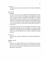
GRINCH User's Manual
Douglas B. Schiff
July 8, 1984
The University of North Carolina at Chapel Hill
Department of Computer Science
New West Hall 035 A
Chapel Hill. N.C. 27514
Table Of Contents
1 Introduction
2 Introduction To GRINCH
2.1 Overview Of The System
2.1.1 Purpose of GRINCH
2.1.2 Features of GRINCH
2.2 Hardware/Software Environment
3 How to Use GRINCH
3.1 Preparing to Use GRINCH
3.2 Tutorial
3.2.1 Command Conventions
3.2.2 Executing GRINCH
3.2.3 Saving and Quitting
3.2 .4 Dynamic Controls
3.2.5 Commands for Viewing
3.2.6 Commands for Interpreting
3.2.7 Building the Model
3.2.8 Miscellaneous Commands
4 Reference Manual
4.1 Notation
4.2 Commands
4.2.1 Viewing
4.2.2 Interpreting
4.2.3 Program Control
4.2.4 Escape Menu commands
4.2.5 Miscellaneous
5 Creating a Ridge-Line Graph
5.1 Data and Information Needed
5.1.1 Density Data
5.1.2 Information About the Data
5.2 Preparing the Data
5 .3 Executing mkskel
5.3.1 The Map File
5.3.2 The Map Information File
Index to Commands
References .
1
2
2
2
3
5
6
6
6
7
7
9
10
11
12
16
19
20
20
21
21
23
28
30
31
32
32
32
32
33
34
34
34
37
38
Chapter 1
Introduction
This manual is is an introduction to, and reference manual for, the GRINCH computer
graphics system for interpreting electron density maps. It is intended for both first time
and experienced users.
Chapter 2 describes the system. It presents an overview of GRINCH's functions and
features and describes the computer environment of the system.
Chapter 3 is a tutorial for the first time user. It provides instructions for the most
commonly used commands and should be worked through sequentially while running the
program.
Chapter 4 is a reference manual. It provides detailed definitions and explanations
of all GRINCH commands. Commands are grouped by function and listed alphabetically
within groups.
Chapter 5 is a tutorial for creating GRINCH ridge-line graphs from electron density
data.
The index provides reference for all commands.
Chapter 2
Introduction To GRINCH
(Graphical Ridge Line Interpretation- Chapel Hill) is a tool to help the
GRINCH
user interpret electron density maps of crystallized proteins. It was originally developed
at the University of North Carolina at Chapel Hill in 1982 by Thomas Williams, as part of
his work towards the Ph.D. in computer science, under the supervision of Dr. Frederick P.
Brooks, Jr. Since then, visiting biochemists and
c~stallographers
have done extensive
work using the system. Their feedback has been used to expand and refine
GRINCH.
Ail it
stands, it is the work of Williams, Tom Hern, Mike Pique, Dare Rosenblum, Doug Schiff,
Brian VanDuzee, and Lee Westover.
2.1 Overview Of The System
2.1..1 Purpose of GRINCH
was designed to supplement or replace the manual mms-map method of
GRINCH
interpreting electron density maps. It provides essentially the same functions but with far
greater power.
The principal function is the identification of the structures of a protein molecule.
The
GRINCH
user is able to locate efficiently and to identify the
main chain, as well as
secondary structures, of a protein molecule. The user can then continue the process to
identify sidechains and carbonyl oxygens.
In addition,
GRINCH
provides functions to build a three-dimensional model of the
protein molecule. Amino acid residues can be selected from a menu and associated with
the sidechains and carbonyls identified in the density data. This model, its residue types,
atom types, and atom coordinates are available as output from the program.
GRINCH
is one component in a larger analytic context.
GRINCH
provides no functions
for modifying the model; bonds cannot be rotated, and angles cannot be adjusted. After
identifying atoms which account for the electron density, the user must rely upon other
systems to fit those atoms to the electron density; e.g.
[Britton, 1977] [Brooks, Jr, 1977] or
FRODO
GRIP-75
[Jones, 1979].
[Tsernoglou et al., 1977]
3
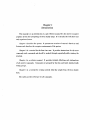
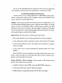
Figure 2.1: Peaks, Passes and Ridge Lines in Terrain.
:Z.l.:Z Features of GRINCH
Representation of the Density Map. The key element of the
GRINCH
system is its
ridge-line representation of electron density maps. Ridge lines connecting local density
maxima are analogous to ridges in a geographic terrain.
In describing terrain, local maxima are called peaks and saddle points are called pasaes.
Ridges are the paths of steepest ascent from passes to peaks (Figure 2.1). That is, they
run from peak to pass to peak. Each point on a ridge is a local maximum with respect to
points in the direction perpendicular to the ridge, Precisely the same concepts describe
ridge lines in electron density.
Ridge lines can be also be thought of as lines running through the centers of the tubes
formed by a contour line representation of electron density. For a detailed discussion of
ridge lines see Williams' dissertation [Williams, 1982].
Representing electron density with ridge lines offers three advantages over contour
line representation:
4
First, ridge lines approximate the stick-figure model of a molecule. Therefore, ridge
lines representing the density of a protein structure often resemble the user's intuitive
notion of the shape of that structure. This similarity aids identification.
Second, far fewer lines are required to represent density with ridge lines than with
contour lines. This is important for two reasons. The number of lines that can be displayed
on a graphics device is limited; the number of lines a user can successfully comprehend
is also limited. Consequently, one may view a larger portion of a map and have a more
global view of a ridge-line representation than of a contour line representation.
Third, because there are relatively few ridge lines, each edge of a ridge line can be
associated with a specific level of density (that of its mid-point), and ridge lines above a
certain density level can be selectively displayed. With
GRINCH,
a user can dynamically
change the level of density above which lines are displayed. This dynamic level-changing
is a powerful aid in interpreting electron density; and is generally available only with
considerable delay for contour line representations.
Display Features.
GRINCH
provides a full array of display functions, controlling both
the objects to be displayed and the user's view of these objects. The user can display the
ridge-line map and/or the constructed model. The user may also select various features
for display, such as edges identified as belonging to the mainchain, or edges that have not
yet been interpreted. The scale and center point of the viewing window can be changed
interactively (short delay). The objects can be rotated along any of three axes dynamically
(no delay) with a joystick or dials.
Interpretation Functions.
GRINCH
uses different colors to identify features of a ridge-
line map. With a picking device (tablet and puck, or mouse), the user may select ridge-line
edges and color them according to type, e.g. green for mainchain, purple for sidechain.
The edges may be colored singly, or
GRINCH
can locate contiguous paths of edges of a
single type to speed interpretation.
GRINCH
also provides functions for building a model of the protein molecule. The
user selects from a menu of amino acids and indicates the part of the interpreted map
that corresponds to that residue. Using a least squares approximation, a model of the
residue is fitted to the designated density and is connected to existing adjacent residues.
An additional feature allows the user to compare a known sequence of amino acids with
a sequence built on the system. The feedback provided by
below.
GRINCH
is discussed in detail
5
The user can also add landmark8 to the original map. These can be any configuration
of line segments to mark locations in the density map, e.g. metal atoms or helices.
:z.:z Hardware/Software Environment
At UNC,
GRINCH
GRINCH
is run on a VAX-11/780 with the 4.2 BSD UNIX operating system.
is written almost entirely in the C language, except for some display functions
that are dependent on specific display devices.
Displays. At this time, the complete GRINCH system operates on two display devices. One
is the Adage-Ikonas RDS-3000 graphics system, a high speed raster display. The display
routines are written in GIA2 [Bishop, 1982], a locally developed compiler for the AMD
2900 based microprocessor in the Ikonas. The other display is the Evans and Sutherland
Color Picture System 300, a color line-drawing display. Routines for this device are written
in the graphics language provided with the display.
Input Devices. The
GRINCH
system at UNC uses four input devices.
• The terminal keyboard is used to begin execution and to give some commands.
• A three-dimensional joystick or viewpointer is used to control rotation of the display.
• A puck and data tablet are used to select items from the menus and to designate
edges in the display.
• A slide control is used to control dynamically the minimum density level of edges
displayed.
When the PS300 is used as the display, its own dedicated input devices may be used
instead. A stylus and tablet are used for picks, three dials are used for rotations, and a
fourth is used as the dynamic level control.
Porting GRINCH : Work in Progress. Present research at UNC includes porting
GRINCH
to three different host environments:
o a graphics workstation running UNIX, such as the MASSCOMP workstation.
• a VAX running VMS using theE & S PS300 as the display.
• an IBM mainframe running MVS using the E & S PS300 as the display.
Chapter 3
How to Use GRINCH
This chapter provides an introduction to GRINCH for the new user. It includes step-bystep instructions for executing the program, for controlling the system, and for producing
output. Unless otherwise noted, the procedures described are applicable for all
GRINCH
sites regardless of the host computer system.
3.1 Preparing to Use GRINCH
To proceed with the tutorial you must complete the following preparations.
The Host System. You must have a basic knowledge \)f the host system. On a system
running UNIX, you must know how to log on, how to access the
GRINCH
program, and
how to access files of data.
The Graphics System. You must know which graphics device you can use for display
and which analog-to-digital input devices (joysticks, dials, etc.) you can use for control.
Preparation of Data.
You must have a ridge-line graph, as briefly described in
Chapter 2, for loading into the
GRINCH
program. Chapter 5 explains how to make a
ridge-line graph from electron density data.
3.2 Tutorial
This tutorial is intended to be worked through sequentially while actually running
GRINCH.
Many GRINCH commands are introduced and explained here; detailed descriptions
of all commands are found in Chapter 4, the reference manual.
Most instructions described below are machine and operating-system independent. A
few commands, such as the start-up procedure, are not. The presumed system context
for this tutorial is the UNIX operating system. Information on different systems should
be gotten from local computer personnel.
7
3.2.1 Command Conventions
• All
GRINCH
commands use prefix syntax; the command is given first followed by any
arguments.
• Commands may be either picked from the menu or entered from the keyboard unless
otherwise noted. Commands entered from the keyboard must be followed by hitting
the return key.
• Throughout the manual commands are printed in boldface.
3.2.2 Executing GRINCH
Running Interp. Begin by logging on to your host computer. The command you give
to execute
GRINCH
at UNC is interp. The command is optionally, but usually, followed
by specifying the graphics display device to be used, preceded by a hyphen (e.g. -ps, -vg,
-ik). For example, if you are using an Evans and Sutherland PS300, type
interp -pa
If the file interp is not in your current working directory, you may have to give its full
pathname. Here at UNC you would type
/unc/grip/rl/intarp -pa
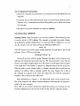
You should now have
GRINCH
running. Messages will appear on the terminal screen
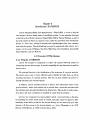
indicating the initialization procedure being run. The main menu and a cursor will next
appear on the graphics display (Figure 3.1). The cursor is a small square when it appears
in the graph area of the display. It changes to a diamond shape in the the menu area.
When you make a pick it changes briefly to a triangle, indicating that the pick has been
registered. In addition, when a command is picked, the cursor changes color to that of
the command as it appears in the menu and retains that color until the command is
completed. This is discussed more fully below.
When initialization is complete, a '#' symbol will appear on the terminal screen.
This is the prompt for the
GRINCH
command interpreter indicating that the program is
ready for the next command.
(Note: Had you not included -pe when you started the program, you could now give the
command displayon pa to get the same result. See the reference manual for details.)
8
mam
side
unkn
m
s
0
b
u
{1
f2
res
add
del
undo
redo
sbow
lev
szze
big
smal
cen
3.8-.------u---
10
t-1-t---
esc
Figure 3.1: Main Menu
Loading a File. You are now ready to load a ridge-line graph. If the name of the file
containing the graph is protein.g (.g for graph), type the command
load protein.g
If the file is not in your current working directory you will need to give its full
pathname. The time it takes to load varies considerably with the size of the file, as
well as other system related factors. A wait of a minute or so is not uncommon. If the
error message 'File Not Found' appears, check the name and/or pathname of the file.
A cube-shaped subset of the map space, called the view cube, will appear on the
graphics display when the file is loaded. The terminal screen will display information
9
about the file and the display. Next to the word width is the length, in Angstroms, of an
edge of the view cube. The coordinates (in map space) of the center of the view cube are
also displayed. Finally, the '#' prompt will reappear.
If the file appears to load but is not displayed, it's possible that the width or level of
the view cube needs to be adjusted.
1. The level number appears on the bottom right of the graphics display to the left of
a horizontal line. Try lowering the level with the dynamic level control (slider or
dial). If this doesn't reduce the level (to near zero) you must change the absolute
level threshold. Try typing 'lovol 0'.
2. The width of the view cube appears on the terminal screen. If it is a small number
(less than twenty), try typing 'window'. This will display the entire map space.
The Graphics Display. Once the map is displayed, the bottom of the graphics display
has some frequently used information. On the left are two white lines: one marked 3.8
and the other 1.5. These indicate the current scale for 3.8A (the length of a C-C bond in
a sidechain) and 1.5A (the distance between C alpha atoms of adjacent residues).
To the right of these lines is a horizontal line scale representing the range of map-edge
density levels. The two vertical bars crossing this scale indicate where the current absolute
and dynamic minimum density level thresholds lie within the range of possible values.
The number to the left of the scale represents the current dynamic minimum density level
threshold (corresponding to the rightmost vertical bar). Only edges with a density level
greater than this value will be displayed. This is discussed in greater detail below.
At the bottom left is a set of coordinate axes. This gnomon indicates the orientation
of the map's coordinate system.
a.z.s Saving and
Quitting
This section explains the procedures for ending a GRINCH session. Of course you've
just begun, but this will enable you to stop at any point in the tutorial and resume at
another time.
Saving. After you have made changes in the map and/or model, you can write the data to
a file with with the save command. We recommend that users number consecutively the
different versions of their files and that they use the '.g' suffix for these GRINCH·Ioadable
files. If the name of the initial file was protein.g, type
eave proteinl.g
10
If the file named already exists, it will be written over; if not, a new file will be created.
This file is in a form suitable for loading by
GRINCH.
It stores complete information about
the map and model as well as the current width, center, and level being displayed. Hence,
reloading the file will restore the same view (aside from rotations) that was being displayed
when it was saved.
Quitting. To end a
GRINCH
session, type the command:
quit
If you have not made any changes in the map or model since the last save command,
the program will terminate. If you have made changes and have not saved them,
GRINCH
will ask for confirmation. The confirmation is entered at the keyboard. Typing yeo will
terminate the program, and any changes made to the file since the last save will be lost.
Typing no will cancel the quit command and return the prompt. At this point, you can
save the file or continue in work. (Note: This command can also be picked from the escape
menu. This is discussed below.)
The same confirmation is required if you try to load a new file when the current file
has been changed and not saved. In this case, typing yea results in the new file being
loaded, and the current file being discarded (along with your changes!).
3.2.4 Dynamic Controls
If you have quit, run interp again and reload your ridge-line map. With the map on
the display, try rotating it using the joystick or dials. You should be able to rotate it about
three different axes. Now move the dynamic level control
~
a slider or dial. It adjusts
the effective minimum density level threshold. As the number increases, fewer edges will
be displayed; edges that remain have density values above the threshold.
Also, try moving the cursor using the puck, mouse, or stylus. It will appear as a small
square when in the display area, as a diamond when near the menu, and as a vertical
bar if you go too far to the right. Notice that it moves smoothly in the area of the map
display, but that it moves discretely (making small jumps) when in the area of the menu.
This discrete jumping avoids ambiguous menu picks.
11
3.2.5 Commands for Viewing
Size Commands. The first series of commands, big, small, and size, change the width
of the view cube. Move the cursor to the command big on the menu and pick (press a
button on the puck or push on the stylus). The cursor should change shape to a triangle,
and then back, indicating the pick was registered. The word bigger should appear on the
terminal screen. The effect of this command is to zoom in on the picture. It actually
decreases the width of the view cube by 20%. Notice that the new width appears on the
terminal screen. Picking the small command zootnll out, increasing the width by 25%.
Therefore, big followed by small, or vice versa, results in no net change.
Now pick the size command. The size menu should appear (Figure 3.2). Picking
a number from this menu will change the width of the view cube to that number of
angstroms.
This is useful for making more extreme changes in tpe scale than those
provided by big and small.
5
0
10
2
15
4
20
6
25
8
30
10
35
12
40
14
45
16
50
18
55
20
60
22
70
24
80
26
90
28
30
full
31
esc
esc
Figure 3.2: Size Menu
Figure 3.3: Level Menu
12
The full command, which appears on the size menu, changes the center and width
of the view cube so that the entire map is displayed as large as possible.
Each of these viewing commands, as well as all commands discussed below, can be
entered from the keyboard as well as picked from a menu. For example, you can type
width 12.0
to change to a view cube with a width of 12A. Note that the number must have a decimal
point. See the reference manual for details on keyboard entry of all commands.
Center Command. You can change the location of the view cube with the center
command. First, pick center on the menu. Next, move the cursor to a map edge and
make a pick (you can only pick edges, not endpoints). The cursor will change to a triangle
when the pick has been registered, then return to a square. The center of the view cube will
now be moved to the midpoint of the edge picked. Alternatively, x, y, and z coordinates
can be entered from the keyboard.
This command is useful for moving laterally through a map while, for example,
identifying the mainchain. It is also used for moving to known locations in the map
space.
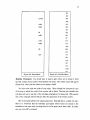
Level Command. When a ridge-line graph is calculated, each edge is assigned a level
number, on an arbitrary scale between 0 and 32, corresponding to its associated electron
density. The level command changes the absolute minimum density level threshold. Pick
level from the menu. A new menu showing numbers from 0 to 32 is displayed (Figure 3.3).
Pick one of the numbers from this menu. Edges with a lower density level will not be
displayed. The dynamic level control can increase this threshold, but cannot decrease it.
This command is useful for getting better response when looking at large sections
of the map since increasing the absolute level threshold reduces the number of edges
involved in calculations. The dynamic level control (slider) affects only the display, not
the calculations.
3.3.6 Commands for Interpreting
Begin this section by changing the width of the view cube to 15A. Experience has
shown this to be a reasonable scale for interpreting map edges. (Make sure there are
enough edges visible for interpreting. H not, change the center to a new location.)
13
In
GRINCH,
colors are IIJ!ed to identify interpreted map edges:
green
for
mainchain
pnrple
for
sidechain
red
for
oxygen
brown
for
disulfide bridges, hydrogen bonds, etc.
white
for
unknown (uninterpreted)
yellow
for
flags or markers
light blue
for
flags or markers
Single Edges. Pick M from the menu. The cursor should turn green. Now pick a white
edge (try to pick one from a chain of connected white edges). The single edge picked
turns green and the cursor remains green. Until a different command is picked you may
continue to color white edges green without picking M again.
Each of the following commands works in the same way, allowing multiple picks and
coloring a single edge at a time:
M
for
mainchain
s
for
sidechain
0
for
oxygen
B
for
disulfide bridges, hydrogen bonds, etc.
u
for
unknown (uninterpreted)
Fl
F2
for
flag 1
for
flag 2
Multiple Edges. To speed interpretation,
GRINCH
provides an alternate method for
identifying longer chains of mainchain, sidechain, and unknown map edges.
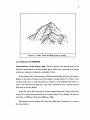
Pick main from the menu: The cursor again turns green. Now pick an unknown
edge that is connected to a chain of white edges which connect to mainchain (Figure 3.4).
GRINCH
will search adjacent chains of white edges and will find the shortest path to existing
mainchain. The edge picked, and all edges in that shortest path, are made mainchain edges
and colored green.
14
Figure 3.4
Alternatively, if an edge is picked between two sections of mainchain (Figure 3.5), the
shortest path of unknown edges to each will be found and colored. This, in effect, makes
one longer chain of the two original chains.
Figure 3.5
There are certain patterns
GRINCH
knows to disallow, such as loops or forks in the
mainchain, and an error will be displayed should these be found. If no path is found,
the single edge selected is made mainchain. Note, also, that this command allows only a
single pick, and the cursor reverts to white.
The side command has a similar function and is generally used for coloring small
subgraphs of white edges attached to mainchain at a single point (Figure 3.6). An edge
of this subgraph may be picked to make the entire subgraph type tidechain.
15
Figure 3.6
If the subgraph selected is attached to mainchain at two points, an error is returned.
One of the purposes of the B (bridge) command is to get around this limitation. Identify
as type bridge all but one of the edges connected to mainchain. This will enable the side
command to color the rest of the subgraph.
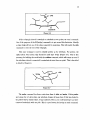
This same technique is used to identify prolene as the sidethain. For prolene, the
alpha-carbon beta-carbon edge should be made type bridge (Figure 3. 7). This is also
necessary for building the model with the residue command, which will return an error if
the sidechain selected is connected to mainchain at more than one point. This is described
in detail in Chapter 4.
aldo
bridge
Figure 3.7
The unkn command has fewer restrictions than do side and main. Picking unkn
and a map edge of a given type, say sidechain, changes all map edges of that type linked to
the picked edge by similar edges, to type unknown. Hence, you could uninterpret an entire
connected mainchain with one pick. This is a good reason for having an undo command.
16
Undo, Redo, and History. Most
GRINCH
commands are undoab/e and the system
enables the user to back up through a sequence of commands. Type h at the keyboard.
This history command returns a list of up to your last twenty undoable commands.
Now pick undo from the menu. It should undo the last undoable command you gave.
Pick undo again. It should undo the previous undoab/e command.
Now pick redo. It should redo the last command undone. Pick redo again. It will
redo your previous undo. Pick redo one more time. You should get an error. Redo only
redoes consecutive undo commands.
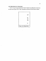
Selective Display of Edges. At this point, you should have some interpreted (colored)
edges on the display.. If not, color some edges before executing the next command. Pick
show from the menu. The show menu will be displayed (Figure 3.8). Now pick any
combination of the edge classifications listed in the menu, completing the command by
picking end. After the command is executed, only edges fitting into one or more of the
categories chosen will be displayed. This remains in effect until the show command is
·executed again.
Try displaying just maincbain edges with the sequence of picks
show main end
(Note that at this time there are no model or fit edges. These will appear in the next
section.) Detailed explanations of the choices are given in the reference manual.
3.2.'1 Building the Model
To do this section of the tutorial, you'll need some interpreted edges. If you haven't
already done so, color some possible stretches of mainchain, as well as some sidechains
and oxygens (Figure 3.10). These identifications need only be conceivable, not convincing.
(In fact, you'll be able to build a model from mainchain alone if sidechain and/or oxygen
edges are missing from the map.)
aideehaln
oxygen
Figure 3.10
17
ala
arg
model
asn
asp
mam
cys
allmc
gln
glu
fit
gly
unfit
his
ile
color
leu
unkn
lys
met
phe
all
pro
ser
end
thr
trp
tyr
val
none
esc
Figure 3.8: Show Menu
Figure 3.9: Residue Menu
Residue Command. You should have in mind a place where you're going to build
the first residue of your model. Pick res from the menu. The residue menu will appear
(Figure 3.9). Next, pick the residue you're going to build.
You must now make two picks of map edges. These identify the interpreted edges
of the map to which the model of the residue will be fitted. The first pick identifies the
sidechain and can be any edge of the sidechain subgraph you've interpreted. (The specific
edge of the sub graph selected will not affect the placement of the residue model.)
The second pick indicates the oxygen placement. Typically this is a single red edge.
There is a restriction that the sidechain and oxygen selected must not attach to the
mainchain at the same node, nor may they be too far apart (more than 3.8A ). In either
case, an error will be returned.
18
A few seconds after the last pick, the main menu should reappear. Following this,
a blue model of the residue selected will appear in the identified location. If you are
dissatisfied with the selection or placement, there are two ways to undo it. You can use
the undo command, or you can replace the residue you built with residue none. To do
the latter, you must follow the same sequence of steps as above (e.g. pick res, pick none,
and pick two map edges. They need not be the same two edges picked when building the
residue, but they must be. associated with the residue.)
Missing Sidecbain or Oxygen. It is not uncommon for there to be no sidechain and/or
oxygen edges along part of a mainchain of a ridge-line map.
GRINCH
will build a residue
with either or both missing if appropriate picks of mainchain map edges are used to
indicate where the sidechain and oxygen should connect to the mainchain.
Try this on any sequence of mainchain map edges where no residue has been fitted.
(There must be at least three consecutive green edges.) Pick res followed by a residue
type. Then, to identify the sidechain location, pick a mainchain map edge. The sidechain
will be built at the endpoint of the selected edge closest to the oxygen you will select
(Figure 3.11). Similarly, pick a mainchain map edge for the oxygen. The oxygen will be
attached at the endpoint of the selected edge closest to the sidechain chosen. Note that
the two picked edges must not be adjacent, nor may they be too far apart (more than
a.s.A.).
sldechaln
attaehed here
piek for
oldechaln
oxygen
attaehed here
t
piek for
oxyg~n
Figure 3.11
Try building some adjacent residue models. Notice that
GRINCH
connects one to the
other. You might also try the show command with the fit, unfit, and model choices, now
that some residues have been fitted.
19
3.2.8 Miscellaneous Commands
There is one more menu of commands which is displayed by picking esc (escape) from
the main menu (Figure 3.12). These commands are discussed in the reference manual.
quit
seq
info
dist
esc
Figure 3.12: Escape Menu
Chapter 4
Reference Manual
4.1 Notation
The following notation is used in this chapter:
• Commands are printed in boldface.
• Commands may be either picked from the menu or entered from the keyboard unless
otherwise noted.
• Alternate spellings for a command are listed in parentheses. Any of these may be
keyed in, though only one will be found on the menus.
• Arguments are printed in italics and may be one of the following types:
o integer - a number without a decimal point picked from a menu or entered from
the keyboard
o Boat - a number with a decimal point picked from a menu or entered from the
keyboard
o edge or map.edge - an edge picked from the display or keyed as 'a' followed by
the edge number, ie. e1234
o residuetype - one of twenty amino acids, picked from the menu or typed using the
corresponding number ( 1 to 20; 0 for none).
o filename - any acceptable system filename entered from the keyboard
o resnum - any residue from the model; selected from the display by picking any
associated edge, or keyed as 'r' followed by the residue number, ie. r90
• Arguments in brackets ( [ ] ) indicate a choice of those listed.
21
• Ar~>Uments followed by a plllil ( +) indicate that one or more may be selected.
The commands are divided into four categories: viewing, interpreting, program
control, and miscellaneoUl!. Within each category, the listing is alphabetical. The index
provides an alphabetical listing of all the commands.
4.2 Commands
4.2.1 Viewmg
The volume of the map space that is visible is always a cube and is referred to as the
view cube. The width of the view cube is the length of an edge of the cube, in angstroms.
That is, a width of 10.0 means that 10.0 x 10.0 x 10.0 cubic angstroms of map space are
visible. The width and center point of the view cube appear on the terminal screen after
any change.
bigger
( big )
The edges displayed are made bigger (zoom in) by decreasing the width of the view
cube by 20%. The new width , in angstroms, appears on the terminal screen.
center edge
( een )
The center of the view cube is set to the midpoint of the selected edge. Use this to
move to different parts of the map space. The coordinates of the new center point are
displayed on the terminal screen.
center float float float
( een )
The three numbers represent the x, y, and z coordinates, in angstroms, of a point in
the map space. The center of the view cube is set to this point. The coordinates of
the new center point are displayed on the terminal screen.
level integer
( lev )
The minimum absolute density level threshold is set to the specified number.
Each edge in a ridge-line map has an associated electron density value between 0 and
32. This value is determined by mk•kel, the program that calculates the ridge-line
22
graph from the electron density data. Mkskel scales the original range of densities to
this smaller range.
Only map edges with a density value higher than the absolute threshold are included
in the calculation of the display. The dynamic level control (slider or dial) affects
only those edges included in this calculation. Hence, the slider can make the effective
threshold greater than, but not less than, the absolute threshold. The current absolute
and dynamic thresholds are displayed at the bottom right of the graphics screen.
(Note: This command exists only for performance reasons. For example, changes in
the view cube will occur more rapidly with a higher absolute threshold because a
smaller number of map edges will be included in the calculation of the display.)
show [ all model main allmc fit unfit unknown]+ end
Only edges fitting into one or more of the specified categories (within the current view
cube) are displayed. This remains in effect until the next show command or until a
new file is loaded. The arguments are defined as follows:
all
all map and model edges
model
all model (blue) edges
masn
mainchain map edges
allme
mainchain map and model edges
fit
map edges to which a residue model has been fit; this includes
mainchain, sidechain, and oxygen edges associated with a specific
unfit
residue
map edges to which no residue model has been fit
unknown
map edges which have not been interpreted (white edges)
color
map edges which have been interpreted (green, purple, red, and
brown edges)
Any combination of arguments can be selected, and the results are additive. The list
of arguments must be followed by the command, end (endshow, if entered from the
keyboard).
size float
( width )
Displays the size menu, from which a number can be selected. The width of the view
cube is set to the chosen number of angstroms. This command is useful for changes
in scale greater than the changes produced by big and small. The new width is
displayed on the terminal screen.
23
size full
(width)
The width and center of the view cube are set so that the entire map and model are
in the view cube and are displayed as large as possible. The new center and width are
displayed on the terminal screen. (Note: This command is only available as a menu
pick. See window for the corresponding keyboard command.)
smaller
( omal, oman )
The edges displayed are made smaller (zoom out) by increasing the width of the view
cube by 25%. The new width , in angstroms, appears on the terminal screen.
window
The width and center of the view cube are set so that the entire map and model are
in the view cube and are displayed as large as possible. The new center and width
are displayed on the terminal screen. (Note: This command is only available as a
keyboard command. See size full for the corresponding menu pick.)
4.:1.:1 Interpreting
bridge
map~edge
+
( B, b, br)
The selected edges are identified as type bridge and colored brown. Multiple picks are
possible.
This command is intended for identifying such structures as disulfide bridges and
hydrogen bonds. In addition,
GRINCH
will not allow certain configurations of edges,
such as a sidechain touching a mainchain in more than one point (in a prolene ring, for
example). In this situation, all but one of the sidechain edges connected to mainchain
should be made type bridge.
ftagl
map~edge
+
( Fl, n )
The selected edges are colored light blue. Multiple picks are possible. This command
is intended for identifying edges of the map as markers. For example, edges added by
the user might be marked for later scrutiny, or edges along the boundary of a molecule
could be identified. This is useful for orientation in global views of the map.
24
flag2 map_edge
+
( F2, 1'2 )
The selected edges are colored yellow (See flagl).
main map_edge
( me, malnehaln )
Searches for the shortest path of visible, unknown (white) edges from the edge selected
to a visible mainchain edge. If a path is found, all the edges in the path are identified as
type mainchain and colored green. If not, only the selected edge becomes mainchain.
Interpreting mainchain with this command proceeds much more rapidly than by
selecting a single edge at a time.
It can be used in two ways. A single existing
chain of mainchain edges can be extended, or an edge between two separate chains
of mainchain edges can be selected and the path between the two will be found and
interpreted. Note that the command will not create branches or loops in the chain.
M map_edge
+
The selected edges are made type mainchain and are colored green. Multiple picks
are possible.
residue residue_type map_edgel map_edge2
( reo )
A model of the selected residue is built and fitted to the part of the map indicated
by the edges selected. In the most common case there is a subgraph of sidechain
map edges connected to the mainchain at one node, and an oxygen edge connected
at a different node. Map_edgel indicates the sidechain and can be any edge in the
subgraph of sidechain edges. Map_edge2 indicates the oxygen edge.
If there are no sidechain edges, a mainchain map edge may be chosen for map_edgel.
In this case, the sidechain is inferred to be attached to the endpoint of map_edge 1
closest to map_edge2.
If no oxygen edge exists, a mainchain edge may be chosen for map_edge2. The oxygen
is inferred to be attached to the endpoint of map_edge2 closest to map_edge 1.
If neither sidechain nor oxygen edges exist, the two mainchain edges selected must
have at least one edge between them, and may be no farther than 3.8A apart.
25
sequence res1 res2
( seq )
Matches a sequence of residues which have been fitted to the map, to the known
residue sequence. The two residue arguments, resl and res2, must be connected by
a sequence of residues. Either resl or res2 may be the amino end of the specified
sequence.
G
4
1
2
4
4
I
A
10
1
3
5
5
I
s
8
1
8
3
3
I
T
2
1
10
1
1
I
v
2
1
8
1
1
I
p
3
1
5
1
1
I
1
1
1
5
1
1
I
L
1
4
2
2
2
I
N
1
3
3
2
2
I
D
2
3
3
2
2
Q 1
E 2
G 3
3
3
2
2
I
3
3
2
2
I
1
7
1
1
I
M
1
5
2
4
4
I
K
2
2
2
10
10 I
R
1
2
1
7
7
I
H
1
8
1
2
2
I
v
1
10
1
2
2
I
y
1
8
1
2
2
I
w
1
6
1
1
1
I
,
I
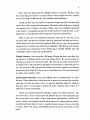
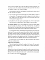
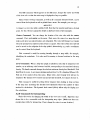
Figure 4.1: Sequence Command Trial Matrix
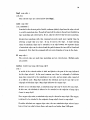
The computer initially constructs a trial matrix, T, with one column for every residue
in the chain specified by res1 and rea!!, and one row for each residue type (Figure 4.1).
An element of the jlh row and /h column of T gives an estimate of the probability
that the jth residue fitted really is of the type in row i. The probability ratings are
26
based upon structural comparisons between the fitted residue and each residue type.
Values range from a worst rating of 1 to a best rating of 10.
Matrix Tis presented through the vi text editor [Joy, 1980] so that the user may alter
the matrix for the specific environment of the residues that were fitted. Matrix entries
can be changed, using commands in vi, to increase or decrease the probability values
for specific residues, or the initial values may be used. When the matrix contains the
desired values, exit the editor with the command :wq or the command ZZ.
The resulting matrix is used to match the specified sequence to the known sequence.
The known sequence must be in a file named sequence when program execution begins.
Three-letter or one-letter abbreviations may be used, with entries separated by blanks
or newlines; all letters must be upper case.
43 s H
36 A F
33 T H
30 A
A
T
R
K I 7
T
I
A
I 1
s
K
A
I 9R
M
K
R I 14R
28 A I T
25 A M K
23 A K s
F A I 5R
R ~ I 13R
H T I 5
22 F
T
I
A
K I 2
19
I
A
K
R
T
A
s
s
T
19 K
I 3
I 11R
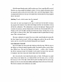
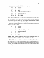
Figure 4.2: Top Ten Rated Registrations
GRINCH
tries each possible registration of the specified sequence with the known
sequence, in both directions. A sum of the appropriate matrix elements is computed
and the user is presented with the top ten rated registrations (Figure 4.2). The number
on the left of each row is the •core of the registration. The number on the right is
the position, within the known sequence, of the registration. An R indicates that the
sequence is reversed.
In the present implementation, no further action is taken by the computer; the user
must make any changes required to match his/her fitted sequence with the registration
chosen.
27
S map_edge
+
The selected edges are made type sidechain and are colored purple. Multiple picks
are possible.
side map_edge
( sc, sldeehain )
Searches for the largest connected sub graph of visible, unknown( white) map edges
connected to the selected edge. If the subgraph touches mainchain in exactly one
point, all the edges are made type sidechain and colored purple. If the subgraph
touches mainchain in more than one point, no action is taken and an error message is
displayed on the terminal screen. If the subgraph does not touch mainchain at all, it
is cut into two parts at the selected edge, and only the selected edge and the smaller
part are made type sidechain. No action is taken if a path of length greater than 14
A
exists in the set.
If the sub graph is supposed to connect to the mainchain in two points (e.g. prolene ),
the alpha-carbon beta-carbon edge must be identified as some other type (usually
bridge) before the side command can be used. Furthermore, the residue command
will return an error if the sidechain selected is attached to mainchain at two points
(see above).
U map_edge
+
The selected edges are made type unknown and are colored white. Multiple picks are
possible.
unknown map_edge
( unkn )
All edges in the subgraph containing the selected edge (edges of the same type,
connected to it by edges of the same type) are made type unknown and colored
white. (Note the lack of restrictions! This command can color an entire connected
mainchain white with one pick.)
28
4.2.3 Program Control
displayon name
Turns on the display named. Recognized names are:
ik, ikonas
Adage-lkonas RDS3000
ps, ps300
Evans Sutherland PS300
vg
Vector General
nvg
Vector General 3033
crt
Terminal Screen
This command can only be entered from the keyboard.
displayolf name
Turns off the display named. See displayon.
escape
( eae )
When selected from the main menu, this command displays the escape menu which
includes the commands quit, seq, info, and dist. When selected from any other
menu, the main menu is displayed and the '#'prompt returns.
h
The history command displays the last twenty 'undoable' commands (see undo). This
command can only be entered from the keyboard.
inputon name
Turns on the input device named. Recognized names are:
tablet
puck and data tablet
viewpointer, vuptr, joystick
3-d viewpointer
slider
slider for dynamic level control
keyboard
terminal keyboard
mouse
not implemented
psknobs
PS300 control dials
pstablet
PS300 stylus and data tablet
This command can only be entered from the keyboard. At UNC, the input devices
turned on by default are the 3-d viewpointer, data tablet, and slider.
29
inputolf name
Turns off the input device named. See inputon.
load ( yes no ]
The ridge-line graph file named (in
GRINCH
format, see Chapter V) is loaded into
the program and displayed. It is loaded in the exact form in which it was saved (or
created, if never loaded previously).
If a file is resident in
GRINCH
and has been changed since the last save command,
confirmation of yea or no must be given. A yea indicates that the file will be read and
the resident file discarded. A no aborts the load and returns the prompt for a new
command. At this point, the resident file could be saved and the load tried again.
menuolf
Deletes the menu from the display (useful for photographs). This command can be
entered only from the keyboard.
menu on
Restores the menu to the display; used only after the menuolf command. This
command can only be entered from the keyboard.
redo
Reverses the effects of an immediately preceding undo, with results as if the undo
had never been given. If another redo command is given, it reverses the undo
immediately preceeding the previous undo.
An error is returned if there is no
immediately preceeding undo.
save lllename
The current map, model, and display data are stored in the named file. If the file
already exists, it is overwritten; if not, a new file is created.
30
undo
Reverses the effect of the last command, with results as if that command had never
been given. If another undo is given, it reverses the effect of the command given
prior to the one already undone. In this manner, the user can backup up as many
as twenty commands. An error message is displayed on the terminal screen if there
are no more commands to undo or if the previous command cannot be undone. The
commands, load and save, cannot be undone.
4.Z.4 Escape Menu commands
These commands are displayed when the command, esc, is picked from the main
menu. Each command can also be entered from the keyboard.
add map_edgel map_edge2
An edge of type unknown(white) is added between one endpoint of the first edge
picked and one endpoint of the second edge picked. The endpoints are chosen to make
the new edge as short as possible.
delete map_edge
(del )
The map edge selected is deleted from the display and from the graph.
distance edgel edge2
( dist )
The shortest distance between the endpoints of the first edge and the endpoints of
the second edge is displayed on the terminal screen.
Info edge
All known information about the edge and its endpoints is displayed on the terminal
screen. This includes edgetype, edge number, length, coordinates of the endpoints, fit
or unfit; if fit, then also displayed are the residue type, residue number, atom types
of the endpoints, and whether twistable or not twist able.
31
quit [ yes no ]
To terminate
GRINCH,
type the command, quit. If a file is resident in GRINCH and has
been changed since the last save command, the program will prompt for confirmation
of ye6 or no. Typing ye• indicates that the session will end and that the resident
file will be discarded. Typing no aborts the quit and returns the prompt for a new
command.
4.2.5 Miscellaneous
plot filename
Saves the displayed image in plot format. This is suitable for making hardcopy plots
of the image.
print
Displays, on the terminal screen, detailed information of all nodes and edges in the
current display. This includes node number, node density, edge number, edge type, edge
density, residue type, node number for each endpoint and length of the edge.
This is the same shell escape found in the vi editor. Any acceptable shell command
will be executed, after which the prompt will return and
command.
GRINCH
will await the next
Chapter 5
Creating a Ridge-Line Graph
This chapter describes how to generate a ridge-line graph from an electron density
map using the program mi<Bkel. Graphs generated by mkskel are in the proper format
for loading into
GRINCH.
The process for generating the map is described as it is done at
UNC.
Throughout this chapter, commands (executable files) appear in boldface. Arguments appear in italics. Arguments that appear within brackets ( [ ] ) are optional.
5.1 Data and Information Needed
5.1.1 Density Data
The input to mkskel is a file containing the electron density value at each vertex of a
three-dimensional grid. This data must be from an orthogonal map; mksel cannot work
with triclinic or other non-orthogonal maps.
The values should be stored as ASCII (text) characters, separated by blank spaces.
The file should contain no extraneous marks (e.g. end-of-plane markers). The first line of
such a file might look like:
20.1 12.8 -3.2 18.4 3.2 53.4 30.2 85.3 43.2 -12.0
By convention, the name of the file should end with .a•cii; for example, abcmap.ascii.
5.1.3 Information About the Data
To run mkskel requires the following information:
(1) The sort order of the density values. Since the coordinates of each value are not
included in the file, mkskel must know which dimension of the grid (X, Y, or Z) varies
most quickly, which next most quickly, and which most slowly.
For example, listing the values from the first XY-plane, then the next, and so on,
means that Z varies most slowly. Within each XY-plane, listing all the values for a
given Y coordinate (along the X-dimension) means that Y varies more quickly than
Z, and X varies most quickly.
33
(2) The extent of the map. This is the number of points along each axis of the map. (One
more than the number of spaces!)
(3) The spacing between planes along each axis (in angstroms).
(4) The coordinates of the origin of the map.
(5) The resolution of the map.
(6) The range of values most likely to be usable. To produce the ridge-lines, the programs
described below scale down the range of values considerably. Therefore you must
know not only the actual range of values, {Are there negative values? What are
the approximate maximum and minimum values?) but also the range over which
producing ridge-lines is likely to be fruitful.
5.2 Preparing the Data
The data in the .ascii file described above must be scaled to a prescribed range and
converted to the proper 8-bit (one byte) binary integer format. This process is simplest
when done in 3 steps:
• conversion from ASCII characters to 16-bit binary
• linear scaling up or down in the 16-bit binary form
• conversion from 16-bit binary to 8-bit binary.
This is done with the following three programs.
(1) atomapl6 [ -s scalefactor Jlllenamei [ lllename2]
This program converts ascii numbers (Boating point numbers or integers) to 16-bit
signed integers. The input is taken from filename1. The output is written to standard
out or to the optional fi/ename!J argument. The program also prints the total numbers
processed and the maximum and minimum values of the output (needed for the next
program). If the optional scaling argument is given, each input value is multiplied
by this argument before writing the value out. This option is typically used when
the input map contains Boating point numbers and truncating the values to integers
would lose too much information. For example,
atomapl6 -s 10 abcmap.ascii abcmap.16
would multiply each number in abcmap.ascii by 10 then write it out in 16-bit binary
form to the file abcmap.16.
34
(2) map16map
lowin bighin lowout bighout
This program maps a file of 16-bit signed integers linearly onto a given range. The
/owin and highin values are from the atomap16 output. The lowout and highout values
should be -128 and 127, respectively, for mkskel. The output from atomapl6 may be
redirected into:
map16map -200 500 -128 127
(3) mapl6tobb filein fileout
This program maps 16-bit integers into 8-bit integers.
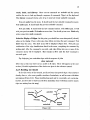
These three programs can be connected in a pipeline:
atomap16 xyzmap.ascii I mapl6map 0 500 0 120 I map16tobb > xyzmap.m
5.3 Exeeuting m.bkel
The mkskel program requires two input files whose filenames must have the same root.
5.3.1 Tbe Map Pile
The first is the file of one-byte binary numbers generated from the density data. This
must be given a filename of the form root. m (m for map) where root is generally some
abbreviation of the molecule name.
5.3.3 Tbe Map Information File
The second, the map information file, contains information about the density data as
well as two variable parameters for adjusting the ridge-line graph produced by mkskel.
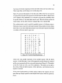
The file must have the format illustrated by the example (Figure 5.1). The name of this
file must be root.mi (mi for map information) where the root is the same as that of the .m
file.
35
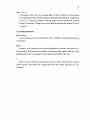
Format
Example
title (usually name of molecule and user)
Deoxypreposterase ABC
sorting order
XZY
extent of map
60 50 72
sample spacing (angstroms)
1.1 0.9 0.8
ongm
-2 0 3
lowest density to be considered for ridge lines 30
largest edge allowed (angstroms)
2.8
Figure 5.1: Map Information File
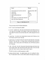
The seven items provide the following information:
l. title - for your use and ignored by mkskel.
2. sort order- explained above. The axis on the left varies the most slowly and the one
on the right, the most quickly. In the example, X v.aries the most slowly and Y the
most quickly. The values in the next three items of the .mi file correspond to the sort
order.
3. extent-of-map - the values in the example show 60 points in the X direction, 50 in
the Z direction, and 72 in the Y direction.
.
'
4. sample spacing- the distance between two consecutive points along the corresponding
dimension. The values show a l.l.A space between consecutive points along the X
dimension, a 0.9.A. between points in the Z dimension, and a 0.8.A between points in
the Y dimension.
5. origin- which plane, row, and column passes through the origin point (0,0,0) of the
map coordinate system. The values show the plane with X value -2, the row in that
plane with Z value 0, and the column in that row with Y value 3.
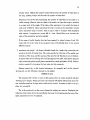
The final two entries are variable parameters to mkskel.
6. minimum ridge-line density - the smallest density value to be considered for ridgelines. The appropriate value here varies with the quality of the map and the range of
36
density values. Making the number smaller will increase the number of ridge-lines in
the map; making it larger will decrease the number of ridge-lines.
Experience has shown that maximizing the number of ridge-lines in the graph is a
useful strategy. However, there is a limit to the number of edges that may be attached
to a single node of the graph. If the value of the parameter is too small, the limit of
each node is filled by edges connecting the node to points in its immediate vicinity
and a degenerate map is created. Such a map is easy to recognize when displayed
with
GRINCH;
it appears as a screen full of ;·-oints. Should this occur, increase the
value of this parameter and rerun mkskel.
If the range of useful density data has been mapped to values between 0 and 120,
begin with 10 as the value of the parameter (you will probably have to try several
different values).
7. maximum edge
length~
the largest allowable length for a single edge connecting two
points in the grid of density data. The value specified is a function of the quality and
resolution of the map, and the spacing of the grid, but the function is not yet defined.
A typical value for a 3.0A map with l.OA spacing has been 2.8A. This allows diagonal
edges connecting points in grid planes separated by a single grid plane ( 2.0A). Further
study is required to determine the best value for this parameter.
Having created the .m file (named abcmap.m, for example) and .mi file (named
abcmap.mi), use the following command to run mkskel:
mkskel abcmap
The program will read the .m and .mi files and produce an output graph file labelled
abcmap.g (g for graph). During execution, the terminal will display information about the
run, including numbers of edges which could not be created. As many as eight to ten per
plane are reasonable.
The .g file produced is in the correct format for loading into
GRINCH.
Displaying the
ridge-line graph using GRINCH is generally the best way of determining whether any of the
input parameters need to be adjusted.
Index to Commands
add, 30
bigger (big), 11, 21
bridge (B, b, br), 13, 15, 23
B, 13, 15, 23
cantor (can, 12, 21
delate (dol), 30
diaplayon, 7~8, 28
diaplo.yoff, 28
distance (diat), 30
escape (eoc), 19, 28, 30
full, 12, 23
F1 (flag1, fi), 13, 23
F2 (flag:!, f2), 13, 24
history (h), 16, 28
info, 30
inputon, 28
inputaff, 29
intarp, 7
level (lov), 9, 12, 21~22
load, 8~9, 29
main (mainchain, me), 13~14, 24
monuoff, 29
manuon, 29
M, 13, 24
o, 13
plot, 31
print, 31
quit, 10, 31
redo, 16, 29
reaidue (rea), 17~18, 24
save, 9--10, 29
aequenca (aaq), 25~26
ohow, 16, 22
aide (oiciechain, oc), 14~15, 27
oize, 11~12, 22~23
smaller (small, omal), 11, 23
s, 13, 27
undo, 16, 30
unknown ( unkn), 15, 27
u, 13, 27
width, 12
window, 9, 23
I (shell escape), 31
References
Bishop, G. 1982. Gary's lkonas Assembler, Version 2; Differences Between Gia2 and C,
TR82-010 UNC Department of Computer Science, Chapel Hill, NC.
Britton, E. G. 1977. A Methodology for the Ergonomic Design of Interactive Computer
Graphic Systems, and its Application to Crystallography, PhD Thesis, University of
North Carolina, Chapel Hill.
Brooks, Jr, F. P. 1977. "The Computer 'Scientist' as Toolsmith: Studies in interactive
Computer Graphics," Proceedings of IFIP.
Jones, T. A. 1979. "A Graphics Model Building and Refinement System for Macromolecules," Journal of Applied Crystallography.
Joy, W. Nov 1980. "An introduction to Display Editing with VI, revised by M. Horton," UNIX Programmer's Manual Volume 2c · Supplementary Documents, Seventh
Edition, Virtual Vax-11 Version.
Tsernoglou, D., G. A. Petsko, J. E. McQueen, and J. Hermans. 1977. "Molecular Graphics:
Application to the Structure Determination of a Snake Venom Neurotoxin," Science,
Vol. 197, 1378-1381.
Williams, T. 1982. A Man-Machine Interface for Interpreting Electron Density Functions,
PhD Thesis, University of North Carolina, Chapel Hill.