Download Trailing edge curve

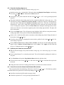
Geometry Modeling and Mesh Generation Strategies for Complex ThreeDimensional Iced Wing Configurations: Year 1 Report (NAG3-2562)
David Thompson, Satish Chalasani, Sanka Gopalsamy, and Bharat Soni
Center for Computational Systems
Mississippi State University
Mississippi State, Mississippi
February 2002
Abstract
The problem of flow field simulation for iced wing configurations is a complex one that severely taxes
existing capabilities for geometry modeling, mesh generation, and flow solvers. In this report, we focus on
activities associated with the first year of a three-year program to develop a software package to facilitate the
numerical simulation of viscous flows around iced wing configurations. We investigated various geometry
modeling and mesh generation technologies to evaluate their effectiveness for application to the iced wing
problem. Based on these evaluations, we developed a basic strategy for attacking the problem. Further, we
were able to demonstrate the complete process—from geometry to mesh to flow solution—for a complex
iced wing configuration.
ii
Contents
1. Introduction
1
2. Problem Description
2
3. Geometry Modeling
3.1 Surface Modeling . . . . . . . . . . . . . . . . . . . . . . . . . .
3.1.1 Fully Three-Dimensional Surface Modeling . . . . . . . .
3.1.2 Pseudo Three-Dimensional Surface Modeling . . . . . . .
3.2 Automatic Surface Extraction . . . . . . . . . . . . . . . . . . . .
3.2.1 Introduction to Level Sets . . . . . . . . . . . . . . . . .
3.2.2 Curve (Surface) Extraction Data using Level Set Methods
4. Mesh Generation
4.1 Issues . . . . . . . . . . . . . . . . . . . . . . . . . . . .
4.2 Procedure . . . . . . . . . . . . . . . . . . . . . . . . . .
4.3 Example Mesh . . . . . . . . . . . . . . . . . . . . . . .
4.4 The ICEWING System . . . . . . . . . . . . . . . . . . .
4.4.1 Rationale . . . . . . . . . . . . . . . . . . . . . .
4.4.2 Topologically-Adaptive Surface Mesh Generation .
4.4.3 Topologically-Adaptive Volume Mesh Generation .
4.4.4 Example Mesh . . . . . . . . . . . . . . . . . . .
.
.
.
.
.
.
.
.
.
.
.
.
.
.
.
.
.
.
.
.
.
.
.
.
.
.
.
.
.
.
.
.
.
.
.
.
.
.
.
.
.
.
.
.
.
.
.
.
.
.
.
.
.
.
.
.
.
.
.
.
.
.
.
.
.
.
.
.
.
.
.
.
.
.
.
.
.
.
.
.
.
.
.
.
.
.
.
.
.
.
.
.
.
.
.
.
.
.
.
.
.
.
.
.
.
.
.
.
.
.
.
.
.
.
.
.
.
.
.
.
.
.
.
.
.
.
.
.
.
.
.
.
.
.
.
.
.
.
.
.
.
.
.
.
.
.
.
.
.
.
.
.
.
.
.
.
.
.
.
.
.
.
.
.
.
.
.
.
.
.
.
.
.
.
.
.
.
.
.
.
.
.
.
.
.
.
.
.
.
.
.
.
.
.
.
.
.
.
.
.
.
.
.
.
.
.
.
.
.
.
.
.
.
.
.
.
.
.
.
.
2
2
4
4
5
5
7
.
.
.
.
.
.
.
.
8
9
9
9
10
10
12
12
14
5. Flow Solution
15
6. Assessment of Existing Capabilities
15
7. Recommendations
17
8. Summary
18
A. Truly Three-Dimensional Surface Modeling
A.1 Create the trailing edge curve . . . . . . . . . . . . . .
A.2 Create the leading edge curve . . . . . . . . . . . . . .
A.3 Split the point cloud into two surfaces . . . . . . . . .
A.4 Create Curves at the Inboard and Outboard Boundaries
A.5 Creation of Surfaces . . . . . . . . . . . . . . . . . .
iii
.
.
.
.
.
.
.
.
.
.
.
.
.
.
.
.
.
.
.
.
.
.
.
.
.
.
.
.
.
.
.
.
.
.
.
.
.
.
.
.
.
.
.
.
.
.
.
.
.
.
.
.
.
.
.
.
.
.
.
.
.
.
.
.
.
.
.
.
.
.
.
.
.
.
.
.
.
.
.
.
.
.
.
.
.
.
.
.
.
.
.
.
.
.
.
.
.
.
.
.
23
23
25
25
25
27
List of Figures
1
2
3
4
5
6
7
8
9
10
11
12
13
14
15
Noisy point cloud data . . . . . . . . . . . . . . . . . . . . . . . . . . . . . .
Fully three-dimensional surface representation . . . . . . . . . . . . . . . .
Pseudo three-dimensional surface representation . . . . . . . . . . . . . . .
Airfoil surface extraction using level sets . . . . . . . . . . . . . . . . . . .
Triangular surface mesh (wing lower surface) . . . . . . . . . . . . . . . . .
Left-side boundary of mesh . . . . . . . . . . . . . . . . . . . . . . . . . . .
Mesh on side boundaries near airfoil . . . . . . . . . . . . . . . . . . . . . .
Cutting planes through the mesh at three spanwise stations (lower surface)
Mesh flaw in left-side boundary plane . . . . . . . . . . . . . . . . . . . . .
Example of simple topological adaptivity in a surface mesh . . . . . . . . .
Topological adaptivity for mesh quality improvement . . . . . . . . . . . .
Near-body volume mesh without topological adaptivity . . . . . . . . . . .
Near-body volume mesh with topological adaptivity . . . . . . . . . . . . .
Navier-Stokes solution for iced wing using Cobalt M=0.3, Re=2.0x10 , Basic Strategy: Generate six curves to define two surfaces . . . . . . . . . .
iv
.
.
.
.
.
.
.
.
.
.
.
.
.
.
.
.
.
.
.
.
.
.
.
.
.
.
.
.
.
.
.
.
.
.
.
.
.
.
.
.
.
.
.
.
.
.
.
.
.
.
.
.
.
.
.
.
.
.
.
.
.
.
.
.
.
.
. . . . .
.
.
.
.
.
.
.
.
.
.
.
.
.
.
.
.
.
.
.
.
.
.
.
.
.
.
.
.
.
.
3
5
6
8
10
11
12
13
14
15
16
17
18
19
24
1. Introduction
There are two distinct applications related to the aircraft icing problem in which computational fluid dynamics (CFD) can play a significant role [1]. First is the prediction of ice accretion using a code such as
LEWICE [2] coupled with a CFD flow solver. The second potential application is a detailed flow field
analysis to determine the effects of ice accretion on aircraft performance. Here, we focus exclusively on the
second application.
In general, detailed three-dimensional simulations of the flow around an iced wing are relatively rare due
to the enormous expenditure of resources needed to obtain a quality solution. Chung, et. al. [3] demonstrated
the potential of CFD by predicting the aerodynamic characteristics of an aircraft involved in an accident
attributed to icing. The ice shapes were determined from tests in the NASA GRC Icing Research Tunnel.
Once a representative two-dimensional chordwise sections was discretized, a three-dimensional geometry
was generated by extruding the two-dimensional ice shape in the spanwise direction and fairing the shape
at the tip. A two-block structured grid was generated with noncontiguous overlapping interfaces. The flow
field solution was computed using the general-purpose code NPARC [4].
Recent advances in scanning technology have made it possible to generate descriptions of complex
shapes in the form of “point clouds.” This technology has been exploited to generate three-dimensional
point-cloud data for iced wing configurations [5]. Although scanners typically employ a preset scan pattern,
the resulting data can perhaps be best characterized as unorganized because the only connectivity information is in terms of the scan line. Further, the data obtained from a scan may be noisy. Existing techniques
depend solely on geometric characteristics to reconstruct a surface and may have difficulty reconstructing a
nonsmooth surface from noisy data [6].
The ability of geometry/mesh generation tools to adequately address the unique needs of an iced wing
flow simulation is also much in question. Obviously, there are significant issues related to representation of
the iced wing surface. There are also questions regarding the quality of the NURBS representation of the
surface. It is obvious that some preprocessing of the surface will be required. However, there is no clear
indication at this time what type of preprocessing is needed or to what degree it is needed. Additionally,
within the constraints of accuracy, efficiency, and flexibility, questions remain as to what type of mesh is
appropriate for a complex iced-wing configuration.
In this report, we focus on activities associated with the first year of a three-year program to develop a
software package to facilitate the numerical simulation of viscous flows around iced wing configurations.
To date, there have been only limited numerical three-dimensional icing-effects studies. Due to this limited
experience, the first year emphasis was placed on identifying a sound, overall approach to surface mesh generation/volume mesh generation/flow solution rather than developing new technologies. The one exception
to this is the development of a generalized, near-body mesh generation module. Below is a brief summary
of activities accomplished to date:
1. An approach to generate a fully three-dimensional NURBS representation of the point-cloud data was
developed using the “Imageware Surfacer” software package.
2. An approach using a pseudo three-dimensional lofted geometry representation with the “Imageware
Surfacer” software package was investigated.
3. A technique utilizing medical imaging technology was applied to filter chordwise iced-wing sections.
The approach met with mixed, although promising, results.
4. Several meshes for iced wing configurations were developed using the existing mesh generation package SolidMesh [7].
5. A new topologically-adaptive surface mesh generation algorithm was applied to the iced wing problem.
1
6. A new topologically-adaptive volume mesh generation algorithm was applied to the iced wing problem.
7. A flow solution for an iced wing configuration was generated using the Cobalt [8] flow solver.
8. Strategies were developed for geometry modeling and mesh generation specific to the iced wing
problem.
The work accomplished to date can best be divided into three categories–geometry modeling, mesh generation, and flow solution–and the report is organized in this manner. A summary of activities relevant to
each of these areas performed during Year 1 is described in the sections that follow. Also included are a
discussion on the implications of the work and a suggested strategy for iced wing CFD.
2. Problem Description
The problem of generating a computational fluid dynamics solution for the flow about an iced wing is a
complex one involving several steps. In order to provide motivation for the organization of this report, we
now provide a problem definition. Given a point cloud representation of a wing with an ice accretion:
1. Develop a representation of the surface that is suitable for generating a surface mesh
2. Specify the artificial boundaries needed to define the computational domain, e.g., outer boundary,
wake, etc.
3. Generate a mesh and specify boundary conditions on the bounding surfaces of the computational
domain
4. Generate a mesh in the interior of the computational domain
5. Generate a flow solution
Since our objective is to develop a strategy to solve this problem, the problem statement is expressed in
terms of an implementation strategy. In the sections that follow, we will focus on issues relating to geometry
modeling and mesh generation. We also provide a flow solution to demonstrate existing capabilities.
3. Geometry Modeling
In this context, the objective of geometry modeling is to generate a NURBS representation of the iced wing
from the scanned point cloud data. This NURBS representation is then output as an IGES file which can
be used as input to a mesh generator. The primary challenge associated with the geometry modeling is a
reconstruction of potentially noisy surface data. The software used to generate the geometry description is
the SDRC package “Imageware Surfacer” hereafter referred to simply as Surfacer. We acquired Surfacer
under the SDRC University Licensing Program. S. Chalasani and S. Gopal took part in a training program
on “Imageware” conducted by SDRC April 16-20, 2001.
We first describe issues related to surface modeling. We then describe two different techniques to generate a NURBS representation of the point cloud data. Finally, we discuss an automated filtering procedure
based on techniques from medical image processing.
3.1 Surface Modeling
Advances in scanning technology have provided impetus for cataloging and characterizing three-dimensional
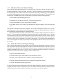
ice accretions on aircraft wings. Shown in Figure 1 is a side view of a typical “noisy” point cloud. In addition to obvious “outliers,” there are points relatively near the surface that are clearly not part of the surface.
It should be noted that the points near the leading edge that appear to be “inside” the airfoil are actually in
2
Figure 1: Noisy point cloud data
“front of” and “behind” the model in this view. Clearly, the data must be filtered before any kind of surface reconstruction can be performed. Manual denoising is relatively easy to perform for two-dimensional
slices but is more difficult for three-dimensional data. One approach is to generate chordwise slices of the
three-dimensional data at different spanwise positions, manually denoise the slices by deleting the outlying
points, and generate a three-dimensional surface by lofting between the slices. Unfortunately, this approach
may adversely affect the fidelity of the surface unless many chordwise slices are employed.
Once the data are denoised, it is necessary to generate a surface representation that is homeomorphic
to and lies in close geometric proximity to the original surface. This is a significant topic in current CAD,
computer graphics, computer vision, and mathematical modeling research. In these applications, a mesh
is often generated using only the scanned data points [6]. In our application we want to generate a surface
upon which a mesh (with a controllable point distribution) can be generated. Simply interpolating a NURBS
surface may not be a good approach due to the potentially oscillatory nature of the reconstruction. Further,
there may be issues related to undersampled data, i.e., insufficient resolution in regions of high curvature. It
seems that many fine scale features (such as roughness and small “feathers”) are likely to be undersampled
by the scanner. Therefore, an additional scale-dependent filtering of the data might also be appropriate. We
are not currently addressing this issue.
In the two approaches discussed below, we consider NURBS representations of the surface. We do
this only because most mesh generation software is based on NURBS representations of the underlying
geometry definition. We now outline two general strategies to generate a NURBS representation from the
point cloud data: a fully three-dimensional approach and a pseudo three-dimensional approach.
3
3.1.1 Fully Three-Dimensional Surface Modeling
In the fully three-dimensional approach we developed as part of this effort, Surfacer was used to “fit” a
NURBS representation to the actual point cloud data. The main advantage of this approach is that the
three-dimensional nature of the ice accretion can be retained. The primary disadvantages are the difficulties
associated with filtering three-dimensional point cloud data and the surface fitting itself. This technique uses
Surfacer to fit a NURBS surface to the iced wing data in conjunction with the following strategy:
1. Extract trailing edge and leading edge curves.
2. Segment the ice wing data into two parts - wing top and wing bottom.
3. Extract side boundary curves of wing top and wing bottom.
4. Fit NURBS surfaces to the wing top and bottom points using the boundary curves and point cloud
data.
This approach is described in detail in the Appendix. We note that obtaining the boundary curves was time
consuming because of the manual interaction needed to clean up the two-dimensional sections. Further, the
three-dimensional point cloud needs to be manually filtered.
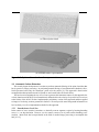
A filtered three-dimensional point cloud and the surface generated using this approach are shown in
Figure 2. There are significant oscillations in the generated surface near the boundary curves. Defining
curves that pass near the tips of the horns and split the upper and lower surfaces into two surfaces each can
reduce these oscillations and reduce the maximum position error by more than 50%. However, this approach
introduces visible slope discontinuities at the surface intersections. These artificial slope discontinuities
occur at critical regions and could pose potentially serious problems for the flow solver as far as accuracy of
the solution.
3.1.2 Pseudo Three-Dimensional Surface Modeling
Choo [9] suggested an alternative approach that is based on lofting two-dimensional chordwise slices of the
data. The primary advantage of this approach is that the needed two-dimensional slices can easily be filtered
to eliminate noisy data points. The disadvantage is that the spanwise resolution is limited by the number of
manually generated chordwise slices. Once the slices are generated and filtered, Surfacer is used to loft a
surface between the chordwise slices using the procedure outline below:
1. Select several spanwise positions
2. Generate chordwise slices of the point cloud at each spanwise station
3. Manually “clean” (filter) the slices to eliminate obviously bad data points
4. Generate a lofted surface between the slices using the two-dimensional sections
5. Generate a NURBS description using Surfacer
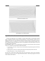
We note that to model a three-dimensional surface with significant spanwise variation, it will be necessary
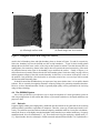
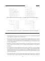
to employ numerous stations across the span. Figure 3(a) shows the manually denoised chordwise profiles
at different spanwise stations and Figure 3(b) shows a wire-frame view of the lofted surface.
4
(a) Filtered point cloud
(b) NURBS surface representation
Figure 2: Fully three-dimensional surface representation
3.2 Automatic Surface Extraction
We recently began development of a routine to perform automatic filtering of the point cloud data that
has its genesis in image processing. In performing manual filtering of two-dimensional chordwise slices,
NASA personnel select only the “innermost” points to be the surface [9]. This approach is based on the
assumption that data points that must be filtered are not located below the actual surface.
We have been investigating the use of level sets to generate this innermost contour. In this approach, the
velocity function used in the level set formulation is defined to drive the velocity of a specific level set to zero
at the surface of the airfoil. We have implemented a preliminary version of this approach and have applied
to images of iced wing sections generated in Surfacer. We now provide some background information on
level set theory as well as implementation details for this approach.
3.2.1 Introduction to Level Sets
In the context of curve (surface) extraction, we basically want to segment a region by locating bounding
curves, i.e., an edge detection. However, we also want to extract a set of points on this bounding curve
(surface). Much work has been performed in the field of medical image processing to accomplish this
task [10–12].
5
(a) Denoised chordwise slices
(b) Wireframe view of lofted surface
Figure 3: Pseudo three-dimensional surface representation
The basic idea behind any level set methods is to perform front tracking, a task normally performed
using a Lagrangian formulation, using an Eulerian formulation. The main advantage is that the level set
approach can be used in two or three dimensions making it possible to perform curve and surface extractions.
Additionally, in the level set approach, it is not necessary to explicitly consider topological changes in the
front. Topological changes occur implicitly in the level set formulation. We now describe how level sets can
be applied to image segmentation.
Level Set Basics: Suppose we have a front that moves with speed in the direction of the local normal
to the curve. In general, may depend on different properties:
1. Local properties of the front - Properties that are determined by local geometric properties of the front
such as curvature.
2. Global properties of the front - Properties that depend on the shape and position of the front.
3. Independent properties - Shape independent properties.
Note that is a function that is neither strictly positive nor strictly negative. We now want to embed the
front position as the zero level set of a higher dimensional function and link the propagation of the front
to the evolution of the function .
6
We start with the zero level set
(1)
Differentiating using the chain rule we obtain
"!$#&%'()*$+-,
Note that the normal to a curve of constant is given by 01
"!$#&74 %'4
/.
(2)
%'3254 %64 so that Eq. 2 can be written as
(3)
where is the velocity component of the front normal to the curve. This is the basic level set equation given
by Sethian [10].
The Front Speed: Typically, the front speed is a function of a constant term, which represents inflation (if
positive) or deflation (if negative) and a curvature dependent term that provides a surface tension effect
8
where <@?
is a user specified constant and =
=A
9;:&<>=
(4)
is the local front curvature given by
"BB"DCEF:&G/"B"DCEHDCB EF#& EIE DCB
CB #& CE
J*K C
.
(5)
How to Solve the Level Set Equation: The level set equation, Eq. 3, is a wave-type equation. What
is important to note is that, like CFD simulations, appropriate numerical solutions of the level set equation
should satisfy an entropy condition. The entropy condition effectively eliminates discontinuities in the front.
The method suggested by Malladi, et. al [11] is to use the first-order upwind scheme given by
QOL P R :&S
"OQL"P R M3N where
% M
TVUW
#eT1U
% `
Tf[c0
#eT\[Q0
TVUWX OQP R YZ% M #T\[Q0]* O^P R Y_%]`
B
a Ob` R 3
C
E
a Ob` R 3
#T\[c0
B
a Ob` R 3
C
C
E
a Ob` R 3
#Tf[c0
C
#T1UW
#TVUW
B
adObM R
C
3
C
NK C
C
NK C
E
a ObM R 3
adObM R
B
3
E
a ObM R 3
(6)
C
where a OQM P R indicates a forward spatial difference and afO^` P R indicates a backward spatial difference of
. Higher-order “Essentially Nonoscillatory” (ENO) upwind schemes were also implemented but did not
significantly alter the results. The initial field is defined using the signed distance function from the initial
level set.
3.2.2 Curve (Surface) Extraction Data using Level Set Methods
This technique is well-developed for pixel-based data (images). The basic idea is to use the level set method
with one modification: the front velocity is driven to zero as it approaches an “edge” in the image. Here
we define an edge to be a significant pixel gradient. Therefore, a straightforward approach is to employ the
modified level set equation
"!$#g/h/()i374 %'4j /.
(8)
7
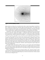
(a) Noisy chordwise slices
(b) Level sets (darkest contour is extracted airfoil surface)
Figure 4: Airfoil surface extraction using level sets
where g/h/(i$ is a speed function that approaches zero as the zero level set approaches an edge. Possible
choices for the speed function include
g/h/(i$
9
9k#l4 %&mFnpokqri$s4
and
g h ()i3
h B P E€
v
t `"u_v w;xzy|{~} x
(9)
(10)
where mFn is a Gaussian smoothing function. Although we are interested only in the zero level set, we are
performing calculations for all of the level sets. Therefore, we need to stop the other level sets when the zero
level set has stopped. The approach used here is the “extension velocity” approach [10]. For a given point
i$ , the speed function is given by the speed function for the point on the zero level set closest to i$ .
For point-based data, the technique is not well-developed. The basic problem is that, for point data,
there is no edge to detect so that the stopping criteria are difficult to define. We have tried several functions
to date (most based on proximity to a point) and none have proved wholly successful.
These difficulties can be illustrated using a simple two-dimensional example. Figure 4(a) shows an
image of a chordwise section of the clean wing generated in Surfacer including noise. Figure 4(b) shows the
extracted level sets with the surface of the airfoil indicated by the darker contour. As is clearly visible in the
figure, the velocity function does not stop at the front in the regions where the pixels are spaced relatively
far apart, i.e., where the pixels do not form an “edge.” Also note the difficulty identifying the sharp trailing
edge. This can be attributed to the relative coarseness of the mesh. A finer mesh upon which the level set
equation is solved would provide a better representation of the trailing edge.
4. Mesh Generation
Mesh generation for an iced wing geometry is a challenging problem. In the sections that follow, we first
discuss some of the issues related to mesh generation. We then outline a procedure to generate a mesh. Next,
we provide images of an example mesh generated using an existing software package. Finally, we conclude
with a discussion of the preliminary efforts related to developing the ICEWING software package.
8
4.1 Issues
From a mesh generation standpoint, there are three driving issues. From the standpoint of efficiency, a
mesh should have: (1) as few cells (faces) as possible, (2) anisotropic mesh refinement, and (3) some degree
of automation. Since we are attempting to compute the solution for a high Reynolds number, viscous flow for
a complex three-dimensional configuration, long computer execution times are to be expected. However, any
potential savings that can be garnered through judicious mesh generation procedures should be considered.
From the standpoint of accuracy, a mesh should have: (1) point clustering in regions of large gradients
and (2) high quality elements (no highly skewed faces or slivers). Obviously, points need to be clustered
in regions adjacent to no-slip boundaries. Additionally, points need to be clustered in regions where wakes
may occur (downstream of ice shapes such as horns). This might suggest using solution adaptive meshes. It
should be noted that sufficient resolution must be present in the initial mesh to capture the phenomenon of
interest. Some control, perhaps manual, is needed to specify initial point placements. From the standpoint of
flexibility, the mesh generation procedure should be able to treat very complex geometries and still produce
high quality meshes. In the next section, we describe a general procedure used to generate a mesh for the
iced wing problem.
4.2 Procedure
Once the geometry representation has been saved in an IGES file, appropriate surface and volume
meshes must be generated. The general procedure we have defined is outlined below:
1. Generate an unstructured triangular mesh on the surface defined in the IGES file.
2. Since we anticipate performing viscous computations, define a wake surface by inserting a plane
downstream of the trailing edge curve of the wing. Then generate an unstructured triangular mesh on
the wake surface. Finally, merge the wake surface mesh with the airfoil mesh.
3. Define side and outer boundaries. Also define flow solver boundary conditions on these surfaces.
4. Generate unstructured triangular mesh on all surfaces.
5. Generate a near-body volume mesh from the surface meshes.
6. Generate a tetrahedral volume mesh in the interior of the domain defined above.
Note that in some mesh generators, the extrusion and void filling steps are seamlessly combined into a single
step. We now consider a sample mesh generated using the SolidMesh [7] software package.
4.3 Example Mesh
To illustrate existing mesh generation software, we have used SolidMesh [7] to generate a mixed element prismatic/tetrahedral mesh starting from an all-triangle surface mesh. SolidMesh was developed by
D. Marcum and A. Gaither at the Mississippi State University Engineering Research Center. The mesh
has approximately 1 million nodes, 6.7 million faces, and 3 million cells. This mesh was used to obtain
a Navier-Stokes solution with the Cobalt flow solver. The results of flow solution are discussed in a later
section.
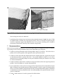
Figure 5 shows the mesh on the surface near ice accretion. Notice the nearly isotropic nature of the
mesh and the potentially inefficient point distribution on the surface. The mesh appears to be of high quality,
however. Figure 6 shows the mesh in the left-side boundary of the computational domain (the additional
lines are part of a frame around the plot). The first thing to notice is that there is no concentration of
points in the wake of the wing. The wake was not included in this demonstration mesh. The mesh extends
approximately 15 chords from the wing in the chordwise and vertical directions. Detailed images of the
9
(a) All-triangle surface mesh
(b) Detail image near ice accretion
Figure 5: Triangular surface mesh (wing lower surface)
mesh in the left boundary plane and right boundary plane are shown in Figures 7(a) and (b), respectively.
Notice the boundary layer mesh clustered near the no-slip boundaries. Figure 8 shows cutting planes
through the mesh on the lower surface of the wing at three spanwise stations. Note that because these are
cutting planes, the connectivity shown in the images does not represent the actual connectivity of the mesh.
Of particular interest in the figure is the boundary layer mesh near the surface. Finally, in Figure 9, we
show a flaw that we located in the mesh in the left-side boundary plane. Notice the widely varying cell sizes
and the apparent collapse of the cells near the boundary. At this time, we are unsure of the precise cause of
the problem. One possibility is the fact that the ice accretion seems to have a severe slope with its normal
directed toward the boundary plane.
It should be noted that SolidMesh may not represent a long-term solution since it is not public domain
software. We are currently investigating alternative software packages for generating unstructured meshes.
However, we have demonstrated that a mesh (of generally high quality) can be generated for the iced wing
using existing technology.
4.4 The ICEWING System
One of the specified first-year objectives was to begin development of a mesh generation system for
iced wing configurations. In the sections that follow, we present the rationale we developed and discuss our
progress to date.
4.4.1 Rationale
It appears highly unlikely that a high quality, multiblock structured mesh can be generated for the iced wing
problem without a prohibitive expenditure of manpower. Therefore, some type of unstructured mesh is a necessity. The problems associated with an unstructured purely tetrahedral mesh for viscous flow calculations–
namely the accuracy of the highly stretched tetrahedra in the boundary layer and the inefficiency of a purely
tetrahedral mesh–are well documented [13, 14]. These deficiencies suggest employing a hybrid mesh [13–
15]. Hybrid meshes have the advantages of both structured and unstructured meshes. In a hybrid mesh, a
10
Figure 6: Left-side boundary of mesh
highly-stretched, near-body mesh is extruded from the surface to capture large gradients in the field variables. Typically, the extruded mesh is generated using an advancing layer scheme. The remainder of the
domain is filled with a tetrahedral mesh. If an extruded surface has quadrilaterals, some type of transitional
element is needed between the extruded mesh and the tetrahedral mesh. Typically, in a hybrid mesh, all the
cells are of standard shapes: triangular prisms and tetrahedra or hexahedra, pyramids, and tetrahedra.
Unfortunately, volume meshes generated using advancing layer methods may have poor quality cells
near convex and concave regions of the geometry. To address this shortcoming of hybrid-type meshes,
several researchers have considered the possibility of using other element types to improve mesh quality.
The resulting meshes, which may contain arbitrary polyhedra, i.e., no restrictions are placed on the number
of edges a face can have or the number of faces a cell can have, have been dubbed generalized meshes [16].
In [17], edge collapse and refinement are used near concave and convex regions of the geometry, respectively,
to improve the mesh quality. In [18], the concept of the generalized prism is introduced to improve mesh
quality by controlling the resolution of the mesh near convex corners. In addition to these operations, the
transition between the near-body mesh and tetrahedral mesh should also be considered. Improved mesh
quality in the transition region can be obtained by having isotropic cells at the extruded mesh/tetrahedral
mesh interface. Edge collapse and face refinement may give the required isotropy in the marching direction
but can spoil the quality in the extruded surface. Therefore, surface cleanup may be required to improve the
quality of the extruded surface.
The added flexibility and potential for higher accuracy in viscous regions make generalized/hybrid
meshes attractive for the iced wing problem. The current interest in hybrid meshes can be ascertained
by a review of the proceedings of the 7th International Conference on Numerical Grid Generation in Computational Field Simulations [19] where there were no fewer than twelve papers on the topic of generalized
and hybrid mesh generation.
We have recently introduced the concept of topological adaptivity [20]. Topological adaptivity implies
using cells that are locally topologically appropriate based on geometric and solution requirements. We now
discuss how we have implemented topological adaptivity for surface and volume meshes. We then conclude
with a discussion of integration issues.
11
(a) Left-side boundary plane
(b) Right-side boundary plane
Figure 7: Mesh on side boundaries near airfoil
4.4.2 Topologically-Adaptive Surface Mesh Generation
We developed an algorithm to convert an all-triangle surface mesh to mixed triangle/quadrilateral surface
mesh. The advantage in performing such a transformation is that the expense of performing a flow solution
strongly depends on the number of faces in a mesh. Therefore, if the number of faces can be reduced without
adversely affecting mesh quality, the cost of a solution can be reduced. The particular algorithm we employ
here combines two triangles if the directions of the surface normals for each triangle differ by less than a
prescribed amount. Figure 10 shows a comparison of the all-triangular mesh generated by SolidMesh with
a mixed-element mesh generated by appropriately combining adjacent triangles. The resulting 37% savings
in cells faces is significant. We have not applied any surface mesh smoothing at this time.
4.4.3 Topologically-Adaptive Volume Mesh Generation
The quality of a mesh generated using extrusion methods may be poor near convex and concave regions of
the geometry. Figure 11(a) shows an example of poor quality cells near a concave region. As this mesh is
extruded, poor aspect ratio cells will develop which will result in “slivers” being generated in the tetrahedral
mesh. One solution to this problem is to employ a change in the topology of the mesh. Edge collapse, as
shown in the Figure 11(b), will stop the generation of poor quality cells and thereby provide the opportunity
to extrude further into the domain and increase the percentage of nontetrahedral elements. Figure 11(c)
shows poor quality cells near convex regions of the geometry. Face refinement, as shown in Figure 11(d),
can improve the quality of the mesh by eliminating highly divergent cells.
Edge collapse and face refinement can also be used to force the mesh to become more isotropic which,
in turn, smoothes the transition to the tetrahedral mesh. However, these operations may lead to poor quality
on the top surface of each layer. Therefore, quality improvement operations should be performed on the
extruded surface as well. The various operations are discussed in the following sections. The terms listed
below are used in the discussion of the quality improvements:

Aspect ratio is defined as the ratio of the largest edge to the smallest edge in a face. This is defined
for each face in the top and base surface of each layer.
12
(a)
(b)
(c)
Figure 8: Cutting planes through the mesh at three spanwise stations (lower surface)


Marching aspect ratio is defined by edge length in the marching direction to the minimum edge
length on the base surface.
Divergence angle is defined for each edge and is defined as the maximum of the in-surface angles
Edge Collapse: The edge collapse operation is performed to improve the quality of the mesh near concave
regions and to force the mesh to become more isotropic. The edges to be collapsed are selected using the
following criteria:


Change in aspect ratio of the faces of the surface mesh before and after extrusion: This ratio is used
to identify the converging cells near non-convex regions.
Marching aspect ratio: This ratio is used to force the faces in the marching direction to become more
isotropic.
The selected edges are given priorities according to the marching aspect ratio and are sorted according to
the assigned priorities. Edge collapse is performed by collapsing the selected edge to a point, typically the
midpoint of the edge. If one of the nodes is a boundary node, then this node is kept to maintain boundary
integrity. The edge collapse process is initiated at the first edge in the list. To avoid performing an operation
that results in an invalid mesh, all of the edges sharing either of the two nodes of the edge under consideration
are marked as non-collapsible edges. After processing the list, the cell connectivity is updated. Edge collapse
results in a generalized cell topology.
Face Refinement: Face refinement is performed to improve the mesh quality near convex regions and to
force the mesh to become more isotropic. Faces are refined according to the number of edges marked for
refinement. The edges are marked for refinement using one of the following criteria:

Divergence angle: This angle quantifies the degree of divergence of mesh faces near convex regions.

Marching aspect ratio: This ratio is used to force the faces in the marching direction toward isotropy.
The selected edges are given priority according to their divergence angles. The selected faces are refined
and cell connectivity is updated. This operation also results in a generalized cell topology.
Extruded Surface Improvement: Edge collapse and face refinement improve the quality along the marching direction. However, these operations do not take into account the quality of the mesh in the extruded
surface. Therefore, the quality of the mesh in the extruded surface may be degraded and improvements in
13
(a) Mesh in left-side boundary plane
(b) Detail of region near mesh flaw
Figure 9: Mesh flaw in left-side boundary plane
the surface are needed. The process is initiated by identifying the minimum angle around each node. The
following steps are performed to improve the surface mesh quality:


Edge collapse: This is done to eliminate small angle cells.
Local reconnection: Poor quality quadrilaterals can be converted into two triangles of better quality
and vice versa.
As the mesh is generated, every step is taken to prevent the generation of negative volumes. The algorithm is designed to give yield triangles and quadrilaterals on the extruded surface. More work is being
performed in the general area of quality improvement. The results of these preliminary efforts are presented
in the next section.
4.4.4 Example Mesh
In this section, we demonstrate the benefits of topological adaptivity for meshes on iced wings. We started
from the all triangle surface mesh shown in Figure 5. We then applied our topologically adaptive surface
mesh algorithm to combine selected triangles to form quadrilaterals. In the final step, we used our topologically adaptive mesh extrusion algorithm to generate a near body mesh. The mesh spacing near the surface
was intentionally chosen to be large so that a clear picture of the extruded mesh could be obtained.
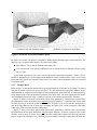
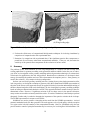
Figure 12 shows a near-body volume mesh (light color) generated by extrusion from a mixed triangle/quadrilateral surface mesh (dark color) without topological adaptivity. A portion of the volume mesh
has been cut away to so that the surface mesh is visible. In Figure 12(a) we note that the mesh quality is
poor in the ridge that runs just aft of the horn. Similarly, in Figure 12(b), we see poor quality cells in the
center ridge of the ice accretion on the leading edge.
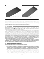
Figure 13 shows a near-body volume mesh (light color) generated by extrusion from a mixed triangle/quadrilateral surface mesh (dark color) with topological adaptivity. As before, a portion of the volume
mesh has been cut away. In Figure 13(a) we note that the mesh quality is improved in the ridge aft of the
horn in comparison with Figure 12(a). Similarly, the mesh quality in the ridge running down the front face
14
(a) All triangle surface mesh
(b) Mixed triangle/quad mesh
Figure 10: Example of simple topological adaptivity in a surface mesh
of the horns is likewise improved as shown in Figure 13(b). It should be noted that we did have some
difficulty extruding much beyond several layers due to mesh crossing in a concave region. We are currently
working to address the problem of mesh crossing using topological adaptivity.
5. Flow Solution
We have generated a Navier-Stokes solution on
in Figures 5-9 using Cobalt* [8] . The
the mesh shown
j
flight conditions were ‚ lY.„ƒ , …†tlGY.„(9Y , and 1lƒ
. The solution required more than 30 hours
of wall-clock time on a 96 processor SGI Power Challenge 3.
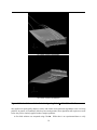
We have investigated the flow field using the visualization package FIELDVIEW [21]. Not surprisingly,
the flow is largely separated over the upper surface. There is also a significant recirculating region on the
lower surface. Stream ribbon traces in the region above the surface aft of the horn are shown in Figure 14(a).
A similar image for the region below the surface is shown in Figure 14(b). Of particular interest in these
images is the three-dimensional nature of the flow separation. Even though the selected ice shape is “mostly”
two dimensional, there are significant spanwise flow components further re-enforcing the need for additional
study of the effects of the geometry modeling aspects of the problem. It should be noted that no serious
attempt has yet been made to establish the validity of the solution. However, these results indicate that it is
possible, using existing technology, to generate a NS solution for an iced wing configuration.
Due to an MPI upgrade in our local system, we have been unable to obtain a HYBFL3D [22] solution.
Additionally, when we attempted to compute a solution remotely using HYBFL3D, the solution diverged
after a few hundred iterations. We attribute this behavior to the flaw in the mesh shown in Figure 9.
6. Assessment of Existing Capabilities
Based on efforts to date, we have arrived at the following conclusions:
1. It is our opinion that Surfacer is a good tool for performing many of the operations needed for basic
geometry modeling for wings with complex ice accretions. It should be noted, however, that all
filtering needs to be performed manually. In our opinion, this is Surfacer’s primary shortcoming.
2. The fully three-dimensional surface modeling approach has some difficulties because the procedure
used to “fit” the NURBS surface produces oscillations in the NURBS description that effectively
distorts the spanwise shape the three-dimensional approach attempts to preserve. The modified procedure, i.e., adding the splitting curves near the horn tips, reduces the position error relative to the
15
(a) Poor quality mesh near concave regions
(b) Quality improvement via edge collapse
(c) Poor quality mesh near convex regions
(d) Quality improvement via face refinement
Figure 11: Topological adaptivity for mesh quality improvement
point cloud data but introduces visible slope discontinuities in the surface. Additionally, this approach
is not appropriate for data that has not yet been denoised.
3. The main deficiency of the pseudo three-dimensional surface modeling approach is that, unless numerous spanwise sections are employed, potentially significant spanwise variations in the ice accretion will not be accurately modeled. Unfortunately, manual filtering of the two-dimensional sections
is a time consuming process.
4. Regardless of the approach used for surface modeling, it seems that some type of automated procedure is necessary to perform filtering. The use of image processing techniques for this purpose is
promising.
5. The mesh generation package SolidMesh was used to generate a mesh for the iced wing configuration. While there was a flaw in the mesh on the left-side boundary of the computational domain,
the mesh appeared to be of generally good quality. However, SolidMesh, which is typical of unstructured/hybrid mesh generators, doesn’t provide the intuitive control for point positioning that is needed
for the iced wing problem.
6. The topologically adaptive surface and volume meshes appear to have promise. However, much work
still needs to be done to improve the quality of the extruded surface. Additionally, the problem of
16
(a) Lower surface of wing
(b) Wing leading edge
Figure 12: Near-body volume mesh without topological adaptivity
front crossing also needs to be addressed.
7. A preliminary flow solution for an iced wing has been obtained using the Cobalt flow solver. While
no validation data is available, the results appear plausible. However, the indicated significant spanwise flow components suggest that additional study of the geometry modeling process should be
performed to determine the sensitivity of the solution to the geometry.
7. Recommendations
Based on the assessments outlined above, we have developed a plan to accomplish the objective of identifying a strategy for the iced wing simulation. Below are the individual steps of this plan:
1. Continue to develop automated surface filtering module using level set theory—We believe this capability will be useful regardless of the approach used to represent the surface.
2. Continue to refine the pseudo-three dimensional surface modeling approach—In particular, develop
an automated procedure to generate data slices. One possible approach would be to use a threedimensional level-set filtering technique on the point cloud data whereby the chordwise slices could
be extracted automatically.
3. Continue to identify software that is available as a long-term solution to the iced wing mesh generation
problem. Several candidates are currently being identified.
4. It is our opinion that, at some point, iced-wing specific mesh generation software should be developed.
What is lacking in current mesh generation software packages is intuitive control of point placement.
However, this effort should be postponed until the utility of computational fluid dynamics simulations
is established for iced wing simulations and a clear understanding of the potential benefits of such a
system is established.
5. Cobalt should continue to be used to generate flow field solutions.
17
(a) Lower surface of wing
(b) Wing leading edge
Figure 13: Near-body volume mesh with topological adaptivity
6. Evaluate the effectiveness of computational fluid dynamics techniques for iced wing simulations by
comparison of computed results with experimental data.
7. Determine, by comparison with experimental data, if the significant spanwise flow components reported here are real features rather than computational anomalies. If they are real, determine the
sensitivity of the spanwise flow components on the resolution of surface model.
8. Summary
The problem of flow field simulation for iced wing configurations is a complex one that severely taxes
existing capabilities for geometry modeling, mesh generation, and flow solution. In the first year of a threeyear effort, we investigated various geometry modeling and mesh generation technologies to evaluate their
effectiveness for application to the iced wing problem. Based on these evaluations, we developed a basic
strategy for attacking the problem and were able to demonstrate the complete process—from geometry to
mesh to flow solution—for a complex iced wing configuration.
Surfacer was used for all geometry modeling activities. Starting from a point cloud representation of the
iced wing surface, we developed a technique to generate a fully three-dimensional NURBS representation of
the point cloud. However, this approach can only be applied to relatively clean data and manual denoising of
the three-dimensional point cloud can be challenging. We also investigated a geometry modeling technique
based on lofting two-dimensional chordwise sections. This approach facilitates manual clean up of the twodimensional section. However, if significant variation of the ice shape occurs in the spanwise direction,
many sections are needed to accurately model the surface. Given these limitations, both techniques perform
adequately. Further study is needed to determine the importance of the spanwise variation in the ice shape.
The NURBS representation is output as an IGES file.
SolidMesh was used to generate a triangular surface mesh from the NURBS representation. A mixed
prismatic/tetrahedral mesh was then generated. The mesh appears to be of good quality with the exception
of a region on the left-side boundary of the computational domain. However, SolidMesh really does not
provide intuitive control of point placement that may be necessary for iced wing flow field calculations. We
18
(a) Upper surface streamlines
(b) Lower surface streamlines
Figure 14: Navier-Stokes solution for iced wing using Cobalt M=0.3, Re=2.0x10 , ‡‰ˆ‹ŠXŒ3Ž
also applied our topologically adaptive surface and volume mesh generation algorithms to the iced wing
problem. In general, we found that, while they have much promise, these algorithms still require more work
before they can be routinely applied to these complex problems.
A flow field solution was computed using Cobalt . While there is no experimental data to verify
19
the solution, it appears reasonable. There is massive flow separation on the upper surface and a significant
recirculating region on the lower surface. The computed results show a significant spanwise flow component.
The effects of the geometry model on these spanwise flow components needs to be evaluated.
20
References
[1] Y. Choo, K. D. Lee, D. S. Thompson, and M. Vickerman. Geometry Modeling and Grid Generation for
”Icing Effects” and ”Ice Accretion” Simulations on Airfoils. P. R. Eiseman, J. Hauser, B. K. Soni, and
!
J. F. Thompson, editors, Proc. 7 International Conference on Numerical Grid Generation in Computational Field Simulations, pages 1061–1070. International Society for Grid Generation, Mississippi
State, MS, September 2000.
[2] W. B. Wright. User Manual for the NASA Glenn Ice Accretion Code LEWICE 2.0. Technical Report
CR-1999-209409, NASA, September 1999.
[3] J. Chung, Y. Choo, A. Reehorst, D. W. Sheldon, and J. Slater. Numerical Study of Aircraft Controlla!„
bility under Certain Icing Conditions. AIAA Paper 99-0375, AIAA 37 Aerospace Sciences Meeting,
Reno, NV, January 1999.
[4] NPARC user’s guide version 3.0, 1996.
[5] Y. Choo. private communication, June 2000.
[6] T. K. Dey, J. Giesen, S. Goswami, J. Hudson, R. Wenger, and W. Zhao. Undersampling and Oversampling in Sample Based Shape Modeling. Proc. IEEE Visualization 2001, pages 83–90, 2001.
[7] D. Marcum. Unstructured Grid Generation using Automatic Point Insertion and Local Reconnection.
J. F. Thompson, B. K. Soni, and N. Weatherill, editors, Handbook of Grid Generation. CRC Press,
Boca Raton, FL, 1998.
[8] R. F. Tomaro, W. Z. Strang, and L. N. Sankar. An Implicit Algorithm for Solving Time-Dependent
!
Flows on Unstructured Grids. AIAA Paper 97-0333, AIAA 35 Aerospace Sciences Meeting, Reno,
NV, January 1997.
[9] Y. Choo. private communication, June 2001.
[10] J. A. Sethian. Level Set Methods and Fast Marching Methods: Evolving Interfaces in Computational
Geometry, Fluid Mechanics, Computer Vision, and Materials Science. Cambridge University Press,
second edition, 1999.
[11] R. Malladi, J. A. Sethian, and B. C. Vemuri. Shape Modeling with Front Propagation: A Level Set
Approach. IEEE Trans. Pat. Anal. Mach. Int, 17(2):158–175, February 1995.
[12] R. Malladi and J. A. Sethian. A Real-Time Algorithm for Medical Shape Recovery. Proc. International
Conference on Computer Vision, pages 304–310, January 1998.
[13] J. A. Shaw. Hybrid Grids. J. F. Thompson, B. K. Soni, and N. Weatherill, editors, Handbook of Grid
Generation. CRC Press, Boca Raton, FL, 1998.
[14] J. A. Chappell, J. A. Shaw, and M .Leatham. The Generation of Hybrid Grids Incorporating Prismatic
Regions for Viscous Flow Calculations. M. Cross, P. R. Eiseman, J. Hauser, B. K. Soni, and J. F.
!
Thompson, editors, Proc. 5 International Conference on Numerical Grid Generation in Computational Field Simulations, pages 537–546. International Society for Grid Generation, Mississippi State,
MS, September 1996.
[15] Y. Kallinderis. Hybrid Grids and Their Applications. J. F. Thompson, B. K. Soni, and N. Weatherill,
editors, Handbook of Grid Generation. CRC Press, Boca Raton, FL, 1998.
21
[16] D. S. Thompson and B. K. Soni. Semistructured Grid Generation in Three-Dimensions using a
!
Parabolic Marching Scheme. AIAA Paper 2000-1004, AIAA 38 Aerospace Sciences Meeting, Reno,
NV, January 2000.
[17] M. Leatham, S. Stokes, J. A. Shaw, J. Cooper, J. Appa, and T. A. Blaylock. Automatic Mesh Generation For Rapid-Response Navier-Stokes Calculations. AIAA paper 2000-2247, Fluids 2000 Conference
and Exhibition, Denver, CO, June 2000.
!„
[18] A. Cary and T. Michal. Generalized Prisms for Improved Grid Quality. AIAA paper 2001-2552, 15
AIAA Computational Fluid Dynamics Conference, Anaheim, CA, June 2001.
!
[19] P. R. Eiseman, J. Hauser, B. K. Soni, and J. F. Thompson, editors, Proc. the 7 International Conference on Numerical Grid Generation in Computational Field Simulations. International Society for
Grid Generation, Mississippi State, MS, September 2000.
[20] S. Chalasani, D. Thompson, and B. Soni. Topological Adaptivity for Mesh Quality Improvement.
!
Proc. 8 International Conference on Numerical Grid Generation in Computational Field Simulations
(submitted), June 2002.
[21] FIELDVIEW User’s Guide Version 6.0, 1999.
[22] R. P. Koomullil and B. K. Soni. Generalized Grid Techniques in Computational Field Simulation.
M. Cross, P. R. Eiseman, J. Hauser, B. K. Soni, and J. F. Thompson, editors, Numerical Grid Generation in Computational Fluid Simulations, pages 521–531. International Society for Grid Generation,
Mississippi State, MS, 1998.
22
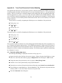
Appendix A:
Truly Three-Dimensional Surface Modeling
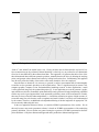
This appendix describes the five steps needed to generate a fully three-dimensional NURBS representation
of iced wing point cloud data. The main objective is to create two distinct surfaces, i.e., the top and bottom
surfaces. These two surfaces have common boundaries at the trailing edge and at an artificial leading edge.
The basic approach is to create a set of curves
that will assist Surfacer in the NURBS definition. These
curves will also be helpful in maintaining ‘ continuity at the common surface boundaries. In the following
report, a bold font is used to identify Surfacer buttons and an italic font is used to identify as the entities
created in Surfacer.
The top surface is created by designating the following curves as boundaries of the point cloud:

Trailing edge curve

Top zmin curve

Leading edge curve

Top zmax curve .
The bottom surface is created by designating the following curves as boundaries of the point cloud:

Trailing edge curve

Bottom zmin curve

Leading edge curve

Bottom zmax curve .
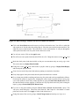
The two surfaces match at common curves at the trailing edge and the leading edge with ‘ continuity. Figure 15 illustrates the notation employed here. The NURBS representation is output in the IGES format so
that it can be imported into most mesh generation software. The unstructured mesh is generated after combining the two surfaces with the mesh generation package. The following steps explains the methodology
for creating the six curves.
A.1 Create the trailing edge curve
The following methodology is employed to create the trailing edge curve.

Import the whole point cloud into the current viewport. Change the point cloud display to scatter
mode if it is not in the scatter mode by going to Display/Point and selecting the scatter button.
Change the name of the point cloud to whole by going to Basic/Change Name.

Orient the view of whole point cloud by using keyboard button F5.

Extract the cross-section of the point cloud at the trailing edge using Point/Cross-section/Parallel.



This will bring up a small dialog box. Click the List button. This will show the all point cloud data
currently visible, i.e., the whole cloud. Select the whole point cloud.
Select the X-direction in the dialog box.
23
Figure 15: Basic Strategy: Generate six curves to define two surfaces


Click on the Start Point button and to return your focus to the main screen. You will see a white line
with a point on it. Decide where the trailing edge is. Place the cursor in this location and click. The
white line moves to that location. This white line is a cross-sectional plane. It will pass through the
whole point cloud and create new point cloud at that cross-section.

Use only one section. Click on the Apply button.

This will create a new point cloud data called Whole SectCld. Change the name to trailing edge cloud
.

Make the whole point cloud data invisible so that you can concentrate only on trailing edge cloud.
This can be done by Display/Point/Invisible
Change the trailing edge cloud scatter mode to polyline mode by going to Display/Point/Display
and selecting the polyline mode.
Zoom in to one end of the point cloud and start panning to examine the cloud data.

If any loops appear in the point cloud, then the point cloud data has to cleaned.



If so, cleanup may include reordering and removing few points and can be accomplished as follows:
Check how the points are organized by changing the scatter mode to polyline for the trailing edge
cloud. If the points are not in order, reorder the points by going to Points/Order/By Direction. Select
Z in the direction box before applying. If still there are any loops then remove the points causing the
loops by going to Points/Modify/Pick Delete Points.

Fit a curve to the point cloud by using the Curve/Create w/Clouds / Fit Free Form option. This
will open a small dialog box. Choose the cloud from the List. Input 50 a the number of control
points and 4 as the order. Click Apply to fit the cloud with the curve.
Change the name of the curve by going to Basic/Change name and entering trail edge curve.
24
A.2 Create the leading edge curve
The following technique is used to extract the leading edge curve.


Make the trailing edge cloud invisible. This can be done using Display/Points/Display and selecting
the trailing edge cloud in the List with the visible button off.

Now put the whole point cloud data with the trailing edge curve in F1 view by pressing keyboard
button F1.

The point cloud data at the leading edge has to be extracted to define the leading edge curve . This
can be done by going to Points/Cross sections/ Parallel. A dialog box opens up. In the dialog box,
select the whole cloud and set the Number of Sections equal to one. Select the Y button in the
Direction box. There will be white plane appearing below the wing where the default start point
exists. To change the start point, click on the Start Point in the dialog box and bring the focus to the
main screen. Place the cursor near the stagnation point of the leading edge and click. The plane will
move to that point.

Click on the Apply button. This will generate point cloud data which will have some points near the
trailing edge region. These points are deleted by Circle Select option.

Put the whole cloud in invisible mode to concentrate on the leading edge cloud. Change the name of
the cloud to leading edge cloud.

Check the point ordering by changing the scatter mode to polyline for the leading edge cloud. Perform cleanup if required.
Choose Fit Free Form from the Curve/ Curve w/Clouds to fit the curve for the leading edge cloud.
Input 50 as the Number of Control Points and 4 as the Order. Click Apply to fit the cloud with
the curve. Change the name to leading edge curve.
A.3 Split the point cloud into two surfaces
 Hide all the data keeping whole point cloud data, leading edge curve and trailing edge curve in the
viewport.


Press keyboard button F1 to orient the point cloud. This will be helpful in splitting the cloud in to
two parts.

Use Circle Select with option Keep Both the Data checked to split the cloud.

Click the cursor on the trailing edge curve and at the leading edge curve and form the loop to break
the cloud.
Change the names of the two resulting point clouds to top and bottom for future reference.
A.4 Create Curves at the Inboard and Outboard Boundaries
This section describes the methodology followed to extract the top zmax curve. The following explains
the method followed to generate the cloud corresponding to top zmax curve.

Put all the clouds into invisible mode except top cloud.

Orient the top cloud to F5 view by pressing keyboard button F5.
25


The point cloud data can be extracted by going to Point/ Cross-section/ Parallel. In the dialog box
select the top cloud from the List. In the Direction select Z. Click on the Start Point and bring
the focus to the main screen. A plane will be displayed on the screen which may not lie on or touch
the cloud. Click at the place where the plane passes across the top cloud in order to get the maximum
number of boundary points and make sure the plane is not too much inside or outside the cloud.

Select one section and click on Apply. This will create a new point cloud data. Change the
name to top zmax cloud temp. One can notice the top zmax cloud temp will not touch the leading edge curve near the far and leading edge intersection.

Now put the top zmax cloud temp into polyline mode and check if there are any loops. If there are
any loops, clean the cloud to remove the loops. In the polyline mode, cleanup the top zmax cloud temp
by removing the points which are causing this if the top zmax cloud temp is not entirely following
the cloud.

After cleaning up the top zmax cloud temp select a small region of top cloud near the intersection
of leading edge and top zmax cloud temp with Circle Select option. Put the top cloud into invisible
mode.

This will create a new cloud. Break the surface into two parts at the turning point by putting the cloud
in F1 (keyboard button) view by using Circle Select with keeping both option.

Fit a surface to both of the new clouds. This can be done by going to Surface/ Create w/ Cloud / Fit
Free Form. In the dialog box select the new cloud created. Set the Order to be 4 and the Number
of Control Points to be 10 in both directions. The Fitting Direction as Best Fit Plane. Keep all the
other data as default.

After obtaining the two surfaces extract the boundary curve of the surfaces which will help in connecting the leading edge to top zmax cloud temp. This can be done by going to Curve/ Create 3D
from Surface / Surface boundary curve. Click on the sides of the two surface boundaries. This
will create the curves. Convert the boundary curves to 50 sample points. Perform cleanup operations
if required to both the clouds. Now add the two small clouds to one and then add this one with
top zmax cloud temp to form one cloud. Change the name of this to top zmax cloud. Before adding
the two clouds check the starting and ending point of the clouds which will be helpful later while
creating the curve. If the ending point of top zmax cloud temp and starting point of newly created
sample points are not consecutive then change the order of the point cloud by Points / Order / Set
Start Point.

Check top zmax cloud with polyline mode and do necessary clean-up if there are any loops.
Create the curve with Curve / Fit w/Cloud / Fit Free Form. Give Number of Control Points to
100 and Order as 4. This will create a new curve.

The curve may not extend all through and hit the leading edge but it will be very close to it.

Change the name of the curve to top zmax curve.
The remaining 3 curves Top zmin curve, Bottom zmin curve and Bottom zmax curve are extracted using the
procedure described above.
26
A.5 Creation of Surfaces
After generating all 6 curves, the first surface (top) is fitted to the top cloud using following curves as
the boundaries:

Trailing edge curve

Top zmin curve

Leading edge curve

Top zmax curve .
The surface can be fitted by giving the number of control points as input or accepting the optimal number
of control points given by Surfacer. The level of accuracy of the description of the NURBS surface can be
varied using the smoothness, tension and standard deviation parameters. One has to be careful in varying
the parameters as the sensitivity to the change in these parameters is high. In the current approach the values
used are 0.75 (tension), 0.5 (smoothness) and 0.5 (standard deviation).
Similarly the second surface (bottom) is fitted to the bottom cloud considering the following curves as
the boundaries:

Trailing edge curve

Bottom zmin curve

Leading edge curve

Bottom zmax curve .
After getting the two surfaces, ‘
continuity is verified at the leading and trailing edge. If they are not
‘
continuous, they can be forced to be so by matching the two surfaces at the interface. Once the two
surfaces are matched, they are saved in IGES format.
The Surface-Cloud difference plot indicates where the NURBS fit does a poor job matching the point
cloud. If the maxiumum error is near the horn tips, one approach for reducing the error is to create an additional curve along the horn tip. This can be done by creating a line by picking two points on top zmin curve
& top zmax curve at the turning points. After generating the line, it can be projected onto the cloud by
Points/ Cross sections/ Project curve on cloud. This will give a set of points on the cloud. Fit the curve
with these points and break the top cloud at the turning point into two clouds. Fit the two surfaces with the
newly created curve as an interface boundary.
27