Download See it at CiteSeerX

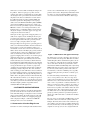
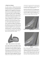
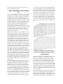
Fast Surface Meshing on Imperfect CAD Models
John P. Steinbrenner, Nicholas J. Wyman and John R. Chawner
Pointwise, Inc., Fort Worth, TX, USA. [email protected]
ABSTRACT
CAD model repair is often a necessary precursor to mesh generation, due primarily to the inconsistencies between the tolerances
used by the designer and the tolerances required by the analyst. This paper presents a method for meshing directly on imperfect
CAD models without needing to repair the model. This is done via a hierarchical grid topology structure that defines a surface grid
by a mesh and by a series of curves defining its boundaries. Curve boundaries are iteratively split and merged based on user-set tolerances, allowing the surfaces to become topologically watertight. Interactive methods to aid in degenerate cases are also
described. Finally, ongoing work for automatic formation of surfaces meshes spanning multiple surfaces is described. This procedure involves agglomeration of surface meshes based on connectivity and bending angle, followed by decimation of surface triangles to remove artifacts from irregularly-shaped CAD surfaces.
Keywords: CAD models, grid generation, automation, interactive, edge curves, surface mesh, splitting, merging
1. INTRODUCTION
As recently as ten years ago, a grand challenge facing mesh
generation developers was the ability to mesh directly on the
geometric models exported by CAD systems. At the time, discrete approximations to CAD surfaces were a reasonable compromise [1][2], but the grid generation community held out
hope that when the original CAD data could be interpreted
within grid software, the primary meshing bottleneck would
be overcome. Implicit in this desire was the (mistaken) belief
that data exported or translated from CAD would be directly
usable by the analysis side of the department, consisting of
watertight surface representations with only pertinent data.
Now that CAD data, either in native form or in a translated
standard form such as IGES [3] or STEP [4], is readily
imported into many grid generation packages, the reality of
CAD is well-understood by the grid community. The challenge has matured from simple interpretation of the data to
clean up and repair of the same data, as the models often arrive
in no shape for analysis. This problem extends far beyond
engineering analysis, with the estimated cost of translation and
repair to be one 1 billion dollars per year [5] in the automotive
industry alone. Indeed, products and corporations have been
formed primarily to address the data problem [6][7].
Some of this problem may be attributed to errors in translation,
software bugs and the fact that there is generally little incen-
tive for a CAD vendor to provide his native files in another
vendor’s format. Blame also points, however, to the designers
constructing the models, who often draft with a set of tolerances well-suited to the preliminary design world, but totally
inappropriate for analysis. Though many industries are aware
of this problem and are conscientiously attempting to rectify it,
legacy files and systems will exist for years to come, and so
grid generators must learn to work with problematic CAD
data.
For analysis purposes, CAD cleanup includes discarding geometric features that are not pertinent to the problem at hand.
Large CAD files often contain information down to the
machining details of the part. Others contain ancillary data
intended, for example, for manufacturing. Neither is pertinent
to analysis, and is better removed from the file or at least hidden from view. Such cleanup generally requires few sophisticated CAD tools, and can be done within many grid generation
packages.
Repair of the CAD file is a more daunting task, because it
requires either the user or the software to fix the file to reflect
the CAD operator’s original intent, whatever that may be.
Some of these errors, especially those dealing at least partially
with topology, may be detected immediately upon import. An
example is a trimmed surface defined in terms of curves that
do not geometrically abut in the way they are topologically
specified. In this example, there is a clear conflict, and many
CAD readers can at least make an intelligent attempt to fix
the problem. When no topology is specified, as in the
example of two surfaces nearly abutting one another (without any higher-order representation), the intended relationship between the surfaces is difficult to ascertain. Such is
the problem frequently encountered with the IGES data
translation specification. Though higher-order topology
entities such as the Manifold Solid B-Rep Object (MSBO)
exist in the latest IGES specifications, these entities continue to be used only sporadically in practice. Generally the
IGES files contain a series of independent surfaces and
trimmed surfaces, each abutting within a tolerance known
only by the designer, so that there appears to be gaps and
overlaps in the collection of surfaces.
tion of a series of mathematical curves representing the
perimeter of the surface. Though many mathematical forms
for surfaces are supported within the IGES specification,
exact conversions exist between all but two distinct types.
CAD repair for these gapped and overlapping surfaces is a
viable, if not complex, means of making the model “grid
generation-ready.” However, it requires the analyst to either
be well-acquainted with CAD-style operations (and software) or to employ 3rd-party software for repair.
This paper will present an approach to generating grids on
surfaces of CAD models that differs from most methods in
that it requires no repair to the underlying surfaces, provided that the errors are due to tolerance inconsistencies. As
will be shown, instead of modifying the geometry and then
creating the mesh, a grid topology will be imposed on the
surfaces, followed by recursive algorithms that connect
gapped/overlapping surface meshes to one another topologically. This grid topology is essentially a data structure
bridge between the basic grid elements (nodes and cells)
and the CAD data (curves and surfaces). Rather than have
the individual grid elements linked directly to the CAD data
for the purpose of CAD error negotiation or feature suppression [8], in this method edges and cells are grouped into
“virtual topology”[9][10] data structures that resemble the
underlying geometry components. The entire automated
surface meshing procedure will first be discussed, followed
by volume meshing techniques, some important interactive
procedures, and finally some ongoing work that promises to
further enhance the quality of meshes formed automatically.
All of the methods herein have (or are being) incorporated
into the Gridgen software [11], a general-purpose mesh generator able to generate 2D, 3D, structured hex and quad, tetrahedral, triangular, prismatic and pyramid cells for
virtually all FEA and CFD applications.
2. AUTOMATED SURFACE MESHING
Triangular surface meshing is currently automated in Gridgen to the extent that users need only select the surfaces to
mesh, with all meshing proceeding based on user-set default
values, described below. The details of this procedure will
be illustrated on the collection of overlapping and gapped
surfaces displayed in Figure 1, taken from an IGES file
defining the front corner of an automobile.
2.1 Construction of Surface Edge Curves
Generation of a surface mesh begins with automatic forma-
Figure 1. IGES surfaces with gaps and overlaps
The simplest type represents a 3D surface by a 2D array of
patches or knots and control points. With this form, which
includes B-Splines, Bezier and Parametric splines, the surface perimeter is defined by the four parametric bounding
curves of the surface. In the more general surface form,
which includes Trimmed and Bounding surfaces (borrowing
IGES terminology), the surface shape is represented again
by a 2D array of data, but the perimeter of the surface is
now defined by a collection of trimming curves, typically
defined in either physical or parametric coordinate spaces,
or both.
For either form, Gridgen automatically constructs edge
curves on each perimeter curve. These new edge curves
(called connectors in Gridgen) are stored as 4th-order Rational Bezier curves, and are defined in terms of the surface’s
UV or curve’s U parametric coordinates. Parametric coordinates are used because surface perimeter curves (lines of
constant U or V ) may be exactly represented by a single
Bezier interval, regardless of the number of intervals on the
underlying surface. The compact form of the edge curves
also makes them easier to edit (adjust individual control
points[11]), and the parametric representation guarantees
that the curve will remain surface-constrained for all subsequent edits.
The edge curves associated with each IGES surface are then
loaded into a surface mesh structure (called a domain in
Gridgen). Each entry in the surface mesh contains the edge
curve number, a direction and a loop number (trimmed surfaces may be defined by several self-closing loops). The two
endpoints of each edge curve are also assigned numerical
values, with each value representing a unique physical location. Hence, each surface mesh will use at most N distinct
edge curve endpoint numbers, where N is the number of
edge curves defining the surface mesh. On the surface mesh
level, then, edge curve endpoints establish topology, in that
they provide the information that links the edge curves.
While the explicit construction of edge curves extracted
from a surface for the purpose of meshing may seem redundant, it is in fact these edge curves that provide connectivity
across neighboring surface meshes. The edge curves ultimately serve as the topological links between all higher
order block grid components, which include structured
(mapped hexahedral), tetrahedral, and prismatic volumes.
Such linkages insure that connectivity is maintained for any
subsequent shape modification or redimensioning of grid
components. Further, edge curves serve as the sole geometric definition for free-form and 2D surfaces (where there is
no underlying geometry).
Figure 2 illustrates a close-up view of the edge curves and
their endpoints (drawn as filled circles) formed on the
perimeter of the surfaces for the example case. Note that
mismatches in the surface geometry are reflected in the edge
curves. Edge curves from adjacent surfaces, though in proximity to one another, are maintained as separate curves. This
also is true for edge curve endpoints. In fact, even if the surfaces abutted perfectly, edge curves and endpoints on adjacent surfaces would be maintained separately after this
initial step.
so that abutting surface boundaries are defined uniquely.
Merging is controlled by two user-set tolerances. The endpoint tolerance ( EndTol ) is the distance at which two
nearby edge curve endpoints will topologically be considered coincident, one replacing the other in all edge curve
definitions. Similarly, the edge curve tolerance ( CrvTol )
is the tolerance at which two edge curves are considered
identical, one replacing the other in the surface mesh definition.
Merging proceeds by comparing all endpoints with all edge
curves, and by repeatedly splitting edge curves at endpoint
locations lying within EndTol of the edge curve. Newtonian search algorithms are used to insure that endpoint-edge
curve splits occurs at the minimum distance between the
two. Since the splitting procedure requires on the order of
2
N comparisons, where N is the total number of edge
curves, extent box comparisons are heavily used, so that the
majority of comparisons between edge curves and endpoints
may be rejected without expensive searches. In addition, all
endpoints and edge curves are assigned to (multiple) cartesian octants that evenly divide the volume. During splitting,
only elements in the same or adjacent octants are compared.
Figure 3 depicts a schematic illustration of the edge curve
splitting procedure. In this figure, solid circles represent the
original edge curve endpoints, and the unfilled circles represent the endpoints added via edge curve splitting.
Figure 3. Edge Curve Splitting
Figure 2. Initial Surface Edge Curves and Endpoints (enlarged)
2.2 Edge Curve Merging
The second step is to identify regions of edge curves that are
in close proximity to regions of other edge curves defined
on neighboring surfaces, and to merge the duplicated curves
In order to suppress the formation of excessive endpoints
due to unnecessary splits, edge curves are not split when the
candidate split location lies within Fac ⋅ EndTol of other
endpoints in the system. This safety factor prevents the phenomenon illustrated in Figure 4. Assume that the 3 endpoints A, B and C on the 3 edge curves are all spaced within
the EndTol tolerance. Without the safety factor above, the
bottom two edge curves would be split at endpoints D, E
and F in the figure. While all of the endpoints would still be
within the tolerance, there would be 3 very short edge
curves formed, namely AD , DE and BF . In addition,
endpoint C would split the bottom edge curve at G , which
would then cause endpoint H and finally I to be formed.
These latter endpoints could easily extend beyond
EndTol from the lower endpoints. This would prevent all
of the endpoints shown from being merged into one, which
would then make it impossible for the edge curves to be
merged properly. By rejecting candidate splits within a certain tolerance, excessively small edge curves would not be
formed. A value of Fac equal to 10, obtained empirically,
is currently used.
curves that are adjacent near one end and diverge on the
other, since there will not be an end point on either edge
curve that specifies the point of separation. In practice this is
not much of a hardship, since adjacent trimmed surfaces
that exhibit this behavior generally are defined by a set of
curves that have already been split. Interactive tools are
available to negotiate these rare cases, however.
Figure 5. Split and Merged Edge Curves
Figure 4. Excessive Edge Curve Splitting
Edge curve splitting is followed by edge curve merging.
Whereas splitting is used to divide partially overlapping
edge curves into adjacent edge curves (through repeated
subdivision), merging is used to identify fully adjacent edge
curve pairs, (within CrvTol ) replacing all instances of
one in the surface mesh definition with the other. For efficiency’s sake, the tolerance test is performed by comparing
the two edge curves at a fairly sparse set of sample points
along the extent of the curves. Though approximate in
nature, this procedure has not yet resulted in an error.
Both the splitting and merging algorithms proceed iteratively until the entire entity list is traversed one time without
further modification. When each is completed, the remaining edge curves will represent a geometrically distinct set,
as illustrated in Figure 5. Perimeter edge curves originally
assigned to a single surface are now replaced by a set of
edge curves that lie either on the boundary of the overall set
of surfaces (used in exactly one surface mesh) or are shared
by neighboring surfaces (used in exactly two surface
meshes). This means that mismatches in the CAD surfaces
have effectively been reconciled without modifying any of
the surfaces, but rather, through repetitive modification of
the edge curves.
The edge curve splitting algorithm is an effective means of
establishing inter-surface connectivity, but there are a few
caveats. For one, the algorithm will not work on two edge
Secondly, generation of a watertight surface mesh with this
procedure requires that the gaps/overlaps in the model data
all be reconcilable with a single tolerance value. This means
that the largest mismatches in the model must be smaller
than the smallest surface or feature. The existence of very
small edge curves (less than the tolerances) on surface
meshes presents no problems, since the small curves reduce
to singularities, and singularities are removed from the surface mesh definition before meshing takes place. If the largest defect is of the same order as the smallest surface or
feature size, however, the best course of action is to reduce
the tolerances by a factor of 2 or more, and try again. All
remaining mismatches may then be reconciled individually
using the interactive tools described later.
2.3 Edge Curve Meshing
The generation of grid points on edge curves during this
process is intentionally bypassed until now so that the splitting/merging procedure is based purely on geometry, and
not on the grid points. The number of grid points assigned
to an edge curve and the distribution of those points is
driven by several user-set default values, described below:
• Avg∆s - the average distance between grid points to be
enforced on the edge curve, used solely to assign a nominal grid point dimension to the edge curve. For example.
an edge curve of length 10 and an Avg∆s of 2 will
result in a grid point dimension of 6 (5 intervals of distance ∆s ).
lem to two dimensions, which is a tractable problem for triangle initialization as well as grid point insertion.
• Beg∆s , End∆s - the spacing constraints to be applied
to the ends of each edge curve (default = no constraint)
• MaxDev - the maximum deviation between the discrete and continuous representation of the edge curve.
Used to add grid points in local regions of high curvature.
(default = no constraint)
• MaxAng - the maximum angular bend between 3 adjacent grid points on the edge curve. Also used to add grid
points in local regions of high curvature. (default = no
constraint)
Since Gridgen merges edge curves common to adjacent surfaces, grid points on the edge curves will usually be defined
in terms of a single surface, which half of the time will not
be the surface on which the mesh is constrained to lie. This
mandates an initial step of closest-point projecting all
boundary points (from edge curves) lying on the surface
mesh’s boundary onto the underlying surface. After meshing, the original boundary points are restored in order to
maintain exact point continuity across surfaces. Since edge
curves are defined only on one of the two surfaces that use
them, all of the error due to surface mismatch appears on the
surface mesh on which the edge curve is not defined.
Though replacing the edge curve with an average of the two
surface boundaries might distribute the error more evenly, it
would increase the number of projections required, as both
surfaces using the edge curve would require projection to
the geometry. The sparse form of the edge curve representation described earlier would also be lost, since the curve
would no longer be defined by a linear parametric curve.
An edge curve is meshed by first having a number of grid
points assigned to it, calculated from the Avg∆s value.
Next, grid points are distributed along the edge curve using
a 2-sided stretching function based on the hyperbolic tangent function [12]. The Beg∆s and End∆s values, if
applied, control the degree of clustering. Finally, the grid
point distribution is modified by recursively inserting grid
points where the MaxAng and MaxDev criteria are
violated. The resulting distribution is then stored in spline
form to facilitate subsequent editing of the edge curve shape
and/or distribution.
2.4 Surface Meshing
Surface triangulation may proceed in either 2D or 3D in
Gridgen. In each mode, the perimeter of the region to be
meshed is first defined by a string of edge curves. In 3d
mode, the geometry surfaces on which the mesh will be
constrained to lie are also specified. As the name suggests,
all calculations are done using 3D space coordinates, and
each inserted or adjusted node must be projected (using a
closest point search) onto the defining surfaces. 3D mode’s
most compelling feature is that it allows individual meshes
to be formed that lie across multiple surfaces. Since the first
step of the surface meshing is the initial triangulation of the
boundary points, the 3D mode is limited to surface meshes
on which the collection of edge curve points form a reasonable gross planar approximation (automatically calculated
from a least squares planar fit of the grid points). In general,
as along as all surface normals lie in the same half-plane relative to the planar approximation, the meshing will proceed.
For regions such as bodies of revolution the 3D mode
breaks down, because widely varying normals make initial
triangulation of the boundary points impossible, and
because the closest point algorithms could potentially move
grid points to the improper side. In an interactive environment, however, it will always be possible to divide the
region into quasi-planar subregions, each spanning multiple
surfaces, and so the 3D mode remains a powerful interactive
tool in Gridgen.
For automatic surface meshing, however, we rely on the 2D
meshing mode, where both boundary and interior grid
points are defined in terms of the parametric coordinates of
a single underlying defining surface. Working primarily
with the parametric coordinates reduces the meshing prob-
Particular care must be taken when projecting boundary
points onto a periodic trimmed surface such as a body of
revolution, because a closest-point projection is equally apt
to return a point on either side of the periodic seam. Because
the triangulator uses parametric data, only one of these two
values is proper. In these cases, Gridgen uses an iterative
procedure to determine the proper side of the periodic surface for each grid point, based on an algorithm that minimizes the computational area of the bounded region.
By meshing in the parametric space of the surface, the quality of the resulting grid becomes excessively dependent on
the parametrization of the surface. To reduce the influence
of the parametrization, a variety of parametric field distortion methods have been proposed [13][14]. In Gridgen, a
transformation is used that maps the 2D rectangular parameter space of the surface to a (possibly) sheared and scaled
2D space that mimics the average partial derivatives in 3D
in both magnitude and included angle between them. This
mapping is a very accurate representation when the ratio of
∂r ⁄ ∂u to ∂r ⁄ ∂v is relatively constant and the included
angle between the two partial derivatives is relatively constant across the surface.
Surface mesh refinement (grid point insertion and local retriangulation) beyond the initial triangulation (which triangulates the boundary points without inserting interior
nodes) is applied to any triangle that violates penalty functions based on the criteria below:
• MinTri - the minimum allowable triangle size, used to
prevent refinement overflow. (default is derived from the
minimum boundary size)
• MaxTri - the maximum allowable triangle size, the
main driver of node insertion. (default is derived from the
maximum boundary size)
• MaxDev - the maximum allowable deviation between
a triangle centroid and its underlying surface, used to
refine in high curvature areas.
• Decay - A triangle target size field is computed from
the boundary grid point distributions and this user-set
decay factor. Values of this factor control the degree of
influence of boundary spacing on the interior triangle cell
sizes.
The resultant surface mesh is smoothed and diagonal
swapped at interim stages of refinement based on additional
default values controlling relaxation factor. Smoothing is
administered in 3D, and is then transformed to 2D coordinates using the 3D shift and the local partial derivatives at
the original position.
The overall product of this automated procedure is a set of
node continuous triangular grids that span across a collection of possibly non-continuous surfaces, as depicted in Figure 6.
Figure 6. Triangulated Surface Meshes
3. VOLUME MESHING
When the automated procedure above is used to generate
point-continuous surface meshes across imperfect geometric models, the assembly of the surface meshes into closed
surfaces, and the subsequent tessellation of the regions’
interior into tetrahedra is a straightforward and nearly automated task. In the cases where the surface meshes created
automatically above form watertight closed surfaces, the tetrahedral mesher can be applied after only a few user inputs.
Total automation is not yet available for these cases because
Gridgen is a multi-block code, allowing the user to divide
the overall tet grid into any number of smaller “blocks”
(partitions of the total grid), and the user is required to prescribe which surface meshes belong to the block under construction.
The final step of grid generation involves selecting the
blocks to be meshed, setting a variety of default values anal-
ogous to the surface parameters described earlier, and
invoking Gridgen’s tet mesher [15]. The resultant tetrahedral mesh may then be exported in the format of any of the
leading CFD and FEA packages, including Fluent, CFX,
Star-CD, PATRAN and NASTRAN.
4. INTERACTIVE TOOLS
As described above, significant automation has been added
to Gridgen’s feature list, but it is the interactive tools that
allow users to proceed when confronted with problems that
have not or cannot be automated. Two of Gridgen’s more
powerful interactive tools, each of which is best used in conjunction with the automated surface mesher, are described
in this section.
4.1 Assembling Closed Surfaces
The assembly of individual surface meshes into watertight
closed surfaces described above proceeds via a low-level
user-interface designed for topologically complex cases,
such as manifold surface connections (more than two surface meshes sharing a single edge curve). This same userinterface is implemented in several locations in Gridgen: for
agglomeration of multiple surface meshes into a single
mesh, for assembly of surface meshes into the six faces of a
structured block, and for assembly of structured and
unstructured surface meshes to be extruded into hexahedral
and prismatic volume meshes [16].
The 3D region to be meshed will always have a closed surface boundary representing the region’s exterior, and frequently will have a number of inner closed surfaces
boundaries. Each of these closed boundaries will generally
be defined by a collection of watertight contiguous surface
meshes. Since it is not assumed in Gridgen that any or all
existing surface meshes belong to a particular region, closed
boundaries must be formed interactively via user specification of the constituent surface meshes. During assembly,
each added surface mesh is linked at the edge curve level to
exactly one other surface mesh in the current closed surface
(under development). As surface meshes are added, the current boundary of the developing closed surface (edge curves
that are not yet linked to another surface mesh) is displayed
prominently for easy identification. Surface meshes are
added to the closed surface either by selecting them individually, by adding all surface meshes adjacent to the current
collection, or by selecting multiple (possibly all) surface
meshes simultaneously. In the latter case, Gridgen iteratively attempts to attach all selected surface meshes to the
growing closed surface, until all surface meshes have been
added or there remains no more viable linkages. In the
instances where the newly added surface mesh may attach
to the face in more than one way, the user selects the proper
linkage from a toggled list of all possible linkages. This
allows manifold surfaces, such as a wing geometry followed
by a wake of zero thickness, to be assembled properly.
4.2 Edge Curve Merging
Successful closed surface assembly is predicated on all surface meshes connecting to one another properly, which in
turn depends on all new edge curves being split and merged
properly and adequately. As described earlier, this is not a
problem as long as the maximum gaps and overlaps in the
underlying surfaces are smaller than the nominal triangle
edge size and are smaller than the smallest geometric features in the geometry. For more problematic models, however, it will not be possible to specify a single EndTol
and EdgTol combination that will reconcile all problems,
and the edge curve merging needs to be applied on a per
case basis. Interactive edge curve merge tools are available
from several locations within Gridgen, but none are as
effective as within closed surface assembly. Here, the user
can begin to assemble the necessary surface meshes into the
closed surface in the usual way, and may reconcile any
unmerged edge curves along the way until the closed surface is fully assembled. Specifically, the user may merge
edge curves and/or their endpoints, and may split edge
curves by selecting the appropriate button and entering a
tolerance. All edge curve, endpoint, or edge-endpoint pairs
lying within the given tolerance will be displayed, the user
then selecting the pairs that truly need to be merged or split.
To insure that only appropriate pairs are selected, the user
may limit the candidates to edge curves defined only in a
single surface mesh, to edge curves lying on the boundary
of the developing face, or to those edge curves that do not
lie on the interior of the developing face. These masks allow
the user to navigate and quickly reconcile the unmerged/
split edge curves in the face under assembly.
ately indicates two gapped regions. By selecting a gap tolerance of twice the original tolerance, each of these gaps may
be interactively selected and merged, rendering the collection of surface meshes watertight. (Figure 9).
Note that it is usually dangerous to select global meshing
tolerances that are on the order of the smaller length scales
of the geometry detail. In this example, the gap in surfaces
was as high as 30% of the length of nearby edge curves. If a
tolerance near 100% of the edge curve length had been
selected, the edge curve would be represented in the mesh
by a single point, which compromises the geometry.
Figure 8. Interactive Display of Unmerged Surface
Edge Curves
Figure 7. Meshed Surfaces on Exterior Mirror
As an example, consider the geometry in Figure 7, which
depicts a collection of surface meshes around an automobile
exterior mirror. Using a grid point spacing of 0.1% of the
nominal model size, and using a EndTol and EdgTol
equal to 0.02% of the model size, the majority of the neighboring edge curves are automatically merged during surface
mesh construction. Where surface meshes do not connect is
visually difficult to discern on this model (more so on larger
models), at least until the surface meshes are linked to one
another during closed surface assembly. Figure 8 illustrates
Gridgen’s interactive display of unlinked edge curves on the
boundary of the developing closed surface, which immedi-
Figure 9. Surface Meshes After Edge Curve
Merges
When a suitable meshing tolerance is not known beforehand, the recommended procedure is to use a low tolerance,
and interactively merge the remaining edge curve pairs not
caught with the input tolerance. Since an input tolerance
that is too small will shift the merging burden entirely to the
interactive side, it is sometimes necessary to choose input
tolerances iteratively, perhaps doubling the tolerance each
time until the automated merging is triggered in all of the
benign regions of the model. The remaining merges may
then be reconciled interactively.
5. MODEL-INDEPENDENT SURFACE MESHING
The edge curve in Gridgen has been shown to the enabling
topology element that allows a collection of physically disjoint surfaces to be meshed in a grid point-continuous manner. While robust enough to be automated, the procedure
suffers from the feature that all surface boundaries are captured in the final surface mesh. Inspection of Figures 5 and 6
reveals that many of the edge curves of Figure 6 are visible
in Figure 6. While edge curve grid point capturing is necessary when a surface mesh is intentionally bounded at a
sharp edge in the geometry, it is not desirable in the
instances when a large number of surfaces are used to define
a relatively benign piece of geometry. An ideal surface mesh
is not influenced by the number, geometric extents or
parametrization of the surfaces defining its geometry, but
only by the geometry itself.
Numerous researchers have devised techniques for creating
model-independent meshes [17][18]. In Gridgen, this problem is currently remedied to a certain extent using surface
mesh agglomeration tools and repeated application of the
surface triangulator. All surface meshes to be joined into a
larger mesh are first selected using the closed surface
assembly interface described earlier. These surface meshes
are then agglomerated, and the triangulating attributes of the
new surface mesh is modified so that it is attached to all
geometric surfaces of the constituent surface meshes. The
triangulator is then invoked, this time in 3D, and grid points
are inserted and diagonals are swapped in the usual manner,
with triangle nodes free to migrate across all of the selected
surfaces. After node insertion and smoothing, the edge
curve outline in the surface mesh will tend to dissipate.
Though the mesher is invoked in 3D geometric coordinates
rather then in surface intrinsic variables, the limitations typically associated with the 3D mode described earlier will no
longer be present. This is because the mesher will be refining existing triangles (rather than refining very coarse initial
meshes with widely varying node normals), where the triangle normal and underlying surface normal will always be
close enough to compute the proper node location (via normal projection).
In the current implementation, triangle nodes inserted into
the surface mesh interior remain with the surface mesh for
all subsequent refinements, smooths and swaps. For the
automated surface mesher, then, there is no mechanism
implemented to remove excessive node clustering. For this
reason, triangle decimation functions are currently being
implemented into Gridgen. In decimation, triangles sharing
a given node are retriangulated with the node removed if
none of the new candidate triangles violates the refinement
criteria described in Section 2.4. In other words, a node will
be removed from the mesh if the new triangles replacing the
original will not require that node to be re-inserted. An
example of decimation is illustrated in Figure 10. At the top
is a joined surface mesh created from 70 individual surface
meshes. The triangulator was not invoked for this example
so that the original edge curves would remain prominent. At
the bottom is the same mesh after decimation, where all artifacts of interior surface boundaries have been removed.
Work is underway to implement the surface mesh agglomeration and mesh decimation functions into the automated
procedure described in Section 2. For agglomeration, two
surface meshes will be joined as long as they uniquely share
a common edge curve and the triangle bending angle across
the edge curve seam lies under a user-set maximum threshold.
Figure 10. 70 agglomerated surface meshes
before (top) and after (below) mesh decimation.
6. CONCLUSIONS
In this work a straightforward and robust procedure for the
automatic construction of watertight surface meshes on
CAD surfaces containing gaps and overlaps of various
degrees has been presented. This method meshes across
geometry imperfections by establishing a grid topology
hierarchy consisting of edge curves and surface meshes,
where edge curves are 1D curves defined on the boundaries
of the surfaces, and surfaces meshes are structures containing topological connection data as well as grid points and
triangles. Through recursive splitting and merging of the
edge curves, originally mismatched surface meshes may be
rendered watertight.
Further, work is ongoing that will allow the imperfect CAD
surfaces to be meshed independently of the number and
character of the underlying surfaces. This will be accomplished through automated surface mesh agglomeration and
mesh decimation. A combination of decimation, mesh
smoothing and diagonal swapping will be used to remove
artifacts in the agglomerated mesh formed by irregularly
shaped surfaces or surfaces of differing length scales. The
result will be a uniform surface mesh based on geometry
alone. This new procedure will further streamline the grid
generation process, allowing the user to go from CAD
model to volume mesh with only a few default settings and
decisions.
7. REFERENCES
[1] Luh, R. C-.C., Yip, D. and Pierce, L.E., “Interactive
Surface Grid Generation,” Numerical Grid Generation in Computational Fluid Dynamics and Related
Fields, proceedings of the 3rd International Conference, Barcelona, Spain, 03-07 June, 1991, ISBN 0444-88948-5.
[2] Eiseman, P.R., Cheng, Z., and Häuser, J., “Applications
of Multiblock Grid Generations with Automatic Zoning,” Numerical Grid Generation in Computational
Fluid Dynamics and Related Fields, proceedings of
the 4th International Conference, Swansea, Wales, 0608 April, 1994, ISBN 0-906674-82-4.
[3] Reed, K., “The Initial Graphics Exchange Specification (IGES),” NISTIR 4412, National Institute of Standards, September, 1991.
[4] Owen, J., “STEP-An Introduction,”, Information
Geometers Ltd., 47 Stockers Avenue, Winchester,
England, 1993.
[5] Brunnermeier, S.B., and Martin, S.A., “Interoperability
Cost Analysis of the U.S. Automotive Supply Chain,”
Research Triangle Institute Project Number 7007-03,
March, 1999.
[6] “CAD Model Repair,” in Plastics Product Review,
October/November, 1999.
[7] Butlin, G. and Stops, C., “CAD Data Repair,” Proceedings of the 5th International Meshing Roundtable,
1996.
[8] Mobley, A.V., Carroll, M.P., and Canaan, S.A., “An
Object Oriented Approach to Geometry Defeaturing
for Finite Element Meshing,” Proceedings of the 7th
International Meshing Roundtable, 1998.
[9] Sheffer, A., Blacker, T.D., Clements, J., and Bercovier,
M., “Virtual Topology Construction and Applications,”
Geometric Modeling Theory and Practice, pp. 247259, Springer-Verlag, 1997.
[10] Sheffer, A., Blacker, T.D., and Bercovier, M., “Steps
Towards Smooth CAD-FEM Integration”, Numerical
Grid Generation in Computational Fluid Dynamics
and Related Fields, proceedings of the 6th International Conference, Greenwich, U.K., July, 1998, ISBN
0-9651627-2-9.
[11] Gridgen User Manual, Version 13.3, Pointwise, Inc.,
Fort Worth, TX, 2000.
[12] Vinokur, M., “On One-Dimensional Stretching Functions for Finite-Difference Calculations,”, NASA CR3313, 1980.
[13] Chen, H. and Bishop, J., “Delauney Triangulation for
Curved Surfaces,” Proceedings of the 6th International
Meshing Roundtable, 1997.
[14] Farouki, R.T., “Optimal Parameterizations,” Computer Aided Geometric Design, Vol. 14, pp. 153-168.
[15] Steinbrenner, J.P., Chawner, J.R., and Matus, R.J.,
“Evolution of Gridgen’s Data Hierarchy to Unstructured Grids,” Numerical Grid Generation in Computational Fluid Dynamics and Related Fields,
proceedings of the 6th International Conference,
Greenwich, 06-09 July, 1998, ISBN 0-9651627-2-9.
[16] Steinbrenner, J., Wyman, N. and Chawner, J., “Development and Implementation of Gridgen’s Hyperbolic
PDE and Extrusion Methods,” AIAA paper 2000-0679,
Reno, NV, January, 2000.
[17] Marcum, D.L., and Gaither, J.A., “Unstructured Surface Grid Generation Using Global Mapping and Physical Space Approximation,” Proceedings of the 8th
International Meshing Roundtable. Lake Tahoe, CA,
10-13 October, 1999.
[18] Inoue, K. et al., “Clustering a Large Number of Faces
for 2-Dimensional Mesh Generation,” Proceedings of
the 8th International Meshing Roundtable, Lake Tahoe,
CA, 10-13 October, 1999.