1
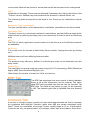
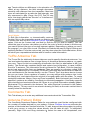
...a Customer Friendly Company ComStudy Version 2.2 For Microsoft Windows User Manual 2.2.6 Contacting RadioSoft Telephone 706.778.6811, 706.778.6812 (FAX), 888.RADIO95 (Orders, USA) 101 Demorest Square, Suite E, Demorest, Georgia 30535-6044 USA (Mail) [email protected] (email) Contents Installation First Time Licensing Requirements Starting ComStudy What ComStudy Does New Users Mapping Transmitter Information Site Information General Tab ERP Tab Radio Contours Tx/Rx Antenna Tab Comments Antenna Pattern Editor Underlays Terrain Height Field Strength Transmitter Matrices Area Reliability Differential Studies Interference TSB-88 Interference Area Reliability w/ Interference Shadow Depth Population Land Use/Land Cover Overlays Vectors Text Cities Callsigns Labels Scale Obstacles Path Profile Views Pull Down Menus Site Fields Path Assignment List Path Values 3D Viewer 1 1 1 2 3 3 3 4 5 5 6 6 6 7 7 8 8 9 9 10 11 11 11 12 12 13 13 14 14 14 15 15 15 16 16 17 17 17 How-To Create a New Site Search the Database for an Existing Site Create a Matrix Study Import Studies from ComStudy 1.5 Import Drive Test Data 19 20 21 22 22 Printing 23 Templates Defaults Saving & Applying 24 24 Tools Map Controls Map Properties Color Palettes Cursor Tools 25 25 25 26 Technical Information Propagation Models Resolution User Files & Databases Frequency Bands Glossary Status Codes Field Units Conversion Formulas 26 27 27 28 28 32 34 35 Copyrights and Trademarks RadioSoft is a registered trademark of Mountain Tower, Ltd. Microsoft is a registered trademark and Windows is a trademark of the Microsoft Corporation. ComStudy is licensed only for use in accordance with the accompanying license agreement. No part of this manual may be reproduced in any manner whatsoever without the written permission of Mountain Tower, Ltd. Except as specifically provided in the license agreement, you may not reproduce the software without the written permission of Mountain Tower, Ltd. Liability: It is understood and agreed by the user that RadioSoft is expressly held harmless of any and all liability, whether incidental or consequential, from use of this software product and its output, whether electronic or printed. Installation First Time ComStudy V 2 is supplied with an installation program, usually on CD-ROM, which performs the following tasks: 1. Registers your name and Company or Organization 2. Extracts ComStudy Programs 3. Extracts ComStudy support files 4. Configures ComStudy Mapping files This Configuration is done in Window's Registry. You may modify this later using the menu item File|Configuration. Note for NT or 2000 users: since ComStudy requires write access to the registry, you will need administrative privileges. How to Do It Place the CD-ROM into the appropriate drive. Use the Auto-Run popup window, or from the Window's Start menu, choose Run, type "x:setup" where "x" is the drive into which the install medium is placed, and press ENTER. The Setup Installation program will ask you to enter your name and company affiliation (if any). If it has been previously registered, it will ask if you are the person to whom the software is registered, and then install as above. Registering The first time you run ComStudy, you'll immediately be presented with our Registration screen. Click "next", and you'll see a serial number, which is unique to your particular computer and installation of ComStudy. Call or e-mail us with this number, and we'll return a user's key to get you on your way. Additional Files ComStudy normally is shipped with Terrain or other database files on separate CDROM's. There is a setup file for each one on the ROM, and you should install these also. Upgrades If you're upgrading ComStudy, you'll have an executable upgrade file (with a name like CS240004.EXE) Run the program by double clicking on it in Explorer or typing its path and name in Start|Run, and it will check to ensure your old program is properly registered, replace it, and auto-register your new upgrade. Licensing All copies of ComStudy are required to be licensed to a single user. If you are not sure whether you are licensed, or if you are not the company representative of your company for whom the license is valid, please contact RadioSoft at 706.778.6811 or by e-mail at [email protected]. Requirements Operating Sys tem Support ComStudy is built for Windows 32 bit systems only. Support for Windows 3.1 has been dropped, including 3.11 with 32 bit extensions. Platforms supported are Windows 98, Windows 2000, Windows NT, & Windows XP (by Microsoft). Windows ME will run ComStudy, but its performance and operability with other applica1 tions may suffer. To run ComStudy with adequate performance, the following is necessary: Hard Disk System ComStudy uses save, swap, and print files that can become quite large. A minimum of 1 GB to 3 GB must be available for installation and the running of ComStudy. Sizes of ComStudy databases vary between 500 MB and 2 GB. Both SCSI and ATA/IDE hard drives are suited for ComStudy. With its heavy demand on disk systems it is best to have a fast drive (11 ms average access or better). CD-ROM System If ComStudy is run using the CD drive, a fast CD drive (at least 12X) is required. Memory ComStudy may run very slowly in computers with less than 64 MB of memory, especially with studies involving many transmitters. NT or 2000 may require even more memory for adequate performance. We recommend at least 128 MB of RAM, and 512 MB for studies with large numbers of transmitters. Processor Many calculations within ComStudy are processor dependent. A Pentium or AMD 200 MHz CPU is a minimum. Recommended 600 MHz for good performance. Video ComStudy requires high color (16 bit) or true color (24/32 bit) modes (at least 65,536 colors), so video cards with less than 4 MB of Video RAM are not supported. Though ComStudy will run in 800 x 600 mode, we recommend at least 1024 x 768, with a 17" or larger monitor for everyday use. Network We do not recommend network connections for ComStudy. Unlike many database programs, ComStudy uses large amounts of I/O for such tasks as terrain loading, which makes it poorly suited for server or client-server operation. This caution also applies to sharing terrain data files only, which would burden most LANs. Furthermore, ComStudy itself may be used on a network only in compliance with the supplied license agreement. Sharing of saved studies among licensed users over networks, via Internet or email is expressly permitted. If studies are published via pictures on the Internet, RadioSoft requests attribution. Internet RadioSoft may offer data updates, program upgrades, new or modified support files, and news that can be downloaded from our web site at www.RadioSoft.com. ComStudy may not be run in any way that provides user access to its operating functions on the Internet. Windows Conventions Most accepted Windows operations are used in ComStudy. There are many ways to navigate menus or perform tasks. Point-and-click or keyboard shortcuts apply throughout the program. ComStudy uses standard Windows printer and display drivers. Starting ComStudy ComStudy may be started in several ways, after it has been successfully installed. Choose Start|Programs|ComStudy|ComStudy20 or create a desktop icon for ComStudy. If ComStudy cannot be found in the programs menu, reinstall or call us for help. 2 What ComStudy Does New Users Most uses of ComStudy involve plotting signals from one or more transmitters. Therefore, the two things necessary to create a study are 1) Create a map on which to display the data. ComStudy requires a map as a "container" for all other data. Maps may be moved, resized, etc. 2) Search for or define one or more transmitters, which is done in the Transmitter Information window. ComStudy can read in data from all available FCC (and many foreign government) databases. These data are separated by type of service, so you must specify which service (Broadcast: AM, FM, TV; Land Mobile: VHF High, UHF, Microwave etc.) you wish to use. This is also true when defining your own transmitters, as contour types and other information change depending on service desired. Mapping There are two groups of layers in ComStudy's maps: Underlays (colors which go in the background of the map) and Overlays, which are drawn on top of the Underlay, if any. Examples of Underlays are Field Strength and Bitmaps. Examples of Overlays fall into two categories: Text and Labels, and Linear features such as Roads, Country or County borders etc. The other parts of a map are: Title bar This displays the Map Title. Map Titles may be imported from existing files, or assigned when you save a study. Status Lines The status line (at the bottom of the program) shows information at the cursor location, if it's on the map. You'll see latitude, longitude, terrain height and land use. If field strength matrices of various kinds are available, information about fields will also be displayed. Transmitter Information Managing Transmitter Information is one of the two central tasks in ComStudy (the other is mapping). To view the Transmitter Information window, you must have a map in which to define your study. The Transmitter Information window has the following functions: 1) Choosing which Frequency Band in which to operate. 2) Searching for or defining new transmitters. See How-To Search the Databases for an Existing Site. 3 3) Showing a list of transmitters for selecting and editing. 4) Choosing what information about each transmitter to show. 5) Editing transmitter contour values, types and displays. See Radio Contours . 6) Defining and calculating transmitter matrices. See How-To Create a Matrix Study. 7) Selecting Underlay types (switching views). Site Information General Tab The General tab contains basic site information: Call Sign The call sign of the site, or its label. This normally appears on the map. Latitude/Longitude The geographical coordinates of the site. These may be entered in Degrees, Minutes and Seconds. Southern latitudes and Wes tern longitudes must be preceded by a minus sign or followed by and "S" or "W". ComStudy can usually identify any other methods of coordinate entry, including decimal ("73.1075") or just typing six or seven numbers ("1110532" becomes 111-05-32 W). Enter NAD 83 (WGS-84 outside the United States), except for domestic FM, AM & TV use NAD 27. ERP Calculated effective radiated power. This field will be updated when an ERP or Antenna Tab is accessed. Frequency The site’s frequency in megahertz (MHz). AM sites are in kilohertz (kHz). Some bands (TV, for example) have channel numbers also. City The City or area to which the transmitter is licensed. State, Country The places in which the City is located. Format (AM/FM only) The program content of the broadcast station. Elevations Elevations are shown both as calculated by ComStudy from its terrain databases and (where known) as retrieved from FCC or other transmitter databases. Antenna AGL The antenna’s height above ground level (not sea level). If known, the elevation of the center of the antenna is preferred. Ground Elev The ground elevation of the site at the given location. This is looked up by ComStudy from terrain databases and shown to the right of the field. Actual elevations are often higher than this value and should be used where known. RCAMSL The antenna’s Radiation Center Above Mean Sea Level, or the ground elevation plus the antenna’s AGL. This must be higher than the ground elevation looked up by ComStudy, 4 or the matrix fields will be incorrect, as the antenna will be assumed to be underground. HAAT Height Above Average Terrain may be adjusted if necessary by clicking the button in the "Terrain" column. Radials may be truncated at the shoreline, national border, etc. The remaining fields are specific to the band in use. Some are for interference calculations:. Modulation Type (Land Mobile) The type (and deviation) of the transmitter’s modulation, selected from the list provided. Time Delay Shift This field, used only in simulcast interference calculations, permits shifting a single transmitters phase (by altering its delay time in microseconds) in order to move an interfering area. ARN The FCC (or other) application record number of a site from one of ComStudy’s transmitter databases MLS Color The current color for this site in Most Likely Server studies. Change the color by clicking on it. AM Band users will have differing fields and tabs: Efficiency The antenna array efficiency, defined in millivolts per meter at one kilometer from the array center. Pattern Type This describes the overall antenna system using the FCC terminology: DAN (Directional Night), NDD (Non-Directional Daytime), etc. Other fields, like number of towers for a DA, are obvious. ERP Tab The ERP tab calculates how much power is being radiated. Some or all of this inform ation can be entered. The calculated ERP will be posted from this tab into the General Tab ERP field. The fields all use losses (or gain, for the antenna) in dB. The antenna gain field is imported from the Antenna tab. Contours Tab A contour is a single polygon (usually circular) which approximates the limit of coverage at a particular field strength. Contours (other than AM) are usually calculated using HAAT. Since the calculation of Average Terrain usually stops at 15 or 16 kilometers, Contours are only an approximation of coverage, rather than a true Matrix. Since Aver5 age Terrain defines no difference in the elevation of a radial, at any distance, the field strength decreases smoothly with distance from the transmitter. Most contours are calculated for a particular field strength, usually expressed in dBµ. Some, like FCC Part 22 contours, are simply defined as "Service" or "Interference", with no explicit dBµ value. How It Works To Edit Site Information, or choose/modify contours, Double Click on the transmitter record you wish to edit, or select one and use the Sites|Edit Current Site Menu option. Click on the Contour tab, and Add (or Edit for one you wish to modify). You can select the type of contour calculation you wish, the color in which to draw it, and the way you want it splined (the type of curving between radials). Depending on where you are in the program, you may have to ask ComStudy to Redraw the map by Right Clicking and selecting Redraw. From the contour tab, you may also select the view data button, which will show you a spreadsheet window with all contour radial information. Tx/Rx Antenna Tab The Tx and Rx (for talk back) Antenna tabs are used to specify directional antennae. You can load antenna patterns from a large library of directional antenna patterns, or create your own. There is a list box containing all azimuths, the field (or attenuation in dB if you prefer). The Rx tab also contains Height and system loss information, in case it differs from the Tx antenna. This information must be entered for Talk Back. Click the Load button to load antenna files from our database. They are usually in a directory called \DIRPAT on your hard drive or ComStudy CD-ROM. ComStudy also knows how to read several manufacturer’s file formats directly: use the "Files of Type" drop down box to choose the one you have. Once a pattern is loaded, you may merge other patterns into it with the Merge tool, and rotate either the original or merged pattern with the slider. To create sectorized antennae, Merge, Save and Load repeatedly. Both Horizontal and Vertical (if specified) patterns are used by ComStudy to calculate propagation. ComStudy supports both electrical and mechanical down tilt if there is no vertical information already loaded. Mechanical Tilt is entered in the Antenna Tab, while Electrical is entered in the Pattern Editor (below). Tilt may result in no azimuth showing full field, as the main vertical lobe is usually below the horizontal. Comments Tab This Tab allows you to enter any additional comments about the Transmitter Site. Antenna Pattern Editor The ComStudy Directional Pattern Editor for new patterns must first be configured with the number of radials desired for your pattern. Choose File|New Antenna and enter the number of Horizontal and Vertical azimuths. To edit, drag and drop the pattern by pulling it with your mouse, or enter the values directly into the table at right. To interpolate (smooth), Right Click and Drag clockwise to select the area to be interpolated, and 6 choose the spline (wavy line) or linear (triangular line) tool. If your antenna is side mounted to a metal tower, you can choos e the mounting type from the drop down combo box right of the “V” button, and specify the tower face width. Then, by moving the "Distance from Tower" slider ("Dist") you can see the effect the tower legs will have on your horizontal radiation pattern. The Pattern editor always assumes your antenna is pointed North (zero degrees), so that vertical and horizontal patterns will coincide. To apply your edited information, click OK. Note: Do not use the side mounting pattern feature for directional antennae (like panels or yagis) that have reflector elements built in, or which are horizontally polarized. Underlays Terrain Height ComStudy draws terrain Underlays in at least 32,000 colors, which show a great deal about the hills and valleys of your map. To view terrain, you can choose Underlays from the right click menu on the map, or open the Transmitter Information window and choose Terrain from the Drop Down List. You can set the colors in any way you wish with Color Palettes in the main menu. Field Strength This type of Underlay shows transmitters defined in the Transmitter Information spreadsheet which have had a matrix calculated (or ported from a file). These listings will have a red arrow in the M column before their Call Sign, pointing down for Talk Out, up for Talk Back and double-headed for both. There are several types of Field Strength Matrices, and many ways to display them. The number of Drop-Down Menu choice boxes in Transmitter Information changes with the type of Matrix selected; for Field Strength, there are five: Band, Matrix Type (Field Strength, in this case), Display Type, Which Transmitters to Display and Talk In-Talk Out. Displaying with Multiple Transmitters From the fourth box (Display Type), you can choose Current (the single active site), Selected or All (of the sites in the Band). The fifth box will permit you to instantly switch between Talk Out and Talk Back, assuming both are calculated. What you get Underlays are displayed in color on your map. The colors (in Max FS) will represent the 7 field strength of the strongest transmitter at any point on the map. If there is only one transmitter matrix calculated, its field will be the entire Underlay. To get help on other outputs of matrices (text and spreadsheet), click Underlays. Transmitter Matrices Each transmitter in the Transmitter Information list which has at least 0.1 Watt Effective Radiated Power can have a Field Strength Matrix. A Site Matrix is a grid of squares or rectangles (called cells or grid cells) which contain information about the signal level from the transmitter in question. To create them, click on the listing of the desired transmitter (s) to select, then right click or use the Calculate|Calculate Site Matrix Menu, which brings up the Field Strength Site Matrix Setup window. Several things must be specified when calculating a Site Matrix: Propagation Model Matrix Size and Resolution, and Receiver Characteristics In addition, you may choose to Auto Size (let ComStudy choose your matrix size to match your map), or Apply Land Use data Add any known losses. How It Works When you click OK, ComStudy looks up terrain data from its source of highest resolution terrain points to form a path from the transmitter(s) to each cell in the site matrix. It then applies your chosen model to the profile to produce a field strength in the center of each cell. These values are normally stored in memory. The process can be very computationally intensive, so if you frequently perform high resolution matrices with large numbers of transmitters, you should increase your computer's RAM as your budget permits. Area Reliability ComStudy can display two types of area reliability studies: Pass/Fail, where cells below the desired reliability will "fail" the test; and With Field Strength, where the victim and interfering field strength colors outside the reliable area will also be displayed. Both of these may be performed with one site or multi-sites. In multi-site studies, all sites other than the victim are considered interferers, and reliability is also tested against the required C/I ratio. What is it? It has become commonplace to consider Land Mobile or Paging radio channels with "90% reliability". The term "Reliability" is only generally understood in the industry, since it is comprised of three independent statistics: Time Percentage, or the percentage of time the desired signal is expected to be equaled or exceeded; Location Percentage, or the percentage of locations within an area at which the desired signal will be found; and Confidence Percentage, or the general reliability of the signal in the presence of factors other than time or location. 8 How it Works Most propagation models are intended to produce 50% reliability. The ratio (in dB) over the desired signal above combined Noise and Interference. This is known as the Carrier to Interference ratio, or C/I, and is calculated by ComStudy depending on modulation type. Then, specify the desired percentage (above 50%), and ComStudy will calculate the area at and above the desired reliability percentage of the selected transmitter. With ComStudy's instant display routines, you can immediately see the results in shades of color according to reliability. Differential Studies Differential Studies in ComStudy V2 are studies of two transmitter matrices in which one is subtracted from the other. By creative use of our Color Palette , these can be extremely useful. You could, for example, compare two sites to show which wins (or loses), where and by how much. In this case, we've shown the benefits of the site change of an FM station. New site gains are in reds, old site losses in greens. Here we've used two identical antennae (except for six degrees of downtilt) from the same high site to show one antenna against the other. The downtilted antenna improvement shows in shades of red, equal performance in yellow and the horizontal one in shades of gray. The "bandsaw" effect to the East is due to ComStudy storing matrix values in integral values. Interference This type of Underlay shows interference caused to one Transmitter (the "Victim") from one or more other transmitters ("Interferers"). Interference is displayed as gray scale, with tiles having no interference painted in the usual Field Strength Color Palette. You may choose a Desired Audio Quality ("DAQ"), usually 3.0, and a minimum service in dBµ . This minimum is the level of field strength below which colors and gray scale will not be displayed. 9 How it Works Interference from multiple sources is combined, usually using the "Equivalent Interferer" method, and compared against the required ratio. Equivalent Interferer is a mathematical addition based on the actual levels of each transmitter's field in a given cell. Each time you select a new Victim, you must ReDraw the screen to see the interference to that transmitter. If you wish to find out how much interference is present at any point on the map, you can view the information on the status line at the bottom of the program, or pull up the Field Strength window. You'll notice that KNHH354, which is in an East-West valley, is first adjacent, and therefore interferes little even though it is very close to the proposed service area. By contrast, WNCY325 is co-channel and reduces the proposed area almost 10 dB. ComStudy permits you to assign any colors to any level of service. The "blocky" color variation is due to differing land use attenuations. TSB-88 Interference The Telecommunications Institute of America (TIA) published a methodology of interference calculation between transmitters using various frequencies and modulation techniques. It is named TSB-88, and is the basis for the Land Mobile interference methods in ComStudy. It contains descriptions of three important systems: 1) Effective Noise Bandwidth (ENBW) tables, which determine how modulation "leaks" into adjacent frequencies; 2) Carrier to Interference (C/I) tables, which determine how much interference may be present and still have a 50% reliable signal; and 3) Descriptions of propagation algorithms and two interference methods, which permit combining the effects of several interfering sources. Other tables from TSB-88 which are incorporated into ComStudy are: 1) Land Use/Land Clutter, which defines the amount of RF attenuation (depending on frequency) for each type of Land Use (Urban, Forest, etc.); 2) Area Reliability, which permits reliability calculations above 50%, and 3) Bit Error Rates (BER), which are built into the C/I and ENBW tables. These methods are subject to modification from time to time, as TSB-88 is improved. ComStudy normally uses Longley-Rice in place of Anderson 2D for its studies. Running studies from the Transmitter Information window. To calculate interference this way, you must have sites set up in this window, including you proposed site, and one or more incumbents. These sites must be set up with the proper engineering parameters, including frequency. If these sites were not pulled from the FCC database, you must also set the modulation type. 1) Mark the proposed site as New (the 'N' column). 2) From the Calculate menu, choose calculate pass/fail ratios. The program will make 10 the proper calculations and put the results in the xmit window in the form of two new columns. You can also direct the program to calculate the incumbent's interference to each other. When doing this, all incumbent sites with the same call sign are assumed to be friendly and their interference to each other will not be calculated. To do this: 1) Mark the proposed site as New. 2) Mark the incumbents which are set to cause interference to each other be selecting them (the red check mark in the 'S' column). 3) Choose calculate all pass fail ratios from the calculate menu. In both cases, an interference map is generated for your study, and you can view the problem areas. Running studies from Frequency FinderTM Frequency FinderTM searches only require that an allocation search be run. There is only one step here: 1) Right click on the victim site of interest in the Frequency FinderTM window, and choose Calculate Interference Equiv. No Nuisance. from the menu. This will calculate your proposed site's interference to that site. Area Reliability with Interference Area Reliability with interference is defined as the Carrier Signal divided by the amount of interference plus noise. This interference can be caused by multiple sites. You can calculate the reliability of a single site by removing the interference and simply dividing the carrier signal by the noise. Shadow Depth If there is a hill (or just the curvature of the earth) between the refracted ray of a transmitter and a matrix cell of terrain, it is in shadow. The Shadow Depth Map Matrix paints the depth of these shadows on your map. In other words, the depth is the elevation above ground level at which one could "see" the transmitted ray. The shadowing also affects fields, so shadow studies are also available for display which show the amount of loss, in dB, which is caused by shadowing. Unlike many other display modes, shadowing may only be calculated for one site (the current one). Since the depth of shadowing is quite different in Talk Back mode (when seen from the mobile), you may find it useful to try shadow studies that way also, though they take longer to compute. Population ComStudy has a suite of three population tools where (optional) population data is available. You can choose Population as an Underlay, count it within a contour when the contour is created, or use the more flexible Population Counter to find population with respect to contour overlap, contour union, field strength or interference. If you're using the census data for FCC Mass Media (AM, FM or TV), remember that the 11 2000 census block centroids FCC now requires were made in NAD 83, not the coordinate system of NAD 27 which Mass Media uses. Make sure when you get your new census databases that you use the NAD 27 database--we will supply both NAD 27 and NAD 83 when you purchase your population upgrade. To enable the new 2000 Census data in ComStudy, make sure your new database is correctly configured in ComStudy (File|Configuration|Underlays|2000 Census is in black type) and simply draw contours or count Population normally. If you wish to see Population displayed as an underlay, choose 2000 Census from the drop-down list in the Transmitter Information window. NCE-FM First & Second Service ComStudy 2.2 can count most first and second service populations using the 2000 NAD 27 census as required by FCC. Use the population counter to determine the population within your proposed contour (make sure the contour(s) desired are the only ones calculated or are the first in the list). Select the transmitters you wish to count. Then count, using Contour Overlap, the population you wish to exclude, and subtract from the original total. If several stations to be excluded overlap their contours, perform Overlap analysis and make sure you don't subtract the multiple overlap more than once. Population with Matrices If you wish to count actual population covered (rather than using approximate contours), first calculate a coverage matrix, then select your transmitters and choose "if Max FS" and select the field strength you wish to count. You will find this to be an extremely flexible tool. Land Use The RadioSoft US Land Use file, created by the USGS from 1980 data, can be used an Underlay, or it may be used to add attenuation factors to a Shadow Matrix based on which land use predominates in a given matrix tile. If you decide to view Land Use as an Underlay, it is a bit different than the others. There are 32 categories of land use defined, reduced from the 37 issued by the USGS (we consolidated the various types of water into one class). ComStudy displays each individual category at the cursor on the status line when land use is loaded. If you are using Land Use as radio attenuation, there are only ten categories, which are defined by the TIA: Open, Agricultural, Rangeland, Water, Forest, Wetland, Residential, Urban, Commercial and Snow/Ice. Each of these groups has differing radio attenuation based on frequency. Values in between those given are interpolated, and those outside the chart are continued. For example, in Forested cells, ComStudy applies 3 dB of additional attenuation at 30 MHz and 8 dB at 150 MHz. Note for Okumura users: If you are using Land Use values with the Okumura Model, you must select only the Open Area Type, or the Land Use Values will be applied twice! 12 Overlays There are two types of Overlays in ComStudy: Text Overlays, and Linear Overlays which draw lines representing streets, boundaries, etc. They are drawn "over" the rest of the map data. To add or change Overlays, Right Click on any map and select Overlays. If you have several maps showing, the changes or additions you make to Overlays will apply only to the map you clicked on (or the one currently selected). Vectors There are 9 vector overlays that you can choose to display on the ComStudy map: Lat/Long Grid Will display the latitude and longitude coordinate grid with dashed lines. Streets Will display detailed street data, a thinned version of the complete Tiger Data. Published in 1998. County Borders Will display the statewide county borders. State Borders Will display the State borders. City Borders Will display city borders of larger cities. Highways Will display major roads. Is extracted from the larger detailed streets overlay. Published 1998. Water Features Will display water features, rivers, tributaries, etc. National Borders Will display the National Borders of all countries. You can set line width and color for all vector overlays. Text There are 8 text overlays which may be displayed on the ComStudy map: Labels This will display Labels on the Map. You may change callsigns or city names to labels or add new labels with Cursor Tools. They can be edited with the Labels tab. Callsigns This will display Callsigns on the map. On by default. You may see the list of available callsigns on the Callsigns tab. Towers This will display the FCC-FAA towers database with a Tower Database window. The Tower Database window that appears will show the Latitude, Longitude, FCC ID, Height, and Entity Name associated with the site. 13 $ Note: This feature will only work if it has been purchased. County Names This will display the county names on the map. Lat/Lon Labels This will display the labels for the Lat/Lon grid. Note: This will only work if the Lat/Lon grid vector overlay is displayed. Obstacles This will display the obstacles on the map. You can edit and delete them from the obstacles tab. ZIP Codes This will display ZIP Codes on the map. $ Note: This feature will only work if it has been purchased. City Names This will display the City Names. You may limit the number of cities shown with the Cities Tab. Text features will norm ally not overwrite other text features. You can allow overlap if you wish, and you can control which class of text will have priority. For example, to ensure that county names are always shown, click on County Names in the list, and click the up arrow until it is at the top of the list. Any cities "under" a County Name will be erased from the map. Cities This tab will show a list of all available cities on the map. You can limit the number of cities displayed if you wish. You may also copy the city name as a label to allow more formatting. Note: This tab will only show the city list if City Names are being displayed from the Text tab. Callsigns This tab will display all available callsigns in the study. You may edit them from here as if they were a label for additional formatting. Labels Labels identify map features, locations or contours, or may be used as simple text boxes. To use labels, select the “A” from Cursor Tools. Move the mouse cursor to the 14 desired reference point on the map and click. The Add Label window will appear, which permits you to type text, change color and fonts, add borders, background color and leader information. Leaders are lines and reference position markers called Arrows which appear when dragging a label after it is created. Labels may be edited directly from the map by double clicking on them. The current label (which may be edited) is marked with a black arrow to its lower right. This arrow won’t print or be displayed in Print Preview. To delete a label, use the Overlay Menu, select Labels, click on the desired one and click Delete. Scale This tab will allow you to set a radius interval to display concentric range rings on the map for scale purposes. You can enter a distance either in kilometers or miles, depending on what your units setting is. You may also define the color and line width. Obstacles Obstacles are assumed by ComStudy to be completely blocking to all forms of RF. In most cases they are used for man made features (example: the Statue of Liberty). Labels and Obstacles can be saved for later use. They can also have their visibilities turned on or off as a group from the overlays window from the floating menu. From the Overlay Menu, you can access the Obstacle Tab and Edit or Delete Obstacles. You can then control the display of obstacles from the Text Tab. Path Profile Views A line between two antennae compared with the terrain points along the path. This window shows an instant path profile made with ComStudy Path Profile. High Resolution 3 Arc Second terrain data is used for the best possible accuracy. Note that the program calculates Free Space, Plane Earth and diffraction losses, and shows you graphically how it treats multiple obstacles. There are three ways to view path profiles in ComStudy: Cursor drag, Site-to-Site, and HAAT profiles. Cursor Drag Select Path Profile from Cursor Tools on the Right Click menu, and drag a line across your map to see profiles in real time. Site-to-Site Search for or define Sites in the Transmitter Information window, check any one as Vic15 tim (V), and choose Auto Path Profile from the Display menu. Clicking on any other site will automatically draw its profile to the selected Victim. HAAT From the Site Information window, click on the HAAT button. The profile of any radial will be displayed. Path profiles can be loaded and saved individually. You may adjust either end of a profile by entering coordinates or by specifying distance and bearing from the first site. To adjust the Transmitter end (Site One) of the profile while dragging, choose Move TX from the Sites menu. The path profile displays the terrain profile and provides additional engineering information about that profile. RF losses over this path are given. The Fresnel Zone and diffraction paths may be shown, and their losses calculated. Edit Brings the chosen path into the Site Fields area for editing. Delete Deletes chosen path. This area is used in conjunction with the Pull Down Window menu. Pull Down Menus File New, Open, Save, Save as Bitmap, Print Profiles, and Closes Profile window. Sites Swap (Exchanges) sites, Move TX Permits dragging the other end of the path, Keep Site AMSL. Display Choose whether to show information other than the path, Fresnel Zone, Diffraction Path or Line-of-Sight. Profile Editor When locked, brings up a complete description of elevations at each point on the path. You may add obstacles to any point and watch as they are interactively shown on the profile window. Window Choose the number (up to four) of simultaneous paths . Locked/Unlocked Unlocked permits dragging on the map, Locked permits editing the path manually. Path Profile Site Fields Site Fields Name Name or label for a site. Latitude, Longitude Used to place sites in a specific location, currently NAD 27 in the USA and WGS 84 outside the USA. 16 Site AMSL Elevation at ground level Above Mean Sea Level. Tower AGL Tower or antenna height Above Ground Level. This may be edited. Path Assignment List This area is used to manage multiple path studies. It lists each path, and contains a Right Click menu with the following features: Assign Places the chosen path in one of four windows. Create New Creates a second (or third, or fourth) path. Path Values Distance Great Circle distance between path end points. Bearing The bearing in degrees from Site to Site. # of Points The number of terrain data points extracted between the two sites. This number should never be less than 50. Frequency Transmitter frequency. This value is used in Fresnel zone calculations. “k” value Radio curvature of the earth, dependent on the change in the dielectric constant of the atmosphere as radio waves rise through it. It has the effect of curving the path between the two sites. While 4/3 is a useful industry average for the United States, typical values of k can vary from 6/5 in Denver to 3/2 in San Diego (Sea Level). Clearance This is the percentage (usually in tenths) of the first Fresnel zone, which is displayed. It defaults to 0.6, but may be set to 1.0 or higher for paths near oceans, etc. Frequency This is taken from the last path profile used or the Band in Site-to-Site, and affects only path loss calculations and Fresnel zone curves. 3D Viewer Click the 3D icon to enable ComStudy’s integrated real time (“Right-Click-and Drag”) three axis 3D viewing. The 3D viewer uses currently displayed underlay information in ComStudy’s active 2D map. The boundaries of the active map become the outer limit of the viewer. To view propagation in 3D, one or more sites must have a field strength ma17 trices calculated and displayed in 2D. Since cities are also displayed in 3D for map reference, it is useful to add them as an overlay to the 2D map before starting the 3D viewer. Since rotation affects the overlapping of city names in 3D, the 3D viewer has its own internal city display filter. The 3D Viewer Features The viewer window has four panels. Two of these panels are control and two are 3D panels. The control panels respond to user input to customize the display of the output panels. Positioning the mouse on the dividing bars and dragging can resize any of the four panels. The panels, clockwise from the top right, are: 2D Map Control Panel The 2D map control shows the entire area available for 3D analysis, and permits selection of any rectangular view. The program will output the dimensions of the area chosen. The designated active viewing area can be dragged around the panel to give a real time terrain scrolling effect, or its corners can be dragged to enlarge or reduce the desired view. Keyboard (arrow) controls are also enabled. <Shift> will increase area, while <Control> will decrease it. X-Y Axis Rotation Control Panel Rotation about the X-Y and Z (vertical) axes is managed through the use of scroll bars here, or Right Clicking and dragging directly on the 3D panels. Any rotation view is possible. Red (X axis, or East), green (Z axis, or up), and blue (Y axis, or South) lines provide rotation reference in all views. Terrain Height Display Panel This panel displays 3D terrain height color information. Color gradients may be toggled, and the displays moved by right clicking and dragging. Field Strength Display Panel The filed strength display panel like the Terrain Height Panel with its color mapped to field strength information, if any is present. If not, it is a copy of the terrain height display panel. 3D Viewer Drop-Down Menus File (saving and loading functions) View (See below) Window (Managing several simultaneous 3D studies) Help (The 3D viewer help file) 18 The View Menu Color Bar: Toggles display of the color control bar, which permits selection of colors and color smoothing. Z Scale Bar: Toggles display of the Z scale bar 3D cursor: Toggles display of the 3D Cursor Color Scheme: Selects Black or white backgrounds. Generally, white is best for printing applications. Setting the Z Scale The Z scale controls vertical scaling of the map. Virtually every three-dimensional terrain map will have some vertical exaggeration because the Earth, when drawn to scale, appears quite flat. The amount of Z scale best for a map varies. Too little negates terrain features. Too much causes the wirefram e lines to become indistinguishable from one another. Z Scale Bar The Z scale functions are designed to provide the best possible vertical exaggeration settings. The computer can pick out values, or the user can set them directly. Optimal: Sets Z scaling to entire current 2D map area. Local: Sets Z scaling to current rectangle in the 2D Map Control area rectangle. Users: Sets Z scaling to user’s specification. Sidebars: The Z scaling bar has two sliders: the upper is linked to the vertical exaggeration, the lower to the vertical placement of the 3D picture within the panel. These choices may be made independently for each of the two 3D panels. 3D Cursor The 3D cursor is a down-pointing arrow on the 3D windows. Its menu permits it to be made visible (or not), and sets the cursor to track between both 3D panels (or not). To move the cursor, select either of the 3D panels, and use the arrow keys, which will move the cursor one data point at a time. To speed movement, hold down the <Shift> key (moves two points at once) or the <Control> key (3 points). If the cursor is moved beyond the end of the displayed rectangle, the selected rectangle will be moved as possible to change the view. Wherever the cursor is, latitude, longitude, elevation and (if present) field strength will be displayed. Loading and Saving The 3D viewer can load or save its pictures as files for reuse. Thes e are stored in files with the extension .3DR. How to Load a 3D picture: From the file menu, select load CSBook. Any previ ous ly saved projects will appear in a dialog box. How to Save a 3D picture: From the file menu, select save CSBook. Enter in a file name and the project will be saved. How-To Creating a New Site In order to create a new site you must first create a new study. You can do this by choosing the “Blue Page” icon on the toolbar . This will open a new map and allow the study to begin. You can then choose the Transmitter Information icon on the toolbar. 19 This will open the Transmitter information window and you should then select the frequency band you wish to work in. Pull down the Sites tab, and select New Site. This opens the Site Information window for the desired Band. You can now enter any known data for the proposed site. At a minimum, Call sign, Latitude, Longitude, ERP, Frequency, & AGL should be entered. Note: It is recommended that you use the TAB key to move between fields, pressing ENTER will close the window and create the site. The ERP Tab can be used to calculate ERP given TX Power, Antenna Gain, & Losses. The program will calculate G-AMSL from the 3” terrain data at the site coordinates. It will calculate HAAT from the 30” terrain data of the surrounding area. And the RC-AMSL from the combination of the AGL and the G-AMSL. After accepting the information on the Site Information window the Site will be created and displayed on the map. Your new site and its applicable information will also appear in the Transmitter Information window which you can now use to continue your study. Searching Databases for an Existing Site To search for an already existing site use the search tool. You first need to open the Transmitter Information window. You can find this by either going to View|Transmitter Information or clicking the antenna icon at the right of the tool bar that looks like. You will then need to select the frequency band you would like to work with from the leftmost drop-down box. This will default to AM or Low Band; you can choose any band through MICROwave. This will allow the search engine to query the correct database. From the Transmitter Information window go to Search|Search and a Transmitter Database Search window appears. This contains multiple fields on which to search for a site e.g. CALLSIGN, FREQUENCY, LAT/ LONG. If you have the center coordinates of an area you would like to search, you can enter them with a corresponding radial distance. If you already know the Call sign of a particular facility, you can check the Call Sign field and type the Call letters. Then click OK and any sites found will appear in the Transmitter Information window. 20 The Call signs will appear on the map if the map includes the area where they are. Note: You will only have the ability to do these searches if you have purchased it. You may have either a local copy of the database or use our online system for searching. Creating a Matrix Study ComStudy V2 can be used to create a matrix study in order to analyze the characteristics of one or more sites. You must first create a new map File|New. Then open the Transmitter Information window View|Transmitter Information. Then choose your n itended frequency band from the drop down list below the Sites Menu. Then you must either search for an existing site(s), or create a new site(s). You will then need to select the site(s) that you wish to analyze. You can do this by clicking on the “S” column (a red check mark will appear). You will then want to right click on the call sign column (not the Call Sign heading) and choose With Current Site|Calculate Site Matrix. The Field Strength Site Matrix Setup window will appear. You can now enter your desired parameters. Propagation Model, Confidence, Cell Size, Matrix Height/Width, Receiver Height, Talk Out/Back. The Cell Size will define the resolution and precision of your matrix. The lower the number, the more precise. Example: 3” is more precise than 30”. The Matrix width/height will define how many cells you create, in effect, how much area the matrix covers. You may wish to Auto size your matrix to the on-screen map. This will calculate for all of the area on the visible map. You can do this by clicking on the Auto size to map box. All of the sites for which you want an auto sized matrix must be visible on the map. NOTE: The smaller the Matrix cell and the larger the Matrix area will increase your computations. Depending on your processor speed and memory availability, this may take from a few seconds to a few minutes. After all of your parameters have been set, you can click OK and your matrix will begin to calculate. Your field strength pattern should be shown on the map. The various strength of the field is displayed from the radiation center outward as the colors change with 21 strength loss. The field units displayed can be changed using the Map|Field Units menu. This will show the desired units in parenthesis after the FS shown in dBµ on the bottom status bar. Importing Studies from ComStudy 1.5 It is possible to import study files from ComStudy V1.5 into ComStudy V2. However, you must understand that only the Site Information and the Map data will be imported. This is due to the Matrix format being different between the two versions. Note: You must be using ComStudy Version 1.50U in order in have the "Save For Import Into CS2" option. To import V1.5 files you must first save your study as a V1.5 study (. RSS) format. Then save the same file using the Save for Import into CS2 function on the FILE menu. You can then import the study into ComStudy V2 by choosing File|Import File|ComStudy 1.5. Then you can select the saved file for import. Importing Drive Test Data Drive test data is eas y to import into ComStudy. If you have Audemat(TM), your data will import automatically. If not, data can be easily conformed to the ASCII format we use. We have reserved the first line of this format in order to tell ComStudy how big to make each tile of measured data. This line should read: #Resolution=30 -118371949;+033946399;058 -118370499;+033945383;074 . if the desired tile size is 30 arc seconds. The next two lines show the format for longitude, latitude and field strength. Notice that the coordinates, in decimal (not Degrees, Minutes and Seconds) format, are multiplied by 100,000, and that West Longitudes are negative. Fields are given in dBµV/M, followed by a Carriage Return. You may find it interesting to compare your test with a calculated matrix by using a Differential Study. Here's an example, of KPWR in Los Angeles. The Green color is within our standard deviation (6 dB), reds are too hot, blues show the measurements underpredicted by the model. The gray area shows KPWR at less than 54 dBµ, predicted at six feet above ground. 22 Printing There are four places within ComStudy in which printing is affected: Print Preview This form shows a picture of the page to be printed. You can Zoom In or Out to examine parts of the image in greater detail than a full page display permits on the screen. A button is provided to call the Page Setup window, so that changes made in Page Setup will be reflected in Print Preview. Page Setup This is where all printed page options other than the map are specified. Many of the functions of the printer driver are also available here. Map Properties Options which will affect the map shape and area are placed here, so you don’t inadvertently change the map in Page Setup. Printer Properties This form is generated by the printer driver when you actually press print. It’s also available in Page Setup by pressing the "Advanced Setup" button. In it, you can choose and change color modes and other features individual to a printer. Managing Printouts ComStudy will expand the displayed map to fit as much of the printout as possible, leaving room for the margins and other information you specify outside the map. The printed map will always be the same shape, or aspect ratio, as the displayed one. There may be many additions to the printed page beside the map. These are defined and enabled in Page Setup, which is available from the File menu and as a button in Print Preview. Choosing which ones to display, and how they are to look (font, color and margins) will determine how large a map is possible on the printed page. How To Maximize the Map Size 1) Choose Print Preview, and click Page Setup. 2) If your map is rectangular, choose "Portrait" or "Landscape" for Page Orientation, whichever matches your map best. 3) Set margins to minimum. Most printers will accept 0.5 inches (1.2 cm.) or less. 4) Turn off all headers, footers, color legends and other items. This increases the Maximum Printable Area. If the map still doesn’t fill the page, there's probably a vertical or horizontal white area to fill because the aspect ratio (Width divided by Height) of your map doesn't match your page printable area. To change the aspect ratio, you need to go to map properties, because this will affect the screen as well as the printed page. 5) Right Click on the map, and choose Map Properties 6) Choose Size by Dimension and Aspect Ratio is Floating. If you size by scale you introduce many other variables into the change you're about to make. And if you lock the aspect ratio, you can't fill the page. 7) Click Fit to Printed Page. An Apply button will appear. 8) Click on Apply. Your aspect ratio will change, and you'll be warned that you are changing the map shape on the screen. 9) Click OK to the warning message. Your map will be redrawn, and you can check on the Map Properties window's Map Preview to ensure that ComStudy has indeed filled 23 your page. If you have chosen a very large scale printout (paper greater than 11" x 14"), you may find text fonts and line widths need to be enlarged: use Page Setup and Map Text Scale to accomplish this. Plan to experiment until satisfactory results are obtained, as ComStudy cannot optimize both screen display and very large page display simultaneously. If your printout has only a map frame, and no colored information, it is likely that the very large bitmaps sometimes generated by ComStudy are causing memory problems in your computer or hard drive. If you have at least 200 MB free on your drive, please call us for assistance when this occurs. Templates Defaults You will find that when ComStudy V 2 is first started and a map is opened, the default map shows the coastline of Central Florida. While we here at RadioSoft call this home, you may wish to load another location by default. To do this you will need to open a map and position it in the area that you would like to use most often. This can be done in one of a few ways. You can use the Map Overview button on the taskbar and position the red crosshairs on your desired location, or you can use the Map Control button and use the 8 arrows to navigate around the map to your desired location. You can zoom in or out as much as you like and show as many or as little of the map overlays as you like. You can adjust the overlays on the map by rightclicking on the map, which reveals a drop down window. Choose the Overlays menu and you will see a dialog window with different tabs for overlay options. You can change which vector features are displayed on the map, their color, line width, the associated labels as well as their color, size, overlap, etc. Once you are satisfied with you map display and wish to save it as you default template, you must go to the File menu, the choose Templates|Save Template As Default. Now your saved map will come up whenever you create a new study in ComStudy. Saving & Applying You can apply the same method of saving templates that you used to create a default template, to save a reload other templates. After setting up the map and features as you wish, you may save each template with a name so you can re-load and apply it to other studies. 24 Tools Map Controls Right Click anywhere on a map, then choose Show Map Controls. Use the arrows to move the map half of its size in any direction. Use the Zoom tools to double (Zoom -)or halve (Zoom +) the length and width of the map. Map Properties You can reach Map Properties in two ways: it's in the Map Menu, or you can Right Click on a map and choose Map Properties. Here, you can change the map center, or size. Sizing may be done by entering a desired map scale, or by dimensions and enter the height and width of your map in miles or kilometers. Resizing You may also drag out a rectangle (drag down from the upper left corner of the map you want), or pick up the map corner (usually the lower right) to reshape your map window. If you prefer to drag from the center of your new desired map, try Cursor Tools. Color Palettes There are many sets of colors in ComStudy: field strength (and various types of interference), terrain, Land Use, Shadows, Population and others. To change them, right click on the map and select Color Palettes, or choose Color Palettes from the Tools Menu. The Tools Menu will permit you to change any palette, not just the one of the current Underlay. Color tables will normally be ported into the 3D viewer automatically. The column labeled "S" selects a particular color (and its value). The "G" column toggles the gradient for that color. How To Do It Click on any color to change it. If you want a color not shown, click on Define Custom Colors. When your colors are as desired, enter any value to change the range for a color. Click Apply to see what your changes will look like. Auto Scale This option will pick values for your colors which are spread evenly across the range of whatever the underlay is showing. For example, if you are in Denver (and have no terrain even close to sea level), your terrain underlay by default will be mostly shades of red and gray. Autoscale will produce a full range of color. If you want more definition of the lower elevations, drag the slider to the right, which adjusts the way the values are assigned. Color Gradients Gradients permit smoothly changing from one color to another as the underlying underlay changes. They are useful in terrain and many field strength plots. If you wish to sharply define a particular field strength or elevation, turn its gradient off by unchecking the box for that value. 25 Cursor Tools Cursor tools are available by right clicking anywhere on a map or by clicking on the icon on the toolbar. Choose Cursor Tools, and the Cursor tools window will be displayed, with the same eight choices: Drag new map from upper left Drag new map from center Center map at cursor Single elevation from database Drag-and-Drop Transmitters Define Obstacles Add Labels Path Profile study Distance/Bearing Measurement tool Technical Information Propagation Models Many researchers have developed models of radio propagation above 30 MHz (FM, TV, Land Mobile or Microwave) over the years. Those whose models are incorporated into ComStudy include: Anita G. LONGLEY & Phil L. RICE (the "Longley-Rice" model), who used terrain roughness (the number of points along a radial below 10% or above 90% of its average) to statistically approximate location, time and reliability variables using a model derived from 101 carefully chosen paths using diffraction and reflection, and upon whose work the National Bureau of Standards (NBS) Tech Note 101 is based; Yoshihiro OKUMURA (the "Okumura" model), who studied vehicular mobile reception around Tokyo at 150, 450 and 1500 MHz, and prepared tables and graphs of the results, with four different models (Large City, Small City, Suburban and Rural/Open). His work was extended by Masaharu HATA, who mathematically produced equations based on the Okumura tables, and Al Davidson, who extended the frequency range of Hata's work; Kenneth BULLINGTON (the "Bullington" model), whose early work for Bell Laboratories provided the basis for much of the FCC Curves; and Roger B. Carey (the "Carey Curves", including "R6602" and "R6604") who used Bullington's work to create approximate contour polygons based on Average Terrain. All of these have been translated by RadioSoft into computer-useable formats, and our tile-based Shadow Matrix algorithm has been added to improve the accuracy of each model excepting Longley-Rice, which already includes shadowing. Do not try to compare standard or HAAT-based Okumura, for example, with ComStudy's plots, since ComStudy has added shadowing, and is thus considerably more accurate than any algorithm based solely on Average Terrain. Several other propagation algorithms which are based on empirical tables and are not significantly different from those above are Allsebrook & Parsons, Bloomquist & Ladell, Egli, Ott & Plitkins, and Edwards & Durkin (similar to Bullington). If you would like one or more of these or others added, contact us to discuss it. 26 Which Model to Use Longley-Rice for accuracy, Bullington for speedy Broadcast analysis and Okumura for mobiles is a good rule of thumb. Bear in mind that Longley-Rice requires some 300 floating point calculations for each transmitter to every Matrix cell, and so runs somewhat more slowly than the others. It is also generally more accurate, since it incorporates reflection, refraction (bending of the rays as they rise through the atmosphere), and several types of diffraction (spilling of signal over hills). Moreover, it permits user selection of the following statistical variables: location, or the percentage of locations within a given matrix cell or area which will receive at least a certain signal level; time, or the percentage of the time within a given matrix cell or area a receiver will receive at least a certain signal level; and confidence, or the reliability of the model at that spot. Okumura, which was chosen by the Telecommunications Industry Association as one of its "standard" models, is useful because, like Bullington, it is a comparatively simple model, and for rough planning or quick results in complex studies it performs well. It has tables of attenuation factors based on the environment through which the mobile is passing, such as Urban, Suburban, Residential and Open/Rural (no attenuation). The TIA recommends (and RadioSoft has implemented) us ing a database of land uses and land cover so that the computer can assign attenuation based on the predominant use of each matrix cell and the frequency under study. Make sure, if you use Okumura with our Land Use file, that you use only "Open/Rural", so that you don't account for land uses twice! Resolution Resolution may mean map scale, matrix cell size, terrain data cell size, or combinations such as the number of points on a vertical path profile. In ComStudy V2, the resolution of the calculated matrix and the resolution of the terrain database are independent. ComStudy's terrain files are commonly either 3 Arc Second (about 92 meters NorthSouth, and less than that East-West) or 30 second (about 920 meters). For most mapping projects, creating a matrix cell size of 3 seconds, or 400 points per square mile, goes well beyond what may be viewed or printed. Resolution of a matrix, particularly if there are many transmitters, may make studies quite slow. Moreover, the terrain spacing (set in the Site Matrix window), defaulted to 200 meters, will result in millions of points being loaded for an interference study of a high site. Speed versus accuracy is always a tradeoff, so you may find different settings optimal for draft or final studies. User Files & Databases There are many types of data formats with which ComStudy 2 works: .RS2 "Save" files (RadioSoft ComStudy 2 format) .XMT "Site Save" files (Transmitter) .CST "Templates" (ComStudy Template) .TXT "Reports" (Text) .BMP "Pictures" (Bitmap) .3DR "3D Studies" (3D RadioSoft) RS2 files have all the information necessary to regenerate a "work-in-progress": map 27 extents, overlay and underlay descriptions, etc. XMT files are usually for one transmitter, so as to permit you to create libraries of matrices to build network maps quickly. CST files are a collection of settings you can apply to a study, to choose color palettes or Longley-Rice setting, for example. Online Databases These will have a listing in the Database drop-down window such as FCC Internet FM Database, or Primary FCC Internet VHF LO Database, etc. You may choose this option to access our online databases which will provide you with the most up-to-date data at all times. $ Note: You will only have the option to access this data if you have purchased it. Local Databases These will have a listing in the Database drop-down window such as FCC Local FM Database 2.2, or FCC Local VHF LO Database, etc. You may choose this option to use the local copy of the database stored on you computer. Note: This data is only as current as when you bought your program, or whenever your last purchased update was. $ Note: You will only have access to this data if you have purchased data for the program and you have database files stored on your computer. Frequency Bands There are eight frequency "bands" in ComStudy. Three are Broadcast: AM (530 - 1700 kHz), FM (87 - 108 MHz), and TV, which has three bands of its own, depending on which Country ComStudy is currently working in. All TV frequencies are in the TV "Band". The other 5 are Land Mobile: VHF Low (20 - 120 MHz), VHF High (120 - 300 MHz), UHF (300 - 800 MHz), 800+ (800 - 1300 MHz), and Microwave (0.9 - 40 GHz). To select the band, use the Drop down lis t on the Transmitter Information window. Glossary Adjacent Channel Interference: Refers to interference caused by the energy from a transmitting channel spilling over into an adjacent channel. This interference can be minimized by applying filters to the transmitting and receiving ends or by simply using nonadjacent frequency channels within a cell. Cellular systems typically transmit on nonadjacent frequencies within a cell in order to prevent adjacent channel interference. AGL: Above Ground Level. AM: Amplitude Modulation. Normally from 530 to 1700 kHz. AMSL: (an elevation) Above Mean Sea Level. 28 APCO: Association of Public Safety Communication Officials. Application: Request for new or modified transmitter, or its record. ARN: Application Record Number (usually FCC). Area Reliability: A percentage above 50 denoting increased likelihood of service over a defined area. Aspect Ratio: Height relative to width. Band: Frequency range or service type. Bearing: Direction on a compass. Broadcast: Broadcast is usually understood in RF to mean AM, FM, or TV services. Bullington, Dr. Kenneth: Propagation algorithm author. C/I: Carrier to Interference Ratio, also known as D/U (see interference). Call Sign: Combination of letters and number assigned to name or identify a transmitting station. Cellular: A type of wireless two-way telephony in small areas with frequency reuse. May refer to frequencies between 800 and 1,000 Mhz. Contour: A polygon representing approximate limits of coverage or interference. DAQ: Desired Audio Quality, defined from 2.0 (barely audible) to 4.0 (no degradation). ComStudy implements the two most common values, 3.0 and 3.4. DHAAT: Directional Height Above Average Terrain. Diffraction: The "leaking" or bending of radio waves behind an obstacle. Dielectric Constant: The ability of a medium (the atmosphere or the ground) to impede (or conduct) radio waves. Dipole: A single vertically polarized quarter wave radiating antenna element. Directional Antenna: Antenna designed to radiate more energy in some directions than others. E plane: A side view of an antenna pattern. Zero degrees is assigned by custom to the right hand side of the circle. Do not confuse with Vertical Polarization. Electrical Down Tilt: Changing the design or phasing of an antenna so the radiation is at maximum below the horizon in all directions. ERP: Effective Radiated Power (Transmitter Output - System Losses + Antenna Gain). 29 FCC: The US Federal Communications Commission. FCC Database: The FCC maintains a database of licensed and pending transmitters and non-governmental allocated frequencies in the United States. RadioSoft processes this and other data daily for use in ComStudy. Floating (Right Click) Menu: The floating menu provides access to many engineering functions. Access it by right-clicking on a map. FM: Frequency Modulation. Normally from 87.5 to 108 MHz. Free space loss: This is simply the power loss of the signal as a result of the signal spreading out as it travels through space. As a wave travels, it spreads out its power over space, I.E. as the wave front spreads, so does its power. Frequency: The number of oscillations of a radio carrier in one second, in ComStudy expressed in thousands (kHz), millions (MHz), or billions (GHz). Fresnel Zone: The cigar shaped area surrounding a point-to-point path within which obstacles or reflections may degrade transmission. In ComStudy, the "First" Fresnel zone is used. Gain: (of antenna) The increase of signal apparent to a receiver at the horizon compared to a reference dipole (if dBd) or isotropic radiator (dBi). H Plane: Horizontal plane of radiation. In antenna patterns, H Plane refers to all azimuths toward the horizon. HAAT: Height Above Average Terrain. The terrain is an average of points usually taken from 3 to 15 (Europe) or 16 (US) kilometers. High Band: Normally from 108 to 300 Mhz. May refer to TV (channels 7 to 13 in USA) and Land Mobile. Interference: Degradation of decoded RF. In ComStudy, interference is measured in two ways: for sites with different modulation, interference is defined as a ratio (usually in dB) of desired to undesired field strength of the victim transmitter. In simulcast systems, interference is generated in receivers within a user-defined window of time and D/U ratio. Isotropic Radiator: A completely non-directional antenna (one which radiates equally well in all directions.) This antenna exists only as a mathematical concept and is used as a known reference to measure antenna gain. k: A constant describing the apparent curvature of the Earth to radio waves. Label: A descriptive text placed on the map. Land Mobile: Land mobile in ComStudy "everything that is not broadcast": vehicular reception, portables, cellular and many point-to-point and point-to-multipoint services. Land Mobile is divided into bands: VHF low band, VHF high band, UHF low band, UHF high band (800+ Mhz), and Microwave. Linear Interpolation: An interpolation method that depends on a line between two points 30 (either on a map or a graph). Log-Linear Interpolation: A combination of linear interpolation (on one axis) with logarithmic (or exponential) interpolation on the other. Longley-Rice: A propagation model, also known as L-R and NBS 101. Loss: RF signal degradation by a non-transmitter source such as distance, Land Clutter, Obstacles or Rainfall. LULC: Land Use/Land Cover, a database of land use categories. M3: FCC published map of approximate ground conductivity. M3/R2: FCC published map of conductivity for all of Region 2 (Western Hemisphere), with the M3 map merged into it. Matrix: A grid of cells or tiles used to make calculations in ComStudy. Paths are drawn to each cell in a matrix which are then subject to a propagation algorithm to predict field strength. Mechanical Down Tilt: Physically tilting an antenna in a direction, so that the radiation is unchanged at the sides and is raised in the back. Microwave: A frequency designation, approximately 1 GHz and up. Monte-Carlo: A type of interference described in TSB-88. Obstacle: An RF blocking obstruction. Okumura: Short for Okumura-Hata-Davidson, a propagation model. Overlay: Textual or Linear data which lies "on top" of printed or displayed maps. Path Profile: Display of side view of terrain between two points. Propagation: Generally speaking, propagation is the movement of wave through a medium (the atmosphere). RCAMSL: Radiation Center (of an antenna) Above Mean Sea Level. Reflection: Radio waves bouncing off a reflective object or the ground. Refraction: The bending of radio waves as they travel through a medium (the atmosphere). Relative Field: The relative (to 1.0) field percentage of a directional antenna, expressed in thousandths. Example: 50% relative field is written as .500. RF: Radio Frequencies, or Radio Frequency Energy. Scale: An index which measures reduced or expanded map displays. 31 Service: This can refer to an entire band of frequencies, as in FM, Cellular, Low Band, etc. or to a particular class of users of certain frequencies, as in TV (which is shared with Land Mobile), Police "band", etc. Shadow Matrix: A matrix containing shadow related field strength data. Site: A location for transmitter. Used interchangeably with "transmitter". Spline Interpolation: Mathematical method to fit smooth curves to data points. Terrain Roughness: The height between lines at 10% and 90% of the terrain elevations on a given radial over a defined distance (usually 10 to 50 km.) TIA: Telecommunications Industry Association. TIREM: Military propagation model (Terrain Integrated Rough Earth Model). Time Delay: Type of interference generated by multiple transmitters with identical modulation, with carriers locked together in time. Time Delay may refer to the phase shift at a single point from two transmitters at different distances, or to a deliberate change in one or more of the transmitters from the "locked" timing. TSB-88: Standards document describing procedures for allocation of new frequencies and analysis of interference, including digital/analog and wide/narrowband modulation. UHF: Frequency range normally between 300 and 800 MHz. May refer to TV (channels 14-69 in the USA) and Land Mobile. Underlay: Colored information, usually terrain- or signal-related which is displayed "under" other map features. USGS: United States Geological Survey. Much of the digitized terrain data used in ComStudy comes originally from the USGS. Vertical Polarization: RF radiated from a vertically positioned dipole, or the vertical component of a circularly or elliptically polarized radiation. Vertical polarization is almost universal in Land Mobile services. VHF: Generally, frequencies between 20 MHz and 300 MHz. Includes Low Band and High Band. Z-Scale: Scale that permits adjustment of the vertical axis. Status Codes Site Status FM CP: Construction Permit. CP MOD: Construction Permit Modified. APP: Applied. ADD PET: Add Petition. DEL PET: Delete Petition. USED AL: Used Allocation. VAC AL: Vacant Allocation. 32 LIC: License RSV: Reserved, newly allotted channel not available for auction. USED: Allotment that has license or CP assignment APPDID: Application denied by initial Decision in hearing (TV) APPGID: Application granted by initial Decision in hearing (TV) AM A: Application C: Construction Permit D: Deleted L: License P: Planned S: Petition to move to expanded band with stereo performance T: Test Broadcast Schedule D: Daytime H: Specified Hours L: Limited N: Nighttime S: Share Time U: Unlimited Hours of Operation C: Critical D: Day N: Night P: Pre-Sunrise R: Canadian Restricted (Canadian Critical Hours) U: Unlimited AM Pattern Type DA1: Dir. Ant. Same constants day and night DA2: Dir. Ant. Different constants day and night DA3: Dir. Ant. Different constants day, night, critical hours DAD: Dir. Ant. Daytime Only DAN: Dir. Ant. Nighttime Only ND1: Non. Dir. Ant. Same constants day night ND2: Non. Dir. Ant. Different constants day and night ND3: Non. Dir. Ant. Different constants day, night, critical hours NDD: Non Dir. Ant. Daytime Only NDN: Non Dir. Ant. Night Only Class FM A: Zone I, I-A, or II station, with 0.1kW-6kW ERP and a class contour distance <=28 km A1: Mexican Station AA: Canadian Station B: Zone I or I-A station, with 25kW-50kW ERP and a class contour distance 39 km - 52 km. B1: Zone I or I-A station, with 6kW-25kW ERP and a class contour distance 28 km - 39 km. 33 C: Zone II station, with exactly 100kW ERP and a class contour distance 72 km - 92 km. C1: Zone II station, with 50kW-100kW ERP and a class contour distance 52 km - 72 km. C2: Zone II station, with 25kW-50kW ERP and a class contour distance 39 km - 52 km. C3: Zone II station, with 6kW-25kW ERP and a class contour distance 28 km - 39 km. D: Noncommercial educational operating with no more than 10W DS: Secondary Noncommercial educational operating with no more than 10W agreeing not to interfere with any other station. AM A: Clear Channel 10kW-50kW AM station, delivering primary and secondary service B: Clear and Regional channel 0.25kW-50kW stations, delivering only primary service C: Local Channel 0.25kW-1kW stations, delivering primary service to a limited community D: Clear and Regional Channel 0.25kW-50kW stations with no protection during nighttime operations Field Units dB: Decibel - A unit of gain equal to ten times the common logarithm of the ratio of two power levels or 20 times the common logarithm of the ratio of two voltage levels. Gain (dB) = 10 log (P1 / P2) = 20 log (V1 / V2) dBµ : electric field strength in dB referenced to 1 µv/m . dBm: Decibels related to 1mW - the standard unit of power level used in microwave work. For example, 0dBm= 1mW, +10 dBm = 10mW, +20dBm=100 mW, etc. Power (dBm) = 10 log (P / 1mW) dBw: power in dB referenced to one watt. dBd: Gain over a dipole antenna radiator. Gain (dBd) = 10 log (P / Pd), where Pd = dipole antenna radiation power. dBi: Gain over an isotropic radiator. Gain (dBi) = 10 log (P / Pi), where Pi = isotropic radiation power µv: microvolts across 50 ohms. µv/m : microvolts per meter (electric field strength). 34 Conversion Formulas Watts to: dBw = 1 0 ⋅ L o g (W ) µv = (7 . 0 7 1 1 × 1 0 ) ⋅ W µv/m = F ⋅ 1.7926 × 1 05 ⋅ W 2 dBµ = dBm = Watts 10 = 10 1 2 6 ( 1 ) 1 0 ⋅ L o g ( W ) + 20 ⋅ L o g (F ) + 1 0 5 . 0 7 10 ⋅ L o g ( W )+ 30 dBw dBw to : µv = µv/m = F ⋅ 1.7926 × 105 ⋅ 10 dBµ = d B w + 20Log (F ) + 1 0 5 . 0 7 dBm = dBw + 30 Watts = µv dBw = µv/m = dBµ = 2 0 ⋅ L o g (F ⋅ µ v dBm = 2 0 ⋅ L o g (µ v 6 µv to: µv/m to: dBw 20 ( 7.0711× 1 0 ) ⋅ 10 ( ) 2 dBw 20 ⋅ 1 0 − 13.7 2 0 ⋅ L o g (µ v ) − 1 3 6 . 9 9 ( ) F ⋅ 2 . 5 3 5 × 1 0 −2 ⋅ µ v µv/m F 10.507 10 )− 31.92 ) − 106.99 2 Watts = dBw = µv = dBµ = dBm µv/m 20 ⋅ Log − 75.07 F = µ v / m 20 ⋅ Log − 105.07 F 39.455 ⋅ µ v / m F 2 0 ⋅ L o g (µ v / m 35 ) dBµ to: dBµ −105.07 10 Watts = dBw = µv = 39.455 ⋅ 10 10 F2 d B µ − 2 0 ⋅ L o g (F ) − 1 0 5 . 0 7 dBµ 20 F µv/m = dBm = dBµ − 20 ⋅ Log(F) − 75.07 Watts = .001 ⋅ 10 10 dBm to: dBµ 20 dBw dBm 10 dBm 10 10 ⋅ Log .001 ⋅ 10 = dBm .00110 ⋅ 10 10−13.7 µv = µv/m = F .001⋅1 010.507 ⋅ 10 dBµ = d B m + 2 0 ⋅ Log(F) + 7 5 . 0 7 dBm 10 F = frequency in MHz W = power in Watts µv = microvolts across 50 ohms µv/m = microvolts per meter (electric field strength) dBw = power in decibels referenced to 1 watt dBµ = electric field strength in decibels referenced to 1 µv/m All logs are base 10. 36 Installation Date: _________,200__ Serial Number: ____-____-____-____-____ User Key Number: ____-____-____-____-____ RadioSoft’s Offices in Demorest, Georgia (near Gainesville)