1
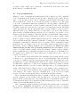
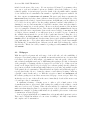
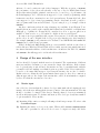
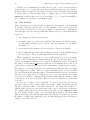
RAL-TR-2005-014
Experiences of sparse direct symmetric
solvers
J A Scott
Y Hu
September 29, 2005
Council for the Central Laboratory of the Research Councils
c Council for the Central Laboratory of the Research Councils
Enquires about copyright, reproduction and requests for additional copies of this report should
be addressed to:
Library and Information Services
CCLRC Rutherford Appleton Laboratory
Chilton Didcot
Oxfordshire OX11 0QX
UK
Tel: +44 (0)1235 445384
Fax: +44(0)1235 446403
Email: [email protected]
CCLRC reports are available online at:
http://www.clrc.ac.uk/Activity/ACTIVITY=Publications;SECTION=225;
ISSN 1358-6254
Neither the Council nor the Laboratory accept any responsibility for loss or damage arising
from the use of information contained in any of their reports or in any communication about
their tests or investigations.
RAL-TR-2005-014
Experiences of sparse direct symmetric solvers
Jennifer A. Scott1,2,3 and Yifan Hu4
ABSTRACT
We have recently carried out an extensive comparison of the performance of state-ofthe-art sparse direct solvers for the numerical solution of symmetric linear systems of
equations. In doing so, we had to familiarise ourselves with each of the solvers and to
write drivers for them. Our experiences of using the different packages to solve a wide
range of problems arising from real applications were mixed. In this paper, we highlight
some of these experiences with the aim of providing advice to both software developers
and users of sparse direct solvers. We conclude that while performance is an essential
factor to consider when choosing a code, there are other factors that a user should also
consider that vary significantly between packages.
1
Computational Science and Engineering Department, Rutherford Appleton Laboratory,
Chilton, Oxfordshire, OX11 0QX, England, UK.
Email: [email protected]
2
Current reports available from “http://www.numerical.rl.ac.uk/reports/reports.shtml”.
3
This work was supported by EPSRC grants GR/R46641 and GR/S42170.
4
Wolfram Research, Inc., 100 Trade Center Drive, Champaign, IL61820, USA.
Email: [email protected]
Computational Science and Engineering Department
Atlas Centre
Rutherford Appleton Laboratory
Oxfordshire OX11 0QX
September 29, 2005.
Scott and Hu - RAL-TR-2005-014
1
1
Introduction
For more than three decades, there has been considerable interest in the development of
numerical algorithms and their efficient implementation for the solution of large sparse
linear systems of equations Ax = b. The algorithms may be grouped into two broad
categories: direct methods and iterative methods (in recent years, hybrid methods that
seek to combine direct and iterative methods have also been proposed). The most
widely used direct methods are variants of Gaussian elimination and involve the explicit
factorization of the system matrix A (or, more usually, a permutation of A) into a product
of lower and upper triangular matrices L and U . In the symmetric case, U = DL T , where
D is a block diagonal matrix with 1 × 1 and 2 × 2 blocks. Forward elimination followed
by backward substitution completes the solution process for each given right-hand side b.
The main advantages of direct methods are their generality and robustness. For some
“tough” linear systems that arise in a number of application areas they are currently the
only feasible methods. For other problems, finding and computing a good preconditioner
for use with an iterative method can be computationally more expensive than using a direct
method. However, a significant weakness is that the matrix factors are often significantly
denser than the original matrix and, for large problems such as those that arise from
discretisations of three-dimensional partial differential equations, insufficient memory for
both forming and then storing the factors can prevent the use of direct methods. As
the size of the problems users want to solve has increased so too has interest in iterative
methods. But, because of the lack of robustness and suitability of iterative methods as
general-purposes solvers, considerable effort has also gone into developing more efficient
implementations of direct methods. During the last decade many new algorithms and a
number of new software packages that implement direct methods have been developed.
In many of our own applications we need to solve symmetric systems; the potentially
bewildering choice of suitable solvers led us to carry out a detailed study of serial sparse
direct symmetric solvers. The largest and most varied collection of sparse direct serial
solvers is that contained within the mathematical software library HSL (HSL, 2004). In
an initial study, Gould and Scott (2003, 2004) compared the performance of the symmetric
HSL solvers on a significant set of large test examples taken from a wide range of different
application areas. This was subsequently extended to all symmetric direct solvers that
were available to us. These solvers are listed in Table 1.1. Further details of the packages
together with references are given in Gould, Hu and Scott (2005b). Although a number of
the packages have parallel versions (and may even have been written primarily as parallel
codes), we considered only serial codes and serial versions of parallel solvers.
Our study was based on running each of the solvers on a test set of
88 positive-definite problems and 61 numerically indefinite problems of order at
least 10, 000.
A full list of the problems together with a brief description of
each is given in Gould, Hu and Scott (2005a).
They are all available from
ftp://ftp.numerical.rl.ac.uk/pub/matrices/symmetric. Performance profiles (see Dolan
and Moré, 2002) were used to evaluate and compare the performance of the solvers on the
test set. The statistics used were:
2
Experiences of sparse direct symmetric solvers
Code
Authors/contact
BCSLIB-EXT
The Boeing Company
www.boeing.com/phantom/bcslib-ext/
HSL codes:
MA27∗ , MA47∗, MA55∗,
MA57∗ , MA62∗, MA67∗
I.S. Duff, J.K. Reid, J.A. Scott
www.cse.clrc.ac.uk/nag/hsl and
www.hyprotech.com/hsl/hslnav/default.htm
MUMPS∗
P.R. Amestoy, I.S. Duff, J.-Y. L’Excellent, J. Koster,
A. Guermouche and S. Parlet
www.enseeiht.fr/lima/apo/MUMPS/
Oblio∗
F. Dobrian and A. Pothen
[email protected] or [email protected]
PARDISO
O. Schenk and K. Gärtner
www.computational.unibas.ch/cs/scicomp/software/pardiso
SPOOLES∗
C. Ashcraft and R. Grimes
www.netlib.org/linalg/spooles/spooles.2.2.html
SPRSBLKLLT∗
E.G. Ng and B.W. Peyton
[email protected]
TAUCS∗
S. Toledo
www.cs.tau.ac.il/∼stoledo/taucs/
UMFPACK∗
T. Davis
www.cise.ufl.edu/research/sparse/umfpack/
WSMP
A. Gupta and M. Joshi, IBM
www-users.cs.umn.edu/∼agupta/wsmp.html and
www.alphaworks.ibm.com/tech/wsmp
Table 1.1: Packages tested in our study of sparse symmetric solvers. ∗ indicates source
code is supplied.
Scott and Hu - RAL-TR-2005-014
3
• The CPU times required to perform the different phases of the direct method.
• The number of nonzero entries in the computed matrix factor.
• The total memory used by the solver.
Full details of our findings in terms of these statistics are given in Gould et al. (2005a,
2005b).
Testing the solvers involved reading the documentation, writing drivers for them and,
to ensure we were being fair and using the codes correctly, liaising with the software
developers. Our experiences were mixed. Some solvers were well documented and tested,
and their use clearly explained, and we were able to install and run them without serious
difficulties. Other software developers had paid less attention to the whole design and
testing processes so that their codes were harder to use. Some of the codes are still being
actively developed; indeed, since we embarked on our study, a number of the codes have
been significantly improved, partly as a result of feedback from us. The main aim of this
report is to highlight some of our experiences in a way that we hope will be helpful in
the future to both software developers and users of sparse direct solvers. We consider
a number of key aspects of the development of sparse solvers including documentation,
the design of the user interface, and the flexibility and ease of use. We do not try to
discuss each of the packages we tested with respect to each of these areas but we use our
experiences to illustrate the discussion. We recognise that many of our comments may be
subjective but our aim is to be as objective as possible and to base our comments on our
experiences both as software developers and as software users.
For further details of sparse direct methods, we recommend the books by Duff, Erisman
and Reid (1986) and Dongarra, Duff, Sorensen and van der Vorst (1998), and the references
therein.
We end this introductory section by explaining how to obtain the packages listed in
Table 1.1. Currently, Oblio and SPRSBLKLLT are only available by contacting the authors
directly. Some of the other packages can be downloaded straight from the webpage given.
This is the case for SPOOLES, TAUCS, UMFPACK, and WSMP (90-day evaluation license only).
A potential user of MUMPS needs to complete a short form on the webpage; the software is
then sent via email. To use PARDISO, a slightly more detailed online form must be filled in
before a license is issued and access given to download the compiled code. MA27 and MA47
are part of the HSL Archive and as such, are freely available to all for non-commercial use.
Access is via a short-lived user name and password that are sent on completing a short
form online. The remaining HSL codes require the user to obtain a licence. The software
distributors must be contacted for this. Use of BCSLIB-EXT requires a commercial licence;
contact details are on the given webpage. With the exception of BCSLIB-EXT, PARDISO,
and WSMP, source code is provided.
2
Documentation
A potential user’s first in-depth contact with the software is likely to be through the
accompanying documentation. Today this includes webpages. To be attractive to readers,
it is essential that the documentation is clear, concise and well-written. Otherwise, only
the most enthusiastic or determined user is likely to go on and use the software. There
4
Experiences of sparse direct symmetric solvers
is clearly no single “right” way to present the documentation but the aims of the writer
should always be essentially the same.
2.1
User documentation
Writing good user documentation is an integral part of the design process. The complexity
of the documentation will, in part, depend upon the complexity of the package and the
range of options that it offers. The documentation should always start with a brief
and clear statement of what, in broad terms, the package is designed to do. The main
body of the documentation must then explain how to use the package. This should be
straightforward to understand, avoiding technical terms and details of the underlying
algorithm because the reader may not be an expert on solving sparse systems. The input
required from the user and the output that will be generated must be clearly described,
with full details of any changes that the code may make to the user’s data. Readers
will not want to plough through pages and pages before being able to try out the code for
themselves, at least on a simple problem. It is generally very helpful if the calling sequence
for the package is illustrated through the inclusion of at least one simple example, which
should be supplied complete with the input data and expected output. In our experience,
if it is well-written and fully commented, this kind of example provides a template that
is invaluable, particularly for first-time users of a package. HSL documentation always
includes at least one example of how to use the package. Other packages that we tested
that include complete examples within the user documentation are BCSEXT-LIB, MUMPS,
PARDISO, UMFPACK and WSMP. Although SPOOLES, SPRSBLKLLT, Oblio and TAUCS do provide
source code for undocumented sample drivers, the advantage of having complete examples
included within the user documentation is that it forces the author to really think about
the example and to make it not only useful but also as simple and as easy to follow as
possible for new users.
For more advanced users, full details of the capabilities of the package and the options
it offers need to be given; this may involve the use of technical language. References should
be provided to available research reports and papers that describe the package and/or the
algorithm used, together with numerical results. In our opinion, all sparse direct solvers
are sufficiently complicated to require an accompanying technical report that documents
the algorithms that have been used together with important or novel implementation
details. This should enable advanced users to select suitable control parameters (see
Section 5 below) and to understand the ways in which the current package differs from
other packages. For software developers, explaining their code in a report is a useful
exercise; a careful review frequently leads to modifications and improvements.
The documentation should include details of copyright, conditions of use, and licensing.
It is also helpful to provide details of who the authors are, the date the software was
written, and the version number(s) of the package that the documentation relates to. The
documentation should provide potential users with clear instructions on how to install the
software. We discuss this further in Section 7.
The documentation supplied with the solvers included in our study varied considerably.
At one extreme, SPRSBLKLLT was supplied to us by the authors as source code and the
only items of documentation were a short ‘readme’ file, a sample driver and the comments
Scott and Hu - RAL-TR-2005-014
5
included at the start of the source. For an experienced Fortran 77 programmer, these
were easy to read and, as limited options are available, allowed the package to be used
relatively quickly. A research paper provides details of the algorithm. Oblio currently
does not include user documentation but a number of published papers are available. At
the other extreme are BCSLIB-EXT and SPOOLES. The user’s guide that accompanies the
BCSLIB-EXT library is a hefty volume, with more than 150 pages describing the use of the
subprograms for the solution of sparse linear systems. As significant portions of this need
to be read before it is possible to use the package with any confidence, this is likely to be
daunting for a novice and means that a considerable amount of time and effort must be
invested in learning how to use the package. However, as already mentioned, the inclusion
of a set of examples to illustrate the use of the software is helpful. SPOOLES has the longest
and probably the most comprehensive (but not the most readable) documentation, with
a complete reference manual of over 400 pages (a more accessible 58 page document is
also available that is intended to provide a more gentle introduction to using the code).
Some packages, including PARDISO, come with a useful reference or summary sheet, while
UMFPACK offers both a helpful and clear short introductory guide (which is sufficient to get
going with using the code) together with a much longer 133 page detailed user manual.
Subdividing the documentation into different sections with clear headings also enables
easy reference. This is done well by a number of packages, notably MUMPS, the HSL codes,
and UMFPACK.
2.2
Webpages
With the rapid development and wide usage of the world wide web, the availability of
webpages for a software package is potentially an extremely useful resource for users while
for software developers it offers unique opportunities to raise the profile of their codes
and a relatively straightforward way of distributing their packages globally. A discussion
of the principles of designing effective webpages is beyond the scope of this report but
clearly a well designed and developed webpage for a software package should contain (or
give pointers to) all the details and information that were previously only available as part
of the printed user documentation. This will include user guides and additional papers or
reports, plus details of how to obtain the software, version history, licensing conditions,
copyright, contact details, and so on. With the exception of Oblio and SPRSBLKLLT, all
the software packages we tested have an associated webpage of some sort (see Table 1.1).
As already noted, some of these allow the user to immediately download the most recent
code and up-to-date documentation.
A significant advantage of having access to either a pdf or html version of the
documentation that we appreciated while testing the packages is the ability to search
with ease for a key word or phrase. Where the user interface is complicated, this can be
much easier that using the printed or postscript version of the documentation. MUMPS and
UMFPACK are examples of packages that include freely available pdf versions of their user
documentation on their webpages.
Some webpages, including those for MUMPS, have a ‘frequently asked questions’ section.
These can be helpful but must not be an excuse for failing to offer fully comprehensive
and complete user documentation.
6
Experiences of sparse direct symmetric solvers
3
Language
In Table 3.2 we list the languages that the solvers are written in. Many authors choose a
particular language because they are familiar with it and it is what they always use. HSL,
for example, has always been a Fortran library so its packages are written in Fortran 77
or, more recently, Fortran 90 or 95. Others may choose a language because they would
like to take advantage of some of the features that it offers but that are not available in
another language. For example, a developer may want to exploit the high level of support
for object oriented programming offered within C++ or may wish to avoid Fortran 77
because of its lack of dynamic memory allocation. However, since the solvers are intended
for others to use, it is always important before choosing the language to consider what is
likely to be most convenient for potential users.
Code
Language
64-bit
Comments
BCSLIB-EXT
Fortran 77
MA27
Fortran 77
MA47
MA55
MA57
MA62, MA67
Fortran
Fortran
Fortran
Fortran
MUMPS
Fortran 90
C interface available
Oblio
C++
Object-oriented code
PARDISO
Fortran 77 & C
SPOOLES
C
SPRSBLKLLT
Fortran 77
TAUCS
C
UMFPACK
C
WSMP
Fortran 90 & C
Fortran 90 interface available within the GALAHAD
optimization package as routine SILS
(see galahad.rl.ac.uk/galahad-www)
77
90
77/Fortran 90
77
Fortran 77 and Fortran 90 versions available
√
Both languages are used in the source code
Object-oriented code
√
An early version (MA38) was written in Fortran 77.
Object-oriented code.
Fortran 77 and MATLAB interfaces.
Both languages are used in the source code
Can be called from Fortran and C programmes
Table 3.2: Languages the solvers are written in.
Our benchmarking experience suggested that, for direct solvers, there is little to choose
between the three popular languages, Fortran, C and C++ in terms of performance –
Scott and Hu - RAL-TR-2005-014
7
efficient code can be written in each of these languages. With the exception of SPOOLES,
the performance of the solvers relies heavily on the use of Level 3 BLAS (Basic Linear
Alegra Subroutines); highly optimised versions need to be used for good performance. Of
the main languages, C++ offers the most support for object oriented programming, which
is attractive as well as convenient for some developers and users. Fortran 90/95 also offers
some support for object oriented programming. On the other hand, it is also possible to
write programs with clean and well defined “objects” using C; a good example of this is
UMFPACK.
Another consideration when choosing a language is portability. C and Fortran 77 are
arguably the most portable, with compilers almost always freely available on all platforms.
Although good quality free Fortran 90/95 compilers were slow to appear, g95 is now
available so that access to a good Fortran 95 compiler is also now widespread.
Because a user’s program that calls a sparse solver may not be in the same language
as the solver, it can be helpful if the developer provides interfaces in other languages.
For example, UMFPACK provides interfaces for Fortran 77 and MATLAB while MUMPS and
PARDISO can be called from C programs.
With both Intel and AMD having 64-bit processors available, and the recent release of
64-bit editions of Windows XP and Windows Server 2003, users are increasingly interested
in software that makes full use of 64-bit architecture. As indicated in Table 3.2, PARDISO
and UMFPACK offer full support for 32-bit and 64-bit architectures.
4
Design of the user interface
A solver should be designed with the user’s needs in mind. The requirements of different
users vary and they determine, to some extent, the design of the interface. If the software
is to be general purpose and well used, the interface needs to be straightforward, with the
potential for the user making errors limited as far as possible. If the solver is intended to
be used to solve many different types of problems, the interface also needs to be flexible.
In this section, we discuss how the sparse matrix data is passed to the solver, comment on
different approaches to the design of the user interface, and look at information computed
by the solver that the user may need access to.
4.1
Matrix input
One of the key decisions that the software developer must make when designing the user
interface is how the user will supply the (nonzero) entries of the system matrix A. The aim
should be for this to be simple for the user (so that the chances of errors are minimised)
as well as efficient in terms of both time and memory. The developer clearly has a number
of options available. These include:
(a) Inputting all the entries on a single call using real and integer arrays. We refer to this
as standard input.
(b) Inputting the entries of A one row at a time. This is called reverse communication
and can be generalized to allow a block of rows to be input on a single call. In the
8
Experiences of sparse direct symmetric solvers
case of element problems where A is held as a sum of small dense element matrices,
the elements are input one at a time.
(c) Requiring the user to put the matrix data into one or more files that can be read by
the software package as they are required.
There can be advantages in making the interface flexible by offering a choice of input
methods because the form in which the matrix data arises depends very much on the
application and origins of the problem. For the user, a potential downside to having a
choice is, of course, more complicated and lengthy documentation and possibly a greater
chance of making input errors. For the software developer, more options means more code
to maintain and to test, again with a greater potential for errors. The only package in
our survey of symmetric solvers that offers more than one of the above input methods is
BCSLIB-EXT (it offers (a) and (b)), while TAUCS is the only solver that uses files to input
the matrix. The latter offers a number of different formats, including coordinate and
compressed sparse column formats. Alternatively, a user may access the TAUCS matrix
structure to input the matrix.
A small number of codes in our study have reverse communication interfaces, namely,
the band solver MA55, the frontal code MA62 (both from the HSL library), and BCSLIB-EXT.
The main advantage of reverse communication is that, at each stage, the user only needs
to generate and hold in main memory a small part of the system matrix. This may be
important, for example, for large-scale three-dimensional finite-element applications for
which the additional memory required if all the elements are generated and stored in
memory prior to using the package may be prohibitive.
The HSL code MA55 requires the lower triangular part of the matrix to be entered
a block of rows at a time. The user can choose to specify the rows one at a time, but
the documentation notes that specifying more than one at once reduces procedure call
overheads and the overheads of several statements that are executed once for each call.
MA62 is for finite-element problems only and requires the user to enter the upper triangular
parts of the element matrices one at a time. BCSLIB-EXT has a number of different reverse
communication options. The matrix can be entered a single entry at a time, by adding
a vector of entries on each call, or by entering the element matrices one by one. A key
difference between the two HSL codes and BCSLIB-EXT is that the former have reverse
communication interfaces for both the analyse and factorize phases, whereas for the latter
the user enters the whole of A using a series of calls prior to the analyse phase and the
package then accumulates the system matrix and optionally holds it out-of-core.
Many users initially find reverse communication harder to use than supplying the
matrix data in a single call because the documentation tends to be longer and more
complicated. Moreover, there is an overhead for making repeated calls to the input routine.
Thus it can be advantageous to include standard input as an option along with reverse
communication.
If standard input is used, the software designer still has a number of options.
(i) Coordinate format (COORD), that is, for each nonzero entry in A, the row index i,
the column index j, and the value aij are entered. This requires two integer arrays
and one real array of length nz, where nz is the number of nonzero entries in A.
9
Scott and Hu - RAL-TR-2005-014
(ii) Compressed sparse column format (CSC). In this case, the entries of column 1 must
proceed those in column 2, and so on. This requires an integer array and a real
array of length nz plus an integer array of length n + 1 that holds ‘pointers’ to the
first entry in each column. In some cases, the package requires that the entries in a
given column must be supplied in ascending order. This extra manipulation by the
user may make the job of the software writer easier (and may lead to some savings
in the computational time and memory requirements), but it can deter users what
are unfamiliar with working with large sparse matrices.
(iii) For element applications where A is held as a sum of small dense matrices, element
format (ELMNT) can be used. In this case, the entries for the dense matrix
corresponding to element 1 proceed those corresponding to element 2, and so on.
This requires an integer array to hold the lists of integers in each of the elements
and an integer array of length nelt + 1 that holds ‘pointers’ to the position of the
start of the integer list for each element. A real array must hold the corresponding
element entries.
For symmetric matrices, with the exception of SPRSBLKLLT, the solvers require only
the entries in the upper (or lower) triangular part of A (in the element case, only the
upper triangular part of each element is needed). Coordinate format is perhaps the
simplest input format for inexperienced users, especially those who are not familiar
with sparse matrix data formats. The disadvantage of COORD compared with CSC
is the need for two integer arrays of length nz, instead of one. Because of the savings
in storage, matrices in sparse test sets such as the Harwell-Boeing Sparse Matrix
Collection (www.cse.clrc.ac.uk/nag/hb/hb.shtml) and the University of Florida Sparse
Matrix Collection (www.cise.ufl.edu/research/sparse/matrices/) are stored in CSC format.
Thus a software developer who offers CSC input will find it straightforward to test his or
her package on these test problems.
Code
BCSLIB-EXT
MA27
MA47
MA57
MA67
MUMPS
Oblio†
PARDISO†
SPOOLES†
SPRSBLKLLT
UMFPACK
WSMP†
COORD
√
√
√
√
√
√
Format
CSC ELMNT
√
√
√
√∗
√
√
√∗
√
Table 4.1: The input format offered by the codes in our study that use standard input. ∗
indicates the entries in each column must be in ascending order and † indicates that the
diagonal must be entered explicitly.
10
Experiences of sparse direct symmetric solvers
In Table 4.1, we summarize the formats offered by the codes in our study that use
standard input. A ∗ for the CSC entry indicates that the entries in each column of
the matrix must be supplied in ascending order and † indicates that the diagonal must
be present (any zero diagonal entries must be explicitly entered). We note that while
UMFPACK has a CSC interface it also provides a utility code to convert from COORD to
CSC; a similar code is available on the WSMP webpage.
4.2
User interface
Sparse direct methods solve systems of linear equations by factorizing the coefficient matrix
A, generally employing graph models to try and minimize both the storage needed and
work performed. Sparse direct solvers have a number of distinct phases. Although the
exact subdivision depends on the algorithm and software being used, a common subdivision
is given by:
1. An ordering phase that exploits structure.
2. An analyse phase (or symbolic factorization) that analyses the matrix structure
to (optionally) determine a pivot sequence and data structures for an efficient
factorization.
3. A factorization phase that uses the pivot sequence to factorize the matrix.
4. A solve phase that performs forward elimination followed by back substitution using
the stored factors. The solve phase may include iterative refinement.
When designing the user interface for each of these phases, it is good programming
practice to hide details that are implementation specific from the user, using object
oriented programming techniques. For example, in UMFPACK the call to its symbolic
factorization routine umfpack symbolic returns an object symbolic in the form of a C
pointer, instead of using arrays to hold details of the matrix ordering and pivot sequence.
The symbolic object must be passed to the numerical factorization routine, and finally
deleted using another routine. This sort of approach (which can also be achieved within
C++ and Fortran 90/95) limits the number of arguments that the user has to understand
and pass between subroutines, reducing the scope for errors and allowing the software
developer the possibility of changing internal details in future without causing problems
for the user’s code. For more experienced users, a means of accessing these objects should
be provided.
Another way of trying to reduce the likelihood of a user introducing errors between
subroutine calls is to have a single callable user routine. MUMPS adopts this approach
and uses a parameter JOB to control the main action. By setting this parameter to
different values, the user can call a single phase of the solver or can execute several phases
(for example, analyse then factorise and then solve) with one call. PARDISO and WSMP
also have a single callable routine. Some users find this is simpler to use than calling
different subroutines with different arguments for the various solver phases but, provided
the number of callable subroutines is modest, choosing which approach is best is largely
a matter of personal preference.
Scott and Hu - RAL-TR-2005-014
11
The HSL routines, in general, have four main user-callable subroutines: an initialisation
routine that set defaults for the control parameters (see Section 5.5), one for the analyse
phase (incorporating the ordering), and one each for the factorization and solve phases.
MA57 offers additional routines, for example, for performing iterative refinement, while
MA62 has a routine the user must call before the factorization if out-of-core working is
wanted.
BCSLIB-EXT has many subroutines the user can call (including initialisation routines,
a number of routines for entering the matrix sparsity pattern and numerical entries,
reordering, performing the symbolic factorization, the numerical factorization, and the
forward and back substitutions). They are all fully documented but, as already noted,
with so many subroutines to understand and to call, our experience was that a lot of effort
had to be invested before it was possible to start using the package. The TAUCS package
also contains a large number of routines because the package has been designed so that the
user must call different routines if, for example, the out-of-core version is required. While
having separate routines may simplify development and testing for the developer, it can
make the user’s job more complicated if experiments with both out-of-core and in-core
codes are required.
UMFPACK is another example of a package with many routines; it has 32 user callable
routines. Of these, five are so-called primary routines, which are documented in the quick
start user guide and are all a beginner needs to get going with the package. The other
27 routines are available to provide additional facilities for more experienced users. They
include matrix manipulation routines, printing routines and routines for obtaining the
contents of arrays not otherwise available to the user. The simplest interface of all and
an example of a single call routine is the MATLAB interface to UMFPACK (Version 4.3 is a
built-in routine for lu, backslash, and forward slash in MATLAB 7.1).
4.3
Information returned to the user
A well designed solver will provide the user with information, both on successful completion
and in the event of an error (see Section 6). After the symbolic factorization, information
should be returned to the user on the estimated number of entries in the factor, the
estimated flop count, and the estimated integer and real memory that will be required for
the factorization. These estimates should help the user to decide whether or not to try
and proceed with the factorization and, for solvers in Fortran 77, give the user an idea of
how to appropriately allocate workarrays and arrays for holding the factors.
Once the factorization is complete, the user should have details of the number of entries
in the factors, the flop count, and the amount of real and integer memory used. For those
wishing to solve a series of problems, it can also be useful to provide information on the
minimum memory that would be required if the factorization were to be repeated.
Other information that is provided by one or more of the solvers we tested and that
we think is useful includes the number of matrix entries that were ignored (because they
were out-of-range), the number that were duplicates, the determinant of the matrix, the
computed inertia, the norm of the matrix and its condition number, information on the
pivots used (such as the number of 2 × 2 pivots), and the number of steps of iterative
refinement that have been performed. For frontal and multifrontal codes it is also useful
12
Experiences of sparse direct symmetric solvers
to know the maximum frontsize and, more generally, for multifrontal codes, details of
the elimination tree (such as the number of nodes in the tree). Clearly, some of this
information will only be of interest to experts.
Many solvers use “information arrays” to return information to the user. Some have
a single array, others use two (one for real and the other for integer information). These
arrays are output arrays only, that is, they are not set by the user. Solvers using these
arrays include the HSL codes, MUMPS and UMFPACK (the latter provides a routine for printing
the information array). We found PARDISO and WSMP less convenient since their array
IPARM contains a mix of input and output parameters; some of the components must be
set on entry and others are only set on exit. In Fortran 90/95 derived types can be used,
which can be more user-friendly as it allows meaningful names to be used in place of
entries in an array. However, printing a simple list of the information generated is then
less straightforward, and we would recommend providing a separate printing routine to
do this.
5
Flexibility and the use of parameters
Each of the sparse solvers used in our numerical experiments offers the user a number of
options. These provide flexibility and, to some extent, allow the user to choose algorithms
and control the action. In this section we discuss some of these options.
5.1
Ordering choices
One of the keys to the success of any sparse direct solver is the ordering algorithms
that it offers. There are a number of different approaches to the problem of obtaining a
good pivot sequence and no single method is universally the best. As a result, a good
solver should have access to a choice of orderings. To ensure minimum in-core storage
requirements, ordering algorithms are not integrated within the out-of-core HSL codes
MA55 and MA62 that have a reverse communication interface. The user must preorder
the rows or elements; additional routines are provided within HSL that can be used for
this. For the other solvers in our study, the ordering options are summarized in Table 5.1.
An entry marked with ∗ indicates the default ordering (where more than one entry for a
solver is marked with an ∗ it is because the solver automatically chooses which ordering
to use based on the input matrix). In addition, with the exception of MA67, the user
may supply his or her own ordering. However, to do this for SPRSBLKLLT or UMFPACK,
the user must preorder the matrix before entry to the solver; the other packages perform
any necessary permutations on the input matrix using the supplied ordering. MA67 is
somewhat different in that it is an analyse-factorize code, that is, it combines the symbolic
and numerical factorization phases. Test results have shown that this can work well on
highly ill-conditioned indefinite problems but it is unsuitable in the situation where a user
wants to solve a sequence of sparse linear systems where the coefficient matrices change but
their sparsity pattern remains fixed. A key advantage of designing a solver with separate
analyse and factorize phases is that the work of choosing a pivot sequence does not have
to be repeated. Furthermore, when many problems of a similar type need to be solved, it
may be worthwhile to invest time in trying out different pivoting strategies.
13
Scott and Hu - RAL-TR-2005-014
Code
BCSLIB-EXT
MD
×
AMD
×
MMD
√
ND
×
METIS
√∗
MS
×
MF
×
MK
×
MA27
√∗
×
×
×
×
×
×
×
MA47
×
×
×
×
×
×
×
MA57
√
√∗
×
×
×
×
MA67
×
×
×
×
×
×
×
MUMPS
√
√∗
×
×
√∗
√
√
Oblio
×
×
×
×
×
PARDISO
×
×
×
×
×
SPOOLES
×
×
×
×
SPRSBLKLLT
×
×
×
×
×
TAUCS
√
√
×
×
×
UMFPACK
×
×
×
×
×
WSMP
×
×
×
√∗
×
√
√
√
√∗
√
×
×
×
×
√∗
×
×
×
√∗
√∗
√∗
√∗
×
×
√∗
√∗
√∗
√∗
×
√∗
×
×
Table 5.1: Ordering options for the solvers in our study. MD = minimum degree; AMD =
approximate minimum degree, MMD = multiple minimum degree; ND = nested dissection;
METIS = explicit interface to METIS NodeND (or variant of it); MS = multisection; MF =
minimum fill; MK = Markowitz). ∗ indicates the default.
14
5.2
Experiences of sparse direct symmetric solvers
Factorization algorithms
Following the selection of the pivot sequence and the symbolic factorization, the numerical
factorization can be performed in many different ways, depending on the order in
which matrix entries are accessed and/or updated. Possible variants include left-looking,
right-looking, frontal, and multifrontal algorithms. Most solver packages offer just one
algorithm. The software developer will have his or her own reasons for choosing which
method to implement (based on their own experiences, ease of coding, research interests,
applications, and so on). In our tests on large problems that were taken from a range of
applications, we did not find one method to be consistently better than the others. Oblio
is still being actively developed as experimental tool with the goal of creating a “laboratory
for quickly prototyping new algorithmic innovations, and to provide efficient software on
serial and parallel platforms”. Its object-orientated design includes implementations of
left-looking, right-looking, and multifrontal algorithms. For 2-dimensional problems the
authors recommend the multifrontal option but for large 3-dimensional problems the user
documentation reports the multifrontal factorization can be outperformed by the other
two algorithms. TAUCS, which is also still under development, is designed to provide a
library of fundamental algorithms and services, and to facilitate the maintenance and
distribution of the resulting research codes. It includes both a multifrontal algorithm and
a left-looking algorithm.
5.3
Out-of-core options
Even with good orderings, to solve very large problems using a serial direct solver it is
usually necessary to work out-of-core. By holding the matrix and/or its factor in files,
the amount of main memory required by the solver can be substantially reduced. Only a
small number of direct solvers currently available include options for working out-of-core.
BCSLIB-EXT, MA55, MA62, Oblio, and TAUCS allow the matrix factor to be held out-of-core.
Oblio also allows the stack used in the multifrontal algorithm to be held in a file. As
already noted, BCSLIB-EXT, MA55 and MA62 have reverse communication interfaces and
so do not require the matrix data to be held in main memory, reducing main memory
requirements further. The most flexible package is BCSLIB-EXT. It offers the option of
holding the matrix data and/or the stack in direct access files and, if a front is too large
to reside in memory, it is temporarily held in a direct access file. In addition, information
from the ordering and analyse phases may be held in sequential access files.
In the future, as the size of problems that users want to be able to solve continues to
grow, the need for solvers that offer out-of-core facilities is also likely to grow. Of course,
there are penalties for out-of-core working. The software is necessarily more complex
and the I/O overheads lead to slower factorize and solve times (for a single or small
number of right-hand sides, the I/O overhead for the solve phase is particularly significant).
Important challenges for the software developer are minimising the additional costs and
ensuring that the user interface does not become over-complicated because of the out-ofcore working.
Scott and Hu - RAL-TR-2005-014
5.4
15
Multiple right-hand sides
An important advantage of direct methods over iterative methods is that, once the factors
have been computed, they can be used to solve repeatedly for different right-hand sides.
They can also be used to solve for more than one right-hand side at once. In this case, the
software can be written to exploit Level 3 BLAS in the solve phase. If Level 3 BLAS is
used, solving for k right-hand sides simultaneously is significantly faster than solving for a
single right-hand side k times. Most modern direct solvers allow the solution of multiple
right-hand sides.
5.5
Control parameters
As the name suggests, control parameters are parameters that may be selected by the user
to control the action. Some solvers offer the user a large degree of control (for example,
BCSEXT-LIB, MA57 and UMFPACK), while others (including SPRSBLKLLT) leave few decisions
open to the user. Clearly, a balance has to be achieved between flexibility and simplicity
and this will, in part, depend on the target user groups.
Although the user can set the control parameters, defaults (or at least, recommended)
values need to be chosen by the software developer. These are selected on the basis of
numerical experimentation as being in some way the “best all round” values. Getting these
choices right is really important because, in our experience, many users (in particular,
those who would regard themselves as non-experts) frequently rely on the default settings
and are reluctant to try other values (possibly because they do not feel confident about
making other choices). Thus the developer needs to experiment with as wide a range of
problems as possible (different problem sizes and, for a general purpose code, different
application areas and different computing platforms). There will inevitably be situations
when the defaults may give far from optimal results and the user will then need to try
out other values. The ability to try different values can also be invaluable to those doing
research. The developer may need to change the default settings at a later date as a result
of hardware developments.
In addition to controlling the ordering performed and the factorization algorithm used,
the most often used control parameters control the following actions:
Threshold pivoting (solvers that are designed to handle both positive and indefinite
problems). Pivoting for stability involves using a threshold parameter to determine
whether a pivot candidate is suitable. Small values favour speed and sparsity of the
factors but at the potential cost of instability. The default value for the threshold
is not the same for all solvers but is usually 0.1 or 0.01. It is important to be able
to control this parameter since in some optimization applications, for example, very
small values are used to ensure speed (and iterative refinement is relied upon to
recover accuracy). If pivoting is not required (because the user knows the problem is
positive definite), setting the threshold to 0 normally means no pivoting is performed
and a logically simpler path through the code is followed (which should reduce the
execution time).
Pivoting strategy This is currently an active area of research and recent versions of
some of the solvers are now offering a number of pivoting strategies. This is discussed
16
Experiences of sparse direct symmetric solvers
further in Section 6.3. A number of codes (including the HSL codes) allow the user
to specify the minimum acceptable pivot size. If perturbations of pivots that are
unacceptably small is offered, some solvers (for instance, PARDISO) give the user
control over the the size of the perturbations.
Iterative refinement It is helpful to offer the user facilities for automatically performing
iterative refinement and for computing the norm of the (scaled) residual. A number
of solvers, including MA57, MUMPS, Oblio, PARDSIO, UMFPACK and WSMP, do offer this.
A control parameter is used to specify the maximum number of steps of iterative
refinement. In addition, MUMPS has a parameter that allows the user to specify
the required accuracy while MA57 has a parameter for monitoring the speed of
the convergence of iterative refinement: if convergence is unacceptably slow, the
refinement process is terminated. WSMP allows the user to request that iterative
refinement be performed in quadruple precision.
Scaling Poorly scaled problems can benefit from being scaling prior to the numerical
factorization. MA57, MUMPS, UMFPACK and WSMP offer scaling as an option (there are
also separate HSL codes that can also be used to prescale a problem).
Condition number estimation This involves additional work but is useful as a measure
of the reliability of the computed solution. It is currently offered by a few solvers,
including MA57 and WSMP.
Diagnostic printing The user needs to be able to control the unit number on which
printing is performed as well as the amount of diagnostic printing. When a solver
is incorporated within another package, it is important to be able to suppress all
printing, while for debugging purposes, it can be useful to be able to print all
information on input and output parameters. Thus it is common practice to offer
different levels of printing and allow the user to choose different output streams for
errors, for warnings, for diagnostic printing and the printing of statistics. Examples
of packages with a range of printing options are MA57 and MUMPS. UMFPACK uses a
different approach: its main routines perform no printing but nine separate routines
are available that can be used to print input and output parameters.
Blocking As already noted, modern direct solvers generally rely on extensive use of high
level BLAS routines for efficiency. Since different block sizes are optimal on different
computer architectures, the block size should be available for the user to tune. Codes
with a block parameter include BCSLIB-EXT, MA57, MA62, MA67, and UMFPACK (the
default is not the same for each of these solvers).
A simple and, in our experience, convenient way to organize the control parameters is
to hold them using either a single array or two arrays (one for integer controls and one for
real controls), or possibly three arrays (the third array being a logical array since often a
number of the controls can only be either “on” or “off”). A number of solvers (including
BCSLIB-EXT, the HSL codes and MUMPS) provide an initialisation routine that needs to be
called to assign default values to the control arrays. If other values are wanted, the relevant
individual entries of the control arrays can be reset by the user after the initialisation and
Scott and Hu - RAL-TR-2005-014
17
prior to calling other subroutines in the package. For BCSLIB-EXT, the user has to call a
separate subroutine to reset one control parameter at a time. This can be cumbersome if
several controls need to be reset. Other solvers simply require the user to overwrite the
default and we found this easier to use. PARDISO and WSMP do not have an initialisation
routine but use the first entry in an integer array IPARM to indicate whether the user wants
to use defaults. If IPARM(1) is set to 0, defaults are used, otherwise all the control integer
parameters must be set by the user. We found that this is not very convenient if, for
example, only one control that differs from the default is wanted. If a fixed length array
is used for the controls, we recommend the software developer allows some extra space
for controls that may be wanted in the future. The software should always check that the
user-supplied controls are feasible; if one is not, we suggest a warning is raised and the
default value is used.
An alternative is to use a derived type whose components are control variables. As
mentioned earlier, this can be more user-friendly as it allows meaningful names to be
used for the controls. It is also more flexible as additional controls can be easily be added.
Another possible way of setting controls is through the use of optional arguments. UMFPACK
uses an optional array. If the user passes a NULL pointer, the default settings are used.
Finally, we note that it is important that the user documentation clearly explains
the control parameters (possibly with suitable references to the literature). However, as
they are primarily intended for tuning and experimentation by experts, they should not
complicate the documentation for the novice user. A user also needs to know the range of
values that are possible and what, in broad terms, the effect of resetting a parameter is
likely to be. If a parameter is important enough for the software developer to want the user
to really consider what value to use (which may be the case if, for instance, the best value
is too problem dependent for the writer to choose a default), then that parameter should
not be a control but should be passed to the routine as a regular argument. An example
might be the use of scaling. Our experience has been that the benefits of different scaling
strategies are highly problem dependent and so we feel a user should really be aware of
what scaling, if any, is being performed.
6
What if things go wrong?
An important consideration when developing any software package designed for use as
a ‘black box’ routine is the handling of errors. One of the main attractions of direct
methods that is often cited is their robustness. However, the software developers should
always have in mind what can go wrong and, for the solver to be both user friendly and
robust, it must be designed to ‘fail gracefully’ in the event of an error. In other words,
the package should not crash when, for example, a user-supplied parameter is out-of-range
or the available memory is insufficient; instead, it should either continue after issuing a
warning and taking appropriate corrective action or stop with an error returned to the
user. In both cases, the user needs to be given sufficient details to understand what has
gone wrong together with advice on how to avoid the error in a future run. Because sparse
solvers are often embedded in application software, such information should be returned
using error flags and there should be a way to suppress any warning and error messages.
Most of the solvers we tested fulfil this requirement.
18
Experiences of sparse direct symmetric solvers
The main potential sources of problems and errors for sparse direct solvers can be
categorised as follows:
1. The user-supplied data
2. Memory problems
3. Pivoting difficulties
4. In addition, if a code offers out-of-core working, this can potentially lead to problems.
We discuss each of these in turn.
6.1
Input data problems
One of the most likely causes of the solver failing is an error in the user-supplied data.
In Section 4, we discussed the input data. Even experienced users may make an error
setting up this data. A parameter may be out-of-range or, when using a package such
as OBLIO, PARDISO or SPOOLES that requires the sparsity pattern of the input matrix to
include the diagonal, the user may fail to explicitly supply zero diagonal entries. The
more complicated the user interface is, the more necessary it is for the package to perform
comprehensive testing of the input. Checking scalar parameters is quick and easy to do.
Checking arrays, such as the index arrays that define the sparsity pattern, is more time
consuming and the software developer needs to ensure it is done as efficiently as possible
so that it represents only a small fraction of the total run time. Efficiency of the data
checking is particularly important for smaller problems for which error checking can add
a significant overhead.
The ‘user’ of the solver may be another package that has already checked the matrix
data, in which case checking of the input data may be unnecessary. Similarly, when solving
a sequence of problems in which the numerical values of the entries of A change but the
sparsity pattern does not, checking may be redundant after the first problem. Thus, for
some users it may be useful to include an option that allows checking of the input data
to be switched off. Of course, if checking is switched off and there is an error in the user’s
data, the results will be unpredictable so we would recommend that the default be always
to perform error checking.
Some software developers have decided not to offer comprehensive checking of the user
data. For example, the documentation for WSMP states that it performs ‘minimal input
argument error-checking and it is the user’s responsibility to call WSMP subroutines with
correct arguments ... In the case of an invalid input, it is not uncommon for a routine to
hang or to crash with a segmentation fault’. At least the documentation is clear that no
responsibility is taken for checking of the user’s data; the documentation for other codes
is often less transparent. For example, PARDISO returns an error flag of -1 if the input is
‘inconsistent’ but no further details are given. This does not help the user track down the
problem. Furthermore, the PARDISO documentation does not make it clear what checking
is performed. For this code, we feel that full checking should be offered because the input
required is reasonably complicated (any zero diagonal entries must be stored explicitly
and the nonzeros within each row of A must be held in increasing order).
Scott and Hu - RAL-TR-2005-014
19
A number of packages we tested (including the HSL codes and MUMPS) allow out-ofrange and/or duplicated entries to be included. Out-of-range entries are ignored and
duplicates are typically summed, which is what is needed, for example, in finite-element
problems when the element contributions have not been summed prior to calling the
solver. The user needs to be warned if entries have either been ignored or summed since
such entries may represent an error that he or she needs to be made aware of so that the
appropriate action can be taken. A warning can be issued by setting a flag and, optionally,
printing a message. As discussed in Section 5, the printing of error and warning messages
needs to be under the user’s control.
An advantage of a reverse communication interface is that it can be designed to allow
the user to recover after an input error, that is, the user may be allowed to reenter an
element (or equation) in which an error has been encountered without reentering the
previously accepted elements (or equations).
6.2
Memory problems
The codes that do not offer out-of-core facilities will inevitably face difficulties as problem
sizes are increased. For positive definite problems, the analyse phase can accurately
predict the memory requirements for the subsequent factorization; both the size of the
matrix factor and the required workspace can be determined. Provided this information
is returned to the user, he or she can determine a priori whether sufficient memory is
available.
Solving indefinite problems is generally significantly harder since the pivot sequence
chosen during the analyse phase based on the sparsity pattern may be unstable when
used for the numerical factorization. If pivots are delayed because they do not satisfy the
threshold test, the predictions from the analyse phase may be inaccurate and significantly
more workspace as well as more storage for the factor may be required. For Fortran 77
packages, the memory must be allocated by the user and passed to the package as real
and integer arrays. If the memory is insufficient, the solver will terminate (hopefully
with some advise to the user on how far the factorization has proceeded and how much
additional memory may be needed). The Fortran 77 solver MA57 is optionally allows the
user to allocate larger work arrays and then restart the factorization from the point at
which it terminated. We found this less convenient than working with a solver that can
automatically allocate and deallocate memory as required (especially since once larger
arrays have been chosen, there is still no guarantee that they will be large enough and the
process may need to be repeated); it also complicates the documentation.
6.3
Pivoting problems and singular matrices
As already noted, for symmetric indefinite problems, using the pivot sequence chosen by
the analyse phase may be unstable or impossible because of (near) zero diagonal pivots.
A number of codes in our study (MA55, MA62, SPRSBLKLLT, and TAUCS) do not try and
deal with this and, as they state in their documentation, they are only intended for
positive definite problems; a zero pivot will cause them to stop. The default within
WSMP is also to terminate the computation as soon as a zero pivot (or one less than a
tolerance) is encountered. The code also offers an option to continue the computation by
20
Experiences of sparse direct symmetric solvers
perturbing near zero pivots. The data structures chosen by the analyse phase can be used
but large growth in the entries of the factors is possible. The hope is that accuracy can
be restored through the use of iterative refinement but, with no numerical pivoting, this
simple approach is only suitable for a restricted set of indefinite problems.
A larger set of problems may be solved by selecting only numerically stable 1×1 pivots
from the diagonal, that is, a pivot on the diagonal is only chosen if its magnitude is at least
u times the largest entry in absolute value in its column, where 0 < u ≤ 1 is the threshold
parameter (see Section 5.5). Potentially unstable pivots (those that do not satisfy the
threshold test) will be delayed, and the data structures chosen during the analyse phase
may have to be modified.
To preserve symmetry and maintain stability, pivots may be generalised to 2 × 2
blocks. Again, different packages use different 2 × 2 pivoting strategies. PARDISO only
looks for suitable pivots within the dense diagonal blocks that correspond to supernodes
and, if a zero (or nearly zero) pivot occurs, it is perturbed. Numerical stability is
not guaranteed (the hope again is that iterative refinement, which by default is always
performed by PARDISO if pivots have been perturbed, will restore the required accuracy).
The attractions of this static pivoting approach (a version of which is also offered by the
latest version of MA57) are that, because there is no searching or dynamic reordering during
the factorization, the method is fast and allows the data structures set up by the analyse
phase to be used. Thus errors resulting from of a lack of memory will not occur during
the factorization and there will be no additional fill in the factors resulting from delayed
pivots. The user should, however, be very aware of the potential pitfalls. In particular,
there is no guarantee that iterative refinement will converge to the required accuracy and,
because a perturbed system has been solved, the user cannot be provided with inertia
details for the original system. In some applications, such as constrained optimization,
this information is important. We note that PARDISO does return the computed number
of positive and negative eigenvalues but the documentation does not clearly explain that
these are for a perturbed matrix and could be very different from the exact inertia of the
input matrix.
A more stable but complicated approach for indefinite problems combining the use of
1 × 1 and 2 × 2 pivots is implemented by default within BCSLIB-EXT, MA27, MA47, MA57,
MA67, Oblio and the most recent verion of MUMPS. Each follows a slightly different strategy
but they can all potentially result in a large number of pivots being delayed, possibly
leading to solver failure because of insufficient memory (the out-of-core facilities offered
by BCSLIB-EXT mean that it does not run out of memory but the factorization time can
be unacceptably slow). This was observed during our numerical experiments for a number
of “tough” indefinite problems.
Some of the problems in our test set turned out to be singular. For a user who does
not know a priori whether or not a problem is singular, it can be useful to offer the option
of continuing the computation after singularity has been detected. A number of packages
we tested do offer this. In particular, the HSL codes that use 1 × 1 and 2 × 2 pivoting
issue a warning and continue the computation. Provided the given system of equations
is consistent, they compute a consistent solution and provide the user with the computed
rank of the matrix. An example where this may be useful is when A has one of more rows
that are completely zero (with the corresponding entries in the right-hand sides also zero).
Scott and Hu - RAL-TR-2005-014
21
UMFPACK also warns the user if the matrix is found to be singular. Its documentation states
that a valid numerical factorization has been computed but a divide by zero will occur if
the solve phase is called. Other codes, such as BCSLIB-EXT and MUMPS, terminate with an
error once singularity is detected.
6.4
Out-of-core problems
Out-of-core working has the potential to lead to errors that can be difficult for the user
to overcome. If the code chooses (as MA55 does) the unit numbers for reading and writing
files, it will fail if no available unit can be found. The code will also fail if it runs out
of disk space. So that the user can take advantage of any large amounts of disk space,
MA62 and TAUCS both allow the user to specify where the files will be written, which does
not have to be where the executable is located. Unfortunately, out-of-core solvers can still
run out of main memory. TAUCS, for example, holds the matrix factor out-of-core but the
frontal matrices are held in main memory so on large problems, the main memory can still
be insufficient.
7
Installation
It is important that software developers consider how best to advise and help users install
their software. As noted in Table 1.1, many of the packages are provided as source code.
This has the advantage that users can put the software onto whichever machines they
choose and they are in control of the compilation process, but it also means extra effort
is needed by the user, who will often not be a systems expert. It is important to make
the need for external codes (such as routines from the BLAS and LAPACK libraries, or
ordering algorithms such as METIS) very clear, without assuming the user has previous
experience of these libraries. Performance (speed) will typically be critically influenced by
the use of appropriate BLAS so the user needs to be made aware of this and instructed
on how to obtain fast BLAS for his or her computer. Links from the solver’s webpage to
sites where fast BLAS and, where necessary, LAPACK are available, are useful (provided,
of course, the webpages are kept up-to-date). The webpages for PARDISO and UMFPACK are
examples where this is done well (for MUMPS, details on obtaining BLAS is unfortunately
rather hidden away in the FAQ section).
Many of the solver packages involve a large number of source files. In this case,
providing a makefile or configuration script is extremely helpful. This needs to be carefully
designed and fully commented so that it is straightforward for the installer to modify for a
range of different computing platforms and compilers. MUMPS, Oblio, SPOOLES, TAUCS and
UMFPACK are examples of packages that include makefiles. We found that the build process
for UMFPACK was particularly painless (only one file required editing to indicate where
the appropriate BLAS and LAPACK libraries are located). MUMPS provides a number of
sample makefiles for different architectures. The user must choose an appropriate one to
edit; comments within the makefiles assist with this. Although the user guide provides
few details of how to build the MUMPS library, a helpful README file is included within
the MUMPS distribution.
22
Experiences of sparse direct symmetric solvers
HSL provides source code but does not currently provide makefiles for individual
packages within the Library (although documentation and instructions are provided for
those who wish to install the complete Library). For the individual solvers, the source code
is held in a single file, with the source code for any other HSL routines that are needed
by the solver held in another file. By limiting the number of source files, it is relatively
straightforward for the user to compile and link the codes, but it would perhaps be more
user-friendly to include at least a simple sample makefile.
We end this section by noting that, having edited or written suitable makefiles for
each of the solvers in our experiments that were supplied as source, our experiences of
actually compiling the codes in our study were mixed. A developer should test his or her
software thoroughly on a range of platforms using a range of compilers, and should ensure
that no compiler warnings or errors are issued. We found that some codes, including
those from HSL, MUMPS, and UMFPACK, gave no problems. However, the build process for
TAUCS produced a large number of compiler warning messages. In our opinion, this can
be off-putting for users, who may be concerned that they have made an error in trying to
build the library. Using the makefile provided with SPOOLES did not succeed on the first
attempt because some parts of the code did not get compiled. We found it was necessary
to go into a subdirectory and execute make there, then return to the top directory and
complete the make process.
8
Features of an ideal solver and concluding remarks
We end our report by summarising what we believe a sparse direct solver software package
should offer. It is important to design a sparse solver software to be easy to use and robust.
Often it is better to assume that the user is not an expert in sparse linear solver algorithms,
but someone who has a problem to solve and wishes to solve it accurately and efficiently
with minimal effort. After all, even experienced users were once novices and a user’s
initial experiences of using a solver are likely to determine whether he or she goes on to
become an expert user. Based on our experiences of benchmarking sparse direct solvers,
in addition to the requirements of good performance (in terms of memory and speed) and
the availability of comprehensive well-written documentation, in our opinion the following
features characterize an ideal sparse direct solver.
• Simplicity: the interface should be simple and enable the user to be shielded
from algorithmic details. The code should be easy to build and install, with no
compiler warning messages. During the building of the software from supplied source,
minimum effort and intervention by the user should be required. If permitted by
the language, dynamic memory allocation should be used so that the user need not
preallocate memory. In fact, the software developer needs very good reasons for
not selecting a language that includes dynamic memory allocation. The software
developer should consider providing interfaces to popular high-level programming
environments, such as Matlab, Mathematica, and Maple.
• Clarity: unless there are important reasons for selecting the pivot sequence using
numerical values, there should, in general, be a clear distinction between the symbolic
Scott and Hu - RAL-TR-2005-014
23
factorization and the numerical factorization phases, so as to facilitate the reuse
of the symbolic factorization. Furthermore, to allow repeated solves and iterative
refinement there should be a clear distinction between the numerical factorization
and solve phases. In some applications, separate access to the forward eliminations
and backward substitutions are useful. However, some users require (as in MATLAB)
one call to a single routine for the whole solution process. Developers should consider
offering such an interface as well as an interface with the greater flexibility of access
to the different phases.
• Smartness: good choices for the default parameters and of the algorithms to be used
should be automatically made without the user having to understand the algorithms
and to read a large amount of detailed technical documentation. There should be an
option to check the user-supplied input data, particularly for any assumptions that
the code relies on.
• Flexibility: for more experienced users and those with specific applications in mind,
the solver should offer a wide range of options, including different orderings, control
over pivoting, and solving for multiple right-hand sides. There should also be options
for the user to specify the information that he or she requires (including the matrix
inertia and level of accuracy). The software should handle both real and complex
systems (complex symmetric and Hermitian) and support 64-bit architectures.
• Persistence: the solver should be able to recover from failure. For example, if it
is found that there is not enough memory, a code that contains both in-core and
out-of-core algorithms should automatically switch to out-of-core mode. Reverse
communication should be designed to allow corrections to the input data.
• Robustness: Iterative refinement should be automatically used when necessary.
Estimates of growth in the factor entries should be provided along with residuals
and condition number estimates.
• Threadsafety: The code should be threadsafe to enable the user to safely run multiple
instances of the package simultaneously in different threads or on different processors.
.
None of the solvers we tested meets all these criteria but it should be clear from our
discussions that some of today’s state-of-the-art solvers come closer to meeting the ideal
than others. Although library-quality direct solvers have been available for three decades,
the development of sparse direct solvers remains a highly active area. New serial and
parallel codes are currently being developed, and new versions of existing packages are
regularly released. A major goal is improved efficiency, in terms of both CPU time and
storage. However, in this report, we have attempted to emphasise that there is much
more to designing a good package than this: issues such as the user interface, robustness,
reliability, and flexibility have to be carefully addressed and considerable time and effort
must be invested in the writing of high quality user-friendly documentation.
Finally, we remark that a grid-based service for comparing sparse direct solvers could
be extremely useful for both potential users and software developers. Such a service would
24
Experiences of sparse direct symmetric solvers
allow a user to compare different solvers, using problems he or she has supplied or those
in the service database. Once a user has seen how the codes perform, an appropriate
solver can be chosen and time then invested in installing it, learning how to use it,
integrating it into packages, and so on. Furthermore, a grid-base service would enable
software developers to extensively test the performance of new algorithmic improvements
and to compare them with the best codes currently available. A grid-based service
GRID-TLSE is currently being developed in Toulouse, France. Details are available at
www.enseeiht.fr/lima/tlse/
Acknowledgements
We would like to thank Alex Pothen of Old Dominion University, Norfolk, for encouraging
us to write this report and for his comments on a draft. We are also grateful to our
colleagues Nick Gould, John Reid and Iain Duff at the Rutherford Appleton Laboratory
for helpful comments.
References
E.D. Dolan and J.J. Moré. Benchmarking optimization software with performance profiles.
Mathematical Programming, 91(2), 201–213, 2002.
J.J. Dongarra, I.S. Duff, D.C. Sorensen, and H.A. van der Vorst. Numerical Linear Algebra
for High-Performance Computers. SIAM, 1998.
I.S. Duff, A.M. Erisman, and J.K. Reid. Direct Methods for Sparse Matrices. Oxford
University Press, England, 1986.
N.I.M. Gould and J.A. Scott. Complete results for a numerical evaluation of HSL
packages for the direct solution of large sparse, symmetric linear systems of equations.
Numerical Analysis Internal Report 2003-2, Rutherford Appleton Laboratory, 2003.
Available from www.numerical.rl.ac.uk/reports/reports.shtml.
N.I.M. Gould and J.A. Scott. A numerical evaluation of HSL packages for the direct
solution of large sparse, symmetric linear systems of equations. ACM Trans.
Mathematical Software, pp. 300–325, 2004.
N.I.M. Gould, Y. Hu, and J.A. Scott. Complete results for a numerical evaluation of sparse
direct solvers for the solution of large, sparse, symmetric linear systems of equations.
Numerical Analysis Internal Report 2005-1, Rutherford Appleton Laboratory, 2005a.
Available from www.numerical.rl.ac.uk/reports/reports.shtml.
N.I.M. Gould, Y. Hu, and J.A. Scott. A numerical evaluation of sparse direct
solvers for the solution of large, sparse, symmetric linear systems of equations.
Technical Report 2005-005, Rutherford Appleton Laboratory, 2005b. Available from
www.numerical.rl.ac.uk/reports/reports.shtml.
Scott and Hu - RAL-TR-2005-014
25
HSL. A collection of Fortran codes for large-scale scientific computation, 2004. See
http://www.cse.clrc.ac.uk/nag/hsl/.