Download SORTIE-ND User Manual Version 7.01 Beta

SORTIE-ND User Manual
Version 7.01 Beta
October 18, 2012
Author: Lora E. Murphy
Cary Institute of Ecosystem Studies
SORTIE-ND User Manual











SORTIE-ND License
What's new in the latest version
Basic SORTIE modeling concepts
Setting up SORTIE-ND for your site
The SORTIE-ND plot
Timesteps and run length
Trees
o What is a tree?
o Tree population - how trees are organized
o Tree life history stages and transitions
o Tree allometry
o Setting up trees: parameters
o Setting up tree initial conditions
o Tree data member list
Behaviors
o What is a behavior?
o The relationship of behaviors to trees and grids
o Choosing behaviors for a run
o Setting up behaviors: parameters
o Complete behavior documentation
 State change behaviors
 Harvest and disturbance behaviors
 Management behaviors
 Light behaviors
 Growth behaviors
 Mortality behaviors
 Substrate behaviors
 Epiphytic establishment behaviors
 Mortality utility behaviors
 Snag dynamics behaviors
 Disperse behaviors
 Seed predation behaviors
 Establishment behaviors
 Planting behaviors
 Analysis behaviors
Grids
o What is a grid?
o How grids are created and used
o Grid cell size
o Setting up grid initial conditions
o Individual grid documentation
Creating a parameter file
Setting up output
o
o
o
o
o
o
o






Types of output files
Output strategies
Tree output
Grid output
Subplots in output
Setting up output
Using output as input to a new run
Viewing output
o Loading and displaying data from an output file
o Extracting chart data into text format
o Batch extracting chart data into text format
o Viewing output data while a run is still in progress
Output chart types
o Line graphs
o Histograms
o Tree map
o Grid maps
o Tables
Starting and managing a run
Batching
Files in SORTIE-ND
o Parameter files
o Detailed output files
o Summary output files
o Tab-delimited tree map files
The SORTIE-ND menu
o File menu
 Batch setup window
o Edit menu
 Parameters window
 Harvest interface window
 Schedule storms window
 Tree population - set allometry functions window
 Tree population - edit species list window
 Tree population - edit initial density size classes window
 Tree population - manage tree maps window
 Grid setup window
 Grid value edit window
 Model flow window
 Current run behaviors window
 Tree behavior edit window
 Tree assignments window
 Episodic events window
 Edit harvest window
 Edit mortality episode window
 Edit planting window





Edit harvest interface window
Edit diameter at 10 cm window
 Output options window
 Setup detailed output file window
 Setup tree save options window
 Setup grid save options window
 Summary output file setup window
 Edit subplots window
o Model menu
o Tools menu
o Help menu
Math in SORTIE-ND
References
GPL License
SORTIE-ND License
Software Copyright 2001-2005 Charles D. Canham
Software Author Lora E. Murphy
Institute of Ecosystem Studies
Box AB
Millbrook, NY 12545
Software license
This program is free software; you can redistribute it and/or modify it under the terms of the
GNU General Public License as published by the Free Software Foundation; either version 2 of
the License, or (at your option) any later version.
This program is distributed in the hope that it will be useful, but WITHOUT ANY
WARRANTY; without even the implied warranty of MERCHANTABILITY or FITNESS FOR
A PARTICULAR PURPOSE. See the GNU General Public License for more details.
Data license
You may use the SORTIE-ND software for any purpose, including the creation of data for
publication in a scientific book or journal. One of the primary goals of scientific experiments is
replicability of results. Therefore, if you have modified the SORTIE-ND software, you may not
publish data from it using the names "SORTIE" or "SORTIE-ND" unless you do one of the
following: 1) send a copy of the source code of your changes back to the SORTIE-ND team at
the Institute of Ecosystem Studies for inclusion in the standard version or 2) publish enough
detail about your changes so that they could be replicated by a reasonably proficient
programmer.
This product includes software developed by the Apache Software Foundation
(http://www.apache.org/).
What's New
Version 7.0 beta
There have been some big changes in the inner workings of SORTIE-ND to allow more
flexibility and function. These changes have been extensively tested but until they get used dayto-day, we know problems can still appear. Therefore we decided to officially release version 7.0
as a beta. Please report all problems to tech support and we will resolve them as quickly as
possible.
Note: If you have a parameter file from an earlier version, load your file and save it. SORTIEND will automatically make any needed adjustments to your parameter file. If there are errors,
your file may be too old. Load and save into 6.11, then into 7.1.
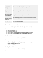
New in version 7.0:









You can now add multiple copies of behaviors to your runs and apply them to different
tree life history stages with different parameters.
The user manual has been rewritten to expand on basic ideas and help guide you through
run setup.
Data visualization charting controls have been simplified in order to help you manage all
the possible chart options for an output file.
A new menu option called Tools holds useful utilities for working with SORTIE-ND.
A new option in the "Tools" menu allows you to copy and rename detailed output files.
A new option in the "Tools" menu allows you to extract data from multiple output files at
the same time.
A "recent" charts button lets you find your favorite charts easily each time you load an
output file.
SORTIE-ND tracks open chart windows at the top of the screen so you can quickly pull
up the one you want.
A file history in the "File" menu keeps track of recently opened parameter and output
files.
What's New archive
Basic SORTIE modeling concepts
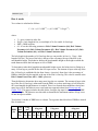
SORTIE is an individual-based forest simulator designed to study neighborhood processes. This
means that the trees in the forest are modeled individually, not as averages or spatial aggregates.
Each individual has a location in space. SORTIE specializes in modeling the interactions of trees
with their nearest neighbors to study local neighborhood dynamics.
SORTIE state data
The basic SORTIE model state is defined by the plot, trees, and grids. The plot is the underlying
location in which the simulation takes place. It has a particular size and shape, and attributes for
climate and geographic location. The trees are the individuals making up the forest on the plot.
Grids hold additional data that varies from place to place, such as soil chemistry or light level at
the forest floor. All of these together define the model state at a particular time.
Behaviors
The processes that act to change the model state are called behaviors. Behaviors often
correspond to biological processes. They are individually contained units, but often work
together to create a complex, interacting system. For instance, a simulation might consist of three
behaviors: a behavior to calculate light levels for trees, one to determine the amount of tree
growth as a result of the amount of light, and one to select trees to die if they grow too slowly.
Behaviors are placed in a certain order to correctly structure their interactions.
The simulation
Forests tend to operate on annual cycles, and so does SORTIE. The unit of time in SORTIE is
the timestep. It represents a set of one or more years. A single timestep consists of each behavior
acting once, in their defined order. The process is repeated for the number of timesteps that you
set, and that's a single simulation, or run.
The basic structure of the SORTIE system is very simple. Its power lies in its incredible
flexibility. Almost every aspect of the model is under direct user control.
The parameter file
When you start the SORTIE software, you are using a tool that helps you to define the state data
and behaviors that will make up a simulation. Once you have done this, you have created a
parameter file. The parameter file completely defines a run. You can load and run your
parameter file any time.
Setting up SORTIE-ND for your site
The major research projects involving SORTIE all began with multi year field studies to gather
data and analyze tree life cycle processes in the location being studied. This resulted in SORTIE
simulations that reflect as accurately as possible local conditions in the real world.
This means that there is no "standard" setup, and no database of tree species, sites, and
parameters to draw from. SORTIE was intended to study real locations, and that tends to mean
starting by finding out how trees behave at a study site.
This does not mean that you must start with field studies. Neither does it mean that you have to
study real places - SORTIE has also been used for purely theoretical work. What it means is that
you will need to gather a lot of information before you start.
Look at the example provided on the SORTIE website, read some of the SORTIE related
publications, and begin to build your parameter file. You'll quickly see what information you
need.
Plot
The plot in SORTIE is the simulation of the physical space in which the model runs. It has a size,
a climate, and a geographical location.
Plot size
You can think of the plot as a rectangle (although it's not really - more on that later). You tell the
plot what its east-west and north-south dimensions are. It's useful to keep your plot size in mind
when you are setting up your parameters and viewing your output, since many SORTIE values
are per hectare units. The size of your plot also makes a difference in run time - the larger the
plot, the longer the run. The absolute minimum size of a plot is 100 meters by 100 meters; 200
meters by 200 meters is a more realistic minimum. It is a careful balance to find a plot size big
enough to see the effects you are interested in but not so big that your runs take too long to be
practical. Since the length of the run depends on many other factors in addition to plot size, you
may need to tweak plot size a bit until you've found a good value.
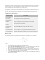
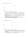
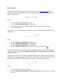
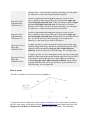
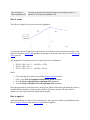
The SORTIE Coordinate System
SORTIE uses X-Y coordinates, starting at (0, 0), which is at the southwest corner of the plot.
Positive Y coordinates increase to the north; positive X coordinates increase to the east. There
are no negative plot location values. The coordinate values are in meters.
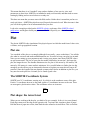
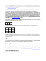
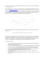
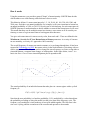
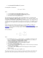
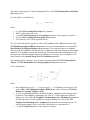
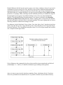
Plot shape: the torus forest
When you are working with the plot, you think of it as a rectangle. In fact, it is a torus (donut).
Each edge connects to the edge on the opposite side. To picture this, imagine a sheet of paper.
Roll the sheet of paper into a tube, then bend the tube around so its ends meet. This is what the
SORTIE forest looks like. The purpose of this shape is to eliminate edges in the forest. Trees
near the "edges" of the plot torus "see" trees on the far "edge" as being right next to them.
The torus shape is what controls the minimum plot size in SORTIE. Some processes in SORTIE
require searching a portion of the plot - for instance, to find all the trees in a given circle. If that
search took place over too great an area compared to the size of the plot, it would run the risk of
searching "around the world." It would work its way around the torus and back to (and past) the
place it started, finding the same trees multiple times.
Plot climate and location
The plot also has a climate and a geographical location. Some behaviors use this information but
others do not. This information is ignored if it is not needed.
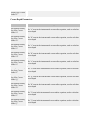
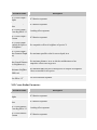
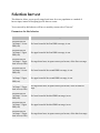
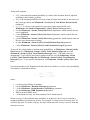
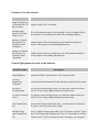
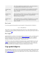
Plot parameters
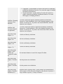
Parameter name
Description</th
Number of timesteps
The number of timesteps to run the model. See more on timesteps.
Number of years per
timestep
The length of the timestep, in years. It is recommended that this value be
a whole number.
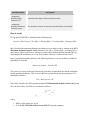
Random seed
An integer to use as the seed for SORTIE's random number generator.
Zero means that SORTIE chooses its own new seed every time, and
repeat runs with the same parameter file will come out different. Any
non-zero value triggers one particular sequence of random numbers. In
that case, repeat runs with the same parameter file will be the same.
Plot Length in the X
(E-W) Direction, in
meters
The length of the plot in the east-west direction, in meters.
Plot Length in the Y
(N-S) Direction, in
meters
The length of the plot in the north-south direction, in meters.
Plot Latitude, in
decimal degrees
The plot latitude, expressed in decimal degrees (i.e. 39.10). This
information may not be needed in the run, depending on the behaviors
that you select; if it is not needed, this value will be ignored.
Mean Annual
The mean annual precipitation of the plot, in millimeters. This
Precipitation, mm
information may not be needed in the run, depending on the behaviors
that you select; if it is not needed, this value will be ignored.
Mean Annual
Temperature,
degrees C
The mean annual temperature of the plot, in degrees Celsius. This
information may not be needed in the run, depending on the behaviors
that you select; if it is not needed, this value will be ignored.
Timesteps and run length
A run is a single model simulation. It starts at time zero and continues until its defined endpoint
is reached. A run is defined by its parameter file. This tells the model how long to run, and what
to do during the run.
Timesteps
The basic time unit in the run is the timestep. You set the length and number of the timesteps.
Each timestep, the model asks each behavior to do its work, whatever that work may be. The
behaviors are run in the order in which they are listed in the parameter file. (You can see the
order using the Model flow window.) The model counts off the timesteps until it has finished the
specified number, then cleans up its memory and shuts down.
The length of a timestep is defined in years. Setting a longer timestep means that you can
simulate long stretches of time more quickly and with less computer processing time. For
example, you could create two parameter files using the same behavior set, each for a run of 100
timesteps. Parameter file A has a timestep length of one year. Parameter file B has a timestep
length of five years. Both will take about the same amount of time to run, because each behavior
is called upon the same number of times in each run - once per timestep. However, at the end of
the run for parameter file A, 100 virtual years will have passed, while for parameter file B, 500
years will have passed. The forests at the end of each of the two runs would probably look quite
different.
There is, of course, a tradeoff. When a timestep is more than one year long, behaviors do their
best to approximate what happens in those successive years. They can only do that based on the
model state at the beginning of the timestep, without knowing how things might change from
year to year because of other behaviors. Depending on the simulation, this approximation might
create results that are very different from the results that would have come from a single year
timestep simulation.
Choosing a timestep length
A one year timestep is the default choice, because it makes sure that SORTIE can model short
term interactions directly instead of approximating them. There are two main reasons for
choosing a multi-year timestep: shortening processing time for runs that are otherwise
unreasonably long, and using parameters that have been estimated for multiple years and cannot
easily be rescaled.
That second reason can only apply in rare situations, since most behaviors require parameters
scaled to one year, even when a multi-year timestep is being used. Study the documentation for
each behavior you want to use. In some cases, behaviors insist on a particular timestep length to
ensure proper functioning.
It is difficult to guess how long a parameter file will take to run, so first, try running your
parameter file with a one year timestep. If you're happy with how long it took SORTIE to run
your parameter file, use one year timesteps.
If you think you might need a multi-year timestep, check the behavior documentation again.
Each behavior will describe how it handles timesteps of different lengths. Make sure you think
the approach is reasonable. Then, try running two versions of your parameter file, one with one
year timesteps and one with multi-year timesteps, with both files modeling the same amount of
total time (for instance, 100 one year timesteps and 20 five year timesteps). Make sure you think
the difference is reasonable.
What is a tree?
The basic unit of data in the model is the tree. A model tree is a collection of attributes
describing one individual. The attributes include location in the plot, species, life history stage,
and size. Additional attributes are added as needed for the use of the particular set of behaviors in
a run.
Location and species for a tree never change. Life history stage transitions are handled
automatically as a tree moves through its lifecycle. Tree size and shape are managed according to
allometry settings. Behavior-specific attributes are managed by the appropriate behavior.
You work with these attributes when you select data for output or work with tree maps when
setting up run initial conditions.
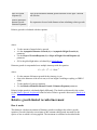
How trees are organized - the tree population
Trees are organized by location and size in what is called the tree population. The tree population
divides up the plot into 8 m by 8 m grid cells, and tracks the trees in each cell by height.
The tree population is where the list of tree species is defined. It tracks all of the allometry
relationships for each of these species and manages life history stage transitions and attribute
updates for individual trees.
Tree life history stages and transitions
Tree life history stage (also referred to as tree type), along with species, is the basic way to
classify trees. When you set up behaviors for a run, you tell each behavior which trees to act on
by species and type. There is support for seven tree life history stages in the model:







Seed.
Seedling. Seedlings are defined as trees less than the height set in the parameter Max
Seedling Height (meters) (normally 1.35 meters, thus seedlings have no DBH). Their
primary size measurement is the diameter at 10 cm height (diam10).
Sapling. Saplings are defined as having a DBH greater than 0 and less than the
Minimum adult DBH defined in the tree parameters. Seedlings and saplings are
sometimes referred to collectively as "juveniles".
Adult. Adults are defined as having a DBH equal to or greater than the Minimum adult
DBH defined in the tree parameters.
Stump. Stumps are saplings or adults that have been cut by the Harvest behavior.
Snag. Snags are standing dead trees. They can be produced when saplings and adults die
due to normal tree mortality or a disturbance event, such as disease. Only adult trees
become snags. See below for more on how trees become snags.
Woody debris. Woody debris comes from fallen snags. Currently, no behavior uses
woody debris and this is a placeholder stage only. It is not created at this time.
Tree life history stage transitioning - growth
Seed to seedling. Seeds are modeled only as aggregates, not individuals. Seeds become
individual seedlings when they are processed by an establishment behavior.
Seedling to sapling. When a seedling reaches the maximum seedling height set for its species, it
becomes a sapling. The diam10 value is converted to a DBH value, which is then used to
calculate the rest of the sapling's new dimensions. Since height is re-calculated with a different
equation and input parameters, there may be a discontinuity in height values right around the
seedling/sapling transition point. If a species uses different allometric relationships for its
saplings and adults, another discontinuity may occur at the time of this transition as well. For
more on the allometric relationships and how they are calculated, see the Allometry topic. (The
automatic updating of these allometric relationships during the growth phase can be overridden.
For more, see the Growth behaviors topic.)
Sapling to adult. When a sapling's DBH reaches the minimum adult DBH for its species, it
becomes an adult.
Tree life history stage transitioning - death
Death also produces tree life history stage transitions. Behaviors can request to a tree population
that a tree be killed. How the tree population responds to this request depends on the type of tree,
the reason for death, and the type of run.
Mortality reasons
The reasons why a tree is killed are:





Natural mortality
Harvest
Insects
Fire
Disease
Check the documentation for your chosen disturbance behaviors and mortality behaviors for
more information on which codes will apply to your run.
There are life history stages for dead trees, but a run may not be set up to handle them. The tree
population takes this into account. It examines the run to see if any behaviors directly deal with
stumps and snags. If either is the case, the run is classified as "stump aware" and/or "snag
aware".
Here's what happens to a tree to be killed in different situations:







If a tree is a seedling, it is deleted from memory no matter why it died.
If a tree is a sapling or adult killed in a harvest, and the run is "stump aware", the tree is
converted to a stump.
Saplings killed for any other reason, or by harvest in a run that is not "stump aware", are
deleted from memory.
If the tree is an adult killed by harvest and the run is not "stump aware", it is deleted from
memory.
If the tree is an adult killed for any reason other than harvest, and the run is "snag aware",
the tree is converted to a snag.
If the tree is an adult killed for any reason other than harvest, and the run is NOT "snag
aware", the tree is removed from memory.
If the tree is already a snag, it is removed from memory.
Stumps exist only for the timestep in which they were created, and then disappear.
You can include information on dead trees in output files. For the purposes of output, dead trees
are those which have been removed from memory and are no longer interacting with the model
in any way. In this case, a snag is considered alive, although a tree that produced a snag will
show up in output mortality records in the timestep in which it died to become a snag. Then the
snag would show up again when it was finally removed from the model.
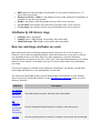
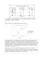
Allometry
The allometry relationships govern a tree's size and shape.
Tree size attributes





DBH (diameter at breast height) is the diameter of a tree trunk in centimeters at 1.35
meters above the ground.
Diameter at 10 cm, or diam10, is the diameter of a tree trunk, measured in centimeters, at
a height of 10 cm above the ground.
Height is the distance from the ground to the top of the crown, in meters.
Crown radius is the distance from the trunk to the edge of the crown, in meters.
Crown depth is the distance from the top to the bottom of the crown, in meters.
Attributes by life history stage



Seedlings: diam10 and height.
Saplings: diam10, DBH, height, crown radius, and crown depth.
Adults and snags: DBH, height, crown radius, and crown depth.
How size and shape attributes are used
Many behaviors do their work using equations that are functions of tree size in some way.
Diameter is by far the most important attribute. Other dimensions may or may not be used in a
run, depending on the set of chosen behaviors. How important it is to get the allometric
relationships correct depends on how they will be used. Check the documentation of your chosen
behaviors. If, for instance, crown shape is not used, it doesn't really matter what relationships
you assign.
Trees are not required to conform to their allometric relationships. For instance, growth many
cause height and diameter to vary independently of each other.
You choose the relationship used by each life history stage of each species for each attribute.
These can be freely mixed-and-matched. Use the Edit Allometry Functions window to set the
allometry functions.
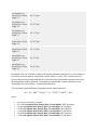
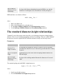
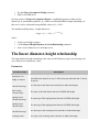
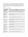
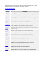
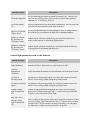
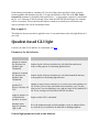
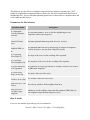
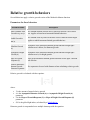
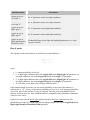
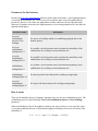
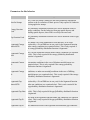
Function
Description
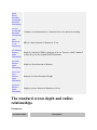
The standard
crown depth
and radius
relationships
Crown dimensions are power functions of tree dimensions.
The
ChapmanRichards
crown depth
and radius
relationships
Uses the Chapman-Richards function to calculate crown dimensions.
The non-
Uses non-spatial measures of density to calculate crown radius and crown depth.
spatial
density
dependent
crown depth
and radius
relationships
The NCI
crown depth
and radius
relationships
Calculates crown dimensions as a function of tree size and local crowding.
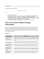
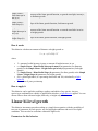
DBH diameter at
10 cm
relationship
DBH is a linear function of diameter at 10 cm.
The standard
diameterheight
relationships
Height is a function of DBH or diameter at 10 cm. These are called "standard"
because they were the original SORTIE functions.
The linear
diameterheight
relationship
Height is a linear function of diameter.
The reverse
linear
diameterheight
relationship
Diameter is a linear function of height.
The power
diameterheight
relationship
Height is a power function of diameter at 10 cm.
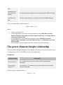
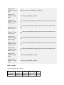
The standard crown depth and radius
relationships
Parameters
Parameter name
Description
Crown Height
Exponent
The exponent in the standard equation for calculating crown depth.
Crown Radius
Exponent
The exponent in the standard equation for determining the crown radius.
Slope of Asymptotic
Crown Height
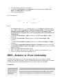
Slope of the standard equation for determining crown depth.
Slope of Asymptotic
Crown Radius
Slope of the standard equation for determining crown radius.
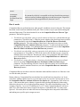
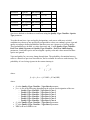
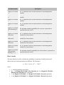
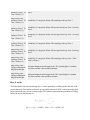
Crown radius is calculated as:
rad = C1 * DBH a
where:




rad is the crown radius, in meters
C1 is the Slope of Asymptotic Crown Radius parameter
a is the Crown Radius Exponent parameter
DBH is the tree's DBH, in cm
Crown radius is limited to a maximum of 10 meters.
Crown depth is calculated as
ch = C2 * height b
where




ch is the distance from the top to the bottom of the crown cylinder, in meters
C2 is the Slope of Asymptotic Crown Height parameter
height is the tree's height in meters
b is the Crown Height Exponent parameter
The Chapman-Richards crown depth and
radius relationships
Crown Depth Parameters
Parameter name
Description
Chapman-Richards
Asymptotic Crown
Height
The asymptotic crown depth (or length), in m, of the Chapman-Richards
crown depth equation.
Chapman-Richards
Crown Height
Intercept
The intercept of the Chapman-Richards crown depth equation. This
represents the crown depth, in m, of the smallest possible sapling.
Chapman-Richards
Crown Height Shape
1 (b)
The first shape parameter, b, of the Chapman-Richards crown depth
equation.
Chapman-Richards
Crown Height Shape
2 (c)
The second shape parameter, c, of the Chapman-Richards crown depth
equation.
Crown Radius Parameters
Parameter name
Description
Chapman-Richards
Asymptotic Crown
Radius
The asymptotic crown radius, in m, of the Chapman-Richards crown
radius equation.
Chapman-Richards
Crown Radius
Intercept
The intercept of the Chapman-Richards crown radius equation. This
represents the crown radius, in m, of the smallest possible sapling.
Chapman-Richards
Crown Radius Shape
1 (b)
The first shape parameter, b, of the Chapman-Richards crown radius
equation.
Chapman-Richards
Crown Radius Shape
2 (c)
The second shape parameter, c, of the Chapman-Richards crown radius
equation.
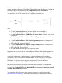
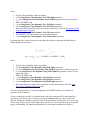
The Chapman-Richards equation for calculating crown radius is:
rad = i + a (1 - e -b * DBH) c
where



rad is the crown radius, in meters
DBH is the tree's DBH, in cm
i is the Chapman-Richards Crown Radius Intercept parameter, which represents the
crown radius of the smallest possible sapling



a is the Chapman-Richards Asymptotic Crown Radius parameter
b is the Chapman-Richards Crown Radius Shape 1 (b) parameter
c is the Chapman-Richards Crown Radius Shape 2 (c) parameter
The Chapman-Richards equation for calculating crown depth is:
ch = i + a (1 - e -b * H) c
where






ch is the distance from the top to the bottom of the crown cylinder, in meters
H is the tree's height, in m
i is the Chapman-Richards Crown Height Intercept parameter, which represents the
crown depth of the smallest possible sapling
a is the Chapman-Richards Asymptotic Crown Height parameter
b is the Chapman-Richards Crown Height Shape 1 (b) parameter
c is the Chapman-Richards Crown Height Shape 2 (c) parameter
The non-spatial density dependent crown
depth and radius relationships
The density dependent equations for crown radius and crown depth use non-spatial measures of
density to influence crown radius and crown depth. Density is measured across the plot as a
whole, not locally (thus "non-spatial").
Crown Radius Parameters
Parameter name
Description
Non-Spatial Density
Dep. Inst. Crown
Height "a"
The "a" term in the instrumental crown depth equation, used to calculate
crown radius
Non-Spatial Density
Dep. Inst. Crown
Height "b"
The "b" term in the instrumental crown depth equation, used to calculate
crown radius
Non-Spatial Density
Dep. Inst. Crown
Height "c"
The "c" term in the instrumental crown depth equation, used to calculate
crown radius
Non-Spatial Density
Dep. Inst. Crown
Height "d"
The "d" term in the instrumental crown depth equation, used to calculate
crown radius
Non-Spatial Density
Dep. Inst. Crown
Height "e"
The "e" term in the instrumental crown depth equation, used to calculate
crown radius
Non-Spatial Density
Dep. Inst. Crown
Height "f"
The "f" term in the instrumental crown depth equation, used to calculate
crown radius
Non-Spatial Density
Dep. Inst. Crown
Height "g"
The "g" term in the instrumental crown depth equation, used to calculate
crown radius
Non-Spatial Density
Dep. Inst. Crown
Height "h"
The "h" term in the instrumental crown depth equation, used to calculate
crown radius
Non-Spatial Density
Dep. Inst. Crown
Height "i"
The "i" term in the instrumental crown depth equation, used to calculate
crown radius
Non-Spatial Density
Dep. Inst. Crown
Height "j"
The "j" term in the instrumental crown depth equation, used to calculate
crown radius
Non-Spatial Exp.
Density Dep. Crown
Radius "D1"
The "D1" term
Non-Spatial Exp.
Density Dep. Crown
Radius "a"
The "a" term
Non-Spatial Exp.
Density Dep. Crown
Radius "b"
The "b" term
Non-Spatial Exp.
Density Dep. Crown
Radius "c"
The "c" term
Non-Spatial Exp.
Density Dep. Crown
Radius "d"
The "d" term
Non-Spatial Exp.
Density Dep. Crown
Radius "e"
The "e" term
Non-Spatial Exp.
The "f" term
Density Dep. Crown
Radius "f"
Crown Depth Parameters
Parameter name
Description
Non-Spatial Density
Dep. Inst. Crown
Radius "a"
The "a" term in the instrumental crown radius equation, used to calculate
crown depth
Non-Spatial Density
Dep. Inst. Crown
Radius "b"
The "b" term in the instrumental crown radius equation, used to calculate
crown depth
Non-Spatial Density
Dep. Inst. Crown
Radius "c"
The "c" term in the instrumental crown radius equation, used to calculate
crown depth
Non-Spatial Density
Dep. Inst. Crown
Radius "d"
The "d" term in the instrumental crown radius equation, used to calculate
crown depth
Non-Spatial Density
Dep. Inst. Crown
Radius "e"
The "e" term in the instrumental crown radius equation, used to calculate
crown depth
Non-Spatial Density
Dep. Inst. Crown
Radius "f"
The "f" term in the instrumental crown radius equation, used to calculate
crown depth
Non-Spatial Density
Dep. Inst. Crown
Radius "g"
The "g" term in the instrumental crown radius equation, used to calculate
crown depth
Non-Spatial Density
Dep. Inst. Crown
Radius "h"
The "h" term in the instrumental crown radius equation, used to calculate
crown depth
Non-Spatial Density
Dep. Inst. Crown
Radius "i"
The "i" term in the instrumental crown radius equation, used to calculate
crown depth
Non-Spatial Density
Dep. Inst. Crown
Radius "j"
The "j" term in the instrumental crown radius equation, used to calculate
crown depth
Non-Spatial Log.
Density Dep. Crown
Height "a"
The "a" term
Non-Spatial Log.
Density Dep. Crown
Height "b"
The "b" term
Non-Spatial Log.
Density Dep. Crown
Height "c"
The "c" term
Non-Spatial Log.
Density Dep. Crown
Height "d"
The "d" term
Non-Spatial Log.
Density Dep. Crown
Height "e"
The "e" term
Non-Spatial Log.
Density Dep. Crown
Height "f"
The "f" term
Non-Spatial Log.
Density Dep. Crown
Height "g"
The "g" term
In addition to the use of density variables, the density dependent equations for crown width uses
an estimate of crown depth as a dependent variable (and vice versa). This estimated value of
crown width and crown depth (radi and chi) used in the density dependent equations come from
the instrumental variable equations. Calculating the instrumental variables equations avoids
"uncoupling" the crown radius - crown depth relationship.
The non-spatial exponential density dependent crown radius function is:
rad = D1 * DBH a * Height b * chi c * STPH d * BAPH e * BAL f
where:







rad is the crown radius, in meters
D1 is the Non-Spatial Exp. Density Dep. Crown Radius "D1" parameter
a is the Non-Spatial Exp. Density Dep. Crown Radius "a" parameter
b is the Non-Spatial Exp. Density Dep. Crown Radius "b" parameter
c is the Non-Spatial Exp. Density Dep. Crown Radius "c" parameter
d is the Non-Spatial Exp. Density Dep. Crown Radius "d" parameter
e is the Non-Spatial Exp. Density Dep. Crown Radius "e" parameter







f is the Non-Spatial Exp. Density Dep. Crown Radius "f" parameter
DBH is the tree's DBH, in cm
Height is the tree height, in meters
chi is the instrumental crown depth of the target tree, in meters, calculated using the
function below
STPH is number of stems per hectare of adult trees within the entire plot
BAPH is the basal area, in m2 per hectare, of adult trees within the entire plot
BAL is the sum of the basal area of all trees taller than the height of the target tree, in m2
per hectare
The instrumental equation for calculating chi is as follows:
chi = a + b * DBH + c * Height + d * DBH 2 + e * Height 2 + f / DBH + g * STPH + h * BAPH
+ i * BAL + j * (Height / DBH)
where:















a is the Non-Spatial Density Dep. Inst. Crown Height "a" parameter
b is the Non-Spatial Density Dep. Inst. Crown Height "b" parameter
c is the Non-Spatial Density Dep. Inst. Crown Height "c" parameter
d is the Non-Spatial Density Dep. Inst. Crown Height "d" parameter
e is the Non-Spatial Density Dep. Inst. Crown Height "e" parameter
f is the Non-Spatial Density Dep. Inst. Crown Height "f" parameter
g is the Non-Spatial Density Dep. Inst. Crown Height "g" parameter
h is the Non-Spatial Density Dep. Inst. Crown Height "h" parameter
i is the Non-Spatial Density Dep. Inst. Crown Height "i" parameter
j is the Non-Spatial Density Dep. Inst. Crown Height "j" parameter
DBH is the tree's DBH, in cm
Height is the tree height, in meters
STPH is number of stems per hectare of adult trees within the entire plot
BAPH is the basal area, in m2 per hectare, of adult trees within the entire plot
BAL is the sum of the basal area of all trees taller than the height of the target tree, in m2
per hectare
The non-spatial logistic density dependent crown depth function is:
where:




ch is the crown depth, in meters
height is the tree's height, in m
a is the Non-Spatial Log. Density Dep. Crown Height "a" parameter
b is the Non-Spatial Log. Density Dep. Crown Height "b" parameter










c is the Non-Spatial Log. Density Dep. Crown Height "c" parameter
d is the Non-Spatial Log. Density Dep. Crown Height "d" parameter
e is the Non-Spatial Log. Density Dep. Crown Height "e" parameter
f is the Non-Spatial Log. Density Dep. Crown Height "f" parameter
g is the Non-Spatial Log. Density Dep. Crown Height "g" parameter
DBH is the tree's DBH, in cm
radi is the instrumental crown radius of the target tree, in meters, calculated using the
function below
STPH is number of stems per hectare of adult trees within the entire plot
BAPH is the basal area, in m2 per hectare, of adult trees within the entire plot
BAL is the sum of the basal area of all trees taller than the height of the target tree, in m2
per hectare
The instrumental equation for calculating radi is as follows:
radi = a + b * DBH + c * Height + d * DBH 2 + e * Height 2 + f / DBH + g * STPH + h *
BAPH + i * BAL + j * (Height / DBH)
where:















a is the Non-Spatial Density Dep. Inst. Crown Radius "a" parameter
b is the Non-Spatial Density Dep. Inst. Crown Radius "b" parameter
c is the Non-Spatial Density Dep. Inst. Crown Radius "c" parameter
d is the Non-Spatial Density Dep. Inst. Crown Radius "d" parameter
e is the Non-Spatial Density Dep. Inst. Crown Radius "e" parameter
f is the Non-Spatial Density Dep. Inst. Crown Radius "f" parameter
g is the Non-Spatial Density Dep. Inst. Crown Radius "g" parameter
h is the Non-Spatial Density Dep. Inst. Crown Radius "h" parameter
i is the Non-Spatial Density Dep. Inst. Crown Radius "i" parameter
j is the Non-Spatial Density Dep. Inst. Crown Radius "j" parameter
DBH is the DBH of the tree, in cm
Height is the tree height, in meters
STPH is number of stems per hectare of adult trees within the entire plot
BAPH is the basal area, in m2 per hectare, of adult trees within the entire plot
BAL is the sum of the basal area of all trees taller than the height of the target tree, in m2
per hectare
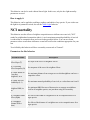
The NCI crown depth and radius
relationships
This calculates crown dimensions as a function of tree size and local crowding. The equations
are the same for crown depth and crown radius, but they each have separate parameters.
NCI Crown Depth Parameters
Parameter name
Description
NCI Crown Depth Alpha
NCI function exponent.
NCI Crown Depth Beta
NCI function exponent.
NCI Crown Depth Crowding Effect "n"
Crowding effect exponent.
NCI Crown Depth Gamma
NCI function exponent.
NCI Crown Depth
Lambda for Species
X Neighbors
The competitive effect of neighbors of species X.
NCI Crown Depth Max Potential Depth
(m)
The maximum possible value for crown depth, in m.
NCI Crown Depth The maximum distance, in m, at which a neighboring tree has
Max Search Distance
competitive effects on a target tree.
for Neighbors (m)
NCI Crown Depth Minimum Neighbor
DBH (cm)
The minimum DBH for trees of that species to compete as neighbors.
Values are needed for all species.
NCI Crown Depth Size Effect "d"
Size effect function exponent.
NCI Crown Radius Parameters
Parameter name
Description
NCI Crown Radius Alpha
NCI function exponent.
NCI Crown Radius Beta
NCI function exponent.
NCI Crown Radius Crowding Effect "n"
Crowding effect exponent.
NCI Crown Radius Gamma
NCI function exponent.
NCI Crown Radius
Lambda for Species
X Neighbors
The competitive effect of neighbors of species X.
NCI Crown Radius Max Potential
Radius (m)
The maximum possible value for crown radius, in m.
NCI Crown Radius The maximum distance, in m, at which a neighboring tree has
Max Search Distance
competitive effects on a target tree.
for Neighbors (m)
NCI Crown Radius Minimum Neighbor
DBH (cm)
The minimum DBH for trees of that species to compete as neighbors.
Values are needed for all species.
NCI Crown Radius Size Effect "d"
Size effect function exponent.
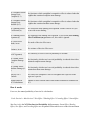
The crown dimensions are calculated as:
CR / CD = [Max CR / Max CD] * Size Effect * Crowding Effect
where:




CR is the crown radius, in m
CD is the crown depth, in m
Max CR is the NCI Crown Radius - Max Potential Radius (m) parameter
Max CD is the NCI Crown Depth - Max Potential Depth (m) parameter
Size Effect is calculated as:
SE = 1 - exp(-d * DBH)
where:



SE is the size effect, between 0 and 1
d is either the NCI Crown Depth - Size Effect "d" parameter or the NCI Crown
Radius - Size Effect "d" parameter
DBH is the tree's DBH, in cm
Crowding Effect is calculated as:
CE = exp(-n * NCI)
where:



CE is the crowding effect, between 0 and 1
n is the NCI Crown Radius - Crowding Effect "n" parameter or the NCI Crown
Depth - Crowding Effect "n" parameter
NCI is calculated as below
NCI is calculated as:
where:








the calculation sums over j = 1...S species and k = 1...N neighbors of each species of at
least a DBH of NCI Crown Radius - Minimum Neighbor DBH or NCI Crown Depth
Minimum Neighbor DBH, in cm, out to a distance of NCI Crown Radius - Max
Search Distance for Neighbors (m) or NCI Crown Radius - Max Search Distance for
Neighbors (m)
α is the NCI Crown Radius - Alpha parameter or the NCI Crown Depth - Alpha
parameter
β is the NCI Crown Radius - Beta parameter or the NCI Crown Depth - Beta
parameter
γ is the NCI Crown Radius - Gamma parameter or the NCI Crown Depth - Gamma
parameter
λik is the NCI Crown Radius Lambda for Species X Neighbors parameter or the NCI
Crown Depth Lambda for Species X Neighbors for the target species relative to the kth
neighbor's species
DBHjk is the DBH of the kth neighbor, in cm
DBHt is the DBH of the target tree for which to calculate crown dimensions, in cm
distanceik is distance from target to neighbor, in m
DBH - diameter at 10 cm relationship
Seedlings use the diameter at 10 cm as their primary indicator of size, and have no DBH.
Saplings use both DBH and diam10. The use of both measurements by saplings helps to maintain
continuity between the seedling and adult life history stages. Adults use only DBH.
Parameters
Parameter name
Intercept of DBH to
Diameter at 10 cm
Relationship
Description
The intercept of the linear relationsip between the DBH, in cm, and the
diameter at 10 cm height, in cm, in small trees. Used by all species.
Slope of DBH to
Diameter at 10 cm
Relationship
The slope of the linear relationship between the DBH, in cm, and the
diameter at 10 cm height, in cm, in small trees. Used by all species.
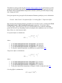
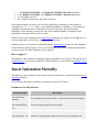
DBH and diam10 are related as follows:
DBH = (diam10 * R) + I
where




DBH is the DBH in cm
diam10 is the diameter at 10 cm height, in cm
R is the Slope of DBH to Diameter at 10 cm Relationship parameter
I is the Intercept of DBH to Diameter at 10 cm Relationship parameter
The standard diameter-height relationships
"Standard" is one of the names used to describe a set of allometric functions relating height to
diameter. There is one for adults and saplings, and one for seedlings. These are called "standard"
because they were the original SORTIE functions and until recently were the only choices.
Parameters
Parameter name
Description
Maximum Tree
Height, in meters
The maximum tree height for a species, in meters. No tree, no matter
what allometric function it uses, is allowed to get taller than this. Used by
all species.
Slope of Asymptotic
Height
Exponential decay term in the adult and sapling standard function for
DBH and height.
Slope of HeightDiameter at 10 cm
Relationship
The slope of the seedling standard function for diameter at 10 cm and
height.
The standard sapling and adult DBH - height function is:
height = 1.35 + (H1 - 1.35)(1 - e-B*DBH)
where:


height is tree height in meters
H1 is the Maximum Tree Height, in m parameter


B is the Slope of Asymptotic Height parameter
DBH is tree DBH in cm
In some articles, B (Slope of Asymptotic Height) is a published parameter. Other articles
instead use H1 and another parameter, H2, which was called the DBH to height relationship. In
this case, B can be calculated from published values as B = H2/H1.
The standard seedling diam10 - height function is:
height = 0.1 + 30*(1 - e(-α * diam10))
where:



height is tree height in meters
α is the Slope of Height-Diameter at 10 cm Relationship parameter
diam10 is tree diameter at 10 cm height, in cm
The linear diameter-height relationship
The linear diameter-height relationship is the same for all life history stages, but each stage can
use a different set of parameter values.
Parameters
Parameter name
Description
Maximum Tree
Height, in meters
The maximum tree height for a species, in meters. No tree, no matter
what allometric function it uses, is allowed to get taller than this. Used by
all species.
Adult Linear
Function Intercept
The intercept of the adult linear function for DBH and height.
Adult Linear
Function Slope
The slope of the adult linear function for DBH and height.
Sapling Linear
Function Intercept
The intercept of the sapling linear function for DBH and height.
Sapling Linear
Function Slope
The intercept of the sapling linear function for DBH and height.
Seedling Linear
Function Intercept
The intercept of the seedling linear function for DBH and height.
Seedling Linear
The slope of the seedling linear function for DBH and height.
Function Slope
The linear diam - height function is:
height = a + b * diam
where:




height is tree height, in m
a is the appropriate linear intercept parameter (either Adult Linear Function Intercept,
Sapling Linear Function Intercept, or Seedling Linear Function Intercept)
b is the appropriate linear slope parameter (either Adult Linear Function Slope, Sapling
Linear Function Slope, or Seedling Linear Function Slope)
diam is DBH (in cm) for saplings and adults, or diam10 (in cm) for seedlings
The reverse linear diameter-height
relationship
The reverse linear diameter-height relationship is the same for all life history stages, but each
stage can use a different set of parameter values. The name comes from the fact that it is almost
the same as the linear function, but with height and diameter switched. In other words, in the
linear function, height is a linear function of diameter. In the reverse linear function, diameter is
a linear function of height.
Parameters
Parameter name
Maximum Tree
Height, in meters
Description
The maximum tree height for a species, in meters. No tree, no matter
what allometric function it uses, is allowed to get taller than this. Used by
all species.
Adult Reverse Linear
The intercept of the adult reverse linear function for DBH and height.
Function Intercept
Adult Reverse Linear
The slope of the adult reverse linear function for DBH and height.
Function Slope
Sapling Reverse
Linear Function
Intercept
The intercept of the sapling reverse linear function for DBH and height.
Sapling Reverse
Linear Function
The slope of the sapling reverse linear function for DBH and height.
Slope
Seedling Reverse
Linear Function
Intercept
The intercept of the seedling reverse linear function for DBH and height.
Seedling Reverse
Linear Function
Slope
The slope of the seedling reverse linear function for DBH and height.
The reverse linear diam - height function is:
height = (diam - a) / b
where:




height is tree height, in m
a is the appropriate reverse linear intercept parameter (either Adult Reverse Linear
Function Intercept, Sapling Reverse Linear Function Intercept, or Seedling Reverse
Linear Function Intercept)
b is the appropriate reverse linear slope parameter (either Adult Reverse Linear
Function Slope, Sapling Reverse Linear Function Slope, or Seedling Reverse Linear
Function Slope)
diam is DBH (in cm) for saplings and adults, or diam10 (in cm) for seedlings
The power diameter-height relationship
The power diameter-height relationship relates height and diameter with a power function. Since
it uses diameter at 10 cm, NOT DBH, it is active for saplings only.
Parameters
Parameter name
Description
Power Function "a"
The "a" parameter in the power function for the height-diameter
relationship.
Power Function
Exponent "b"
The exponent, or "b" parameter, in the power function for the heightdiameter relationship.
The power diam - height function is:
height = a * d10 b
where:




height is tree height, in m
a is the Power Function "a" parameter
b is the Power Function Exponent "b" parameter
d10 is diameter at 10 cm (in cm)
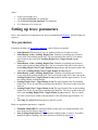
Setting up trees: parameters
Here is the complete list of parameters for the tree population and allometry. Not all of them are
required.
Tree parameters
Parameters dealing with tree initial conditions - none of these are required:







Initial Densities The density of trees, in number per hectare, for that size class.
Initial Density (#/ha) - Seedling Height Class 1 Number of seedlings per hectare to
create in the first seedling height class. The lower bound of this class is 0 cm and the
upper bound is the value in the Seedling Height Class 1 Upper Bound, in cm
parameter.
Initial Density (#/ha) - Seedling Height Class 2 Number of seedlings per hectare to
create in the second seedling height class. The lower bound of this class is the value in
the Seedling Height Class 1 Upper Bound, in cm parameter and the upper bound is the
value in the Seedling Height Class 2 Upper Bound, in cm parameter.
Initial Density (#/ha) - Seedling Height Class 3 Number of seedlings per hectare to
create in the third seedling height class. The lower bound of this class is the value in the
Seedling Height Class 2 Upper Bound, in cm parameter and the upper bound is 135 cm
(the tallest possible seedling height).
Seedling Height Class 1 Upper Bound, in cm The upper bound of the first seedling
height class, in cm, for specifying seedling initial densities. The lower bound of the size
class is 0.
Seedling Height Class 2 Upper Bound, in cm The upper bound of the second seedling
height class, in cm, for specifying seedling initial densities. The lower bound of the size
class is the Seedling Height Class 2 Upper Bound, in cm parameter. There is a third
size class, whose lower bound is this parameter's value and whose upper bound is 135
cm.
Tree Map To Add As Text External tree map file to add.
Basic tree population parameters - required:


Minimum Adult DBH The minimum DBH at which trees are considered adults. (See
more about tree life history stages here.)
Max Seedling Height (meters) The maximum seedling height, in meters. Trees taller
than this height are saplings. (See more about tree life history stages here.)

New Seedling Diameter at 10 cm The average diameter at 10 cm height value for newly
created seedlings, when another size is not specified. Actual values are randomized
slightly around this value.
In addition to the values listed in the parameter window, the tree population also keeps the list of
species and size classes. These can be edited in the Tree population - edit species list window
and Tree population - edit initial density size classes window.
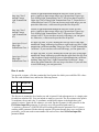
Tree initial conditions
Tree initial conditions are the trees in the SORTIE forest when a simulation begins. The initial
conditions are often of vital importance to how a run develops.
There are two ways to add trees at the beginning of the run, and they can be used together or
separately. The first is to ask the model to create trees for you according to your chosen species
composition and size structure. The second way is to directly list a particular set of trees in a tree
map.
Defining initial conditions using species composition and size
structure
For saplings and adults, you can set up DBH size classes and enter the desired density in each
size class. To set up size classes, use the Edit size classes window. You can define as many size
classes as you want. The values that you enter are the upper bounds of each class. Once you have
defined all of your size classes, you can enter the desired number of stems per hectare for each
species for each class in the tree parameters which you edit using the Parameters window.
There are two different ways to enter seedling densities. Defining a DBH size class of zero gives
you a line for entering stems per hectare of seedlings. These seedlings will be brand new, with
sizes approximating the value in the New Seedling Diameter at 10 cm tree parameters. If you
would like more control over seedling sizes, you can define three height classes densities for
each in the tree parameters.
The resulting trees are randomly distributed around the plot. Actual sizes are chosen randomly
from a uniform distribution within each size class.
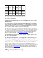
Tree maps
Tree maps are lists of individual trees. You can add one or more maps to your parameter file.
The maps can come from detailed output files from other runs, or you can make your own tabdelimited tree maps. The preferred method of incorporating a tree map to a run is to add it
directly into a parameter file. However, if the number of trees is very large, it may make the
XML file too big to read. In this case, a text tree file's filename can be added to the parameter file
instead and SORTIE can read the trees directly from the file.
Choosing how to set up the initial conditions
In most cases, you would define your initial conditions using DBH size classes. They are simple
to define and describe. There are cases where you would need a tree map. For example:




You intend to model a particular real-life plot
You want to use a mid-run timestep of another simulation as the starting point of a new
simulation
You want a particular spatial pattern of trees instead of a random distribution
You want to do a set of simulations that all start out exactly the same way
You can mix the two methods as well. If you have a tree map of adults you'd like to use, you can
add seedlings and saplings using size classes.
It is important to consider initial conditions for juveniles. It can take awhile for seed dispersal,
establishment, and recruitment to create juveniles in a run. You may see strange behavior in your
first timesteps if you're missing a whole life cycle stage in your tree population.
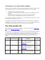
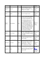
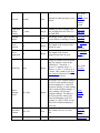
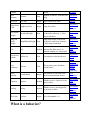
Tree data member list
This is a list of the possible data that a tree can have. You can save this data in a detailed output
file by using the Setup tree save options window.
Not all data is always available. Certain sets of behaviors require additional information about a
tree. One of the ways in which behaviors communicate with one another is by defining new
pieces of data for trees and then setting and reading values for those data. A piece of data created
by a behavior is only attached to those tree species and tree types to which the behavior is
applied.
Long name
X
Short code name
X
Data
type
Description
Created by
Float
The coordinate of the tree, in
meters, on the X axis in the
SORTIE plot.
Tree
population always
available
Tree
population always
available
Y
Y
Float
The coordinate of the tree, in
meters, on the Y axis in the
SORTIE plot.
DBH
DBH
Float
The diameter at breast height of a Tree
tree, in cm. This does not apply to population seedlings.
always
available
Diameter at
Diam10
10 cm
Height
Crown
Radius
Crown
Depth
Age
Why dead
Light level
Height
Crown Radius
Crown Depth
Age
Why dead
Light
Float
Tree
The tree's diameter at 10 cm
population height, in cm. This applies only to
always
seedlings and saplings.
available
Float
The tree's height in meters.
Tree
population always
available
Float
The tree's crown radius in meters.
Note that this value is updated
only on an as-needed basis. This
means that the value may show up
as -1, meaning that the tree's
crown radius was not requested
this time step. Also, this value
will almost certainly reflect the
tree's size at the beginning of the
timestep, when crown dimension
calculations are made, rather than
the end of the timestep, as with
the other tree dimensions. This
does not apply to seedlings.
Tree
population always
available
Float
The tree's crown depth in meters.
The same warning applies as with
crown radius. This does not apply
to seedlings.
Tree
population always
available
Integer
The time since death, in years.
Only for snags.
Tree
population always
available
Integer
Reason code for why a tree died.
Only for snags. Integer of one of
the following: 1 = harvest, 2 =
natural causes, 3 = disease, 4 =
fire, 5 = insects, or 6 = storm
Tree
population always
available
Float
Any of the
light
Light level for the tree. This could
behaviors
be GLI, or percent shade (if Sail
except the
Light is used).
Beer's Law
light filter
Growth
Growth
Float
Amount of radial growth per year
in mm.
Any of the
growth
behaviors that
increment
diameter
growth
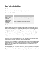
Beer's law
light filter
Light filter
respite
counter
lf_count
Integer
Number of years of respite for a
new seedling from the effects of
the light filter.
Rooting
height
z
Float
The height, in mm, above ground Beer's law
level at which a seedling is rooted. light filter
The absolute
growth
behaviors
Years
released
ylr
Integer
The length of the current release
period, in years.
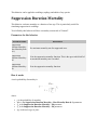
Years
suppressed
yls
Integer
The length of the current
suppression period, in years.
The absolute
growth
behaviors
Integer
A flag for whether a tree has died
and why. Integer of one of the
following: 0 = not dead, 1 =
harvest, 2 = natural causes, 3 =
disease, 4 = fire, 5 = insects, or 6
= storm. This is used by the dead
tree remover behavior to find the
trees it should remove.
Any of the
mortality
behaviors
Integer
An integer value with the damage
level of a storm and how long it
has been damaged. A value of 0
means no damage; a value starting
with 1 means medium damage; a
Storm
value starting with 2 means
damage
complete damage. The digits at
applier
the end count how many years
since the damaging event. For
example, a value of 1005 is a tree
that received medium damage 5
years ago.
Tree bole
volume
calculator
Tree volume
Dead flag
Storm
Damage
Value
dead
stm_dmg
Tree Bole
Volume
Bole Vol
Float
The volume of a tree, in cubic
feet.
Tree
Volume
Float
Volume of the tree, in cubic
Volume
meters.
calculator
Tree
Biomass
Biomass
Float
Biomass of the tree, in metric tons Dimension
(Mg).
analysis
Tree Age
Tree Age
Integer
Age of the tree, in years.
Tree age
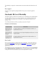
Snag Decay
SnagDecayClass
Class
Integer
Snag decay class.
Snag Decay
Class
Dynamics
New Break
NewBreakHeight
Height
Float
Snag break height, if the break
occurred this timestep. -1 if the
snag is unbroken.
Snag Decay
Class
Dynamics
Snag break height, if the break
occurred in a previous timestep. 1 if the snag is unbroken.
Snag Decay
Class
Dynamics
Snag Old
Break
Height
SnagOldBreakHeight Float
Fall
Fall
Pre-harvest
PreHarvGr
growth
Whether a tree that has died this
Snag Decay
Boolean timestep has fallen (true), or
Class
remains standing as a snag (false). Dynamics
Float
Growth prior to the last harvest.
Lagged post
harvest
growth
Last
stochastic
autocorr
Float
The previous year's stochastic
growth factor.
Michaelis
Menton with
negative
growth height only
Years
Infested
YearsInfested
Integer
The number of years that a tree
has been infested with insects.
Insect
Infestation
Vigorous
vigorous
Boolean
Whether a tree is vigorous or not
(true or false).
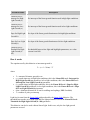
Tree Quality
Vigor
Classifier
sawlog
Whether a tree is sawlog quality
Boolean
or not (true or false).
Tree Quality
Vigor
Classifier
Integer
Tree Quality
Vigor
Classifier
Sawlog
Tree class
treeclass
What is a behavior?
Tree class number, 1-6.
Behaviors are the active part of a SORTIE simulation. Nothing in the model is pre-defined,
default, or automatic. Everything that happens is done by a behavior, and all behaviors are under
user control.
Behaviors fall into two categories. The first category is behaviors that act on trees and roughly
correspond to biological and environmental processes. These behaviors calculate how much
individual trees grow, select trees that will die, distribute seeds, and perform other similar jobs.
The second category is behaviors that perform helper functions for the simulation itself. These
behaviors do things like measure and calculate forest metrics and write output.
Each behavior has a clearly defined action. Each behavior in a run performs its action once per
timestep in a pre-defined order.
Relationship of behaviors to trees and grids
Trees and grids are the state data of SORTIE. Behaviors act on this data to change it and evolve
the model state.
Behaviors are assigned to specific data, and may not act outside this scope.
SORTIE directly manages all the state data needed for a given simulation and automatically
ensures the creation of any data that a behavior is assigned to work on. Users can adjust the
initial conditions of all state data at the beginning of the simulation.
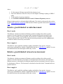
Choosing behaviors for a run
Setting up behaviors is the most important step in creating a new simulation. To choose which
behaviors to include in the run and how to apply them, use the Model flow window.
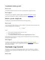
There are a few general guidelines for choosing a set of behaviors from scratch.
Start with the trees
Behaviors that act on trees are assigned to trees based on species and life history stage (otherwise
referred to as tree type). Move through the tree life cycle for each species and pick behaviors for
growth, mortality, and reproduction. There may not be a behavior that does exactly what you
want, but with the creative use of behavior parameters, you may be able to achieve the same
effect. For instance, there may be a parameter that when assigned a particular value cancels out a
function term you don't need, or a set of parameter values that can cause a function to mimic
another function shape.
Carefully check the behavior assignments to particular trees. Behaviors often have some rules
about how they can be applied, but these tend to be limited in the interests of maximum
flexibility. The model doesn't try to second-guess what you are doing beyond making sure the
simulation can run as described. Make sure that you applied a complete set of lifecycle behaviors
to each species and life history stage.
Check the dependencies
Many behaviors rely on the work of other behaviors. Check the documentation for the set of
behaviors you have so far to see if you need to add others. For instance, if you have a behavior
that calculates growth as a function of light level, you will need to add a behavior to calculate the
light level. Each behavior's documentation will give you all dependency requirements.
Add analysis and output
Forest metrics and output are handled by behaviors just like everything else in SORTIE. Basic
metrics like stem density and basal area are handled directly by the output behavior. You can add
additional behaviors (called analysis behaviors) to calculate extra metrics like biomass or tree
spatial distribution indexes.
Output is one of a set of behaviors that uses a separate interface for setup - in this case, the
Output setup window.
It is generally a good idea to finish setting up a parameter file at this point and to run it. There is
generally troubleshooting to be done on the basic lifecycle behaviors and the fewer behaviors
that are in a run, the easier it is to identify and fix problems.
Add external events
If you have behaviors you would like to use beyond the basic tree lifecycle, add them at this
point. These include things like disturbance events and climate change.
Check behavior order
The parameter file specifies which behaviors to include in the simulation, and in which order
they should be run. Theoretically it is possible to put behaviors in any order, but of course, most
simulations constructed that way would not make sense. When you structure a run, the behaviors
are placed in functional groups. To prevent nonsensical simulations, you cannot move a behavior
outside of its functional group in the overall run order; however, you can re-order behaviors
within the functional groups. Sometimes this will have an effect on the overall simulation
outcome, and sometimes it won't. Refer to the documentation for individual behaviors and
functional groups to learn how run order might affect a behavior.
Setting up behaviors: parameters
Almost all behaviors need values and settings from the user to function. These are called the
behavior parameters.
Once you have established the set of behaviors for your run, you will need to provide values for
all parameters for those behaviors. To edit the behavior parameters, use the "Edit-> Parameters"
menu option. You may want to work with one set of parameters at a time when you are first
entering them, because the window will validate your entries before accepting them and it will be
easier troubleshoot one section at a time.
When editing the parameters, if you are not sure what a parameter is or what value you should
enter, you can check the parameters page for that behavior functional group. It lists all
parameters for all behaviors in that group in alphabetical order with a short description of each,
and tells you what behavior they belong to.
Once the parameters are entered, you can view them all at once and save a copy of a text version
as a record.
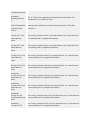
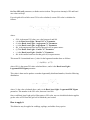
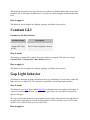
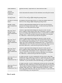
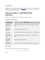
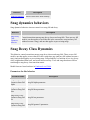
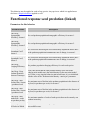
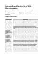
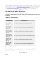
State change behaviors
State change behaviors act on the basic properties of the virtual plot being modeled.
Behavior
Description
Precipitation
Climate
Change
behavior
Changes the value of the Mean Annual Precipitation parameter of the SORTIE
plot.
Temperature
Climate
Change
behavior
Changes the value of the Mean Annual Temperature parameter of the SORTIE
plot.
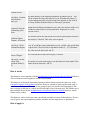
Precipitation Climate Change
This behavior changes the value of the Mean Annual Precipitation parameter of the SORTIE
plot. This can be used to simulate the effects of climate change. If the run does not have a
behavior that uses precipitation, this will have no effect.
Parameters for this behavior
Parameter name
Description
Precipitation Change
-B
"B" in the function for varying precipitation through time.
Precipitation Change
-C
"C" in the function for varying precipitation through time.
Precipitation Change
- Precip Lower
Bound
The lower bound for allowed precipitation values.
Precipitation Change
- Precip Upper
Bound
The upper bound for allowed precipitation values.
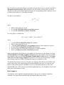
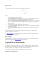
How it works
The value for plot precipitation is a function of time elapsed since the start of the run, as follows:
P = P1 + B * t C
where:





P is the mean annual precipitation, in mm, at time t
P1 is the mean annual precipitation value at the start of the run, as assigned in the Plot
parameters
B is the Precipitation Change - B parameter
C is the Precipitation Change - C parameter
t is the time elapsed, in years, since the start of the run
This value is then given to the Plot object which makes it available to other behaviors in the run.
You can set bounds on the possible precipitation values using the Precipitation Change Precip Lower Bound and Precipitation Change - Precip Upper Bound parameters. Values are
not allowed to go outside these limits.
How to apply it
Add this behavior to the run. You can use it alone or in addition to the Temperature Climate
Change behavior. You do not need to assign this behavior to trees.
Temperature Climate Change
This behavior changes the value of the Mean Annual Temperature parameter of the SORTIE
plot. This can be used to simulate the effects of climate change. If the run does not have a
behavior that uses temperature, this will have no effect.
Parameters for this behavior
Parameter name
Description
Temperature Change
-B
"B" in the function for varying temperature through time.
Temperature Change
-C
"C" in the function for varying temperature through time.
Temperature Change
- Temp Lower
Bound
The lower bound for allowed temperature values.
Temperature Change
The upper bound for allowed temperature values.
- Temp Upper Bound
How it works
The value for plot temperature is a function of time elapsed since the start of the run, as follows:
T = T 1 + B * tC
where:





T is the mean annual temperature, in degrees C, at time t
T1 is the mean annual temperature value at the start of the run, as assigned in the Plot
parameters
B is the Temperature Change - B parameter
C is the Temperature Change - C parameter
t is the time elapsed, in years, since the start of the run
This value is then given to the Plot object which makes it available to other behaviors in the run.
You can set bounds on the possible temperature values using the Temperature Change - Temp
Lower Bound and Temperature Change - Temp Upper Bound parameters. Values are not
allowed to go outside these limits.
How to apply it
Add this behavior to the run. You can use it alone or in addition to the Precipitation Climate
Change behavior. You do not need to assign this behavior to trees.
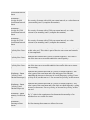
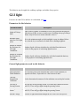
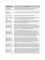
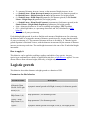
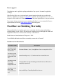
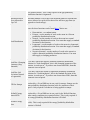
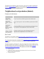
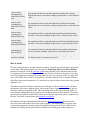
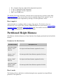
Disturbance behaviors
Disturbance behaviors simulate different kinds of forest disruption. These behaviors cause tree
damage and death due to a variety of processes.
Behavior
Description
Competition
Harvest
Performs harvests in a way that preferentially removes the most competitive
individuals in a plot.
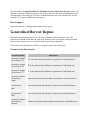
Generalized
Harvest
Regime
The behavior itself decides when harvests will occur and how much to cut based
on total plot adult biomass, then chooses trees to cut with the help of a preference
algorithm.
Harvest
Implements complex silvicultural treatments.
Harvest
interface
Allows SORTIE to work directly with an external harvesting program.
Insect
Infestation
Simulates an insect outbreak by choosing and marking infested trees.
Episodic
mortality
Allows you to replicate tree-killing events with the same level of control you
have when defining Harvest events.
Random
browse
Simulates random browsing from herbivores.
Storm
disturbance
Simulates the effects of wind damage from storms.
Storm
damage
applier
Decides which trees are damaged when a storm has occurred and how badly.
Storm
Kills trees damaged in storms.
damage killer
Storm direct
killer
Kills trees based on storm severity, without an intervening damage step.
Selection
harvest
Allows you to specify target basal areas for a tree population as a method of
harvest input, instead of designing specific harvest events.
Windstorm
Kills trees due to storm events.
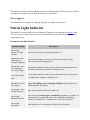
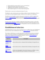
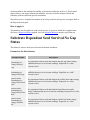
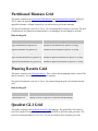
Competition Harvest
Competition Harvest performs harvests in a way that preferentially removes the most
competitive individuals in a plot. It also decides when and how much to harvest based on criteria
you give it.
Trees removed by this behavior will have a mortality reason code of "harvest".
Parameters for this behavior
Parameter name
Description
Competition
Harvest: Amount of
Harvest Per Species
(0 - 1)
Trees to harvest can be treated as a common pool where species identity
is not a factor in selecting trees for harvest. In this case, all values should
be set to 1.0. Otherwise, species can be harvested at a fixed proportion.
In this case, set the proportion to harvest for each species as a value
between 0 and 1, with all values adding up to 1.
Competition
Harvest: Amount to
Harvest
Amount to harvest, depending on the harvest type. If this is a fixed
interval harvest (the value in Competition Harvest: Harvest Type is set
to "Fixed Interval"), this is the basal area of the plot after harvesting, in
m2/ha; if this is a fixed basal area threshold harvest with a fixed amount
to cut ("Fixed BA Amt"), this is the amount of basal area to cut, in m2/ha;
if this is a fixed basal area threshold harvest with proportion of total to
cut ("Fixed BA %"), this is the proportion of the total plot's basal area to
cut between 0 and 1.
Competition
Harvest: C
The slope of the curve "C" of the competitive effect of a target on a
neighbor of each species.
Competition
Harvest: D
The steepness of the curve "D" of the competitive effect of a target on a
neighbor of each species.
Competition
Harvest: DBH Effect
of Targets (alpha)
Exponent controlling the effect of a target's DBH on neighbors.
Competition
Harvest: Distance
Effect of Targets
(beta)
Exponent controlling the effect of distance between target and neighbors.
Competition
Harvest: Filename
for List of Harvested
Trees
Optional. If there is a value in this field, the Competition Harvest
behavior will write a tab-delimited text file of this name with all the trees
cut during the run. In batch runs this will get overwritten and only
contain the last run's list.
Competition
Harvest: Fixed BA
Harvest Threshold
(m2/ha)
For fixed basal area threshold harvests (the value in Competition
Harvest: Harvest Type is set to either "Fixed BA %" or "Fixed BA
Amt"), this is the amount of basal area that the plot must have before a
harvest occurs. This value is ignored if the harvest type is "Fixed
Interval".
Competition
Harvest: Fixed
Interval Harvest
Interval (yr)
For fixed basal area threshold harvests (the value in Competition
Harvest: Harvest Type is set to "Fixed Interval"), this is the number of
years between harvests. This value is ignored if the harvest type is "Fixed
BA %" or "Fixed BA Amt".
Competition
Harvest: Harvest
Type
The type of harvest to perform. "Fixed BA %" means that there is a
harvest every time the plot reaches a fixed basal area threshold, and the
amount cut is a proportion of the total basal area; "Fixed BA Amt" means
that there is a harvest every time the plot reaches a fixed basal area
threshold, and the amount to cut is a fixed amount of basal area; "Fixed
Interval" means that there is a harvest every X years, with the plot being
harvested until it is cut back to a certain amount of basal area.
Competition
Harvest: Minimum
DBH to Harvest
The minimum DBH, in cm, of trees that can be harvested.
Competition
Harvest: Min Years
Between Fixed BA
Harvests
For fixed basal area threshold harvests (the value in Competition
Harvest: Harvest Type is set to either "Fixed BA %" or "Fixed BA
Amt"), this is the minimum number of years that must pass between
harvests, even if the plot basal area is over the harvesting threshold. This
value is ignored if the harvest type is "Fixed Interval".
Competition
Harvest: Maximum
DBH to Harvest
The maximum DBH, in cm, of trees that can be harvested.
Competition
Harvest: Max Radius
of Competitive
Effects (m)
The maximum radius in meters at which a target tree of that species
competitively affects other trees.
Competition
Harvest: Species i
Target Lambda
The competitive effect of targets of Species i on neighbors of every other
species.
Competition
Harvest: Size
Sensitivity (gamma)
The effect of a neighbor tree's size on its sensitivity to competition.
Competition
The value by which target DBHs are divided when calculating
Harvest: Target DBH competitive effects. This can be used to make units adjustments.
Divisor
Gen Harvest
Acceptable
Deviation From Cut
Target
The amount by which it is acceptable to deviate from the harvest target
basal area removal without triggering a second harvest pass. Expressed
as a proportion of the target basal area, between 0 and 1.
How it works
Competition Harvest performs harvests when specific conditions are met in the plot. The amount
harvested is also based on conditions in the plot. There are three ways to specify the timing and
amount of harvesting. The desired method is set in the Competition Harvest: Harvest Type
parameter. The harvest types are:



Fixed basal area threshold, cutting a specific amount of basal area. (Set the harvest type
parameter to "Fixed BA Amt".) A harvest occurs whenever the plot's basal area exceeds a
certain threshold, set in the Competition Harvest: Fixed BA Harvest Threshold
(m2/ha) parameter. The same amount of basal area is harvested every time, set in the
Competition Harvest: Amount to Harvest parameter. To make sure that harvests do
not happen too frequently, set a minimum interval between harvests in the Competition
Harvest: Min Years Between Fixed BA Harvests parameter.
Fixed basal area threshold, cutting a proportion of the plot basal area. (Set the harvest
type parameter to "Fixed BA %".) This is the same as the first harvest type, except the
amount to harvest is different. This harvest removes a set proportion of the plot's basal
area. Set this proportion (between 0 and 1) in the Competition Harvest: Amount to
Harvest parameter.
Fixed interval, cutting plots back to a basal area threshold. Harvests occur at a fixed
interval, set in the Competition Harvest: Fixed Interval Harvest Interval (yr)
parameter. The first timestep will have a harvest. Harvests remove trees until the plot
reaches a specific amount of basal area, set in the Competition Harvest: Amount to
Harvest parameter.
Competition Harvest uses these criteria to determine when and how much to cut. Harvests occur
over the the entire plot area.
During a harvest, Competition Harvest calculates how much basal area it needs to cut. It can
select trees without regard to species, or it can remove trees in a set ratio. Species ratio is set in
the Competition Harvest: Amount of Harvest Per Species (0 - 1) parameter. If all values are
set to 1, this means that species identity is ignored when selecting individuals for harvesting.
Otherwise, the species are cut in the proportions entered. The values should add up to one. For
example, if Species 1 is set to 0.25 and Species 2 is 0.75, then Competition Harvest will try to
make 25% of the basal area removed come from Species 1 individuals and 75% come from
Species 2. Of course, there are trade-offs between removing the most competitive individuals
and making sure specific species targets are met.
When selecting trees for harvesting, Competition Harvest removes the individuals that have the
greatest competitive effects on their neighbors. The neighbors of an individual are all sapling and
adult trees within the radius specified in the Competition Harvest: Max Radius of
Competitive Effects (m) parameter. (Seedlings, snags, and dead trees never count as neighbors.)
The competitive effect (COE) of tree i on the N neighbors surrounding it is:
where:









C is the Competition Harvest: C parameter for the species of neighbor j
D is the Competition Harvest: D parameter for the species of neighbor j
α is the Competition Harvest: DBH Effect of Targets (alpha) parameter for the species
of neighbor j
β is the Competition Harvest: Distance Effect of Targets (beta) parameter for the
species of neighbor j
γ is the Competition Harvest: Size Sensitivity (gamma) parameter for the species of
neighbor j
DBHj is the DBH, in cm, of neighbor j
λ is the Competition Harvest: Species i Target Lambda parameter for the species of
neighbor j, where Species i is the target's species
DBHi is the DBH, in cm, of target i
dist is the distance between target and neighbor, in meters
Competition Harvest removes the tree with the highest COE value in the plot, then updates the
COE of each tree in the vicinity so that the removed tree is no longer a neighbor. This process is
repeated until the harvest cut target has been reached. If removing a tree will cause the harvest to
overshoot its cutting target, a random number is compared to the amount of overshoot to
determine if the tree will be removed, then harvest ends. If species are to be cut in a certain
proportion, then separate cut targets are maintained for each species. If the highest COE
individual is of a species whose cut target has been reached, it is not cut and Harvest
Competition searches for the highest COE individuals of other species.
Only trees to which you have applied the Competition Harvest behavior are considered for
harvesting. You can only apply the behavior to saplings and adults. You can specify a size range
to cut using the Competition Harvest: Minimum DBH to Harvest and Competition Harvest:
Maximum DBH to Harvest parameters.
The Competition Harvest behavior stores how much it actually cut each timestep in the
Competition Harvest Results grid. Additionally (and optionally), you can give the behavior a
filename with the Competition Harvest: Filename for List of Harvested Trees parameter. If a
filename is present, Competition Harvest will write to this file a list of the individuals harvested
each timestep for the entire run. The file is a tab-delimited text file, with a header line, and five
columns: X, Y, Species, DBH, and Timestep cut.
How to apply it
Apply this behavior to saplings and/or adults of any species.
Generalized Harvest Regime
This behavior can perform harvest very flexibly, depending on the parameters used. The
behavior itself decides when harvests will occur and how much to cut based on total plot adult
biomass, then chooses trees to cut with the help of a preference algorithm.
Trees removed by this behavior will have a mortality reason code of "harvest".
Parameters for this behavior
Parameter name
Description
Gen Harvest Regime
Cut Preference "A"
"A" in the function that calculates cut preference of individual trees.
Gen Harvest Regime
Cut Preference "B"
"B" in the function that calculates cut preference of individual trees.
Gen Harvest Regime
Cut Preference "C"
"C" in the function that calculates cut preference of individual trees.
Gen Harvest Regime
Cut Preference
"Alpha"
Alpha in the function that calculates cut preference of individual trees.
Gen Harvest Regime
Cut Preference
"Beta"
Beta in the function that calculates cut preference of individual trees.
Gen Harvest Regime
Cut Preference
"Beta"
Beta in the function that calculates cut preference of individual trees.
Gen Harvest Regime
Cut Preference
"Gamma"
Gamma in the function that calculates cut preference of individual trees.
Gen Harvest Regime
Cut Preference "Mu"
Mu in the function that calculates cut preference of individual trees.
Gen Harvest Regime
Gamma Scale
Parameter
Scale parameter for the gamma probability distribution function.
Gen Harvest Regime
Harvest Probability
"A"
"A" term in the function that determines the probability that the plot will
be harvested this time step.
Gen Harvest Regime
Harvest Probability
"B"
"B" term in the function that determines the probability that the plot will
be harvested this time step.
Gen Harvest Regime
Harvest Probability
"M"
"M" term in the function that determines the probability that the plot will
be harvested this time step.
Gen Harvest Regime
Remove Amount
"Alpha"
"Alpha" term in the function that determines percentage of adult basal
area to be removed from the plot.
Gen Harvest Regime
Remove Amount
"Beta"
"Beta" term in the function that determines percentage of adult basal area
to be removed from the plot.
Gen Harvest Regime
Remove Amount
"Mu"
"Mu" term in the function that determines percentage of adult basal area
to be removed from the plot.
How it works
The behavior begins the time step by deciding whether or not a harvest will occur. The
probability of harvest is a function of total plot adult biomass, as follows:
where:





P is the probability that the plot will be harvested this time step
Bio is the total plot adult biomass, in Mg/ha, as calculated by the Dimension analysis
behavior
a is the Gen Harvest Regime Harvest Probability "A" parameter
m is the Gen Harvest Regime Harvest Probability "M" parameter
b is the Gen Harvest Regime Harvest Probability "B" parameter
A random number is compared to this probability to decide whether or not harvest will occur.
The frequency of harvest in previous time steps is not take into account.
If harvest is to occur, the percentage of adult basal area to remove is calculated as follows:
where:





BAR is the mean percent of total plot adult basal area to remove, between 0 and 100
Bio is the total plot adult biomass, in Mg/ha, as calculated by the Dimension analysis
behavior
α is the Gen Harvest Regime Remove Amount "Alpha" parameter
β is the Gen Harvest Regime Remove Amount "Beta" parameter
μ is the Gen Harvest Regime Remove Amount "Mu" parameter
Note that the BAR is the mean removal rate. This value is used, along with the Gen Harvest
Regime Gamma Scale Parameter, in a draw on the gamma distribution in order to get the
actual target removal rate.
The plot biomass in the equations above is the total adult biomass for all species. All species
must participate in harvest, and only adults are counted and cut.
Once a basal area removal target has been established, the individuals to cut must be selected. A
preference function determines the probability that an individual will be cut, as follows:
where:







Pi is the probability that individual i will be cut
α i is the Gen Harvest Regime Cut Preference "Alpha" parameter for the species of
individual i
β i is the Gen Harvest Regime Cut Preference "Beta" parameter for the species of
individual i
γ i is the Gen Harvest Regime Cut Preference "Gamma" parameter for the species of
individual i
μ i is the Gen Harvest Regime Cut Preference "Mu" parameter for the species of
individual i
BAR is the percent of total adult basal area to remove, between 0 and 100
DBH is the individual's DBH
The term σ is:
σ = a + b * BAR c
where:




a is the Gen Harvest Regime Cut Preference "A" parameter
b is the Gen Harvest Regime Cut Preference "B" parameter
c is the Gen Harvest Regime Cut Preference "C" parameter
BAR is the percent of total adult basal area to remove, between 0 and 100
An individual's probability of removal is compared with a random number to determine if that
individual is cut.
The preference function takes into account the target basal area removal rate of the plot.
However, the function shape does not necessarily produce a mean removal probability equal to
that of the target removal rate, particularly near 0 and 100. If you wish, the behavior can refine
the probabilities on a second pass to get closer to the target. You can set a tolerance using the
Gen Harvest Acceptable Deviation From Cut Target parameter. This is expressed as a
proportion of the removal rate, between 0 and 1. So a value of 0.1 allows first-pass acceptable
deviation of 10 percent from the target. If the actual removal rate falls outside this limit, the
function adjusts all preferences by a correction factor and re-evaluates individual cut decisions.
No more than two passes will be made, even if the second pass does not achieve a removal rate
within the tolerance. Setting a high tolerance such that a second pass is not often needed
eliminates a lot of calculations and will allow a run to be faster.
How to apply it
Apply this behavior to the adults of all species. You must also apply the Dimension analysis
behavior to the same trees.
Harvest
Trees removed by this behavior will have a mortality reason code of "harvest".
Parameters for this behavior
This behavior does not have its parameters entered through the Parameters Window. Set up these
behaviors using the Edit Episodic Events Window.
How it works
SORTIE can implement complex silvicultural treatments. Harvest events are defined by species,
timestep, amount to remove, type of cut, and area of the plot. You can define as many harvest
events as you wish. For information on planting new seedlings, see the Planting behaviors topic.
There are three types of harvest: gap cut, partial cut, and clear cut. The primary function of
entering the harvest type is to control substrate composition after the harvest occurs. In a partial
cut harvest, though, you have more flexibility in choosing which trees are cut. You can define up
to four size classes, and specify the amount of trees to remove in one of four ways: as a
percentage of total basal area, as an absolute amount of basal area, as a percentage of total tree
density, or as an absolute amount of tree density.
The Harvest behavior selects the trees to remove in the same way for all three harvest types.
When it is determining which trees to remove, it starts by finding the largest tree in the area of
the plot affected by the harvest. It works its way through the trees from largest to smallest,
assessing whether to cut each one until it either runs out of trees or reaches its cut target. This
process preferentially removes the largest trees in each size range, unless the harvest is a
percentage of density cut, in which case all trees in the target size ranges have an equal
probability of being cut. If Harvest is cutting a percentage of basal area or an absolute amount of
basal area, it will only cut a tree if its basal area will not cause the total to be more than the
target. This means that, for basal-area-defined cuts, the Harvest behavior may skip some bigger
trees and cut smaller ones in order to more exactly cut its target. Each species is cut separately.
So, a request to remove 20% of three species will remove 20% of each of them, no matter what
their relative proportions to each other.
Trees can be prioritized for harvest. You can choose a tree data member and a range of values for
that data member. For instance, you could prioritize trees with growth values between 5 and 10.
Trees meeting a priority are cut first.
You can set up to three priorities. All trees meeting the first priority are cut first, then all trees
meeting the second priority, then all meeting the third, then all other trees. Cutting stops when
the target removal amount has been met. DBH ranges are honored. If there is a priority tree
outside the cut DBH ranges, it will not be cut under any circumstances. The exception to priority
ordering is in the case of a basal area cut target. If a priority tree would cause too much basal
area to be removed, a smaller non-priority tree may be cut instead to more precisely reach the
target. Priorities may not be applied to percent of density cuts, because these cuts are stochastic
in nature so prioritization is meaningless. You can prioritize by the same data member more than
once; for instance, first cut trees with growth between 5 and 10, then with growth between 0 and
5.
Although seedlings are not properly harvested, a harvest can kill them just the same. You can
specify the proportion of seedlings that are killed within the harvest area for each species. The
seedlings of a species can be killed even if that species is not being harvested. Seedlings in the
harvest area are randomly chosen to die based on the mortality rate for their species. They are
given "harvest" as a mortality reason.
Trees that are harvested are removed immediately. When light is calculated for that timestep,
gaps opened up by the harvest will be visible. If there are behaviors which apply to stumps, a
stump is created for each logged tree. Otherwise, the tree completely disappears.
The actual amount of tree harvest may not be exactly what was specified, since the Harvest
behavior can't remove part of a tree to get the numbers right. The behavior stores how much it
actually cut each timestep in the Harvest Results grid. To optimize the accuracy of the Harvest
behavior, use larger cut ranges and high proportions of the plot area to make sure there is a big
pool of trees to choose from.
How to apply it
To add harvesting to a SORTIE run, use the Edit Episodic Events Window.
Harvest interface
The harvesting interface allows SORTIE to work directly with another program. SORTIE tells
the other program what trees are eligible for harvesting, and the other program replies with its
choices. This lets users write code for harvesting without having to modify SORTIE itself.
Warning - this link between SORTIE and another program is inefficient. It may be very slow
when there are large numbers of trees. It is for convenience, not speed.
Trees removed by this behavior will have a mortality reason code of "harvest".
How it works
You set up the Harvest Interface behavior using the Edit->Harvest Interface window. Parameters
in this documentation are defined by their names on that screen.
You either create or find a separate program (an executable) that reads a text file of trees, makes
decisions about which to kill, then writes those trees to kill to another text file. You tell SORTIE
where to find this executable using Path and filename of the executable on the Edit Harvest
Interface window.
Each harvest timestep, SORTIE writes a text file with a list of trees eligible for harvest. The trees
in the list are those to which the Harvest Interface behavior is applied. You choose which trees
those are in Behavior currently assigned to on the Edit Harvest Interface window. Once the file
is written, SORTIE then launches your executable. Your executable writes a file in response with
the list of trees it wishes SORTIE to kill.
Trees that are cut are treated exactly like those in SORTIE harvest. That is, they disappear
completely and do not become snags. See the documentation on Harvest for more details. The
cut details for each timestep are written to the Harvest Results grid. (Warning - if you put both
the Harvest and Harvest Interface behavior in the same run, they will overwrite each other's
results in the grid.)
Because the process can be slow, you can set harvests to occur less often than every timestep. To
do this, use How often to harvest, in years on the Edit Harvest Interface window.
Optionally, you can also add new tree data members that are controlled by the executable. The
executable can write a file with a list of trees to update, and the new values for those variables
for each tree.
File formats
Each harvesting timestep, SORTIE begins by writing a file of all trees eligible for harvest. You
give SORTIE the path and name of that file in Tree file that SORTIE will write on the Edit
Harvest Interface window. SORTIE does not care what the filename nor file extension is. The
file is tab-delimited text. It has the following format:
Line 1, two columns: Current timestep, total number of timesteps
Line 2, column names, 6+n columns: "X", "Y", "Species", "Type", "Diam", "Height", [...]
Subsequent lines, 6+n columns, one line per tree: X, Y, species number, type number,
DBH/diam10, height, [...].
Species is given as a number from 0 to x - 1, where x is the number of species. The number
counts the species in the order in which they are listed in the parameter file, which is the same as
the order they are listed in the Edit Species window.
Type is given as a number as well. The type numbers are:
1.
2.
3.
4.
5.
Seedling
Sapling
Adult
Stump
Snag
Stumps are not available for harvesting.
The "Diam" value is diameter at 10 cm if the tree type is seedling, and DBH in all other cases.
Both of these values are in cm.
The "Height" value is the height of the tree in meters.
The [...] represents additional columns that you can ask SORTIE to include. You set this up
using the File columns section of the Edit Harvest Interface window. You can choose any other
tree data member that applies to all of the kinds of trees to which the harvest interface is applied,
including new ones that you add. The list of tree data members depends on the other behaviors in
the run. The column header matches the internal SORTIE name of the data member (which is
what is displayed to you when you choose new data members). You cannot change the first six
default columns.
The executable writes a file in response with the trees that it wishes to harvest (Tree harvest file
that the executable will write on the Edit Harvest Interface window). If you have set up new
tree data members, the executable also writes a second file with a list of live trees to update
(Tree update file that the executable will write on the Edit Harvest Interface window). All
trees in both of these files must come from the tree list that SORTIE wrote for that timestep. No
tree may appear in both files.
The file format of the user response files is identical to that of the SORTIE file, with the same
columns in the same order.
Each harvest timestep, all these files are overwritten.
If there are no trees eligible for harvesting, SORTIE still writes a file with only the first two
header lines (no individual tree lines). It expects the executable to do the same if it does not want
trees harvested or updated.
Adding new variables
You can request that SORTIE create new data members under the executable's control for the
trees to which this behavior applies. Set this up in the New tree data members to add section of
the Edit Harvest Interface window. You can create as many as you want. You can give them any
name up to 9 characters long. They each hold a float value. The values are uninitialized in newly
created trees.
If you want the new data members to be written to the file that SORTIE writes, make sure you
put them in the list of file columns.
If new data members have been created, SORTIE expects the executable, each time it is called,
to write a file with the list of trees it wishes to update, and the new values for these data
members. You can only make changes to the new data members that you create. You cannot
change any other attribute of a tree.
The user executable
The user executable launches, runs, and quits once per harvest timestep. SORTIE waits for it to
finish before resuming. This means it must do any necessary initialization and setup each harvest
timestep.
The executable can be written in any language, and can do anything it wishes. The only two
requirements is that it be a standalone executable, and that it produce the file of trees to harvest
that SORTIE expects.
The executable should be prepared for the condition that there are no trees in the file SORTIE
writes, and should write empty files if it doesn't want any trees harvested or updated.
SORTIE's behavior cannot be guaranteed in the event of a crash in the user executable.
The executable probably has its own input data for setup. If it takes arguments during launch,
you can give SORTIE a string to pass to the executable in Arguments to pass to the executable
on the Edit Harvest Interface window.
SORTIE provides a convenience feature for those executables that read setup parameters from a
file. You may wish to set up a SORTIE batch run where your executable uses different
parameters for each run. You can give SORTIE a file of all the parameters for the entire batch in
a text file, and for each run, it will separate out that run's parameters and write them to a file for
your executable. The parameters for a single run must be on a single line of the entire batch file,
and will be written to a one-line file for the individual run. Specify the entire-batch parameters
file in Parameters file for batch run, and the single-run file in Single-run parameters file for
batch run on the Edit Harvest Interface window.
For example, suppose there is an executable that takes three parameters. It reads these parameters
from a one-line file named "par.txt", like this:
par1 par2 par3
You can set up a batch of three runs, then set up all the parameters in a single file, like this:
par1_1 par2_1 par3_1
par1_2 par2_2 par3_2
par1_3 par2_3 par3_3
You give SORTIE this file, and tell it to write "par.txt" for each run. The first run in the batch,
SORTIE will write the first line to "par.txt"; the second run in the batch, it will write the second
line to "par.txt", etc.
Tips:
If you are having trouble with SORTIE not finding your code's output file, try explicitly writing
out directories in your code (i.e. "C:\sortie\file.txt" instead of just "file.txt").
How to apply it
It is easiest if you add the harvest interface after the rest of your parameter file is complete, so
that you have full access to data members. Open Edit->Harvest Interface and complete the setup.
This adds the harvest interface behavior to your run. To remove it, use the Model flow window.
Insect Infestation
This behavior simulates an insect outbreak. It chooses and marks affected trees, allowing other
behaviors to make use of this information. The number of affected trees is a function of time
since infestation began. The infestation has no spatial pattern.
This behavior only chooses trees for infestation. It does not kill them or alter their dynamics in
any way. Other behaviors may take advantage of the infestation status information of trees.
Parameters for this behavior
Parameter name
Description
Insect Infestation
First Timestep
The timestep that an insect infestation begins.
Insect Infestation
Initial Rate
The rate of infestation on the first timestep of the outbreak.
Insect Infestation
Max Rate
The maximum rate of infestation.
Insect Infestation
Min DBH
The minimum DBH of trees that can become infested.
Insect Infestation X0
The time at which 0.5 of the maximum infestation rate occurs.
Insect Infestation Xb
Parameter controlling the steepness of the rise of the infestation rate.
How it works
The proportion of trees of a particular species infested as a function of time is as follows:
where:





P is the proportion of the eligible tree population infested.
I is the Insect Infestation Initial Rate parameter, as a value between 0 and 1. This is the
function intercept, or the infestation rate at the first timestep of infestation.
Max is the Insect Infestation Max Rate parameter, as a value between 0 and 1. This is
the maximum infestation rate that will occur regardless of how long the infestation lasts.
T is the time, in years, since the start of the infestation.
X0 is the Insect Infestation X0 parameter. This is the time at which half of the maximum
infestation rate is reached.

Xb is the Insect Infestation Xb parameter. This controls the steepness of the rise of the
curve.
You choose when an infestation begins with the Insect Infestation First Timestep parameter.
The only way that an infestation ends is if there are no more infested trees in the plot.
You can set a minimum DBH of infestation, using the Insect Infestation Min DBH parameter.
The proportion of trees infested at time T does not depend on additions to or subtractions from
the pool of eligible trees. Each timestep, the number of infested trees of each species is counted
and additional trees are randomly selected for new infestation until approximately the right
number are infested. If for some reason there are more trees infested than there should be at that
time, no additional trees are infested.
When selecting trees for infestation, the location of the trees is not considered. It is assumed that
all trees have an equal chance of becoming infested no matter where they are in the plot. This
behavior uses a tree data member called "Years Infested" to track which trees are infested and
how long they have been so.
How to apply it
Apply this behavior to saplings and/or adults of any species.
Episodic Mortality
Trees removed by this behavior will have a mortality reason code of "disease".
Parameters for this behavior
This behavior does not have its parameters entered through the Parameters Window. Set up these
behaviors using the Edit Episodic Events Window.
How it works
The Episodic Mortality behavior allows you to replicate tree-killing events with the same level of
control you have when defining Harvest events. A planned mortality episode can simulate
disease, an insect outbreak, fire, or the like. The main difference between Harvest and Episodic
Mortality is that the Episodic Mortality behavior can create snags, or standing dead trees. A large
snag proportion can significantly affect the light and substrate dynamics of a SORTIE run.
Defining a mortality episode is like defining a partial cut harvest. (Mortality episodes have no
automatic impact on substrate dynamics like harvest events do, although the newly dead trees
may be a source of harvest input.) You can define up to four size classes, and specify the amount
of trees to kill in one of four ways: as a percentage of total basal area, as an absolute amount of
basal area, as a percentage of total tree density, or as an absolute amount of tree density.
When the Episodic Mortality behavior is determining which trees to remove, it starts by finding
the largest tree in the area of the plot affected by the mortality episode. It works its way through
the trees from largest to smallest, assessing whether to kill each one until it either runs out of
trees or reaches its cut target. This process preferentially removes the largest trees in each size
range, unless the event is defined by a percentage of density, in which case all trees in the target
size ranges have an equal probability of being killed. If Episodic Mortality is removing a
percentage of basal area or an absolute amount of basal area, it will only kill a tree if its basal
area will not cause the total to be more than the target. This means that, for basal-area-defined
cuts, the behavior may skip some bigger trees and cut smaller ones in order to more exactly cut
its target. Each species is cut separately. So, a request to remove 20% of three species will
remove 20% of each of them, no matter what their relative proportions to each other.
Seedlings can also be killed as part of a planned mortality episode. You can specify the
proportion of seedlings that are killed within the target area for each species. The seedlings of a
species can be killed even if that species is not otherwise participating in the episode. Seedlings
in the target area are randomly chosen to die based on the mortality rate for their species. They
are given "disease" as a mortality reason.
What happens to dead trees depends on the rest of the run. If there are other behaviors in the run
that deal directly with snags or create them, then the run is "snag-aware". In this case, all adult
trees killed are turned into snags (saplings never become snags). If the run is not "snag-aware",
then the trees are marked as dead. When/if the dead tree remover behavior runs, the dead trees
will be removed at that time. These dead trees are available as input to Substrate.
The actual amount of trees killed may not be exactly what was specified, since the Episodic
Mortality behavior can't remove part of a tree to get the numbers right. The behavior stores how
much it actually cut each timestep in the Mortality Episode Results grid. To optimize the
accuracy of the behavior, use larger kill ranges and high proportions of the plot area to make sure
there is a big pool of trees to choose from.
How to apply it
To define planned mortality episodes, use the Edit Episodic Events Window.
Random browse
This behavior simulates random browsing from herbivores.
Parameters for this behavior
Parameter name
Random Browse Annual Browse
Probability (0-1)
Description
The annual probability, from 0 to 1, of being browsed. This is the mean
probability if the probability is being varied each timestep.
Random Browse Probability PDF
The PDF used to vary the browse probability. "None" means the same
probability is always used. "Normal" means that each timestep, for each
species, a new probability is drawn from a normal distribution.
Random Browse Browse Probability
Standard Deviation
If the probability is being varied each timestep according to a normal
distribution, this is the standard deviation of that distribution. This value
is ignored if the probability is not being varied.
How it works
The trees eligible for browsing are those trees to which this behavior is applied. Each species has
a probability of browse that is the same for all members of that species. Each timestep, for each
eligible tree, a random number is used against its species probability to decide whether the tree is
browsed.
The probability of browse for a species can be constant, or it can vary each timestep. If it is
constant, the probability of browse is always the value in the Random Browse - Annual Browse
Probability (0-1) parameter. If the probability is to vary, a new value is drawn from a random
distribution, using the value in Random Browse - Annual Browse Probability (0-1) parameter
as the mean and the value in Random Browse - Browse Probability Standard Deviation as the
standard deviation. This draw happens once per species per timestep; all individuals of a species
always face the same probability of browse in a given timestep.
If the timestep length is more than one year, the annual probability of browse is turned into a
timestep probability using TP = 1 - (1 - AP)N, where TP is the timestep probability of browse,
AP is the annual probability, and N is the length of a timestep, in years.
Trees that are chosen as browsed are marked as browsed. This behavior does nothing else to
them. Other behaviors, such as growth and mortality, may use this information.
How to apply it
Apply this behavior to any species and type of tree.
Storm disturbance
This behavior simulates the effects of wind damage from storms. Its function is to assess whether
or not storms have occurred in the current timestep, and if they have, how much damage they
have caused. This behavior does not actually cause any trees to be damaged; that is the function
of the Storm damage applier behavior.
Parameters for this behavior
Parameter name
Description
How storm damage susceptibility varies across the plot. If "Uniform",
Plot Storm
then all locations in the plot have an equal susceptibility. If "Mapped",
Susceptibility Pattern then a map is used to show the way locations in the plot vary in
susceptibility.
Return Interval for
Severity Storm Class
0 - 0.1
The return interval, in years, of storms of severity 0 - 0.1. Set this to 0 to
turn off storms of this severity.
Return Interval for
Severity Storm Class
0.1 - 0.2
The return interval, in years, of storms of severity 0.1 - 0.2. Set this to 0
to turn off storms of this severity.
Return Interval for
Severity Storm Class
0.2 - 0.3
The return interval, in years, of storms of severity 0.2 - 0.3. Set this to 0
to turn off storms of this severity.
Return Interval for
Severity Storm Class
0.3 - 0.4
The return interval, in years, of storms of severity 0.3 - 0.4. Set this to 0
to turn off storms of this severity.
Return Interval for
Severity Storm Class
0.4 - 0.5
The return interval, in years, of storms of severity 0.4 - 0.5. Set this to 0
to turn off storms of this severity.
Return Interval for
Severity Storm Class
0.5 - 0.6
The return interval, in years, of storms of severity 0.5 - 0.6. Set this to 0
to turn off storms of this severity.
Return Interval for
Severity Storm Class
0.6 - 0.7
The return interval, in years, of storms of severity 0.6 - 0.7. Set this to 0
to turn off storms of this severity.
Return Interval for
Severity Storm Class
0.7 - 0.8
The return interval, in years, of storms of severity 0.7 - 0.8. Set this to 0
to turn off storms of this severity.
Return Interval for
Severity Storm Class
0.8 - 0.9
The return interval, in years, of storms of severity 0.8 - 0.9. Set this to 0
to turn off storms of this severity.
Return Interval for
Severity Storm Class
0.9 - 1.0
The return interval, in years, of storms of severity 0.9 - 1.0. Set this to 0
to turn off storms of this severity.
Standard Deviation
(lognormal or
normal)
If the Storm Damage Application parameter is set to "Stochastic" and
the Stochastic Pattern Damage Distribution is set to either "Normal"
or "Lognormal", this is the standard deviation used when randomizing
storm severity across the plot. This parameter is ignored if the Storm
Damage Application parameter is not set to "Stochastic" and the
Stochastic Pattern Damage Distribution is not set to either "Normal"
or "Lognormal".
Stochastic Pattern
Damage Distribution
If the Storm Damage Application parameter is set to "Stochastic", this
is the probability distribution function to use for randomizing storm
severity across the plot. This parameter is ignored if the Storm Damage
Application parameter is not set to "Stochastic".
Storm Damage
Application
How storm damage is applied to different locations across the plot. If
"Deterministic", the storm's severity is applied equally to all locations. If
"Stochastic", the storm's severity is randomized across the plot according
to your chosen probability distribution function.
Storm - Storm
Cyclicity Sine Curve
d
Parameter that controls the cyclicity of storm frequency. For no cyclicity,
set this value to 0. This value is part of the sine curve term and controls
the sine amplitude.
Storm - Storm
Cyclicity Sine Curve
f
Parameter that controls the cyclicity of storm frequency. This value is
part of the sine curve term and controls the sine frequency.
Storm - Storm
Cyclicity Sine Curve
g
Parameter that controls the cyclicity of storm frequency. This value is
part of the sine curve term and controls where on the sine curve storms
start occurring.
Parameter that controls the trend of cyclicity of storm frequency. This
Storm - Storm
value is part of the trend term and is the intercept of the function
Cyclicity Trend
controlling the increase or decrease of overall frequency cycling. For no
Function Intercept (i) cyclicity at all, set this term to 1. For no trend in cyclicity, set this term to
0.
Storm - Storm
Cyclicity Trend
Function Slope (m)
Parameter that controls the trend of cyclicity of storm frequency. This
value is part of the trend term and is the slope at which frequency cycling
increases or decreases. For no cyclicity, or no trend in cyclicity, set this
term to 0.
How it works
There are two ways storms can occur: randomly according to a storm regime of your choosing,
or scheduled at certain timesteps. Both methods can be used together.
Random storms according to a storm regime
Storm severity is assessed on a scale from 0 (no damage) to 1 (total damage). This interval of
storm severity values is subdivided into ten storm severity classes. You assign each storm
severity class a return interval. The reciprocal of the return interval gives the annual probability
of each type of storm.
The overall frequency of storms can remain constant, or it can change through time. It has been
reported in Goldenburg et al 2001 that storm activity in the North Atlantic cycles along with sea
surface temperature. This behavior can thus change the storm frequency over time, using either a
sinusoidal pattern, a constant linear change, or both together. In the figure below, curve 1 is a
basic sine wave. Curve 2 has a sinusoidal pattern plus an upwards trend.
The actual probability of an individual storm that takes place in a storm regime with a cyclical
frequency is:
P'(Fi) = P(Fi) * ([d * sin( π * (x-g) / (2f) )] + [mx + i])
Note that the new probability is a baseline probability, P(Fi), multiplied by a value that adjusts
the probability according to where the model is at the given time in the frequency cycle. The
frequency cycle multiplier is itself made up of two terms added together. The first term is the
sine curve cycling, and the second term is the overall trend upwards or downwards.
Terms in the equation:





P'(Fi) is this timestep's annual probability of a storm of the ith return interval, adjusted
according to the frequency cyclicity
P(Fi) is the baseline probability of a storm of the ith return interval; that is, the reciprocal
of the values specified in the Return Interval for Severity Storm Class X parameters
x = 4 * t / Sr, where t is the number of years since the run started and Sr is the Storm Sea Surface Temperature Cyclicity Period (Years) parameter
d is the Storm - Storm Cyclicity Sine Curve d parameter, which controls the sine
curve's amplitude
f is the Storm - Storm Cyclicity Sine Curve f parameter, which controls the sine curve's
frequency



g is the Storm - Storm Cyclicity Sine Curve g parameter, which controls where on the
sine curve storms start occurring
m is the Storm - Storm Cyclicity Trend Function Slope (m) parameter
i is the Storm - Storm Cyclicity Trend Function Intercept (i) parameter
To turn off all cyclicity and use constant storm probabilities, set Storm - Storm Cyclicity Sine
Curve d to 0, Storm - Storm Cyclicity Trend Function Slope (m) to 0, and Storm - Storm
Cyclicity Trend Function Intercept (i) to 1. (The other values are unimportant.) To use only
the sine portion with no trend line, set both Storm - Storm Cyclicity Trend Function Slope (m)
and Storm - Storm Cyclicity Trend Function Intercept (i) to 0. To use only the trend portion,
set Storm - Storm Cyclicity Sine Curve d to 0.
To decide whether storms occur, the behavior compares a random number to the annual
probability of each storm severity class. For timesteps that are longer than one year, the behavior
repeats the random number test for each year in the timestep. This process is repeated for each
storm severity class separately. This means that multiple storms can occur in a single timestep,
and if the timestep is longer than one year, there can be multiple storms in the same severity
class.
Scheduled storms
You can also schedule storms to occur at certain timesteps. Use the Edit Scheduled Storms
window to do this. You specify the year (NOT the timestep) you want the storm to occur, and a
minimum and maximum severity for each. The actual storm severity will be a random number
between the maximum and minimum. You can schedule as many as you want, including multiple
storms per timestep. If there is also a storm regime present (non-zero values for the return
intervals), those storms can also occur. The storm regime storms can also happen between
scheduled storms.
If a storm occurs, the behavior calculates the amount of damage that occurs. A storm's damage
index (severity) is randomly chosen within the boundaries of its severity class. The damage is
stored in a grid called Storm Damage. The final output of the behavior is a map of storm damage
(severity) across the plot, as an index between 0 and 1. If multiple storms occur, each storm's
severity is recorded separately.
The way storm damage is calculated depends on two things: the pattern of storm susceptibility
across the plot (entered in the Plot Storm Susceptibility Pattern parameter), and the method of
storm damage application (entered in the Storm Damage Application parameter). Storm
susceptibility is measured on a scale from 0 (not susceptible to damage) to > 1 (highly
susceptible to damage). The pattern of storm susceptibility can be either "Uniform", meaning all
locations within the plot have a susceptibility of 1, or "Mapped", meaning that you will provide a
map with a susceptibility for each location in a grid called Storm Susceptibility. The method of
storm damage application can be either "Deterministic", meaning that each location receives the
storm's severity index, or "Stochastic", meaning that the storm's severity index provides a mean
around which individual location severities are randomized.
There are two possible probability distribution functions for stochastic damage application:
normal and lognormal.
The normal distribution is:
where σ is the function standard deviation. Mean is zero in this equation; the final value is
reached by adding the function result to the mean.
The lognormal distribution is:
where ζ is the function mean and σ is the standard deviation.
Combining these two parameters provides four possibilities for the way a storm's damage is
applied:
1. Mapped Deterministic. The damage index for a location equals the susceptibility of that
location multiplied by the storm's severity index.
2. Mapped Stochastic. The storm severity for each location is determined by performing a
random draw on a probability distribution function, with the overall storm severity
providing the function mean. Each location's severity is multiplied by its susceptibility to
arrive at the final storm damage index for that location.
3. Uniform Deterministic. All plot locations are directly assigned the storm's severity index.
4. Uniform Stochastic. The storm damage index for each location is determined by
performing a random draw on a probability distribution function, with the overall storm
severity providing the function mean.
How to apply it
Add the behavior to the behavior list for your run. A few rules:


If you set the Plot Storm Susceptibility Pattern parameter equal to "Mapped", you must
provide a map of plot susceptibility values. You do this by using the Grid Value Edit
Window to enter values 0 or greater for each cell of the grid called Storm Susceptibility.
If you set the Storm Damage Application parameter equal to "Stochastic", you must
choose a probability function in the Stochastic Pattern Damage Distribution. If you
choose "Lognormal" or "Normal", you must provide a function standard deviation in the
Standard Deviation (lognormal or normal) parameter.

If you do not also enable the Storm damage applier behavior, storms may occur but
nothing else will happen; trees won't suffer any damage as a result. You can also set all
storm return intervals to 0 to turn off storms.
Storm damage applier
The purpose of this behavior is to apply storm damage to individual trees. This behavior decides
which trees are damaged when a storm has occurred and how badly. It also keeps track of the
time since damage for damaged trees, and after a "healing period" returns them to healthy
(undamaged) status.
There are three possible damage categories for a tree: no damage, medium damage, and heavy
damage. Other behaviors can use the damage categories to determine what effects the storm
damage had on a tree (slow growth, death, etc).
Parameters for this behavior
Parameter name
Minimum DBH for
Storm Damage, in
cm
Description
The minimum DBH for trees that can be damaged or killed by storms.
Trees smaller than this are never damaged no matter what storms occur.
Number of Years
The number of years it takes a damaged tree to heal. After this time it is
Damaged Trees Take
considered undamaged.
to Heal
Storm Damage
Intercept (a) for
Medium Damage
The storm damage intercept parameter (a) for the equation calculating the
probability of medium damage.
Storm Damage
Intercept (a) for
Heavy Damage
The storm damage intercept parameter (a) for the equation calculating the
probability of heavy damage.
Storm DBH
Coefficient (d)
The storm DBH coefficient (d) for the equations calculating the
probability of damage.
Storm Intensity
Coefficient (b)
The storm intensity coefficient (b) for the equations calculating
probability of damage.
How it works
The behavior Storm disturbance determines whether a storm has occurred. When it does, an
individual tree can either get no damage, medium damage, or heavy damage. The tree's
probability of damage in a given damage category is:
where:





i is the damage category, either medium or heavy
ai is the storm damage intercept for that tree's species for that damage category, either the
Storm Damage Intercept (a) for Medium Damage parameter or the Storm Damage
Intercept (a) for Heavy Damage parameter
b is the Storm Intensity Coefficient (b) parameter for that tree's species
c is the storm's severity at the tree's location, between 0 and 1, as calculated by the Storm
disturbance behavior
d is the Storm DBH Coefficient (d) parameter for that tree's species
This behavior uses a random number to determine what damage category a tree falls in. If the
random number is less than the probability for medium damage, the tree is undamaged. If the
random number is greater than the probability for medium damage but less than the probability
for heavy damage, the tree gets medium damage. If the random number is greater than the
probability for heavy damage, the tree gets heavy damage.
If a tree is damaged, a counter is set for time since damage. This behavior checks this counter
every timestep. When the amount of time specified in the Number of Years Damaged Trees
Take to Heal has passed, the tree is considered healed and no longer has a record of storm
damage.
If a damaged tree is damaged again in a new storm, it gets the most severe damage category that
can apply to it and must go through the maximum healing time again in order to become
undamaged.
How to apply it
Apply this behavior to the trees that can receive storm damage. You may not apply this behavior
to seedlings. If you wish to use the Storm damage killer behavior to create snags from stormkilled trees, you must apply this behavior to the snag tree type. Along with this behavior, you
must also add the Storm disturbance behavior.
Storm damage killer
This behavior kills trees damaged in storms. It decides which damaged trees die, and if they
become snags, it manages the snag population by causing snag tip-up and removal. This behavior
does not decide which trees get damaged in a storm; that is the job of the Storm damage applier
behavior.
Trees removed by this behavior will have a mortality reason code of "storm".
Parameters for this behavior
Parameter name
Description
Minimum DBH for
Storm Damage, in
cm
The minimum DBH for trees that can be damaged or killed by storms.
Trees smaller than this are never damaged no matter what storms occur.
Number of Years
Storm-Damaged
Snags Last
The number of years snags damaged in storms last before disappearing.
If snags are not used in a run, this is not required.
Storm Heavy
Damage Survival
Prob Intercept (a)
The "a" value in the probability of survival logit function for trees with
heavy damage.
Storm Heavy
Damage Survival
Prob DBH Coeff. (b)
The "b" value in the probability of survival logit function for trees with
heavy damage.
Storm Medium
Damage Survival
Prob Intercept (a)
The "a" value in the probability of survival logit function for trees with
medium damage.
Storm Medium
Damage Survival
Prob DBH Coeff. (b)
The "b" value in the probability of survival logit function for trees with
medium damage.
Storm - Prop. Heavy
Damage Dead Trees
that Tip Up
The proportion of those heavily damaged trees that are killed in the storm
that tip up, as a value between 0 and 1. For how a tipped-up tree is
treated, see the behavior description.
How it works
Trees that have received medium or heavy damage from the Storm damage applier behavior have
a certain probability of survival. (Undamaged trees, and any trees with a DBH smaller than the
values set in the Minimum DBH for Storm Damage, in cm parameter, are ignored.) The
probability is:
where:

p is the tree's probability of survival, between 0 and 1



ai is either the Storm Medium Damage Survival Prob Intercept (a) or the Storm
Heavy Damage Survival Prob Intercept (a) parameter, depending on the tree's damage
category
b is either the Storm Medium Damage Survival Prob DBH Coeff. (b) or the Storm
Heavy Damage Survival Prob DBH Coeff. (b) parameter, depending on the tree's
damage category
DBH is the tree's DBH, in cm
Once the survival probability has been calculated, this behavior uses a random number to
determine whether it lives or dies. Damaged trees are only at risk of dying at the time of the
storm that damages them; if they survive it, this behavior will not try to kill them again even if
they are still damaged. A certain proportion of heavily damaged trees that die create tip-ups. The
probability of this is in the parameter Storm - Prop. Heavy Damage Dead Trees that Tip Up.
If snags are used in this run, those trees that die in either damage category (except for tip-ups)
become snags. A time-since-damage counter is set for each of these snags. After the amount of
time specified in the Number of Years Storm-Damaged Snags Last has passed, this behavior
will remove those snags, "killing" them. They are not available for later processes such as
substrate. This behavior will not do anything to any snag that it did not kill. If snags are not used
in this run, trees that die have a flag set indicating that they are dead. They are available during
the timestep in which they die to substrate and other processes, in exactly the same manner as
trees that die due to natural mortality. They will be subject to the same cleanup and removal
processes as well.
If a heavily-damaged dead tree tips up, and snags are used in the run, the tip-up becomes a snag
that has its "dead" flag set to true. It is available during the timestep in which it dies to substrate
and other processes, in exactly the same manner as other snags that die due to natural mortality.
It is subject to the same cleanup and removal processes as well. If snags are not used in the run,
then tip-ups are treated like all other storm-killed trees.
Saplings that are killed in storms never become snags. They are killed in the manner described
above for trees that die in a non-snag run. Existing snags are never at risk for storm damage or
mortality, but the behavior must be applied to the snag tree type in order to cause storm-killed
adults to become snags.
How to apply it
Apply this behavior to the trees that can be killed in storms. You must also apply the Storm
damage applier behavior to the same trees. You may not apply this behavior to seedlings. If you
wish to have storm-killed trees become snags, you must apply this behavior to the snag tree type.
This may cause snags to appear due to natural mortality and other causes; you must use other
behaviors to manage these snags.
You must also have any kind of mortality behavior applied to each tree species and life history
stage to which this behavior is applied.
Storm direct killer
This behavior kills trees based on storm severity, without an intervening damage step.
Trees removed by this behavior will have a mortality reason code of "storm".
Parameters for this behavior
Parameter name
Description
Storm Direct Killer a
The "a" value in the probability of mortality logit function.
Storm Direct Killer b
The "b" value in the probability of mortality logit function.
How it works
When storms occur, trees to which this behavior are applied have the following probability of
mortality:
where:




p is the tree's probability of mortality, between 0 and 1
a is the Storm Direct Killer - a parameter
b is the Storm Direct Killer - b parameter
D is the storm damage at the tree's location
Once the mortality probability has been calculated, this behavior uses a random number to
determine whether it lives or dies. If more than one storm has occurred in the current timestep,
each storm gets a separate, independent chance to kill trees.
Trees that die have a "dead" flag set to true and are treated in the rest of the run like trees that
have died due to natural mortality.
How to apply it
Apply this behavior to the trees that can be killed in storms. You must also use the Storm
disturbance behavior and have any kind of mortality behavior applied to each tree species and
life history stage to which this behavior is applied.
Selection harvest
This behavior allows you to specify target basal areas for a tree population as a method of
harvest input, instead of designing specific harvest events.
Trees removed by this behavior will have a mortality reason code of "harvest".
Parameters for this behavior
Parameter name
Description
Selection Harvest
Cut Range 1 Lower
DBH (cm)
The lower bound of the first DBH cut range, in cm.
Selection Harvest
Cut Range 1 Upper
DBH (cm)
The upper bound of the first DBH cut range, in cm.
Selection Harvest
Cut Range 1 Target
Basal Area (m2/ha)
The target basal area, in square meters per hectare, of the first cut range.
Selection Harvest
Cut Range 2 Lower
DBH (cm)
The lower bound of the second DBH cut range, in cm.
Selection Harvest
Cut Range 2 Upper
DBH (cm)
The upper bound of the second DBH cut range, in cm.
Selection Harvest
Cut Range 2 Target
Basal Area (m2/ha)
The target basal area, in square meters per hectare, of the second cut
range.
Selection Harvest
Cut Range 3 Lower
DBH (cm)
The lower bound of the third DBH cut range, in cm.
Selection Harvest
Cut Range 3 Upper
DBH (cm)
The upper bound of the third DBH cut range, in cm.
Selection Harvest
Cut Range 3 Target
Basal Area (m2/ha)
The target basal area, in square meters per hectare, of the third cut range.
Selection Harvest
Cut Range 4 Lower
DBH (cm)
The lower bound of the fourth DBH cut range, in cm.
Selection Harvest
Cut Range 4 Upper
DBH (cm)
The upper bound of the fourth DBH cut range, in cm.
Selection Harvest
Cut Range 4 Target
Basal Area (m2/ha)
The target basal area, in square meters per hectare, of the fourth cut
range.
Selection Harvest
Initial Age
The initial age.
How it works
You can specify up to four DBH ranges. You provide the lower and upper DBH bounds of these
ranges, and the target amount of basal area for each. Each timestep, this behavior calculates the
amount of basal area in each of these ranges. If it is greater than the target, this behavior signals
to the Harvest behavior that it should remove enough basal area to bring each range back down
to its target basal area. Since Harvest actually does the tree removal, see that behavior's
documentation for the method used. If the amount of basal area in any given range is less than
the target, no trees are cut in that range.
How to apply it
Add this behavior to your run. Harvest is also needed in the run, and should be placed after
Selection Harvest in the behavior order.
Windstorm
Windstorm kills trees due to storm events.
Trees removed by this behavior will have a mortality reason code of "storm".
Parameters for this behavior
Parameter name
Description
Windstorm - DBH
Exponent (b)
The "b" value in the equation used to determine the mortality of an
individual tree as a result of a storm.
Windstorm Minimum DBH for
The minimum DBH for trees to be killed in storm events.
Windstorm Mortality
Windstorm Mortality Intercept
(a)
The "a" value in the equation used to determine the mortality of an
individual tree as a result of a storm.
Windstorm - Sea
Surface Temperature
Cyclicity Period
(Years)
Parameter that controls the cyclicity of storm frequency. This value
cannot be 0.
Windstorm Severity for 1 Year
Return Interval
Storm
The severity of storms with a 1 year return interval, as a value between 0
(no mortality) and 1 (complete devastation).
Windstorm Severity for 5 Year
Return Interval
Storm
The severity of storms with a 5 year return interval, as a value between 0
(no mortality) and 1 (complete devastation).
Windstorm Severity for 10 Year
Return Interval
Storm
The severity of storms with a 10 year return interval, as a value between
0 (no mortality) and 1 (complete devastation).
Windstorm Severity for 20 Year
Return Interval
Storm
The severity of storms with a 20 year return interval, as a value between
0 (no mortality) and 1 (complete devastation).
Windstorm Severity for 40 Year
Return Interval
Storm
The severity of storms with a 40 year return interval, as a value between
0 (no mortality) and 1 (complete devastation).
Windstorm Severity for 80 Year
Return Interval
Storm
The severity of storms with a 80 year return interval, as a value between
0 (no mortality) and 1 (complete devastation).
Windstorm Severity for 160
Year Return Interval
Storm
The severity of storms with a 160 year return interval, as a value between
0 (no mortality) and 1 (complete devastation).
Windstorm Severity for 320
The severity of storms with a 320 year return interval, as a value between
0 (no mortality) and 1 (complete devastation).
Year Return Interval
Storm
Windstorm Severity for 640
Year Return Interval
Storm
The severity of storms with a 640 year return interval, as a value between
0 (no mortality) and 1 (complete devastation).
Windstorm Severity for 1280
Year Return Interval
Storm
The severity of storms with a 1280 year return interval, as a value
between 0 (no mortality) and 1 (complete devastation).
Windstorm Severity for 2560
Year Return Interval
Storm
The severity of storms with a 2560 year return interval, as a value
between 0 (no mortality) and 1 (complete devastation).
Windstorm - Storm
Cyclicity Sine Curve
d
Parameter that controls the cyclicity of storm frequency. For no cyclicity,
set this value to 0. This value is part of the sine curve term and controls
the sine amplitude.
Windstorm - Storm
Cyclicity Sine Curve
f
Parameter that controls the cyclicity of storm frequency. This value is
part of the sine curve term and controls the sine frequency.
Windstorm - Storm
Cyclicity Sine Curve
g
Parameter that controls the cyclicity of storm frequency. This value is
part of the sine curve term and controls where on the sine curve storms
start occurring.
Parameter that controls the trend of cyclicity of storm frequency. This
Windstorm - Storm
value is part of the trend term and is the intercept of the function
Cyclicity Trend
controlling the increase or decrease of overall frequency cycling. For no
Function Intercept (i) cyclicity at all, set this term to 1. For no trend in cyclicity, set this term to
0.
Windstorm - Storm
Cyclicity Trend
Function Slope (m)
Parameter that controls the trend of cyclicity of storm frequency. This
value is part of the trend term and is the slope at which frequency cycling
increases or decreases. For no cyclicity, or no trend in cyclicity, set this
term to 0.
Windstorm - Storm
Intensity Coefficient
(c)
The "c" value in the equation used to determine the mortality of an
individual tree as a result of a storm.
Windstorm Timestep to Start
Storms
The first timestep that storms are allowed to occur.
How it works
Using the parameters, you provide a general "shape" of storm intensity. SORTIE then decides
which storms occur each timestep, and which trees die as a result.
This behavior defines 11 storm return intervals: 1, 5, 10, 20, 40, 80, 160, 320, 640, 1280, and
2560 years. Each has a set annual probability: for example, an 80-year return interval storm has
an annual probability of 1/80, or 0.0125. For each year of each timestep, for each return interval,
SORTIE generates a random number to decide whether a storm of that return interval will occur.
This means that there can be multiple storms in a timestep, or no storms at all. In a multi-year
timestep, a storm of a given return interval can happen more than once.
You give each return interval a storm severity value, between 0 and 1. These are defined in the
Windstorm - Severity for X Year Return Interval Storm parameters. A severity of 0 means
no tree mortality; a severity of 1 approaches 100% mortality.
The overall frequency of storms can remain constant, or it can change through time. It has been
reported in Goldenburg et al 2001 that storm activity in the North Atlantic cycles along with sea
surface temperature. This behavior can thus change the storm frequency over time, using either a
sinusoidal pattern, a constant linear change, or both together. In the figure below, curve 1 is a
basic sine wave. Curve 2 has a sinusoidal pattern plus an upwards trend.
The actual probability of an individual storm that takes place in a storm regime with a cyclical
frequency is:
P'(Fi) = P(Fi) * ([d * sin( π * (x-g) / (2f) )] + [mx + i])
Note that the new probability is a baseline probability, P(Fi), multiplied by a value that adjusts
the probability according to where the model is at the given time in the frequency cycle. The
frequency cycle multiplier is itself made up of two terms added together. The first term is the
sine curve cycling, and the second term is the overall trend upwards or downwards.
Terms in the equation:








P'(Fi) is this timestep's annual probability of a storm of the ith return interval, adjusted
according to the frequency cyclicity
P(Fi) is the baseline probability of a storm of the ith return interval; that is, the inverse of
the values specified in the Windstorm - Severity for X Year Return Interval Storm
parameters
x = 4 * t / Sr, where t is the number of years since storms started and Sr is the
Windstorm - Sea Surface Temperature Cyclicity Period (Years) parameter
d is the Windstorm - Storm Cyclicity Sine Curve d parameter, which controls the sine
curve's amplitude
f is the Windstorm - Storm Cyclicity Sine Curve f parameter, which controls the sine
curve's frequency
g is the Windstorm - Storm Cyclicity Sine Curve g parameter, which controls where on
the sine curve storms start occurring
m is the Windstorm - Storm Cyclicity Trend Function Slope (m) parameter
i is the Windstorm - Storm Cyclicity Trend Function Intercept (i) parameter
To turn off all cyclicity and use constant storm probabilities, set Windstorm - Storm Cyclicity
Sine Curve d to 0, Windstorm - Storm Cyclicity Trend Function Slope (m) to 0, and
Windstorm - Storm Cyclicity Trend Function Intercept (i) to 1. (The other values are
unimportant.) To use only the sine portion with no trend line, set both Windstorm - Storm
Cyclicity Trend Function Slope (m) and Windstorm - Storm Cyclicity Trend Function
Intercept (i) to 0. To use only the trend portion, set Windstorm - Storm Cyclicity Sine Curve
d to 0.
For each storm that occurs, Windstorm decides what trees will die as a result. A tree's probability
of mortality is calculated as follows:
where:






p is the tree's probability of mortality
a is the Windstorm - Mortality Intercept (a) parameter
c is the Windstorm - Storm Intensity Coefficient (c) parameter
b is the Windstorm - DBH Exponent (b) parameter
DBH is the tree's DBH, in cm
s is the storm's severity, set in the parameter for its return interval
Below severity 0.1, the model becomes unreliable; so in that case, the severity is treated as a
straight probability of mortality for all trees. For example, if a storm occurs of severity 0.05, all
trees have the same 5% chance of dying. If a storm return interval's severity is set to 0, then that
storm never occurs.
It is possible for a storm to occur and kill no trees, especially if it is a very mild storm or the
forest has no large trees. Unlike the other SORTIE storm behaviors, there is no damaged-butalive state. After a windstorm a tree is either dead or in perfect health.
Storm events happen "independently". Every time a storm happens, all eligible trees have a
separate chance of mortality. Of course, the storms can never truly be independent. A storm can
only kill the trees that another storm hasn't already killed.
Trees killed in a windstorm are treated like trees killed in natural mortality. They will form snags
if the run uses snags, and are available for processes such as substrate.
Seedlings and snags are never killed by storms. For adults and saplings, only those trees to which
the Windstorms behavior has been applied will be considered for storm mortality; and of those
trees, only those trees with a DBH larger than the value in the Windstorm - Minimum DBH for
Windstorm Mortality parameter can be killed.
You can delay the introduction of windstorms into the run using the Windstorm - Timestep to
Start Storms parameter. If this value is greater than 0, no storms will occur until that timestep is
reached.
Information on what storms occurred during a run is saved in the Windstorm Results grid. This
grid lists how many storms occurred each timestep, and the basal area and density killed of each
species in that storm.
How to apply it
Add this behavior to your run and apply it to saplings and/or adults of any species. If you wish to
get results on storm events, save the Windstorm Results grid data in a detailed output file. You
can then view the contents of this grid as a table using SORTIE's data visualization system.
Management behaviors
Management behaviors help the process of forest management.
Behavior
Description
Tree Quality
Vigor
Classifier
Classifies trees according to vigor and stem quality.
Tree Quality Vigor Classifier
The Tree Quality Vigor Classifier assigns trees to a classification system based on vigor and
stem quality. This classification can then be used as a criterion in other behaviors.
There are four classes (1, 2, 3, 4) for deciduous species and two classes (5, 6) for conifers. The
four classes used for deciduous species result from the combination of two possible vigor states
and two stem quality levels. For conifers, only vigor is considered. The two vigor status are
"vigorous" and "non-vigorous", where non-vigorous trees are considered at high risk of dying
before the next harvest. The quality levels are "with sawlog potential" and "without sawlog
potential".
Parameters for this behavior
Parameter name
Description
Quality Vigor
Classifier - Prob
New Adults Sawlog
Probability that new adult trees will be classed as "sawlog" quality,
expressed as a value between 0 and 1. Does not apply to coniferous trees.
Quality Vigor
Classifier - Prob
New Adults
Vigorous
Probability that new adult trees will be classed as "vigorous", expressed
as a value between 0 and 1.
Quality Vigor
Classifier - Quality
Beta 0
β0 in the quality probability equation. Ignored for conifers.
Quality Vigor
Classifier - Quality
Beta 1 Class 1
β1class in the quality probability equation for trees with a current tree class
of 1. Ignored for conifers.
Quality Vigor
Classifier - Quality
Beta 1 Class 2
β1class in the quality probability equation for trees with a current tree class
of 2. Ignored for conifers.
Quality Vigor
Classifier - Quality
Beta 1 Class 3
β1class in the quality probability equation for trees with a current tree class
of 3. Ignored for conifers.
Quality Vigor
Classifier - Quality
Beta 1 Class 4
β1class in the quality probability equation for trees with a current tree class
of 4. Ignored for conifers.
Quality Vigor
Classifier - Quality
Beta 2
β2 in the quality probability equation. Ignored for conifers.
Quality Vigor
Classifier - Quality
Beta 3
β3 in the quality probability equation. Ignored for conifers.
Quality Vigor
Classifier - Species
Type
Whether a species is deciduous or coniferous.
Quality Vigor
Classifier - Vigor
Beta 0
β0 in the vigor probability equation.
Quality Vigor
Classifier - Vigor
Beta 1 Class 1
β1class in the vigor probability equation for trees with a current tree class
of 1.
Quality Vigor
Classifier - Vigor
Beta 1 Class 2
β1class in the vigor probability equation for trees with a current tree class
of 2.
Quality Vigor
Classifier - Vigor
Beta 1 Class 3
β1class in the vigor probability equation for trees with a current tree class
of 3.
Quality Vigor
Classifier - Vigor
Beta 1 Class 4
β1class in the vigor probability equation for trees with a current tree class
of 4.
Quality Vigor
Classifier - Vigor
Beta 1 Class 5
β1class in the vigor probability equation for trees with a current tree class
of 5.
Quality Vigor
Classifier - Vigor
Beta 1 Class 6
β1class in the vigor probability equation for trees with a current tree class
of 6.
Quality Vigor
Classifier - Vigor
Beta 2
β2 in the vigor probability equation.
Quality Vigor
Classifier - Vigor
Beta 3
β3 in the vigor probability equation.
How it works
Tree classification is as follows:
Species Type
Deciduous
Vigor
Vigorous
Quality
Sawlog
DBH Range Class
>0
1
Deciduous
Vigorous
Not sawlog > 0
2
Deciduous
Not vigorous Sawlog
> 23 cm
3
Deciduous
Not vigorous Sawlog
≤ 23 cm
4
Deciduous
Not vigorous Not sawlog > 0
4
Coniferous
Vigorous
NA
>0
5
Coniferous
Not vigorous NA
>0
6
Species are defined as deciduous or coniferous using the Quality Vigor Classifier - Species
Type parameter.
Trees that do not have vigor and quality designations, such as new adult trees or initial
conditions trees that were not specifically assigned these values, are randomly given vigor and
quality according to defined probabilities that these trees are vigorous or of sawlog quality.
These probabilities are defined, as values between 0 and 1, in the Quality Vigor Classifier Prob New Adults Vigorous and Quality Vigor Classifier - Prob New Adults Sawlog
parameters. Coniferous species are not assigned a quality value and values entered for those
species are ignored.
Vigor and quality for a tree may change through time. The probability of transition between
states is a function of previous class and size, and is evaluated for each tree each timestep. The
probability of a tree being vigorous in the current timestep is:
where:
βx = β0 + β1class + β2* DBH + β3* ln(DBH)
where:





β0 is the Quality Vigor Classifier - Vigor Beta 0 parameter
β1class is one of the following depending on the current class designation of the tree:
o Quality Vigor Classifier - Vigor Beta 1 Class 1
o Quality Vigor Classifier - Vigor Beta 1 Class 2
o Quality Vigor Classifier - Vigor Beta 1 Class 3
o Quality Vigor Classifier - Vigor Beta 1 Class 4
o Quality Vigor Classifier - Vigor Beta 1 Class 5
o Quality Vigor Classifier - Vigor Beta 1 Class 6
β2 is the Quality Vigor Classifier - Vigor Beta 2 parameter
β3 is the Quality Vigor Classifier - Vigor Beta 3 parameter
DBH is the tree's DBH in cm
Deciduous trees are further evaluated for tree quality. The probability of a tree being of sawlog
quality in the current timestep is:
where:
βx = β0 + β1class + β2* DBH + β3* ln(DBH)
where:





β0 is the Quality Vigor Classifier - Quality Beta 0 parameter
β1class is one of the following depending on the current class designation of the tree:
o Quality Vigor Classifier - Quality Beta 1 Class 1
o Quality Vigor Classifier - Quality Beta 1 Class 2
o Quality Vigor Classifier - Quality Beta 1 Class 3
o Quality Vigor Classifier - Quality Beta 1 Class 4
β2 is the Quality Vigor Classifier - Quality Beta 2 parameter
β3 is the Quality Vigor Classifier - Quality Beta 3 parameter
DBH is the tree's DBH in cm
Note that since only deciduous trees get a quality designation, there is no need for β1 parameters
for classes 5 and 6, which only apply to conifers.
Once a tree's probability of vigorousness and sawlog quality have been established, random
numbers determine the final state. Then class assignment proceeds as above.
This behavior creates three tree data members: "Vigorous", "Sawlog", and "Tree class".
How to apply it
Apply this behavior to adults of any species. It cannot be applied to any other life history stage.
Light behaviors
Light is the key resource for trees in the SORTIE model. Consequently, great care is taken in
SORTIE to calculate the amount of light that each tree gets - in fact, these calculations take up
more processing time than any other during model runs.
There are two basic light index types used by SORTIE to describe the amount of light a tree
receives. The first is the Global Light Index, or GLI. GLI is the percentage of full sun received at
a point. The second index is the Sail Light index, which is the proportion of shade seen at a
point, from none to total. (The name Sail Light comes from the fact that the shape of shading
neighbor tree crowns is approximated by a 2D rectangle, like a sail).
How light calculations work
Behavior
Description
Average
Light
behavior
Averages GLI values to produce a set of values with a coarser spatial resolution.
Basal Area
Light
behavior
Calculates light levels as a function of the basal area of trees in a neighborhood.
Beer's law
light filter
behavior
Simulates a filter that reduces light according to Beer's Law.
Constant GLI
Assigns a constant GLI value to all trees to which it is assigned.
behavior
Gap Light
behavior
Shortcuts the light calculation process by considering GLI to be binary: either
full light or no light.
GLI light
behavior
Calculates a Global Light Index (GLI) value for each individual.
GLI Map
Creator
behavior
Calculates a GLI value for each cell in a grid to create a light map.
GLI Points
File Creator
behavior
Calculates GLI values for individual points in the plot.
Quadratbased GLI
light
behavior
Calculates GLI for grid cells and assigns trees the GLI of their cell.
Sail light
behavior
Calculates a Sail Light index value for each individual.
Storm Light
behavior
Calculates light levels as a function of number of trees damaged in storms.
Average Light
This behavior averages GLI values to produce a set of values with a coarser spatial resolution.
How it works
This behavior does not actually calculate GLI. It averages the GLI values in the GLI Map grid,
which is created by the GLI Map Creator behavior.
This behavior creates its own map, called Average Light. The value for each cell in this grid is an
average of the cells of GLI Map in the same area. If the size of the cells of Average Light is an
exact multiple of the size of the cells of GLI Map, then a straight average is calculated. If the size
is not an exact multiple, each Average Light cell value is an average of the values of all the cells
of GLI Map that overlap it in area, even if only partially.
Trees to which this behavior are applied get the value of their location in the Average Light grid.
How to apply it
This behavior may be applied to seedlings, saplings, and adults of any species. The GLI Map
Creator behavior must also be used, and must come before Average Light in the run order. Once
both behaviors have been added to your run, set up the cell sizes of the two grids the way you
want them using the Grid Setup window.
Basal Area Light behavior
This behavior calculates light levels as a function of the basal area of trees in a neighborhood.
The light levels are randomized using a lognormal probability distribution. Because of this
random element, to ensure some continuity through time, light levels only change when the local
neighborhood tree basal area has changed by a certain amount.
Parameters for this behavior
Parameter name
Description
Basal Area Light Angiosperm "b"
Parameter
The "b" value used to calculate mean GLI from angiosperm basal area.
Basal Area Light Angiosperm "c"
Parameter
The "c" value used to calculate mean GLI from angiosperm basal area.
Basal Area Light -
The "b" value used to calculate mean GLI from conifer basal area.
Conifer "b"
Parameter
Basal Area Light Conifer "c"
Parameter
The "c" value used to calculate mean GLI from conifer basal area.
Basal Area Light Lognormal PDF
Sigma
Sigma value for the lognormal probability distribution.
Basal Area Light Mean GLI "a"
Parameter
The "a" value used to calculate mean GLI from basal area.
Basal Area Light The amount by which total basal area (angiosperm plus conifer), in
Minimum BA
square meters, must change in order to trigger a new GLI calculation in a
Change for New GLI
grid cell.
(m2)
Basal Area Light Minimum DBH for
Trees
The minimum DBH, in cm, of trees that count towards basal area.
Basal Area Light Search Radius for
Neighbors (m)
The radius, in meters, of the circle that is searched for neighbors.
Basal Area Light Species Type
Whether each species is a conifer or an angiosperm, for the purposes of
light calculations.
How it works
This behavior uses a grid called Basal Area Light to manage light levels. Light levels are
calculated for each cell in the grid; trees to which this behavior are assigned receive the light
level of the cell in which they are located.
The behavior begins by calculating the total basal area and angiosperm basal area in the
neighborhood of each Basal Area Light grid cell. The neighborhood is a circle with its center on
the center of the grid cell, and a radius given in the Basal Area Light - Search Radius for
Neighbors (m) parameter. Whether a neighborhood tree counts as angiosperm or conifer
depends on what its species is set to in the Basal Area Light - Species Type parameter.
Seedlings and snags are never included in these basal area totals. Other trees are only included if
their DBH is equal to or greater than the value set in the Basal Area Light - Minimum DBH for
Trees parameter. Once the basal areas are calculated, the behavior adds them together to create a
total basal area, and compares this value to the previous timestep's total basal area. If the value
has not changed by more than the amount set in the Basal Area Light - Minimum BA Change
for New GLI (m2) parameter, no further action is taken. The previous timestep's GLI and basal
area values are kept.
For each grid cell in which a new GLI is to be calculated, a mean GLI value is calculated as
follows:
where:








GLIm is the mean GLI value, as a value between 0 and 100
a is the Basal Area Light - Mean GLI "a" Parameter
ba is the Basal Area Light - Angiosperm "b" Parameter
ca is the Basal Area Light - Angiosperm "c" Parameter
BAa is the angiosperm basal area for that grid cell, in square meters
bc is the Basal Area Light - Conifer "b" Parameter
cc is the Basal Area Light - Conifer "c" Parameter
BAc is the conifer basal area for that grid cell, in square meters
This mean GLI is translated into a ζ value for the lognormal random draw as follows:
ζ = ln(GLIm) - (σ 2/2)
where GLIm is the mean GLI value calculated above, and σ is the Basal Area Light Lognormal PDF Sigma parameter.
This value is then used to produce a random lognormally distributed number, from the following
distribution:
where ζ is the value calculated above, and σ is the Basal Area Light - Lognormal PDF Sigma
parameter. This number is the GLI value, between 0 and 100.
Once each Basal Area Light grid cell has gotten a GLI value, trees to which this behavior applies
get the value of GLI from the grid cell in which they are located.
How to apply it
This behavior may be applied to seedlings, saplings, and adults of any species.
Beer's law light filter
How it works
This behavior simulates a filter that reduces light according to Beer's Law.
Parameters for this behavior
Parameter name
Description
Height of Light
Filter, in m
Height, in meters, at which the Beer's law light filter hangs.
Light Filter Light
Transmission
Coefficient
Amount of light that is blocked by the light filter.
How it works
Imagine a fog that hangs out on the forest floor and ends abruptly at a certain height. All trees
shorter than the top of the fog layer will have their light attenuated but not blocked completely.
The closer they get to the top of the fog the more light is let in. The amount of light which
actually gets through is calculated according to Beer's Law, where transmission = e-az, where a is
the Light Filter Light Transmission Coefficient parameter and z = thickness of the filter, in
meters (which is the distance from the light point to the top of the filter - the Height of Light
Filter, in m parameter). This filter behavior can be used to, for instance, replicate the effects of
an herbaceous layer in reducing light to young seedlings. The height of the filter is randomized
slightly each time the thickness of the filter over the light point is calculated to introduce a
stochastic element.
Trees can be given a respite from the effects of the filter. This behavior does not set the respite
counter but it will respect any values which another behavior has put in.
Trees can be given a rooting height in addition to their normal height. This value is added to their
existing height to get their effective height, which is what will be applied when determining the
thickness of the filter overhead. Again, this behavior does not set this height but will use it if
another behavior sets it.
This behavior DOES NOT ACTUALLY CALCULATE LIGHT LEVELS. Any tree species and
types to which this filter is applied must also have one of the other light behaviors assigned to it.
This behavior assumes the value is a GLI value; using Sail Light will probably not produce good
results.
This behavior only affects tree types and species to which it is applied in the behavior list of the
parameter file. It will ignore all other trees, even if they are short enough to be beneath the filter
level.
How to apply it
This behavior may be applied to seedlings, saplings, and adults of any species.
Constant GLI
Parameters for this behavior
Parameter name
Description
Constant GLI Constant GLI Value
(0-100)
The GLI value assigned to all trees.
How it works
This assigns a constant GLI value to all trees to which it is assigned. This value is set in the
Constant GLI - Constant GLI Value (0-100) parameter.
How to apply it
This behavior may be applied to seedlings, saplings, and adults of any species.
Gap Light behavior
This behavior shortcuts the light calculation process by considering GLI to be binary: either full
light (100%) or no light (0%). This simulates a simplified version of gap light dynamics.
How it works
This behavior uses a grid object called Gap Light to determine the basic position of plot gaps. If
a grid cell contains no adult trees, it is considered a gap. If there are any adults of any species,
then it is non-gap.
The trees to which this behavior has been applied get their GLI values based on the gap status of
the grid cell in which they are located. If the gap status is TRUE, then they receive a GLI value
of 100%. If it is FALSE, they receive a value of 0%.
How to apply it
This behavior may be applied to seedlings, saplings, and adults of any species.
GLI light
For more on what GLI is and how it is calculated, see here.
Parameters for this behavior
Parameter name
Description
Height of Fisheye
Photo
When a fish-eye photo is simulated for a tree, this positions the photo at
either the top of the crown or at mid-crown. Seedlings always get fisheye
photos at top-of-crown no matter what this value is.
Minimum Solar
Angle for GLI Light,
in rad
This is the minimum angle at which sunlight is seen, in radians. Below
this value the sky is assumed to be dark due to shading neighbors.
Number of Altitude
Sky Divisions for
GLI Light
Calculations
Number of grid cells into which the sky is divided from horizon to
zenith, for the purpose of calculating light direction.
Number of Azimuth
Sky Divisions for
GLI Light
Calculations
Number of grid cells into which the sky is divided around the horizon,
for the purpose of calculating light direction.
General light parameters used by this behavior
Parameter name
Description
Beam Fraction of
Global Radiation
The fraction of total solar radiation that is direct beam radiation (as
opposed to diffuse). Expressed as a value between 0 and 1.
Clear Sky
Transmission
Coefficient
Used to determine the amount of solar radiation seen at the plot location.
First Day of
Growing Season
The first day of the growing season, as a Julian day (number between 1
and 365). Trees only get light during the growing season.
Last Day of Growing The last day of the growing season, as a Julian day (number between 1
Season
and 365). Trees only get light during the growing season.
Amount Canopy
Fraction of light transmitted through the tree crown for each species.
Light Transmission
(0-1)
Expressed as a fraction between 0 and 1. A value must be provided for
all species, even if they don't all use light.
Snag Age Class 1
Amount Canopy
Light Transmission
(0-1)
Fraction of light transmitted through the snag tree crown for each
species. Applies to those snags whose age is less than or equal to "Upper
Age (Yrs) of Snag Light Transmission Class 1". Expressed as a fraction
between 0 and 1. If your run does not work with snags, you can ignore
this. Otherwise, a value must be provided for all species.
Snag Age Class 2
Amount Canopy
Light Transmission
(0-1)
Fraction of light transmitted through the snag tree crown for each
species. Applies to those snags whose age is greater than "Upper Age
(Yrs) of Snag Light Transmission Class 1", but is less than or equal to
"Upper Age (Yrs) of Snag Light Transmission Class 2". Expressed as a
fraction between 0 and 1. If your run does not work with snags, you can
ignore this. Otherwise, a value must be provided for all species.
Snag Age Class 3
Amount Canopy
Light Transmission
(0-1)
Fraction of light transmitted through the snag tree crown for each
species. Applies to those snags whose age is greater than "Upper Age
(Yrs) of Snag Light Transmission Class 2". Expressed as a fraction
between 0 and 1. If your run does not work with snags, you can ignore
this. Otherwise, a value must be provided for all species.
The upper age limit, in years, defining the first age class of snag light
Upper Age (Yrs) of
transmission. Snags with an age less than or equal to this age have a light
Snag Light
transmission coefficient matching "Snag Age Class 1 Light Transmission
Transmission Class 1
Coefficient". If your run does not work with snags, you can ignore this.
The upper age limit, in years, defining the second age class of snag light
transmission. Snags with an age greater than the upper limit for size class
Upper Age (Yrs) of
1, but less than or equal to this age, have a light transmission coefficient
Snag Light
matching "Snag Age Class 2 Light Transmission Coefficient". Snags
Transmission Class 2
with an age greater than this value are in age class three. If your run does
not work with snags, you can ignore this.
How it works
This behavior calculates a Global Light Index (GLI) value for each individual of each tree type
to which it is assigned. GLI values range from 0 (no sun) to 100 (full sun).
How to apply it
This behavior may be applied to seedlings, saplings, and adults of any species.
GLI Map Creator
For more on what GLI is and how it is calculated, see here.
Parameters for this behavior
Parameter name
Description
Height at Which GLI
is Calculated for GLI Height at which GLI is calculated.
Map, in meters
Minimum Solar
Angle for GLI Map
Creator, in rad
This is the minimum angle at which sunlight is seen, in radians. Below
this value the sky is assumed to be dark due to shading neighbors.
Number of Altitude
Sky Divisions for
GLI Map Creator
Calculations
Number of grid cells into which the sky is divided from horizon to
zenith, for the purpose of calculating light direction.
Number of Azimuth
Sky Divisions for
GLI Map Creator
Calculations
Number of grid cells into which the sky is divided around the horizon,
for the purpose of calculating light direction.
General light parameters used by this behavior
Parameter name
Description
Beam Fraction of
Global Radiation
The fraction of total solar radiation that is direct beam radiation (as
opposed to diffuse). Expressed as a value between 0 and 1.
Clear Sky
Transmission
Coefficient
Used to determine the amount of solar radiation seen at the plot location.
First Day of
Growing Season
The first day of the growing season, as a Julian day (number between 1
and 365). Trees only get light during the growing season.
Last Day of Growing The last day of the growing season, as a Julian day (number between 1
Season
and 365). Trees only get light during the growing season.
Amount Canopy
Light Transmission
(0-1)
Fraction of light transmitted through the tree crown for each species.
Expressed as a fraction between 0 and 1. A value must be provided for
all species, even if they don't all use light.
Snag Age Class 1
Amount Canopy
Light Transmission
(0-1)
Fraction of light transmitted through the snag tree crown for each
species. Applies to those snags whose age is less than or equal to "Upper
Age (Yrs) of Snag Light Transmission Class 1". Expressed as a fraction
between 0 and 1. If your run does not work with snags, you can ignore
this. Otherwise, a value must be provided for all species.
Snag Age Class 2
Amount Canopy
Light Transmission
(0-1)
Fraction of light transmitted through the snag tree crown for each
species. Applies to those snags whose age is greater than "Upper Age
(Yrs) of Snag Light Transmission Class 1", but is less than or equal to
"Upper Age (Yrs) of Snag Light Transmission Class 2". Expressed as a
fraction between 0 and 1. If your run does not work with snags, you can
ignore this. Otherwise, a value must be provided for all species.
Snag Age Class 3
Amount Canopy
Light Transmission
(0-1)
Fraction of light transmitted through the snag tree crown for each
species. Applies to those snags whose age is greater than "Upper Age
(Yrs) of Snag Light Transmission Class 2". Expressed as a fraction
between 0 and 1. If your run does not work with snags, you can ignore
this. Otherwise, a value must be provided for all species.
The upper age limit, in years, defining the first age class of snag light
Upper Age (Yrs) of
transmission. Snags with an age less than or equal to this age have a light
Snag Light
transmission coefficient matching "Snag Age Class 1 Light Transmission
Transmission Class 1
Coefficient". If your run does not work with snags, you can ignore this.
The upper age limit, in years, defining the second age class of snag light
transmission. Snags with an age greater than the upper limit for size class
Upper Age (Yrs) of
1, but less than or equal to this age, have a light transmission coefficient
Snag Light
matching "Snag Age Class 2 Light Transmission Coefficient". Snags
Transmission Class 2
with an age greater than this value are in age class three. If your run does
not work with snags, you can ignore this.
How it works
This behavior calculates a GLI value for each cell in a grid object called GLI Map. The height at
which this GLI value is calculated is set by the Height at Which GLI is Calculated for GLI
Map, in meters parameter. These values are not used by any other behavior. You can save the
values in the GLI Map grid into a detailed output file and view the map data later.
How to apply it
Add the behavior to the run. Be sure to save the GLI Map grid in the detailed output file in order
to be able to view the results.
GLI Points File Creator behavior
This behavior calculates GLI values for individual points in the plot.
Parameters for this behavior
Parameter name
Description
The file containing the points for which to calculate GLI. This file will
GLI Points Input File overwrite any existing points. For best results, enter a fully-qualified
pathname (i.e. "c:\sortie\my_file.txt").
GLI Points Output
File
The file to which results will be written each timestep. Any existing data
in this file will be overwritten at the start of the run.
Minimum Solar
This is the minimum angle at which sunlight is seen, in radians. Below
Angle for GLI Points
this value the sky is assumed to be dark due to shading neighbors.
Creator, in rad
Number of Altitude
Sky Divisions for
GLI Points Creator
Number of grid cells into which the sky is divided from horizon to
zenith, for the purpose of calculating light direction.
Number of Azimuth
Sky Divisions for
GLI Points Creator
Number of grid cells into which the sky is divided around the horizon,
for the purpose of calculating light direction.
General light parameters used by this behavior
Parameter name
Description
Beam Fraction of
Global Radiation
The fraction of total solar radiation that is direct beam radiation (as
opposed to diffuse). Expressed as a value between 0 and 1.
Clear Sky
Transmission
Coefficient
Used to determine the amount of solar radiation seen at the plot location.
First Day of
Growing Season
The first day of the growing season, as a Julian day (number between 1
and 365). Trees only get light during the growing season.
Last Day of Growing The last day of the growing season, as a Julian day (number between 1
Season
and 365). Trees only get light during the growing season.
Amount Canopy
Light Transmission
(0-1)
Fraction of light transmitted through the tree crown for each species.
Expressed as a fraction between 0 and 1. A value must be provided for
all species, even if they don't all use light.
Snag Age Class 1
Amount Canopy
Light Transmission
(0-1)
Fraction of light transmitted through the snag tree crown for each
species. Applies to those snags whose age is less than or equal to "Upper
Age (Yrs) of Snag Light Transmission Class 1". Expressed as a fraction
between 0 and 1. If your run does not work with snags, you can ignore
this. Otherwise, a value must be provided for all species.
Snag Age Class 2
Amount Canopy
Light Transmission
(0-1)
Fraction of light transmitted through the snag tree crown for each
species. Applies to those snags whose age is greater than "Upper Age
(Yrs) of Snag Light Transmission Class 1", but is less than or equal to
"Upper Age (Yrs) of Snag Light Transmission Class 2". Expressed as a
fraction between 0 and 1. If your run does not work with snags, you can
ignore this. Otherwise, a value must be provided for all species.
Snag Age Class 3
Amount Canopy
Light Transmission
(0-1)
Fraction of light transmitted through the snag tree crown for each
species. Applies to those snags whose age is greater than "Upper Age
(Yrs) of Snag Light Transmission Class 2". Expressed as a fraction
between 0 and 1. If your run does not work with snags, you can ignore
this. Otherwise, a value must be provided for all species.
The upper age limit, in years, defining the first age class of snag light
Upper Age (Yrs) of
transmission. Snags with an age less than or equal to this age have a light
Snag Light
transmission coefficient matching "Snag Age Class 1 Light Transmission
Transmission Class 1
Coefficient". If your run does not work with snags, you can ignore this.
The upper age limit, in years, defining the second age class of snag light
transmission. Snags with an age greater than the upper limit for size class
Upper Age (Yrs) of
1, but less than or equal to this age, have a light transmission coefficient
Snag Light
matching "Snag Age Class 2 Light Transmission Coefficient". Snags
Transmission Class 2
with an age greater than this value are in age class three. If your run does
not work with snags, you can ignore this.
How it works
You provide, as input, a file that contains the list of points for which you would like GLI values.
The file is tab-delimited text, and has the following format:
X
12.4
Y
Height (m)
36.5 1.2
128.7 19.5 0.68
The first row is assumed to be a header row and is ignored. Each subsequent row is a single point
for which to calculate GLI. You can include as many as you wish. The first column is the point's
X coordinate; the second is the Y coordinate; and the third column is the height above the
ground, in meters. Name the file whatever you wish. Put the file name for the points file in the
GLI Points Input File parameter. It is best to use a fully-qualified path name (i.e.
"c:\sortie\my_points.txt"). SORTIE-ND will load the points into the parameter file. If you are
working with a parameter file that already contains GLI points because they were saved into it
previously, you do not need to enter another file and can leave the GLI Points Input File
parameter blank.
Each timestep, this behavior calculates GLI at each of the points specified. It then writes the
results to another tab-delimited text file. You enter the filename of this file in the GLI Points
Output File parameter. It should be fully-qualified (i.e. "c:\sortie\points_output.txt") and should
have a ".txt" extension. If the file already exists when the SORTIE-ND run begins, the contents
will be overwritten. This means that this behavior cannot successfully be used in batch runs
where a parameter file will be run multiple times.
How to apply it
This behavior does not need to be applied to trees. It can stand alone as the only light behavior if
you wish.
Quadrat-based GLI light
For more on what GLI is and how it is calculated, see here.
Parameters for this behavior
Parameter name
Description
Number of Altitude
Sky Divisions for
Quadrat Light
Calculations
Number of grid cells into which the sky is divided from horizon to
zenith, for the purpose of calculating light direction.
Number of Azimuth
Sky Divisions for
Quadrat Light
Calculations
Number of grid cells into which the sky is divided around the horizon,
for the purpose of calculating light direction.
Whether or not to always calculate a GLI for all cells in the Quadrat GLI
Quadrat GLI grid. If false, GLIs are only calculated when needed by a tree. Set this
Always Calculate All
value to true if you are planning to save and use maps of the Quadrat GLI
GLIs
grid. If not, leaving it to false makes SORTIE run faster.
Height at Which GLI
is Calculated for
Height at which GLI is calculated.
Quadrats, in meters
Minimum Solar
Angle for Quadrat
Light, in rad
This is the minimum angle at which sunlight is seen, in radians. Below
this value the sky is assumed to be dark due to shading neighbors.
General light parameters used by this behavior
Parameter name
Description
Beam Fraction of
Global Radiation
The fraction of total solar radiation that is direct beam radiation (as
opposed to diffuse). Expressed as a value between 0 and 1.
Clear Sky
Transmission
Coefficient
Used to determine the amount of solar radiation seen at the plot location.
First Day of
Growing Season
The first day of the growing season, as a Julian day (number between 1
and 365). Trees only get light during the growing season.
Last Day of Growing The last day of the growing season, as a Julian day (number between 1
Season
and 365). Trees only get light during the growing season.
Amount Canopy
Light Transmission
(0-1)
Fraction of light transmitted through the tree crown for each species.
Expressed as a fraction between 0 and 1. A value must be provided for
all species, even if they don't all use light.
Snag Age Class 1
Amount Canopy
Light Transmission
(0-1)
Fraction of light transmitted through the snag tree crown for each
species. Applies to those snags whose age is less than or equal to "Upper
Age (Yrs) of Snag Light Transmission Class 1". Expressed as a fraction
between 0 and 1. If your run does not work with snags, you can ignore
this. Otherwise, a value must be provided for all species.
Snag Age Class 2
Amount Canopy
Light Transmission
(0-1)
Fraction of light transmitted through the snag tree crown for each
species. Applies to those snags whose age is greater than "Upper Age
(Yrs) of Snag Light Transmission Class 1", but is less than or equal to
"Upper Age (Yrs) of Snag Light Transmission Class 2". Expressed as a
fraction between 0 and 1. If your run does not work with snags, you can
ignore this. Otherwise, a value must be provided for all species.
Snag Age Class 3
Amount Canopy
Light Transmission
(0-1)
Fraction of light transmitted through the snag tree crown for each
species. Applies to those snags whose age is greater than "Upper Age
(Yrs) of Snag Light Transmission Class 2". Expressed as a fraction
between 0 and 1. If your run does not work with snags, you can ignore
this. Otherwise, a value must be provided for all species.
The upper age limit, in years, defining the first age class of snag light
Upper Age (Yrs) of
transmission. Snags with an age less than or equal to this age have a light
Snag Light
transmission coefficient matching "Snag Age Class 1 Light Transmission
Transmission Class 1
Coefficient". If your run does not work with snags, you can ignore this.
The upper age limit, in years, defining the second age class of snag light
Upper Age (Yrs) of
transmission. Snags with an age greater than the upper limit for size class
Snag Light
1, but less than or equal to this age, have a light transmission coefficient
Transmission Class 2 matching "Snag Age Class 2 Light Transmission Coefficient". Snags
with an age greater than this value are in age class three. If your run does
not work with snags, you can ignore this.
How it works
This behavior uses a grid object, called Quadrat GLI, to help it assign GLI values to the trees to
which it is assigned. The grid cells are the quadrats, in this case; this is a throwback to old
SORTIE terminology. Each grid cell in which there is a tree to which this behavior applies has a
GLI value calculated at its center, at a height that the user specifies. All other trees to which this
behavior applies that are in that same grid cell get that same GLI value. This behavior saves
having to calculate a different GLI value for each tree. GLI values range from 0 (no sun) to 100
(full sun).
For efficiency, this behavior does not calculate the value of a grid cell if there are no trees in that
cell. In this case, the light value of the cell is -1. To force it to always calculate all GLIs (useful if
you intend to save maps of the Quadrat GLI grid), set the Quadrat GLI - Always Calculate All
GLIs parameter to true.
How to apply it
This behavior may be applied to seedlings, saplings, and adults of any species.
Sail light
For more on what the Sail Light index is and how it is calculated, see here.
Parameter name
Description
Sail Light Maximum
Shading Neighbor
Distance, in meters
The radius, in meters, from a tree for which neighbors will be searched
who can shade that tree.
Sail Light Minimum
Solar Angle, in
degrees
The azimuth angle, in degrees, below which it is assumed trees will see
no light.
Calculated Crown
Depth
When the shape of a tree's shading neighbors is assessed to see how
much light each blocks, their crowns can either conform to each
neighbor's true crown height or they can be approximated at the full
height of the tree.
Height of Fisheye
Photo
When a fish-eye photo is simulated for a tree, this positions the photo at
either the top of the crown or at mid-crown. Seedlings always get fisheye
photos at top-of-crown no matter what this value is.
Beam Fraction of
The fraction of total solar radiation that is direct beam radiation (as
Global Radiation
opposed to diffuse). Expressed as a value between 0 and 1.
Clear Sky
Transmission
Coefficient
Used to determine the amount of solar radiation seen at the plot location.
First Day of
Growing Season
The first day of the growing season, as a Julian day (number between 1
and 365). Trees only get light during the growing season.
Last Day of Growing The last day of the growing season, as a Julian day (number between 1
Season
and 365). Trees only get light during the growing season.
Amount Canopy
Light Transmission
(0-1)
Fraction of light transmitted through the tree crown for each species.
Expressed as a fraction between 0 and 1. A value must be provided for
all species, even if they don't all use light.
Snag Age Class 1
Amount Canopy
Light Transmission
(0-1)
Fraction of light transmitted through the snag tree crown for each
species. Applies to those snags whose age is less than or equal to "Upper
Age (Yrs) of Snag Light Transmission Class 1". Expressed as a fraction
between 0 and 1. If your run does not work with snags, you can ignore
this. Otherwise, a value must be provided for all species.
Snag Age Class 2
Amount Canopy
Light Transmission
(0-1)
Fraction of light transmitted through the snag tree crown for each
species. Applies to those snags whose age is greater than "Upper Age
(Yrs) of Snag Light Transmission Class 1", but is less than or equal to
"Upper Age (Yrs) of Snag Light Transmission Class 2". Expressed as a
fraction between 0 and 1. If your run does not work with snags, you can
ignore this. Otherwise, a value must be provided for all species.
Snag Age Class 3
Amount Canopy
Light Transmission
(0-1)
Fraction of light transmitted through the snag tree crown for each
species. Applies to those snags whose age is greater than "Upper Age
(Yrs) of Snag Light Transmission Class 2". Expressed as a fraction
between 0 and 1. If your run does not work with snags, you can ignore
this. Otherwise, a value must be provided for all species.
The upper age limit, in years, defining the first age class of snag light
Upper Age (Yrs) of
transmission. Snags with an age less than or equal to this age have a light
Snag Light
transmission coefficient matching "Snag Age Class 1 Light Transmission
Transmission Class 1
Coefficient". If your run does not work with snags, you can ignore this.
The upper age limit, in years, defining the second age class of snag light
transmission. Snags with an age greater than the upper limit for size class
Upper Age (Yrs) of
1, but less than or equal to this age, have a light transmission coefficient
Snag Light
matching "Snag Age Class 2 Light Transmission Coefficient". Snags
Transmission Class 2
with an age greater than this value are in age class three. If your run does
not work with snags, you can ignore this.
How it works
This behavior calculates a Sail Light index value for each individual of each tree type to which it
is assigned. Sail Light values go from 0 (full sun) to 1 (full shade).
How to apply it
This behavior may be applied to seedlings, saplings, and adults of any species.
Storm Light behavior
This behavior calculates light levels as a function of number of trees damaged in storms. Light
levels are stored in a grid for later retrieval by other behaviors; this behavior does not directly
assign light to trees.
Parameters for this behavior
Parameter name
Description
Storm Light Intercept of Light
Function
Intercept of the function to determine light level.
Storm Light - Max
Radius (m) for
Damaged Neighbors
The maximum distance, in meters, within which the Storm Light
behavior searches for damaged trees.
Storm Light - Max
Years Damaged
Trees Affect Light
The maximum amount of time, in years, after storm damage that a tree
will still be counted in the number of damaged trees.
Storm Light - Max
Years Snags Affect
Light
The maximum amount of time, in years, after death that a snag will still
be counted in the number of damaged trees.
Storm Light Minimum Trees For
Full Canopy
The minimum number of adult trees and snags within the value in Storm
Light - Max Radius (m) for Damaged Neighbors for the point to be
considered under full canopy.
Storm Light - Slope
of Light Function
Slope of the function to determine light level.
Storm Light Standard Deviation
If the value in the Storm Light - Stochasticity parameter is "Normal" or
"Lognormal", the standard deviation of the probability distribution
function. If stochasticity is "Deterministic", this value is ignored.
Storm Light Stochasticity
What method to use for randomizing light values, if desired.
How it works
This behavior uses a grid called Storm Light to manage light levels. Each timestep, it calculates
the light level at the center of each grid cell and places it in the grid.
The light level is calculated as follows:
GLA = ((1 - T/M) * 100) + (a + b * N)
where:






GLA is the light level, as a value between 0 and 100
T is the number of adult trees and snags within the search radius
M is the Storm Light - Minimum Trees For Full Canopy parameter
a is the Storm Light - Intercept of Light Function parameter
b is the Storm Light - Slope of Light Function parameter
N is the proportion of trees that are dead or were heavily damaged in recent storms
This behavior calculates the light levels at the center of each grid cell by examining the trees
within the distance given in the Storm Light - Max Radius (m) for Damaged Neighbors
parameter.
The first term in the equation, ((1 - T/M) * 100), corrects the light level if the point is not under
full canopy. All adults and snags, no matter what storm damage, are counted up and assigned to
T. If T >= M, then the first term is set to 0 and only the second part, (a + b * N), is evaluated. If
T < M, then the first term adds to the linear portion the proportion of full sun equal to the
proportion of trees missing from the full canopy.
For the second, linear term, the behavior counts the number of dead and heavily damaged trees
as a proportion of all adults and snags. Trees count as heavily damaged if they are either snags
that were created as a result of a storm killing an adult tree, or live adults with heavy storm
damage. All storm damaged trees have a time-since-damage counter; only those eligible trees
with a counter value less than or equal to the value in the Storm Light - Max Years Damaged
Trees Affect Light parameter are counted. Saplings and seedlings never count. All snags count,
whether they were created by a tree or another mortality process. Their age as a snag must also
be less than the Storm Light - Max Years Snags Affect Light parameter.
The GLA value can be used as-is, or it can be used as the mean in a PDF to introduce a
stochastic element. You can choose either "Normal" or "Lognormal" in the Storm Light Stochasticity parameter, then supply a standard deviation in the Storm Light - Standard
Deviation parameter. Using "Deterministic" as the stochasticity causes the GLA to be used as-is.
How to apply it
You do not need to apply this behavior to individual trees. While it is recommended that you also
include the Storm damage applier behavior in your run, this is not required.
Growth behaviors
Growth behaviors change the size of a tree. A tree has two basic size dimensions: diameter and
height. A growth behavior can change the tree size dimensions using one of two methods.
In the first method, the behavior calculates an amount of diameter change, and then adds this
amount to the tree's diameter. The tree's new height is calculated from the new diameter using
the appropriate allometry equation. This is the default method. Behaviors using this method have
the tag "diam with auto height" in their name.
In the second method, diameter change and height change are calculated separately by two
different behaviors. Behaviors that operate on diameter and height independently must be paired
together. Behaviors using this method have the tag "diam only" or "height only" in their names.
When incrementing a tree's diameter with new growth, seedlings and saplings have the amount
of growth change applied to their diameter at 10 cm. Adults have the amount applied to their
DBH. For more on tree types and their measurements, see the tree life history stages topic. For
more on tree size relationships, including how trees transition between life history stages, see the
allometry topic.
Note: All behaviors convert growth to diameter growth in cm for internal consistency. The
equations below reflect this. Some behaviors may take parameters in mm, or for radial
growth. Take careful note of your behavior's parameters.
It is important to be careful when using different behaviors for height and diameter growth. The
values are not required to conform to the tree's allometry equation. This may create trees whose
dimensions are no longer linked with an allometric function. This is not considered a problem,
although it may have unintended effects. For instance: if tree seedlings or saplings get separate
diameter and height increments, then their diameters and heights will be "uncoupled." This
means that you cannot use one of the size dimensions to predict the other through an allometric
equation. Trees with the same diameter will have different heights, and vice versa. If you assign
the adults to a behavior that increments diameter and then automatically updates height
according to the allometry equations, you are likely to notice strange results for new adult trees.
You will lose the variability in height/diameter ratio that was developed. Suddenly, all trees with
the same diameter will have the same height again, and vice versa. This means that individuals
may suddenly jump in height, or even shrink.
The "Allometric height growth" and "allometric diameter growth" behaviors were developed to
help bridge this gap. When used with a behavior that only increments diameter or height, they
will preserve height or diameter differences that have developed across individuals in a species.
Behavior
Description
Absolute
growth limited
Calculates an amount of diameter growth according to the Michaelis-Menton
absolute growth equation. Growth is limited to a maximum of a constant radial
to radial
increment
increment.
Absolute
growth limited
to basal area
increment
Calculates an amount of diameter growth according to the Michaelis-Menton
absolute growth equation. Growth is limited to a maximum of a constant basal
area increment.
Non-limited
absolute
growth
Calculates an amount of diameter growth according to the Michaelis-Menton
absolute growth equation.
Allometric
diameter
growth - diam
only
If you have a behavior that primarily updates tree height, this behavior updates
diameter to ensure even growth.
Allometric
height growth
If you have a behavior that primarily updates tree diameter, this behavior
updates height to ensure even growth.
Basal area NCI
Calculates growth rate based on the basal area of neighborhood trees.
growth
Constant basal
area growth
Calculates the amount of diameter change from a constant basal area
increment.
Browsed
Simulates herbivory by allowing trees to grow at different rates when browsed
relative growth versus unbrowsed.
Constant radial
Calculates the amount of diameter change from a constant radial increment.
growth
Double
Uses a double Michaelis-Menton function to calculate relative growth based on
resource
two resources: light and a second resource.
relative growth
Juvenile NCI
growth
Uses multiple effects, including neighbor competitiveness, to calculate growth
rates for juvenile trees.
Lagged post
harvest growth
Increments growth as a function of DBH and neighboring basal area, and
incorporates a lag period after harvesting during which trees acclimate to their
post-harvest growing conditions.
Linear growth
Does either diameter or height growth as a linear function of GLI.
Linear bi-level
growth
Increments growth according to a simple linear equation, with the possibility of
two sets of parameters for each species: one for high-light conditions and one
for low-light conditions.
Linear growth
w/ exponential
shade
reduction
Calculates either diameter or height growth as a function of GLI.
Logistic
growth
Calculates either diameter or height growth as a logistic function of GLI.
Logistic
growth w/ size
dependent
asymptote
Calculates either diameter or height growth as a function of tree size and GLI.
Lognormal bilevel growth height only
Increments growth according to a lognormal equation, with the possibility of
two sets of parameters for each species: one for high-light conditions and one
for low-light conditions.
Lognormal
with
exponential
shade
reduction
Calculates either diameter or height growth as a function of tree size and GLI.
Michaelis
Menton with
Uses a modified Michaelis-Menton function to do height growth. You can
negative
optionally add autocorrelation and a degree of stochasticity to the growth.
growth - height
only
Michaelis
Menton with
Uses a modified Michaelis-Menton function to do height growth.
photoinhibition
- height only
NCI growth
Uses multiple effects, including neighbor competitiveness, to calculate growth
rates.
Power growth
- height only
Uses a power function to do height growth.
Puerto Rico
Combines a deterministic growth function for small trees with completely
semi-stochastic stochastic growth for larger trees. It's meant to be used when a species uses a
- diam only
height growth behavior as the primary growth method.
Puerto Rico
storm bi-level
growth - diam
with auto
Increments growth according to two possible growth equations, one to be used
in low-light conditions and the other to be used in high-light conditions. This
behavior was originally created for the Puerto Rico model.
height
Relative
growth limited
to radial
increment
Calculates an amount of diameter growth according to the Michaelis-Menton
relative growth equation. Growth is limited to a maximum of a constant radial
growth increment.
Relative
growth limited
to basal area
increment
Calculates an amount of diameter growth according to the Michaelis-Menton
relative growth equation. Growth is limited to a maximum of the constant basal
area growth increment.
Non-limited
Calculates an amount of diameter growth according to the Michaelis-Menton
relative growth relative growth equation.
Relative
Calculates an amount of height growth according to the Michaelis-Menton
growth - height
relative growth equation.
only
Stochastic gap
growth
Uses a shortcut for simulating gap dynamics with very competitive conditions.
This behavior causes rapid growth in high light, with a unique "winner"; low
light produces no growth at all.
Weibull
climate growth
Calculates tree growth as a function of climate and neighbor trees.
Weibull
Calculates tree growth as a function of climate and neighbor trees. For
climate
processing efficiency, growth is calculated for each species on a per grid cell
quadrat growth basis.
Absolute growth behaviors
Several behaviors apply an absolute growth version of the Michaelis-Menton function.
Parameters for these behaviors
Parameter name
Description
Adult Constant Area
Growth in sq. cm/yr
The constant amount of basal area by which to increase a tree's basal
area. Applies to basal-area-increment-limited behaviors.
Adult Constant
Radial Growth in
mm/yr
The constant value by which to increase a tree's radius at breast height.
Applies to radial-increment-limited-growth behaviors.
Asymptotic
Asymptote of the Michaelis-Menton growth function at high light -
Diameter Growth
(A)
function term A below.
Slope of Growth
Response (S)
Slope of the Michaelis-Menton growth function at zero light - function
term S below.
Length of Current
Release Factor
Controls the magnitude of the effects of release.
Length of Last
Suppression Factor
Controls the magnitude of the effects of suppression.
Mortality Threshold
for Suppression
Defines the growth rate for suppressed status in terms of tree mortality.
The value is expressed as the proportion of trees which die at the growth
rate which defines suppressed status, expressed as a fraction between 0
and 1. For instance, if this value is 0.1, the growth rate for suppressed
status is one at which 10% of trees die with that growth.
Years Exceeding
Threshold Before a
Tree is Suppressed
The number of years for which a tree's growth must be below the defined
suppression threshold before it is considered to be suppressed.
Absolute growth is calculated with the equation:
where





Y = log10(radial growth + 1)
SF is the suppression factor
A is the Asymptotic Diameter Growth (A) parameter
S is the Slope of Growth Response (S) parameter
GLI is the global light index, calculated by a light behavior
Amount of diameter growth per timestep is calculated as
growth = (((10Y - 1) * 2 )/ 10) * T
where T is the number of years per timestep.
The absolute growth behaviors also take into account suppression status. A tree is considered
suppressed if its growth rate for the previous timestep falls below a certain threshold. That
threshold is the rate of growth at which X% of juveniles die, where X is a user-settable
parameter. The threshold is calculated for each species by solving the BC mortality equation for
G (growth), where m is the threshold growth rate.
A tree's suppression state is a multiplicative factor in its growth rate. If a tree is not suppressed,
the suppression factor in the growth equation is set to 1 (no effect on growth). If the tree is
suppressed, the suppression factor is calculated as follows:
SF = e((g*YLR) - (d*YLS))
where:





SF is the suppression factor
g is the Length of Current Release Factor parameter
YLR is the length of the last (or current) period of release, in years
d is the Length of Last Suppression Factor parameter
YLS is the length of the last (or current) period of suppression, in years
Details of this model are published in Wright et al 2000.
Absolute growth limited to radial increment
How it works
This behavior calculates an amount of diameter growth according to the absolute growth
equation. Growth is limited to a maximum of the constant radial increment for the species of tree
to which it is being applied. The increment is calculated as described in the "Constant radial
growth" behavior. Note that the increment parameter specifies radial growth; the behavior
makes all necessary conversions.
How to apply it
This behavior can be applied to seedlings, saplings, and adults of any species. Any tree
species/type combination to which it is applied must also have a light behavior applied. You can
use either the diam with auto height or diam only version.
Absolute growth limited to basal area increment
How it works
This behavior calculates an amount of diameter growth according to the absolute growth
equation. Growth is limited to a maximum of a constant basal area increment. The amount of
diameter increase is calculated by dividing the annual basal area increment of the tree's species
by the diameter of the tree. The increment is calculated as described in the "Constant basal area
growth" behavior.
How to apply it
This behavior can be applied to seedlings, saplings, and adults of any species. Any tree
species/type combination to which it is applied must also have a light behavior applied. You can
use either the diam with auto height or diam only version.
Non-limited absolute growth - diam with auto height
How it works
The amount of diameter increase returned by the absolute growth equation is applied to the tree.
How to apply it
This behavior can be applied to seedlings, saplings, and adults of any species. Any tree
species/type combination to which it is applied must also have a light behavior applied. You can
use either the diam with auto height or diam only version.
Absolute growth behaviors
Several behaviors apply an absolute growth version of the Michaelis-Menton function.
Parameters for these behaviors
Parameter name
Description
Adult Constant Area
Growth in sq. cm/yr
The constant amount of basal area by which to increase a tree's basal
area. Applies to basal-area-increment-limited behaviors.
Adult Constant
Radial Growth in
mm/yr
The constant value by which to increase a tree's radius at breast height.
Applies to radial-increment-limited-growth behaviors.
Asymptotic
Diameter Growth
(A)
Asymptote of the Michaelis-Menton growth function at high light function term A below.
Slope of Growth
Response (S)
Slope of the Michaelis-Menton growth function at zero light - function
term S below.
Length of Current
Release Factor
Controls the magnitude of the effects of release.
Length of Last
Suppression Factor
Controls the magnitude of the effects of suppression.
Mortality Threshold
for Suppression
Defines the growth rate for suppressed status in terms of tree mortality.
The value is expressed as the proportion of trees which die at the growth
rate which defines suppressed status, expressed as a fraction between 0
and 1. For instance, if this value is 0.1, the growth rate for suppressed
status is one at which 10% of trees die with that growth.
Years Exceeding
Threshold Before a
Tree is Suppressed
The number of years for which a tree's growth must be below the defined
suppression threshold before it is considered to be suppressed.
Absolute growth is calculated with the equation:
where





Y = log10(radial growth + 1)
SF is the suppression factor
A is the Asymptotic Diameter Growth (A) parameter
S is the Slope of Growth Response (S) parameter
GLI is the global light index, calculated by a light behavior
Amount of diameter growth per timestep is calculated as
growth = (((10Y - 1) * 2 )/ 10) * T
where T is the number of years per timestep.
The absolute growth behaviors also take into account suppression status. A tree is considered
suppressed if its growth rate for the previous timestep falls below a certain threshold. That
threshold is the rate of growth at which X% of juveniles die, where X is a user-settable
parameter. The threshold is calculated for each species by solving the BC mortality equation for
G (growth), where m is the threshold growth rate.
A tree's suppression state is a multiplicative factor in its growth rate. If a tree is not suppressed,
the suppression factor in the growth equation is set to 1 (no effect on growth). If the tree is
suppressed, the suppression factor is calculated as follows:
SF = e((g*YLR) - (d*YLS))
where:

SF is the suppression factor




g is the Length of Current Release Factor parameter
YLR is the length of the last (or current) period of release, in years
d is the Length of Last Suppression Factor parameter
YLS is the length of the last (or current) period of suppression, in years
Details of this model are published in Wright et al 2000.
Absolute growth limited to radial increment
How it works
This behavior calculates an amount of diameter growth according to the absolute growth
equation. Growth is limited to a maximum of the constant radial increment for the species of tree
to which it is being applied. The increment is calculated as described in the "Constant radial
growth" behavior. Note that the increment parameter specifies radial growth; the behavior
makes all necessary conversions.
How to apply it
This behavior can be applied to seedlings, saplings, and adults of any species. Any tree
species/type combination to which it is applied must also have a light behavior applied. You can
use either the diam with auto height or diam only version.
Absolute growth limited to basal area increment
How it works
This behavior calculates an amount of diameter growth according to the absolute growth
equation. Growth is limited to a maximum of a constant basal area increment. The amount of
diameter increase is calculated by dividing the annual basal area increment of the tree's species
by the diameter of the tree. The increment is calculated as described in the "Constant basal area
growth" behavior.
How to apply it
This behavior can be applied to seedlings, saplings, and adults of any species. Any tree
species/type combination to which it is applied must also have a light behavior applied. You can
use either the diam with auto height or diam only version.
Non-limited absolute growth - diam with auto height
How it works
The amount of diameter increase returned by the absolute growth equation is applied to the tree.
How to apply it
This behavior can be applied to seedlings, saplings, and adults of any species. Any tree
species/type combination to which it is applied must also have a light behavior applied. You can
use either the diam with auto height or diam only version.
Absolute growth behaviors
Several behaviors apply an absolute growth version of the Michaelis-Menton function.
Parameters for these behaviors
Parameter name
Description
Adult Constant Area
Growth in sq. cm/yr
The constant amount of basal area by which to increase a tree's basal
area. Applies to basal-area-increment-limited behaviors.
Adult Constant
Radial Growth in
mm/yr
The constant value by which to increase a tree's radius at breast height.
Applies to radial-increment-limited-growth behaviors.
Asymptotic
Diameter Growth
(A)
Asymptote of the Michaelis-Menton growth function at high light function term A below.
Slope of Growth
Response (S)
Slope of the Michaelis-Menton growth function at zero light - function
term S below.
Length of Current
Release Factor
Controls the magnitude of the effects of release.
Length of Last
Suppression Factor
Controls the magnitude of the effects of suppression.
Mortality Threshold
for Suppression
Defines the growth rate for suppressed status in terms of tree mortality.
The value is expressed as the proportion of trees which die at the growth
rate which defines suppressed status, expressed as a fraction between 0
and 1. For instance, if this value is 0.1, the growth rate for suppressed
status is one at which 10% of trees die with that growth.
Years Exceeding
Threshold Before a
Tree is Suppressed
The number of years for which a tree's growth must be below the defined
suppression threshold before it is considered to be suppressed.
Absolute growth is calculated with the equation:
where





Y = log10(radial growth + 1)
SF is the suppression factor
A is the Asymptotic Diameter Growth (A) parameter
S is the Slope of Growth Response (S) parameter
GLI is the global light index, calculated by a light behavior
Amount of diameter growth per timestep is calculated as
growth = (((10Y - 1) * 2 )/ 10) * T
where T is the number of years per timestep.
The absolute growth behaviors also take into account suppression status. A tree is considered
suppressed if its growth rate for the previous timestep falls below a certain threshold. That
threshold is the rate of growth at which X% of juveniles die, where X is a user-settable
parameter. The threshold is calculated for each species by solving the BC mortality equation for
G (growth), where m is the threshold growth rate.
A tree's suppression state is a multiplicative factor in its growth rate. If a tree is not suppressed,
the suppression factor in the growth equation is set to 1 (no effect on growth). If the tree is
suppressed, the suppression factor is calculated as follows:
SF = e((g*YLR) - (d*YLS))
where:





SF is the suppression factor
g is the Length of Current Release Factor parameter
YLR is the length of the last (or current) period of release, in years
d is the Length of Last Suppression Factor parameter
YLS is the length of the last (or current) period of suppression, in years
Details of this model are published in Wright et al 2000.
Absolute growth limited to radial increment
How it works
This behavior calculates an amount of diameter growth according to the absolute growth
equation. Growth is limited to a maximum of the constant radial increment for the species of tree
to which it is being applied. The increment is calculated as described in the "Constant radial
growth" behavior. Note that the increment parameter specifies radial growth; the behavior
makes all necessary conversions.
How to apply it
This behavior can be applied to seedlings, saplings, and adults of any species. Any tree
species/type combination to which it is applied must also have a light behavior applied. You can
use either the diam with auto height or diam only version.
Absolute growth limited to basal area increment
How it works
This behavior calculates an amount of diameter growth according to the absolute growth
equation. Growth is limited to a maximum of a constant basal area increment. The amount of
diameter increase is calculated by dividing the annual basal area increment of the tree's species
by the diameter of the tree. The increment is calculated as described in the "Constant basal area
growth" behavior.
How to apply it
This behavior can be applied to seedlings, saplings, and adults of any species. Any tree
species/type combination to which it is applied must also have a light behavior applied. You can
use either the diam with auto height or diam only version.
Non-limited absolute growth - diam with auto height
How it works
The amount of diameter increase returned by the absolute growth equation is applied to the tree.
How to apply it
This behavior can be applied to seedlings, saplings, and adults of any species. Any tree
species/type combination to which it is applied must also have a light behavior applied. You can
use either the diam with auto height or diam only version.
Allometric diameter and height growth
How it works
These behaviors are designed to be secondary growth behaviors. If you have a behavior that
primarily updates one tree dimension (diameter or height), one of these behaviors can be used on
the other dimension to ensure even growth. These behaviors calculate a growth amount based on
the allometry equations. The amount of growth is:
Y = f(Xt+1) - f(Xt)
where Y is the amount of growth calculated by this behavior, f(X) is the allometry equation
relating diameter and height, X t is the other tree dimension (either height or diameter) before the
primary growth is applied, and X t+1 is the other tree dimension after primary growth is applied.
The allometric diameter growth behavior can be paired with any height-only growth behavior,
and the allometric height growth behavior can be paired with any diam-only growth behavior.
How to apply it
These behaviors can be applied to seedlings, saplings, and adults of any species. Any tree
species/type combination to which it is applied must also have a growth behavior applied that
grows the opposite tree dimension.
Allometric diameter and height growth
How it works
These behaviors are designed to be secondary growth behaviors. If you have a behavior that
primarily updates one tree dimension (diameter or height), one of these behaviors can be used on
the other dimension to ensure even growth. These behaviors calculate a growth amount based on
the allometry equations. The amount of growth is:
Y = f(Xt+1) - f(Xt)
where Y is the amount of growth calculated by this behavior, f(X) is the allometry equation
relating diameter and height, X t is the other tree dimension (either height or diameter) before the
primary growth is applied, and X t+1 is the other tree dimension after primary growth is applied.
The allometric diameter growth behavior can be paired with any height-only growth behavior,
and the allometric height growth behavior can be paired with any diam-only growth behavior.
How to apply it
These behaviors can be applied to seedlings, saplings, and adults of any species. Any tree
species/type combination to which it is applied must also have a growth behavior applied that
grows the opposite tree dimension.
Basal area NCI growth
This behavior uses the effects of neighbor competitiveness to influence growth rates ("NCI"
stands for neighborhood competition index). In this case, the NCI is based on the basal area of
neighboring trees. A tree's maximum potential growth rate is reduced due to competitiveness and
several other possible factors.
Parameters for this behavior
Parameter name
Description
NCI Maximum
Crowding Distance,
in meters
The maximum distance, in m, at which a neighboring tree has
competitive effects on a target tree.
NCI Maximum
Potential Growth,
cm/yr
Maximum potential diameter growth for a tree, in cm/yr.
NCI Minimum
Neighbor DBH, in
cm
The minimum DBH for trees of that species to compete as neighbors.
Used for all species, not just those using NCI growth.
NCI Crowding
Effect Slope (C)
The slope of the curve for the crowding effect equation.
NCI Crowding
Effect Steepness (D)
The steepness of the curve for the crowding effect equation.
NCI Size Sensitivity
to NCI (gamma)
The sensitivity of a tree's growth rate to its DBH. Set this to 0 to remove
the DBH term altogether.
NCI Size Effect
Mode, in cm (X0)
The mode of the size effect curve.
NCI Size Effect
Variance, in cm (Xb)
The variance of the size effect curve.
Basal Area NCI - BA
The value by which to divide neighbor basal area.
Divisor
Basal Area NCI Use Only Larger
Neighbors
Whether to use all neighbors larger than the minimum DBH (false) or
only neighbors larger than the target tree (true).
How it works
For a tree, the amount of growth per year is calculated as:
Growth = Max Growth * Size Effect * Crowding Effect
Max Growth is the maximum diameter growth the tree can attain, in cm/yr, entered in the NCI
Maximum Potential Growth, cm/yr parameter. Size Effect and Crowding Effect are factors
which act to reduce the maximum growth rate and will vary depending on the conditions a tree is
in. Each of these effects is a value between 0 and 1.
Size Effect is calculated as:
where:



DBH is of the target tree, in cm
X0 is the NCI Size Effect Mode, in cm (X0) parameter
Xb is the NCI Size Effect Variance, in cm (Xb)
Crowding Effect is calculated as:
CE = exp(-C * (DBH γ * BAn / BADiv) D)
where:






C is the NCI Crowding Effect Slope (C) parameter
DBH is of the target tree, in cm
γ is the NCI Size Sensitivity to NCI (gamma) parameter for the target tree's species
D is the NCI Crowding Effect Steepness (D) parameter
BAn is the sum of the basal areas, in square cm, of eligible neighbors
BADiv is the Basal Area NCI - BA Divisor parameter
When calculating BAn, this behavior uses neighbors of all species out to the distance set in the
NCI Max Radius of Crowding Neighbors, in m parameter. The neighbors must have a DBH
larger than the values set in the NCI Minimum Neighbor DBH, in cm parameter. If the Basal
Area NCI - Use Only Larger Neighbors parameter is set to true, they must also have a DBH
larger than the target tree's DBH. Seedlings and snags never contribute to BAn.
The amount of growth is in cm/year. For multi-year timesteps, the behavior will calculate total
growth with a loop. Each loop iteration will increment DBH for one year. For each year, any
portion of the growth equation with DBH as a term is recalculated with the previous year's
updated DBH value. (NCI values are constant throughout this loop – for neighbors, only the d10
at the start of the timestep is used.)
How to apply it
This behavior can be applied to saplings and adults of any species. It cannot be applied to
seedlings. You can use either the diam with auto height or diam only version.
Constant basal area growth
Parameters for these behaviors
Parameter name
Adult Constant Area
Growth in sq. cm/yr
Description
The constant amount of basal area by which to increase a tree's basal
area.
How it works
The amount of diameter increase is calculated from a constant basal area increment. The increase
is calculated as follows:
Y = (g / diam) * 100 * T
where




Y is the amount of diameter increase, in cm
g is the Adult Constant Area Growth in sq. cm/yr parameter
diam is the tree's diameter, in cm
T is the number of years per timestep
How to apply it
This behavior can be applied to seedlings, saplings, and adults of any species. Any tree
species/type combination to which it is applied must also have a light behavior applied. You can
use either the diam with auto height or diam only version.
Browsed relative growth behavior
This behavior simulates herbivory by allowing trees to grow at different rates when browsed
versus unbrowsed.
Parameters for this behavior
Parameter name
Description
Asymptotic
Diameter Growth
(A)
Asymptote of the Michaelis-Menton growth function at high light function term A below.
Slope of Growth
Slope of the Michaelis-Menton growth function at zero light - function
Response (S)
term S below.
Relative MichaelisMenton Growth Diameter Exponent
The exponent to be used with diameter when calculating relative growth.
Browsed Asymptotic
Diameter Growth
(A)
Asymptote of the Michaelis-Menton growth function at high light when a
plant has been browsed.
Browsed Slope of
Slope of the Michaelis-Menton growth function at zero light when a
Growth Response (S) plant has been browsed.
Browsed Diameter
Exponent
The diameter exponent for growth when a plant has been browsed.
How it works
Trees grow according to the relative growth version of the Michaelis-Menton function. The same
function is used for both browsed and unbrowsed trees, but the parameters are different. The
function is:
where:




Y is the amount of annual relative growth
A is the Asymptotic Diameter Growth (A) or Browsed Asymptotic Diameter Growth
(A) parameter
S is the Slope of Growth Response (S) or Browsed Slope of Growth Response (S)
parameter
GLI is the global light index, calculated by a light behavior
Growth is compounded over multiple timesteps with the equation:
G = ((Y + 1)T - 1) * diam X
where:



G is the amount of diameter growth for the timestep, in cm
diam is the diameter of the tree in cm (at 10 cm height if seedling or sapling, or DBH if
adult)
T is the number of years per timestep

X is the Relative Michaelis-Menton Growth - Diameter Exponent or Browsed
Diameter Exponent parameter
Whether or not a tree is browsed is determined by the Random browse behavior.
How to apply it
This behavior can be applied to seedlings, saplings, and adults of any species. Any tree
species/type combination to which it is applied must also have a light behavior and the Random
browse behavior applied. You can use either the diam with auto height or diam only version.
Constant radial growth
Parameters for these behaviors
Parameter name
Adult Constant
Radial Growth in
mm/yr
Description
The constant value by which to increase a tree's radius at breast height.
How it works
The amount of diameter increase is calculated from the constant radial increment. The increase is
calculated as follows:
Y = (g4 / 10) * 2 * T
where



Y is the amount of diameter growth, in cm, to add to the tree
g4 is the Adult Constant Radial Growth in mm/yr parameter
T is the number of years per timestep
Note that the increment parameter specifies radial growth; the behavior makes all necessary
conversions to diameter growth.
How to apply it
This behavior can be applied to seedlings, saplings, and adults of any species. Any tree
species/type combination to which it is applied must also have a light behavior applied. You can
use either the diam with auto height or diam only version.
Double resource relative growth
This behavior uses a double Michaelis-Menton function to calculate relative growth based on
two resources: light and a second resource. The identity of the second resource is unimportant
and could be anything, from exchangeable calcium levels to soil moisture.
Parameters for this behavior
Parameter name
Description
Asymptotic
Diameter Growth
(A)
Asymptote of the Michaelis-Menton growth function at high light function term A below.
Slope of Growth
Response (S)
Slope of the Michaelis-Menton growth function at zero light - function
term S below.
Double resource Influence of
Resource (C)
The parameter governing the influence of the second resource on the
double-resource Michaelis-Menton equation.
How it works
Relative growth is calculated with the equation:
where:






Y is the amount of annual relative growth
A is the Asymptotic Diameter Growth (A) parameter
S is the Slope of Growth Response (S) parameter
C is the Double resource - Influence of Resource (C) parameter, in units appropriate to
the value of R
R is the amount of the second resource, in units appropriate to the value of C
GLI is the global light index, calculated by a light behavior
Growth is compounded over multiple timesteps with the equation:
G = ((Y + 1)T - 1) * diam
where:



G is the amount of diameter growth for the timestep, in cm
diam is the diameter of the tree in cm (at 10 cm height if seedling or sapling, or DBH if
adult)
T is the number of years per timestep
Note that setting the C parameter in the equation above to 0 eliminates the second resource and
makes this equivalent to the "Non-limited relative growth" behavior.
The amount of the second resource is captured in a grid object called Resource. Currently it is up
to you to enter a map of the values for this resource grid; for instructions on how to do this, see
the Grid Setup Window topic. This behavior does not in any way alter the values in this grid.
How to apply it
This behavior can be applied to seedlings, saplings, and adults of any species. Any tree
species/type combination to which it is applied must also have a light behavior applied. You
must also enter a map of second resource values into the Resource grid. You can use either the
diam with auto height or diam only version.
Juvenile NCI growth
This behavior uses the effects of neighbor competitiveness to influence growth rates for juvenile
trees ("NCI" stands for neighborhood competition index). A tree's maximum potential growth
rate is reduced due to competitiveness and other possible factors. This is very similar to NCI
growth, but adapted for juveniles.
Parameters for this behavior
Parameter name
Description
Juvenile NCI Alpha
NCI function exponent.
Juvenile NCI Beta
NCI function exponent.
Juvenile NCI
Crowding Effect
Slope (C)
The slope of the curve for the crowding effect equation.
Juvenile NCI
Crowding Effect
Steepness (D)
The steepness of the curve for the crowding effect equation.
Juvenile NCI
The value by which neighbor d10s are divided when calculating NCI.
Diam10 Divisor (q)
This can be used to make units adjustments.
Juvenile NCI Include Snags in
NCI Calculations
Whether or not to include snags when finding competitive neighbors for
NCI.
Species i Juvenile
NCI Lambda
Neighbors
The competitive effect of neighbors of species i on the target tree
species's growth, between 0 and 1.
Juvenile NCI
Maximum Crowding
Distance, in meters
The maximum distance, in m, at which a neighboring tree has
competitive effects on a target tree.
Juvenile NCI
Maximum Potential
Growth, cm/yr
Maximum potential diameter growth for a tree, in cm/yr.
Juvenile NCI
Minimum Neighbor
Diam10, in cm
The minimum d10 for trees of that species to compete as neighbors. Used
for all species, not just those using NCI growth.
Juvenile NCI Size
Effect "a"
Size effect power function scaling factor "a" parameter.
Juvenile NCI Size
Effect "b"
Size effect exponent "b" parameter.
How it works
For a tree, the amount of diameter growth per year is calculated as:
Growth = Max Growth * Size Effect * Crowding Effect
Max Growth is the maximum diameter growth the tree can attain, in cm/yr, entered in the
Juvenile NCI Maximum Potential Growth, cm/yr parameter. Size Effect and Crowding Effect
are factors which act to reduce the maximum growth rate and will vary depending on the
conditions a tree is in. Each of these effects is a value between 0 and 1.
Size Effect is calculated as:
SE = a * d10b
where:


d10 is the diameter at 10 cm height of the target tree, in cm
a is the Juvenile NCI Size Effect "a" parameter

b is the Juvenile NCI Size Effect "b" parameter
Crowding Effect is calculated as:
CE = exp(-C * NCI D)
where:



C is the Juvenile NCI Crowding Effect Slope (C) parameter
D is the Juvenile NCI Crowding Effect Steepness (D) parameter
NCI is this tree's NCI value (equation below)
The NCI value sums up the competitive effect of all neighbors with a d10 at least that of the
Juvenile NCI Minimum Neighbor Diam10, in cm parameter, out to a maximum distance set in
the Juvenile NCI Maximum Crowding Distance, in meters parameter. The competitiveness of
a neighbor increases with the neighbor's size and decreases with distance. The neighbor's species
also matters; the effect depends on the relationship between the target species and the neighbor
species.
Unlike NCI growth, this competitiveness index uses d10 instead of DBH; so seedlings can
compete. For adults, the d10 is calculated from DBH using the DBH - diameter at 10 cm
relationship. You set whether or not snags compete in the Juvenile NCI - Include Snags in NCI
Calculations parameter.
NCI is calculated as:
where:







the calculation sums over j = 1...S species and k = 1...N neighbors of each species of at
least a d10 of Juvenile NCI Minimum Neighbor Diam10, in cm, out to a distance of
Juvenile NCI Maximum Crowding Distance, in meters
α is the Juvenile NCI Alpha parameter for the target tree's species
β is the Juvenile NCI Beta parameter for the target tree's species
D10jk is the d10 of the kth neighbor, in cm
q is the Juvenile NCI Diam10 Divisor (q) parameter. Set this as necessary to rescale the
competitive effects of neighbors
λik is the Species j NCI Lambda parameter for the target species relative to the kth
neighbor's species
distanceik is distance from target to neighbor, in m
The amount of growth is in cm/year. For multi-year timesteps, the behavior will calculate total
growth with a loop. Each loop iteration will increment d10 for one year. For each year, any
portion of the growth equation with d10 as a term is recalculated with the previous year's updated
d10 value. (NCI values are constant throughout this loop – for neighbors, only the d10 at the start
of the timestep is used.) The final total growth amount is added to the tree's d10.
How to apply it
This behavior can be applied to seedlings and saplings of any species. You can use either the
diam with auto height or diam only version.
Lagged post harvest growth
This behavior increments growth as a function of DBH and neighboring basal area, and
incorporates a lag period after harvesting during which trees acclimate to their post-harvest
growing conditions.
Parameters for this behavior
Parameter name
Description
Post Harvest Growth
- DBH Growth
Effect
The effect of DBH on growth.
Post Harvest Growth
- DBH NCI Effect
The effect of DBH on the neighborhood competition index.
Post Harvest Growth
- Max Growth
Constant
Maximum annual radial growth, in mm.
Post Harvest Growth
- NCI Constant
A constant adjusting the effects of NCI.
Post Harvest Growth
- NCI Distance (m)
The maximum distance at which neighboring trees can have competitive
effects.
Post Harvest Growth
A parameter controlling the rate at which the actual growth approaches
- Time Since Harvest
the potential growth after a harvest.
Rate Param
How it works
A tree's potential growth is calculated by:
PARG = α * exp(-δ * DBH) * exp(-η BA * exp(-ω * DBH))
where:







PARG is potential annual radial growth (mm/y)
DBH is in cm
BA is the basal area (in sq m) of adult trees within the distance given in the Post Harvest
Growth - NCI Distance (m) parameter
α is the Post Harvest Growth - Max Growth Constant parameter, the maximum radial
growth in millimeters per year
δ is the Post Harvest Growth - DBH Growth Effect parameter
η is the Post Harvest Growth - NCI Constant parameter
ω is the Post Harvest Growth - DBH NCI Effect parameter
If no harvest has occurred yet in this run, then the tree's actual growth, ARG, equals PARG. If a
harvest has occurred at some point during this run, then ARG is calculated by:
ARG = ARGpre + (PARG - ARGpre) * (1 - exp(-τ * H * t))
where:





ARG is annual radial growth (mm/y) for the current timestep
ARGpre is annual radial growth for the last timestep prior to harvest
H is the number of timesteps since the last harvest
t is the number of years per timestep
τ is the Post Harvest Growth - Time Since Harvest Rate Param parameter
Annual radial growth ARG is used to calculate timestep diameter growth using
DG = ARG * t * 2/10
where t is the number of years per timestep.
Model forms are based on those in Thorpe et al. 2010.
How to apply it
This behavior can be applied to saplings and adults of any species.
Linear growth
This behavior does either diameter or height growth as a linear function of GLI.
Parameters for this behavior
Parameter name
Description
Simple Linear Diam Intercept in
mm/yr (a)
Intercept of the linear growth function, or growth at no light, in mm/yr,
for diameter growth.
Simple Linear Diam Slope (b)
Slope of the linear growth function, for diameter growth.
Simple Linear Height Intercept in
cm/yr (a)
Intercept of the linear growth function, or growth at no light, in cm/yr,
for height growth.
Simple Linear Height Slope (b)
Slope of the linear growth function, for height growth.
How it works
This behavior calculates an amount of diameter or height growth as:
Y = (a + (b * GLI)) * T
where





Y = amount of radial increase, in mm, or amount of height increase, in cm
a = Simple Linear - Diam Radial Intercept in mm/yr (a) parameter (for diameter
growth) or the Simple Linear - Height Intercept in cm/yr (a) parameter (for height
growth)
b = Simple Linear - Diam Radial Slope (b) parameter (for diam growth) or the Simple
Linear - Height Slope (b) parameter (for height growth)
GLI = global light index, as a percentage between 0 and 100, calculated by a light
behavior
T = number of years per timestep
How to apply it
This behavior can be applied to seedlings, saplings, and adults of any species. Any tree
species/type combination to which it is applied must also have a light behavior applied. You can
choose either a diam with auto height, diam only, or height only version.
Linear bi-level growth
This behavior increments growth according to a simple linear equation, with the possibility of
two sets of parameters for each species: one for high-light conditions and one for low-light
conditions. This can also be used alone without the light levels.
Parameters for this behavior
Parameter name
Description
Linear Bi-Level Intercept for HighLight Growth (a)
The intercept of the linear growth function used in high-light conditions.
Linear Bi-Level Intercept for LowLight Growth (a)
The intercept of the linear growth function used in low-light conditions.
Linear Bi-Level Slope for High-Light
Growth (b)
The slope of the linear growth function used in high-light conditions.
Linear Bi-Level Slope for Low-Light
Growth (b)
The slope of the linear growth function used in low-light conditions.
Linear Bi-Level Threshold for HighLight Growth (0 100)
The threshold between low-light and high-light parameters, as a value
between 0 and 100.
How it works
The equation used by this behavior to increment growth is:
Y = (a + b * diam) * T
where





Y = amount of diameter growth in cm
a = growth intercept; in high-light conditions, this is the Linear Bi-Level - Intercept for
High-Light Growth (a) parameter; in low-light conditions, this is the Linear Bi-Level Intercept for Low-Light Growth (a) parameter
b = growth slope; in high-light conditions, this is the Linear Bi-Level - Slope for HighLight Growth (b) parameter; in low-light conditions, this is the Linear Bi-Level - Slope
for Low-Light Growth (b) parameter
diam = diameter (diameter at 10 cm for seedlings and saplings, DBH for adults)
T = number of years per timestep
Light levels come from the Storm Light grid produced by the Storm Light behavior. The
threshold between the use of high-light and low-light parameters is set in the Linear Bi-Level Threshold for High-Light Growth (0 - 100) parameter.
This behavior can also be used without Storm Light. In this case, only the low-light growth
parameters are used.
How to apply it
This behavior can be applied to seedlings, saplings, and adults of any species. If you wish to use
the light-level parameter switch, also use the Storm Light behavior. You can use either the diam
with auto height or diam only version.
Linear growth w/ exponential shade
reduction
This behavior does either diameter or height growth as a function of GLI.
Parameters for this behavior
Parameter name
Description
Shaded Linear Diam Intercept in
mm/yr (a)
Intercept of the size dependent growth potential, in mm/yr, for diameter
growth.
Shaded Linear Diam Shade
Exponent (c)
Effect of shading, for diameter growth.
Shaded Linear Diam Slope (b)
Slope of the size dependent annual growth potential, for diameter growth.
Shaded Linear Height Intercept in
cm/yr (a)
Intercept of the size dependent growth potential, in cm/yr, for height
growth.
Shaded Linear Height Shade
Exponent (c)
Effect of shading, for height growth.
Shaded Linear Height Slope (b)
Slope of the size dependent annual growth potential, for height growth.
How it works
This behavior calculates an amount of diameter or height growth as:
Y = (a + (b * diam)) * (GLI/100)c * T
where







Y = amount of diameter increase, in mm; or the amount of height increase, in cm
a = Shaded Linear - Diam Intercept in mm/yr (a) parameter (for diameter growth) or
the Shaded Linear - Height Intercept in cm/yr (a) parameter (for height growth)
b = Shaded Linear - Diam Slope (b) parameter (for diameter growth) or the Shaded
Linear - Height Slope (b) parameter (for height growth)
c = Shaded Linear - Diam Shade Exponent (c) parameter (for diameter growth) or the
Shaded Linear - Height Shade Exponent (c) parameter (for height growth)
diam = diameter (diameter at 10 cm for seedlings and saplings, DBH for adults)
GLI = global light index, as a percentage between 0 and 100, calculated by a light
behavior
T = number of years per timestep
If calculating height growth: In order to find the total amount of height increase for a timestep,
the behavior takes as an input the amount of diameter growth increase. Assume that the number
of years per timestep is X. The amount of diameter increase is divided by X. Then the logistic
growth equation is calculated X times, with the diameter incremented by the amount of diameter
increase per timestep each time. The total height increment is the sum of the X individual height
increments.
How to apply it
This behavior can be applied to seedlings, saplings, and adults of any species. Any tree
species/type combination to which it is applied must also have a light behavior applied. You can
choose either a diam with auto height, diam only, or height only version.
Logistic growth
This behavior does either diameter or height growth as a function of GLI.
Parameters for this behavior
Parameter name
Description
Logistic Asymptotic Diam
Growth - Full Light
in mm/yr (a)
Asymptotic annual growth at full light, in mm/yr, for diameter growth.
Logistic - Diam
Shape Param 1 (b)
Shape parameter 1, for diameter growth.
Logistic - Diam
Shape Param 2 (c)
Shape parameter 2, for diameter growth.
Logistic -
Asymptotic annual growth at full light, in cm/yr, for height growth.
Asymptotic Height
Growth - Full Light
in cm/yr (a)
Logistic - Height
Shape Param 1 (b)
Shape parameter 1, for height growth.
Logistic - Height
Shape Param 2 (c)
Shape parameter 2, for height growth.
How it works
The amount of diameter increase is calculated as:
where






Y = amount of diameter increase, in mm, or the amount of height increase, in cm
a = Logistic - Asymptotic Diam Growth - Full Light in mm/yr (a) parameter (for
diameter growth) or the Logistic - Asymptotic Height Growth - Full Light in cm/yr (a)
parameter (for height growth)
b = Logistic - Diam Shape Param 1 (b) parameter (for diameter growth) or the Logistic
- Height Shape Param 1 (b) parameter (for height growth)
c = Logistic - Diam Shape Param 2 (c) parameter (for diameter growth) or the Logistic
- Height Shape Param 2 (c) parameter (for height growth)
GLI = global light index, as a percentage between 0 and 100, calculated by a light
behavior
T = number of years per timestep
How to apply it
This behavior can be applied to seedlings, saplings, and adults of any species. Any tree
species/type combination to which it is applied must also have a light behavior applied. You can
choose either a diam with auto height, diam only, or height only version.
Logistic growth w/ size dependent asymptote
This behavior does either diameter or height growth as a function of tree size and GLI.
Parameters for this behavior
Parameter name
Description
Size Dep. Logistic Diam Intercept (a)
Intercept of the size dependent annual growth potential, for diameter
growth.
Size Dep. Logistic Diam Shape Param 1
(c)
Shape parameter 1 for shade reduction of annual growth, for diameter
growth.
Size Dep. Logistic Diam Shape Param 2
(d)
Shape parameter 2 for shade reduction of annual growth, for diameter
growth.
Size Dep. Logistic Diam Slope (b)
Slope of the size dependent annual growth potential, for diameter growth.
Size Dep. Logistic Height Intercept (a)
Intercept of the size dependent annual growth potential, for height
growth.
Size Dep. Logistic Height Shape Param
1 (c)
Shape parameter 1 for shade reduction of annual growth, for height
growth.
Size Dep. Logistic Height Shape Param
2 (d)
Shape parameter 2 for shade reduction of annual growth, for height
growth.
Size Dep. Logistic Height Slope (b)
Slope of the size dependent annual growth potential, for height growth.
How it works
This behavior calculates annual diameter or height increases as:
where




Y = amount of diameter increase, in mm, or the amount of height increase, in cm
a = Size Dep. Logistic - Diam Intercept (a) parameter (for diameter growth) or the Size
Dep. Logistic - Height Intercept (a) parameter (for height growth)
b = Size Dep. Logistic - Diam Slope (b) parameter (for diameter growth) or the Size
Dep. Logistic - Height Slope (b) parameter (for height growth)
c = Size Dep. Logistic - Diam Shape Param 1 (c) parameter (for diameter growth) or
the Size Dep. Logistic - Height Shape Param 1 (c) parameter (for height growth)



d = Size Dep. Logistic - Diam Shape Param 2 (d) parameter (for diameter growth) or
the Size Dep. Logistic - Height Shape Param 2 (d) parameter (for height growth)
GLI = global light index, as a percentage between 0 and 100, calculated by a light
behavior
diam = diameter (diameter at 10 cm for seedlings and saplings, DBH for adults)
For diameter growth: Assume that the number of years per timestep is X. In order to find the
total amount of diameter increase for a timestep, the logistic growth equation is calculated X
times, with the diameter incremented by the amount of diameter increase for the previous year.
The total diameter increment is the sum of the X individual diameter increments.
For height growth: In order to find the total amount of height increase for a timestep, the
behavior takes as an input the amount of diameter growth increase. Assume that the number of
years per timestep is X. The amount of diameter increase is divided by X. Then the logistic
growth equation is calculated X times, with the diameter incremented by the amount of diameter
increase per timestep each time. The total height increment is the sum of the X individual height
increments.
How to apply it
This behavior can be applied to seedlings, saplings, and adults of any species. Any tree
species/type combination to which it is applied must also have a light behavior applied. You can
choose either a diam with auto height, diam only, or height only version.
Lognormal bi-level growth - height only
This behavior increments growth according to a lognormal equation, with the possibility of two
sets of parameters for each species: one for high-light conditions and one for low-light
conditions. This can also be used alone without the light levels.
Parameters for this behavior
Parameter name
Description
Lognormal Bi-Level
- Max Growth in
High Light (m)
The maximum height growth, in meters, under high-light conditions.
Lognormal Bi-Level
- Max Growth in
Low Light (m)
The maximum height growth, in meters, under low-light conditions.
Lognormal Bi-Level
- X0 for High-Light
Growth
The X0 parameter to use under high-light growth conditions.
Lognormal Bi-Level
- X0 for Low-Light
Growth
The X0 parameter to use under low-light growth conditions.
Lognormal Bi-Level
- Xb for High-Light
Growth
The Xb parameter to use under high-light growth conditions.
Lognormal Bi-Level
- Xb for Low-Light
Growth
The Xb parameter to use under low-light growth conditions.
Lognormal Bi-Level
- Threshold for
High-Light Growth
(0 - 100)
The light threshold value between high-light and low-light conditions.
How it works
The equation used by this behavior to increment growth is:
where






Y - amount of height growth in m
MG - maximum growth, in meters; in high-light conditions, this is the Lognormal BiLevel - Max Growth in High Light (m) parameter; in low-light conditions, this is the
Lognormal Bi-Level - Max Growth in Low Light (m) parameter
X0 - in high-light conditions, this is the Lognormal Bi-Level - X0 for High-Light
Growth parameter; in low-light conditions, this is the Lognormal Bi-Level - X0 for
Low-Light Growth parameter
Xb - in high-light conditions, this is the Lognormal Bi-Level - Xb for High-Light
Growth parameter; in low-light conditions, this is the Lognormal Bi-Level - Xb for
Low-Light Growth parameter
H - tree height in meters
T - number of years per timestep
Light levels come from the Storm Light grid produced by the Storm Light behavior. The
threshold between the use of high-light and low-light parameters is set in the Lognormal BiLevel - Threshold for High-Light Growth (0 - 100) parameter.
This behavior can also be used without Storm Light. In this case, only the low-light growth
parameters are used.
How to apply it
This behavior can be applied to seedlings, saplings, and adults of any species. Any tree
species/type combination to which it is applied must also have a diam-only growth behavior
applied. If you wish to use the light-level parameter switch, also use the Storm Light behavior.
Lognormal with exponential shade reduction
This behavior does either diameter or height growth as a function of tree size and GLI.
Parameters for this behavior
Parameter name
Description
Lognormal - Diam
Effect of Shade (c)
Effect of shade, for diameter growth.
Lognormal - Diam
Growth Increment at
Diam 36, in mm/yr
(a)
Annual growth increment at diameter 36, in mm/yr, for diameter growth.
Lognormal - Diam
Shape Parameter (b)
Shape parameter, for diameter growth.
Lognormal - Height
Effect of Shade (c)
Effect of shade, for height growth.
Lognormal - Height
Growth Increment at
Diam 36, in cm/yr
(a)
Annual growth increment at diameter 36, in cm/yr, for height growth.
Lognormal - Height
Shape Parameter (b)
Shape parameter, for height growth.
How it works
This behavior calculates annual diameter or height increases as:
where






Y = amount of diameter increase, in mm, or the amount of height increase, in cm
a = Lognormal - Diam Growth Increment at Diam 36, in mm/yr (a) parameter (for
diameter growth) or the Lognormal - Height Growth Increment at Diam 36, in cm/yr
(a) parameter (for height growth)
b = Lognormal - Diam Shape Parameter (b) parameter (for diameter growth) or the
Lognormal - Height Shape Parameter (b) parameter (for height growth)
c = Lognormal - Diam Effect of Shade (c) parameter (for diameter growth) or the
Lognormal - Height Effect of Shade (c) parameter (for height growth)
GLI = global light index, as a percentage between 0 and 100, calculated by a light
behavior
diam = diameter (diameter at 10 cm for seedlings and saplings, DBH for adults)
For diameter growth: Assume that the number of years per timestep is X. In order to find the
total amount of diameter increase for a timestep, the lognormal growth equation is calculated X
times, with the diameter incremented by the amount of diameter increase for the previous year.
The total diameter increment is the sum of the X individual diameter increments.
For height growth: In order to find the total amount of height increase for a timestep, the
behavior takes as an input the amount of diameter growth increase. Assume that the number of
years per timestep is X. The amount of diameter increase is divided by X. Then the lognormal
growth equation is calculated X times, with the diameter incremented by the amount of diameter
increase per timestep each time. The total height increment is the sum of the X individual height
increments.
How to apply it
This behavior can be applied to seedlings, saplings, and adults of any species. Any tree
species/type combination to which it is applied must also have a light behavior applied. You can
choose either a diam with auto height, diam only, or height only version.
Michaelis Menton with negative growth height only
This behavior uses a modified Michaelis-Menton function to do height growth. You can
optionally add autocorrelation and a degree of stochasticity to the growth.
Parameters for this behavior
Parameter name
Description
Michaelis-Menton
Neg Growth - Alpha
Alpha parameter.
Michaelis-Menton
Neg Growth - Beta
Beta parameter. Cannot be equal to zero.
Michaelis-Menton
Neg Growth Gamma
Gamma parameter.
Michaelis-Menton
Neg Growth - Phi
Phi parameter.
Michaelis-Menton
Neg Growth Growth Standard
Deviation
Standard deviation of growth stochasticity, cm / yr. Use zero if growth
should have no stochasticity.
Michaelis-Menton
Neg Growth Autocorrelation Prob
(0-1)
Probability of autocorrelation from year to year, as a value from 0 to 1.
Use 0 if there should be no autocorrelation.
How it works
The amount of height growth is calculated as:
where:







Y is the amount of height growth for one year, in cm
GLI is the light level
α is the Michaelis-Menton Neg Growth - Alpha parameter
β is the Michaelis-Menton Neg Growth - Beta parameter
γ is the Michaelis-Menton Neg Growth - Gamma parameter
φ is the Michaelis-Menton Neg Growth - Phi parameter
H is the tree's height in cm
Optionally, the value of Y can be randomized by adding to it a stochastic factor SF, which is a
random draw on a normal distribution with mean zero and standard deviation set using the
Michaelis-Menton Neg Growth - Growth Standard Deviation parameter. SF can be positive
or negative and is in units of centimeters of height growth. If you do not want to add SF, set the
value of this parameter to zero.
If you are using the stochastic factor SF, you can also introduce autocorrelation in the growth
stochasticity. Each year, for each tree, a random number is compared to the value in the
Michaelis-Menton Neg Growth - Autocorrelation Prob (0-1) parameter for that tree's species
to determine if the stochastic factor will be autocorrelated for that year. If it is autocorrelated, the
previous year's stochastic factor SF is added to Y to determine height growth. If it is not
autocorrelated, a new value for SF is drawn. If you do not wish to use autocorrelation, set the
value of the autocorrelation parameter to zero. Autocorrelation is ignored if there is no growth
stochasticity.
If the timestep is more than one year long, growth is recalculated for each year of the timestep,
increasing the height each time. Stochasticity and autocorrelation are also evaluated on a yearly
basis.
How to apply it
This behavior can be applied to seedlings, saplings, and adults of any species. Any tree
species/type combination to which it is applied must also have a light behavior and a diameter
growth behavior applied.
Michaelis Menton with photoinhibition height only
This behavior uses a modified Michaelis-Menton function to do height growth.
Parameters for this behavior
Parameter name
Description
Michaelis-Menton
with Photoinhibition
- Alpha
Alpha parameter.
Michaelis-Menton
with Photoinhibition
- Beta
Beta parameter. Cannot be equal to zero.
Michaelis-Menton
with Photoinhibition
-D
D parameter.
Michaelis-Menton
Phi parameter.
with Photoinhibition
- Phi
How it works
The amount of height growth is calculated as:
where:







Y is the amount of height growth for one year, in cm
GLI is the light level
α is the Michaelis-Menton with Photoinhibition - Alpha parameter
β is the Michaelis-Menton with Photoinhibition - Beta parameter
D is the Michaelis-Menton with Photoinhibition - D parameter
φ is the Michaelis-Menton with Photoinhibition - Phi parameter
H is the tree's height in cm
If the timestep is more than one year long, growth is recalculated for each year of the timestep,
increasing the height each time.
How to apply it
This behavior can be applied to seedlings, saplings, and adults of any species. Any tree
species/type combination to which it is applied must also have a light behavior and a diameter
growth behavior applied.
NCI growth
This behavior uses the effects of neighbor competitiveness to influence growth rates ("NCI"
stands for neighborhood competition index). A tree's maximum potential growth rate is reduced
due to competitiveness and several other possible factors. You can use certain parameter values
to turn these influences on and off to reflect the conditions appropriate for your run.
Parameters for this behavior
Parameter name
Description
NCI Alpha
NCI function exponent.
NCI Beta
NCI function exponent.
NCI Crowding
Effect Slope (C)
The slope of the curve for the crowding effect equation.
NCI Crowding
Effect Steepness (D)
The steepness of the curve for the crowding effect equation.
NCI Damage Effect - The fraction by which a tree's growth rate is reduced when it has
Complete Storm
sustained complete storm damage. Set this to 1 if you are not including
Damage (0-1)
storms in your run.
NCI Damage Effect - The fraction by which a tree's growth rate is reduced when it has
Medium Storm
sustained medium storm damage. Set this to 1 if you are not including
Damage (0-1)
storms in your run.
Species i NCI
lambda neighbors
The competitive effect of neighbors of species i on the target tree
species's growth, between 0 and 1.
NCI Maximum
Crowding Distance,
in meters
The maximum distance, in m, at which a neighboring tree has
competitive effects on a target tree.
NCI Maximum
Potential Growth,
cm/yr
Maximum potential diameter growth for a tree, in cm/yr.
NCI Minimum
Neighbor DBH, in
cm
The minimum DBH for trees of that species to compete as neighbors.
Used for all species, not just those using NCI growth.
NCI DBH Divisor
(q)
The value by which neighbor DBHs are divided when calculating NCI.
This can be used to make units adjustments.
NCI Neighbor Storm
Damage (eta) Complete (0-1)
The fraction to which a neighbor's competitive effect is reduced when the
neighbor has sustained complete storm damage. Set this to 1 if you are
not including storms in your run.
NCI Neighbor Storm
Damage (eta) Medium (0-1)
The fraction to which a neighbor's competitive effect is reduced when the
neighbor has sustained medium storm damage. Set this to 1 if you are not
including storms in your run.
NCI Shading Effect
Coefficient (m)
The coefficient in the shading effect equation. Set this value to 0 if you
do not wish to use shading.
NCI Shading Effect
Exponent (n)
The exponent in the shading effect equation. If you set the NCI Shading
Effect Coefficient (m) parameter to 0, this value is ignored.
NCI Size Effect
Mode, in cm (X0)
The mode of the size effect curve.
NCI Size Effect
Variance, in cm (Xb)
The variance of the size effect curve.
NCI Size Sensitivity
to NCI (gamma)
The sensitivity of a tree's growth rate to its DBH. Set this to 0 to remove
the DBH term altogether.
Include Snags in
NCI Calculations
Whether or not to include snags when finding competitive neighbors for
NCI.
How it works
For a tree, the amount of growth per year is calculated as:
Growth = Max Growth * Size Effect * Shading Effect * Crowding Effect * Damage Effect
Max Growth is the maximum diameter growth the tree can attain, in cm/yr, entered in the NCI
Maximum Potential Growth, cm/yr parameter. Size Effect, Shading Effect, Crowding Effect,
and Damage Effect are all optional factors which act to reduce the maximum growth rate and
will vary depending on the conditions a tree is in. Each of these effects is a value between 0 and
1.
Size Effect is calculated as:
where:



DBH is of the target tree, in cm
X0 is the NCI Size Effect Mode, in cm (X0) parameter
Xb is the NCI Size Effect Variance, in cm (Xb)
Shading Effect is calculated as:
where:



m is the NCI Shading Effect Coefficient (m) parameter
n is the NCI Shading Effect Exponent (n) parameter
S is the amount of shade cast by neighbors, from 0 (no shade) to 1 (full shade). This value
should come from the Sail light behavior.
This effect is not required. To omit the Shading Effect, set the NCI Shading Effect Coefficient
(m) parameter to 0.
Crowding Effect is calculated as:
where:





C is the NCI Crowding Effect Slope (C) parameter
DBH is of the target tree, in cm
γ is the NCI Size Sensitivity to NCI (gamma) parameter for the target tree's species
D is the NCI Crowding Effect Steepness (D) parameter
NCI is this tree's NCI value (equation below)
The NCI value sums up the competitive effect of all neighbors with a DBH at least that of the
NCI Minimum Neighbor DBH, in cm parameter, out to a maximum distance set in the NCI
Max Radius of Crowding Neighbors, in m parameter. The competitiveness of a neighbor
increases with the neighbor's size and decreases with distance and storm damage to the neighbor
(optional). The neighbor's species also matters; the effect depends on the relationship between
the target species and the neighbor species. Seedlings never compete. You set whether or not
snags compete in the Include Snags in NCI Calculations parameter.
The crowding effect is optional. You can omit it by setting either the NCI Crowding Effect
Slope (C) or NCI Max Radius of Crowding Neighbors, in m parameters to 0.
NCI is calculated as:
where:



the calculation sums over j = 1...S species and k = 1...N neighbors of each species of at
least a DBH of NCI Minimum Neighbor DBH, in cm, out to a distance of NCI Max
Radius of Crowding Neighbors, in m
ηk is the storm damage parameter of the kth neighbor, depending on the damage status
(optional). If the neighbor is undamaged, the value is 1. If the neighbor has medium
damage, the value is the NCI Neighbor Storm Damage (eta) - Medium (0-1) parameter
for the target species. If the neighbor has complete damage, the value is the NCI
Neighbor Storm Damage (eta) - Complete (0-1) parameter for the target species. To
omit the storm damage term, set all values for the above two parameters to 1.
α is the NCI Alpha parameter for the target tree's species





β is the NCI Beta parameter for the target tree's species
DBHjk is the DBH of the kth neighbor, in cm
q is the NCI DBH Divisor (q) parameter. Set this to a value greater than 1 to rescale the
competitive effects of neighbors
λik is the Species j NCI Lambda parameter for the target species relative to the kth
neighbor's species
distanceik is distance from target to neighbor, in m
The value of Damage Effect is optional. If you elect not to use storms in your run, set all values
in the NCI Damage Effect - Medium Storm Damage (0-1) and NCI Damage Effect Complete Storm Damage (0-1) parameters to 1. If you are using storms, then the value of
Damage Effect depends on the tree's damage category. If the tree is undamaged, Damage Effect
equals 1. If the tree has medium storm damage, the value is the NCI Damage Effect - Medium
Storm Damage (0-1) parameter. If the tree has complete storm damage, the value is the NCI
Damage Effect - Complete Storm Damage (0-1) parameter.
The amount of growth is in cm/year. For multi-year timesteps, the behavior will calculate total
growth with a loop. Each loop iteration will increment DBH for one year. For each year, any
portion of the growth equation with DBH as a term is recalculated with the previous year's
updated DBH value. (NCI values are constant throughout this loop - for neighbors only the DBH
at the start of the timestep is used.)
How to apply it
This behavior can be applied to saplings and adults of any species. It cannot be applied to
seedlings. You can use either the diam with auto height or diam only version.
If the Shading Effect term is activated in the growth equation, then the trees to which this
behavior is applied must also have a light behavior applied - the Sail light behavior is the one
designed to work with the NCI behavior. The use of any other light behavior is at your own risk.
If any storm damage parameters are set to anything other than 1, it is recommended (but not
required) that you have the Storm damage applier behavior applied.
Power growth - height only
This behavior uses a power function to do height growth.
Parameters for this behavior
Parameter name
Power Height
Growth - n
Description
The coefficient in the power function for height growth.
Power Height
Growth - Exp
The exponent in the power function for height growth.
How it works
The amount of height growth is calculated as:
Y = n Hφ
where:




Y is the amount of height growth for one year, in cm
n is the Power Height Growth - n parameter
φ is the Power Height Growth - Exp parameter
H is the tree's height in cm
If the timestep is more than one year long, growth is recalculated for each year of the timestep,
increasing the height each time.
How to apply it
This behavior can be applied to seedlings, saplings, and adults of any species. Any tree
species/type combination to which it is applied must also have a diameter growth behavior
applied.
Puerto Rico semi-stochastic - diam only
This behavior combines a deterministic growth function for small trees with completely
stochastic growth for larger trees. It's meant to be used when a species uses a height growth
behavior as the primary growth method.
Parameters for this behavior
Parameter name
Description
PR - "a" Parameter
for Deterministic
Growth
"a" parameter used to calculate deterministic growth when a tree is below
the stochastic height threshold.
PR - "b" Parameter
for Deterministic
Growth
"b" parameter used to calculate deterministic growth when a tree is below
the stochastic height threshold.
PR - Height
The tree height threshold, in meters, between deterministic and stochastic
Threshold for
Stochastic Growth
(m)
growth.
PR - Mean DBH
(cm) for Stochastic
Growth
The mean for DBH values, in cm, when a tree uses stochastic growth.
This is the mean of the DBH value, NOT the amount of growth.
PR - DBH Standard
Deviation for
Stochastic Growth
Standard deviation for DBH values when a tree uses stochastic growth.
This is the standard deviation of the DBH value, NOT the amount of
growth.
How it works
The divide between the two growth functions is defined in the PR - Height Threshold for
Stochastic Growth (m) parameter. Trees shorter than this use the following function:
Y = (A * exp(-B * Height)) - Diam
where:





Y = diameter growth for the timestep, in cm
a = PR - "a" Parameter for Deterministic Growth parameter
b = PR - "b" Parameter for Deterministic Growth parameter
Height = tree height in cm AFTER height growth in the current timestep
diam = diameter of the tree at which to apply growth (before growth), in cm
Above the height cutoff, trees are assigned random diameters drawn from a normal distribution.
The normal distribution is defined by the PR - Mean DBH (cm) for Stochastic Growth and PR
- DBH Standard Deviation for Stochastic Growth parameters, and represents the distribution
of DBH values, NOT growth values. The amount of growth for a tree is Y = D' - D, where Y is
the amount of growth, D' is the new diameter chosen from the normal distribution, and D is the
previous diameter. This means that growth can be negative. The effect is to create a tree
population with normally-distributed diameters, where any individual tree may jump from place
to place within the distribution.
How to apply it
This function can be applied to seedlings, saplings, or adults of any species. Any tree using this
behavior must also use a height-only growth behavior.
Puerto Rico storm bi-level growth - diam
with auto height
Puerto Rico storm bi-level growth - diam with auto height
This behavior increments growth according to two possible growth equations, one to be used in
low-light conditions and the other to be used in high-light conditions. This behavior was
originally created for the Puerto Rico model.
Parameters for this behavior
Parameter name
Description
PR Storm Bi-Level Threshold for HighLight Growth (0 100)
The threshold between low-light and high-light equations, as a value
between 0 and 100.
PR Storm Bi-Level High-Light "a"
The "a" value in the high-light growth function.
PR Storm Bi-Level High-Light "b"
The "b" value in the high-light growth function.
PR Storm Bi-Level Intercept for LowLight Growth (a)
The intercept of the linear growth function used in low-light conditions.
PR Storm Bi-Level Slope for Low-Light
Growth (b)
The slope of the linear growth function used in high-light conditions.
How it works
Light levels come from the Storm Light grid produced by the Storm Light behavior. The
threshold between the use of the high-light and low-light functions is set in the PR Storm BiLevel - Threshold for High-Light Growth (0 - 100) parameter.
The function used in low-light conditions is:
Y = (a + b * diam) * T
where





Y = amount of diameter growth in cm
a = PR Storm Bi-Level - Intercept for Low-Light Growth (a) parameter
b = PR Storm Bi-Level - Slope for Low-Light Growth (b) parameter
diam = diameter (diameter at 10 cm for seedlings and saplings, DBH for adults)
T = number of years per timestep
The function used in high-light conditions is:
H = T * a * diam * e(-b * N)
where






H = amount of height growth, in cm
a = PR Storm Bi-Level - High-Light "a" parameter
b = PR Storm Bi-Level - High-Light "b" parameter
diam = diameter (diameter at 10 cm for seedlings and saplings, DBH for adults)
N = number of years since the last storm, from the Storm Damage grid produced by the
Storm disturbance behavior
T = number of years per timestep
H is expressed in centimeters of height growth. This is transformed into a number of cm of
diameter growth, which is what this behavior passes along. This means that during tree life
history stage transitions, the height the tree ends up with is not guaranteed to match the height
calculated by the high-light growth function.
How to apply it
This behavior can be applied to seedlings, saplings, and adults of any species. You must also use
the Storm disturbance and Storm Light behaviors.
Relative growth behaviors
Several behaviors apply a relative growth version of the Michaelis-Menton function.
Parameters for these behaviors
Parameter name
Description
Adult Constant Area
Growth in sq. cm/yr
The constant amount of basal area by which to increase a tree's basal
area. Applies to basal-area-increment-limited behaviors.
Adult Constant
Radial Growth in
mm/yr
The constant value by which to increase a tree's radius at breast height.
Applies to radial-increment-limited-growth behaviors.
Asymptotic
Diameter Growth
(A)
Asymptote of the Michaelis-Menton growth function at high light function term A below; for diameter growth.
Asymptotic Height
Growth (A)
Asymptote of the Michaelis-Menton growth function at high light function term A; for height growth.
Slope of Growth
Response (S)
Slope of the Michaelis-Menton growth function at zero light - function
term S below.
Relative MichaelisMenton Growth Diameter Exponent
The exponent to be used with diameter when calculating relative growth.
Relative growth is calculated with the equation:
where:




Y is the amount of annual relative growth
A is the Asymptotic Diameter Growth (A) or Asymptotic Height Growth (A)
parameter
S is the Slope of Growth Response (S) or Slope of Height Growth Response (S)
parameter
GLI is the global light index, calculated by a light behavior
Diameter growth is compounded over multiple timesteps with the equation:
G = ((Y + 1)T - 1) * diam X
where:




G is the amount of diameter growth for the timestep, in cm
diam is the diameter of the tree in cm (at 10 cm height if seedling or sapling, or DBH if
adult)
T is the number of years per timestep
X is the Relative Michaelis-Menton Growth - Diameter Exponent parameter
Relative height growth is calculated slightly differently. The details are discussed in the section
for the Relative growth - height only behavior below. Relative growth is discussed in Pacala et al
1996.
Relative growth limited to radial increment
How it works
This behavior calculates an amount of diameter growth according to the relative growth
equation. Growth is limited to a maximum of the constant radial growth increment for the
species of tree to which it is being applied. The increment is calculated as described in the
"Constant radial growth" behavior. Note that the increment parameter specifies radial growth;
the behavior makes all necessary conversions.
How to apply it
This behavior can be applied to seedlings, saplings, and adults of any species. Any tree
species/type combination to which it is applied must also have a light behavior applied. You can
use either the diam with auto height or diam only version.
Relative growth limited to basal area increment
How it works
This behavior calculates an amount of diameter growth according to the relative growth
equation. Growth is limited to a maximum of a constant basal area increment. The amount of
diameter increase is calculated by dividing the annual basal area increment of the tree's species
by the diameter of the tree. The increment is calculated as described in the "Constant basal area
growth" behavior.
How to apply it
This behavior can be applied to seedlings, saplings, and adults of any species. Any tree
species/type combination to which it is applied must also have a light behavior applied. You can
use either the diam with auto height or diam only version.
Non-limited relative growth
How it works
The amount of increase returned by the relative growth equation is applied to the tree.
How to apply it
This behavior can be applied to seedlings, saplings, and adults of any species. Any tree
species/type combination to which it is applied must also have a light behavior applied.
Relative growth - height only
This behavior uses the Michaelis-Menton function to do height growth.
How it works
After the Michaelis-Menton function is used to calculate Y as described in the section above, the
amount of height growth is calculated as:
G = Y * Height X
where:



G is the amount of height growth for one year, in cm
Height is the height of the tree in cm
X is the Relative Michaelis-Menton Growth - Height Exponent parameter
If the timestep is more than one year long, growth is recalculated for each year of the timestep,
increasing the height each time.
How to apply it
This behavior can be applied to seedlings, saplings, and adults of any species. Any tree
species/type combination to which it is applied must also have a light behavior and a diameter
growth behavior applied.
Relative growth behaviors
Several behaviors apply a relative growth version of the Michaelis-Menton function.
Parameters for these behaviors
Parameter name
Description
Adult Constant Area
Growth in sq. cm/yr
The constant amount of basal area by which to increase a tree's basal
area. Applies to basal-area-increment-limited behaviors.
Adult Constant
Radial Growth in
mm/yr
The constant value by which to increase a tree's radius at breast height.
Applies to radial-increment-limited-growth behaviors.
Asymptotic
Diameter Growth
(A)
Asymptote of the Michaelis-Menton growth function at high light function term A below; for diameter growth.
Asymptotic Height
Growth (A)
Asymptote of the Michaelis-Menton growth function at high light function term A; for height growth.
Slope of Growth
Response (S)
Slope of the Michaelis-Menton growth function at zero light - function
term S below.
Relative MichaelisMenton Growth Diameter Exponent
The exponent to be used with diameter when calculating relative growth.
Relative growth is calculated with the equation:
where:




Y is the amount of annual relative growth
A is the Asymptotic Diameter Growth (A) or Asymptotic Height Growth (A)
parameter
S is the Slope of Growth Response (S) or Slope of Height Growth Response (S)
parameter
GLI is the global light index, calculated by a light behavior
Diameter growth is compounded over multiple timesteps with the equation:
G = ((Y + 1)T - 1) * diam X
where:




G is the amount of diameter growth for the timestep, in cm
diam is the diameter of the tree in cm (at 10 cm height if seedling or sapling, or DBH if
adult)
T is the number of years per timestep
X is the Relative Michaelis-Menton Growth - Diameter Exponent parameter
Relative height growth is calculated slightly differently. The details are discussed in the section
for the Relative growth - height only behavior below. Relative growth is discussed in Pacala et al
1996.
Relative growth limited to radial increment
How it works
This behavior calculates an amount of diameter growth according to the relative growth
equation. Growth is limited to a maximum of the constant radial growth increment for the
species of tree to which it is being applied. The increment is calculated as described in the
"Constant radial growth" behavior. Note that the increment parameter specifies radial growth;
the behavior makes all necessary conversions.
How to apply it
This behavior can be applied to seedlings, saplings, and adults of any species. Any tree
species/type combination to which it is applied must also have a light behavior applied. You can
use either the diam with auto height or diam only version.
Relative growth limited to basal area increment
How it works
This behavior calculates an amount of diameter growth according to the relative growth
equation. Growth is limited to a maximum of a constant basal area increment. The amount of
diameter increase is calculated by dividing the annual basal area increment of the tree's species
by the diameter of the tree. The increment is calculated as described in the "Constant basal area
growth" behavior.
How to apply it
This behavior can be applied to seedlings, saplings, and adults of any species. Any tree
species/type combination to which it is applied must also have a light behavior applied. You can
use either the diam with auto height or diam only version.
Non-limited relative growth
How it works
The amount of increase returned by the relative growth equation is applied to the tree.
How to apply it
This behavior can be applied to seedlings, saplings, and adults of any species. Any tree
species/type combination to which it is applied must also have a light behavior applied.
Relative growth - height only
This behavior uses the Michaelis-Menton function to do height growth.
How it works
After the Michaelis-Menton function is used to calculate Y as described in the section above, the
amount of height growth is calculated as:
G = Y * Height X
where:



G is the amount of height growth for one year, in cm
Height is the height of the tree in cm
X is the Relative Michaelis-Menton Growth - Height Exponent parameter
If the timestep is more than one year long, growth is recalculated for each year of the timestep,
increasing the height each time.
How to apply it
This behavior can be applied to seedlings, saplings, and adults of any species. Any tree
species/type combination to which it is applied must also have a light behavior and a diameter
growth behavior applied.
Relative growth behaviors
Several behaviors apply a relative growth version of the Michaelis-Menton function.
Parameters for these behaviors
Parameter name
Description
Adult Constant Area
Growth in sq. cm/yr
The constant amount of basal area by which to increase a tree's basal
area. Applies to basal-area-increment-limited behaviors.
Adult Constant
Radial Growth in
mm/yr
The constant value by which to increase a tree's radius at breast height.
Applies to radial-increment-limited-growth behaviors.
Asymptotic
Diameter Growth
(A)
Asymptote of the Michaelis-Menton growth function at high light function term A below; for diameter growth.
Asymptotic Height
Growth (A)
Asymptote of the Michaelis-Menton growth function at high light function term A; for height growth.
Slope of Growth
Response (S)
Slope of the Michaelis-Menton growth function at zero light - function
term S below.
Relative MichaelisMenton Growth Diameter Exponent
The exponent to be used with diameter when calculating relative growth.
Relative growth is calculated with the equation:
where:




Y is the amount of annual relative growth
A is the Asymptotic Diameter Growth (A) or Asymptotic Height Growth (A)
parameter
S is the Slope of Growth Response (S) or Slope of Height Growth Response (S)
parameter
GLI is the global light index, calculated by a light behavior
Diameter growth is compounded over multiple timesteps with the equation:
G = ((Y + 1)T - 1) * diam X
where:




G is the amount of diameter growth for the timestep, in cm
diam is the diameter of the tree in cm (at 10 cm height if seedling or sapling, or DBH if
adult)
T is the number of years per timestep
X is the Relative Michaelis-Menton Growth - Diameter Exponent parameter
Relative height growth is calculated slightly differently. The details are discussed in the section
for the Relative growth - height only behavior below. Relative growth is discussed in Pacala et al
1996.
Relative growth limited to radial increment
How it works
This behavior calculates an amount of diameter growth according to the relative growth
equation. Growth is limited to a maximum of the constant radial growth increment for the
species of tree to which it is being applied. The increment is calculated as described in the
"Constant radial growth" behavior. Note that the increment parameter specifies radial growth;
the behavior makes all necessary conversions.
How to apply it
This behavior can be applied to seedlings, saplings, and adults of any species. Any tree
species/type combination to which it is applied must also have a light behavior applied. You can
use either the diam with auto height or diam only version.
Relative growth limited to basal area increment
How it works
This behavior calculates an amount of diameter growth according to the relative growth
equation. Growth is limited to a maximum of a constant basal area increment. The amount of
diameter increase is calculated by dividing the annual basal area increment of the tree's species
by the diameter of the tree. The increment is calculated as described in the "Constant basal area
growth" behavior.
How to apply it
This behavior can be applied to seedlings, saplings, and adults of any species. Any tree
species/type combination to which it is applied must also have a light behavior applied. You can
use either the diam with auto height or diam only version.
Non-limited relative growth
How it works
The amount of increase returned by the relative growth equation is applied to the tree.
How to apply it
This behavior can be applied to seedlings, saplings, and adults of any species. Any tree
species/type combination to which it is applied must also have a light behavior applied.
Relative growth - height only
This behavior uses the Michaelis-Menton function to do height growth.
How it works
After the Michaelis-Menton function is used to calculate Y as described in the section above, the
amount of height growth is calculated as:
G = Y * Height X
where:



G is the amount of height growth for one year, in cm
Height is the height of the tree in cm
X is the Relative Michaelis-Menton Growth - Height Exponent parameter
If the timestep is more than one year long, growth is recalculated for each year of the timestep,
increasing the height each time.
How to apply it
This behavior can be applied to seedlings, saplings, and adults of any species. Any tree
species/type combination to which it is applied must also have a light behavior and a diameter
growth behavior applied.
Relative growth behaviors
Several behaviors apply a relative growth version of the Michaelis-Menton function.
Parameters for these behaviors
Parameter name
Description
Adult Constant Area
Growth in sq. cm/yr
The constant amount of basal area by which to increase a tree's basal
area. Applies to basal-area-increment-limited behaviors.
Adult Constant
Radial Growth in
mm/yr
The constant value by which to increase a tree's radius at breast height.
Applies to radial-increment-limited-growth behaviors.
Asymptotic
Diameter Growth
(A)
Asymptote of the Michaelis-Menton growth function at high light function term A below; for diameter growth.
Asymptotic Height
Growth (A)
Asymptote of the Michaelis-Menton growth function at high light function term A; for height growth.
Slope of Growth
Response (S)
Slope of the Michaelis-Menton growth function at zero light - function
term S below.
Relative MichaelisMenton Growth Diameter Exponent
The exponent to be used with diameter when calculating relative growth.
Relative growth is calculated with the equation:
where:




Y is the amount of annual relative growth
A is the Asymptotic Diameter Growth (A) or Asymptotic Height Growth (A)
parameter
S is the Slope of Growth Response (S) or Slope of Height Growth Response (S)
parameter
GLI is the global light index, calculated by a light behavior
Diameter growth is compounded over multiple timesteps with the equation:
G = ((Y + 1)T - 1) * diam X
where:




G is the amount of diameter growth for the timestep, in cm
diam is the diameter of the tree in cm (at 10 cm height if seedling or sapling, or DBH if
adult)
T is the number of years per timestep
X is the Relative Michaelis-Menton Growth - Diameter Exponent parameter
Relative height growth is calculated slightly differently. The details are discussed in the section
for the Relative growth - height only behavior below. Relative growth is discussed in Pacala et al
1996.
Relative growth limited to radial increment
How it works
This behavior calculates an amount of diameter growth according to the relative growth
equation. Growth is limited to a maximum of the constant radial growth increment for the
species of tree to which it is being applied. The increment is calculated as described in the
"Constant radial growth" behavior. Note that the increment parameter specifies radial growth;
the behavior makes all necessary conversions.
How to apply it
This behavior can be applied to seedlings, saplings, and adults of any species. Any tree
species/type combination to which it is applied must also have a light behavior applied. You can
use either the diam with auto height or diam only version.
Relative growth limited to basal area increment
How it works
This behavior calculates an amount of diameter growth according to the relative growth
equation. Growth is limited to a maximum of a constant basal area increment. The amount of
diameter increase is calculated by dividing the annual basal area increment of the tree's species
by the diameter of the tree. The increment is calculated as described in the "Constant basal area
growth" behavior.
How to apply it
This behavior can be applied to seedlings, saplings, and adults of any species. Any tree
species/type combination to which it is applied must also have a light behavior applied. You can
use either the diam with auto height or diam only version.
Non-limited relative growth
How it works
The amount of increase returned by the relative growth equation is applied to the tree.
How to apply it
This behavior can be applied to seedlings, saplings, and adults of any species. Any tree
species/type combination to which it is applied must also have a light behavior applied.
Relative growth - height only
This behavior uses the Michaelis-Menton function to do height growth.
How it works
After the Michaelis-Menton function is used to calculate Y as described in the section above, the
amount of height growth is calculated as:
G = Y * Height X
where:



G is the amount of height growth for one year, in cm
Height is the height of the tree in cm
X is the Relative Michaelis-Menton Growth - Height Exponent parameter
If the timestep is more than one year long, growth is recalculated for each year of the timestep,
increasing the height each time.
How to apply it
This behavior can be applied to seedlings, saplings, and adults of any species. Any tree
species/type combination to which it is applied must also have a light behavior and a diameter
growth behavior applied.
Stochastic Gap Growth
This behavior uses a shortcut for simulating gap dynamics with very competitive conditions.
This behavior causes rapid growth in high light, with a unique "winner"; low light produces no
growth at all.
How it works
This behavior simulates high growth in gap conditions. It relies on the Gap Light grid created by
the Gap Light behavior to tell it where the gaps are. In this grid, each cell is either in gap (with
100% GLI) or not in gap (with 0% GLI). If a cell is in gap, a tree in that cell is randomly chosen
out of all the trees to which the behavior applies to be promoted directly to adult tree status (even
if it is a seedling). This tree represents the "winner". All other trees in the cell do not grow. In
cells that are not in gap, no trees grow.
How to apply it
This behavior can be applied to seedlings, saplings, and adults of any species. Any tree
species/type combination to which it is applied must also have the Gap Light behavior applied.
Weibull climate growth
This behavior calculates tree growth as a function of climate and larger neighbor trees. A tree has
a maximum potential growth rate that is reduced due to several possible factors.
Parameters for this behavior
Parameter name
Description
Weibull Climate
Growth Competition Effect
"C"
The C parameter for the competition effect.
Weibull Climate
Growth Competition Effect
"D"
The D parameter for the competition effect.
Weibull Climate
Growth Competition Gamma
The gamma parameter for the competition effect. This controls the
response of a target tree to competition as a function of its size.
Weibull Climate
Growth - Precip
Effect "A"
The A parameter for the precipitation effect. Units of precipitation are
millimeters per year.
Weibull Climate
Growth - Precip
Effect "B"
The B parameter for the precipitation effect. Units of precipitation are
millimeters per year.
Weibull Climate
Growth - Precip
Effect "C"
The C parameter for the precipitation effect. Units of precipitation are
millimeters per year.
Weibull Climate
Growth - Temp
Effect "A"
The A parameter for the temperature effect. The effect is based on mean
annual temperature in degrees Celsius.
Weibull Climate
Growth - Temp
Effect "B"
The B parameter for the temperature effect. The effect is based on mean
annual temperature in degrees Celsius.
Weibull Climate
Growth - Temp
Effect "C"
The C parameter for the temperature effect. The effect is based on mean
annual temperature in degrees Celsius.
Weibull Climate
Growth - Max
Neighbor Search
Radius (m)
The maximum distance, in m, at which a neighboring tree has
competitive effects on a target tree.
Weibull Climate
Growth - Max
Potential Growth
(cm/yr)
Maximum potential diameter growth for a tree, in cm/yr.
Weibull Climate
Growth - Minimum
Neighbor DBH (cm)
The minimum DBH for trees of that species to compete as neighbors.
Used for all species, not just those using Weibull Climate growth.
Weibull Climate
Growth - Size Effect
X0
The mode of the size effect curve.
Weibull Climate
Growth - Size Effect
Xb
The variance of the size effect curve.
Weibull Climate
Growth - Size Effect
Minimum DBH
The minimum possible DBH for size effect. Trees with a DBH less than
this value will use this value in the size effect calculation instead.
How it works
For a tree, the amount of diameter growth per year is calculated as:
Growth = Max Growth * Size Effect * Precipitation Effect * Crowding Effect * Temperature
Effect
Max Growth is the maximum diameter growth the tree can attain, in cm/yr, entered in the
Weibull Climate Growth - Max Potential Growth (cm/yr) parameter. Size Effect,
Precipitation Effect, Crowding Effect, and Temperature Effect are all factors which act to reduce
the maximum growth rate and will vary depending on the conditions a tree is in. Each of these
effects is a value between 0 and 1.
Size Effect is calculated with a lognormal function, as follows:
where:



DBH is of the target tree, in cm
X0 is the Weibull Climate Growth - Size Effect X0 parameter; this is the mode of the
function, expressed in cm
Xb is the Weibull Climate Growth - Size Effect Xb parameter; this is the variance of the
function, expressed in cm
You can set a minimum DBH for the size effect in the Weibull Climate Growth - Size Effect
Minimum DBH parameter. Any target tree whose DBH is less than this value will get a size
effect based on the minimum DBH instead. This allows you to avoid problems with very small
trees that can occur because of the shape of the lognormal function.
Precipitation Effect is calculated as:
PE =
where:




A is the Weibull Climate Growth - Precip Effect "A" parameter
B is the Weibull Climate Growth - Precip Effect "B" parameter
C is the Weibull Climate Growth - Precip Effect "C" parameter
P is the plot's annual precipitation, in millimeters, as entered for the Plot
Temperature Effect is calculated as:
TE =
where:

A is the Weibull Climate Growth - Temp Effect "A" parameter



B is the Weibull Climate Growth - Temp Effect "B" parameter
C is the Weibull Climate Growth - Temp Effect "C" parameter
T is the plot's annual mean temperature, in degrees Celsius, as entered for the Plot
Crowding Effect is calculated as:
where:





C is the Weibull Climate Growth - Competition Effect "C" parameter
DBH is of the target tree, in cm
γ is the Weibull Climate Growth - Competition Effect gamma parameter
D is the Weibull Climate Growth - Competition Effect "D" parameter
ND is the number of neighbors with a DBH greater than the target tree's DBH
The ND value is a count of all larger neighbors with a DBH at least that of the Weibull Climate
Growth - Minimum Neighbor DBH, in cm parameter, out to a maximum distance set in the
Weibull Climate Growth - Max Neighbor Search Radius (m) parameter. The value is a
straight count - it is not scaled or relativized in any way. Seedlings never compete.
The amount of growth is in cm/year. For multi-year timesteps, the behavior will calculate total
growth with a loop. Each loop iteration will increment DBH for one year. For each year, any
portion of the growth equation with DBH as a term is recalculated with the previous year's
updated DBH value.
How to apply it
This behavior can be applied to saplings and adults of any species. It cannot be applied to
seedlings. You can use either the diam with auto height or diam only version.
Weibull climate quadrat growth
This behavior calculates tree growth as a function of climate and neighbor trees. For processing
efficiency, growth is calculated for each species on a per grid cell basis. There is a maximum
potential growth rate that is reduced due to several possible factors.
Parameters for this behavior
Parameter name
Description
Weib Clim Quad
Growth Competition Effect
The C parameter for the competition effect.
"C"
Weib Clim Quad
Growth Competition Effect
"D"
The D parameter for the competition effect.
Weib Clim Quad
Growth - Max
Neighbor Search
Radius (m)
The maximum distance, in m, at which a neighboring tree has
competitive effects on a target tree.
Weib Clim Quad
Growth - Max
Potential Growth
(cm/yr)
Maximum potential diameter growth for a tree, in cm/yr.
Weib Clim Quad
Growth - Minimum
Neighbor DBH (cm)
The minimum DBH for trees of that species to compete as neighbors.
Used for all species, not just those using this growth behavior.
Weib Clim Quad
Growth - Precip
Effect "A"
The A parameter for the precipitation effect.
Weib Clim Quad
Growth - Precip
Effect "B"
The B parameter for the precipitation effect.
Weib Clim Quad
Growth - Precip
Effect "C"
The C parameter for the precipitation effect.
Weib Clim Quad
Growth - Temp
Effect "A"
The A parameter for the temperature effect.
Weib Clim Quad
Growth - Temp
Effect "B"
The B parameter for the temperature effect.
Weib Clim Quad
Growth - Temp
Effect "C"
The C parameter for the temperature effect.
How it works
This behavior tracks growth using the Weibull Climate Quadrat Growth grid. Each tree gets the
growth rate calculated for the grid cell in which it is found. You can set the grid cell size to set
the balance between neighborhood composition resolution ( smaller grid cells) and processing
time ( larger grid cells).
For a given species in a given grid cell, the amount of diameter growth per year is calculated as:
Growth = Max Growth * Precipitation Effect * Crowding Effect * Temperature Effect
Max Growth is the maximum diameter growth the tree can attain, in cm/yr, entered in the Weib
Clim Quad Growth - Max Potential Growth (cm/yr) parameter. Precipitation Effect,
Crowding Effect, and Temperature Effect are all factors which act to reduce the maximum
growth rate and will vary depending on the local and plot-wide conditions a tree is in. Each of
these effects is a value between 0 and 1.
Precipitation Effect is calculated as:
PE =
where:




A is the Weib Clim Quad Growth - Precip Effect "A" parameter
B is the Weib Clim Quad Growth - Precip Effect "B" parameter
C is the Weib Clim Quad Growth - Precip Effect "C" parameter
P is the plot's annual precipitation, in millimeters, as entered for the Plot
Temperature Effect is calculated as:
TE =
where:




A is the Weib Clim Quad Growth - Temp Effect "A" parameter
B is the Weib Clim Quad Growth - Temp Effect "B" parameter
C is the Weib Clim Quad Growth - Temp Effect "C" parameter
T is the plot's annual mean temperature, in degrees Celsius, as entered for the Plot
Crowding Effect is calculated as:
CE = exp(-C * ND D)
where:



C is the Weib Clim Quad Growth - Competition Effect "C" parameter
D is the Weib Clim Quad Growth - Competition Effect "D" parameter
ND is the number of neighbors
The ND value is a count of all neighbors with a DBH at least that of the Weib Clim Quad
Growth - Minimum Neighbor DBH (cm) parameter, out to a maximum distance from the
center of the grid cell set in the Weib Clim Quad Growth - Max Neighbor Search Radius (m)
parameter. The value is a straight count - it is not scaled or relativized in any way. Seedlings
never compete.
The amount of growth is in cm/year. For multi-year timesteps, the annual growth rate is
multiplied by the number of years per timestep.
How to apply it
This behavior can be applied to seedlings, saplings, and adults of any species. You can use either
the diam with auto height or diam only version.
Mortality behaviors
The mortality behaviors cause tree death due to natural life cycle causes and competition. Tree
death due to disturbance is covered by other behaviors.
Mortality behaviors do not actually remove dead trees from memory. They set a flag which
marks trees as dead. This is because some other behaviors, such as the Substrate group, have
specific interest in dead trees. Dead trees are eventually removed from memory by the Dead tree
remover behavior. You may notice this behavior in your behavior list. It is included
automatically. It is important to include this behavior in your run to avoid incorrect results in
behaviors that use dead trees and unacceptably slow model run times.
Behavior
Description
Aggregated
Mortality
Kills trees randomly to match a predetermined mortality rate, clumping together
the deaths in both time and space.
BC Mortality
Kills trees as a function of growth rate.
Browsed
Stochastic
Mortality
Simulates the effects of herbivory by allowing different background mortality
rates for browsed and unbrowsed trees.
Competition
Mortality
Kills trees as a function of growth. Uses the results of the NCI growth behavior.
Density SelfThinning
Mortality
Calculates the probability of mortality of an individual juvenile tree as a function
of the density and mean diameter of the neighborhood trees.
Exponential
Growth and
ResourceBased
Mortality
Calculates probability of mortality as a function of growth and some second
resource.
GMF
Mortality
Kills trees as a function of growth rate.
Gompertz
Density Self
Thinning
Calculates the probability of mortality of an individual tree as a function of the
density of conspecific neighborhood trees.
Growth and
ResourceBased
Mortality
Calculates probability of survival as a function of growth and some second
resource.
Height-GLI
Weibull
Mortality
with Browse
Calculates the probability of mortality using a Weibull function of tree height
and GLI (light level). It can also simulate the effects of herbivory by using
different parameters for browsed and unbrowsed trees.
Insect
Infestation
Mortality
Causes mortality in trees that are infested with insects.
Logistic BiLevel
Mortality
Calculates the probability of survival according to a logistic equation, with the
possibility of two sets of parameters for each species: one for high-light
conditions and one for low-light conditions.
NCI
Mortality
Uses multiple effects, including neighbor competitiveness, to calculate mortality
rates.
Post Harvest
Skidding
Mortality
Simulates an increase in mortality after harvesting attributable to skidding
damage or other effects.
Self Thinning
Uses a pseudo-density dependent function designed to increase the death rate in
dense uniform-age stands.
Senescence
Provides for an uptick in mortality rates among large adult trees.
Stochastic
Bi-Level
Applies a constant rate of mortality to trees, with different rates for high-light
and low-light conditions. This works with the Storm Light behavior.
Mortality Storm Light
Stochastic
Bi-Level
Mortality GLI
Applies a constant rate of mortality to trees, with different rates for high-light
and low-light conditions. This works with the GLI behavior.
Stochastic
Mortality
Produces background mortality by randomly choosing trees to die according to a
specified rate.
Suppression
Duration
Mortality
Evaluates mortality as a function of tree age. This is particularly useful for
simulating suppression in seedlings.
Temperature
Assesses tree survival as a function of mean annual temperature and neighbor
dependent
adult basal area. For efficiency, it calculates survival rates for cells in a grid and
neighborhood
assigns trees the survival probability of the grid cell in which they are found.
survival
Weibull
Climate
Survival
Assesses tree survival as a function of climate and larger neighbor trees.
Weibull Snag
Controls snag fall according to a Weibull function of snag age.
Mortality
Aggregated Mortality
Aggregated Mortality is similar to the Stochastic Mortality behavior in that it kills trees
randomly to match a predetermined mortality rate. However, Aggregated Mortality clumps
together the deaths in both time and space.
Trees killed by this behavior will have a mortality reason code of "natural".
Parameters for this behavior
Parameter name
Description
Aggregated
Mortality Annual
Kill Amount (0-1)
The annual mortality rate for a mortality episode, as a proportion
between 0 and 1.
Aggregated
Mortality Clump
Size
Whether the size of a clump of trees to kill is deterministic or chosen
from a negative binomial probability distribution.
Aggregated
Mortality Clumping
Parameter
If the size of tree clumps to kill is drawn from a negative binomial
probability distribution, this is the clumping parameter for the
distribution. This is not required if a deterministic clump size is used.
Aggregated
Mortality Number of
Trees To Aggregate
Determines the size of the clumps of trees killed. If the clump size is
deterministic, all clumps will be this size. If the size is to be drawn from
a negative binomial probability distribution, then this is the mean clump
size.
Aggregated
Mortality Return
Interval (years)
The return interval for mortality episodes.
How it works
Mortality occurs in discrete episodes, which have an average return interval. For any timestep,
the probability that a mortality episode will occur is T/RI, where T is the number of years per
timestep and RI is the Aggregated Mortality Return Interval (years) parameter. Each
timestep, this behavior uses a random number to decide if a mortality episode occurs. Between
mortality episodes, this behavior does not kill any trees.
If a mortality episode occurs, this behavior kills some of the total pool of trees to which it has
been applied. The base annual mortality rate proportion is given in the Aggregated Mortality
Annual Kill Amount (0-1) parameter. Since the parameter gives an annual rate, the actual
mortality rate is 1-(1-AD)T, where AD is the annual amount to kill and T is the number of years
per timestep.
During a mortality episode, this behavior kills the trees in discrete clumps. The behavior uses a
random number with each tree in its pool of eligible trees to decide if that tree dies. If it dies, the
behavior also kills the trees closest to it. Only trees to which this behavior has been applied are
killed; other neighbors are left alone. The size of these clumps of dead trees can either be
deterministic or drawn from a negative binomial probability distribution. This option is set in the
Aggregated Mortality Clump Size parameter. If the size is deterministic, the size of all clumps
is given in the Aggregated Mortality Number of Trees To Aggregate parameter. If the size is
from a negative binomial distribution, that parameter gives the mean, u, for the function
where k, the clumping parameter, is the Aggregated Mortality Clumping Parameter
parameter.
If the Aggregated Mortality Return Interval (years) and Aggregated Mortality Number of
Trees To Aggregate parameters are both set to 1, then this behavior functions exactly like the
Stochastic Mortality behavior.
How to apply it
This behavior can be applied to seedlings, saplings, and adults of any species. Only those trees to
which this behavior has been applied will be killed. This behavior can be combined with other
mortality behaviors, but for best results, it should be the first one to occur.
BC mortality
BC mortality is a growth-based mortality behavior.
Trees killed by this behavior will have a mortality reason code of "natural".
Parameters for this behavior
Parameter name
Description
Light-Dependent
Mortality
Light-dependent mortality.
Mortality at Zero
Growth
Mortality rate at zero growth.
How it works
The BC mortality model evaluates the following function to determine the probability of a tree's
mortality:
where:





m is the probability of mortality
T is the number of years per timestep
m1 is the Mortality at Zero Growth parameter
m2 is the Light-Dependent Mortality parameter
G is amount of radial growth, in mm/yr, added to the tree's diameter during T
BC mortality is described in Kobe and Coates 1997.
How to apply it
This behavior can be applied to seedlings, saplings, and adults of any species. Any tree
species/type combination to which it is applied must also have a growth behavior applied.
Browsed Stochastic Mortality
This simulates the effects of herbivory by allowing different background mortality rates for
browsed and unbrowsed trees.
Trees killed by this behavior will have a mortality reason code of "natural".
Parameters for this behavior
Parameter name
Description
Background
Mortality Rate
The proportion of trees that die each year, as a value between 0 and 1.
Browsed
Background
Mortality Rate
The proportion of browsed trees that die each year, as a value between 0
and 1.
How it works
Whether or not a tree is browsed is determined by the Random browse behavior. For each tree, if
it has not been browsed, that species's Background Mortality Rate parameter is used; if it has
been browsed, the species's Browsed Background Mortality Rate parameter is used. A random
number is compared to the appropriate rate to decide if the tree dies.
How to apply it
This behavior can be applied to seedlings, saplings, and adults of any species. Any tree
species/type combination to which it is applied must also have the Random browse behavior
applied.
Competition Mortality
Competition mortality is a growth-based mortality behavior. It uses the results of the NCI growth
behavior.
Trees killed by this behavior will have a mortality reason code of "natural".
Parameters for this behavior
Parameter name
Description
Competition
Mortality Shape
Parameter (Z)
Determines the shape of the mortality function.
Competition
Mortality Maximum
Parameter (max)
The maximum relative increment of growth subject to mortality.
How it works
NCI growth in SORTIE is calculated in the following way:
Growth = Max Growth * Size Effect * Shading Effect * Crowding Effect * Damage Effect
Max Growth is the maximum diameter growth the tree can attain, in cm/yr, entered in the NCI
Maximum Potential Growth, cm/yr parameter. Size Effect, Shading Effect, Crowding Effect,
and Damage Effect are all factors which act to reduce the maximum growth rate and will vary
depending on the conditions a tree is in. Each of these effects is a value between 0 and 1.
In the Competition mortality behavior, the following measure is used as predictor variable for
probability of mortality:
Relative increment = Growth / PG
The relative increment is the ratio between the growth for an individual tree and the maximum
growth possible for that tree. The Growth is the tree's growth for the previous timestep. PG is
calculated as follows:
PG = Max Growth * SE
where Max Growth is the NCI growth parameter NCI Maximum Potential Growth, cm/yr, and
SE is the Size Effect. Size Effect is calculated as follows:
where:


DBH is of the target tree, in cm
X0 is the NCI Size Effect Mode, in cm (X0) NCI growth parameter

Xb is the NCI Size Effect Variance, in cm (Xb) NCI growth parameter
Once the relative increment for an individual tree has been calculated, the probability of
mortality for that individual is calculated in the following way:
Prob = Z relative increment / max
where:



Prob is the probability of mortality
Z is the Competition Mortality Shape Parameter (Z) parameter
max is the Competition Mortality Maximum Parameter (max) parameter, which
indicates the maximum relative increment subject to mortality

All trees with a relative increment greater than or equal to max will live.
How to apply it
This behavior can be applied to saplings and adults of any species. It cannot be applied to
seedlings. Any tree species/type combination to which it is applied must also have NCI growth.
This behavior can only be applied with a one year timestep.
Density Self-Thinning Mortality
This behavior calculates the probability of mortality of an individual juvenile tree as a function
of the density and mean diameter of the neighborhood trees. Only neighborhood seedlings and
saplings are taken into account in this behavior.
Trees killed by this behavior will have a mortality reason code of "natural".
Parameters for this behavior
Parameter name
Description
Density SelfThinning Asymptote
(A)
The asymptote of the density self-thinning function.
Density SelfThinning Density
Effect (S)
The parameter controlling the density effect of the density self-thinning
function.
Density SelfThinning Diameter
Effect (C)
The parameter controlling the effect of neighbor mean diameter of the
density self-thinning function.
Density SelfThe minimum density of neighbors, in stems/ha, for density self-thinning
Thinning Minimum
mortality. A tree with a lower density of neighbors than this value will
Density for Mortality
not die.
(#/ha)
Density SelfThinning
Neighborhood
Radius, in m
The maximum radius, in m, within which to search for neighbors to
calculate neighbor density for density self-thinning.
How it works
The probability of mortality is calculated with a double Michaelis-Menton function:
where:






Pm is the probability of mortality for an individual tree
density is the density of neighboring seedlings and saplings, in stems/ha, within a radius
defined in the Density Self-Thinning Neighborhood Radius, in m parameter
diam m is the mean diameter of neighbors, measured 10 cm above root collar in cm
A is the Density Self-Thinning Asymptote (A) parameter
C is the Density Self-Thinning Diameter Effect (C) parameter
S is the Density Self-Thinning Density Effect (S) parameter
If the value of density is less than the value in the Density Self-Thinning Minimum Density for
Mortality (#/ha) parameter, the tree does not die.
How to apply it
This behavior can be applied to seedlings and saplings of any species. It cannot be applied to
adults. This behavior can only be applied with a one year timestep.
Exponential Growth and Resource-Based
Mortality
This behavior calculates probability of mortality as a function of growth and some second
resource. The identity of the second resource is unimportant and could be anything, from
exchangeable calcium levels to soil moisture.
Trees killed by this behavior will have a mortality reason code of "natural".
Parameters for this behavior
Parameter name
Description
Exponential GrowthResource - a
The mortality at zero growth scaled as a function of the resource.
Exponential GrowthResource - b
The light-dependent mortality parameter.
Exponential GrowthResource - c
The resource-dependent mortality parameter.
Exponential GrowthResource - d
Function term d.
How it works
The probability of mortality for a tree is calculated with the following equation:
Prob = (d + a * R) * exp( -( b + c * R) * G)
where:







Prob is the annual probability of mortality, as a value between 0 and 1
R is the amount of the second resource
G is the amount of radial growth, in mm/yr
a is the Exponential Growth-Resource - a parameter - the mortality at zero growth
scaled as a function of the resource R
b is the Exponential Growth-Resource - b parameter - the light dependent mortality
c is the Exponential Growth-Resource - c parameter - the resource dependent mortality
d is the Exponential Growth-Resource - d parameter
The amount of the second resource is captured in a grid object called Resource. Currently it is up
to you to enter a map of the values for this resource grid; for instructions on how to do this, see
the Grid Setup Window topic. This behavior does not in any way alter the values in this grid.
The mortality probability as calculated above is an annual probability. For multi-year timesteps,
the timestep probability is 1 - (1 - AP)X, where AP is the annual probability and X is the number
of years per timestep. Once a tree's timestep survival probability has been calculated, it is
compared to a random number to determine whether the tree lives or dies.
How to apply it
This behavior can be applied to seedlings, saplings, and adults of any species. Any tree
species/type combination to which it is applied must also have a growth behavior applied. You
must also enter a map of second resource values into the Resource grid.
GMF mortality
GMF mortality is a growth-based mortality behavior.
Trees killed by this behavior will have a mortality reason code of "natural".
Parameters for this behavior
Parameter name
Description
Light-Dependent
Mortality
Light-dependent mortality.
Mortality at Zero
Growth
Mortality rate at zero growth.
How it works
The GMF mortality model evaluates the following function to determine the probability of a
tree's mortality:
m = m1*e-m2G
where:




m is the probability of mortality
m1 is the Mortality at Zero Growth parameter, for mortality over 2.5 years (see Kobe et
al 1995)
m2 is the Light-Dependent Mortality parameter, for mortality over 2.5 years (see Kobe
et al 1995)
G is amount of radial growth, in mm/yr, added to the tree's diameter this timestep
The GMF mortality equation is for a 5 year timestep. The mortality parameters are for a 2.5 year
probability of mortality. To calculate the 5 year probability of mortality, SORTIE uses p' = 1 - (1
- p)2. Once the probability of mortality is calculated for a tree, SORTIE generates a random
number to which to compare it to determine whether the tree will live or die.
This model was originally described in Kobe et al 1995.
How to apply it
The GMF mortality function assumes a timestep length of five years, so that must be your
timestep length in order to use this behavior. This behavior can be applied to seedlings, saplings,
and adults of any species. Any tree species/type combination to which it is applied must also
have a growth behavior applied.
Gompertz Density Self Thinning Mortality
This behavior calculates the probability of mortality of an individual tree as a function of the
density of conspecific neighborhood trees.
Trees killed by this behavior will have a mortality reason code of "natural".
Parameters for this behavior
Parameter name
Description
Gompertz Density
Self Thinning - G
G in the function for probability of mortality.
Gompertz Density
Self Thinning - H
H in the function for probability of mortality.
Gompertz Density
Self Thinning - I
I in the function for probability of mortality.
Gompertz Density
Self Thinning - Min
Neighbor Height (m)
Minimum height for conspecific neighbors to be counted towards
density.
Gompertz Density
Self Thinning Neighbor Search
Radius (m)
Radius for which to search for conspecific neighbors.
How it works
The density of conspecific neighbors is the number of stems per square meter of trees above the
height set in the Conspecific Tree Minimum Neighbor Height (m) parameter, within the radius
from the target tree's location set in the Conspecific Tree Search Radius (m) parameter.
The probability of mortality is calculated as follows:
Pm = G * exp(-exp(H - I * Den))
where:





Pm is the probability of mortality for an individual tree
Den is the density of conspecific neighbor trees, stems/m2
G is the Gompertz Density Self Thinning - G parameter
H is the Gompertz Density Self Thinning - H parameter
I is the Gompertz Density Self Thinning - I parameter
How to apply it
This behavior can be applied to trees of any species.
Growth and Resource-Based Mortality
This behavior calculates probability of survival as a function of growth and some second
resource. The identity of the second resource is unimportant and could be anything, from
exchangeable calcium levels to soil moisture.
Trees killed by this behavior will have a mortality reason code of "natural".
Parameters for this behavior
Parameter name
Description
Growth/Resource Scaling Factor (rho)
Scaling factor to reduce survival at the mode of the survival probability
function.
Growth/Resource Function Mode (mu)
Determines the mode of the function along a gradient of the resource R
(the mode is the optimal niche of a species).
Growth/Resource Survival Increase
with Growth (delta)
Specifies the increase in survival caused by amount of growth.
Growth/Resource Low-Growth
Survival Parameter
(sigma)
Affects the shape of the survival probability distribution in low-growth
conditions.
How it works
The probability of survival for a tree is calculated with the following equation:
where:







Prob is the annual probability of survival, as a value between 0 and 1
R is the amount of the second resource
G is the amount of radial growth, in mm/yr
ρ is the Growth/Resource - Scaling Factor (rho) parameter, which is a scaling factor to
reduce survival at the mode of the survival probability function
μ is the Growth/Resource - Function Mode (mu) parameter, which determines the
mode of the function along a gradient of the resource R (this corresponds to the optimal
niche of a species, meaning where it is the top competitor, the absolute winner of
competition)
δ is the Growth/Resource - Survival Increase with Growth (delta) parameter, which
specifies the increase in survival caused by amount of growth
σ is the Growth/Resource - Low-Growth Survival Parameter (sigma) parameter,
which affects the shape of the survival probability distribution in low-growth conditions
The amount of the second resource is captured in a grid object called Resource. Currently it is up
to you to enter a map of the values for this resource grid; for instructions on how to do this, see
the Grid Setup Window topic. This behavior does not in any way alter the values in this grid.
The survival probability as calculated above is an annual probability. For multi-year timesteps,
the timestep probability is APX, where AP is the annual probability and X is the number of years
per timestep. Once a tree's timestep survival probability has been calculated, it is compared to a
random number to determine whether the tree lives or dies.
How to apply it
This behavior can be applied to seedlings, saplings, and adults of any species. Any tree
species/type combination to which it is applied must also have a growth behavior applied. You
must also enter a map of second resource values into the Resource grid.
Height-GLI Weibull Mortality with Browse
This behavior calculates the probability of mortality using a Weibull function of tree height and
GLI (light level). It can also simulate the effects of herbivory by using different parameters for
browsed and unbrowsed trees.
Trees killed by this behavior will have a mortality reason code of "natural".
Parameters for this behavior
Parameter name
Description
Height-GLI Weibull
-a
The "a" parameter in the Weibull function for calculating annual
mortality.
Height-GLI Weibull
-b
The "b" parameter in the Weibull function for calculating annual
mortality.
Height-GLI Weibull
-c
The "c" parameter in the Weibull function for calculating annual
mortality.
Height-GLI Weibull
-d
The "d" parameter in the Weibull function for calculating annual
mortality.
Height-GLI Weibull
- Max Mortality (0 1)
The maximum mortality probability for a species, expressed as a
proportion between 0 and 1.
Height-GLI Weibull
- Browsed a
The "a" parameter in the Weibull function for calculating annual
mortality for a browsed tree.
Height-GLI Weibull
- Browsed b
The "b" parameter in the Weibull function for calculating annual
mortality for a browsed tree.
Height-GLI Weibull
- Browsed c
The "c" parameter in the Weibull function for calculating annual
mortality for a browsed tree.
Height-GLI Weibull
- Browsed d
The "d" parameter in the Weibull function for calculating annual
mortality for a browsed tree.
Height-GLI Weibull
- Browsed Max
Mortality (0 - 1)
The maximum mortality probability for a browsed tree, expressed as a
proportion between 0 and 1.
How it works
The same function is used to calculate the probability of mortality for both browsed and
unbrowsed trees, but the parameters are different. The function is:
p = Mmax * exp(-a * H b - c * GLI d)
where




p - annual probability of mortality
Mmax - the Height-GLI Weibull - Max Mortality (0 - 1) or Height-GLI Weibull Browsed Max Mortality (0 - 1) parameter
a - the Height-GLI Weibull - a or Height-GLI Weibull - Browsed a parameter
b - the Height-GLI Weibull - b or Height-GLI Weibull - Browsed b parameter




c - the Height-GLI Weibull - c or Height-GLI Weibull - Browsed c parameter
d - the Height-GLI Weibull - d or Height-GLI Weibull - Browsed d parameter
H - tree height in meters
GLI - light level, between 0 and 100% of full sun
If the timestep length is not one year, the actual probability of mortality for the timestep is
calculated as p' = 1 - (1 - p) T, where p is the annual probability of mortality, p' is the timestep
probability of mortality, and T is the number of years per timestep. Once the mortality
probability for the timestep is known for a tree, then a random number is compared to this
probability to determine if the tree lives or dies.
Light levels can come from any of the light behaviors that directly assign a tree its light level. It
is expected that this is a GLI value, from 0 to 100% of full sun.
Whether or not a tree is browsed is determined by the Random browse behavior. If the Random
browse behavior does not apply to a tree, or is not present in the run, the unbrowsed parameters
are always used. The other parameters can be ignored.
How to apply it
This behavior can be applied to seedlings, saplings, and adults of any species. You must also use
a light behavior. If you wish to include the effects of herbivory, also include the Random browse
behavior in the run.
Insect Infestation Mortality
This behavior causes mortality in trees that are infested with insects, as determined by the Insect
Infestation behavior.
Trees killed by this behavior will have a mortality reason code of "insect".
Parameters for this behavior
Parameter name
Description
Insect Mortality Intercept
The mortality rate, between 0 and 1, at the first timestep of infestation.
Insect Mortality Max Mortality Rate
(0-1)
Maximum mortality rate, between 0 and 1.
Insect Mortality - X0
The time at which 0.5 of the maximum mortality rate occurs.
Insect Mortality - Xb
Parameter controlling the steepness of the rise of the mortality rate.
How it works
The mortality rate of trees as a function of time infested is as follows:
where:






P is the mortality rate, between 0 and 1.
I is the Insect Mortality - Intercept parameter, as a value between 0 and 1. This is the
function intercept, or the mortality rate at the first timestep of infestation.
Max is the Insect Mortality - Max Mortality Rate (0-1) parameter, as a value between 0
and 1. This is the maximum mortality rate that will occur regardless of how long a tree
has been infested.
T is the time, in years, that an individual has been infested.
X0 is the Insect Mortality - X0 parameter. This is the time at which half of the maximum
mortality rate is reached.
Xb is the Insect Mortality - Xb parameter. This controls the steepness of the rise of the
curve.
Once the mortality rate for an infested individual has been determined, a random number
determines whether it will live or die.
The Insect Infestation behavior decides which trees become infested, and tracks the amount of
time each individual has been infested.
How to apply it
Apply this behavior to saplings and/or adults of any species. Any tree to which this behavior is
applied must also have the Insect Infestation behavior applied.
Logistic bi-level mortality
This behavior calculates the probability of survival according to a logistic equation, with the
possibility of two sets of parameters for each species: one for high-light conditions and one for
low-light conditions. This can also be used alone without the light levels.
Trees killed by this behavior will have a mortality reason code of "natural".
Parameters for this behavior
Parameter name
Description
Logistic Bi-Level Low-Light "a"
The "a" parameter used in low-light conditions.
Logistic Bi-Level Low-Light "b"
The "b" parameter used in low-light conditions.
Logistic Bi-Level High-Light "a"
The "a" parameter used in high-light conditions.
Logistic Bi-Level High-Light "b"
The "b" parameter used in high-light conditions.
Logistic Bi-Level The threshold between low-light and high-light parameters, as a value
High-Light Mortality
between 0 and 100.
Threshold (0-100)
How it works
The equation used by this behavior to calculate survival probability is:
where




p - annual probability of survival
a - in high-light conditions, this is the Logistic Bi-Level - High-Light "a" parameter; in
low-light conditions, this is the Logistic Bi-Level - Low-Light "a" parameter
b - in high-light conditions, this is the Logistic Bi-Level - High-Light "b" parameter; in
low-light conditions, this is the Logistic Bi-Level - Low-Light "b" parameter
D - tree diam, in cm; diam10 for seedlings, DBH for others
If the timestep length is not one year, the actual probability of survival for the timestep is
calculated as p' = p T, where p is the annual probability of survival, p' is the timestep probability
of survival, and T is the number of years per timestep. Once the survival probability for the
timestep is known for a tree, then a random number is compared to this probability to determine
if the tree lives or dies.
Light levels come from the Storm Light grid produced by the Storm Light behavior. The
threshold between the use of high-light and low-light parameters is set in the Logistic Bi-Level High-Light Mortality Threshold (0-100) parameter.
This behavior can also be used without Storm Light. In this case, only the low-light mortality
parameters are used.
How to apply it
This behavior can be applied to seedlings, saplings, and adults of any species. If you wish to use
the light-level parameter switch, also use the Storm Light behavior.
NCI mortality
This behavior uses the effects of neighbor competitiveness to influence tree survival ("NCI"
stands for neighborhood competition index). A tree's maximum potential probability of survival
is reduced due to competitiveness and several other possible factors. You can use certain
parameter values to turn these influences on and off to reflect the conditions appropriate for your
run.
Trees killed by this behavior will have a mortality reason code of "natural".
Parameters for this behavior
Parameter name
Description
NCI Crowding
Effect Slope (C)
The slope of the curve for neighbor effects.
NCI Crowding
Effect Steepness (D)
The steepness of the curve for neighbor effects.
NCI Max Radius of
Crowding
Neighbors, in m
The maximum distance from a target tree at which neighbors can have a
competitive effect.
NCI Max Survival
Probability (0-1)
The maximum annual probability of survival, as a value between 0 and 1.
NCI Minimum
Neighbor DBH, in
cm
The minimum DBH for trees of that species to compete as neighbors.
Used for all neighbor species, not just those using NCI mortality.
NCI Neighbor DBH
Effect (alpha)
The effect of the DBH of a neighbor tree on its competitiveness for a
target species.
NCI Neighbor
Distance Effect
(beta)
The effect of the distance of a neighbor tree on its competitiveness for a
target species.
NCI Neighbor Storm
Damage (eta) Complete (0-1)
The fraction to which a neighbor's competitive effect is reduced when the
neighbor has sustained complete storm damage.
NCI Neighbor Storm
Damage (eta) Medium (0-1)
The fraction to which a neighbor's competitive effect is reduced when the
neighbor has sustained medium storm damage.
NCI Shading Effect
Coefficient (m)
The coefficient in the shading effect equation. Set this value to 0 if you
do not wish to use shading.
NCI Shading Effect
Exponent (n)
The exponent in the shading effect equation. If you set the NCI Shading
Effect Coefficient (m) parameter to 0, this value is ignored.
NCI Size Effect
Mode, in cm
The mode of the size effect curve.
NCI Size Effect
Variance, in cm
The variance of the size effect curve.
NCI Size Sensitivity
to NCI (gamma)
The sensitivity of a tree's survival probability to its DBH.
NCI Storm Effect Complete Damage
(0-1)
The fraction by which a tree's survival probability is reduced when it has
sustained complete storm damage.
NCI Storm Effect Medium Damage (01)
The fraction by which a tree's survival probability is reduced when it has
sustained medium storm damage.
Species i NCI
Lambda
The scale of the competitive effect of a neighbor tree's species on the
target tree's species.
Include Snags in
NCI Calculations
Whether or not to include snags when finding competitive neighbors for
NCI.
How it works
For a tree, the annual probability of survival is calculated as:
Prob. Survival = Max Survival * Size Effect * Shading Effect * Crowding Effect * Storm Effect
Max Survival is the NCI Max Survival Probability (0-1) parameter. Storm Effect, Shading
Effect, Size Effect, and Crowding Effect are all optional factors which act to reduce the maximum
survival probability and will vary depending on the conditions a tree is in. All values are
bounded between 0 and 1.
Size Effect is calculated as:
where:



DBH is of the target tree, in cm
X0 is the NCI Size Effect Mode, in cm parameter
Xb is the NCI Size Effect Variance, in cm
Shading Effect is calculated as:
where:



m is the NCI Shading Effect Coefficient (m) parameter
n is the NCI Shading Effect Exponent (n) parameter
S is the amount of shade cast by neighbors, from 0 (no shade) to 1 (full shade). This value
should come from the Sail light behavior.
This effect is not required. To omit the Shading Effect, set the NCI Shading Effect Coefficient
(m) parameter to 0.
Crowding Effect is calculated as:
where:





C is the NCI Crowding Effect Slope (C) parameter
D is the NCI Crowding Effect Steepness (D) parameter
DBH is of the target tree, in cm
γ is the NCI Size Sensitivity to NCI (gamma) parameter for the target tree's species
NCI is this tree's NCI value (equation below)
The NCI value sums up the competitive effect of all neighbors with a DBH at least that of the
NCI Minimum Neighbor DBH, in cm parameter, out to a maximum distance set in the NCI
Max Radius of Crowding Neighbors, in m parameter. The competitiveness of a neighbor
increases with the neighbor's size and decreases with distance and storm damage to the neighbor
(optional). The neighbor's species also matters; the effect depends on the relationship between
the target species and the neighbor species. Seedlings never compete. You set whether or not
snags compete in the Include Snags in NCI Calculations parameter.
The crowding effect is optional. You can omit it by setting either the NCI Crowding Effect
Slope (C) or NCI Max Radius of Crowding Neighbors, in m parameters to 0.
NCI is calculated as:
where:








the calculation sums over j = 1...S species and k = 1...N neighbors of each species of at
least a DBH of NCI Minimum Neighbor DBH, in cm, out to a distance of NCI Max
Radius of Crowding Neighbors, in m
ηk is the storm damage parameter of the kth neighbor, depending on the damage status
(optional). If the neighbor is undamaged, the value is 1. If the neighbor has medium
damage, the value is the NCI Neighbor Storm Damage (eta) - Medium (0-1) parameter
for the target species. If the neighbor has complete damage, the value is the NCI
Neighbor Storm Damage (eta) - Complete (0-1) parameter for the target species. To
omit the storm damage term, set all values for the above two parameters to 1.
α is the NCI Alpha parameter for the target tree's species
β is the NCI Beta parameter for the target tree's species
DBHjk is the DBH of the kth neighbor, in cm
q is the NCI DBH Divisor (q) parameter. Set this to a value greater than 1 to rescale the
competitive effects of neighbors
λik is the Species j NCI Lambda parameter for the target species relative to the kth
neighbor's species
distanceik is distance from target to neighbor, in m
The value of Damage Effect is optional. If you elect not to use storms in your run, set all values
in the NCI Damage Effect - Medium Storm Damage (0-1) and NCI Damage Effect Complete Storm Damage (0-1) parameters to 1. If you are using storms, then the value of
Damage Effect depends on the tree's damage category. If the tree is undamaged, Damage Effect
equals 1. If the tree has medium storm damage, the value is the NCI Damage Effect - Medium
Storm Damage (0-1) parameter. If the tree has complete storm damage, the value is the NCI
Damage Effect - Complete Storm Damage (0-1) parameter.
The survival probability as calculated above is an annual probability. For multi-year timesteps,
the timestep probability is APX, where AP is the annual probability and X is the number of years
per timestep. Once a tree's timestep survival probability has been calculated, it is compared to a
random number to determine whether the tree lives or dies.
How to apply it
This behavior can be applied to saplings and adults of any species. It cannot be applied to
seedlings.
If the Shading Effect term is activated in the growth equation, then the trees to which this
behavior is applied must also have a light behavior applied - the Sail light behavior is the one
designed to work with the NCI behavior. The use of any other light behavior is at your own risk.
If any storm damage parameters are set to anything other than 1, it is recommended (but not
required) that you have the Storm damage applier behavior applied.
Post Harvest Skidding Mortality
This mortality behavior simulates an increase in mortality after harvesting attributable to
skidding damage or other effects. The increase in mortality tapers off through time. DBH and
neighborhood basal area can also affect mortality in this behavior.
Model forms are based on those in Thorpe et al. 2010.
Trees killed by this behavior will have a mortality reason code of "natural".
Parameters for this behavior
Parameter name
Description
Post Harvest Skid
Mort - Crowding
Effect Radius
Maximum distance, in m, for neighbors to have a competitive effect.
Post Harvest Skid
Mort - Pre-Harvest
Background Mort
Rate
Annual mortality rate, 0-1, if no harvest has occurred this run.
Post Harvest Skid
Mort - Snag
Recruitment
Background Prob
Annual postharvest risk of standing death after harvest effects have
completely tapered off.
Post Harvest Skid
Mort - Snag
Recruitment Basic
Prob
Basic probability of standing death after harvest.
Post Harvest Skid
Mort - Snag
Recruitment
Crowding Effect
The effect of neighborhood basal area on standing death probability.
Post Harvest Skid
Mort - Snag
Recruitment Rate
Param
Determines how quickly the effects of harvesting on standing death
probability taper off.
Post Harvest Skid
Mort - Snag
Recruitment
Skidding Effect
Effect of harvest intensity on postharvest probability of standing death.
Post Harvest Skid
Mort - Windthrow
Background Prob
Annual postharvest risk of windthrow after harvest effects have
completely tapered off.
Post Harvest Skid
Mort - Windthrow
Crowding Effect
The effect of neighborhood basal area on windthrow probability.
Post Harvest Skid
Mort - Windthrow
Harvest Basic Prob
Basic annual probability for windthrow after a harvest.
Post Harvest Skid
Mort - Windthrow
Harvest Rate Param
Determines how quickly the effects of harvesting on windthrow
probability taper off.
Post Harvest Skid
Mort - Windthrow
Intensity Effect
Intensity effect parameter used for determining risk of windthrow.
Post Harvest Skid
Mort - Windthrow
Size Effect
Size effect term when determining risk of windthrow.
How it works
If no harvest has occurred yet in this run, the probability of dying in a timestep is:
Prob = 1 - (1 - β)t
where:



Prob is the probability of dying before the end of the timestep
β is the Post Harvest Skid Mort - Pre-Harvest Background Mort Rate parameter
t is the number of years per timestep
If a harvest has occurred in the tree's cell during the run, the probability of mortality is:
multiplying over years i = 1...t (number of years per timestep);
Wi=(ρ w + δw * DBH + κw * m - ηw * BA) * exp(-τw * (H * t + i)) + ω
where:












Wi is the annual post-harvest risk of windthrow
ρw is the Post Harvest Skid Mort - Windthrow Harvest Basic Prob parameter
δw is the Post Harvest Skid Mort - Windthrow Size Effect parameter
DBH is the tree's DBH in cm
κw is the Post Harvest Skid Mort - Windthrow Intensity Effect parameter
m is the harvest intensity from the tree's "HarvInten" data member, from the HARP
external harvesting program (available for download from the SORTIE web site)
η w is the Post Harvest Skid Mort - Windthrow Crowding Effect parameter
BA is the neighborhood basal area, in sq m per ha, within a radius set by the Post
Harvest Skid Mort - Crowding Effect Radius parameter
τ w is the Post Harvest Skid Mort - Windthrow Harvest Rate Param parameter
H is the number of timesteps since the last harvest in this tree's grid cell
t is the number of years per timestep
ω is the Post Harvest Skid Mort - Windthrow Background Prob parameter
and
Si = (ρs + κ s * m + φ s * BA) * exp (-τ s * (H * t + i)) + ς
where:




Si is the annual postharvest risk of standing death
ρs is the Post Harvest Skid Mort - Snag Recruitment Basic Prob parameter
κs is the Post Harvest Skid Mort - Snag Recruitment Skidding Effect parameter
m is the harvest intensity from the tree's "HarvInten" data member, from the HARP
external harvesting program (available for download from the SORTIE web site)






φs is the Post Harvest Skid Mort - Snag Recruitment Crowding Effect parameter
BA is the neighborhood basal area, in sq m per ha, within a radius set by the Post
Harvest Skid Mort - Crowding Effect Radius parameter
τs is the Post Harvest Skid Mort - Snag Recruitment Rate Param parameter
H is the number of timesteps since the last harvest in this tree's grid cell
t is the number of years per timestep
ς is the Post Harvest Skid Mort - Snag Recruitment Background Prob parameter
How to apply it
This behavior can be applied to saplings and adults of any species. In order for the harvest
intensity term to have an effect, the float data member "HarvInten" must be registered for all
species/type combos to which this behavior is applied, by using the HARP external harvesting
program along with the Harvest Interface.
Self thinning
Self-thinning is a behavior that uses a pseudo-density dependent function designed to increase
the death rate in dense uniform-age stands. You specify a maximum DBH at which to apply it above this DBH a tree will not die.
Trees killed by this behavior will have a mortality reason code of "natural".
Parameters for this behavior
Parameter name
Description
Self-Thinning
Intercept
Intercept of the self-thinning linear function.
Self-Thinning Slope
Slope of the self-thinning linear function.
Maximum DBH for
Self-Thinning
Maximum DBH at which self-thinning applies. Above this value, no
mortality occurs.
How it works
Self-thinning uses a simple linear function of probability of mortality as a function of DBH,
assuming the tree is below the maximum DBH at which to apply self-thinning. After evaluating
this function for a tree, it uses a random number to determine whether the tree dies.
How to apply it
This behavior can be applied to seedlings, saplings, and adults of any species.
Senescence
Senescence mortality provides for an uptick in mortality rates. It is meant to slightly increase the
death rate among large adult trees.
Trees killed by this behavior will have a mortality reason code of "natural".
Parameters for this behavior
Parameter name
Description
Senescence
Mortality Alpha
Controls the senescence mortality rate.
Senescence
Mortality Beta
Controls the senescence mortality rate.
DBH at Onset of
Senescence, in cm
DBH at which senescence takes effect.
DBH of Maximum
Senescence
Mortality Rate, as an
integer in cm
The DBH at which maximum mortality occurs. Trees with a DBH greater
than this value experience no further increase in the mortality rate.
How it works
All trees to which senescence is applied are evaluated for senescence mortality. In practice, trees
below the onset of senescence DBH very rarely die. The probability of death rises with DBH
until the DBH of maximum senescence rate is reached, at which point it levels off.
To assess whether a tree will die due to senescence, the following function is evaluated:
where:




ms is the probability of mortality
α (Senescence Mortality Alpha parameter) and β (Senescence Mortality Beta
parameter) control the magnitude of the uptick
DBH is the tree's DBH, in cm
DBHs is the DBH at Onset of Senescence, in cm parameter
The probability is compared to a random number to determine whether the individual tree will
die.
How to apply it
Senescence may be applied to saplings and adults of any species. It cannot be applied to
seedlings.
Stochastic Bi-Level Mortality
This behavior applies a constant rate of mortality to trees, with different rates for high-light and
low-light conditions. There are two versions, designed to work with different behaviors that
calculate light levels (Stochastic Bi-Level Mortality - Storm Light and Stochastic bi-level
mortality - GLI)
Trees killed by this behavior will have a mortality reason code of "natural".
Parameters for this behavior
Parameter name
Description
Stochastic Bi-Level The annual probability of mortality under high-light conditions, as a
High-Light Mortality
proportion between 0 and 1.
Probability (0-1)
Stochastic Bi-Level The threshold between low-light and high-light mortality rates, as a value
High-Light Mortality
between 0 and 100.
Threshold
Stochastic Bi-Level Low-Light Mortality
Probability (0-1)
The annual probability of mortality under low-light conditions, as a
proportion between 0 and 1.
How it works
In the version of the behavior called Stochastic Bi-Level Mortality - Storm Light, light levels
come from the Storm Light grid produced by the Storm Light behavior. In the version called
Stochastic Bi-Level Mortality - GLI, light levels come from any light behavior that can be
applied directly to trees.
The threshold between the use of high-light and low-light parameters is set in the Stochastic BiLevel - High-Light Mortality Threshold parameter. The units depend on which index of light
is being used. Check the documentation on your chosen light behavior carefully.
For each tree, a random number is compared to that species's probability of mortality to
determine if it dies. If light levels qualify as high light, the probability of mortality is the value in
the Stochastic Bi-Level - High-Light Mortality Probability (0-1) parameter; if the light levels
are low, the probability of mortality is the value in the Stochastic Bi-Level - Low-Light
Mortality Probability (0-1) parameter.
If the timestep length is not one year, the probability of mortality is adjusted from an annual
mortality probability to a timestep probability.
How to apply it
This behavior can be applied to seedlings, saplings, and adults of any species. If you have chosen
the version marked "Storm Light", you must also use the Storm Light behavior. If you have
chosen the version marked "GLI", you must assign a light behavior to all trees to which you
assign this mortality.
Stochastic Bi-Level Mortality
This behavior applies a constant rate of mortality to trees, with different rates for high-light and
low-light conditions. There are two versions, designed to work with different behaviors that
calculate light levels (Stochastic Bi-Level Mortality - Storm Light and Stochastic bi-level
mortality - GLI)
Trees killed by this behavior will have a mortality reason code of "natural".
Parameters for this behavior
Parameter name
Description
Stochastic Bi-Level The annual probability of mortality under high-light conditions, as a
High-Light Mortality
proportion between 0 and 1.
Probability (0-1)
Stochastic Bi-Level The threshold between low-light and high-light mortality rates, as a value
High-Light Mortality
between 0 and 100.
Threshold
Stochastic Bi-Level Low-Light Mortality
Probability (0-1)
The annual probability of mortality under low-light conditions, as a
proportion between 0 and 1.
How it works
In the version of the behavior called Stochastic Bi-Level Mortality - Storm Light, light levels
come from the Storm Light grid produced by the Storm Light behavior. In the version called
Stochastic Bi-Level Mortality - GLI, light levels come from any light behavior that can be
applied directly to trees.
The threshold between the use of high-light and low-light parameters is set in the Stochastic BiLevel - High-Light Mortality Threshold parameter. The units depend on which index of light
is being used. Check the documentation on your chosen light behavior carefully.
For each tree, a random number is compared to that species's probability of mortality to
determine if it dies. If light levels qualify as high light, the probability of mortality is the value in
the Stochastic Bi-Level - High-Light Mortality Probability (0-1) parameter; if the light levels
are low, the probability of mortality is the value in the Stochastic Bi-Level - Low-Light
Mortality Probability (0-1) parameter.
If the timestep length is not one year, the probability of mortality is adjusted from an annual
mortality probability to a timestep probability.
How to apply it
This behavior can be applied to seedlings, saplings, and adults of any species. If you have chosen
the version marked "Storm Light", you must also use the Storm Light behavior. If you have
chosen the version marked "GLI", you must assign a light behavior to all trees to which you
assign this mortality.
Stochastic mortality
This behavior produces a background mortality rate. Individuals within the pool of trees to which
this behavior applies are randomly selected to die.
Trees killed by this behavior will have a mortality reason code of "natural".
Parameters for this behavior
Parameter name
Background
Mortality Rate
Description
The proportion of trees that die each year, as a value between 0 and 1.
How it works
For each tree, a random number is compared to that species's Background Mortality Rate
parameter to determine if it falls in the pool of trees that die.
How to apply it
This behavior can be applied to seedlings, saplings, and adults of any species.
Suppression Duration Mortality
This behavior evaluates mortality as a function of tree age. This is particularly useful for
simulating suppression in seedlings.
Trees killed by this behavior will have a mortality reason code of "natural".
Parameters for this behavior
Parameter name
Description
Suppression
Duration Mortality Max Mortality Rate
(0-1)
The maximum mortality rate for suppressed trees.
Suppression
Duration Mortality X0
X0 in the suppression mortality function. This is the age at which half of
the maximum mortality rate is reached.
Suppression
Duration Mortality Xb
Xb in the suppression mortality function.
How it works
A tree's probability of mortality is:
where:





p is the probability of mortality
Max is the Suppression Duration Mortality - Max Mortality Rate (0-1) parameter
X0 is the Suppression Duration Mortality - X0 parameter
Xb is the Suppression Duration Mortality - Xb parameter
Age is the tree's age, in years
The value for X0 is the age at which half of the maximum mortality rate is reached. Tree age is
tracked using the Tree Age Calculator behavior. Initial conditions trees get a mortality of zero
because their age is unreliable.
How to apply it
This behavior can be applied to trees of any species. Trees must also have the Tree Age
Calculator behavior applied.
Temperature dependent neighborhood
survival
This behavior assesses tree survival as a function of mean annual temperature and neighbor adult
basal area. For efficiency, it calculates survival rates for cells in a grid and assigns trees the
survival probability of the grid cell in which they are found.
Trees killed by this behavior will have a mortality reason code of "natural".
Parameters for this behavior
Parameter name
Description
Temp Dependent
Neighborhood Surv A
A in the survival function.
Temp Dependent
Neighborhood Surv B
B in the survival function.
Temp Dependent
Neighborhood Surv M
M in the survival function.
Temp Dependent
Neighborhood Surv N
N in the survival function.
Temp Dependent
Neighborhood Surv Neigh Search Radius
(m)
Maximum radius to search for crowding neighbors, in meters.
How it works
This behavior uses the Temperature Dependent Neighborhood Survival grid to keep track of
survival rates. The annual probability of survival for a given species and given grid cell is
calculated as:
where:







Surv is the annual probability of survival
A is the Temp Dependent Neighborhood Surv - A parameter
B is the Temp Dependent Neighborhood Surv - B parameter
M is the Temp Dependent Neighborhood Surv - M parameter
N is the Temp Dependent Neighborhood Surv - N parameter
T is the mean annual temperature in degrees Celsius as entered in the Plot
BAT is the adult total basal area in the neighborhood, in square meters
BAT is the basal area of all adults within the distance from the center of the grid cell set in the
Temp Dependent Neighborhood Surv - Neigh Search Radius (m) parameter.
The probability of survival is for a single year. For multi-year timesteps, the timestep survival
probability is the annual probability raised to the power of the number of years per timestep.
Trees receive the survival probability calculated for the grid cell in which they are found. A
random number is used to determine whether a tree lives or dies.
How to apply it
This behavior can be applied to seedlings, saplings, and adults of any species.
Weibull Climate Survival
This behavior assesses tree survival as a function of climate and larger neighbor trees. A tree has
a maximum potential annual probability of survival that is reduced due to several possible
factors.
Trees killed by this behavior will have a mortality reason code of "natural".
Parameters for this behavior
Parameter name
Weibull Climate
Survival -
Description
The C parameter for the competition effect.
Competition Effect
"C"
Weibull Climate
Survival Competition Effect
"D"
The D parameter for the competition effect.
Weibull Climate
Survival Competition Gamma
The gamma parameter for the competition effect. This controls the
response of a target tree to competition as a function of its size.
Weibull Climate
Survival - Max
Survival Prob (0-1)
The maximum possible annual probability of survival for a target tree,
expressed as a probability between 0 and 1.
Weibull Climate
Survival - Precip
Effect "A"
The A parameter for the precipitation effect. Units of precipitation are
millimeters per year.
Weibull Climate
Survival - Precip
Effect "B"
The B parameter for the precipitation effect. Units of precipitation are
millimeters per year.
Weibull Climate
Survival - Precip
Effect "C"
The C parameter for the precipitation effect. Units of precipitation are
millimeters per year.
Weibull Climate
Survival - Size
Effect X0
The mode of the size effect curve.
Weibull Climate
Survival - Size
Effect Xb
The variance of the size effect curve.
Weibull Climate
Survival - Temp
Effect "A"
The A parameter for the temperature effect. The effect is based on mean
annual temperature in degrees Celsius.
Weibull Climate
Survival - Temp
Effect "B"
The B parameter for the temperature effect. The effect is based on mean
annual temperature in degrees Celsius.
Weibull Climate
Survival - Temp
Effect "C"
The C parameter for the temperature effect. The effect is based on mean
annual temperature in degrees Celsius.
Weibull Climate
The maximum distance, in m, at which a neighboring tree has
Survival - Max
Neighbor Search
Radius (m)
competitive effects on a target tree.
Weibull Climate
Survival - Minimum
Neighbor DBH (cm)
The minimum DBH for trees of that species to compete as neighbors.
Used for all species, not just those using Weibull Climate growth.
Weibull Climate
Survival - Size
Effect Minimum
DBH
The minimum possible DBH for size effect. Trees with a DBH less than
this value will use this value in the size effect calculation instead.
How it works
For a tree, the annual probability of survival is calculated as:
Survival Probability = Max Survival Probability * Size Effect * Precipitation Effect * Crowding
Effect * Temperature Effect
Max Survival Probability is the maximum possible annual survival probability, entered in the
Weibull Climate Survival - Max Survival Prob (0-1) parameter. Size Effect, Precipitation
Effect, Crowding Effect, and Temperature Effect are all factors which act to reduce the maximum
survival probability and will vary depending on the conditions a tree is in. Each of these effects
is a value between 0 and 1.
Size Effect is calculated with a lognormal function, as follows:
where:



DBH is of the target tree, in cm
X0 is the Weibull Climate Survival - Size Effect X0 parameter; this is the mode of the
function, expressed in cm
Xb is the Weibull Climate Survival - Size Effect Xb parameter; this is the variance of
the function, expressed in cm
You can set a minimum DBH for the size effect in the Weibull Climate Survival - Size Effect
Minimum DBH parameter. Any target tree whose DBH is less than this value will get a size
effect based on the minimum DBH instead. This allows you to avoid problems with very small
trees that can occur because of the shape of the lognormal function.
Precipitation Effect is calculated as:
PE =
where:




A is the Weibull Climate Survival - Precip Effect "A" parameter
B is the Weibull Climate Survival - Precip Effect "B" parameter
C is the Weibull Climate Survival - Precip Effect "C" parameter
P is the plot's annual precipitation, in millimeters, as entered for the Plot
Temperature Effect is calculated as:
TE =
where:




A is the Weibull Climate Survival - Temp Effect "A" parameter
B is the Weibull Climate Survival - Temp Effect "B" parameter
C is the Weibull Climate Survival - Temp Effect "C" parameter
T is the plot's annual mean temperature, in degrees Celsius, as entered for the Plot
Crowding Effect is calculated as:
where:





C is the Weibull Climate Survival - Competition Effect "C" parameter
DBH is of the target tree, in cm
γ is the Weibull Climate Survival - Competition Effect gamma parameter
D is the Weibull Climate Survival - Competition Effect "D" parameter
ND is the number of neighbors with a DBH greater than the target tree's DBH
The ND value is a count of all larger neighbors with a DBH at least that of the Weibull Climate
Survival - Minimum Neighbor DBH, in cm parameter, out to a maximum distance set in the
Weibull Climate Survival - Max Neighbor Search Radius (m) parameter. The value is a
straight count - it is not scaled or relativized in any way. Seedlings never compete.
The probability of survival is for a single year. For multi-year timesteps, the timestep survival
probability is the annual probability raised to the power of the number of years per timestep.
Once the probability has been calculated, a random number is used to determine whether a tree
lives or dies.
How to apply it
This behavior can be applied to saplings and adults of any species. It cannot be applied to
seedlings.
Weibull snag mortality behavior
This behavior controls snag fall. Snags are standing dead trees. Obviously, they can't die again,
so the word "mortality" is a bit of a misnomer. We call the behavior a mortality behavior because
it functionally fits in this behavior class.
Snags that are "killed" by this behavior are considered to have fallen over. If Substrate behaviors
are enabled, then these fallen trees are available to become new fresh log substrate. Any that are
not picked up by substrate will be dealt with by the Dead tree remover behavior.
Trees killed by this behavior will have a mortality reason code of "natural".
Parameters for this behavior
Parameter name
Description
Weibull Annual "a"
Parameter for Snag
Size Class 1
Mortality
Weibull annual "a" parameter for those trees whose DBH is less than or
equal to the value in "Upper DBH of snag size class 1".
Weibull Annual "a"
Parameter for Snag
Size Class 2
Mortality
Weibull annual "a" parameter for those trees whose DBH is greater than
the value in "Upper DBH of snag size class 1" but less than or equal to
the value in "Upper DBH of snag size class 2".
Weibull Annual "a"
Parameter for Snag
Size Class 3
Mortality
Weibull annual "a" parameter for those trees whose DBH is greater than
the value in "Upper DBH of snag size class 2".
Weibull Annual "b"
Parameter for Snag
Size Class 1
Mortality
Weibull annual "b" parameter for those trees whose DBH is less than or
equal to the value in "Upper DBH of snag size class 1".
Weibull Annual "b"
Parameter for Snag
Size Class 2
Mortality
Weibull annual "b" parameter for those trees whose DBH is greater than
the value in "Upper DBH of snag size class 1" but less than or equal to
the value in "Upper DBH of snag size class 2".
Weibull Annual "b"
Parameter for Snag
Size Class 3
Mortality
Weibull annual "b" parameter for those trees whose DBH is greater than
the value in "Upper DBH of snag size class 2".
Weibull Upper DBH
of Snag Size Class 1
The upper DBH value of trees in size class 1.
Weibull Upper DBH
of Snag Size Class 2
The upper DBH value of trees in size class 2. Trees with a value greater
than this are considered to be in size class 3.
How it works
The behavior uses a Weibull function to determine the number of snags of a certain age left
standing at a given time. The equation is:
where:



S is proportion of snags still standing, between 0 and 1
a and b are Weibull parameters (Weibull Annual "a" Parameter for Snag Size Class X
Mortality parameter and Weibull Annual "b" Parameter for Snag Size Class X
Mortality parameter)
T is the snag age in years
Different sizes of snags fall at different rates. This behavior allows you to define three snag size
classes and enter different "a" and "b" parameters for each.
A random number is used against this equation for a given tree to determine if it falls in the
current timestep.
How to apply it
This behavior can be applied to snags of any species.
Substrate behaviors
Substrate is what seedlings germinate in - soil, rock, and the organic layers on top. The quality of
the substrate can make a big difference in a seedling's ability to survive and establish. The
substrate composition in any one place is constantly shifting and changing as new substrate is
added to the forest floor and as existing substrate decays. These behaviors keep track of the
substrate conditions at different locations through time.
Behavior
Description
Substrate
behavior
Keeps track of six kinds of substrate: forest floor litter, forest floor moss,
scarified soil, tip-up mounds, decayed logs, and fresh logs.
Detailed
Substrate
behavior
This behavior is a modification of the Substrate behavior that primarily
incorporates greater detail in tracking log cover.
Substrate
This behavior keeps track of six kinds of substrate: forest floor litter, forest floor moss, scarified
soil, tip-up mounds, decayed logs, and fresh logs. Forest floor litter and forest floor moss form a
common pool in fixed relative proportion to each other. These six substrates form a cycle. Fresh
logs decay into decayed logs. Decayed logs, scarified soil, and tip-up mounds decay into forest
floor litter and moss. (If no new substrate were created, eventually the whole forest would be
uniformly covered in forest floor substrate.) The creation of new substrate decreases the amount
of forest floor litter and moss and starts the process over again.
There are two ways in which new substrate is added: harvest treatments and tree fall. Each kind
of harvest treatment (partial cut, gap cut, and clear cut) has its own substrate signature, which
you set in the parameters. The existing substrate proportions after a harvest are erased and
replaced with this signature.
The other type of substrate change event, tree fall, allows SORTIE to account for small-scale
dynamics by allowing some dead trees to fall and create tip-up mounds. When a live tree dies,
there is a certain probability that the tree will fall at death to create new fresh log substrate.
Snags marked as "dead" always contribute new fresh log substrate. For both dead snags and live
trees, there is a certain probability that the tree will expose an area of tip-up mounds substrate.
Any new substrate created this way is added in to the existing substrate, but does not completely
replace it like harvest does.
Substrate relationships
Relationships 1, 2, 4, and 6 represent the decay of the different substrates as a function of
substrate age according to the equation
where t is time in years. Graphed, this equation looks like this:
In this diagram, there are two kinds of substrate, A and B. A decays into B according to the
equation above. The amount of A and B together sum to 1 for this diagram. The curve for "%
Remaining" is the amount of A. The curve for "% Lost/yr" is the amount of B. When β > 1, the
rate of loss/time step increases over time (giving an initial lag period when there is little loss of
the substrate). When β < 1 the substrate disappears most rapidly immediately after substrate
creation (less likely). β = 1 gives a constant % loss per time step (i.e. exponential decline). (In
this example, α = 0.0002 and β = 4.)
Relationship 3 governs the amount of fresh logs created each time step as a result of tree
mortality. For the purposes of adding new substrate, fallen logs are assumed to be cone-shaped.
Since they land on their sides, the area of the cone is approximated to a triangle. Thus, each new
fresh log contributes the following amount of new fresh log area:
FL = (DBH * h)/2
where:



FL is new fresh log area, in square meters
DBH is the DBH of the fallen tree, in m
h is the height of the fallen tree, in m
A dead adult or sapling as a certain probability of contributing fresh log substrate; this
probability is specified in the Proportion of Dead that Fall parameter. Snags always add fresh
log substrate upon their "death".
How new fresh log area is distributed depends on the value in the Use Directional Tree Fall
parameter. If false, a dead tree contributes all of its fresh log area into the grid cell where it was
rooted. In other words, it doesn't fall over so much as vertically collapse. If true, a trees is
allowed to fall in a random direction. The amount of new fresh log area is distributed over the
grid cells that the log overlays.
Relationship 5 governs the amount of newly exposed tip-up mounds created by fallen dead trees.
For each fallen tree, the amount of new tip-up mounds area is calculated as
OA = π * (r*F)2
where



OA is the new tip-up mounds area in square meters
r is the tree trunk radius in meters
F is the Uprooted Tree Radius Increase Factor for Root Rip-Out parameter, which
accounts for the effects of root disturbance
A tree contributes all of its new tip-up mounds area to the grid cell where it was rooted. Saplings
never create tip-up mounds. Fallen adults create new tip-ups with the probability specified in the
Proportion of Fallen that Uproot parameter; snags contribute at the probability in Proportion
of Fallen that Uproot.
Relationship 7 results from harvests only. Scarified soil creation results from the use of
machinery and skidding during a harvest.
Parameters for this behavior
Parameter name
Clear Cut Proportion
of Decayed Logs
Description
The proportion of substrate that is decayed logs in areas that had a clear
cut harvest event, as a value between 0 and 1. This is not required if the
Harvest behavior is not used.
Clear Cut Proportion
of Fresh Logs
The proportion of substrate that is fresh logs in areas that had a clear cut
harvest event, as a value between 0 and 1. This is not required if the
Harvest behavior is not used.
Clear Cut Proportion
of Scarified Soil
The proportion of substrate that is scarified soil in areas that had a clear
cut harvest event, as a value between 0 and 1. This is not required if the
Harvest behavior is not used.
Clear Cut Proportion
of Tip-Up Mounds
The proportion of substrate that is tip-up mounds substrate in areas that
had a clear cut harvest event, as a value between 0 and 1. This is not
required if the Harvest behavior is not used.
Decayed Log Annual
The α exponent in the decay equation
Decay Alpha
logs. Note that this is annual decay.
, as applied to decayed
Decayed Log Annual
The β exponent in the decay equation
Decay Beta
logs. Note that this is annual decay.
, as applied to decayed
Fresh Log Annual
Decay Alpha
The α exponent in the decay equation
logs. Note that this is annual decay.
, as applied to fresh
Fresh Log Annual
Decay Beta
The β exponent in the decay equation
logs. Note that this is annual decay.
, as applied to fresh
Gap Cut Proportion
of Decayed Logs
The proportion of substrate that is decayed logs in areas that had a gap
cut harvest event, as a value between 0 and 1. This is not required if the
Harvest behavior is not used.
Gap Cut Proportion
of Fresh Logs
The proportion of substrate that is fresh logs in areas that had a gap cut
harvest event, as a value between 0 and 1. This is not required if the
Harvest behavior is not used.
Gap Cut Proportion
of Scarified Soil
The proportion of substrate that is scarified soil in areas that had a gap
cut harvest event, as a value between 0 and 1. This is not required if the
Harvest behavior is not used.
Gap Cut Proportion
of Tip-Up Mounds
The proportion of substrate that is tip-up mounds substrate in areas that
had a gap cut harvest event, as a value between 0 and 1. This is not
required if the Harvest behavior is not used.
Clear Cut Proportion
of Scarified Soil
The proportion of substrate that is scarified soil in areas that had a clear
cut harvest event, as a value between 0 and 1. This is not required if the
Harvest behavior is not used.
Clear Cut Proportion
of Tip-Up Mounds
The proportion of substrate that is tip-up mounds substrate in areas that
had a clear cut harvest event, as a value between 0 and 1. This is not
required if the Harvest behavior is not used.
Decayed Log Annual
The α exponent in the decay equation
Decay Alpha
logs. Note that this is annual decay.
, as applied to decayed
Decayed Log Annual
The β exponent in the decay equation
Decay Beta
logs. Note that this is annual decay.
, as applied to decayed
Fresh Log Annual
Decay Alpha
The α exponent in the decay equation
logs. Note that this is annual decay.
, as applied to fresh
Fresh Log Annual
Decay Beta
The β exponent in the decay equation
logs. Note that this is annual decay.
, as applied to fresh
Gap Cut Proportion
of Decayed Logs
The proportion of substrate that is decayed logs in areas that had a gap
cut harvest event, as a value between 0 and 1. This is not required if the
Harvest behavior is not used.
Gap Cut Proportion
of Fresh Logs
The proportion of substrate that is fresh logs in areas that had a gap cut
harvest event, as a value between 0 and 1. This is not required if the
Harvest behavior is not used.
Gap Cut Proportion
of Scarified Soil
The proportion of substrate that is scarified soil in areas that had a gap
cut harvest event, as a value between 0 and 1. This is not required if the
Harvest behavior is not used.
Gap Cut Proportion
of Tip-Up Mounds
The proportion of substrate that is tip-up mounds substrate in areas that
had a gap cut harvest event, as a value between 0 and 1. This is not
required if the Harvest behavior is not used.
Initial Conditions
Proportion of
Decayed Logs
The proportion of plot substrate that is decayed logs when the run starts,
as a value between 0 and 1. If a map of substrate values is included in the
parameter file (see Grid initial conditions for information on how to do
this), then the map values will be used for the initial conditions and this
number will be ignored.
Initial Conditions
Proportion of Fresh
Logs
The proportion of plot substrate that is fresh logs when the run starts, as a
value between 0 and 1. If a map of substrate values is included in the
parameter file (see Grid initial conditions for information on how to do
this), then the map values will be used for the initial conditions and this
number will be ignored.
Initial Conditions
The proportion of plot substrate that is scarified soil when the run starts,
Proportion of
Scarified Soil
as a value between 0 and 1. If a map of substrate values is included in the
parameter file (see Grid initial conditions for information on how to do
this), then the map values will be used for the initial conditions and this
number will be ignored.
The proportion of plot substrate that is tip-up mounds substrate when the
Initial Conditions
run starts, as a value between 0 and 1. If a map of substrate values is
Proportion of Tip-Up included in the parameter file (see Grid initial conditions for information
Mounds
on how to do this), then the map values will be used for the initial
conditions and this number will be ignored.
Maximum Number
of Years that Decay
Occurs
The number of years that a substrate disturbance event has effect before
it is deleted - the lifetime of a substrate cohort.
Partial Cut
Proportion of
Decayed Logs
The proportion of substrate that is decayed logs in areas that had a partial
cut harvest event, as a value between 0 and 1. This is not required if the
Harvest behavior is not used.
Partial Cut
Proportion of Fresh
Logs
The proportion of substrate that is fresh logs in areas that had a partial cut
harvest event, as a value between 0 and 1. This is not required if the
Harvest behavior is not used.
Partial Cut
Proportion of
Scarified Soil
The proportion of substrate that is scarified soil in areas that had a partial
cut harvest event, as a value between 0 and 1. This is not required if the
Harvest behavior is not used.
Partial Cut
The proportion of substrate that is tip-up mounds substrate in areas that
Proportion of Tip-Up had a partial cut harvest event, as a value between 0 and 1. This is not
Mounds
required if the Harvest behavior is not used.
Partial Cut
Proportion of
Scarified Soil
The proportion of substrate that is scarified soil in areas that had a partial
cut harvest event, as a value between 0 and 1. This is not required if the
Harvest behavior is not used.
Partial Cut
The proportion of substrate that is tip-up mounds substrate in areas that
Proportion of Tip-Up had a partial cut harvest event, as a value between 0 and 1. This is not
Mounds
required if the Harvest behavior is not used.
Proportion of Dead
that Fall
The proportion of the total number of newly dead trees that fall each
year, as a value between 0 and 1. This does not apply to snags.
Proportion of Fallen
that Uproot
The proportion of fallen trees that uproot to create new tip-up mound
substrate, as a value between 0 and 1.
Proportion of Forest
Floor Litter/Moss
Pool that is Moss
The fixed proportion of the forest floor litter/moss pool that is moss.
Expressed as a value between 0 and 1.
Proportion of Snags
that Uproot
The proportion of "dead" snags that uproot to create new tip-up mound
substrate, as a value between 0 and 1. Not required if snags are not used
in the run.
Proportion of Fallen
that Uproot
The proportion of fallen trees that uproot to create new tip-up mound
substrate, as a value between 0 and 1.
Proportion of Forest
Floor Litter/Moss
Pool that is Moss
The fixed proportion of the forest floor litter/moss pool that is moss.
Expressed as a value between 0 and 1.
Proportion of Snags
that Uproot
The proportion of "dead" snags that uproot to create new tip-up mound
substrate, as a value between 0 and 1. Not required if snags are not used
in the run.
Scarified Soil
Annual Decay Alpha
The α exponent in the decay equation
soil. Note that this is annual decay.
, as applied to scarified
Scarified Soil
Annual Decay Beta
The β exponent in the decay equation
soil. Note that this is annual decay.
, as applied to scarified
Tip-Up Mounds
Annual Decay Alpha
The α exponent in the decay equation
, as applied to tip-up
mounds substrate. Note that this is annual decay.
Tip-Up Mounds
Annual Decay Beta
The β exponent in the decay equation
, as applied to tip-up
mounds substrate. Note that this is annual decay.
Uprooted Tree
Radius Increase
Factor for Root RipOut
The amount by which to multiply the tree's radius when calculating the
size of the new tip-up mounds soil exposed by fallen trees (see equation
below). This is meant to allow for the effects of roots.
Use Directional Tree
Fall
If true, dead trees fall in a random direction and possibly contribute new
fresh log across several Substrate grid cells. If false, dead trees collapse
vertically and contribute all their fresh log area to the cell in which they
are rooted.
How it works
The relative proportions of each kind of substrate are tracked in the Substrate grid. You can
change this grid's cell resolution. Within each cell, the grid keeps track of each substrate's area as
a proportion of the total area.
Each timestep, Substrate looks for harvest events and tree death. It finds harvest events by
looking in the Harvest grid; it finds dead trees by looking for the flag set by the Mortality
behaviors. Harvest events completely replace existing substrate with their substrate signatures.
Each dead tree "rolls the dice" with a random number to determine if it falls, and, if it falls, if it
exposes tip-up mounds substrate. All the new substrate created by harvest and tree fall is then
totaled up.
When there is new substrate in a grid cell, Substrate reduces the other substrate amounts in the
cell to make way for the amount of new substrate. Then Substrate creates a record of the
substrate change, called a "cohort." The substrates in a cohort decay as the cohort ages. Cohorts
have a set lifetime of a certain number of years, which you set in the parameters. After this they
are deleted. This means that the effects of a substrate change event linger, with decreasing
intensity, for a number of years after the event occurs.
The final proportions of scarified soil, tip-up mounds, and fresh logs are found by adding up the
decayed values in the cohorts. The final proportion of decayed logs is found by adding up the
amount by which fresh logs have decayed in each cohort. The final proportion of the moss/litter
pool is whatever grid cell area is left over. The pool is further split into moss and litter by using
the fixed proportion of each in the pool.
How to apply it
Apply Substrate to all trees which can create substrate by becoming fallen logs. This generally
means that it should be applied to saplings and adults of all species. Substrate cannot be applied
to seedlings. Any tree species/type combination to which it is applied must also have a mortality
behavior applied.
Detailed Substrate
This behavior is a modification of the Substrate behavior that primarily incorporates greater
detail in tracking log cover. In Detailed Substrate, the pool for logs is divided into up to 3 species
groups, 2 size classes, and 5 decay classes, whereas the Substrate behavior has 1 species/size
class and 2 decay classes for logs. Also, unlike Substrate, Detailed Substrate is designed to work
with snag dynamics behaviors that assign data members representing fall or break heights of
trees and snags. This way, the processes of tree (and snag) breakage and fall are separated from
their input into the log substrate pool. There is also a change from Substrate to the way
harvesting adds new substrate, and values for log volume are calculated in addition to projected
area (cover).
Like Substrate, Detailed Substrate keeps track of the relative cover of forest floor litter, moss,
scarified soil, tip-up mounds, and logs each timestep. Unless explained otherwise, the manner in
which Detailed Substrate calculates and tracks these components is the same as for the Substrate
behavior.
Detailed Substrate divides logs into species groups, size classes, and decay classes. Logs in each
combination of species group, size class, and decay class can have different initial proportions,
proportions after harvest, and decay parameters from all other types of logs. Each species to
which this behavior is assigned belongs to one species group (assigned with the Species Group
parameter). As saplings, adults, and snags enter the substrate pool, they are added to the logs for
the appropriate species group. Log substrate belongs to one of two size classes defined by
diameter. The threshold diameter separating the two size classes is defined by the Boundary
Between Log Diam Classes (cm) parameter. When a sapling, adult, or snag enters the substrate
pool, the area input to each size class is calculated separately. The species group and size class to
which log substrate is added do not change over time.
Log substrate is also divided into 5 decay classes. Over time, decay class 1 logs decay into decay
class 2 logs, then decay class 3 logs, then decay class 4 logs, then decay class 5 logs, then forest
floor litter and moss. The relationship among these states, as well as tip-up mounds and scarified
soil, is depicted in the figure below.
Like in Substrate, decay among the log decay classes and for tip-up mounds and scarified soil
(relationships 1-5, 7, and 9), is a function of substrate age according to the equation:
where t is time in years since the last decay transition. Decay calculations for the 5 log decay
classes are performed on an annual basis so it is possible to advance by more than one decay
class in a single multi-year timestep. At the end of each timestep, the age of all logs is rounded to
the nearest multiple of the timestep duration. This is necessary to keep memory requirements
manageable.
Log substrate is created by the processes of tree fall and breakage along the bole (relationship 6).
Detailed Substrate looks at flags set by mortality and snag dynamics behaviors to determine
whether a sapling, adult tree, or snag has either fallen or broken to a certain height in the current
timestep. If so, it adds the appropriate area to the log substrate pool. Like in Substrate, tree boles
are modeled as cones. The projected horizontal area is therefore a triangle if the top of the tree is
included, or a trapezoid if only considering the lower section of a tree. New log substrate does
not need to enter in decay class 1: the Prop. Live Trees Entering Decay Class X (0-1) and
Prop. Snags Entering Decay Class X (0-1) parameters determine the probability of entering the
substrate pool in each of the 5 decay classes for both snags and dead saplings/adults.
Detailed Substrate allows new substrate proportions to be specified following clear cut, gap, and
partial harvesting. If the total proportion of substrate after harvesting specified by parameters is
less than 1, the remainder will be distributed in proportion to pre-harvest substrate values. In
comparison, remaining substrate after harvest is assigned to moss and litter pools in the Substrate
behavior. This change is designed to allow legacy substrates, such as logs and tip-up mounds, to
persist after a harvest event.
In addition to tracking log area, Detailed Substrate also stores the volume of each type of log
substrate in each grid cell. For new inputs, log volume is calculated as:
LV = 1/3 * π * (DBH / 2)2 * h
where:



LV is new log volume, in m3
DBH is the DBH of the fallen tree, in m
h is the height of the fallen tree, in m
For initial volume and volume added after harvest:
LV = 1/3 * π * 100 * PLA * (MDBH / 2)
where:



LV is initial log volume or volume added after harvest, in m3/ha
PLA is the proportional log area in the grid cell, from 0 to 1
MDBH is the mean DBH of logs of that type (either initial or added by harvest). These
are set with parameters. A reasonable default is values of 0.5 and 1.5 of the diameter
boundary are used for small and large size classes, respectively
Log volume differs from log area proportions in that it does not have an upper bound. Each time
new substrate is added, existing log substrate proportions are reduced so that the total of all
substrate proportions is still less than or equal to 1. However, new inputs from tree fall and
breakage do not reduce existing log volume (that is, logs can be on top of each other and still
contribute to volume but not area). The volume of logs is reduced after harvesting when scarified
soil is added (that is, log volume is destroyed in the area that is scarified). Log volume also
decreases as pieces decay from decay class 5 to forest floor litter and moss.
Parameters for this behavior
Parameter name
Description
Boundary Between
Log Diam Classes
(cm)
DBH boundary between the "small" and "large" log size classes, in cm.
Clear Cut Large
Logs Mean Diameter
(cm)
After a clear cut harvest, the mean diameter of logs in the "large" size
class, in cm. This is not required if the Harvest behavior is not used.
Clear Cut Small
Logs Mean Diameter
(cm)
After a clear cut harvest, the mean diameter of logs in the "small" size
class, in cm. This is not required if the Harvest behavior is not used.
Clear Cut Proportion
of Scarified Soil
The proportion of substrate that is scarified soil in areas that had a clear
cut harvest event, as a value between 0 and 1. This is not required if the
Harvest behavior is not used.
Clear Cut Proportion
of Tip-Up Mounds
The proportion of substrate that is tip-up mounds substrate in areas that
had a clear cut harvest event, as a value between 0 and 1. This is not
required if the Harvest behavior is not used.
Gap Cut Small Logs
Mean Diameter (cm)
After a gap cut harvest, the mean diameter of logs in the "small" size
class, in cm. This is not required if the Harvest behavior is not used.
Gap Cut Large Logs
Mean Diameter (cm)
After a gap cut harvest, the mean diameter of logs in the "large" size
class, in cm. This is not required if the Harvest behavior is not used.
Gap Cut Proportion
of Scarified Soil
The proportion of substrate that is scarified soil in areas that had a gap
cut harvest event, as a value between 0 and 1. This is not required if the
Harvest behavior is not used.
Gap Cut Proportion
of Tip-Up Mounds
The proportion of substrate that is tip-up mounds substrate in areas that
had a gap cut harvest event, as a value between 0 and 1. This is not
required if the Harvest behavior is not used.
Clear Cut Proportion
of Scarified Soil
The proportion of substrate that is scarified soil in areas that had a clear
cut harvest event, as a value between 0 and 1. This is not required if the
Harvest behavior is not used.
Clear Cut Proportion
of Tip-Up Mounds
The proportion of substrate that is tip-up mounds substrate in areas that
had a clear cut harvest event, as a value between 0 and 1. This is not
required if the Harvest behavior is not used.
Gap Cut Small Logs
Mean Diameter (cm)
After a gap cut harvest, the mean diameter of logs in the "small" size
class, in cm. This is not required if the Harvest behavior is not used.
Gap Cut Large Logs
Mean Diameter (cm)
After a gap cut harvest, the mean diameter of logs in the "large" size
class, in cm. This is not required if the Harvest behavior is not used.
Gap Cut Proportion
of Scarified Soil
The proportion of substrate that is scarified soil in areas that had a gap
cut harvest event, as a value between 0 and 1. This is not required if the
Harvest behavior is not used.
Gap Cut Proportion
of Tip-Up Mounds
The proportion of substrate that is tip-up mounds substrate in areas that
had a gap cut harvest event, as a value between 0 and 1. This is not
required if the Harvest behavior is not used.
Initial Conditions
Proportion of
Scarified Soil
The proportion of plot substrate that is scarified soil when the run starts,
as a value between 0 and 1. If a map of substrate values is included in the
parameter file (see Grid initial conditions for information on how to do
this), then the map values will be used for the initial conditions and this
number will be ignored.
The proportion of plot substrate that is tip-up mounds substrate when the
Initial Conditions
run starts, as a value between 0 and 1. If a map of substrate values is
Proportion of Tip-Up included in the parameter file (see Grid initial conditions for information
Mounds
on how to do this), then the map values will be used for the initial
conditions and this number will be ignored.
Initial Large Logs
Mean Diameter (cm)
For initial conditions, the mean diameter of logs in the "large" size class,
in cm.
Initial Small Logs
Mean Diameter (cm)
For initial conditions, the mean diameter of logs in the "small" size class,
in cm.
Maximum Number
of Years that Decay
Occurs
The number of years that a substrate disturbance event has effect before
it is deleted - the lifetime of a substrate cohort.
Partial Cut Large
Logs Mean Diameter
(cm)
After a partial cut harvest, the mean diameter of logs in the "large" size
class, in cm. This is not required if the Harvest behavior is not used.
Partial Cut Small
Logs Mean Diameter
(cm)
After a partial cut harvest, the mean diameter of logs in the "small" size
class, in cm. This is not required if the Harvest behavior is not used.
Prop. Live Trees
The proportion of live trees entering each of the five decay classes. The
Entering Decay
Class X (0-1)
proportion for all five classes together must add up to 1.
Prop. Snags Entering
Decay Class X (0-1)
The proportion of snags entering each of the five decay classes. The
proportion for all five classes together must add up to 1.
Scarified Soil
Annual Decay Alpha
The α exponent in the decay equation
soil. Note that this is annual decay.
, as applied to scarified
Scarified Soil
Annual Decay Beta
The β exponent in the decay equation
soil. Note that this is annual decay.
, as applied to scarified
Species Group
Which species group (1-3) each species is assigned to.
Species Group X
Large Class Y Clear
Cut Log (0-1)
After a clear cut harvest, the proportion of substrate area that is large logs
of species group X, decay class Y. All clear cut values added together
must be less than or equal to 1. This is not required if the Harvest
behavior is not used.
Species Group X
Small Class Y Clear
Cut Log (0-1)
After a clear cut harvest, the proportion of substrate area that is small
logs of species group X, decay class Y. All clear cut values added
together must be less than or equal to 1. This is not required if the
Harvest behavior is not used.
Species Group X
Large Class Y Gap
Cut Log (0-1)
After a gap cut harvest, the proportion of substrate area that is large logs
of species group X, decay class Y. All gap cut values added together
must be less than or equal to 1. This is not required if the Harvest
behavior is not used.
Species Group X
Small Class Y Gap
Cut Log (0-1)
After a gap cut harvest, the proportion of substrate area that is small logs
of species group X, decay class Y. All gap cut values added together
must be less than or equal to 1. This is not required if the Harvest
behavior is not used.
Species Group X
Large Class Y Initial
Log Prop (0-1)
For the initial conditions, the proportion of substrate area that is large
logs of species group X, decay class Y. All initial conditions values
added together must be less than or equal to 1.
Species Group X
Small Class Y Initial
Log Prop (0-1)
For the initial conditions, the proportion of substrate area that is small
logs of species group X, decay class Y. All initial conditions values
added together must be less than or equal to 1.
Species Group X
Large Class Y Log
Decay Alpha
The α exponent in the decay equation, as applied to large logs of species
group X, decay class Y. This value must be a negative number.
Species Group X
The α exponent in the decay equation, as applied to small logs of species
Small Class Y Log
Decay Alpha
group X, decay class Y. This value must be a negative number.
Species Group X
Large Class Y Log
Decay Beta
The β exponent in the decay equation, as applied to large logs of species
group X, decay class Y.
Species Group X
Small Class Y Log
Decay Beta
The β exponent in the decay equation, as applied to small logs of species
group X, decay class Y.
After a partial cut harvest, the proportion of substrate area that is large
Species Group X
logs of species group X, decay class Y. All partial cut values added
Large Class Y Partial
together must be less than or equal to 1. This is not required if the
Cut Log (0-1)
Harvest behavior is not used.
After a partial cut harvest, the proportion of substrate area that is small
Species Group X
logs of species group X, decay class Y. All partial cut values added
Small Class Y Partial
together must be less than or equal to 1. This is not required if the
Cut Log (0-1)
Harvest behavior is not used.
Tip-Up Mounds
Annual Decay Alpha
The α exponent in the decay equation
, as applied to tip-up
mounds substrate. Note that this is annual decay.
Tip-Up Mounds
Annual Decay Beta
The β exponent in the decay equation
, as applied to tip-up
mounds substrate. Note that this is annual decay.
Uprooted Tree
Radius Increase
Factor for Root RipOut
The amount by which to multiply the tree's radius when calculating the
size of the new tip-up mounds soil exposed by fallen trees (see equation
below). This is meant to allow for the effects of roots.
Use Directional Tree
Fall
If true, dead trees fall in a random direction and possibly contribute new
fresh log across several Substrate grid cells. If false, dead trees collapse
vertically and contribute all their fresh log area to the cell in which they
are rooted.
How it works
The relative proportions of each kind of substrate are tracked in the Detailed Substrate grid.
Within each cell, the grid keeps track of each substrate's area as a proportion of the total area, as
well as volume for each type of log substrate in m3/ha. The behavior also summarizes and copies
values into the Substrate grid for compatibility with other behaviors that use that grid.
Each timestep, Detailed Substrate looks for harvest events and new tree inputs. It finds harvest
events by looking in the Harvest grid. Harvest events add new scarified soil, tip-up, and log
substrate. The behavior finds fallen and broken trees by looking for the flags set by mortality and
snag dynamics behaviors. Each fallen and broken tree (or snag) "rolls the dice" with a random
number to determine the log decay class it will enter as substrate. Fallen adult trees and snags
also use a random number to determine whether they expose tip-up mound substrate. All the new
substrate created by harvest and tree inputs is then totaled up. When there is new substrate in a
grid cell, Detailed Substrate reduces the other substrate amounts in the cell to make way for the
amount of new substrate.
All existing substrates are decayed each timestep as they age. After they reach their maximum
lifespan, which is set by parameters, they are deleted. The final proportions of scarified soil, tipup, and logs are found by adding up the values representing each substrate age. The final
proportion of the moss/litter pool is whatever grid cell area is left over. The pool is further split
into moss and litter by using fixed proportions of each in the pool, as specified by the
Proportion of Forest Floor Litter/Moss Pool that is Moss parameter.
How to apply it
Apply Detailed Substrate to all trees which can create substrate by becoming fallen logs. This
generally means that it should be applied to adults and snags of all species. Substrate cannot be
applied to seedlings or saplings. Any tree species/type combination to which it is applied must
also have a mortality and snag dynamics behavior applied.
Epiphytic establishment behaviors
Epiphytic establishment behaviors allow seeds to germinate epiphytically.
Behavior
Description
Tree Fern
Establishment Simulates the establishment of seedlings epiphytically on tree ferns.
behavior
Tree Fern Establishment
This behavior was developed to simulate the establishment of seedlings epiphytically on tree
ferns. Rather than tracking individual seedlings that germinate and grow on a tree fern during its
life, this assumes that upon a tree fern's death, there is a possibility that a seedling will establish
in that spot. For the purposes of this behavior, multiple species can serve as possible epiphytic
substrates, but only one species will establish upon them.
Note: this behavior is applied to the epiphytic substrate trees (species and life history stage), not
the establishing species.
Parameters for this behavior
Because the Tree Fern Establishment behavior makes light calculations, a set of light parameters
is included in its parameter list. These are used in exactly the same way as the light behavior
parameters. However, the values are independent of those which may be used for other light
behaviors. If updates are made to the light parameters of an existing parameter file, they must be
updated in both places.
Parameter name
Description
Tree Fern
Establishment
Species of New
Seedlings
The species of seedlings which are establishing epiphytically on the
substrate species.
Tree Fern
Establishment
Seedling Prob "a"
The variable a in the function used to calculate the probability of the
establishment of a seedling on a dead substrate tree.
Tree Fern
Establishment
Seedling Prob "b"
The variable b in the function used to calculate the probability of the
establishment of a seedling on a dead substrate tree.
Tree Fern
Establishment
Seedling Prob "c"
The variable c in the function used to calculate the probability of the
establishment of a seedling on a dead substrate tree.
Tree Fern
Establishment
Seedling Height "m"
The intercept in the linear function for seedling rooting height.
Tree Fern
Establishment
Seedling Height "n"
The slope in the linear function for seedling rooting height.
How it works
There can be multiple species of epiphytic substrate trees, but only one establishing species. The
establishing species is specified using Tree Fern Establishment Species of New Seedlings
parameter.
When an individual of one of the epiphytic substrate tree species (that is, a tree fern) dies, there
is a certain probability that one of its presumed epiphytic seedlings will root in its location. This
probability is:
P = 1 - (1/ ( 1 + exp( a + b * Height + c * GLI )))
where






P is the probability of a seedling rooting in that location
Height is the height of the dead substrate tree, in m
GLI is the light level (0 - 100) taken at the trunk of the substrate tree, halfway between
the ground and the bottom of the crown
a is the Tree Fern Establishment Seedling Prob "a" parameter
b is the Tree Fern Establishment Seedling Prob "b" parameter
c is the Tree Fern Establishment Seedling Prob "c" parameter
The GLI is calculated from the forest as it is at the tree's death; this may be different from any
GLI value calculated at the beginning of the timestep, since growth will have occurred. The
substrate tree itself is not yet a snag (if snags are used in the run), so it will cast shade as a living
tree would.
SORTIE uses a random number to decide whether a new seedling will root based on this
probability. If a seedling does root, its height is:
HS = m + n * Height
where




HS is the seedling height, in cm
Height is the height of the dead substrate tree, in m
m is the Tree Fern Establishment Seedling Height "m" parameter
n is the Tree Fern Establishment Seedling Height "n" parameter
The seedling's location is exactly the same as that of the dead substrate tree. Its diameter is
calculated from its height using the appropriate allometric function. It is not forced to be a
seedling; if its height is tall enough to become a sapling, this is allowed. This behavior does
nothing further to the dead substrate tree. It is subject to substrate dynamics, snag formation, or
any other post-mortality process being used in the run, just like any other dead tree.
How to apply it
This behavior can be applied to saplings and adults of any species. The species to which it is
applied are the substrate species, not the establishing species. It should be executed after
mortality and before dead tree remover behaviors have been applied in each timestep.
Mortality utility behaviors
This type of behavior performs cleanup by removing dead trees from memory at the appropriate
time. This function is very important - if it did not occur, then the model would slow
exponentially as memory filled up and those behaviors that look at recently dead trees would
start getting strange results.
Behavior
Description
Dead tree remover Removes dead trees from memory.
Snag dynamics behaviors
Snag dynamics behaviors increase control over snag fall and decay.
Behavior
Snag Decay
Class
Dynamics
behavior
Description
Controls transitions among snag decay classes and snag falls. There are two fall
models: one that applies to trees that die in the current time step (and may fall
without become a snag), and one that applies to pre-existing snags.
Snag Decay Class Dynamics
This behavior controls transitions among snag decay classes and snag falls. There are two fall
models, one that applies to trees that die in the current time step (and may fall without become a
snag), and one that applies to pre-existing snags. Fall probability is a function of tree size, decay
class, neighborhood basal area, and recent harvest activity. Trees and snags that do not fall are
run through a snag decay class transition matrix.
Model forms are based on those in Vanderwel et al. 2006.
Parameters for this behavior
Parameter name
Description
Snag Decay Class
Dynamics Snag Fall
Alpha
Snag fall alpha parameter.
Snag Decay Class
Dynamics Snag Fall
Beta
Snag fall beta parameter.
Snag Decay Class
Dynamics Snag Fall
Eta
Snag fall eta parameter.
Snag Decay Class
Dynamics Snag Fall
Snag fall gamma 2 parameter.
Gamma 2
Snag Decay Class
Dynamics Snag Fall
Gamma 3
Snag fall gamma 3 parameter.
Snag Decay Class
Dynamics Snag Fall
Gamma 4
Snag fall gamma 4 parameter.
Snag Decay Class
Dynamics Snag Fall
Gamma 5
Snag fall gamma 5 parameter.
Snag Decay Class
Dynamics Snag Fall
Kappa
Snag fall kappa parameter.
Snag Decay Class
Dynamics Snag Fall
Zeta
Snag fall zeta parameter.
Snag Decay Class
Dynamics Tree Fall
Alpha
Tree fall alpha parameter.
Snag Decay Class
Dynamics Tree Fall
Beta
Tree fall beta parameter.
Snag Decay Class
Dynamics Tree Fall
Delta
Tree fall delta parameter.
Snag Decay Class
Dynamics Tree Fall
Iota
Tree fall iota parameter.
Snag Decay Class
Dynamics Tree Fall
Lambda
Tree fall lambda parameter.
Snag Decay Class
Dynamics Tree Fall
Theta
Tree fall theta parameter.
Snag Decay Class
Dynamics Live To
Class 1 Prob (0-1)
Probability of a snag that did not fall moving from live (killed this
timestep) to decay class 1.
Snag Decay Class
Dynamics Live To
Class 2 Prob (0-1)
Probability of a snag that did not fall moving from live (killed this
timestep) to decay class 2.
Snag Decay Class
Dynamics Live To
Class 3 Prob (0-1)
Probability of a snag that did not fall moving from live (killed this
timestep) to decay class 3.
Snag Decay Class
Dynamics Live To
Class 4 Prob (0-1)
Probability of a snag that did not fall moving from live (killed this
timestep) to decay class 4.
Snag Decay Class
Dynamics Live To
Class 5 Prob (0-1)
Probability of a snag that did not fall moving from live (killed this
timestep) to decay class 5.
Snag Decay Class
Dynamics Class 1 To Probability of a snag that did not fall remaining in decay class 1.
Class 1 Prob (0-1)
Snag Decay Class
Probability of a snag that did not fall moving from decay class 1 to decay
Dynamics Class 1 To
class 2.
Class 2 Prob (0-1)
Snag Decay Class
Probability of a snag that did not fall moving from decay class 1 to decay
Dynamics Class 1 To
class 3.
Class 3 Prob (0-1)
Snag Decay Class
Probability of a snag that did not fall moving from decay class 1 to decay
Dynamics Class 1 To
class 4.
Class 4 Prob (0-1)
Snag Decay Class
Probability of a snag that did not fall moving from decay class 1 to decay
Dynamics Class 1 To
class 5.
Class 5 Prob (0-1)
Snag Decay Class
Dynamics Class 2 To Probability of a snag that did not fall remaining in decay class 2.
Class 2 Prob (0-1)
Snag Decay Class
Probability of a snag that did not fall moving from decay class 2 to decay
Dynamics Class 2 To
class 3.
Class 3 Prob (0-1)
Snag Decay Class
Probability of a snag that did not fall moving from decay class 2 to decay
Dynamics Class 2 To
class 4.
Class 4 Prob (0-1)
Snag Decay Class
Probability of a snag that did not fall moving from decay class 2 to decay
Dynamics Class 2 To class 5.
Class 5 Prob (0-1)
Snag Decay Class
Dynamics Class 3 To Probability of a snag that did not fall remaining in decay class 3.
Class 3 Prob (0-1)
Snag Decay Class
Probability of a snag that did not fall moving from decay class 3 to decay
Dynamics Class 3 To
class 4.
Class 4 Prob (0-1)
Snag Decay Class
Probability of a snag that did not fall moving from decay class 3 to decay
Dynamics Class 3 To
class 5.
Class 5 Prob (0-1)
Snag Decay Class
Dynamics Class 4 To Probability of a snag that did not fall remaining in decay class 4.
Class 4 Prob (0-1)
Snag Decay Class
Probability of a snag that did not fall moving from decay class 4 to decay
Dynamics Class 4 To
class 5.
Class 5 Prob (0-1)
Snag Decay Class
Probability of a snag that did not fall remaining in decay class 5. This
Dynamics Class 5 To
value is always 1.
Class 5 Prob (0-1)
Snag Decay Class
Dynamics Maximum
Snag Break Height
Maximum height at which snags break. The actual height is a random
draw between this value and the minimum.
Snag Decay Class
Dynamics Minimum
Snag Break Height
Minimum height at which snags break. The actual height is a random
draw between this value and the maximum.
How it works
Trees that died in the current timestep have a certain probability of falling before the end of the
current timestep. (Note that trees that die in a mortality episode do NOT count as trees that died
in the current timestep, but as existing snags.) The behavior represents the probability of falling
before the end of the timestep as:
f(x) = α + βspp + δ DBH + θ BA + ι H + λ (DBH * H)
where:










Pr(fall) is the probability of the tree falling
α is the Snag Decay Class Dynamics Tree Fall Alpha parameter
βspp is the Snag Decay Class Dynamics Tree Fall Beta parameter for the tree's species
DBH is the DBH in cm
δ is the Snag Decay Class Dynamics Tree Fall Delta parameter
θ is the Snag Decay Class Dynamics Tree Fall Theta parameter
BA is the basal area (m2/ha) of live trees in the current tree's cell of the Snag Decay Class
Dynamics Basal Area grid
ι is the Snag Decay Class Dynamics Tree Fall Iota parameter
H is whether (1) or not (0) a harvest occurred this timestep
λ is the Snag Decay Class Dynamics Tree Fall Lambda parameter
For snags that were created in a previous timestep, the behavior represents the probability of
falling during the timestep as:
f(x) = α + βspp + γdc + ζ ln(DBH) + η ln(DBH)2 + κ BAH
where:









Pr(fall) is the probability of the snag falling
α is the Snag Decay Class Dynamics Snag Fall Alpha parameter
βspp is the Snag Decay Class Dynamics Snag Fall Beta parameter for the tree's species
γdc is the Snag Decay Class Dynamics Snag Fall Gamma X parameter, where X is the
snag's decay class
DBH is the DBH in cm
ζ is the Snag Decay Class Dynamics Snag Fall Zeta parameter
η is the Snag Decay Class Dynamics Snag Fall Eta parameter
κ is the Snag Decay Class Dynamics Snag Fall Kappa parameter
BAH is the basal area (m2/ha) of harvested trees in the current snag's cell of the Snag
Decay Class Dynamics Basal Area grid
Trees and snags that fall are removed completely from SORTIE and are not available for
processes such as substrate.
If a tree or snag does not fall, it's condition at the end of the timestep will be represented by a
snag decay class. Decay class 1 is the least decayed condition and decay class 5 is the most
decayed. Parameters should be entered to specify the probability of going from a live tree or one
of five decay classes to each of the higher decay classes over a five year timestep, given that the
snag is still standing. The transition probabilities for each initial condition must sum to 1.
For all models, parameter values should correspond to the probability of fall for a five-year
timestep. The behavior will re-scale the probability of fall for other timestep lengths if necessary.
Basal area amounts are tracked in the Snag Decay Class Dynamics Basal Area grid. Each
timestep, the amount of basal area, in square meters per hectare, is totaled across all species for
live trees (live adults and adults that died in the current timestep) and harvested trees. The size of
the grid cells is approximately 400 square meters. A tree's neighborhood basal area is the value
in the grid cell where the tree is located.
How to apply it
This behavior can be applied to adults and snags of any species. It should be executed after
mortality and dead tree remover behaviors have been applied in each timestep.
Disperse behaviors
Disperse behaviors create and distribute tree seeds around the plot. Dispersal is the first step in
seedling recruitment.
Seed totals for different species are stored in the Dispersed Seeds grid. Each of the disperse
behaviors adds seeds to this grid. The Establishment behaviors decide which seeds in the grid
turn into new seedlings.
For these behaviors, "parent trees" refers to trees over the minimum reproductive DBH for a
species. These are the only trees which can contribute new seeds to the plot.
While there is support in the model for seeds to act as individuals (see Tree life history stages),
these seeds are not individuals but merely numbers in a grid. You could not, for instance, create a
list of individual seed positions.
Seed randomization
The numbers of seeds added by the disperse behaviors can be randomized. You choose how
randomization will be applied. If the seed distribution is deterministic, no randomization is done.
Otherwise, you can choose a probability distribution function and the number of seeds is treated
as the mean of that function. You may need to supply additional parameters, depending on the
probability distribution function you choose. This randomization applies to the seeds from all
disperse behaviors that you have chosen.
There are four choices for probability distribution functions: the normal, the lognormal, the
Poisson, and the negative binomial. The forms for these functions can be found here.
Behavior
Description
Non-spatial
disperse
behavior
Scatters seeds uniformly across the plot. Non-spatial disperse has two
components: basal-area-dependent seed rain and non-density-dependent (bath)
seed rain, the two of which are independent and can be used together or
separately.
Masting nonspatial
disperse
behavior
Adds stochasticity to basic seed rain by simulating masting and basic inter - year
variation in seed production.
Spatial
disperse
behaviors
General information on the spatial disperse algorithm
Non-gap
spatial
disperse
behavior
Disperses seeds in a spatial way, ignoring forest cover.
Gap spatial
disperse
behavior
Gap spatial disperse takes forest cover into account when determining the
number and placement of seeds.
Masting
spatial
disperse
behavior
Variant of the Non-gap spatial disperse behavior that adds masting and more
stochasticity in seed production.
Temperature
dependent
Calculates seed density based on annual mean temperature and the basal area of
neighborhood
neighborhood adults.
disperse
behavior
Non-spatial disperse
The "non-spatial" in non-spatial disperse refers to the fact that this behavior ignores the location
of parent trees and scatters seeds uniformly across the plot. Non-spatial disperse has two
components: basal-area-dependent seed rain and non-density-dependent (bath) seed rain, the two
of which are independent and can be used together or separately. For basal-area-dependent seed
rain, the number of seeds added is in direct proportion to the amount of basal area of parent trees
of a given species. Bath seed rain adds a constant number of seeds each timestep, even if there
are no parent trees of that species in the plot.
Parameters for this behavior
Parameter name
Intercept of Mean
Non-Spatial Seed
Rain, seeds/m2/yr
Description
The intercept of the non-spatial seed rain function. This is the bath seed
rain term. Set this value to zero to turn off bath non-spatial seed rain.
Slope Mean NonThe slope of the non-spatial seed rain function. This is the basal-areaSpatial Seed Rain,
dependent seed rain term. Set this value to zero to turn off basal-area2
seeds/m /ha of BA/yr dependent non-spatial seed rain.
Minimum DBH for
Reproduction, in cm
The minimum DBH at which a tree can reproduce. This value does not
have to match the Minimum adult DBH.
The distribution method to be applied to seeds (randomization). The
forms for these functions can be found here. Choices are:



Seed Distribution


Deterministic - no randomization.
Poisson - use the number of seeds as the mean in a Poisson
probability distribution function.
Normal - use the number of seeds as the mean in a normal
probability distribution function. You must then supply a standard
deviation for the function.
Lognormal - use the number of seeds as the mean in a lognormal
probability distribution function. You must then supply a standard
deviation for the function.
Negative binomial - use the number of seeds as the mean in a
negative binomial probability distribution function. You must
then supply a clumping parameter.
Seed Dist. Clumping
Parameter (Neg.
Binomial)
If you have chosen the negative binomial probability distribution
function for "Seed distribution", this is the clumping parameter of the
function, in seeds per m2. If you have not chosen that PDFs, then this
parameter is not required.
Seed Dist. Std.
Deviation (Normal
or Lognormal)
If you have chosen the normal or lognormal probability distribution
functions for "Seed distribution", this is the standard deviation of the
function, in seeds per m2. If you have not chosen these PDFs, then this
parameter is not required.
How it works
Non-spatial disperse calculates how many seeds to distribute as:
λ = μ*BA + κ
where:




λ is the mean number of seeds per m2
μ is the Slope Mean Non-Spatial Seed Rain, seeds/m2/ha of BA/yr parameter
BA is the basal area of the parent species in m2
κ is the Intercept of Mean Non-Spatial Seed Rain, seeds/m2/yr parameter
From this, the number of seeds per grid cell of the Dispersed Seeds grid is calculated, and then
that number is added to each grid cell.
In the equation above, μ is the basal-area-dependent seed rain term. Setting this value to zero
turns off density-dependent seed rain. κ is the bath seed rain term. Setting this value to zero turns
off bath seed rain.
How to apply it
Apply this behavior to adults of the species you wish to use non-spatial disperse.
Masting non-spatial disperse behavior
This behavior adds stochasticity to basic seed rain by simulating masting and basic inter - year
variation in seed production.
Parameters for this behavior
Parameter name
Description
Mast NS Disperse Binomial P (Mast
Chance)
"p" value for the binomial distribution used to randomly decide whether
to mast each timestep.
Mast NS Disperse Masting Group
Species in the same group always mast together. If all the group numbers
are different, then each species masts separately. The actual numbers do
not matter, just whether species have identical numbers.
Mast NS Disperse Mast Inv. Gauss. Mu
Mu parameter for the inverse Gaussian distribution for choosing seeds in
masting conditions. Values are only required for those species using this
distribution when masting.
Mast NS Disperse Mast Inv. Gauss.
Lambda
Lambda parameter for the inverse Gaussian distribution for choosing
seeds in masting conditions. Values are only required for those species
using this distribution when masting.
Mast NS Disperse Non-Mast Inv.
Gauss. Mu
Mu parameter for the inverse Gaussian distribution for choosing seeds in
non-masting conditions. Values are only required for those species using
this distribution when not masting.
Mast NS Disperse -
Lambda parameter for the inverse Gaussian distribution for choosing
Non-Mast Inv.
Gauss. Lambda
seeds in non-masting conditions. Values are only required for those
species using this distribution when not masting.
Mast NS Disperse Mast Normal Mean
Mean parameter for the normal distribution for choosing seeds in masting
conditions. Values are only required for those species using this
distribution when masting.
Mast NS Disperse Mast Normal
Standard Deviation
Standard deviation parameter for the normal distribution for choosing
seeds in masting conditions. Values are only required for those species
using this distribution when masting.
Mast NS Disperse Non-Mast Normal
Mean
Mean parameter for the normal distribution for choosing seeds in nonmasting conditions. Values are only required for those species using this
distribution when not masting.
Mast NS Disperse Non-Mast Normal
Standard Deviation
Standard deviation parameter for the normal distribution for choosing
seeds in non-masting conditions. Values are only required for those
species using this distribution when not masting.
Mast NS Disperse PDF Masting
Conditions
Which probability distribution to use to choose number of seeds during
masting events.
Mast NS Disperse PDF Non-Masting
Conditions
Which probability distribution to use to choose number of seeds when
not masting.
Minimum DBH for
Reproduction, in cm
The minimum DBH at which a tree can reproduce. This value does not
have to match the Minimum adult DBH.
The distribution method to be applied to seeds (randomization). The
forms for these functions can be found here. Choices are:



Seed Distribution


Seed Dist. Clumping
Deterministic - no randomization.
Poisson - use the number of seeds as the mean in a Poisson
probability distribution function.
Normal - use the number of seeds as the mean in a normal
probability distribution function. You must then supply a standard
deviation for the function.
Lognormal - use the number of seeds as the mean in a lognormal
probability distribution function. You must then supply a standard
deviation for the function.
Negative binomial - use the number of seeds as the mean in a
negative binomial probability distribution function. You must
then supply a clumping parameter.
If you have chosen the negative binomial probability distribution
Parameter (Neg.
Binomial)
Seed Dist. Std.
Deviation (Normal
or Lognormal)
function for "Seed distribution", this is the clumping parameter of the
function, in seeds per m2. If you have not chosen that PDFs, then this
parameter is not required.
If you have chosen the normal or lognormal probability distribution
functions for "Seed distribution", this is the standard deviation of the
function, in seeds per m2. If you have not chosen these PDFs, then this
parameter is not required.
How it works
Deciding when to mast. Each timestep, each species may mast or not. Mast is determined by
making a random draw from a binomial distribution, with the "p" value for the distribution set
using the Mast NS Disperse - Binomial P (Mast Chance) parameter. Masting decisions are
made completely independently for each species (except in the case of masting groups; more on
those later).
The number of seeds, in seeds per square meter, is then drawn from a second probability
distribution. The distribution choices are normal and inverse Gaussian. A species can use
different distributions for mast and non-mast timesteps. You choose the distributions using the
Mast NS Disperse - PDF Masting Conditions and Mast NS Disperse - PDF Non-Masting
Conditions parameters. You then set up the values for the different distributions using the
appropriate parameters. You do not need to set values for distributions that a species does not
use.
Once the number of seeds per square meter has been established for a species, that quantity of
seed is distributed evenly across the plot. The presence or absence of parent trees of that species
makes no difference to the number of seeds.
To simulate synchrony in masting, species can be collected into masting groups. The decision to
mast or not to mast using the binomial distribution is performed once for each group, using the
first species in the group's "p" value. The number of seeds per square meter is established as for a
single species; but those seeds are divided amongst the group's species according to the relative
basal area of adults of each species in the plot. If there are no trees of any of the group's species,
the seeds are divided equally amongst the species.
How to apply it
Apply this behavior to adults of the species you wish to use.
Spatial disperse behaviors
Spatial disperse behaviors rely on the location and size of parent trees to determine the number
and placement of seeds. The placement of the seeds is controlled by a probability distribution
function. You can choose between the Weibull and lognormal functions.
The Weibull function is as follows:
where,
and where:






Ri is the density (#/m2) of seedlings at a given point i
STR, the "standardized total recruits", is the number of seedling recruits produced by a 30
cm DBH parent tree (the Weibull Canopy Annual STR or Weibull Gap Annual STR
parameters)
DBHk is the DBH in cm of the k = 1…T parent trees within a specified radius of location i
D is a species-specific dispersal parameter (the Weibull Canopy Dispersal or Weibull
Gap Dispersal parameters)
mik is the distance (in meters) from point i to the kth parent tree
θ and β are disperse parameters (the Weibull Canopy Theta or Weibull Gap Theta and
Weibull Gap Beta or Weibull Canopy Beta parameters)
The lognormal function is as follows:
where,
and where:




Ri is the density (#/m2) of seedlings at a given point i
STR, the "standardized total recruits", is the number of seedling recruits produced by a 30
cm DBH parent tree (the Lognormal Canopy Annual STR or Lognormal Gap Annual
STR parameters)
DBHk is the DBH in cm of the k = 1…T parent trees within a specified radius of location i
mik is the distance (in meters) from point i to the kth parent tree



X0 is the mean of the function (the Lognormal Canopy X0 or Lognormal Gap X0
parameters)
Xb is the standard deviation of the function (the Lognormal Canopy Xb or Lognormal
Gap Xb parameters)
β is a disperse parameter (the Lognormal Canopy Beta or Lognormal Gap Beta
parameters)
The maximum distance that seeds are allowed to disperse is the length of the grid in the longest
direction, up to a maximum of 1000 meters. Because of the torus shape of the plot, a seed
deposited at the very limit of the distance could end up back underneath the parent tree. For this
reason, if you are using a very flat dispersal kernel, you may wish to consider a non-spatial
disperse method.
The normalizer (Equation 3 of Ribbens et al 1994) serves two functions. It reduces parameter
correlation between STR and the dispersion parameter (D); and scales the distance-dependent
dispersion term so that STR is in meaningful units - i.e. the total # of seedlings produced in the
entire seedling shadow of a 30 cm DBH parent tree.
Non-gap spatial disperse
Non-gap spatial disperse is called "non-gap" to distinguish it from "gap" disperse. The "non-gap"
means that forest cover is ignored.
Parameters for this behavior
Parameter name
Description
Beta for Stumps
The β value for stumps. Stumps use the same probability distribution
function as the live members of their species. Only required if a behavior
is being applied to stumps.
Canopy Function
Used
The probability distribution function to be used to distribute seeds in
canopy conditions. For the behaviors Non-gap spatial disperse and
Masting spatial disperse, these PDFs are always the ones used.
Lognormal Canopy
Annual STR
The annual STR value (Standardized Total Recruits, or all seeds
produced by a 30 cm DBH tree in one year) for the lognormal function
under canopy conditions (see equation below). This is only required if
the canopy probability distribution function is lognormal.
Lognormal Canopy
Beta
The β for the lognormal function under canopy conditions (see equation
below). This is only required if the canopy probability distribution
function is lognormal.
Lognormal Canopy
X0
The mean of the lognormal function under canopy conditions, or under
non-masting conditions in the case of Masting spatial disperse (see
equation below). This is only required if the canopy probability
distribution function is lognormal.
Lognormal Canopy
Xb
The standard deviation of the lognormal function under canopy
conditions, or under non-masting conditions in the case of Masting
spatial disperse (see equation below). This is only required if the canopy
probability distribution function is lognormal.
Minimum DBH for
Reproduction, in cm
The minimum DBH at which a tree can reproduce. This value does not
have to match the Minimum adult DBH.
The distribution method to be applied to seeds (randomization). The
forms for these functions can be found here. Choices are:



Seed Distribution


Deterministic - no randomization.
Poisson - use the number of seeds as the mean in a Poisson
probability distribution function.
Normal - use the number of seeds as the mean in a normal
probability distribution function. You must then supply a standard
deviation for the function.
Lognormal - use the number of seeds as the mean in a lognormal
probability distribution function. You must then supply a standard
deviation for the function.
Negative binomial - use the number of seeds as the mean in a
negative binomial probability distribution function. You must
then supply a clumping parameter.
Seed Dist. Clumping
Parameter (Neg.
Binomial)
If you have chosen the negative binomial probability distribution
function for "Seed distribution", this is the clumping parameter of the
function, in seeds per m2. If you have not chosen that PDFs, then this
parameter is not required.
Seed Dist. Std.
Deviation (Normal
or Lognormal)
If you have chosen the normal or lognormal probability distribution
functions for "Seed distribution", this is the standard deviation of the
function, in seeds per m2. If you have not chosen these PDFs, then this
parameter is not required.
STR for Stumps
The annual STR value (Standardized Total Recruits, or all seeds
produced by a 30 cm DBH tree in one year) for stumps. Stumps use the
same probability distribution function as the live members of their
species. Only required if a behavior is being applied to stumps.
Weibull Canopy
Annual STR
The annual STR value (Standardized Total Recruits, or all seeds
produced by a 30 cm DBH tree in one year) for the Weibull function
under canopy conditions (see equation below). This is only required if
the canopy probability distribution function is Weibull.
Weibull Canopy
Beta
The β for the Weibull function under canopy conditions (see equation
below). This is only required if the canopy probability distribution
function is Weibull.
Weibull Canopy
Dispersal
The dispersal value for the Weibull function under canopy conditions, or
under non-masting conditions in the case of Masting spatial disperse (see
equation below). This is only required if the canopy probability
distribution function is Weibull.
Weibull Canopy
Theta
The θ for the Weibull function under canopy conditions, or under nonmasting conditions in the case of Masting spatial disperse (see equation
below). This is only required if the canopy probability distribution
function is Weibull.
How it works
For each tree greater than reproductive age, the number of seeds produced is calculated as
seeds = STR*(DBH/30)β
These seeds are cast in random azimuth directions from the tree, and at random distances that
conform to the chosen probability distribution function (see more about spatial disperse behavior
seed distribution here).
How to apply it
Apply this behavior to all trees of at least the minimum reproductive age for your chosen species.
If the minimum reproductive age is less than the Minimum adult DBH, be sure to apply this
behavior to saplings as well as adults. In the parameters, choose the appropriate probability
distribution function for each species under "Canopy function used".
This behavior can be used to simulate the suckering of stumps. Apply this behavior to tree type
"stump" of your chosen species. Stumps reproduce like other parent trees. They use the same
probability distribution function and parameters as live members of their species, but they get
their own β and STR values so that they can produce different numbers of seeds.
Gap spatial disperse
Gap spatial disperse takes forest cover into account when determining the number and placement
of seeds. The two possible forest covers are gap and closed canopy. A "gap" is defined as a cell
in the Dispersed Seeds grid with no more adults than the value of the "Maximum adults allowed
in gap cell" parameter, above.
Parameters for this behavior
Parameter name
Description
Beta for Stumps
The β value for stumps. Stumps use the same probability distribution
function as the live members of their species. Only required if a behavior
is being applied to stumps.
Canopy Function
Used
The probability distribution function to be used to distribute seeds in
canopy conditions. For the behaviors Non-gap spatial disperse and
Masting spatial disperse, these PDFs are always the ones used.
Gap Function Used
The probability distribution function to be used to distribute seeds in gap
conditions.
Lognormal Canopy
Annual STR
The annual STR value (Standardized Total Recruits, or all seeds
produced by a 30 cm DBH tree in one year) for the lognormal function
under canopy conditions (see equation below). This is only required if
the canopy probability distribution function is lognormal.
Lognormal Canopy
Beta
The β for the lognormal function under canopy conditions (see equation
below). This is only required if the canopy probability distribution
function is lognormal.
Lognormal Canopy
X0
The mean of the lognormal function under canopy conditions, or under
non-masting conditions in the case of Masting spatial disperse (see
equation below). This is only required if the canopy probability
distribution function is lognormal.
Lognormal Canopy
Xb
The standard deviation of the lognormal function under canopy
conditions, or under non-masting conditions in the case of Masting
spatial disperse (see equation below). This is only required if the canopy
probability distribution function is lognormal.
Lognormal Gap
Annual STR
The annual STR value (Standardized Total Recruits, or all seeds
produced by a 30 cm DBH tree in one year) for the lognormal function
under gap conditions (see equation below). This is only required if the
gap probability distribution function is lognormal.
Lognormal Gap Beta
The β for the lognormal function under gap conditions (see equation
below). This is only required if the gap probability distribution function
is lognormal.
Lognormal Gap X0
The mean of the lognormal function under gap conditions (see equation
below). This is only required if the gap probability distribution function
is lognormal.
Lognormal Gap Xb
The standard deviation of the lognormal function under gap conditions
(see equation below). This is only required if the gap probability
distribution function is lognormal.
Maximum Parent
Trees Allowed in
Gap Cell
Maximum number of trees above the minimum DBH for reproduction
that are allowed in a grid cell for that cell to still have gap status (as
opposed to closed canopy).
The distribution method to be applied to seeds (randomization). The
forms for these functions can be found here. Choices are:



Seed Distribution


Deterministic - no randomization.
Poisson - use the number of seeds as the mean in a Poisson
probability distribution function.
Normal - use the number of seeds as the mean in a normal
probability distribution function. You must then supply a standard
deviation for the function.
Lognormal - use the number of seeds as the mean in a lognormal
probability distribution function. You must then supply a standard
deviation for the function.
Negative binomial - use the number of seeds as the mean in a
negative binomial probability distribution function. You must
then supply a clumping parameter.
Seed Dist. Clumping
Parameter (Neg.
Binomial)
If you have chosen the negative binomial probability distribution
function for "Seed distribution", this is the clumping parameter of the
function, in seeds per m2. If you have not chosen that PDFs, then this
parameter is not required.
Seed Dist. Std.
Deviation (Normal
or Lognormal)
If you have chosen the normal or lognormal probability distribution
functions for "Seed distribution", this is the standard deviation of the
function, in seeds per m2. If you have not chosen these PDFs, then this
parameter is not required.
STR for Stumps
The annual STR value (Standardized Total Recruits, or all seeds
produced by a 30 cm DBH tree in one year) for stumps. Stumps use the
same probability distribution function as the live members of their
species. Only required if a behavior is being applied to stumps.
Weibull Canopy
Annual STR
The annual STR value (Standardized Total Recruits, or all seeds
produced by a 30 cm DBH tree in one year) for the Weibull function
under canopy conditions (see equation below). This is only required if
the canopy probability distribution function is Weibull.
Weibull Canopy
Beta
The β for the Weibull function under canopy conditions (see equation
below). This is only required if the canopy probability distribution
function is Weibull.
Weibull Canopy
Dispersal
The dispersal value for the Weibull function under canopy conditions, or
under non-masting conditions in the case of Masting spatial disperse (see
equation below). This is only required if the canopy probability
distribution function is Weibull.
Weibull Canopy
Theta
The θ for the Weibull function under canopy conditions, or under nonmasting conditions in the case of Masting spatial disperse (see equation
below). This is only required if the canopy probability distribution
function is Weibull.
Weibull Gap Annual
STR
The annual STR value (Standardized Total Recruits, or all seeds
produced by a 30 cm DBH tree in one year) for the Weibull function
under gap conditions (see equation below). This is only required if the
gap probability distribution function is Weibull.
Weibull Gap Beta
The β value for the Weibull function under gap conditions (see equation
below). This is only required if the gap probability distribution function
is Weibull.
Weibull Gap
Dispersal
The dispersal value for the Weibull function under gap conditions (see
equation below). This is only required if the gap probability distribution
function is Weibull.
Weibull Gap Theta
The θ value for the Weibull function under gap conditions (see equation
below). This is only required if the gap probability distribution function
is Weibull.
How it works
The behavior starts each timestep by updating the forest cover of each cell (gap or canopy). It
counts all trees above the minimum DBH for reproduction in each cell and compares that
number to the Maximum parent trees allowed in gap cell parameter. The behavior will count
trees of all species to determine gap status. However, if it finds a tree of a species that is not one
of the ones this behavior is assigned to, it will use the tree's minimum adult DBH parameter
instead of the minimum DBH for reproduction.
For each tree greater than the reproductive age, the number of seeds produced is calculated as
seeds = STR*(DBH/30)β
using the higher of gap or canopy STR along with its matching β.
Each seed is given a random azimuth angle. It is then given a random distance that conforms to
the probability distribution function of the current forest cover of the parent (see more about
spatial disperse behavior seed distribution here). Once the seed has an azimuth and a distance,
the function determines which grid cell it should drop in.
Once the seed has a target grid cell, that cell's cover is checked. Then the seed's survival is
evaluated. If the seed is in the cover type with the higher STR, it automatically survives.
Otherwise, a random number is compared to the ratio of the lower STR to the higher STR to
determine if it survives.
If the seed survives, it may need to be repositioned. If both parent and seed are under closed
canopy, the seed is dropped where it is. If the parent is in gap and seedling is in canopy, a new
distance is calculated as though the parent was also in canopy. The shortest of the two distances
is used to determine where the seed lands. If the seed lands in a gap cell, the behavior "walks
out" the line of the seed's path from parent to target landing cell, checking each intermediate grid
cell's cover along the way. If any of the grid cells in the line are under canopy cover, the seed
drops in the first canopy cell it reaches.
How to apply it
Apply this behavior to all trees of at least the minimum reproductive age for your chosen species.
If the minimum reproductive age is less than the Minimum adult DBH, be sure to apply this
behavior to saplings as well as adults. In the parameters, choose the appropriate probability
distribution function for each species for each forest cover type.
This behavior can be used to simulate the suckering of stumps. Apply this behavior to tree type
"stump" of your chosen species. Stumps reproduce like other parent trees, except they always
assume they are in a gap. They use the same probability distribution function and parameters as
live members of their species, but they get their own β and STR values so that they can produce
different numbers of seeds.
Masting spatial disperse behavior
This behavior is a variant of the Non-gap spatial disperse behavior that adds masting and more
stochasticity in seed production.
Parameters for this behavior
Parameter name
Description
Canopy Function
Used
The probability distribution function to be used to distribute seeds in
canopy conditions. For the behaviors Non-gap spatial disperse and
Masting spatial disperse, these PDFs are always the ones used.
Lognormal Canopy
X0
The mean of the lognormal function under canopy conditions, or under
non-masting conditions in the case of Masting spatial disperse (see
equation below). This is only required if the canopy probability
distribution function is lognormal.
Lognormal Canopy
The standard deviation of the lognormal function under canopy
Xb
conditions, or under non-masting conditions in the case of Masting
spatial disperse (see equation below). This is only required if the canopy
probability distribution function is lognormal.
Masting Disperse Masting Beta
The β value under masting conditions.
Masting Disperse Masting CDF "a"
The "a" value in the cumulative density function that is used to decide
when masting events occur.
Masting Disperse Masting CDF "b"
The "b" value in the cumulative density function that is used to decide
when masting events occur.
Masting Disperse Masting Group
Species in the same group always mast together. If all the group numbers
are different, then each species masts separately. The actual numbers do
not matter, just whether species have identical numbers.
Masting Disperse Masting Lognormal
X0
The mean of the lognormal function under masting conditions. This is
only required for a species if the canopy probability distribution function
for that species is lognormal.
Masting Disperse Masting Lognormal
Xb
The standard deviation of the lognormal function under masting
conditions. This is only required for a species if the canopy probability
distribution function for that species is lognormal.
Masting Disperse Masting STR Mean
The mean annual STR value under masting conditions. If the Masting
Disperse - STR Draw PDF is Deterministic, then this is the STR value
used.
Masting Disperse Masting STR
Standard Deviation
The standard deviation of the STR value under masting conditions. If the
Masting Disperse - STR Draw PDF is Deterministic, then this value is
not used.
Masting Disperse Mast Proportion
Participating (0-1)
The proportion of all adults for a species that participate in disperse
during a masting timestep, as a value between 0 and 1.
Masting Disperse Non-Masting Beta
The β value under non-masting conditions.
Masting Disperse Non-Masting STR
Mean
The mean annual STR value under non-masting conditions. If the
Masting Disperse - STR Draw PDF is Deterministic, then this is the
STR value used.
Masting Disperse Non-Masting STR
Standard Deviation
The standard deviation of the STR value under non-masting conditions.
If the Masting Disperse - STR Draw PDF is Deterministic, then this
value is not used.
Masting Disperse -
The proportion of all adults for a species that participate in disperse
Non-Mast Proportion during a non-masting timestep, as a value between 0 and 1.
Participating (0-1)
Masting Disperse Masting Weibull
Dispersal
The dispersal value for the weibull function under masting conditions.
This is only required for a species if the canopy probability distribution
function for that species is weibull.
Masting Disperse Masting Weibull
Theta
The θ for the weibull function under masting conditions. This is only
required for a species if the canopy probability distribution function for
that species is weibull.
Masting Disperse Stochastic STR
Draw Frequency
If the STR value is stochastic, this determines whether a new value is
generated once per species per timestep or once per tree per timestep. If
the Masting Disperse - STR Draw PDF is Deterministic, then this value
is not used.
Masting Disperse STR Draw PDF
Whether the STR value should be deterministic, or generated each
timestep using a normal or lognormal distribution.
Minimum DBH for
Reproduction, in cm
The minimum DBH at which a tree can reproduce. This value does not
have to match the Minimum adult DBH.
The distribution method to be applied to seeds (randomization). The
forms for these functions can be found here. Choices are:



Seed Distribution


Deterministic - no randomization.
Poisson - use the number of seeds as the mean in a Poisson
probability distribution function.
Normal - use the number of seeds as the mean in a normal
probability distribution function. You must then supply a standard
deviation for the function.
Lognormal - use the number of seeds as the mean in a lognormal
probability distribution function. You must then supply a standard
deviation for the function.
Negative binomial - use the number of seeds as the mean in a
negative binomial probability distribution function. You must
then supply a clumping parameter.
Seed Dist. Clumping
Parameter (Neg.
Binomial)
If you have chosen the negative binomial probability distribution
function for "Seed distribution", this is the clumping parameter of the
function, in seeds per m2. If you have not chosen that PDFs, then this
parameter is not required.
Seed Dist. Std.
Deviation (Normal
or Lognormal)
If you have chosen the normal or lognormal probability distribution
functions for "Seed distribution", this is the standard deviation of the
function, in seeds per m2. If you have not chosen these PDFs, then this
parameter is not required.
Weibull Canopy
Dispersal
The dispersal value for the Weibull function under canopy conditions, or
under non-masting conditions in the case of Masting spatial disperse (see
equation below). This is only required if the canopy probability
distribution function is Weibull.
Weibull Canopy
Theta
The θ for the Weibull function under canopy conditions, or under nonmasting conditions in the case of Masting spatial disperse (see equation
below). This is only required if the canopy probability distribution
function is Weibull.
How it works
Deciding when to mast. For each timestep, the probability of masting for each species is
calculated from the following cumulative distribution function:
where:




y is the probability of masting
X is the number of years since last mast
a is the Masting Disperse - Masting CDF "a" parameter
b is the Masting Disperse - Masting CDF "b" parameter
When the run starts, it is assumed a masting last event took place in timestep -1. A random
number is used to determine whether a mast occurs in the current timestep. Disperse happens the
same way in mast and non-mast timesteps, but the parameters used are different.
Species may be organized into groups to create synchrony in masting. The Masting Disperse Masting Group parameter allows you to assign group numbers to species. The actual value of
the group number is not important. It only matters if more than one species has the same number.
If one species in a group masts, all species in that group do. Each group's mast decision is made
separately, so sometimes more than one group may mast at a time. If all species have a different
group number, then they all mast independently of one another.
Which trees disperse. Of the group of trees eligible to disperse (those with DBHs above the
value in the Minimum DBH for Reproduction, in cm parameter), some can be randomly
selected to participate in disperse. The proportion dispersing is set in Masting Disperse - Mast
Proportion Participating (0-1) for mast timesteps, and Masting Disperse - Non-Mast
Proportion Participating (0-1) for non-mast timesteps. The group of trees participating is
chosen again each timestep. No adjustment is made to the number of seeds produced per tree.
Fewer trees participating in disperse means fewer total seeds will be produced.
STR stochasticity. The STR value may be randomized each timestep. Use the Masting
Disperse - STR Draw PDF parameter to choose from a normal or lognormal probability
distribution. You can then set the mean and standard deviations for each species, which are
different in masting and non-masting timesteps. You can also leave the STR value deterministic,
in which case the mean STR value is used directly.
If you choose to use a stochastic STR, the STR value can be generated once per species per
timestep, or once per tree per timestep. If the value is generated once per species, all individuals
of that species use the same STR value that timestep.
Once the behavior has decided whether masting occurs, and what the STR values are, then
disperse proceeds exactly as described in the Non-gap spatial disperse behavior.
How to apply it
Apply this behavior to all trees of at least the minimum reproductive age for your chosen species.
If the minimum reproductive age is less than the Minimum adult DBH, be sure to apply this
behavior to saplings as well as adults.
Temperature dependent neighborhood
disperse behavior
This behavior calculates seed density based on annual mean temperature and the basal area of
neighborhood adults.
Parameters for this behavior
Parameter name
Minimum DBH for
Reproduction, in cm
Description
The minimum DBH at which a tree can reproduce. This value does not
have to match the Minimum adult DBH.
The distribution method to be applied to seeds (randomization). The
forms for these functions can be found here. Choices are:
Seed Distribution



Deterministic - no randomization.
Poisson - use the number of seeds as the mean in a Poisson
probability distribution function.
Normal - use the number of seeds as the mean in a normal
probability distribution function. You must then supply a standard
deviation for the function.


Lognormal - use the number of seeds as the mean in a lognormal
probability distribution function. You must then supply a standard
deviation for the function.
Negative binomial - use the number of seeds as the mean in a
negative binomial probability distribution function. You must
then supply a clumping parameter.
Seed Dist. Clumping
Parameter (Neg.
Binomial)
If you have chosen the negative binomial probability distribution
function for "Seed distribution", this is the clumping parameter of the
function, in seeds per m2. If you have not chosen that PDFs, then this
parameter is not required.
Seed Dist. Std.
Deviation (Normal
or Lognormal)
If you have chosen the normal or lognormal probability distribution
functions for "Seed distribution", this is the standard deviation of the
function, in seeds per m2. If you have not chosen these PDFs, then this
parameter is not required.
Temp Dep Neigh
Disperse - A
A in the seed density calculation.
Temp Dep Neigh
Disperse - B
B in the seed density calculation.
Temp Dep Neigh
Disperse - M
M in the seed density calculation.
Temp Dep Neigh
Disperse - N
N in the seed density calculation.
Temp Dep Neigh
Disperse - Max
Distance for
Conspecific Adults
(m)
The maximum distance to search for conspecific adults.
Temp Dep Neigh
Disperse - Presence
B
B in the presence test calculation.
Temp Dep Neigh
Disperse - Presence
M
M in the presence test calculation.
Temp Dep Neigh
Disperse - Presence
Threshold (0-1)
Threshold value, between 0 and 1, of the presence test function above
which a species will be allowed to disperse in the absence of parents. 0
always includes a species, 1 always excludes it.
How it works
This behavior examines the neighborhood of each grid cell of the Dispersed Seeds grid to
determine how many seeds to place in that cell. Expected seed density in a cell for a particular
species is calculated as:
Seeds = A + fec * BAC
where:




Seeds is number of seeds per square meter
A is the Temp Dep Neigh Disperse - A parameter
BAC is the total basal area of neighborhood conspecific adults in square meters
fec is a fecundity term
"fec" is a per capita seedling production (fecundity) term. It is a function of temperature and is
calculated as:
where:




B is the Temp Dep Neigh Disperse - B parameter
M is the Temp Dep Neigh Disperse - M parameter
N is the Temp Dep Neigh Disperse - N parameter
T is the annual mean temperature, in degrees Celsius, as entered for the Plot
BAC is the basal area of all conspecific adult trees found within a given radius of the grid cell
center. The radius is set using the Temp Dep Neigh Disperse - Max Distance for Conspecific
Adults (m) parameter.
Note that the A parameter is an intercept, potentially allowing bath rain of seeds for species for
which there are no parents present. To manage this, the behavior uses a "presence test", which is
the normalized probability of finding a species on a plot as a function of temperature:
where:


P is the normalized presence probability
B is the Temp Dep Neigh Disperse - Presence B parameter, which controls the width of
the peak


M is the Temp Dep Neigh Disperse - Presence M parameter, which is the function
mean, or the temperature (in degrees Celsius) at which the probability of finding the
species equals 1
T is the annual mean temperature, in degrees Celsius, as entered for the Plot
You control the acceptable threshold for the presence test using the Temp Dep Neigh Disperse Presence Threshold (0-1) parameter. If the value of the presence test function is above this
value, the species is allowed to disperse in the absence of adults in the plot. A threshold value of
0 always allows the species to disperse; a value of 1 always excludes it. Note that if there are
adults of that species in the plot, the species disperses, no matter what the presence test says.
Once the number of seeds per square meter for a species has been calculated, it is multiplied by
the grid cell area and number of years per timestep to determine the final number of seeds to add
to the grid cell.
How to apply it
Apply this behavior to adults of the species you wish to use.
Seed predation behaviors
Seed predation occurs after seed dispersal has occurred and serves to reduce the number of seeds
by simulating seed consumption by predators.
Behavior
Functional
response seed
predation
behavior
Description
Simulates functional response seed predation, where the number of predators is
a function of the amount of food that has been consumed.
Neighborhood
seed
Simulates seed predation as a function of tree neighborhood and masting events.
predation
behavior
Functional
response seed
predation
behavior
(linked)
Works together with the Neighborhood seed predation behavior (linked)
behavior to model seed predation.
Neighborhood
Works together with the Functional response seed predation behavior (linked)
seed
behavior to model seed predation.
predation
behavior
(linked)
Functional response seed predation
This behavior simulates functional response seed predation, where the number of predators is a
function of the amount of food that has been consumed. Since seed predator life cycles are often
very short, this behavior runs as a mini-model within the context of the larger simulation. It
simulates weekly timesteps of seed fall, seed consumption, and predator response for as much of
the year as the user desires. The mini-model simulates a single year, which starts at the beginning
of seed fall. It is possible to define two seasons during the year with different parameters for seed
consumption. All species are assumed to drop seeds at the same time, at a constant rate. You set
the number of weeks that seedfall should occur. Once seedfall is over, there are no new additions
to the predator food pool. There is then an optional period of germination in which the food pool
of seeds is further reduced by some proportion of those remaining seeds germinating into
seedlings (seedlings cannot be eaten). Once the model has finished running, the leftover seeds
that were not consumed by predators, or those seeds that escaped through germination, are
available as input to the Establishment behaviors.
Parameters for this behavior
Parameter name
Description
Func Resp Demographic
Efficiency, Season 1
The seed predator population demographic efficiency for season 1.
Func Resp Demographic
Efficiency, Season 2
The seed predator population demographic efficiency for season 2.
Func Resp - Density
Dependent Coeff,
Season 1
The coefficient describing the effect that density-dependent factors have
on the predator population instantaneous rate of change, in season 1.
Func Resp - Density
Dependent Coeff,
Season 2
The coefficient describing the effect that density-dependent factors have
on the predator population instantaneous rate of change, in season 2.
Func Resp Foraging Efficiency
The predator population foraging efficiency for each seed species.
Func Resp - Keep
Predator Densities
Between Timesteps
If true, this means that the final predator density at the end of the
behavior mini-model run is the initial density for the next mini-model
run. If false, every time the behavior mini-model runs, it is re-initialized
with the value of the "Predator initial density - num/sq m" parameter.
Func Resp - Max
The maximum rate of decline in the predator population in the absence of
Decline Rate, Season
any food, in predators per week, for season 1.
1, predators/week
Func Resp - Max
The maximum rate of decline in the predator population in the absence of
Decline Rate, Season
any food, in predators per week, for season 2.
2, predators/week
Func Resp - Max
Intake Rate - seeds
per predator per day
The maximum number of seeds of each species that can be eaten by one
predator in one day.
Func Resp - Number
of Weeks in Which
Seedfall Occurs
The number of weeks at the beginning of the behavior mini-model run
that seedfall occurs.
Func Resp - Predator
Initial Density num/sq m
The initial density of the predator population, in numbers per m2. This
will be used the first time this behavior is run. Whether this density is
used for subsequent behavior mini-model runs depends on the value of
the "Keep Predator Densities Between Timesteps" parameter.
Func Resp Proportion of Seeds
Germinating Each
Week
During the period that germination occurs, this is the fraction of the seed
pool that is removed due to seed germination. Expressed as a value
between 0 and 1.
Func Resp - Seed
Predation Output
Filename, If Desired
The filename where the mini-model will store its intermediate results for
later analysis, if desired. This value is not required.
Func Resp - Week
Germination Begins
The week during the behavior mini-model run that germination begins to
occur. If you do not want germination to occur, set this value greater than
or equal to the "Weeks to run seed predation model (1 - 52)" parameter.
This value must be between 0 and 52.
Func Resp - Week
Season 2 Begins
The week that the second season begins, if desired.
Func Resp - Weeks
to Run Seed
Predation Model (1 52)
The number of weeks (timesteps) to run the behavior's mini-model. This
number must be between 1 and 52.
How it works
The behavior's mini-model begins with the number of seeds of each species to which it is applied
that are available in each cell of the Dispersed Seeds grid. Each cell gets its own run of the minimodel. The pool of seeds in one cell for all species to which this behavior applies is treated as a
single food pool for one year's time (even if the model timestep length is greater than one year).
For all the species to which this behavior is applied, the seeds are assumed to be equally
available; however, each species can have its own parameters for actual consumption rate. The
initial number of predators is calculated from the Predator initial density - num/sq m
parameter or, if the mini-model has run before and the Preserve predator densities between
SORTIE timesteps parameter is set to true, from the final density of the last mini-model run.
The behavior mini-model run begins at the part of the year in which seedfall occurs. The number
of seeds in the seed rain is the total seed pool, which is evenly divided over the user-defined seed
rain length. The predator population has as a food source the number of seeds added during the
current week's rain (if the rain is going on) plus any leftover seeds from previous weeks which
have not been consumed. Beginning at a certain week in the spring, the number of seeds
available to the mice is further reduced by a certain percentage each week to simulate
germination. Once germination begins, it continues until the predator model finishes running. In
order to correctly calculate mouse consumption and ensure that the seeds which germinate are
actually available later, the behavior keeps track of the seeds actually consumed; it is this number
which is subtracted from total seeds at the end.
Seed offtake for each week is calculated as
O = Σ ( IRs * N )
where



0 is offtake (total number of seeds consumed)
IRs is per capita seed offtake for each species
N is the number of predators
Per capita seed offtake for a single seed species is
IRs = cs(1 - e-(S*D)) * ps
where




cs is the Func Resp - Max Intake Rate - seeds per predator per day parameter for that
seed species
S is the number of seeds per predator per day
D is the Func Resp - Foraging Efficiency parameter
ps is the proportion of the total seed pool made up by that species
Predator response to food availability can be different for two seasons in the year. The dividing
line between the seasons is given with the Func Resp - Week Season 2 Begins parameter. If you
want a uniform response with no seasonal differences, you can set this value to 1 or 52, or set the
predator response parameters to be the same for both seasons.
The number of predators in each cell's population is calculated as
Nt = Nt-1 * ert-1
where



Nt is number of predators for the current timestep
Nt-1 is number of predators in the previous timestep
rt-1 is instantaneous rate of change in predator abundance for the previous timestep
The instantaneous rate of change per week, r, is calculated as
r = (a + d * Σ ( IRs ) + g*N) / 12
where




a is the Func Resp - Max Decline Rate, Season 1 (or 2), predators/week parameter
d is the Func Resp - Demographic Efficiency, Season 1 (or 2) parameter
g is the Func Resp - Density Dependent Coeff, Season 1 (or 2) parameter
N is number of predators per hectare
How to apply it
This behavior may be applied to seeds of any species. Any species to which it is applied must
also have a Disperse behavior applied as well.
Neighborhood seed predation
This simulates seed predation as a function of tree neighborhood and masting events. The same
equations are used to calculate the amount of seed eaten, but there are different parameters for
masting and non-masting timesteps. Masting events can be determined in one of two ways: by
seed levels rising above a threshold that you set, or by masting having occurred as defined by
one of the masting disperse behaviors.
Parameters for this behavior
Parameter name
Description
Neighborhood
Predation - Counts
For Masting?
Determines which species are included when totaling up seed numbers to
determine whether or not masting has occurred.
Neighborhood
Predation - Mast
Event Decision
Determines how masting is decided. If this is set to "Seed threshold",
then masting events occur when seed levels are above a set threshold. If
this is set to "Ask disperse", then masting has occurred if any of the
Method
applicable species masted as determined by the masting disperse
behaviors.
Neighborhood
Predation - Masting
"p0"
The "p0" term in the seed offtake equation under masting conditions.
Neighborhood
Predation - Species i
Masting "pn"
The "pn" term for species i in the seed offtake equation under masting
conditions.
Neighborhood
Predation - Masting
Seed Density,
#/m2/yr
The density of edible seed that indicates masting has occurred.
Neighborhood
Predation Minimum Neighbor
DBH (cm)
The minimum DBH of trees to be included when calculating the basal
area composition of the neighborhood.
Neighborhood
Predation - Neighbor
Search Radius (m)
The radius to search for trees when calculating the basal area
composition of the neighborhood.
Neighborhood
Predation - NonMasting "p0"
The "p0" term in the seed offtake equation under non-masting conditions.
Neighborhood
Predation - Species i
Non-Masting "pn"
The "pn" term for species i in the seed offtake equation under nonmasting conditions.
How it works
Masting timesteps are those with a heavy density of edible seeds. The first step in a given time
step is deciding whether or not masting is occurring. There are two methods available for making
the masting decision. You set your chosen method using the Neighborhood Predation - Mast
Event Decision Method parameter.
If the event decision method is set to "Seed threshold", masting events occur whenever seed
density rises above a certain threshold. You set the threshold for this density in the
Neighborhood Predation - Masting Seed Density, #/m2/yr parameter. You then set which
species are included in the mast count with the Neighborhood Predation - Counts For
Masting? parameter. (Species which do not count towards masting may still be predated.) The
seed density is set as an annual average so the density will be calculated the same way for
different-length timesteps. If the total plotwide average annual seed density is greater than this
value, the timestep is treated as a masting timestep. Only those seeds of species to which this
behavior applies are considered in the density.
If the event decision method is set to "Ask disperse", masting events occur whenever any of the
species to which this behavior applies masts according to either the Masting non-spatial disperse
behavior or the Masting spatial disperse behavior. You can use either of these behaviors, both of
them, or neither (in which case masting never occurs). If any species to which this behavior is
applied has masted with either behavior, then this is a masting time step.
If there are no adult trees in the plot, then masting does not occur according to either method.
The seeds in each grid cell of the Dispersed Seeds grid are treated separately for predation,
according to their local neighborhood composition. The relative basal area of each species is
calculated, from the total basal area of individuals within Neighborhood Predation - Neighbor
Search Radius (m) meters of the grid cell center that have a DBH greater than Neighborhood
Predation - Minimum Neighbor DBH (cm). The amount of seed eaten for each species is
calculated as:
where Y is the proportion of that species' seed that is eaten, and p0 is either the Neighborhood
Predation - Masting "p0" or the Neighborhood Predation - Non-Masting "p0" parameter for
that species. X is calculated as follows:
where pn is either the Neighborhood Predation - Species i Masting "pn" or the Neighborhood
Predation - Species i Non-Masting "pn" of species n, and RBAn is the relative basal are of
species n.
The eaten seeds are removed from the Dispersed Seeds grid.
In order to make results more verifiable, Neighborhood Seed Predation produces a grid called
Neighborhood Seed Predation. This grid stores the pre predation seed rain and amount of seeds
eaten for each cell in the Dispersed Seeds grid. This grid has no effect on calculations but can be
saved in the output file for review.
How to apply it
This behavior may be applied to seeds of any species. Any species to which it is applied must
also have a Disperse behavior applied as well.
Functional response seed predation (linked)
Parameters for this behavior
Parameter name
Description
Func Resp Demographic
Efficiency, Season 1
The seed predator population demographic efficiency for season 1.
Func Resp Demographic
Efficiency, Season 2
The seed predator population demographic efficiency for season 2.
Func Resp - Density
Dependent Coeff,
Season 1
The coefficient describing the effect that density-dependent factors have
on the predator population instantaneous rate of change, in season 1.
Func Resp - Density
Dependent Coeff,
Season 2
The coefficient describing the effect that density-dependent factors have
on the predator population instantaneous rate of change, in season 2.
Func Resp Foraging Efficiency
The predator population foraging efficiency for each seed species.
Func Resp - Keep
Predator Densities
Between Timesteps
If true, this means that the final predator density at the end of the
behavior mini-model run is the initial density for the next mini-model
run. If false, every time the behavior mini-model runs, it is re-initialized
with the value of the "Predator initial density - num/sq m" parameter.
Func Resp - Max
The maximum rate of decline in the predator population in the absence of
Decline Rate, Season
any food, in predators per week, for season 1.
1, predators/week
Func Resp - Max
The maximum rate of decline in the predator population in the absence of
Decline Rate, Season
any food, in predators per week, for season 2.
2, predators/week
Func Resp - Max
Intake Rate - seeds
per predator per day
The maximum number of seeds of each species that can be eaten by one
predator in one day.
Func Resp - Number
of Weeks in Which
The number of weeks at the beginning of the behavior mini-model run
that seedfall occurs.
Seedfall Occurs
Func Resp - Predator
Initial Density num/sq m
The initial density of the predator population, in numbers per m2. This
will be used the first time this behavior is run. Whether this density is
used for subsequent behavior mini-model runs depends on the value of
the "Keep Predator Densities Between Timesteps" parameter.
Func Resp Proportion of Seeds
Germinating Each
Week
During the period that germination occurs, this is the fraction of the seed
pool that is removed due to seed germination. Expressed as a value
between 0 and 1.
Func Resp - Seed
Predation Output
Filename, If Desired
The filename where the mini-model will store its intermediate results for
later analysis, if desired. This value is not required.
Func Resp - Week
Germination Begins
The week during the behavior mini-model run that germination begins to
occur. If you do not want germination to occur, set this value greater than
or equal to the "Weeks to run seed predation model (1 - 52)" parameter.
This value must be between 0 and 52.
Func Resp - Week
Season 2 Begins
The week that the second season begins, if desired.
Func Resp - Weeks
to Run Seed
Predation Model (1 52)
The number of weeks (timesteps) to run the behavior's mini-model. This
number must be between 1 and 52.
How it works
This behavior is used together with the Neighborhood seed predation behavior (linked) behavior.
The two behaviors work together to model seed predation.
This behavior performs the functional response model in almost exactly the same way as the
Functional response seed predation behavior. However, instead of removing the eaten seeds, it
calculates a whole-plot offtake rate for the group of species to which it has been applied. This
rate is always for the plot as a whole, not for individual cells of the seed grid. This offtake rate is
then available for use by the Neighborhood seed predation behavior (linked) behavior, and no
further action is taken.
This behavior can be used in the same run with the non-linked version of this behavior. The two
sets of species are kept completely separate, and there are two separate sets of parameters.
How to apply it
This behavior may be applied to seeds of any species. Any species to which it is applied must
also have a Disperse behavior applied as well. Presumably, the Neighborhood seed predation
behavior (linked) behavior will be applied to the same set of species, and should be placed after
this behavior in the ordered list of model behaviors.
Neighborhood seed predation (linked)
Parameters for this behavior
Parameter name
Description
Neighborhood
Predation - "p0"
The "p0" term in the seed offtake equation when in linked mode.
Neighborhood
Predation - Species i
"pn"
The "pn" term for species i in the seed offtake equation when in linked
mode.
Neighborhood
Predation Minimum Neighbor
DBH (cm)
The minimum DBH of trees to be included when calculating the basal
area composition of the neighborhood, when in linked mode.
Neighborhood
Predation - Neighbor
Search Radius (m)
The radius to search for trees when calculating the basal area
composition of the neighborhood, when in linked mode.
How it works
This behavior is used together with the Functional response seed predation behavior (linked)
behavior. The two behaviors work together to model seed predation.
The actual amount of seed eaten is calculated by the Functional response seed predation behavior
(linked) behavior. This behavior then distributes the offtake according to neighborhood
composition.
The behavior begins by calculating the Y values for each grid cell as in the non-linked version
(masting is ignored - there is only one set of parameters). Then the Y values are adjusted so that
their mean is equal to the amount of whole-plot offtake Z as calculated by the Functional
response seed predation behavior (linked). The adjustments are made as follows:
1. Calculate logit(Z)
2. Calculate the logit(Ys) and subtract the minimum value from each (as well as the
logit(Z)) so they will all be positive
3. Average the logit(Y)s
4.
5.
6.
7.
Divide logit(Z) by average logit(Y) to get a correction factor
Multiply each logit(Y) by the correction factor
Add back the same minimum value formerly subtracted
Back transform logit(Y) to Y and use when removing seeds
Then the seeds are removed according to the adjusted Y values.
This behavior can be used in the same run with the non-linked version of this behavior. The two
sets of species are kept completely separate, and there are two separate sets of parameters.
This behavior may be applied to seeds of any species. Any species to which it is applied must
also have a Disperse behavior applied, as well as the Functional response seed predation
behavior (linked). This behavior should be placed after that behavior in the ordered list of model
behaviors.
In order to make results more verifiable, Neighborhood Seed Predation produces a grid called
Neighborhood Seed Predation. This grid stores the pre predation seed rain and amount of seeds
eaten for each cell in the Dispersed Seeds grid. This grid has no effect on calculations but can be
saved in the output file for review.
Establishment behaviors
Establishment behaviors assess seed survival and create new seedlings from seeds. Establishment
behaviors do not create or distribute the seeds. The Disperse behaviors perform that function.
The seed survival behaviors act to reduce the number of seeds based on various environmental
effects. They can be used alone or in combination. Once they have completed their work, the
number of surviving seeds can be turned into seedlings by either the Seed Establishment or
Establishment with Microtopography behaviors.
Behavior
Description
Conspecific Tree
Density
Dependent Seed
Survival
Assesses seed survival as a function of the local density of conspecific trees.
Density
Dependent Seed
Survival
Assesses seed survival as a function of the local density of conspecific seeds.
Establishment
Simulates microtopography in the plot and assigns new seedlings a rooting
with
height as a function of the type of substrate on which they land.
Microtopography
Light Dependent
Seed Survival
Assesses seed survival as a function of the Global Light Index (GLI) of the
location in which a seed lands.
Proportional
Seed Survival
Reduces the number of seeds by a set amount.
Seed
Establishment
Converts seeds into seedlings.
Storm Light
Dependent Seed
Survival
This behavior assesses seed survival as a function of the light level of the
location in which a seed lands.
Substrate Based
Seed Survival
This behavior assesses seed survival based on substrate conditions, allowing
With
for site microtopography to influence seed survival.
Microtopography
Substrate
Dependent Seed
Survival No Gap
Status
This behavior assesses seed survival as a function of the substrate
composition of the grid cells in which seeds land.
Substrate
Dependent Seed
Survival With
Gap Status
This behavior assesses seed survival as a function of both the substrate
composition of the grid cells in which seeds land and the cells' forest cover
(gap or canopy).
Conspecific Tree Density Dependent Seed
Survival
This behavior assesses seed survival as a function of the local density of conspecific trees. This
behavior is very similar to Density Dependent Seed Survival.
Parameters for this behavior
Parameter name
Description
Conspecific Tree
Minimum Neighbor
Height (m)
The minimum height, in meters, of conspecific neighbors to include in
local density calculations.
Conspecific Tree
Search Radius (m)
The radius, in meters, to search for conspecific neighbors to include in
local density calculations.
Slope of Density
Dependence
The slope of the density dependence function for determining how many
seedlings establish per square meter (c in the equations below).
Steepness of Density
Dependence
The steepness of the density dependence function for determining how
many seedlings establish per square meter (δ in the equations below).
How it works
This behavior takes the seeds that have been dispersed to each grid cell of the Dispersed Seeds
grid and calculates how many will survive. The survival probability is a function of the density
of conspecific neighbors.
The density of conspecific neighbors is the number of stems per square meter of trees above the
height set in the Conspecific Tree Minimum Neighbor Height (m) parameter, within the radius
set in the Conspecific Tree Search Radius (m) parameter.
The number of seeds that survives is calculated as
Rsp = Ssp * exp(-c * Denspδ)
where:





Rsp is the number of surviving seeds of a given species in the seed grid cell
Ssp is the original number of seeds of that species in that grid cell
Densp is the density of conspecific neighbors (number per square meter) of that species in
that grid cell
c is the Slope of Density Dependence parameter
δ is the Steepness of Density Dependence parameter
Once the number of surviving seeds has been determined, the behavior assigns that number back
to the Dispersed Seeds grid cell.
How to apply it
Apply this behavior to seeds of your desired species. Any species to which it is applied must also
have any disperse behavior applied.
Density Dependent Seed Survival
This behavior assesses seed survival as a function of the local density of conspecific seeds.
Parameters for this behavior
Parameter name
Description
Slope of Density
Dependence
The slope of the density dependence function for determining how many
seedlings establish per square meter (c in the equations below).
Steepness of Density
Dependence
The steepness of the density dependence function for determining how
many seedlings establish per square meter (δ in the equations below).
How it works
This behavior takes the seeds that have been dispersed to each grid cell of the Dispersed Seeds
grid and calculates how many will survive. The number of seeds that survives is calculated as
Rsp = Ssp * exp(-c * Denspδ)
where:





Rsp is the number of surviving seeds of a given species in the seed grid cell
Ssp is the original number of seeds of that species in that grid cell
Densp is the density of seeds (number per square meter) of that species in that grid cell
c is the Slope of Density Dependence parameter
δ is the Steepness of Density Dependence parameter
Once the number of surviving seeds has been determined, the behavior assigns that number back
to the Dispersed Seeds grid cell. If there is only one seed in a grid cell, it always survives.
How to apply it
Apply this behavior to seeds of your desired species. Any species to which it is applied must also
have any disperse behavior applied.
Establishment with Microtopography
This behavior germinates seeds into seedlings. It simulates microtopography in the plot and
assigns new seedlings a rooting height as a function of the type of substrate on which they land
(from the Substrate behavior). This behavior is designed to work with both the Substrate and the
Beer's law light filter behaviors to simulate shading by ferns. The rooting height that seedlings
get influences the amount of light they receive. Seeds that land on fresh logs, in addition, are
eligible for a respite from the Beer's law light filter behavior.
Parameters for this behavior
Parameter name
Description
Mean Height of
Fresh Log Substrate,
in m
The mean height of fresh log substrate, in meters.
Mean Height of
Mounds, in m
The mean height of mounded areas, in meters.
# Years Respite from
The maximum number of years that seeds can get respite from fern
Fern Shading for
shading, as implemented by the Beer's law light filter behavior.
Seeds on Fresh Logs
Proportion of Plot
Area that is Mound
Proportion of the plot area that is mound area, between 0 and 1.
Standard Deviation
of Fresh Log
Substrate Height, in
m
The standard deviation of height of fresh log substrate, in meters.
Standard Deviation
of Mound Height, in
m
The standard deviation of the height of mounded areas, in meters.
How it works
Each timestep, the behavior starts by getting the substrate proportions for each cell of the
Dispersed Seeds grid. The six substrate types are further divided into mound and non-mound
types of each according to the Proportion of Ground Area that is Mound parameter. The
relative proportions of the different kinds of substrate are thus the same on mound and nonmound areas.
The seeds in the Dispersed Seeds grid cell are then divided up among the substrate types in that
cell according to their proportions relative to each other (so if 60% of the cell area is mound
forest floor moss, that's the substrate type that 60% of the seeds land on). A seedling is created
from each seed. Seedlings are randomly placed within their seed grid cell area and have a
slightly randomized value of New seedling diameter at 10 cm.
Each seedling then gets a rooting height according to the substrate type upon which it has
germinated. If it has germinated on fresh logs, its rooting height is a random number drawn from
a normal distribution controlled by the Mean Height of Fresh Log Substrate, in m and
Standard Deviation of Fresh Log Substrate Height, in m parameters (no distinction is made
between mound and non-mound fresh logs). If it's on a mound substrate, its rooting height is a
random number drawn from a normal distribution controlled by the Mean Height of Mounds, in
m and Standard Deviation of Mound Height, in m parameters. If it's on a non-mound
substrate, its rooting height is zero.
If a seedling germinates on fresh log, it has the chance of getting a respite from the effects of the
Beer's law light filter behavior, which it expects to simulate fern shading. Fallen logs crash
through the fern layer, and it takes a while for the ferns to grow back over the top of the log. This
length of time is the maximum possible respite length, and is set in the # Years Respite from
Fern Shading for Seeds on Fresh Logs parameter. Substrate keeps track of the age of its fresh
log cohorts, so that it is possible to randomly assign the seedling to a fresh log of a specific age,
given the relative proportions of various-aged fresh log cohorts. The age of the log is subtracted
from the maximum respite length, and this value is assigned to the seedling. Thus a log that fell
this timestep would give a seedling the maximum respite, whereas a much older log may not
give any respite at all.
How to apply it
Apply this behavior to seeds of your desired species. Any species to which it is applied must also
satisfy the following requirements:



A disperse behavior must be applied
The Substrate behavior must be applied
The Beer's Law light filter behavior must be applied
Light Dependent Seed Survival
This behavior assesses seed survival as a function of the Global Light Index (GLI) of the location
in which a seed lands. Light level calculations can take into account the change in light blocking
by snags and trees with storm damage, if desired.
Parameters for this behavior
Parameter name
Description
Beam Fraction of
Global Radiation
The fraction of total solar radiation that is direct beam radiation (as
opposed to diffuse). Expressed as a value between 0 and 1. See more on
GLI calculations.
Clear Sky
Transmission
Coefficient
Used to determine the amount of solar radiation seen at the plot location.
See more on GLI calculations.
First Day of
Growing Season for
GLI Light
Calculations
The first day of the growing season, as a Julian day (number between 1
and 365). Seeds only get light during the growing season. See more on
GLI calculations.
GLI of Optimum
Establishment, 0-100
The GLI value of optimum survival for seeds, as a value between 0 and
100.
Height in m At
Which to Calculate
GLI
The height, in meters, at which to calculate GLI at the center of each grid
cell.
Last Day of Growing The last day of the growing season, as a Julian day (number between 1
Season for GLI Light and 365). Seeds only get light during the growing season. See more on
Calculations
GLI calculations.
Light Extinction
Coeff of Complete
Damage Trees (0-1)
The fraction of light transmitted by the crowns of trees with complete
Storm damage. Not required if storms are not used. Expressed as a value
between 0 and 1. If storms are used, a value must be supplied for every
species. See more on GLI calculations.
Light Extinction
Coeff of Medium
Damage Trees (0-1)
The fraction of light transmitted by the crowns of trees with medium
Storm damage. Not required if storms are not used. Expressed as a value
between 0 and 1. If storms are used, a value must be supplied for every
species. See more on GLI calculations.
Light Extinction
Coeff of Undamaged
Trees (0-1)
The fraction of light transmitted by the crowns of regular live trees (and
if storms are being used, trees with no Storm damage). Expressed as a
value between 0 and 1. A value must be supplied for every species. See
more on GLI calculations.
Minimum Solar
Angle for GLI
Calculations, in rad
This is the minimum angle at which sunlight is seen, in radians. Below
this value the sky is assumed to be dark due to shading neighbors. See
more on GLI calculations.
Number of Altitude
Sky Divisions for
GLI Light
Calculations
Number of grid cells into which the sky is divided from horizon to
zenith, for the purpose of calculating light direction. See more on GLI
calculations.
Number of Azimuth
Sky Divisions for
GLI Light
Calculations
Number of grid cells into which the sky is divided around the horizon,
for the purpose of calculating light direction. See more on GLI
calculations.
Slope of Dropoff
Above the Optimum
GLI
The slope of the line describing the drop off in seedling survival as a
function of GLI above the optimum GLI.
Slope of Dropoff
The slope of the line describing the dropoff in seedling survival as a
Below Optimum GLI function of GLI below the optimum GLI.
Snag Age Class 1
Light Extinction
Coefficient (0-1)
Fraction of light transmitted through the snag tree crown for each
species. Applies to those snags whose age is less than or equal to Upper
age (yrs) of snag light extinction class 1. Expressed as a fraction
between 0 and 1. If your run does not work with snags, you can ignore
this. Otherwise, a value must be provided for all species.
Snag Age Class 2
Light Extinction
Coefficient (0-1)
Fraction of light transmitted through the snag tree crown for each
species. Applies to those snags whose age is greater than Upper age
(yrs) of snag light extinction class 1, but is less than or equal to Upper
age (yrs) of snag light extinction class 2. Expressed as a fraction
between 0 and 1. If your run does not work with snags, you can ignore
this. Otherwise, a value must be provided for all species.
Snag Age Class 3
Light Extinction
Coefficient (0-1)
Fraction of light transmitted through the snag tree crown for each
species. Applies to those snags whose age is greater than Upper age
(yrs) of snag light extinction class 2. Expressed as a fraction between 0
and 1. If your run does not work with snags, you can ignore this.
Otherwise, a value must be provided for all species.
Upper Age (Yrs) of
Snag Light
Extinction Class 1
The upper age limit, in years, defining the first age class of snag light
extinction. Snags with an age less than or equal to this age have a light
extinction coefficient matching Snag age class 1 light extinction
coefficient. If your run does not work with snags, you can ignore this.
Upper Age (Yrs) of
Snag Light
Extinction Class 2
The upper age limit, in years, defining the second age class of snag light
extinction. Snags with an age greater than the upper limit for size class 1,
but less than or equal to this age, have a light extinction coefficient
matching Snag age class 2 light extinction coefficient. Snags with an
age greater than this value are in age class three. If your run does not
work with snags, you can ignore this.
How it works
The effects of light levels on seed survival is graphed as:
To assess the effects of light level on the number of seeds that survive, this behavior calculates
the GLI at the center of each grid cell in the Dispersed Seeds grid at the height specified in the
Height in m At Which to Calculate GLI parameter (value is in meters). The calculation
proceeds exactly as described in the Light Behaviors. In order to perform these GLI calculations,
this behavior requires its own copy of the key GLI setup parameters.
If you wish to use storms in your run, this behavior can take into account the fact that stormdamaged trees may have different light extinction coefficients. These light extinction coefficients
are specified in the Light Extinction Coeff of Complete Damage Trees (0-1) and Light
Extinction Coeff of Medium Damage Trees (0-1) parameters.
Once GLI has been calculated, the proportion of seeds that survive for a given species is
calculated as:



If GLI < GLIopt, LE = 1 - (Slo(GLIopt - GLI))
If GLI = GLIopt, LE = 1
If GLI > GLIopt, LE = 1 - (Shi(GLI - GLIopt))
where




GLI is the GLI at the center of the Dispersed Seeds grid cell at the height in the Height in
m At Which to Calculate GLI parameter
GLIopt is the GLI of Optimum Establishment, 0-100 parameter
Slo is the Slope of Dropoff Below Optimum GLI parameter
Shi is the Slope of Dropoff Above the Optimum GLI parameter
Once the proportion of seeds that survive at the given GLI has been calculated, this value is
multiplied by the number of seeds to reduce them by the proper amount. The new reduced
number of seeds is put back in the Dispersed Seeds grid.
How to apply it
Apply this behavior to seeds of your desired species. Any species to which it is applied must also
have a Disperse behavior applied. Storm damage is optional.
Proportional Seed Survival
This behavior reduces the number of seeds by a set amount.
Parameters for this behavior
Parameter name
Proportion
Germinating
Between 0 and 1
Description
The proportion of seeds of a species that survive germination, as a value
between 0 and 1.
How it works
In each cell of the Dispersed Seeds grid, this multiples the number of seeds present by the
Proportion Germinating Between 0 and 1 parameter, reducing the total number available. The
new number of seeds is placed back in the Dispersed Seeds grid.
How to apply it
Apply this behavior to seeds of any species. Any species to which this is applied must have a
Disperse behavior applied as well.
Seed Establishment
This behavior converts seeds into seedlings.
How it works
This behavior goes through each grid cell in the Dispersed Seeds grid and, for each species to
which this behavior applies, converts each seed into a seedling. The seedlings are randomly
placed within the grid cell area and have a slightly randomized value of New seedling diameter
at 10 cm.
How to apply it
Apply this behavior to seeds of any species. A species to which this is applied must also have a
Disperse behavior applied.
Storm Light Dependent Seed Survival
This behavior assesses seed survival as a function of the light level of the location in which a
seed lands. Light level calculations are performed by the Storm Light behavior. (This behavior is
exactly like Light Dependent Seed Survival except for the method of light level calculation.)
Parameters for this behavior
Parameter name
Description
GLI of Optimum
Establishment, 0-100
The GLI value of optimum survival for seeds, as a value between 0 and
100.
Slope of Dropoff
Above the Optimum
GLI
The slope of the line describing the drop off in seedling survival as a
function of GLI above the optimum GLI.
Slope of Dropoff
The slope of the line describing the dropoff in seedling survival as a
Below Optimum GLI function of GLI below the optimum GLI.
How it works
The effects of light levels on seed survival is graphed as:
To assess the effects of light level on the number of seeds that survive, this behavior retrieves the
light level from the Storm Light grid that corresponds to the point in the center of each Dispersed
Seeds grid cell.
The proportion of seeds that survive for a given species is calculated as:



If GLI < GLIopt, LE = 1 - (Slo(GLIopt - GLI))
If GLI = GLIopt, LE = 1
If GLI > GLIopt, LE = 1 - (Shi(GLI - GLIopt))
where




GLI is the light level at the center of the Dispersed Seeds grid cell
GLIopt is the GLI of Optimum Establishment, 0-100 parameter
Slo is the Slope of Dropoff Below Optimum GLI parameter
Shi is the Slope of Dropoff Above the Optimum GLI parameter
Once the proportion of seeds that survive at the given light level has been calculated, this value is
multiplied by the number of seeds to reduce them by the proper amount. The new reduced
number of seeds is put back in the Dispersed Seeds grid.
How to apply it
Apply this behavior to seeds of your desired species. Any species to which it is applied must also
have a Disperse behavior and the Storm Light behavior applied.
Substrate Based Seed Survival With
Microtopography
This behavior assesses seed survival based on substrate conditions, allowing for site
microtopography to influence seed survival. In this scenario, the plot is divided into small-scale
mounds. The portion of the plot that is slightly elevated is "mound". The portion of the plot
between the mounds, at lower elevation, is "ground". The size of the mounds and their height is
not important.
Parameters for this behavior
Parameter name
Description
Fraction Seeds
Germinating on
Ground Decayed
Logs
The proportion of those seeds that land on decayed logs ground substrate
that survive to become seedlings. Expressed as a value between 0 and 1.
Fraction Seeds
Germinating on
Ground Forest Floor
Litter
The proportion of those seeds that land on forest floor litter ground
substrate that survive to become seedlings. Expressed as a value between
0 and 1.
Fraction Seeds
Germinating on
Ground Forest Floor
Moss
The proportion of those seeds that land on forest floor moss ground
substrate that survive to become seedlings. Expressed as a value between
0 and 1.
Fraction Seeds
Germinating on
Ground Fresh Logs
The proportion of those seeds that land on fresh logs ground substrate
that survive to become seedlings. Expressed as a value between 0 and 1.
Fraction Seeds
Germinating on
Ground Scarified
Soil
The proportion of those seeds that land on scarified soil ground substrate
that survive to become seedlings. Expressed as a value between 0 and 1.
Fraction Seeds
Germinating on
Ground Tip-Up
The proportion of those seeds that land on tip-up ground substrate that
survive to become seedlings. Expressed as a value between 0 and 1.
Fraction Seeds
Germinating on
Mound Decayed
Logs
The proportion of those seeds that land on decayed logs mound substrate
that survive to become seedlings. Expressed as a value between 0 and 1.
Fraction Seeds
Germinating on
Mound Forest Floor
Litter
The proportion of those seeds that land on forest floor litter mound
substrate that survive to become seedlings. Expressed as a value between
0 and 1.
Fraction Seeds
Germinating on
Mound Forest Floor
Moss
The proportion of those seeds that land on forest floor moss mound
substrate that survive to become seedlings. Expressed as a value between
0 and 1.
Fraction Seeds
Germinating on
Mound Fresh Logs
The proportion of those seeds that land on fresh logs mound substrate
that survive to become seedlings. Expressed as a value between 0 and 1.
Fraction Seeds
The proportion of those seeds that land on scarified soil mound substrate
Germinating on
that survive to become seedlings. Expressed as a value between 0 and 1.
Mound Scarified Soil
Fraction Seeds
Germinating on
Mound Tip-Up
The proportion of those seeds that land on tip-up mound substrate that
survive to become seedlings. Expressed as a value between 0 and 1.
Proportion of Plot
Area that is Mound
The proportion of plot area that is mound area, as opposed to ground
area. Expressed as a value between 0 and 1.
How it works
The area of the plot that is "mound" and the area that is "ground" are in fixed relative proportion
to each other. This fixed proportion is entered in the Proportion of Plot Area that is Mound
parameter. Each grid cell in the Substrate grid has been divided by the Substrate behavior into
six substrate types; each of those types is further divided into "mound" and "ground" according
to the fixed proportion, making twelve total substrate types. For example, if 20% of a grid cell's
area is forest floor litter, and 60% of the plot area is mound, then the area of the grid cell that is
forest floor litter mound substrate is 12% and the area of grid cell that is forest floor litter ground
substrate is 8%.
The behavior takes the substrate composition of each grid cell in the Substrate grid, calculates
the amount of the twelve substrate types, and converts it into a single number for each species,
called the substrate favorability index. The favorability index is the sum of the proportions of
each substrate multiplied by the proportion of seeds that germinate on that substrate. This index
represents the proportion of total seeds of that species that are expected to survive in that area of
the plot. This index is stored in the grid Substrate Favorability.
The behavior then goes through each grid cell in the Dispersed Seeds grid and assesses the
survival for the seeds of those species to which it applies. This behavior starts by giving each
seed a random temporary location within the Dispersed Seeds grid cell. Then, it retrieves the
substrate favorability at that point from the Substrate Favorability grid. It then compares a
random number to the substrate favorability to determine whether the seed lives. This method
ensures that we can assess substrate favorabilities correctly when the Dispersed Seeds and
Substrate grids have different grid cell resolutions.
Once this process is complete, the number of surviving seeds for each species is assigned back to
the Dispersed Seeds grid.
How to apply it
This behavior may be applied to seeds of any species. A species to which this is applied must
also have a Disperse behavior applied. Also, the Substrate behavior must be used in the run.
Substrate Dependent Seed Survival No Gap
Status
This behavior assesses seed survival based on substrate conditions.
Parameters for this behavior
Parameter name
Description
Fraction Seeds
Germinating on
Canopy Decayed
Logs
The proportion of those seeds that land on decayed logs under canopy
conditions that survive to become seedlings. Expressed as a value
between 0 and 1.
Fraction Seeds
Germinating on
Canopy Fresh Logs
The proportion of those seeds that land on fresh logs under canopy
conditions that survive to become seedlings. Expressed as a value
between 0 and 1.
Fraction Seeds
Germinating on
Canopy Forest Floor
Litter
The proportion of those seeds that land on forest floor litter under canopy
conditions that survive to become seedlings. Expressed as a value
between 0 and 1.
Fraction Seeds
Germinating on
Canopy Forest Floor
Moss
The proportion of those seeds that land on forest floor moss under
canopy conditions that survive to become seedlings. Expressed as a value
between 0 and 1.
Fraction Seeds
Germinating on
Canopy Scarified
Soil
The proportion of those seeds that land on scarified soil under canopy
conditions that survive to become seedlings. Expressed as a value
between 0 and 1.
Fraction Seeds
Germinating on
Canopy Tip-Up
The proportion of those seeds that land on tip-up mounds substrate under
canopy conditions that survive to become seedlings. Expressed as a value
between 0 and 1.
How it works
The behavior takes the substrate composition of each grid cell in the Substrate grid and converts
it into a single number for each species, called the substrate favorability index. The favorability
index is the sum of the proportions of each substrate multiplied by the proportion of seeds that
germinate on that substrate. This index represents the proportion of total seeds of that species
that are expected to survive in that area of the plot. This index is stored in the grid Substrate
Favorability. (In the parameters list, the proportions used are the canopy proportions.)
The behavior then goes through each grid cell in the Dispersed Seeds grid and assesses the
survival for the seeds of those species to which it applies. This behavior starts by giving each
seed a random temporary location within the Dispersed Seeds grid cell. Then, it retrieves the
substrate favorability at that point from the Substrate Favorability grid. It then compares a
random number to the substrate favorability to determine whether the seed lives. This method
ensures that we can assess substrate favorabilities correctly when the Dispersed Seeds and
Substrate grids have different grid cell resolutions.
Once this process is complete, the number of surviving seeds for each species is assigned back to
the Dispersed Seeds grid.
How to apply it
This behavior may be applied to seeds of any species. A species to which this is applied must
also have a Disperse behavior applied. Also, the Substrate behavior must be used in the run.
Substrate Dependent Seed Survival With
Gap Status
This behavior assesses seed survival as a function of both the substrate composition of the grid
cells in which seeds land and the cells' forest cover (gap or canopy). This behavior allows for
different germination favorability for substrates under the two forest covers.
Parameters for this behavior
Parameter name
Fraction Seeds
Germinating on
Canopy Decayed
Description
The proportion of those seeds that land on decayed logs under canopy
conditions that survive to become seedlings. Expressed as a value
between 0 and 1.
Logs
Fraction Seeds
Germinating on
Canopy Fresh Logs
The proportion of those seeds that land on fresh logs under canopy
conditions that survive to become seedlings. Expressed as a value
between 0 and 1.
Fraction Seeds
Germinating on
Canopy Forest Floor
Litter
The proportion of those seeds that land on forest floor litter under canopy
conditions that survive to become seedlings. Expressed as a value
between 0 and 1.
Fraction Seeds
Germinating on
Canopy Forest Floor
Moss
The proportion of those seeds that land on forest floor moss under
canopy conditions that survive to become seedlings. Expressed as a value
between 0 and 1.
Fraction Seeds
Germinating on
Canopy Scarified
Soil
The proportion of those seeds that land on scarified soil under canopy
conditions that survive to become seedlings. Expressed as a value
between 0 and 1.
Fraction Seeds
Germinating on
Canopy Tip-Up
The proportion of those seeds that land on tip-up mounds substrate under
canopy conditions that survive to become seedlings. Expressed as a value
between 0 and 1.
Fraction Seeds
Germinating on Gap
Decayed Logs
The proportion of those seeds that land on decayed logs under gap
conditions that survive to become seedlings. Expressed as a value
between 0 and 1.
Fraction Seeds
Germinating on Gap
Fresh Logs
The proportion of those seeds that land on fresh logs under gap
conditions that survive to become seedlings. Expressed as a value
between 0 and 1.
Fraction Seeds
Germinating on Gap
Forest Floor Litter
The proportion of those seeds that land on forest floor litter under gap
conditions that survive to become seedlings. Expressed as a value
between 0 and 1.
Fraction Seeds
Germinating on Gap
Forest Floor Moss
The proportion of those seeds that land on forest floor moss under gap
conditions that survive to become seedlings. Expressed as a value
between 0 and 1.
Fraction Seeds
Germinating on Gap
Scarified Soil
The proportion of those seeds that land on scarified soil under gap
conditions that survive to become seedlings. Expressed as a value
between 0 and 1.
Fraction Seeds
Germinating on Gap
Tip-Up
The proportion of those seeds that land on tip-up mounds substrate under
gap conditions that survive to become seedlings. Expressed as a value
between 0 and 1.
How it works
The behavior takes the substrate composition of each grid cell in the Substrate grid and converts
it into a single number for each species, called the substrate favorability index. The favorability
index is the sum of the proportions of each substrate multiplied by the proportion of seeds that
germinate on that substrate under that cell's cover (canopy or gap). This index represents the
proportion of total seeds of that species that are expected to survive in that area of the plot. This
index is stored in the grid Substrate Favorability.
The behavior then goes through each grid cell in the Dispersed Seeds grid and assesses the
survival for the seeds of those species to which it applies. This behavior starts by giving each
seed a random temporary location within the Dispersed Seeds grid cell. Then, it retrieves the
substrate favorability at that point from the Substrate Favorability grid. It then compares a
random number to the substrate favorability to determine whether the seed lives. This method
ensures that we can assess substrate favorabilities correctly when the Dispersed Seeds and
Substrate grids have different grid cell resolutions.
Once this process is complete, the number of surviving seeds for each species is assigned back to
the Dispersed Seeds grid.
How to apply it
This behavior may be applied to seeds of any species. A species to which this is applied must
also have the Gap spatial disperse behavior applied. Also, the Substrate behavior must be used in
the run.
Planting behaviors
Planting
Planting directly creates new seedlings. When you create a new planting, you specify the
timestep in which to plant, the species to plant and the relative amount of each, whether new
seedling spacing is gridded or random, how many seedlings to plant and how far apart (if
gridded), and the area of the plot to plant. You can create as many plantings as you like.
How it works
Planting keeps track of planting events to perform in a private grid. Each timestep that there is a
planting, the behavior begins by determining whether the planting is gridded or random.
If the planting is random, the total number of seedlings to plant is calculated by multiplying the
total seedling density by the area to plant. Then that number of seedlings is scattered randomly
around the plant area. If the planting is gridded, each grid cell in the plant area is planted
individually. In each cell is placed the number of seedlings that can fit at the specified spacing.
Since each 8 meter by 8 meter grid cell is planted individually, large spacing distances may
result in a very low number of seedlings being planted; at a 6 meter spacing, for instance, only
one seedling per cell would be planted. For best results, the distance between seedlings should
divide evenly into 8 meters.
Each seedling's species is determined by comparing a random number to the relative abundance
of each species. This means that the species distribution may not be exactly what was specified,
but the larger the number of seedlings the more accurate the species distribution will be.
The plant behavior outputs what it did each timestep into the Planting Results grid. If you wish to
review the results of the grid, save it in a detailed output file.
How to apply it
You create new planting treatments using the Edit Episodic Events Window by choosing the
"Edit->Episodic events" option from the main SORTIE window.
Analysis behaviors
Analysis behaviors are those whose only purpose is to prepare data for output. They do not
change model state, such as growing trees or updating grid values. They assemble, calculate, or
analyze data for the user.
Behavior
Description
Carbon Value
Calculates the amount of carbon per species and its value.
Dimension
Analysis
Calculates the biomass of trees based on DBH. This approach comes from
Jenkins et al, 2004.
Foliar
Chemistry
Calculates chemistry components as a function of DBH.
Merchantable
Timber Value
Calculates the value of merchantable timber.
Partitioned
DBH
Biomass
Calculates biomass as a linear function of DBH, partitioned into leaf, branch,
and bole biomass.
Partitioned
Height
Biomass
Calculates biomass as a linear function of tree height, partitioned into leaf and
bole biomass.
Ripley's K
Calculator
Calculates the Ripley's K function for all trees in the plot as well as for the
members of each species.
Relative
Neighborhood Calculates the relative neighborhood density index (Ω) as described in Condit et
Density
al 2000.
Calculator
State Reporter Reports the values of state variables.
Storm Killed
Partitioned
DBH
Biomass
Calculates biomass of trees killed in storms as a linear function of DBH,
partitioned into leaf, branch, and bole biomass.
Storm Killed
Partitioned
Height
Biomass
Calculates biomass of trees killed in storms as a linear function of tree height,
partitioned into leaf and bole biomass.
Tree Bole
Volume
calculator
Calculates merchantable tree volume.
Tree Age
Calculates tree age.
Tree Volume
Calculator
Calculates the volume of tree trunks to find both merchantable volume and total
volume.
Carbon Value
This behavior calculates the amount of carbon per species and its value.
Parameters for this behavior
Parameter name
Description</th
Carbon Value Carbon Amount of
Biomass (0-100%)
The percentage of biomass that is carbon, as a value between 0 and 100.
Carbon Value - Price
Per Metric Ton
Carbon
The price per metric ton of carbon. The currency is unimportant.
How it works
This behavior relies on the Dimension Analysis behavior to calculate each tree's biomass in
metric tons. It then multiplies this value by the Carbon Value - Carbon Amount of Biomass
(0-100%) parameter to find each tree's amount of carbon in metric tons. This behavior finds the
total amount of carbon in each species, and then multiplies it by the Carbon Value - Price Per
Metric Ton Carbon to find each species' carbon value.
Both the amount of carbon, in metric tons, for each species and the value of that carbon are saved
in a grid called Carbon Value. You can save these values in a detailed output file for analysis.
How to apply it
Apply this behavior to saplings, adults, or snags of any species. These trees must also use the
Dimension Analysis behavior. This behavior does not automatically create output. Once you
have added this behavior to your run, the Detailed output setup window for trees will have a tree
data member called "Mg Carbon", which has each tree's amount of carbon in metric tons. Also,
the Detailed output grid setup window will list the Carbon Value grid. You can then view the
contents of this grid as a table using SORTIE's data visualization system.
Dimension Analysis
This behavior calculates the biomass of trees based on DBH. This approach comes from Jenkins
et al, 2004.
Parameters for this behavior
Parameter name
Description</th
Dimension Analysis
Biomass Units
The units of biomass that the chosen biomass equation is expected to
produce, based on the parameters entered. SORTIE-ND will use this to
convert the biomass value to metric tons (Mg).
Dimension Analysis
Correction Factor
The correction factor needed by some biomass equations that calculate
ln(biomass), log10(biomass), or log100(biomass). This value is ignored if
the value for the Dimension Analysis: Use Correction Factor?
parameter for this species is false.
Dimension Analysis
DBH Units
The units of DBH that are appropriate to the biomass equation
coefficients being entered. SORTIE-ND will convert a tree's DBH to
these units before calculating biomass.
Dimension Analysis
Equation ID
The biomass equation ID to use when calculating biomass for a particular
species.
Dimension Analysis
Parameter (a)
The value for a in a biomass equation. The appropriate value and units
for this parameter depend on the values entered in the Dimension
Analysis Equation ID, Dimension Analysis DBH Units, and
Dimension Analysis Biomass Units parameters.
Dimension Analysis
Parameter (b)
The value for b in a biomass equation. The appropriate value and units
for this parameter depend on the values entered in the Dimension
Analysis Equation ID, Dimension Analysis DBH Units, and
Dimension Analysis Biomass Units parameters.
Dimension Analysis
Parameter (c)
The value for c in a biomass equation. Whether this parameter is used,
and the appropriate value and units for this parameter, depend on the
values entered in the Dimension Analysis Equation ID, Dimension
Analysis DBH Units, and Dimension Analysis Biomass Units
parameters.
Dimension Analysis
Parameter (d)
The value for d in a biomass equation. Whether this parameter is used,
and the appropriate value and units for this parameter, depend on the
values entered in the Dimension Analysis Equation ID, Dimension
Analysis DBH Units, and Dimension Analysis Biomass Units
parameters.
Dimension Analysis
Parameter (e)
The value for e in a biomass equation. Whether this parameter is used,
and the appropriate value and units for this parameter, depend on the
values entered in the Dimension Analysis Equation ID, Dimension
Analysis DBH Units, and Dimension Analysis Biomass Units
parameters.
Dimension Analysis:
Use Correction
Factor?
Whether or not the chosen biomass equation requires a correction factor
to be multiplied by the result.
How it works
The paper above outlines 9 different biomass equations in Table 6, as follows:
ID
Equation
1
log10 biomass = a + b * (log10(dia c))
2
ln biomass = a + b * dia + c * (ln(dia d))
3
ln biomass = a + b * ln(dia) + c * (d + (e * ln(dia)))
4
biomass = a + b * dia + c * (dia d)
5
biomass = a + (b * dia) + c * (dia 2) + d * (dia 3)
6
biomass = a * (exp(b + (c * ln(dia)) + (d * dia)))
7
biomass = a + ((b * (dia c)) / ((dia c) + d))
8
log100 biomass = a + (b * log10(dia))
9
ln biomass = ln(a) + (b * ln(dia))
In all equations, dia is DBH. You choose the equation ID that you wish to use for each species.
There are many different published parameters using the equation forms above, which use a
range of different units. Thus, you specify what units dia (that is, DBH) is in, and what units of
biomass the equation is expected to produce. The possible DBH units are millimeters (mm),
centimeters (cm), and inches (in); the possible biomass units are grams (g), kilograms (kg), and
pounds (lb). This behavior handles all unit conversions so that biomass is appropriately
calculated. The final biomass values are reported in metric tons (Mg).
For those equations that calculate log10, log100, or ln biomass, some papers specify a correction
factor to remove bias that may be introduced when biomass is calculated. If you wish, you may
use such a correction factor. Set the value of the Dimension Analysis: Use Correction Factor?
parameter to "true", then specify the appropriate correction factor in the Dimension Analysis
Correction Factor parameter. This value is multiplied by the final biomass value.
How to apply it
Apply this behavior to saplings, adults, or snags of any species, and enter parameters in the
Parameter edit window. This behavior does not automatically create output. Once you have
added this behavior to your run, the Detailed output setup window for trees will have a tree data
member called "Tree Biomass". Add this to your detailed output file to output biomass in metric
tons (Mg). You can then view charts and graphs with the resulting volume data using data
visualization on your detailed output file.
Foliar Chemistry
This behavior calculates chemistry components as a function of DBH. The components
calculated are N, P, specific leaf area (SLA), percent acid detergent fiber, percent acid detergent
cellulose, percent acid detergent lignin, percent condensed tannins, and total phenolics.
Parameters for this behavior
Parameter name
Description</th
Foliar Chemistry Cellulose
Concentration
The proportion of foliar dry weight (0-1) that is acid detergent cellulose.
Foliar Chemistry Fiber Concentration
The proportion of foliar dry weight (0-1) that is acid detergent fiber.
Foliar Chemistry Foliar Weight (a)
The "a" parameter in the equation for foliar dry weight.
Foliar Chemistry Foliar Weight (b)
The "b" parameter in the equation for foliar dry weight.
Foliar Chemistry The proportion of foliar dry weight (0-1) that is acid detergent lignin.
Lignin Concentration
Foliar Chemistry - N
Concentration
The proportion of foliar dry weight (0-1) that is N.
Foliar Chemistry - P
Concentration
The proportion of foliar dry weight (0-1) that is P.
Foliar Chemistry Phenolics
Concentration
The proportion of foliar dry weight (0-1) that is phenolics.
Foliar Chemistry SLA Concentration
The proportion of foliar dry weight (0-1) that is specific leaf area.
Foliar Chemistry Tannins
Concentration
The proportion of foliar dry weight (0-1) that is tannins.
How it works
For each tree, the foliar dry weight is calculated as:
F = a * DBH b
where




F = foliar dry weight in kg
a = the Foliar Chemistry - Foliar Weight (a) parameter
b = the Foliar Chemistry - Foliar Weight (b) parameter
DBH = tree's DBH in cm
For each component, the amount is the tree's foliar dry weight multiplied by the parameter for
that component's concentration.
The weight of each component, in metric tons, is summed for each species and saved in a grid
called Foliar Chemistry. You can save these values in a detailed output file for analysis. You of
course can skip any of the components by entering 0's for their concentration parameter values.
How to apply it
Apply this behavior to saplings, adults, or snags of any species. This behavior does not
automatically create output. Once you have added this behavior to your run, the Detailed output
grid setup window will list the Foliar Chemistry grid. You can then view the contents of this grid
as a table using SORTIE's data visualization system.
Merchantable Timber Value
This behavior calculates the value of merchantable timber.
Parameters for this behavior
Parameter name
Description</th
Merchantable
Timber Value Form
Class
The form class of the species. Valid values are 78, 79, 80, 81, 84, and 85.
Merchantable
Timber Value Price /
1000 Board Feet
The price per thousand board feet for each species. The currency used
doesn't matter.
How it works
The value for each tree is calculated by finding out its volume in board feet, and multiplying that
by the price for its species. The price is held in the Merchantable Timber Value Price / 1000
Board Feet parameter. The currency used doesn't matter. The tree's final value is placed in a tree
data member called "Merchantable Value". The total value for each species is saved in a grid
called Merchantable Timber Value. You can save these values in a detailed output file for
analysis.
The volume of merchantable timber in a tree depends on its size and form class. These control
how many 16-foot logs there are in a tree, and how many board feet of timber (assuming 0.25inch thickness) those logs can create. The form class is entered in the Merchantable Timber
Value Form Class parameter.
The behavior begins by finding out how many 16-foot logs the tree can provide in its bole. The
base of the bole is the top of the cut stump; the top of the bole is the merchantable height. This
behavior defines the merchantable height as the height at which the trunk diameter inside the
bark tapers to 60% of DBH. The behavior tries fitting in as many 16-foot logs as possible before
the 60% taper occurs. The amount of taper at the top of the first 16-foot log is established by the
tree's form class. A species's form class is the percentage of DBH to which the bole has tapered
at the top of the first 16-foot log.
Then the behavior determines how many more logs the tree contains. The amount of taper at the
top of the first 16-foot log is subtracted from the DBH, to see how much taper is left before the
60% merchantable-height diameter is reached. There is no formula that establishes clearly how
many logs will fit; the behavior uses a trial-and-error approach taken from Messavage and
Girard, 1956. This paper includes the table below for upper-log taper for trees of various DBH
and bole heights. The behavior uses this table to determine the maximum number of logs it can
fit into the taper available.
Trees below 10 inches of DBH contain no merchantable timber and have a value of zero. Trees
greater than 40 inches of DBH are treated like 40-inch trees.
Once the behavior figures out how many 16-foot logs a tree contains, it uses another set of
tables, based on form class, to determine how many board-feet of timber the tree contains. These
tables are also from Messavage and Girard, 1956, and are shown below.
Average upper-log taper (inches) in 16-foot logs
DBH
(in)
2-log
tree
2d
log
3-log
tree
4-log tree
5-log tree
6-log tree
2d
log
3d
log
2d
log
3d
log
4th
log
2d
log
3d
log
4th
log
5th
log
2d
log
3d
log
4th
log
5th
log
6th
log
10
1.4
1.2
1.4
---
---
---
---
---
---
---
---
---
---
---
---
12
1.6
1.3
1.5
1.1
1.4
1.9
---
---
---
---
---
---
---
---
---
14
1.7
1.4
1.6
1.2
1.5
2
---
---
---
---
---
---
---
---
---
16
1.9
1.5
1.7
1.2
1.6
2.1
---
---
---
---
---
---
---
---
---
18
2
1.6
1.8
1.3
1.7
2.2
---
---
---
---
---
---
---
---
---
20
2.1
1.7
1.9
1.4
1.8
2.4
1.1
1.6
2.2
2.9
---
---
---
---
---
22
2.2
1.8
2
1.4
2
2.5
1.1
1.7
2.3
2.9
---
---
---
---
---
24
2.3
1.8
2.2
1.5
2.2
2.6
1.1
1.8
2.4
3.1
---
---
---
---
---
26
2.4
1.9
2.3
1.5
2.3
2.7
1.1
1.9
2.5
3.2
---
---
---
---
---
28
2.5
1.9
2.5
1.6
2.4
2.8
1.2
1.9
2.6
3.3
0.9
1.4
2.1
3.2
4.4
30
2.6
2
2.6
1.7
2.5
3
1.2
2
2.7
3.5
0.9
1.4
2.1
3.2
4.5
32
2.7
2
2.7
1.7
2.5
3.1
1.2
2.1
2.9
3.7
1
1.4
2.1
3.2
4.6
34
2.8
2.1
2.7
1.8
2.5
3.3
1.3
2.1
3
3.8
1
1.4
2.2
3.3
4.7
36
2.8
2.1
2.8
1.8
2.6
3.4
1.3
2.2
3
3.9
1.1
1.5
2.2
3.3
4.9
38
2.9
2.1
2.8
1.9
2.6
3.4
1.3
2.2
3.1
3.9
1.1
1.5
2.3
3.4
5.1
40
2.9
2.2
2.8
1.9
2.7
3.4
1.4
2.3
3.2
4
1.2
1.5
2.4
3.5
5.3
Volume (board feet) by number of usable 16 foot logs
Form Class 78:
DBH (inches) 1 log 2 logs 3 logs 4 logs 5 logs 6 logs
10
36
59
73
---
---
---
11
46
76
96
---
---
---
12
56
92
120
137
---
---
13
67
112
147
168
---
---
14
78
132
174
200
---
---
15
92
156
208
242
---
---
16
106
180
241
285
---
---
17
121
206
278
330
---
---
18
136
233
314
374
---
---
19
154
264
358
427
---
---
20
171
296
401
480
542
---
21
191
332
450
542
616
---
22
211
368
500
603
691
---
23
231
404
552
663
714
---
24
251
441
605
723
782
---
25
275
484
665
800
865
---
26
299
528
725
877
1,021 ---
27
323
572
788
952
1,111 ---
28
347
616
850
1,027 1,201 1,358
29
375
667
920
1,112 1,308 1,488
30
403
718
991
1,198 1,415 1,619
31
432
772
1,070 1,299 1,526 1,754
32
462
826
1,149 1,400 1,637 1,888
33
492
880
1,226 1,495 1,750 2,026
34
521
934
1,304 1,590 1,864 2,163
35
555
998
1,394 1,702 2,000 2,312
36
589
1,063 1,485 1,814 2,135 2,461
37
622
1,124 1,578 1,926 2,272 2,616
38
656
1,186 1,670 2,038 2,410 2,771
39
694
1,258 1,769 2,166 2,552 2,937
40
731
1,329 1,868 2,294 2,693 3,103
Form Class 79:
DBH (inches) 1 log 2 logs 3 logs 4 logs 5 logs 6 logs
10
38
61
77
---
---
---
11
48
78
100
---
---
---
12
58
96
124
141
---
---
13
70
117
153
176
---
---
14
82
138
182
211
---
---
15
95
160
214
252
---
---
16
108
183
246
292
---
---
17
124
212
286
340
---
---
18
140
240
325
388
---
---
19
158
272
370
442
---
---
20
176
305
414
496
561
---
21
196
342
464
558
636
---
22
216
378
514
621
710
---
23
238
418
571
687
792
---
24
260
458
628
753
875
---
25
282
499
685
826
960
---
26
305
540
742
899
1,046 ---
27
331
588
810
980
1,144 ---
28
357
635
877
1,061 1,242 1,404
29
385
686
948
1,148 1,350 1,537
30
413
737
1,020 1,235 1,458 1,670
31
444
792
1,100 1,338 1,572 1,808
32
474
848
1,181 1,440 1,685 1,945
33
506
907
1,265 1,544 1,808 2,094
34
538
966
1,349 1,647 1,932 2,244
35
570
1,026 1,435 1,754 2,000 2,384
36
602
1,087 1,521 1,860 2,189 2,525
37
638
1,154 1,620 1,980 2,338 2,694
38
674
1,220 1,720 2,101 2,488 2,862
39
712
1,292 1,822 2,232 2,632 3,031
40
750
1,365 1,923 2,362 2,775 3,200
Form Class 80:
DBH (inches) 1 log 2 logs 3 logs 4 logs 5 logs 6 logs
10
39
63
80
---
---
---
11
49
80
104
---
---
---
12
59
98
127
146
---
---
13
71
120
156
181
---
---
14
83
141
186
216
---
---
15
98
166
221
260
---
---
16
112
190
256
305
---
---
17
128
219
296
354
---
---
18
144
248
336
402
---
---
19
162
281
382
457
---
---
20
181
314
427
512
580
---
21
201
350
478
575
656
---
22
221
387
528
638
732
---
23
244
428
586
706
816
---
24
266
469
644
773
899
---
25
290
514
706
852
992
---
26
315
558
767
931
1,086 ---
27
341
606
836
1,014 1,185 ---
28
367
654
904
1,096 1,284 1,453
29
396
706
977
1,184 1,394 1,588
30
424
758
1,050 1,272 1,503 1,723
31
454
814
1,132 1,376 1,618 1,862
32
485
870
1,213 1,480 1,733 2,001
33
518
930
1,298 1,586 1,858 2,152
34
550
989
1,383 1,691 1,984 2,304
35
585
1,055 1,477 1,806 2,124 2,458
36
620
1,121 1,571 1,922 2,264 2,612
37
656
1,188 1,672 2,044 2,416 2,783
38
693
1,256 1,772 2,167 2,568 2,954
39
732
1,330 1,874 2,300 2,714 3,127
40
770
1,403 1,977 2,432 2,860 3,300
Form Class 81:
DBH (inches) 1 log 2 logs 3 logs 4 logs 5 logs 6 logs
10
40
65
82
---
---
---
11
50
82
106
---
---
---
12
60
100
130
150
---
---
13
72
122
160
186
---
---
14
85
144
190
221
---
---
15
100
170
228
268
---
---
16
115
197
265
316
---
---
17
132
226
306
366
---
---
18
148
256
346
415
---
---
19
166
290
392
471
---
---
20
185
323
439
527
598
---
21
206
360
492
592
676
---
22
227
398
544
656
754
---
23
250
439
602
724
838
---
24
272
480
659
791
923
---
25
298
528
726
877
1,024 ---
26
324
575
793
963
1,124 ---
27
351
624
863
1,047 1,226 ---
28
378
674
933
1,131 1,327 1,502
29
406
726
1,006 1,220 1,438 1,640
30
435
779
1,080 1,310 1,549 1,777
31
466
836
1,162 1,416 1,666 1,918
32
497
892
1,245 1,522 1,784 2,059
33
530
953
1,332 1,628 1,910 2,214
34
563
1,014 1,419 1,734 2,037 2,368
35
600
1,084 1,518 1,859 2,188 2,534
36
637
1,154 1,618 1,984 2,338 2,700
37
674
1,223 1,721 2,109 2,494 2,874
38
712
1,292 1,824 2,234 2,649 3,049
39
751
1,366 1,928 2,368 2,796 3,224
40
790
1,441 2,032 2,502 2,944 3,399
Form Class 84:
DBH (inches) 1 log 2 logs 3 logs 4 logs 5 logs 6 logs
10
43
71
91
---
---
---
11
54
91
118
---
---
---
12
66
111
145
168
---
---
13
80
135
178
208
---
---
14
93
159
212
248
---
---
15
108
185
249
295
---
---
16
123
211
286
342
---
---
17
142
244
332
398
---
---
18
160
277
377
453
---
---
19
180
314
428
524
---
---
20
200
351
479
576
657
---
21
223
392
537
649
744
---
22
246
434
595
722
830
---
23
271
480
660
798
925
---
24
296
525
724
873
1,020 ---
25
322
572
790
958
1,118 ---
26
347
619
855
1,042 1,217 ---
27
376
673
932
1,136 1,331 ---
28
406
727
1,010 1,230 1,445 1,636
29
438
786
1,092 1,330 1,569 1,790
30
470
844
1,173 1,429 1,693 1,943
31
504
907
1,265 1,546 1,823 2,101
32
538
970
1,357 1,664 1,953 2,259
33
574
1,037 1,453 1,782 2,096 2,431
34
611
1,104 1,549 1,901 2,240 2,603
35
647
1,173 1,648 2,023 2,387 2,766
36
683
1,242 1,746 2,145 2,534 2,929
37
724
1,318 1,859 2,284 2,706 3,123
38
765
1,393 1,972 2,422 2,877 3,317
39
808
1,476 2,088 2,570 3,042 3,512
40
851
1,558 2,203 2,719 3,208 3,706
Form Class 85:
DBH (inches) 1 log 2 logs 3 logs 4 logs 5 logs 6 logs
10
45
74
94
---
---
---
11
56
94
122
---
---
---
12
68
114
150
173
---
---
13
82
138
184
214
---
---
14
95
163
217
254
---
---
15
111
191
257
304
---
---
16
127
219
297
355
---
---
17
146
252
342
412
---
---
18
164
285
388
468
---
---
19
184
322
440
531
---
---
20
205
360
492
594
678
---
21
228
402
550
667
765
---
22
251
444
609
740
852
---
23
276
490
675
818
950
---
24
302
537
741
895
1,047 ---
25
330
588
812
986
1,153 ---
26
357
638
882
1,076 1,259 ---
27
387
693
961
1,172 1,374 ---
28
417
745
1,040 1,267 1,490 1,689
29
448
807
1,122 1,368 1,616 1,844
30
481
866
1,205 1,469 1,741 1,999
31
516
930
1,298 1,588 1,874 2,160
32
550
993
1,391 1,706 2,006 2,321
33
587
1,061 1,488 1,827 2,150 2,495
34
624
1,129 1,586 1,948 2,294 2,669
35
663
1,204 1,692 2,080 2,454 2,846
36
702
1,278 1,797 2,212 2,614 3,022
37
744
1,355 1,912 2,352 2,788 3,219
38
785
1,432 2,027 2,493 2,962 3,416
39
828
1,515 2,144 2,644 3,130 3,614
40
872
1,598 2,260 2,795 3,298 3,813
How to apply it
Apply this behavior to saplings, adults, or snags of any species, and enter parameters in the
Parameter edit window. This behavior does not automatically create output. Once you have
added this behavior to your run, the Detailed output setup window for trees will have a tree data
member called "Merchantable Value". Add this to your detailed output file to output volume in
cubic feet. You can also use the Detailed output grid setup window to save the data members in
the Merchantable Timber Value grid, which contains the total value for each species. You can
then view the contents of this grid as a table using SORTIE's data visualization system.
Partitioned DBH Biomass
This behavior calculates biomass as a linear function of DBH, partitioned into leaf, branch, and
bole biomass.
Parameters for this behavior
Parameter name
Description</th
Partitioned DBH
Biomass - Bole
Slope (a)
The slope in the linear biomass equation for boles.
Partitioned DBH
Biomass - Bole
Intercept (b)
The intercept in the linear biomass equation for boles.
Partitioned DBH
Biomass - Branch
Slope (a)
The slope in the linear biomass equation for branches.
Partitioned DBH
Biomass - Branch
Intercept (b)
The intercept in the linear biomass equation for branches.
Partitioned DBH
Biomass - Leaf
Slope (a)
The slope in the linear biomass equation for leaves.
Partitioned DBH
Biomass - Leaf
Intercept (b)
The intercept in the linear biomass equation for leaves.
How it works
The mass of all components is calculated using the same equation, but using different
parameters. The equation is:
Bioi = ai * DBH + bi
where




Bioi = biomass in kg dry weight of the component in question
ai = the "a" parameter for the component
bi = the "b" parameter for the component
DBH = tree's DBH in cm
The amount of each type of biomass, in metric tons, for each species is saved in a grid called
Partitioned Biomass. You can save these values in a detailed output file for analysis. You of
course can skip any of the components by entering 0's for their parameter values.
How to apply it
Apply this behavior to saplings, adults, or snags of any species. This behavior does not
automatically create output. Once you have added this behavior to your run, the Detailed output
grid setup window will list the Partitioned Biomass grid. You can then view the contents of this
grid as a table using SORTIE's data visualization system.
Partitioned Height Biomass
This behavior calculates biomass as a linear function of tree height, partitioned into leaf and bole
biomass.
Parameters for this behavior
Parameter name
Description</th
Partitioned Height
Biomass - Leaf
Slope (a)
The slope in the linear biomass equation for leaves.
Partitioned Height
Biomass - Leaf
Intercept (b)
The intercept in the linear biomass equation for leaves.
Partitioned Height
Biomass - Bole
Slope (a)
The slope in the linear biomass equation for boles.
Partitioned Height
Biomass - Bole
Intercept (b)
The intercept in the linear biomass equation for boles.
How it works
The biomass of leaves and boles is calculated using the same equation, but using different
parameters. The equation is:
Bioi = ai * Height + bi
where




Bioi = biomass in kg dry weight of either leaves, branches, or the bole
ai = either the Partitioned Height Biomass - Leaf Slope (a) or Partitioned Height
Biomass - Bole Slope (a) parameters
bi = either the Partitioned Height Biomass - Leaf Intercept (b) or Partitioned Height
Biomass - Bole Intercept (b) parameters
Height = tree's height in meters
The amount of each type of biomass, in metric tons, for each species is saved in a grid called
Partitioned Biomass. You can save these values in a detailed output file for analysis.
How to apply it
Apply this behavior to saplings, adults, or snags of any species. This behavior does not
automatically create output. Once you have added this behavior to your run, the Detailed output
grid setup window will list the Partitioned Biomass grid. You can then view the contents of this
grid as a table using SORTIE's data visualization system.
Ripley's K Calculator
This behavior calculates the Ripley's K function for all trees in the plot as well as for the
members of each species.
Parameters for this behavior
Parameter name
Ripley's K Maximum Distance
(m)
Description</th
The maximum distance out to which to calculate K values.
Ripley's K - Distance The distance increments at which K will be calculated. Smaller
Increment (m)
increments mean a smoother curve but also more processing time.
How it works
The Ripley's K function is a measure of the way trees are spatially distributed across the plot. K
values are calculated repeatedly for a succession of distances out to a maximum, giving a curve.
The Ripley's K statistic for a given distance t is calculated as:
where:




K(t) is the K value at distance t
A is the plot area in square meters
X is the number of pairs of trees in the plot less than t meters apart
n is the total number of trees in the plot
The size of the distance increment is given in the Ripley's K - Distance Increment (m)
parameter. The maximum distance out to which to calculate K is given in the Ripley's K Maximum Distance (m) parameter. Most Ripley's K formulas come with a term for edge
correction, which is not needed in SORTIE-ND as the plot has no edges. (See the SORTIE-ND
Plot topic for more on the plot's shape.)
Only saplings and adult trees are included in K calculations.
The K values are calculated for all trees in the plot as well as for individual species. In the case
of an individual species, X is the number of pairs of trees of that species, and n is the total
number of trees of that species.
The resulting K values are stored in the Ripley's K grid.
How to apply it
Add this behavior to your run. There is no need to apply it to specific tree species or types.
Indeed, any such specifications will be ignored. This behavior does not automatically create
output. Once you have added this behavior to your run, the Detailed output grid setup window
will list the Ripley's K grid. Save all the data members of this grid. You can then view the K
values as a line graph and use the graph to save the K values as a text file.
Relative Neighborhood Density Calculator
Parameters for this behavior
Parameter name
Description</th
Relative
Neighborhood
Density - Maximum
Distance (m)
The maximum distance out to which to calculate Relative Neighborhood
Density Index (Ω) values.
Relative
Neighborhood
Density - Distance
Increment (m)
The distance increments at which the Relative Neighborhood Density
Index (Ω) will be calculated. Smaller increments mean a smoother curve
but also more processing time.
This behavior calculates the relative neighborhood density index (Ω) as described in Condit et al
2000. Ω is a measure of the aggregation of a species. It is the average density of conspecific
neighbors at a certain distance divided by the overall density of trees in the plot. A perfectly
random distribution of individuals for a species would result in Ω = 1. Ω > 1 at short distances
indicates species aggregation. Ω < 1 at short distances indicates spacing among individuals.
How it works
Ω values are calculated for each species for a succession of distances out to a maximum. For
each tree, the conspecific neighbors are counted in an ring described by the radii x to Δx. This
value is divided by the area of the ring to get the density of neighbors at that distance. This
density is averaged over all trees of each species. This average density of neighbors at a given
distance is then relativized by dividing by the density of that species across the plot.
where:





Ω is the relative neighborhood density at distance x to Δx for a species
Nx is the total number of conspecific neighbors for that species found between x and Δx
T is the total number of saplings and adults of that species in the plot
Ax is the area of the ring x + Δx
den is the total plot density for trees of that species
The size of the distance increment, x, is given in the Relative Neighborhood Density - Distance
Increment (m) parameter. The maximum distance out to which to calculate Ω is given in the
Relative Neighborhood Density - Maximum Distance (m) parameter.
Only saplings and adult trees are included in Ω calculations.
The resulting Ω values are stored in the Relative Neighborhood Density grid.
How to apply it
Add this behavior to your run. There is no need to apply it to specific tree species or types.
Indeed, any such specifications will be ignored. This behavior does not automatically create
output. Once you have added this behavior to your run, the Detailed output grid setup window
will list the Relative Neighborhood Density grid. Save all the data members of this grid. You can
then view the Ω values as a line graph and use the graph to save the Ω values as a text file.
State Reporter
This behavior reports the values of state variables.
How it works
Each timestep, this behavior retrieves the values of various variables capturing the current base
state of SORTIE and stores them in the grid State Variables. Currently the only state variables
captured are for climate.
How to apply it
Add this behavior to your run. This behavior does not automatically create output. Once you
have added this behavior to your run, the Detailed output grid setup window will list the State
Variables grid. You can then view the contents of this grid as a table using SORTIE's data
visualization system.
Storm Killed Partitioned DBH Biomass
This behavior calculates biomass of trees killed in storms as a linear function of DBH,
partitioned into leaf, branch, and bole biomass.
Parameters for this behavior
Parameter name
Description</th
Partitioned DBH
Biomass - Bole
Slope (a)
The slope in the linear biomass equation for boles.
Partitioned DBH
Biomass - Bole
Intercept (b)
The intercept in the linear biomass equation for boles.
Partitioned DBH
Biomass - Branch
Slope (a)
The slope in the linear biomass equation for branches.
Partitioned DBH
Biomass - Branch
The intercept in the linear biomass equation for branches.
Intercept (b)
Partitioned DBH
Biomass - Leaf
Slope (a)
The slope in the linear biomass equation for leaves.
Partitioned DBH
Biomass - Leaf
Intercept (b)
The intercept in the linear biomass equation for leaves.
How it works
Biomass is calculated in exactly the same way and using the same parameters as for the
Partitioned DBH Biomass behavior, except it only calculates the biomass of those trees killed by
the Storm damage killer behavior.
How to apply it
Apply this behavior to saplings, adults, or snags of any species. This behavior does not
automatically create output. Once you have added this behavior to your run, the Detailed output
grid setup window will list the Storm Killed Partitioned Biomass grid. You can then view the
contents of this grid as a table using SORTIE's data visualization system.
Storm Killed Partitioned Height Biomass
This behavior calculates biomass of trees killed in storms as a linear function of tree height,
partitioned into leaf and bole biomass.
Parameters for this behavior
Parameter name
Description</th
Partitioned Height
Biomass - Leaf
Slope (a)
The slope in the linear biomass equation for leaves.
Partitioned Height
Biomass - Leaf
Intercept (b)
The intercept in the linear biomass equation for leaves.
Partitioned Height
Biomass - Bole
Slope (a)
The slope in the linear biomass equation for boles.
Partitioned Height
The intercept in the linear biomass equation for boles.
Biomass - Bole
Intercept (b)
How it works
Biomass is calculated in exactly the same way and using the same parameters as for the
Partitioned Height Biomass behavior, except it only calculates the biomass of those trees killed
by the Storm damage killer behavior.
How to apply it
Apply this behavior to saplings, adults, or snags of any species. This behavior does not
automatically create output. Once you have added this behavior to your run, the Detailed output
grid setup window will list the Storm Killed Partitioned Biomass grid. You can then view the
contents of this grid as a table using SORTIE's data visualization system.
Tree Bole Volume Calculator
This behavior calculates merchantable tree volume. Make sure to distinguish between this
behavior and the other tree volume behavior.
Parameters for this behavior
Parameter name
Description</th
Bole Volume Form
Class, 60% - 100%
Calculates the amount of taper to the top of the first 16-foot log in a tree.
This is the diameter at the top of that log, as a percentage of DBH
between 60 and 100.
Bole Volume
Parameter (b0)
The b0 parameter for the bole volume equation.
Bole Volume
Parameter (b1)
The b1 parameter for the bole volume equation.
Bole Volume
Parameter (b2)
The b2 parameter for the bole volume equation.
Bole Volume
Parameter (b3)
The b3 parameter for the bole volume equation.
Bole Volume
Parameter (b4)
The b4 parameter for the bole volume equation.
Bole Volume
The b5 parameter for the bole volume equation.
Parameter (b5)
How it works
Tree volume is calculated as follows:
V = b0 + (b1 * DBH b2) + (b3 * DBH b4 * Height b5)
where:




V = gross volume in cubic feet
Height = bole length in feet, as a multiple of 16 (for usable 16-foot logs)
DBH = DBH in inches
b0 - b5 are the following parameters: Bole Volume Parameter (b0), Bole Volume
Parameter (b1), Bole Volume Parameter (b2), Bole Volume Parameter (b3), Bole
Volume Parameter (b4), and Bole Volume Parameter (b5)
The bole length is the number of 16-foot logs the tree can provide, in feet (i.e. 3 logs = bole
length of 48 feet). The base of the bole is the top of the cut stump; the top of the bole is the
merchantable height. This behavior defines the merchantable height as the height at which the
trunk diameter inside the bark tapers to 60% of DBH.
To determine at what bole length the merchantable height occurs, the behavior tries fitting in as
many 16-foot logs as possible before the 60% taper occurs. The amount of taper at the top of the
first 16-foot log is established by the form classes. A species's form class is the percentage of
DBH to which the bole has tapered at the top of the first 16-foot log. This value is entered as the
Bole Volume Form Class, 60% - 100% parameter.
Then the behavior determines how many more logs the tree contains. The amount of taper at the
top of the first 16-foot log is subtracted from the DBH, to see how much taper is left before the
60% merchantable-height diameter is reached. There is no formula that establishes clearly how
many logs will fit; the behavior uses a trial-and-error approach taken from Messavage and
Girard, 1956. This paper includes the table below for upper-log taper for trees of various DBH
and bole heights. The behavior uses this table to determine the maximum number of logs it can
fit into the taper available.
Trees below 10 inches of DBH have no volume. Trees greater than 40 inches of DBH are treated
like 40-inch trees.
DBH
(in)
2-log
tree
2d
log
3-log
tree
2d
log
3d
log
4-log tree
2d
log
3d
log
4th
log
5-log tree
2d
log
3d
log
4th
log
6-log tree
5th
log
2d
log
3d
log
4th
log
5th
log
6th
log
10
1.4
1.2
1.4
---
---
---
---
---
---
---
---
---
---
---
---
12
1.6
1.3
1.5
1.1
1.4
1.9
---
---
---
---
---
---
---
---
---
14
1.7
1.4
1.6
1.2
1.5
2
---
---
---
---
---
---
---
---
---
16
1.9
1.5
1.7
1.2
1.6
2.1
---
---
---
---
---
---
---
---
---
18
2
1.6
1.8
1.3
1.7
2.2
---
---
---
---
---
---
---
---
---
20
2.1
1.7
1.9
1.4
1.8
2.4
1.1
1.6
2.2
2.9
---
---
---
---
---
22
2.2
1.8
2
1.4
2
2.5
1.1
1.7
2.3
2.9
---
---
---
---
---
24
2.3
1.8
2.2
1.5
2.2
2.6
1.1
1.8
2.4
3.1
---
---
---
---
---
26
2.4
1.9
2.3
1.5
2.3
2.7
1.1
1.9
2.5
3.2
---
---
---
---
---
28
2.5
1.9
2.5
1.6
2.4
2.8
1.2
1.9
2.6
3.3
0.9
1.4
2.1
3.2
4.4
30
2.6
2
2.6
1.7
2.5
3
1.2
2
2.7
3.5
0.9
1.4
2.1
3.2
4.5
32
2.7
2
2.7
1.7
2.5
3.1
1.2
2.1
2.9
3.7
1
1.4
2.1
3.2
4.6
34
2.8
2.1
2.7
1.8
2.5
3.3
1.3
2.1
3
3.8
1
1.4
2.2
3.3
4.7
36
2.8
2.1
2.8
1.8
2.6
3.4
1.3
2.2
3
3.9
1.1
1.5
2.2
3.3
4.9
38
2.9
2.1
2.8
1.9
2.6
3.4
1.3
2.2
3.1
3.9
1.1
1.5
2.3
3.4
5.1
40
2.9
2.2
2.8
1.9
2.7
3.4
1.4
2.3
3.2
4
1.2
1.5
2.4
3.5
5.3
How to apply it
Apply this behavior to saplings, adults, or snags of any species, and enter parameters in the
Parameter edit window. This behavior does not automatically create output. Once you have
added this behavior to your run, the Detailed output setup window for trees will have a tree data
member called "Tree Bole Volume". Add this to your detailed output file to output volume in
cubic feet. You can then view charts and graphs with the resulting volume data using data
visualization on your detailed output file.
Tree Age
This behavior calculates tree age.
How it works
The age of a tree, in years, is kept in a tree data member called "Tree Age" and updated each
timestep. If this behavior is after the establishment behaviors, new seedlings will have an age
equal to one timestep on the timestep they are created.
Some trees can be created at the beginning of a run, either in a tree map or to provide a specified
initial tree density. These trees are given an age of 10000, so they can be easily distinguished
from trees created during a run. If a tree map is provided and the trees are specifically given an
age in the map, that age is kept and they are not re-assigned an age of 10000.
This behavior may not be applied to snags, since they have a different age counter.
How to apply it
Apply this behavior to the trees for which you want to track age. You can then save the "Tree
Age" data in a detailed output file for analysis.
Tree Volume Calculator
This behavior calculates the volume of tree trunks. It can be used to find both merchantable
volume and total volume. Make sure to distinguish between this behavior and the other tree
volume behavior.
Parameters for this behavior
Parameter name
Description
Taper Equation
The a0 parameter in the taper equation below.
Initial Multiplier (a0)
Taper Equation DBH
The a1 parameter in the taper equation below.
Exponent (a1)
Taper Equation
Height Exponent
(a2)
The a2 parameter in the taper equation below.
Taper Equation X
Exponent 1 (b1)
The b1 parameter in the taper equation below.
Taper Equation X
Exponent 2 (b2)
The b2 parameter in the taper equation below.
Taper Equation X
Exponent 3 (b3)
The b3 parameter in the taper equation below.
Taper Equation X
Exponent 4 (b4)
The b4 parameter in the taper equation below.
Taper Equation X
Exponent 5 (b5)
The b5 parameter in the taper equation below.
Taper Equation X
Exponent 6 (b6)
The b6 parameter in the taper equation below.
Diameter-OutsideBark Constant (a1)
The a1 parameter in the equation for calculating tree diameter outside
bark, below.
Diameter-OutsideBark First Degree
Parameter (a2)
The a2 parameter in the equation for calculating tree diameter outside
bark, below.
Diameter-OutsideBark Second Degree
Parameter (a3)
The a3 parameter in the equation for calculating tree diameter outside
bark, below.
Height to Begin
Calculating Trunk
Volume, in cm
The height at which volume calculations begin. For merchantable volume
calculations, this can be thought of as the stump height. The height is
height off the ground in cm.
Minimum Trunk
The trunk diameter (inside the bark) at which volume calculations end.
Diameter for Volume For merchantable volume calculations, this is the minimum usable trunk
Calculations, in cm
diameter. The diameter is in cm.
Trunk Segment
Length for Volume
Calculations, in m
The length, in m, of segments into which the tree trunk is divided for
volume calculations. A smaller value means a greater degree of accuracy;
a larger value means a faster processing time.
How it works
Tree volume is estimated by dividing the trunk into segments, and calculating the volume of each
segment. You control where the trunk starts and stops, and the length of segments used.
Trunks start at the value in the Height to Begin Calculating Trunk Volume, in cm parameter.
To calculate merchantable volume, set this to the average stump height. To calculate total
volume, set this to zero. Trunks end when their diameter inside the tree bark becomes smaller
than the volume in the Minimum Trunk Diameter for Volume Calculations, in cm parameter.
For merchantable volume, set this to the minimum usable diameter. For total volume, set this to
zero.
Trunks are divided into segments for volume calculations. The length of these segments is set in
the Trunk Segment Length for Volume Calculations, in m parameter. Setting this to a smaller
value increases the accuracy of the calculations. Setting this to a larger value increases the speed
at which the calculations are made. The total tree's volume is the sum of the volumes of each of
the segments. Any segments whose beginning or ending diameter is less than the value in the
Minimum Trunk Diameter for Volume Calculations, in cm parameter are not included in the
volume total.
The volume of a tree trunk segment is found as follows:
V = ((A1 + A2) / 2) * l
where:




A1 is the cross-sectional area at the bottom of the trunk segment, in square meters
A2 is the cross-sectional area at the top of the trunk segment, in square meters
V is the volume of the trunk segment, in cubic meters
l is the length of the trunk segment (value in the Trunk Segment Length for Volume
Calculations, in m parameter)
The cross-sectional area of a tree trunk at a particular point above the ground (such as at the
beginning or end of a trunk segment) is calculated as:
A = π(d / 2)2
where A is the cross-sectional area, in square meters, and d is the diameter of the tree inside the
bark at that height, in meters.
To find the diameter of the tree trunk inside the bark at a particular height above the ground, the
taper equation is used. (This equation comes from Kozak (2004) Forest Chronicle 80: 507 - 515;
it's the "2002 model"). The equation is:
where:

















Xi = (1 - (hi / H)1/3) / (1 - p1/3)
Qi = 1 - (hi / H)1/3)
p = 1.3 / H
zi = hi / H (proportional height above the ground)
D is the outside bark diameter, in cm, at breast height (1.35 m) (equation below)
H is the total tree height (m)
hi is the height from the ground (m) at which to calculate the diameter inside the bark
di is the inside bark diameter at hi height from ground (cm)
a0 is the Taper Equation Initial Multiplier (a0) parameter
a1 is the Taper Equation DBH Exponent (a1) parameter
a2 is the Taper Equation Height Exponent (a2) parameter
b1 is the Taper Equation X Exponent 1 (b1) parameter
b2 is the Taper Equation X Exponent 2 (b2) parameter
b3 is the Taper Equation X Exponent 3 (b3) parameter
b4 is the Taper Equation X Exponent 4 (b4) parameter
b5 is the Taper Equation X Exponent 5 (b5) parameter
b6 is the Taper Equation X Exponent 6 (b6) parameter
SORTIE-ND considers its DBH parameter to be diameter without bark. To find the diameter
outside the bark, the equation is:
D = a1 + a2DBH + a3DBH2
where:





D is the diameter outside the bark, in cm
DBH is the diameter inside the bark, in cm (SORTIE's DBH)
a1 is the Diameter-Outside-Bark Constant (a1) parameter
a2 is the Diameter-Outside-Bark First Degree Parameter (a2) parameter
a3 is the Diameter-Outside-Bark Second Degree Parameter (a3) parameter
Important note. The math in this behavior is particularly susceptible to producing extreme
numbers if the parameters are not chosen very carefully. These extreme numbers (incredibly
large or small numbers) will crash SORTIE if they happen, and cannot be guarded against ahead
of time. Be very careful when selecting parameters, and test your parameters to ensure they
produce sensible results for a wide range of tree sizes. If you have problems with SORTIE
crashing, try verifying that this behavior is the problem by removing it from the run and trying
again. If you can verify that this behavior is the problem, carefully re-examine your parameters.
How to apply it
Apply this behavior to saplings, adults, or snags of any species, and enter parameters in the
Parameter edit window. This behavior does not automatically create output. Once you have
added this behavior to your run, the Detailed output setup window for trees will have a tree data
member called "Tree Volume". Add this to your detailed output file to output volume in cubic
meters. You can then view charts and graphs with the resulting volume data using data
visualization on your detailed output file.
What is a grid?
A grid is a structure for holding model data that varies across space. It contains cells, organized
by row and column, that cover the entire plot. Grids are part of the state data of SORTIE.
Examples of grids are soil fertility (substrate), storm damage susceptibility maps, and number of
seeds dispersed.
A single grid can be set up to hold more than one value per cell. In addition, packets of
information called packages can be attached to individual cells to add to the amount of
information a grid can carry. There is no limit to the number of packages that can be attached to
a cell. An example of data which might come in packages is a grid holding data on harvest
events, with each package representing a discrete harvest.
How grids are created and used
Which grids are used for a run depends entirely on which behaviors are used. All grids are
created automatically by a behavior. A grid that is not needed in a run will not be created.
Behaviors use grids for three primary reasons:



To map spatial variation in some aspect of the plot (as with a storm damage susceptibility
map)
To pass information from behavior to behavior (as with a substrate map which is updated
by one behavior and used by another to determine likelihood of seed establishment)
To report something for output (number of trees harvested, amount of biomass)
Grid cell size
Grids are always exactly the same size as the plot. Grids have an X and a Y axis, which match
the orientation and size of the plot's axes. Grids are divided along the X and Y axes separately,
so that each cell within the grid is a rectangle. If the chosen grid cell sizes do not divide evenly
into the X and Y plot lengths, the length of the cells in the last rows in each direction will be the
remainder value. Grids can carry more than one value per cell. Grid cell size applies to all values
in the grid. The amount of memory and processing time required for a grid is proportional to the
number of total values it holds, which is the number of values per cell multiplied by the number
of cells.
For most grids, you can define the size of the cells by using the Grid setup window. You do not
have to choose the size of a grid's cells; all grids have default values. If you choose to adjust a
grid's cell size, you should pick the largest possible value that adequately captures the resolution
of the process being modeled, to minimize the model's memory requirements and maximize the
speed required to update it. If you have a set of behaviors that work together and you are
defining cell sizes for multiple grids, picking even multiples of a number for different grids (such
as 2, 4, 8...) will help maximize the efficiency of data transfer between them.
Setting up grid initial conditions
In addition to setting a grid's cell size, you can also set its initial values. As with trees, setting the
initial values of a grid can have an impact on the outcome of a run.
For many grids setting the initial values in the grid cells is not required, or in some cases, even
allowed: for instance, a grid that is used to report on plot biomass will not accept input. The
documentation for the behavior that creates the grid will guide you as to whether you can or need
to provide initial values.
If setting the initial values for a grid is optional, you choose to set them generally because you
want to reproduce conditions from another run.
There are two ways to add grid initial conditions to a parameter file: the first is the Grid setup
window. This allows you to work with grid values directly in a spreadsheet-like format. The
other way is to add a grid map from a detailed output file.
Grid list
Complete list of all grids:
Average
Light grid
Basal Area
Light grid
Carbon Value
grid
Competition
Harvest
Results grid
Detailed
Substrate grid
Detailed
Substrate
calcs grid
Dispersed
Seeds grid
Foliar
Chemistry
grid
Gap Light
grid
GLI Map grid
Harvest
Master Cuts
grid
Harvest
Results grid
Merchantable
Timber Value
grid
Mortality
Episode
Master Cuts
grid
Mortality
Episode
Results grid
Neighborhood
Seed
Predation grid
Partitioned
Biomass grid
Planting
Results grid
Quadrat GLI
grid
Relative
Neighborhood
Density grid
Resource grid
Ripley's K
grid
Seed
Predators grid
Snag Decay
Class
Dynamics
Basal Area
grid
State
Variables grid
Storm
Damage grid
Storm Killed
Partitioned
Biomass grid
Storm Light
grid
Storm
Susceptibility
grid
Substrate grid
Substrate
calcs grid
Substrate
Favorability
grid
Temperature
Dependent
Neighborhood
Survival grid
Weibull
Climate
Quadrat
Growth grid
Windstorm
Results grid
Years Since
Last Harvest
grid
Average Light Grid
Average Light
This grid is created by the Average Light behavior. It contains the averages of the values of the
GLI Map grid. It is important to set the cell sizes of the two grids exactly as you want them. The
default grid cell resolution is set to 8 m X 8 m.
Data in the grid
Data member name
GLI
Description
Average GLI value
Basal Area Light Grid
This grid is created by the Basal Area Light behavior. Each grid cell holds tree basal area data
and a light level. The grid cell resolution defaults to 8 m X 8 m. You can set whatever new
resolution you wish.
Data in the grid
Data member name
Description
Light
The light level as calculated by the Basal Area Light behavior
Conifer Basal Area
The basal area, in square meters, of conifers that count towards the light
calculation
Angiosperm Basal
Area
The basal area, in square meters, of angiosperms that count towards the
light calculation
Carbon Value Grid
This grid is created by the Carbon Value behavior. It holds the amount of carbon and the value of
that carbon for each species. This grid has one cell for the whole plot. It will ignore any changes
you make to the resolution. If this grid's data is saved in a detailed output file, you can view the
contents of this grid as a table using SORTIE's data visualization system.
Data in the grid
Data member name
Description
Mg of Carbon for Species X The amount of carbon in the plot for Species X, in metric tons
Carbon Value for Species X The value of the carbon for Species X
Competition Harvest Results Grid
This grid is created by the Competition Harvest behavior. This is where data on competition
harvest results is stored. The data is stored raw - no conversion to per-hectare amounts.
The default grid cell resolution is set to one grid cell for the entire plot. You can set whatever
new resolution you wish.
Data in the grid
Data member name
Cut Density, species x
Description
Number of trees cut in the current timestep for the given species
Cut Basal Area, species x Total basal area cut in the current timestep for the given species
DetailedSubstrate Grid
This grid is created by the Detailed Substrate behavior. The grid holds the relative proportions of
the various substrate types. If the Harvest behavior is present for the run, then this grid's
resolution must match the Harvest Results grid. Otherwise, it defaults to a cell resolution of 8 m
X 8 m, which you can change. This grid holds packages with a different data structure from the
main grid to track Substrate cohorts.
Data in the grid
Data member name
Description
Proportion of scarified soil
The proportion of the grid cell area that is scarified soil
Proportion of forest floor
The proportion of the grid cell area that is forest floor
Proportion of tip-up
mounds
The proportion of the grid cell area that is tip-up mounds
Total Log
Total logs, expressed as a proportion between 0 and 1. The sum of
all log proportions
Total Log Volume
Total log volume, in m3 per ha. The sum of all log volumes
Prop Sp Group X Small
Decay Y
Species group X, decay class Y small logs, as a proportion
between 0 and 1
Prop Sp Group X Large
Decay Y
Species group X, decay class Y large logs, as a proportion between
0 and 1
Vol Sp Group X Small
Decay Y
Species group X, decay class Y small log volume in m3 per ha
Vol Sp Group X Large
Decay Y
Species group X, decay class Y large log volume in m3 per ha
Packages:
Data member name
Description
Substrate cohort age
The age of the substrate cohort, in timesteps
Substrate cohort new scarified soil
substrate
The proportion of cell area that is scarified soil added in
this cohort
Substrate cohort new tip-up
mounds substrate
The proportion of cell area that is tip-up mounds substrate
added in this cohort
Detailed Substrate calcs Grid
This grid is called "detailedsubstratecalcs" and is created by the Detailed Substrate behavior.
This grid is used for intermediate calculations when calculating the values in the Detailed
Substrate grid. The grid cell resolution must match Detailed Substrate's.
Data in the grid
Data member name
Description
Amount of new tip-up
mounds
New tip-up mounds area by grid cell, in square meters
New Log Area Sp Group X
Small Decay Y
Area of new small logs added this timestep for species group X,
decay class Y, in square meters
New Log Area Sp Group X
Large Decay Y
Area of new large logs added this timestep for species group X,
decay class Y, in square meters
Prop Sp Group X Small
Decay Y Timestep Z
Fresh small logs added Z timesteps ago for species group X,
decay class Y, as a proportion of grid cell area
Prop Sp Group X Large
Decay Y Timestep Z
Fresh large logs added Z timesteps ago for species group X,
decay class Y, as a proportion of grid cell area
Dispersed Seeds Grid
This grid is created by the Disperse behaviors. It holds the number of seeds of each species that
have been created by dispersal. This grid defaults to a cell resolution of 8 m X 8 m, which you
can change.
Data in the grid
Data member name
Description
Number of seeds for
Species X
The number of seeds in each grid cell belonging to Species X
Gap status
Whether the cell is in gap (true) or under closed canopy (false). Only
used if there are behaviors which use forest cover.
Adult tree count
The count of adult trees, for determining gap status. Only used if there
are behaviors which use forest cover.
Foliar Chemistry Grid
This grid is created by the Foliar Chemistry behavior. This is where the amount of different
foliar chemistry components is stored. All data is stored raw, no conversion to per-hectare
amounts.
The grid cell resolution is set to 8 m X 8 m. You can change this to whatever you wish.
Data in the grid
Data member name
Description
Kg N for [species X]
Amount of N for species X, in kg
Kg P for [species X]
Amount of P for species X, in kg
Kg SLA for [species X]
Amount of SLA for species X, in kg
Kg Lignin for [species X]
Amount of lignin for species X, in kg
Kg Fiber for [species X]
Amount of fiber for species X, in kg
Kg Cellulose for [species X] Amount of cellulose for species X, in kg
Kg Tannins for [species X]
Amount of tannins for species X, in kg
Kg Phenolics for [species X] Amount of phenolics for species X, in kg
Gap Light Grid
This grid is created by the Gap Light behavior. Each grid cell holds the cell's gap status, either
TRUE or FALSE. The grid cell resolution defaults to 8 m X 8 m. You can set whatever new
resolution you wish.
Data in the grid
Data member name
Is Gap
Description
Whether (TRUE) or not (FALSE) that grid cell has gap status
GLI Map Grid
This grid is created by the GLI Map Creator behavior. The grid holds a GLI value in each cell.
The grid cell resolution defaults to 8 m X 8 m. You can set whatever new resolution you wish.
Data in the grid
Data member name
GLI
Description
GLI value, as a percentage of full sun between 0 and 100
Harvest Master Cuts Grid
This grid is created by the Harvest behavior. This is where directions to SORTIE for harvests for
the run are stored. The actual name of the grid is "harvestmastercuts".
The only thing you may change in this grid is the grid cell resolution. You may set it to anything
you wish. You can change it with either the Grid Setup window (accessible only if harvest events
have already been created) or with the Edit Episodic Events Window.
Data in the grid
There is no user accessible data in the grid.
Harvest Results Grid
This grid is created by the Harvest behavior. This is where data on harvest results is stored. The
data is stored raw - no conversion to per-hectare amounts.
The grid cell resolution is always set to match the Harvest Master Cuts grid. Any changes you
make to the grid cell resolution will be ignored.
Data in the grid
Data member name
Description
Harvest Type
Type of harvest that occurred in the current timestep, or -1 if
none has occurred
Cut Density, species x, cut
range y
Number of trees cut in the current timestep for the given species
and cut range
Cut Basal Area, species x, cut Total basal area cut in the current timestep for the given species
range y
and cut range
Cut Seedlings, species x
Seedlings killed as part of a harvest event in the current timestep
for the given species
Merchantable Timber Value Grid
This grid is created by the Merchantable Timber Value behavior. It holds the merchantable
timber value for each species. This grid has one cell for the whole plot. It will ignore any
changes you make to the resolution. If this grid's data is saved in a detailed output file, you can
view the contents of this grid as a table using SORTIE's data visualization system.
Data in the grid
Data member name
Description
Value for Species X
The merchantable timber value for Species X
Mortality Episode Master Cuts Grid
This grid is created by the Episodic Mortality behavior. This is where directions to SORTIE for
planned mortality episodes for the run are stored. The actual name of the grid is
"mortepisodemastercuts".
The only thing you may change in this grid is the grid cell resolution. You may set it to anything
you wish. You can change it with either the Grid Setup window (accessible only if planned
mortality episode events have already been created) or with the Edit Episodic Events Window.
Data in the grid
There is no user accessible data in the grid.
Mortality Episode Results Grid
This grid is created by the Episodic Mortality behavior. This is where data on planned mortality
episode results is stored. The data is stored raw - no conversion to per-hectare amounts.
The grid cell resolution is always set to match the Mortality Episode Master Cuts grid. Any
changes you make to the grid cell resolution will be ignored.
Data in the grid
Data member name
Description
Cut Density, species x, cut
range y
Number of trees killed in the current timestep for the given species
and cut range
Cut Basal Area, species x,
cut range y
Total basal area killed in the current timestep for the given species
and cut range
Cut Seedlings, species x
Seedlings killed as part of a planned mortality episode in the
current timestep for the given species
Neighborhood Seed Predation Grid
This grid is created by the Neighborhood Seed Predation and Neighborhood Seed Predation
(linked) behaviors. This grid stores the seed rain before predation and the amount of seeds eaten.
The grid resolution must match the Dispersed Seeds grid. All data is stored raw, no conversion to
per hectare amounts.
Data in the grid
Data member
name
Description
Pre-predation
seeds for species
x
Number of seeds of species x in the grid cell before predation. Note that if a
species is not subject to seed predation, its value may show up here as zero
despite having seeds present. Its seeds are not missing, just ignored.
Proportion seeds
eaten for species
x
Proportion of the seeds of species x eaten this timestep, as a value between 0
and 1.
Partitioned Biomass Grid
This grid is created by the Partitioned DBH Biomass and Partitioned Palm Biomass behaviors.
This is where the amount of biomass is stored, partitioned into leaf, bole, and branch (if
applicable) biomass. All data is stored raw, no conversion to per-hectare amounts.
The grid cell resolution is set to 8 m X 8 m. You can change this to whatever you wish. The grid
is shared by the two behaviors mentioned above, so changing it for one changes it for both.
Data in the grid
Data member name
Description
Mg Leaf Biomass for [species X]
Amount of leaf biomass for species X, in Mg
Mg Bole Biomass for [species X]
Amount of bole biomass for species X, in Mg
Mg Branch Biomass for [species X]
Amount of branch biomass for species X, in Mg
Mg Leaf Palm Biomass for [species X] Amount of palm leaf biomass for species X, in Mg
Mg Bole Palm Biomass for [species X] Amount of palm bole biomass for species X, in Mg
Planting Results Grid
This grid is created by the Planting behavior. This is where data on planting results is stored. The
data is stored raw - no conversion to per-hectare amounts.
The grid cell resolution is set to 8 m X 8 m. You cannot change the grid cell resolution for this
grid.
Data in the grid
Data member name
Planted Species X
Description
Number of trees of Species X cut in the current timestep
Quadrat GLI Grid
This grid is created by the Quadrat-based GLI Light behavior. The grid holds a GLI value in
each cell ("quadrat" being a term previously used in SORTIE to describe small grid cells). The
grid cell resolution defaults to 2 m X 2 m. You can set whatever new resolution you wish.
Data in the grid
Data member
name
GLI
Description
GLI value, or -1 if there were no trees to which to assign a GLI value in
that grid cell
Relative Neighborhood Density Grid
This grid holds values for the Relative Neighborhood Density (Ω) statistic as calculated by the
Relative Neighborhood Density Calculator behavior. The grid holds an Ω value for each distance
increment for each species. This can be a great many values. The grid cell resolution is always
set to one cell covering the entire plot. You cannot change this.
Data in the grid
Data member
name
Description
Max Distance
Maximum distance to which to calculate Ω, in meters. Including this in the
output is not necessary but will improve the SORTIE graphing capability.
Distance Inc
How often to calculate Ω, in meters. Including this in the output is not
necessary but will improve the SORTIE graphing capability.
Species X Dist Y
Omega Value
The Ω value for Species X at the Yth distance increment. This is not
necessarily the distance in meters.
Resource Grid
This grid holds values for a second growth resource for use by the Double resource relative
growth and Growth and Resource-Based Mortality behaviors. The actual identity of the resource
is unknown and unimportant. The grid holds a value for resource level in each cell and it is
assumed that the units scale appropriately to the parameters for the growth behavior. The grid
cell resolution defaults to 8 m X 8 m. You can set whatever new resolution you wish.
Data in the grid
Data member name
Resource
Description
Resource amount, in whatever units are appropriate
Ripley's K Grid
This grid holds values for the Ripley's K statistic as calculated by the Ripley's K Calculator
behavior. The grid holds a K value for each distance increment for each species. This can be a
great many values. The grid cell resolution is always set to one cell covering the entire plot. You
cannot change this.
Data in the grid
Data member
name
Description
Max Distance
Maximum distance to which to calculate K, in meters. Including this in the
output is not necessary but will improve the SORTIE graphing capability.
Distance Inc
How often to calculate K, in meters. Including this in the output is not
necessary but will improve the SORTIE graphing capability.
All Species Dist
Y K Value
The K value for all plot trees at the Yth distance increment. This is not
necessarily the distance in meters.
Species X Dist Y
K Value
The K value for Species X at the Yth distance increment. This is not
necessarily the distance in meters.
Seed Predators Grid
This grid is created by the Functional response seed predation behavior. It holds the number of
seed predators in each seed grid at the end of the predation model run. This grid's resolution must
match that of Dispersed Seeds.
Data in the grid
Data member name
Number Predators
Description
The number of predators in each grid cell.
Snag Decay Class Dynamics Basal Area Grid
This grid is created by the Snag Decay Class Dynamics behavior. It holds the amount of basal
area for live and cut trees. Maps and grid resolution changes for this grid are not honored.
Data in the grid
Data member
name
Description
Live BA Per Ha
The amount of basal area, in square meters per hectare, of live adults.
Cut BA Per Ha
The amount of basal area, in square meters per hectare, of trees harvested
this timestep.
State Variables Grid
This grid is created by the State Reporter behavior. There is one grid cell for the entire plot,
which holds state variables.
Data in the grid
Data member name
Description
Temperature C
The plot mean annual temperature, as stored in the Plot.
Precipitation mm
The plot mean annual temperature, as stored in the Plot.
Storm Damage Grid
This grid is created by the Storm disturbance behavior. Each grid cell holds a storm damage
index between 0 and 1. The grid resolution default is 8 m X 8 m. You can change this to
whatever you wish, but if you are also using the grid Storm Susceptibility, the resolutions must
match.
Data in the grid
Data member
name
Description
Damage Index
The mean storm damage index for all storms occurring in the past timestep,
from 0 (no damage) to 1 (total damage)
Time Since Last
Storm
The number of years since the last storm occurred in this cell. The last storm
is any storm at all of any strength.
Packages:
Data member name
Description
Single Storm Damage Index Storm damage index for a single storm event
Storm Killed Partitioned Biomass Grid
This grid is created by the Storm Killed Partitioned DBH Biomass and Storm Killed Partitioned
Palm Biomass behaviors. This is where the amount of biomass is stored, partitioned into leaf,
bole, and branch (if applicable) biomass. All data is stored raw, no conversion to per-hectare
amounts.
The grid cell resolution is set to 8 m X 8 m. You can change this to whatever you wish. The grid
is shared by the two behaviors mentioned above, so changing it for one changes it for both.
Data in the grid
Data member name
Description
Mg Leaf Biomass for [species X]
Amount of storm-killed leaf biomass for species X, in Mg
Mg Bole Biomass for [species X]
Amount of storm-killed bole biomass for species X, in Mg
Mg Branch Biomass for [species X]
Amount of storm-killed branch biomass for species X, in
Mg
Mg Leaf Palm Biomass for [species
X]
Amount of storm-killed palm leaf biomass for species X,
in Mg
Mg Bole Palm Biomass for [species Amount of storm-killed palm bole biomass for species X,
X]
in Mg
Storm Light Grid
This grid is created by the Storm Light behavior. Each grid cell holds a light level value. The
grid cell resolution defaults to 8 m X 8 m. You can set whatever new resolution you wish.
Data in the grid
Data member name
Light
Description
The light level as calculated by the Storm Light behavior
Storm Susceptibility Grid
This grid is created by the Storm disturbance behavior. Each grid cell holds a storm susceptibility
index between 0 and 1. The grid resolution default is 8 m X 8 m. You can change this to
whatever you wish, but if you are also using the grid Storm Damage, the resolutions must match.
Data in the grid
Data member
name
Susceptibility
Description
A storm damage susceptibility for each cell, from 0 (not susceptible to
damage) to >1 (very susceptible to damage)
Substrate Grid
This grid is created by the Substrate behavior. The grid holds the relative proportions of the
various substrate types. If the Harvest behavior is present for the run, then this grid's resolution
must match the Harvest Results grid. Otherwise, it defaults to a cell resolution of 8 m X 8 m,
which you can change. This grid holds packages with a different data structure from the main
grid to track Substrate cohorts.
Data in the grid
Data member name
Description
Proportion of scarified soil
The proportion of the grid cell area that is scarified soil
Proportion of forest floor
The proportion of the grid cell area that is forest floor
Proportion of tip-up mounds The proportion of the grid cell area that is tip-up mounds
Proportion of fresh logs
The proportion of the grid cell area that is fresh logs
Proportion of decayed logs
The proportion of the grid cell area that is decayed logs
Packages:
Data member name
Description
Substrate cohort age
The age of the substrate cohort, in timesteps
Substrate cohort new scarified soil
substrate
The proportion of cell area that is scarified soil added in
this cohort
Substrate cohort new tip-up
mounds substrate
The proportion of cell area that is tip-up mounds substrate
added in this cohort
Substrate cohort new fresh logs
The proportion of cell area that is fresh logs added in this
cohort
Substrate calcs Grid
This grid is called "substratecalcs" and is created by the Substrate behavior. This grid is used for
intermediate calculations when calculating the values in the Substrate grid. The grid cell
resolution must match Substrate's.
Data in the grid
Data member
name
Description
Amount of new
tip-up mounds
New tip-up mounds area by grid cell, in square meters
Fresh logs X
timesteps ago
Fresh logs added X timesteps ago up to the value in the Substrate parameter
"Maximum number of years that decay occurs" (converted to timesteps), as a
proportion of grid cell area
Substrate favorability Grid
This grid is created by either the Substrate Dependent Seed Survival No Gap Status or the
Substrate Dependent Seed Survival With Gap Status behavior. It holds the proportion of seeds
expected to germinate on the substrate composite of the grid cell. The cell resolution must match
the "Substrate" grid, above.
Data in the grid
Data member name
Favorability Index - Species
X
Description
The proportion of seeds of Species X expected to germinate in
that cell
Temperature Dependent Neighborhood
Survival Grid
This grid is created by the Temperature dependent neighborhood survival behavior. It holds the
timestep survival rate for each species in each grid cell.
Data in the grid
Data member
name
Description
Survival for
Species X
The survival rate for Species X for that cell. The rate is per timestep, not annual.
Note that the value may be -1 if there were no trees of Species X in the grid cell
for that timestep.
Neighbor
basal area
The adult neighbor basal area, in square meters
Weibull Climate Quadrat Growth Grid
This grid is created by one of the Weibull climate quadrat growth behaviors. It holds the number
of neighbors and the growth rate for each species. Set this grid to the resolution you desire for
neighborhood growth calculations. This grid may not be set up with initial values.
Data in the grid
Data member
name
Description
Growth for Species The amount of diameter growth for the timestep for all trees of that species
X
in the grid cell.
Number of
neighbors
The number of competing neighbors in the grid cell's neighborhood.
Windstorm Results Grid
This grid is created by the Windstorm behavior. It holds information on what windstorms
happened during each timestep. This grid has one cell for the whole plot. It will ignore any
changes you make to the resolution.
The data is held in grid packages. There is one package for each storm event. No package means
no storms. If this grid's data is saved in a detailed output file, you can view the contents of this
grid as a table using SORTIE's data visualization system.
Data in the grid
There is one of these for each storm event.
Data member name
Storm Severity
Description
The severity of the storm that occurred, between 0 and 1
Basal Area Dead For Species X The basal area killed in this storm for Species X
Density Dead For Species X
The number of stems killed in this storm for Species X
Years Since Last Harvest Grid
This grid is created by the Lagged post harvest growth and Post Harvest Skidding Mortality
behaviors. Each grid cell holds the time since a harvest last occurred in that cell. The grid cell
resolution defaults to 8 m X 8 m. You can set whatever new resolution you wish.
Data in the grid
Data member name
Description
Time
Time since last harvest
LastUpdated
The timestep the grid was last updated
Creating a parameter file
This topic covers creating a parameter file from scratch. To make a basic parameter file, you
need to define the tree population, choose the list of behaviors that will run, and enter parameter
values for your file. You can save your work at any point in the process and come back to it later.
Setting up the tree population
You can use the File menu and choose the option "New parameter file" for a short wizard that
will get you started. First you will see the Edit species list window. Enter a list of tree species.
You can always come back to this window to edit the list later by choosing "Edit->Tree setup".
Setting up the behavior list
After you have entered a species list, the wizard will take you to the Edit simulation flow
window so you can set up the list of behaviors for your run. You can approach this from either
the tree perspective by setting up the list of behaviors for each tree type, or from the behavior
perspective by starting with a list of behaviors and assigning each to specific groups of trees. See
the link above for detailed instructions on choosing behaviors. Again, you can always come back
to this window to make changes by choosing the menu option "Edit->Model flow". At this point
the new parameter file wizard ends.
Setting parameter values
You must complete the steps above before you can edit parameters, because it is the tree
population and the list of behaviors that defines what parameters are needed. Once those steps
are complete, you can enter your parameter values by choosing the menu option "Edit>Parameters", which will open the Parameters window. You may want to only display and edit
one category of parameter at a time, since all values in the parameter window must be valid
before you can save your changes.
Output
A basic parameter file creates no output by default. (You can perform a run with it but there will
be no results.) There are two kinds of output files: summary output files and detailed output files.
You can set up either or both of these using the Edit->Output options menu command from the
main SORTIE-ND window.
Initial conditions
Set initial conditions for trees and grids to define the model state at the beginning of the run.
Initial conditions can have a big effect on run outcome.
Replicating a point in another run
You can replicate a point in another run in your parameter file in order to have it as the starting
point in a new run. You might do this to create a "branch point" where you determine what might
have happened if the parameters in the first run had been a little different, or perhaps you did a
run solely to create mature-forest initial conditions for a new run. The first run should have saved
a detailed output file with as much data as possible. The new parameter file should be compatible
with the first - it should have a common species set and most of the same behaviors. You can
then load the data from any timestep of the previous run as initial conditions in the current
parameter file. For more on entering the maps from a detailed output file, see the Using output as
input to a new run topic.
Types of output files
There are two kinds of output files, summary output files and detailed output files. You can save
either or both kinds of files for a run.
Summary output files save high-level plot-wide density and basal area information for a run.
This data is stored in a text format that is small and easy to open and read.
Detailed output files save information on individual grades and trees. They are very flexible. You
can save as much or as little detail as you like. You cannot directly open and read these files, but
you can use SORTIE to graph and chart the data and produce a wide variety of text output from
the files.
Output strategies
Choosing what output to save is a bit of an art form. Save too much data, and your files will be
too large and very slow to process. Save too little, and you won't have the data you need after
your run. Here are some strategies to help you decide what to save.
What you save depends on what you want to look at. Each chart that SORTIE can display
requires a specific set of information. There are several output types: line graphs, histograms,
tree maps, grid maps, and tables. Also be aware that, for overall data, the summary output file is
a better choice than the detailed output file. It loads much faster and contains raw data in a
format you can use outside of SORTIE without any kind of conversion. If you want to look at
changes in tree basal area and density through time, save a summary output file and use it to look
at these charts.
When you are first setting up new runs, you are likely to be testing your parameters to make
sure they are all right. You will probably be doing several short runs until you are confident that
you have chosen the correct behaviors and entered your parameters correctly. At this point you
might want to save a lot of data and run for small numbers of timesteps so you can examine all
aspects of a run to make sure it is progressing the way you want. Create a detailed output file,
and have it save at least X, Y, and diameter information for all trees; save grids for things such as
substrate conditions and dispersed seeds so you can look at maps; and save a summary output
file so you can quickly examine line graphs and tables of basal area and density through time. Do
short runs and examine output until you are confident that your parameter file is set up correctly.
When you are doing a set of research runs, OR you are doing long runs, save the bare
minimum of data that you require in order to make your output files as small as possible and to
make working with them quicker and easier. If all you care about is plotwide amounts of basal
area and density, use a summary file only. If you want that plus a DBH distribution, save only
DBH for saplings and adults. If you want to keep tabs on a type of data but you don't need a lot
of detail, consider saving this data less often than every timestep. Use a summary file to get
plotwide information instead of a detailed output file where possible.
When you are interested in spatial variation, such as when you are working with harvest
treatments, you might wish to get statistics on just one area within the plot. You can create
subplots in either summary output or detailed output files. This is also helpful if you have an
extremely large plot but you want a lot of detail. In that case, the detailed output file can become
too large to work with. A representative subplot may give you the information you need.
To study an interesting effect that you wish to be able to reproduce, you may want to save a
detailed output file that you can use as initial conditions in a subsequent run. In this case, you
would use the "Save everything" button in the Setup detailed output file window. This file is
likely to be extremely large, but can be very useful. As an example: you find that around
timestep 15, the curve of sapling density curves up sharply in a very unexpected way. You want
to be able to experiment with the growth parameters at timestep 15 to see if you can find what
conditions that curve is sensitive to. You could "Save everything" for a run of 20 or so timesteps.
You could create a parameter file with new growth parameters, find the timestep in the previous
run where the interesting curve shape started, then use that timestep as initial conditions to your
new run. For your new run, you would save less data. (For more information on using detailed
output output as initial conditions, see the Using output as input to a new run topic.)
Tree output
You can save both high level plot wide tree information and data on individual trees.
Dead trees and live trees in output
You can collect output information on both living trees and trees that died, for both types of
output files. This allows you to view various charts and examine statistics for the trees that died
each timestep. Dead trees are only recorded in the timestep in which they died. If a tree dies and
creates a snag, it will show up twice: once when it creates the snag, and once when the snag is
removed from the model. The snag itself is considered "alive" because it is still interacting with
the model.
Dead trees are classed by mortality reason code. When you choose what data to save for output,
if you save dead trees, you select which mortality codes you would like data for. If you do not
save information for a particular mortality reason, it will not show up in the output even though
there may be trees that died for that reason. All mortality reasons are always listed, although a
particular run may not kill trees for that reason. Check the documentation for your chosen
disturbance behaviors and mortality behaviors for more information on which codes will apply to
your run.
Grid output
Grid data can only be saved in a detailed output file. If a grid stores multiple types of data, you
can choose which ones you want to save. For the chosen pieces of data, the output file contains
the value for each cell.
Saved grid data can be viewed as a map or a histogram or can be used as initial conditions input
for a new run.
Subplots in output
Sometimes you might want to track a portion of the plot separately from the rest of it. You can
do this by defining subplots when you set up your output files. You can save separate subplots in
both the detailed and summary output files. Subplot data is included in the summary output file.
SORTIE produces a detailed output file for the whole plot, and one for each subplot you define.
You can save up to five subplots. The subplots do not have to be continuous in area.
The same data is saved both for subplots and the plot as a whole. Only tree data can be
"subplotted". If grid data is saved, the whole grid will always be saved. It is easy to work with
only a portion of a grid's data by, for example, printing out the grid using the Grid Setup
window.
To create subplots, click the button that says "Set up subplots..." on the output file windows. This
will open the Edit subplots window.
If you load a summary output file that contains subplot data for viewing charts and graphs in
SORTIE, you will automatically be given separate chart viewing options for the whole plot plus
each subplot. To view subplot charts and graphs for detailed output, you can open the detailed
output subplot files separately.
Setting up output
You should set up output last, after you have completed your parameter file. What data you will
have available to save will depend on how you have chosen to set up your run.
To set up output, choose "Edit->Output options" from the main SORTIE window. This will lead
you to windows that allow you to choose what you want to save for both summary and detailed
output files. Your options will depend on the setup of the run.
If you are working with a parameter file that was created on a different computer or by someone
else, remember to check the file path and name of the output files. You may need to change the
path to one that exists on the computer on which you intend to run the parameter file.
Using output as input to a new run
The tree and grid map data from detailed output files may be used as initial conditions for a new
parameter file. This is useful when you want to generate starting conditions for future runs that
start with a stable forest structure, or when you want to troubleshoot a run by recreating certain
conditions.
Here are the requirements for a detailed output map file to be loaded with a parameter file
different from its original file:


The parameter file must have the same species as the parameter file used to create the
detailed output file.
The Plot dimensions must be the same.


Each map that you want to use must make sense as a complete dataset. For instance, you
cannot do a run with a tree map in which you have saved the X coordinates of trees but
not the Y coordinates.
If any behavior-specific data was saved for trees, those same behaviors must be enabled
for the current run. (For more, see the tree data member list topic.)
The detailed output file can be used to completely save the state of the model. If your detailed
output file saves everything, you could start a new analysis using any timestep of a previous
analysis as the starting point. In order to save a complete detailed output file, use the "Save
Everything" button on the Setup detailed output file window.
To load a detailed output file as initial conditions, first load the parameter file. Then, using "File>Open File", choose the detailed output file. A window will open showing the sub-files within
the detailed output file, one per timestep. Double-click the timestep you want to load. You can
either replace existing data or add to it. If you choose to add data, if an existing tree map is
loaded, those trees will be combined with the new tree map. Grid values will be overwritten
either way. If you don't want to use all the maps, you can erase those for individual grids and
trees using the Edit menu options Grid layer setup and Manage tree maps.
Loading and displaying data from an output
file
SORTIE can display data from both kinds of output files, summary files and detailed output
files. SORTIE analyzes the contents of files that it is given and lets you know what it is capable
of displaying from that data.
Load an output file by choosing the menu option "File->Open output file". Choose the file you
want to view, either a summary output file with a ".out" extension, or a detailed output file with a
".gz.tar" extension. The file name will appear at the top of the main SORTIE window in the list
that says "Open output files". You can have as many files open as you wish.
To display a chart, choose a file in the list marked "Open output files" at the top of the main
SORTIE window. SORTIE will analyze the contents of the file and show you what it can display
in the list marked "Chart choices for this file". The chart choices are broken apart by type. There
may not be a choice for every type of chart. Choose the chart you want to display and click the
"Draw Chart" button. The chart will appear in the main SORTIE window. You can open as many
charts as you wish. A legend also opens for each file that applies to all its chart windows.
The main SORTIE window acts as a desktop for the chart windows displayed. They can be
minimized, maximized, moved, and resized within the window. You can close them using the X
button in the top right. You will notice that the legends have check boxes next to each species
name, along with a color box. Unchecking the box next to a species removes it from all of that
file's charts. Clicking on the color next to the species name lets you choose a new color for that
species.
The charts themselves can also be modified by right-clicking on them. You can reset axis ranges
and zoom in and out. You can save the graph as a separate image file in PNG format by choosing
"Save As", and you can also send the graph to a printer.
The legends for detailed output files have an extra set of controls marked "Timestep" at the
bottom. Use the arrows to step back and forth through the timesteps. As you step through and
watch a chart, pay attention to axis ranges. The data visualizer is meant to analyze each dataset it
charts and optimize the chart accordingly. It does not attempt to keep the view consistent.
The data visualizer can only show you what you have saved from the run. If you do not save any
data for a particular species in a detailed output file, for instance, that species won't show up in
any charts you open, even if there were many individuals of that species in the run. If your data
does not look the way you expect it to, start by carefully examining your output settings to make
sure you actually saved everything you meant to.
Have patience when working with detailed output files. When you move through timesteps,
change charts, and open new charts, the data visualizer often must go back and sift through the
detailed output file for the data it needs. With large files and long runs this can be very time
consuming. If you have an idea of the charts you want to work with, it will be faster if you only
save the data needed to create those charts.
Extracting chart data into text format
You can save the raw data used to make any chart to a tab-delimited text file, suitable for
viewing in spreadsheet and word processing programs. Use the "File->Save" menu option that
appears on all charts, or press Ctrl-S. You can take this raw data to reproduce and adjust the chart
in other graphing applications. If you have saved a summary output file, be aware that this file
already contains all its data in a tab-delimited text format; you can open this file directly if you
wish.
For most charts opened from a detailed output file, you can save the chart data for either just the
timestep you are currently viewing, or for the whole run at once. In most cases, saving for the
whole run places the data for each timestep in a single file.
You can extract the same chart data from many detailed output files at once using the Batch
Extract Detailed Output Files tool. This tool produces the same results as saving text data for all
time steps on each chart.
Batch extract detailed output files tool
This tool allows you to extract chart data for multiple detailed output files at once. The extracted
data is a text version of the chart's data for all time steps. For more on extracting text data, see
Extracting chart data into text format.
This tool uses a wizard format to set up batch extraction. You reach this tool from the "Tools"
menu from the main SORTIE window.
Step 1: Choose detailed output files to extract from.
In the first window of the wizard, you choose which output files to extract from. These files do
not have to be in the same directory, nor do they have to be from the same run. Use the file
chooser on the left to select files, then use the "Add files to batch" to add them to the batch list. If
you change your mind, select files on the batch list on the right, then use the "Remove files from
batch" button. Once you have your list of batch files, click "Next".
The wizard will examine your list of detailed output files to determine what data are available for
extraction. This may take awhile for a very long list of files. Once the analysis step is done, the
wizard will take you to step 2.
Step 2: Choose extraction options.
The next window in the wizard offers you the available list of charts to extract data for, by chart
type. This is the same set of options that would be offered if you were using data visualization
interactively as usual. The options listed is the set of options available in all of the files in your
batch. Some files may be missing some of the options. You can still choose any option; that
option will be skipped for any files that do not support it.
When you choose an option, you will be prompted for a file name root. This root will be used
along with the detailed output file name to give the final name for each data file. The directory
that you specify is where all of the charts of this type will go. You can put each chart in a
different directory if you wish. You can put any file extension on the end of the root, or no
extension at all. Whatever extension you give will be added to each file name.
In addition to the file name root, you may be prompted for other options required by the chart
you have chosen.
You cannot create two different instances of the same chart, even if you intend to use different
options. You can set up subsequent batch processes for each different set of options desired.
Click "Finish" to launch the batch extraction. You'll get a progress bar telling you the amount of
work completed.
Viewing output data while a run is still in
progress
You can view the output from a run as it progresses. SORTIE will keep a set of open charts
updated with the results of the latest timestep. Here's how to use this feature:
1. Load your parameter file. Make sure you have the output files set up the way you want.
2. Start the run so SORTIE has some output to display. A simple way to do this is to click
the "Run one timestep" button (the one on the main window with two right-facing
triangles). When SORTIE has completed the timestep, the message bar at the bottom of
the window will display a message indicating that the run has paused. You can also run
the model using "Model->Run" from the main menu or the Run button (with the single
right-facing arrow); you can pause the run at any point to start viewing data.
3. Once the run is paused, click the "View run output" button. SORTIE will load the output
files from the current run and analyze them to determine what charts you can view.
(SORTIE will not force you to first pause the run, but it is highly recommended. This
ensures that the model is not trying to write new output to the files at the same time as it
is trying to open them to be read.)
4. Open the charts you wish to view (see Displaying the data from a file. If a chart you want
is not listed for any output file, it means that the data it requires is not being saved. You
must stop the run, change your output options, and start a new run.
5. Start the model running again. As the model completes each timestep, it will update any
open charts (while it does this, you may see a message that the model is paused at the
bottom of the screen; this is normal). You can open new charts or close existing ones at
any point in the run (again, pausing is recommended before opening new charts).
Note: While displaying a current run's output is a useful feature, it is not the most efficient way
to do a run. If you do not actually need to keep tabs on a run's progress, or if you are satisfied
with the way a current run is going, allow it to run without open charts. The run will execute
much faster. If you currently have charts open for a run, you can use the menu command "File>Close run output file" to close each of the run's output files. Once all output files are closed, the
run will switch back to the more efficient mode.
Line graphs
You can produce several kinds of line graphs. Four kinds of line graphs: absolute density,
relative density, absolute basal area, and relative basal area, can be produced from either
summary output files or detailed output output files. If you know you want to look at these
graphs, you should save a summary output file. The graphing performance will be significantly
better. Another set of line graphs, absolute volume and relative volume, can be created via the
detailed output file.
If you are saving a summary output file and have defined subplot areas, the line graphs will also
be available for each subplot in addition to the whole plot. Subplots are not available in detailed
output files.
In order to view basal area and density graphs from a summary output file, save data for each
kind of graph you want to see in the Summary output setup window. To view these graphs from
a detailed output output file, save the "DBH" tree data member for saplings, adults, or snags, or
the "Diam 10" tree data member for seedlings. For more on how to save these tree data members,
see the Setup tree save options window.
To view volume graphs, in the detailed output file, save the Tree Volume tree data member for
your chosen tree types. To access this tree member, you must add the Tree volume calculator
behavior to your run.
A line graph may also be created for the contents of a few grids.
Histograms
SORTIE can produce a histogram for most tree and grid values in a detailed output file. It will
offer to display any value it finds, which can sometimes lead to a crowded histogram display list.
Tree-based histograms display the number of trees per hectare for each species that fall into each
of several value groupings for a piece of data. For instance, a height histogram that divided
height into one meter increments would show how many trees of each species were from 0 - 1
meters in height, from 1 - 2 meters in height, etc.
Grid-based histograms display the number of grid cells that fall into the groupings. Grids that
hold species specific data will also have a histogram option for displaying all species together.
The visualizer attempts to optimize the histogram for the data it is displaying. You can further
customize the display of the histogram to suit your data. You have your choice of logarithmic or
linear Y axis. You can also redivide the data by specifying the number of bins into which the
data is divided, and the size of each bin.
The visualizer defaults to recalculating the bin size for each timestep in order to best display the
data, so keep an eye on the bin size as you step through the timesteps. If you change the bin size
or number of bins, the visualizer will preserve your changes.
Tree map
A tree map is available when you have saved the X, Y, and either the DBH or crown radius of
trees in a detailed output file. The tree map does not display seedlings.
XY DBH Tree Map
This map displays a circle for each tree that corresponds to the size of its DBH. The color
matches the species in the legend.
The DBH Scale Factor controls the size of the circles being displayed. The size of the tree
circles is this value is multiplied by the DBHs. When the value is 1, the circles are approximately
life size in relation to each other. Use this value to adjust the display for exceptionally large or
small trees; but if the value is not one, remember that the display will not accurately show how
close together trees are.
The Minimum DBH to display setting controls the smallest trees shown on the map. This value
is in meters.
Crown Radius Tree Map
This map displays a circle for each tree that corresponds to the size of its crown radius. The
circles are true to size with respect to the plot and each other. The color matches the species in
the legend.
The Minimum Crown Radius to Display setting controls the smallest trees shown on the map.
This value is in meters.
Click the "Update Map" button after you have adjusted either display setting.
Clicking and dragging on the tree map zooms in. Once you have zoomed, you can restore the
original scale by clicking the button marked "Restore Original View". If you are zoomed, you
can scroll around the map in each of the four directions by clicking the arrow buttons
surrounding the map.
Grid maps
Maps are available for almost any kind of grid value. The values are shown in grayscale. Maps
of boolean values (true/false) will be displayed as black (false) and white (true); any other kind
of numerical value allows you to adjust the grayscale for best viewing with the controls to the
left of the map.






Min brightness - the darkest color that shows up on the map, as a value between 0 and
255. This defaults to pure black (value of 0).
Min value - the minimum grid value where the grayscale starts. Any grid values below
this value will show up the min brightness color. This defaults to the smallest value for
the map.
Knee brightness - the color that corresponds to the knee value, as a value between 0 and
255. The knee brightness defaults to gray halfway between black and white.
Knee value - the grid value corresponding to the knee brightness color. This defaults to
halfway between the minimum and maximum grid values. If the map does not show a lot
of contrast, this may be because the values are not evenly distributed between the
minimum and the maximum grid values. If the map is too dark, set the knee value lower;
if it's too light, set it higher.
Max brightness - the lightest color that shows up on the map, as a value between 0 and
255. This defaults to pure white (value of 255).
Max value - the maximum grid value where the grayscale ends. Any grid values above
this value will show up the max brightness color. This defaults to the largest value for the
map.
The color lightness increases linearly with map value from the minimum to the knee, and linearly
again from the knee to the maximum.
Once you have adjusted your display values, click the "Update" button. Updating can be slow. If
you can't see a difference, try minimizing and then restoring the chart window; this guarantees
that it has refreshed.
Tables
There are several different kinds of tables available in SORTIE. The only thing they have in
common is their format.
Plot tables
An overview table is available for both summary output files and detailed output files. This table
shows basal area and density information for each tree life history stage. In the case of a
summary output file, only the data that you saved in the summary output file setup window are
shown. For a detailed output file, data is shown for each tree species and life history stage for
which you have saved at least DBH (or diameter at 10 cm for seedlings). If you know you want
to look at this table type, you should save a summary output file. The graphing performance will
be significantly better.
Stand tables
When you save DBH data (and optionally, height), you can also view stand tables. These show
density or basal area data broken out by DBH size classes that you define. When you first choose
a stand table, you will be given a window where you set the size classes and some other display
controls. When you click "Display", the table is generated. Since the table displays all timesteps
at once, the initial data compilation step can be time consuming.
In addition to density (displayed in stems per hectare) or basal area (displayed in square meters
per hectare) by size class, the table also displays the mean DBH for trees which contributed to
the table (meaning those which fell outside the size classes would not be included), and, if you
have saved height, the average of the 10 tallest trees in the plot (not just the 10 tallest trees that
have provided data to the table).
You can choose to include or not live trees and snags. You can also display one species at a time.
Only those trees for which data has been saved can be included. If you omit a species or life
history stage, it will not show up in the table.
Stock table
When you save DBH and tree volume (from the Tree volume calculator), you can view a stock
table with tree volume broken out by DBH size classes that you define. In addition, the stock
table displays the Mean Annual Increment (MAI), which is calculated as MAI =
Volume(T)/(number of years per timestep * T) for a given timestep T, and the volume per year
for each timestep (for those trees that contributed to the table); and if you have saved height data,
the average of the 10 tallest trees in the plot (not just the 10 tallest trees who have provided data
to the table).
Grid tables
There are specialized tables for the following grids:









Harvest Results
Mortality Episode Results
Carbon Value
Merchantable Timber Value
Windstorm Results
Partitioned Biomass
Storm Killed Partitioned Biomass
Storm Damage
Foliar Chemistry
If you wish to view these tables, set up your detailed output file to save all the data from your
chosen grids.
Timestep tree writer
This is not really a table as such. This tool will write out all tree data saved for a given timestep
to a tab-delimited text file.
Starting and managing a run
A run is a single model simulation. It starts at time zero and continues until its defined endpoint
is reached. A run is defined by its parameter file. This tells the model how long to run, and what
to do during the run.
Starting a run
You begin by creating or opening a parameter file using the "File->Open file" menu option. Then
you choose "Model->Run" from the menu, or click the "Run" button. A file must be complete
and all data in it valid if the run is to succeed, so the file will be validated before the run occurs.
You will get an error message if there is something wrong with the parameter file. If you have
made changes to the parameter file, you'll be prompted to save the file. If you choose not to save
the file, a temporary file will be written so the run can proceed.
Checking the progress of a run
At the bottom of the SORTIE window, there is a message bar that will keep you updated on the
number of timesteps completed. If you would like to know what is happening in the run, you can
open output files while the run is still in progress.
Interrupting and restarting a run
You can pause or stop a run that is in progress. Either use the buttons or the menu options in the
"Run" menu. When either option is chosen, SORTIE will finish the current timestep before
stopping or pausing. This ensures that output files will be complete and valid. Closing the
SORTIE window will force a quit, but the output may be unrecoverable in that case.
The difference between pausing and stopping is that a paused run can be restarted using the run
command, but a stopped run cannot.
Batch runs
SORTIE-ND can do simulations one at a time, or in groups. A group of simulations is a batch
run. A batch run consists of simulations performed on one or more parameter files, with each
parameter file running one or more times.
Setting up a batch run
A batch run is defined using a batch file. You work with batch files using the Batch file setup
window. A batch file is an XML file which lists a set of parameter files to run, and the number of
times to run each file.
Before you begin a batch run, prepare all of your parameter files. Save them all to an appropriate
place. If you are saving output in your parameter files, make sure that the directory(ies) that the
output will be written to already exist. It doesn't matter where you put your parameter files, or
where you write your output; but if you move parameter files around, SORTIE-ND may not be
able to find them when it runs your batch.
Once all of your parameter files are ready, create and save your batch file.
Batch runs and output
Parameter files being run in batches can write output files. If you are running a parameter file
more than once, SORTIE-ND will automatically rename each run's output files so that they will
be numbered sequentially. For instance, if your parameter file saves a file called my_out.out,
and you use a batch to run the file three times, you will get the following output files:
my_out_1.out, my_out_2.out, and my_out_3.out.
Running a batch
Once you have created a batch file, you can run it by choosing "Model->Run Batch...". This
allows you to select the batch file you have created. Once you have selected it, SORTIE-ND will
begin running your batch. You do not have to have a parameter file of any kind loaded into
SORTIE-ND to begin a batch run. If you have a parameter file currently loaded, it will have no
effect on the batch run.
You cannot view output during a batch run, like you can with a single run. This is because of the
difficulty SORTIE-ND would have in managing the many possible output files. You also cannot
pause a batch run, only stop it. However, if you do stop a batch run, any output that was created
before you stopped it will still be present and available.
If a simulation within a batch fails for some reason, SORTIE-ND will attempt to skip that
simulation and complete the others specified in the file.
The parameter file
What is a parameter file?
A parameter file is a document containing all the data that the model needs to perform a
simulation. It is in the XML data format and is written in plain text. Parameter files have a .xml
extension.
Contents of a parameter file
At the least, the parameter file must specify the length of the run, describe the plot, define the
tree species and their attributes, list the behaviors in the order in which they will run, and provide
whatever parameters the behaviors need.
In addition, parameter files can define initial conditions for trees and grids using parameters or
maps from detailed output files.
Editing a parameter file
The SORTIE-ND model interface gives you all the tools you need to create and modify your
parameter files. Since they are in plain text, you can look at them in other programs, but
modifying them directly is not recommended.
For detailed instructions on creating a new parameter file from scratch, see the Creating a
parameter file topic. To edit existing parameter files, you can use the different choices in the Edit
menu.
Validating a parameter file
In order to run, a parameter file must be complete and all data in it valid. As you edit a parameter
file, the part that you are editing will be validated as part of the edit process. The complete file is
validated every time you save it. You can save a file that does not pass validation, but you cannot
run it.
Making a human-readable copy of the parameter file
The parameter file is in the XML data format and is not easily readable by humans. SORTIE will
create tab-delimited text versions of data that you can open in any text editor or spreadsheet
program. To save your parameter values, use the Edit->Parameters window. To save grid map
values, use the Edit->Grid layer setup window. Files you save in this way are for your reference
only. They cannot be used as input.
Detailed output files
The model saves its detailed output in a detailed output file. A simulation's detailed output file is
in fact a collection of individual files packaged together. Within the detailed output package are
two types of files: a copy of the parameter file originally used to perform the run, and individual
timestep files, which hold the saved data for each timestep. All the files are written in plain text
in the XML data format.
Contents of a detailed output file
Detailed output timestep files are collections of map files that you set up using the Edit->Output
setup window. They are identified by having "_x" added to the filename, where "x" is the
timestep number. The parameter file copy is given the detailed output package's filename. Each
file produced is then compressed using the GZIP program, and all the files for a single run are
put into an archive file using the TAR program. The detailed output output for a single run is one
file with a ".gz.tar" extension.
For example: if the parameter file "testpar.xml" was used to run 5 timesteps, with a detailed
output file to be saved named "my detailed output", at the end of the run there would be a file
named "my detailed output.gz.tar". This TAR archive would contain the following files:







"my detailed output.gz" - a copy of the "testpar.xml" parameter file
"my detailed output_0.gz" - the data saved after setup occurred, before the model started
running. These are the initial conditions.
"my detailed output_1.gz" - the data saved after the first timestep had run
"my detailed output_2.gz" - the data saved after the second timestep had run
"my detailed output_3.gz" - the data saved after the third timestep had run
"my detailed output_4.gz" - the data saved after the fourth timestep had run
"my detailed output_5.gz" - the data saved after the fifth timestep had run
The ".gz" extension indicates that these files are compressed. If uncompressed, the ".gz"
extension would be replaced with ".xml".
Detailed output files are very flexible and can contain any subset of the model's underlying tree
and grid data. You pick each individual piece of data that you wish to save, and the frequency
with which you wish to save it. The data can be saved at any interval from every timestep to only
at the first and last timesteps, and each piece of data has its own save frequency. You can use this
to cut down on detailed output file size. Data you are less interested in can be saved less
frequently.
You can also save data separately for just a portion of the plot by defining subplots.
Viewing the data in a detailed output file
The data visualization capabilities of the model interface allow you to see your data graphically.
If you want the data raw to do your own analysis, you can save the contents of individual maps
within the detailed output files as tab-delimited text. The easiest way to write tree data is to use
the Timestep tree writer tool listed in the "Tables" options after a detailed output file has been
loaded for data visualization. Grid map data can be written from any grid map display.
Detailed output files as input to other runs
The maps in a detailed output timestep file can be used as initial conditions on a subsequent run,
provided that they are compatible with the parameter file being used. See the Using output as
input to a new run topic.
Copying and renaming detailed output files
Because of their structure, detailed output files cannot be renamed like ordinary files. If you
change the file name, the file will be broken. Use the Copy detailed output file tool in the Tools
menu to safely make a copy of the file with a new name. (You can safely copy and move detailed
output files to different file locations as long as the name stays the same.)
Summary output files
The summary output file contains basic plotwide summary data for each timestep in the run. You
choose what data you want SORTIE to save using "Edit->Output options".
You can use the summary output file to save data for both live and dead trees. The dead tree data
for a given timestep is only for trees that died in that timestep. The dead trees are coded by
mortality reason. You choose which mortality reasons you want to see data for. Not all mortality
reasons are available for every run. Check the documentation for your chosen disturbance
behaviors and mortality behaviors for more information on which codes will apply to your run.
Your choices for what to save are:













Adult tree relative basal area (Adult Rel BA)
Adult tree absolute basal area (Adult Abs BA)
Adult tree relative density (Adult Rel Den)
Adult tree absolute density (Adult Abs Den)
Sapling relative basal area (Sapl Rel BA)
Sapling absolute basal area (Sapl Abs BA)
Sapling relative density (Sapl Rel Den)
Sapling absolute density (Sapl Abs Den)
Seedling absolute density (Sdl Abs Den)
Snag tree relative basal area (Snag Rel BA)
Snag tree absolute basal area (Snag Abs BA)
Snag tree relative density (Snag Rel Den)
Snag tree absolute density (Snag Abs Den)
Basal area is in square meters per hectare, and density is in numbers per hectare. Relative values
are in proportions. Each data type is calculated separately for each species, and absolute data
types also include a total across species. For a definition of the different tree types, see the Tree
life history stages topic.
You can define subplots within the plot to track separately.
Output files are saved as tab-delimited text files with a ".out" extension. You can open them in
almost any spreadsheet or word processing program. There is a column for each species for each
data type. Each timestep is one row. If you have defined subplots, there is a row for each subplot
for each timestep.
You can view graphs of summary output files using SORTIE's data visualization functions. See
the Loading and displaying data from an output file topic.
Tab-delimited tree maps
You can use tab-delimited tree maps to create your own tree map data. You can save files of this
type in many programs, particularly spreadsheet programs like Microsoft Excel. You can use
these maps to create tree initial conditions.
Files must be in plain text with a ".txt" extension.
Tree map format
Here is an example of a tree map:
X
Y
Species
Type
Diam Height
10.34
62.1
Maple
Seedling 0.24
0
9.33838 88.9771
Beech
Sapling
0
5.73746 5.16968
Hemlock Adult
15.887 15.3
127.039 146.606
Beech
Snag
35.41
28.7
122.571 14.06372 Oak
Sapling
2.91
0
9.31396 50.0366
Adult
23.554 14.82
Maple
4.567
The first six columns are required, and must be in that order.
The first row is column headers.
Each subsequent row is the data for one tree. Trees can appear in any order. There is no limit to
the number of trees.
The first two columns are the X and Y coordinates of the tree. In the SORTIE-ND coordinate
system, the origin is at the southwest corner of the plot. X increases to the east; Y to the north.
There are no negative numbers. If there are trees outside the plot boundaries, you are warned of
this; if you elect to continue loading the file, those trees are discarded.
The third column is species. The species names must match those that appear in the parameter
file, including case, EXCEPT that spaces in the species name must be replaced with underscores.
For instance, if the species name is Red Maple, in the file the species is Red_Maple. SORTIEND will reject a tree map with an unrecognized species name. To find out what the species
names are for your parameter file, use the Edit species list window to view the list.
The fourth column is tree life history stage. Possible values are "Seedling", "Sapling", "Adult",
and "Snag". (Case is unimportant.)
The fifth column is tree diameter in cm. If the life history stage is "Seedling", this value is the
diameter at 10 cm height. For all other types, this is DBH. If the diameter value and the life
history stage do not match, diameter takes precedence. For instance: if the parameter file
specifies that the minimum adult DBH is 10 cm, and the tree map contains a tree designated as a
"sapling" with a diameter of 15 cm, then SORTIE-ND will create an adult with a DBH of 15.
The sixth column is tree height in meters. If this value is set to 0, SORTIE-ND will use the
allometry equations to calculate tree height. If this value is non-zero, then this height is assigned
to the tree, even if the allometric equations would produce a different result. This feature is
useful if you intend to use growth behaviors that separately increment diameter and height for
your trees. When in doubt, use 0.
Adding extra data to the tree map
You can add additional data to the tree map beyond the first six columns. You can add extra
columns for any item in the Tree data member list. Put the short code name in the column
header. There must be a value for each tree for each column, but if that data piece does not apply
to that tree, it will be ignored. Even data that will be ignored must be of the proper type - don't
use a value such as "NA" in a column of integers, for example.
Using tree maps
Tree maps can be loaded into SORTIE-ND only if there is a parameter file loaded as well. The
data in the tree map is expected to match the parameter file: all species in the tree map must be
present in the parameter file, and height values must not exceed the maximum height limits.
The the
Once you have prepared a tree map file according to the format below, and once you have loaded
a compatible parameter file, use the "File->Open file" command to load your tab-delimited tree
map file. If you save your parameter file after this point, the tree map will be included in it. To
work with the tree map trees further, including removing them, use the Manage tree maps
window.
SORTIE-ND will not alter your tab-delimited tree map file.
Converting pre-6.0 SORTIE tree map files
If you have a tree map file from before SORTIE 6.0, you can simply copy and paste the columns
with the following exception: The old version of SORTIE has reversed coordinate axes. So paste
the old "X" values into the new "Y" column, and vice versa.
Last updated:
File menu
New parameter file. Use this option to be led through the first steps of creating a new parameter
file from scratch. You start with the Edit species list window, then move to the Edit simulation
flow window. Once you have completed these steps, you can save your new file and then enter
parameters for it. For more on creating a new parameter file, see Creating a parameter file.
New batch file. Use this option to create a new batch file. You can read more about batch runs
here. This option opens the batch file setup window.
Open file. Use this option to open parameter, batch, and data files in SORTIE-ND. You can
open parameter files this way, and then use this option again to add data from detailed output
files to the run.
Save parameter file. Use this option to save a parameter file. You have to specify the filename
each time. The filename of the file currently loaded is visible in the bottom left corner of the
main SORTIE window. You can save a parameter file, even if it is not complete or valid. If this
is the case, you will get a warning message that tells you of the file's problem and asks you if you
want to continue with the save. Clicking yes will save the file.
Set working directory. Choosing this option allows you to give SORTIE a directory you wish to
work in. Then all windows for working with files will automatically open to this directory.
Open run output. Use this option to use the data visualization functions to graphically view the
output of a run. You can open either short output files or detailed output files this way.
Exit. Quit SORTIE.
Batch file setup window
This window is reached from the menu option "File->New batch file" in the main SORTIE-ND
window, or by opening a batch file using "File->Open file". It allows you to set up a new batch
file. For more information on batch runs, see the batch runs topic.
Batch files define a set of runs that you want SORTIE-ND to do at one time. The batch file can
list multiple different parameter files, and can run each file more than once.
Working with a batch file does not in any way affect any parameter files you may also be
working on. You can work with batch files without having a parameter file loaded. However, all
the parameter files you want to include in your batch file should be complete before you begin.
Batch file name. This is the path and file name of the batch file you are working with.
Add a new parameter file. This section adds a new parameter file to the batch.
Parameter file name. The path and file name to the parameter file(s) to add. You should make
this a fully qualified name (i.e. "C:\my files\parameter file 1.xml" rather than
"parameter file 1.xml"). (Using the "Browse" button causes this to happen automatically,
and you can select multiple files this way.) This ensures that the model will be able to find the
file when it comes time to run the batch. You are allowed to enter parameter file names and paths
which do not exist on the current computer, to allow you to prepare batch files to run on other
machines. Double check that all of your files are in the correct place before you begin to run
your batch.
Number of times to run this file. The number of times to run this parameter file during the
batch.
Add new parameter file. This button adds a parameter file and a number of times to run to the
batch list.
Current parameter files in this batch:. This displays the current parameter files in the batch
list, along with the number of times each should be run.
Remove. Use this button to remove one or more parameter files from the batch list.
Once the batch list is the way you want it, click OK to write the file.
Edit menu
The options in this menu for editing parameter files.
Parameters. Use this option to edit parameter values for the run. The parameters needing values
changes depending on the behaviors for the run. For more details on this option, see the
Parameters window topic. For details on individual parameters, see the behavior to which they
belong.
Episodic events. Use this option to edit planned episodic events, such as silvicultural treatments
and episodic mortality. For more details on this option, see the Edit Episodic Events Window
topic.
Harvest interface. Use this option to set up the Harvest Interface behavior.
Schedule storms. Use this option to schedule storm events. For more details on this option, see
the Edit scheduled storms window topic.
Tree population - set allometry functions window. Use this option to set the allometry
functions for tree species and life history stage. For more details on this option, see the Edit
allometry functions window topic.
Tree population - edit species list window. Use this option to add, rename, or remove tree
species. For more details on this option, see the Edit species list window topic.
Tree population - edit initial density size classes window. Use this to change the size classes
for tree initial densities. For more details on this option, see the Edit size classes window topic.
Tree population - manage tree maps window. Use this to add and remove tree maps for tree
initial conditions . For more details on this option, see the Manage tree maps window topic.
Grid layer setup. Use this option to edit the attributes of the currently loaded grids. For more
details on this option, see the Grid setup window topic.
Model flow. Use this option to edit the list of behaviors, their order in the run, and the trees to
which they are assigned. For more details on this option, see the Edit simulation window topic.
Output options. Use this option to set up output for a run. By default, no output is saved. This
controls both short output files and detailed output files. For more details on this option, see the
Output setup window topic.
Parameters window
This window is reached using the menu option "Edit->Parameters" from the main SORTIE
window. It allows you to edit the parameter values for your run.
Choose which parameters to display
This is a small window that appears before the main window to allow you to choose what you
want to see displayed. There may not be parameters for all choices that you see on the list.
Choose any subset of parameters to display, or choose "All" to see everything.
Editing values
The main parameter display window shows you your chosen parameter groups. Only those
parameters that are applicable to the behaviors that are currently active in the run are shown. To
edit a value, double-click its cell. You can copy and paste back and forth from Excel, and within
the parameter window itself. You can use the menu commands on the parameter window "Edit>Copy" and "Edit->Paste", or the keyboard shortcuts Ctrl-C for copy and Ctrl-V for paste.
Saving the values to a file for review
You can save the parameter window you are currently viewing as a tab-delimited text file for
your own reference. Choose "File->Save window as file". You can then open the file you have
saved in any spreadsheet or text editor program. The file that you save cannot be used as input to
SORTIE.
Error messages when you click "OK"
When you click "OK" in the parameter window, the data in the window is checked to make sure
it is complete and valid. If there is a problem, you are given an error message and the opportunity
to correct the problem. You are not allowed to save invalid data changes. For more on what an
individual piece of data is and what limitations may be placed on it, consult the individual
behavior documentation.
Edit Harvest Interface Window
This window is reached from the Edit menu by selecting "Harvest Interface". It allows you to set
up the Harvest interface behavior.
Path and filename of the executable: This is the full path and filename of the executable that
SORTIE will call to perform harvests. The filename and file extension must be something that
the operating system can recognize and treat as an executable. Be sure to provide the complete
filename; SORTIE makes no assumptions about the file.
Tree file that SORTIE will write: This is the full path and filename of the file that SORTIE
writes each harvest timestep with the list of trees eligible to be harvested. Input the filename and
extension as the executable expects to find it.
Tree harvest file that the executable will write: This is the full path and filename of the file
that the executable writes with the list of trees to be harvested. Input the filename and extension
as it will be written by the executable.
How often to harvest, in years: How often SORTIE will perform the harvest process. This
number must be a positive integer value.
Behavior currently assigned to: This is the tree types and species to which the harvest interface
behavior are applied. Only these trees will be written to the text file that is passed to the
executable. Use the "Edit" button to add or remove from the list.
File columns: The columns in the text files written by both SORTIE and the executable, in the
order that they will appear. The text in this list matches the text in the column headers.
Parameters file for batch run (optional): If you want SORTIE to manage input files for the
executable when in SORTIE batch mode, this is the full path and filename of the file that
contains the executable's input parameters for each run in the entire batch.
Single-run parameters file for batch run (optional): If you want SORTIE to manage input
files for the executable when in SORTIE batch mode, this is the full path and filename of the file
that SORTIE will write with the executable's input parameters for a single run in the batch.
Arguments to pass to the executable (optional): SORTIE will pass this string value to the
executable when launching it.
Tree update file that the executable will write: If extra tree data members have been created
for the executable to control, this is the full path and filename of the file the executable will write
with updates to these data members. If there is an update file, there must also be new tree data
members in the New tree data members to add section.
New tree data members to add: Extra tree data members to be created for the executable to
control, if desired. The names can be up to 9 characters long, must not match the name of any
existing data member, and must not contain parentheses. If there are new tree data members,
there must also be an update file.
Edit Scheduled Storms Window
This window is reached from the Edit menu by selecting "Scheduled Storms". It allows you to
schedule storms for the Storm disturbance behavior. See that behavior's documentation for more
on how scheduled storms work.
Year of storm (not timestep): The year the storm should occur.
Storm minimum severity (0-1): The minimum severity of the storm.
Storm maximum severity (0-1): The maximum severity of the storm.
After entering the data for a storm, click the "add" button to add it to the list. The order of the
storms on the list does not matter since they each have a time associated with them. To remove
storms from the list, select one or more and click "Remove".