Download Lab 2 - Analysis of Affymetrix Microarray Data

Lab 2 - Analysis of Affymetrix
Microarray Data
James Wettenhall. Created June 25, 2004. Updated July 2, 2004.
Contents:
1. Software required for this lab
1. Required R packages
2. Recommended R packages
3. Required data files
2. Estrogen data set
3. Analyzing the data in R
1. Loading the affy package and finding the Estrogen data
2. Preparing the RNA Targets file
3. Reading the targets file and the CEL files into R
4. Diagnostic plots
1. Image plots
2. Histograms
3. M A plots (using raw unnormalized data)
5. Normalization
1. RMA (Robust Multichip Averaging)
2. Examining the effects of normalization using boxplots
3. PLM (Probe-level linear models)
4. GCRMA (Using DNA sequence information to improve RMA)
6. More diagnostic plots
1. M A plots (using normalized data)
7. Saving your R workspace
4. Memory Troubles?
5. Acknowledgements
6. References
7. Glossary
1. Software required for this lab.
You will need R 1.9.0 or later (http://www.R-Project.org) for this lab exercise. This
section lists all of the R packages you need to have installed and also lists some
additional R packages which are recommended. Note that most of the R packages can be
installed from the Bioconductor site automatically using:
source("http://www.bioconductor.org/getBioC.R")
getBioC().
1.1 Required R packages
It is highly desirable to have these R packages in a directory in which you have write
permission, especially for the estrogen package. You can use
.libPaths("C:/Custom/R/library/directory") or
.libPaths("C:\\Custom\\R\\library\\directory") before you run
install.packages() (or equivalent) to install the package(s) in a customized directory
location.
Package
URL
affy
http://www.bioconductor.org/repository/release1.4/package/html/affy.htm
l
Biobase
http://www.bioconductor.org/repository/release1.4/package/html/Biobase.
html
estrogen
http://www.bioconductor.org/data/experimental.html
hgu95av2cdf
http://www.bioconductor.org/data/metaData.html
affyPLM
http://www.bioconductor.org/repository/release1.4/package/html/affyPL
M.html
affydata
http://www.bioconductor.org/repository/release1.4/package/html/affydata
.html
gcrma
http://www.bioconductor.org/repository/release1.4/package/html/gcrma.h
tml
matchprobes
http://www.bioconductor.org/repository/release1.4/package/html/matchpr
obes.html
hgu95av2prob
http://www.bioconductor.org/data/metaData.html
es
1.2 Recommended R packages
Package
URL
hgu95av2 http://www.bioconductor.org/data/metaData.html
reposTools
http://www.bioconductor.org/repository/release1.4/package/html/reposTools.
html
widgetTool http://www.bioconductor.org/repository/release1.4/package/html/widgetTool
s
s.html
DynDoc
http://www.bioconductor.org/repository/release1.4/package/html/DynDoc.ht
ml
tkWidgets
http://www.bioconductor.org/repository/release1.4/package/html/tkWidgets.
html
1.3 Required data files
The Estrogen data set is listed in the Required R packages section. There is one additional
file which you should obtain, EstrogenTargets.txt.
Data
URL
EstrogenTargets.txt http://bioinf.wehi.edu.au/marray/ibc2004/lab2/EstrogenTargets.txt
2. Estrogen data set
For this lab, we will use data from a set of eight Affymetrix chips from a 2x2 factorialdesign experiment designed to measure changes in gene expression in a breast-cancer cell
line due to the presence (or absence) of estrogen and due to a time effect (10 hours or 48
hours). The experiment was performed by Scholtens et. al [1] who have kindly provided
their data for public access on the Bioconductor website:
http://www.bioconductor.org/data/experimental.html. The Estrogen data is stored in the
"data" subdirectory of an R package called "estrogen" which is listed on this website. It
can be installed like any other R package, then the data can be found from within R in the
directory:
system.file("data",package="estrogen").
This data set is described in detail in the "Estrogen 2x2 Factorial Design" vignette by
Denise Scholtens and Robert Gentleman [2].
The following description of the experiment is taken from that vignette.
Experimental Data
"The investigators in this experiment were interested in the effect of estrogen on the
genes in ER+ breast cancer cells over time. After serum starvation of all eight samples,
they exposed four samples to estrogen, and then measured mRNA transcript abundance
after 10 hours for two samples and 48 hours for the other two. They left the remaining
four samples untreated, and measured mRNA transcript abundance at 10 hours for two
samples, and 48 hours for the other two. Since there are two factors in this experiment
(estrogen and time), each at two levels (present or absent,10 hours or 48 hours), this
experiment is said to have a 2x2 factorial design."
The table below describes the experimental conditions for each of the eight arrays. When
stored as tab-delimited text, this is known as the RNA Targets file.
Name
FileName
Target
Abs10.1 low10-1.cel EstAbsent10
Abs10.2 low10-2.cel EstAbsent10
Pres10.1 high10-1.cel EstPresent10
Pres10.2 high10-2.cel EstPresent10
Abs48.1 low48-1.cel EstAbsent48
Abs48.2 low48-2.cel EstAbsent48
Pres48.1 high48-1.cel EstPresent48
Pres48.2 high48-2.cel EstPresent48
The file (shown as a table above) is known as the "RNA Targets" file in limma or in
affylmGUI. It should be stored in tab-delimited text format and it can be created either
in a spreadsheet program (such as Excel) or in a text editor. The column headings must
appear exactly as above. Each chip should be given a unique name or number (in the
Name column). The Affymetrix CEL file name should be listed for each chip in in the
FileName column. The Target column tells limma or affylmGUI which chips are
replicates. By using the same "Target" name for the first two rows in the table, we are
telling limma or affylmGUI that these two CEL files represent replicatechips for the
experimental condition (Estrogen Absent, Time 10 hours). Note that we could use a
different Targets file for this analysis in which the time effect was ignored if we only
wanted to compare Estrogen Absent and Estrogen Present. This would simply require
removing the 10's and 48's from the Target column.
There is actually a file called "phenoData.txt" supplied within the estrogen package,
which could be used as a Targets file, but in this exercise you should use the format
above or download "EstrogenTargets.txt" from
http://bioinf.wehi.edu.au/marray/ibc2004/lab2/EstrogenTargets.txt. This way is simpler
because we describe the type of RNA target in just one column (Target), rather than in
two columns (estrogen and time.h).
3. Analyzing the data in R
3.1 Loading the affy package and finding the Estrogen data
Firstly, load the affy package (which automatically loads Biobase) and set your working
directory to the "data" subdirectory of the estrogen package.
library(affy)
setwd(system.file("data",package="estrogen"))
dir()
getwd()
There is documentation available in the doc subdirectory of the affy package. To find
this directory on your computer, you can use:
system.file("doc",package="affy")
from within R. Alternatively, you can read the latest version of the documentation on the
Internet (Gautier et al. [3]).
3.2 Preparing the RNA Targets file
If you are connected to the Internet, you can download the Estrogen targets file using the
download.file function below. If you are not connected to the Internet and you do not
have the file already, you can create it in Excel from the table in section 2 and save it as
tab-delimited text in the directory given by getwd() above. If you have ignored the
advice in Section 2 and installed the estrogen package in a directory where you don't
have write permission, you will need to store "EstrogenTargets.txt" somewhere else.
download.file("http://bioinf.wehi.edu.au/marray/ibc2004/lab2/EstrogenTar
gets.txt","EstrogenTargets.txt")
3.3 Reading the targets file and the CEL files into R
pd <read.phenoData("EstrogenTargets.txt",header=TRUE,row.names=1,as.is=TRUE)
rawAffyData <- ReadAffy(filenames=pData(pd)$FileName,phenoData=pd)
rawAffyData
"rawAffyData" is an S4 object of class "AffyBatch". By typing the name of the object
and pressing enter, we are invoking the "show" method for objects of this class. To see
the R code for this "show" method, you can type: getMethod("show","AffyBatch"). To
see R code for the "show" method when applied to other types of objects, you can type:
getMethods("show").
3.4 Diagnostic plots
3.4.1 Image plots
We can check the quality of the arrays using image plots and histograms of the log
intensities.
Firstly, let's look at images of the first two arrays.
image(rawAffyData[,1])
image(rawAffyData[,2])
No spatial artefacts are apparent in the first two estrogen arrays, but we do have an
example of a CEL file with a bad spatial artefact:
badcel <- ReadAffy(file="bad.cel")
image(badcel)
# 'file' is short for 'filenames'
To see the R code for the image method for objects of class AffyBatch, use:
getMethod("image","AffyBatch")
3.4.2 Histograms
Another diagnostic plot which may be useful is a histogram of the PM (Perfect Match)
log intensities or the MM (MisMatch) log intensities. The R commands below each plot a
histogram of log2 intensities for the first Estrogen microarray chip. The first command
includes only the PM probes in the histogram, whereas the second command includes
only the MM probes.
hist(log2(pm(rawAffyData[,1])), breaks=100, col="blue")
hist(log2(mm(rawAffyData[,1])), breaks=100, col="blue")
3.4.3 M A Plots (using raw unnormalized data)
In Lab 1, M A plots were used to compare the two channels on each array (red and
green), whereas for Affymetrix chips, there is only one channel on each array, so the only
meaningful way to define M (the log ratio) is to compare different chips. We have 8
chips, so there are 8C2 = 28 possible comparisons which is quite a lot considering that we
are dealing with probe-level data. Instead of making all possible comparisons, we will
ignore the replicate chips (2, 4, 6 and 8) and just use (1,3,5 and 7). We will use the PM
(Perfect Match) probes to calculate log ratios (M) and log intensities (A).
The function mva.pairs in the affy package can be used for M versus A plots, where M
is a log ratio (in base 2) and A is an average log intensity (in base 2).
mva.pairs(pm(rawAffyData)[,c(1,3,5,7)])
It is clear from these plots that there is a significant time effect, i.e. each M A plot
comparing time 10 hours with time 48 hours is not centred at M = 0. The reader should
be aware that the normalization will remove this effect, because normalization generally
assumes that the majority of genes are not differentially expressed. The experimenters
felt that there was no possible biological reason why EVERY gene on the chip would be
expressed so differently at the later time (48 hours), and that it must be an artefact due to
the microarray technology. Therefore, there it seems reasonable to use the traditional
normalization methods.
3.5 Normalization
There are several normalization methods available for Affymetrix data. For a detailed
comparison, see Bolstad et al. [4]. MAS 5.0 ([5]) is a method distributed in the
MicroArray Suite (version 5.0) by Affymetrix. This method is available in the affy
package for R, but may give slightly different results from the Affymetrix software
(Bolstad [6]). We will not use MAS 5.0 in this lab exercise. Instead, we will use RMA
(Robust Multichip Averaging) (Irizarry et al. [7]) and PLM (Probe-level Linear Model
fits).
3.5.1 RMA (Robust Multichip Averaging)
Normalize the Estrogen data using the rma function, which will create an object of class
exprSet. In order to run rma on the Estrogen data, you must either have the CDF (Chip
Definition File) package hgu95av2cdf installed or have reposTools installed and be
connected to the Internet for automatic download of the CDF package by the rma()
function.
eset <- rma(rawAffyData)
eset
"eset" is an S4 object of class "exprSet". By typing the name of the object and pressing
enter, we are invoking the "show" method for objects of this class. To see the R code for
this "show" method, you can type: getMethod("show","exprSet"). To see R code for
the "show" method when applied to other types of objects, you can type:
getMethods("show")
3.5.2 Examining the effects of normalization using boxplots
# Before RMA normalization:
boxplot(rawAffyData,col="red")
# After RMA normalization:
boxplot(data.frame(exprs(eset)),col="blue")
Note the considerable effect of normalization on this data set! The intensity values in
these boxplots have been transformed to a log2 scale. To confirm this for yourself, see:
getMethod("boxplot","AffyBatch") and ?rma
3.5.3 PLM (Probe-level linear models)
Probe-level Linear Models can be used as a more robust alternative to RMA
normalization. The provide a matrix of weights for each chip which can be used for
another type of diagnostic image plot.
Officially, the affyPLM package depends on the affydata package, but it should not be
required for the simple use of affyPLM illustrated below.
Load the affyPLM package and create an object of class PLMset using the fitPLM
function.
library(affyPLM)
plmset <- fitPLM(rawAffyData)
plmset
There is documentation available in the doc subdirectory of the affyPLM package. To
find this directory on your computer, you can use:
system.file("doc",package="affyPLM")
from within R. Alternatively, you can read the latest version of the documentation on the
Internet (Bolstad. [8]).
Now create image plots (used to diagnose spatial artefacts) for the first two chips and
compare them with the image plots you obtained in section 3.3.1.
image(plmset,1)
image(plmset,2)
If you are connected to the web, you can have a look at Ben Bolstad's affyPLM image
gallery:
browseURL("http://www.stat.berkeley.edu/~bolstad/PLMImageGallery/")
3.5.4 GCRMA (Using DNA sequence information to improve RMA)
DNA sequences are made up of four bases (nucleotides), called A, C, G and T. In doublestranded DNA, A is always opposite T and C is always opposite G. Each G-C pair has
three hydrogen bonds between the G and the C, whereas each A-T pair has only two
hydrogen bonds between the A and the T. It is for this reason that biologists are interested
in the "GC content" of certain areas of the genome. RNA is single stranded and is
generally created by transcribing (copying) DNA, with the only difference in sequence
being that T is replaced by U. In microarray hybridizations, the probes printed on the chip
are single-stranded cDNA (reverse-transcribed from RNA), but the target RNA contains
the bases A, C, G and U, rather than A, C, G and T, so it is possible to get both A-T pairs
and A-U pairs in the hybridizations. The A-U pairs have the same properties as the A-T
pairs in double-stranded DNA, i.e. only two hydrogen bonds, so the idea of "GC content"
is just as relevant to microarray hybridizations as it is to double-stranded DNA
molecules. The gcrma package takes GC content into account when doing RMA
normalization.
The gcrma package requires the matchprobes package and a probes package for the
Affymetrix chip being used. In this case the probes package required is hgu95av2probes.
Load the gcrma package and normalize the data in the same way as you did with RMA.
library(gcrma)
esetGCRMA <- gcrma(rawAffyData)
esetGCRMA
There is documentation available in the doc subdirectory of the gcrma package. To find
this directory on your computer, you can use:
system.file("doc",package="gcrma")
from within R. Alternatively, you can read the latest version of the documentation on the
Internet (Wu and Irizarry [9]).
3.6 More diagnostic plots
3.6.1 M A Plots (using normalized data)
After creating an expression set object eset in Section 3.5.1, you can now replot the M A
plots from Section 3.4.3, this time using normalized expression values. These plots will
appear more quickly because they don't require probe-level data. For the sake of
comparison with Section 3.4.3, we will again only use chips 1,3,5 and 7.
The function mva.pairs in the affy package can be used for M versus A plots, where M
is a log ratio (in base 2) and A is an average log intensity (in base 2).
mva.pairs(exprs(eset)[,c(1,3,5,7)],log.it=FALSE)
As described in Section 3.4.3, the normalization removes a time effect in this case, but
the experimenters felt certain that there was no possible biological effect which can
change the expression level of EVERY gene so dramatically. It is therefore reasonable to
assume that this effect is due to different calibrations of the microarray technology, and
should therefore be removed by normalization.
The reason that we specify log.it=FALSE in mva.pairs is that the expression
measurements in eset have already been log-transformed. (See the help for rma, using
?rma).
3.7 Saving your R workspace
Please save your R workspace with:
save.image("estrogen.RData")
so that you can use the exprSet object(s) you have created in Lab 3.
4. Memory Troubles?
Most of the exercises in this lab can be done with 512 Megabytes of RAM, except for
affyPLM (Section 3.5.3) and gcrma Section 3.5.4, which require 1 Gigabyte of RAM. If
you have less than 512 Megabytes of RAM, you will not be able to do any probe-level
analysis (i.e. anything which involves "rawAffyData") on the full set of 8 chips, but you
can use the function justRMA() from the affy package to read in your data from CEL
files and then normalize it without creating a rawAffyData object (of class AffyBatch).
Alternatively, you can try reading in only a subset of the arrays, but you will need to have
some replicate arrays for Lab 3, i.e. for Lab 3, you can't just use arrays 1, 3, 5 and 7.
If you experience memory errors, please restart your R session before trying a less
memory-expensive alternative.
The following function justRMA() should read in all 8 arrays, normalize them, and create
an object of class exprSet with as little as 128 Megabytes of RAM:
library(affy)
setwd(system.file("data",package="estrogen"))
pd <read.phenoData("EstrogenTargets.txt",header=TRUE,row.names=1,as.is=TRUE)
eset <- justRMA(filenames=pData(pd)$FileName,phenoData=pd)
eset
Or to read in only the first four arrays, you can use:
eset <- justRMA(filenames=pData(pd)$FileName[1:4],phenoData=pd)
eset
5. Acknowledgements
Thanks to Scholtens et al. [1] for providing the Estrogen data on the Bioconductor site
(http://www.bioconductor.org/data/experimental.html).
Thanks also to Robert Gentleman and Wolfgang Huber for the vignette in the estrogen
package which this lab was based on.
Thanks also to Sandrine Dudoit, Robert Gentleman, Rafael Irizarry, and Yee Hwa Yang
for the DNA Microarray Data and Oligonucleotide Arrays talk slides from the
Bioconductor Short Course at DSC 2003 in Vienna
(http://www.bioconductor.org/workshops/Vienna03). These talk slides were used to
create the glossary (below).
6. References
1. Scholtens D, Miron A, Merchant FM, Miller A, Miron PL, Iglehart JD,
Gentleman R. Analyzing Factorial Designed Microarray Experiments. Journal of
Multivariate Analysis. To appear.
2. Scholtens D, Gentleman R. Estrogen 2x2 Factorial Design.
http://www.bioconductor.org/repository/devel/vignette/factDesign.pdf
3. Gautier L, Irizarry R, Cope L and Bolstad B. Description of Affy.
http://www.bioconductor.org/repository/devel/vignette/affy.pdf (*)
4. Bolstad, B. M., Irizarry, R. A., Astrand, M., and Speed, T. P., A comparison of
normalization methods for high density oligonucleotide array data based on
variance and bias, Bioinformatics, 19, 185 (2003).
5. The MAS 5.0 User Manual
http://www.affymetrix.com/Auth/support/downloads/manuals/mas_manual.zip
6. Bolstad B. Why do my MAS 5.0 values differ? http://statwww.berkeley.edu/~bolstad/MAS5diff/Mas5difference.html
7. Irizarry, R. A., Hobbs, B., Collin, F., Beazer-Barclay, Y. D., Antonellis, K. J.,
Scherf, U., and Speed, T. P. (2003). Exploration, normalization and summaries of
high density oligonucleotide array probe level data. Biostatistics 4, 249-264.
4/2003
8. Bolstad B. affyPLM: Methods for fitting probe level models to Affy data.
http://www.bioconductor.org/repository/devel/vignette/affyPLM.pdf (*)
9. Wu A, Irizarry R. Description of gcrma.
http://www.bioconductor.org/repository/devel/vignette/gcrma.pdf (*)
(*) These documents are also available within the doc/ subdirectory of these R packages,
which can be found from within R, using:
system.file("doc",package="affy")
system.file("doc",package="affyPLM")
system.file("doc",package="gcrma")
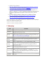
7. Glossary
Term
AffyID
Definition
An identifier for a probe-pair set.
Affymetrix
The largest company which manufactures (single-channel) high-density
oligonucleotide microarray chips.
CDF file
Chip Description File. Describes which probes go in which probe sets
and the location of probe-pair sets (genes, gene fragments, ESTs). See
http://www.bioconductor.org/metaData.html
CEL file
Cell intensity file, including probe level PM and MM values.
Cell line
Cells grown in tissue culture, representing generations of a primary
culture.
DAT file
Image file, approximately 10^7 pixels, approximately 50 MB.
Genotype
The type of RNA in a biological sample as described by the DNA
sequence, e.g. using Single Nucleotide Polymorphisms (SNPs) or
microsatellite markers.
MAS 5.0
The main microarray analysis software from the Affymetrix company:
MicroArraySuite-MAS, now version 5.
The same as PM but with a single homomericbase change for the
middle (13th) base (transversionpurine<-> pyrimidine, G <->C, A <Mismatch(MM)
>T). The purpose of the MM probe design is to measure non-specific
binding and background.
Perfect
match(PM)
A 25-mer complementary to a reference sequence of interest (e.g., part
of a gene).
Phenotype
The type of RNA in a biological sample as described by physical
characteristics of the biological sample, e.g. time or estrogen
presence/absence or observed susceptibility to disease.
Probe
An oligonucleotideof 25 base-pairs, i.e., a 25-mer.
Probe-pair
A (PM,MM) pair.
Probe-pair set
A collection of probe-pairs (16 to 20) related to a common gene or
fraction of a gene.
RMA
Robust Multichip Averaging (Irizarry et al. [6]).
Target
A type of RNA under a particular condition (e.g. Estrogen present)
which is hybridized to a microarray chip.