Download DPTOOLS - fMRITools

Pr. Denis Ducreux's
DPTOOLS
Version 5
By Emeline LAMAIN, MER
LIMEC, INSERM UMR 788
Service de Neuroradiologie Diagnostique et Thérapeutique, CHU Bicêtre, France
DPTools version 5
Requirements
The DPTools software was coded in Delphi, uses the Dr Martin Sanders Optivec © Math
Library, and runs on Windows ® systems (Windows Seven, Vista, XP 32 and 64 bits). It
was optimized to use multiprocessing workstations (SMP).
At least 1024 MB of RAM are needed to process Diffusion / Perfusion files, and 2 GB for
Fiber Tracking with an OpenGL compatible video card.
Cautions
This software is provided ‘as is’, and is involved in many medical scientific research
projects, but is not FDA approved. You can not use DPTools for clinical purposes.
2
DPTools version 5
Chapter I : General Informations
p5
A –Installation, First Run
p5
B –Loading Images
p8
C – Displaying Images
p 15
D- Regions of Interest :
p 21
E- Images Overlay
p 26
F- Filming, Images Saving
p 27
G- Scripting
p 28
Chapter II : MR Diffusion Processing
p 29
A- Trace :
p 29
B- Tensor :
p 31
Chapter III : Dynamic series processing
p 42
A- Perfusion
p 42
B- Permeability :
p 51
C- Flow
p 55
D- Activation
p 56
3
DPTools version 5
Chapter IV : Statistics
p 61
A- Preparing series for statistic processing
p 61
B- Coregistration
p 61
C- Maps creations
p 62
D- Importation / Thresholding
p 63
E- MPR / 3D Surfacic reconstructions
p 64
Chapter V : DPTools preferences
p 71
Chapter VI :DPTools DTI Gradients Scheme
p 73
Chapter VII :References
p 75
4
DPTools version 5
Chapter I: General Usage Principles
I. A – Installation, First run
To install the software, use DPTools-Full-Install.exe. The program will be installed in
the folder “D:\DPTools” by default, but you can change drive (C:, D:, etc…). It is
mandatory to install DPTools in the root directory (eg c:\DPTools) A shortcut will be
generated in the menu Windows. To uninstall the whole program use <<uninstall>>.
NB: The data (diffusion, perfusion, etc…) must be located on the same drive as
DPTools (e.g. C:, D:, etc…) but you are free to put them in the folder of your choice.
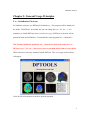
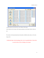
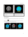
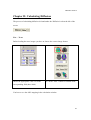
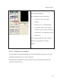
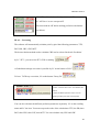
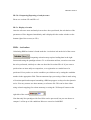
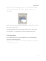
When software is correctly installed, launch DPTools. The cover page of the software
will appear:
Click on one of the pictures in order to start the program.
5
DPTools version 5
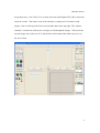
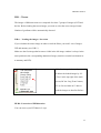
In a general way, ‘Left Click’ (LC) executes an action, and ‘Right Click” (RC) selects the
action to execute. The main screen of the software is composed of 2 windows with
images. One is in the top left of the screen and the other in the top right. The window
contains 2 vertical bars with arrows serving to scroll through the images. The bar on the
top (the larger one) is the axis of Z, and the bar on the bottom (the small one) serves as
the axis of time.
6
DPTools version 5
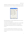
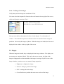
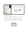
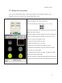
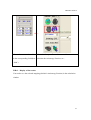
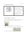
When DPTools is installed on the root directory of your hard disk, you have to configure
it before the first time use. Click on the ‘Configure’ button on the right part of the screen.
Many default settings may be set using this configuration utility; just leave your mouse
cursor on a label, and a hint will pop up.
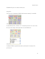
It is mandatory to set the right Diffusion Tensor gradient scheme, for exemple ‘GEHDx’
as shown here for the General Electric HDx MRI systems. Other manufacturers
(Siemens, Philips) are provided, and you can create your own gradients scheme (see
section VI).
If you plan to use DICOM Query/Retrieve and Push functions, you have to set the
network nodes (IP Adress, Port, AE Title) as well as the AET and Port of the DPTools
workstation.
7
DPTools version 5
I.B – Loading Images
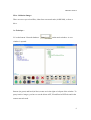
Loading of the images in DPTools is compatible with the following image formats:
DICOM, Siemens Mosaic DICOM Files, Genesis, IMA (Siemens), PAR (Philips),
Analyze, GIS (Raw format), Pixies and in writing with DICOM color, DICOM grayscale,
Analyze and GIS. Before loading the images, you must know their format. DPTools will
try to autodetect the correct image format, but may fail.
In this case, Select this format in the menu to the top right of the screen by
LC on the arrow on the File Type Selection box.
Next to the File Type Selection box are 2 buttons: ‘Img Trans’ and
‘Contrast’. RC on this button to show a pop up menu. LC on an item to
select it.
‘Img Trans’: Basic images post-processing
• Little/BigEndian: Selects the type endian of the file. On a PC, the
files are “Little Endian’, on Sun, they are ‘Big Endian’.
• Intensity scaling: to adjust luminosity
• Invert Order: Classifies the images to load in increasing or
decreasing order either in the 'Z' axis or in time ('T').
• Cubic Interpolation: Do a tri-linear interpolation on the loaded data
• Flip Left-Right: Flip images
• Linear Order: When images are stored in time-dependant series.
• XY Half size: only half size of the picture is used
• Reslice
‘Contrast’: Image contrast type (MRI T2, T1, CT and Anatomy).
8
DPTools version 5
I.B.a – Diffusion Images
There are two ways to load files, either from a network node (in DICOM), or from a
drive.
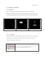
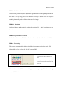
1st Technique :
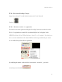
LC on the button ‘Network database’
on the main windows. A new
window is opened :
Remote (in green) and local (in blue) exams are in the right or left part of the window. To
query/retrieve images, you have to set the dicom AET, IP and Port in DPTools and in the
remote network node.
9
DPTools version 5
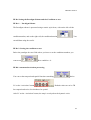
Type in the 'Patient Name' or 'Study Date' field the requested informations, select a
network node by LC on it, then click the blue arrow. Results from the search will be
displayed. To import a sequence, click on the crosses tree until text with '... \DPTools\...'
is displayed. Select the sequence by LC on this text, then LC on the green arrow.
When retrieve process is done, images are displayed in the local DPTools database (left
side of the window)
Use the same process of LC on the crosses tree until the text with '...\DPTools\...' is
displayed, LC on this text to select it, then LC on the ‘Load diffusion serie’ button (red
square on the picture).
2nd Technique :
On DPTools home, LC on the button ‘Load Diff’ to load the diffusion images.
Select the group of necessary images (for example, all of the pictures labeled ‘storkedwi_*.dcm), then LC on ‘Open’.
10
DPTools version 5
A gauge indicates the progression of the loading of the images.
Once loaded, the first image of the first group appears in the image window to the top
left.
The software will automatically detect the number of diffusion directions as well as the
image order.
For Dicom format, only dicom images have to be in a specified folder. If other files
are present, there will be a loading error message !
11
DPTools version 5
Control if the b value is correct on the left of the screen :
12
DPTools version 5
I.B.b – Dynamic Images
You must know if these pictures were obtained in T1 or T2. Set the image contrast by RC
on ‘Contrast’ button, then LC on T1, T2, etc…
After having defined these parameters, load the anatomical images:
LC on the network database, selects the anatomical sequence and LC on the button 'Load
dynamic serie’
2nd method :
LC on the button ‘Load Dyn’ in the top right of the screen, and select all the files (LC on
the first file then ‘CTRL A’). Then LC on ‘Open’.
A gauge indicates the progression of the loading of the pictures. Once loaded, the first
image of the first volume appears in the image window in the top right corner.
13
DPTools version 5
I.B.c : Loading the images of Permeability/ Anatomy / Reference Images
The loading of these types of images is based on the same principles as the loading of the
images of perfusion (permeability) or diffusion. For example if you want to superimpose
ADC maps on T1 volume, first load T1 volume as dynamic, then load diffusion, process
the diffusion, and either mixed/MPR-3D then results (see sections III-D and IV-E).
14
DPTools version 5
I. B.d – Loading of flow images:
Verify that your flow images are encoded on 12 bits.
You must select the adequate file format in the scroll menu in the top right of the screen,
while specifying the extension ‘Flow’.
‘GE flow’ means Genesis format
‘DICOM flow’ means DICOM format.
Next you must indicate the number of slices to load, and put ‘1’ as the number of
volumes. The remainder of process is the same as the one described for the images of
perfusion. Select only the images of phases. When the images are loaded, the first one is
displayed in the window in the top right of the screen.
I.C. Display
When the images are loaded, they are displayed in the image windows. The display can
seem strange or completely black. This can be due to two reasons: the light of the
images is inappropriate or the threshold of the images is too high. By RC on one of the
image windows, you have access to a menu of image properties:
•
Brightness: to brighten the image.
•
Zoom: to enlarge a portion of the image.
•
FOV: to enlarge the entire image.
•
Cursor Position: to position the cursor on a section of the image.
15
DPTools version 5
I.C.a. Windowing / Thresholding
I.C.a.1. Brightness :
By LC on Brightness after having RC on the image window you can change the
brightness of the image. Keep the left mouse button down and move your mouse. You’ll
see the image get brighter (move toward the top left or darker –toward the bottom right).
I.C.a.2. – Threshold:
The threshold of images consists of putting to 0 every pixel that has a value outside of the
threshold values. The threshold of images is done by moving the cursors of the tab
“Threshold’ on the top left of the screen.
The ‘Diffusion Threshold’ refers to the image window in the
top left. The “Low” and “High Perfusion Threshold” to the
image window in the top right of the screen.
16
DPTools version 5
When RC on the threshold bar, you get access to a pulldown menu that allows you to set a threshold for the
diffusion/perfusion images or the charts when these are
being calculated.
I.C.b. Changing the image quality:
By clicking the button ‘Smooth’ in the bottom right of the screen, all images are
smoothed with a spline filter, improving the quality and reducing the pixelization effect
(especially visible in images with a weak matrix or that are zoomed in strongly.
You can adjust the additional Gaussian smoothing using the scrollbars near the ‘Smooth’
button.
17
DPTools version 5
I.C.c. – Zoom in/out on images:
You can either enlarge the whole image (FOV) or use a magnifying glass to enlarge a
part of the image temporarily (Zoom).
I.C.c.1. FOV – Field of View:
RC on the image window, then LC on FOV allows you to enlarge the image. To do this,
keep the left mouse button down while you move your mouse. You’ll see the image get
bigger (cursor to the top left) or get smaller (cursor to the bottom right).
18
DPTools version 5
The enlargement values of the FOV are indicated under the image.
I.C.c.2. Zoom:
RC the image window, then LC ‘Zoom’ allows you to enlarge part of the image by using
a magnifying glass. To do this, keep the left mouse button down on the image while
moving your mouse. You’ll see a part of the image enlarged surrounded by a red square.
19
DPTools version 5
I.C.d. Cursor:
RC on the image window and then LC on the ‘cursor’ to get the coordinates of the cursor
proportionate to the size of the image. You can make the cursor visible as a red cross by
clicking: ….
20
DPTools version 5
You can re-center the image in X and Y and you can pivot it (α) by moving the horizontal
cursors. To make your selection, LC “align’. To de-activate the red cross, LC on it.
I.C.e. Colors:
You can choose to view the image in B&W or in color. LC
the button with the color gradient to see in color, the one avec
the B&W gradient to see B&W.
Preset display color scales are also provided (from red to
blue), next to the Color / B&W buttons.
You have some parameters indicated on the left of the screen:
I.D - Regions of Interest:
The Regions of Interest (ROI) can either be drawn automatically following a squared
circle of variable sizes or manually, by circling the Region of Interest. There are a
maximum of 8 ROIs that can each contain a large number of pixels.
21
DPTools version 5
The different ROIs are represented by a unique color code (red, green, yellow, etc.)
which allows you to find them on the image. The values of each ROI are calculated
depending on the calculation (mean, deviation, minimum, maximum).
To place a ROI you have to first select the ‘Cursor’ function in the image window
(1.C.d.).The ROI functions are on the bottom left of the screen.
I.D.a. Automatically round ROI
To place a ROI, LC the icon:
Then choose the surface of your ROI by moving the cursor on
the horizontal bar. The surface of the ROI will be visible above
(here 77 mm2).
If you want to move an ROI, LC on
in the image window
while moving your cursor.
22
DPTools version 5
Once active, position a ROI by LC the
The corresponding ROI is also visible in
image window.
the calculation window (white circle).
I.D.b. Manual ROI
You can draw a ROI manually. LC the image window and choose ‘Cursor’. Do not select
ROI (don’t LC
). Keep the left mouse button down, push ‘shift left’ at the same
time and circle the selected area by moving your cursor.
23
DPTools version 5
The selected area will then appear following the number of the color of ROI in the image
window and in white stripes in the calculation window.
I.D.c - Deleting parts of all of ROI:
You can delete a ROI by LC on the color code of the ROI in the
bottom left of the screen.
To delete all ROI, LC on:
I.D.d. exporting/importing ROI
You can save the drawn ROI and load them later. Click on ‘ROI load’ to load or on ‘ROI
save’ to save the ROI either in Analyze or Raw format in the import/export zone at the
right of the screen.
I.D.e. Display and export of results:
Once the ROI is positioned the obtained values are displayed in the result window on the
bottom right of the screen. Different values are displayed according to different
calculations.
24
DPTools version 5
•
You can enlarge this result window by double-clicking it;
another result window will then appear in the middle of the
screen. It can be behind the main screen. You only need to
move it to find it.
• You can save the results as a text file or as an Excel file by
typing F1 when your cursor moves onto the result window.
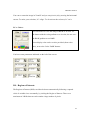
I.D.f. How to create a mask
There are to ways to create a mask. The first method uses a defined circle of the area you
want to keep or delete by using the manual ROI function (1.D.b.), then push F3, F4, F6 or
F7 once while moving the cursor of the mouse on the pertinent image window.
•
F3 – keeps the selection that is circled and erases the rest of the visible
slice.
•
F4: erases the selection and keeps the rest on the slice.
•
F6: keeps what has been circled and erases the rest on the visible slice in
all the volumes
•
F7 Keeps what has not been circled and erases the rest on all the slices of
all the volumes.
25
DPTools version 5
The second method uses a extract brain mask by LC on the ‘Mask’ button
near the Image type combo-box. This function is only working with
T2-w MRI sequences.
I.E. Images Overlay
This function allows you to superimpose the image of the image window on the top left
of the screen with the image of the calculation window in the bottom right. You can stack
with or without smoothing activated (button ‘Smooth’, 1.C.b.), for example Diffusion and
Perfusion results.
LC on ‘mixed’ on the right of the screen.
The transparency of the images can be adjusted with the
horizontal cursor.
26
DPTools version 5
I.F. Filming and saving images
You can save and print the images of the image window, the calculations and the curves
obtained in the curves window in the bottom right of the screen.
LC on ‘Film’ in the bottom right of the screen. The Film Composer
window will appear in the center of the screen.
You can select the size of the images (1, 2, 4, 6, 12, 16).
The text zones hold the notes available as well as the name of the
patient and date of the study.
To send an image to the Film Composer you have to position your
cursor on an image window (calculation or curves), hit F1 and
move your cursor (for all images, hit F2).
- To print your Film Composer, LC ‘Print’
- To select the printer to use, LC ‘config’
- To save your Film Composer as a JPEG, LC ‘Save’
- To adjust the export quality of your Film composer, move the
cursor next to the ‘Save’ button.
- To delete the Film composer, LC ‘Clear’. Changing the image
format will not erase the text fields.
- The film composer can easily be hidden behind the main screen.
You just have to move the various open windows around to find it.
27
DPTools version 5
I.F. Scripting
You can automate the post-processing: LC on the button ‘SCRIPT’ to register
Scripts are text files designed using file type (Dicom, GIS, Analyze, ...), contrast (T2, T1,
CT, Anat), Low Threshold, High Threshold, AIF type (LOCAL, GLOBAL) and position
(x y z), and functions (FILE, PFILE, MSAVE, TIMESHIFT, DIFF, PERFL, PERF,
TENS, CLEAR, ROI x y z, aso...). It must end by 'EOF'.
Here is an example :
GIS
T2
450
8192
LOCAL
FILE
\batch\temoin10
TIMESHIFT
AIF
71
66
5
PERF
ROI
71
68
9
CLEAR
PFILE
\batch\PWITemplate\T1Coreg
AIF
73
58
7
PERFL
MSAVE
CBV
GIS
\batch\PWITemplate\T1Coreg-CBV
CLEAR
EOF
28
DPTools version 5
Chapter II: Calculating Diffusion
The process of calculating diffusion is found under the ‘Diffusion’ tab on the left of the
screen.
II.A. – Trace
Before loading the trace images you have to choose the correct image format.
choose the appropriate value of b in the
LC on the ‘ADC’ button to calculate ADC.
corresponding field (here 1000)
You have to see the ADC mapping in the calculation window.
29
DPTools version 5
If you wish to change the window coloring, RC on the calculation window, then select
‘Brightness’ by LC and then LC the image by moving your cursor (I.C.a.), or use the
preset color-scales buttons (right part of the screen).
Likewise you have access to the other function of ‘Cursor’ for the positioning of ROIs
(I.C.d.), ‘Zoom’, and ‘FOV’ for the enlargements (I.C.c.). when you change FOV of the
calculation window, the FOV of the corresponding image window is automatically
adjusted.
You can also change the diffusion threshold by moving the position of the ‘Diffusion
Threshold’ cursor in the top left of the main screen.
30
DPTools version 5
II.B. – Tensor
The images of diffusion tensor are composed of at least 7 groups of images (6 DTI and
the b0). Before loading the tensor images you need to select the correct image format.
Number of gradients will be automatically detected.
II.B.a. – Loading the images : Inversion
If you calculate the tensor image in order to track the fibers you need 2 sets of images:
DTI and anatomy (see II.B.5.)
Make sure the first image that becomes visible in the left image window is always in the
same position as the corresponding anatomical image (cranial or caudal, but identical as
to anatomy and DTI).
If the first image is inverted you need
to delete the loaded images by LC
‘Clear’ in the top right of the main
screen, RC the ‘Img Trans’ button,
LC on ‘Invert Order in Z’ then reload the images as described before.
III.B.b. Correction of EPI distortion
You can correct your DTI data in 2 ways
31
DPTools version 5
Correction of distortions due to diffusion
gradient ; double-click on then curve graph
in the top right of the screen.
Correction of distortion due to the EPI
sequence: this correction requires a phase
map. Click on ‘Unwarp’ in the left of the
screen under the ‘Diffusion’ tab.
II.B.c. – Processing
Once the diffusion images have been loaded correctly you can make your calculations.
The ‘tensor’ calculates the real values and the real vectors of the acquisition matrix and
calculates the Anisotropy fraction, the Anisotropy ratio, the Volume Ratio, the ADC in
the main axes, the mean ADC etc… The ‘Trace’ button will compute the trace image
from the DTI set after having computed the FA, VR, etc….
32
DPTools version 5
Choose the correct value of b
LC on the ‘Compute Tensor Parameters’ button to
in the corresponding field (here calculate the Anisotropy Fraction, etc…
‘1000’)
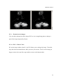
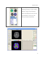
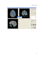
II.B.d. – Display of the results
You need to see the selected mapping (default is Anisotropy Fraction) in the calculation
window.
33
DPTools version 5
You can display another map (for example
(Anisotropy Fraction). LC on the scroll bar
under the ‘Compute Tensor Parameters’
button in the diffusion tab on the left of the
screen and then LC the item you wish.
The map will update automatically.
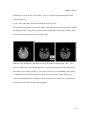
34
DPTools version 5
Take care of the FA results as they reflect the correct DTI gradients scheme. Corpus
callosum have to be in red like in this image. If not, your DTI gradient scheme may be
wrong, and you have to check the ‘Configure’ button to see if declared DTI gradients
match your MRI system.
If you want to change the color scale of the window, RC on the calculation window, then
choose ‘Brightness’ by RC, then LC on the image while moving your cursor (I.C.a.)
In the same way you can access the other ‘Cursor’ functions for the positioning of ROIs
(I.C.d.), ‘Zoom’, and ‘FOV’ for the enlargements (see I.C.c.). when you change FOV of
the calculation window, the FOV of the corresponding image window is automatically
adjusted.
You can also change the diffusion threshold by moving the position of the ‘Diffusion
Threshold’ cursor in the top left of the main screen (see I.C.a.).
II.B.e. – Exporting/Importing maps
Once the calculations have been made, you can save the results.
•
Saving in the 32 bit ‘RAW’ format will allow reloading the results for new
calculations
•
Saving in the DICOM color or B&W format (depending on the display of
the images in color or B&W, see I.C.e.) to integrate into a PACS for
example.
35
DPTools version 5
•
Choose the type of map for export by LC the scrolling
menu in the bottom of the import /Export zone (here
‘ADC’)
•
LC ‘Map save’ to export the maps
•
Choose the format DICOM or GIS and click ‘Save’
•
LC ‘Map Load’ to load the maps. Be careful, only the
maps that were saved as RAW Gis can be re-read.
II.B.f. – FiberTracking
Once you have loaded and calculated the DTI images, you have to load the anatomical
images in the window on the top right of the screen.
II.B.f.1. – Loading anatomy
LC on the button ‘Network database’ to load the diffusion images. A new window is
opening :
36
DPTools version 5
Import the Diffusion images from server in the database. Select the right sequence and
LC on button ‘load diffusion serie’.
or
To load the anatomical images, choose “MRI Anatomy’ in the pop up menu of the
‘Contrast’ button (RC then LC). Then check in the parameter zone that the number of
slices corresponds to the indicated number and that the number of volumes is set to ‘1’.
(see I.B.b.). then LC ‘Load Dyn’ and select your anatomical images.
The DTI images and the anatomical images must have the same cranio-caudal orientation
(identical 1st slice position). If the DTI images don’t correspond to the anatomical ones,
invert them using the previously described method and re-load your anatomical images.
NB: Do not LC ‘Clear’ because this will erase all your calculated images.
37
DPTools version 5
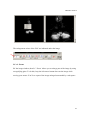
II.B.f.2. Cortex extraction
The extraction algorithm of the brain used is BET (FSL, see ‘References’).
To extract the brain based on the anatomical images, LC on
‘Extraction’ in the MPR/3D tab on the left of the screen.
You may also extract brain using FA values by RC on ‘Extraction’
then LC on ‘Tensor’. You’ll have to set the FA thresholding values
to do so.
You can change the extraction parameters by changing the values of
the underlying fields (here 0.30 and 0.8)
•
The first field (here 0.30) corresponds to the degree of
smoothing of the extraction
•
The second field (here 0.8) corresponds to the value of the
median filter used for binarization.
The files created correspond to the extracted brain (brain.hdr’ and ‘brain.img’) and to the
binarised mask of the latter (‘mask.hdr’ and ‘mask.img’) and are saved in the anatomy
folder ‘…\Brain\’.
The brain extract appears in the calculation window; you can scroll through the slices by
moving the horizontal arrow on the right of the right image window. When you regulate
38
DPTools version 5
your brain extraction parameters, make sure that the brain folds in the final image are
visible from the vertex to the temporal lobes.
II.B.f.3. DTI / Anatomy registration
The adjustment algorithm used is the FSL algorithm (see References)
39
DPTools version 5
•
Select the type of co-registration by RC
‘CoRegister’ in the ‘MPR/3D’ tab, then
load the anatomical images.
•
When the images are loaded, LC
‘CoRegister’ on the left of the screen in
the ‘MPR/3D’ tab.
•
The DTI images are adjusted to the
anatomical ones and a transformation
matrix ‘b0.mat’ is created. All files are
saved in the tensor folder ‘…\DTI\’.
II.B.f.4. FiberTracking
To perform fibertracking, MedInria must be previously installed in the
‘\DPTools\MedInria’ folder of your hard disk (see http://wwwsop.inria.fr/asclepios/software/MedINRIA/).
When the DTI and anatomical files are loaded and adjusted, the ROI have been defined
and the cortex has been extracted, you can start tracking the fibers.
40
DPTools version 5
II.B.f.4.a. Carrying it out
To track the fibers, RC on ‘Fiber Tracking’ in the ‘Diffusion tab on the left of the screen.
to select the image orientation (Axial, Sagittal or Coronal) by LC, then LC on ‘Fiber
Tracking’
Once obtained, the results stay available in the folder ‘…\DTI\’.
II.B.f.4.b. – Loading of an earlier calculation
You can re-use DTI’s, anatomies etc. that have already been calculated. Simply load the
DTI files (see I.B.a.2.) then LC ‘FT’ in the ‘Diffusion’ tab on the left of the screen.
41
DPTools version 5
Chapter III: Calculating dynamic images
Calculating dynamic series is found under the ‘Dynamic / Activation’ tab on the left of
the screen.
III.A. – Perfusion
Before loading trace images, you need to select the correct image format.
III.A.a. – choosing the type of image (T1/T2/CT) and loading
The perfusion calculations are based on the evolution of the signal in time. This signal
evolves differently depending on the method you use, MRI T1 or T2, or CT. You have to
choose this method (MRI T1-w or T2-w, or CT ) before loading the perfusion images by
RC on the ‘Contrast’ button on the top left of the screen until the right option appears.
Then you can load your images as described in section I.B.b.
III.A.b. – Spatial Coregistration
The algorithm of space adjustment used is the one by Woods. It allows for reduction of
side-effects due to movement by the patient.
To apply the adjustment, double-click on the Graph. A
registration graph will appear in the underlying
window.
42
DPTools version 5
III.A.c. – Temporal Coregistration
The series of perfusion obtained in MRI are usually intertwined. This means there is a
substantial time difference of about ½ TR between the first slice and the middle slice.
If the TRs are long (>2s), it is strongly recommended to adjust the series for time in order
to correct the time difference at acquisition.
In the ‘Dynamic’ tab, LC ‘T. Shift’. This
will launch the time adjustment algorithm
based on a bilinear interpolation of the
signal.
NB: the time adjustment has to be done first
- before the space adjustment and the other
calculations of perfusion such as the
selection of AIF etc.
43
DPTools version 5
In the ‘Dynamic’ tab, LC ‘Clone’.
You modify the Baseline.
RC on the button “clone” and choice :
•
Av baseline clone: to average
baseline
•
Baseline clone: to spread baseline
•
Extrapolate endline: if the contrast
injection is not over before the end of
the sequence, you extrapolate the end
of the curve.
You can select the kind of filter: Gaussian
Smooth, Law Pass Filter or LP filter
Display.
III.A.d. – Elimination of recirculation
The elimination is obtained by adjusting the arterial and capillary functions by a model
combining de functions ‘power’ and ‘exponential’.
The adjustment of the data has to be selected before any calculation of perfusion and
before the selection of AIF.
44
DPTools version 5
LC on ‘GFit’ under the ‘Dynamic’ tab on the left of the screen
This adjustment of data sometimes generates wrong results if the adjustment does not fit
well with the experimental data, especially in the case of perfusion in MRI T2-w. Always
verify the quality of the adjustment when you choose your AIF (see next section).
III.A.e. Definition of AIF
AIF = Arterial Input function.
This parameter is very important for the quantitative study of perfusion in T1, CT and T2.
In the software there are 2 types of AIF determination:
•
Global AIF: reflects the mean arterial vascularization calculated based on all the
pixels of all the images
•
Local AIF: AIF is calculated from a group of 9 voxels called ‘arterial’.
By the way, there are 2 ways to determine AIF
45
DPTools version 5
•
Automatically by LC on
•
Semi-automatically : user selects on image of voxels assumed ‘arterial’.
It is strongly recommended to use the semi-automatic method with the local
determination of AIF.
III.A.e.1. Global/local determination
To use a global AIF, RC on ‘AIF’ under the perfusion tab on the left of the
screen, then LC ‘global AIF’.
To use a local AIF, RC on ‘AIF’ under the perfusion tab on the left of the screen,
then LC ‘local AIF’.
III.A.e.2. – calculating and displaying AIF
This section describes the semi-automatic method of determining AIF.
If you wish to use the automatic method, skip to point 5 (no reference area).
Choose in the image window on the right the slice representing the polygon of Willis.
Use the little vertical arrow on the right of the image to scroll through the slice on the Taxis in order to visualize the contrast (the vessels turn black)
RC on the image and LC on the AIF item of the scrolling AIF menu.
46
DPTools version 5
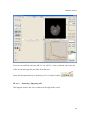
Position your cursor on the vessel and LC on it; a red square representing the arterial
reference appears.
LC on ‘AIF’ under the perfusion tab on the left of the screen.
The arterial pixels appear in red on the image; check their intra-arterial position by letting
the images scroll by using the big vertical arrow on the right of the image window. Then
press F5 while moving your cursor on the image.
Make sure the adjustment of the data is correct If you have activated the ‘GFit’. You
must see a blue curve corresponding to the average of the variations of the signal in the
selected area (red square on artery). You’ll see a red curve corresponding to the average
of variations of all the arterial pixels of all the slices of the study and a yellow curve
which is the adjusted curve of the data. Please make sure the yellow curve joins the base
line and fits well to the red line in the beginning.
47
DPTools version 5
If you are not satisfied with your AIF, LC on ‘AIF CL’ in the ‘perfusion’ tab on the left
of the screen and begin the procedure from the start.
Some AIF interpolation may be needed, just LC on ‘Interp’ button
III.A.e.3. – Exporting / Importing AIF
This happens in the Load / Save window on the right of the screen
48
DPTools version 5
LC “AIF Load’ to load an already calculated AIF
LC ‘AIF Save’ to save an open AIF
You must load an AIF before making perfusion calculations
(see below).
III.A.f. – Processing
The software will automatically calculate pixel by pixel the following parameters: TTP,
BAT, DR, CBV, CBF, MTT.
The deconvolution method used to calculate CBF can be selected in the tab ‘Perfusion’
by LC ‘FFT’; you can select FFT, SVD or nothing.
A Gadolinium leakage correction is possible by LC on the button “Gd LC”
To have T1CDecay correction, LC on the button “Decay Fit”
LC on ‘Compute Perfusion Parameters’ in the tab
‘Dynamic’ on the left of the screen. The calculation will
continue.
To display the different perfusion maps, LC on the
underlying scrolling menu and LC the right item.
You can also calculate the different perfusion parameters separately. LC on the scrolling
menu and LC the item. You must respect the order of the calculations: TTP, the DR, then
BAT, then CBV, then CGF, then MTT. You can calculate only CBV and CBF.
49
DPTools version 5
CBF (Cerebral Blood Flow)
MTT (Mean Transit Time)
III.A.g. – Display of results
Once the calculations have been made, if you want to change the coloring of the window,
RC on the calculation window, then choose ‘Brightness’ by RC, then LC on the image
while moving your cursor (I.C.a.)
In the same way you can access the other ‘Cursor’ functions for the positioning of ROIs
(I.C.d.), ‘Zoom’, and ‘FOV’ for the enlargements (see I.C.c.). When you change FOV of
the calculation window, the FOV of the corresponding image window is automatically
adjusted.
You can also change the diffusion threshold by moving the position of the ‘Diffusion
Threshold’ cursor in the top left of the main screen (see I.C.a.).
CBF – Cerebral blood flow // MTT – Mean Transit Time
50
DPTools version 5
III.A.h. – Export /Import of maps
Once the calculations have been done you can save the results.
The procedure is identical to the one described under II.B.e.
III.A.i. – Images Overlay
It is very useful to see the ischemic shadow zone to be able to stack diffusion images and
perfusion maps.
Once loaded, the perfusion images have to be calculated. You can then load the diffusion
images by using the ‘Mixed’ function in section I.E.4.
III.B. Permeability
Calculation of permeability is based on the bi-compartimental model (refs in section VII)
and may use T1-w or T2-w images.
III.B.a. Selection and loading of images
Before you load your permeability images you need to select the right modality IRM, T2,
T1 or CT by clicking the ‘Contrast’ button on the top left of the screen until the correct
text appears.
Adjust your ‘Perfusion Threshold” so that you see the parenchymatic structures correctly.
Then load your images as described in I.b.b.
51
DPTools version 5
III.B.b. – Definition of the zones of analysis
Calculation of permeability uses adjustment algorithms of Levenberg-Marquard and can
turn out to be a very long process. It is therefore necessary to define a zone of analysis by
outlining it manually and to eliminate the rest of the image.
III.B.b.1. – Outlining
Outlining is based on the principle explained in section I.D.f. – only keep what needs to
be analyzed.
III.B.b.2. Export/Import of areas
Outlined areas behave as ROI and can be loaded or saved as described in section I.D.d.
III.B.c. – Processing
The software automatically calculates the following parameters pixel by pixel: KPS
(Permeability of the surface), K1, K2, K Total and fBV.
LC on permeability under the “Perfusion’ tab
on the left of the screen. Calculation will
follow.
To display the different permeability maps, LC
on the underlying scrolling menu and LC the
chosen item.
You can also treat the different permeability parameters separately; LC on the scrolling
menu and LC the item.
52
DPTools version 5
III.B.d. Display of results
Once the calculations have been made, if you want to change the coloring of the window,
RC on the calculation window, then choose ‘Brightness’ by RC, then LC on the image
while moving your cursor (I.C.a.)
In the same way you can access the other ‘Cursor’ functions for the positioning of ROIs
(I.C.d.), ‘Zoom’, and ‘FOV’ for the enlargements (see I.C.c.). When you change FOV of
53
DPTools version 5
the calculation window, the FOV of the corresponding image window is automatically
adjusted.
You can also change the diffusion threshold by moving the position of the ‘Diffusion
Threshold’ cursor in the top left of the main screen (see I.C.a.).
The permeability map is displayed in the calculation window on the bottom left. An
average curve of maximum reinforcement is then drawn in the curves window. This
curve corresponds to the variation of the signal in time of pixel group 9 having the
maximum concentration of contrast.
If you position a ROI on the analysis zone, an average curve of reinforcement of the
signal is drawn in the curves window (in red) and is adjusted by the bi-compartimental
model (in yellow). Please check the adjustment quality.
III.B.e. – Export/Import of the maps
Once the calculations have been made, you can save the results. The procedure is
identical to the one described in section II.B.e.
III.B.f. Stacking of images
To see the zone of ischemic shadow it is very useful to be able to stack diffusion images
and perfusion maps. Once loaded the perfusion images need to be calculated. Then load
the diffusion images and use the ‘MIXED’ function described in section I.E.
54
DPTools version 5
III.C. – Flow
The calculation of flow is based on the MRI acquisitions in phase contrast (see refs in
Annex).
The calculation method is very similar to the one described in section III.A.
III.C.a. Selection and loading of images
See section I.B. and I.B.d.
III.C.b. – Definition of analysis zones
To estimate the flow parameters, you need to position a ROI on the analysis zone and an
ROI on the reference zone.
III.C.b.1. – Reference zone
The reference zone needs to be selected in a region of moderate noise without systolicdiastolic signal variation.
The zone uses the semi-automatic local AIF principles.
RC on the image window on the right, then LC on ‘AIF’, then LC on the part of the
image that serves as reference zone. You can have your images scroll by with help of the
large vertical arrow to the right of the image window.
III.C.b.2. – Analysis zones
Are the zones corresponding to the ROIs. Please refer to section I.D.
55
DPTools version 5
III.C.b.3. Importing/Exporting of analysis zones
Please see sections I.D. and III.A.e.3.
III.C.c. Display of results
Once the reference areas and analysis areas have been positioned, the calculation of the
parameters of flow happens immediately and is displayed in the results window on the
bottom right of the screen (see I.D.).
III.D. – Activation
Calculating fMRI activation is found under the ‘Activation’ tab on the left of the screen.
. Computing activation map requires loading data in the right
format and setting the paradigm scheme. To avoid motion artifacts, a motion correction
has to be performed, similarly to what was described in section III.A.b. If you want to
perform inter or intra-subjects comparison, a co-registration to a model has to be
performed. Next you have to set the condition you whish to test by setting the condition
number in the appropriate filed. Then an automated pre-processing of data is made using
a Gaussian spatial and temporal smoothing. fMRI map appear overlayed on the dynamic
series. You may want to use other anatomy or reference file. This can be done either
using volumic mapping (for volume anatomy) or using the ‘3D Interpol’ button on the
right side of the screen
.
Note that only bloc paradigm with fixed SOA can be processed, but you can choose to
compare 2 of the up to 999 conditions. Blocs are convolved with HRF.
56
DPTools version 5
III.D.a. Selection and loading of images
Images have to be by LC on the “load activation serie” in the Network
Database.
III.D.b. – Motion correction / co-registration
The motion correction is performed using the ‘Re-Align’ button as described in section
III.A.b. Co-registration to a model file is performed by RC on ‘Co-Register’ in the
‘MPR/3D’ tab, then LC on ‘PWI to Reference’, then LC on ‘Co-register’. Previously you
have to save the model file in GIS format. DPTools will ask you which file you want to
use as a model, then perform the co-registration.
By modifying the number on the left of the screen under “extraction” , you choice
extraction power thereshold.
57
DPTools version 5
III.D.c Setting the Paradigm Scheme and the Conditions to test
III.D.c.1. – Paradigm Scheme
The Paradigm scheme is presented using a matrix style forme, with on the left cell the
condition number, and on the right cell, the condition duration
. You
can add data using the scrolls.
III.D.c.2. Setting the conditions to test
Below the paradigm box are fields where you have to set the conditions numbers you
want to test
. Rest condition = 0.
III.D.d. Automated Activation processing
You can set the temporal and spatial Gaussian smoothing
LC on the ‘Activation’ button
before
. Defaults values are twice TR
for temporal and twice slice thickness for spatial.
After LC on the ‘Activation’ button, the map is overlayed on the dynamic series.
58
DPTools version 5
III.D.e. Saving maps:
The procedure is identical to the one described under II.B.e. You only have to select the
‘P.Stats’ field for activation maps.
For group studies, you can perform additional statistics on the saved fMRI maps (for
example, mean or Z Score). This can be done in the ‘Statistics’ tab, using the statistics
combo
. See chapter IV.
III.D.f. Displaying maps on volumic / reference images
You can display maps on 2D references files (such as FLAIR, T2, etc…). This can be
done after having saved the activation map in GIS format, then LC on the ‘Clear’ button,
then selecting the ‘MRI Anatomy’ type by RC on the ‘Contrast’ button on the right side
of the screen. Next you have to set the correct slices number in the ‘Serie Slices’ section
in the upper left part of the screen, as described previously, and setting the ‘Serie Phases’
to 1.
Then import your files. LC on the ‘3D Interpol’ button, and LC on ‘Load Map’ to import
previously saved activation map. Map will be overlayed on the reference images.
You can also coregister maps on a volumic anatomy file. This file has to be saved in GIS
format, for example after the cortex extraction procedure, you can LC on ‘Save Dyn’,
select GIS, and save the volume file.
59
DPTools version 5
To perform the coregistration, you need as well a model file of the original fMRI data.
This model file has to be in GIS format. After importing the fMRI data, save them using
the same process (‘Save Dyn’ button and ‘GIS’ format’).
Once you have all your 3 files (anatomy, fMRI model and map) in GIS format, then click
on the ‘Statistic’ tab near the ‘Activation’ tab, and LC on ‘Vol. Mapping’. The map will
be coregistered to the volume with identical dimensions and voxel thickness.
This procedure is available for all the maps generated with DPTools (DTI, PWI, aso…).
60
DPTools version 5
Chapter IV: Statistics:
The statistical operations refer to the image series of diffusion, perfusion and the maps. It
is possible to calculate Mean / Min / Max / SD on several series or maps and to calculate
the Z Score, Chi2 , Pearson, Difference between series or maps.
IV.A. Preparation of the series
Before doing the statistical calculations the series need to be coregistered in comparison
with a template. It is possible to create one’s own template by averaging several series,
all coregistered on one single series.
IV.B. Coregistration
Choose the type of coregistration by RC on
‘Coregister’ under the ‘MPR/3D’ tab and
then load the images to be coregistered
(DTI or anatomical).
You need a GIS template to be able to
coregister your series onto that template. It
is possible to create one by saving in GIS
format loaded images in dicom for example.
Select ‘DTI to reference’ or ‘PWI to
reference’ and LC on ‘Coregister’.
61
DPTools version 5
Once your series have been all coregistered, place them in the same folder on the hard
disk and go to the tab ‘Statistics’ and select Mean / Min / Max / SD’, then LC on
‘STATISTICS’.
The files with average, minimum, maximum and standard deviation will be created in the
folder of your coregistered series.
By modifying the number above button “Gaussian Smth”, you choice source scaling
factor (thereshold). LC on the button “Gaussian smth” to apply smooth Gaussian.
IV.C. Map creation:
Every coregistered series will be treated separately and the maps resulting from this
series will be saved in the same folder.
Likewise, you can do statistical calculations based on maps. The generated maps will be
saved in the folder of your data.
62
DPTools version 5
IV.D. Importing and thresholding
To visualize the statistical maps, you
first need to load a visualization support
(generally the coregistered series).
Then you must load the statistical maps
(‘D. Stats’ or ‘P. Stats’) in the ‘Map
Load’ on the right of the screen.
The threshold will be determined as
described in section I.C.a.
IV.E. MPR / 3D Surfacic reconstructions
After having saved anatomy and processed map (using the ‘Vol. mapping’ button), you
can perform multiplanar reconstructions by LC on the ‘MPR / 3D’ button
in the ‘MPR/3D’ tab. Another window will show up.
You can also load anatomic files by LC on the ‘Load Vol.’ button, and load maps by LC
on the ‘Load Map’ button (GIS format).
.
63
DPTools version 5
Data are smoothed using a Gaussian filter. To deactivate the smoothing, please LC on the
‘Smooth’ button
before loading maps .
If your map file has a different slice thickness or a different slices number compared to
your volume file, you will have to set the reference slice from which the map will be
overlayed on anatomy. This slice has to be the top first one.
By RC on the images, you can select between ‘Brightness’, ‘Cursor’, ‘Zoom’, and ‘Map
Window’. These functions are similar to those reported earlier in the text.
64
DPTools version 5
You can also load previous volume and maps by clicking on ‘Load Vol.’ and ‘Load Map’
buttons, and display maps by LC on the ‘Map I/O’ button on the right of the screen.
You have a bar under this button to adapt the rear projection of the map on the
anatomical image.
You adapt the image visualization (anatomical image and map) with horizontal bar above
‘3D surf’ button, on the right of the screen.
If your volume reconstruction looks inverted, LC on the ‘Invert’ checkbox
on
the right of the screen.
To perform a 3D surfacic reconstruction, you need to have extracted the brain of your
volume file (see sections above), then LC on the ‘Brain extraction’ button in the left side
of the window
.
Then LC on ‘MPR/3D’ to open 3D window.
Then LC on ‘Volume Rendering’ to have the 3D reconstruction.
65
DPTools version 5
The MRIcroGL open a new window with the result.
Setting ROIs :
You can set up to 4 simultaneous 3D ROIs. ROI selection is made by LC on the ROI
color
.
To make ROI on the slice: “shift left + LC”. Verify that your mouse is in ‘cursor’ mode,
RC if you need to change. On the right on the screen, the ROI data are
indicated.
Coordinates of ROI are reported in mm and in voxels from the CA location (if CA
previously set).
66
DPTools version 5
By LC on
, crossbar is shown. You can Load or Save ROI in Analyze format by LC
on the appropriate button. You can enable/disable ROI by LC on
You can also clear only the selected ROI by LC on
clear all ROIs if
if
.
is up, and
is down.
Visualizing a ROI volume is made by LC on
after have make ROI on some
different slices in axial.
Possibility to push F6 or F7 once while moving the cursor of the mouse on the pertinent
image window.
•
F3: keeps what has been circled and erases the rest on the visible
•
F4 : keeps what has not been circled and erases the rest on all the slices
•
F6: keeps what has been circled and erases the rest on the visible slice in
the whole volume
•
F7 : keeps what has not been circled and erases the rest on all the slices in
the whole volume
Visualizing ROI in 3D is made by LC on
after have reconstructed the brain. ROI
measurements are visible in the ROI reports windows, and can be saved by typing ‘F1’
key and moving the mouse on it.
If CrossBar is enabled, then you can see the cursor location in the 3D window.
67
DPTools version 5
68
DPTools version 5
Modify the thresholds to make appeared the mask with horizontal bar on the right of the
screen
.
An automatically ROI, RC on the ‘estimate’ button to choice the typ of region
Then LC on the ‘estimate’button. The results are on the images.
You choice volume selection by RC on the ‘Volume’ button
Once the contrast adapted, select volume on the right of the screen:
69
DPTools version 5
.
70
DPTools version 5
V. DPTools Preferences
Preferences can be set in DPTools using the ‘DPToolsRegistration.exe’ software, found
either on the website (http://www.fmritools.org), or in the ‘\DPTools\bin’ folder of your
installation directory.
This software can set default values of b diffusion gradient, perfusion slices, paradigm
scheme, aso…. All fields have hint text as description.
The software generates the dptools.ini file, found in the ‘\DPTools\bin’ directory.
# DPTools Ini file - Do not change lines order !
# RAMDrive Letter - If none, keep it blank !
# Diffusion Threshold
100
# Diffusion b value
1000
# DTI directions
25
# Perfusion Low Threshold
250
71
DPTools version 5
# Perfusion High Threshold
24576
# Perfusion Phases
25
# Perfusion Slices
18
# Perfusion SA Start
0
# Perfusion SA Duration
5
# Image Format
Dicom
# Perfusion Gamma Fitting On/Off
1
# DPTools Running Key
# DPtools Tensor Extension
PhilipsKB
# PC AE Title
NRDPTNVISUDD
4006
#Node 1 IP and Port
MRSC16511
10.163.222.16
104
#Node 2 IP and Port
MXVIEW1
10.163.222.11
104
#Node 3 IP and Port
NR_SERVER_2
192.168.128.25
4006
#Node 4 IP and Port
NRSRVDIAG
10.163.222.220
4006
#Node 5 IP and Port
MNAVDICOMQR
10.163.222.245
104
#Node 6 IP and Port
BCT-NRMACDD
10.163.222.248
4096
#SMP
1
#TempCor
0.40
#AutoCor
0.1
#Paradigm
14
0
6
1
6
0
6
1
6
0
6
1
6
0
6
72
DPTools version 5
VI. DPTools DTI Gradients Scheme
DTI Gradients scheme can be set in DPTools using a text file found in the ‘\DPTools\bin’
folder of your installation directory. All gradient file names have to begin with
‘Gradients’. For exemple here is the ‘GradientsSiemensOld.txt’ file:
Axial
Sagittal
Coronal
12
6
0.0 0.707 0.707
0.0 -0.707 0.707
0.707 0.0 0.707
0.707 0.0 -0.707
0.707 0.707 0.0
0.707 -0.707 0.0
12
1.000000 0.414250 -0.41425
1.000000 0.414250 -0.41425
1.000000 -0.414250 0.41425
1.000000 0.414250 0.41425
0.414250 0.414250 1.0
0.414250 1.000000 0.41425
0.414250 1.000000 -0.41425
0.414250 0.414250 -1.0
0.414250 -0.414250 -1.0
0.414250 -1.000000 -0.41425
0.414250 -1.000000 0.41425
0.414250 -0.414250 1.0
---------------------------------------------------------------Axial
Sagittal
Coronal
This section defines the order of the rotation matrix to be performed to the gradients set.
It depends on your MRI system.
---------------------------------------------------------------12
The total number of available directions
73
DPTools version 5
---------------------------------------------------------------6
0.0 0.707 0.707
0.0 -0.707 0.707
0.707 0.0 0.707
0.707 0.0 -0.707
0.707 0.707 0.0
0.707 -0.707 0.0
12
1.000000 0.414250 -0.41425
1.000000 0.414250 -0.41425
1.000000 -0.414250 0.41425
1.000000 0.414250 0.41425
0.414250 0.414250 1.0
0.414250 1.000000 0.41425
0.414250 1.000000 -0.41425
0.414250 0.414250 -1.0
0.414250 -0.414250 -1.0
0.414250 -1.000000 -0.41425
0.414250 -1.000000 0.41425
0.414250 -0.414250 1.0
The number of directions followed by the x y z gradients values.
74
DPTools version 5
VII. References
Diffusion Algorithms based on:
A. L. Alexander, K. Hasan, G. Kindlmann et al. A Geometric Analysis of Diffusion Tensor
Measurements of the Human Brain. Magnetic Resonance in Medecine 2000;44:283-291
P. J. Basser, C. Pierpaoli. A Simplified Method to Measure the Diffusion Tensor from
Seven MR Images. MRM 1998;39:928-934
A. M. Ulug, P. C. M. van Zijl. Orientation-Independent Diffusion Imaging Without
Tensor Diagonalization: Anisotropy Definition Based on Physical Attributes of the
Diffusion Ellipsoid. JMRI 1999;9:804-813
D. Weinstein, G. Kindlmann, E. Lundberg. Tensorlines: Advection-Diffusion based
Propagation through Diffusion Tensor Fields. Unpublished data.
Perfusion Algorithms based on:
Boxerman JL, Hamberg LM, Rosen BR, Weisskoff RM. MR contrast due to intravascular
magnetic susceptibility perturbations. Magn Res Med 34:555-566
Calamante F, Thomas DL, Pell GS, Wiersma J, Turner R. Measuring Cerebral Blood
Flow using Magnetic Resonance technics. J Cereb Blood Flow Metab 1999;19 :701-735
Hagen T, Bartylla K, Piepgras U. Correlation or regional cerebral blood flow measured
by stable xenon CT and perfusion MRI. J Comp Assist Tomo 1999;23:257-264
Kennan RP, Zhong J, Gore JC. Intravascular susceptibility contrast mechanism in
tissues. Magn Res Med 1994;31:9-21
Rosen BR, Belliveau JW, Buchbinder BR, McKinstry RC, Porkka LM, Kennedy DN,
Neuder MS, Fisel CR, Aronen HJ, Kwong KK, et al. Contrast agent and cerebral
hemodynamics. Magn Res Med 1991;19:285-292
Smith AM, Grandin CB, Duprez T, Mataigne F, Cosnard G. Whole brain quantitative
CBF and CBV measurements using MRI bolus tracking: Comparison of methodologies.
Magn Reson Med 2000;43(4):559-564
Starmer CF, Clarck DO. Computer computations of cardiac output using the gammafunction. J Appl Physiol 1970;28:219-220
75
DPTools version 5
Wirestam R, Andersson L, Ostergaard L, et al. Assessment of Regional Cerebral Blood
Flow by Dynamic Susceptibility Contrast MRI Using Different Deconvolution
Techniques. MRM 2000;43:691-700
Fiber Tracking algorithms by Pierre Fillard and Guido Gerig:
Pierre Fillard, John Gilmore, Weili Lin, Guigo Gerig, "Comprehensive Analysis of
Diffusion Tensor MRI on your personnal Computer",
Abstract submitted and accepted to the "18th Annual Radiology Research Symposium".
Pierre Fillard, John Gilmore, Weili Lin, Guigo Gerig, "Quantitative Analysis of White
Matter Fiber Properties along Geodesic Paths",
accepted to MICCAI 2003 conference (avril 2003).
Pierre Fillard and Guido Gerig, "Analysis Tool For Diffusion Tensor MRI",
accepted to MICCAI 2003 conference (avril 2003).
Dongrong Xu, Susumu Mori, Meiyappan Solaiyappan, Peter C. M. van Zijl and Christos
Davatzikos. A Framework for Callosal Fiber Distribution Analysis.
T1 Permeability algorithms based on:
Heidi C. Roberts, Timothy P. L. Roberts, Robert C. Brasch, and William P. Dillon.
Quantitative Measurement of Microvascular Permeabilityin Human Brain Tumors
Achieved Using DynamicContrast-enhanced MR Imaging: Correlation with Histologic
Grade. AJNR Am J Neuroradiol 21:891–899, May 2000
Patlak CS, Goldstein DA, Hoffman JF. The flow of solute and solvent across a twomembrane system. J Theor Biol 1963;5:426–442
Tofts PS. Modeling tracer kinetics in dynamic Gd-DTPA MR imaging. J Magn Reson
Imaging 1997;7:91–101
Tofts PS, Kermode AG. Measurement of the blood-brain barrier permeability and
leakage space using dynamic MR imaging, 1: fundamental concepts. Magn Reson Med
991;17:357–367
76
DPTools version 5
T2 permeability algorithm patent WO/2008/132386
http://www.wipo.int/pctdb/en/wo.jsp?WO=2008132386
CSF Flow Analysis routines based on:
Cerebrospinal Fluid Dynamics and Relation with Blood Flow. A Magnetic Resonance
Study with Semiautomated Cerebrospinal Fluid Segmentation. Balédent O., HenryFeugeas M.C., Idy-Peretti I. Investigative Radiology 36;7:368-377
Movements correction algorithm and Image Registration by: Automated Image
Registration (AIR), R. Woods, UCLA, USA (provided "as is").
Woods RP, Grafton ST, Holmes CJ, Cherry SR, Mazziotta JC. Automated image
registration: I. General methods and intrasubject, intramodality validation. Journal of
Computer Assisted Tomography 1998;22:141-154
Woods RP, Grafton ST, Watson JDG, Sicotte NL, Mazziotta JC. Automated image
registration: II. Intersubject validation of linear and nonlinear models. Journal of
Computer Assisted Tomography 1998;22:155-165
Brain Cortex Extraction by: BET (Automated Brain Extraction) - Part of FSL by
Stephen M. Smith, Head of Image Analysis, FMRIB Oxford University Centre for
Functional MRI of the Brain John Radcliffe Hospital, Headington, Oxford OX3 9DU, UK
+44 (0) 1865 222726 (fax 222717)
Smith, S. (2000a). Robust automated brain extraction. NeuroImage. submitted.
Smith, S. (2000b). Robust automated brain extraction. In Sixth Int. Conf. on Functional
Mapping of the Human Brain, page 625.
DICOM routines by D. Ducreux and Chris Rorden, University of Nottingham, UK.
Rorden C., Brett M. Stereotaxic display of brain lesions. Behavioural Neurology
2001;12:191-200
All other routines and algorithms developped by Denis Ducreux.
77