Download PDF

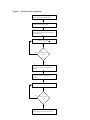
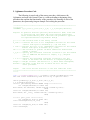
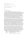
Estimating the Area under a Receiver Operating Characteristic (ROC) Curve
For Repeated Measures Design
Honghu Liu1 and Tongtong Wu2
ABSTRACT
The receiver operating characteristic (ROC) curve is widely used for diagnosing
as well as for judging the discrimination ability of different statistical models. Although
theories about ROC curves have been established and computation methods and
computer software are available for cross-sectional design, limited research for
estimating ROC curves and their summary statistics has been done for repeated measure
designs, which are useful in many applications, such as biological, medical and health
services research. Furthermore, there is no published statistical software available that
can generate ROC curves and calculate summary statistics of the area under a ROC curve
for data from a repeated measures design. Using generalized linear mixed model
(GLMM), we estimate the predicted probabilities of the positivity of a disease or
condition, and the estimated probability is then used as a bio-marker for constructing the
ROC curve and computing the area under the curve. The area under a ROC curve is
calculated using the Wilcoxon non-parametric approach by comparing the predicted
probability of all discordant pairs of observations. The ROC curve is constructed by
plotting a series of pairs of true positive rate (sensitivity) and false positive rate (1specificity) calculated from varying cuts of positivity escalated by increments of 0.005 in
predicted probability. The computation software is written in SAS/IML/MACRO v8 and
can be executed in any computer that has a working SAS v8 system with
SAS/IML/MACRO.
Key words: Receiver Operation Characteristic (ROC) curve; Generalized linear mixed
model (GLMM); Area under ROC Curve.
1. Introduction
Receiver operating characteristic (ROC) curves have been used as measures for
the accuracy of diagnostic tests in medicine and other fields when the test results are
continuous measures. ROC curves display the relationship between sensitivity (truepositive rate) and 1-specificity (false-positive rate) across all possible threshold values
that define the positivity of a disease or condition. They show the full picture of trade-off
between true positive rate and false positive rate at different levels of positivity.
Summary measures of ROC curves, such as the area under the curve (AUC), the
projected length of the ROC curve (PLC) and the area swept out of the ROC curve
(ASC), can summarize the inherent capacity of a test or bio-marker for discriminating a
diseased from a non-diseased subject across all possible levels of positivity into a single
statistic.[1,2]
There is much literature on statistical methods for estimating ROC curves,
calculating the area under a ROC curve and even comparing ROC curves (both
independent and correlated) for cross sectional data.[3,4,5,6] Although not able to
1
From the Department of Medicine (corresponding author), School of Medicine, UCLA. 911 Broxton
Plaza, Suite #202, LA, CA 90095-1736. E_mail: [email protected]. 2 From the department of Biostatistics,
School of Public Health, UCLA. Email: [email protected]
automatically test and compare ROC curves, most of the major statistical software
packages, such as SAS[7], STATA[8] and SPSS,[9] have procedures that can directly
generate a single ROC curve and calculate the summary statistic of AUC under a crosssectional design.
Repeated measures design is widely used in biological, medical and health
services research, but statistical methods for estimating ROC curves and their summary
statistics have been lacking for such designs, especially regression model based
approaches, which provide the opportunity to evaluate the impact of co-variates on the
potency and accuracy of a test or bio-marker. In medical and health services research, for
example, researchers often need to observe the change of patient’s outcomes over time as
a function of treatment, time and other covariates. These outcome measures are often in
continuous format but can be dichotomized by choosing some clinically-meaningful
critical value c and defining the test or bio-marker to be positive if the outcome measure
is greater than c. For instance, we may need to analyze patient cholesterol level over time
as a function of treatment, diet and other patient characteristics; we may need to observe
patient health status measured by SF-36 [10] or SF-12 [11] over time as a function of
process of care and structure of medical organizations; and we may need to study HIV
patients’ virologic outcome as a function of adherence to antiretroviral medication
treatment and other covariates. The inherent longitudinal discriminating power of
treatments and other covariates on outcomes that are measured over time can be analyzed
and evaluated by appropriately calculated ROC curves that take into account the
dependence of observations within a subject. Statistical computation methods and
computer software for such analyses are few and in need. In this paper, using generalized
linear mixed model (GLMM) and a Wilcoxon non-parametric approach, [12] we propose
a model-based method for calculating ROC curves and the area under a ROC curve for
repeated measures design. A statistical software program, written in SAS/ Macro/IML is
specifically designed and created to implement the proposed algorithm and carry out the
computations. With this software, one will be able to fit ROC curves and calculate the
area under a ROC curve for data from repeated measure designs, which currently no
software on the market can handle.
2. ROC curve for cross-sectional data
A ROC curve is a plot of sensitivity versus 1-specificity, where the sensitivity is
defined as the probability that a test result is positive given the subject is truly diseased
and the specificity is defined as the probability that the test result is negative given the
subject is truly non-diseased. Let y ∈ ( −∞, ∞ ) denote the result of a test or bio-marker
with a continuous outcome, D be an indicator of diseased/positive ( D = 1 ) or nondiseased/negative ( D = 0 ) status of a subject, c be a threshold that any test result y ≥ c is
considered to be diseased/positive, and t ∈ ( 0,1) be the false positive rate (1-specificity).
Let FD ( c) = Pr( y ≤ c | D = 1) and FD ( c) = Pr( y ≤ c | D = 0) be the cumulative
distribution function of y for diseased and non-diseased subjects. Then 1- FD (c ) and
FD (c ) will be the sensitivity and specificity, respectively. Let S D (.) = 1 − FD (.) and
S D (.) = 1 − FD (.) be the survival function of y for the two groups, we can write ROC
curves in a succinct form: roc (t ) = S D {S D−1 ( t )} , where t varies from 0 to 1 as the
2
corresponding threshold c varies from ∞ to − ∞ . [13] It has been shown that the area
under a ROC curve equals the unconditional probability of correct ordering, [14] that is
∫ ROC (t)dt = P( y D > y D ) .
Regression models can evaluate the impact of covariates on the accuracy of a
diagnosis test or a bio-marker. When a test or bio-marker is continuous with normal
error, it can be modeled through the standard linear regression model:
y = µ + ε = Xβ + ε
where µ = E( y) is the mean of y and β are the regression coefficients is X . Very
often, these continuous outcomes can be dichotomized by choosing some meaningful
critical value c and defining the test result or bio-marker as positive if it is greater than
the critical value of c. After this conversion, the problem is translated to model the
impact of covariates on binary outcome measures, such as diseased(positive) versus
non-diseased(negative). To model binary outcome measures, one can model functions
of µ rather than µ itself; that is to use generalized linear model (GLM) framework. The
basic form of GLM can be written as η = g ( µ) = Xβ , where η is a link function that
links E ( y) with the linear predictor Xβ . To evaluate the impact of covariates on ROC
curves, one can either model the impact of covariates on a diagnosis test or a biomarker, directly on ROC curve or even on the summary statistics of ROC curve, such
as the area under a ROC curve.
3. Estimating ROC Curve under Repeated Measures Design
Under repeated measures design, each patient will have multiple data points over
time or under different conditions. The observations within a given patient will no
longer be independent and the intra-patient correlation and variation are introduced in
the analyses. Due to intra-patient variation, the impact of covariates on the accuracy of
a diagnostic test or a bio-marker will consist of both fixed global effect (e.g., patient’s
gender) as well as individual patient random effect (e.g., change over time). For both
continuous and non-continuous repeated measure outcome variables, the random
effects from individual subjects can be incorporated in a model through the extension of
GLM to generalized linear mixed model (GLMM),[15] in which the linear predictor
consists of two parts of fixed and random effects.
Let µi = E ( yi | γ i ) be the conditional mean of an outcome variable yi , and let
ηi = g ( µi ) be the link function that connects µi with a linear predictor. Then GLMM
can be written as:
ηi = X i β + Z i γ i
for i=1,…,n.
and the conditional variance is:
Var ( y i | γ i ) = R ,
where yi is a ni x1 vector of test results for the ith patient, ni is the number of outcome
measures for the ith patient, X is n x p containing known covariates that are associated
with the fixed effects. β , the fixed effect parameter vector is px1, and Z i is n i x k
representing known covariates that are associated with the random part of the model.
γ i , the random effect parameter vector is kx1 , is distributed as N (0, G i ) . The
i
i
3
conditional distribution of y | γ will play the same role as the distribution of y in the
fixed effects generalized linear model.
For binary outcome measures, which can result from converting a continuous test
or bio-marker by some critical value, let p ij be the probability of being diseased/positive
for the ith patient at the jth time point; and ηij be the canonical link function for the ith
patient at the jth time point. We can then model the probability of being diseased/positive
through GLMM:
ηij = xij β + z ij γ i
and
ηij = g ( pij ) = log( p ij /(1 + p ij ))
or
log( p ij /(1 + p ij )) = x ij β + z ij γ i
Using quasi likelihood, one can estimate the parameters of β and γ i ’s . Let β̂
and γˆ i be the estimates and p̂ ji be the corresponding estimate of p ij . Then we have
log( pˆ /(1 + pˆ )) = x βˆ + z γˆ or
ij
ij
ij
pˆ ij =
ij
i
exp( xij βˆ + z ij γˆ i )
.
1 + exp( xij βˆ + z ij γˆ i )
The estimated probability p̂ ij ( i = 1,..., n and j = 1,..., n i ) of being
diseased/positive can then serve as a bio-marker for constructing the ROC curve for
longitudinally discriminating a diseased/positive from a non-diseased/negative subject.
The generalized linear mixed model is fitted through the macro procedure %glimmix
provided by SAS (a free copy can be obtained at: http://ftp.sas.com/techsup/download/stat/.)
Let ROC (t x , z ) denote the ROC value with false-positive rate t that is associated
with the fixed effect predictors x and random effects predictors z . By definition, the area
under a ROC curve φ is:
φ = ∫ ROC (t x , z )dt
,
x,z
where the integration limits run from 0 to 1. The area under a ROC curve has been
estimated by Wilcoxon non-parametric method [1,14,16], trapezoidal rule, [1,14] which
converges to Wilcoxon non-parametric estimate if the calculation intervals are the same
as the observed intervals of your data, or integration of the smooth Gaussian-based ROC
curve fitted by the maximum likelihood approach when the density function of a ROC
curve is closed-form. [17] To calculate the area under the curve φ based on predicted
probabilities from repeated measure models, we propose to use the Wilcoxon nonparametric method to compare the magnitude of the predicted probabilities of each
discordant pair. The reason that we choose the Wilcoxon approach is because under the
GLMM framework, there is no simple closed-form solution of the ROC curve and the
Wilcoxon non-parametric approach yields ROC estimates with a better precision than the
trapezoidal rule. Since each subject now has multiple observations and the outcome
values could vary from time to time for a given subject (i.e., could be diseased at one
time and non-diseased at another time), the subject cohort can not be simply classified as
4
diseased and non-diseased subject groups. The classification rule needs to be modified
and based on the observations rather than individual subject itself. Let pˆ ij ( D )
(i = 1,..., n and j = 1,..., si ) be the predicted probability of positivity of a disease or
condition for the ith subject at the jth time point that had a diseased/positive observed
value, and let pˆ kl ( D ) ( k = 1,..., n and l = 1,..., t k ) be the predicted probability of positivity of
a disease or condition for the kth patient at the lth time point that had a nonn
n
i =1
k =1
diseased/negative observed value. Let N D = ∑ s i and N D = ∑ t k be the total number of
observations with positive or negative observed values. Then the total number of
discordant pairs equals N = N D * N D . Let I (.) be an indicator variable that:
1 if pˆ ij ( D ) > pˆ ij ( D )
I ( pˆ ij ( D ) > pˆ kl ( D ) ) = 
 0 if pˆ ij ( D ) < pˆ ij ( D )
and
1 if pˆ ij ( D ) = pˆ ij ( D )
I ( pˆ ij ( D ) = pˆ kl ( D ) ) = 
.
0 otherwise
The area under a ROC curve φ is estimated as:
φˆ =
∑ ∑ ∑ ∑ ((I ( pˆ
i
j
k
l
ij ( D )
> pˆ kl ( D ) ) + 0.5 * I ( pˆ ij ( D ) = pˆ kl ( D ) ))
.
ND * ND
To generate the actual ROC curve, a series of pairs of sensitivity and 1-specificity
based on the predictions from generalized linear mixed models are calculated. In order to
have sufficient estimated points of sensitivity and specificity that can generate a smooth
curve, we use an increment of 0.005 in predicted probability in defining positivity.
Therefore, 200 pairs of sensitivity and 1-specificity will be calculated to create the ROC
curve. Let us denote the cut points of positivity as c (1), c ( 2),..., c ( 200) , then for c (i ) , with
1 ≤ i ≤ 200 , the sensitivity and specificity will be calculated by the following 2x2 table:
+
+
-
a
b
c
d
-
Predicted
Observed
Sensitivity(i)=sn(i)=a/(a+b)
and
Specificity(i)=sp(i)=d/(b+d).
The ROC curve will be the plot of ( sn (1),1 − sp (1)),..., ( sn ( 200), 1 − sp ( 200)) using
the SAS gplot procedure.
For repeated measure data, if one still uses the traditional cross-sectional approach
to fit ROC curves , the intra-patient correlation will be ignored in the calculation.
Therefore, the parameter estimates of models will be different than that from a repeated
5
measure model with the same data and the standard errors of parameter estimates will be
under-estimated. Consequently, an over aggressive conclusion will likely be made
regarding the statistical significance of the parameter estimates. This inappropriate
approach will result in a different ROC curve and the statistic of area under the curve.
(An example is shown in section 6.)
4. %glmmroc Software, its Syntax and Parameters
To implement the algorithm for estimating a ROC curve and calculating its AUC
summary statistics under a repeated measure design, an ad hoc statistical macro
procedure (%glimmroc) has been written in SAS/IML [18] and SAS/MACRO.[19] In the
macro procedure, repeated measure logistic regression is fitted by invoking the macro
procedure %glimmix [20] from SAS that models binary outcomes through the SAS Proc
Mixed procedure with a logit link function for binomial distribution.
%glimmix is a SAS macro for fitting generalized linear mixed models using SAS
Proc Mixed and Output Delivery System (ODS). The syntax of %glimmix is similar to
that of the Proc Mixed procedure. There are other options that are macro-specific,
however. For example, two important ones are the error distribution and the link for
function. The options error distributions include Binomial, Poisson, Normal, Gamma and
Invgaussian and the default error distribution is Binomial. The options link functions
encompass logit, probit, cloglog, loglog, identity, power (), log, exponential, reciprocal,
nlin (non-linear link function) and user defined link functions. For each specified error
distribution, there is a default link function associated with the distribution. The default
link function for Binomial distribution is logit link. For a thorough description of the
different options in %glimmix, see SAS System for Mixed Models in the reference list.
[20] Although the syntax of %glimmix is complicated, the users of %glimmroc do not
need to deal with it. All the necessary options in %glimmix are already set up internally
inside the ROC software (use Binomial error with logit link function) and the users of
%glimmroc only need to deal with the syntax of %glimmroc that was designed with a
simple and user-friendly syntax.
Through model fitting, the predicted probability of each observation is obtained.
Based on observed binary outcome variable, a total of N discordant pairs of observations
are formed. For each discordant pair, ordering of the corresponding predicted
probabilities are compared in relation to the observed outcome values, and the area under
ROC curve is calculated by Wilcoxon non-parametric method based on these ordering
results. The ROC curve is created by plotting 200 pairs of sensitivity and 1-specificity
data points starting with the strictest positive criterion of 1 to the loosest positive criterion
of 0.005. Figure 1 is the flowchart of the computing algorithm.
6
Figure 1. Flowchart of the algorithm
Get the working data set ready and set all
necessary parameters or default values
Invoke %glimmix macro procedure to fit
repeated measure logistic model
Obtain estimated probability of positivity for
each observation based on the model and form
all discordant pairs
Compare
No
PˆijD & PˆklD
Finished all
N pairs?
Yes
In IML environment, calculate area under the
ROC curve by Wilcoxon non-parametric
approach
For current definition of positivity (starting
from 0.005), calculate sensitivity and
specificity
Increase the positivity criterion by 0.005
No
Is the criterion
> 1.0?
Yes
Plot the ROC curve using
G-plot procedure in SAS (with 200 points)
7
The macro software has been written in a way that it is user friendly with simple
syntax. There are a total of eight parameters that need to be entered (some can be left as
default; for default value, you do not need to specify anything). To run the macro, one
needs simply to issue:
%GLIMMROC (y=,x_list=,z_list=,id=,c_s_d=,c_s_r=,weight=,dataset=);
with the parameters filled with the actual names in one’s data. Each of the parameters is
defined as the following:
y----------the variable name of the binary outcome
x_list-----contains the list of all independent variable for the fixed
effect with space in between(e.g.: age sex race)
z_list-----contains the list of all independent variables for the
random effects with space in between (e.g., time)
ID---------the variable of patient ID which identifies observations
within a patient
c_s_d------specify the covariance structure of matrix D (for the random
part of GLMM and the default is simple, e.g., diagonal
matrix.)
c_s_r------specify the covariance structure of matrix R (for the
error of the model and the default is compound symmetry)
weight-----weight variable (the default is unweighted)
dataset----the name of the data set on which one will run the
macro procedure.
To use the procedure, one needs either copy the macro procedure into his/her SAS
program or use “%include” statement at the beginning of a SAS program to load the
macro procedure. The outputs of the macro procedure include the ROC curve and its
summary statistics of the area under the ROC curve.
Although the %glimmroc software invokes %glimmix macro to fit repeated
measures logistic models, there are several other related software and procedures that
also can fit repeated measures logistic models. For example, (1) the software procedure
MIXOR of the Mixed-up Suite by Donald Hedeker provides estimates for a mixed-effects
ordinal probit and logistic regression model (http://www.dsi-software.com/mixor.html). This
procedure can be used for analysis of clustered longitudinal ordinal (and dichotomous)
outcomes data. (2) NLME software (written by Jose C. Pinheiro & Douglas M. Bates) of
S_Plus and R can fit mixed effects models that provides a powerful and flexible tool for
the analysis of balanced and unbalanced grouped data, including repeated measures data,
longitudinal studies, and nested designs (http://nlme.stat.wisc.edu/.) The NLME software
comprises a set of S (S_PLUS) functions, methods, and classes for the analysis of both
linear and nonlinear mixed-effects models. (3) the NLMIXED procedure of SAS/STAT
can fit non-linear mixed effect models including logistic regressions [7]. (4) the xtgee
procedure of STATA software uses generalized estimating equation approach and can fit
general linear models and allows one to specify the within-group correlation structure for
panel data.
%glimmroc uses %glimmix rather than other available software/procedures to
obtain the predicted values because we want the ROC software to be built within a single
software language and to fit common linear mixed models.
8
5. %glimmroc Procedure Code
The following is actual code of the macro procedure, which starts with
%glimmroc and ends with %mend. There is a software heading at beginning of the
procedure that explains the functionality of the procedure, the meaning of each of the
parameters, the syntax and giving an example for invoking the procedure.
/**********************************************************************
***********
%GLIMMROC (y=,x_list=,z_list=,id=,c_s_d=, c_s_r=,weight=,dataset=);
Purpose: To generate receiver operating characteristic (ROC) curve and
to calculate the area under the curve through generalized
linear mixed modeling with a Wilcoxon non-parametric approach
for repeated measures longitudinal design
y----------the variable name of the binary outcome
x_list-----contains the list of all independent variable for the fixed
effects with space in between(e.g., age sex race)
z_list----contains the list of all independent variables for the random
effects with space in between (e.g., time)
ID---------the variable of patient ID which identifies observations
within a patient
c_s_d------specify the covariance structure of matrix D (for the random
part of GLMM and the default is simple, e.g., diagonal
matrix.)
c_s_r------specify the covariance structure of matrix R (for the
error of the model and the default is compound symmetry)
weight-----weight variable (the default is 1, which means unweighted)
dataset----the name of the data set on which one will run the
macro procedure.
Output:
ROC curve and the statistic of the area under the curve
***********************************************************************
*****/
%inc 'c:\tt\ROC\glmm800.sas'; /***need to invoke %glimmix macro from
SAS. The actual subdirectory name will be up to specific user*/
%macro glimmroc(y=,x_list=,z_list=,id=,c_s_d=,
c_s_r=,weight=,dataset=);
%******* get working dataset DATAH ready *************;
%if %length(&dataset)>0 %then %do;
data datah; set &dataset; rename &id=id;/*rename &y=obs;*/
%end;
%else %if %length(&dataset)=0 %then %do;
data datah; set _last_; rename &id=id; /*rename &y=obs;*/
%end;
%******* get z_list *************;
%if %length(&z_list)>0 %then %do;
%let z=intercept%str( )&z_list;
%end;
%else %if %length(&z_list)=0 %then %do;
%let z=intercept;
9
%end;
%******* get c_s_d *************;
%if %length(&c_s_d)>0 %then %do;
%let csd=&c_s_d;
%end;
%else %if %length(&c_s_d)=0 %then %do;
%let csd=simple;
%end;
%******* get c_s_r *************;
%if %length(&c_s_r)>0 %then %do;
%let csr=&c_s_r;
%end;
%else %if %length(&c_s_r)=0 %then %do;
%let csr=cs;
%end;
%let wt
= %qupcase(&weight);
%if %length(&weight)=0 %then %do;
%glimmix(data=datah,
stmts=%str(
class &id;
model &y = &x_list;
repeated/ type=&csr subject=&id;
random &z / type=&csd;
),
error=binomial, options=noprint
) ;
%end;
%else %do;
%glimmix(data=datah,
stmts=%str(
class &id;
model &y = &x;
repeated/ type=&csr subject=&id;
random &z / type=&csd;
),
error=binomial, weight=&wt, options=noprint
) ;
%end;
%*******get the predicted probability****************;
data pred;
set _ds;
/*ptid=&id;*/
obs=&y;
run;
data data0;
set pred;
if obs=0;
run;
data data1;
10
set pred;
if obs=1;
Rsum1=0;
run;
data temp;
set pred;
ROC1=0;
run;
data out;
set temp;
keep ROC1;
run;
data _dataa_; set data0 (keep=id mu obs); run;
data _datab_; set data1 (keep=id mu obs Rsum1); run;
data _out_; set out; run;
/* start iml: interative matrix language evironment */
proc iml;
use _dataa_; read all into dataa;
use _datab_; read all into datab;
use _out_; read all into out;
start ROC(dataa,datab,out);
nra = nrow(dataa);
nrb = nrow(datab);
Rsum1=0;
if nrb < nra then do;
do i=1 to nrb;
temp = datab[i,2];
n1 = ncol(loc(dataa[,2] < temp));
n2 = ncol(loc(dataa[,2] = temp));
Rsum1 = Rsum1 + n1 + .5*n2;
end;
end;
else do;
do i=1 to nra;
temp = dataa[i,2];
n1 = ncol(loc(datab[,2] > temp));
n2 = ncol(loc(datab[,2] = temp));
Rsum1 = Rsum1 + n1 + .5*n2;
end;
end;
roc1 = Rsum1/(nra*nrb);
print roc1;
out[nrow(out),1] = roc1;
return(out);
finish ROC;
11
R=ROC(dataa,datab,out);
varnames={'ROC1'};
create outdata from R [colname=varnames] ;
append from R;
quit;
%*********get ROC curve*************;
data yy;
set pred;
/*if pred^=.;*/
do i=1 to 200;
if mu>0.005*i then y=1;
else if .z<mu<0.005*i then y=0;
else y=.;
output;
end;
run;
proc sort data=yy; by i; run;
%********get sensitivity and specificity*************;
proc freq data=yy;
tables y*obs/noprint out=pct outpct;
by i;
run;
data sen;
set pct;
if y=0 and obs=0;
sensi=PCT_COL;
cut=0.005*i;
run;
data spc;
set pct;
if y=1 and obs=1;
speci=PCT_COL;
cut=0.005*i;
run;
data curve1;
merge sen spc;
by cut;
_spc=100-speci;
run;
data curve;
set curve1;
sensi1=sensi/100;
_spc1=_spc/100;
run;
proc sort data=curve;
by _spc1;
run;
12
title "ROC curve";
symbol1 i=join v=star line=3 c=red;
axis1
order=(0 to 1 by 0.1);
axis2
order=(0 to 1 by 0.1) label=(a=90);
proc gplot data=curve;
plot sensi1*_spc1=1/vaxis=axis2 haxis=axis1;
label sensi1='Sensitivity';
label _spc1='1-Specificity';
run;
quit;
%mend glimmroc;
6. Application--an Example
ROC curves have wide applications, ranging from signal detection in
psychophysics, radiologic image readings and diagnostic tests to judge the discrimination
ability of different statistical methods for predictive purposes. To increase the accuracy of
data collected from each subject, to reduce the cost of collecting data from different
subjects and to be able to study changes over time, repeated measures data are often
collected. Through an example, this section demonstrates the input, output and the
functionality of the %glimmroc software and how the procedure works with the data
example. It also demonstrates the possible mistakes that one will make if they ignore the
repeated measure design and use a traditional ROC calculation procedure.
The data was obtained by measuring HIV patient adherence to antiretroviral
medications. Adherence to antiretroviral medication is critical in suppressing viral
replication and preventing drug-resistant strains. Due to the complexity in measuring
adherence behavior, different measurement tools and mechanisms have been developed
with different inherent strengths and weaknesses. Medication Event Monitoring system
(MEMS) [21] and Pill Count (PC) are two popular measuring methods. MEMS is a pill
bottle cap containing a microchip that records each instance of bottle opening. PC
adherence is calculated by counting the number of pills remaining in a patient’s bottle or
bottles at a visit. Studies have shown that MEMS adherence is more objective but
expensive to implement, and that PC, though not costly, likely over-estimates a patient’s
true adherence level due to reasons such as pill dumping. To evaluate how well PC can
measure adherence over time (using MEMS as a gold standard for adherence), MEMS
and PC data along with the patient’s baseline lowest CD4 count (a measure of sickness
level) were collected for 140 HIV+ patients at every 4-week period (a wave) for 48
weeks. For each of the 12 waves, a patient’s adherence behavior was dichotomized as
either “adherent” if the patient took at least 85% of the prescribed doses or “nonadherent” if the patient took less than 85% prescribed doses for that wave. There are a
total of 1226 observations in the data set and the 140 HIV + patients had an average of
8.76 repeated measurements. Due to the complexity in measuring medication adherence
(especially for HIV medication regimens), missing data is quite common. Among the
1226 data points, 19.5% (293 data points) of the PC data are actually missing.
The data set is named ANAL and the variables are as following:
bi_mems .........medication adherence measured by MEMS (binary 0/1)
lowestcd..........lowest CD4 count at baseline
bi_pc...............medication adherence measured by PC (binary 0/1)
13
id.....................patient ID that identifies observations within a patient
wave ...............time of the 4-week period (ranges 1 to 12)
At beginning of the SAS program, a statement “%include ‘c:\tt\roc\glimmroc’; ” is
issued to invoke the macro procedure to avoid copying the whole code as part of the
program (assume that the macro is saved in the subdirectory c:\tt\roc.) Before running the
macro procedure, we tested, using AIC the penalized likelihood as a criterion, that a
variance component (vc) covariance structure for matrix G (for the random coefficient
part, 2 parameters) and a heterogeneous compound symmetry (csh) covariance structure
for matrix R (the error part, 13 parameters) produce a better fit.[22] The covariance
matrix vc and csh correctly specify the intra-subject and inter-subject correlations of the
data, therefore ensure the validity of the estimations of the regression parameters and
their standard errors. To estimate the ROC curve and calculate the area under the curve
for evaluating the longitudinal predicting power of PC on adherence, the following
statement is issued after the data step, where the data set ANAL is constructed containing
all the necessary variables available:
%glimmroc(y=bi_mems, x_list=lowestcd pc wave, z_list=wave, ID=id, c_s_g=vc,
c_s_r=csh, dataset=anal); run;
In the above macro call, y=bi_mems is the dependent variable, x_list=lowestcd
pc wave is the fixed effect, and z_list=wave is the random effect. The parameters
c_s_g=vc and c_s_r=csh are the covariance structure of the random effect and the random
error. vc (variance component) is the structure specification of the matrix G and csh
(Heterogeneous compound symmetry) is the structure specification of matrix R (see
notations of G and R in Section 3, pages 3-4). These covariance structures are the options
of SAS Proc Mixed procedure that is invoked by the macro %glimmix, and in turn, which
is invoked by this ROC software. There are total of 31 different covariance structures to
choose from in the Proc Mixed procedure (listed on page 2138 in Table 41.3 and Table
41.4 of SAS/STAT manual.) Although a variety of structures are available, most
applications fit well with either Variance Component, Compound Symmetry (CS),
Heterogeneous CS, Autoregressive (1) (AR (1)) or Unstructured covariance stricture
(UN). One can use the penalized likelihood AIC to determine optimal covariance
structures for one’s data before running the ROC software. These different covariance
structures are part of the options of the REAPEATED and the RANDOM statements in
the Proc Mixed procedure. The REPEATED statement specifies the R matrix and defines
the blocks of observations (each block belongs to one subject) through its subject option.
If no REPEATED statement is specified, R is assumed to be equal to σ 2 I and the intrasubject correlation will be totally ignored. The RANDOM statement is to define the
random effects (the subject level variation) and the structure of matrix G. A detailed
description of the functionality and options of Proc Mixed can be found in chapter 41,
SAS/STAT user manual. [7]
Since the analysis is unweighted in this example, the ‘weight’ option is left out.
The outputs of the macro procedure include ROC curve (Figure 2) and its summary
statistics of the area under the curve:
14
Area under the ROC curve = 0.76477
Figure 2.
1.0
0.9
0.8
0.7
0.6
0.5
0.4
0.3
0.2
0.1
0.0
0.0
0.1
0.2
0.3
0.4
0.5
1-Specificity
15
0.6
0.7
0.8
0.9
1.0
If one overlooks the underlying data structure of repeated measure design of this
data and fits a ROC curve and estimates the area under the curve with a traditional crosssectional approach, they will get different results. For the exactly same data, using SAS
Proc Logistic for cross-sectional analysis and treating the 1226 observations as
independent from 1226 different patients, we got a different ROC curve. The estimated
area under the curve with the cross-sectional approach is only equal to only 0.735, which
is smaller than the area under the ROC curve with the repeated measures analysis
approach in Figure 2. Thus, if one neglects the nature of repeated measures of this data
structure and uses the traditional across-sectional approach, they will underestimate the
area under the ROC curve by 4.1% [(0.76477-0.735)/0.735]. In other words, one would
underestimate the discriminating power of pill count for predicting adherence to
antiretroviral medication by 4.1% from this data if they use the traditional cross-sectional
analysis. For data from other studies, this difference could be even bigger.
16
References
[1] Hanley, J.A. and McNeil B.J. (1982). The meaning and use of the area under a
receiver operating characteristic (ROC) curve. Radiology, 143, 29-36.
[2] Lee, W.C. and Hsiao, C.K. (1996). Alternative Summary indices for the receiver
operating characteristic curve. Epidemiology, 7, 605-611.
[3] Swets, JA (1997). ROC analysis applied to the evaluation of medical imaging
techniques. Invest Radiol, 14, 109-121.
[4] Hanley, J.A. and McNeil, B.J. (1983). A method of comparing the areas under
receiving operating characteristic curves derived from the same cases. Radiology, 148,
839-843.
[5] Tosteson, A.N.A. and Begg, C.B. (1988). A general regression methodology for
ROC curve estimation. Med Decis Making, 8, 204-215.
[6] DeLong, E. R., DeLong D.M., Clarke-Pearson, D.L. (1988). Comparing the area
under two or more correlated receiver operating characteristic curves: a nonparametric
approach. Biometrics 44, 837-845.
[7] SAS/STAT version 8 (1999). SAS Institute Inc., SAS Campus Drive, Cary, North
Carolina 27513.
[8] StataCorp. (2001). Stata Statistical Software: Release 7.0. College Station, TX: Stata
Corporation.
[9] SPSS Inc. (2001). SPSS for Windows, Rel. 11.0.1, Chicago: SPSS Inc.
[10] Ware, J.E., Snow, K.K., Kosinski, M., Gandek, B. (1993). SF-36 Health Survey
Manual and Interpretation Guide. Boston, MA: The Health Institute, New England
Medical Center.
[11] Ware, J. E., Kosinski, M., Keller, S.D. (1995). SF-12: How to score the SF-12
physical and mental health summary scales. Boston, MA: The Health Institute, New
England Medical Center.
[12] Bamber, D. (1975). The area above the ordinal dominance graph and the area below
the receiver operating graph. J Math Psych, 12, 387-415.
[13] Pepe, M.S. (1997). A regression modeling framework for receiver operating
characteristics curves in medical diagnostic testing. Biometrika, 84, 595-608.
[14] Green, D. and Swets, J. (1996). Signal detection theory and psychophysics. New
York: John Wiley and Sons, 45-49.
[15] Bresloe, N.R. and Clayton, D.G. (1993). Approximate inference in generalized linear
mixed models, Journal of the American Statistical Association, 88, 9-25.
[16] Pepe, MS. (1998). Three approaches to regression analysis of receiver operating
characteristic curves for continuous test results. Biometrics, 54, 124-135.
[17] Dorfman, D.D., Alf, E. (1969). Maximum likelihood estimation of parameters of
signal detection theory and determination of confidence intervals-rating-method data. J
Math Psych 6, 487-496.
[18] SAS/IML Software, Usage and Reference Version 8 (1999). SAS Institute Inc., SAS
Campus Drive, Cary, NC 27513.
[19] SAS/MACRO Software, Usage and Reference Version 8 (1999). SAS Institute Inc.,
SAS Campus Drive, Cary, NC 27513.
17
[20] Littell, R.C., Milliken, G.A., Stroup, W., and Wolfinger, R.D. (1996). SAS System
for Mixed Models. SAS Campus Drive, Cary, NC 27513.
[21] MEMS ViewT M, User’s Guide, Version 2.61 (1998). APPREX, Intelligent
Technology For Medication Management. Union City, CA.
[22] Akaike, H. (1973). Information theory and an extension of the maximum likelihood
principle. 2nd International Symposium on Information Theory, 267-281.
18