1
Tps3 Programmer’s Guide
Peter B. Andrews
Dan Nesmith
Frank Pfenning
Sunil Issar
Hongwei Xi
Matthew Bishop
Chad E. Brown
Rémy Chrétien
c
copyright 2000.
Carnegie Mellon University. All rights reserved.) This
manual is based upon work supported by NSF grants MCS81-02870,
DCR-8402532, CCR-8702699, CCR-9002546, CCR-9201893, CCR-9502878,
CCR-9624683, CCR-9732312, CCR-0097179, and a grant from the Center
for Design of Educational Computing, Carnegie Mellon University. Any
opinions, findings, and conclusions or recommendations are those of the
author(s) and do not necessarily reflect the views of the National Science
Foundation.
Contents
Preface
ix
Chapter 1. Introduction
1. Guidelines
2. Tps3 Conventions
2.1. Filenames
2.2. Lisp packages and export files
2.3. Implementation-specific differences
2.4. Tps3 modules
2.5. File format
3. Maintenance
3.1. Porting Tps3 to a new Lisp
3.2. Building Tps3
3.3. Memory Management
3.3.1. Heap Size and Stack Size
3.3.2. Swap Space
3.3.3. Internal Limits in Lisp
3.4. Tps3 distribution
3.4.1. Making a tar file for Distribution
3.4.2. Distribution of Tps3 via http
3.4.3. Obsolete Information about Making tar tapes of Tps3
4. How to locate something?
5. Utilities
6. Overloading Commands
7. Output
8. Compiling as much as possible
9. Writing New Code Without Making A Nuisance of Yourself
10. Debugging Hints
11. Miscellaneous
11.1. Counting Flags
11.2. Dealing with X Fonts
1
1
2
2
2
3
4
4
5
5
7
7
8
8
9
10
10
10
10
12
12
13
13
14
14
16
17
17
18
Chapter 2. TPS Structures
1. TPS Modules
1.1. The Tps3 Module Structure
1.2. Defining a New Module
2. Categories
21
21
21
21
22
iii
iv
CONTENTS
3. Contexts
4. Flavors
23
23
Chapter 3. Top-Levels
1. Defining a Top Level
2. Command Interpreters
25
25
26
Chapter 4. MExpr’s
1. Defining MExpr’s
2. Argument Types
2.1. List Types
2.2. Consed Types
27
27
29
31
31
Chapter 5. Representing Well-formed formulae
1. Types
2. Terminal Objects of the Syntax
3. Explanation of Properties
4. Non-terminal Objects of the Syntax
5. Binders in TPS
5.1. An example: How to See the Wff Representations
6. Flavors and Labels of Gwffs
6.1. Representation
6.2. Using Labels
6.3. Inheritance and Subflavors
6.4. Examples
33
33
33
36
38
38
40
41
41
42
42
43
Chapter 6. Printing and Reading Well-formed formulas
1. Parsing
2. Printing of formulas
2.1. The Basics
2.2. Prefix and Infix
2.3. Parameters and Flags
2.4. Functions available
2.5. Styles and Fonts
2.6. More about Functions
3. Pretty-Printing of Formulas
3.1. Parameters and Flags
3.2. Creating the PPlist
3.3. Printing the PPlist
3.4. Pretty-Printing Functions
3.5. JForms and Descr-JForms
3.6. Some Functions
4. How to speed up pretty-printing (a bit)
4.1. Static and Dynamic Parameters
4.2. A grand solution, and why it fails
4.3. A modest solution, and why it works
45
45
46
46
46
47
47
48
50
51
51
52
54
54
55
56
57
57
58
58
CONTENTS
4.4. Implementation
4.5. Other Issues
4.6. How to save more in special cases
5. Entering and printing formulas
5.1. Parsing of Wffs
6. Printing Vertical Paths
7. Global Parameters and Flags
8. Simple MetaWffs in TPS3
8.1. The Notation
9. More about Jforms
10. Printing Proofs
v
58
59
60
60
60
61
62
63
63
64
64
Chapter 7. Well-formed formulae operators
1. Operations on Wffs
1.1. Arguments to Wffops
1.2. Defining Wffops
1.3. Defining Recursive Wffops
1.4. Defining a Function Performing a Wffop
1.5. Quick Test versus Slow Test
2. The formula editor
3. Example of Playing with a Jform in the Editor
4. Defining an EDOP
5. Useful functions
6. Examples
6.1. Global Parameters and Flags
7. The formula parser
7.1. Data Structures
7.2. Processing
67
67
67
68
70
70
71
77
77
79
80
80
82
83
83
83
Chapter 8. Help and Documentation
1. Providing Help
1.1. Mhelp and Scribe
1.2. Mhelp and LATEX
2. The Info Category
3. Printed Documentation
4. Indexing in the Manuals
5. Other commands in the manuals
6. Converting Scribe to LATEX documentation
6.1. The latexdoc.lisp file
6.2. Special Characters
6.3. LATEX Macros
85
85
85
85
86
86
86
87
87
87
87
88
Chapter 9. Flags
1. Symbols as Flag Arguments
2. Synonyms
3. Relevancy Relationships Between Flags
89
90
90
90
vi
CONTENTS
3.1. Automatically Generating Flag Relevancy
92
Chapter 10. The Monitor
1. The Defmonitor Command
2. The Breakpoints
3. The Actual Function
95
95
96
96
Chapter 11. Writing Inference Rules
97
Chapter 12. ETPS
1. The Outline Modules
1.1. Proofs as a Data Structure
1.2. Proof Lines as a Data Structure
2. Defaults for Line Numbers - a Specification
2.1. The support data structure
2.2. Examples
2.3. The LINE-NO-DEFAULTS functions
3. Updating the support structure
3.1. support Structure Transformation in the Default Case
3.2. What if ...?
3.3. Entering Lines into the Proof Outline
4. Defaults for Sets of Hypothesis
4.1. The Algorithm
4.2. When the Algorithm is not Sufficient
4.3. Hypothesis Lines
99
99
99
100
100
101
101
102
104
104
105
106
106
107
108
108
Chapter 13. Mating-Search
1. Data Structures
1.1. Expansion Tree
1.2. The Expansion Proof
1.3. Relevant Global Variables
1.4. Functional Representation of Expansion Trees
1.5. Other Structures
2. Operations on Expansion Trees
2.1. Deepening
3. Skolemization
4. Checking Acyclicity of the Dependency Relation
4.1. The Dependency Relation
5. Expansion Tree to Jform Conversion
6. Path-Enumerator
6.1. Duplication Order
6.2. Backtracking
7. Propositional Case
7.1. Sunil’s Propositional Theorem Prover
8. Control Structure and Interface to Unification
8.1. Sunil’s Disjunction Heuristic
111
111
111
115
118
119
120
120
120
121
122
122
125
126
126
126
127
127
127
128
9.
10.
11.
12.
13.
CONTENTS
vii
After a Mating is Found
How MIN-QUANT-ETREE Works
Lemmas in Expansion Proofs
Extensional Expansion Dags
Printing
128
129
129
132
133
Chapter 14. Merging
1. Applying Substitutions and Merging Duplicate Expansions
2. Detecting Unneeded Nodes
3. Modify-Dual-Rewrites
4. Prune-Unmated-Branches
5. Subst-Skol-Terms
6. Remove-Leibniz
7. Raise-Lambda-Nodes
8. Cleanup-Etree
9. Prettify
10. Merging Extensional Expansion Proofs
135
136
137
139
141
141
141
150
154
157
162
Chapter 15. Unification
1. Data Structures
2. Computing Head Normal Form
3. Control Structure
4. First-Order Unification
5. Subsumption Checking
6. Notes
163
163
163
163
163
163
165
Chapter 16. Set Variables
1. Primitive Substitutions
2. Using Unification to Compute Setsubs
3. Set Constraints
3.1. Knaster-Tarski Fixed Point Theorem
3.2. Tracing Through An Example
167
167
167
168
171
174
Chapter 17. Tactics and Tacticals
1. Overview
2. Syntax for Tactics and Tacticals
3. Tacticals
4. Using Tactics
4.1. Implementation of tactics and tacticals
193
193
195
198
199
199
Chapter 18. Proof Translations
1. Data Structures
2. EProofs to Nproofs
3. NProofs to Eproofs
3.1. Chad’s Nat-Etree
3.1.1. Normal Deductions
3.1.2. Annotations of the Assertions in a Proof
203
203
203
204
205
206
206
viii
CONTENTS
3.1.3. Some Nonstandard ND Rules
3.1.4. Equality Rules
3.1.5. A Sequent Calculus
3.1.6. Translating from Natural Deduction to Sequent Calculus
3.1.7. Normalization of Proofs
3.2. Hongwei’s Nat-Etree
3.3. The Original Nat-Etree
4. Cut Elimination
4.1. An Example of a Loop in a Cut Elimination Algorithm
4.2. Cut and Mix Elimination in this Sequent Calculus
4.3. The Mix Elimination Algorithm
5. Cut-free Extensional Sequent Derivations to Extensional
Expansion Proofs
6. Extensional Expansion Proofs to NProofs
208
209
209
212
214
215
216
218
218
222
225
230
231
Chapter 19. Library
1. Converting TPTP Problems to Tps3 library items
233
233
Chapter 20. Teaching Records
1. Events in TPS3
1.1. Defining an Event
1.2. Signalling Events
1.3. Examples
2. The Report Package
235
235
235
236
237
239
Chapter 21. The Grader Program
1. The Startup Switch
243
243
Chapter 22. Running TPS With An Interface
1. Generating the Java Menus
2. Adding a New Symbol
245
247
248
Bibliography
251
Index
253
Preface
The following is a TEX(actually, LATEX) version of the Tps3 Programmer’s Guide. The original version is in Scribe format.
ix
CHAPTER 1
Introduction
Tps3 has been developed over several decades by a number of people,
some of whom never actually met each other. Attempts have been made to
maintain documentation for the program, but research progress was generally a higher priority, and obsolete documentation was not always corrected
or deleted. Therefore, this manual should be used with discretion. The guidance it provides may be very helpful at times, but there is no claim that it
is generally adequate, and some of it may be misleading or incorrect.
"The Guide... is an indispensable companion to all those who
are keen to make sense of life in an infinitely complex and
confusing Universe, for though it cannot hope to be useful or
informative in all matters, it does at least make the reassuring
claim, that where it is inaccurate it is at least definitively
inaccurate. In cases of major discrepancy it’s always reality
that’s got it wrong."
Douglas Adams, The Restaurant at the End of the Universe
1. Guidelines
In addition to the information in this guide, fragmentary documentation
of the Tps3 code can be found in the tpsjobs-done file. This is included in
the Tps3 distribution.
This guide assumes that the reader is familiar with Common Lisp, and
does not attempt to explain or summarize information that is available elsewhere about the workings of that language, in particular, in Steele’s Common
Lisp the Language, (2nd ed.).
There are three major rules which should be followed whether maintaining Tps3 code, or just fooling around with it:
(1) Always keep a backup copy of the files you are changing, so that
when you realize how badly you goofed, you can put things back
the way they were.
(2) Don’t get too tricky. Clever hacks may be amusing, and may indeed
give some increase (usually modest) in efficiency, but within weeks
you will have no idea how they work, and others will be even more
mystified. Those who follow you in your task will curse and despise
1
2
1. INTRODUCTION
you; consequently, your cute programs will probably be completely
rewritten anyway.
(3) Don’t panic.
See section 9 for more minor guidelines.
2. Tps3 Conventions
2.1. Filenames. The extension of a filename should indicate what it
contains: .lisp for Lisp source code; .exp for export statements (vide infra);
.rules for deduction rule definitions (defirule statements); .mss for Scribe
formatted documentation; .tex for TEXformatted documentation; .vpw for
vpwindow output; .work for work files; .prf for proofs.
Filenames should be descriptive of their contents, without being too long.
For example, functions.lisp would be a stupid name, because from the name
no one would know what its purpose was. If you have several related files,
it is a good idea to give them a common prefix, so that it is clear just from
their names that they are related.
2.2. Lisp packages and export files. Tps3 creates and uses several
different Lisp packages. (If you don’t know what I mean by Lisp package,
read the chapter on packages in Common Lisp the Language, (2nd ed).)
These packages are created when Tps3 is compiled or built, by make-package
forms in the files tps-build.lisp and tps-compile.lisp. The package
structure is set up so that common functions are placed in the package CORE,
which is used by each of the other packages. The package MAINT contains
functions useful to the maintainer. The package AUTO contains the automatic
portions of Tps3 , and the package ML contains the inference rules used in
the mathematical logic system. The TEACHER package contains files relevant
to GRADER.
Within each Lisp package are several Tps3 modules, groups of related
source files which are clumped together. These are defined in the file defpck.lisp.
The CORE package contains functions such as those dealing with wff parsing and printing, proof manipulation, and operating system interfaces (such
as basic file operations). It also contains functions for dealing with Scribe,
vertical paths, editing, windows, review, etc... The other packages include:
TEACHER, for functions relating to the Grader subsystem; AUTO for functions
relating to automatic proof procedures such as mating search; ML for things
specific to the Math Logic courses, such as exercises and proof rules.
Etps contains part of the CORE package, part of the OUTLINE package
and part of the RULES package.
The idea is that only those symbols that are needed by other packages are
exported from their home package. In order to specify which symbols should
be exported, the files core.exp, auto.exp, etc. These files, one for each Lisp
package, are loaded at the beginning of the compilation process, before any
code is loaded. This way, any package conflicts are detected immediately.
2. Tps3 CONVENTIONS
3
There is a special export file, called special.exp. This file contains export
statements for symbols which may already exist in certain Lisp implementations. For example, some implementations already contain a symbol EXIT,
while others do not. Why is this a problem? Because if the CORE packages
uses a package from an implementation (e.g., Allegro’s EXCL package), and
that package already exports the symbol EXIT (so that EXIT is imported
by CORE), then an error will result if we try to export EXIT from the CORE
package, i.e., you can’t export a symbol from a package other than its home
package. special.exp uses the standard #+ and #- macros to specify in which
implementations such symbols should be exported from the CORE package.
Generally, these nuisance symbols are found by trial and error when first
porting Tps3 to a Lisp implementation, and some symbols may have to be
moved from core.exp to special.exp. (Another symbol in $t(CORE) that can
cause problems with some Lisps is date.)
Note that when Tps3 starts up, the USER (soon to be COMMON-LISP-USER,
as the changes in Common Lisp suggested by the X3J13 committee are implemented) is the value of the variable *package*. What this means is
that any symbols typed in by the Tps3 user will be interned in the USER
package. Thus, any symbols that could be inputted by the user as, say,
a flag value, should be exported from the package in which they were defined, otherwise Tps3 will not realize they are supposed to be the same. As
an example, the flag RULEP-MAINFN can be given the value RULEP-SIMPLE.
Since RULEP-SIMPLE is defined in the CORE package, it must be exported in
core.exp, so that when it is inputted, the symbol CORE::RULEP-SIMPLE is
interned, not USER::RULEP-SIMPLE. Of course, this presumes that the USER
package uses the CORE package (which it always does in Tps3 ).
2.3. Implementation-specific differences. Not all Lisp implementations are alike. This is particularly true in the areas of Common Lisp which
are intentionally unspecified, including things like how the Lisp top level
works, how file pathnames are represented, how the user exits the Lisp or
saves a core image.
For this reason, certain Tps3 source files contain #+ and #- directives.
We try to keep the number of these files to a minimum, so that when porting
to new implementations, work is minimized. When using #+ and #-, you
should try to use as specific a feature of the implementation as possible (but
avoid using the machine type unless that is the reason you have to make a
change). For example, the feature :allegro-v3.1 is probably better than
:allegro, as I have found out to my dismay when Allegro 4.0 came out.
Look at the lisp variable *features* to find what features that version of lisp
recognizes. A few examples of features are listed below:
•
•
•
•
:allegro (Allegro Common Lisp)
:clisp (Gnu Common Lisp)
:cmu (CMU Common Lisp)
:mswindows (Microsoft Windows)
4
1. INTRODUCTION
There is one feature (:andrew) that is added when we compile Tps3
/Etps for use on the Andrew workstations (machines in the domain andrew.cmu.edu). This is because on those machines, lisp implementations
have problems interfacing with the operating system and getting the proper
home directory of a user. Thus special measures are taken in this case. This
feature is added in the .sys files for the Andrew editions.
There are another two features which are added in the relevant .sys files
for Etps and Tps3 ; these are :TPS and :ETPS. This allows programmers
to specify slightly different behaviour for the two systems (for example, when
using the editor, you may have a window that shows the vpform in Tps3,
but not in Etps ).
The files which use #+ and #- are principally special.exp, boot0.lisp,
boot1.lisp, tops20.lisp, tps3-save.lisp, and tps3-error.lisp.
2.4. Tps3 modules. Tps3 source files are organized into Tps3 modules. Basically, a Tps3 module is just a list of source files, in the sequence
in which they are to be compiled/loaded. All Tps3 modules are defined in
the file defpck.lisp. Each source file should be in some Tps3 module, and
that module should be indicated in the file. (Conceivably, one might define
two different Tps3 modules which had files in common, but we have never
done that.)
Some files are designated as macro-files in the definition of the module in
defpck.lisp. When a module is compiled [loaded], the macro-files are compiled
[loaded] first. Also, there is code for loading the macro-files for a module
without loading the other files. When adding a file foo.lisp to a module,
designate it as a macro-file if many of the other files in that module use
structures, macros, or variables defined in foo.lisp.
In addition to the files it contains, the definition of a Tps3 module also
specifies the other modules which must also be present when it is used.
The Tps3 module structure breaks up the source files into chunks, each
which has some particular purpose or purposes. Then to build a version of
Tps3 which has certain capabilities, one need only load the modules required.
This is how the files tps-build.lisp and tps-compile.lisp specify Tps3 is to be
built. Note that etps-build.lisp and etps-compile.lisp just load fewer modules
than the build/compile files for Tps3. Likewise, there are grader-compile.lisp
and grader-build.lisp files for building a Grader core image.
By using the module mechanism, a module may be modified by adding,
deleting, or modifying its constituent files, and other users don’t have to
know; all they need to know is what the module provides.
Functions such as LOAD-MODULE are provided to load modules, making
sure that any modules they require are also loaded.
2.5. File format. In general, programmers should use only lower-case.
Why? For two reasons. It is easier to read, and in case-sensitive operating
systems like Unix, it is easier to use utilities such as fgrep and gnu-emacs
tags (vide infra) to search for occurrences of symbols.
3. MAINTENANCE
5
Each Tps3 source file should contain certain common elements. First
is a copyright notice, whose purpose is self-explanatory (just copy it from
another source file). Make the copyright date current for any new code.
The first line of the file, however, should be something like:
;;; -*- Mode:LISP; Package:CORE -*The gnu-emacs editor will use this line to put the buffer in Lisp mode, and
if you are using one of the gnu-emacs interfaces to the lisp, it will use the
package information appropriately. See the documentation for such gnuemacs/lisp interfaces.
The first non-comment form of each source file should be an in-package
statement, to tell the compiler what package the file should be loaded in. Recent implementations of lisp will object if there is an in-package command
anywhere else in the file.
Next, the Tps3 module of the file should be indicated, by a part-of
statement, like (part-of module-name). This should match the entry given
in defpck.lisp.
Don’t forget context statements. Basically they just reset the variable
current-context, which is used by other functions to organize the documentation and help messages.
3. Maintenance
3.1. Porting Tps3 to a new Lisp. As discussed above, the lispimplementation-dependent parts of Tps3 are confined to a few files. See
the discussion above (Section 2.3) and the portion of the user’s manual on
setting things up for more details. The following is a list of steps for compiling Tps3 under a new lisp.
(1) Modify the line in the Makefile of the form
lisp = <lisp-executable>
so that <lisp-executable> is the executable for the new lisp.
(2) Try to perform make tps. If you are very lucky, this will work.
However, probably the first problem you will encounter involves
conflicts with respect to exporting symbols. We explain how to
resolve these conflicts in step (3). Once these conflicts are resolved,
go on to step (4)
(3) Suppose the implementation of lisp complains about a conflict with
an exported symbol tps-symbol. We try to keep such conflicts
localized to the file special.exp. If tps-symbol is exported in the file
special.exp, then add a compiler directive #+ (or #-) to the export
for tps-symbol. If tps-symbol is exported in some other export
file, then move this export to special.exp and add an appropriate
compiler directive. (See Section 2.3 for more information about
compiler directives and the *features* lisp variable.)
(4) The next thing you will likely need to do is add definitions for certain functions and macros. For example, the functions tps3-save,
6
1. INTRODUCTION
linelength, exit-from-lisp, status-userid, call-system, setup-xtermwindow, setup-big-xterm-window, make-passive-socket, make-passivesocket-port, connect-socket, accept-socket-conn and pass-socket-localpass are defined for each implementation in the file tops20.lisp. The
definitions of these functions for other versions of lisp should indicate what the definition should be for the new implementation of
lisp. If you really do not know how to define the function, you can
always define the function as the following example indicates:
#+:newlisp
(defun call-system ()
(throwfail ‘‘call-system undefined in lisp <newlisp>’’))
Such definitions will limit some of the capabilities of TPS.
Among these functions, tps3-save is the most vital for getting
started. The function tps3-save should create a core image file which
will be used when starting Tps3 .
(5) Call make tps. If all goes well, a core image file will be created
and you are ready to run Tps3 . Check the documentation for the
implementation for lisp to find out how to start lisp with a given
image file.
If you are using Allegro Common Lisp version 4.1 or later, -is used to separate user options from lisp options, and hence the
standard way of starting up the Grader program in X-windows becomes:
xterm -geometry 80x54–14-2 ’#723+0’ -fn vtsingle -fb vtsymbold-sb
-n CTPS-Grader -T CTPS-Grader -e /usr/theorem/bin/run-tps
-- -grader &+
Use of defconstant: Since files may be loaded more than once during
compilation and building of Tps3 , two identical uses of defconstant may
occur. As the behaviour of the second occurrence of defconstant is not
specified in the ANSI standard, and as some Lisps, such as Steel Bank Common Lisp, do not consider this use as correct, it is better to use the macro
defconstnt, which has been implemented to fit defconstant and still be
used with SBCL. (Note that ’defconstnt’ has no ’a’ at the end.)
Obsolete In 2004: Also, if you are using Kyoto Common Lisp, you
will find that the way it represents directories is a little unusual: all paths
are relative unless specified not to be. So, for example, tps3.sys should be
changed to read:
(setq news-dir ’(:root "usr" "tps"))
(setq source-path ’((:root "usr" "tps" "bin")
(:root "usr" "tps" "lisp")))
(setq compiled-dir ’(:root "usr" "tps" "bin"))
(setq patch-file-dir ’(:root "usr" "tps"))
(assuming the main Tps3 directory is /usr/tps/).
3. MAINTENANCE
7
3.2. Building Tps3. See the user’s manual for a description of how to
set up and build a new version of Tps3/Etps .
The global variable core-name currently contains "TPS3"; it is defined
in tps3.sys, which is generated by the Makefile. All files (news, note, ini, sys,
patch, exe) use core-name as their ‘name’.
File names and extensions should be strings rather than quoted symbols,
to avoid any ambiguity with the package qualifiers.
Changes to the code are put in the patch file tps3.patch until Tps3 is
rebuilt. Etps and Grader have separate patch files. When you change the file
nat-etr.lisp (for example), put the line (qload "nat-etr") into tps3.patch.
In general, don’t put (qload "nat-etr.lisp") into the patch file, or the
uncompiled version of the file will be loaded. However, the export files *.exp
do need their extension.
Entries such as (qload "auto.exp") which load exp files should come
before those loading lisp files. (qload "core.exp") should come before
loading other export files. Macro files should come before other files in the
same module.
Putting the line (setq core::*always-compile-source-if-newer* T)
near the beginning of the tps3.patch file, and
(setq core::*always-compile-source-if-newer* NIL) at the end of the
same file will cause files to be compiled automatically whenever appropriate as one is starting up Tps3, but then restores the default value of
*always-compile-source-if-newer* so that you will be able to decide
whether or not to compile other files as you load them.
Example: when ms91-6 and ms91-7 were introduced, tps3.patch contained:
(qload "core.exp")
(qload "auto.exp")
(qload "defpck")
(qload "contexts-auto")
(load-module ’ms91)
(qload "diy")
3.3. Memory Management. Tps3 uses a huge amount of memory in
the course of a long search, and it may be necessary to rearrange either the
internal memory available in your computer or the maximum space occupied
by your version of Lisp. Both of these things vary; the former by system (type
sys to find out what system you are using) the latter by the variety of Lisp.
You can tell roughly how much memory is being used in most versions of
Lisp by turning on garbage collection messages and watching the numbers
they report.
After a long search, Tps3 may fail with an error message that mentions
not having enough heap space, or stack space, or swap space. Allegro Lisp
is very good about indicating the real cause of the problem. CMU lisp turns
off errors while it garbage collects, and unfortunately that’s when most of
8
1. INTRODUCTION
these errors occur, so if your CMU-based Tps3 seizes up in mid-garbage
collect and refuses to stop even forˆC, then you’ve probably run out of memory somewhere. Lucid Lisp turns off garbage collection when it approaches
the internal memory limits (there is a good reason for this; see the Lucid
manual), so if you get a message about garbage collection being off then the
real problem is probably a lack of memory. (Tps3 never switches garbage
collection off itself.)
3.3.1. Heap Size and Stack Size. On a Unix system, type limit into a
C-shell (or whatever shell you’re using) to see a list of the upper limits on
various things stored in memory. The ones you’re most interested in will be
datasize and stacksize. If you are superuser, you can remove these restrictions
temporarily by typing unlimit datasize stacksize, or possibly unlimit
-h datasize stacksize.
To increase these limits permanently, you need superuser privileges. You
will need to reconfigure the kernel and reboot your system. On anything
except an HP, write to gripe@cs and ask them to do it, unless you’re confident about being able to do such things. On an HP, you can use their SAM
program (when nobody else is logged in, since you’re going to do a reboot),
as follows:
(1)
(2)
(3)
(4)
Log in as superuser, and type sam.
Double-click on "Kernel Configuration"
Double click on "Configurable Parameters"
Highlight the parameter "maxdsiz" and select "Modify" from the
"Actions" menu. Increase the value as high as you want. On
our machines, it was initially 0x04000000 and we increased it to
0x7B000000. If you choose too high a number, it will be rejected
and you can try again.
(5) Check that the "value pending" column shows your new value for
maxdsiz. If not, pick "Refresh Screen" from the "Options" menu
and do the last step again.
(6) Now do the same for "maxssiz"; we increased it from 0x00800000
to 0x04FB0000.
(7) Choose "Exit" from the "File" menu. You will get a barrage of
questions, say yes to all of them. (They will be something like:
create the kernel now? replace the old kernel? reboot the system?)
When the reboot is done, type limit to check that the values have
increased.
3.3.2. Swap Space. Swap space is that part of the memory (usually on
disk) where the operating system stores parts of the programs that are supposed to be in memory. This is how you can get away with running more
programs than your RAM has space for. Clearly, the amount of swap space
you need will depend not only on how big your Tps3 grows, but also on
what else is running at the same time.
3. MAINTENANCE
9
Again, on anything but an HP it’s time to go whining to gripe@cs and
get them to do it. On an HP, start SAM as in the last section, and doubleclick on "Disks and File Systems". Now double-click on "Swap". There are
two sorts of swap space, device (dev) and file system (fs). The former is
faster and should be given priority over the latter.
Here is where I don’t quite understand what’s going on, so if this information ever becomes crucial it would be a good idea to check it. I believe
that device swap space is simply a partition of the internal disk drive, and
that it might be possible to create more space simply by rearranging the
partition. I have no idea how to do this.
For the time being, then, we’ll restrict ourselves to filesystem swap space.
You can mount one filesystem swap space on each disk you’ve got, so take
a look at the list that SAM has given you. If there are no fs swap space
listed, or there is a disk that doesn’t have one, then you can create one
by selecting "Add Filesystem Swap" from the "Actions" menu. Give it a
reasonable number (you can use du and df to find out how much space there
is on the disk at the moment, and then choose some large fraction of that),
and allocate a priority that is lower (which is to say, a larger number; 0 is
highest-priority) than the priorities of the dev swapspace (so that you will
use the fast swap space before the slow one). New swap space takes effect
right away.
If you already have fs swapspace on all disks, you can highlight the
one you want to change and then choose "Modify Swap Space" from the
"Actions" menu. Increase the size as you want. Modifications only take
place after the next reboot, but it is not necessary to reboot right away as
it is for the heap and stack space.
3.3.3. Internal Limits in Lisp. As if all that wasn’t enough, your version
of Lisp may also have some constraints on how large it can grow.
(1) CMU Lisp has no such limits, as far as I know.
(2) Lucid Lisp has them, and they are user-modifiable; type (room t)
into a Lucid Tps3 to see what the current settings are. Look for
"Memory Growth Limit"; if it seems too small, type (for example) (change-memory-management :growth-limit 2048) into the
Tps3 to allocate 128Mb (2048 64kb segments). You can also make
this permanent by adding #lucid(change-memory-management :growth-limit
2048+) to your tps3.ini file. Other parameters besides the overall
size limit can also be changed; see the Lucid manual for details.
(3) Allegro Lisp also has a limit, but in this case it is set at the initial building of Lisp. Here you’ll have to retrieve the build directory for allegro (which is /afs/cs/misc/allegro/build/ followed by
the name of your system). We have a copy of this on tps-1, called
allegro4.2hp_huge, but it requires some hacking to make it build
properly. Follow the instructions in the README to build yourself
a new Lisp core image with more than the standard 60Mb data
10
1. INTRODUCTION
limit. If you aren’t up to the hacking, once again the solution is
to whine at gripe@cs, who will forward your mail to the Allegro
maintainer.
3.4. Tps3 distribution.
3.4.1. Making a tar file for Distribution. You can execute /afs/andrew/mcs/math/TPS/admin/tps-d
from /home/theorem/project/dist (The date is computed automatically.)
The tar file is placed in /home/ftp/pub.
KEY STEPS:
Login to gtps as root (so that you can write a file in /home/ftp/pub).
su
(You may need to do a klog, e.g.,
klog pa01 -c andrew.cmu.edu
or
klog cebrown -c andrew.cmu.edu
so you appropriate permissions.)
cd /home/theorem/project/dist
/afs/andrew/mcs/math/TPS/admin/tps-dist/make-tar.exe
[This does
tar cvhf /home/ftp/pub/tps3-date.tar .
gzip /home/ftp/pub/tps3-date.tar
ln -sf /home/ftp/pub/tps3-date.tar.gz /home/httpd/html/tps3.tar.gz
]
(It’s important that the tar file is not put into the same directory
as is being tarred, or it will try to work on itself.)
cd /home/ftp/pub
move old tar file to the subdirectory old. Delete the older one.
3.4.2. Distribution of Tps3 via http. There is a perl script /home/httpd/cgi-bin/tpsdist.pl
which is used to distribute Tps3 via the gtps web site. This perl script displays the distribution agreement and asks for information from the remote
user (name, email, etc.). Once this information is given, the perl script updates the log file /home/theorem/tps-dist-logs/tpsdist_log. (For this
to work, apache should be the owner of this log file.) Then, the perl script
outputs instructions and a link to the tar file.
3.4.3. Obsolete Information about Making tar tapes of Tps3. To make a
tar archive onto a big round mag tape (the kind that is seen in science fiction
movies of the sixties and seventies, always spinning aimlessly, supposedly to
suggest the immense computing power of some behemoth machine):
(1) Go to the CS operator’s room on the third floor, at the end of the
Wean Hall 3600 hallway.
(2) Tell the operator that you wish to write a tar tape from the machine
K.GP. Give her the tape and go back to the terminal room.
3. MAINTENANCE
11
(3) Log in on the K.
(4) At the Unix prompt, enter assign mt. This gives you control of
the mag tape units.
(5) Enter cd /home/theorem/project/dist. This puts you in the
proper directory.
(6) Clean up /home/theorem/project/dist and its subdirectories by
deleting each backup, postscript, or dvi file.
(7) Determine which device devname you wish to use. This depends on
the density which you wish to write. For 6250 bpi, let devname be
/dev/rmt16, for 1600 bpi, let devname be /dev/rmt8, and for 800
bpi, let devname be /dev/rmt0. Generally, you can go for 6250 bpi
unless the intended recipient has indicated otherwise.
(8) Execute the following command at the Unix prompt: tar rvhf
devname .
(9) A list of file names should pass by on the screen. Just watch until
you get a new Unix prompt.
(10) To check the tape, enter tar tvf devname. The same list of file
names should pass by. These are the names of the files which are
now on the tape. If there were already files on the tape, you will
see all of them listed as well.
(11) If all is well, call the operator and tell them that you are done with
the tape and that they can dismount it. Then execute exit at the
Unix prompt, to give up control of the tape drive, and log out as
usual.
(12) Go back to the operator’s room and pick up the tape.
To make a tar archive onto a Sun cartridge tape:
(1) Take the tape to the CS operator, and ask her to put it on the
machine O.GP. That is a Sun3 running Mach. Go back to a terminal
and log in on any machine. Again, you want to be in the directory
/home/theorem/project/dist.
(2) Now, you need to make sure that you can write to the O’s tape
drive. You want to check the owner of the file /../o/dev/rst8, and
make sure it’s rfsd. If not, call the CS operator and ask them to
assign it to rfsd so that you can make the tar tape.
(3) Now, execute the following command at the Unix prompt: tar
cvhf /../o/dev/rst8 .
(4) A list of file names should pass by on the screen. It will be very
slow.
(5) After you get a new Unix prompt, wait a few seconds for the tape to
rewind, then check it by entering tar tvf /../o/dev/rst8. The
same list of file names should pass by. These are the names of the
files which are now on the tape.
(6) Go back to the operator and ask for the tape.
12
1. INTRODUCTION
4. How to locate something?
Sometimes you will be looking at code, and will come across a function
or variable whose purpose is not familiar to you. If it is not a standard
Common Lisp function, for which the Lisp functions documentation and
apropos may be useful, as well as reference books and user manuals, there
are three ways to find where it is defined.
The first method uses the gnu-emacs tags mechanism. Periodically, we
run the etags program on the .lisp files in the source directory. One does
this by entering the Tps3 lisp directory and then running the etags program;
usually, this is done by typing M-x shell-command etags *.lisp. This
generates a file called TAGS, with entries for each line of code which begins
with (def.... Then you can use the gnu-emacs find-tag function (ESC-.
, unless you’ve rearranged the emacs keys) to look for the first occurrence
of the symbol, and the tags-loop-continue function (ESC-,) to find the
each subsequent occurrence. This can be slow if there are many symbols
which begin with the prefix for which you are searching, or if the symbol is
overloaded by defining it for different purposes (e.g., LEAVE is a matingsearch
command, a review command, a unification toplevel command). See the gnuemacs documentation.
Certain functions, such as eproof-statuses, are defined implicitly, and
you won’t find their definitions using the tags mechanism. If you look at the
definition of the structure eproof in the file etrees-flags.lisp, however you will
find:
(defstruct (eproof (:print-function print-eproof))
...
(statuses (make-hash-table :test #’eq))
This defines the function eproof-statuses.
The second method is to use the Tps3 export files. Try examining the
files with a .exp extension. Generally, comments tell which file each symbol
comes from. This method will fail, however, if the symbol is not exported, or
if the symbol has been moved from the file in which it was originally defined
without the .exp having been updated.
Tps3 has many global lists; the master list is called global-definelist, and
in general each sort of Tps3 object will have an associated global list.
The last method is to use operating system utilities like grep and fgrep
to find all occurrences of the symbol.
5. Utilities
Utilities are commonly-used Lisp functions/macros. The functions (or
macros) themselves are defined in the normal way, and then a defutil command is added into the code beside the function definition. The point of
adding the defutil command is that utilities have their own Tps3 category, you can get online help on them, and their help messages are printed
7. OUTPUT
13
into the Facilities Guide; this will help other Tps3 programmers to find them
in the future.
Examples are such functions as msg and prompt-read; see the facilities
guide for a complete list.
There aren’t really very many utilities at the minute, although it would
be useful if more were defined, since then we could avoid duplicating code in
different places. So, if you write a useful macro or function foo, or discover
one already written, please add a utility definition next to it in the code.
This should look like:
(defutil foo
(Form-Type function)
(Keywords jforms printing)
(Mhelp "Some useful words of wisdom about the function foo."))
Form-Type should be either function or macro. Keywords can be anything you want, since it is currently ignored by Tps3. Mhelp is, of course, a
help message. Note: if your useful function is actually an operation on wffs,
it should be defined as a wffop or wffrec (recursive wffop) rather than as a
utility; utilities are really intended to be functions that are useful to Tps3
programmers but which do not fall into any other Tps3 category.
6. Overloading Commands
There are certain symbols in Tps3 that been overloaded, that is they have
been defined to have more than one meaning: they may be simultaneously a
matingsearch command, review command, and unification command. This is
done so that same symbol can have similar effect in different top-levels. For
example, LEAVE should leave the current top-level, as opposed to having a
different exiting command for each top-level, which would make things more
difficult for the user to remember.
This can cause problems in Tps3 unless programmers are careful. You
see, we currently use the symbol’s property list extensively to store things.
When a matingsearch command (such as LEAVE) is defined, the actions that
are to be taken when the user inputs the command are stored on LEAVE’s
property list. It is important, therefore, that each category use different
property names, so that there is never a clash. For example, if we used the
property ACTION for both review commands and matingsearch commands,
then LEAVE’s property list could not hold both simultaneously, but merely
one or the other. Better property names would be REVIEW-ACTION and
MATE-ACTION.
7. Output
Some general tips for keeping the output as neat as possible:
• Avoid using the lisp function y-or-n-p, and stick to the Tps3 function prompt-read, so that the responses will go into work files correctly.
14
1. INTRODUCTION
• msg and msgf (which is like msg but adds a linefeed if necessary)
are Tps3 functions for producing output. These functions take a
sequence of arguments, and evaluate and print out each argument
in an appropriate format; an argument t means go to a new line.
See defutil msg.
• (msg (gwff1 . gwff)) will print out the correct representation
of the gwff, whereas (princ gwff1) will just print its internal representation.
• To insert a call to runcount in the code: msgf (runcount)
• stringdt gives the time and date. stringdtl also inserts linefeeds
• princ often puts messages into a buffer. To get them to print out,
add the command finish-output. You may also have to do this
when you use other output commands, including msg.
• Windows (proofwindows, edwindows, vpwindows) all work by issuing a Unix shell command which runs an xterm which, in turn, runs
the Unix "tail" command recursively on an output file that Tps3
creates by temporarily redirecting *standard-output*. (Compare
such commands as SCRIPT and SAVE-WORK, which permanently
redirect *standard-output*.) See the files tops20.lisp, prfw.lisp,
edtop.lisp and vpforms.lisp for more information.
8. Compiling as much as possible
In defining new Tps3 objects, we often define as a side-effect new functions. For example, when defining a new argument type, we define a testfn
and a getfn for that type, based on the values for those properties that are
given in the deftype% form.
Currently, all such functions are compiled, by cleverly defining the definition macros so that defun forms are created during the compilation of a
file. If you define new categories that will create such functions, you will
want to do something similar, so that you aren’t always running interpreted
code. See the files argtyp.lisp and flavoring.lisp for examples of how this can
be done.
9. Writing New Code Without Making A Nuisance of Yourself
• Programmers should avoid referencing internal symbols of different
LISP packages. If you are doing this, think about why it is necessary. Perhaps it is better to export the symbols, or rethink the
package structure.
• Symbols should be exported before files containing them are compiled. Otherwise you stand the risk of having those symbol-occurrences
interned in the wrong package.
• Lisp macros can be very useful, but it is easy to overuse them. It can
be very difficult to debug code that uses many macros, and because
there is no guarantee that macros will not be expanded when code is
9. WRITING NEW CODE WITHOUT MAKING A NUISANCE OF YOURSELF
•
•
•
•
•
•
•
15
loaded (and they are always expanded when compiled), modifying
a macro means recompiling every file in which it appears, which is
quite a nuisance.
There are a multitude of functions in Tps3, so one must be careful
not to inadvertently redefine a function or macro. With the Lisp
function APROPOS, you can check to see whether a function name is
already being used. Use the TAGS table. See section 4, above.
Try not to re-invent the wheel; look in all the likely places to see if
some of the code you need has already been written. If your new
construct is similar to an existing one, use grep -i in the directory
/afs/andrew/mcs/math/TPS/lisp/ to find and examine all uses of
the existing construct.
Remember that rules of inference should be written as .rules files
and compiled with the ASSEMBLE-RULE command; if you modify
the .lisp files directly, you run the risk of having your modifications
accidentally overwritten by future users.
When modifying copies of existing files, prior to installing them,
rename the file temporarily (for example, preface the filename with
your initials) so that if you compile your new code it won’t overwrite
the existing compiled file.
Don’t install code until you’ve tested it! After installation, keep
backup copies of the old files in the /home/theorem/project/oldsource/ directory on gtps, and change their extensions from .lisp
to .lisp-to-1997-jan-3 (or whatever). Delete all Emacs backup files
from the main lisp directory. Compile new code using the CMU
Common Lisp version of Tps3 since that compiler is fussier than
most.
Try to make sure that online documentation is included in all user
functions, argument types, etc. that you define. Also, you should
at the very least put comments in your code; better yet, write some
documentation for the manuals. Note that online help can be associated with any symbol using the definfo command.
If a new subject has been created, and this subject contains flags important for automatic search, the function mode flagging.lisp should
be updated. The code starts as
(defun mode (mode)
(let ((already-set nil))
(unless (eq mode (gettype ’tps-mode ’maint::quiet))
(dolist (subject ’(IMPORTANT MATING-SEARCH MS88 . . .
UNIFICATION PRIMSUBS MTREE-TOP))
The list in the dolist contains all the subjects important for automatic search. The new subject should be added to this list. The
purpose of the list is to make sure important flags have their default
value if they are not explicitly set by the mode.
16
1. INTRODUCTION
• When a new part of Tps3 is developed, an appropriate module
should be defined in /afs/andrew/mcs/math/TPS/lisp/defpck.lisp.
If a new file is being added to an existing module, just add it to the
list in defpck.lisp, make sure the correct heading is on the file, and
export the filename from /afs/andrew/mcs/math/TPS/lisp/<package>.exp.
(Actually, the exporting should be done automatically by Tps3, but
it won’t hurt to do it manually as well.)
• If a new package or module has been added, it must go into all
the build and compile files for Etps and Tps3. (See, for example, /afs/andrew/mcs/math/TPS/common/tps-compile.lisp.) In
general, it should go into the ends of the list of modules, so that
definitions it depends upon will be loaded first. If a new module is
added, be sure to add it to the facilities.lisp and facilities-short.lisp
files, otherwise it won’t show up in the facilities guide.
• After installing new code, remember to change the patch files, the
tpsjobs file and the tpsjobs-done file, and to send a mail message to
the other people working on the program.
10. Debugging Hints
• Insert print commands in a temporary version of a file to see either
which parts of the code are being used or what the current values
of some variables are.
• Compile the file in several common lisps, especially in cmulisp (or
tps3cmu), and see if the error messages are helpful.
• Try to reproduce the bug in a simpler form.
• See in how many different contexts (such as different matingsearch
procedures) it arises, so you can isolate its essential features.
• Use the debugging features of your version of lisp (e.g. step and
trace).
• Change the values of the flags QUERY-USER, MATING-VERBOSE,
UNIFY-VERBOSE, TACTIC-VERBOSE, OPTIONS-VERBOSE,
etc... to get more output.
• Use the monitor. (See chapter 10.)
• Use the lisp function plist to inspect the property list of an object.
Use inspect to see the values of the slots in a structure.
• Errors in translation, or errors during verification of a merged jform
("The formula is not provable as there is no connection on the
following path") are usually caused by merging. See the chapter on
merging, and in particular the note about using merge-debug.
• The code in the file etrees-debug can be useful for tracking down
bugs involving etrees. (See subsection 1.1.)
• Errors of the form "Wff operation <wffop> cannot be applied to
labels of flavor <label>" are almost always caused by attempting
11. MISCELLANEOUS
17
to use a wffop on a flavor for which the corresponding property is
undefined. See the section on flavors for more details.
• Errors in structure-slot-accessor are often of the form "Structure for
accessor <foo-slot> is not a <foo>". For every structure <foo>,
there is a test <foo-p>; use it! Of course, you should also work out
how something that wasn’t a <foo> managed to turn up at that
point in the program anyway; often, it’s an exceptional case that
you forgot to handle.
• In Allegro, the function dumplisp can be used to save a Lisp image.
For example, (excl:dumplisp :name ‘‘saved-image.dxl’’) will
create a (large) file named “saved-image.dxl”. Then one can use
lisp -I saved-image.dxl to start lisp specifying this as the image
file. This will start lisp in the same state (e.g., the global variables
will have the same values) as when dumplisp was called. This is
especially useful if the bug shows up after running for a long time.
• If the bug is new (for example, if you know it wasn’t there last
month), don’t forget that the tpsjobs-done file lists all of the files
which have been changed, along with the reasons for each change
and the date of each change. The tps/tps/old-source/ directory
should contain backup copies of the changed files. Failing that,
snapshots of the entire lisp directory (in the form of gzipped tar files
made after each rebuild) are stored in the tps/tps/tarfiles/ directory.
Use cload to restore the old copies of the most likely culprit files into
a core image, until the bug disappears; then use ediff to compare
the old and new files.
11. Miscellaneous
11.1. Counting Flags. One can count the number of flags in Tps3 as
follows:
[btps]/afs/andrew/mcs/math/TPS/lisp% grep -i defflag *.lisp > flagcount
[btps]/afs/andrew/mcs/math/TPS/lisp% ls -l flagcount
{\it Edit the file flagcount to eliminate lines which do not define flags}
[btps]/afs/andrew/mcs/math/TPS/lisp% wc flagcount
210
421
8327 flagcount
{\it The number of lines (210} is the number of flags.)
[btps]/afs/andrew/mcs/math/TPS/lisp% rm flagcount
The above counts the number of flags defined in the source code. The
number currently present in a particular version of Tps3 can be found as
follows:
(defun discard (list)
(if (null list) nil
(if (or (listp (car list)) (memq (car list) (cdr list)))
;; if it’s a list, it’s a subject name, and we don’t want to count them.
;; if it appears later on, we don’t want to count it twice.
18
1. INTRODUCTION
;; (may need to use franz:memq rather than memq)
(discard (cdr list))
(cons (car list) (discard (cdr list))))))
(msg "TPS has " (length (discard global-flaglist)) " flags.")
11.2. Dealing with X Fonts.
• To enable your computer to find the fonts, put into an appropriate
(such as .Xclients) file: xset fp /tps/fonts/+, using the appropriate
pathname in place of /tps/fonts/. The fp+ adds the new directory
at the start of the path, because we’ve had trouble in the past with
old fonts with the same name being earlier on in the path.
• xset q shows the fonts.
• xset fp- takes them out of the fontpath.
• xlsfonts lists the fonts available Because the font list is usually
very long, you may prefer to use xlsfonts | grep <fontname> to
check whether the font <fontname> is available.
• xfd -fn <fontname> & shows all the characters in <fontname>
Dan Nesmith built the symbol fonts by starting with the vtsingle font,
because xterm requires a font that is exactly the same size as vtsingle. However, every character is now different from the original; they were created by
hand-colouring the pixels. It is, however, easier to edit an existing font than
to create one from scratch.
The exact duplicates of the Concept ROM fonts are found in symfont1.bdf and symfont2.bdf, for a total of 256 characters (including a normalsized epsilon). Unfortunately, because of the limits below on xterm and lisp,
it was necessary to leave out some of these characters when making a single
font, now called vtsymbold. The galsymbold font was created by splitting
the font vtsymbold into 128 bitmaps, then using an X10 program that would
automatically blow each bitmap to the proper size, then manually adjusting
a few of the characters.
There is a real limitation of the xterm program in that you get only two
fonts, one for normal text and one for bold text. We use the bold text font
for symbols, and switch back and forth between the fonts by sending the
appropriate escape symbols.
The code for the “appropriate escape symbols” are in xterm.lisp. In this
file functions xterm-bold-font, xterm-normal-font and pptyox use codes to
switch between bold and normal font. There is currently some confusion
about how one switches to bold font. The code in xterm.lisp switches to
bold by sending (in ASCII) <ESC> [ 5 m. However, it appears the official
ANSI code for switching to bold is <ESC> [ 1 m while <ESC> [ 5 m is for
blinking text:
(see http://members.tripod.com/~oldboard/assembly/ansi_codes.html)
ESC[n;n;...nm
11. MISCELLANEOUS
19
Set Graphics Rendition is used to set attributes as
well as foreground and background colors. If multiple
parameters are used, they are executed in sequence, and
the effects are cumulative. ’n’ is one of the following
attributes or colors:
0
1
2
4
5
7
8
All attributes off
Bold
Dim
Underline
Blink
Reverse Video
Invisible
The working hypothesis (of Chad) at the moment is that the implemenations of xterm we have used for Tps3 render “blinking text” as bold, so
that switching to blink is the same as switching to bold. In 2005, while
using xterm version X.Org 6.7.0(192) for Tps3 , the symbols were not displaying as symbols. Instead, what should have been symbols were blinking
normal text. This can be fixed by changing the codes in xterm.lisp to send
<ESC> [ 1 m instead of <ESC> [ 5 m.
It is possible there was good reason why the original programmer (Dan
Nesmith?) used blink instead of bold. Instead of explicitly making the
change, there is a system flag XTERM-ANSI-BOLD with default value 53
(the ASCII code for 5). The value of this flag can be changed to 49 (the
ASCII code for 1) when needed. Perhaps in the future the flag could be
deleted and the change hard-coded once someone is confident of what the
number should always be.1
It would be nice if xterm could render more special symbols. Though
xterm would probably allow using more than the "printable" characters, this
appears very hard to get lisp to do in general, that is, it’s hard to figure out
how to get lisp to send these characters to the terminal. This will probably
never be completely implementation-independent, because character sets are
a very unstable part of the lisp specification.
In Tps3 you will only be able to get the symbols between 32 and 127,
basically because the lisp allows only those (without some kind of great
hackery).
A few lines of attack for getting more characters suggest themselves:
(1) Hack xterm to allow more than 2 fonts. (In fact, Dan has done
it to allow one more font, and thinks it would be possible to add
up to two more, for a total of one normal font and three symbol
1In 2005 (and previously), a value of 53 worked for XTERM-ANSI-BOLD at CMU
while using xterm version XFree86 4.2.0(165), and a value of 49 worked at Saarbrucken
while using xterm version X.Org 6.7.0(192).
20
1. INTRODUCTION
fonts.) The disadvantage here would be having to distribute the new
version of xterm, and worrying about portability problems (which
actually should be minimal, but with lots of different machines and
versions of X out there, not predictable). But this approach is fairly
easy to get to from the current state.
(2) Give up on xterm. There is a new version of gnu-emacs, version 19,
which allows the use of more than one font in a buffer. You can
then run Tps3 in a gnu-emacs buffer, and at the same time build
in support for command-completion, hypertext documentation, etc.
You can also get several windows from a single emacs now, so you
can still have the editor stuff pop up a separate window. It might
also be easier to bind in support for automatically running tex or
scribe and displaying it. This requires someone who can hack gnuemacs lisp, but a lot of this stuff has already been done by somebody,
and it’s just a matter of putting it together. In this case you could
probably roll the fonts together into a single large one.
CHAPTER 2
TPS Structures
Notice that Tps3 has a command TLIST which outputs the same information as the Lisp command plist, but formatted more readably. So,
for example, TLIST X2108 will show all of the slots in the structure X2108
(which is a proof).
1. TPS Modules
See the introductory chapter for a discussion of what Tps3 modules are.
1.1. The Tps3 Module Structure. All modules are defined in one
central file, called DEFPCK. You may want to look at this file to see examples
of module definitions and also a current list of all module known to Tps3.
There is a partial order of modules in Tps3. One whole set of modules
called BARE is distinguished from the others. All files in the module BARE
and all of its submodules must always be present in a TPS3 core image.
When Tps3 is built from Lisp, some of the files in the BARE module can
not be loaded with a module-loading command, since it has not been defined.
Thus, even though every file for Tps3 belongs to a proper module, not all
modules are loaded the same way because of the “bootstrapping” problem.
Another quirk should be mentioned here. A module called WFFS defines
the basic operations of wffs. The modules WFF-PRINT and WFF-PARSE depend on WFFS. The module WFFS, however, cannot exist alone: the modules
WFF-PRINT and WFF-PARSE must be present also, even though this fact can
not be deduced from the module structure.
1.2. Defining a New Module. To define a new module for Tps3, use
the DEFMODULE macro. Its format is
(defmodule {\it name}
(needed-modules {\it module} {\it module} ...)
(macro-files {\it mfile} {\it mfile} ...)
(files {\it file} {\it file} ...)
(mhelp "{\it help-string}"))
needed-modules: These are all modules that must be loaded for the
module name to work. Because of the transitive structure of modules only the direct predecessors of the new module need to be
listed.
21
22
2. TPS STRUCTURES
macro-files: These are the files the compiler needs, before it can
compile any of the files in the module. It is generally a good idea to
make a file with all the macro definitions (e.g. argument types, flavors of labels, etc.) and separate it from the functions, commands,
etc. in the module. This means clearer program structure, but also
minimal overhead for the compiler.
files: These are the rest of the files in the module. When the module
is loaded, first the macro-files are loaded, then the files.
The new module should also be added into defpck.lisp at an appropriate
point, and should be added into whichever of tps-build.lisp, tps-compile.lisp,
etps-build.lisp and etps-compile.lisp are appropriate (these files are in the
same directory as the Makefile, not the main TPS directory).
2. Categories
Tps3 categories are in a sense data types. A category is a way to characterize a set of similar objects which have properties of the same types, use
the same auxiliary functions, are acted on by the same functions, etc.
Categories are orthogonal to the package/module structure, i.e. a category may have members which are defined in many different packages
and modules. Categories group objects by functionality (how they behave)
whereas packages and modules group objects by purpose (why they exist).
Categories are defined using the defcategory macro. For example, the
definition of the category of Tps3 top levels is:
(defcategory toplevel
(define deftoplevel)
(properties
(top-prompt-fn singlefn)
(command-interpreter singlefn)
(print-* singlefn)
(top-level-category singlefn)
(top-level-ctree singlefn)
(top-cmd-interpret multiplefns)
(top-cmd-decode singlefn)
(mhelp single))
(global-list global-toplevellist)
(mhelp-line "top level")
(mhelp-fn princ-mhelp))
This shows a category whose individual members are defined with the
deftoplevel command, and whose properties include the prompting function, a command interpreter, and so on. There is a global list called global-toplevellist
which will contain a list of all of the top levels defined, and an mhelp line "top
level" (so that when you type HELP MATE, Tps3 knows to respond "MATE
is a top level".) The mhelp-fn is the function that will be used to print the
4. FLAVORS
23
help messages for all the objects in this category. (See chapter 8 for more
information.)
The chapters of the facilities guide correspond to categories. Within each
chapter, the sections correspond to contexts. In Tps3, global-categorylist
contains a list of all the currently defined categories.
3. Contexts
Contexts are used to provide better help messages for the user. Each
context is used to partition the objects in a category into groups with similar
tasks. For example, the objects in the category MEXPR are grouped into
contexts such as PRINTING and EQUALITY RULES. (Contexts are themselves
a category, of course: the definition is in boot0.lisp.)
New contexts are defined with the defcontext command, and are invoked
with the single line (context whatever) in the code (all this does is to set a
variable current-context to whatever).
Here is a sample use of defcontext:
(defcontext tactics
(short-id "Tactics")
(order 61.92)
(mhelp "Tactics and related functions."))
The only property which is not immediately self-explanatory is order;
this is used to sort the contexts into order before displaying them on the
screen (or in manuals).
Contexts are used in the facilities guide (for example) to divide chapters into sections. For example, the line (context unification) occurs
prior to the definition (defflag max-utree-depth ...) of the flag MAXUTREE-DEPTH in the file node.lisp, and so this flag occurs in the section
on unification in the chapter on flags in the facilities guide.
To see the contexts into which the commands for a given top-level are
divided, just use the ? command at that top-level. Look at global-contextlist
in Tps3 to see all the contexts.
4. Flavors
Some TPS structures (in particular, all expansion tree nodes, expansion variables, skolem terms and jforms) are defined as flavors; see the file
flavoring.lisp for the details. These structures have many attached properties which allow wffops to be used on them as though they were gwffs; for
example, the flavor exp-var in etrees-exp-vars.lisp has the properties
(type (lambda (gwff) (type (exp-var-var gwff))))
(gwff-p (lambda (gwff) (declare (ignore gwff)) T))
which state that the type of an exp-var structure is the type of its variable,
and all exp-vars are gwffs. Errors of the form "Wff operation <wffop>
cannot be applied to labels of flavor <label>" are almost always caused by
attempting to use a wffop on a flavor for which the corresponding property
24
2. TPS STRUCTURES
is undefined; for example, if we deleted the lines above and recompiled TPS,
any attempt to find the type of an expansion variable would result in the
error "Wff operation TYPE cannot be applied to labels of flavor EXP-VAR".
Flavors that are defined within TPS will also have the slot bogus-slot;
this slot is tested for by TPS to confirm that the flavor was defined by TPS,
but the contents of this slot are never examined. This means that there is
always one empty slot in each node of an expansion tree or jform which the
programmer can use to store information while a program is being tested
(whereas if you define a new slot, you have to recompile all instances of
a structure, which can be a nuisance). Obviously, once the new code is
working, you should define a new slot, change all references to bogus-slot
and recompile TPS!
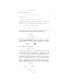
For examples of flavors of gwffs, see page 41.
CHAPTER 3
Top-Levels
1. Defining a Top Level
Top levels are a Tps3 category, whose definition is given in section 2.
For an example, let’s look at the editor top level:
(deftoplevel ed-top
(top-prompt-fn ed-top-prompt)
(command-interpreter ed-command-interpreter)
(print-* ed-print-*)
(top-level-category edop)
(top-level-ctree ed-command-ctree)
(top-cmd-decode opdecode)
(mhelp "The top level of the formula editor."))
This says that the top level ed-top identifies itself by the function
ed-top-prompt, which is one of the more complicated prompt functions in
Tps3 ; its only purpose is to print the <ed34> messages at the start of each
line in the editor, but the complications are necessary because the editor can
be entered recursively.
The next line of the toplevel definition gives the name of the command
interpreter function. The print-* function is a function that gets called
after every line; in this case, it’s the ed-print-* function, which prints out
the current wff if it has changed due to the last command. The top level
category is edop, which is defined as follows:
(defcategory edop
(define defedop)
(properties
(alias single)
(result-> singlefn)
(edwff-argname single)
(defaultfns multiplefns)
(move-fn singlefn)
(mhelp single))
(global-list global-edoplist)
(shadow t)
(mhelp-line "editor command")
(scribe-one-fn
(lambda (item)
25
26
3. TOP-LEVELS
(maint::scribe-doc-command
(format nil "@IndexEdop(~A)" (symbol-name item))
(remove (get item ’edwff-argname)
(get (get item ’alias) ’argnames))
(or (cdr (assoc ’edop (get item ’mhelp)))
(cdr (assoc ’wffop (get (get item ’alias) ’mhelp)))))))
(mhelp-fn edop-mhelp)))
This category defines the sort of command found in the editor top level
(compare the above definition with that of mexpr, for example). So all the
commands that can only be seen from the editor top level are defined with
the defedop command, as follows:
(defedop o
(alias invert-printedtflag)
(mhelp "Invert PRINTEDTFLAG, that is switch automatic recording of wffs
in a file either on or off. When switching on, the current wff will be
written to the PRINTEDTFILE. Notice that the resulting file will be in
Scribe format; if you want something you can reload into TPS, then use
the SAVE command."))
The top-command-ctree is used for command completion, and the mhelp
property is obvious. This leaves top-cmd-decode, which is the name of the
function that is called by the command interpreter to, for example, fill in
the default arguments for an edop.
2. Command Interpreters
Each top level has its own command interpreter. The actual command
interpreters in much of the code are older versions; the code has since been
simplified considerably. New command interpreters, which may in time replace the older versions, and which should certainly be used as the models
for the command interpreters of any new top levels, are in the two files
command-interpreters-core.lisp and command-interpreters-auto.lisp.
CHAPTER 4
MExpr’s
Tps3 provides its own top-level. It allows for default arguments and
provides a way of giving arguments (e.g. wffs) in some external representation which is converted before the "real" function is called. All this is
also available in an interactive mode, where the user is prompted for arguments after he has been told what the defaults are and which alternatives
are open. The way all this has been implemented is through MExpr’s, which
constitute special functional objects analogous to Expr’s or FExpr’s in LISP.
Every Tps3 command should be an MExpr so that the facilities of Tps3 ’
top-level can be utilized.
1. Defining MExpr’s
Mexprs are special functional objects that are recognized by the top level
of Tps3. They can be defined with the defmexpr macro, which has a number
of optional arguments. The general format is ( indicate optional arguments)
(defmexpr {\it name}
{(ArgTypes {\it type1} {\it type2} ...)}
{(ArgNames {\it name1} {\it name2} ...)}
{(ArgHelp {\it help1} {\it help2} ...)}
{(DefaultFns {\it fnspec1} {\it fnspec2} ...)}
{(EnterFns {\it fnspec1} {\it fnspec2} ...)}
{(MainFns {\it fnspec1} {\it fnspec2} ...)}
{(CloseFns {\it fnspec1} {\it fnspec2} ...)}
{(Print-Command {\it boolean})}
{(Dont-Restore {\it boolean})}
{(MHelp "{\it comment}")}
There are actually two other possible entries, Wffop-Typelist and WffArgTypes;
these are only used in mexprs which are generated automatically by the Rules
package.
In the following a function specification is either a symbol naming a
function, or an expression of the form (Lambda arglist . body). We also
assume that the main function which is to perform the command has n
arguments. Then the phrases in the above definition have the following
meaning.
name: This is the name of the MExpr as called by the user.
27
28
4. MEXPR’S
ArgTypes: This is a list which must have as many elements as the
function arguments, i.e. n. type1, type2, ..., typen have to be valid
types, which means that they have to have a non-NIL ArgType property. Each argument supplied by the user on the command line will
be processed first by the corresponding GetFn. In case an FExpr is
to be called, each element of the argument list is presupposed to be
of the same type. This type is specified in parentheses. If ArgTypes
is omitted, the function has no arguments.
ArgHelp: This has to be a list of length n. Each element is a string
describing the argument, or NIL. These quick helps for arguments
can be accessed via the ? when being prompted for the argument
value. For an FExpr, there should be only one string.
DefaultFns: The fnspecs declared in this place are being processed
in a left-to-right order, where the result of one fnspec is passed on
to next. A fnspec can signal an error (a THROW with a FAIL label) if
the arguments seem to be contradictory (e.g. if a planned line and
a term is supplied for a P-rule, but the term does not appear in the
proof), but it can count on the arguments being of the correct type
and in internal representation.
In detail, each default fnspec must be either a symbol denoting a
function of n arguments, where n is the number of mexpr arguments,
or else a lambda expression of n arguments. Each fnspec must return
a list of length n. This list will then be handed on and processed
by the next fnspec as if it were the list of arguments supplied by
the user. Any entry which is not a $ should be left unchanged. The
function is not allowed to have side-effects. As a general convention,
the arguments which are not used by a fnspec are not written out
with their name, but replaced by %i. This makes it easier to see at
one glance which defaults are filled in by a certain defaultspec.
EnterFns: fnspec1, fnspec2, ... is an arbitrary list of function specifications. They are called in succession with the value list returned
by the last default fnspec, before the MainFns are called.
MainFns: fnspec1, fnspec2, ... is an arbitrary list of function specifications. They are called in succession with the value list returned by
the last default fnspec. If none are specified, it is assumed that there
is a function named name, which can be called. Notice that at this
stage, no defaulted arguments may be left. ComDeCode (the command processing function) will refuse to call any function, unless all
the defaults are determined. This clearly divides the responsibilities
between GetFn’s, DefaultFn’s and MainFn’s. Any fnspec may abort
with an error by doing a THROW with a FAIL label. A THROW with a
TryNext label will be handled like a normal return. A THROW with
a CutShort label means that none of the remaining MainFn’s will
be executed and the value of the THROW will be handed on to the
CloseFn’s.
2. ARGUMENT TYPES
29
CloseFns: fnspec1, fnspec2, ... is a list of function specifications.
They are called in succession with the value returned by the last
MainFn. Even if the MainFn’s were FExpr’s, each fnspec has to
describe an Expr.
Dont-Restore: boolean determines whether or not this command will
be restored, if it is saved using SAVE-WORK. For example, commands like HELP and ? should not be restored.
Print-Command: boolean is used by RESTORE-WORK and EXECUTEFILE, which both ask "Execute Print-Commands?"; this is how
they know which commands are print commands.
MHelp: This has to be a string and will be available through UserHelp
and the ?? if no QuickHelp is available.
2. Argument Types
At the top-level of Tps3 explicitly declared argument types are available.
Many of the more important ones are all declared in the file argtyp.lisp.
They can be recognized by their ArgType property value, which is T. Each
of argument type has at least three properties, GetFn, TestFn, and PrintFn.
GetFn is responsible for translating the user’s value into internal representation, TestFn tests if some object is of the given type, and PrintFn makes
the internal representation intelligible to the user.
The defining command for the category argtype is actually deftype%%,
but all definitions of argtypes should be made through the secondary macro
DefType%. Its format is as follows ( enclose optional arguments):
(DefType% {\it name}
(GetFn {\it fnspec})
(TestFn {\it fnspec})
(PrintFn {\it fnspec})
{(Short-Prompt {\it boolean})}
{(MHelp "{\it comment}")}
{({\it property1} {\it value1}) ({\it property2} {\it value2}) ...})
In the above a fnspec is either the name of a one-argument function, or a list
of forms which are to be evaluated as an implicit progn. In the latter case,
name stands for the argument supplied.
name: The name of the argument type. It will get a property value of
T for the property ArgType when the DefType% has been executed.
GetFn: Here fnspec defines the function used to process the argument
as supplied by the user on the command line. The value returned
by it is then handed on to the main function executing the command. No GetFn will ever receive a $. It is simply not called, if
the corresponding argument in the command line is defaulted. A
GetFn should signal an error if the argument is not of the correct
type. This will be implemented (as it is right now) as a THROW with
the label FAIL. A special case of fnspec for a GetFn is TestFn. This
30
4. MEXPR’S
means the GetFn will test if the supplied argument is of the correct
type. If yes, the argument will simply be returned, otherwise an
error will be signaled. A GetFn may have side-effects, but this has
to be declared under Side-Effects.
PrintFn: Here fnspec should print the external representation of its
only argument. It can expect this argument to be of the correct
type. The value returned is ignored. A PrintFn may signal an
error if printing is not possible (e.g. if the current style does not
have a representation of the given data type).
TestFn: Here fnspec should return NIL if its argument is not of type
name, and return something not NIL otherwise.
Short-Prompt: boolean is only used in otl-typ.lisp, but I can’t work
out what for.
MHelp: This is an optional documentation and is accessed during
MHelp or after a ? while the user supplies command arguments
interactively.
(property value): Pairs like this allow for more information about the
type. 1
For example
(deftype% anything
(getfn (lambda (anything) anything))
(testfn (lambda (anything) (declare (ignore anything)) t))
(printfn princ)
(mhelp "Any legal LISP object."))
(deftype% integer+
(getfn testfn)
(testfn (and (integerp integer+) (> integer+ -1)))
(printfn princ)
(mhelp "A nonnegative integer."))
(deftype% boolean
(getfn (cond (boolean t) (t nil)))
(testfn (or (eq boolean t) (eq boolean nil)))
(printfn (if boolean (princ t) (princ nil)))
(mhelp "A Boolean value (NIL for false, T for true)."))
No TestFn or PrintFn is allowed to have any side-effects, since they may
be called arbitrarily often. No GetFn needs to expect $ as an argument,
since defaults are now figured out elsewhere. This avoids conflicts between
different defaults for the same argument type in different functions. Hence
GetFn never computes the default.
1More properties may become useful, so the Deftype% macro allows arbitrary property
names. Possibilities here include EdFn (for editing this argument type) or OutputFn (to
be able to read back a data object of the specified type.)
2. ARGUMENT TYPES
31
2.1. List Types. The macro deflisttype defines a list from an existing type:
(deflisttype filespeclist filespec)
This takes an existing type, filespec, and produces a type of lists of
filespecs. It is also possible to specify other properties (the same properties
as for deftype%), in which case these properties override those of the original
type. This is typically used to give the list type a different help message from
the original type.
2.2. Consed Types. The macro defconstype defines a type as a cons
of two existing types:
(defconstype subst-pair gvar gwff
(mhelp "Means substitute gwff for gvar."))
This takes two existing types, gvar and gwff, and produces a type
subst-pair of consed pairs (gvar . gwff). It is also possible to specify other properties (the same properties as for deftype%), in which case
these properties override those of the original type. This is typically used to
give the cons type a different help message from the original type.
CHAPTER 5
Representing Well-formed formulae
1. Types
typeconstant : ::= Type Constant
An identifier with a non-NIL TypeConst property. For example,
O and I:
(def-typeconst o
(mhelp "The type of truth values."))
typevariable : ::= Type Variable
An identifier with a non-NIL TypeVar property.
It is the parsers responsibility to give the TypeVar property to types not
previously encountered.
typesymbol : ::= typeconstant | typevariable | (typesymbol .
bol)
typesym-
2. Terminal Objects of the Syntax
Before going into detail about the terminal objects of the syntax, some
general remarks about type polymorphism in Tps3 are needed.
Tps3 supports polymorphic objects, like ⊆ (subset), which is a relation
that may hold between sets of any type. It must be understood, however,
that the parser completely eliminates this ambiguity of types, when actually
reading a wff. In a given wff every proper subwff has a type! Therefore,
there is a class of objects with polymorphic type, which never appear in
a wff, but nevertheless may be typed by the user. The instances of those
polymorphic abbreviations or polymorphic proper symbols inside the formula
will refer, however, to those polymorphic primitive symbols or polymorphic
abbreviating symbols.
For reasons of efficiency, binders are handled slightly differently. Binders
are also polymorphic in the sense that a certain binder, say ∀, may bind
variables of any type. The case of binder, however, is slightly different from
that of polymorphic abbreviations, since a binder is not a proper subwff.
Binders, therefore, are left without having a proper type. We must, however,
be able to figure out the type of any given bound wff. Thus each binder
carries the information about the type of the scope, the bound variable and
the resulting bound wff with it. See Section 5 for more details.
33
34
5. REPRESENTING WELL-FORMED FORMULAE
The list below introduces syntactic categories of objects known to the
parser only, which are not legal in wffs themselves.
pmprsym : ::= Polymorphic Primitive Symbol
pmprsyms are the STANDS-FOR property of pmpropsyms, but
cannot appear in gwffs themselves. Examples would be PI or IOTA.
pmabbsym : ::= Polymorphic Abbreviating Symbol
pmabbsym are the STANDS-FOR property of pmabbrevs, but cannot appear in gwffs themselves. Examples are SUBSET, UNION, or
IMAGE.
The following categories are the “terminal” objects of proper wffs. The
parser may not produce a formula with any other atomic (in the Lisp sense)
object then from the list below.
logconst : ::= Logical Constants
For example: AND, OR, IMPLIES, NOT, FALSEHOOD, TRUTH:
(def-logconst and
(type "OOO")
(printnotype t)
(infix 5)
(prt-associative t)
(fo-single-symbol and)
(mhelp "Denotes conjunction."))
propsym : ::= Proper Symbols
For example: P<OA>, x<A>, y<A>, Q<OB>, x<B> are proper symbols after parsing ∀ x∀ y. Poαα x y ∧ Qoα x. This example demonstrates part of the parser. Since in a given wff, a proper symbol
may appear with more than one type, the type of each proper must
somehow be encoded in its name. Tps3 does this by appending the
type, ( and ) replaced by < and >, respectively, to the print name
of the symbol.
pmpropsym : ::= Polymorphic Proper Symbols
These are just like propsym, except that they also have a STANDS-FOR
property, which is the polymorphic primitive symbol (pmprsym)
this polymorphic proper symbol was constructed from. Note that
this particular instance of the polymorphic primitive symbol always
has a specific given type. For example: IOTA<I<OI» is a pmpropsym
after parsing yι = ι[QQy]:
(def-pmpropsym iota
(type "A(OA)")
(typelist ("A"))
(printnotype t)
(fo-single-symbol iota)
(mhelp "Description operator"))
abbrev : ::= Abbreviations
2. TERMINAL OBJECTS OF THE SYNTAX
35
For example: @EQUIV. This is separate category from polymorphic abbreviations only for reasons of efficiency. An abbreviation could be thought of as a polymorphic abbreviation with an
empty list of type variables. For example:
(def-abbrev equiv
(type "OOO")
(printnotype t)
(fo-single-symbol equiv)
(infix 2)
(defn "[=(OOO)]"))
pmabbrev : ::= Polymorphic Abbreviations
For example: SUBSET<O<OA><OA», SUBSET<O<OB><OB» are polymorphic abbreviations after parsing A@f12(oa) @SUBSET B @or
[R@f12(obb) a] @ @SUBSET [R b]. For example:
(def-abbrev subset
(type "O(OA)(OA)")
(typelist ("A"))
(printnotype t)
(infix 8)
(fo-single-symbol subset)
(defn "lambda P(OA) lambda R(OA). forall x . P x implies R x"))
binder : ::= Variable Binders
For example: ∀, ∃, λ, ∃1 . See the section below.
label : ::= A Label referring to one or more other wffs.
For example: AXIOM1, ATM15, LABEL6. See Section 6.
In principle, the implementation is completely free to choose the representation of the different terminal objects of the syntax. The functions with
test whether a given terminal object is of a given kind is the only user visible
functions. Once defined, the particular implementation of the object should
not be needed or relied upon by other functions.
It is explained more precisely what is meant by “quick” and “slow” predicates to decide whether a given object is in a certain syntactic category
in section 1.5. Here is a table of the different syntactic categories with the
“slow” test function for it and the properties that are required or must be
absent. Keep in mind that the list reflects the current implementation, and
may not be reliable.
36
5. REPRESENTING WELL-FORMED FORMULAE
Category
Predicate
Required Properties
Absent Properties
pmprsym
PMPRSYM-P
pmabbsym
PMABBSYM-P
TYPE, TYPELIST
DEFN
TYPE, TYPELIST, DEFN
logconst
propsym
LOGCONST-P
PROPSYM-P
pmabb
PMPROPSYM-P TYPE, POLYTYPELIST, STANDS-FOR (a pmabbsym)
abbrev
ABBREV-P
label
LABEL-P
TYPE, DEFN
TYPELIST
FLAVOR
binder
BINDER-P
VAR-TYPE, SCOPE-TYPE, WFF-TYPE
TYPE, LOGCONST
TYPE
LOGCONST, STANDS-FOR
pmpropsym PMPROPSYM-P TYPE, POLYTYPELIST, STANDS-FOR (a pmprsym)
3. Explanation of Properties
The various properties mentioned above are as follows:
TYPE : The type of the object. Common are "OOO" for binary connectives and "I" for individual constants.
PRINTNOTYPE : In first-order mode, this is insignificant, but if specified
and T, Tps3 will never print types following the object. It is almost
always appropriate to specify this.
INFIX : The binding priority of an infix operator. This will declare
the connective to be infix. The absolute value of INFIX is irrelevant, only the relative precedence of the infix and prefix operators
matters. If two binders have identical precedence, association will
be to the left. For example, if R1 and R2 are operators with INFIX
equal to 1 and 2, respectively, "p R1 q R2 r R2 s" will parse as
"[p R1 [[q R2 r] R2 s]]".
PREFIX : The binding priority of a prefix operator. Binders are considered prefix operators (see about binders below) and thus have a
binding priority. The main purpose of a prefix binding priority is
to allow formulas like " a=b" to be parsed correctly as " [a = b]"
by giving = precedence over .
PRT-ASSOCIATIVE : indicates whether to assume that the operator is
left associative during printing. You may want to switch this off
(specify NIL) for an infix operator like equivalence, say <=>, since
3. EXPLANATION OF PROPERTIES
37
"p <=> q <=> r" is often considered to mean "p <=> q & q <=>
r".
FO-SINGLE-SYMBOL : this is meaningful only in first-order mode and
declares the object to be a “keyword” in the sense that it may be
typed in all upper or lower case. Moreover, the printer will surround
it by blanks if necessary to set off surrounding text. Also the parser
will expect that the symbol is delimited by spaces, dots, brackets,
unless the symbol just consists of one letter, in which case it doesn’t
matter. You MUST use this attribute in first-order mode for an
identifier with more than one character.
MHELP : An optional help string.
Properties specific to binders are described in the section below about
binders. Here are some more examples. These examples do not actually
exist under these names in Tps3.
(def-logconst &
(type "OOO")
(printnotype t)
(infix 5)
(prt-associative t)
(fo-single-symbol &)
(mhelp "Conjunction."))
Note that the (fo-single-symbol &) will make sure that spaces are
printed around & in formulas.
In the next example the character / is used to make sure that the disjunction is printed in lowercase, that is as v instead of V.
(def-logconst /v
(type "OOO")
(printnotype t)
(infix 4)
(prt-associative t)
(fo-single-symbol /v)
(mhelp "Disjunction."))
(def-logconst =>
(type "OOO")
(printnotype t)
(infix 3)
(fo-single-symbol =>)
(mhelp "Implication."))
We do not like spaces after negation. So we do not declare it to be a
fo-single-symbol. That works only because - consists of only one character.
(def-logconst (type "OO")
38
5. REPRESENTING WELL-FORMED FORMULAE
(printnotype t)
(prefix 6)
(mhelp "Negation."))
4. Non-terminal Objects of the Syntax
[lsymbol] ::= logconst
| propsym
| pmpropsym
| abbrev
| pmabbrev
lsymbol roughly corresponds to what was called hatom for Huet-atom
from Huet’s unification algorithm in the old representation.
Generalized WFFs
gwff ::= lsymbol
| ((propsym . binder) . gwff) ; Generalized binder
| (gwff1 . gwff2) where (cdr (type gwff1)) = (type gwff2)
| label
5. Binders in TPS
In the discussion about the internal representation of wffs the issue of
binders has been neglected so far. Currently, TPS allows three binders, λ,
∀, ∃ (plus some “buggy” fragments of support for the ∃1 binder).
Since most binders are inherently polymorphic, there is only one kind of
binder. Notice that the definition is formulated such that a binder may have
a definition, but need not.
In order to determine the type of a bound wff, the type of the scope
of the binder must be matched against the type stored in the SCOPE-TYPE
property. Also, the type of the bound variable must match the type in the
VAR-TYPE property. These matches are performed, keeping in mind that all
types in the TYPELIST property are considered to be variables. Then the
bindings established during the match are used to construct the type of the
whole bound wff, using the WFF-TYPE property of the binder.
An example may illustrate this process. The binder LAMBDA has the
following properties
TYPELIST
(A B)
VAR-TYPE
B
SCOPE-TYPE A
WFF-TYPE
(A . B)
When trying to determine the type of λxι .Roιι x, Tps3 determines that
A must be ι, and that B must be oι. The type of the original formula is (A .
B) which then turns out to be oιι.
Note that TYPELIST may be absent, i.e. could be (), which amounts to
stating that the binder has no variable types. Currently, we are not using
5. BINDERS IN TPS
39
such binders. An example would be Foralln , which can bind only variables
of type σ.
In addition to the properties mentioned above, a binder (except λ) would
have a definition. One can then instantiate a binder just as a definition can
be instantiated. The definition is to be written with two designated variables,
one for the bound variable and one for the scope. For example THAT has
definition
ια(oα) .λbα So
Here the TypeList would be (α), designation for the bound variable would
be bα , designation for the scope would be So .
The internal representation for a binder inside a wff is always the same
and simply ((bdvar . binder) . scope), but all of the above information must be present to determine the type of a wff, or to check whether
formulas are well-formed.
Fancy “special effects” such as ∀x ∈ S.A must be handled via special
flavors of labels and are not treated as proper binders themselves.
Here are some examples of binders:
(def-binder lambda
(typelist ("A" "B"))
(var-type "A")
(scope-type "B")
(wff-type "BA")
(prefix 100)
(fo-single-symbol lambda)
(mhelp "Church’s lambda binder."))
(def-binder forall
(typelist ())
(var-type "I")
(scope-type "O")
(wff-type "O")
(prefix 100)
(fo-single-symbol forall)
(mhelp "Universal quantifier."))
{\it The above definition is for math-logic-1, where forall can only bind individual
variables. In math-logic-2, the definition is as follows:}
(def-binder forall
(typelist ("A"))
(var-type "A")
(scope-type "O")
(wff-type "O")
(prefix 100)
40
5. REPRESENTING WELL-FORMED FORMULAE
(fo-single-symbol forall)
(mhelp "Universal quantifier."))
5.1. An example: How to See the Wff Representations. You
can see examples of how wffs are represented by comparing the output of
the editor commands P and edwff:
<44>ed x2106
<Ed45>p
FORALL x(I) [R(OI) x IMPLIES P(OI) x] AND FORALL x [~Q(OI) x IMPLIES R x]
IMPLIES FORALL x.P x OR Q x
<Ed46>edwff
((IMPLIES (AND (|x<I>| . FORALL) (IMPLIES R<OI> . |x<I>|) P<OI> . |x<I>|)
(|x<I>| . FORALL) (IMPLIES NOT Q<OI> . |x<I>|) R<OI> . |x<I>|)
(|x<I>| . FORALL) (OR P<OI> . |x<I>|) Q<OI> . |x<I>|)
Another way to do this is as follows:
<3>ed x2106
<Ed4>cw
LABEL (SYMBOL): [No Default]>x2106a
<Ed5>(plist ’x2106a)
(REPRESENTS ((IMPLIES (AND (|x<I>| . FORALL) (IMPLIES R<OI> . |x<I>|)
P<OI> . |x<I>|) (|x<I>| . FORALL) (IMPLIES NOT Q<OI> . |x<I>|) R<OI> . |x<I>|)
(|x<I>| . FORALL) (OR P<OI> . |x<I>|) Q<OI> . |x<I>|) FLAVOR WEAK)
And another way:
<2>(getwff-subtype ’gwff-p ’x2106)
((IMPLIES (AND (|x<I>| . FORALL)
(IMPLIES R<OI> . |x<I>|) P<OI> . |x<I>|) (|x<I>| . FORALL)
(IMPLIES NOT Q<OI> . |x<I>|) R<OI> . |x<I>|)
(|x<I>| . FORALL) (OR P<OI> . |x<I>|) Q<OI> . |x<I>|)
And finally a way that only works at type O (the 0 below is a zero, not
a capital O):
<3>(get-gwff0 ’x2106)
((IMPLIES (AND (|x<I>| . FORALL)
(IMPLIES R<OI> . |x<I>|) P<OI> . |x<I>|)
(|x<I>| . FORALL)
(IMPLIES NOT Q<OI> . |x<I>|) R<OI> . |x<I>|)
(|x<I>| . FORALL)
(OR P<OI> . |x<I>|) Q<OI> . |x<I>|)
6. FLAVORS AND LABELS OF GWFFS
41
6. Flavors and Labels of Gwffs
It is sometimes desirable to be able to endow a gwff with additional
properties. For example, one may wish to be able to refer to a gwff by a short
tag, or to specify that a particular gwff is actually a node in an expansion
tree. For this purpose, Tps3 provides the facility of labels and flavors (see
page 23). A label is an object which, as far as Tps3 is concerned, is merely
a special case of gwff. Labels thus stand for gwffs, but may have additional
properties and distinct representations.
Flavors are the classes into which labels are divided. The definition of
a flavor specifies some common properties of a class of labels, usually the
behavior of wffops and predicates. Also, a flavor’s definition should specify
what attributes each label of that flavor should have, and how it should be
printed.
6.1. Representation. Each flavor is represented in Tps3 by a Lisp
structure of type flavor, which has the following slots: wffop-hash-table,
which stores the properties common to each instance of the flavor, in particular, how wffops are to behave; constructor-fun, which is the name of
the function to be called when a new label of the flavor is to be created;
name, the flavor’s name; and mhelp, a description of the flavor. The values
of these slots are automatically computed when Tps3 reads a defflavor
declaration. The flavor structures are stored in a central hash table, called
*flavor-hash-table*, keyed on the flavor names. This also is updated
automatically whenever a flavor is defined (or redefined).
There are two ways to represent labels (instances of flavors), and the
choice is made during the definition of the flavor. The first, and more traditional, way is to have each label be a Lisp symbol, with the attributes of the
label being kept on the symbol’s property list. The second way is to make
each label a Lisp structure. The type of the structure is the name of the
flavor; thus an object’s type can be used to determine that it is a label of a
certain flavor.
If one wishes to have labels be symbols, nothing must be done; this is
the default. A flavor’s labels will be structures only if one of two things
is declared in the defflavor. The first is that the property structured
appears. The second is if another flavor whose instances are structures is
specified to be included in the new flavor.
When a flavor’s labels are to be structures, one will usually wish to
specify the printfn property so that the labels will be printed in a nice way.
This function must be one which is acceptable for use in a defstruct. It is
also required that one specify the slots, or attributes, the structures are to
have, by including a list of the form
(instance-attributes (slot1 default1) ... (slotN defaultN))
in the flavor definition.
42
5. REPRESENTING WELL-FORMED FORMULAE
6.2. Using Labels. The function define-label is a generic way to
create new labels of a specified flavor. The function call (define-label
sym flavor-name) will do one of two things. If flavor-name is a flavor
whose labels are symbols, then the property list of sym will be updated
with property FLAVOR having value flavor-name. If on the other hand,
flavor-name is a flavor having structures for labels, then sym will be setq’d
to the value of the result of calling the constructor function for flavor-name,
which will create a structure of type flavor-name.
To access the attributes of a label which is a symbol, use get, since
all attributes will be on the symbol’s property list. The attributes of a
label which is a structure of type flavor-name can be accessed by using
the standard Lisp accessing functions for structures. Thus, if one of the
label’s attributes is represents, the attribute can be accessed by calling the
function flavor-name-represents.
Flavors can be redefined or modified at any time. This may be done if, for
example, one wished to extend a flavor’s definition into a Lisp package which
was not always loaded. Merely put another defflavor statement into the
code. You need only put the new or changed properties in the redefinition.
If, however, you wish to change the attributes of a flavor which is a structure,
you should put in all of the attributes you desire, not just the new ones, and
be sure to declare any included flavor as well. Note: it is possible to change
a flavor which uses symbols as labels into one which uses structures, but if
you fail to redefine code which depends on property lists, the program will
be smashed to flinders.
6.3. Inheritance and Subflavors. Some flavors may be similar in
many ways; in fact, some flavors may be more specialized versions of other
flavors. One may wish a new flavor’s labels to be operated upon by most
wffops in the same way as an existing flavor’s labels; this we will call inheritance of properties. In addition, one may wish a new flavor to actually be
a subtype (in Lisp terms) of an existing flavor, and have the attributes of
the existing flavor’s labels be included in the attributes of the new flavor’s
labels; this we will call inclusion of attributes. The defflavor form allows
either or both types of sharing to be used.
Inheritance of properties is signalled in the defflavor by a form such
as (inherit-properties existing-flavor1 ... existing-flavorN). This will
cause the properties in the wffop-hash-table of the existing flavors to be
placed into the wffop-hash-table of the new flavor. If any conflict of properties occurs, e.g., if existing-flavorI and existing-flavorJ, I < J, have a property with the same name, then the value which existing-flavorJ has for that
property will be the one inherited by the new flavor. A new flavor may
inherit properties from any number of existing flavors.
In contrast, attributes may be included from only one other flavor. This
can be done by using the form (include existing-flavor). The existing flavor must be a flavor whose instances are structures, and the new flavor’s
6. FLAVORS AND LABELS OF GWFFS
43
instances will also be structures whose slots include the attributes of the
existing flavor. Thus the same accessing functions for those slots will work
on labels of both flavors. To define default values for those slots, add them
to the include form as if it were an :include specifier to a defstruct; e.g.,
(include existing-flavor (slot1 default1)).
6.4. Examples. Here are some examples of flavor definitions.
(defflavor etree
(mhelp "Defines common properties of expansion tree nodes.")
(structured t)
(instance-attributes
(name ’|| :type symbol)
components ; a node’s children
(positive nil ) ; true if node is positive in the
;formula
(junctive nil :type symbol) ; whether node acts as neutral,
;conjunction, or disjunction
free-vars ; expansion variables in whose scope
; node occurs,
; used for skolemizing
parent ; parent of the node
;;to keep track of nodes from which this node originated when copying a
;;subtree
(predecessor nil)
(status 1))
(printfn print-etree)
(printwff (lambda (wff bracket depth)
(if print-nodenames (pp-symbol-space (etree-name wff))
(printwff
(if print-deep (get-deep wff)
(get-shallow wff))
bracket depth))))
...many more properties...)
Etree labels will be structures, with several attributes. The function
used to print them will be print-etree.
(defflavor leaf
(mhelp "A leaf label stands for a leaf node of an etree.")
(inherit-properties etree)
(instance-attributes
shallow)
(include etree (name (intern-str (create-namestring leaf-name))))))
Leaf labels will also be structures, with attributes including those of
etree, as well as a new one called shallow. Note that the name attribute is
given a default in the include form. Leaf inherits all of the properties of
44
5. REPRESENTING WELL-FORMED FORMULAE
etree, including, for example, its print function, unless they are explicitly
redefined in the definition of leaf.
CHAPTER 6
Printing and Reading Well-formed formulas
1. Parsing
Frank has implemented a type inference mechanism based on an algorithm by Milner as modified by Dan Leivant. Type inference is very local:
The same variable, say "x" will get different type variables assigned, when
used in different formulas. Since multiple use of names with different types is
rare, the default could be changed, so that after the first occurrence of an "x"
during a session core image, the type inferred the first time is remembered.
There are only a total of 26 type variables, so you may run out during a
session. The function INITTYPES reset the way type variables are assigned
and treats everything except O and I as type variables. Normally, a type
variable once mentioned or assigned automatically becomes a type constant.
If TYPE-IOTA-MODE is NIL, then TPS will assign type variables starting with Z and going backwards, as more are needed. TYPE-IOTA-MODE
defaults to T.
Polymorphic abbreviations like SUBSET now may be given a type, so
as to fix the type of other variables. E.g. the following is legal: "FORALL
x . P x IMPLIES [Q x] IMPLIES . P SUBSET(O(OC)(OC)) Q" Note that
"x" will be typed "C" (Gamma). The same typing could have been achieved
by "FORALL x(C) . P x IMPLIES [Q x] IMPLIES . P SUBSET Q" If all
the types were omitted and TYPE-IOTA-MODE were NIL, "x" would have
been typed with the next available typevariable.
Using the same name for two variables of distinct type is legal, but not
recommended. Consider, for example, "FORALL x . P x(I) AND . Q . x(II)
a" Here the type of the very first occurrence of "x" will be assumed as "II".
Leaving out the type of the third occurrence of "x" would have led to an error
message: Rather than assume that "x(II)" was really meant, TPS assumes
instead that the scoping must have been incorrect, which seems much more
likely.
All remaining type variables (after a parse) are automatically assumed
to be of base-type unless the flag TYPE-IOTA-MODE is set in which case they
are assumed to be of type ι. In first-order mode identifiers have only single
characters (Thus "not Pxy" is parsed as "NOT . P x y").
When a wff is read in and parsed, each input token (where the number
of characters in a token is dependent on whether you are reading in firstorder-mode or not) is made into a lisp symbol which incorporates the token’s
45
46
6. PRINTING AND READING WELL-FORMED FORMULAS
printed representation and type. For example, entering "x(A)" will result in
a symbol being created whose print-name is "x<A>". When you try to print
a symbol like this, first the part without the type information is printed, then
the type (if necessary) is printed. E.g., first we print "x", then print "(A)".
But the information necessary to print "x" is really on the property list of
the symbol whose print-name is "x". So all wffs of the form "x<...>" will
be printed the same way (except for the type).
So, if you enter "x1(A)", you get the symbol "x1<A>", but no information about a superscript is put on the symbol "x1". Thus when you print
it, you get no superscript, just "x1". Where do superscripts come from,
then? Well, when TPS renames a variable in order to get a new one (such
as alpha-normalizing a wff), it puts the superscript information on the new
symbol’s property list. I.e., if we rename "x1<A>", we may get the symbol
"x2<A>", and on the property list of "x2", we get the superscript information. Thus, the next time the user types in "x2(A)" or even "x2(I)", the
symbols created will have the superscript information.
This can be a little confusing, because the "x1(A)" that you originally
entered still isn’t superscripted, but the renamed variables "x2", "x3", etc.,
will be.
2. Printing of formulas
2.1. The Basics. In this section we will talk about how a formula in
internal representation is printed on different output devices. There are two
main points to take into consideration: how will the parts of the formula
appear, and where will they appear. For the latter refer to section 3, the
former we will discuss now.
2.2. Prefix and Infix. Since we deal with formulas of type theory, we
can regard every formula as built by application and λ-abstraction from a
few primitives. In order to make formulas more legible and closer to the form
usually used to represent formulas from first order logic, we furthermore have
quantification and definitions internally, and quantification, definitions, and
infix operators for the purpose of input and output.
The application of a function to an argument is printed by simply juxtaposing the function and its argument. As customary in type theory, we
do not have an explicit notation for functions of more than one argument.
Predicates are represented as functions with truth values as their codomain.
Infix operators have to be declared as such. Only conjunction, disjunction, and implication are automatically declared to be infix operators. In
general, infix operators will be associated to the left, if explicit brackets are
missing. For example
A ∧ B ∧ C will be [[A ∧ B] ∧ C]
Internally every infix operator has a property Infix which is a number. This
number is the relative binding strength of this infix operator. You will have
2. PRINTING OF FORMULAS
47
to specify it, if you define a new connective to be infix. The higher the priority, the stronger the binding. As usual, ‘∧’ binds stronger than ‘∨’ which
has precedence over ‘⊃’ (implication).
(As an aside, if you don’t want conjunctions bound more tightly than
disjunctions, but want brackets to appear, make the INFIX property of OR
the same as AND. Thus, do: (GET ’AND ’INFIX), to find it is 5, and then
(PUTPROP ’OR 5 ’INFIX))
Unfortunately prefix operators like negation, do not currently have a
binding strength associated with them and will always be associated to the
left. This has to be kept in mind, when formulas are typed in.
Definitions can be infix or prefix and the same rules hold for them.
There are flags which control whether a definition or its instantiation will be
printed. Similarly, logical atoms can appear as names or as values (or both).
In general the appearance of a formula and in particular of a definition very
much depends on which output device is used. See section 2.5 for more detail, but remember that this only affects the way the primitive or defined
symbols appear, but not how the formula is assembled from its parts.
2.3. Parameters and Flags. The flags listed below are global parameters which can be set by the user to control the way formulas are printed.
These settings can be overridden if specific commands are given.
PrintTypes: = T causes all types to be printed. If a typed symbol
occurs more than once, only the first occurrence will have a type
symbol, unless the same symbol name appears in the same formula
with a different type.
= NIL suppresses type symbols.
PrintDepth: This is a parameter which determines how deep the
recursion which prints the formula will go. Subformulas located at
a lower level will simply be replaced by an &. A PrintDepth of
0 means that everything will be printed, regardless of its depth.
PrintDepth has to be an integer. It is initialized to 0. The most
useful application of this parameter is in the formula-editor, where
one usually does not like to see the whole formula.
AtomValFlag: This flag should usually not be touched by the user.
If it is true, under each atom its value will appear.
AllScopeFlag: This flag should be NIL most of the time. If it is
T brackets and dots will always be inserted, i.e. no convention of
associativity to the left is followed. The precedence values of infix
operators are also ignored. It can be forced to T by calling the
function PWScope GWff.
2.4. Functions available. There are of course a variety of occasions
to print wffs, For example in plans, as lines, after the P or PP -command
in the editor etc. Associated with these are different printing commands
given by the user. Some of these commands override globally set parameters
48
6. PRINTING AND READING WELL-FORMED FORMULAS
or flags. Internally, however, there is only one function which prints wffs.
This function PrtWff is called whenever formulas have to be printed. The
various flags controlling the way printed formulas will appear, will either be
defaulted to the global value, or be passed to this function as arguments.
The general form of a call of PrtWff is as follows
(PrtWff Wff (Parameter1 Value1 ) ... (Parametern Valuen ) )
Before the actual printing is done Parameter1 ... Parametern will be set to
Value1 ... Valuen , resp. If a parameter of the following list is not included in
the call of the function, its global value will be assumed. Possible parameters
with their range and the section they are explained in are
PrintTypes
T,NIL
2.3
PrintDepth
0,1, ...
2.3
AllScopeFlag T,NIL
2.3
AtomValFlag T,NIL
2.3
PPWfflag
T,NIL
3.1
LocalLeftFlag T,NIL
3.1
FilLineFlag
T,NIL
3.1
FlushLeftFlag T,NIL
3.1
Leftmargin
1 ... Rightmargin
2.6
Rightmargin
1, 2 ...
2.6
Style
XTERM, SCRIBE, CONCEPT,
GENERIC, SAIL, TEX ...
2.5
2.5. Styles and Fonts. Tps3 can work with a variety of different output devices, producing special characters like ∀ or ∧ where possible, and
spelling them out (as FORALL and AND) where not. Details of how to produce
output files for various purposes are in the Etps and User’s Manuals.
At no point does the user actually make a commitment whether to work
with special characters or not, since she can easily switch back and forth.
The internal representation is completely independent of these switches in
the external representation.
A few commands, such as VPForm and VPDiag have an argument Style
which specifies the style in which a file is produced. Furthermore there is a
flag, STYLE, which Tps3 will use in the absence of any other indication as
to the appropriate form of output.
Along with the style the user can usually specify an appropriate linelength by using the LEFTMARGIN and RIGHTMARGIN flags. Some commands (most notably SETUP-SLIDE-STYLE) will change both the style
and the default line length.
CONCEPT, CONCEPT-S : this is the style used for a Concept
terminal, which might also occasionally also be useful to produce
a file which can be displayed on the Concept terminal with CAT or
MORE. The difference between CONCEPT and CONCEPT-S is that the
latter assumes that your Concept is equipped with special characters and the former does not. If special characters are available,
2. PRINTING OF FORMULAS
49
you will then get types as greek subscripts, the universal quantifier
as ∀, etc. The default linelength is 80.
GENERIC : this style assumes no special features and defaults the
linelength to 80. For example the existential quantifier shows up as
EXISTS and types are enclosed in parentheses.
GENERIC-STRING : is much like GENERIC, but prints in a format
that can be re-read by Tps3.
SCRIBE : corresponds to the style used by the Scribe text processor. A file produced in this style has to be processed by SCRIBE
before it can be printed. All special characters, superscripts and
subscripts, etc. are available. The main drawback of a SCRIBE-file
is that precise formatting as necessary for vertical path diagrams is
impossible. The font used is 10-point, except when doing SLIDEPROOF, when an 18-point font is used.
TEX : is the output style used by the TEXtext processor. A file
produced in this style has to be processed by TEXbefore it can be
printed. All special characters, superscripts, etc. are available, and
vertical path diagrams are correctly formatted (although often too
wide to print).
XTERM : produces the special characters used by X-windows. You
should set the value of RIGHTMARGIN to reflect the width of the
window containing Tps3.
SAIL : SAIL is a style (now all but obsolete) used for printing on a
Dover printer. The font used is 10-point, with 120 characters per
line in landscape format (used for vertical path diagrams), and 86 in
portrait format (used for all other applications). When you dover
the file , you have to remember size and orientation and specify
it in the switches of your call of DOVER. A SAIL file does not have
subscripts, but has as variety of other special characters.
From the information about the style, the low-level printing functions
determine which sequence of characters, including control characters, to send
to the selected output device. If a symbol expands to a list of known symbols
with different names (e.g. EQUIVS expands to an EQUIV symbol with a
superscript S), then it has a property FACE which contains this information.
Various other properties give the way that the character is to be printed in
different styles. The CFONT property is a pair (KSet . AsciiValue) .
Kset can be 0,1,2, or 3, although currently only the character sets 0, 1,
and 3 are used; this gives the appropriate character for a Concept terminal.
Similarly, the DFONT property is a string "whatever" which will be printed
into Scribe files as @whatever. The TEXNAME property does the same for
the TEXoutput style. There are some special fonts that are declared in the
file tps.mss. A list of the available special characters for the Concept and for
the Dover (in a SCRIBE-file) are explicitly stored in the files cfont.lisp and
dfont.lisp and loaded into Tps3 at the time the system is being built.
50
6. PRINTING AND READING WELL-FORMED FORMULAS
Consider the following example:
SIGMA1 is a binder. It has a property FACE of value (CAPSIGMA SUP1).
CAPSIGMA is a tex special character, a scribe special character, and a
concept special character. It has a property CFONT of value (3 . 83). It has
a property DFONT of value "gS". It has a property TEXNAME of value
"Sigma".
SUP1 is a tex special character, a scribe special character, and a concept
special character. It has a property CFONT of value (1 . 49). It has a property DFONT of value "+1". It has a property TEXNAME of value "sup1".
In a scribe or tex file, or on a Concept with special characters, SIGMA1
will appear as Σ1 ; elsewhere it will be written as SIGMA1. The actual Scribe
output produced will be
@g{S}@\;@^{1}@\;
; the actual TEXoutput will be
\Sigma^{1}
.
2.6. More about Functions. In this section some more details of the
functions which are used to do the printing are given.
As mentioned earlier, the main connection with the rest of Tps3 is the
MACRO PrtWff. It expands into a PROG in which all the parameters given
as arguments are PROG-variables. In the body of the PROG, all parameters are
set to the value specified in the call, then the function PWff is called, just
with Wff as its argument. All the other parameters and flags are now global,
or, in LISP terminology, special variables.
The function PWff performs two main tasks. First a few special variables are set to the correct value. After this is done, PWff checks whether
pretty-printing is desired, i.e. whether PPWfflag is T. For an explanation
of what happens during pretty-printing see section 3 and in particular 3.4.
Otherwise the recursive function PrintWffPlain is called with the appropriate
arguments.
At this point the current style is available to the functions in the flag
STYLE. The calling function has to make sure that LEFTMARGIN and
RIGHTMARGIN will be bound. They are important for the printing functions in order to determine where to break lines, and where to start formulas
on the line. This holds, whether pretty- printing is switched on or off.
Below PWff two functions appear. PrintWffPlain prints a formula without any delimiting symbols around it. For example (with STYLE SCRIBE)
((x<I> . FORALL) . ((OR . (P<OI> . x<I>)) . q<O>)) appears as
∀xι .[Poι x] ∨ qo if BRACKETS = T and as
∀xι [[Poι x] ∨ qo ] if BRACKETS = NIL .
PrintWffScope delimits a composite formula with a preceding dot, if the argument BRACKETS is T , and with brackets around it , if BRACKETS is NIL.
3. PRETTY-PRINTING OF FORMULAS
51
Other than that the functions are identical. In the above example we would
get
∀xι .[Poι x] ∨ qo if Brackets = T and
[∀xι .[Poι x] ∨ qo ] if Brackets = NIL
Both PrintWffPlain and PrintWffScope call PrintWff, where the real work
of distinguishing the different kinds of formulas and symbols is being done.
The distinction between PrintWffPlain and PrintWff is only made for the
sake of pretty-printing (see 3.4).
At an even lower level is the function (actually a macro) PCALL, which
determines the appropriate way to print a particular symbol in the current
style, and prints an error if the relevant function is undefined. PCALL actually
applies to printing functions, rather than characters, so each function will
have a different definition for different styles. For example, in style scribe
the print-symbol function is called PP-SYMBOL-SCRIBE, whereas in style
xterm it’s called PP-SYMBOL-XTERM. (Examine the plists of SCRIBE and
XTERM to verify this, if you like.)
3. Pretty-Printing of Formulas
The most commonly used way of printing formulas, such as lines or
plans, is to pretty-print them. This is a feature quite similar to the way
LISP pretty-prints functions. Formulas which are too long to fit on one line
of the current output device, are broken at the main connective and printed
in several lines. The main difference to the LISP pretty-printing is that we
have to consider infix operators.
The general structure of the functions doing the pretty-printing allows
future changes to the way printing in general is done without making changes
to the pretty-printer. Whenever a formula is to be pretty-printed the usual
printing functions as described above are called, but instead of printing the
characters, they will be appended to a list. Later this list is used to actually
output the characters after the decision where to break the formula has
been made. From this structure it is clear that all the parameters and flags
controlling the appearance of a formula on the several printing devices still
work in the way described before. There are however, a few additional flags
which determine how subformulas will be arranged within a line.
3.1. Parameters and Flags. As new flags particularly for prettyprinting we have
PPWfflag : = T means that formulas will usually be pretty printed.
This is the default value.
= NIL means that formulas never will be pretty printed unless
the command is given explicitly.
LocalLeftFlag : =T will cause the left hand side of an infix expression to be aligned with the operator and not with the right hand
side.
52
6. PRINTING AND READING WELL-FORMED FORMULAS
= NIL is the default and prints left and right hand side of an
infix expression with the same indentation.
FilLineFlag : =T will try to fill a line as much as possible before
starting a new one. This only makes a difference for associative
infix operators.
= NIL starts a new line for each of the arguments of an infix
operator even if only one of several arguments would be too long to
fit on the remainder of the line.
FlushleftFlag : = T switches off indentation completely, i. e. every
line will be aligned with the left margin.
= NIL indents the arguments of infix operators.
3.2. Creating the PPlist. The pretty-printing is achieved in two steps.
During the first phase printing will be done without any formatting and the
characters are not actually printed, but appended to a list, called PPlist.
In the second phase, this list will then be printed. The decisions, when to
start a new line, how to indent etc. are only made in this second stage.
The PPlist is of the following syntactical structure.
pplist ::=: ((aplicnlist . (pdepth . pgroup)) . plength)
| ((gencharlist . (pdepth . pgroup)) . plength)
aplicnlist ::=: (aplicn . aplicnlist) | NIL | (aplicn . MARKATOM)
aplicn ::=: (pplist . pplist)
plength ::=: 0 | 1 | 2 | ...
pgroup ::=: BRACKETS | DOT | NIL
pdepth ::=: 0 | 1 | 2 | ...
gencharlist ::=: (genchar . gencharlist) | NIL
genchar ::=: char | (ascnumber) | (gencharlist)
char ::=: <any non-control character>
ascnumber ::=: 0 | 1 | ... | 127
The PPlist contains a list of all the top-level applications , along with the
grouping (pgroup), its print-depth (pdepth) and its print-length (plength).
If the grouping is BRACKETS brackets will be printed around the formula.
A grouping DOT means that a dot will precede the formula, otherwise the
formula will just be printed without any delimiting symbols. The plength
is the total length of the formula if printed in one line, including spaces,
brackets, a.s.o., but not control characters which are used to denote character
sets, or SCRIBE -commands.
The pdepth is recursively defined as the maximum pdepth of the lefthand sides plus the maximum pdepth of the right-hand sides of the applications, if the PPlist contains applications, and the plength of the generalizedcharacter list (gencharlist) otherwise. The plength of a gencharlist is its
length after all members of the form ‘(gencharlist)’ have been deleted. This
means that characters that have to be sent to the selected output device
but do not occupy space (in the final document) will simply be enclosed
in parentheses. By this convention the function which then formats and
3. PRETTY-PRINTING OF FORMULAS
53
actually prints the formula from the PPlist can keep track of the vertical
position within a line. The pdepth associated with each subformula is used
to decide the amount of indentation, as described below.
The list of applications, aplicnlist, typically contains contains only one
pair with the left-hand side a function, and the right-hand side the argument
the function is applied to. In case we have infix operators or multiple conjunctions or disjunctions, like A ≡ B, A ∧ B ∧ C ∧ D, or E ∨ F , aplicnlist will
contain a different pair for each argument. The left-hand side contains the
infix operator, if one has to be printed in front of the argument, the righthand side contains the argument itself. Quantifiers are regarded as single
applications, where the left-hand side is the quantifier plus the quantified
variable, while the right-hand side is its scope. Consider the following examples.
A≡B
will be translated to
aplicnlist = ( (<> . <A>) (<EQUIV> . <B>) )
A∧B∧C ∧D
will be translated to
aplicnlist = ( (<> . <A>) (<AND> . <B>) (<AND> . <C>) (<AND>
. <D>) )
E∨F
will be translated to
aplicnlist = ( (<> . <E>) (<OR> . <F>) )
∀xι G
will be translated to
aplicnlist = ( (<FORALL X<I» . <G>) )
where <x> denotes the PPlist corresponding to the subformula x,
and <> stands for the empty PPlist ((NIL . (0 . NIL)) . 0)
A generalized character, genchar, is defined to be an arbitrary noncontrol ASCII character, the number of an ASCII character in parentheses,
or another generalized character list in double parentheses. When an ASCII
character is printed it is assumed that the cursor advances one position, while
everything in the sub-gencharlist is assumed not to appear on the screen or
in the document after being processed by SCRIBE.
An aplicnlist with the structure (aplicn . MARKATOM) signals that the
aplicn is the internal representation of a logical atom (For example ATM15).
In case AtomValFlag is T, the program notes the cursor position, whenever
it encounters such an aplicnlist during printing and prints the name of the
atom in the next line at this position.
54
6. PRINTING AND READING WELL-FORMED FORMULAS
3.3. Printing the PPlist. After the PPlist is created by the function
PWff, the actual output is done by the function PrintPPlist. This function takes a PPlist and INDENT as arguments and has the following basic
structure.
(1) : Does the formula fit on the remainder of the line (from INDENT
to RightMargin) ? If yes, just print it from the PPlist. If not, go
to (2).
(2) : Is the formula composed of subformulas ? If not, go to the next
line and print it at the very right. If yes, go to (3).
(3) : Is the formula a single application ? If yes, call PrintPPlist
recursively, first with the function then with the argument such that
the function will appear at INDENT and the argument right after the
function. If not, go to (4).
(4) : Print each application in the application list in a new line, the
operators at the vertical position INDENT and the arguments at the
position INDENT + maximal length of the operators.
This algorithm will be slightly different if the flags described above do
not have their default values. See section 3.1 for a description.
Some heuristics are employed to avoid the pathological case where the
formula appears mostly in the rightmost 10% of each line. Used in these
heuristics is the print-depth (pdepth), which is equal to the furthest extension
of the formula to the right if printed with the above algorithm. Whenever
the pdepth is greater than the remainder of the line, the indentation will be
minimized to two spaces. This is most useful if special characters are not
available, for example if ‘∀’ is printed as ‘FORALL’.
3.4. Pretty-Printing Functions. Most of the functions used for the
first phase of pretty-printing, i.e. for building the PPlist are already described in section 2.6. The internal flag PPVirtFlag controls whether functions like PrintFnTTY will actually produce output or create a PPlist. Here
it is now of importance, what the different printing functions return, something that was completely irrelevant for direct printing.
The general schema can be described as follows. PrintWffPlain and
PrintWffScope return a PPlist. If called from PrintWff, these PPlists are
assembled to an aplicnlist and returned. In this case PrintWff returns an
aplicnlist. The lower level functions, PrintFnDover and PrintFnTTY return
the gencharlist which contains the characters that would be printed in direct
mode. Note that therefore PrintWff will sometimes return a gencharlist
instead of an aplicnlist. These two are interchangeable as far as the definition of the PPlist is concerned, and can hence be treated identically by
PrintWffPlain which constructs a PPlist from them.
The special parameters PPWfflist and PPWfflength keep track of the
characters "virtually printed" and the length of the formula "virtually printed",
respectively.
3. PRETTY-PRINTING OF FORMULAS
55
On the very lowest level PPrinc and PPTyo perform a PRINC or TYO virtually by appending the appropriate characters to the PPWfflist. Characters
that do not appear in the final document or on the screen, are virtually
printed by PPrinc0 and PPTyo0. They prevent the counter PPWfflength
from being incremented. Similar functions are PP-Enter-Kset and PPTyos
which correspond to Enter-Kset and TYOS.
In the second phase of pretty-printing as described in the previous section
PrintPPlist is the main function. If the remainder of a PPlist fits on the
rest of the current line, SPrintPPlist is called which just prints the PPlist
without any counting or formatting.
3.5. JForms and Descr-JForms. A JForm is an alternative way of
representing well-formed formulas and is used by the matingsearch package
and for printing vertical path diagrams. In JForms multiple conjunction are
represented as lists and not as trees. Consider the following example.
A ∧ B ∧ C ∧ [D ∨ E ∨ F ]
As a wff in internal representation this will be
( (AND . ((AND .((AND . A) . B)) . C)) . ((OR . ((OR . D) . E)) . F))
Obviously this is not a very suitable form for vertical path diagrams. As a
JForm, however, the above wff would read as
(AND A B C (OR D E F))
which is already close to what we would like to see.
The function Describe-VPForm takes a JForm like the one above as an
argument and returns a Descr-JForm, where we have the information about
the height and width of the subformulas, which we need in order to format
the output, explicitly attached to the parts of the JForm.
Quantifiers are handled similarly. Multiple identical quantifiers are combined in a list whose first element is the quantifier and the rest is the list of
variables which are quantified.
∀x∀y∃z∃uA
is in internal representation
((x . FORALL) . ((y . FORALL) . ((z . EXISTS) . ((u . EXISTS) . A)))),
and as a JForm it looks like
((FORALL x y) ((EXISTS z u) A)) .
The following is a formal description of what a JForm and a Descr-JForm
are. Note that a descr-jform is entirely an internal concept, used by the file
vpforms.lisp for working out how to format a vpform; a jform is a concept
which is accessible to users (e.g. users have commands to translate from
gwffs to jforms and back)
JForm ::=: Literal | SignAtom | (OR [JForm]n2 ) |(AND [JForm]n2 )
| ((FORALL [Var]n1 ) JForm) | ((EXISTS [Var]n1 ) JForm)
Literal ::=: LIT1 | LIT2 | ...
SignAtom ::=: (NOT Atom) | (Atom)
Var ::=: < any logical variable >
Atom ::=: < any logical atom >
56
6. PRINTING AND READING WELL-FORMED FORMULAS
It should be noted here that some programs might expect the arguments of
a JForm starting with OR not to start itself with an OR, the argument of a
JForm starting with FORALL not to start with another FORALL etc., but this
is by no means essential for vertical path diagrams.
Desc-Jform ::=: ({Literal
SignAtom } Height Width (Width Width) (GenCharList PPlist)
((OR [Desc-JForm]n2 ) Height Width ([Cols]n2 ))
((AND [Desc-JForm]n2 ) Height Width ([Rows]n2 ))
n
((({FORALL
EXISTS } [Var]1 ) Desc-JForm) Height Width Width GenCharList)
Height ::=: 0 | 1 | 2 | ...
Width ::=: 0 | 1 | 2 | ...
Cols ::=: 0 | 1 | 2 | ...
Rows ::=: 0 | 1 | 2 | ...
In a Descr-JForm the second and third element (Height and Width) contain
the height and width of the JForm that is described by the Descr-JForm.
In case the JForm was a literal or a signed atom the next two elements are
lists. The left element of each of these sublists gives the width or printrepresentation of the literal or atom, the right element gives the width or
print-representation of the literal’s or atom’s value.
If the JForm was a conjunction or disjunction, the last element of the
corresponding Descr-JForm is a list of the rows or columns in which the
conjuncts or disjuncts begin.
If we deal with a top-level quantifier in our JForm, the last two elements
contain the width and the print-representation of the quantifier together with
the quantified variables. For a description of a GenCharList or PPlist see
section 3.2.
3.6. Some Functions. The function which is called by VPForm and
VPDiag is %VPForm. The handling of the comment and the different files
that have to be opened is done here. The main function which translates
a JForm into a Descr-JForm is Describe-VPForm. SignAtoms and Literals
are described by Describe-VPAtom and Describe-VPLit , respectively. The
virtual printing functions used for this process are FlatSym and FlatWff.
FlatSym takes an arbitrary LISP identifier as an argument and returns a
pair (gencharlist . length) for this identifier. FlatWff takes a wff as argument
and returns a PPlist for it.
The main function which then prints the Descr-JForm is Print-VPForm.
It takes the line of the Descr-JForm which should be printed as an additional
argument. On lower levels %SPrintAplicn and %SPrintPPlist print an aplicn
or a PPlist much in the same fashion SPrintAplicn and SPrintPPlist do,
except that %%PRINC takes the role of PRINC and TYO. This is necessary
from the way the actual output is handled. If the vertical path diagram does
not fit on one page, several temporary files are opened and each file contains
the information for one of the pages. This means that the characters have to
be counted and a new file to be selected as the current ouput file, whenever
4. HOW TO SPEED UP PRETTY-PRINTING (A BIT)
57
the character count exceeds the global parameter VPFPage. The counting
as well as the change of the current output file is done by the function
%%PRINC. The argument has to be either a LISP-atom, in which case it
will be PRINC’ed , or a single element list, in which case this element will be
TYO’ed.
4. How to speed up pretty-printing (a bit)
Pretty printing in TPS or ETPS is slow, for various reasons. One of them
is the tremendous amount of temporary list space used, which takes time and
more time through garbage collection. Another is the forgetfulness of the
printing routine which recomputes length and other information over and
over again. Below we will try to explore ways to improve the performance
of the pretty printer without sacrificing any of the niceness of the output.
Let us recount which factors make pretty-printing wffs more difficult
than pretty-printing Lisp S-Expressions. For once, Lisp does not have infix
operators and can therefore get by with a significantly smaller amount of
lookahead. Moreover, the lookahead can be done during the printing, where
the extra time delay is hardly noticeable, while TPS’ lookahead must all
be done ahead of time, before the first character is printed. Secondly, Lisp
does not deal with a variety of output devices, which makes counting symbol
lengths as well as printing symbols much faster and more transparent.
The result of a first attempt at pretty-printing is described earlier in
this chapter. The solution is nicely recursive and a lot of information is
made available for deciding where to break and how to indent lines. It is a
sad fact that the algorithm does not reuse any information whatsoever. For
example, the printed representation of identifiers is recomputed over and over
again. Even worse, the characters comprising the printed representation of
an identifier are stored in a list, copies of which typically occur in many
places in the pplist of a single wff.
Let us now look at some of the problems and possible solutions of the
pretty-printing problem.
4.1. Static and Dynamic Parameters. Crucial to finding a good
solution is to understand which factors affect the appearance of wffs when
printed. These can be divided into two classes.
: Static Parameters. Static parameters are not changed during the
printing of a given wff. In particular their values are identical for
a wff and their subformulas. Of course, they may be changed from
one printing task to another, but not within printing a particular
wff. Examples of such static parameters are AllScopeFlag, Style,
KsetsAvailable, PrintAtomnames, etc. One other characteristic of
static parameters is that one frequently would like to (and sometimes does) expand the number of static parameters.
: Dynamic Parameters. Dynamic parameters are the ones which change
from a wff to a subwff. They are highly context-dependent and are
58
6. PRINTING AND READING WELL-FORMED FORMULAS
often not explicitly available as flags, but implicitly computed. Examples of such parameters are “should I print a type for this identifier?”, PrintDepth, “should I print brackets or a dot?”. An example for the last question would be that we can sometimes write
Qoι .fιι xι and sometimes Qoι [fιι xι ] depending on the brackets in
wff containing this as a subformula.
One can easily see that static parameters can be handled fairly easily,
while dynamic parameters can become a headache if we are trying to save
information about the appearance of wffs and symbols.
4.2. A grand solution, and why it fails. A first stab at a solution
could be briefly described as follows:
During the printing of a wff we permanently attach relevant printing information like length, depth, or printing characters to each label and symbol
in the wff. When the label or symbol appears again somewhere else, the
information does not have to be recomputed.
We would then have to somehow code the information about the current
static and dynamic parameters into the property of the label or symbol which
stores this information.
With the aid of a hashing function this is straightforward for the static
parameters, since we can compute the name of the relevant property once and
for all for the printing of a wff. For dynamic parameters this is still in theory
possible, but in practice unfeasible. We would have to recompute (rehash)
the values of the dynamic and static parameters for each subformula. To see
that this is very difficult, if not impossible, consider the following example.
The simple wff Poαα xα yα may appear as P xy, Poαα xy, P xα yα , P xyα ,
etc., with almost endless possibilities for larger wffs. All the information
about which symbols should have types etc. would have to be coded into
the property name for, say, the printing length of a label.
This clearly demonstrates that a grand solution is infeasible.
4.3. A modest solution, and why it works. Everything would work
out fine if we could limit the number of dynamic parameters. This can be
achieved very simply by restricting ourselves to saving information about
symbols only, and not about labels in general.
Of the various dynamic parameters, only one survives this cut. “Do I
put a type on this identifier” is the only question that can be solved from the
context only. This simplification also reduces the number of static parameters, For example AllScopeFlag is irrelevant to the printing of symbols (wffs
without proper subwffs).
However, care must be taken when the appearance of identifiers is changed.
We will return to this problem later in the section about other issues.
4.4. Implementation. All printing requests go through the function
PWFF. When PWFF is entered all static parameters have their final value.
4. HOW TO SPEED UP PRETTY-PRINTING (A BIT)
59
Inside PWFF we will set two more special (global) variables: Hash-Notype
and Hash-Type.
Hash-Type and Hash-Notype will have as value of the name of the property, which contains the symbol’s pplist. When constructing the pplist for
the given wff (the first pass during pretty-printing), it is checked whether
symbols have the appropriate property. If yes, the symbol itself stands for
a pplist. (We are thus modifying the recursive definition of pplist.) If not,
the pplist will be computed and stored under the appropriate name on the
property list of the symbol. In this case, too, the symbol itself will appear
in the pplist.
During the actual printing phase of the pplist, the necessary information
about symbols is retrieved from the property lists of the identifiers.
This presents one additional problem: we have to preserve the information about the dynamic parameters in the pplist itself, so that the correct
property can be accessed. This could be done in a very general way (but
for specific problems maybe wasteful way) namely by including the name
of the relevant property in the pplist. Alternatively we may use the special
circumstance that there are usually more identifiers without type. We would
then only mark those identifiers with type, while all others are assumed to
be printed without types.
The solution above requires some auxiliary data structures. There should
be a global variable, say static-printing-flags, which contains a list of
all flags affecting the printing of symbols. Then there must be a function hash-printing-flags which takes one argument (signifying whether
types are to be printed) and returns an identifier coding the value of the
static-printing-flags and the argument.
4.5. Other Issues. In the solution proposed above it is left open, whether
the actual ASCII character representation of a symbol should be computed
once and for all (for each set of static and dynamic parameters) and saved in a
list which is part of the pplist, or simply recomputed every time the identifier
is printed. The first solution would require significantly more permanently
occupied list space, the second solution would take more time during each
printing.
Notice, that the time required for the printing is not that long, since the
identifier will have to be printed only during the actual printing phase, not
during the virtual printing phase. The length is already known through the
symbols property list. It therefore seems to be much better only to save the
printing length of the identifier.
Another issue arises, when we allow that the printing appearance of
identifiers be changed. Since all the length information attached to the
identifier will be wrong, it is necessary to remove that information. In order
to be able to do this, we need to recognize the properties which stem from
the printing algorithm sketched above. The simplest way to achieve this
is to declare a global variable hash-properties, which is a list of all the
60
6. PRINTING AND READING WELL-FORMED FORMULAS
properties that have been used for printing so far. This must be updated,
whenever PWFF is called. The hope is that due to the limited number of static
and dynamic parameters this list remains manageable in size. An alternative
would be to write the hashing function in such a way that all names produced
by it start with a unique pattern, say *@*. One can then systematically look
for properties whose name starts with *@*.
4.6. How to save more in special cases. There is a straightforward generalization of this to case where we would like to save information
about the appearance of arbitrary labels. The most general solution fails, as
demonstrated above, but if we restrict ourselves to cases where the number
of dynamic parameters is limited, we can get somewhere.
We could make a case distinction of the kind: save and use printing info
for labels only if PrintDepth is 0, PrintTypes is NIL, AllScopeFlag is NIL.
The only remaining dynamic parameter that comes to mind is the bracketing
information (which can take two different values). This is what makes this
fragment of the grand solution feasible.
Notice that this is not just of academic interest. ETPS in first-order
mode satisfies all the criteria above.
5. Entering and printing formulas
5.1. Parsing of Wffs. Wffs can be specified in Tps3 in a variety of
ways, e.g. as strings and with or without special characters. Regardless
how a wff is specified there are general rules of syntax which always apply.
Sometimes one has to distinguish between first-order mode and higher-order
mode with slightly different syntactic rules. If the global variable FirstOrder-Mode is T, all parsing will be done in first-order mode. Similarly, the
global variable First-Order-Print-Mode determines whether wffs are printed
as first-order or higher-order formulas. It is important to note that wffs
printed in higher-order mode can only be parsed in higher-order mode, and
formulas printed in first-order mode can only be parsed in first-order mode.
• Operator precedence - The parser for wffs is a standard operator
precedence parser. The binding priority of an infix or prefix operator is a simple integer and conforms with the usual conventions on
how to restore brackets in formulas. “[” and “]” serve as brackets
and a period “.” is to be replaced by a left bracket and a matching
right bracket as far right as consistent with the brackets already
present, when brackets are restored from left to right. For operations of equal binding priority, association to the left is assumed.
In order of ascending priority we have
≡ or EQUIV (2)
⊃ or IMPLIES (3)
∨ or OR (4)
∧ or AND (5)
¬ or NOT or ~ (100)
6. PRINTING VERTICAL PATHS
•
•
•
•
61
applications (like P xy or [λ x x]t)
binders (λ,∀,∃)
Types - Function types are built from single letter primitive types.
Grouping is indicated by parentheses “(” and “)”. The basic types
are @subomicron or O for truth values and @subiota or I for individuals. Any letter (except T, i.e. τ ) may serve as a typevariable.
A pair (αβ) or (AB) is the type of a function from elements of type B
to type A. E.g. (O(OI)) or o(oι) is the type of a collection of sets of
individuals. Association to the left is assumed, so (OAAA) or oααα
is the type of a three place predicate on variables of type (A).
Identifiers in higher-order mode - In higher-order mode identifiers may consists of any string of ASCII and special characters.
Greek subscripts are reserved for type symbols and superscripts
may only appear at the end of the identifier. The following symbols terminate identifiers: “<Space> [ ] ( ) . <Return> <Tab>”.
They may not appear inside an identifier. Reserved for special purposes package are “: ; ‘ < >” and should therefore not be used.
Also with special characters ∀, ∃, and λ are also single character
identifiers. In strings, superscripted numbers are preceded by “~ ”.
Identifiers in first-order mode - In first-order mode all identifiers consist of a single letter. Upper and lower case letters denote
distinct identifiers. In addition there is a set of keywords, currently
AND, OR, IMPLIES, NOT, FORALL, EXISTS, LAMBDA, EQUIV, which
are multi-letter identifiers and are always converted to all uppercase. They have to be delimited by one of the terminating characters listed above, while all other identifiers may be typed without
spaces in between.
Type inference - Tps3 implements a version of Milner’s algorithm
to infer the most general type of a wff with no or incomplete type
information. Internally every identifier in a wff is typed. Only the
first occurrence of an identifier will be typed in printing, unless the
same identifier occurs with different types in the same wff.
6. Printing Vertical Paths
There are a number of operations available in the editor and mate top
levels for printing vertical path diagrams. Also, the following wff operation
is available for printing vertical diagrams of jforms:
• VPFORM JFORM {FILE} {STYLE} {PRINTTYPES} {BRIEF}
{VPFPAGE}
The default values are:
• File defaults to TTY:, the terminal.
• Style defaults to the value of the flag STYLE.
• PrintTypes defaults to the value of the flag PRINTTYPES.
62
6. PRINTING AND READING WELL-FORMED FORMULAS
• Brief has three possible settings: T means that only the names of
logical atoms will be printed, and not their values, NIL means that
under each atom its value will appear, and
• L means that just the atomnames will be printed in the diagram but
a legend which contains every atom with its value will be appended
to the first page of output.
• VpfPage is the number of characters which fit on one line.
• AndHeight is an optional global variable which is equal to the number of blank lines to be left for a conjunction. It defaults to 1.
• ForallIndent is another optional global variable, containing the number of columns the quantifier is set off its scope. The default is 1.
BRIEF can assume the values T for printing the diagram in brief format,
L for a brief diagram, but with a legend (atomnames with their associated
values) at the end of the first page, LT for a legend with type symbols forced
to print and NIL which gives the the full diagram.
Both of these functions will prompt you for a comment after a few statistics about the diagram are given. The comment will be spread across the
top lines of the diagram with carriage returns placed where you type them.
7. Global Parameters and Flags
The following Lisp identifiers are either flags or values used by the functions which read or write formulas.
CFontTable: This is a two dimensional array which is used to translate between special characters on the Concept screen and their
internal name. For example, (CFontTable 1 91) is AND.
FIRST-ORDER-PRINT-MODE: If T wffs will be printed in firstorder mode, otherwise in higher-order mode.
FIRST-ORDER-MODE-PARSE: If T, wffs will be parsed in firstorder mode, otherwise higher-order parsing mode is in effect. See
the section on parsing for a more detailed explanation.
LOWERCASERAISE: If this identifier is set to T then lower case
letters will be converted to their upper case equivalents. This conversion is done when the formula is first parsed. The default value
is NIL.
PC: A variable used by the formula printing functions. It stores the
previous character printed. It is used to help determine spacing
within the formula. Set to NIL in prt.lisp. Not important to the
user.
PRINTDEPTH: When a formula is printed, subformulas at a depth
of more that PrintDepth are not printed, but replaced by a "&". In
the formula editor, it is set to EDPRINTDEPTH. A PRINTDEPTH
of 0 means that the formula will be printed up to arbitrary depth.
PRINTTYPES: If this is set to T, type symbols will be printed
at least once on all primitive symbols. Otherwise, no types are
8. SIMPLE METAWFFS IN TPS3
63
printed. This defaults to T, and can be toggled with the command
shownotypes.
SailCharacters: This is a list of pairs, (SYMBOL . NUM). Here NUM is
the position in the SAIL character set for SYMBOL.
The following flags are used to control the way formulas are printed.
Usually the default setting of all these flags will be adequate. For more
information see the section on pretty-printing in the Tps3 user manual.
PPWFFLAG: if T, formulas will be pretty-printed. This is the default setting, except in the editor, where you can achieve prettyprinting with the @Ited(PP) command.
FLUSHLEFTFLAG: If T, no line of a pretty-printed formula will
be indented. The default is NIL
FILLINEFLAG: If NIL, every argument of an associative infix operator will have a separate line. The default in NIL.
LOCALLEFTFLAG: If T, arguments of infix operators start in the
same column as the operator. The default is NIL.
ATOMVALFLAG: If T, the name of every atom will be printed
below its value.
ALLSCOPEFLAG: If T, all punctuations (“[]”, “.”) will appear in
the formulas to be printed. No association to the left or precedence
of logical connectives will be assumed.
8. Simple MetaWffs in TPS3
Even though in Tps3 the principle metalanguage is of course Lisp, it
is often convenient to be able to use simple notations from the metalanguage and include them directly in the input format for Wffs. In Tps3 this
is achieved by providing a notation for certain kinds of WFFOPS inside an
external specification of a wff. This method is not perfect, but has other
advantages as well, as we shall see.
8.1. The Notation. The motivation behind the notation is an analogy
to Lisp: we use the backquote to introduce some Lisp form which is to be
evaluated and inserted into the Wff. One restriction is that the wffop must
return a gwff (or a subtype, like a gvar). The other is that Tps3 must have
certain pieces of knowledge about the wffop used, in order to be able to
determine the type of the result of applying the wffop.
Some examples of external format and what they are parsed to:
"forall x. ‘(lcontr [[lambda x. P x x x] [f x]])"
to
∀x.P [f x] [f x] [f x]
"forall x exists y.
‘(lexpd z [f x] ‘(lexpd z [f x] [Q [f x] [f x] y] ‘(1)) ‘t)"
to
∀x∃y.[λz [λz 1 Q z 1 z y] z] [f x]
64
6. PRINTING AND READING WELL-FORMED FORMULAS
"‘(substitute-types ‘((A . (O . I))) [P(OA) subset Q(OA)])"
to
Po(oι) ⊆ Qo(oι) .
(The latter could have been more easily specified as
(substitute-types (("A" "OI")) "[P(OA) subset Q]")
but that is no longer possible when the formula is to be embedded in another.)
Here are the general rules:
• In an ordinary wff, a backquote may precede something of the form
(wffop arg ... arg), where wffop has all the necessary type information. The typecase of wffop is irrelevant.
• Among (arg ... arg), each argument is either a gwff (and may contain other backquoted expressions) or a Lisp expression, which is
considered a constant. This is necessary to supply arguments which
are not gwffs to a wffop. Notice, that it must be the internal representation of the argument!1
9. More about Jforms
Much of the code for handling jforms is in jforms-labels.lisp; see defflavor
jform in this file for the definition.
In the same file we see:
(eval-when (load compile eval)
(defflavor disjunction
(mhelp "A disjunction label stands for a disjunction of wffs.")
(inherit-properties jform)
(include jform (type ’disjunction))
This tell us that a jform can be a disjunction.
10. Printing Proofs
Proofs printed in Scribe or TEXare preceded by preambles which are defined by the variables SCRIBE-PREAMBLE and VPFORM-TEX-PREAMBLE.
The values of these flags are set in the tps3.ini file. Since these preambles
source files in the directory .../doc/lib, things must be done carefully to
make sure that SCRIBEPROOF and TEXPROOF will insert the appropriate pathname when tps is distributed to other locations. Note that the
Makefile creates the file tps3.sys, which contains the variable sys-dir which
shows where the tps was built.
When the Scribe preamble was changed to add
@@LibraryFile(KSets)
@@LibraryFile(Mathematics10)
1At some point one could work at removing this restriction, if types are handled
properly.
10. PRINTING PROOFS
65
some of the hacks in tps.mss may have become obsolete (but harmless).
Mathematics10 is a file from the standard Scribe library; KSets is a file
belonging to Tps3.
CHAPTER 7
Well-formed formulae operators
1. Operations on Wffs
By definition, operations on wffs differ from commands in that they
return a meaningful value, usually another wff or a truth value. While commands are usually given at the top-level, operations are usually used inside
the editor. In other respects, operations on wffs are very similar to commands in Tps3. The types of the arguments and the type of the result must
be specified in the declaration of a wffop. Moreover, help for the arguments
and help for the wffop itself is available. Arguments for wffops may be typed
exactly the way arguments for commands are: one at a time after a short
help message.
You may frequently have to refer to chapter 3, since it will be assumed
below that you have a general idea of how the Tps3 top-level interprets
commands.
1.1. Arguments to Wffops. In principle, arguments to (or results
of) wffops can have any type defined inside Tps3. There are some argument
types which are mainly used for wffops and rarely or not at all for commands.
They are the following
GWFF: A generalized wff.
BOOLEAN: NIL for “false”, anything else for “true”. Internally these
are converted NIL and T first. In particular, if a wffop has been
declared to return an object of type BOOLEAN, this wffop may return
anything, but NIL is printed as NIL, while everything else is printed
as T.
TYPESYM: A type symbol (in string representation). This is extremely useful for error messages (inside THROWFAIL). For example, the type inference program may contain a line
(throwfail "Type " (t1.typesym) " does not match " (t2.typesym))
For most settings of the STYLE flag, this will print the types as
true greek subscripts.
GVAR: A general variable. This is only one of a whole class of possible subtypes of wffs (GWFF). The GETFN for these special kinds of wffs
can easily be described using the function GETWFF-SUBTYPE,
which takes a predicate as the first argument, an RWFF as the second.
67
68
7. WELL-FORMED FORMULAE OPERATORS
As an example for the definition of a subtype of GWFF serves the definition
of GVAR:
(deftype gvar
(getfn (getwff-subtype ’gvar-p gvar))
(testfn gvar-p)
(printfn printwffhere)
(side-effects t)
(no-side-effects edwff)
(mhelp " A gwff which must be a logical variable"))
1.2. Defining Wffops. The format for defining a wffop is very similar
to that for defining a MExpr. The function that does the definition is called
DEFWFFOP. The general format is ( enclose optional arguments)
(DefWffop <name>
{(ArgTypes <type1> <type2> ...)}
(ResultType <type>)
{(ArgNames <name1> <name2> ...)}
{(ArgHelp <help1> <help2> ...)}
{(Applicable-Q <fnspec>)}
{(Applicable-P <fnspec>)}
{(WffArgTypes <type> ... <type>)}
{(Wffop-Type <type>)}
{(Wffop-Typelist (<typesymbol> ... <typesymbol>))}
{(DefaultFns <fnspec1> <fnspec2> ...)}
{(MainFns <fnspec1> <fnspec2> ...)}
{(Replaces <wffop>)}
{(Print-Op <boolean>)}
{(Multiple-Recursion <boolean>)}
{(MHelp "<comment>")})
The keywords ArgTypes, ArgNames, ArgHelp, DefaultFns, MainFns and
MHelp have the same meaning as for commands (MExprs). See Section 1.
You have to mention ArgNames before Applicable-P, if you want to make
use of the argnames without explicitly using lambda. The other keywords
are as follows:
RESULTTYPE: is the only non-optional part of the declaration and is
used for printing the result of the wffop.
APPLICABLE-Q: is a “quick” predicate (see Section 1.5) to decide whether
the wffop is applicable to a given set of arguments. If omitted (or
explicitly stated to be TRUEFN), it means that the wffop can always be applied.
APPLICABLE-P: is a “slow” predicate which is supposed to check thoroughly whether the wffop is applicable. Again, if one wants to state
explicitly that a wffop is always applicable, use TRUEFN.
1. OPERATIONS ON WFFS
69
WFFARGTYPES: There must be exactly as many type entries, as there
are arguments to the wffop. Each type entry may be either a type
(in string format) or NIL, which is used for arguments which are
not gwffs.
WFFOP-TYPE: specifies a type in string format, which is the type of the
result the wffop, or NIL, if the result is not a gwff.
WFFOP-TYPELIST
A list of type symbols which are to be considered type variables in
the definition of the wffop.
REPLACES: The wffop being defined is to replace some previously defined wffop. This is used extremely rarely.
PRINT-OP: This is set to T for printing operations (which are usually defined using the macro DEFPRTOP, which sets this property
automatically). By default, this property has value NIL.
MULTIPLE-RECURSION: seems to be set to T for most tests of equality
and NIL everywhere else. I’m not entirely sure what it’s for.
Here are some example which may shed more light onto the subject.
(defwffop substitute-l-term-var
(argtypes gwff gvar gwff)
(resulttype gwff)
(argnames term var inwff)
(arghelp "term" "var" "inwff")
(wffargtypes "A" "A" "B") ; TERM and VAR are of type A
(wffop-type "B") ; INWFF and result of type B
(wffop-typelist "A" "B") ; where A and B may be any types.
(mhelp "..."))
(defwffop lexpd
(argtypes gvar gwff gwff occ-list)
(resulttype gwff)
(argnames var term inwff occurs)
(arghelp "lambda variable" "term to be extracted" "contracted form"
"occurrences to be extracted")
(wffargtypes "A" "A" "B" NIL) ; TERM and VAR are of type A,
; INWFF is of type B, OCCURS is not
(wffop-type "B") ; a gwff, result is of type B,
(wffop-typelist "A" "B") ; where A and B may be any types.
(applicable-p (lambda (var term inwff occurs)
(declare (ignore inwff occurs))
(type-equal term var)))
(mhelp "..."))
(defwffop substitute-types
70
7. WELL-FORMED FORMULAE OPERATORS
(argtypes typealist gwff)
(resulttype gwff)
(argnames alist gwff)
(arghelp "alist of types" "gwff")
(mhelp "Substitute for types from list ((old . new) ...) in gwff."))
1.3. Defining Recursive Wffops. The category wffrec% is for recursive wff functions. Such operations are defined with the defwffrec function;
they have only three properties: ARGNAMES, MHELP and MULTIPLE-RECURSION.
The point of this is that we needed a way of saving the ARGNAME information for functions which use an APPLY-LABEL, but are not wffops
themselves. These are defined as wffrecs.
Some examples:
(defwffrec gwff-q
(argnames gwff))
(defun gwff-q (gwff)
(cond ((label-p gwff) (apply-label gwff (gwff-q gwff)))
((lsymbol-p gwff) t)
((atom gwff) nil)
((and (boundwff-p gwff) (gvar-p (caar gwff)) (gwff-q (cdr gwff))))
((and (gwff-q (car gwff)) (gwff-q (cdr gwff))))))
(defwffrec wffeq-def1
(argnames wff1 wff2 varstack switch)
(multiple-recursion t))
; the function wffeq-def1 is pages long, so it’s not quoted here. Look
; in file wffequ2.lisp for details.
1.4. Defining a Function Performing a Wffop. There are some
necessary restrictions on how to define proper wffops, other conventions are
simply a matter of style. The following are general guidelines, which do not
address the definition of flavors (see Section 6).
(1) All arguments to a wffop may be assumed to be of the correct type,
when the function is invoked. This does not mean, that the function
never should check for an error, but at least the function does not
have to check whether an argument is well-formed, or whether an
argument is a logical variable and not an application.
(2) Most user-level wffops get by without using any “slow” predicates
for constituents of a gwff. Use the “quick” predicate and assume
that the argument is a gwff.
1. OPERATIONS ON WFFS
71
(3) Make the name of a wffop as descriptive as possible. The user will
rarely have to type this long name, since he will normally invoke
wffops in the editor, where they can be given short aliases. See
section 2.
(4) When using auxiliary functions, make sure their name can be easily
related to the name of the main function.
(5) Check the wff operations in the TPS3 Facilities Guide for Programmers and Users before defining new functions. In particular, you
should often use GAR and GDR instead of car and cdr to manipulate wffs, since the wffs may have labels.
(6) Always make sure you are invoking the “quick” test in the correct
order, since later tests rely on the fact that earlier tests failed.
1.5. Quick Test versus Slow Test. Most predicates which test for
certain kinds of subformulas come in two incarnations: as a “quick” test and
a “slow” test. As a general convention that should never be violated, both
functions have the same name except for the last character, which is -Q for
the quick test and -P for the slow test.
As a rule of thumb, quick predicates may assume a very restricted kind of
argument (e.g. a literal atom), but may not work recursively down into the
formula. Slow predicates, however, may assume nothing about the argument
(they should always work), and often have to do a recursion to see whether
the predicate is true of the argument.
Quick predicates are most useful when in recursive functions that implement a wffop. Slow predicates are chiefly called inside the editor to test
that certain transformations or applications will be legal, before they are
performed. Speed is usually not important when working in the editor, but
wffops in general should be optimized for speed, since time does make a
difference in automatic mode.
A list of the most useful quick predicates in the order in which they must
be called is supplied here. See the comments attached to the predicates in
the source file if this list is unclear or ambiguous.
It is absolutely essential to understand the role of quick predicates and the order of their invocation to write bug-free code!
LABEL-Q gwff: tests for a label. The standard action in this case is
(APPLY-LABEL GWFF (wffop arg1 ... argn)) where wffop is the
wffop we are defining and arg1 through argn are its arguments.
Always call this first, since any given argument may be a label.
LSYMBOL-Q gwff: tests for a logical symbol. This could either be
a variable, constant, or abbreviation. This must come after the
test for label, but does not assume anything else. There are several
subtypes of lsymbol which assume that their argument is a lsymbol
and must be called in the following order:
LOGCONST-Q gwff: a logical constant, which must have been
declared with DEF-LOGCONST.
72
7. WELL-FORMED FORMULAE OPERATORS
PROPSYM-Q gwff: a proper symbol, that is something that
has not been declared a constant or abbreviation.
PMPROPSYM-Q gwff: a polymorphic proper symbol (higherorder mode only).
PMABBREV-Q gwff: a polymorphic abbreviation (higher-order
mode only).
ABBREV-Q gwff : an abbreviation.
BOUNDWFF-Q: Test whether the wff starts with a binder (of any
type) and assumes that we already know that it is neither label nor
a lsymbol (in Lisp terms: it must be a CONS cell). Access the bound
variable with CAAR, the binder with CDAR, the scope of the binder
with CDR. Construct a new bound formula with (CONS (CONS bdvar
binder) scope).
T: This is the “otherwise” case, i.e. we have an application. Access the
“function” part with CAR, the “argument” part with CDR. Construct
a new application with (CONS function argument). Remember also
that all functions and predicates are curried.
Examples of Wffops
The following examples are taken from actual code1.
The following are two different substitution functions
SUBSTITUTE-TERM-VAR (currently in wffsub1.lisp)
substitutes a term for a variable, but gives
and error if the term is not free for the variable in the wff.
SUBSTITUTE-L-TERM-VAR (currently in wffsub2.lisp)
also substitutes a term for a variable,
but renames bound variables if a name conflict occurs.
There may be a global variable, say SUBST-FN, whose value is
the function used for substitution by default, or there may be a function
SUBSTITUTE, which checks certain flags to determine which function
to call.
(defwffop substitute-term-var
(argtypes gwff gvar gwff)
(wffargtypes "A" "A" "B")
(resulttype gwff)
(wffop-type "B")
(wffop-typelist "A" "B")
(argnames term var inwff)
(arghelp "term" "var" "inwff")
(applicable-p (lambda (term var inwff) (free-for term var inwff)))
(mhelp
"Substitute a term for the free occurrences of variable in a gwff."))
1As of July 7th, 1994
1. OPERATIONS ON WFFS
73
(defun substitute-term-var (term var inwff)
"This function should be used with extreme caution. There’s an underlying
assumption that TERM is free for VAR in INWFF (which is true if TERM is
a new variable)."
(or (subst-term-var-rec (intern-subst term var) var inwff)
inwff))
(defun subst-term-var-rec (term var inwff)
(cond ((label-q inwff)
(apply-label inwff (subst-term-var-rec term var inwff)))
((lsymbol-q inwff) (if (eq var inwff) term nil))
((boundwff-q inwff)
(if (eq (caar inwff) var) nil
(let ((new-wff (subst-term-var-rec term var (cdr inwff))))
(if new-wff (cons (car inwff) new-wff) nil))))
(t (let ((left (or (subst-term-var-rec term var (car inwff))
(car inwff)))
(right (or (subst-term-var-rec term var (cdr inwff))
(cdr inwff))))
(unless (and (eq left (car inwff)) (eq right (cdr inwff)))
(cons left right))))))
(defwffop substitute-l-term-var
(argtypes gwff gvar gwff)
(wffargtypes "A" "A" "B")
(resulttype gwff)
(wffop-type "B")
(wffop-typelist "A" "B")
(argnames term var inwff)
(arghelp "term" "var" "inwff")
(mhelp
"Substitute a term for the free occurrences of variable in a gwff.
Bound variables may be renamed, using the function in the global
variable REN-VAR-FN."))
(defun substitute-l-term-var (term var inwff)
(or (subst-l-term-rec (intern-subst term var) var inwff) inwff))
LCONTR (currently in wfflmbd2.lisp)
does a Lambda-contraction. Notice the use of
THROWFAIL and the use of general predicates like LAMBDA-BD-P
rather than testing directly whether a given wff is bound by
Lambda. This way, the function works, even if the CAR fo
the application is a label!
74
7. WELL-FORMED FORMULAE OPERATORS
(defwffop lcontr
(argtypes gwff)
(wffargtypes "A")
(resulttype gwff)
(wffop-type "A")
(wffop-typelist "A")
(argnames reduct)
(arghelp "gwff (reduct)")
(applicable-p reduct-p)
(mhelp "Lambda-contract a top-level reduct.
Bound variables may be renamed using REN-VAR-FN"))
(defun lcontr (reduct)
(cond ((label-q reduct) (apply-label reduct (lcontr reduct)))
((lsymbol-q reduct)
(throwfail "Cannot Lambda-contract " (reduct . gwff)
", a logical symbol."))
((boundwff-q reduct)
(throwfail "Cannot Lambda-contract " (reduct . gwff)
", a bound wff."))
(t (if (lambda-bd-p (car reduct))
(substitute-l-term-var (cdr reduct) (gar (car reduct))
(gdr (car reduct)))
(throwfail "Top-level application " (reduct . gwff)
" is not of the form [LAMBDA x A]t.")))))
FREE-FOR is a simple example of a predicate on wffs.
Here, the type of the result is declared to be BOOLEAN.
(defwffop free-for
(argtypes gwff gvar gwff)
(resulttype boolean)
(argnames term var inwff)
(arghelp "term" "var" "inwff")
(applicable-q (lambda (term var inwff) (declare (ignore inwff))
(type-equal term var)))
(applicable-p (lambda (term var inwff) (declare (ignore inwff))
(type-equal term var)))
(mhelp "Tests whether a term is free for a variable in a wff."))
(defun free-for (term var inwff)
(cond ((label-q inwff)
(apply-label inwff (free-for term var inwff)))
((lsymbol-q inwff) t)
1. OPERATIONS ON WFFS
75
((boundwff-q inwff)
(cond ((eq (caar inwff) var) t)
((free-in (caar inwff) term)
(not (free-in var (cdr inwff))))
(t (free-for term var (cdr inwff)))))
(t (and (free-for term var (car inwff))
(free-for term var (cdr inwff))))))
TYPE (currently in wffprim.lisp)
returns the type of the argument. The name is a very
troublesome one and we may eventually need to change it globally so as not
to conflict with Common Lisp.
(defwffop type
(argtypes gwff)
(resulttype typesym)
(argnames gwff)
(arghelp "gwff")
(mhelp "Return the type of a gwff."))
(defun type (gwff)
(cond ((label-q gwff) (apply-label gwff (type gwff)))
((lsymbol-q gwff) (get gwff ’type))
((boundwff-q gwff) (boundwfftype gwff))
(t (type-car (type (car gwff))))))
The following are a sequence of functions which instantiate abbreviations.
One can either instantiate a certain abbreviation everywhere
(INSTANTIATE-DEFN), instantiate all abbreviations (not recursively)
(INSTANTIATE-ALL), or instantiate the first abbreviates, counting
from left to right (INSTANTIATE-1).
The functions are implemented by one master function, one of whose
arguments is a predicate to be applied to an abbreviation. This
predicate should return something non-NIL, if this occurrence is to be
instantiated, NIL otherwise.
Notice the subcases inside LSYMBOL-Q and the order of the quick
predicates in the OR clause.
(defwffop instantiate-defn
(argtypes symbol gwff)
(resulttype gwff)
(argnames gabbr inwff)
(arghelp "abbrev" "inwff")
(applicable-p (lambda (gabbr inwff) (declare (ignore inwff))
76
7. WELL-FORMED FORMULAE OPERATORS
(or (abbrev-p gabbr) (pmabbsym-p gabbr))))
(mhelp "Instantiate all occurrences of an abbreviation.
The occurrences will be lambda-contracted, but not lambda-normalized."))
(defun instantiate-defn (gabbr inwff)
(instantiate-definitions
inwff #’(lambda (abbsym chkarg) (eq abbsym chkarg)) gabbr))
(defwffop instantiate-all
(argtypes gwff symbollist)
(resulttype gwff)
(argnames inwff exceptions)
(arghelp "inwff" "exceptions")
(defaultfns (lambda (&rest rest)
(mapcar #’(lambda (argdefault arg)
(if (eq arg ’$) argdefault arg))
’($ NIL) rest)))
(mhelp "Instantiate all definitions, except the ones specified
in the second argument."))
(defun instantiate-all (inwff exceptions)
(instantiate-definitions
inwff #’(lambda (abbsym chkarg) (not (memq abbsym chkarg))) exceptions))
(defwffop instantiate-1
(argtypes gwff)
(resulttype gwff)
(argnames inwff)
(arghelp "inwff")
(mhelp "Instantiate the first abbreviation, left-to-right."))
(defun instantiate-1 (inwff)
(let ((oneflag nil))
(declare (special oneflag))
(instantiate-definitions
inwff #’(lambda (abbsym chkarg)
(declare (ignore abbsym chkarg) (special oneflag))
(prog1 (not oneflag) (setq oneflag t)))
nil)))
(defwffrec instantiate-definitions
(argnames inwff chkfn chkarg))
(defun instantiate-definitions (inwff chkfn chkarg)
3. EXAMPLE OF PLAYING WITH A JFORM IN THE EDITOR
77
(cond ((label-q inwff)
(apply-label inwff (instantiate-definitions inwff chkfn chkarg)))
((lsymbol-q inwff)
(cond ((or (logconst-q inwff) (propsym-q inwff) (pmpropsym-q inwff))
inwff)
((pmabbrev-q inwff)
(if (funcall chkfn (get inwff ’stands-for) chkarg)
(get-pmdefn inwff) inwff))
((abbrev-q inwff)
(if (funcall chkfn inwff chkarg) (get-defn inwff) inwff))))
((boundwff-q inwff)
(if (and (anyabbrev-q (binding inwff))
(funcall chkfn (binding inwff) chkarg))
(get-def-binder (binding inwff) (bindvar inwff) (gdr inwff))
(cons (car inwff)
(instantiate-definitions (gdr inwff) chkfn chkarg))))
(t (let ((newcar (instantiate-definitions (car inwff) chkfn chkarg)))
(if (and (lambda-bd-p newcar) (not (lambda-bd-p (car inwff))))
(lcontr (cons newcar
(instantiate-definitions (cdr inwff)
chkfn chkarg)))
(cons newcar
(instantiate-definitions (cdr inwff) chkfn chkarg)))))))
2. The formula editor
The formula editor is in many ways very similar to the top-level of Tps3.
The main difference is that we have an entity called “current wff” or edwff,
which can be operated on. All the regular top-level commands can still be
executed, but we can now also call any wffop directly. If we want the wffop
to act on the edwff, we can specify EDWFF which is a legal gwff inside the
editor.
This process is made even easier through the introduction of edops. An
edop is very similar to a wffop, but it ties into the structure of the editor in
two very important ways: One argument can be singled out, so that it will
always be the edwff, and secondly the edop will specify what happens to the
result of the operations, which is often the new edwff. This is particularly
useful for operations which take one argument and return one wff as a value,
like lambda-normalization. It helps to give edops and wffops different names;
the name of a wffop should be longer and more descriptive than the name of
the edop for which it is an alias.
3. Example of Playing with a Jform in the Editor
<Ed9>sub x2115
78
7. WELL-FORMED FORMULAE OPERATORS
<Ed10>neg
<Ed13>cjform
(AND ((FORALL x<I>) (OR ((FORALL y<I>) LIT0) ((FORALL z<I>) LIT1)))
((FORALL u<I>) ((EXISTS v<I>) (OR LIT2 (AND LIT3 LIT4))))
((FORALL w<I>) (OR LIT5 LIT6)) ((EXISTS u<I>) ((FORALL v<I>) (OR LIT7 LIT8))))
<Ed14>edwff
(AND ((FORALL x<I>) (OR ((FORALL y<I>) LIT0) ((FORALL z<I>) LIT1)))
((FORALL u<I>) ((EXISTS v<I>) (OR LIT2 (AND LIT3 LIT4))))
((FORALL w<I>) (OR LIT5 LIT6)) ((EXISTS u<I>) ((FORALL v<I>) (OR LIT7 LIT8))))
<Ed15>(setq aa edwff)
(AND ((FORALL x<I>) (OR ((FORALL y<I>) LIT0) ((FORALL z<I>) LIT1)))
((FORALL u<I>) ((EXISTS v<I>) (OR LIT2 (AND LIT3 LIT4))))
((FORALL w<I>) (OR LIT5 LIT6)) ((EXISTS u<I>) ((FORALL v<I>) (OR LIT7 LIT8))))
<Ed16>aa
(AND ((FORALL x<I>) (OR ((FORALL y<I>) LIT0) ((FORALL z<I>) LIT1)))
((FORALL u<I>) ((EXISTS v<I>) (OR LIT2 (AND LIT3 LIT4))))
((FORALL w<I>) (OR LIT5 LIT6)) ((EXISTS u<I>) ((FORALL v<I>) (OR LIT7 LIT8))))
<Ed17>(auto::jform-parent aa)
NIL
vp
<Ed19>(setq bb (auto::conjunction-components aa))
(((FORALL x<I>) (OR ((FORALL y<I>) LIT0) ((FORALL z<I>) LIT1)))
((FORALL u<I>) ((EXISTS v<I>) (OR LIT2 (AND LIT3 LIT4))))
((FORALL w<I>) (OR LIT5 LIT6)) ((EXISTS u<I>) ((FORALL v<I>) (OR LIT7 LIT8))))
<Ed20>(length bb)
4
<Ed21>(car bb)
((FORALL x<I>) (OR ((FORALL y<I>) LIT0) ((FORALL z<I>) LIT1)))
<Ed22>(cadr bb)
((FORALL u<I>) ((EXISTS v<I>) (OR LIT2 (AND LIT3 LIT4))))
<Ed23>(auto::jform-parent (car bb))
(AND ((FORALL x<I>) (OR ((FORALL y<I>) LIT0) ((FORALL z<I>) LIT1)))
((FORALL u<I>) ((EXISTS v<I>) (OR LIT2 (AND LIT3 LIT4))))
((FORALL w<I>) (OR LIT5 LIT6)) ((EXISTS u<I>) ((FORALL v<I>) (OR LIT7 LIT8))))
<Ed24>(setq cc ’((FORALL x<I>) (OR ((FORALL y<I>) LIT0) ((FORALL z<I>) LIT1))))
((FORALL X<I>) (OR ((FORALL Y<I>) LIT0) ((FORALL Z<I>) LIT1)))
4. DEFINING AN EDOP
79
<Ed26>bb
(((FORALL x<I>) (OR ((FORALL y<I>) LIT0) ((FORALL z<I>) LIT1)))
((FORALL u<I>) ((EXISTS v<I>) (OR LIT2 (AND LIT3 LIT4))))
((FORALL w<I>) (OR LIT5 LIT6)) ((EXISTS u<I>) ((FORALL v<I>) (OR LIT7 LIT8))))
<Ed27>(car bb)
((FORALL x<I>) (OR ((FORALL y<I>) LIT0) ((FORALL z<I>) LIT1)))
<Ed28>cc
((FORALL X<I>) (OR ((FORALL Y<I>) LIT0) ((FORALL Z<I>) LIT1)))
(These look the same, but they are quite different.)
4. Defining an EDOP
An edop does not define an operation on wffs, it simply refers to one.
Thus typically we have a wffop associated with every edop, and the edop
inherits almost all of its properties from the associated wffop, in particular
the help, the argument types, the applicable predicates etc.
A definition of an edop itself then looks as follows ( enclose optional
arguments)
(DefEdop <name>
{(Alias <wffop>)}
(Result-> <destination>)
{(Edwff-Argname <name>)}
{(DefaultFns <fnspec1> <fnspec2> ...)}
{(Move-Fn <fnspec>)}
{(MHelp "<comment>")})
In the above definition, the properties have the following meanings:
ALIAS: This is the name of the wffop this edop refers to. It must be
properly declared using the DEFWFFOP declaration.
RESULT->: This provides part of the added power of edops. destination indicates what to do with the result of applying the wffop in
ALIAS to the arguments. destination can be any of the following:
omitted: If omitted, the appropriate print function for the type
of result returned by the ALIAS wffop will be applied to the
result.
EDWFF: This means that the result of the operation is made the
new current wff (edwff) in the editor.
EXECUTE: This means that the result of the operation is a list of
editor commands which are to be executed. This may seem
strange, but is actually very useful for commands like FI (find
the first infix operator), or ED? (move to edit the first ill-formed
subpart). The argument type ED-COMMAND was introduced
for this purpose only.
80
7. WELL-FORMED FORMULAE OPERATORS
fnspec: If the value is none of the above, but is specified, it is
assumed to be an arbitrary function of one argument, which is
applied to the result returned by the edop.
EDWFF-ARGNAME: This is the name of the argument that will be filled
with the edwff; see the ARGNAME property of MExprs, in section 1,
for more information.
DEFAULTFNS: See the arguments for MExprs, in section 1.
MOVE-FN: This means that the result of the operation will be the new
current wff and moreover that the operation qualifies as a “move”,
namely that we should store what we currently have before executing the command, and then use replace-fn on the value returned
after then next 0 or ˆ. For example, the editor command A moves
to the “function part” of an application. Moreover, when we return
via 0 orˆ, we need to replace this “function part”.
5. Useful functions
A useful function in defining edops is EDSEARCH. EDSEARCH gwff predicate will go through gwff from left to right and test at every subformula,
whether predicate is true of that subformula. If such a subformula is found,
EDSEARCH will return a list of editor moving commands which will move
down to this subformula. If the predicate is true of the gwff itself, EDSEARCH
will return (P), the command to print the current wff. If no subformula
satisfying predicate is found, EDSEARCH will return NIL. For example
(defedop fb
(alias find-binder)
(result-> execute)
(mhelp "Find the first binder (left to right)")
(edwff-argname gwff))
(defwffop find-binder
(argtypes gwff)
(resulttype edcommand)
(argnames gwff)
(arghelp "gwff")
(mhelp "Find the first binder (left to right)"))
(defun find-binder (gwff) (edsearch gwff (function boundwff-p)))
6. Examples
Consider the following examples.2
2As taken from the code, 7th July 1994.
6. EXAMPLES
81
(defedop ib
(alias instantiate-binder)
(result-> edwff)
(edwff-argname bdwff))
(defwffop instantiate-binder
(argtypes gwff gwff)
(resulttype gwff)
(argnames term bdwff)
(arghelp "term" "bound wff")
(applicable-p (lambda (term bdwff)
(and (ae-bd-wff-p bdwff) (type-equal (gar bdwff) term))))
(mhelp
"Instantiate a top-level universal or existential binder with a term."))
(defun instantiate-binder (term bdwff)
(cond ((label-q bdwff)
(apply-label bdwff (instantiate-binder term bdwff)))
((lsymbol-q bdwff)
(throwfail "Cannot instantiate " (bdwff . gwff)
", a logical symbol."))
((boundwff-q bdwff)
(cond ((ae-bd-wff-p bdwff)
(substitute-l-term-var term (caar bdwff) (cdr bdwff)))
(t
(throwfail "Instantiate only existential or universal quantifiers," t
"not " ((cdar bdwff) . fsym) "."))))
(t (throwfail "Cannot instantiate an application."))))
(defedop subst
(alias substitute-l-term-var)
(result-> edwff)
(edwff-argname inwff))
(defedop db
(alias delete-leftmost-binder)
(result-> execute)
(edwff-argname gwff))
(defwffop delete-leftmost-binder
(argtypes gwff)
(resulttype ed-command)
(argnames gwff)
(arghelp "gwff")
82
7. WELL-FORMED FORMULAE OPERATORS
(mhelp "Delete the leftmost binder in a wff."))
(defun delete-leftmost-binder (gwff)
(let ((bdwff-cmds (find-binder gwff)))
(append (ldiff bdwff-cmds (member ’p bdwff-cmds))
‘(sub (delete-binder edwff)))))
(defwffop delete-binder
(argtypes gwff)
(resulttype gwff)
(argnames bdwff)
(arghelp "bound wff")
(applicable-q ae-bd-wff-p)
(applicable-q ae-bd-wff-p)
(mhelp "Delete a top-level universal or existential binder."))
(defun delete-binder (bdwff)
(cond ((label-q bdwff)
(apply-label bdwff (delete-binder bdwff)))
((lsymbol-q bdwff)
(throwfail "Cannot delete binder from " (bdwff . gwff)
", a logical symbol."))
((boundwff-q bdwff)
(cdr bdwff))
(t (throwfail "Cannot delete binder from an application."))))
6.1. Global Parameters and Flags. The following are the flags and
parameters controlling the output of the editing session. Note that there are
also editor windows, which have separate flags; type SEARCH "EDWIN" T to
see a list of these.
PRINTEDTFILE: The name of the file in which wffs are recorded.
PRINTEDTFLAG: If T, a copy of the current editing in ED will be
printed into the file given by PRINTEDTFILE. The prompt will also
be changed to -ED or ED+.
PRINTEDTFLAG-SLIDES: As PRINTEDTFLAG, but the output is
in Scribe 18-point style.
PRINTEDTOPS: contains the name of a function which tests whether
or not to print a particular wff to the PRINTEDTFILE.
VPD-FILENAME: is the equivalent of PRINTEDTFILE for vertical
path diagrams.
PRINTVPDFLAG: is the equivalent of PRINTEDTFLAG for vertical
path diagrams.
7. THE FORMULA PARSER
83
The flags and parameters listed below are the counterparts of flags described
in full detail on page 7. They have the identical meaning, except that they
are effective in the editor, while their counterparts are effective on the toplevel of Tps3.
EDPPWFFLAG: If T, wffs in the editor will generally be prettyprinted. Default is NIL.
EDPRINTDEPTH: The value used as PRINTDEPTH within the
formula editor. It is initialized to 0.
7. The formula parser
7.1. Data Structures.
ByteStream: This list stores essentially the printing characters which
are in its input. CR, LF, and TAB characters are replaced with a space.
The ending ESC does not appear in this list. All elements are INTERN
identifiers. See the function bytestream-tty in wffing.lisp.
RdCList: This data structure appears to be all but obsolete; the last
remnants of it are in the file wffing.lisp. RdC refers to the Concept
terminal. This list contains either integers between 0 and 127, lists
containing precisely one of 0, 1, or 3, or the identifier CRLF. The
lists represent character set switches, the integers represent characters, and CRLF represents a carriage return/line feed combination.
LexList: This is a list of lexical objects, i.e. it contains name for
logical objects which will appear in the fully parsed formula. It
also contains the brackets "[","]", and ".". It also contains the type
symbols from the initial input. These are distinguishable from the
other items in the list since they are stored as lists. Hence, LexList
is a "flat" list of these three things.
TypeAssoc: This is an association list which associates to those identifiers in the LexList which got a type, that type. This is necessary
so that an identifier which is typed explicitly at one place in the
formula can have that type attributed to it at other non-typed occurrences.
GroupList: This is essentially the same as LexList, except that the
bracket identifiers are removed, and nested s-expressions are used
to denote groupings. Type symbols are also "attached" to the identifier preceding it. Hence a GroupList contains only logical identifiers - some with types and some without - grouped in a hierarchical
fashion.
PreWff: This data structure is like that of the wff structure, except
that not all items are correctly typed yet. The full prefix organization is present in this formula. The types for polymorphic definitions, however, are not yet computed.
7.2. Processing. Input is first processed into ByteStreams and then
into LexLists by the function LexScan.
84
7. WELL-FORMED FORMULAE OPERATORS
GroupScan now operates on LexList in order to construct the GroupList.
This function has no arguments and uses a special variable, called LexList,
to communicate with recursive calls to itself. GroupScan is also responsible
for building the TypeAssoc list.
InfixScan converts a GroupList into a PreWff. This requires using the
standard infix parser. MakeTerm is used to build the prefix subformulas of
the input.
Now that all logical items appear in their final positions, the actual
types of polymorphic abbreviations can be determined. This is the job of
FinalScan. This function takes a PreWff and returns with a WFF.
This is not a very efficient algorithm. A few of the passes could be
joined together, and a few might be made more efficient by using destructive
changes. The parser, however, is rather easy to upgrade.
CHAPTER 8
Help and Documentation
1. Providing Help
When the user types the command HELP object, Tps3 will first try to
determine which category object is in (it may be in several, in which case it
will produce a list of categories and then print the help for each separately).
Recall from the entry about categories (section 2) that each category has
mhelp-line and mhelp-fn properties. The mhelp-line is a short phrase that
describes each object in the category (for example the category PMPROPSYM
has the mhelp line "polymorphic proper symbol"). The mhelp-fn is a function that will print out the help for a specific object. For many simple
categories (e.g. context), the function princ-mhelp is sufficient; this simply prints the mhelp string attached to the object in question. Other categories need more complex help (for example mexpr), and so have their own
specially-defined mhelp functions.
An example of a mexpr which has some automatically constructed help
information is the function EXTRACT-TEST-INFO in maint.lisp.
When writing help messages or mhelp functions, keep in mind that the
information given should contain all the information that a user would want
to know. More detailed help for maintainers and programmers should be
written down and incorporated into this manual, not added into the online
documentation.
1.1. Mhelp and Scribe. The online documentation can be used to
generate a facilities guide, so it is important that you be aware that the
mhelp properties and mhelp functions you define for new objects or categories
will be used to generate Scribe files. Take a look at the files mhelp.lisp and
scrdoc.lisp and see how this works. You may need to set things up properly
so that the entries you are introducing are put into the index of such guides.
Look at the file tpsdoc.mss in the doc/lib area to see how the indexing is
done.
1.2. Mhelp and LATEX. The online documentation can also be used
to generate a facilities guide using LATEX. Take a look at the files mhelp.lisp
and latexdoc.lisp and see how this works. Because of the restrictions of
LATEXconcerning special command characters, such as “$ ” or “\”, the help
processing may need special care: an alternative to the usual princ-mhelp
function is provided to handle such characters in latexdoc.lisp as princ-mhelp-latex.
85
86
8. HELP AND DOCUMENTATION
Many specific LATEXcommands are defined in the tps.tex and tpsdoc.tex files
in the doc/lib area. The User’s guide describes how the processing of such
manuals is done. You may need to set things up properly so that the entries
you are introducing are put into the index of such guides. Look at the file
latexdoc.lisp in the lisp area to see how the indexing is done.
2. The Info Category
There is a category of objects called INFO which is used solely for providing help on symbols that would otherwise not have help messages (for
example, the various settings of some of the flags, such as PR97 or APPLYMATCH-ALL-FRDPAIRS). You can attach a help message to any symbol
foo with:
(definfo foo (mhelp "Help text."))
3. Printed Documentation
The directories with root /home/theorem mentioned below are on gtps.
/home/theorem/project/doc/files.dir contains information about Tps3
documentation files.
/home/theorem/project/doc/etps/tps-cs.mss describes how to access Tps3
in the cmu cs cell.
/home/theorem/project/doc/etps/etps-andrew.mss describes how to access Etps in the andrew cell.
/home/theorem/project/doc/<topic>/manual.mss is the main file for the
manual on <topic> (one of: char, etps, facilities, grader, prog, teacher
and user).
See the Tps3 User Manual for additional information.
When new facilities are added to Etps , copy the information about
them from the automatically produced facilities.mss and facilities.tex into
the appropriate Etps mss/tex file.
4. Indexing in the Manuals
The basic mechanisms are in /home/theorem/project/doc/lib/index.lib
and /home/theorem/project/doc/lib/indexcat.mss. Note the comment on the
use of @IndexCategory in the former file. In the TEXversion of the Programmer’s Guide, there are indexing commands defined which mimic the role of
the corresponding Scribe commands.
@indexotherDIY-TAC in the text on page <pagenumber> puts DIY-TAC
<pagenumber> into the index.
@index*X*(WORD) in the text on page <pagenumber> puts WORD, *Y*
<pagenumber> into the index.
Example: @indexcommandDO-GRADES in the text on page <pagenumber>
puts DO-GRADES, System Command <pagenumber> into the index. Here is a
partial list of of possible values for *X* and *Y*, where the complete list is
in /home/theorem/project/doc/lib/indexcat.mss.
6. CONVERTING SCRIBE TO LATEX DOCUMENTATION
87
• *X* = command gives *Y* = System Command
• *X* = edop gives *Y* = Editor Command
• *X* = flag gives *Y* = flag
• *X* = function gives *Y* = function
• *X* = style gives *Y* = style
• *X* = mexpr gives *Y* = mexpr
See "quitting" in the index of the ETPS manual to see the effect of the
following lines in the file /home/theorem/project/doc/etps/system.mss:
@@seealso[Primary="Quitting",Other="@{\tt EXIT}"]
@@seealso[Primary="Quitting",Other="@{\tt END-PRFW}"]
@@seealso[Primary="Quitting",Other="@{\tt OK}"]
@@indexentry[key="Quitting",entry="Quitting"]
5. Other commands in the manuals
Any other Scribe commands may be used in the manuals; for example
we use the typewriter font given by @t for command names, and the italic
font given by @i for file names.
In the TEXversions of the manuals, one uses the corresponding TEXcommands.
We also have @TPS in Scribe (and \TPS in TEX) to print the string
"Tps3 ", and @HTPS in Scribe to do the same in headers.
6. Converting Scribe to LATEX documentation
The aime of this section is to provide helpful information on how to
program a new documentation device.
6.1. The latexdoc.lisp file. This file was written as an equivalent to
scrdoc.lisp. Functions and macros are essentially equivalent. Nevertheless,
while the Scribe documentation system contains several calls to special function, such as scribe-one-fn, which are internal properties of special objects
(e.g. tactics), latex-doc.lisp contains every LATEX-specific help-formatting
function.
Some of these functions uses the tex style in the Tps3 system, which
is described in deftex.lisp. As the style properties were thought to be used
with Scribe, some of them cannot be easily translated in LATEX. This obstacle
occurs for instance when using the Scribe @Tabset function, which has no
strict equivalent in LATEX, where it is usually replaced by the Description
environment.
6.2. Special Characters. The mhelp properties of many Tps3 objects present special characters: when Scribe prevents the use of , a lot
of characters have to be escaped, using a prefixed “\”, when generating a
LATEX document. The most common are: ,̃ , # , $ , % , and & . Note that
the backslash character in LATEX is \textbackslash and the character “^”
is \textasciicircum.
88
8. HELP AND DOCUMENTATION
In order to prevent the programmer from editing every mhelp property,
a function princ-mhelp-latex is used instead of the regular princ-mhelp.
This function simply replaces every occurence of a protected character by
the correspondant LATEX sequence.
6.3. LATEX Macros. To facilitate the conversion from Scribe to LATEX commands, a great number of new commands and macros for LATEX are defined
in tps.tex and tpsdoc.tex. These commands enable us to use commands such
as \greeka instead of the regular \alpha.
CHAPTER 9
Flags
Here is an example of how to add the flag neg-prim-sub to Tps3 :
Insert into the file prim.lisp the code:
(defflag neg-prim-sub
(flagtype boolean)
(default nil)
(subjects primsubs)
(mhelp "When T, one of the primitive substitutions will introduce negation."))
Actually, that code almost worked, but changing the flag did not have
the desired effect. The primsubs were stored in a hashtable which, once
computed, was never changed again, so the code had to be replaced by:
(defflag neg-prim-sub
(flagtype boolean)
(default nil)
(change-fn (lambda (a b c)
(declare (ignore a b c))
(ini-prim-hashtable)))
(subjects primsubs)
(mhelp "When T, one of the primitive substitutions will introduce negation."))
Also put into the file auto.exp the line
(export ’(neg-prim-sub))
There are two ways to update flags. One is to do it manually. This is
supported by function update-flag. The other way is to set flags automatically. For example, you may have to do this in your .ini file. If XXX is a
flag and you want to set it to YYY, then you can add a line (set-flag ’XXX
YYY) in your .ini file. Sometimes, you may use (setq XXX YYY), but this
is highly discouraged because XXX may have a "change-fn" associated with
it, which should be called whenever you set XXX. Flag HISTORY-SIZE is
such an example. (Note that if the variable being set is just a variable, and
not a Tps3 flag, then the setq form is correct.)
89
90
9. FLAGS
1. Symbols as Flag Arguments
If your new flag accepts symbols as arguments, and only certain symbols are acceptable (as in, for example, PRIMSUB-METHOD or APPLYMATCH), the symbols which can be used should have help messages attached somehow. This can either be done by defining a new category for the
arguments, such as ORDERCOM or DEV-STYLE, or it can be done using
the definfo command: (definfo foo (mhelp "Help text.")) attaches the
given text to the symbol foo.
2. Synonyms
It is possible to define two flags with different names which are synonymous to each other, using the defsynonym macro. The advantage of this
is that it allows the name of a flag to be changed (from the user’s point of
view) without requiring either a change in the code or extensive editing of
all the modes saved in the library.
For example:
(defsynonym SUBNAME
(synonym TRUENAME)
(replace-old T)
(mhelp "SUBNAME is a synonym for the flag TRUENAME."))
defines a new synonym for TRUENAME. The replace-old property determines whether or not the new synonym is to be regarded as the "new name"
of the flag, if replace-old is T (and so to be recorded in the library, etc.) or
merely as an alias, if replace-old is NIL.
3. Relevancy Relationships Between Flags
When defining a new flag, one can specify relevancy relationships between
the flag and the values of other flags. For example, if the flag DEFAULTMS is set to MS90-3, then the flag MS98-NUM-OF-DUPS is irrelevant.
On the other hand, if DEFAULT-MS is set to MS98-1, then the flag
MS98-NUM-OF-DUPS is relevant. Since we expect the relevancy information to be incomplete at any point in time, it makes sense to explicitly
record relevancy and irrelevancy information separately.
The slots used to record these relationships are
•
•
•
•
irrelevancy-preconditions
relevancy-preconditions
irrelevant-kids
relevant-kids
If we want to record the irrelevancy relationship in the DEFAULTMS/MS98-NUM-OF-DUPS example above, there are two ways. The
first is to record this in the definition of DEFAULT-MS using the irrelevantkids slot as shown below.
3. RELEVANCY RELATIONSHIPS BETWEEN FLAGS
91
(defflag default-ms
(flagtype searchtype)
(default ms90-3)
(subjects mating-search . . .)
(change-fn (lambda (flag value pvalue)
(when (neq value pvalue) (update-otherdefs value))))
(irrelevant-kids ((neq default-ms ’ms98-1) ’(ms98-num-of-dups)))
(mhelp . . . ))
The format for this slot is a list of elements of the form (<pred> <sexpr>)
where <pred> is a condition on the value of the flag being defined and
<sexpr> is an s-expression which should evaluate to a list of flags.
Alternatively, we can specify the relationship when we define MS98NUM-OF-DUPS using the slot irrelevancy-preconditions
(defflag ms98-num-of-dups
(default nil)
(flagtype null-or-posinteger)
(subjects ms98-1)
(irrelevancy-preconditions (default-ms (neq default-ms ’ms98-1)))
(mhelp . . .))
If some positive integer n, we reject any component using more than n
of the duplications."))
The format for this slot is a list of pairs (<flag> <pred>) where <flag> is
a flag and <pred> is a condition on the value of the flag <flag>.
Relevancy relationships can be specified in an analogous way.
(defflag default-ms
(flagtype searchtype)
(default ms90-3)
(subjects mating-search . . .)
(change-fn (lambda (flag value pvalue)
(when (neq value pvalue) (update-otherdefs value))))
(irrelevant-kids ((neq default-ms ’ms98-1) ’(ms98-num-of-dups)))
(relevant-kids ((eq default-ms ’ms98-1) ’(ms98-num-of-dups)))
(mhelp . . . ))
or
(defflag ms98-num-of-dups
(default nil)
(flagtype null-or-posinteger)
(subjects ms98-1)
(irrelevancy-preconditions (default-ms (neq default-ms ’ms98-1)))
(relevancy-preconditions (default-ms (eq default-ms ’ms98-1)))
(mhelp . . .))
The conditions given are compiled into a relevancy graph and an irrelevancy graph. The graphs are labelled directed graphs, where the nodes are
92
9. FLAGS
flags and the arcs are labelled by the conditions. These graphs are currently
used in the following two ways.
(1) The relevancy graph is used by the UPDATE-RELEVANT command. The user specifies a flag to update. Based on the value given
for that flag, the user is then asked to specify values for the target flags for which the condition on the arc is true. For example,
consider the following session:
<0>update-relevant default-ms
DEFAULT-MS [MS98-1]>ms98-1
. . .
MS98-NUM-OF-DUPS [NIL]>2
. . .
<1>update-relevant default-ms
DEFAULT-MS [MS98-1]>ms90-3
. . .
<2>
(2) The irrelevancy graph is used to warn the user when an irrelevant
flag is being set. A flag F0 is never irrelevant if there are no arcs
with F0 as the target. A flag F1 is irrelevant when there is a path
from a flag F0 to F1 , where F0 is never irrelevant and at least one of
the conditions on the path evaluates to true. Consider the following
session.
<2>default-ms
DEFAULT-MS [MS90-3]>
<3>ms98-num-of-dups
MS98-NUM-OF-DUPS [NIL]>3
WARNING: The setting of the flag DEFAULT-MS makes
the value of the flag MS98-NUM-OF-DUPS irrelevant.
<4>default-ms
DEFAULT-MS [MS90-3]>ms98-1
<5>ms98-num-of-dups
MS98-NUM-OF-DUPS [3]>2
<6>
3.1. Automatically Generating Flag Relevancy. In addition to the
relevancy information directly specified in the defflag declarations in the
code, there is now code (in flag-deps.lisp) to read and analyze the code in
the lisp files to determine flag relevancy. This code first reads the lisp files
and records all defun and defmacro definitions. Then, it computes easy
flag conditions in which flags and calls to other functions occur. At present
3. RELEVANCY RELATIONSHIPS BETWEEN FLAGS
93
an easy flag condition is built from atoms of the form easy-flag-term easyoperator easy-flag-term using boolean operations and IF. An easy-operator
is one of =, <, >, <=, >=, eq, eql, equal, or neq. An easy-flag-term is
a flag, NIL, T, a number, or any quoted term. The important property
these conditions should satisfy is that their values are static, i.e., they do
not depend on the dynamic environment. (Note that some flags, such as
FIRST-ORDER-MODE-MS are often dynamically set by the code. This
flag, for example, is removed from the list of flags, along with any flag, such
as RIGHTMARGIN, that is never relevant for automatic search. The code
does attempt to recognize when flags are dynamically bound in a certain
context and take this into consideration.)
A user is given the option of computing this flag relevancy information
when calling UPDATE-RELEVANT or SHOW-RELEVANCE-PATHS. Another option is to load the relevance information from a file. Such a file
could have been created in a previous Tps3 session using SAVE-FLAGRELEVANCY-INFO.
CHAPTER 10
The Monitor
The monitor is designed to be called during automatic proof searches; its
basic operation is described in the User Manual. There are three basic steps
required to write a new monitor function, which are described below, using
the monitor function monitor-check as an example. More examples are in
the file monitor.lisp.
1. The Defmonitor Command
The command defmonitor behaves just like defmexpr, the only difference
being that the function it defines does not appear in the list when the user
types ?. This command will be called by the user before the search is begun,
and should be able to accept any required parameters (or to calculate them
from globally accessible variables at the time the command is called).
So, for example, the defmonitor part of monitor-check looks like this:
(defmonitor monitor-check
(argtypes string)
(argnames prefix)
(arghelp "Marker string")
(mainfns monitor-chk)
(mhelp "Prints out the given string every time the monitor is called,
followed by the place from which it was called."))
(defun monitor-chk (string)
(setq *current-monitorfn* ’monitor-check)
(setq *current-monitorfn-params* string)
(setq *monitorfn-params-print* ’msg))
Note that this accepts a marker string as input from the user (other monitor functions may look for a list of connections, or flags, or the name of an
option set; it may be necessary to define a new data type to accommodate the
desired input). It then calls a secondary function, which in this case needs
to do very little further processing in order to establish the three parameters
which are required for every such function: *current-monitorfn* contains a
symbol corresponding to the name of the monitor function, *current-monitorfn-params*
contains the user-supplied parameters (in any form you like, since your function will be the only place where they are used) and *monitorfn-params-print*
contains the name of a function that can print out *current-monitorfn-params*
95
96
10. THE MONITOR
in a readable way, for use by the commands monitor and nomonitor. The
latter should be set to nil if you can’t be bothered to write such a function.
2. The Breakpoints
In the relevant parts of the mating search code, you should insert breakpoints of the form:
(if monitorflag
(funcall (symbol-function *current-monitorfn-params*)
<place> <alist>))
The value of place should reflect what part of the code the breakpoint is
at. So, for example, it might be ’new-mating, ’added-conn or ’duplicating.
The value of alist should be an association list of local variables and
things that your monitor function will need. For example, alist might be
((’mating . active-mating) (’pfd . nil)); it might equally well be
just nil.
All breakpoints should have exactly this pattern. By typing grep "(if
monitorflag (funcall" *.lisp in the tpslisp directory, you can get a listing of
all the currently defined breakpoints.
3. The Actual Function
This is the function which will actually be called during mating search.
By convention, it has the same name as the defmonitor function. Normally,
it will first check the value of place, to see if it has been called from the
correct place; it can then use the assoc command to retrieve the relevant
entries from alist. Theoretically, it should be completely non-destructive so
as to ensure that the mating search continues properly; of course, you may
be as destructive as you like, provided you understand what you’re doing...
The function for monitor-check is as follows; notice that this does not
check place since it is intended to act at every single breakpoint.
(defun monitor-check (place alist)
(declare (ignore alist))
(msg *current-monitorfn-params* place t))
CHAPTER 11
Writing Inference Rules
Information on how to write new rules using the rules module is in the
User Manual.
The chapter about Etps (chapter 12) has some discussion of how default
line numbers and default hypotheses are generated in the various OUTLINE
modules. This should correspond fairly closely to the way in which the
automatically-generated rules generate their defaults. The same chapter
also has a discussion of support transformations which illustrates the way in
which rules are defined.
Do not edit the automatically-generated files. This means any file
whatever.lisp that has a companion file whatever.rules. If you edit the lisp
files directly, your changes will be lost if the rules are ever recompiled.
There are some rules which are defined directly as commands (mexpr’s).
Examples are RULEP, TYPESUBST, ASSERT, ADD-HYPS and DELETEHYPS. In order for these commands to show up when LIST-RULES is called,
the programmer should modify the definition of list-rules in otl-help.lisp to
explicitly include them. For example, RULEP is explicitly included by the
following code:
(when (get ’ML::rulep ’mainfns)
(push ’RULEP gsrl)
(push ’(ML::RULES-2-PROP) gsrl))
This includes RULEP in the context ML::RULES-2-PROP.
97
CHAPTER 12
ETPS
1. The Outline Modules
The OUTLINE modules in TPS have two main subparts; the bookkeeping
functions, and the GO command which gives sophisticated help or constructs
a proof automatically. They are collected in the modules of the form OTL*.
In ETPS only the bookkeeping functions are present.
The discussion below is aimed at understanding the OUTLINE modules
independently of the system, but we generally assume we are working in
Etps . If Tps3 differs, this is noted.
We often talk about proofs, even though they are properly only incomplete proofs or proof outlines. It is assumed that the reader knows what
planned lines (plines) and deduced lines (dlines) are. This and general familiarity with Etps are necessary to understand this discussion.
1.1. Proofs as a Data Structure. Proofs in Etps are represented by
a single atom with a variety of properties. The global variable DPROOF has as
value the name of the current proof. In case you are working, say on exercise
X6200, DPROOF will have the value X6200. The current proof name then has
a variety of properties.
LINES: (line line ...). This is simply an ordered list of all lines in
the current proof without repetition. The order is such that lines
with a lower number appear first in the list.
WARNING: This property is frequently changed destructively.
As a consequence it may never be empty and should be used for
other purposes only in a copy.
LINEALIASES: ((line . no)(line . no) ...). This is an unordered
association list correlating lines with their numbers. No line should
ever appear in more than one pair, and neither should a number.
Try to think of arguments for and against this representation, compared to one where the number of a line is stored on the line’s
property list.
WARNING: This property is frequently changed destructively.
As a consequence it may never be empty and should be used for
other purposes only in a copy.
PLANS: ((pline . supportlist)(pline . supportlist) ...). This stores
the important plan-support structure of the current proof. pline is
a still unjustified line in the current proof, supportlist is a list of
99
100
12. ETPS
deduced lines supporting a pline. A pline may never have a justification other than PLANi, a sline (support line) must always be
completely justified, i.e. may not ultimately depend on a planned
line.
The association list is ordered such that the most recently affected pline is closer to the front of the list. The order can be
changed explicitly with the SUBPROOF command.
WARNING: This property is frequently changed destructively.
As a consequence it may never be empty and should be used for
other purposes only in a copy.
GAPS: (gap gap ...). This is a list of the gaps between lines in the proof.
Each gap has the properties (MIN-LABEL line) and (MAX-LABEL line).
NEXTPLAN-NO: integer. This is just the next number that will be used
for a planned line.
ASSERTION: gwff. This is the assertion being proven.
When a proof is saved using the SAVEPROOF command, a checksum
may be generated. This is used by Etps to verify that the saved proof has not
been manually edited by a student (otherwise it would be possible to edit
out the planned lines and convince Etps to issue the DONE command).
Since it takes time to generate the checksum, it is only generated if the
flag EXPERTFLAG is NIL. This means that proofs written by Tps3 with
EXPERTFLAG T cannot be read into Etps with EXPERTFLAG NIL.
1.2. Proof Lines as a Data Structure. Proof lines in Etps have a
variety of properties:
REPRESENTS: This is the wff asserted by the line. In the original TPS
this had to be an atomized wff of very particular structure, which
lead to numerous problems in higher-order logic. In Etps this has
been maintained for the present. Our goal, of course, is to allow
arbitrary gwffs as REPRESENTS of lines.
HYPOTHESES: This is a list of lines assumed as hypotheses for the line.
The list of hypotheses is ordered (lowest numbered line first), but
to my knowledge no function assumes this. It simply looks better
in the output. No line should appear twice as an hypothesis (this
fact may actually be used here and there).
JUSTIFICATION: RULE gwfflist linelist The line can be inferred by
an inference rule RULEfrom linelist. gwfflist has somehow been
used to infer the line.
LINENUMBER: The line number associated with the line.
2. Defaults for Line Numbers - a Specification
There will never be an absolutely correct way of assigning default for line
numbers; we can merely make sure that the result will always be logically
correct - the rest is often a matter of style and the kind of heuristics used.
2. DEFAULTS FOR LINE NUMBERS - A SPECIFICATION
101
Below we give a description of the tasks to be done by a function LINENO-DEFAULTS which is called during the application of every inference rule
in interactive mode. We will set the stage by giving some, not necessarily
exhaustive, examples of what meaning to assign to the data structures and
what output to expect from the function.
2.1. The support data structure. At each stage in a proof, we have
associated with it a support structure, which, for any given planned line
(pline), tells us which deduced lines (dlines), we expect to use in the proof
of the pline.
Thus the support structure is of the form
((p1 d11 . . . d1x1 ) . . . (pp dp1 . . . dpxp ))
One
(1)
(2)
(3)
(4)
may assume the following:
The pi are pairwise distinct.
The dik are pairwise distinct for every fixed i and 1 ≤ k ≤ xi .
For each i, dik < pi for all 1 ≤ k ≤ xi .
The planned lines pi are ordered such that the ones the user is
expected to work on first appear closer to the front. In particular,
p1 is the planned line worked on most recently.
(5) Similarly, for a given i, the dik are ordered such that the one the
user is expected to use first appear earlier.
With each rule definition, there will be a description of how the support
structure changes. This is given as two support structure templates, using
the name given to the lines in the rule specification.
2.2. Examples. The examples below are not complete, in the sense
that not the full description of the rule (for the rules module) is given,
we have merely extracted what is important in our context. p and d are
placeholders for a pline or any number of dlines, respectively, which are
found in the support structure of the current proof, but are merely copied
in the application of the particular rule described.
Rule of Cases
*(D1)
(H2)
(P3)
(H4)
(P5)
*(P6)
H
H,H2
H,H2
H,H4
H,H4
H
!A(O) OR B(O)
!A(O)
!C(O)
!B(O)
!C(O)
!C(O)
Case 1: D1
Case 2: D1
Cases: D1 P3 P5
Support Transformation: (P6 D1 ss) ==> (P3 H2 ss) (P5 H4 ss)
Note that the specified support transformation tells Tps3 what lines it
expects to be there, when the rule is applied, and which lines should be
new. In this case, P and Dab are expected to be new, the others are to be
102
12. ETPS
constructed. Of course, these are only defaults, and the user can apply the
rule with any combination of lines present or absent.
Induction Rule
(D1)
(H2)
(D3)
*(P4)
H
H,H2
H,H2
H
!
!
!
!
P 0
P m
P . Succ m
FORALL n . NAT n IMPLIES P n
Inductive Assumption on m
Induction: D1 D3
Support Transformation: (P4 ss) ==> (D1 ss) (D3 H2 ss)
Forward Conjunction Rule
(P1)
(P2)
*(P3)
H
H
H
!A(O)
!B(O)
!A(O) AND B(O)
Conj: P1 P2
Support Transformation: (P3 ss) ==> (P1 ss) (P2 ss)
Backward Conjunction Rule
*(D1)
(D2)
(D3)
H
H
H
!A(O) AND B(O)
!A(O)
!B(O)
Conj: D1
Conj: D1
Support Transformation: (pp D1 ss) ==> (pp D2 D3 ss)
2.3. The LINE-NO-DEFAULTS functions. There are two functions whose job it is to determine defaults for line numbers. The reason
we need two functions is, that some of the lines which appear on the lefthand side of the support-transformation, may reappear on the right. The
way we handle these connections, is that we first determine the defaults
for lines which are supposed to exist (the left-hand side of the supporttransformation), then substitute those values into the right-hand side and
call the second default function.
The function LINE-NO-DEFAULTS-FROM is called with one argument
line-no-defaults-from default-exist and LINE-NO-DEFAULTS-TO is called with
two arguments line-no-defaults-to default-exist default-new where
default-exist : is the left hand side of the support transformation specified for the rule, with lines that we need the default replaced by
a $, while the other lines are numbers (which means they either
have been figured out by an earlier default function or specified by
the user). Something which is neither $ nor a number is one of the
“variables” d or p standing for other dlines or plines in the current
support structure. They must simply be returned (in the proper
place, of course).
2. DEFAULTS FOR LINE NUMBERS - A SPECIFICATION
103
default-new : is the right hand side of the support transformation
specified for the rule, with the same interpretation as for defaultexist.
The output of LINE-NO-DEFAULTS-FROM should be a default-exists-figured,
the output of LINE-NO-DEFAULTS-TO is a list (default-exists-figured defaultnew-figured) in which all $ of the arguments have been filled in. These
functions may also do a THROWFAIL, if one of the requirements R for logical
correctness cannot be satisfied in the given proof structure.
Also note that all lines in default-exists have already been determined,
when default-new is called.
The specification which must be meet by the LINE-NO-DEFAULTS-x functions can be grouped into three classes: requirements which ensure the logical correctness of the rule application (R), requirements which make the
defaults sensible for the “usual” application of the rule (D) and should never
be deviated from, and desired properties, which need not be satisfied, but
approximate what the user would like to see most of the time.
Note that the scope in this function is restricted by the fact that it does
not examine the logical structure assertions or hypotheses of the lines in the
proof. This is accomplished by a completely different mechanism and is not
the responsibility of the function. For instance, it is perfectly sensible for
LINE-NO-DEFAULTS to suggest the first pline in the current support structure
for the backwards conjunction rule, even though it may not be a conjunction
at all! [This may cause mayhem in rule tactics. The latter assumes that if
there is a correct default, the default function will choose it. Since a new line,
properly located, is always a correct, and possibly a useful default, tactics
may miss an opportunity to apply a rule.]
Subsequently, we will assume that
default-exist is : ((p1 d11 . . . d1x1 ) . . . (pp dp1 . . . dpxp ))
default-new is : ((q1 e11 . . . e1y1 ) . . . (qq eq1 . . . eqyq ))
Requirements for Logical Correctness
R1 : qj < pi for all 1 ≤ i ≤ p, 1 ≤ j ≤ q.
R2 : ejk < qj for all 1 ≤ j ≤ q, 1 ≤ k ≤ yj
R3 : dik < pi for all 1 ≤ i ≤ p, 1 ≤ k ≤ xi
Sensible Defaults Requirements
The requirements below only make sense, if the lines specified by the user
do not already violate them. In that case, they must be relaxed to apply
only to the remaining unspecified lines.
D1 : A plan-support pair suggested for an element of default-exist must
always match a plan-support pair in the current support structure
of the (incomplete) proof.
D2 : A plan-support pair suggested for an element of default-new must
consist of entirely new lines, and no two lines among all the suggested defaults may have the same number.
104
12. ETPS
Wishful Thinking
The following are constraints we would like to met, but is of course not
always possible.
W1 : qj < qj+1 for all 1 ≤ j < q
W2 : qj < ej+1,k for all 1 ≤ j < q and 1 ≤ j ≤ qj+1
W3 : dik < ejl for all 1 ≤ i ≤ p, 1 ≤ k ≤ xi , 1 ≤ j ≤ q, 1 ≤ l ≤ yj .
W4 : ¬∃L. max ejk < L < qj for all 1 ≤ j ≤ q.
W5 : Let gapj = qj −max ejk for 1 ≤ j ≤ q, if {ejk |1 ≤ k ≤ yj } is nonempty, otherwise let gapj = qj − max {L|L < qj ∨ ∃n 6= j.L = qn }.
Then maximize gapj , giving equal “weight” to all 1 ≤ j ≤ q.
W6 : Minimize b = min ejl − max dik , with an alternative similar to
W5 in case any of the sets is empty.
W7 : Minimize t = min pi − max qj , with an alternative similar to W5
in case any of the sets is empty.
3. Updating the support structure
Part of the execution of a rule application, is updating the plan structure;
this is one of the reasons why with every rule there comes a description of
how the plan structure should be updated. Below we will give a description
of what the function UPDATE-PLAN is supposed to accomplish, even in
cases when the rule is used in a way different from the defaults. Again, we
assume the UPDATE-PLAN is called as in
(update-plan default-exist default-new)
where
default-exist is : ((p1 d11 . . . d1x1 ) . . . (pp dp1 . . . dpxp ))
default-new is : ((q1 e11 . . . e1y1 ) . . . (qq eq1 . . . eqyq ))
Recall that there may be variables appearing in place of a line number.
The following restrictions should be noted:
• For each plan-support pair (pi di1 . . . dixi ) in default-exist, there is
at most one occurrence of a variable among di1 , . . . , dixi .
• Any occurrence of a variable in default-exist is unique.
When UPDATE-PLAN is called, all arguments are filled in, that is each
place is occupied either by a variable or a line number.
3.1. support Structure Transformation in the Default Case. If
the rule is used completely in the default direction, i.e. all plan-support pairs
in default-exist exist in the current support structure and all pairs in defaultnew consist of new lines, then the effect of the rule application on the support
structure is straightforward:
• Delete all pairs matching (pi di1 . . . dixi ) from the support structure
and attach to the front the pairs (qj ej1 . . . ejy ).
• A variable in place of a pi matches any plan-support pair in the
current proof, as long as the dik match the corresponding support
lines.
3. UPDATING THE SUPPORT STRUCTURE
105
• A variable in place of a dik matches the lines which are not matched
by any of the line numbers. If pi is a variable, every match for pi
produces a corresponding match of dik .
• A variable in place of qj must occur as some pi and as many copies
of (qj ej1 . . . ejyj ) are produced as there are matches of pi .
• A variable in place of ejl must occur as some dik and the matched
list of lines in filled in.
3.2. What if ...? We will go through all cases which differ from the
default application of the rule and specify what should happen to the support
structure. Of course, Tps3 can not always correctly predict what the user
had in mind, when applying a rule, so the following must partly be considered
heuristics, but they will not always implement the user’s devious intentions.
(1) What if . . . a pi exists, but is not a pline? This case is delicate
and perhaps frequently occurs, if the user does not bother deleting
some lines before backtracking after some previous mistake. Here
execute a PLAN-AGAIN (which may become smart about support
lines)1. This will make pi into a planned line and we can handle it
the usual way.
(2) What if . . . a pi does not exist? Then, very likely, a rule meant
to be used backwards, was applied in a forward way. We can’t do
much here: just ignore the relevant part of default-exist completely.
(3) What if . . . a pi is a variable, but dik don’t match anything
in the current support structure. This is already a special case of
something discussed in the previous section.
(4) What if . . . a dik does not exist? Then we must enter it as a
planned line, collecting {dil |l k} as its support lines.
(5) What if . . .
a dik does exist, but does not support pi (pi
not a variable)? Then somehow dik was improperly erased form the
supports of pi . Just treat dik , as if it were supporting pi .
(6) What if . . .
a qj is a variable (thus exists as a pline) and
matched a line number identical to a ejk ? Then we are closing a
gap with a forward rule: Do not enter the j th plan-support pair into
the support structure.
(7) What if . . . a qj already exists as a pline? In this (probably
very rare case) we are reducing the proof of one planned line to the
proof of another planned line. Add the ejk as additional support
lines (also, of course, pulling it to the front of the support structure).
(8) What if . . . a qj exists as a dline? Here we already proved what
we need, so leave this plan-support pair out when constructing the
new support structure.
(9) What if . . . a ejk exists as a dline? Here we may be in a situation
similar to 1. The justification of ejk will be changed according to the
1This is a small project in itself!
106
12. ETPS
current rule applied. As far as the support structure is concerned,
we don’t treat it specially.
(10) What if . . .
a ejk exists as a pline? Here we are justifying a planned line. Delete the plan-support pair for ejk from the
current support structure. The justification of ejk will be changed
appropriately.
(11) What if . . . a ejk exists as a hline? If TREAT-HLINES-AS-DLINES
is T, do what you would do to a dlines (see 9). Otherwise, nothing
special is done.
3.3. Entering Lines into the Proof Outline. The descriptions in
the previous section can, when read carefully, also serve as a guide to what
should happen when entering a line into the proof outline. Of course, what
should be done is clear, if we are in the all-default case. Otherwise we may
have to change some justifications as indicated in the previous section, but
otherwise existing lines are left alone.
Entering lines into the proof could be taken over by the same function, if
we handed it linelabels instead of line numbers in default-exist and defaultnew.
4. Defaults for Sets of Hypothesis
In Tps3, the user will rarely ever have to deal explicitly with sets of
hypothesis. However the detail can be controlled by a flag called AUTOGENERATE-HYPS. If this flag is T, Tps3 will not only generate smart
defaults for sets of hypothesis, but make them strong defaults, which means
that the user will never be asked to specify hypotheses for a line.
There some restrictions on what the user of the RULES module may specify as hypothesis in a rule. Ignoring for the moment the problem of fixed
hypotheses, like sets representing axioms of extensionality of an axiom of infinity, the hypotheses for each line l may have the form H, s1 , . . . , sn , where
H is a meta-notation for a set of lines and the si are labels for lines present
elsewhere in the rule specification. Let us use Hl for this set of specified
hypotheses for line l.
Note the restriction that there may be only one variable standing for
“arbitrary” sets of lines in any single rule description.
Defaults strong or not for the hypotheses of lines are only calculated after
all line numbers have been specified. This includes existent and non-existent
lines equally. The algorithm below will always generate legal applications of
the rule, at the same time generating the “correct” set of hypotheses for each
line. The algorithm will almost always be adequate, in the sense that the
user will almost never need to explicitly add hypotheses to a deduced line or
drop hypotheses from a planned line. There are cases, however, where this
may still be necessary (see discussion below).
4. DEFAULTS FOR SETS OF HYPOTHESIS
107
4.1. The Algorithm. Here, unlike in other parts of the OUTLINE modules, we do not need to refer to the support structure. Instead let us view
the rule as if we were to infer the plines from all the dlines specified in the
rule, and let us disregard hypothesis lines (hlines) for the moment.
For a given line l (in the rule specification) we now let Sl stand for
the set of lines in the hypotheses which were explicitly specified in the rule
description (corresponds to s1 , . . . , sn above) and let Ll the actual list of
hypotheses for the line, which must either be matched or constructed (depending on whether the line existed or not). Furthermore let H stand for
the unique name for an “arbitrary” set of lines which appears in zero or more
of the lines in the rule description.
Let us first consider the case that the hypotheses specified in the rule
description do not contain H. For dlines d we must check
Ld ⊆ S d
and for plines p we need to check
S p ⊆ Lp
For dlines d which contain H among their hypotheses, we must satisfy
Ld ⊆ H ∪ S d
and, if we are filling in hypotheses for a new line, we would like to choose
Ld as large as possible, so it satisfies this equation. From another point of
view, namely when we match existent lines, we find out some constraint on
H:
Ld \ S d ⊆ H
On the other hand, for any given pline p, we obtain
H ∪ S p ⊆ Lp
or equivalently
H ⊆ Lp and Sp ⊆ Lp
Here we would like to make Lp as small as possible (the fewer hypotheses
we used, the stronger the statement result). Alternatively, the second line
can again be viewed as a constraint on H when matching an existent pline.
This leads to the following algorithm for determining set of hypothesis:
(1) Let Dexist be the set of dlines which exist in the current proof. Then
set
[
Hlower = {Ld − Sd |d ∈ Dexist ∧ H ∈ Hd }.
Also let Ld be the strong default for the hypotheses of line d for
each d ∈ Dexists .
(2) Let Pexist be the set of plines which exist in the current proof. Then
set
\
Hupper = {Lp |p ∈ Pexist ∧ H ∈ Hp }.
Also let Lp be the strong default for the hypotheses of line p for
each p ∈ Pexists .
(3) If not Hlower ⊆ Hupper the application of the inference rule is illegal.
(Do a THROWFAIL with proper message.)
108
12. ETPS
(4) If both, Hlower and Hupper are undefined (empty intersection or
union, respectively), do not fill in any further defaults.
(5) If exactly one of Hlower and Hupper is undefined, let Hlower :=
Hupper or vice versa.
(6) For non-existent dlines d, we let Ld = Hupper ∪Sd . If AUTO-GENERATE-HYPS
is T, make Ld the strong default for that argument, otherwise just
a regular default.
(7) For non-existent plines p, we let Lp = Hlower ∪Sp . If AUTO-GENERATE-HYPS
is T, make Ld the strong default for that argument, otherwise just
a regular default.
This algorithm is coded in a separate function for each rule. For the
rule rule, the function is called rule-HYP-DEFAULTS and is called (when
appropriate) form within rule-DEFAULTS.
4.2. When the Algorithm is not Sufficient. We must of course
consider the case, when a restriction like “x not free in H” is imposed upon
applications of the inference rule. Since we fill in Hupper for the hypotheses of
the dlines which do not exist, we must check whether “x not free in Hupper ”.
It may be the case, however, that all dlines actually already existed. In this
case, it would be sufficient for the validity of the rule application, to check
whether “x not free in Hlower ”. To see this may think of the rule as first a
legal application of the inference rule, leaving out the extra hypotheses, then
enlarging the set of hypotheses of the inferred line, possibly with lines which
contain “x” free.
This situation can also come up, when not all the dlines are specified.
Then we may have been able to make the inference rule application legal, by
leaving out the lines H from Hupper , which violate the condition “x not free
in (the assertion of) H”.
This leads to a simple modification of the algorithm above, which would
need much more information about the rule (namely the restrictions), where
we modify the definition
of Hupper in step 2 by
T
2∗ . Hupper = {Lp |p ∈ Pexist ∧H ∈ Hp ∧Lp satisfies any restriction on H}.
It seems more reasonable, however, not to place that restriction, but
rather give an error message. Otherwise the user may only find out much
later, that some of the hypotheses he expected to be able to use, have not
been included in the dlines, since they violated a restriction. This makes
it necessary, however, to give the user explicit rules which allow adding
hypotheses to a deduced line or dropping hypotheses from a planned line.
4.3. Hypothesis Lines. There are two principal ways hypothesis lines
(hlines) can be treated in Tps3 and since there is very little extra work required, both are provided for. The flag TREAT-HLINES-AS-DLINES controls how hypotheses lines are handled.
If TREAT-HLINES-AS-DLINES is T, an hline may have more hypotheses
than simply hline. Also, hlines may have descriptive justifications like “Case
4. DEFAULTS FOR SETS OF HYPOTHESIS
109
a” or “Ind. Hyp. for n”. The price you pay is that hypotheses lines become
unique to a subproof and should not be used elsewhere. In this case, hlines
are truly treated as dlines, and in the above algorithm for determining default
for lines, we mean dline or hline whenever we say dline.
If TREAT-HLINES-AS-DLINES is NIL, every hline has exactly one hypothesis: itself. Also the justification for any hline will be the same, namely the
value of the flag HLINE-JUSTIFICATION (by default Hyp). What you gain
in this case is, that the same hypothesis line may used many different places
in the given proof. The default for the hypotheses of an hline will always
be strong and equal to (hline), anything else will result in an error, even if
perhaps logically correct. Also, in this case, if CLEANUP-SAME is T, then
CLEANUP will eliminate unnecessary hypotheses.
CHAPTER 13
Mating-Search
The top level files for matingsearch are: mating-dir.lisp for ms88, ms903-top.lisp for ms90-3, option-tree-search.lisp for ms89 and ms90-9, ms91search.lisp for ms91-6 and ms91-7, and ms92-9-top.lisp for ms92-9 and ms931.lisp for ms93-1. The lisp files with prefix ms98 are those used by ms98-1.
The code for GO in mating-top.lisp shows what the main functions are. Mating search with extensional expansion dags is different in many respects than
mating search with expansion trees. We delay this discussion until section 12.
There are a lot of comments about the workings of the code embedded
in the lisp files; in particular there is an outline of ms90-3 at the top of
ms90-3-top.lisp.
1. Data Structures
See the section on flavors and labels (section 6) for a discussion of some
relevant information about the data structures below. Among other things,
that section has the definition of the flavor "etree".
1.1. Expansion Tree. The data structure etree, defined in etrees-labels.lisp,
has the following properties:
(1) name: the name of the etree. We can use this attribute to identify
which kind of structure an etree is.
(2) components: is a list which contains all children of the etree. The
children of an etree are also etrees. We could use this attribute to
check whether an etree is a leaf, true, or false.
(3) positive: tells us whether the formula which an etree represents
(which is the formula given by get-shallow) appears positively or
negatively in the whole formula. This will be used to compute the
vpform of the whole formula. (The vpform of a subformula may be
not the same as the corresponding part of it in the whole formula
because the "positive" property of the subformula is dependent on
the context.)
(4) junctive: can be used for printing the vpform. This attribute is
linked tightly with the "positive" attribute, and has to do with
whether the node acts as neutral, conjunction or disjunction.
(5) free-vars: is a list, containing the free variables in whose scope the
node appears. When you skolemize a formula, you should use this
attribute.
111
112
13. MATING-SEARCH
(6) parent: is the parent of this etree.
(7) predecessor: this slot tells you the leaf name from which the current
etree was deepened. It is mainly used for handling skolem constants.
(8) status: has little to do with the system as currently implemented,
but you should be careful when you are creating commands which
will change the variable current-topnode. You have two choices:
(a) Change the value of *ignore-statuses* to T. Then you need
not worry about this attribute. Of course, what you are doing
may then not be compatible with the future versions of the
system. This is highly discouraged.
(b) When you want to create new nodes or change some nodes in
the current-topnode make the corresponding changes in the
attribute statuses of current-eproof, which is a hash-table.
Don’t forget this, otherwise your new commands won’t work.
Actually, according to an old email from Dan Nesmith about status,
the status of etrees is not stored in the status slot of an etree. Instead the
status of an etree is in a hash table associated with the current-eproof. (So,
update-statuses depends on the value of current-eproof.)
The same email contains information on the predecessor slot. For reference, here is the email:
To: [email protected]
Cc: [email protected], [email protected], [email protected]
Subject: Re: STATUS and PREDECESSOR
In-Reply-To: Your message of "Fri, 25 Sep 92 16:05:44 EDT."
<[email protected]>
Date: Tue, 29 Sep 92 16:34:36 +0100
Message-Id: <[email protected]>
From: "Dan Nesmith" <[email protected]>
Your message dated: Fri, 25 Sep 92 16:05:44 EDT
>Can you please explain what the slots STATUS and PREDECESSOR
>in the structure current-topnode are for? (Of course, maybe we should
>have a meeting with Sunil to have a discussion about this.)
Sorry it took so long to reply. At first glance, I thought this was
something to do with unification.
current-topnode is a variable whose value, while you are in
the mating-search top-level, is the node of the expansion tree that you
are currently looking at. Commands like D (down), UP, ^ (move to root),
use and change the value of this variable (see etrees-wffops, mating-top,
mating-move).
Actually, the unification top-level uses this same variable name, of course
1. DATA STRUCTURES
113
rebinding it during the duration of the top-level (so there’s no real
conflict).
Now, STATUS and PREDECESSOR are actually slots in every expansion tree
node (defined in etrees-labels).
Each etree node has a status, which is a nonnegative integer. 0 means
that the etree node should be ignored (as if it and its descendants
were not in the tree), while positive values indicate the node is active,
and (potentially) the higher the value, the more important it is.
By the etree’s status, you could rank certain expansions as more interesting
than others. I don’t think that is now being used anywhere.
Originally, this status was kept in a slot in each etree node. I didn’t
really like this, because then you can’t share etree nodes among different
"virtual" expansion trees. For example, during the MS90-9 search procedures,
there is really just one expansion tree, which contains all of the
expansions. There are, however, many "virtual" expansion trees, that is,
expansion trees with the same root, but with different subsets of the
expansions "turned on". Each one of these virtual trees is kept in a
separate eproof structure. For this reason, the statuses are actually
kept in a hashtable in the eproof structure as well, so changing the status
of a node in one virtual tree doesn’t affect its status in other trees.
E.g.,
Assume we have a tree with root expansion node EXP0, and children LEAF1, LEAF2.
Then we have potentially 3 virtual trees: one where LEAF1 has positive status
and LEAF2 has 0 (is not there); one where LEAF2 positive status and LEAF1 has 0;
and one where both LEAF1 and LEAF2 have positive status (are thus both
considered in the proof process). Functions that do things like create the
jform use the status to decide which nodes belong and which don’t.
Because statuses are now kept separate from the nodes themselves, the STATUS
slot is an anachronism, and actually can now be removed (delete the form
"(status 1)" from the file etrees-labels.lisp).
PREDECESSOR is related. This is a symbol, the name of the etree node from
which this node originated. For example, suppose we have a leaf node LEAF0.
If we deepen this node, then we will get something like EXP0 as a result. Its
PREDECESSOR slot will be LEAF0. If we then change the status of all its
expansions to 0, then this node is effectively a leaf node again, and it
will be printed out with the name LEAF0 as before. E.g.
<34>mate "exists y P y"
DEEPEN (YESNO): Deepen? [Yes]>no
<Mate35>etd
114
LEAF0
13. MATING-SEARCH
EXISTS y(I) P(OI) y
<Mate36>dp
EXP0
<Mate37>etd
EXP0
LEAF1
LEAF1
y^0(I)
P(OI) y^0(I)
<Mate38>1
LEAF1
<Mate39>mod-status 0
<Mate40>up
LEAF0
<Mate41>etd
LEAF0
EXISTS y(I) P(OI) y
PREDECESSOR is also used in case a node’s name is not found in the
statuses hashtable; so effectively a node can inherit the status of the
node from which it was created.
Dan
The file etrees-debug contains functions useful for debugging code dealing with etrees. The function check-etree-structure recursively checks structural properties of an etree, and the function check-etree-structure-break
calls check-etree-structure and calls a break if the etree fails the structural
test. The idea is that one can temporarily insert
(check-etree-structure-break <etree>)
in suspicious parts of the code to find out when an etree loses its integrity.
If the etree does not have structural integrity, a break is called, sending the
user (programmer) to the debugger. If one wants to insert this in several
places in the code, one may want to include a message as in
(check-etree-structure-break <etree> "unique identifying message")
to identify which caused the break.
1. DATA STRUCTURES
115
1.2. The Expansion Proof. In the mate toplevel, we have an expansion proof stored in the special variable current-eproof, which is an eproofstructure. current-eproof has a attribute etree, whose value is often used to
update variable current-topnode.
Actually, a whole formula is represented by a tree, each node of which
is an etree. At first, current-topnode is the root of the tree. Each node in
the tree can be one of the following structures, all of which are derived from
the structure etree, described above. We note only the differences between
these structures and etrees.
(1) econjunction is just an etree without any additional new attributes.
components is a list containing two elements, and junctive should
be dis or con.
(2) edisjunction is like econjunction.
(3) implication is like econjunction
(4) negation is just an etree. components contains one element and
junctive is neutral.
(5) skolem is an etree with two additional attributes:
(a) shallow: contains the shallow formula that the attribute skolem
represents. Never forget to make the corresponding changes in
it if you have changed some other parts of this node; otherwise
the proof cannot be transformed into natural deduction style
by etree-nat since the function get-shallow would not work normally.
(b) terms: is a skolem-term structure, containing a term replacing
the original variable, and something else.
(6) selection is also an etree with attributes shallow and terms, just as
skolem etree nodes. Whether the etree contains selection or skolem
nodes depends on the values of SKOLEM-DEFAULT.
(7) expansion is an etree with three additional properties:
(a) shallow: is the same as in skolem.
(b) terms: is an exp-var structure, containing the expansion variable for this expansion.
(c) prim-vars
(8) rewrite is an etree that rewrites the wff in some way. Rewrite nodes
have the following four additional attributes: shallow, justification,
ruleq-shallow, and reverse. The justification attribute is a symbol
which can currently be one of the following values (this list may not
be exhaustive):
(a) EQUIVWFFS: Usually means there have been some definition
expansions. In case dual instantiation is being used, it may
mean the wff has been rewritten to a conjunction or disjunction
of the wff and the instantiated form.
(b) LAMBDA, BETA, ETA: The wff is the result of the appropriate normalization.
116
13. MATING-SEARCH
(9)
(10)
(11)
(12)
(c) EQUIV-IMPLICS, EQUIV-DISJS: An equivalence was expanded.
(d) LEIBNIZ=: Rewrites an equational wff using the Leibniz definition of equality.
(e) EXT=: Rewrites an equational wff between terms of functional
type using extensionality.
(f) REFL=: Rewrites an equational wff of the form “a = a” to
TRUTH.
(g) RULEQ: The only time this appears to be used is when MINQUANTIFIER-SCOPE is set to T, in which case the quantifiers in the wff are pushed in as far as possible.
(h) ADD-TRUTH, TRUTHP: May conjoin the wff with TRUTH,
or disjoin the wff with (NOT . TRUTH). See the flags ADDTRUTH and TRUTHVALUES-HACK.
leaf is an etree with the additional attribute shallow, as in skolem,
above. The components, junctive and predecessor attributes of leaf
are all nil.
true
false
empty-dup-info is an etree used by the NAT-ETREE translation
code, not by the mating search.
There is also an eproof stored in the global variable master-eproof. In
my experience, this has been set to the same value as current-eproof. The
only place I can find in the code where it may have a different value is
when using option sets (search procedures MS91-6 and MS91-7, see the files
ms91-basic.lisp and ms91-search.lisp). In particular, there are option-set
structures which have an eproof slot. These are set to copies of the eproof
structure (as opposed to the identical structure) in master-eproof. Then, in
finish-up-option-search, current-eproof is set to the value of such an eproof
slot.
In addition to the etree slot, there are numerous other slots associated
with an eproof:
(1) jform: Contains the jform associated with the etree (see section 5).
(2) all-banned: A list of expansion vars and a list of selected vars whose
selection node occurs beneath the expansion term. This is needed
to check acyclicity condition. The value is set by the function fillselected.
(3) inst-exp-vars-params: An association list of expansion variables
that occur instantiated in the etree and the selected variables that
occur in the term. This is needed to check the acyclicity condition
when there are substitutions (e.g., set variable substitutions made
in a preprocessing stage) that have contain selected variables. (See
section 4.)
(4) dissolve: An alist of symbols representing connections between nodes
in the etree which we assume will be in the final solution. The code
1. DATA STRUCTURES
(5)
(6)
(7)
(8)
(9)
(10)
(11)
(12)
(13)
(14)
(15)
(16)
(17)
(18)
(19)
(20)
(21)
(22)
(23)
(24)
117
for building jforms from etrees (etree-to-jform, etree-to-prop-jform)
will use this, as well as the flag DISSOLVE, to dissolve vertical paths
from the jform. (Dissolution is described in [MR93]. The current
dissolution code dissolves one connection at a time, iterating the
procedure for each connection.)
free-vars-in-etree: This is an association list between free expansion
variables which occur in the eproof (i.e., those which have not be
instantiated), and the corresponding expansion node in which the
variable was introduced. Note that if expansion variables are EXPVAR structures. An expansion variable is uninstantiated with the
VAR slot is the same as its SUBST slot. When an expansion variable p (introduced in expansion node EXPj ) is instantiated with a
term which introduces new expansion variables {qi } (e.g., a PRIMSUB), the pair (p . EXPj ) is removed from this slot and the pairs
(qi . EXPj ) is included in the list. (Also, in such a case, the value
of the slots substitution-list, inst-exp-vars-params, all-banned may
change to reflect this instantiation.)
skolem-constants: An association list of skolem constants and integers representing their arities. (Note: If SKOLEM-DEFAULT is
set to NIL, then all skolem constants will have arity 0.)
substitution-list: A list of expansion variables which have been instantiated.
leaf-list: A list of the leaf nodes occurring in the etree.
skolem-method: Corresponds to the value of SKOLEM-DEFAULT.
max-cgraph-counter
bktrack-limit
connections-array
incomp-clists-wrt-etree
mating-list
incomp-clists
cgraph
skolem-node-list: A list of the skolem nodes which occur in the
etree.
stats
max-incomp-clists-wrt-etree
symmetry: A hash table with etree nodes as keys and symmetryholder structures as values. This information is built when the etree
is deepened, but does not appear to be used anywhere in the code.
merged: This is true if the etree has been merged.
statuses: A hashtable of nodes in the etree and their statuses. See
the discussion above, and Dan’s email in section 1.1.
name: This symbol is the name of the eproof.
lemmas: This slot contains information about the lemma structure
in the expansion proof. See section 11.
118
13. MATING-SEARCH
1.3. Relevant Global Variables. In addition to the eproof slots, there
are some global variables which store information relevant to the current
etree.
The following global variables are used by dual instantiation (when REWRITEDEFNS or REWRITE-EQUALITIES is set to LAZY2 or, equivalently, DUAL).
(1) *instantiated-defs-list* The value is an association list of symbols
and the shallow formula of the rewrite in which the dual instantiation was performed. For example, the value might be
((#:G162733 ((SUBSET<O<OI><OI>> . c<OI>) . d<OI)
(#:G162731 . ((=<OII> . a<I>) . b<I>)))
The symbols have no apparent meaning, but are used internally as
an identifier. Note that this list contains both abbreviations and
equations which have been instantiated using dual instantiation.
The value of this global is built during deepening (see section 2.1)
(2) *instantiated-eqs-list* This global’s value during deepening is an
association list of symbols and the shallow formula of the equation being rewritten (so its elements are a subset of the elements
of *instantiated-defs-list*). However, the elements of this list are
removed during deepening so that the final value after deepening
an etree to literals seems to always be NIL.
(3) *hacked-rewrites-list* Its value is a list of elements of the form
(<rewrite node> .
(<instantiated wff-or-symbol> . <leaf with uninstantiated form>))
(4) *banned-conns-list* This is an association list of leaves which are
not to be mated, e.g.,
((L4 . L8) (L4 . L9) (L11 . L14) (L11 . L15))
The value appears to be leaves which correspond to an uninstantiated definition and the leaves which appear beneath the instantiated form. Since these leaves share a vertical path, they could be
mated. Apparently, the intuition is that we never want to mate a
wff with an uninstantiated defn with a subformula of the instantiated form. However, it is not clear that we can really rule out such
connections, since higher order quantifiers might cause a wff to be
the negation of a subformula of itself. However, we can legally ban
these connections if only for the reason that we do not need to use
dual instantiation at all. The value of this flag is used by quickunification-connection to rule out some connections.
(5) *ho-banned-conns-list* Similar to *banned-conns-list*, but with a
slightly different representation. Instead of pairs of leaves, each leaf
corresponding to an uninstantiated definition is associated with a
list of the leaves that occur beneath the instantiated form. For
example,
((L4 . (L9 L8)) (L11 . (L15 L14)))
1. DATA STRUCTURES
119
(6) *unsubst-exp-vars* This is a list of the expansion variables in the
etree which are not instantiated. This should usually be a list of
the car’s from the current-eproof eproof slot free-vars-in-etree. Note
that this variable is only set if some node was rewritten using dual
instantiation. Otherwise its value will be whatever it was the last
time an etree was deepened using dual instantiation.
(7) *rew-unsubst-exps* This is a list of expansion variables which occur
free in some leaf corresponding to an uninstantiated definition.
These are some other global variables.
(1) *leibniz-var-list* An association list of variables and rewrite nodes.
The variables are expansion variables (actually, only the symbol for
the variable is used) introduced by the Leibniz definition of equality
(i.e., the q in ∀q . q A ⊃ q B). The rewrite node is the rewrite node
in which the equality was rewritten using the Leibniz definition.
Note that the q is only an expansion variable if the rewrite node is
positive.
(2) *after-primsub* This is just a toggle that is temporarily set to T
after a primsub has been done, so that it will be T while the new
etree is deepened.
There may be other global variables. Needless to say, it is difficult to
build an expansion tree in any way other than using the deepening code
that is already written (see the file etrees-wffops.lisp and section 2.1 of this
chapter) because all these global variables and eproof slots need to be maintained.
1.4. Functional Representation of Expansion Trees. The implementation of expansion trees described above is well-designed for mating
search on a single tree. An expansion tree has a great deal of global information associated with it such as what expansion variables and selected
variables occur in the tree. Also, expansion trees contain circular references,
since each node is associated with both its children and its parent. (In particular, since a node is associated with its parent, we cannot coherently share
a node in two expansion trees.) Unfortunately, this makes it very difficult
to build and modify expansion trees using recursive algorithms. One must
constantly update global information.
There is an alternative representation called “ftrees” implemented in the
file ftrees. Ftrees are designed for functional programming (the “f” is for
“functional”). Operations on ftrees are never destructive, and the information
carried at each node is minimal. Functions etree-to-ftree and ftree-to-etree
translate between the two representations.
Finally, I was convinced that we needed a different representation designed for functional programming. I have implemented this alternative representation (“ftrees”) and translations between the two representations.
120
13. MATING-SEARCH
The new representation also allowed me to write code to save and restore expansion trees. The commands are SAVE-ETREE and RESTOREETREE.
1.5. Other Structures.
• A mating has certain attributes:
(1) A set of connections
(2) A unification tree
• A unification tree is a tree of nodes.
• A uni-term is an attribute of a node (which is a structure); it is a
set of disagreement pairs.
• A failure record is a hashtable. MS88 (and the other non-pathfocused procedures) uses the failure record. MS90-3 (and the other
path-focused procedures) does not use it (this is one reason why,
when Tps3 abandons a mating and later returns to the partially
completed eproof, ms91-6 continues approximately where it left off
and ms91-7 does not). Links (which all occur in the connection
graph) are represented as numbers, so sets of links are just ordered
lists of numbers, and one can efficiently test for subsets. Given a
new partial mating M, Tps3 just looks at all the entries in the
failure record to see if any of them are subsets of M.
2. Operations on Expansion Trees
2.1. Deepening. The code for deepening an expansion tree is in the file
etrees-wffops.lisp. The idea behind deepening an expansion tree is to find
the leaves, then destructively replace the leaves with a new node depending
on the structure of the shallow formula and the setting of many, many flags.
The key function to try to understand is deepen-leaf-node-real. Suppose A
is the shallow wff of the leaf in question. Here is a quick outline of what this
function does:
(1) If A can be λ-reduced, create a rewrite node with a leaf of the
reduced form as its child.
(2) If A is ¬B, then create a negation node with a leaf of B as its child
(except sometimes when ADD-TRUTH is set to T).
(3) If A is B ∧ C, then create an econjunction node with leaves for B
and C as children.
(4) If A is B ∨ C, then create an edisjunction node with leaves for B
and C as children.
(5) If A is B ⊃ C, then create an implication node with leaves for B
and C as children.
(6) If A is B ≡ C, then create a rewrite node, rewriting the equivalence
either as a conjunction of implications or disjunction of conjunctions (depending on the values of MIN-QUANTIFIER-SCOPE and
REWRITE-EQUIVS and the parity of the leaf).
3. SKOLEMIZATION
121
(7) If A is a positive existential formula or negative universal formula,
create a skolem node or selection node (depends on the value of
SKOLEM-DEFAULT) with a leaf of the scope of the quantifier as
its child.
(8) If A is a positive universal formula or negative existential formula,
create an expansion node with a leaf of the scope of the quantifier
as its child.
(9) If A is an equation of the form t = t, and REWRITE-EQUALITIES
is not set to NONE, then create a rewrite node with a leaf of
TRUTH as its child.
(10) If A is an equation, and REWRITE-EQUALITIES is not set to
NONE, then rewrite the equation (depending on REWRITE-EQUALITIES)
and create an appropriate rewrite node.
(11) If A is a symbol introduced by dual instantiation of an equality,
replace it with the instantiated formula.
(12) Finally, if there is a definition, then there is a very complicated
case which creates an appropriate rewrite node. Anyone trying to
figure out this part of the code needs to pay close attention to the
value of REWRITE-DEFNS. Ordinarily, REWRITE-DEFNS is a
flag whose value is a list of a form such as
(DUAL (EAGER TRANSITIVE) (NONE INJECTIVE SURJECTIVE))
However, at the beginning of deepen-leaf-node-real, the value of
REWRITE-DEFNS is dynamically set to a form
((DUAL SUBSET REFLEXIVE) (EAGER TRANSITIVE) (NONE INJECTIVE))
where all the abbreviations appearing the A are explicitly in the
list, and those not appearing in A are removed. To make matters
more confusing, rewrite-defns is dynamically set in this case to a
simple list of abbreviations which may be rewritten, before calling
the function contains-some-defn. This would be a value such as
(SUBSET REFLEXIVE TRANSITIVE)
The deepening code also sets many global variables as well as eproof slots in
current-eproof. The code really assumes we are deepening the etree in the
etree slot of current-eproof.
3. Skolemization
There are three skolemization procedures in Tps3 ; SK1, SK3 and NIL.
(Actually, the latter is not skolemization at all, but the selection nodes
method from Miller’s thesis. However, it still uses skolem constants internally.) The flag SKOLEM-DEFAULT decides which one will be used in a
proof, and the help message for that flag explains the difference.
We assume familiarity with the way that SK1 is handled in TPS. SK3
is broadly similar; the only difference between the two is in the function
create-skolem-node, where the skolem variables are chosen differently.
122
13. MATING-SEARCH
NIL, the selection node method, is very different. Selections are represented as Skolem constants with no arguments, and we now describe the
additional machinery needed to make the search procedure work in this case.
During simplification (in unification), the requirement that a certain relation should be acyclic is checked. The exact statement of this relation is
given in Miller’s thesis; we implement it (roughly speaking) as a requirement
that no substitution term for an expansion variable should contain any of
the selections which occur below that variable.
Extra slots, called exp-var-selected on expansion variables and universal-selected
on universal jforms, are used to record all of the selections below each quantifier. This is used in the unification check, and more crucially in path-focused
duplication (since skolem terms are stripped out of the jform, this is our only
way to remember where they were). See the section on selected variables for
more information about checking acyclicity of the dependency relation.
In SK1 and SK3, duplicating a quantifier above a skolem term produces
a new skolem term consisting of the same skolem constant applied to different variables. In NIL, we obviously can’t use the same skolem constant
everywhere (consider EXISTS X FORALL Y . P X IMPLIES P Y ; if we
persistently select the same Y every time we duplicate X, the proof will fail).
This has two major consequences:
• Path-focused duplication has to be changed. We can no longer duplicate implicitly by changing the name of the quantified variable;
we must now make a copy of the entire scope of the quantifier and
descend into it, renaming all the selections as we go. These copies
are stored in a chain using the universal-dup slot of the jform (so
the universal-dup of the top jform contains the first copy, whose
universal-dup contains the second copy, and so on). These duplications are preserved during backtracking, in case they are needed
again later; we use universal-dup-mark to remember how many of
them are "really" there.
• The procedure for expanding the etree after ms90-3 finishes a search
has to be completely replaced. The old procedure relied on the
fact that the names of skolem constants never changed, and so it
was possible to attach all of the expansion terms to the jform and
then duplicate and deepen the etree while applying the appropriate
substitutions. The names of selections do change; this makes the
substitutions incorrect (because they will contain the names of old
selections). So we use ms90-3-mating and dup-record to duplicate
the etree directly, and then add the correct connections to it using
ADD-CONN. This procedure is probably still buggy.
4. Checking Acyclicity of the Dependency Relation
4.1. The Dependency Relation. An expansion proof is given by an
expansion tree and a mating. One of the conditions on the expansion tree
4. CHECKING ACYCLICITY OF THE DEPENDENCY RELATION
123
is that the so-called “dependency relation” is acyclic (irreflexive). For an
expansion tree Q, let SQ be the set of selected variables in Q and let ΘQ be
the set of occurrences of expansion terms. The following definition can be
found in Miller’s thesis.
Definition. Let Q be an expansion tree. Let <0Q be the binary relation
on ΘQ such that t <0Q s if there exists y ∈ SQ so that y is selected in a node
dominated by t and y is free in s. The transitive closure <Q of <0Q is called
the dependency relation.
While the relation above is defined in terms of expansion terms, the way
TPS actually searches for a proof is as follows. Expansion variables are used
in place of expansion terms, and TPS finds instantiations for these variables. These instantiations arise from two sources: pre-processing (usually
giving set variable instantiations) and unification. The instantiations made
during pre-processing may contain expansion variables which will later be
instantiated by unification.
During the mating search, unification constructs substitutions for expansion variables, and checks the acyclicity condition for those substitutions. To
be sound, TPS should include the substitutions made in pre-processing as
well. Until now, TPS did not include these substitutions in the check. This
did not cause a problem with soundness because the omitted substitutions
(all PRIMSUBS/GENSUBS) did not contain any selected variables.
The most obvious way to ensure soundness is to include all the substitutions in the acyclicity check, not only those arising from unification.
However, since the instantiations made before search begins will not change
during search, we should be able to find a more efficient method. The idea
is to start with an expansion tree obtained after pre-processing, i.e., after
instantiations have been made and the resulting tree has been deepened.
Definitions. Let Q be a given expansion tree.
• Let ΣQ ⊆ ΘQ be the set of occurrences of expansion terms in Q
which are not expansion variables.
• Let VQ be the set of expansion variables that occur in Q. Note that
VQ and ΣQ are disjoint sets.
• For each expansion variable v, let Tv ⊆ ΘQ be the set of expansion
terms in which v occurs free. Note that Tv is always nonempty.
• For each t ∈ ΣQ , let Tt = {t} ⊆ ΘQ .
• For each q ∈ ΣQ ∪ VQ , let B(q) be the set of selected variables y
whose selection node is dominated by the arc corresponding to t for
some t ∈ Tq .
• For each t ∈ ΣQ , let S(t) be the set of selected variables which occur
free in t.
The set B(t) is the set of “banned” selection variables for t ∈ ΣQ ∪ VQ .
The following definitions depend upon a substitution θ. This corresponds
to the substitution found by unification during mating search.
124
13. MATING-SEARCH
Definitions. Let θ be a given substitution for the expansion variables
in VQ . (Note that we allow θ(v) = v for some v ∈ VQ in order to make
dom(θ) = VQ .)
• For each v ∈ VQ , let S(v) be the set of selected variables which
occur free in θ(v).
• Define a relation <0Q,θ on ΣQ ∪ VQ by q <0Q,θ r iff there exists a
y ∈ B(q) ∩ S(r).
• Let <Q,θ be the transitive closure of <0Q,θ .
• The substitution θ is acyclic with respect to Q if the relation <Q,θ
is acyclic (irreflexive).
Remark 1. It is important to note that θ is a substitution which does
not create any new nodes in Q. (This is in contrast to substituting and
then deepening the tree.) In particular, the set of selected variables is the
same, i. e., SQ = Sθ(Q) . Also, for the same reason, for each t ∈ ΣQ , B(t) is
the set of selected variables y whose selection node is dominated in θ(Q) by
the expansion term occurrence θ(t). Similarly, for v ∈ VQ , y ∈ B(v) means
there is some expansion term t ∈ ΘQ such that v occurs free in t and y is
dominated in θ(Q) by θ(t).
Remark 2. Note that we do not consider λ-terms equivalent up to
λ-conversion. The expansion tree must have explicit rewrite nodes to λnormalize formulas. For this reason, if y is free in a term t in Q, it will also
be free in θ(t) in θ(Q). (That is, we can never project the y away because
this would require not just substitution, but also deepening θ(Q).)
Lemma 1. Let an expansion tree Q and a substitution θ for VQ be
given. Suppose q <Q,θ q ′ . Then there exists a t ∈ Tq such that for every
t′ ∈ Tq′
θ(t) <θ(Q) θ(t′ ).
Proof. By induction on the number of transitivity steps.
For the base case, suppose q <0Q,θ q ′ . Then, there is some y ∈ B(q)∩S(q ′ ).
Since y ∈ B(q), there is some t ∈ Tq such that y is dominated by t in Q.
So, y is dominated by θ(t) in θ(Q). Now, suppose t′ ∈ Tq′ . We consider two
cases.
If q ′ ∈ ΣQ , then t′ = q ′ and y ∈ S(q ′ ). So, y is free in t′ . By Remark 2,
y is free in θ(t′ ) and we are done.
If q ′ ∈ VQ , then q ′ is free in t′ . Also, y ∈ S(q ′ ) implies y is free in θ(q ′ ).
From this we have y is free in θ(t′ ) and we are done.
For the induction step, suppose we have q <Q,θ q1 <Q,θ q ′ . By induction,
we have some t ∈ Tq such that for any t0 ∈ Tq1 , θ(t) <θ(Q) θ(t0 ). Also, we
have some t1 ∈ Tq1 such that for any t′ ∈ Tq′ , θ(t1 ) <θ(Q) θ(t′ ). In particular,
we have θ(t) <θ(Q) θ(t1 ) <θ(Q) θ(t′ ) for any t′ ∈ Tq′ . Lemma 2. Let an expansion tree Q and a substitution θ for VQ be given.
Suppose we have t, t′ ∈ ΘQ with θ(t) <θ(Q) θ(t′ ). There is a q ′ ∈ ΣQ ∪ VQ
with t′ ∈ Tq′ such that for any q ∈ ΣQ ∪ VQ with t ∈ Tq we have q <Q,θ q ′ .
Proof. By induction on the number of transitivity steps.
5. EXPANSION TREE TO JFORM CONVERSION
125
For the base case, suppose θ(t) <0θ(Q) θ(t′ ). Let y be a selected variable
dominated by θ(t) and free in θ(t′ ). Since y is free in θ(t′ ), we must either
have y free in t′ or y free in θ(v) for some v ∈ VQ free in t′ . In the first
case, let q ′ = t′ . In the second case, let q ′ be some v ∈ VQ where y is free in
θ(v) and v is free in t′ . So, we have y ∈ S(q ′ ). Suppose we have any q with
t ∈ Tq . Since y is dominated by t, we have y ∈ B(q) and we are done.
For the induction step, suppose θ(t) <0θ(Q) θ(t1 ) <0θ(Q) θ(t′ ). By induction there is a q ′ with t′ ∈ Tq′ such that for any q0 with t1 ∈ Tq0 , we have
q0 <Q,θ q ′ . Also by induction there is a q1 with t1 ∈ Tq1 such that for any q
with t ∈ Tq , we have q <Q,θ q1 . Together we have q <Q,θ q1 <Q,θ q ′ for any
q with t ∈ Tq . Proposition. Given an expansion tree Q and a substitution θ for VQ ,
the dependency relation for θ(Q) is acyclic iff θ is acyclic with respect to Q.
Proof. Suppose we have q <Q,θ q for some q ∈ ΣQ ∪ VQ . By Lemma 1,
there is a t ∈ Tq such that for any t′ ∈ Tq , θ(t) <θ (Q)θ(t′ ). In particular,
θ(t) <θ (Q)θ(t).
Suppose we have s <θ(Q) s for some expansion term s in θ(Q). Since
θ(Q) is obtained from Q by substitution (and no deepening), there is a unique
expansion term occurrence t ∈ ΘQ such that s = θ(t). By Lemma 2, there
is a q ′ ∈ ΣQ ∪ VQ with t ∈ Tq′ such that for any q ∈ ΣQ ∪ VQ with t ∈ Tq we
have q <Q,θ q ′ . In particular, q ′ <Q,θ q ′ . After pre-processing, we can compute the set Σ(Q) and VQ , as well as the
sets B(t), B(v), and S(t) for each t ∈ Σ(Q) and v ∈ VQ . So, to check that
the acyclicity condition is satisfied when unification generates a substitution
θ, it suffices to compute S(v) for each v ∈ VQ with respect to θ, and check
for a <0Q,θ -cycle.
Efficiency Refinement. Clearly, if for some s ∈ Σ(Q), either B(s)
or S(s) is empty, then s cannot be part of a cycle with respect to any
substitution θ, so we may disregard any such term.
5. Expansion Tree to Jform Conversion
In ms90-3-node, the jform is computed directly from the etree without
using the jform which may be stored with the etree. (It is not clear where
or whether that jform is used; it might be part of the interactive system.)
msearch does the search. It returns (dup-record ms90-3-mating unif-prob).
unif-prob represents the solution to the unification problem, perhaps as a
substitution stack. This triple is then handed to the processes that translate
things back to an expansion proof, call merging, and then translate to a
natural deduction proof. msearch looks at the flag order-components; read
the help message for this flag for more information.
Each literal is a jform. One of its attributes is a counter which gets
adjusted to count how many mates that literal has; this is compared with
max-mates. The current jform being worked on is essentially represented as
a stack which is passed around as an argument. Indices are associated with
126
13. MATING-SEARCH
outermost variables which are implicitly duplicated. These indices are also
associated with literals in the scope of these quantifiers to keep track of what
copy of the literal is being mated. It is only when unification is called that
these indices are actually attached to the variables to construct the terms
unification must work on. (The functions check-conn and conn-unif-p in the
file ms90-3-path-enum, and related functions in that file, may be relevant
here.)
The original code only created literals for leaves of the etree. However,
it is possible to mate arbitrary nodes of an etree (that share a vertical path)
if we include literals corresponding to these nodes. Currently, the user may
use the flag ALLOW-NONLEAF-CONNS to specify which nodes to include
in the jform. The flag ALLOW-NONLEAF-CONNS takes a list of symbols
as its value. If this list contains the symbol ALL, then every node will have
a literal in the jform. If this list the symbol REWRITES is in the list, then
every rewrite node will have a literal in the jform (giving a jform similar
to the one dual instantiation produces, though dual instantiation affects the
structure of the etree). If the name of any particular etree node is in the list,
then that etree node will have a literal in the jform. The code also uses the
slot allow-nonleaf-conns in the current-eproof to decide which nonleaf etree
nodes to include as literals in the jform.
After converting an etree into a jform, Tps3 will perform dissolution
(see [MR93]) iteratively on each connection in the flag DISSOLVE and in
the dissolve slot of the current-eproof. The resulting jform will not have any
vertical paths that pass through these connections.
6. Path-Enumerator
6.1. Duplication Order. Along a path the procedure stops at the first
eligible universal jform. A slot dup-t in a universal jform tells whether it is
eligible. Then it starts from there to find the innermost universal jform on
the path under the currently picked one, and uses the innermost one as its
candidate for next duplication. This is fulfilled by calling function find-nextdup.
When testing, please set flag max-dup-paths to an appropriate value so
that you can suppress some unnecessary quantifier duplications. It may save
a lot of your searching time and make you aware if you are on the right track.
Always duplicating innermost quantifiers has the following advantages. 1)
producing shorter and clearer proofs, and 2) lowering the values of flags
max-search-depth, max-mates, and num-of-dups, sometimes.
6.2. Backtracking. When bactracking starts, the search procedure removes the last added connection. A path attached to the connection tells the
procedure where it should pick up the search. This works efficiently since the
following claim is almost always true: With the help of disjunction heuristic,
the number of paths used to block jform is often a very small fraction of the
whole paths in the jform. This means that it is not a big burden to carry
8. CONTROL STRUCTURE AND INTERFACE TO UNIFICATION
127
the paths around all the time during searching. The advantage is that the
procedure knows exactly where it is without having to do heavy computation by using the information given by the current mating. To make this
work, also carried with a path is an environment, which stores the indices
and (partial) substitutions for the variables in the path.
7. Propositional Case
In the file mating-dir.lisp, you can see that the function ms-director
checks whether there are any free variables in current-eproof (seealso eproof,
current-eproof) in order to decide whether to call ms or ms-propositional; if
there are no free variables in current-eproof, ms-propositional is called.
7.1. Sunil’s Propositional Theorem Prover. The original files for
Sunil’s fast propositional calculus theorem-prover are in
/home/theorem/project/tps-variants/si-prop/. qload these files, go into the
editor, and make the edwff the example you wish to run. Within the editor
(test) runs the program using edwff as argument. When it is done, (test1)
shows the mating it found.
Most of the code in the above directory is now a permanent part of
Tps3 ; the function prop-msearch can be called from the mate top level, and
will display a correct mating for propositional jforms. The way to call it is:
(auto::prop-msearch (auto::cr-eproof-jform)) (the latter function is
the internal name for CJFORM). For some reason, the propositional theorem
prover is never used, except to reconstruct the mating after a path-focused
duplication procedure has found it.
8. Control Structure and Interface to Unification
The non-path-focused-duplication (npfd) search procedures have a connection graph, but the pfd procedures do not; the latter just apply simpl
to decide whether literals may be mated. Sunil’s disjunction heuristic (see
below) is implemented for pfd search procedures, but not for npfd.
The non-path-focused-duplication search procedures break a jform with
top-level disjuncts into separate problems, but the path-focused-duplication
search procedures do not.
When searching for a way to span a path, Tps3 runs down the path from
the top, and considers each literal. As a mate for that literal, it considers
each literal which precedes it on the path.
When Tps3 considers adding an essentially ffpair (pair of literals which
each start with a variable when one ignores any negations) to the mating,
it simultaneously considers both orientations (choices for which literal will
be negative and which positive) of the ffpair. Roughly speaking, it does this
by putting a disagreement pair corresponding to the ffpair into the leaves
of the unification tree, and proceeding with the unification process. If this
process encounters a disagreement pair of the form <A, ~B>, where A
starts with a constant but B does not, it replaces this pair with <~A, B>
128
13. MATING-SEARCH
and continues. In this way it finds whichever substitution works in a very
economical fashion. When a success node is found for a complete mating,
the associated substitution determines the orientation of the ffpair in the
mating.
Here is some more detail about how this is actually implemented. When
TPS decides to mate a pair L, K of literals (which it considers as an unordered
pair), it seeks to unify ~ L with K, where L occurred before K on the path.
Whenever the unification process encounters a double negation, it deletes it.
(Thus, in the case of a first-order problem, TPS quickly starts to unify the
atoms of the mated literals.)
When the unification process encounters a flexible-rigid pair (which we
designate by <...f... , ...~ H...>) where the flexible term has head variable f
and the rigid term has a head of the form ~ H, the following substitutions
for f are generated:
(1) Projections
(2) λw1 · · · λwk .~f 1 . . ., where information is attached to f 1 which does
not permit a substitution of this same type (i.e., introducing a negation) to be applied to f 1 .
(3) λw1 · · · λwk .f 2 . . ., where information is attached to f 2 which does
not permit the first two of these types of substitution to be applied
to it.
(The information is stored by putting the variables into the lists negh-var-list and imitation-h-var-list.) The restrictions on f 2 assure that the
dpair which is essentially <...f 2 ... , ...~ H...> can only be used to generate
new substitutions for f 2 if other substitutions reduce ~H to a form which
does not start with a negation.
8.1. Sunil’s Disjunction Heuristic.
(1) If a matrix contains [A ∨ B], and A has no mate, then no mate for
B will be sought.
(2) If a matrix contains [A ∨ B], and A has a mate, but no mate for B
can be found, then the search will backtrack, throwing out the mate
for A and all links which were subsequently added to the mating.
Remark: This heuristic is also used by Matt Bishop’s search procedure
ms98-1. See his thesis [Bis99] for more details.
9. After a Mating is Found
Here is the sequence of events for pfd:
(1) An expansion proof has been found. A record (probably called
DUP-RECORD) of indices for duplicated variables, leaves, and connections is maintained by the search process. The unification tree
associated with the mating has a record of the substitutions for
variables.
11. LEMMAS IN EXPANSION PROOFS
129
(2) Construct jform with final substitutions applied. This uses all
copies of variables needed for the final mating.
(3) Duplicate expansion tree from the jform
(4) Attach expansion terms to the expansion tree
(5) Call propositional search to reconstruct the mating
(6) Reorganize mating in ms88 form
(7) Merge expansion proof
(8) Translate expansion proof
10. How MIN-QUANT-ETREE Works
After a proof is found, Tps3 constructs an expansion proof tree. The
implementation of flag MIN-QUANT-ETREE consists of the following steps.
(1) Tps3 searches through the expansion proof tree to find if there are
primsubs which are not in minimized-scope form. If Tps3 finds
some, it goes to step (2).
(2) First, Tps3 transform all the primsubs into their minimized-scope
forms. In order to make sure that the expansion proof tree is still
a correct one, Tps3 has to modify it. This is done by calling two
functions, namely, one-step-mqe-bd and one-step-mqe-infix. Now
Tps3 goes to step (3).
(3) Since the expansion proof tree is still a correct one, Tps3 can use
a propositional proof checker to search for a mating. This mating
will be used to construct a proof in natural deduction style.
There are still potential bugs in the procedure, since various rewrite
nodes in an expansion proof can interfere with flag MIN-QUANT-ETREE.
This has to be dealt with case by case.
11. Lemmas in Expansion Proofs
There are facilities to allow an expansion proof of a theorem A to depend
on lemmas. For the simplest case, if a theorem A depends on a lemma B,
then the expansion tree has shallow formula B ∧ [B ⊃ A]. So, a complete
mating for this expansion tree gives a proof of B and a proof of B ⊃ A. If
an expansion proof does contain lemmas, merging and translation must take
this into account. In general, lemmas can themselves depend on lemmas.
The value of lemmas slot is a list structure containing symbols. We can
recursively describe these values as
<LEMMAS>::((<SYMBOL> . <LEMMAS>) . . . (<SYMBOL> . <LEMMAS>))
We can describe how these values correspond to lemmas in the expansion
tree inductively. An expansion tree proving A with lemmas corresponding
to the value
((<SYM1> . <LEMMAS1>) . . . (<SYMn> . <LEMMASn>))
130
13. MATING-SEARCH
where n > 0 is of the form
CON J
ւ
Q1
ւ
CON J
ց
···
↓
CON J
ւ
ց
Qn−1 Qn
ւ
P1
ց
IM P
ւ
CON J
ց
···
↓
CON J
ւ
ց
Pn−1 Pn
ց
Q
where Q has shallow formula A, each Pi has shallow formula Bi , and each
Qi is an expansion tree proving Bi with lemmas corresponding to the value
LEMMASi. Note that if LEMMASi is NIL, then the shallow formula of Qi will
be Bi , the same as that of Pi . Otherwise, the shallow formula of Qi will be
of the form [C ∧ [D ⊃ Bi ]].
We may use lemmas to handle some extensionality reasoning. Consider
the example
Po(o(oι)) [λ xoι . Ao(oι) x ∨ ⊥] ⊃ P A
The jform for this example is of the form
|
L1
|
|P [LAMBDA x .A x OR FALSEHOOD]|
|
|
|
L2
|
|
~P A
|
Number of vpaths: 1
We would like to mate L1 with L2, but we cannot since they are not unifiable.
We need to use the fact that A and λx.Ax ∨ ⊥ are extensionally equivalent.
The mate command ADD-EXT-LEMMAS finds pairs of such propositional
or set or relation terms embedded inside literals and includes an extensionality lemma for any two such terms (occurring in literals of opposite polarity).
In this example, there are two extensionality lemmas added to the expansion
tree:
• ∀ xoι [⊥ ≡ Ao(oι) x] ⊃ λ x⊥ = A
• ∀ xoι [ Ao(oι) x ∨ ⊥ ≡ A x] ⊃ λ x[ A x ∨ ⊥] = A
This second lemma can be used to prove the theorem. Both lemmas have
an easy proof by expanding equality using extensionality. For example, the
part of the expansion tree corresponding to the proof of the second lemma
11. LEMMAS IN EXPANSION PROOFS
131
is of the form
IM P 1
ւ
EXP 0 : ∀ x[ Ao(oι) x ∨ ⊥ ≡ A x]
↓ x0
LEAF 4 : Ao(oι) x0 ∨ ⊥ ≡ A x0
ց
(EXT =)REW 2 : λ x[ A x ∨ ⊥] = A
↓
(λ)REW 1 : ∀ xoι .[λ x. Ao(oι) x ∨ ⊥] x = A x
↓
SEL0 : ∀ xoι .[ Ao(oι) x ∨ ⊥] = A x
↓ x0
(EXT =)REW 0 : Ao(oι) x0 ∨ ⊥ = A x0
↓
LEAF 3 : Ao(oι) x0 ∨ ⊥ ≡ A x0
with complete mating ((L3 . L4)). The full expansion tree with the two
lemmas has the form
CON J9
ւ
CON J7
ւ
ց
−
lemma−
lemma
1
2
ց
IM P 18
ւ
CON J8
ւ
ց
+
lemma+
lemma
1
2
ց
theorem
+
The lemma−
i etrees correspond to the proofs of the lemmas, and the lemmai
etrees correspond to the lemmas that can be used to show the theorem.
The value of the lemmas slot in the expansion proof has a value such as
((EXT-LEMMA-1) (EXT-LEMMA-2)) indicating that there are two lemmas neither of which depend on lemmas of their own. The jform, after dissolving
the connections corresponding to the proofs of the lemmas, is
|
L14
FORALL q^9
|
|
A x^18 OR |
L15
L16 |
|
|
|~q^9 [LAMBDA x FALSEHOOD] OR q^9 A|
|
|
|
|| L5
|
| L7
|
|
||A x^15 |
|A x^15 |
FORALL q^7
|
||
| OR |
| OR |
L9
L10 ||
|| L6
|
| L8
|
|~q^7 [LAMBDA x .A x OR FALSEHOOD] OR q^7 A||
||~A x^15|
|~A x^15|
|
|
|
|
L1
|
|
P [LAMBDA x .A x OR FALSEHOOD]
|
|
|
|
L2
|
|
~P A
|
132
13. MATING-SEARCH
Here we can find a complete mating by connecting ((L1 . L9) (L2 . L10))
(corresponding to the mating of L1 and L2 that we wanted to make), and
((L5 . L6) (L7 . L8)) (corresponding to the proof that λx.Ax ∨ ⊥ and A
really are extensionally the same).
Given this complete expansion proof, we can merge the proof and translate to a natural deduction proof. During the merging process, the first two
lemmas are recognized as unused. The translation to natural deduction depends on the value of the flag ASSERT-LEMMAS. If ASSERT-LEMMAS
is set to T, then the expansion proof translates into two natural deduction
proofs. The first is a proof of the lemma. The second is a proof of the
theorem using the lemma. The name of the natural deduction proof of the
lemma is given by the corresponding symbol in the value of the lemmas
slot. For example, the name could be EXT-LEMMA-2. In the proof of the
theorem, there would be a line justified by “Assert: EXT-LEMMA-2”. If
ASSERT-LEMMAS is NIL, the expansion proof translates to a single natural deduction proof. First, the outline
······
(5)
⊢ ∀ xoι [ Ao(oι) x ∨ ⊥ ≡ A x] ⊃ λ x[ A x ∨ ⊥] = A PLAN4
(6)
⊢ ∀ xoι [ Ao(oι) x ∨ ⊥ ≡ A x] ⊃ λ x[ A x ∨ ⊥] = A Same as: 5
······
(104) ⊢ Po(o(oι)) [λ xoι . Ao(oι) x ∨ ⊥] ⊃ P A
PLAN2
is formed, then these gaps are filled in using the corresponding parts of the
expansion proof.
Extensionality examples can of this form can be proven automatically
using DIY if the flag USE-EXT-LEMMAS is set to T.
12. Extensional Expansion Dags
Extensional expansion dags are a generalization of expansion trees which
represent proofs in extensional type theory (see Chad E. Brown’s thesis [Bro04]).
There are four lisp structures used to represent extensional expansion dags:
ext-exp-dag, ext-exp-arc, ext-exp-open-dag and ext-exp-open-arc. These
structures are defined in ext-exp-dag-macros.lisp. The intention is that extexp-dag (ext-exp-arc) structures represent nodes (arcs) in ground dags with
no expansion variables and should only be constructively manipulated. On
the other hand, ext-exp-open-dag (ext-exp-open-arc) structures represent
nodes (arcs) may contain expansion variables and can be destructively manipulated (e.g., via substitution). The global variable ext-exp-dag-verbose
causes the structures to be printed with a huge amount of verbosity and
should be set to NIL unless debugging. Similarly, setting the global variable ext-exp-dag-debug to T causes a lot of extra sanity checking to aid
debugging.
The EXT-MATE top level can be used to manipulate extensional expansion dags. The code implementing the EXT-MATE is in the file ext-matetop.lisp.
13. PRINTING
133
The automatic search procedures ms03-7 and ms04-2 use extensional
expansion dags. The code for ms03-7 is in ext-search.lisp. The code for
ms04-2 is in ms04-search.lisp.
13. Printing
CHAPTER 14
Merging
Once a complete mating is found, we enter a merging process. The
merging process performs the following steps, some of which are described
in more detail in separate sections.
Note: merging still contains bugs, although not very many. If a correct mating is merged and produces a translation error, or a message of the
form "The formula is not provable as there’s no connection on the following path: <path>", then it’s likely that a bug in merging is the culprit.
Within merging, the routines for REMOVE-LEIBNIZ, CLEANUP-ETREE,
and PRETTIFY are the most likely causes of problems. The first only applies for formulae with equality, and can be checked by trying again with
the flag REMOVE-LEIBNIZ set to NIL. For the other two, you need to use
merge-debug; type setq auto::merge-debug t before calling merging, and
you can step through the process, inspecting the etree at each step and omitting the optional steps. This can be a great help in discovering which part
of the merging process is causing the bug.
Note: In November, 2000, merging was changed to handle the case when
a mating contains nonleaf nodes. The changes were to REMOVE-LEIBNIZ
and RAISE-LAMBDA-NODES. Also, the final phase was separated into a
cleanup phase and a prettify phase. The prettify code was for the most
part rewritten. In the process of making these changes, this section of the
Programmer’s Guide was extended to reflect the current state of merging.
• The expansion tree is processed by the function etr-merge (see section 1) which applies the substitutions for expansion variables in
the expansion tree and merges duplicate expansion nodes. It returns both the new etree and an alist of nodes corresponding to the
mating. This is the part that actually corresponds to the “merging”
algorithm (Algorithm 84) in Frank Pfenning’s thesis[Pfe87].
• Duplicate connections and connections between nodes that do not
occur in the tree are deleted from the mating (actually, connection
list, in the local variable new-conn-list).
• If dual instantiation[ BA98] is used, modify-dual-rewrites is called
(see section 3). Then, connections between nodes no longer in the
tree are removed from the mating.
• prune-unmated-branches is called. If MERGE-MINIMIZE-MATING
is set to T, this function removes children of expansion nodes which
are not needed to have a complete mating. The function also calls
135
136
14. MERGING
•
•
•
•
•
•
•
•
replace-non-leaf-leaves on the etree, which replaces empty expansion nodes with leaves. (Note: leaf-p* returns T on any node that
has no kids, except true and false nodes.) See section 4.
If the skolem method (determined by SKOLEM-DEFAULT) used is
not NIL, then subst-skol-terms is called. This replaces terms such
as XM N with skolem-terms SK whenever there is a skolem-term
SK with TERM slot XM N . See section 5.
If the top of the tree is a conjunction whose first child is an ADD −
T RU T H-rewrite, then delete the conjunction leaving only the second child as the expansion tree. (See TRUTHVALUES-HACK and
ADD-TRUTH.)
If REMOVE-LEIBNIZ is set to T, then Leibniz =-rewrite nodes
are removed. This is a somewhat complicated process based on an
algorithm described in Frank Pfenning’s thesis[Pfe87]. See section 6.
subst-vars-for-params is called. This replaces skolem-terms with the
variable bound by the corresponding quantifier, if this is possible.
If this is not possible, then we replace the skolem-term with the
value of its PARAMETER slot.
λ-rewrite nodes are raised over any propositional connectives and
skolem/selection nodes. This lifting stops at expansion nodes and
rewrite nodes other than equiv-implics, equiv-disjs and lambda.
This also moves connections to lambda nodes, with the result that
no connection in the mating involves a λ-rewrite node after this
step is performed. See section 7.
The etree is converted to a propositional jform (including any nonleaf nodes in the mating) and the current set of connections is used
to set active-mating.
The etree is cleaned up by calling cleanup-etree. This λ-normalizes
expansion terms, may remove some λ-rewrite nodes, and may modify Subst =-rewrite nodes. See section 8
The etree is prettified by calling prettify-etree. See section 9. This
renames bound variables and free variables in the etree that do not
occur in the original wff. We must be careful to avoid variable
capture when doing this renaming. (There were bugs with the old
code because of variable capturing.)
1. Applying Substitutions and Merging Duplicate Expansions
The functions etr-merge and merge-all are in the file mating-merge.lisp.
These functions are used to preprocess the expansion tree in order to make
the rest of merging more efficient. For a discussion of why this preprocessing
is done first, see section 2.
The function etr-merge calls make-mating-lists to create the alist of
mated nodes and the substitution for expansion variables corresponding to
the mating. Then the function prune-status-0 deletes children of expansion
2. DETECTING UNNEEDED NODES
137
nodes which have status zero. The function substitute-in-etree is used to
apply the substitution to the etree (this puts the appropriate terms into the
SUBST slot of the expansion variables). Then the functions strip-exp-varsfor-etree and strip-exp-vars are used to replace all expansion variables by
their SUBST slot. Finally, merge-all is called.
The function merge-all takes an expansion tree and a mating, and descends into the tree. At each expansion node, if two expansion terms are
identical, their corresponding trees are merged. The resulting tree replaces
the two original ones, and the substitution returned is applied to the terms
and trees. The resulting tree and mating are returned.
The actual merging of two children of expansion nodes is carried out
by treemerge. The algorithm is described as Algorithm 84 in Frank Pfenning’s thesis[Pfe87]. The algorithm also must build a substitution replacing
some selected variables with other selected variables and apply this to the
tree. The function returns three values: the new etree, the substitution
merge-theta for selected variables, and the new mating.
2. Detecting Unneeded Nodes
The function unneeded-node-p is used both by modify-dual-rewrites and
prune-unmated-branches. It is defined in the file mating-merge.lisp. The
purpose of unneeded-node-p is to determine if a node is needed to have a
complete mating. If the node has zero status, then it is not needed. If
the flag MERGE-MINIMIZE-MATING is set to NIL, then we insist that
it is needed. Otherwise, we temporarily set the status to zero (essentially
removing the node from the tree), and use SPANS to check if the mating
still spans all paths.
The function SPANS calls SPANNING-CLIST-PATH, which calls FINDCHEAPEST-CLIST-SPANNING-PATH, which FIND-ALT-CHEAPEST-CLISTSPANNING-PATH. Note that even in x5207, which is relatively small, 12
calls to UNNEEDED-NODE-P result in 295 calls to FIND-CHEAPESTCLIST-SPANNING-PATH; these functions are the main reason why merging
can be so slow, especially in proofs created by MS90-3 or MS90-9.
You could possibly (as was done at one time) not test this spanning
condition, and just check to see if every expansion actually has a connection
below it. The problem here is that in ms90-3, by the time we get to the
merging process, we have mated every possible pair in the tree, whether the
connection is necessary or not. That is why unneeded-node-p was modified
to be more rigorous, because otherwise it was almost useless. Additionally,
there may be embedded falsehood nodes below it, which are required to close
some paths, even if there are no mated nodes below it.
A better spanning function should be used, though actually the one used
is already propositional, but of an earlier generation than Sunil’s propositional search function. One should realize, however, that the procedure
138
14. MERGING
should use the mating provided (and not the eager "mate-everything", because our mating might not be that big). In fact, Dan wrote such a SPANS
that uses a variant of PROP-MSEARCH, and the time used in X5207 by
SPANS went from 1 second to about .3 sec. Unfortunately, PROP-MSEARCH
(or rather, PROP-FIND-CHEAPEST-PATH) appears to have the "empty
disjunction causes confusion" bug. (Try MS90-3 on the formula "falsehood
implies A").
More drastic changes were tougher to implement. There were a few
suggestions:
• What this is doing is a lot of duplicated effort, so perhaps it would
be possible to cache some results. This would be pretty spaceintensive; e.g. THM131 has an astronomical number of vpaths when
it begins merging. It turned out that attempts to make SPANS
better by caching the results were pretty silly, because the way it
is invoked, you can’t tell the difference between sets of arguments.
The differences are made by changing the status of various lowerlevel expansion nodes. So that attempt was abandoned.
• Perhaps it would be possible to check the paths which the suspect
node was on. It’s not clear how to do this.
• Of course, it might be possible to avoid some of the calls to spans
in the first place (though possibly not with MS90-3), but even eliminating half would only save 3 days in the wolf-goat-cabbage problem, without changing what it does.
In the end, the solution used was as follows: when path-focused duplication has been used, the expansion proof will often have a great deal
of redundancy in the sense that the same expansion term will be used for
a given variable many times. More precisely, if one defines an expansion
branch by looking at sequences of nested expansion nodes, attaching one
expansion term to each expansion node in the sequence, there will be many
identical expansion branches. So one can start by merging the tree in the
sense of eliminating this redundancy (see section 1), and then apply to this
much simpler tree the procedure for deleting unnecessary expansion terms
which we think is using so much time. It turned out to be easiest to do this
by throwing away the mating, and reconstructing it by propositional search
after the tree has been cut down to size. Of course, one could also preserve
the original mating by "merging" it appropriately as one collapsed the tree.
The precise way in which this was done, in the file mating-merge.lisp,
was:
(1) Don’t do pruning of unnecessary nodes at the beginning of the
merge, when the tree is its greatest size.
(2) Instead, do prune all branches that couldn’t possibly have been
used They are those that have a zero status. This is probably not
necessary, but certainly makes debugging easier and doesn’t cost
much. (See section 1.)
3. MODIFY-DUAL-REWRITES
139
(3) After merging of identical expansions has been done, call the original pruning function, prune-unmated-branches (see Section 4).
Note that the merge process does (or should, anyway) merge the mating
appropriately as the tree collapses. On THM131 this takes the time spent on
merging from 7 days down to 12 minutes. This is not so surprising, because it
begins with 113 million paths, and after the merging of duplicate expansions,
it’s down to around 442 thousand.
The matingstree top level has its own approach to merging, which is
essentially step (2) above, in which all unused expansions are simply thrown
away, followed by a regular merge as detailed above. Putting step (2) first
here is necessary because the master expansion tree has many nodes which
are irrelevant to any particular proof.
3. Modify-Dual-Rewrites
The functions for MODIFY-DUAL-REWRITES are in the file matingmerge.lisp. This is only called when dual instantiation is used. The main
function, modify-dual-rewrites, is described in this section. First, this function uses the global variable *hacked-rewrites-list*. The value of the global
is a list of elements of the form
(<rewrite node> .
(<instantiated wff-or-symbol> .
<leaf with uninstantiated form>))
This list is sorted so that the names of the rewrites are increasing. The main
body is a dolist considering each element of *hacked-rewrites-list*. For
each subtree of the form
(Equivwf f s)REW 1 : A−
↓
REW ∗ : A ∨ A−
1
↓
DISJ1
ւ
ց
node−
REW ∗ : C −
↓
LEAF 1 : C1−
140
14. MERGING
or
(Equivwf f s)REW 1 : A+
↓
∗
REW : A ∧ A+
1
↓
CON J1
ւ
ց
∗
+
node+
REW : C
↓
LEAF 1 : C1+
is converted to either only use one branch or a slightly modified tree with an
explicit dual rewrite (separate from expanding the definition).
The local variables in the loop are
• junct DISJ1 or CON J1
• gsym A symbol standing in for the uninstantiated formula A.
First, we check to make sure the rewrite node REW 1 is a rewrite still in
the etree. Assuming it is in the tree, we consider several cases
(1) If the left child of junct is not needed in the mating, then the
uninstantiated definition is not needed. We replace the junct node
with its second child and call fix-shallow-chain to change the shallow
formulas of the rewrites between REW 1 and junct to be the second
conjunct.
(2) If the right child of junct (realrew) is not needed in the mating,
then the instantiated definition is not needed. We replace the junct
node with its first child and call fix-shallow-chain to change the
shallow formulas of the rewrites between REW 1 and junct to be
the first conjunct, replacing gsym by A when necessary.
(3) Otherwise, both are needed. In this case, we change the tree to
have a form like
(Dual)REW 0 : A−
↓
(Equivwf f s)REW 1 : A ∨ A−
↓
∗
REW : A ∨ A−
1
↓
DISJ1
ւ
ց
node−
REW ∗ : C −
↓
LEAF 1 : C1−
This makes the dual rewrites easier to recognize and handle in the
cleanup code.
6. REMOVE-LEIBNIZ
141
4. Prune-Unmated-Branches
The purpose of the function prune-unmated-branches in the file matingmerge.lisp is to delete some children of expansion nodes by checking if it is
really needed in the proof. Each node is checked using unneeded-node-p (see
section 2).
Before returning, this function calls replace-non-leaf-leaves on the etree,
which replaces all empty expansion nodes with leaves. (Note: leaf-p* returns
T on any node that has no children, except true and false nodes.)
5. Subst-Skol-Terms
The function subst-skol-terms in the file mating-merge.lisp is used to
replace terms in the etree which correspond to skolem terms by the skolemterm itself. For example, the etree might contain a skolem-term SK with
slots
• PARAMETER : for example, Xoβ
2
• TERM : for example, Xoβαα
MN
The shallow formulas and expansion terms in the etree might contain sub2
M N (up to λ-conversion). These are replaced by
terms of the form Xoβαα
the skolem-term SK.
The function subst-skol-terms-main actually does the work. It takes an
argument skol-terms, which is an list of pairs (<term> . <skolem-term>)
where each <skolem-term> is the skolem term for a skolem node, and the
<term> is the gwff in the TERM slot of the <skolem-term>. The function traverses each term doing the (destructive) replacement in the shallow formula
and/or expansion terms.
6. Remove-Leibniz
The functions for REMOVE-LEIBNIZ are in the mating-merge-eq.lisp.
The functions described here are
•
•
•
•
•
•
•
remove-leibniz-nodes
pre-process-nonleaf-leibniz-connections
remove-leibniz
cleanup-leibniz-expansions
remove-spurious-connections
check-shallow-formulas
apply-thm-146
(1) remove-leibniz-nodes This is the main function. It collects negative and positive Leibniz =-rewrite nodes. The connection list is
pre-processed (by pre-process-nonleaf-leibniz-connections) so that
any mates to nonleaf nodes strictly below a negative Leibniz =rewrite is replaced by mating the leaves below the node. Next, the
function remove-leibniz is called on each negative Leibniz =-rewrite
142
14. MERGING
node, possibly changing the connection list. This has the result of
changing negative subtrees of the form
(Leibniz =)REW 1 : A = B −
↓
SEL1 : ∀q . q A ⊃ q B −
↓ q0
IM P 1
ւ
λ/Equivwf f sREW ∗ : q0 A+
↓
LEAF 1 : q0 A+
0
ց
λ/Equivwf f sREW ∗ : q0 B −
↓
LEAF 2 : q0 B0−
by trees of the form
λREW ∗ : A = B −
↓
Equivwf f sREW ∗ : A1 = B1−
↓
(Ref l =)REW 1 : C = C −
↓
T RU E1−
or simply a leaf
LEAF 2 : A = B −
Remark: The notation REW ∗ : C indicates a chain of rewrites
↓
···
starting with shallow formula C. This chain may be empty, a single
node, or several nodes.
In such cases, connections to LEAF 1+ are deleted from the
connection list. The function deepen-negated-leaves is called, but
this (apparently) has no effect unless make-left-side-refl returns NIL
(and it currently always returns T).
6. REMOVE-LEIBNIZ
143
Finally, cleanup-leibniz-expansions is called in order to change
positive Leibniz =-rewrites to Subst =-rewrites, destructively changing a positive subtree of the form
(Leibniz =)REW 1 : A = B +
↓
REW ∗ : ∀q . q A ⊃ q B +
↓
EXP 1 : ∀q . q A1 ⊃ q B1+
Q1 ւ
↓ ∗ ց Qn
+
∗
λREW : Q1 A1 ⊃ Q1 B1
···
···
↓
IM P 1
ւ ց
··· ···
to a subtree of the form
REW ∗ : A = B +
↓
(Subst =)REW 1 : A1 = B1+
↓
EXP 1 : ∀q . q A1 ⊃ q B1+
Q i1 ւ
↓ ∗ ց Q im
IM P 1
···
···
ւ
ց
λREW ∗
λREW ∗
↓
↓
···
···
where 1 ≤ i1 ≤ · · · ≤ im ≤ n.
(2) pre-process-nonleaf-leibniz-connections Since the remove-leibniz
function may replace negative subtrees of the form
(Leibniz =)REW 1 : A = B −
↓
SEL1 : ∀q . q A ⊃ q B −
↓ q0
IM P 1
ւ
λ/Equivwf f sREW ∗ : q0 A+
↓
LEAF 1 : q0 A+
0
ց
λ/Equivwf f sREW ∗ : q0 B −
↓
LEAF 2 : q0 B0−
with a leaf of the form
LEAF 2 : A = B −
we must have some way of dealing with connections to nonleaf nodes
such as SEL1 and IM P 1. This pre-processing function replaces a
144
14. MERGING
connection such as (IM P 1 . IM P 3) with connections to the leaves
(LEAF 1 . LEAF 3) (LEAF 2 . LEAF 4) where IM P 3 is a positive
subtree of the form
IM P 3
ւ
ց
∗
−
λ/Equivwf f sREW ∗ : q0 B +
λ/Equivwf f sREW : q0 A
↓
↓
LEAF
4
: q0 B0+
LEAF 3 : q0 A−
0
Such connections between leaves are dealt with in the function
remove-leibniz.
Note that we do allow connections to the node REW 1 to remain
in the mating. This connection may also be modified in the function
remove-leibniz.
(3) remove-leibniz This function basically corresponds to the proof of
Theorem 138 in Frank Pfenning’s thesis[Pfe87]. Also, Remark 140
in Frank Pfenning’s discusses the choice between using the formula
(subwff) [λx . A0 = x] or [λx . ¬x = B0 ] in the algorithm below.
One may lead to a more elegant proof. In Tps3 the choice is made
by a call to the function make-left-side-refl, which currently always
returns T.
Suppose we are given a negative subtree of the form
(Leibniz =)REW 1 : A = B −
↓
SEL1 : ∀q . q A ⊃ q B −
↓ q0
IM P 1
ւ
λ/Equivwf f sREW ∗ : q0 A+
↓
LEAF 1 : q0 A+
0
ց
λ/Equivwf f sREW ∗ : q0 B −
↓
LEAF 2 : q0 B0−
(Actually, the selection node SEL1 might be a Skolem node, but
this is treated the same way.) The local variables in the function
are given the following values:
• param-node SEL1
• param q0
• imp-node IM P 1
• new-refl-node LEAF 1 (or, LEAF 2 if make-left-side-refl were
to return NIL)
• subwff [λx . A0 = x] (or, [λx . ¬x = B0 ] if make-left-side-refl
were to return NIL)
• new-non-refl-node LEAF 2 (or, LEAF 1 if make-left-side-refl
were to return NIL)
6. REMOVE-LEIBNIZ
145
• non-refl-branch the second son of IM P 1, which is a rewrite
node or LEAF 2 (or, the first son of IM P 1 if make-left-side-refl
were to return NIL)
• mated-to-refl-node list of nodes mated to LEAF 1
We consider two cases
(a) If LEAF 1 is connected to LEAF 2, then A0 and B0 must be
identical. Let lhs be A and rhs be B. If these are identical
wffs, then simply change the etree to be
(Ref l =)REW 1 : A = B −
↓
T RU E1−
Otherwise, let A1 (lhs*) be the λ-normal form of A and B1
(rhs*) be the λ-normal form of B. If these are contain no
abbreviations, they should be identical, so we change the etree
to be
(λ)REW 2 : A = B −
↓
(Ref l =)REW 3 : A1 = B1
↓
T RU E1−
Otherwise, let A2 and B2 be the result of instantiating all definitions (except equiv) in A1 and B1 , resp. These should be
identical, so we can change the subtree to be
(λ)REW 2 : A = B −
↓
(Equivwf f s)REW 3 : A1 = B1−
↓
(Ref l =)REW 4 : A2 = B2−
↓
T RU E1−
Finally, we remove all connections involving LEAF 1, LEAF 2,
or REW 1. We still have a complete mating without these
connections. First note that any path which would have passed
through any of these nodes would have passed through all of
them. Now, the corresponding path in the jform for the new
tree must pass through T RU E1− .
Possible Bug: The point of Theorem 138 in Frank Pfenning’s thesis[Pfe87] is to remove all Leibniz selected variables
q0 . However, in this case we are not substituting for the q0 ,
so there may still be references to it in the tree. It’s unclear,
however, if this causes a problem in this special case. If it does
turn out to be a bug, probably the fix is to substitute the value
of subwff for q0 .
146
14. MERGING
(b) If LEAF 1 and LEAF 2 are not mated, substitute the value of
subwff for q0 in the etree. Assume subwff has value [λx . A0 =
x] (or, [λx . ¬x = B0 ]. (Note that this substitution automatically λ-normalizes and puts λ-rewrites above the leaves if they
are needed.) So, the subtree starting at IM P 1 now has the
form
IM P 1
ւ
ց
λ/Equivwf f sREW ∗ : q0 B −
λ/Equivwf f sREW ∗ : q0 A+
↓
↓
+
LEAF 2 : A0 = B0−
LEAF 1 : A0 = A0
If A = B is the same as A0 = B0 up to α-conversion, we
replace REW 1 with LEAF 2. Otherwise, replace REW 1 with
a subtree of the form
(λ)REW 1 : A = B −
↓
LEAF 2 : A0 = B0−
or
(Equivwf f s)REW 1 : A = B −
↓
LEAF 2 : A0 = B0−
Since LEAF 1 is no longer in the tree, we must delete any
connection (LEAF 1 . LEAF 3). We replace each such LEAF 3
with
(Ref l =)REW 3 : A0 = A−
0
↓
T RU E1−
and delete any connection with LEAF 3.
Consider the following examples, which arise in a proof of THM15B
using mode MODE-THM15B-C.
(Leibniz =)REW 5 : F X = X −
↓
SKOL5 : ∀q . q [F X] ⊃ q X −
↓Q
IM P 7
ւ
ց
LEAF 37 : Q [F X]+ LEAF 38 : Q X −
with connections
(LEAF 28 . LEAF 109) (LEAF 38 . LEAF 33) (LEAF 37 . LEAF 32)
(LEAF 29 . LEAF 22) (LEAF 21 . LEAF 108) (LEAF 105 . LEAF 101)
(LEAF 104 . LEAF 100) (LEAF 94 . LEAF 93)
6. REMOVE-LEIBNIZ
147
becomes
LEAF 38 : F X = X −
removing the connection
(LEAF 37 . LEAF 32)
(Leibniz =)REW 15 : [λw . F . w X] F = [λu . u . F X] F −
↓
SKOL5 : ∀q . q [[λw . F . w X] F ] ⊃ q [[λu . u . F X] F ]−
↓ Q18
IM P 13
ւ
ց
(λ)REW 20 : Q18 [[λu . u . F X] F ]−
(λ)REW 19 : Q18 [[λw . F . w X] F ]+
↓
↓
LEAF 94 : Q18 . F . F X −
LEAF 93 : Q18 . F . F X +
with connections
(LEAF 94 . LEAF 93) (LEAF 38 . LEAF 33) (LEAF 29 . LEAF 22)
(LEAF 21 . LEAF 108) (LEAF 105 . LEAF 101)
becomes
(λ)REW 38 : [λw . F . w X] F = [λu . u . F X] F −
↓
(Ref l =)REW 39 : F . F X = F . F X −
↓
T RU E3−
removing the connection
(LEAF 94 . LEAF 93)
(4) cleanup-leibniz-expansions Start with a positive subtree (eq-rew-node)
of the form
(Leibniz =)REW 1 : A = B +
↓
REW ∗ : ∀q . q A ⊃ q B +
↓
EXP 1 : ∀q . q A1 ⊃ q B1+
Q1 ւ
↓ ∗ ց Qn
λREW ∗ : Q1 A1 ⊃ Q1 B1+ · · ·
···
↓
IM P 1
ւ ց
··· ···
148
14. MERGING
A do loop early in the function pushes the justifications for the
initial rewrites up one step, and changes the shallow formulas from
∀q . q A∗ ⊃ q B ∗
to be the uninstantiated equation
A∗ = B ∗ .
Also, the last rewrite in the chain is changed to have justification
Subst =. So, the intermediate tree has the form
REW ∗ : A = B +
↓
(Subst =)REW n : A1 = B1+
↓
EXP 1 : ∀q . q A1 ⊃ q B1+
Q1 ւ
↓ ∗ ց Qn
λREW ∗ : Q1 A1 ⊃ Q1 B1+ · · ·
···
↓
IM P 1
ւ ց
··· ···
After the do loop, the local variable exp-node has value EXP 1.
Next, for each child of the expansion node of the form
λREW ∗ : Qi A1 ⊃ Qi B1+
↓
IM P i
ւ ց
··· ···
we remove the initial λ-rewrites, possibly adding a λ-rewrite beneath IM P i. (The function check-shallow-formulas does part of
this work.) This replaces the corresponding son of EXP 1 with a
subtree of the form
IM P i
ւ
ց
∗ : Q B+
λREW ∗ : Qi A−
λREW
i 1
1
↓
↓
···
···
Next, we call the function apply-thm-146. This may replace
some Subst =-rewrite nodes with leaves. There is a description
of this function later in this section. The function corresponds to
Theorem 146 in Frank Pfenning’s thesis[Pfe87].
6. REMOVE-LEIBNIZ
149
As a final step (which occurs in the code in the return portion of the outermost dolist loop), the function remove-spuriousconnections is called. This function cleans the mating and expansion tree, and returns the new mating.
(5) remove-spurious-connections This function finds connections
between nodes with shallow formula A = A (bad-conn). One of
these nodes must be negative so we can deepen it (if necessary) to
replace it with a new tree of the form
(Ref l =)REW 1 : A = A−
↓
T RU E1−
Then, we remove this connection from the mating. After simplifying
the mating in this way, we delete any children of expansion nodes
immediately beneath Subst =-rewrite nodes which are not used
in the mating. Then we call apply-thm-146 because we may have
simplified some Subst =-rewrite node to be of the appropriate form.
Finally, we return the connection list.
(6) check-shallow-formulas This function takes a positive equational
rewrite node REW 1 with shallow formula A = B, an expansion
node EXP 1 which is a child of REW 1, and an implication node
IM P i which is a child of EXP 1. Suppose IM P i has shallow formula C ⊃ D. This function checks if the D can be obtained from C
by replacing occurrences of A by B. If not, the relevant expansion
term Qi must have the form [λz . P ]. So, we add λ-rewrites are
added beneath the implication to make the implication node have
the form
IM P i
ւ
(λ)REW 2 : [A/z]P
↓
node1
ց
(λ)REW 3 : [B/z]P
↓
node2
Note that we can clearly obtain [B/z]P formula from [A/z]P by
replacing some occurrences of A by B. So, the tree has the appropriate form.
(7) apply-thm-146 This function corresponds to Theorem 146 in Frank
Pfenning’s thesis[Pfe87]. If the subtree passed to the function has
150
14. MERGING
the form
(Subst =)REW n : A = B +
↓
EXP 1 : ∀q . q A ⊃ q B +
↓Q
IM P 1
ւ
ց
···
···
↓
LEAF 1 : A = B +
we can replace this subtree with LEAF 1. If the subtree passed to
the function has the form
(Subst =)REW n : A = B +
↓
EXP 1 : ∀q . q A ⊃ q B +
↓Q
IM P 1
ւ
ց
···
···
↓
LEAF 2 : A = B +
we can replace this subtree with LEAF 2.
7. Raise-Lambda-Nodes
The functions of RAISE-LAMBDA-NODES are in the file mating-merge2.lisp.
The main function is raise-lambda-nodes which calls the following auxiliary
functions:
• raise-lambda-nodes-skol (commutes a λ-rewrite with a selection or
skolem node)
• raise-lambda-nodes-aux1 (commutes one or two λ-rewrites with a
conjunction, disjunction, or implication node)
• raise-lambda-nodes-neg (commutes a λ-rewrite with a negation node)
• raise-lambda-nodes-ab (commutes a λ-rewrite with an AB-rewrite
by destructively changing the justifications of the two rewrites and
the shallow formula of the lower rewrite)
• raise-lambda-nodes-equiv (commutes a λ-rewrite with an
EQU IV − IM P LICS-rewrite or EQU IV − DISJS-rewrite by destructively changing the two rewrites)
Since λ-rewrite nodes may be destroyed during this process, we may need
to change the mating. In fact, we maintain the following invariant.
Invariant: Once a tree has been processed, there are no connections to
any λ-rewrite nodes in that tree. (Note that it is legal to mate two nodes
even if the shallow formulas are only the same up to λ-normal form.)
7. RAISE-LAMBDA-NODES
151
The function raise-lambda-nodes processes each child of a subtree (unless
the node is a Subst =-rewrite, which is handled differently), then simply
returns the resulting tree and connection list, except in certain cases. These
cases correspond to the trees on the left of the following diagrams. We return
the tree on the right. (Here, Aλ is the λ-normal form of A.)
SEL1 : ∀x . A
↓a
(λ)REW 1 : [a/x]A
↓
node
SKOL1 : ∀x . A
↓a
(λ)REW 1 : [a/x]A
↓
node
⇒ (λ)REW 2 : ∀x . A
↓
SEL1 : ∀x . Aλ
↓a
node
⇒
CON J1
ւ
ց
(λ)REW 1 : A
(λ)REW 2 : B
↓
↓
node1
node2
CON J1
ւ
ց
(λ)REW 1 : A node2
↓
node1
ւ
node1
CON J1
ց
(λ)REW 1 : B
↓
node2
(λ)REW 2 : ∀x . A
↓
SKOL1 : ∀x . Aλ
↓a
node
⇒ (λ)REW 3 : A ∧ B
↓
CON J1
ւ
ց
node1 node2
⇒ (λ)REW 2 : A ∧ B
↓
CON J1
ւ
ց
node1 node2
⇒ (λ)REW 2 : A ∧ B
↓
CON J1
ւ
ց
node1 node2
DISJ1
ւ
ց
(λ)REW 2 : B
(λ)REW 1 : A
↓
↓
node2
node1
⇒ (λ)REW 3 : A ∨ B
↓
DISJ1
ւ
ց
node1 node2
152
14. MERGING
DISJ1
ւ
(λ)REW 1 : A
↓
node1
ւ
node1
ց
node2
DISJ1
ց
(λ)REW 1 : B
↓
node2
⇒ (λ)REW 2 : A ∨ B
↓
DISJ1
ւ
ց
node1 node2
⇒ (λ)REW 2 : A ∨ B
↓
DISJ1
ւ
ց
node1 node2
IM P 1
ւ
ց
(λ)REW 1 : A
(λ)REW 2 : B
↓
↓
node1
node2
IM P 1
ւ
(λ)REW 1 : A
↓
node1
ւ
node1
ց
node2
IM P 1
ց
(λ)REW 1 : B
↓
node2
N EG1
↓
(λ)REW 1 : A
↓
node
⇒ (λ)REW 3 : A ⊃ B
↓
IM P 1
ւ
ց
node1 node2
⇒ (λ)REW 2 : A ⊃ B
↓
IM P 1
ւ
ց
node1 node2
⇒ (λ)REW 2 : A ⊃ B
↓
IM P 1
ւ
ց
node1 node2
⇒ (λ)REW 2 : ¬A
↓
N EG1
↓
node
The rest of the transformation rules are for two rewrite nodes. Note that
these are destructive operations.
(λ)REW 1 : A
↓
(λ)REW 2 : Aλ
↓
node
⇒ (λ)REW 1 : A
↓
node
7. RAISE-LAMBDA-NODES
(AB)REW 1 : A
↓
(λ)REW 2 : B
↓
node
⇒
(Equiv − Implics)REW 1 : A ⇒
↓
(λ)REW 2 : B
↓
node
(Equiv − Disjs)REW 1 : A ⇒
↓
(λ)REW 2 : B
↓
node
153
(λ)REW 1 : A
↓
(AB)REW 2 : Aλ
↓
node
(λ)REW 1 : A
↓
(Equiv − Implics)REW 2 : Aλ
↓
node
(λ)REW 1 : A
↓
(Equiv − Implics)REW 2 : Aλ
↓
node
After applying the transformation, if the result is a λ-rewrite node REW ,
then we move any connection from REW to its child. (Actually, in the code
we only do this if the original tree is a rewrite, since in all other cases the
top node of the resulting etree could only be a new λ-rewrite. This is true
because only the rewrite transformation rules are destructive.)
We need to make sure the invariant holds. If we are given a Subst =rewrite node REW 1 to process, we start by pushing connections to λ-rewrite
nodes below REW 1 to the child of the λ-rewrite. This forces the invariant
to hold (no translation applies to a Subst =-rewrite).
In all other cases, the invariant holds for the children because of the
recursive call.
So we have a situation in which there are no connections to λ-rewrite
nodes which are subtrees of the node N of interest. Consider the following
cases:
(1) Suppose N is not a rewrite. In this case, there are no connections to
λ-rewrite nodes in N . Since all the transformations for non-rewrites
can only create a new λ-rewrite node, there will be no connections
to λ-rewrites in the result (connections can only involve nodes in
the tree before the transformation).
(2) Suppose N is a rewrite node. Again, there are no connections to λrewrite nodes in N . However, there may be connections to N itself.
Since the AB, Equiv−Implics, and Equiv−Disjs transformations
are destructive, the node N may become a λ-rewrite (if it was not
already). In these cases, we have pushed the connections from N
to the child of N . We can see the child of N is not λ-rewrite nodes
by examining the transformation rules.
154
14. MERGING
Remark about Subst=: Subst =-rewrites are processed further during the CLEANUP-ETREE stage (in the function cleanup-rewrite-node) described in section 8.
8. Cleanup-Etree
The code for CLEANUP-ETREE is in the file mating-merge-eq.lisp. This
(terribly complicated) procedure comes after merging, because we assume
that all exp-vars and skolem-terms have been removed, leaving just ordinary
wffs.
First, a general description of the procedure:
(1) At each expansion term, normalize it and reduce superscripts on
the bound variables, and make a new expansion which is a "copy",
(a) remove unnecessary lambda-norm steps.
(b) make the leaves the same name, so mating still holds
(2) Remove original expansion.
In reality, we just create a whole new expansion tree, not sharing with original
tree at all.
The main functions described below are
(1) cleanup-etree
(2) cleanup-all-expansions
(3) cleanup-expansion
(4) cleanup-rewrite-node
(1) cleanup-etree This is the function called by merge-tree-real. It
calls cleanup-all-expansions to rebuild the expansion tree cleaning
up along the way.
(2) cleanup-all-expansions Despite the name, this actually builds a
completely new copy of the etree, with special attention paid to
expansion and rewrite nodes. The arguments are
• etree the old etree node
• shallow the shallow formula for the new node, which may be
only λ-equal to the old shallow
• parent the parent for the new node being created
• lambda-normal-p a boolean indicating if shallow is λ-normal
For each expansion term and corresponding kid, call cleanup-expansion
to obtain the new (λ-normal) term and new kid. For rewrite nodes,
call cleanup-rewrite-node.
(3) cleanup-expansion We λ-normalize the expansion term t to obtain t′ . If the new shallow formula is ∀u . A or ∃u . A, then the new
shallow (newshallow) for the kid is [t′ /u]A. If newshallow is not
λ-normal, then rewrite nodes may need to be included between the
expansion node and this kid. Then we recursively call cleanup-allexpansions on the kid with the new shallow formula B.
(4) cleanup-rewrite-node There are cases for the different kinds of
rewrite nodes.
8. CLEANUP-ETREE
155
• λ, β, η: We can skip this rewrite if the new shallow formula
is already λ-normal. Otherwise, we copy the node, normalize the new shallow formula, and recursively call cleanup-allexpansions on the kid.
• Subst =, Leibniz =, Ext = (and Both =, which is not currently fully supported): We copy the node, expand the equality
in the new shallow formula and recursively call cleanup-allexpansions on the kid.
If the node is a positive Subst =-rewrite, we process the new
tree further. We start with a tree of the form
(Subst =)REW 1 : A = B +
↓
EXP 1 : ∀q . q A ⊃ q B +
Q1 ւ
↓ ∗ ց Qn
···
···
IM P 1
ւ
ց
node1 node2
If node1 or node2 is of the form
(λ/β/η)REW 2 : Q1 C
↓
node : D
where D is the λ-normal form (or, β- or η-normal form) of
Q1 C, then reduce-rewrites modifies the node to be of the form
(λ/β/η)REW 2 : E
↓
node : D
(and they both, in fact, should be) where E is [C/z]F and F
is the λ-normal form (or, β- or η-normal form) of Q1 z. If in
fact, E and D are α-equal, we simply replace the node with
node : D, removing the rewrite altogether. That is, we change
the children of the implications so that the shallow formulas
are normalized, until all redexes are in A or B, or are of the
form [A M ] or [B M ].
Next, if the implication node is of the form
IM P 1
ւ
N EG1
↓
N EG2
↓
node1
ց
N EG3
↓
N EG4
↓
node2
156
14. MERGING
•
•
•
•
•
•
then remove-double-negations-merge deletes the four negation
nodes iteratively until the tree does not have this form.
There is also code to make sure IM P 1 is the son of EXP 1,
but this should already be true because of the function cleanupleibniz-expansions, described in section 6.
Finally check-shallow-formula (described in section 6) is called
in case we need to adjust the children of IM P 1 to have the
appropriate form.
Equiv−Implics, Equiv−Disjs: In these cases, we simply copy
the node, rewrite the equivalence in the new shallow formula
in the same way as the old, and recursively call cleanup-allexpansions on the kid.
Ref l =: If the new shallow formula is of the form A = A, we
simply copy the node, and recursively call cleanup-all-expansions
with new shallow T RU T H on the kid. If the new shallow formula does not have this form, we build a chain of λ, AB,
EQU IV W F F S rewrites until it does have the form A = A,
and end the chain with a true node. (An example where
the new shallow formula does not have the form A = A is
THM144A with mode MODE-THM144A.)
Dual: The shallow changes from A to A∨A or A∧A depending
on the polarity of the node, and make the recursive call.
Equivwf f s: In this case, essentially just copy the node, replace the shallow formula with shallow as usual, and recursively call cleanup-all-expansions on the kid. The tricky part
is computing the new shallow formula for the kid. We used
to mimic deepening, in particular, using the value of the flag
REWRITE-DEFNS. Now, we find a chain of explicit steps (expanding defns, lambda normalization, etc) from the new shallow to the old shallow of the child of the rewrite.
Ruleq, Ruleq − U niv: We again copy the node, replace the
shallow formula with shallow as usual, and recursively call
cleanup-all-expansions on the kid. And again, the tricky part
is calculating what the new shallow formula of the kid should
be. What it does is let A (newshallow) be the gwff in the
RULEQ-SHALLOW slot of the node. If this slot is empty, it lets A
be the min-quant-scope of shallow if the justification is Ruleq,
or just the same shallow if the justification is Ruleq − U niv.
The new shallow of the kid is Qx1 · · · Qxn . A where Q is ∀ if
the node is positive and ∃ if the node is negative, and the xi ’s
are the variables introduced in this node. Possible Bug: It is
not clear why this case is handled the way it is.
T ruthp: We copy the node replacing the shallow formula as
usual. Then recursively call cleanup-all-expansions on the kid
and a shallow formula A∗ ∨ ¬T RU T H obtained from the old
9. PRETTIFY
157
shallow formula A by replacing occurrences of F ALSEHOOD
with ¬T RU T H to obtain A∗ . Possible Bug: One would
expect the new shallow formula of the kid to be something like
B ∗ ∨ ¬T RU T H where B is the new shallow formula of the
rewrite. It’s not clear that this causes a problem though.
9. Prettify
The code for PRETTIFY is in the file mating-merge-eq.lisp. Merging
used to prettify the variables in the etree during the CLEANUP-ETREE
phase, but there were some examples where prettify would lead to illegal
variable captures. To fix this, the two phases have been separated, and all
PRETTIFY does is rename all the free and bound variables in the etree. We
go to great lengths to ensure that the renaming does not lead to variable
capture.
First, we should work out the theory of such renamings. We would like to
find two substitutions θ and α taking variables to variables. The intention is
to use θ for free variables and α for bound variables. Let Rαθ be the renaming
function on etrees and wffs. On an etree Q, Rαθ (Q) is simply the result of
applying Rαθ to all shallow formulas, expansion terms, and selected variables.
Next we define Rαθ inductively on wffs:
• Rαθ (x) = α(x) if x is bound.
• Rαθ (y) = θ(y) if y is free.
• Rαθ (c) = c if c is a constant.
• Rαθ (B x . M ) = B α(x) Rαθ (M ) where B is a binder.
• Rαθ ([M N ]) = [Rαθ (M ) Rαθ (N )].
We would like the renamed wff to be the same as the result of doing some
α-conversions and substituting for the free variables. So, with respect to all
the wffs M in the etree Q, we need to know there is an M ′ with M =α M ′
such that θ is a legal substitution for M ′ (avoiding any variable capture),
and so that Rαθ (M ) ≡ θ(M ′ ) (identical wffs).
We can guarantee this if we have θ and α satisfy two conditions with
respect to the etree Q.
(*) For distinct variables x and z, and any subwff [B1 x . · · · [B2 z . M ] · · · ]
of any wff in Q where x is free in M , we must have α(x) 6= α(z).
(**) For any subwff [B2 z . M ] of any wff N in Q where a free occurrence
of y in N is in M , we must have α(z) 6= θ(y).
In order to prove the result we want, for any collection of variables Γ, define
an ordinary substitution φΓ by
• φΓ (x) = α(x) if x ∈ Γ
• φΓ (y) = θ(y) if y 6∈ Γ
Clearly, φ depends on Γ, θ, and α. We will omit the Γ superscript when
possible. The idea, of course, is that Γ is the context of bound variables.
Note that if Γ is empty, then φ{.} ≡ θ.
158
14. MERGING
Proposition. Suppose Q is an etree and θ and α are variable renamings
satisfying conditions (*) and (**) with respect to Q. Let M be any occurrences of a subwff of a wff in Q. Let Γ be the collection of variables bound
in the context M occurs. Let φΓ be defined as above. Then, there is an M ′
satifying
• M =α M ′ ,
• for each x ∈ Γ, α(x) is free for x in M ′ ,
• for each y 6∈ Γ, θ(y) is free for y in M ′ (these conditions together
give that φ is a legal substitution for M ′ ),
• Rαθ (M ) ≡ φ(M ′ ).
In particular, if M is a shallow formula, expansion term, or selected variable
(so that Γ is empty), we have Rαθ (M ) ≡ θ(M ′ ) as desired.
Proof. We can prove this by induction on M .
• Suppose M is a variable or constant. Let M ′ be M .
• Suppose M is [N P ]. By induction we have N ′ and P ′ with N =α
N ′ , P =α P ′ , and satisfying the other conditions. It is easy to see
that letting M ′ be [N ′ P ′ ] works.
• Suppose M is [B z . N ] for some binder B. By induction on N and
Γ ∪ {z}, we have an N ′ satisfying
– N =α N ′
– for each x ∈ Γ, α(x) is free for x in N ′
– α(z) is free for z in N ′
– for each y 6∈ Γ ∪ {z}, θ(y) is free for y in N ′
– Rαθ (N ) ≡ φΓ∪{z} (N ′ )
Let M ′ be [B α(z) . [α(z)/z]N ′ ]. Note that M =α M ′ since α(z) is
free for z in N ′ .
Suppose we have x ∈ Γ. To check if α(x) is free for x in M ′ , we
need to know if x occurs free in N ′ in the scope of a binder for α(x).
By the induction hypothesis, we know such a binder cannot be in
N ′ itself, so the binder would have to be the outermost binder of
M ′ , the one for α(z). That is, we must have α(x) = α(z). In such
a case, we need to ensure that x does not occur free at all in M ′ .
Now, condition (*) ensures us that M is not of the form [B z .N ]
where x (bound in context) occurs free in N . So, x cannot occur
free in the α-equivalent M ′ . So, α(x) is free for x in M ′ .
Suppose z 6∈ Γ. We need to show θ(z) is free for z in M ′ . But
this is immediate since z does not occur free in [B α(z) . [α(z)/z]N ′ ].
Suppose we have y 6∈ Γ, where y is not z. We need to show θ(y)
is free for y in M ′ . So, we need to show no free occurence of y in
M ′ occurs withen the scope of a binder for θ(y). By the induction
hypothesis, we know no such binder occurs in N ′ . So, the binder
would have to be the outermost binder of M ′ , the one for α(z).
That is, we must have α(z) = θ(y). In this case, we need to ensure
9. PRETTIFY
159
y does not occur free at all in M ′ . Equivalently, y should not be
free in M . But this is precisely what condition (**) ensures.
Finally, we have
Rαθ (M ) ≡ [B α(z) . Rαθ (N )] ≡ [B α(z) . φΓ∪{z} (N ′ )] ≡ φ(M ′ ).
Now, the algorithm should build θ and α for Q so that they satisfy (*)
and (**). We also want θ to be an injective renaming, so that no two selected variables will be identified. Given partial renamings θ and α satisfying
(*) and (**), we need to know if an extension will continue to satisfy the
conditions. These tests are implemented by prettify-free-legal-p and
prettify-bound-legal-p and are described below.
The actual PRETTIFY functions are
• prettify-etree This is the main function called by merge-treereal. This calls prettify-process-vars-in-etree to collect the
names of free variables and bound variables in the etree. We distinguish the ones which occur in the topmost shallow formula since
these were supplied by the user and should not be renamed. (We
also do not rename frees which are introduced by a rewrite. This is
a bit unusual, but can happen. An example is a rewrite instantiating the abbreviation PLUS which introduces the free S. Here we are
really thinking of S as being part of the signature, but there’s nothing to explicitly indicate that S is not a variable.) We start off by
sending each such free to itself and each such bound to itself. (It is
easy to see that conditions (*) and (**) are satisfied by any partial
identities for θ and α.) Then we extend θ and α in stages. First,
whenever y is a selected variable corresponding to a bound variable
x in the original wff, we let θ(y) = x if this is legal. Next, whenever
y is a selected variable associated with a bound variable x, we try
to send both of these to the same “pretty” (no superscript) variable,
if this is possible. (The function prettify-identify-free-bound is
used to try to send a free and a bound to the same pretty variable.)
Third, we check for bound variables zi which occur in a subwff of
the form
[[λz1 · · · λzn . M ] A1 · · · An ]
where Ai is a free or bound variable (such Ai are stored in the properties bound-try-to-equate-free and bound-try-to-equate-bound)
. In this case, we try to send Ai and zi to the same pretty variable,
if possible (see the functions prettify-identify-free-bound and
prettify-identify-bound-bound). Finally, we choose the rest of
θ and the rest of α using the functions get-best-alt-free-name
and get-best-alt-bound-name. This completes the computation
of θ and α, so we call rename-all-vars-in-etree to actually do the
160
14. MERGING
renaming. Finally, remove-unnecessary-ab-rews eliminates αrewrite nodes where the shallow does not change (this may happen
since we renamed variables).
• prettify-process-vars-in-etree This collects the frees and bounds
in the etree into the variables fixed-frees, fixed-bounds,
frees-to-rename, and bounds-to-rename. Each free has the property free-must-avoid which is eventually set to all bound vars
z such that y occurs free in the scope of a binder for z. Each
bound variable has a similar property bound-must-avoid. (Note
that we need to use two different names for the properties since
a variable may occur both free and bound in the etree.) If a
free variable y is a selected variable in the etree, it has the property sel-var-bound which is set to the bound variable corresponding to the outermost binder at the selection node for y. Bound
variables z also have properties bound-try-to-equate-bound and
bound-try-to-equate-to-free. A variable x will be on one of
these lists if there is a subwff of the form
[[λz1 · · · λzn . M ] A1 · · · An ]
•
•
•
•
where z is zi and x is Ai for some i. In such cases, we will try to
send these variables to the same (pretty) renamed variable.
prettify-free-rename This extends θ to include θ(y) = y ′ . We
also must propagate information about this commitment by including y ′ in the list used-frees, representing the codomain of θ and
by including y ′ in the property not-alpha-image for any b in the
property free-must-avoid for y. We will use this to ensure no such
b will later have α(b) = y ′ .
prettify-bound-rename This extends α to include α(z) = z ′ .
Again, we propagate information by including z ′ in the property
not-alpha-image for any b in the property bound-must-avoid for
z. We will use this to ensure no such b will later have α(b) = z ′ .
prettify-free-legal-p This checks if it is legal to extend θ to include
θ(y) = y ′ . First, we check to make sure θ(y) is not already defined
and that y ′ is not in the codomain of θ (used-frees), since we
want θ to be injective. Next, to ensure condition (**) will hold,
we make sure there is no bound z with α(z) = y ′ and z in the list
free-must-avoid for y.
prettify-bound-legal-p This checks if it is legal to extend α to
include α(z) = z ′ . First, we check to make sure α(z) is not already
defined. Of course, we do not mind if many bound variables are
mapped to the same variable, because this is often how we make the
proof pretty, so we do not need to check the codomain of α. We must
make sure that z ′ is not on the list in the property not-alpha-image
for z. If it is, then there is some free or bound x which is sent
to z ′ and occurs free in some subwff where it would be captured
9. PRETTIFY
•
•
•
•
•
•
•
•
•
•
•
161
by a binder B z if this binder were renamed to B z ′ . Also, we
must make sure there is no bound b on the list in the property
bound-must-avoid for z such that α(b) = z ′ . In such a case, there
would be an occurrence of z which would be captured by a binder
for b upon renaming. These checks ensure condition (*) will hold.
prettify-free-bound-legal-p Checks if we can send both y and z
to a variable v. This involves a bit more checking than just checking
that both commitments are independently legal. Comments in the
code explain the check.
prettify-bound-bound-legal-p Checks if we can send both x and
z to a variable v. This involves a bit more checking than just checking that both commitments are independently legal. Comments in
the code explain the check.
prettify-identify-free-bound Given a free y and bound z, if both
are already committed, do nothing. If one is committed to a pretty
variable and the other is not committed, send the other to the same
pretty variable, if this is legal. If neither are committed, compute
alternative names for each. If either have a pretty alternative v
which is legal for the other, send both to this v.
prettify-identify-bound-bound Similar to prettify-identify-freebound except with a bound x and another bound z.
pretty-var-p Returns T if the var does not have a superscript.
get-best-alt-name Given a variable and a legality test, finds a new
legal variable to replace it. If the old variable is w, wn , h, or hn , then
the new variable will be given a name based on whether the type is of
a proposition, predicate, relation, function, or individual. (This depends on the values of the globals proposition-var predicate-var
relation-var function-var individual-var. The values of some
of these globals were being randomly changed by a call to randomvars at the beginning of merge-tree-real. This may make prettify
bugs difficult to reproduce. We have decided to comment out this
call to randomvars.) If the old variable is anything else, say x or
xn , then the new variable will be of the form x or xm .
get-best-alt-free-name Returns the nicest legal alternative for a
free y, using get-best-alt-name and prettify-free-legal-p.
get-best-alt-bound-name Returns the nicest legal alternative for
a bound z, using get-best-alt-name and prettify-bound-legalp.
rename-all-vars-in-etree This corresponds to Rαθ on etrees.
scope-problem-p Checks to make sure the new var and old var
are either both free in context, or were both bound by the same
binder. If not, return T. This will cause rename-all-vars-in-wff
to throw a failure, indicating a bug in PRETTIFY.
rename-all-vars-in-wff This corresponds to Rαθ on wffs described
above. We do check to make sure we are avoiding variable capture.
162
14. MERGING
If a variable capture does occur, there is a bug in PRETTIFY and
a failure is thrown.
10. Merging Extensional Expansion Proofs
The code for merging extensional expansion proofs is completely different than the corresponding code for merging expansion proofs. Essentially
we translate from an open dag (ext-exp-open-dag) to a ground dag (ext-expdag) via the function eeod-to-eed-node (see ext-exp-open-dags.lisp). This
translation process deletes any unnecessary parts of the extensional expansion proof.
Prettify for extensional expansion proofs is performed by ext-exp-dagprettify in ext-exp-dags.lisp. The code is similar to the prettify code in
mating-merge-eq.lisp.
CHAPTER 15
Unification
The relevant files are: ms90-3-node.lisp, ms90-3-unif*.lisp, node.lisp,
unif*.lisp
Tps3 has four unification algorithms, two for first-order logic and two
for the full type theory. Here we are mainly concerned with the two type
theory ones, which differ as follows:
• UN88 is called by those procedures which do not use path-focused
duplication, and by the Tps3 UNIFY top level. Each variable is a
symbol. We use lazy reduction. Head normal form. General implementation. Can use different strategies for searching the unification
tree. Default breadth-first. Requires storing almost the entire tree.
When called from mating-search, we search for a success node or
generate the tree to a pre-determined maximum depth.
• UN90 is called by those procedures which do use path-focused duplication. No interactive interface exists now. Each variable has
the form (symbol . number) Terms are reduced to λ-normal form
as in Huet’s paper. Depth-first search. Stores only non-failure leaf
node. Does not store the entire unification tree. When called from
mating-search, we search for the first non-failure node within the
pre-determined maximum depth. Search for a success node only
when the mating is complete. Major drawback: Needs modification
to implement subsumption.
1. Data Structures
2. Computing Head Normal Form
3. Control Structure
4. First-Order Unification
5. Subsumption Checking
There is a subsumption checker for UN88 which uses the slot subsumed in
each node of the unification tree; this is implemented in the file unif-subs.lisp.
The subsumption-checker is passed the new node and a list of other nodes
which might subsume it. If SUBSUMPTION-CHECK is NIL, it returns
immediately. Otherwise, it first checks the flags SUBSUMPTION-NODES
and SUBSUMPTION-DEPTH and eliminates all nodes from the list that do
not fit the criteria established by these two flags (so it might, for example,
163
164
15. UNIFICATION
pick out just those nodes at a depth of less than ten which lie either on the
path to the new node or at the leaves of the current unification tree). Since
it is possible to add new disagreement pairs to the leaves of the tree under
some conditions, it also rejects any nodes that do not represent the same
original set of disagreement pairs as the new node.
Then it computes a hash function, somewhat similar to Goedel-numbering,
by considering each wff in the set of disagreement pairs at a node. The hash
function has to ignore variables, because we want to catch nodes that are
the same up to a change in the h-variables that have been introduced. These
hash numbers are calculated once and then stored in the subsumed slot in
the following format: for a dpairset
((A1 . B1) (A2 . B2) ...)
we first calculate the hash numbers for each wff, and generate the following
list:
(((#A1 . #B1) (A1 . B1)) ((#A2 . #B2) (A2 . B2)) ...)
Then, for each disagreement pair, if #Bi < #Ai we replace it with ((#Bi .
#Ai) (Bi . Ai)). Finally, we sort the list lexicographically by the pairs of
hash numbers and store it in the subsumed slot. In future, if we return to
this node, we can just read off the hash function without recalculating it.
Now Tps3 compares the dotted pairs of numbers from the hash functions
of the new and old node. If those for the new node are equal to, or a superset
of, those for the old node, then we need to do some more detailed checking.
This is the point at which Tps3 prints a "?", if UNIFY-VERBOSE is not
SILENT. Otherwise we know there is no subsumption and proceed to the
next node.
If there is still a possibility of subsumption, the next thing to do is to
enumerate all the ways in which the old node might be considered a subset
of the new one. If we are lucky, each dotted pair of numbers in a given node
will be different from each other and from all other dotted pairs at that node,
and there will only be one way in which this could happen. If we aren’t so
lucky (if there are several disagreement pairs that get the same pair of hash
numbers, or if there is a disagreement pair where the hash numbers for both
wffs are the same), there may be multiple ways to think about. For each
possible way, we output two disagreement pair lists, which will be the entire
old node and that subset of the new node to which it might correspond,
ordered so that the nth element of one is supposed to compare to the nth
element of the other, for all n.
Next, for each one of these possible ways, we take the two disagreement
pair sets given, and begin to rename the h-variables in them. We start at
the left of both sets, and build up a substitution as we move rightwards,
comparing each term to the other symbol-by-symbol. (Note that we are
only replacing variables with other variables.) If we reach the end of the
term without contradicting ourselves, we output a "!" and the new node is
subsumed. If we fail (because the substitution is inconsistent, or because
6. NOTES
165
we reach two different variables neither of which is an h-variable), we fail
immediately and go on to the next arrangement, if there is one.
Subsumption-checking can be very slow; set the flag SUBSUMPTIONDEPTH with care. Because of this, it was necessary to add time-checking to
unification (it was previously only done between considering connections).
The functions unify, unify-ho-rec and subsumption-check now check the
time if they are called from within a procedure that uses time limits (and in
order to implement this, many other unification functions have been given
optional "start-time" and "time-limit" arguments that they do nothing with
except passing them on to the next function).
6. Notes
The code that Tps3 uses to handle double-negations is part of the unification code. See imitation-eta in the file unif-match.lisp
CHAPTER 16
Set Variables
Inductively, a set type is either the type of propositions o or a function
type αβ where α is a set type and β is any type. A term of a set type
represents either a proposition, a set, or a relation.
When we refer to set variables, we generally mean an expansion variable
of a set type. To find an expansion proof with expansion variables we may
need to instantiate these variables. Propositional variables are relatively easy
to instantiate, since there are only two possible truth values, ⊤ and ⊥. It is
far more difficult to instantiate set variables which are not of propositional
type. Semantically, these set types may correspond to infinite domains.
Syntactically, we have logical constants and quantifiers which can be used to
create terms of set types. In some cases, but certainly not in all cases, the
instantiations can be find using higher-order unification. For instantiations
which require logical constants or quantifiers, the original method used by
Tps3 is that of PRIMSUBS (see section 1).
For references on PRIMSUBS, see [And89], [ABI+ 96], and [And01]. Some
work regarding instantiating set variables in other contexts include [Ble77], [Ble79], [Ble83], [BF93],
and [BBP93]. The SCAN algorithm (see ) reduces some second-order formulas to equivalent first-order formulas, avoiding the need to instantiate the
set variables.
1. Primitive Substitutions
Set variables can be instantiated in a pre-processing stage using Primitive Substitutions. This depends on the value of several flags. There is
a subject PRIMSUBS. The command LIST PRIMSUBS in Tps3 will list the
relevant flags. Some of the main flags that determine if and how primitive
substitutions are generated are DEFAULT-MS, DEFAULT-EXPAND, and
PRIMSUB-METHOD.
Some examples, in principle, might require applying primsubs beneath
primsubs. An example discussed in [ABB00] is the injective version of Cantor’s Theorem, X5309.
2. Using Unification to Compute Setsubs
If DEFAULT-MS is set to MS98-1, MS98-INIT is set to 2 or 3, and
PRIMSUB-METHOD is set to PR00, then unification is used to compute
instantiations during pre-processing.
167
168
16. SET VARIABLES
3. Set Constraints
An alternative to instantiating set variables in a pre-processing step is
to intertwine instantiating set variables with the mating search.
Let v be a set variable occurring at the head of some literal.
We write constraints in sequent form. A constraint is, in practice, a list
of positive and negative literals (or expansion tree nodes). Usually, positive
literals are written on the left of the sequent and negative literals are written
on the right. In some cases, we write a positive literal on the right or a
negative literal on the left and interpret it as the negation of the literal. A
sequent corresponds to a subset of a vertical path on a jform.
Minimal constraints for v are a collection of sequents (these correspond
to subsets of vertical paths in the jform) of the form
Ψ|Γ(v) → [v t]
where Γ(v) is a collection of literals are not negative literals with v at the
head, and Ψ is a list of selection variables which occur in the sequent and are
banned from occurring in the instantiation for v (see section 4). In general, v
can occur inside the body of the literals in Γ, and this case will be discussed
below. We do not allow v to occur in the argument terms t.
Maximal constraints can be defined and handled in a dual way. We
concentrate on minimal constraints for the present.
It is very easy to see that any collection of minimal constraints can be
simultaneously solved, since v = λz⊤ is a solution. In interesting cases, this
instantiation will fail other conditions we might need v to satisfy. What we
would prefer to have is an “optimal” solution to the constraints. In the case
of minimal constraints, “optimal” means a minimal solution.
First, consider the case of a single minimal constraint of the form
Ψ|Γ → [v z].
where the arguments z are distinct variables that occur in Ψ. Also, assume
that there are no other variables in Ψ. In this case, we can directly define
the minimal solution as an intersection:
^
λz Γ.
V
The notation (Γ) means A1 ∧ · · · ∧ An where each Aj is either a positive
literal in Γ or Aj is ¬Bj where Bj is a negative literal in Γ. The case
where Ψ = z, w for some extra selected variables w is only slightly more
complicated. We can directly define the minimal solution in this case as
^
λz∃w Γ.
This is a legal instantiation for v since all the variables in Ψ are bound.
Next, consider the more general case in which the minimal constraint is
of the form
Ψ|Γ → [v t]
3. SET CONSTRAINTS
169
where the arguments t need not be distinct variables from Ψ. Let n be
the length of t. In this case, the easiest way to directly define the minimal
solution is
^
λx1 · · · λxn ∃w.x1 = t1 ∧ · · · ∧ xn = tn ∧ (Γ)
for new variables xj of the same type as tj , and w = Ψ. However, in
practice it is easier if we distinguish between arguments tj which are actually
variables in Ψ and those which are not. So, let us write Ψ = z, w where each
z ∈ t. For each j = 1, . . . , n, if tj ∈ z and tk 6= tj for k < j, then let
xj = tj . Otherwise, let xj be a new variable of the same type as tj . Let
Eqns = {xj = tj |tj is not the variable xj }. In this case, we can directly
define the minimal solution as
^
^
λx1 · · · λxn ∃w. (Eqns) ∧ (Γ).
Clearly, if t actually is the list z, then this solution is
^
λz∃w. (Γ)
as before.
Now, consider the case in which there are several minimal constraints of
the form
Ψi |Γi → [v ti ]
for i = 1, . . . , n. Again, we assume v does not occur in Γi , so we can directly
define the minimal solution. First, let Mi be the minimal solution for each
of the constraints individually defined as above:
^
^
λxi ∃wi . (Eqnsi ) ∧ (Γi ).
Then we take the union of these
λx
_
[Mi x]
i
to get the minimal solution for the combined constraints.
Rather than diving into the general case in which v may occur in Γ, first
consider a familiar example in which we have the two constraints
→ [v 0]
and
w|[v w] → [v [S w]].
The minimal solution to this is the least set containing 0 and closed under
the function S. Since we have the full power of higher-order logic, we can
define such a solution by
λx∀p . [[p 0] ∧ [∀z .[v z] ⊃ [v [S z]]]] ⊃ px.
It should be clear at this point that the terms defining these solutions can
become quite large. Making such instantiations can be prohibitive in theorem
proving, because we may need to perform unification with the solution in
some other part of the problem. This suggests it may be simpler to use the
170
16. SET VARIABLES
instantiation to prove there is a set satisfying the conditions we want. Then
using this lemma, the set that exists is represented by a selected variable (a
very small term). Another motivation for using such lemmas is that we gain
more control over what properties of the sets are included in the lemma. See
section 11 for more on the implementation of expansion proofs using lemmas.
Suppose we have a general set of minimal constraints
Ψi |Γi (v) → [v ti ].
Consider what properties of v an existence lemma should include. The most
obvious is the condition Ci (v):
∀wi .Γi (v) → [v ti ]
where Ψi = wi . Of course, as mentioned above, Ci (λx⊤), so we certainly
need to include more conditions. Two other conditions are inversion principles and inductive principles. An inversion principle for the set of constraints
would be of the form
∀x.vx ⊃ D(v, x)
for some formula D. In words, this principle says that any element x of v
must be of a form satisfying D(v, x). An induction principle is a statement
that the solution really is minimal. This would be a higher-order statement
of the form
^
∀p. (Ci′ (p)) ⊃ v ⊆ p
i
where Ci′ is a condition similar to Ci defined above. The general case below
will explain the difference between Ci′ and Ci .
Consider the minimal constraints
y|[A y] → [v y]
and
z|[B z] → [v z].
Here C1 (u) is
∀y . [A y] ⊃ [v y]
and C2 (u) is
∀z . [B z] ⊃ [v z].
The inversion principle here would be
∀x .[v x] ⊃ . [A x] ∨ [B x].
The induction principle here would be
∀p .C1 (p) ∧ C2 (p) ⊃ v ⊆ p.
In such cases where none of the minimal constraints are of the form
Ψ|Γ(v) → [v t]
where v does occur in Γ, the set is fully determined by the conjunction of the
Ci constraints and the inversion principle, since these amount to an extensional definition of v. In the general case, the induction principle determines
3. SET CONSTRAINTS
171
the set. Though the inversion principle follows from the induction principle, it may be helpful to have the inversion principle when we are trying
to use the lemma to prove the theorem. The flag INCLUDE-INDUCTIONPRINCIPLE controls whether the induction principle is included in set existence lemmas.
Let us return to the familiar example of the constraints
→ [v 0]
and
w|[v w] → [v [S w]].
In this case, C1 (v) is [v 0], and C2 (v) is ∀w . [v w] ⊃ [v [S w]]. The inversion
principle is the familiar statement
∀x . [v x] ⊃ [[x = 0] ∨ ∃w . [x = [S w]] ∧ [v w]].
The induction principle is the equally familiar statement
∀p . [[p 0] ∧ [∀w . [p w] ⊃ [p [S w]]]] ⊃ ∀w . [v w] ⊃ [p w].
The inversion principle follows from the induction principle by instantiating
p with
λx . [[x = 0] ∨ ∃w . [x = [S w]] ∧ [v w]],
but it is clearly easier, if we need the inversion principle, to have it in the
lemma rather than needing to prove it by instantiating the new set variable
p.
In the general case in which some constraints contain a Γ(v) with v free
in Γ(v), we need machinery to show that there is a solution v satisfying
the constraints, the inversion principle, and the induction principle. This
machinery is provided by the Knaster-Tarski Fixed Point Theorem.
3.1. Knaster-Tarski Fixed Point Theorem. The Knaster-Tarski Fixed
Point Theorem states that monotone set functions have fixed points. There
are also versions showing there are least and greatest fixed points (in fact,
there are a lattice of such fixed points).
Definitions: Suppose K : ℘(A) → ℘(A) for a power set ℘(A). A prefixed point of K is a set v such that K(v) ⊆ v. A post-fixed point of K is a
set v such that v ⊆ K(v). A fixed point of K is a set v satisfying K(v) = v.
Knaster-Tarski Fixed Point Theorem: Suppose K : ℘(A) → ℘(A)
for a power set ℘(A). Further suppose K is monotone function in the sense
that for every v ⊆ w ⊆ A, K(v) ⊆ K(w). Then there is a fixed point u of
K.
T
Proof: Let u = {v ∈ ℘(A)|K(v) ⊆ v}. That is, we define u to be the
intersection of all the pre-fixed points of K. We need to show K(u) ⊆ u and
u ⊆ K(u).
First, we show K(u) ⊆ u. Suppose z ∈ K(u). To show z ∈ u, we need
to show z ∈ v for every pre-fixed point v. Let v be a pre-fixed point. By
the definition of u, we have u ⊆ v. Since K is monotone, K(u) ⊆ K(v), so
172
16. SET VARIABLES
z ∈ K(v). But v is a pre-fixed point, so z ∈ K(v) ⊆ v. Thus, u is itself a
pre-fixed point. (In fact, it is clearly the least pre-fixed point.)
Since u is a pre-fixed point and K is monotone, we have K(K(u)) ⊆
K(u). So, K(u) is a pre-fixed point. Since u is the least pre-fixed point, we
have u ⊆ K(u). This proof actually shows the following form of the theorem:
Knaster-Tarski Fixed Point Theorem (Least): Suppose K : ℘(A) →
℘(A) for a power set ℘(A). Further suppose K is monotone function in the
sense that for every v ⊆ w ⊆ A, K(v) ⊆ K(w). There is a least pre-fixed
point u of K which is also a fixed point of K.
A dual proof shows
Knaster-Tarski Fixed Point Theorem (Greatest): Suppose K :
℘(A) → ℘(A) for a power set ℘(A). Further suppose K is monotone function
in the sense that for every v ⊆ w ⊆ A, K(v) ⊆ K(w). There is a greatest
post-fixed point u of K which is also a fixed point of K.
These statements and proofs have a straightforward representation in
type theory. The same proof idea works regardless of the arity of the
set type of u. The functions make-knaster-tarski-lemma, make-knastertarski-negf, make-knaster-tarski-leastfp-lemma, make-knaster-tarski-leastfpnegf, make-knaster-tarski-gfp-lemma, make-knaster-tarski-gfp-negf, and others with similar names, construct (an ftree representation of) an expansion
proof of these different versions of the Knaster-Tarski Theorem for a given
set type. A proof of the Knaster-Tarski Theorem for the set type of u can
be used as a lemma to show a set existence lemma for u which includes the
constraint properties, the inversion principle, and the induction principle.
THM2 in Tps3 is a version of the Knaster-Tarksi Theorem.
When we apply the Knaster-Tarski theorem, we need to instantiate K
with a set function we know is monotone. This can be ensured syntactically.
Definition: We can define a set of terms positive and negative with
respect to u by induction.
• [u t] is positive with respect to u, so long as u does not occur free
in t.
• P1 ∨ P2 is positive (negative) with respect to u if both P1 and P2
are.
• P1 ∧ P2 is positive (negative) with respect to u if both P1 and P2
are.
• P1 ⊃P2 is positive (negative) with respect to u if P1 is negative (positive) with respect to u and P2 is positive (negative) with respect
to u.
• ¬P is positive (negative) with respect to u if P is negative (positive)
with respect to u.
• ∀xP is positive (negative) with respect to u if P is, or if x is the
same variable as u.
3. SET CONSTRAINTS
173
• ∃xP is positive (negative) with respect to u if P is, or if x is the
same variable as u.
Proposition: Suppose P is positive with respect to u. Then λuλzP (u, z)
represents a monotone function of u.
Proof: We can prove this by induction on P . The function mon-fn-negf generates an expansion proof that a particular
λuλzP (u, z) is monotone where P is positive with respect to u. This function
returns an ftree and pushes new connections on the special variable clist.
We will solve some constraints by building a monotone function K from
the constraints. Some constraints do not directly give a monotone function
of the set variable. In these cases, we may want to find a best approximating.
Definition: Given a function F : ℘(A) → ℘(A), let KF : ℘(A) → ℘(A)
and K F : ℘(A) → ℘(A) be defined by
KF (u) = {z|∀w [u ⊆ w ⊃ z ∈ F (w)]}
and
K F (u) = {z|∃w [w ⊆ u ∧ z ∈ F (w)]}.
Proposition: KF and K F are monotone set functions. For all u,
KF (u) ⊆ F (u) ⊆ K F (u). Futhermore, if L : ℘(A) → ℘(A) is a montone set
function and forall u, L(u) ⊆ F (u), then forall u, L(u) ⊆ KF (u). Similarly,
if R : ℘(A) → ℘(A) is a montone set function and forall u, F (u) ⊆ R(u),
then forall u, K F (u) ⊆ R(u). So, KF and K F are the best monotone upper
and lower aproximations of F .
Proof: Suppose u ⊆ v and z ∈ KF (u). We need to show that z ∈ F (w)
for every w ⊇ v. Given such a w, apply the definition of KF to the set w to
obtain [u ⊆ w] ⊃ z ∈ F (w). Since u ⊆ v ⊆ w, we have z ∈ F (v). So, KF
is monotone. Similarly, suppose u ⊆ v and z ∈ K F (u). Apply the definition
of K F (u) to obtain a set w ⊆ u with z ∈ w. Now, since w ⊆ u ⊆ v, this w
can be used to witness that z ∈ K F (v). So, K F is monotone.
Let u ∈ ℘(A) be given. We need to show KF (u) ⊆ F (u) and F (u) ⊆
K F (u). Suppose z ∈ KF (u). Apply the definition of KF to u. Since u ⊆ u,
we have z ∈ F (u). Next, suppose z ∈ F (u). Then u can witness that
z ∈ K F (u).
Now suppose L is a monotone function such that for every u ∈ ℘(A),
L(u) ⊆ F (u). We need to show for every u ∈ ℘(A), L(u) ⊆ KF (u). Let
u ∈ ℘(A) be given and suppose z ∈ L(u). Since L is monotone, for every
w ⊇ u, z ∈ L(w). So, z ∈ F (w). This shows z ∈ KF (u) and we are done.
Now suppose R is a monotone function such that for every u ∈ ℘(A),
F (u) ⊆ R(u). We need to show for every u ∈ ℘(A), K F (u) ⊆ R(u). Let
u ∈ ℘(A) be given and suppose z ∈ K F (u). So, there is a w ⊆ u with
z ∈ F (w). So, z ∈ R(w). Since R is monotone and w ⊆ u, we have z ∈ R(u)
and we are done. 174
16. SET VARIABLES
3.2. Tracing Through An Example. Consider again the two minimal constraints
→ [v 0]
and
w|[v w] → [v [S w]]
where v has type oι. Let us name the literals
L1 v 0
L2 v w
L3 v [S w]
In the function ftree-solve-constraint-set, consider some of the local variables:
• f is an ftree containing the nodes L1, L2, and L3, and the expansion
variable v.
• constrs has the value ((L1) (L3 L2))
• v has the value v.
• vsel is a new variable v 1 of the same type as v.
• f3 is f with v 1 (not an expansion variable) substituted for the expansion variable v.
• banned-occurs ends up having the value ((w) NIL), representing
Ψ1 and Ψ2 .
• misc-occurs is NIL, assuming S and 0 are constants.
• paths: ((LF3 LF2) (LF1)) where each LFi is the ftree node in f3
corresponding to Li.
Then make-ftree-setvar-soln is called with
• vsel: v 1
• kind: MIN
• paths: ((LF3 LF2) (LF1))
• banned-occurs: ((w) NIL)
• misc-occurs: NIL
• rec-flag: T
A special dynamic variable clist is used to collect connections created in the
process of building the lemma. The function make-min-inv-princ constructs
the inversion principle
∀ x. v 1 x ⊃ ∃ w[ x = S w ∧ v 1 w] ∨ x = 0.
Next, make-min-setvar-lemma-posf constructs the full lemma
∃ v 2 .[∀ w1 [ v 2 w1 ⊃ v 2 . S w1 ] ∧ v 2 0]
1
2
1
∧ ∀ x [ v x ⊃ ∃ w[ x1 = S w ∧ v 2 w] ∨ x1 = 0]
∧∀p . [∀ w1 [ p w1 ⊃ p. S w1 ] ∧ p 0] ⊃ ∀x2 . [v 1 x2 ] ⊃ [p x2 ].
and the positive ftree that will correspond to how the lemma can be used. In
particular, connections to the nodes LF1, LF2, and LF3 are created which
solve the constraints (i.e., block every verticle path through LF1, and every
vertical path through LF2 and LF3).
3. SET CONSTRAINTS
175
In simpler examples which do not require a recursive definition using the
Knaster-Tarski Fixed Point Theorem, the function make-min-setvar-lemmanegf constructs an ftree proof of the lemma. In this case, the lemma does
require a recursive definition, so the function make-clos-setvar-lemma-negf
is called. If INCLUDE-INDUCTION-PRINCIPLE is T, we need a strong
form of the Knaster-Tarski Theorem, in which we know the set u is the least
pre-fixed point. The function make-knaster-tarski-leastfp-lemma is called to
construct an ftree proof for this lemma. Otherwise, make-knaster-tarskilemma gives an ftree proof of the simpler version. The function make-clossetvar-lemma-negf-0 uses the Knaster-Tarski lemma to prove the set existence lemma.
Now, let us examine each of these steps in more detail.
(1) make-min-inv-princ Given v 1 , the paths (LF1 (LF3 LF2)), and
the banned variable information ((w) NIL), use the type of v 1 to
create a formula
∀ x. [v 1 x] ⊃ InvP2
where InvP2 is formed by make-min-inv-princ-2. InvP2 needs to be
positive with respect to v 1 so that we can apply the Knaster-Tarski
Theorem later.
• make-min-inv-princ-2 Given the bound list (zl) (x), the
atomic formula (vzl) vx, as well as the information above,
form a disjunction of inversion principles corresponding to each
path:
(LF 3 LF 2)
InvP4
(LF 1)
∨ InvP4
where each InvP4 formula (positive with respect to v 1 ) is constructed by a call to make-min-inv-princ-3.
• make-min-inv-princ-3 Given one of the constraints, construct equations and a substitution sending some banned variables (those occurring as an argument of the main literal of the
constraint) to the variables constructed by make-min-inv-princ
(in this case, x). In this case we have two constraints.
First consider, (LF1), i.e., v 1 0. In this case we only have one
literal, the main literal of the constraint. Since 0 is a constant, and not a banned selected variable, we make an equation
x = 0 between the argument of v 1 x and the argument of the
main constraint literal v 1 0. In general, there may be several
arguments, giving several equations. Given these equations,
(LF 1)
make-min-inv-princ-4 constructs the formula InvP4
.
1
1
Second consider, (LF3 LF2), i.e., w|v w → v [S w]. In this
case, the main literal is v 1 [S w]. If the argument [S w] were
w, we could replace w by x in the constraint for the purpose
of computing the inversion principle. Instead, we make an
176
16. SET VARIABLES
equation x = [S w] and call make-min-inv-princ-4 to construct
(LF 3 LF 2)
the formula InvP4
.
• make-min-inv-princ-4 Constructs a formula existentially binding the remaining banned variables in the constraint. Since
(LF 1)
(LF 1)
(LF1) has no banned variables, InvP4
is InvP5
constructed by make-min-inv-princ-5. Since (LF3 LF2) has the
(LF 3 LF 2)
banned variable w, InvP4
is of the form
(LF 3 LF 2)
∃w . InvP5
(LF 3 LF 2)
where InvP5
is constructed by make-min-inv-princ-5.
• make-min-inv-princ-5 Constructs a conjunct of the equations generated in make-min-inv-princ-3 corresponding to the
constraint.
(LF 1)
For the constraint (LF1), InvP5
is x = 0. Since in this constraint, the constraint has no literals in this constraint other
than the main literal LF1, make-min-inv-princ-6 makes no contributation.
(LF 3 LF 2)
For the constraint (LF3 LF2), InvP5
is x = [S w] ∧
(LF 2)
(LF 2)
InvP6
where InvP6
is constructed by make-min-invprinc-6 using the extra literals of the constraint, in this case
(LF2).
• make-min-inv-princ-6 Constructs a conjunct of formulas for
each extra literal of the constraint. In this case, there is the
(LF 2)
one literal LF2, giving InvP6
as v 1 w.
In the general case, when a literal LF does not contain the set
(LF . <LIST >)
selected variable (vsel) v 1 , InvP6
will be of the
<LIST >
form A ∨ InvP6
where A is the shallow formula of LF
or its negation (if LF is negative). This will also be the form
if LF is a positive literal only containing v 1 at the head.
The more complicated case is when v 1 occurs inside the body
of the literal. Suppose A(v 1 ) is the shallow formula of such a
literal LF (or its negation if the literal is negative). Since we
will want a formula which is positive with respect to v 1 , we let
(LF . LEAF )
InvP6
be of a form such as
i
1
∃woι
[[∀x . [wi x] ⊃ [voι
x]] ∧ A(wi )].
Of course, in general oι may be any set type and x may be a
list of variables. See section 3.1 for a semantic description of
this as a least monotone upper approximation. THM2 is an
example where such an approximation is necessary.
In the end, we have constructed the inversion principle as follows:
∀ x. [v 1 x] ⊃ InvP2
3. SET CONSTRAINTS
(LF 3 LF 2)
∀ x. [v 1 x] ⊃ . InvP4
(LF 1)
∨ InvP4
(LF 3 LF 2)
∀ x. [v 1 x] ⊃ . ∃w InvP5
177
(LF 1)
∨ InvP5
(LF 2)
∀ x. [v 1 x] ⊃ . ∃w [x = [S w] ∧ InvP6
] ∨ [x = 0]
∀ x. [v 1 x] ⊃ . ∃w [x = [S w] ∧ [v 1 w]] ∨ [x = 0].
(2) make-min-setvar-lemma-posf Constructs the set existence lemma
∃ v 2 .∀ w1 [ v 2 w1 ⊃ v 2 . S w1 ] ∧ v 2 0
1
2
1
∧ ∀ x [ v x ⊃ ∃ w[ x1 = S w ∧ v 2 w] ∨ x1 = 0]
∧∀p . [∀ w1 [ p w1 ⊃ p. S w1 ] ∧ p 0] ⊃ ∀x2 . [v 2 x2 ] ⊃ [p x2 ].
and a positive ftree used to solve the constraints. In general, this
would start by universally quantifying any extra expansion variables
and selected variables occurring in the constraints (misc-occurs).
In this case, there are none. We create a fresh variable (v2) v 2 to
play the role of the set variable in the formula. make-min-setvarlemma-posf-1 is called to construct a positive ftree P OSF1 . The
shallow formula of P OSF1 is LEM1 (v 1 ) the body of the set existence lemma, using the selected variable v 1 . So, we return a selected
node P OSF with shallow ∃v 2 . LEM1 (v 2 ) and child P OSF1 .
• make-min-setvar-lemma-posf-1 The main part of the lemma
we need to construct is the part that solves the constraints.
The function make-min-setvar-lemma-posf-3 returns a postive
ftree P OSF2 with shallow formula M ain(v 1 ). It also adds connections between literals in P OSF2 and the literals LF1, LF2,
and LF3 of the constraints.
We have already constructed the inversion principle InvP . If
INCLUDE-INDUCTION-PRINCIPLE is NIL, we construct a
positive ftree for M ain(v 1 ) ∧ InvP . If INCLUDE-INDUCTIONPRINCIPLE is T, we construct a positive ftree for M ain(v 1 ) ∧
[InvP ∧ IndP ] where IndP is an induction principle. In this
case, the induction principle is
∀p . M ain(p) ⊃ ∀x2 . [v 1 x2 ] ⊃ [p x2 ].
The positive ftrees for the inversion principle and the induction principle are simply constructed by expanding the formula as an ftree, duplicating the outermost quantifier NUMOF-DUPS times. These are combined using conjunction nodes
with P OSF2 .
• make-min-setvar-lemma-posf-2 For each constraint P , we
make a conjunction of P OSF3P obtained by calling make-minsetvar-lemma-posf-3. In this case, we have a conjunction of
(LF 3 LF 2)
(LF 1)
P OSF3
and P OSF3
.
• make-min-setvar-lemma-posf-3 If there are banned variables in the constraint, we will make an expansion node. In
this case, we will have one child that corresponds expanding
178
16. SET VARIABLES
using the banned variables (so we can mate to the literals in
the constraints). In case we will later want to use this part of
the lemma elsewhere in the proof, we also duplicate NUM-OFDUPS times.
The constraint (LF1) does not contain any banned variables
(LF 1)
and has no extra literals. So, we simply let P OSF3
be
a positive leaf with shallow [v 1 0] (the same shallow as LF1).
This leaf is connected to the negative node LF1, solving this
constraint.
The constraint (LF3 LF2) contains the banned variable w. So,
(LF 3 LF 2)
P OSF3
is an expansion node. (We create a fresh variable w1 to use as the bound variable in the shallow formula.)
(LF 3 LF 2)
One child of this expansion node is P OSF4
with expansion term w. This child is constructed and is used to solve the
constraint by calling make-min-setvar-lemma-posf-4. If NUMOF-DUPS is greater than 0, we also have NUM-OF-DUPS
(LF 3 LF 2)
expanded using expanmany other children of P OSF3
sion variables. These children could be used in the proof of the
theorem.
• make-min-setvar-lemma-posf-4 This function creates more
expansion nodes corresponding to the rest of the banned variables of the constraint. Since (LF3 LF2) only has one banned
variable, we skip directly to constructing an implication node
(LF 3 LF 2)
(LF 2)
P OSF4
where the first child is a negative ftree P OSF5
and the second child is a positive leaf with shallow formula
[v 1 [S w]] (the same as LF3). This is connected to the node
(LF 2)
LF3. The negative ftree P OSF5
is constructed by makemin-setvar-lemma-posf-5 and used to block LF2.
• make-min-setvar-lemma-posf-5 This function constructs a
conjunction corresponding to the extra literals in a given constraint. In this case, we only have the one extra literal LF2.
(LF 2)
So, P OSF5
is P OSF6LF 2 constructed by make-min-setvarlemma-posf-6.
• make-min-setvar-lemma-posf-6 Given a literal in a constraint, this creates a corresponding leaf and mates it to the
literal in the constraint. Since LF2 is positive, P OSF6LF 2 is a
negative leaf with shallow formula [v 1 w] and this is mated to
LF2.
So, to sum up, we created a positive ftree for the lemma along
with connections to the nodes in the constraints. We can follow
the construction by the noting that the construction of the shallow
formulas proceeded as
∃v 2 . LEM1 (v 2 )
3. SET CONSTRAINTS
179
M ain(v 1 ) ∧ InvP ∧ IndP
where M ain(v 1 ) was constructed as
(LF 3 LF 2)
Sh(P OSF3
(LF 3 LF 2)
∀w1 Sh(P OSF4
(LF 2)
∀w1 [Sh(P OSF5
(LF 1)
) ∧ Sh(P OSF3
)
) ∧ [v 1 0]
) ⊃ [v 1 [S w1 ]]] ∧ [v 1 0]
∀w1 [[v 1 w1 ] ⊃ [v 1 [S w1 ]]] ∧ [v 1 0]
(where Sh(N ) means the shallow formula of the node N ).
(3) make-clos-setvar-lemma-negf This produces a negative ftree with
connections giving the proof of the set existence lemma. Let us assume INCLUDE-INDUCTION-PRINCIPLE is set to T. The function make-knaster-tarski-leastfp-lemma constructs an ftree proof
Knaster − T arski− of the least fixed point version of the KnasterTarski Theorem for the type of the set variable v. In this case, v
has type oι, so the Knaster Tarski Theorem generated is
∀Koι(oι) . ∀uoι ∀voι [∀z . u z ⊃ v z]
⊃ ∃uoι . ∀z [K u z ⊃ u z] ∧ ∀z [u z ⊃ K u z]
∀voι . ∀z [K v z ⊃ v z] ⊃ ∀z . u z ⊃ v z
The function make-clos-setvar-lemma-negf-0 does the work of constructing the negative ftree node N EGF giving the proof of the set
existence lemma. The special variable expf is set to a positive ftree
Knaster − T arski+ for the Knaster-Tarski Lemma which is used
to prove the set existence lemma. Then we return the ftree
CON J
ւ
Knaster − T arski−
ց
IM P
ւ
ց
Knaster − T arski+ N EGF0−
The new connections are added to the dynamic variable clist.
• make-clos-setvar-lemma-negf-0 Our goal is to construct a
negative ftree N EGF0− for the set existence lemma
∃ v 2 .∀ w1 [ v 2 w1 ⊃ v 2 . S w1 ] ∧ v 2 0
1
2
1
∧ ∀ x [ v x ⊃ ∃ w[ x1 = S w ∧ v 2 w] ∨ x1 = 0]
∧∀p . [∀ w1 [ p w1 ⊃ p. S w1 ] ∧ p 0] ⊃ ∀x2 . [v 2 x2 ] ⊃ [p x2 ].
In general, the set existence lemma universally binds the variables in misc-occurs. In this case there are no such variables.
We also need to construct the positive Knaster − T arski+
node (expf) and add connections to clist between nodes in
these two ftrees.
We proceed to the most important step, instantiating the K in
the Knaster-Tarski Theorem. The monotone function we want
180
16. SET VARIABLES
can be extracted from the inversion principle. The inversion
principle (inv-princ) is
∀x. v 1 x ⊃ ∃ w[ x = S w ∧ v 1 w] ∨ x = 0.
and we construct the monotone function (monfn):
λv 1 λx .∃ w[ x = S w ∧ v 1 w] ∨ x = 0.
Let us write λv 1 λx . P (v 1 , x) for this term. Note that P (v 1 , x)
is positive with respect to v 1 , so the function will be monotone.
We substitute this for K so that Knaster − T arski+ is an
expansion node
EXP : Knaster-Tarksi
↓ λv 1 λx . P (v 1 , x)
(λ)REW :
↓
IM P
ւ
ց
M ON N EGF − EU F +
with one child using the monotone function as the expansion
term. The child of this node is a λ-rewrite passing to the
normal form. Below this is an implication node with two children M ON N EGF − providing a proof that λv 1 λx . P (v 1 , x) is
monotone and EU F + a positive node with shallow formula
(eu)
∃uoι . ∀z [P (u, z) ⊃ u z] ∧ ∀z [u z ⊃ P (u, z)]
∀voι . ∀z [P (v, z) ⊃ v z] ⊃ ∀z . u z ⊃ v z.
The node M ON N EGF − is constructed by the function monfn-negf. This function implements the proof that set functions
defined by positive formulas are monotone.
Let u1 be a new selected variable to use in the selection node
EU F + :
ւ
Kuuf +
SEL : EU
↓ u1
CON J
ց
CON J
ւ
ց
uKuf + lf f +
where EU is the right side of the top implication of the KnasterTarski Theorem. The node Kuuf + is has shallow formula
Kuu:
∀z . [∃ w[ z = S w ∧ u1 w] ∨ z = 0] ⊃ u1 z
3. SET CONSTRAINTS
181
and is constructed during the process of constructing N EGF0−
below. We start with Kuuf + as a leaf. The node uKuf + is a
leaf that corresponds directly to the inversion principle in the
set existence lemma
∀z [u1 z ⊃ ∃ w[ z = S w ∧ u1 w] ∨ z = 0.
Finally, we will construct a node lf f + has shallow formula
∀p ∀z [[∃ w[ z = S w ∧ u1 w] ∨ z = 0] ⊃ u1 z]
⊃ ∀z . u1 z ⊃ p z
obtained from the fact that u1 is the least pre-fixed point.
The selected variable u1 is used as the expansion term N EGF0−
we want to construct for the set existence lemma. So, N EGF0−
will have the form
EXP : Set Existence
↓ u1
CON J
ւ
ց
N EGF1−
CON J
ւ
ց
InvF − IndF −
where N EGF1− (f) is constructed by make-clos-setvar-lemmanegf-1, InvF − (l) is a leaf corresponding to the inversion principle, and IndF − (indf) constructed by make-clos-setvar-indnegf corresponds to the induction principle. The leaves InvF −
and uKuf + are mated on clist.
• make-clos-setvar-lemma-negf-1 This function constructs N EGF1−
with shallow formula
∀ w[ u1 w ⊃ u1 . S w] ∧ u2 0.
Along with this, we will construct Kuuf + and put connections onto clist. So, we build N EGF1− as a conjunction
(LF 3 LF 2)
(LF 1)
(LF 3 LF 2)
(LF 1)
N EGF2
∧N EGF2
where N EGF2
and N EGF2
corresponding to the two constraints is constructed by makeclos-setvar-lemma-negf-2. We also use an integer n to keep up
with which constraint we are considering.
• make-clos-setvar-lemma-negf-2 Given a constraint C (paths),
this function builds a negative ftree N EGF2C and changes
Kuuf + and clist.
First, consider the constraint (LF1). The shallow formula of
(LF 1)
N EGF2
should be u1 0. Here, we let make-clos-setvarlemma-negf-3 do the work of constructing an ftree which will
be merged with Kuuf + . Then make-clos-setvar-lemma-negf-4
(LF 1)
creates the negative leaf N EGF2
mated with part of the
ftree generated in make-clos-setvar-lemma-negf-4.
182
16. SET VARIABLES
(LF 3 LF 2)
The second constraint we need N EGF2
formula
∀w . u1 w ⊃ u1 . S w.
to have shallow
(LF 3 LF 2)
First, we create a new selected variable w2 and let N EGF2
be
SEL : ∀w . u1 w ⊃ u1 . S w
↓ w2
IM P
ւ
ց
(LF 2)
N EGF3
LEAF 3
(LF 2)
where N EGF3
is constructed by make-clos-setvar-lemmanegf-3 (along with an ftree to be merged with Kuuf + ) and
LEAF 3 is a negative leaf with shallow u1 . S w2 (mated to
part of the new part of Kuuf + ).
• make-clos-setvar-lemma-negf-3 Suppose we are given a constraint C (Γ → A) and the arguments (args) of the main literal of the constraint. This function constructs three positive
ftrees. The first is an ftree Kuuf3C which will be merged with
Kuuf + . The second is N EGF3Γ where L is the list of extra
literals L of the constraint, or NIL if there are no extra literals.
If N EGF3Γ is not nil, it is a positive ftree corresponding to a
conjunct of the extra literals L of the constraint. The third is
a leaf inside the first ftree which will be used in the mating.
Recall that Kuu is
∀z . [∃ w[ z = S w ∧ u1 w] ∨ z = 0] ⊃ u1 z,
and this will be the shallow formula of Kuuf3C . The third
ftree returned will be the leaf corresponding to u1 z beneath
Kuuf3C .
In the first constraint (LF1), the args are (0). We use the list
(LF 1)
of arguments as expansion terms to create Kuuf3
. Here,
(LF 1)
Kuuf3
will be
EXP : Kuu
↓0
IM P
ւ
ց
(LF 1)
Kuuf5
LEAF : u1 0+
(LF 1)
where LEAF : u1 0+ will be the third ftree returned. Kuuf5
is a negative ftree constructed by make-clos-setvar-lemma-negf5. In this case there are no extra literals, so the second return
value is NIL.
3. SET CONSTRAINTS
183
In the second constraint (LF3 LF2), the one argument is S w2 .
(LF 3 LF 2)
In this case, Kuuf3
is
EXP : Kuu
↓ S w2
IM P
ւ
ց
(LF 3 LF 2)
1
Kuuf5
u . S w2
(LF 3 LF 2)
(LF 2)
where Kuuf5
is constructed along with N EGF3
by make-clos-setvar-lemma-negf-5.
• make-clos-setvar-lemma-negf-4 This simply makes a negative leaf and mates it to a given positive leaf.
• make-clos-setvar-lemma-negf-5 Given a constraint C (Γ →
A), this function returns two values. The first is a negative ftree
Kuuf5C , and the second is a positive ftree N EGF8Γ (or NIL if
Γ is empty) constructed later.
(LF 1)
For the constraint (LF1) Kuu5
should have shallow formula
[∃ w[ z = S w ∧ u1 w] ∨ 0 = 0].
(LF 1)
So, is Kuu5
of the form
DISJ
ւ
U N U SEDLEAF
ց
(LF 1)
Kuu6
(LF 1)
where Kuu6
is constructed by make-clos-setvar-lemma-negf6.
(LF 3 LF 2)
For the constraint (LF3 LF2) Kuu5
should have shallow formula
[∃ w[S w2 = S w ∧ u1 w] ∨ [S w2 ] = 0].
(LF 3 LF 2)
In this case, Kuu5
is of the form
DISJ
ւ
(LF 3 LF 2)
Kuu6
(LF 3 LF 2)
ց
U N U SEDLEAF
where Kuu6
is constructed by make-clos-setvar-lemma(LF 2)
negf-6 (along with N EGF8
).
• make-clos-setvar-lemma-negf-6 This function constructs KuuC
6
using the selected variables created in make-clos-setvar-lemmanegf-2 as expansion terms, then calls make-clos-setvar-lemmaC
negf-7 to construct the rest of KuuC
6 and N EGF8 . At this
184
16. SET VARIABLES
step we distinguish between arguments (args2) that correspond to these selected variables, and remove one of the arguments corresponding to each such selected variable. The
arguments sent to make-clos-setvar-lemma-negf-7 correspond
to equations in the formula wff (originating with the inversion
principle).
(LF 1)
Since the constraint (LF1) has not banned variables, Kuu6
(LF 1)
is constructed as Kuu7
by make-clos-setvar-lemma-negf-7.
The constraint (LF3 LF2) has the single banned variable w.
(LF 3 LF 2)
The corresponding selected variable w2 is used to create Kuu6
as
EXP : [∃ w[S w2 = S w ∧ u1 w] ∨ [S w2 ] = 0]
↓ w2
(LF 3 LF 2)
Kuu7
(LF 3 LF 2)
where Kuu7
by make-clos-setvar-lemma-negf-7 (along
(LF 2)
with N EGF8
).
• make-clos-setvar-lemma-negf-7 The arguments that are sent
to this function are those from the main literal which were
not the first argument corresponding to the selected variables
generated in make-clos-setvar-lemma-negf-2. These arguments
correspond to a conjunction of reflexive equations. If there
is more than one literal in the constraint,more conjuncts are
formed when make-clos-setvar-lemma-negf-8 is called.
The first constraint (LF1) has no extra literals, so when this
(LF 1)
function is called Kuu7
with shallow (wff) 0 = 0 is simply
constructed as
(REF L =)REW : 0 = 0
↓
T RU E
The second constraint (LF3 LF2) does have the extra literal
(LF 3 LF 2)
LF2. When this is called Kuu7
which shallow (wff)
[[S w2 ] = [S w2 ]] ∧ [u1 w2 ]
is constructed as
CON J
ւ
(REF L =)REW :
↓
T RU E
(LF 2)
where Kuu8
8.
ց
(LF 2)
Kuu8
is constructed by make-clos-setvar-lemma-negf-
3. SET CONSTRAINTS
185
• make-clos-setvar-lemma-negf-8 Given the left side Γ of a
constraint, a negative ftree KuuΓ8 and positive ftree N EGF8Γ
are constructed along with connections between them. These
are constructed as conjuncts for each literal in Γ using makeclos-setvar-lemma-negf-9 to construct the children of the conjuncts.
(LF 2)
2 since there is only
In our example, Kuu8
is simply KuuLF
9
(LF 2)
one literal. Similarly, N EGF8
is N EGF9LF 2 .
• make-clos-setvar-lemma-negf-9 Usually this function is given
two wffs which are α-equal. A positive leaf and a negative leaf
are created, mated, and returned. Another case is when set
variable occurs embedded in the literal of the constraint. In
this case, the first wff wff1 is of the form
i
[[∀x . [wi x] ⊃ [u1oι x]] ∧ A(wi )].
∃woι
where the second wff wff2 is A(u1 ). In this case, we create a
positive ftree of the form
i [[∀x . [w i x] ⊃ [u1 x]] ∧ A(w i )]
EXP : ∃woι
oι
↓ u1
CON J
ւ
ց
LEAF 3 : A(u1 )
SEL : ∀x . [wi x] ⊃ [u1oι x]
↓a
IM P
ւ
ց
LEAF 1 : [u1 a] LEAF 2 : [u1 a]
and a negative leaf with shallow formula A(u1 ) which we mate
to LEAF 3. Also, LEAF 1 and LEAF 2 are mated. These two
ftrees are returned.
In our example, the literal is LF2. The formulas are both
2 as a positive leaf and N EGF LF 2
u1 w2 , so we create KuuLF
9
9
as a negative leaf. The two are mated and returned.
• make-clos-setvar-ind-negf This function is called with the
least pre-fixed point property formula (lfwff), the induction
property formula (indwff), and the list of constraints (paths).
The goal is to prove the induction property from the prefixed point property by constructing a negative ftree IndF −
for the induction property, a positive ftree lf f + for the least
pre-fixed point property, and a complete set of connections between nodes in them. The dynamic variable lff is set to lf f +.
IndF − is returned.
In our example, the least pre-fixed property is
∀voι . ∀z [[∃ w[ x = S w ∧ v w] ∨ x = 0] ⊃ v z] ⊃ ∀z . u1 z ⊃ v z
186
16. SET VARIABLES
and the induction property is
∀p . [∀ w1 [ p w1 ⊃ p. S w1 ] ∧ p 0] ⊃ ∀x2 . [u1 x2 ] ⊃ [p x2 ].
The first thing we do is choose a new selected variable p1oι (p).
Let P1 (lfpre) be
∀z [[∃ w[ z = S w ∧ p1 w] ∨ z = 0] ⊃ p1 z],
P2 be
∀z . u1 z ⊃ p1 z,
I1 (indhyp) be
∀ w1 [ p1 w1 ⊃ p1 . S w1 ] ∧ p1 0,
and I2 be
∀x2 . [u1 x2 ] ⊃ [p1 x2 ].
We construct the positive ftree lf f + as
EXP : Least Pre-fixed Point
↓ p1
IM P
ւ
ց
lf f1 : P1− LEAF 1 : P2+
and the negative ftree IndF − as
SEL : Induction Principle
↓ p1
IM P
ւ
ց
IndF1 : I1+ LEAF 2 : I2−
where lf f1 and IndF1 are constructed by make-clos-setvar-indnegf. Since P2 and I2 are α-equal, we can mate LEAF 1 and
LEAF 2.
• make-clos-setvar-ind-negf-1 We start with two wffs: wff1
of the form C1 ∧ · · · ∧ Cn wff2 of the form
∀z . [D1 (z) ∨ · · · ∨ Dn (z)] ⊃ [p z].
where n is the number of constraints. Let a be new selected
variables and LEAF 1 be a negative literal with shallow formula [p a]. We return two values, a negative ftree of the form
SEL : ∀z . [D1 (z) ∨ · · · ∨ Dn (z)] ⊃ [p z]
↓a
N F2
and a positive ftree P F2 with shallow formula wff1 where P F2
and N F2 are constructed by make-clos-setvar-ind-negf-2.
3. SET CONSTRAINTS
187
In our example, wff1 is
∀ w1 [ p1 w1 ⊃ p1 . S w1 ] ∧ p1 0,
and wff2 is
∀z [[∃ w[ z = S w ∧ p1 w] ∨ z = 0] ⊃ p1 z].
We choose a new selected variable zι1 and create a negative leaf
LEAF 1 : p1 z 1 . We call make-clos-setvar-ind-negf-2 with
∀ w1 [ p1 w1 ⊃ p1 . S w1 ] ∧ p1 0,
∃ w[ z 1 = S w ∧ p1 w] ∨ z 1 = 0,
and LEAF 1 to get two positive ftrees, P F31 and P F32 . We
return the positive ftree P F31 and the negative ftree
IM P
ւ
ց
P F32 LEAF 1
• make-clos-setvar-ind-negf-2 We start with n constraints
(given by paths and banned-occurs), and two wffs, one (wff1)
of the form C1 ∧ · · · ∧ Cn , and the other (wff2) of the form
D1 (z) ∨ · · · ∨ Dn (z).
We consider each constraint
Ψ1 |Γi → Ai ,
conjunct Ci and disjunct Di . We distinguish between variables
z ∈ Ψi which occur as arguments in Ai and those w ∈ Ψi
which do not. When z ∈ Ψ1 occurs as an argument in Ai , the
corresponding argument in the shallow formula of LEAF 1 is a
variable a created in the previous step. Let θ1 (psi-z-assoc)
be the substitution sending θ(z) = a for each such z and a.
Those w ∈ Ψi which do not occur as arguments are stored on
Ψ0i . This information is passed to make-clos-setvar-ind-negf-3
which returns two positive ftrees P FDi and P FCi and returns
ւ
P FC1
CON J
ց
CON J
ւ
ց
P FC2
···
↓
P FCn
188
16. SET VARIABLES
and
ւ
P FD1
DISJ
ց
DISJ
ւ
ց
P FD2
···
↓
P FDn
In our example, the two constraints are of the form
v1 0
and
w|v 1 w → v 1 [S w].
Neither 0 nor [S w] is a variable in the corresponding Ψ’s, so
θ1 is empty. Ψ0 is NIL in one case and (w) in the other.
• make-clos-setvar-ind-negf-3 Given two wff’s C (wff1) and
D (wff2) and Ψ0 = w where wff2 is of the form ∃w1 D ′ (w1 ),
we create new selected variables w2 . Let θ2 (psi-w-assoc)
send each w to w2 . We call make-clos-setvar-ind-negf-4 with C
and D ′ (w2 ) to obtain two positive ftrees P F41 and P F42 with
shallow formulas C and D ′ (w2 ). We then return P F41 and
SEL : ∃w1 D ′ (w1 )
↓ w2
P F42
The constraint ∅|· → v 1 0 has an empty Ψ, so we proceed
directly to make-clos-setvar-ind-negf-4 with p1 0 and z 1 = 0
to get the two positive ftrees.
The constraint w|v 1 w → v 1 . S w has the variable w in Ψ, and
D is
∃w[ z 1 = S w ∧ p1 w].
We create a new selected variable w2 and call make-clos-setvarind-negf-4 with
∀ w 1 [ p1 w 1 ⊃ p1 . S w 1 ]
and
z 1 = S w 2 ∧ p1 w 2 .
The second positive ftree P F42 constructed has shallow z 1 =
S w2 ∧ p1 w2 . We return the first positive ftree along with
SEL : ∃w[ z 1 = S w ∧ p1 w]
↓ w2
P F42
3. SET CONSTRAINTS
189
• make-clos-setvar-ind-negf-4 We are given a constraint Ψ|Γ →
A and two wff’s C and D where C is of the form ∀yC ′ ⊃ A′ (or
∀yA′ if Γ is empty) where Ψ = y ′ . Define a substitution θ with
dom(θ) = y as follows. Either y ′ ∈ y ′ is a z ∈ Ψ which occurs as
an argument in A, and so is in the domain of θ1 (psi-z-assoc),
or y is a w ∈ Ψ in the domain of θ2 (psi-w-assoc). In the first
case, let θ(y) = θ1 (y ′ ). In the second case, let θ(y) = θ2 (y ′ ).
We use these association lists to determine the expansion term
for y. Then make-clos-setvar-ind-negf-5 is called with θ(C ′ )
(or NIL) (hyp) and θ(A′ ) (conc). This constructs two positive
ftrees, P F51 with shallow θ(C ′ ⊃ A′ ) and a positive ftree P F52
with shallow D. We return
EXP : C
↓ θ((y))
P F51
and P F52 .
Again, the constraint ∅|· → v 1 0 has an empty Ψ, so we proceed
directly to make-clos-setvar-ind-negf-5 with p1 0 and z 1 = 0
to get the two positive ftrees.
For the constraint w|v 1 w → v 1 . S w, C is
∀ w1 [ p1 w1 ⊃ p1 . S w1 ].
θ(w1 ) = θ(w) = w2 by definition. make-clos-setvar-ind-negf-5
then constructs two positive ftrees, P F51 with shallow formula
[ p1 w2 ⊃ p1 . S w2 ] and P F52 with shallow formula z 1 = S w2 ∧
p1 w2 . We return
EXP : ∀ w1 [ p1 w1 ⊃ p1 . S w1 ]
↓ w2
P F51
and P F52 .
• make-clos-setvar-ind-negf-5 This function starts with the
negative leaf LEAF 1 (leaf) constructed in make-clos-setvarind-negf-1. This function compares the arguments in the shallow formula p(b1 , . . . , bn ) of LEAF 1 leaf and the given formula p(a1 , . . . , an ) (conc).
We recursively compare the arguments. Suppose we have a
negative leaf leaf with shallow formula p(a1 , . . . , ai−1 , bi , . . . , bn )
If bi and ai are syntactically equal, then these correspond
to some z ∈ Ψ. Otherwise, there should be an equation at
the beginning of wff2. That is, either wff2 is [bi = ai ] or
[bi = ai ] ∧ D ′ . The function make-ftree-subst creates a positive ftree with shallow [bi = ai ], a negative leaf LEAF 2 with
190
16. SET VARIABLES
shallow formula p(a1 , . . . , ai , bi+1 , . . . , bn ) (and some new connections to add to the connection list). Let EQij be these
positive ftrees for these equations.
So, after n steps, we have a negative leaf (leaf) with shallow formula p(a1 , . . . , an ). We create a positive leaf LEAF 2
(leaf2) with this shallow and mate the two leaves. If Γ is
empty, we return this positive ftree along with the positive
ftree
ւ
EQi1
CON J
ց
···
↓
CON J
ւ
ց
EQim−1 EQim
If Γ is nonempty, then the rest of D (after removing the equations) should be α-equal to C (hyp). We create a negative leaf
LEAF 3 and a positive leaf LEAF 4 with these shallows and
return the positive ftrees
IM P
ւ
ց
LEAF 4 LEAF 2
and the positive ftree
ւ
EQi1
CON J
ց
···
↓
CON J
ւ
ց
EQim LEAF 3
3. SET CONSTRAINTS
191
In the constraint (LF1), Γ is empty and D is z 1 = 0. The
shallow formula of LEAF 1 is p1 z 1 . We construct EQ1 as
(z 1 = 0)REW : Leibniz =
↓
([λx ∀y .∀q . q x ⊃ q y] z 1 0)REW : λ
↓
EXP : ∀q . q z 1 ⊃ q 0
↓ λx . ¬ [p1 x]
1
1
([λx . ¬ [p x]] z ⊃ [λx . ¬ [p1 x]] 0)REW : λ
↓
IM P
ւ
ց
N EG
N EG
↓
↓
+
LEAF 3
LEAF 1′ −
where LEAF 3+ mates to LEAF 1− . We also create a positive leaf LEAF 2 with shallow formula p1 0 and mate this to
LEAF 1′ − . We return LEAF 2 and EQ1 .
In the constraint (LF3 LF2), D is z 1 = S w2 ∧ p1 w2 . As
above, a positive ftree EQ2 for the equation z 1 = S w2 giving
a mate for LEAF 1− and a negative leaf LEAF 3− with shallow
formula p1 . S w2 . We also create a positive leaf LEAF 2+ to
mate with LEAF 3. The “leftover” part of D, p1 w2 corresponds
to Γ. We create positive and negative leaves LEAF 4+ and
LEAF 5− with this shallow formula and mate the two. We
return the two positive ftrees
IM P
ւ
ց
−
LEAF 5
LEAF 2+
and
CON J
.
ւ
ց
EQ2 LEAF 4+
(4) make-knaster-tarski-leastfp-lemma
CHAPTER 17
Tactics and Tacticals
Modify tactics.tex
1. Overview
Ordinarily in Tps3, the user proceeds by performing a series of atomic
actions, each one specified directly. For example, in constructing a proof, she
may first apply the deduct rule, then the rule of cases, then the deduct rule
again, etc.. These actions are related temporally, but not necessarily in any
other way; the goal which is attacked by one action may result in several new
goals, yet there is no distinction between goals produced by one action and
those produced by another. In addition, this use of small steps prohibits the
user from outlining a general procedure to be followed. A complex strategy
cannot be expressed in these terms, and thus the user must resign herself
to proceeding by plodding along, using simple (often trivial and tedious)
applications of rules.
Tactics offer a way to encode strategies into new commands, using a
goal-oriented approach. With the use of tacticals, more complex tactics
(and hence strategies) may be built. Tactics and tacticals are, in essence,
a programming language in which one may specify techniques for solving
goals.
Tactics are called partial subgoaling methods by [GMW79]. What this
means is that a tactic is a function which, given a goal to be accomplished,
will return a list of new goals, along with a procedure by which the original
goal can be achieved given that the new goals are first achieved. Tactics also
may fail, that is, they may not be applicable to the goal with which they are
invoked.
Tacticals operate upon tactics in much the same way that functionals
operate upon functions. By the use of tacticals, one may create a tactic that
repeatedly carries out a single tactic, or composes two or more tactics. This
allows one to combine many small tactics into a large tactic which represents
a general strategy for solving goals.
As implemented in Tps3, a tactic is a function which takes a goal as
an argument and returns four values: a list of new goals, a message which
tells what the tactic did (or didn’t do), a token indicating what the tactic
did, and a validation, which is a lambda expression which takes as many
arguments as the number of new goals, and which, given solutions for the
new goals, combines the solutions into a solution for the original goal. It is
193
194
17. TACTICS AND TACTICALS
possible that the validation is used nowhere in the code, and that it should
be phased out.
Consider this example. Suppose we are trying to define tactics which
will convert an arithmetic expression in infix form to one in prefix form and
evaluate it. One tactic might, if given a goal of the form "A / B", where
A and B are themselves arithmetic expressions in infix form, return the list
("A" "B"), some message, the token "succeed", and the validation (lambda
(x y) (/ x y)). If now we solve the new goals "A" and "B" (i.e., find their
prefix forms and evaluate them), and apply the validation as a function to
their solutions, we get a solution to the original goal "A / B".
When we use a tactic, we must know for what purpose the tactic is being
invoked. We call this purpose the use of the tactic. Some examples of uses
are nat-ded for carrying out natural deduction proofs, nat-etree for translating natural deduction proofs to expansion proofs (not yet implemented),
and etree-nat for translating expansion proofs to natural deductions. A
single tactic may have definitions for each of these uses. In contrast to tactics, tacticals are defined independent of any specific tactic use; some of the
auxiliary functions they use, however, such as copying the current goal, may
depend upon the current tactic use. For this purpose, the current tactic use
is determined by the flag tacuse. Resetting this flag resets the default tactic
use. Though a tactic can be called with only a single use, that tactic can
call other tactics with different uses. See the examples in the section "Using
Tactics".
Another important parameter used by a tactic is the mode. There are two
tactic modes, auto and interactive. The definition of a tactic may make
a distinction between these two modes; the current mode is determined by
the flag , and resetting this flag resets the default tactic mode. Ideally, a
tactic operating in auto mode should require no input from the user, while a
tactic in interactive mode may request that the user make some decisions,
e.g., that the tactic actually be carried out. It may be desirable, however,
that some tactics ignore the mode, compound tactics (those tactics created
by the use of tacticals and other tactics) among them.
One may wish to have tactics print informative messages as they operate;
the flag tactic-verbose can be set to T to allow this to occur, and tactics can
be defined so that messages are printed when tactic-verbose is so set. Each
tactic should call the function tactic-output with two arguments. The first
argument should be a string containing the information to be printed, and
the second argument T if the tactic succeeds, and NIL otherwise. tacticoutput will, depending on the second argument and the current value of
tactic-verbose, either print or not print the first argument.
2. SYNTAX FOR TACTICS AND TACTICALS
195
2. Syntax for Tactics and Tacticals
The Tps3 category for tactics is called tactic. The defining function for
tactics is deftactic. The variable auto::*global-tacticlist* contains a
list of all tactics. Each tactic definition has the following form:
(deftactic tactic
{(<tactic-use> <tactic-defn> [<help-string>])}+
)
with components defined below:
tactic-use ::=
nat-ded | nat-etree | etree-nat
tactic-mode ::=
auto | interactive
tactic-defn ::=
primitive-tactic | compound-tactic
primitive-tactic ::= (lambda (goal) form*)
This lambda expression should return four values of the form:
goal-list msg token validation.
compound-tactic::= (tactical tactic-exp*)
tactic-exp::=
tactic a tactic which is already defined
| (tactic [:use tactic-use] [:mode tactic-mode] [:goal goal])
| compound-tactic
| (call command) ; where command is a command which could be
given at the Tps3 top level
goal ::=
a goal, which depends on the tactic’s use,
e.g., a planned line when the tactic-use is nat-ded.
goal-list ::=
(goal*)
msg ::=
string
token ::=
complete meaning that all goals have been exhausted
| succeed meaning that the tactic has succeeded
| nil meaning that the tactic was called only for side effect
| fail meaning that the tactic was not applicable
| abort meaning that something has gone wrong, such as an undefined
tactic
Tacticals are kept in the Tps3 category tactical, with defining function
deftactical. Their definition has the following form:
(deftactical tactical
(defn <tacl-defn>)
(mhelp <string>))
with
196
17. TACTICS AND TACTICALS
tacl-defn ::=
primitive-tacl-defn ::=
primitive-tacl-defn | compound-tacl-defn
(lambda (goal tac-list) form*)
This lambda-expression, where tac-list stands for a possibly
empty list of tactic-exp’s, should be independent of the tactic’s
use and current mode. It should return values like those returned
by a primitive-tac-defn.
compound-tacl-defn ::= (tac-lambda (symbol*) tactic-exp)
Here the tactic-exp should use the symbols in the
tac-lambda-list as dummy variables.
2. SYNTAX FOR TACTICS AND TACTICALS
197
Here is an example of a definition of a primitive tactic.
(deftactic finished-p
(nat-ded
(lambda (goal)
(if (proof-plans dproof)
(progn
(when tactic-verbose (msgf "Proof not complete." t))
(values nil "Proof not complete." ’fail))
(progn
(when tactic-verbose (msgf "Proof complete." t))
(values nil "Proof complete." ’succeed))))
"Returns success if all goals have been met, otherwise
returns failure."))
This tactic is defined for just one use, namely nat-ded, or natural deduction. It merely checks to see whether there are any planned lines in the
current proof, returning failure if any remain, otherwise returning success.
This tactic is used only as a predicate, so the goal-list it returns is nil, as is
the validation.
As an example of a compound tactic, we have
(deftactic make-nice
(nat-ded
(sequence (call cleanup) (call squeeze) (call pall))
"Calls commands to clean up the proof, squeeze the line
numbers, and then print the result."))
Again, this tactic is defined only for the use nat-ded. sequence is a
tactical which calls the tactic expressions given it as arguments in succession.
Here is an example of a primitive tactical.
(deftactical idtac
(defn
(lambda (goal tac-list)
(values (if goal (list goal)) "IDTAC" ’succeed
’(lambda (x) x))))
(mhelp "Tactical which always succeeds, returns its goal
unchanged."))
The following is an example of a compound tactical. then and orelse
are tacticals.
(deftactical then*
(defn
(tac-lambda (tac1 tac2)
(then tac1 (then (orelse tac2 (idtac)) (idtac)))))
(mhelp "(THEN* tactic1 tactic2) will first apply tactic1; if it
fails then failure is returned, otherwise tactic2 is applied to
each resulting goal. If tactic2 fails on any of these goals,
198
17. TACTICS AND TACTICALS
then the new goals obtained as a result of applying tactic1 are
returned, otherwise the new goals obtained as the result of
applying both tactic1 and tactic2 are returned."))
3. Tacticals
There are several tacticals available. Many of them are taken directly
from [GMW79]. After the name of each tactical is given an example of how it
is used, followed by a description of the behavior of the tactical when called
with goal as its goal. The newgoals and validation returned are described
only when the tactical succeeds.
(1) idtac: (idtac)
Returns (goal), (lambda (x) x).
(2) failtac: (failtac)
Returns failure
(3) call: (call command)
Executes command as if it were entered at top level of Tps3. This
is used only for side-effects. Returns (goal), (lambda (x) x).
(4) orelse: (orelse tactic1 tactic2 ... tacticN)
If N=0 return failure, else apply tactic1 to goal. If this fails,
call (orelse tactic2 tactic3 ... tacticN) on goal, else return the result of applying tactic1 to goal.
(5) then: (then tactic1 tactic2)
Apply tactic1 to goal. If this fails, return failure, else apply
tactic2 to each of the subgoals generated by tactic1.
If this fails on any subgoal, return failure, else return the list of
new subgoals returned from the calls to tactic2, and the lambdaexpression representing the combination of applying tactic1 followed by tactic2.
Note that if tactic1 returns no subgoals, tactic2 will not be
called.
(6) repeat: (repeat tactic)
Behaves like (orelse (then tactic (repeat tactic)) (idtac)).
(7) then*: (then* tactic1 tactic2)
Defined by:
(then tactic1 (then (orelse tactic2 (idtac)) (idtac))). This
tactical is taken from [Fel86].
(8) then**: (then** tactic1 tactic2)
Acts like then, except that no copying of the goal or related structures will be done.
(9) ifthen: (ifthen test tactic1) or
(ifthen test tactic1 tactic2)
First evaluates test, which may be either a tactic or (if user is an
expert) an arbitrary LISP expression. If test is a tactic and does
4. USING TACTICS
(10)
(11)
(12)
(13)
199
not fail, or is an arbitrary LISP expression that does not evaluate
to nil, then tactic1 will be called on goal and its results returned.
Otherwise, if tactic2 is present, the results of calling tactic2 on
goal will be returned, else failure is returned. test should be some
kind of predicate; any new subgoals it returns will be ignored by
ifthen.
sequence: (sequence tactic1 tactic2 ... tacticN)
Applies tactic1, ... , tacticN in succession regardless of their
success or failure. Their results are composed.
compose: (compose tactic1 ... tacticN)
Applies tactic1, ..., tacticN in succession, composing their results until one of them fails. Defined by:
(idtac) if N=0
(then* tactic1 (compose tactic2 ... tacticN)) if N > 0.
try: (try tactic)
Defined by: (then tactic (failtac)). Succeeds only if tactic
returns no new subgoals, in which case it returns the results from
applying tactic.
no-goal: (no-goal)
Succeeds iff goal is nil.
4. Using Tactics
To use a tactic from the top level, the command use-tactic has been
defined. Use-tactic takes three arguments: a tactic-exp, a tactic-use, and
a tactic-mode. The last two arguments default to the values of tacuse and
tacmode, respectively. Remember that a tactic-exp can be either the name
of a tactic or a compound tactic. Here are some examples:
<1> use-tactic propositional nat-ded auto
<2> use-tactic (repeat (orelse same-tac deduct-tac))
$ interactive
<3> use-tactic (sequence (call pall) (call cleanup) (call pall)) !
<4> use-tactic (sequence (foo :use nat-etree :mode auto)
(bar :use nat-ded :mode interactive)) !
Note that in the fourth example, the default use and mode are overridden by
the keyword specifications in the tactic-exp itself. Thus during the execution
of this compound tactic, foo will be called for one use and in one mode, then
bar will be called with a different use and mode.
Remember, setting the value of the flag tactic-verbose to T will cause
the tactics to send informative messages as they execute.
4.1. Implementation of tactics and tacticals.
200
17. TACTICS AND TACTICALS
(1) Main files (in order of importance): tactics-macros, tacticals, tacticalsmacros, tactics-aux. These files contain tactic-related functions of
a general nature. Most tactics are actually contained in other Lisp
packages.
(2) When a tactic is executed, two global variables affect its execution:
tacuse (the tactic’s use), and tacmode (the current mode). Tacuse
determines for what reason the tactic is being called. Current uses
are etree-nat (translation of eproof to natural deduction) and natded (construction of a natural deduction proof without any mating
information). A single tactic may be defined for more than one
use. Tacmode can have the value of either auto or interactive.
Each tactic should take this value into account during operation.
In general, this means that when the value is interactive, the user
should be advised that the tactic is about to be applied and should
be allowed to abort it. When the value is auto, the tactic should
just be carried out if applicable.
(3) For each use, a number of auxiliary functions needed by the tacticals
must be defined.
(a) get-tac-goal: if a goal has not been specified, get the next one,
e.g., the active planned line.
(b) copy-tac-goal: copy the current goal into a new goal, so that
subsequent actions can be performed without destroying the
current goal. Allows later backtracking if necessary.
(c) save-tac-goal: put the current goal into a form suitable for
saving. This is not actually used by current tactics.
(d) restore-tac-goal: backtrack to the previous goal. This is not
actually used by current tactics.
(e) update-tac-goal: given the old (saved) goal, and the new goal
on which some progress has been made, update the old goal to
reflect the progress made.
Tacticals must be independent of the value of tacuse. They
cannot make any assumptions about the structure of the goals, etc.
The main function used in applying tactics is apply-tactic. This
is a function that takes a tactic as argument, and allows keyword
arguments of :goal, :use and :mode. If not specified, the use and
mode default to the global values of tacuse and tacmode. If they are
specified, the values given then override the global values of tacuse
and tacmode. apply-tactic and (every tactic) returns four values.
The first is a list of goals, the second a string with some kind of
message, the third a token which indicates the result of the tactic
and the fourth a validation, which, if non-nil, should be a function
which specifies how solutions to the returned goals can be combined
to solve the original goal.
apply-tactic works as follows:
(a) Checks that tactic is a valid tactic.
4. USING TACTICS
201
(b) If a goal has not been specified, calls get-tac-goal.
(c) If the tactic is an atom:
(i) gets the tactic’s definition for the use.
(ii) if the definition is primitive, and the goal is nil, return
(nil "Goals exhausted." ’complete nil). If the goal is nonnil, apply the tactic to the goal.
(iii) if the definition is compound, call apply-tactical on the
definition and the goal.
(d) If the tactic’s definition begins with a tactic, call apply-tactic
recursively, using those optional arguments.
(e) If the tactic begins with a tactical, call apply-tactical.
Whenever a tactic begins with a tactical, the function applytactical is used. It takes two arguments, a goal and a tactic. It is
assumed that the tactic begins with a tactical. apply-tactical works
as follows:
(a) Get the definition for the tactical.
(b) If the definition is primitive (a lambda expression), funcall the
definition on the goal and the remainder (cdr) of the tactic.
(c) If the definition is compound (i.e., is defined in terms of other
tacticals and begins with tac-lambda), expand the definition,
substituting the arguments provided in the tactic’s definition
for the dummy arguments in the tactical’s definition. Then
call apply-tactical recursively.
(d) Otherwise abort, returning abort as the token (third value returned).
(4) Validations: Though the validation mechanism is in place, no use
is made of them in the current tactic uses, since any changes in the
constructed proofs are made immediately, not saved. Validations
must be modified as tacticals are executed, since during their execution, the order of goals may be changed. For example, a tactical
may repeatedly apply a tactic to a goal, then to all the new goals
created, etc., until it fails on all of them. When it succeeds on a
successor goal, the validation returned must be integrated into the
validation which was returned for the first application of the tactic
on the original goal. The function make-validation is used for this
purpose.
CHAPTER 18
Proof Translations
1. Data Structures
2. EProofs to Nproofs
Here is a summary of what happens after matingsearch has terminated
with a proof. The functions involved are located in the files mating-merge.lisp,
mating-merge2.lisp and mating-merge-eq.lisp.
(1) Apply Pfenning’s Merge algorithm (etr-merge), put resulting etree
and mating in variable current-eproof
(a) Get a list of the connections from mating
(b) Get a list of substitutions required
(i) Extract substitutions from unification tree
(ii) Replace occurrences of PI and SIGMA by quantifiers
(iii) Lambda-normalize each substitution
(iv) Alpha-beta-normalize each substitution
(c) Prune any unused expansions from the tree
(d) Make substitutions for variables
(e) Carry out merging (merge-all)
(2) Replace skolem terms by parameters (if applicable) (subst-skol-terms)
(3) If remove-leibniz is T, apply Pfenning’s algorithm for removing the
Leibniz equality nodes for substitution of equality nodes (remove-leibniz-nodes)
(4) Try to replace selected parameters by the actual bound variables
(subst-vars-for-params), not always possible because of restriction that a parameter should appear at most once
(5) Raise lambda rewrite nodes, so that in natural deduction the lambda
normalization occurs as soon as possible. (raise-lambda-nodes)
(6) Clean up the etree (cleanup-etree). For each expansion term in
the tree,
(a) Lambda-normalize it
(b) Minimize the superscripts on bound variables
(c) Make a new expansion with the new term
(d) Deepen the new expansion like the original, but removing unnecessary lambda-norm steps.
(e) Remove the original expansion
Begin natural deduction proof, using current-eproof
• Set up planned line
(a) Use shallow wff of the current-eproof’s etree
203
204
18. PROOF TRANSLATIONS
(b) Give it the tree as value for its NODE property
(c) Give it the current-eproof’s mating (list of pairs of node
names) as its MATING property
Call use-tactic with tactic desired
(a) Each line in the proof will correspond to a node in the etree;
the natural deduction proof is stored in the variable dproof.
(b) Here is an important property which should remain invariant
during the translation process: It should always be the case
that the line-mating of the planned line is a p-acceptable mating for the etree that one could construct by making an implication whose antecedent is the conjunction of the line-nodes
of the supports, and whose consequent is the line-node of the
planned line. This will assure us that we have sufficient information to carry out the translation.
It was observed that when path-focused duplication had been used, the
expansion proof would often have a great deal of redundancy in the sense
that the same expansion term would be used for a given variable many times.
More precisely, if one defines an expansion branch by looking at sequences
of nested expansion nodes, attaching one expansion term to each expansion
node in the sequence, there would be many identical expansion branches.
In response to this, mating-merge.lisp was modified in the following ways:
• Don’t do pruning of unnecessary nodes at the beginning of the
merge, when the tree is its greatest size.
• Instead, prune all branches that couldn’t possibly have been used;
they are those that have a zero status. This is probably not necessary, but certainly makes debugging easier and doesn’t cost much.
• After merging of identical expansions has been done, call the original pruning function.
3. NProofs to Eproofs
There are three versions of NAT-ETREE, the command for translating
natural deductions into expansion tree proofs. The user can choose between
the three by setting the flag NAT-ETREE-VERSION to one of the following
values:
(1) OLD (the original version)
(2) HX (Hongwei Xi’s version, written in the early to mid 1990’s)
(3) CEB (Chad E. Brown’s version, written in early 2000)
Also, note that setting the flag NATREE-DEBUG to T is useful for debugging the HX and CEB versions. The subsections that follow describe each
of these versions in greater detail.
After using NAT-ETREE to translate to an expansion proof, the user
can use this expansion proof to suggest flag settings (via the mate commands
ETR-INFO and ETREE-AUTO-SUGGEST) or to trace MS98-1 (using the
3. NPROOFS TO EPROOFS
205
flag MS98-TRACE. See the User’s Manual for a description of these facilities.
The User’s Manual also has examples.
3.1. Chad’s Nat-Etree. To use this version of NAT-ETREE, set NATETREE-VERSION to CEB. The main functions for this version are in the
files ceb-nat-etr.lisp and ceb-nat-seq.lisp. The relevant functions are:
ceb-nat-etree: This is the main function. It preprocesses the proof
to
• remove applications of Subst= and Sym=,
• expand applications of RuleP and other propositional rules
(e.g., Assoc) in terms of more primitive inference rules,
• attempt to expand any applications of RuleQ,
• replace instances of Assert by hypotheses which are discharged
at the end of the proof,
• and replace applications of the Cases rule using more than two
disjuncts by multiple applications of the Cases rule using two
disjuncts.
The function then calls ceb-proof-to-natree to build the natree version of the natural deduction proof, calls natree-to-ftree-main to
build the ftree representation of the expansion tree and a complete
mating. Finally, this is converted into an ordinary expansion proof
which may optionally be merged. (Merging is appropriate if the user
plans to translate back to a natural deduction proof, but inappropriate if the user is trying to gather information about a potential
automatic proof.)
ceb-proof-to-natree: This is a modification of Hongwei’s proof-tonatree (see hx-natree-top.lisp). This function builds the natree,
changing some justifications to RuleP or RuleQ, and changing the
variables in applications of U Gen and RuleC so they are unique in
the entire proof (i.e., the natree rules satisfy a global eigenvariable
condition, since the etree selection variables must be distinct).
natree-to-ftree-main: This function calls natree-to-ftree-seq-normal
to build a sequent calculus derivation (see 3.1.5) from the natree.
Then ftree-seq-weaken-early modifies the derivation so that the weaken
rule is applied eagerly. This may eliminate certain unnecessary cuts
and simplify the derivation. Then the cut elimination function ftreeseq-cut-elim (see section 4.2) is used to make the derivation cut-free.
Finally, cutfree-ftree-seq-to-ftrees is used to obtain an ftree and a
complete mating from the cut-free derivation.
natree-to-ftree-seq-normal, natree-to-ftree-seq-extraction: These
functions are mutually recursive and provide the main algorithm
for constructing the sequent calculus derivation. A description of
the algorithm is below. The function natree-to-ftree-seq-normal is
called on natree nodes which are considered normal. (These would
be annotated with a ⇑.) The function natree-to-ftree-seq-extraction
206
18. PROOF TRANSLATIONS
is called on natree nodes which are considered extractions. (These
would be annotated with a ↓.)
Frank Pfenning’s ATP class contained notes on annotating (intuitionistic first-order) normal natural deduction proofs, and gave a constructive
proof (algorithm) that every natural deduction proof translates into a sequent calculus proof. Also, normal natural deduction proofs translate to
cut-free sequent calculus proofs. The idea of using annotations carries over
to classical higher-order logic.
3.1.1. Normal Deductions. The idea of a normal deduction is that the
proof works down using elimination rules, and up using introduction rules,
meeting in the middle. We can formalize this idea by saying that a natural
deduction proof is normal if its assertions can be annotated, so that the
assertions involved in the applications of rules of inference are as described
below. Technically, we are defining normal natural deductions by mutually
defining normal deductions (⇑) and extraction deductions (↓).
3.1.2. Annotations of the Assertions in a Proof. First, the basic rules
which allow one to infer normal deductions (⇑).
A⇑
∀xA ⇑
U Gen
where x is not free in any hypotheses.
[x/y]A ↓
..
.
C⇑
∃yA ↓
RuleC
C⇑
where x is not free in any hypotheses.
[t/x]A ⇑
∃xA ⇑
A⇑
A∨B ⇑
B⇑
IDisj − R
A∨B ⇑
A⇑
B⇑
Conj
A∧B ⇑
⊥↓
Absurd
A⇑
IDisj − L
¬A ↓
..
.
A↓
..
.
⊥⇑
A⇑
EGen
⊥⇑
Indirect
¬A ⇑
A↓
..
.
N egIntro
B⇑
A⊃B⇑
Deduct
3. NPROOFS TO EPROOFS
¬A ↓
A⇑
C⇑
A∨B ↓
207
N egElim
A↓
..
.
B↓
..
.
C⇑
C⇑
Cases
C⇑
TPS also has rules Cases3 and Cases4 which may be used to eliminate
disjunctions with three or four disjuncts, resp. Such rule applications are
replaced by iterations of the binary Cases rule in a preprocessing step using
expand-cases.
Next, the basic rules which allow one to infer extraction deductions (↓).
A∧B ↓
A↓
Conj
A∧B ↓
B↓
Conj
∀xA ↓
UI
[t/x]A ↓
A⊃B ↓
A⇑
MP
B↓
Notice that hypothesis lines are always considered extraction derivations. Such lines may be justified by any of the following: Hyp, Choose,
Assumenegation, Case1, Case2, Case3, Case4.
We need a coercion rule, as every extraction is a normal derivation:
A↓
coercion
A⇑
In a TPS natural deduction style proof, this coercion step will not usually be
explicit. Instead, a single line will be given the property of being a coercion,
in which case we know it has both annotations ↓ and ⇑, and that these
annotations were assigned in a way consistent with the coercion rule above.
Often, when interactively constructing a natural deduction proof in TPS,
one finds that a planned line is the same as a support line, and finishes the
subgoal using SAME. This would correspond to the coercion rule above.
The backward coercion rule
A⇑
bcoercion
A↓
is used to pass from normal deductions to extractions. Backwards coercions
correspond to instances of cut. A separate, interesting project in TPS would
be to program a normalization procedure. Such a procedure would find instances of the backward coercion rule when annotating a proof, identify to
what kind of “redex” the backward coercion rule corresponds, and perform
the reduction. For this to work we would need to define the notion of redex
208
18. PROOF TRANSLATIONS
so that every proof which needs the backward coercion rule to be annotated (proofs that are not normal) must have a redex. Also, we could not
prove that reduction terminates – a task equivalent to constructively proving cut-elimination in classical higher-order logic. Instead, the current code
translates backwards coercion as an application of cut, and then uses a cut
elimination procedure (which may not terminate) to obtain a cut-free proof.
(See section 4.2)
3.1.3. Some Nonstandard ND Rules. There is code to replace “fancy”
propositional rules like RuleP with subderivations using primitive rules. See
the commands ELIMINATE-ALL-RULEP-APPS, ELIMINATE-RULEP-LINE,
and ELIMINATE-CONJ*-RULEP-APPS. The command ELIMINATE-CONJ*RULEP-APPS only expands those RuleP applications which can be replaced
by applications of Conj rules. The other two commands use Sunil’s fast
propositional search to find an expansion proof and uses the tactic BASICPROP-TAC to translate back to natural deduction to fill in the gap using
only primitive propositional rules.
Of course, the Same rule just propagates the annotation. So, with respect to annotations, there are two versions of this rule:
A↓
A↓
SameAs
A⇑
A⇑
SameAs
When converting normal natural deduction to expansion tree proofs, we
only consider formulas up to α-conversion, so we can ignore the corresponding ND rule. But effectively, we allow this rule to be annotated in either of
two ways, as with the Same rule:
∀xA ↓
∀y[y/x]A ↓
AB
∀xA ⇑
∀y[y/x]A ⇑
AB
N eg, N N F , and N N F − Expand can be used to make small first-order
inferences (from ¬∀x.A to ∃x.¬A, etc.). Since we only care about formulas
up to αβ and negation-normal-form, we can treat these rules the same way
as the Same and AB rules.
Applications of Assert (other than AssertRef l =) are replaced by explicit hypotheses in a preprocessing step by the function make-assert-a-hyp.
So, when building the natree, there should be no instances of Assert other
than Ref l =. AssertRef l = is annotated as a normal deduction:
A=A⇑
AssertRef l =
The idea is that we work backwards to an instance of reflexivity.
Definitions can be eliminated or introduced, and the annotations reflect this. Also, elimination and introduction of definitions includes some βreduction. Suppose the abbreviation A is defined to be λx1 · · · λxn .ψ[x1 , . . . , xn ]
3. NPROOFS TO EPROOFS
209
in the following annotated rule schemas.
φ[A B1 · · · Bn ] ↓
φ[ψ[B1 , . . . , Bn ]] ↓
Def n
φ[ψ[B1 , . . . , Bn ]] ⇑
Def n
φ[A B1 · · · Bn ] ⇑
When annotating λ rules, the arrows point in the direction of normalization.
A⇑
B↓
Lambda
Lambda
A↓
B⇑
where A is the βη-normal form of B. There are also rules Beta and Eta
which are treated similarly.
3.1.4. Equality Rules. We assume that the proof has been preprocessed
to remove applications of substitution of equals, and applications of symmetry, so there is no need to annotate these rules (for now).
As noted above, reflexivity is treated as a normal deduction:
A=A⇑
Ref l =
There are two ways to apply extensionality consistent with the idea of
annotations (both correspond to expanding an equation using extensionality
in the corresponding expansion tree). Also, there are two kinds of extensionality (functional and propositional).
fβα = gβα ↓
∀xα .f x = gx ↓
∀xα .f x = gx ⇑
fβα = gβα ⇑
Ext =
Ext =
Po = Qo ↓
Po ≡ Qo ↓
Po ≡ Qo ⇑
Po = Qo ⇑
Ext =
Ext =
Leibniz equality is handled just like definition expansion.
Aα = Bα ↓
∀qoα.qA ⊃ qB ↓
∀qoα.qA ⊃ qB ⇑
Equiv − eq
Equiv − eq
Aα = Bα ⇑
3.1.5. A Sequent Calculus. In the file ftree-seq.lisp, a sequent calculus is
implemented. The file contains code to convert sequent calculus derivations
into expansion proofs, and a cut elimination algorithm. This is a two sided
sequent calculus with sequents Γ → ∆. The code refers to formulas in Γ as
positive (as opposed to “left”) and formulas in ∆ as negative (as opposed to
“right”) to correspond to the parity of expansion tree nodes. Γ and ∆ are
lists, as opposed to multisets or sets, so order and multiplicity are important.
210
18. PROOF TRANSLATIONS
There are many variations of sequent calculi for classical logic. For example, consider the two variants of the negative rule for ∧:
Γ → A, ∆
Γ → B, ∆
Γ → A ∧ B, ∆
Γ1 → A, ∆1
Γ2 → B, ∆2
Γ1 , Γ2 → A ∧ B, ∆1 , ∆2
Furthermore, there is the issue of the positions of the main formulas (i.e.,
must A and B be the first formulas on the list?) Different kinds of rules determine what structural rules the sequent calculus should have. The sequent
calculus implemented in ftree-seq has the following logical rules:
Γ1 → A, ∆1
Γ2 → B, ∆2
A, B, Γ → ∆
∧−
∧+
Γ1 , Γ2 → A ∧ B, ∆1 , ∆2
A ∧ B, Γ → ∆
Γ → A, B, ∆
Γ → A ∨ B, ∆
A, Γ → B, ∆
Γ → A ⊃ B, ∆
A, Γ1 → ∆1
∨−
A ∨ B, Γ1 , Γ2 → ∆1 , ∆2
Γ1 → A, ∆1
⊃−
Γ → ¬A, ∆
∀xA(x), Γ → ∆
A(t), Γ → ∆
∀xA(x), Γ → ∆
B, Γ2 → ∆2
A ⊃ B, Γ1 , Γ2 → ∆1 , ∆2
A, Γ → ∆
A(a), Γ → ∆
B, Γ2 → ∆2
¬−
SEL+a
EXP +t
Γ → A, ∆
¬A, Γ → ∆
∨+
⊃+
¬+
Γ → A(a), ∆
Γ → ∀xA(x), ∆
Γ → A(t), ∆
Γ → ∃xA(x), ∆
SEL−a
EXP −t
There are also rewrite rules:
Γ → [A ⊃ B] ∧ [B ⊃ A], ∆
Γ → A ≡ B, ∆
[A ⊃ B] ∧ [B ⊃ A], Γ → ∆
A ≡ B, Γ → ∆
Γ → Aλ,β,η , ∆
Γ → A, ∆
REW (λ, β, η)−
REW (≡)−
REW (≡)+
Aλ,β,η , Γ → ∆
A, Γ → ∆
REW (λ, β, η)+
3. NPROOFS TO EPROOFS
211
where Aλ,β,η is either the βη-normal form, β-normal form, or η-normal form
of A.
Γ → A, ∆
Γ → B, ∆
REW (AB)−
A, Γ → ∆
B, Γ → ∆
REW (AB)+
where A and B are α-equivalent.
Γ → A, ∆
Γ → B, ∆
A, Γ → ∆
B, Γ → ∆
REW (EQU IV W F F S)−
REW (EQU IV W F F S)+
where A is the result of expanding some abbreviations in B.
Γ → A, ∆
Γ → B, ∆
REW (Leibniz =)−
A, Γ → ∆
B, Γ → ∆
REW (Leibniz =)+
where A is the result of expanding some equalities in B using the Leibniz
definition of equality.
Γ → A, ∆
Γ → B, ∆
REW (Ext =)−
A, Γ → ∆
B, Γ → ∆
REW (Ext =)+
where A is the result of expanding some equalities in B using extensionality.
(This does not provide a complete calculus for extensionality without a cut
rule. So, sometimes cut elimination will fail if these extensionality rules are
used.)
The structural rules are:
Γ→∆
Γ→∆
weaken+
weaken−
Γ → A, ∆
A, Γ → ∆
Γ → A, A, ∆
Γ → A, ∆
merge−
Γ → ∆1 , A, ∆2
Γ → A, ∆1 , ∆2
A, A, Γ → ∆
A, Γ → ∆
merge+
f ocusn + where ∆1 has length n.
212
18. PROOF TRANSLATIONS
Γ1 , A, Γ2 → ∆
A, Γ1 , Γ2 → ∆
f ocusn + where Γ1 has length n.
Finally, we have an initial rule and a cut rule:
Γ1 → A, ∆1
A, Γ2 → ∆2
cut
init
A→A
Γ1 , Γ2 → ∆ 1 , ∆ 2
In all these rules, it is important that the formulas appear in the positions as indicated in the diagrams above. The focus rule gives us the only
way to reorder the formulas of the sequent. This forces us to do some tedious
shuffling in some places, but makes it easier to perform recursion on the sequent derivations, since we have a very good idea of how the rule application
looks.
The sequent calculus is similar to the ftree representation of expansion
trees (see section 1.4), and the file includes a function cutfree-ftree-seq-toftrees which translates a cut-free sequent calculus derivation of Γ → ∆ to
two lists of ftrees Γ∗ and ∆∗ , and a list of connections M . For each wff
A ∈ Γ, there is a correponding positive ftree F ∈ Γ∗ with shallow formula
A. For each wff A ∈ ∆, there is a correponding negative ftree F ∈ ∆∗ with
shallow formula
A.
V
W The list of connections M gives a complete mating for
the ftree (Γ∗ )⊃ (∆∗ ). In particular, a cut-free sequent calculus derivation
of → A will be translated into a negative ftree with shallow formula A and
a complete mating M .
Regarding this translation to ftrees, the names of the logical and rewrite
rules correspond to the construction of the corresponding ftree. The weaken
and f ocus structural rules are relatively easy to handle. Applications of
merge require the use of a merge algorithm for ftrees (in the file ftrees).
The init rule corresponds to two mated nodes. And, of course, we cannot
translate an application of cut.
3.1.6. Translating from Natural Deduction to Sequent Calculus. In the
sequent calculus described above, the order and multiplicity of formulas is
important. However, in describing the algorithm below, we are more interested in sets of formulas. So, let us use the notation Set(Γ) to denote the
set of fomulas on the list Γ.
Normal natural deductions are converted into the sequent calculus via
two mutually recursive algorithms:
(1) natree-to-ftree-seq-normal: Suppose we are given a line Γ ⊢ C ⇑.
Then we can compute a derivation of a sequent Γ1 → C where
Set(Γ1 ) ⊆ Set(Γ).
(2) natree-to-ftree-seq-extraction: Given a line Γ ⊢ B ↓ and a derivation of a sequent Γ1 → C where Set(Γ1 ) ⊆ Set(Γ) ∪ {B}. Then we
can compute a derivation of a sequent Γ2 → C where Set(Γ2 ) ⊆
Set(Γ). (That is, we have eliminated occurrences of B on the positive side.)
3. NPROOFS TO EPROOFS
213
We can show a few cases to demonstrate how the algorithms work.
Case: Coercion.
C↓
coercion
C⇑
with hypotheses Γ. We need a derivation of some Γ2 → C. We can apply the
second induction hypothesis to the initial sequent C → C (with Γ1 empty)
to obtain a derivation of such a sequent Γ2 → C.
Case: Hyp. Suppose the line is
Γ⊢B
where B is in Γ, and suppose we are given a derivation of a sequent Γ1 → C
with Set(Γ1 ) ⊆ Set(Γ) ∪ {B}. Since B ∈ Γ, we have Set(Γ1 ) ⊆ Set(Γ) and
we are done.
Case: Deduct. This case is easy, as are most of the “introduction” rules.
Suppose we have
D
Γ, A ⊢ B ⇑
Deduct
Γ⊢A⊃B⇑
By induction we have a derivation of a sequent Γ1 → B where Set(Γ1 ) ⊆
Set(Γ) ∪ {A}. Using the structural rules (see the function ftree-seq-mergefocus-all-pos) we obtain a derivation with A at the front: A, Γ2 → B where
Set(Γ2 ) ⊆ Set(Γ). Applying the ⊃− rule, we have a derivation of Γ2 → A⊃B
as desired.
Case: MP. This case is interesting, because a naive algorithm would be
forced to treat this case like a “cut” in the sequent calculus. Suppose we have
D
Γ⊢A⊃B ↓
E
Γ⊢A⇑
Γ⊢B↓
MP
Since this is an extraction, we must be given a derivation of D1 a sequent
Γ1 → C where Set(Γ1 ) ⊆ Set(Γ) ∪ {B}. Applying structural rules to D1 , we
have a derivation D2 of a sequent B, Γ2 → C with Set(Γ2 ) ⊆ Set(Γ).
The first algorithm applied to E gives a derivation of some Γ3 → A where
Set(Γ3 ) ⊆ Set(Γ). If we apply ⊃+ as follows:
Γ3 → A
B, Γ2 → C
A ⊃ B, Γ3 , Gamma2 → C
⊃+
then we can call the second algorithm on this derivation and D to obtain a
derivation of some Γ4 → C with Set(Γ4 ) ⊆ Set(Γ).
Case: Backwards Coercion.
DD
B⇑
bcoercion
B↓
214
18. PROOF TRANSLATIONS
with hypotheses Γ. Suppose we are given a derivation of some Γ1 → C where
Set(Γ1 ) ⊆ Set(Γ) ∪ {B}. Using structureal rules we obtain a derivation of
a sequent B, Γ2 → C where Set(Γ2 ) ⊆ Set(Γ). We want to remove B from
the positive side. Applying the first algorithm to D, we obtain a derivation
of a sequent Γ3 → B with Set(Γ3 ) ⊆ Set(Γ). An application of cut gives us
the sequent we desire:
Γ3 → B
B, Γ2 → C
Γ3 , Γ2 → C
cut
Remark: We check equality of wff’s up to α-conversion and negationnormal-form. Because we check up to negation-normal-form, applications of
N eg and N N F rules can be treated the same way as the Same and AB
rules.
Note: If NATREE-DEBUG is set to T, then at each step, the code
double checks that the derivation is well formed.
After we have a sequent calculus derivation, cut elimination can be used
to try to remove applications of cut (see section 4.2. If we obtain a cut-free
derivation, this can be translated into an ftree with a complete mating.
3.1.7. Normalization of Proofs. There is now a Tps3 command NORMALIZEPROOF that converts a natural deduction proof (or a natural deduction
proof with asserted lemmas which have natural deduction proofs in memory)
into a sequent calculus proof (with cuts), then uses the cut-elimination algorithm to obtain a cut-free proof (assuming termination), and finally translates back to natural deduction. The resulting natural deduction proof is
normal.
If we decided to normalize natural deduction proofs directly (without
passing through a sequent calculus), we would need to identify possible redexes (pairs of rule applications which must use backward coercion to be
annotated), and show how to reduce these. There are many such redexes.
The following is a typical example:
D
A
E
B
A∧B ↓
A↓
Conj
D
Conj → A
In first order logic, one can show that some measure on the proof reduces
when a redex is reduced, so that the process will terminate with a normal
proof. In higher order logic, showing termination is equivalent to showing
termination of cut-elimination.
Actually carrying this out is a possible future project. Though this is
much less important since we now have a cut elimination algorithm implemented.
3. NPROOFS TO EPROOFS
215
3.2. Hongwei’s Nat-Etree. This is a brief description of Hongwei’s
code for NAT-ETREE. To use this code, set NAT-ETREE-VERSION to
HX.
ATTACH-DUP-INFO-TO-NATREE is the main function, which is called
recursively on the subproofs of a given natural deduction. The goal of
ATTACH-DUP-INFO-TO-NATREE is to construct an expansion tree, with
no mating attached, corresponding to a given natural deduction. The constructed expansion tree contains all the correct duplications done on quantifiers and all substitutions done on variables. A propositional search will be
called on the generated expansion tree to recover the mating and generate
an expansion proof. Then ETREE-NAT can produce a natural deduction
corresponding to the constructed expansion proof.
The following is an oversimplified case.
Given natural deductions N1 and N2 with conclusions A and B, respectively, and N derived from N1 and N2 by conjunction introduction.
ATTACH-DUP-INFO-TO-NATREE called on N generates two recursive calls
on N1 and N2, and get the expansion proofs corresponding to N1 and N2,
respectively, with which it constructs an expansion proof corresponding to
N.
An important feature of ATTACH-DUP-INFO-TO-NATREE is that it
can deal with all natural deductions, with or without cuts in them. This is
mainly achieved by substitution and merge. This essentially corresponds to
the idea in Frank Pfenning’s thesis, though his setting is sequent calculus.
On the other hand, the implementation differs significantly since natural
deductions grow in both ways when compared with sequent calculus. This
is reflected in the code of ATTACH-DUP-INFO-TO-NATREE which travels
through a natural deduction twice, from bottom to top and from top to
bottom, to catch all the information needed to duplicate quantifiers correctly.
Overview of the files:
• hx-natree-top contains the definition of the data structure, some
print functions and top commands.
• hx-natree-duplication contains the code of ATTACH-DUP-INFOTO-NATREE and some auxiliary functions such as UPWARDUPDATE-NATREE. Also many functions for constructing expansion trees are defined here.
• hx-natree-rulep contains the code for handling RULEP. This is done
by using hash tables to store positive and negative duplication information. Then cuts are eliminated by substitution and merge.
The case in ATTACH-DUP-INFO-TO-NATREE which deals with
implication is a much simplified version of this strategy, and helps
understand the algorithm.
• hx-natree-aux contains the code of merge functions and the ones
handling rewrite nodes. Presumably there are some bugs in handling rewrites, and this can be found in the comments mixed with
216
18. PROOF TRANSLATIONS
the code. Also a new version of ETREE-TO-JFORM-REC is defined here to cope with a modified date structure ETREE.
• hx-natree-cleanup contains the functions which clean up the expansion proofs before they can be used by ETREE-NAT. This is temporary crutch, and should be replaced by some systematic methods.
For instance, one could construct brand new expansion proofs according to a constructed one rather than modify it to fit the needs of
ETREE-NAT. This yields a better chance to avoid some problems
caused by rewrite nodes.
• hx-natree-debug contains some simple debugging facilities such as
some display function and some modified versions of the main functions in the code. A suggested way is to modify the code using these
debugging functions and trace them. More facilities are needed to
eliminate sophisticated bugs.
Selection nodes, not Skolem nodes, are used in the constructed expansion trees. The prevents us from setting the MIN-QUANT-ETREE flag to
simplify a proof. It is a little daunting task to modify the code for MINQUANT-ETREE, but the benefits are also clear: both NAT-ETREE and
non-pfd procedures can take advantage of the modification.
3.3. The Original Nat-Etree. Note: What follows is a description of how NAT-ETREE used to work. To use this code set NATETREE-VERSION to OLD.
Legend has it that the code was written by Dan Nesmith and influenced
by the ideas of Frank Pfenning. Frank’s thesis contains ideas for translating
from a cut-free sequent calculus to expansion tree proofs.
(1) Important files: nat-etr (defines functions which are independent of
the particular rules of inference used); ml-nat-etr1 and ml-nat-etr2
(which define translations for the rules in the standard TPS).
(2) There are three global variables which are used throughout the
translation process: DPROOF, which is the nproof to be translated; LINE-NODE-LIST, which is an association list which associates each line of the proof to the node which represents it in the
expansion tree which is being constructed; MATE-LIST, which is a
list of connections in the expansion proof which is being constructed.
(3) At the beginning of the translation process, the current proof is
copied because modifications will be made to it. (It is restored
when the translation is complete.) The copy is stored in the variable
DPROOF. Next the function SAME-IFY is called. This attempts
to undo the effects of the CLEANUP function, and to make explicit
the "connections" in the proof. This is done because, in an nproof, a
single line can represent more than one node in an expansion proof.
SAME-IFY tries to add lines to the proof in such a way that each
line corresponds to exactly one expansion tree node.
3. NPROOFS TO EPROOFS
217
(4) After the proof has been massaged by SAME-IFY, the initial root
node of the expansion tree is constructed. This node is merely a leaf
whose shallow formula is the assertion of the last line of the nproof.
LINE-NODE-LIST is initialized to contain just the association of
this leaf node with the last line of the proof, and MATE-LIST is
set to nil.
(5) Next the function NAT-XLATE is called on the last line of the proof.
NAT-XLATE, depending on the line’s justification, calls auxiliary
functions which carry out the translation, and which usually call
NAT-XLATE recursively to translate lines by which the current
line is justified. When the justification "Same as" is found, this
indicates that the node associated with this line and the node which
is associated with the line it is the same as should be mated in the
expansion proof.
(6) Example: Suppose we have the following nproof:
(1) 1
(2)
!
!
A
A implies A
Hyp
Deduct: 1
SAME-IFY will construct the new proof:
(1) 1
(2) 1
(3)
!
!
!
A
A
A implies A
Hyp
Same as: 1
Deduct: 2
Then a leaf node LEAF0 is constructed with shallow formula "A
implies A", and LINE-NODE-LIST is set to ((3 . LEAF0)). NATXLATE is called, and because line 3 is justified using the deduction
rule, LEAF0 is deepened to an implication node, say IMP0, with
children LEAF1 and LEAF2. Then LINE-NODE-LIST is updated
to be ((1 . LEAF1) (2 . LEAF2) (3 . IMP0)), and NAT-XLATE is
called recursively on lines 1 and 2. Since line 1 is justified by "Hyp",
NAT-XLATE does nothing. Since line 2 is justified by "Same as: 1",
NAT-XLATE updates the value of MATING-LIST to (("LEAF1"
. "LEAF2")), a connection consisting of the nodes which represent
lines 1 and 2.
(7) In an nproof that is not cut-free, there will exist lines which do not
arise from deepening the expansion tree which represents the last
line of the nproof. Currently, NAT-XLATE will get very confused
and probably blow up. The justification "RuleP" causes other difficulties, because it generally requires that several connections be
made, involving lines whose nodes haven’t been deepened to the
literal level yet. The function XLATE-RULEP attempts to do this,
but does not always succeed. This is true because RULEP can
also be used to justify a line whose node is actually a child of the
justifying line, e.g.:
218
18. PROOF TRANSLATIONS
(45) ! A and B
(46) ! A
RuleP: 45
Though XLATE-RULEP can handle this situation, it cannot handle
more complex ones such as:
(16) ! A
(17) ! A implies B
(18) ! B
RuleP: 16 17
Ideally, SAME-IFY would identify these situations before the translation process is begun, but it does not.
4. Cut Elimination
A cut elimination algorithm is worked out in Frank’s Thesis. First he
defines a notion of expansion development (a sort of sequent calculus for
sets of expansion trees with rules for quantifiers, merging, and cuts). Then
he gives reductions on expansion developments with the hope that these
reductions result in an expansion tree. Frank’s algorithm is not currently
implemented as part of TPS. Of course, there are many ways of representing
cuts and performing cut elimination.
4.1. An Example of a Loop in a Cut Elimination Algorithm.
One approach we tried (Chad, Summer 2001) was to include explicit CUT
and MERGE nodes in expansion trees, defining redexes, and doing cut elimination by contracting redexes. This section contains a brief outline of the
approach and an example that shows how a loop can occur.
A CUT node is of the form
CU T
ւ ↓
ց
C ∗ B ∗ B ∗∗
where C ∗ has shallow formula C, and B ∗ and B ∗∗ have the same shallow
formula, but opposite polarity. The polarity and shallow formula of the
CUT node is the same as the polarity of the shallow formula of C ∗ . The
deep formula of the cut node is
deep(C ∗ ) ∧ [deep(B ∗ ) ∨ deep(B ∗∗ )]
A MERGE node is of the form
M ERGE
ւ ց
A∗ A∗∗
where A∗ and A∗∗ have the same polarity and same shallow formula A. The
shallow formula of the MERGE node is also A. The polarity is also inherited
from the children. The deep formula is given by
deep(A∗ ) ∧ deep(A∗∗ ).
4. CUT ELIMINATION
219
With these nodes, the translation from a natural deduction proof (see
subsection 3.1) can now be extended to translate backward coercions. Ignoring hypothesis for simplicity, suppose we have a backward coercion
B⇑
B↓
bcoercion
a negative expansion tree C ∗ with shallow formula C, and a positive expansion tree B ∗ with shallow formula B. By induction hypothesis, we can
obtain an appropriate positive expansion tree B ∗∗ with shallow formula B.
Then the algorithm returns
CU T
ւ ↓
ց
∗
∗
C B B ∗∗
There is one more modification required in the algorithm. When translating a hypothesis line, we used the merge algorithm on expansion trees.
However, merge is not defined on expansion trees containing CUT nodes.
So, instead we make an explicit MERGE node with the two trees as children. The actual merging would be done during cut/merge elimination.
That is, if we are translating a hypothesis line
A1 , . . . , An ⊢ Aj ,
then we must start with positive expansion trees A∗∗
i , a positive expansion
tree A∗i , and a negative expansion tree C ∗ . Instead of associating the hypothesis line with the merge of A∗i and A∗∗
i , we now associate the line with
the node
M ERGE
ւ ց
A∗i A∗∗
i
The most interesting case is eliminating a CUT between a selection and
an expansion node. There may be multiple expansion nodes and the acyclicity of the dependency relation may affect the order in which the expansion
terms are processed. We were trying to reduce such a CUT by doing a global
merge of two modified expansion trees. Suppose the expansion tree is Q and
contains a CUT node of the form
CU T
ւ
C
↓
SEL : ∀x.A(x)
↓a
P (a) : A(a)
ց
EXP : ∀x.A(x)
t1 ւ
↓∗
ց tn
P1 : A(t1 ) · · · Pn : A(tn )
Let us use the notation Q[CU T ] to indicate this CUT node inside the larger
tree Q. Assuming we do not have a problem with acyclicity, the CUT node
220
18. PROOF TRANSLATIONS
should reduce as follows:
M ERGE
ւ
ց
{t1 /a}Q[CU T 1] Q[CU T 2]
where CU T 1 is
CU T 1
ւ
↓
ց
C P (t1 ) : A(t1 ) P1 : A(t1 )
and CU T 2 is
CU T 2
ւ
C
↓
SEL : ∀x.A(x)
↓a
P : A(a)
.
ց
EXP : ∀x.A(x)
t2 ւ
↓∗
ց tn
P2 : A(t2 ) · · · Pn : A(tn )
However, this leads to a loop as in the following simple example. Consider
the following proof of
∀ xι ∀ yι Aoιι x y ⊃ A aι a ∧ A bι b
using the lemma
(1)
(2)
(3)
(4)
(5)
(6)
(7)
(8)
1
1
1
1
1
1
1
⊢
⊢
⊢
⊢
⊢
⊢
⊢
⊢
∀ zι Aoιι z z.
∀ xι ∀ yι Aoιι x y
Hyp
∀ yι Aoιι zι y
UI: zι 1
Aoιι zι z
UI: zι 2
∀ zι Aoιι z z
UGen: zι 3
Aoιι aι a
UI: aι 4
Aoιι bι b
UI: bι 4
Aoιι aι a ∧ A bι b
Conj: 5 6
∀ xι ∀ yι Aoιι x y ⊃ A aι a ∧ A bι b Deduct: 7
4. CUT ELIMINATION
221
When translating this proof we obtain a tree Q with two cut nodes
CU T 1
ւ
R1
↓
SEL1
↓c
P1 (c) : A c c
ց
EXP 1
↓a
P2 : A a a
and
CU T 2
↓
ց
SEL2
EXP 2
↓d
↓b
P3 (d) : A d d
P4 : A b b
corresponding to the two applications of the lemma in line 4. Contracting
CU T 1 gives
M ERGE
ւ
ց
{a/c}Q[CU T 3] Q[CU T 4]
where CU T 3 and CU T 4 are
ւ
R2
CU T 3
ւ
↓
ց
{a/c}R1 P1 (a) : A a a P2 : A a a
and
CU T 4
.
↓
ց
SEL3
EXP 3
↓c
P1 (c) : A c c
Both CU T 3 and CU T 4 are easy to eliminate. (CU T 3 can be replaced by
{a/c}R1 and CU T 4 can be replaced by R1 , with appropriate changes to the
complete mating.) However, note that CU T 2 appears in both sides of the
merge in
M ERGE
.
ւ
ց
{a/c}Q[CU T 3] Q[CU T 4]
Let us call these two occurrences CU T 2.1 and CU T 2.2. Eventually, we will
want to reduce one of these cuts in some reduced tree Q′ [CU T 2.1][CU T 2.2].
Suppose we reduce CU T 2.1. Similar to the reduction of CU T 1 above, this
will copy CU T 2.2 so that there are CU T 2.2.1 and CU T 2.2.2. The loop is
evident.
It is conceivable that we could get around this loop by developing a
notion of “expansion DAG” (directed acyclic graph) so that the CUT would
not actually be duplicated. But it isn’t clear that this would eliminate all
such loops.
ւ
R1
222
18. PROOF TRANSLATIONS
Also, there are some technical problems with the reductions above. For
instance, a selection node may get copied, which means the result will be
a tree with two selection nodes that use the same selected variable. This
doesn’t seem to be a serious problem because we could probably allow such
a situation whenever the least common ancestor of two such selection nodes
is a MERGE node. But these details would have to be worked out to make
this approach work.
4.2. Cut and Mix Elimination in this Sequent Calculus. There is
a cut elimination algorithm implemented for the sequent calculus described
in section 3.1.5. Suppose we have an instance of the cut rule:
D1
Γ1 → A, ∆1
D2
A, Γ2 → ∆2
cut
Γ1 , Γ2 → ∆ 1 , ∆ 2
A cut elimination algorithm should take cut-free derivations D1 and D2
and return a cut-free derivation E of Γ1 , Γ2 → ∆1 , ∆2 . This is usually done
by a recursive algorithm on the two derivations where at each step either
one of the derivations gets smaller, or the cut formula gets smaller (while
the derivations may get much larger). Since we have an explicit merge
(contraction) rule, we have the following problematic case. Suppose D1 ends
with an application of merge:
D3
Γ1 → A, A, ∆1
Γ1 → A, ∆1
merge−
where A is the cut formula. Also, suppose A is the principal formula of D2 .
The most natural way to handle this case is to first perform cut elimination
on D3 and D2 , giving a cut-free derivation
D5
Γ1 , Γ2 → A, ∆1 , ∆2
Then we could call cut elimination again with D5 and D2 to obtain a cut-free
derivation
D6
Γ1 , Γ2 , Γ2 → ∆ 1 , ∆ 2 , ∆ 2
With some applications of f ocus and merge to shuffle and merge the formulas, we would have the cut-free derivation of
D7
Γ1 , Γ2 → ∆ 1 , ∆ 2
we desire. However, the derivation D5 will in general be bigger than D3 ,
while the cut formula A remains the same. So, this recursive call to cut
elimination may not terminate (even with a first-order derivation).
4. CUT ELIMINATION
223
We can get around this problem by performing mix-elimination (as did
Gentzen [Gen69]) instead of cut-elimination. Because we care about the order of formulas in the sequent, mix elimination is complicated. The main
functions are ftree-seq-mix-elim-1 and ftree-seq-mix-elim-principal. To understand mix elimination, first consider a few generic examples:
Suppose we have two cut-free derivations of
B → A, C
and
D, A → E
where A is the mix formula, in negative position 0 in the first sequent and
positive position 1 in the second sequent. Mix elimination might return a
cut-free derivation of
B, D → C, E
along with two lists of indices
(1) ((t . 0) (nil . 0)) (indicating that B corresponds to the 0’th positive
formula of the first sequent, and D corresponds to the 0’th positive
formula of the second sequent)
(2) ((t . 1) (nil . 0)) (indicating that C corresponds to negative position
1 in the first sequent and E corresponds to negative position 0 in
the second sequent)
We say “might” because the return value depends, of course, on the given
derivations, not just the sequents. Other possible outputs include a cut-free
derivation of
B → C, C
with two lists of indices
(1) ((t . 0)) (again, B corresponds to positive position 0 in the first
sequent), and
(2) ((t . 1) (t . 1)) (both occurrences of C correspond to negative
position 1 in the first sequent).
The point is that we have eliminated the two mix formulas (two occurrences of A) and retain only residues of the other formulas in the two given
sequents. The other formulas may occur several times, or not at all. The
lists of indices indicate where the formulas originally occured. An “index” is
a pair (< bool > . < nat >) where
• If < bool > is t, the formula is the residue of a formula in the first
sequent.
• If < bool > is nil, the formula is the residue of a formula in the
second sequent.
• < nat > is a natural number indicating the position of the formula
in the first or second sequent.
For another example, given two cut-free derivations of
B, C → A, A, D
224
18. PROOF TRANSLATIONS
and
E, A, F → G
with mix formulas might return
•
–
–
–
• or,
–
–
–
• or,
–
–
–
a cut-free derivation of C, F, E → G, D,
positive indices ((t . 1) (nil . 2) (nil . 0)), and
negative indices ((nil . 0) (t . 2))
a cut-free derivation of B, B → G,
positive indices ((t . 0) (t . 0)), and
negative indices ((nil . 0))
a cut-free derivation of F, E → D, D,
positive indices ((nil . 2) (nil . 0)), and
negative indices ((t . 2) (t . 2)).
In general, we start with two derivations
D1
Γ1 → ∆ 1
and
D2
Γ2 → ∆ 2
and two lists (i1 · · · ik ) and (j1 · · · jl ) of natural numbers. The natural numbers give us the positions of the mix formulas in ∆1 and Γ2 . Let ∆1 be
a list (A1 · · · An ) and Γ2 be a list (B1 · · · Bm ). The mix formulas are Air
and Bjs . These formulas should have a common reduct with respect to λreduction, expanding abbreviations, and expansion equalities using either
extensionality or Leibniz. Mix elimination returns a cut-free derivation of
Γ→∆
and two lists of indl+ and indl− of indices indicating the preimage of the
formulas in Γ and ∆. Γ and indl+ are lists of the same length. For each
B in Γ there is a corresponding index (b.j) where either b is t and j is the
position of B in Γ1 or b is nil and j 6∈ {j1 , . . . , jl } is the position of B in
Γ2 . Similarly, ∆ and indl− have the same length. For each A in ∆ there
is a corresponding index (a.i) where either a is t and i 6∈ {i1 , . . . , ik } is the
position of A in ∆2 or a is nil and i is the position of A in ∆2 .
The main function which attempts to eliminate all cuts from a derivation
is ftree-seq-cut-elim. This is a simple recursive algorithm which first eliminates cuts from premisses, then either imitates the rule or, if the rule was
cut, uses mix elimination to obtain a cut-free derivation from the cut-free
derivations of the premisses. That is, given two derivations
D1
Γ1 → A, ∆1
4. CUT ELIMINATION
225
and
D2
A, Γ2 → ∆2
we call mix elimination with these derivations and two lists of positions (0)
and (0). Mix elimination returns a cut-free derivation of Γ → ∆ and two lists
of indices. Using the indices and the f ocus, weaken, and merge rules, we can
shuffle the formulas in Γ and ∆ to obtain a derivation of Γ1 , Γ2 → ∆1 , ∆2 .
This final shuffling is performed by ftree-seq-mix-elim-finish.
4.3. The Mix Elimination Algorithm. The mix elimination algorithm works by recursion on the two given derivations. Suppose we are
given two cut-free derivations
D1
Γ1 → ∆ 1
and
D2
Γ2 → ∆ 2
and two lists nl1 = (i1 · · · ik ) and nl2 = (j1 · · · jl ) indicating the positions of
the mix formulas in ∆1 and Γ2 .
There are several cases to consider:
• Mix Formula Does Not Occur. That is, nl1 = nil or nl2 = nil.
If nl1 is nil, then we can return
–
D1
Γ1 → ∆ 1
– ((t . 0) · · · (t . (n − 1))) where n is the length of Γ1
– ((t . 0) · · · (t . (m − 1))) where m is the length of ∆1
The indices indicate that every formula is the residual of a formula
from the first sequent. If nl2 is nil, we can return D2 and indices
which indicate all the formulas are residuals of the second sequent.
• INIT Suppose D1 is an initial sequent A → A. (A must be the mix
formula, or nl1 must be nil.) Ideally, we would like to return D2 ,
and replace the indices for the mix formula occurrences in Γ2 by the
index (t . 0) indicating the positive A from D1 . The only problem
is that each occurrence of the mix formula in Γ2 is a B equal to
A only in the sense that the two formulas have a common reduct
with respect to λ-reduction and expansions of abbreviations and
equalities. The function ftree-seq-replace-equivwffs replaces each
such B by A in D2 . We can handle D2 initial similarly.
• FOCUS, WEAKEN, MERGE If either D1 or D2 is a f ocus,
weaken, or merge step, we can simply recursively call with the
premiss and the positions shuffled appropriately.
226
18. PROOF TRANSLATIONS
• REWRITES If either D1 or D2 is a λ, EQU IV W F F S, Leibniz =,
or Ext = rewrite, and the mix formula is the principal formula, we
can usually simply recursively call the algorithm with the premiss
and the same positions. This is possible because we are only maintaining that the mix formulas are the same up to having a common
reduct via such rewriting steps. The actual rewriting is done in the
INIT step.
Exception: Nonanalytic Uses of Extensionality Suppose
one occurrence of the mix formula is A[=] and another occurrence
of the mix formula is A[∀q . q Mo ⊃ q No ]. If A[=] is the principal
formula of an Ext = rewrite, then
A[≡]
and
A[∀q . q Mo ⊃ q No ]
do not have a common reduct. The recursion fails at such a step.
In general this problem occurs when one instance of equality is expanded as Leibniz and another corresponding instance is expanded
as (functional or propositional) extensionality. The real problem
is that the extensionality rules by themselves without cut do not
give a complete calculus for extensional higher-order logic. To get a
cut-free extensional calculus, one needs to be able to have initial sequents (i.e., “mate”) modulo equations and then use decomposition
rules and extensionality rules to solve the introduced equations.
Benzmuller’s thesis gives rules for handling extensionality in the
context of resolution. The case for sequent calculi should be described in upcoming technical reports by Benzmuller, Brown and
Kohlhase. There should also be information in Chad E. Brown’s
thesis.
• NONPRINCIPAL LOGICAL RULE If either D1 or D2 ends
with a logical rule and the principal formula is not a mix formula,
then we can recursively call mix elimination on the premisses and
imitate the rule. For example, if D1 is
D11
Γ11 → A, ∆11
D12
Γ12 → B, ∆12
Γ11 , Γ12 → A ∧ B, ∆11 , ∆12
∧−
the function ftree-seq-invert-position-list uses the positions of the
mix formulas in
A ∧ B, ∆11 , ∆12
to find the positions of the mix formulas in ∆11 and ∆12 . Using
this we can call mix elimination twice to obtain
D3
Γ3 → ∆ 3
4. CUT ELIMINATION
227
and
D4
Γ4 → ∆ 4
The function ftree-seq-mix-elim-imitate-rule finishes this case. First,
ftree-seq-bring-to-front uses structural rules to bring the residuals
of A and B to the front of ∆3 and ∆4 , so we have
D′3
Γ3 → A, ∆′3
and
D′4
Γ4 → B, ∆′4
At this point, we apply the ∧− rule:
D′3
Γ3 → A, ∆′3
D′4
Γ4 → B, ∆′4
Γ3 , Γ4 → A ∧ B, ∆′3 , ∆′4
∧−
and compute the indices of the residuals.
• PRINCIPAL The final, and most important case, is when both
mix formulas are principal. This is handled by the function ftreeseq-mix-elim-principal.
In each of the cases above, one of the derivations gets smaller in the
recursive call. The case when both mix formulas are principal is complicated
by the need to perform several recursive calls, requiring us to adjust and
compose the indices as we go along. The cases for each connective and
quantifier are described next.
• ⊤,⊥: This cannot happen, because the only way ⊤ can be positive
principal in D2 is if the last step is f ocus, weaken, or merge, which
were handled above. Similarly, if ⊥ is negative principal in D1 , then
it must end with a f ocus, weaken, or merge.
• REW (≡): D1 is
D11
Γ1 → [A ⊃ B] ∧ [B ⊃ A], ∆1
Γ1 → A ≡ B, ∆1
REW (≡)−
D2 is
D21
[A ⊃ B] ∧ [B ⊃ A], Γ2 → ∆2
A ≡ B, Γ2 → ∆2
REW (≡)+
First we recursively call mix elimination for all the unexpanded
formulas A′ ≡ B ′ with D1 and D21 (smaller than D2 ) giving D3 :
[A ⊃ B] ∧ [B ⊃ A], Γ3 → ∆3
228
18. PROOF TRANSLATIONS
Next, recursively call mix elimination for all the unexpanded formulas A′ ≡ B ′ with D11 (smaller than D1 ) and D2 giving D4 :
Γ4 → [A ⊃ B] ∧ [B ⊃ A], ∆4
Finally, we can call mix elimination for the two occurrences of the
“smaller” mix formula [A ⊃ B] ∧ [B ⊃ A] with D4 and D3 giving D5 :
Γ5 → ∆ 5
Of course, with if we weigh ≡ more than ∧ and ⊃, we can say
[A ⊃ B] ∧ [B ⊃ A] is “smaller” than A ≡ B. So, this case does not
cause a problem with termination. The hard part is tracing the
residuals to return the proper indices. Each formula in C in Γ5 is
either the residual of some C in Γ4 or C in Γ3 . If the preimage is
in Γ4 , then C is a residual of a C in Γ1 or Γ2 . Once we compute
the preimage of the preimage, we have the proper index.
The following diagram is helpful when trying to compute preimages:
D11
D2
D4
D1
elim
D21
D3
D5
elim
elim
• EXP −, SEL+ or SEL−, EXP +: Suppose D1 is
D11
Γ1 → A(t), ∆1
Γ1 → ∃xA(x), ∆1
EXP −t
and D2 is
D21
A(a), Γ2 → ∆2
SEL+a
∃xA(x), Γ2 → ∆2
As described in the REW (≡) case, we must first eliminate all the
nonprincipal occurrences of the mix formulas by recursive calls using
D1 and D21 to obtain D3 (a):
A(a), Γ3 → ∆3
and with D11 and D2 to obtain D4 :
Γ4 → A(t), ∆4
Then we substitute t for a in D3 (a) to obtain D3 (t), and recursively
call to eliminate the two occurrences of A(t) using D4 and D3 (t).
Remark About Termination: Usually A(t) will be “smaller”
than ∃xA(x). But, of course, in higher order logic there are cases
where the formula is most certainly not smaller. The most obvious
example is when A is ∃ xo x and t is also ∃ xo x, so that A(t) is
4. CUT ELIMINATION
229
actually the same as ∃xA(x). We don’t actually know whether the
algorithm always terminates.
As in the REW (≡) case, computing the indices involves computing preimages of preimages using the following diagram
D1
D21
D11
D2
elim
elim
D4
D3
elim
D5
The SEL−, EXP + case is similar.
• ¬: This case is relatively simple, we first make two recursive calls
to eliminate the nonprincipal occurrences of the mix formula ¬A
giving D3 :
Γ3 → A, ∆3
and D4 :
A, Γ4 → ∆4
Finally, we eliminate the two occurrences of A (smaller than ¬A) in
D3 and D4 (the order is the opposite of the previous cases). Again,
the indices are preimages of preimages, though we must be careful
to account for the changes in lengths of the two sides as ¬A in the
final sequents and A in the premisses are on opposite sides. The
diagram that applies here is
D1
D21
D3
D1
elim
D21
D4
elim
D5
elim
• ∧: There are three relevant premisses here. D1 has the form
D11
Γ11 → A, ∆11
D12
Γ12 → B, ∆12
Γ11 , Γ12 → A ∧ B, ∆11 , ∆12
∧−
and D2 has the form
D21
A, B, Γ → ∆
A ∧ B, Γ → ∆
∧+
Recursive calls eliminate the nonprincipal occurrences of the mix
formula.
– D3 : (D1 mix D21 to eliminate A ∧ B) Γ3 → ∆3 where Γ3
contains residuals of A and B.
– D4 : (D11 mix D2 to eliminate A ∧ B) Γ4 → ∆4 where ∆4
contains residuals of A
– D5 : (D12 mix D2 to eliminate A ∧ B) Γ5 → ∆5 where ∆5
contains residuals of B
230
18. PROOF TRANSLATIONS
– D6 : (D5 mix D3 to eliminate residuals of B) Γ6 → ∆6 where
Γ6 contains residuals of A
– D7 : (D4 mix D6 to eliminate residuals of A) Γ7 → ∆7 where
there are no residuals of A, B, or A ∧ B.
Since there were more recursive calls in this case, we must compute
preimages of preimages of preimages in some cases, and preimages
of preimages in other cases, as indicated by the following diagram:
D1
D21
D12
D2
D11
D5
D2
D3
D4
D6
D7
Each wff in the sequent proven by D7 can be traced back to a nonmix formula in either D1 or D2 using this diagram.
• ∨: This case is similar to the ∧ case, but D1 has one premiss and
D2 has two premisses. D1 is
D11
Γ → A, B, ∆
Γ → A ∨ B, ∆
∨−
and D2 is
D21
A, Γ1 → ∆1
D22
B, Γ2 → ∆2
∨+
A ∨ B, Γ1 , Γ2 → ∆1 , ∆2
The following diagram indicates the order of the recursive calls.
D11
D2
D1
D22
D4
D5
D1
D6
D21
D3
D7
• ⊃: This is similar to the ∨ case. The following diagram indicates
the order of the recursive calls.
D1
D22
D11
D2
D1
D21
D4
D3
D5
D6
D7
5. Cut-free Extensional Sequent Derivations to Extensional
Expansion Proofs
There is an implementation of the extensional sequent calculus in Chad
E. Brown’s thesis (cf. [Bro04]) in Tps3 . The structure ext-seq defined
6. EXTENSIONAL EXPANSION PROOFS TO NPROOFS
231
in ext-exp-dag-macros.lisp represents sequent derivations in this extensional
sequent calculus. Sequent derivations can be created, manipulated, saved
and restored in the EXT-SEQ top level. If a sequent derivation is cut-free,
then the command CUTFREE-TO-EDAG (implemented in ext-seq-top.lisp)
will translate the sequent derivation to an extensional expansion proof. The
proof that this translation works is in Chapter 7 Section 10 of Chad E.
Brown’s thesis (cf. [Bro04]).
6. Extensional Expansion Proofs to NProofs
Tps3 can translate an extensional expansion proof to a natural deduction proof using the code in the file ext-exp-dags-nd.lisp. This code is automatically called when either of the extensional search procedures MS04-2 or
MS03-7 successful find a proof. The translation code can also be explicitly
called from the EXT-MATE top level using the command ETREE-NAT.
There is an algorithm described in Chapter 7 Section 9 of Chad E.
Brown’s thesis (cf. [Bro04]) which translates extensional expansion proofs
to extensional sequent derivations. This algorithm is not implemented as
part of Tps3 , but the same ideas are used for the algorithm translating
from extensional expansion proofs to natural deduction proofs.
CHAPTER 19
Library
The library commands are documented in the user manual.
A library can currently only occupy one directory (i.e. subdirectories
may not be used), although users are given the ability to refer additionally
to a common directory of basic definitions by using the BACKUP-LIB-DIR
flag.
Many library commands are essentially written as two copies of the same
function, the first of which checks the default library directory and the second
of which checks the backup directory. The second piece of code is surrounded
by unwind-protect commands in order to make sure that the DEFAULTLIB-DIR and BACKUP-LIB-DIR flags always end up correct. Users may
not write to the backup directory.
The index for each library directory is stored in the libindex.rec file in
that directory; this file that is read every time the directory is changed.
Objects are removed from the library by deleting them from the appropriate
.lib file and removing their entry from the libindex.rec file. This may result
in a .lib file of zero length, in which case the file is deleted.
Objects which are loaded by the user are re-defined as Tps3 objects;
library objects of type MODE or MODE1 become Tps3 modes, whereas
gwffs and abbreviations each become both theorems (of type library) and
abbreviations. Notice that this blurs the distinction between a gwff and an
abbreviation. Users are allowed to redefine Tps3 theorems of type library,
and their corresponding abbreviations; theorems of other types may not be
redefined (this is to prevent users from accidentally overwriting standard
abbreviations with their own library definitions).
Library definitions are parsed every time they are written, and this involves re-loading all of the needed objects. Since the needed objects are often
abbreviations, this will frequently result in their redefinition, and so lispwill
generate warning messages. If a large file is being re-parsed, this can take a
long time and produce a huge number of warnings.
1. Converting TPTP Problems to Tps3 library items
Every needed function or flag is set in library2.lisp. The utility is made
of two library commands: INSERT-TPTP, to insert one TPTP problem
into Tps3 , and INSERT-TPTP* to automatically call insert-tptp on an
entire directory. These two commands act on .tps files, which are generated
233
234
19. LIBRARY
using the TPTP2X utility. One flag, INSERT-LIB-DIR, defines the output
directory for the newly created items.
Please note that a modified format.tps file is used, in order to prevent
conflit with other objects inside of tps. The original file uses ’const’, ’def’,
’axiom’ and ’thm’ as functions: they have been replaced by ’const-insert’,
’def-insert’, ’axiom-insert’ and ’thm-insert’.
The principal issue when converting TPTP problems into TPS items is
to avoid using already defined objects. For this reason, every inserted item
is suffixed, usually with the name of the destination library file (e.g. ’one’
becomes ’one-ALG2684’).
More information about how to process this conversion are available in
the User’s guide.
CHAPTER 20
Teaching Records
1. Events in TPS3
The primary purpose of events in Tps3 is to collect information about the
usage of the system. That includes support of features such as automatic
grading of exercises and keeping statistics on the application of inference
rules.
Events, once defined and initialized, can be signalled from anywhere in
Tps3. Settings of flags, ordinarily collected into modes, control if, when, and
where signalled events are recorded. Siganlling of events can be suppressed
by changing the values of the flags in subject EVENTS. Notice that this, of
course, only suppresses the signalling, not the events themselves!
In Etps , a basic set of events is predefined, and the events are signalled
automatically whenever appropriate. If these events are then recorded depends on your Etps profile.
There are some restrictions on events that should be respected, if you
plan to use REPORT to extract statistics from the files recording events. Most
importantly: No two events should be written to the same file. If
you would like to record different things into the same file, make one event
with one template and allow several kinds of occurrences of the event. For
an example, see the event PROOF-ACTION below.
1.1. Defining an Event. If you are using Etps , it is unlikely that
you need to define an event yourself. However, a lot of general information
about events is given in the following description.
Events are defined using the DEFEVENT macro. Its format is
(defevent <name>
(event-args <arg1> ... <argn>)
(template <list>)
(template-names <list>)
(signal-hook <hook-function>)
(write-when <write-when>)
(write-file <file-parameter>)
(write-hook <hook-function>)
(mhelp <help-string>))
event-args: list of arguments passed on by SIGNAL-EVENT for any
event of this kind.
235
236
20. TEACHING RECORDS
template: constructs the list to be written. It is not assumed that
every event is time-stamped or has the user-id. The template must
only contain globally evaluable forms and the arguments of the particular event signalled. It could be the source of subtle bugs, if some
variables are not declared special.
template-names: names for the individual entries in the template.
These names are used by the REPORT facility. As general conventions, when the template form is a variable, use the same name for
the template name (e.g. DPROOF). If the template form is (STATUS
statusfn) use statusfn as the template name (e.g. DATE for (STATUS
DATE) or USERID for (STATUS USERID)).
signal-hook: an optional function to be called whenever the the
event is signalled. This should not to the writing of the information, but may be used to do something else. If the function does a
THROWFAIL, the calling SIGNAL-EVENT will return NIL, which means
failure of the event. The arguments of the function should be the
same as EVENT-ARGS.
write-when: one of IMMEDIATE, NEVER, or an integer n, which means
to write after an implementation depended period of n. At the
moment this will write, whenever the number of inputs = n *
EVENT-CYCLE, where EVENT-CYCLE is a global variable, say 5.
write-file: the name of the global FLAG with the filename of the file
for the message to be appended to.
write-hook: an optional function to be called whenever a number
(>0) of events are written. Its first argument is the file it will
write to, if the write-hook returns. Its second argument is the list
of evaluated templates to be written. If an event is to be written
immediately, this will always be a list of length 1.
mhelp: The mhelp string for the event.
Remember that an event is ignored, until (INIT-EVENTS) or (INIT-EVENT
event) has been called.
1.2. Signalling Events. Tps3 provides a function SIGNAL-EVENT, which
takes a variable number of arguments. The first argument is the kind of event
to be signalled, the rest of the arguments are the event-args for this particular
event. SIGNAL-EVENT will return T or NIL, depending on whether the action
to be taken in case of the event was successful or not. Note that when an
event is disabled (see below), signalling the event will always be successful.
There are basically three cases in which an event will be considered unsuccessful: if the SIGNAL-HOOK is specified and does a THROWFAIL, if WRITE-WHEN
is IMMEDIATE and either the WRITE-HOOK (if specify) does a THROWFAIL, or if
for some reason the writing to the file fails (if the file does not exists, or is
not accessible because it has the wrong protection, for example).
It is the caller’s responsibility to make use of the returned value of
SIGNAL-EVENT. For example, the signalling of DONE-EXERCISE below.
1. EVENTS IN TPS3
237
If WRITE-WHEN is a number, the evaluated templates will be collected
into a list event-LIST. This list is periodically written out and cleared.
The interval is determined by EVENT-CYCLE, a global flag (see description
of WRITE-WHEN above). The list is also written out when the function EXIT
is called, but not if the user exits Tps3 with ˆC. Note that if events have
been signalled, the writing is done without considering whether the event
is disabled or not. This ensures that events signalled are always recorded,
except for theˆC safety valve.
Events may be disabled, which means that signalling them will always
be successful, but will not lead to a recordable entry. This is done by setting
or binding the flag event-ENABLED to NIL (initially set to T). For example,
the line (setq error-enabled nil) in your .INI file will make sure that
no MacLisp error will be recorded. For a maintainer using expert mode, this
is probably a good idea.
1.3. Examples. Here are some examples take from the file ETPS-EVENTS.
Interspersed is also the code from the places where the events are signalled.
(defflag error-file
(flagtype filespec)
(default "etps3.error")
(subjects events)
(mhelp "The file recording the events of errors."))
(defevent error
(event-args error-args)
(template ((status-userid) error-args))
(template-names (userid error-args))
(write-when immediate)
(write-file error-file)
; a global variable, eg
; ‘((tpsrec: *) etps error)
(signal-hook count-errors) ; count errors to avoid infinite loops
(mhelp "The event of a Lisp Error."))
DT is used to freeze the daytime upon invocation of DONE-EXC so that the code
is computed correctly. The code is computed by CODE-LIST, implementing
some “trap-door function”.
(defvar computed-code 0)
(defvar dt ’(0 0 0))
(defvar score-file)
(defflag score-file
(flagtype filespec)
(default "etps3.scores")
(subjects events)
238
20. TEACHING RECORDS
(mhelp "The file recording completed exercises."))
(defevent done-exc
(event-args numberoflines)
(template ((status-userid) dproof numberoflines computed-code
(status-date) dt))
(template-names (userid dproof numberoflines computed-code date daytime))
(signal-hook done-exc-hook)
(write-when immediate)
(write-file score-file)
(mhelp "The event of completing an exercise."))
(defun done-exc-hook (numberoflines)
;; The done-exc-hook will compute the code written to the file.
;; Freeze the time of day right now.
(declare (special numberoflines))
;; because of the (eval ‘(list ..)) below.
(setq dt (status-daytime))
(setq computed-code 0)
(setq computed-code (code-list (eval ‘(list ,@(get ’done-exc ’template))))))
(defflag proof-file
(flagtype filespec)
(default "etps3.proof")
(subjects events)
(mhelp "The file recording started and completed proofs."))
(defevent proof-action
(event-args kind)
(template ((status-userid) kind dproof (status-date) (status-daytime)))
(template-names (userid kind dproof date daytime))
(write-when immediate)
(write-file proof-file)
(mhelp "The event of completing any proof."))
(defflag advice-file
(flagtype filespec)
(default "etps3.advice")
(subjects events)
(mhelp "The file recording advice."))
(defevent advice-asked
(event-args hint-p)
(template ((status-userid) dproof hint-p))
(template-names (userid dproof hint-p))
2. THE REPORT PACKAGE
239
(write-when 1)
(write-file advice-file)
(mhelp "Event of user asking for advice."))
Here is how the DONE-EXC and PROOF-ACTION are used in the code of the
DONE command. We don’t care if the PROOF-ACTION was successful (it will
usually be), but it’s very important that the user knows when a DONE-EXC
was unsuccessful, since it is used for automatic grading.
(defun done ()
...
(if (funcall (get ’exercise ’testfn) dproof)
(do ()
((signal-event ’done-exc (length (get dproof ’lines)))
(msgf "Score file updated."))
(msgf "Could not write score file. Trying again ... (abort with ^G)")
(sleep 1/2))
(msgf "You have completed the proof. Since this is not an assigned exercise,"
t "the score file will not be updated."))
(signal-event ’proof-action ’done))
2. The Report Package
The REPORT package in Tps3 allows the processing of data from EVENTS.
Each report draws on a single event, reading its data from the record-file of
that event. The execution of a report begins with its BEGIN-FN being run.
Then the DO-FN is called repetitively on the value of the EVENTARGS
in each record from the record-file of the event, until that file is exhausted
or the special variable DO-STOP is given a non-NIL value. Finally, the
END-FN is called. The arguments for the report command are given to
the BEGIN-FN and END-FN. The DO-FN can only access these values if
they are assigned to certain PASSED-ARGS, in the BEGIN-FN. Also, all
updated values which need to be used by later iterations of the DO-FN or
by the END-FN should be PASSED-ARGS initialized (if the default NIL is
not acceptable in the BEGIN-FN.
NOTE: The names of PASSED-ARGS should be different from other
arguments (ARGNAMES and EVENTARGS). Also, they should be different
from other variables in those functions where you use them and from the
variables which DEFREPORT always introduces into the function for the
report: FILE, INP and DO-STOP.
The definition of the category of REPORTCMD, follows:
(defcategory reportcmd
(define defreport1)
(properties
(source-event single)
(eventargs multiple)
;; selected variables in the var-template of event
240
20. TEACHING RECORDS
(argnames multiple)
(argtypes multiple)
(arghelp multiple)
(passed-args multiple) ;; values needed by DO-FN (init in BEGIN-FN)
(defaultfns multiplefns)
(begin-fn singlefn)
;; args = argnames
(do-fn singlefn)
;; args = eventargs ;; special = passed-args
(end-fn singlefn)
;; args = argnames
(mhelp single))
(global-list global-reportlist)
(mhelp-line "report")
(mhelp-fn princ-mhelp)
(cat-help "A task to be done by REPORT."))
The creation of a new report consists of a DEFREPORT statement (DEFREPORT is a macro that invokes DEFREPORT1) and the definition of the
BEGIN-FN, DO-FN and END-FN. Any PASSED-ARGS used in these functions should be declared special. It is suggested that most of the computation
be done by general functions which are more readily usable by other reports.
In keeping with this philosophy, the report EXER-TABLE uses the general
function MAKE-TABLE. The latter takes three arguments as input: a list
of column-indices, a list of indexed entries (row-index, column-index, entry)
and the maximum printing size of row-indices. With these, it produces a table of the entries. EXER-TABLE merely calls this on data it extracts from
the record file for the DONE-EXC event. The definition for EXER-TABLE
follows:
(defreport exer-table
(source-event done-exc)
(eventargs userid dproof numberoflines date)
(argtypes date)
(argnames since)
(defaultfns (lambda (since)
(cond ((eq since ’$) (setq since since-default)))
(list since-default)))
(passed-args since1 bin exerlis maxnam)
(begin-fn exertable-beg)
(do-fn exertable-do)
(end-fn exertable-end)
(mhelp "Constructs table of student performance."))
(defun exertable-beg (since)
(declare (special since1 maxnam)) ;the only non-Nil passed-args
(setq since1 since)
(setq maxnam 1))
2. THE REPORT PACKAGE
241
(defun exertable-do (userid dproof numberoflines date)
(declare (special since1 bin exerlis maxnam))
(if (greatdate date since1)
(progn
(setq bin (cons (list userid dproof numberoflines) bin))
(setq exerlis
(if (member dproof exerlis) exerlis (cons dproof exerlis)))
(setq maxnam (max (flatc userid) maxnam)))))
(defun exertable-end (since)
(declare (special bin exerlis maxnam))
(if bin
(progn
(make-table exerlis bin maxnam)
(msg t "On exercises completed since ")
(write-date since)
(msg "." t))
(progn
(msg t "No exercises completed since ")
(write-date since)
(msg "." t))))
CHAPTER 21
The Grader Program
(Programmers should be aware that the GRADER program has its own
manual.)
1. The Startup Switch
In theory, adding the switch -grader to the command line which starts
up Tps3 should start up the Grader program directly. The code which
implements this is in tps3-save.lisp.
In practice, some modifications may be needed depending on the particular Lisp being used. For example:
• When starting up in CMUlisp on an IBM RT, the error "Switch
does not exist" will be given. This is just Lisp complaining that
it doesn’t recognize the switch; it passes the switch on to Tps3
anyway, so this is no cause for concern.
• When using Allegro Lisp version 4.1 or later, a – symbol is used
to separate Lisp options from user options. So, on early versions
of Allegro Lisp the line to start up grader is: xterm <many xterm
switches> -e /usr/theorem/bin/run-tps -grader & whereas for
later versions it is: xterm <many xterm switches> -e /usr/theorem/bin/run-tps
– -grader &
243
CHAPTER 22
Running TPS With An Interface
There is an interface for Tps3 written in Java. Running Tps3 through
such an interface is similar to running Tps3 within an xterm window, except the Java interface supports menus and popup prompts. The Tps3 lisp
code now includes general facilities for communicating with such an interface
(when running under Allegro).
To start Tps3 with the java interface, one can use the command line argument -javainterface along with other relevant information as shown below:
lisp -I tps3.dxl -- -javainterface cd javafiles \;
/usr/bin/java TpsStart
The command line arguments following -javainterface should form a shell
command which run the interface. In this case, the shell command would
be “cd javafiles; /usr/bin/java TpsStart”. Other command line arguments
which have meaning for the “java TpsStart” command are listed below.
-big: Use the bigger sized fonts.
-x2: Multiply the font size by 2.
-x4: Multiply the font size by 4.
-nopopups: Do not use “popup” style prompts. Instead, the Java
window should behave more like the x-window interface.
The remaining command line arguments should be followed by a non-negative
integer.
-screenx: The initial horizontal size of the Java window.
-screeny: The initial vertical size of the Java window.
-rightOffset: The amount of extra room given to the right margin.
-bottomOffset: The amount of extra room given to the bottom margin.
-maxChars: The maximum number of characters to hold in the buffer.
This should be large enough that you can scroll back and see previous Tps3 output. The default value of 20000 should usually be
enough.
These other arguments should be preceeded by a command line “-other”.
This tells TPS that the remaining command line information should be
passed to the call to “java TpsStart”. For example,
lisp -I tps3.dxl -- -javainterface cd javafiles \;
/usr/bin/java TpsStart -other -big -rightOffset 10 -nopopups
245
246
22. RUNNING TPS WITH AN INTERFACE
which tells To send these command line arguments to “java TpsStart”, they
should For example, “java TpsStart -big” instructs Java to use the big fonts,
and “-x2” and “-x4” instruct Java to multiply the size of the fonts by 2 or 4,
respectively. The extra argument “-nopopups” will provide an alternative to
popup prompts.
Another way to use the java interface is to start Tps3 as usual, then
use the command JAVAWIN. This requires the flag JAVA-COMM to be set
appropriately.
When Tps3 is started in -javaservice mode, it uses the rest of the command line arguments to start the Java interface and creates sockets connecting Tps3 to the Java interface. Two processes are spawned, one to receive
input from the Java interface (either from a prompt or from a menu item
selection), and another to actually run Tps3 commands.
The rest of the description does not particularly depend on the Java
interface, so I will simply refer to “the interface” and attempt to emphasize
that such an interface could be implemented in a variety of ways.
The code to receive input from the interface is written in externalinterface.lisp. It listens to the socket stream and collects characters into
strings separated by null characters (ASCII 0). There are a few possibilities.
(1) If the string ”COMMAND” is received, the next string is a command Tps3 should run (or the response to a prompt if popups are
disabled). All the input does with this command string is attach it
to the COMMAND symbol as the property RESPONSE. The main
process will accept this string as input from linereadp since, when
running through the interface, a function read-line-sym will wait for
this RESPONSE property to be set. An exceptional case is when
the string after “COMMAND” is “INTERRUPT”. In this case, the
main process is killed and a new process with a top level prompt is
created.
(2) If the string “RIGHTMARGIN” is received, the next string received
should be an integer giving the new value for the flag RIGHTMARGIN. This allows the interface to change this flag without having
to interrupt another command that may be running.
(3) When popups are enabled, some other string starting with “PROMPT”
is received. In this case, the next string is put on the RESPONSE
property of this “PROMPT” symbol. This should be a response to
a particular (popup) prompt.
So, the code in external-interface.lisp handles receiving input from the
interface. The other problem is that of sending output to the interface. This
is handled by setting *standard-output* to the socket stream and changing the STYLE to ISTYLE (“interface style” defined in interface-style.lisp).
This style is similar to the XTERM style, except with more control information. Control information is sent by first sending a null character (ASCII
0) followed by a byte giving information. The current possible byte values
1. GENERATING THE JAVA MENUS
247
following a null character and their meanings are listed below. There are lisp
functions in interface-style.lisp which send these bytes, but anyone coding a
new interface will need to know these values.
0 Switch to normal font mode. In normal font mode, each character
is communicated by a single byte.
1 Switch to symbol font mode. In symbol font mode, each symbol
character is communicated by two bytes (allowing for many more
symbol characters than normal font characters).
2 Start a prompt message string.
3 Start a prompt name string.
4 Start a prompt argtyp string. (This allows the interface to recognize
some special finite argtyp’s such as boolean.)
5 Start a list of prompt-options
6 Start a list giving the prompt’s default value.
7 Start a prompt help string.
8 End a prompt.
9 A note that a command has finished executing.
10 Start and end a string specifying the current top level.
11 Open a window (eg, for proof windows or vpforms) and start sending
a string giving the port value for a socket to connect to.
12 End a string giving a prompt for a window and start sending a
string given a title for the window.
13 End the title of a window and start sending a string giving the
width of the window.
14 End sending the width of the window and start sending the height
of the window.
15 End sending window information for a window with small fonts.
16 End sending window information for a window with big fonts.
17 Clear the contents of a window.
18 Close a window.
19 Change the color. This should be followed by another byte to indicate the color. For now, this third byte can be 0 (black), 1 (red), 2
(blue), or 3 (green).
1. Generating the Java Menus
There are two categories in the Tps3 lisp code for menus: menu and
menuitem. Everytime a programmer adds a command (mexpr), flag, or top
level command, a corresponding menuitem should be defined. This menuitem
should have a parent menu to indicate where the item lives.
The Java menu code is in the file TpsWin.java between the comment
lines:
// Menu Code BEGIN
and
// Menu Code END
248
22. RUNNING TPS WITH AN INTERFACE
When you have added or changed menus or menuitems in the lisp code and
want the Java interface to reflect these changes, perform the following steps:
(1) Within Tps3 , call the command generate-java-menus. This will
prompt for an output file, e.g., “menus.java”. This command will
create an output file with Java code which should be inserted into
TpsWin.java.
(2) Delete the code between
// Menu Code BEGIN
and
// Menu Code END
in TpsWin.java.
(3) Insert the contents of the output file of generate-java-menus (e.g.,
“menus.java”) into TpsWin.java between the comment lines
// Menu Code BEGIN
and
// Menu Code END
and save TpsWin.java.
(4) On each machine, find the Java directories which contains links to
the main java files (e.g., /home/theorem/tps/java/ and /home/theorem/tps/java/tps/).
cd to this directory and call “javac TpsWin.java” to compile the new
version.
2. Adding a New Symbol
The Java information for the fonts is contained in the files TpsSmallFonts.java and TpsBigFonts.java. The lisp information containing the “code”
for the symbol is in interface-style.lisp. To add a new symbol for the Java
interface, one should add a new “code” for the symbol to the variable istylecharacters in interface-style.lisp. For example, the epsilon character was
added by including
(epsilon 2 1)
to istyle-characters. This means that epsilon will be communicated to the
interface by sending the bytes 2 and 1 in symbol font mode.
Then one needs to add information about how to draw the new symbol to
the variables blank, xstartData, ystartData, widthData, and heightData
in TpsSmallFonts.java and TpsBigFonts.java. Each of these variables is set to
a multi-dimensional array. The 0’th element of each array corresponds to the
normal fonts. The rest are for symbol fonts. For example, the information
for epsilon should be put in the (2,1) position of each array. This information
(for epsilon in TpsSmallFonts.java) is as follows:
blank: false (the epsilon character is not blank).
xstartData: 3,2,1,1,1,2,3 (This character is drawn using 7 rectangles
starting from “x” coordinates 3, 2, 1, 1, 1, 2, 3, resp.)
2. ADDING A NEW SYMBOL
249
ystartData: 10,9,8,7,6,5,4 (These are the “y” coordinates of the 7
rectangles.)
widthData: 4,1,1,4,1,1,4 (These are the widths of the 7 rectangles.)
heightData: 1,1,1,1,1,1,1 (These are the heights of the 7 rectangles.
Since all heights are 1, the epsilon character is drawn by drawing 7
horizontal lines.)
Bibliography
[ABB00]
Peter B. Andrews, Matthew Bishop, and Chad E. Brown. System description:
Tps: A theorem proving system for type theory. In David McAllester, editor,
Proceedings of the 17th International Conference on Automated Deduction, volume 1831 of Lecture Notes in Artificial Intelligence, pages 164–169, Pittsburgh,
PA, USA, 2000. Springer-Verlag.
http://dx.doi.org/10.1007/10721959 11.
[ABI+ 96] Peter B. Andrews, Matthew Bishop, Sunil Issar, Dan Nesmith, Frank Pfenning,
and Hongwei Xi. TPS: A theorem proving system for classical type theory.
Journal of Automated Reasoning, 16:321–353, 1996. Reprinted in [BBSS08].
http://dx.doi.org/10.1007/BF00252180.
[And89] Peter B. Andrews. On connections and higher-order logic. Journal of Automated
Reasoning, 5:257–291, 1989. Reprinted in [BBSS08].
[And01] Peter B. Andrews. Classical type theory. In Alan Robinson and Andrei
Voronkov, editors, Handbook of Automated Reasoning, volume 2, chapter 15,
pages 965–1007. Elsevier Science, 2001.
[BA98]
Matthew Bishop and Peter B. Andrews. Selectively instantiating definitions. In
Claude Kirchner and Hélène Kirchner, editors, Proceedings of the 15th International Conference on Automated Deduction, volume 1421 of Lecture Notes in
Artificial Intelligence, pages 365–380, Lindau, Germany, 1998. Springer-Verlag.
http://dx.doi.org/10.1007/BFb0054272.
[BBP93] Sidney C. Bailin and Dave Barker-Plummer. Z-match: An inference rule for
incrementally elaborating set instantiations. Journal of Automated Reasoning,
11:391–428, 1993. Errata: JAR 12 (1994), 411–412.
[BBSS08] Christoph Benzmüller, Chad E. Brown, Jörg Siekmann, and Richard Statman,
editors. Reasoning in Simple Type Theory. Festschrift in Honour of Peter B.
Andrews on his 70th Birthday. College Publications, King’s College London,
2008. Reviewed in Bulletin of Symbolic Logic 16 (3), September 2010, 409-411.
http://www.collegepublications.co.uk/logic/mlf/?00010.
[BF93]
W. W. Bledsoe and Guohui Feng. Set-Var. Journal of Automated Reasoning,
11:293–314, 1993.
[Bis99]
Matthew Bishop. Mating Search Without Path Enumeration. PhD thesis, Department of Mathematical Sciences, Carnegie Mellon University, April 1999.
Department of Mathematical Sciences Research Report No. 99–223.
[Ble77]
W. W. Bledsoe. Set variables. In Proceedings of the 5th International Joint Conference on Artificial Intelligence, IJCAI-77, pages 501–510, MIT, Cambridge,
MA, 1977. IJCAI.
[Ble79]
W. W. Bledsoe. A maximal method for set variables in automatic theorem
proving. In J. E. Hayes, Donald Michie, and L. I. Mikulich, editors, Machine
Intelligence 9, pages 53–100. Ellis Harwood Ltd., Chichester, and John Wiley
& Sons, 1979.
251
252
[Ble83]
BIBLIOGRAPHY
W. W. Bledsoe. Using examples to generate instantiations of set variables. In
Proceedings of the Eighth International Joint Conference on Artificial Intelligence, pages 892–901, Karlsruhe, Germany, 1983. IJCAI.
[Bro04]
Chad E. Brown. Set Comprehension in Church’s Type Theory. PhD thesis,
Department of Mathematical Sciences, Carnegie Mellon University, 2004.
[Fel86]
Amy P. Felty. Using extended tactics to do proof transformations. Technical Report MS-CIS–86–89, Department of Computer and Information Science,
University of Pennsylvania, 1986.
[Gen69] Gerhard Gentzen. The Collected Papers of Gerhard Gentzen. North-Holland
Publishing Co., Amsterdam, 1969. Edited by M. E. Szabo.
[GMW79] Michael J. Gordon, Arthur J. Milner, and Christopher P. Wadsworth. Edinburgh LCF. A Mechanised Logic of Computation, volume 78 of Lecture Notes
in Computer Science. Springer-Verlag, 1979.
[MR93]
Neil V. Murray and Erik Rosenthal. Dissolution: Making paths vanish. Journal
of the ACM, 40(3):504–535, July 1993.
[Pfe87]
Frank Pfenning. Proof Transformations in Higher-Order Logic. PhD thesis,
Carnegie Mellon University, 1987. 156 pp.
Index
ABBREV-Q, Function, 72
accept-socket-conn, Function, 6
active-mating, 136
ADD-EXT-LEMMAS, Command, 130
ADD-HYPS, Command, 97
ADD-TRUTH, 116
ADD-TRUTH, Flag, 116, 120, 136
ALL, 126
all-banned, 116, 117
allow-nonleaf-conns, 126
ALLOW-NONLEAF-CONNS, Flag,
126
ALLSCOPEFLAG, Flag, 63
AllScopeFlag, Flag, 47, 48
AndHeight, Parameter, 62
aplicn, Data, 52
aplicnlist, Data, 52
APPLY-LABEL, Function, 70
APPLY-MATCH, Flag, 90
apply-thm-146, Function, 141, 148, 149
ascnumber, Data, 52
ASSEMBLE-RULE, Command, 15
ASSERT, Command, 97
ASSERT-LEMMAS, Flag, 132
ATOMVALFLAG, Flag, 63
AtomValFlag, Flag, 47, 48
ATTACH-DUP-INFO-TO-NATREE,
Function, 215
AUTO-GENERATE-HYPS, Flag, 106
*after-primsub*, 119
*banned-conns-list*, 118
*features*, 3, 5
*hacked-rewrites-list*, 118, 139
*ho-banned-conns-list*, 118
*instantiated-defs-list*, 118
*instantiated-eqs-list*, 118
*leibniz-var-list*, 119
*rew-unsubst-exps*, 119
*standard-output*, 14, 246
*unsubst-exp-vars*, 119
-big, 245
-bottomOffset, 245
-javainterface, 245
-maxChars, 245
-nopopups, 245
-rightOffset, 245
-screenx, 245
-screeny, 245
-x2, 245
-x4, 245
:ETPS, 4
:TPS, 4
[, Syntax, 38
%SPrintAplicn, Function, 56
%SPrintPPlist, Function, 56
%VPForm, Function, 56
%%PRINC, Function, 56, 57
Atom, Data, 55
JForm, Data, 55
Literal, Data, 55
SignAtom, Data, 55
Var, Data, 55
typeconstant, Type, 33
typesymbol, Type, 33
typevariable, Type, 33
name, 27, 29
MARKATOM, Data, 53
BACKUP-LIB-DIR, Flag, 233
BASIC-PROP-TAC, 208
BETA, 115
binder, Syntax, 35
bktrack-limit, 117
bogus-slot, 24
BOOLEAN, Argument Type, 67
bound-must-avoid, 160, 161
bound-try-to-equate-bound, 160
bound-try-to-equate-to-free, 160
abbrev, Syntax, 34
253
254
BOUNDWFF-Q, Function, 72
BRACKETS, Parameter, 50
ByteStream, Data, 83
bytestream-tty, Function, 83
call-system, Function, 6
ceb-nat-etr.lisp, File, 205
ceb-nat-etree, Function, 205
ceb-nat-seq.lisp, File, 205
ceb-proof-to-natree, Function, 205
CFONT, Property, 49
cfont.lisp, File, 49
CFontTable, Parameter, 62
cgraph, 117
char, Data, 52
check-conn, Function, 126
check-etree-structure, Function, 114
check-etree-structure-break, Function,
114
check-shallow-formula, Function, 156
check-shallow-formulas, Function, 141,
148, 149
CJFORM, Command, 127
CLEANUP, Command, 109
cleanup-all-expansions, Function,
154–156
cleanup-etree, Function, 136, 154
cleanup-expansion, Function, 154
cleanup-leibniz-expansions, Function,
141, 143, 147, 156
cleanup-rewrite-node, Function, 154
CLEANUP-SAME, Flag, 109
clist, 173
Cols, Data, 56
COMMAND, 246
command-interpreters-auto.lisp, File, 26
command-interpreters-core.lisp, File, 26
components, 111, 115, 116
compound-tacl-defn, Syntax, 196
compound-tactic, Syntax, 195
CONCEPT, Style, 48
CONCEPT-S, Style, 48
conn-unif-p, Function, 126
connect-socket, Function, 6
connection graph, 127
connections-array, 117
contains-some-defn, Function, 121
core-name, 7
create-skolem-node, Function, 121
CRLF, Data, 83
current-eproof, 115, 116, 119, 121, 126,
127, 203
current-topnode, 115
INDEX
cutfree-ftree-seq-to-ftrees, Function, 205,
212
CUTFREE-TO-EDAG, Command, 231
datasize, 8
Debugging, 16
deepen-leaf-node-real, Function, 120,
121
deepen-negated-leaves, Function, 142
DEFAULT-EXPAND, Flag, 167
DEFAULT-LIB-DIR, Flag, 233
DEFAULT-MS, Flag, 167
defcategory, 22
defconstant, 6
defconstnt, 6
defcontext, 23
definfo, 15, 90
defmonitor, Command, 95
defpck.lisp, File, 2, 4
DEFPRTOP, 69
DEFREPORT, 240
DEFREPORT1, 240
defsynonym, Command, 90
defutil, Command, 12
DEFWFFOP, Function, 68
defwffrec, Function, 70
DELETE-HYPS, Command, 97
Desc-Jform, Data, 56
Descr-JForm, 55
Describe-VPAtom, Function, 56
Describe-VPForm, Function, 55, 56
Describe-VPLit, Function, 56
DFONT, Property, 49
dfont.lisp, File, 49
dissolve, 116, 126
DISSOLVE, Flag, 117, 126
DIY, Command, 132
dline, 101
DONE, Command, 100
dproof, 204
DUAL, 118
dumplisp, Function, 17
econjunction, 115
ED-COMMAND, Argument Type, 79
edisjunction, 115
edop, Data, 77
EDPPWFFLAG, Flag, 83
EDPRINTDEPTH, Flag, 62, 83
EDSEARCH, Function, 80
edtop.lisp, File, 14
edwff, Data, 77
edwff, EdOp, 40
INDEX
eeod-to-eed-node, Function, 162
ELIMINATE-ALL-RULEP-APPS,
Command, 208
ELIMINATE-CONJ*-RULEP-APPS,
Command, 208
ELIMINATE-RULEP-LINE,
Command, 208
email from Dan Nesmith about status,
112
empty-dup-info, 116
eproof, 12, 116, 200
eproof, Data, 115
EQUIV-DISJS, 116
EQUIV-IMPLICS, 116
EQUIVS, Data, 49
EQUIVWFFS, 115
ETA, 115
etags, 12
ETR-INFO, 204
etr-merge, Function, 135, 136
ETREE, 216
Etree, Data, 43
etree, Data, 111, 115
ETREE-AUTO-SUGGEST, Command,
204
ETREE-NAT, Command, 215, 216, 231
etree-nat, Command, 115
etree-to-ftree, Function, 119
etree-to-jform, Function, 117
ETREE-TO-JFORM-REC, Function,
216
etree-to-prop-jform, Function, 117
etrees-debug, File, 16, 114
etrees-labels.lisp, File, 111
etrees-wffops.lisp, File, 119, 120
EVENTS, 235
exit-from-lisp, Function, 6
EXP-VAR, 117
exp-var, Data, 115
expand-cases, Function, 207
expansion, 115
expansion proof, 115
EXPERTFLAG, Flag, 100
ext-exp-dag-debug, 132
ext-exp-dag-macros.lisp, File, 132, 231
ext-exp-dag-prettify, Function, 162
ext-exp-dag-verbose, 132
ext-exp-dags-nd.lisp, File, 231
ext-exp-dags.lisp, File, 162
ext-exp-open-dags.lisp, File, 162
EXT-MATE, 132, 231
ext-mate-top.lisp, File, 132
ext-search.lisp, File, 133
255
EXT-SEQ, 231
ext-seq, 230
ext-seq-top.lisp, File, 231
EXT=, 116
external-interface.lisp, Command, 246
external-interface.lisp, File, 246
EXTRACT-TEST-INFO, Command,
85
FACE, Property, 49
facilities-short.lisp, File, 16
facilities.lisp, File, 16
failure record, Data, 120
false, 116
fill-selected, Function, 116
FILLINEFLAG, Flag, 63
FilLineFlag, Flag, 48, 52
FinalScan, Function, 84
find, 12
FIND-ALT-CHEAPEST-CLISTSPANNING-PATH, Function,
137
FIND-CHEAPEST-CLISTSPANNING-PATH, Function,
137
finish-up-option-search, Function, 116
First-Order-Mode, Flag, 60
FIRST-ORDER-MODE-MS, Flag, 93
FIRST-ORDER-MODE-PARSE, Flag,
62
FIRST-ORDER-PRINT-MODE, Flag,
62
First-Order-Print-Mode, Flag, 60
fix-shallow-chain, Function, 140
flag-deps.lisp, File, 92
flagging.lisp, File, 15
FlatSym, Function, 56
FlatWff, Function, 56
flavors, 23
FLUSHLEFTFLAG, Flag, 63
FlushLeftFlag, Flag, 48
FlushleftFlag, Flag, 52
ForallIndent, Parameter, 62
free-must-avoid, 160
free-vars, 111
free-vars-in-etree, 117, 119
ftree-seq, File, 210
ftree-seq-bring-to-front, Function, 227
ftree-seq-cut-elim, Function, 205, 224
ftree-seq-invert-position-list, Function,
226
ftree-seq-merge-focus-all-pos, Function,
213
256
ftree-seq-mix-elim-1, Function, 223
ftree-seq-mix-elim-finish, Function, 225
ftree-seq-mix-elim-imitate-rule,
Function, 227
ftree-seq-mix-elim-principal, Function,
223, 227
ftree-seq-replace-equivwffs, Function,
225
ftree-seq-weaken-early, Function, 205
ftree-seq.lisp, File, 209
ftree-solve-constraint-set, Function, 174
ftree-to-etree, Function, 119
ftrees, File, 119, 212
function-var, 161
GAR, Function, 71
garbage collection, 8
GDR, Function, 71
genchar, Data, 52
gencharlist, Data, 52
generate-java-menus, Command, 248
GENERIC, Style, 49
GENERIC-STRING, Style, 49
get-best-alt-bound-name, Function, 159,
161
get-best-alt-free-name, Function, 159,
161
get-best-alt-name, Function, 161
get-shallow, Function, 111, 115
GETWFF-SUBTYPE, Function, 67
global-categorylist, 23
global-contextlist, 23
global-definelist, 12
GO, Command, 99, 111
goal, Syntax, 195
goal-list, Syntax, 195
GroupList, Data, 83
GroupScan, Function, 84
GVAR, Argument Type, 67
GWFF, Argument Type, 67
hatom, Syntax, 38
heap space, 7
Height, Data, 56
HELP object, Command, 85
HISTORY-SIZE, Flag, 89
HLINE-JUSTIFICATION, Flag, 109
hx-natree-aux, File, 215
hx-natree-cleanup, File, 216
hx-natree-debug, File, 216
hx-natree-duplication, File, 215
hx-natree-rulep, File, 215
hx-natree-top, File, 215
INDEX
hx-natree-top.lisp, File, 205
imitation-eta, Function, 165
implication, 115
in-package, 5
INCLUDE-INDUCTION-PRINCIPLE,
Flag, 171, 175, 177, 179
incomp-clists, 117
incomp-clists-wrt-etree, 117
individual-var, 161
Infix, Property, 46
InfixScan, Function, 84
INFO, 86
INSERT-LIB-DIR, Flag, 234
INSERT-TPTP*, Command, 233
INSERT-TPTP, Command, 233
inst-exp-vars-params, 116, 117
interface-style.lisp, File, 246–248
ISTYLE, 246
istyle-characters, 248
JAVA-COMM, Flag, 246
JAVAWIN, Command, 246
JForm, 55
jform, 116
junctive, 111, 115, 116
justification, 115
Kset, Data, 49
label, Syntax, 35
LABEL-Q, Function, 71
LAMBDA, 115
LAZY2, 118
leaf, 116
Leaf, Data, 43
leaf-list, 117
leaf-p*, Function, 136, 141
LEFTMARGIN, Flag, 48, 50
Leftmargin, Parameter, 48
LEIBNIZ=, 116
lemmas, 117, 129
LexList, Data, 83
LexList, Parameter, 84
LexScan, Function, 83
LINE-NO-DEFAULTS, Function, 101
LINE-NO-DEFAULTS-FROM,
Function, 102
LINE-NO-DEFAULTS-TO, Function,
102
linelength, Function, 6
LIST-RULES, Command, 97
list-rules, Function, 97
LOCALLEFTFLAG, Flag, 63
INDEX
LocalLeftFlag, Flag, 48, 51
locate, 12
logconst, Syntax, 34
LOGCONST-Q, Function, 71
LOWERCASERAISE, Flag, 62
LSYMBOL-Q, Function, 71
maint.lisp, File, 85
make-assert-a-hyp, Function, 208
make-clos-setvar-ind-negf, Function,
181, 185, 186
make-clos-setvar-ind-negf-1, Function,
186, 189
make-clos-setvar-ind-negf-2, Function,
186, 187
make-clos-setvar-ind-negf-3, Function,
187, 188
make-clos-setvar-ind-negf-4, Function,
188, 189
make-clos-setvar-ind-negf-5, Function,
189
make-clos-setvar-lemma-negf, Function,
175, 179
make-clos-setvar-lemma-negf-0, Flag,
175
make-clos-setvar-lemma-negf-0,
Function, 179
make-clos-setvar-lemma-negf-1,
Function, 181
make-clos-setvar-lemma-negf-2,
Function, 181, 183, 184
make-clos-setvar-lemma-negf-3,
Function, 181, 182
make-clos-setvar-lemma-negf-4,
Function, 181, 183
make-clos-setvar-lemma-negf-5,
Function, 182, 183
make-clos-setvar-lemma-negf-6,
Function, 183
make-clos-setvar-lemma-negf-7,
Function, 183, 184
make-clos-setvar-lemma-negf-8,
Function, 184, 185
make-clos-setvar-lemma-negf-9,
Function, 185
make-ftree-setvar-soln, Function, 174
make-ftree-subst, Function, 189
make-knaster-tarski-gfp-lemma,
Function, 172
make-knaster-tarski-gfp-negf, Function,
172
make-knaster-tarski-leastfp-lemma,
Flag, 175
257
make-knaster-tarski-leastfp-lemma,
Function, 172, 179, 191
make-knaster-tarski-leastfp-negf,
Function, 172
make-knaster-tarski-lemma, Flag, 175
make-knaster-tarski-lemma, Function,
172
make-knaster-tarski-negf, Function, 172
make-left-side-refl, Function, 142, 144,
145
make-mating-lists, Function, 136
make-min-inv-princ, Function, 174, 175
make-min-inv-princ-2, Function, 175
make-min-inv-princ-3, Function, 175,
176
make-min-inv-princ-4, Function, 175,
176
make-min-inv-princ-5, Function, 176
make-min-inv-princ-6, Function, 176
make-min-setvar-lemma-negf, Function,
175
make-min-setvar-lemma-posf, Function,
174, 177
make-min-setvar-lemma-posf-1,
Function, 177
make-min-setvar-lemma-posf-2,
Function, 177
make-min-setvar-lemma-posf-3,
Function, 177
make-min-setvar-lemma-posf-4,
Function, 178
make-min-setvar-lemma-posf-5,
Function, 178
make-min-setvar-lemma-posf-6,
Function, 178
make-passive-socket, Function, 6
make-passive-socket-port, Function, 6
Makefile, File, 5
MakeTerm, Function, 84
master-eproof, 116
mating, Data, 120
mating-list, 117
mating-merge-eq.lisp, File, 141, 154,
157, 162
mating-merge.lisp, File, 136–139, 141
mating-merge2.lisp, File, 150
MATING-VERBOSE, Flag, 16
max-cgraph-counter, 117
max-incomp-clists-wrt-etree, 117
max-mates, Flag, 125
memory, 7
menu, 247
menuitem, 247
258
merge-all, Function, 136, 137
merge-debug, 135
MERGE-MINIMIZE-MATING, Flag,
135, 137
merge-tree-real, Function, 154, 159, 161
merged, 117
MIN-QUANT-ETREE, Flag, 129, 216
min-quant-scope, Function, 156
MIN-QUANTIFIER-SCOPE, Flag,
116, 120
ML::RULES-2-PROP, 97
mode, Function, 15
modify-dual-rewrites, Function, 135,
137, 139
mon-fn-negf, Function, 173, 180
monitor, 95
monitor, Command, 96
monitor-check, 95
ms, Function, 127
ms-director, Function, 127
ms-propositional, Function, 127
MS03-7, 231
MS04-2, 231
ms04-search.lisp, File, 133
MS91-6, 116
MS91-7, 116
ms91-basic.lisp, File, 116
ms91-search.lisp, File, 116
MS98-1, 167
MS98-INIT, Flag, 167
MS98-TRACE, Flag, 205
msearch, Function, 125
msg, 13
msg, Function, 14
msg, Syntax, 195
msgf, Function, 14
name, 111, 117
NAT-ETREE, Command, 116, 204,
205, 215, 216
NAT-ETREE-VERSION, Flag, 204,
205, 215, 216
NATREE-DEBUG, Flag, 204, 214
natree-to-ftree-main, Function, 205
natree-to-ftree-seq-extraction, Function,
205, 212
natree-to-ftree-seq-normal, Function,
205, 212
negation, 115
nomonitor, Command, 96
NONE, 121
NORMALIZE-PROOF, Command, 214
not-alpha-image, 160
INDEX
NUM-OF-DUPS, Flag, 177, 178
one-step-mqe-bd, Function, 129
one-step-mqe-infix, Function, 129
option-set, 116
OPTIONS-VERBOSE, Flag, 16
order-components, Flag, 125
otl-help.lisp, File, 97
P, EdOp, 40
parent, 112
pass-socket-local-pass, Function, 6
PC, Parameter, 62
PCALL, Function, 51
pdepth, Data, 52
pgroup, Data, 52
plength, Data, 52
pline, 101
pmabbrev, Syntax, 35
PMABBREV-Q, Function, 72
pmabbsym, Syntax, 34
pmpropsym, Syntax, 34
PMPROPSYM-Q, Function, 72
pmprsym, Syntax, 34
positive, 111
PP-Enter-Kset, Function, 55
PP-SYMBOL-SCRIBE, Function, 51
PP-SYMBOL-XTERM, Function, 51
PPlist, 52, 53
pplist, Data, 52
PPrinc, Function, 55
PPrinc0, Function, 55
PPTyo, Function, 55
PPTyo0, Function, 55
PPTyos, Function, 55
pptyox, Function, 18
PPWFFLAG, Flag, 63
PPWfflag, Flag, 48, 51
PPWfflength, Parameter, 54
PPWfflist, Parameter, 54
PR00, 167
pre-process-nonleaf-leibniz-connections,
Function, 141, 143
predecessor, 112, 116
predicate-var, 161
prettify-bound-bound-legal-p, Function,
161
prettify-bound-legal-p, Function, 160,
161
prettify-bound-rename, Function, 160
prettify-etree, Function, 136, 159
prettify-free-bound-legal-p, Function,
161
INDEX
prettify-free-legal-p, Function, 160, 161
prettify-free-rename, Function, 160
prettify-identify-bound-bound, Function,
159, 161
prettify-identify-free-bound, Function,
159, 161
prettify-process-vars-in-etree, Function,
159, 160
pretty-var-p, Function, 161
PreWff, Data, 83
prfw.lisp, File, 14
prim-vars, 115
primitive-tacl-defn, Syntax, 196
primitive-tactic, Syntax, 195
PRIMSUB-METHOD, Flag, 90, 167
princ-mhelp, 85
princ-mhelp-latex, 85
Print, Function, 56
print-symbol, Function, 51
PRINTDEPTH, Flag, 62, 83
PrintDepth, Parameter, 47, 48
PRINTEDTFILE, Flag, 82
PRINTEDTFLAG, Flag, 82
PRINTEDTFLAG-SLIDES, Flag, 82
PRINTEDTOPS, Flag, 82
PrintFnDover, Function, 54
PrintFnTTY, Function, 54
PrintPPlist, Function, 54
PRINTTYPES, Flag, 61, 62
PrintTypes, Flag, 47, 48
PRINTVPDFLAG, Flag, 82
PrintWff, Function, 51, 54
PrintWffPlain, Function, 50, 54
PrintWffScope, Function, 50, 54
prompt-read, 13
prompt-read, Function, 13
proof-to-natree, Function, 205
PROP-FIND-CHEAPEST-PATH,
Function, 138
PROP-MSEARCH, Function, 138
prop-msearch, Function, 127
proposition-var, 161
propsym, Syntax, 34
PROPSYM-Q, Function, 72
prt.lisp, File, 62
PrtWff, Function, 48, 50
prune-status-0, Function, 136
prune-unmated-branches, Function,
135, 137, 139, 141
PWff, Function, 50, 54
PWScope GWff, MExpr, 47
QUERY-USER, Flag, 16
259
quick-unification-connection, Function,
118
raise-lambda-nodes, Function, 150, 151
raise-lambda-nodes-ab, Function, 150
raise-lambda-nodes-aux1, Function, 150
raise-lambda-nodes-equiv, Function, 150
raise-lambda-nodes-neg, Function, 150
raise-lambda-nodes-skol, Function, 150
randomvars, Function, 161
RdCList, Data, 83
read-line-sym, Function, 246
reduce-rewrites, Function, 155
REFL=, 116
relation-var, 161
remove-double-negations-merge,
Function, 156
REMOVE-LEIBNIZ, Flag, 136
remove-leibniz, Function, 141, 143, 144
remove-leibniz-nodes, Function, 141
remove-spurious-connections, Function,
141, 149
remove-unnecessary-ab-rews, Function,
160
rename-all-vars-in-etree, Function, 159,
161
rename-all-vars-in-wff, Function, 161
replace-non-leaf-leaves, Function, 136,
141
REPORT, 239
RESPONSE, 246
RESTORE-ETREE, Command, 120
reverse, 115
rewrite, 115
REWRITE-DEFNS, 121
REWRITE-DEFNS, Flag, 118, 156
REWRITE-EQUALITIES, Flag, 118,
121
REWRITE-EQUIVS, Flag, 120
REWRITES, Flag, 126
RIGHTMARGIN, Flag, 48–50, 93, 246
Rightmargin, Parameter, 48
Rows, Data, 56
RULEP, Command, 97
RULEP, Function, 215
RULEQ, 116
ruleq-shallow, 115
runcount, Function, 14
SAIL, Style, 49
SailCharacters, Parameter, 63
SAM, 8
SAVE-ETREE, Command, 120
260
SAVE-FLAG-RELEVANCY-INFO,
Command, 93
SAVE-WORK, Command, 14
SAVEPROOF, Command, 100
scope-problem-p, Function, 161
SCRIBE, Style, 49
SCRIBE-PREAMBLE, Flag, 64
SCRIBEPROOF, Command, 64
SCRIPT, Command, 14
sel-var-bound, 160
selection, 115
setup-big-xterm-window, Function, 6
SETUP-SLIDE-STYLE, Command, 48
setup-xterm-window, Function, 6
shallow, 115, 116
SHOW-RELEVANCE-PATHS,
Command, 93
shownotypes, Command, 63
skolem, 115, 116
skolem-constants, 117
SKOLEM-DEFAULT, Flag, 115, 117,
121, 136
skolem-method, 117
skolem-node-list, 117
skolem-term, Data, 115
skolemization, 121
SLIDEPROOF, Command, 49
SPANNING-CLIST-PATH, Function,
137
SPANS, Function, 137, 138
special.exp, File, 5
SPrintPPlist, Function, 55
stack space, 7
stacksize, 8
stats, 117
status, 112
status-userid, Function, 6
statuses, 117
stringdt, Function, 14
stringdtl, Function, 14
strip-exp-vars, Function, 137
strip-exp-vars-for-etree, Function, 137
STYLE, Flag, 48, 50, 61, 67, 246
Style, Parameter, 48
SUBST, 117
subst-skol-terms, Function, 136, 141
subst-skol-terms-main, Function, 141
subst-vars-for-params, Function, 136
substitute-in-etree, Function, 137
substitution-list, 117
SUBSUMPTION-CHECK, Flag, 163
SUBSUMPTION-DEPTH, Flag, 163,
165
INDEX
SUBSUMPTION-NODES, Flag, 163
support, 101
swap space, 7, 8
symmetry, 117
symmetry-holder, 117
tacl-defn, Syntax, 196
tacmode, 194
tacmode, Flag, 199
tactic-defn, Syntax, 195
tactic-exp, Syntax, 195
tactic-mode, Syntax, 195
tactic-use, Syntax, 195
TACTIC-VERBOSE, Flag, 16
tactic-verbose, Flag, 194, 199
tacuse, Flag, 194, 199
TAGS, File, 12
terms, 115
TEX, Style, 49
TEXNAME, Property, 49
TEXPROOF, Command, 64
THROWFAIL, Function, 67
TLIST, MExpr, 21
token, Syntax, 195
tops20.lisp, File, 6, 14
tps.mss, File, 49
tps3-save, Function, 5, 6
tps3-save.lisp, File, 243
tps3.patch, File, 7
tps3.sys, File, 7
TpsBigFonts.java, File, 248
tpsjobs, File, 16
tpsjobs-done, File, 1, 16, 17
TpsSmallFonts.java, File, 248
TpsWin.java, File, 247, 248
TREAT-HLINES-AS-DLINES, Flag,
108
treemerge, Function, 137
true, 116
TRUEFN, Function, 68
TRUTHP, 116
TRUTHVALUES-HACK, Flag, 116,
136
TYPE-IOTA-MODE, Flag, 45
TypeAssoc, Data, 83
TYPESUBST, Command, 97
TYPESYM, Argument Type, 67
uni-term, Data, 120
unif-match.lisp, File, 165
unification tree, Data, 120
UNIFY-VERBOSE, Flag, 16, 164
UNNEEDED-NODE-P, Function, 137
INDEX
unneeded-node-p, Function, 137, 141
UPDATE-PLAN, Function, 104
UPDATE-RELEVANT, Command, 92,
93
UPWARD-UPDATE-NATREE,
Function, 215
USE-EXT-LEMMAS, Flag, 132
use-tactic, MExpr, 199
utilities, 13
VAR, 117
Vertical Paths, 61
VPD-FILENAME, Flag, 82
VPDiag, Function, 48
VPFORM JFORM {FILE} {STYLE}
{PRINTTYPES} {BRIEF}
{VPFPAGE}, 61
VPForm, Function, 48
VPFORM-TEX-PREAMBLE, Flag, 64
vpforms.lisp, File, 14, 55
VPFPage, Parameter, 57
VpfPage, Parameter, 62
wffrec%, 70
Width, Data, 56
XTERM, 246
XTERM, Style, 49
XTERM-ANSI-BOLD, Flag, 19
xterm-bold-font, Function, 18
xterm-normal-font, Function, 18
xterm.lisp, File, 18, 19
y-or-n-p, Function, 13
261