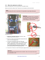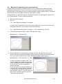
1
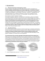
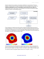
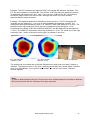
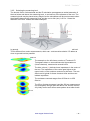
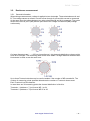
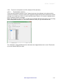
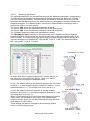
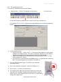
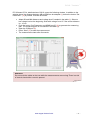
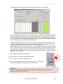
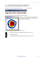
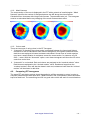
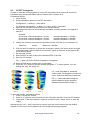
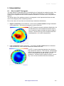
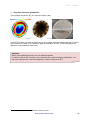
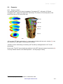
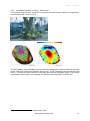
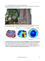
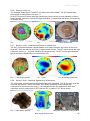
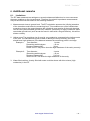
PiCUS Tree Inspection Instruments PiCUS : Treetronic Electrical Impedance Tomograph for trees PC software version Q72.x * February 2010 argus electronic gmbh Joachim-Jungius-Straße 9 18059 Rostock Germany Tel.: +49 (0) 381-4059 324 www.argus-electronic.de PiCUS : Treetronic Table of contents 1. Introduction .................................................................................................................. - 3 1.1. Electrical impedance tomography on trees........................................................... - 3 1.2. Operational theory ............................................................................................... - 3 2. PiCUS : Treetronic technical notes ............................................................................ - 5 2.1. Contents of measuring case................................................................................. - 5 2.2. Conditions for taking measurements .................................................................... - 5 2.3. Electrodes ............................................................................................................ - 6 3. EIT Measurements ...................................................................................................... - 7 3.1. General notes ...................................................................................................... - 7 3.2. Determine the level, number, and positions of measuring points .......................... - 7 3.2.1. General notes............................................................................................... - 7 3.2.2. Number of measuring points ........................................................................ - 7 3.2.3. Installing the nails ......................................................................................... - 9 3.2.4. Placing MP in decayed areas? ..................................................................... - 9 3.2.5. Selecting the measuring level ..................................................................... - 10 3.3. Mount the equipment on the tree ....................................................................... - 11 3.4. Measure the geometry at the measuring level .................................................... - 12 3.5. Resistance measurement .................................................................................. - 13 3.5.1. General information .................................................................................... - 13 3.5.2. Treetronic configuration (for PC software Q72.4 and later) ......................... - 14 3.5.3. EIT measuring process .............................................................................. - 16 3.6. Calculate the Electrical Impedance Tomogram (EIT) ......................................... - 19 4. Software description .................................................................................................. - 20 4.1. Calculation options ............................................................................................. - 20 4.1.1. Smoothness ............................................................................................... - 20 4.1.2. Mesh fineness ............................................................................................ - 21 4.1.3. Colour scale ............................................................................................... - 21 4.2. Comparing EIT tomograms ................................................................................ - 21 4.3. 3-D EIT Tomograms........................................................................................... - 22 5. Interpretation ............................................................................................................. - 23 5.1. How to read EI Tomograms ............................................................................... - 23 5.2. Examples ........................................................................................................... - 26 5.2.1. Decay or cavity? ......................................................................................... - 26 5.2.2. Crack/Bark inclusion or decay – beech tree?.............................................. - 27 5.2.3. Crack/Bark inclusion or decay? Sequoia Giganteum .................................. - 28 5.2.4. Activity of fungus infection .......................................................................... - 29 5.2.5. Decay or cavity (I) ...................................................................................... - 29 5.2.6. Decay or cavity (II) ..................................................................................... - 30 5.2.7. Decay in roots – Kretschmaria Deusta on a beech tree .............................. - 30 5.2.8. Decay in roots – Meripilus Giganteus on a beech tree ................................ - 30 6. Additional remarks ..................................................................................................... - 31 6.1. Limitations.......................................................................................................... - 31 6.2. Possible problems.............................................................................................. - 32 6.2.1. Net generator ............................................................................................. - 32 6.2.2. Bad data..................................................................................................... - 32 7. Safety information and general hints .......................................................................... - 33 8. Technical information................................................................................................. - 34 8.1. Accumulators and charging ................................................................................ - 34 8.1.1. Changing the accumulator.......................................................................... - 34 8.2. Technical specifications ..................................................................................... - 35 9. Abbreviations ............................................................................................................. - 35 10. Contact information ................................................................................................ - 35 - www.argus-electronic.de -2- PiCUS : Treetronic 1. Introduction 1.1. Electrical impedance tomography on trees Electric Impedance Tomography (EIT, also called electrical resistive tomography) is an inspection method originally developed in the field of geophysics. It uses electric voltage and current, supplied by electrodes placed on the surface of the earth or in bore holes, to locate anomalies in resistance due to underground water, etc. EIT methods were first applied to trees in 1998 by two geophysics, Just and Jacobs. The PiCUS : Treetronic Tomograph uses the working principles of EIT to inspect the resistance of wood in trees. Resistance can by influenced by water content, cell structure, ion concentration, and other factors in wood. Why should I use the EIT inspection method? Our original tomography instrument - the PiCUS Sonic Tomograph - gives you information about how the wood in a certain tree transmits sonic waves. It measures the sonic velocity, which is determined by the relation between the modulus of elasticity (MOE) and wood density. Because both MOE and density correlate strongly with the soundness of the wood, sonic velocity is a good indicator of internal problems in trees. Yet sonic tomography (SoT) cannot always answer all questions about the quality of the wood at the tomography level. In some situations the sonic investigation is altered by the internal structure of the wood1. This makes it necessary to consider using an additional inspection method which relies on other aspects. By combining SoT and EIT, which are based on different working principles, we gain two different types of information about wood. Using both sonic and resistance information enables you to make a more thorough analysis of a tree. 1.2. Operational theory The electrical resistance and its reciprocal, electrical conductivity, are physical properties that allow you to make conclusions about the structure of objects. Electrical resistance tomography is used to determine the spatial resistance distribution in a non-destructive manner. Low resistance can indicate increased moisture content, whereas hollowed structures cause increased levels of resistance. However, in order to appraise the health and stability of trees based on resistance, you need to have a lot of experience. The measurements rely on point-like electrodes (nails) placed around the boundary of an object. A current is injected into the object with two of these electrodes. The resulting electric field depends on the resistance distribution and is measured in pairs by the other electrodes in order to obtain a potential difference (voltage). The following figure shows the electric potential for homogeneous conductivity distribution in normal wood (left). In cases where there is an increased anomaly (centre), the potential lines are moved outwards and we observe increased voltage around the periphery. If the anomaly is more conductive than the background (right), the potential lines are attracted and we see lower resistance. “I” – current is applied and measured, “U” – Voltage is measured 1 Please see the PiCUS Sonic Tomograph manual for more information. www.argus-electronic.de -3- PiCUS : Treetronic After all measurements are taken, the resistance distribution is reconstructed. The main problem in using a numerical solution to describe the interior resistance from the measured voltages is the ambiguity, i.e. a variety of models can be used to explain the data. By introducing additional constraints, e.g. demanding a smooth model, we can restrict such ambiguity and yield a unique solution. This procedure is a non-linear reconstruction solved iteratively, as shown in the following scheme: First the geometry is described and the domain is disjointed (parameterised) into pieces of constant resistance. In the course of iterations, the values are subsequently altered and used to simulate a measuring cycle. As soon the simulated values agree with the observed values, the model can be displayed with a coloured distribution. This is done for the two anomalies we saw earlier, conductive (left) and resistive (right). The electrode survey used determines the reliability and resolution. The more accurate and dense our measurements, the better we are able to determine the resistance distribution. It is also necessary to measure the shape of the tree accurately in order to obtain accurate results. The colours in the EI Tomograms represent values in the unit [Ohm * meter]. www.argus-electronic.de -4- PiCUS : Treetronic 2. PiCUS : Treetronic technical notes 2.1. Contents of measuring case This photo shows the Treetronic instrument in the transporting case. We recommend always using the PiCUS : Treetronic together with the PiCUS Sonic Tomography unit. This allows you to power the Treetronic with the PiCUS power supply. If you wish to use the Treetronic in a stand-alone mode, you will need an additional PiCUS power supply, which you can place in the empty square on the left in this case. The measuring case contains the following items # 1 2 3 4 5 6 7 8 Qty 1 4 2 1 1 1 1 1 Item Treetronic instrument Measuring cables (1-6, 7-12, 13-18, 19-24) 2 pieces of 6-in-one extension cables User manual Power supply (optional) AC/DC Converter – Charger with cable (optional) USB cable (optional) Strap (optional) Extension cables The length of the black/red cables may be too short to measure larger trees. Use the extension cables to reach the distant measuring points. Connect the extension cables as shown here: 2.2. Conditions for taking measurements Trees change their moisture content continuously over the course of the year, but experience shows us that the relation between low-impedance areas and high-impedance areas remains approximately constant. This means that areas of relative high conductivity, such as the ring of sapwood and bark, shown in blues in an EIT, are more conductive than the “dryer” heartwood in spring, summer, www.argus-electronic.de -5- PiCUS : Treetronic autumn and winter. The heartwood of the tree is less conductive throughout the year and is therefore shown in reds. However, the absolute values of the resistance calculated can vary. Each tree species has its own typical resistance distribution, and it is important to know the normal resistance distribution of a certain tree species in order to read an EI Tomogram. Temperatures near and below zero degrees (Celsius) can make an electrical impedance tomogram (EIT) more difficult to understand. We recommend not using the EIT unit during or after periods of frost. 2.3. Electrodes In general you can use any type of conductive metal electrodes to take EIT measurements. We recommend electrical galvanized nails, which can be used for taking both sonic and electric impedance measurements. www.argus-electronic.de -6- PiCUS : Treetronic 3. EIT Measurements 3.1. General notes There are several steps involved in taking a PiCUS : Treetronic® measurement: 1. Determine the level, number, and positions of measuring points (section 3.2) 2. Mount equipment on the tree (section 3.3) 3. Measure the geometry at the measuring level (section 3.4) 4. Resistance measurement (section 3.5) 5. Calculate the tomogram (section 3.6) The following sub-sections describe these different procedures. Note: Check that all batteries (PiCUS power supply, PiCUS Calliper, Laptop PC) have sufficient voltage BEFORE you leave your office. 3.2. Determine the level, number, and positions of measuring points 3.2.1. General notes Before starting to work on a tree, you must decide: at which level you wish to measure, where to place the measuring points (MP), and how many points to use. Look for external signs of internal defects, such as fungus growth, cracks, cavities, damaged bark, etc. Use all of your knowledge about trees and diseases and choose the measuring level according to your visual assessment of the tree. You should also examine the tree near ground level, as many types of fungus grow from the root system upwards into the trunk. 3.2.2. Number of measuring points The more MPs used, the better the results will be. The distance between MP should be roughly the same all around the circumference. The number of MP and distance between them determines the level of resolution of the EI Tomogram. The resolution in the centre of the trunk is lower than on the edges. The maximum distance between MP: The minimum distance between MP: ~ 20-25 cm *) ~ 1 cm *) The actual distance between MP can be larger than 25 cm, but resolution around the edges of the trunk is limited. Sapwood cannot be found if distance between the MP is too large. In many cases it is best to use twice as many MP as you would use for SoT measurements. www.argus-electronic.de -7- PiCUS : Treetronic Example: The SoT measurement required 10 MP, the average MP-distance was 20cm. The EIT will require between 10 and 20 MP. The number of MP can easily be doubled by placing an additional nail between two “SoT” nails. If you use only 10 MP for the EIT, the accuracy around the edges of the trunk will be lower, although the centre of the tree will have approximately the same resolution. Example: The sapwood thickness is estimated to be around 5 cm. The EIT tomogram will need MP set at a distance of ~ 4 to 8 cm in order to display the thickness correctly. The tomograms below demonstrate this case: The 10MP EIT used a MP distance of 9-10 cm. The thickness of the high conductive (blue) ring can be measured in the tomogram: ~5 cm. By doubling the number of MP and creating a 20MP-EIT, the MP-distance was decreased to ~4.5 cm. The 20MP-EIT determines a blue ring thickness of ~3 cm. The actual size of the high conductive ring – shown in the photo on the right - is between 2 and 3 cm. EIT using 20 MP Values: ~3 cm EIT using 10 MP Values: ~5 cm Photo of sapwood The largest tree ever tested was a Sequoia Sempervirens which was more than 5 meters in diameter. The bigger the tree is, the more measuring points (MP) are needed. Each Treetronic device has 24 channels. If you need to set more MP, you can link up to three Treetronic devices together. Note: In order to detect/measure the size of outer layers such as bark/sapwood, the distance between MP should coincide with the thickness of the layer expected. www.argus-electronic.de -8- PiCUS : Treetronic 3.2.3. Installing the nails You always need an even number of MP to take EIT measurements. The nails must be touching the wood itself. Make sure that nails are longer than the thickness of the bark so that they penetrate past the outer bark. Nails must not be rusty. Rust can electrically insolate the nail and block the measurements. Tap in the nails for your measuring points along an imaginary straight (horizontal) line. 3.2.4. Placing MP in decayed areas? When taking EIT measurements, you will need to place MP in damaged areas as well. This is different than when taking sonic measurements (SoT). For EIT, you will want to have MP positions which are equidistant. MP should also be placed in damaged areas because the altered properties of the damaged wood can be detected better this way. www.argus-electronic.de -9- PiCUS : Treetronic 3.2.5. Selecting the measuring level The electric field is 3-dimensional and the EI calculation presupposes a vertical extension of the tree below and above the measuring level, to a minimum of the diameter of the tree. The measuring level may be placed at any height, but the calculations will be most accurate when the distance between the measuring level and the root or fork (etc.) is 0.5 to 1 times the diameter of the tree. Please see these examples: In general, measurements near the roots should be at least 20 to 40 cm above ground level. This is different from sonic measurements, which can - and sometime should - be taken as close to ground level as possible. 208 cm The example on the left shows a series of Treetronic EI Tomograms taken on a sound Aesculus hippocastanum (Horse chestnut), measured at several levels. 1) The blue colours (1) indicate lower impedance in the centre of the tree. The impedance of the centre gets higher at the upper levels, so the moisture content may be lower. The wetwood core is typical for horse chestnut trees and does not indicate a problem. The resistance contrast ranges from 20 Ohm*m to 250 Ohm*m. The 25 cm (bottom tomogram) and the 208 cm measurement (top tomogram) infringe upon the above rule, but the result is very likely correct as it shows same pattern as at other levels. 25 cm www.argus-electronic.de - 10 - PiCUS : Treetronic 3.3. Mount the equipment on the tree Mount the equipment on the tree as shown in the photo below. Make sure that the cables of the Treetronic are connected to the correct nails. Note: Incorrect setup will result in invalid data. It is impossible to repair data afterwards. Attention! Sonic sensors should not be connected to the nails when the EIT measurements are performed! The voltage of the Treetronic could damage the sonic sensors! Proceed as follows: 1. Mount the Treetronic instrument to the tree, near measuring point (MP) number 1. 2. Be sure you have removed all sonic sensors from the nails to avoid damaging them. 3. Connect the electrodes to the nails. Electrode number 1 is connected to MP 1, etc. If you have taken a sonic reading before, check that that MP1 of your SoT coincides with MP 1 of the EIT measurement. If you do not need all electrodes of a connector, keep the unused electrodes on the spooling frame. 4. Connect the Treetronic to the PiCUS power supply with the long 7-pin PiCUS Data cable. Attention: Do not connect the electrodes with one another. Also, do not mount more than one electrode to a nail. www.argus-electronic.de - 11 - PiCUS : Treetronic 3.4. Measure the geometry at the measuring level In most cases you will have recorded a PiCUS Sonic Tomogram before taking Electrical Impedance measurements. Thus the first nails are already in place and the geometry has been recorded. If the geometry has not yet been recorded, please read the section “Geometry” in the PiCUS Sonic Tomograph manual or in the Calliper manual. As noted earlier, it is often best simply to double the number of measuring point used for the SoT measurements. To do so, proceed as follows: 1. Start the PiCUS program. 2. Click on File New Electrical Impedance Tomogram to open a new Treetronic file. One of the options allows you to use a file from the sonic tomograph (extension *.pit) in order to import the geometry: File New Electrical Impedance Tomogram Use Tree data from “.pit” file 3. If the geometry does not exist, create a new geometry using Measurement Tree Geometry 4. Electric impedance measurements give better results if many MP are used, so you should use as many points as possible. When using the geometry of an existing sonic file (*.pit), it often makes sense to simply double the number of MP. Click on: Measurement Tree Geometry 2 x MP in order to double the number of MP. This function doubles the number of measuring points by placing a new MP in between all of the “old” MP. The old number MP1 is also the new MP1. A new nail needs to be placed between the “old” MP nails. In many cases the accuracy of the geometry recorded this way will be good enough. However, in some cases you will need to record the geometry correctly. The screen looks like this: www.argus-electronic.de - 12 - PiCUS : Treetronic 3.5. Resistance measurement 3.5.1. General information When taking measurements, voltage is applied to two electrodes. These electrodes are A and B. This voltage causes an electric current to flow through A to B and this current is measured. At the same time the voltage between two other electrodes (M and N) is measured. The points where the current is put in (AB) and the point where the voltage is measured (MN) change continuously. On large diameter trees ( ~ > 350 cm circumference) this electrode distribution scheme might have to be changed. The measuring data will be more stable if a larger distance between M an N electrode is used, as can be seen here:. Up to three Treetronic devices can be used in tandem if the number of MP exceeds 24. The number of measuring points specified determines the number of Treetronic boxes used. Each Treetronic has 24 channels. In case there are 36 measuring points the channel distribution is like this: Treetronic 1 (Address = 71) will cover MP 1 to 24. Treetronic 2 (Address = 72) will cover MP 25 to 36. www.argus-electronic.de - 13 - PiCUS : Treetronic 3.5.2. Treetronic configuration (for PC software Q72.4 and later) 3.5.2.1. Tab Hardware selection There are two firmware versions of the Treetronic devices (the software in the device which controls all functions). The first version was supplied through 2009 and the subsequent version (Version 12) is valid as of 2010. You will need this newer Version 12 in order to operate two or more Treetronic devices in tandem. Before the Treetronic can be used, you will have to indicate the firmware version you are using in the configuration window (1). This must be done for every PC you use with the unit. (1) The “Allocation” map specifies how the electrodes are mapped when two or more Treetronics (e.g. more than 24 MP) are used. www.argus-electronic.de - 14 - PiCUS : Treetronic 3.5.2.2. Measuring parameters The electrode distribution can be specified using the tab “Measuring parameter” (image below). This table shows the standard measurements or settings that occur and allows you to enter your own values as necessary. This table shows the distances between the points of the AB electrodes and the MN electrodes. The distances can vary according to the space between the B and M electrodes. The “Measuring plan” allows you to chose between trees larger than or smaller than 350 cm in circumference. The column “BM” shows the set distance between B and M. The column “AB” shows the distance between the A and B electrodes. The column “MN” shows the distance between the M and N electrodes. The “V-Level” shows the voltage level set between A and B. The “Max BM dist used” selection on the right allows you to chose the maximum distance between B and M. This maximum can only be half the value of the total number of MP, 12 at most for 24 MP. The image on the right shows how the distance between MP-B and MP-M is counted: the distance in-between MP 2 (B) and MP 13 (M) is 11 MP. The distance between MP 1 (A) and MP 14 (N) is 11 as well. B-M distance = 11 [MP] (1) (2) In screen shot of the “measuring parameter” window (above) you see values for a tree larger than 300 cm. There is no distinct circumference to switch to the adaptable setup. In row 1 the default values for the distances between the electrodes B and M ( = 1) determines the distance between A and B (= 1) and between M and N (= 1). The voltage level here is set at 4 (1). In row 8 the distance between B and M is 8, and the distance between A and B is thus 1, the distance between M and N is 3, and the voltage level is set at 5 (2). When a new measuring file is opened the table displays the default values, which are accurate in most cases. If the measurement quality is not very good, you can alter these values using the dropdown buttons in each column. These settings can also be changed in the measuring window shown in the following sections. B-M distance = 1 [MP] B-M distance = 8 [MP] M-N distance = 3 [MP] www.argus-electronic.de - 15 - PiCUS : Treetronic 3.5.3. EIT measuring process To run the EIT measurement proceed as follows: 1. Measurement Electric Tomography measurement or click the icon to open the measuring window. Enter a name for the new Treetronic file. PC Software Q71.9 to Q72.3, distributed through 2009 opens the following measuring window 5) 1) 2) 3) 6) 4 4) 2. In this window click on Voltage level (AB) “Same to all” (1). This causes the program to use the same voltage for all measurements. (The option “Individual” allows you to use different voltages depending on the distance between the points AB and MN.) Select a low voltage level at the beginning. Start with voltage “level 4” (2) if the sensor distance is > 10 cm. Push the button “Set Parameter and ABMN config” (3) to generate the measuring plan. The measuring plan is now shown in the table (4). 3. Turn the (PiCUS) power supply. The LED on the Treetronic should flash twice. 4. Click on the tabulator “Automatic”. Open the COM port (5). 5. Press “Start” (6) to start the measurement. 6. The measurement starts after 3 seconds. Most of the time both “Amp-AB” and “Volt-MN” indicators should be shown in green or yellow colours. If they appear more in red colours, you will need to change the voltage level. www.argus-electronic.de - 16 - PiCUS : Treetronic PC Software Q72.4, distributed as of 2010, opens the following window. In addition to the window above the distance between AB and BM can be adapted (1) before the button “Set Parameter..” (2) is pushed. Proceed as follows: Adapt AB and MN distances and voltage level if needed in the table (1). Select a low voltage level at the beginning. Start with voltage “level 4” if the sensor distance is > 10 cm. Push the button “Set Parameter and ABMN config” (2) to generate the measuring plan. The measuring plan is now shown in the table (3). Open the COM port (4). Press “Start” (5) to start the measurement. The measurement starts after 6 seconds. 4) 1) 2) 5) 3) Attention! Do not touch the cables or the tree while the measurements are running! There is a risk of electric shock while current is present. www.argus-electronic.de - 17 - PiCUS : Treetronic Pay attention to the following hints when the measurement is in progress. 4 4) 1 5 4) 4) 2 4) 3 4) If the current indicator “Amp-AB” (2) and volt indicator “Volt-MN” (3) appear red often, the current/ voltage can be checked in the table. The AB-current is shown in the column “I” (1) in [Ampere] and should range approximately from 0.001 to 0.013 Ampere. If the ABcurrent is smaller, try using a higher voltage level (4). If the current indicator “Amp-AB” (2) is on the upper level, try using a lower voltage level. The MN-Voltage is shown in column “U” (5) in [Volt] and should vary from 0.005 to 2.4 Volt. If the voltage measured is below 0.005 Volt try to use a higher voltage level. If the voltage is greater than 2.3 Volt try to use a smaller voltage level. High voltage/current can cause an overrun on the “Analogue to Digital” converter (ADU) in the Treetronic. In this case the current and voltage measured do not change any more. Wrong values (0 Ampere and 2.5 Volt) are shown. In this case the Treetronic needs be turned off. You will need to before continuing with the measurements, roughly 20 minutes, while the device recovers. 7. Wait until the measurements are done. 8. Press “OK” to close the measurement window. 9. File Save to save the measurement. 10. Run the calculation to see the results. Click “File” “Save” again to save the tomogram calculated in the measuring file. Attention! Do not touch the tree or any of the wires while the measurements are being taken. Voltages can reach up to 100 Volt. www.argus-electronic.de - 18 - PiCUS : Treetronic 3.6. Calculate the Electrical Impedance Tomogram (EIT) In order to calculate the EIT go to the main menu and click on Calculation Electrical Impedance Tomogram or click the icon It can take between 5 to 60 seconds for the results to appear. Click “File save” to save the tomogram shown in the file. When re-loading the file, the tomogram is shown without re-calculating. The EI Tomogramms are scaled with rainbow colours: Blues indicate areas of low impedance (high water content, etc.) Increasing impedance Reds indicate areas of high impedance (lower water content, etc.) www.argus-electronic.de - 19 - PiCUS : Treetronic 4. Software description 4.1. Calculation options To access the calculation options click on Configuration Settings Calculation “Smooth tree shape”: Set this check to draw the edge of the cross-section with a round curve rather than a polygon. 4.1.1. Smoothness The smoothness level determines how many details are shown in the EIT. Low smoothness values (1, 3, 10) will display more details than larger values (100), but they may also suffer more from measuring errors. Smoothness level 20 (the default) is a well-balanced value. The data quality is high when the EIT calculated with low smoothness values (1, 3, 10) is similar to EIT calculated using larger values (20, 30). The tomogram must be re-calculated before any changing of the smoothness value takes effect. The example shows the data of a Sequoia Giganteum, circumference at the measuring level is 810cm. The sonic data (SoT) raised the suspicion that there could be significant cracks. The EIT calculated with smoothing 1 (meaning very sharp interpretation of data) shows the likely positions of the cracks most clearly. These positions coincide with those calculated in the SoT. Smoothness 1 Smoothness 3 Smoothness 20 www.argus-electronic.de - 20 - PiCUS : Treetronic 4.1.2. Mesh fineness The cross-section of the tree is displayed in the EIT with a network of small triangles. “Mesh fineness” specifies the number of triangles between two MP along the circumference. Calculation time increases with rising mesh fineness. The standard value is 4. The tomogram must be re-calculated before any changing of the mesh fineness takes effect. Mesh 2 Mesh 4 Mesh 8 4.1.3. Colour scale There are two ways of using colour in the EI Tomogram: 1. “Automatic” is checked: the colours scale is stretched between the lowest and highest resistance of the file calculated: Dark reds are assigned to the highest resistance levels, dark blues are assigned to lowest resistance calculated. Sound trees of certain species may have a small variation in resistance across the cross-section, for instance only 30 Ohm * meter. With the “Automatic” option, even these tomograms will show the full colour scale from red to blue. 2. “Automatic” is un-checked: Dark red colours are assigned to the “maximal resistor” value. Dark blues are assigned to the “minimal resistor” value. Resistance larger than the “maximal resistor” value will also be drawn in dark red; resistance lower than the “minimal resistor” will be shown in dark blue. 4.2. Comparing EIT tomograms The same EIT calculation options should be applied to all files recorded on a tree in order to compare measurements with each other. “Mesh fineness” and “Smoothness” factors should be kept at a fixed level. The smoothing level 20 is a good value which will work for most situations. www.argus-electronic.de - 21 - PiCUS : Treetronic 4.3. 3-D EIT Tomograms In order to calculate 3-D tomograms of a tree, the measurements at each level need to be calculated using similar calculation options. Please refer to section 4.14. Proceed as follows: 1. Close all files. 2. Select calculation options for the EIT calculation Configuration Settings Calculation For instance Smoothness = 4, Mesh = 6, Colour scale = “Automatic” 3. Open all files recorded on the tree and run the calculations. 4. Write down the minimum and maximum resistance recorded, shown in the legend of each EIT. Example: 20 cm scan: minimal resistance = 23 Ωm; 60 cm scan: minimal resistance = 46 Ωm; 60 cm scan: minimal resistance = 39 Ωm; maximal resistance = 318 Ωm maximal resistance = 290 Ωm maximal resistance = 450 Ωm 5. Identify the minimum and maximum resistance levels of all files. In our example it is: 23 Ωm; Minimum: Maximum = 450 Ωm 6. Click on each file opened, un-check the “Automatic” option in the colour scale, and type in these boundary values. When the “Automatic” option is selected, all tomograms will use a different scale. 7. Re-calculate all files. 8. Save each file in order to store the calculated EITs in the files. 9. Start the 3-D window File New 3-D view of Electric Impedance Tomograms 10. Select all files where images been re-calculated. 11. Press the “3-D” button to see the twisting tomogram. “F1” shows options. You can change the view, the angle, etc. EIT 1 was calculated in “Autoscale” colour mode. All tomograms use the full colour scale from dark blue to dark red. (1) . EIT 1 (1) . EIT 2 EIT 2 + 3 were calculated using the same resistance range: variations between levels become visible (1). EIT 3 To save the images, proceed as follows. 1. Push “s” to stop the motion. 2. Push “p” to copy the current screen into the 3-D project window. Close the 3-D window. 3. “Right click” in the right window to open an on-screen menu. Select “save” to save the image. Alternatively the “alt” + “print” keys can be used to copy the current screen into the window clipboard. From here it can be pasted into other image-processing programs. www.argus-electronic.de - 22 - PiCUS : Treetronic 5. Interpretation 5.1. How to read EI Tomograms The main aspect of interpreting EITs is the distribution of high and low conductive areas. You are looking to see where high resistance is and where low resistance is. This information needs to be compared with the normal resistance distribution in sound trees of this particular species. The actual value of the resistance given in a tomogram is less important and less accurate, due to the ambiguity of the measuring method. Due to the nature of trees there are several major resistance distributions: 1. Higher conductivity (low resistance – blue colours) on the outside and high resistance (low conductivity – red colours) towards the inside of the tree. This EIT shows the normal resistance distribution of a sound beech tree. The heartwood of beech trees is less conductive (higher resistance) than the edge of the tree. The blue the ring on the outside shows the bark/sapwood (1) for water transportation. (2) (1) 2. Low conductivity (higher resistance – red colours) on the outside and low resistance (high conductivity – blue colours) towards the inside of the tree. The EIT of a sound sequoia giganteum tree shows a high conductive centre (3 - blue colours). The bark/sapwood is less conductive (4- red colours). The absolute values of the sapwood indicate that the wood is conductive – because of the moisture content, it is not dry – but it is less conductive than the heartwood. (3) (4) www.argus-electronic.de - 23 - PiCUS : Treetronic 3. Ring-like resistance distribution This example shows the EIT of a Quercus robur2 (oak). 1) EIT SoT In the EIT the blue ring (high conductivity) on the outside represents bark/sapwood. The blue high conductive centre (1) is caused by high concentration of ions. These tomograms are typical for sound quercus robur trees. Attention: Other normal distributions can occur in different species. In order to read an EIT correctly, you must know the normal resistance distribution. You will need experience for each tree species in order to interpret an EIT. 2 Recorded by argus electronic, Rostock, Germany 2009. www.argus-electronic.de - 24 - PiCUS : Treetronic There are some general rules that can be used to evaluate EIT and Sonic Tomogramms (SoT) in combination: Case 1 – High resistance inside – high conductivity outside The table helps evaluate the centre of the tree SoT Sonic velocity [m/s] High (brown) EIT Resistance [Ω*m] High (red) Conclusion High (brown) Low (blue) Still safe, but early decay Low (blue/violet) High (red) Cavity / dead decay Low (blue/violet) Low (blue) Active decay Healthy Case 2 – Low resistance inside – low conductivity outside The table helps to evaluate the centre of the tree SoT Sonic velocity [m/s] High (brown) EIT Resistance [Ω*m] Low (blue) Conclusion High (brown) High (red) Low (blue/violet) Low (blue) Dead dry solid wood inside (no examples yet found) Active decay Low (blue/violet) High (red) Cavity / dead decay Healthy There are exceptions to these guidelines, depending on tree species, type of fungus, etc. www.argus-electronic.de - 25 - PiCUS : Treetronic 5.2. Examples 5.2.1. Decay or cavity? The example shows a 3-D electric Impedance Tomogram (EIT - left) and a 3-D Sonic Tomogram (SoT - right) of an apple tree3 with decay. The source of the decay was an old branch that was cut off many years ago. 1) 2) 165 cm 140 cm 110 cm 85 cm 3) 30 cm EIT (all slices drawn with same scale) SoT 165 cm scan: EIT high conductivity ((1) - blue area) coincides with low sonic velocity (2): very wet material is in this region, most likely active decay. 140-85 cm scans: decreasing conductivity (EIT less blue), damaged area in SoT is also decreasing. 30 cm scan: The SoT shows hardly any defects, but the EIT shows increased conductivity (3). This may indicate another root-related problem – an early stage of decay. 3 Recorded by argus electronic, Aubonne, Switzerland, 2008. www.argus-electronic.de - 26 - PiCUS : Treetronic 5.2.2. Crack/Bark inclusion or decay – beech tree? The example shows an SoT and an EIT of a beech with three trunks4. Bodies of fungus were found between MP 1 and 12 (SoT). 2) 1) 1) 1) SoT EIT The SoT shows a large damaged area; but there is probably bark inclusion between the three trunks. This bark inclusion will interfere with the SoT. The EIT shows the likely positions of the bark (1). The active fungus infection is very likely the relatively small blue area (2). By using a combination of both types of tomograms, the decision was made NOT to fell the tree. 4 Recorded by Frits Gielissen, The Netherlands, 2008. www.argus-electronic.de - 27 - PiCUS : Treetronic 5.2.3. Crack/Bark inclusion or decay? Sequoia Giganteum This Sequoia tree is in the municipal zoo of Rostock, Germany. It was planted in 1883 and is the oldest living organism in the entire zoo. (1) MP4 MP5 The SoT showed a large area through which the sonic waves could not travel. But the tree also showed indications of cracks or/and bark inclusions at many locations (1). (2) (2) SoT (3) (2) (3) (2) (3) (4) EIT EIT of a sound (but very small) Sequoia tree The crack detection function of the SoT indicated a high likelihood of cracks. Thus, the wood in between those cracks (2) was invisible to the sonic investigation. The EIT of a sound sequoia (on the right) shows that the heartwood is usually highly conductive (blue colour) for these trees. Using this information we were able to analyse the EIT of the large sequoia (in the middle). We were able to conclude that the slow-velocity areas in between the possible cracks in the SoT (2) very likely consisted of intact wood, because the conductivity seemed to be normal (3). The high resistance area (4) appeared to be a cavity. www.argus-electronic.de - 28 - PiCUS : Treetronic 5.2.4. Activity of fungus infection The example shows the SoT and EIT of a linden tree (tilia cordata) with fungus damage5. Bodies of fungus were observed near MP 4 to 8. 3) 3) 3) 2) 1) 1) 1) SoT EIT photo of the linden tree This example shows how different stages of decay are displayed. Old dead decay is found around MP 5-6-7-8: Low sonic velocity AND high resistance (1) Active decay is shown by high conductivity (2) in the EIT and moderate sonic velocity; compared with the advanced decay area. Early stages of decay can be found above the yellow line (3). Sonic velocity is already decreased; the wood is higher conductive (higher moisture content), but no defect is visible. 5.2.5. Decay or cavity (I) The example shows the SoT and EIT of a linden tree (tilia cordata). The SoT shows slowly decreasing velocity from MP 7/8/9 towards the centre (4), represented by light brown colours. In the EIT this area is shown with very high conductivity: a clear indication of an active fungus growth. Low sonic velocity and high resistance (5) show where the cavity is. 5) 4) 4) 5) 5) 4) 4) 4) SoT 5 EIT photo of the linden tree Recorded by argus electronic, Rostock, Germany, 2009. www.argus-electronic.de - 29 - PiCUS : Treetronic 5.2.6. Decay or cavity (II) The example shows the SoT and EIT of a linden tree (tilia cordata). The SoT shows large green areas in many parts of the tree (1). In the EIT this area is shown with high conductivity (blue colours): a clear indication of active fungus growth. Low sonic velocity and high resistance (2) show dead old decay: the beginning of a future cavity. 1) 1) 2) 1) 1) 1) SoT 2) 2) 1) EIT 1) Photo of the trunk 5.2.7. Decay in roots – Kretschmaria Deusta on a beech tree The SoT of this beech shows a typical pattern for a fungus infection: the centre of the trunk does NOT have the darkest colours e.g. highest sonic velocity. The EIT clearly shows the high conductive centre (1) – a typical indication for fungus activity. The EIT on the right shows the typical resistance distribution of a sound beech tree. 1) SoT – 5 cm above ground EIT – 5 cm EIT of healthy beech tree 5.2.8. Decay in roots – Meripilus Giganteus on a beech tree The root system of the beech was infected by Meripilus Giganteus. The 20 cm sonic scan did not show any defects. The EITs at 20cm and 120cm measuring levels indicate high conductivity in the centre of the trunk (1). Sound beech trees are supposed to have less conductive centres (red colours in EIT) than the EIT in section 5.2.7 above shows. 1) 1) 1) SoT – 20cm above ground EIT www.argus-electronic.de Meripilus Giganteus fruiting bodies - 30 - PiCUS : Treetronic 6. Additional remarks 6.1. Limitations The EIT data measured are ambiguous; several resistance distributions in a tree can cause the same readings on the circumference. Therefore, the electric impedance measurements may not show the correct results in the following situations: 1. Measurements close to ground level. The EIT calculation assumes the (infinite) extension of the tree above and below the measuring level. This condition can not be fulfilled when measuring close to the ground because the cylindrical cross-section of the trunk develops into the root system beneath ground level. However, particularly in highly conductive wood near/under ground level (such as can be found in trees with a fungus infection), this will be shown correctly. 2. Hollow trees. The remaining ring of wood is very conductive compared to the hollow centre of the tree. The calculation may not be able to identify the cavity correctly (the cavity should have high resistance) if the distance between the measuring points is too large. Example1: Tree diameter: 1 meter Remaining wall thickness: ~10 cm Distance between MP: 30 cm Result: an EIT may fail to show the high resistance of the cavity correctly. Example 2: Tree diameter: 1 meter Remaining wall thickness: ~10 cm Distance between MP: 5-10 cm Result: the EIT will show the high resistance of the cavity. 3. Water-filled cavities. A cavity filled with water could be shown with blue colours (high conductive) in the EIT. www.argus-electronic.de - 31 - PiCUS : Treetronic 6.2. Possible problems 6.2.1. Net generator The net generator calculates the net of triangles. In rare cases the calculation of the net can fail. This is due to misplacement of sensors. The distance between MPx and MPy is too small and the distance between MPx and the centre (of the tree) is very different to the distance between MPy and the centre. Left: Net generator works well. The distance between the MP is small and the adjacent MP have approximately the same distance to the centre of the tree. Right: Net generator may fail. The distance between the MP is small and the adjacent MP have very different distances to the centre of the tree. The result is a tomogram like this: The large triangles in the centre indicate a problem in one part of the reconstruction software. In some case the problem can be solved if the net fineness is set to 6, 7 or 8. In general it is better to reposition the critical measuring points, in this case 12 and 13. 6.2.2. Bad data On large diameter trees with big cavities or other large defects, the data quality can drop to a level where the tomogram does not give reliable results. One indication for bad data quality is a (red) curve as shown in this example. In this case, you should try to enlarge the voltage level and repeat the measurements. www.argus-electronic.de - 32 - PiCUS : Treetronic 7. Safety information and general hints Do not touch nails, electrodes or the tree during EI measurements! Voltages of up to 100 Volt are possible! Before taking measurements with the Treetronic, remove all sonic sensors the nails! The voltage of the Treetronic can destroy the sonic sensors. from Do not connect the electrodes with one another. Do not mount more than one electrode to each nail. www.argus-electronic.de - 33 - PiCUS : Treetronic 8. Technical information 8.1. Accumulators and charging Note: Do not store accumulator batteries when they are completely empty. If they are totally discharged, the end of the charging process may not be detected correctly and will be terminated after only 15 minutes. Disconnect the charger, wait for 10 seconds, and the reconnect the charger to restart the charging process. The charging time is now 4-6 hours. To charge accumulators proceed as follows: 1. Connect the AC/DC converter supplied to a power socket. Connect the DC plug to the PiCUS charging socket. 2. The charging LED displays a green light when charging. Accumulators can also be charged while taking measurements. 3. The accumulators are fully loaded when the charge LED is off. Depending on the accumulator status, this can take up to 6 hours. Do not forget to charge your PC/PocketPC before going out to take measurements. Warning: Do NOT operate the PiCUS unit without the batteries connected. The charger MUST not be connected to the PiCUS power supply if the batteries are not connected. 8.1.1. Changing the accumulator If the accumulator battery pack needs to be replaced, please proceed as follows: 1. 2. 3. 4. Turn off the PiCUS unit and disconnect all devices and cables from the power supply. Remove the soft cover. Disconnect the cable from the old accumulator. Connect the new accumulator. www.argus-electronic.de - 34 - PiCUS : Treetronic 8.2. Technical specifications The PiCUS Power supply can be used for the Treetronic as well. Charging time: Charging unit at 100 – 240 V~ (AC), 50 Hz NiMH, 3800 mAh As the accumulators get older the number of charging/discharging procedures reduces the capacity. max. 4 hours, (no overloading due to automatic turn-off) Power consumption of: Treetronic: power supply: approx. 190 mA approx. 150 mA Time of operation at 20°C / 0°C: ~ 8 h / ~ 3.5 h Power supply: Type of Accumulator: Accu power: Note: Technical specifications are subject to change without notice. 9. Abbreviations d EIT I MOE MP SoT U Ωm 10. diameter (of the tree) Electric Impedance Tomography or Tomogram Electric current Modulus of Elasticity Measuring Point Sonic Tomography or Sonic Tomogram Voltage Physical unit the EIT is showing: Ohm * meter Contact information The PiCUS : Treetronic was developed by argus electronic gmbh. argus electronic gmbh Joachim - Jungius - Str. 9 18059 Rostock Germany Tel.: +49 - (0) - 381 - 40 59 324 Fax: +49 - (0) - 381 - 40 59 322 www.argus-electronic.de [email protected] Author of this manual: Lothar Göcke; email: [email protected] Date : 04 February 2010 www.argus-electronic.de - 35 -