Download fulltext01 - DiVA Portal

Controller design for an unmanned
surface vessel
Design of a heading autopilot and way-point navigation system for
an underactuated USV.
Geir Beinset
Jarle Saga Blomhoff
Master of Science in Engineering Cybernetics
Submission date: June 2007
Supervisor:
Amund Skavhaug, ITK
Co-supervisor:
Tristan Perez, CeSOS
Norwegian University of Science and Technology
Department of Engineering Cybernetics
Problem Description
1. Obtain a vessel model for control system design based on system identification. The data for the
identification will be obtained from experiments performed on the full scale vessel. Compare the
response of the model to that of the real vessel.
2. Perform design of a heading autopilot in Simulink using the vessel model obtained by system
identification.
3. Design a guidance system that can follow a route consisting of multiple way-points.
4. Implement the heading autopilot and the way-point navigation system on the full scale vessel.
5.Present your findings and results in the report.
Assignment given: 10. January 2007
Supervisor: Amund Skavhaug, ITK
Design of a heading autopilot for a small unmanned surface
vehicle
Jarle Saga Blomhoff and Geir Beinset
Department of Engineering Cybernetics
Norwegian University of Science and Technology—NTNU
June 7, 2007
Abstract
This report is written as a part of a development programme performed by Maritime
Robotics AS. The goal of the programme is to develop an Unmanned Surface Vehicle
(USV) to be used as support for oil search vessels and other offshore activities. Our contribution to this development has been to create an environment for rapid development
and implementation of new controllers for the USV. A way-point navigation system
and a heading autopilot have been designed and implemented using this environment.
The Rapid Control Prototyping (RCP) environment consists of different phases. In the
first step experiments are designed and performed to capture the dynamics of the vessel.
Data from these manouvers are then used during the system identification phase. This
phase creates a mathematical model of the vessel to be used as the “real vessel” during
simulations. Controller design is then performed in Simulink using the identified model
as the plant. When the controller design has reached a satisfactory level, the implementation phase begins. During implementation, the vessel model in Simulink is replaced by
blocks to communicate with the actuators and sensors of the USV. Real-time constraints
are put on the system to be used during implementation.
The results of our Master thesis is a successfully developed and implemented waypoint navigation system and a heading autopilot for the USV. These controllers in
addition to the RCP environment we have created, provides Maritime Robotics with a
solid base for further development of their project. The RCP environment and tuning
of the controllers still needs improvements. But we have even before the Master thesis is
delivered, received indications that Maritime Robotics will use our design during further
work and implement it on other vessels.
Preface
This report is written as a part of the master thesis during the 10th semester at the
Norwegian University of Science and Technology, department of Engineering Cybernetics. This master thesis is a continuation of our project work in the 9th semester. The
work was proposed by Maritime Robotics AS as a support to their development of an
unmanned surface vehicle. It has been a a challenging and interesting project, where
we have gained valuable insight into system identification and project work. We have
been two students working on this task, and the cooperation has worked surprisingly
well. Both fruitful discussions and constructive critics have resulted in the report you
now hold in your hands.
We would also like to thank both Tristan Perez at the Centre for Ships and Ocean
Structures at NTNU and Amund Skavhaug at the department of Engineeing Cybernetics
for valuable professional guidance and constructive suggestions. Moreover we would like
to thank Maritime Robotics AS for allowing us to work on their project and trusting us
with their valuable vessel and equipment.
i
Contents
I
Background
4
1 Vessel and Equipment Configuration
1.1
The Vessel - Kaasbøll 19 . . . . . . . . . . . . . . . . . . . . . . . . . . . .
5
1.2
The Outboard Engine - Evinrude 50 Etec . . . . . . . . . . . . . . . . . .
6
1.3
Measurement Equipment . . . . . . . . . . . . . . . . . . . . . . . . . . . .
7
1.3.1
DGPS Compass - Seatex Seapath 20 . . . . . . . . . . . . . . . . .
7
1.3.2
Simrad RPU80 Rudder pump and LF3000 Rudder Sensor . . . . .
9
Equipment mounting and calculation of CG . . . . . . . . . . . . . . . . .
9
1.4
2 Rapid Control Prototyping
II
5
14
2.1
Simulator . . . . . . . . . . . . . . . . . . . . . . . . . . . . . . . . . . . . 15
2.2
Real-time constraints . . . . . . . . . . . . . . . . . . . . . . . . . . . . . . 15
Modelling
18
3 Experiments
19
3.1
Input design for open loop experiments
3.2
Binary Rudder Manoeuvre . . . . . . . . . . . . . . . . . . . . . . . . . . . 21
3.2.1
Pseudo Random Binary Signal properties . . . . . . . . . . . . . . 21
4 System Identification
4.1
4.2
. . . . . . . . . . . . . . . . . . . 19
26
Rudder Pump System Identification . . . . . . . . . . . . . . . . . . . . . 28
4.1.1
20 knots model . . . . . . . . . . . . . . . . . . . . . . . . . . . . . 30
4.1.2
5 and 12 knots models . . . . . . . . . . . . . . . . . . . . . . . . . 31
Vessel System Identification . . . . . . . . . . . . . . . . . . . . . . . . . . 34
ii
4.2.1
Data pre-treatment . . . . . . . . . . . . . . . . . . . . . . . . . . . 34
4.2.2
5 knots model identification . . . . . . . . . . . . . . . . . . . . . . 39
4.2.3
Best model at 5 knots . . . . . . . . . . . . . . . . . . . . . . . . . 40
4.2.4
12 knots model identification . . . . . . . . . . . . . . . . . . . . . 42
4.2.5
Best model at 12 knots . . . . . . . . . . . . . . . . . . . . . . . . 44
4.2.6
20 knots model identification . . . . . . . . . . . . . . . . . . . . . 47
4.2.7
Best model at 20 knots . . . . . . . . . . . . . . . . . . . . . . . . 48
5 Discussion
51
6 Conclusion
54
III
56
Control Design
7 Theory
7.1
57
PID control . . . . . . . . . . . . . . . . . . . . . . . . . . . . . . . . . . . 58
7.1.1
Proportional Control . . . . . . . . . . . . . . . . . . . . . . . . . . 59
7.1.2
Integral Control . . . . . . . . . . . . . . . . . . . . . . . . . . . . 59
7.1.3
Derivative Control . . . . . . . . . . . . . . . . . . . . . . . . . . . 60
7.1.4
Set Point Weighting . . . . . . . . . . . . . . . . . . . . . . . . . . 62
7.1.5
Integrator Windup . . . . . . . . . . . . . . . . . . . . . . . . . . . 63
7.1.6
Bumpless transfer . . . . . . . . . . . . . . . . . . . . . . . . . . . 64
7.1.7
Digital Implementation . . . . . . . . . . . . . . . . . . . . . . . . 66
7.1.8
Manual parameter tuning and the Ziegler-Nichols methods . . . . 68
7.2
Reference model . . . . . . . . . . . . . . . . . . . . . . . . . . . . . . . . 72
7.3
Gain Scheduling . . . . . . . . . . . . . . . . . . . . . . . . . . . . . . . . 73
7.4
Way-Point Navigation System . . . . . . . . . . . . . . . . . . . . . . . . . 73
8 Design in Simulink
75
8.1
Reference model . . . . . . . . . . . . . . . . . . . . . . . . . . . . . . . . 75
8.2
Heading Controller . . . . . . . . . . . . . . . . . . . . . . . . . . . . . . . 78
8.2.1
Discontinuous heading measurement (0◦ -359◦ )
8.2.2
Ziegler-Nichols experiments . . . . . . . . . . . . . . . . . . . . . . 86
8.2.3
Limited Derivative Action . . . . . . . . . . . . . . . . . . . . . . . 91
iii
. . . . . . . . . . . 81
8.2.4
Root Locus tuning of the parameters . . . . . . . . . . . . . . . . . 91
8.2.5
Proportional set-point weighting . . . . . . . . . . . . . . . . . . . 97
8.2.6
Integrator anti-windup . . . . . . . . . . . . . . . . . . . . . . . . . 98
8.2.7
5 and 12 knots controller . . . . . . . . . . . . . . . . . . . . . . . 101
8.2.8
Manual mode and Bumpless transfer . . . . . . . . . . . . . . . . . 104
8.2.9
Disturbances . . . . . . . . . . . . . . . . . . . . . . . . . . . . . . 104
8.2.10 Stability and sensitivity analysis . . . . . . . . . . . . . . . . . . . 106
8.3
8.4
Gain Scheduler . . . . . . . . . . . . . . . . . . . . . . . . . . . . . . . . . 109
8.3.1
Interface between Stateflow and Simulink . . . . . . . . . . . . . . 110
8.3.2
States . . . . . . . . . . . . . . . . . . . . . . . . . . . . . . . . . . 111
8.3.3
State actions and variables . . . . . . . . . . . . . . . . . . . . . . 113
8.3.4
State transitions . . . . . . . . . . . . . . . . . . . . . . . . . . . . 116
8.3.5
Triggering the chart . . . . . . . . . . . . . . . . . . . . . . . . . . 117
Way-Point Navigation . . . . . . . . . . . . . . . . . . . . . . . . . . . . . 117
9 Implementation
9.1
119
Communication, hardware and Real-Time Constraints . . . . . . . . . . . 119
9.1.1
Sampling times . . . . . . . . . . . . . . . . . . . . . . . . . . . . . 119
9.1.2
Read NMEA messages . . . . . . . . . . . . . . . . . . . . . . . . . 120
9.1.3
Read rudder angle . . . . . . . . . . . . . . . . . . . . . . . . . . . 124
9.1.4
Voltage Out to Rudder Pump . . . . . . . . . . . . . . . . . . . . . 125
9.2
Rudder angle controller . . . . . . . . . . . . . . . . . . . . . . . . . . . . 126
9.3
Navigation System and Heading Controller . . . . . . . . . . . . . . . . . 129
9.4
9.3.1
Heading Autopilot without Gain Scheduling . . . . . . . . . . . . . 129
9.3.2
Heading Controller with Gain Scheduling . . . . . . . . . . . . . . 129
9.3.3
Way-point Navigation System . . . . . . . . . . . . . . . . . . . . . 131
Graphical User Interface (GUI) . . . . . . . . . . . . . . . . . . . . . . . . 134
10 Discussion
136
11 Conclusion
140
Appendices
142
iv
A MATLAB Code
142
A.1 PRBS spectrum.m . . . . . . . . . . . . . . . . . . . . . . . . . . . . . . . 142
A.2 import data.m . . . . . . . . . . . . . . . . . . . . . . . . . . . . . . . . . 142
A.3 parseLabViewLog.m . . . . . . . . . . . . . . . . . . . . . . . . . . . . . . 142
A.4 setparam(values) . . . . . . . . . . . . . . . . . . . . . . . . . . . . . . . . 143
A.5 ZNstepResponse.m . . . . . . . . . . . . . . . . . . . . . . . . . . . . . . . 143
A.6 ZNultimateSensitivity.m . . . . . . . . . . . . . . . . . . . . . . . . . . . . 144
A.7 VariableTuning.m . . . . . . . . . . . . . . . . . . . . . . . . . . . . . . . . 144
A.8 USVsimulationGui.m . . . . . . . . . . . . . . . . . . . . . . . . . . . . . . 145
A.9 run.m . . . . . . . . . . . . . . . . . . . . . . . . . . . . . . . . . . . . . . 145
A.10 Serial configuration . . . . . . . . . . . . . . . . . . . . . . . . . . . . . . . 145
A.11 NMEAserread sfun.m . . . . . . . . . . . . . . . . . . . . . . . . . . . . . 147
A.12 serread sfun.m . . . . . . . . . . . . . . . . . . . . . . . . . . . . . . . . . 148
A.13 serwrite sfun.m . . . . . . . . . . . . . . . . . . . . . . . . . . . . . . . . . 148
B Measurement pre-treatment plot
B.1 5 knots
149
. . . . . . . . . . . . . . . . . . . . . . . . . . . . . . . . . . . . . 149
B.2 12 knots . . . . . . . . . . . . . . . . . . . . . . . . . . . . . . . . . . . . . 151
B.3 20 knots . . . . . . . . . . . . . . . . . . . . . . . . . . . . . . . . . . . . . 153
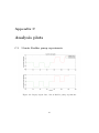
C Analysis plots
155
C.1 5 knots Rudder pump experiments . . . . . . . . . . . . . . . . . . . . . . 155
C.2 12 knots Rudder pump experiments . . . . . . . . . . . . . . . . . . . . . 159
C.3 20 knots Rudder pump experiments . . . . . . . . . . . . . . . . . . . . . 163
C.4 Ziegler-Nichols step response analysis . . . . . . . . . . . . . . . . . . . . . 167
C.5 Ziegler-Nichols ultimate-sensitivity analysis . . . . . . . . . . . . . . . . . 170
C.6 Ziegler-Nichols step-response vs. ultimate-sensitivity analysis . . . . . . . 172
D Table of Contents - CD
174
v
List of Figures
1
Work flow from problem specification to implementation . . . . . . . . . .
3
1.1
Kaasbøll 19 feet centre console boat, (Kaasbøll Boats AS) . . . . . . . . .
5
1.2
Outboard engine Evinrude 50 E-tec, (Kaasbøll Boats AS) . . . . . . . . .
7
1.3
Measurment set-up . . . . . . . . . . . . . . . . . . . . . . . . . . . . . . .
8
1.4
Seapath 20 DGPS sensor, (www.km.kongsberg.com) . . . . . . . . . . . .
9
1.5
Hydraulic steering system, (www.simradyachting.com) . . . . . . . . . . . 10
1.6
CAD drawing of the boat with CG, sideview . . . . . . . . . . . . . . . . 11
1.7
CAD drawing of the boat with CG, overview . . . . . . . . . . . . . . . . 12
2.1
Traditional vs rapid prototyping design of a controller . . . . . . . . . . . 14
2.2
The flow of a rapid prototyping process . . . . . . . . . . . . . . . . . . . 16
2.3
Structure of our rapid prototyping environment . . . . . . . . . . . . . . . 17
3.1
Set-up for system identification experiments . . . . . . . . . . . . . . . . . 20
3.2
LabView application interface . . . . . . . . . . . . . . . . . . . . . . . . . 20
3.3
Part of a PRBS sequence with a length of 255 . . . . . . . . . . . . . . . . 21
3.4
Frequency spectrum of a PRBS with period length 255 and sampled at
1 Hz . . . . . . . . . . . . . . . . . . . . . . . . . . . . . . . . . . . . . . . 22
3.5
Frequency content of a PRBS input sequence updated at 0.33 Hz . . . . . 23
4.1
Systems to identify . . . . . . . . . . . . . . . . . . . . . . . . . . . . . . . 26
4.2
System identification of steering hydraulics . . . . . . . . . . . . . . . . . 28
4.3
Rudder pump behaviour with Simrad P-controller . . . . . . . . . . . . . 29
4.4
Rudder pump range for estimation and validation at 20 knots . . . . . . . 30
4.5
Rudder pump model output at 20 knots . . . . . . . . . . . . . . . . . . . 31
4.6
Pole-zero plot of the rudder pump model at 20 knots . . . . . . . . . . . . 32
vi
4.7
Bode plot of the rudder pump model at 20 knots . . . . . . . . . . . . . . 32
4.8
Model output of the rudder pump model at 20 knots with different speed
models . . . . . . . . . . . . . . . . . . . . . . . . . . . . . . . . . . . . . . 33
4.9
System identification of vessel dynamics . . . . . . . . . . . . . . . . . . . 34
4.10 ROT and actual rudder angle plotted together . . . . . . . . . . . . . . . 35
4.11 ROT derived from heading and actual rudder angle plotted together . . . 36
4.12 Measured and calculated ROT plotted together . . . . . . . . . . . . . . . 37
4.13 The measured ROT shifted 23 samples and plotted together ROT derived
from the heading . . . . . . . . . . . . . . . . . . . . . . . . . . . . . . . . 38
4.14 Filtered and unfiltered ROT . . . . . . . . . . . . . . . . . . . . . . . . . . 38
4.15 Model input and outputs at 5 knots . . . . . . . . . . . . . . . . . . . . . 39
4.16 Model outputs at 5 knots . . . . . . . . . . . . . . . . . . . . . . . . . . . 40
4.17 Residuals of the 4th order ARX model at 5 knots . . . . . . . . . . . . . . 41
4.18 Model output of 4th order ARX model at 5 knots . . . . . . . . . . . . . . 41
4.19 Poles and zeros of the 4th order ARX model at 5 knots . . . . . . . . . . 42
4.20 Bode plot for the 4th order ARX model at 5 knots . . . . . . . . . . . . . 43
4.21 Bode plot for the 4th order ARX model at 5 knots . . . . . . . . . . . . . 43
4.22 Residuals at 12 knots for the 4th order ARX model . . . . . . . . . . . . . 44
4.23 4th order ARX model output vs measured ROT at 12 knots . . . . . . . . 45
4.24 Poles and zeros for 4th order ARX model at 12 knots . . . . . . . . . . . . 46
4.25 Bode plot for the 4th order ARX model at 12 knots . . . . . . . . . . . . . 46
4.26 Model outputs at 20 knots . . . . . . . . . . . . . . . . . . . . . . . . . . . 47
4.27 Residuals at 20 knots for the 4th order ARX model . . . . . . . . . . . . . 48
4.28 4th order ARX model output vs measured ROT at 20 knots . . . . . . . . 49
4.29 Poles and zeros of the 4th order ARX model at 20 knots . . . . . . . . . . 49
4.30 Bode plot of the 4th order ARX model at 20 knots . . . . . . . . . . . . . 50
5.1
Deviation between measured ROT and model predicted ROT at 15◦ rudder angle . . . . . . . . . . . . . . . . . . . . . . . . . . . . . . . . . . . . 52
7.1
General types of control systems . . . . . . . . . . . . . . . . . . . . . . . 57
7.2
Parallel representation of the PID controller . . . . . . . . . . . . . . . . . 58
7.3
Controller with integral action / automatic reset . . . . . . . . . . . . . . 60
7.4
Derivative action interpreted as prediction, (Åström and Hägglund, 1996b) 60
vii
7.5
90◦ phase lead of the derivative action . . . . . . . . . . . . . . . . . . . . 61
7.6
Bode plot of the unlimited and limited derivative action . . . . . . . . . . 62
7.7
The usefulness of set point weighting, (Åström and Hägglund, 1996b) . . 63
7.8
A PID controller with tracking antiwindup, (Åström and Wittenmark,
1997) . . . . . . . . . . . . . . . . . . . . . . . . . . . . . . . . . . . . . . . 64
7.9
Effects of a PID controller with and without antiwindup, (Åström and
Wittenmark, 1997) . . . . . . . . . . . . . . . . . . . . . . . . . . . . . . . 64
7.10 A system switching from manual to automatic mode without bumpless
transfer, (Graebe and Ahlén, 1996) . . . . . . . . . . . . . . . . . . . . . . 65
7.11 PID controller with bumpless switching between manual and automatic
mode, (Åström and Wittenmark, 1997) . . . . . . . . . . . . . . . . . . . 66
7.12 Mapping of the stability region in the s-plane to the z -plane, (Åström
and Wittenmark, 1997) . . . . . . . . . . . . . . . . . . . . . . . . . . . . 67
7.13 Slope R and deadtime Ld of the Ziegler-Nichols step response method . . 70
7.14 Nyquist curve and the Ziegler-Nichols ultimate-sensitivity method . . . . 71
7.15 Ultimate gain, Ku and period, Tu of the Ziegler-Nichols ultimate-sensitivity
method . . . . . . . . . . . . . . . . . . . . . . . . . . . . . . . . . . . . . 71
7.16 Determination of T . . . . . . . . . . . . . . . . . . . . . . . . . . . . . . . 73
7.17 Line-Of-Sight Navigation
. . . . . . . . . . . . . . . . . . . . . . . . . . . 74
8.1
Desired rudder angle to heading simulation . . . . . . . . . . . . . . . . . 76
8.2
Heading response for 5, 12 and 20 knot models with a rudder angle of 25◦
8.3
Plot for finding T . . . . . . . . . . . . . . . . . . . . . . . . . . . . . . . . 77
8.4
Step-response for the reference model filter . . . . . . . . . . . . . . . . . 77
8.5
Model response at 5, 12 and 20 knots to a step in rudder angle of 25 degrees 78
8.6
Final reference model for the heading set-point . . . . . . . . . . . . . . . 78
8.7
The model from commanded rudder angle to heading in MATLAB Simulink 79
8.8
Simulink model of the system with a P controller and rate of turn disturbance . . . . . . . . . . . . . . . . . . . . . . . . . . . . . . . . . . . . . . 80
8.9
Steady state error with and without disturbance for a P controller . . . . 80
76
8.10 Discontinuous heading output (0-359◦ ) . . . . . . . . . . . . . . . . . . . . 81
8.11 USV model with discontinuous heading output (0-359◦ ) . . . . . . . . . . 81
8.12 Upper level of the Simulink if block to choose the shortest direction
. . . 82
8.13 Lower level of the first Simulink if block . . . . . . . . . . . . . . . . . . . 83
8.14 Lower level of the first Simulink if block . . . . . . . . . . . . . . . . . . . 83
viii
8.15 Lower level of the first Simulink if block . . . . . . . . . . . . . . . . . . . 83
8.16 The effects of measurement discontinuity on a step from 50◦ to 340◦ . . . 84
8.17 The effects of measurement discontinuity on a step from 50◦ to 270◦ . . . 85
8.18 Simulink block removing the discontinuity in measurement and set point . 85
8.19 Placement of the block to handle the 0-360 discontinuity . . . . . . . . . . 86
8.20 Slope R and deadtime Ld of the Ziegler-Nichols step response method at
20 knots . . . . . . . . . . . . . . . . . . . . . . . . . . . . . . . . . . . . . 87
8.21 Kp, Ti and Td parameters for all speeds derived from ZN step response . 87
8.22 Simulink model of the USV simulation . . . . . . . . . . . . . . . . . . . . 88
8.23 Simulink model of the controller . . . . . . . . . . . . . . . . . . . . . . . 88
8.24 Ultimate gain, Ku and period Tu of the Ziegler-Nichols ultimate-sensitivity
method at 20 knots . . . . . . . . . . . . . . . . . . . . . . . . . . . . . . . 89
8.25 Kp, Ti and Td parameters for all speeds derived from ZN ultimate sensitivity 90
8.26 Step response using the ultimate-sensitivity and step-response parameters
at 20 knots . . . . . . . . . . . . . . . . . . . . . . . . . . . . . . . . . . . 90
8.27 Bode plots of the unlimited and limited derivative action in addition to
the low pass filter . . . . . . . . . . . . . . . . . . . . . . . . . . . . . . . . 91
8.28 Bode plot of the model transfer functions in discrete/continuous time
with/without Padé approximation . . . . . . . . . . . . . . . . . . . . . . 94
8.29 Placement of the transfer function during root locus tuning . . . . . . . . 94
8.30 Pole / Zero plot and step response of the original Ziegler Nichols parameter 95
8.31 Pole / Zero plot and step response of the open loop with increased gains . 96
8.32 Step on a model with no time delay with root locus tuned parameters;
Kp=0.5334, Ti=2.1, Td=0.96 . . . . . . . . . . . . . . . . . . . . . . . . . 97
8.33 Unstable simulation on the “real model” with the controller parameters
from root locus tuning without time delay . . . . . . . . . . . . . . . . . . 98
8.34 Different proportional set-point weighting for controller at 20 knots . . . . 99
8.35 Integral windup for a step from zero to 359◦ at 20 knots . . . . . . . . . . 99
8.36 Simulink model of the controller with antiwindup . . . . . . . . . . . . . . 100
8.37 Antiwindup with different tracking times for a step from zero to 359◦ at
20 knots . . . . . . . . . . . . . . . . . . . . . . . . . . . . . . . . . . . . . 100
8.38 Controller performance at 20 knots . . . . . . . . . . . . . . . . . . . . . . 101
8.39 Controller performance at 5 knots . . . . . . . . . . . . . . . . . . . . . . 103
8.40 Controller performance at 12 knots . . . . . . . . . . . . . . . . . . . . . . 103
8.41 Transition from automatic to manual mode at 20 knots . . . . . . . . . . 104
ix
8.42 Transition from manual to automatic mode at 20 knots with and without
bumpless transfer . . . . . . . . . . . . . . . . . . . . . . . . . . . . . . . . 105
8.43 How disturbances are simulated and added to the model . . . . . . . . . . 105
8.44 The effect of a constant disturbance in rate of turn . . . . . . . . . . . . . 106
8.45 The effect of an oscillating disturbance in rate of turn . . . . . . . . . . . 107
8.46 The set-point feed forward term in the block diagram . . . . . . . . . . . 108
8.47 Feed forward term is multiplied by the inverse of the controller . . . . . . 108
8.48 Model with feed forward term ready to be analysed . . . . . . . . . . . . . 108
8.49 Bode plot of the input sensitivity and the closed loop with proportional
set-point weighting . . . . . . . . . . . . . . . . . . . . . . . . . . . . . . . 109
8.50 The complete Simulink model with state machine . . . . . . . . . . . . . . 110
8.51 State machine for the gain scheduling algoritm . . . . . . . . . . . . . . . 114
8.52 First order filter vs second order filter . . . . . . . . . . . . . . . . . . . . 116
8.53 Way-Point Navigation block in Simulink . . . . . . . . . . . . . . . . . . . 118
9.1
The MATLAB Simulink model for the implementation . . . . . . . . . . . 120
9.2
Calculation time with 25 ms fundamental sampling time . . . . . . . . . . 121
9.3
Calculation time with 50 ms fundamental sampling time . . . . . . . . . . 121
9.4
Sampling time in the MATLAB Simulink model; 0.05ms=red, 0.25ms=green,
constant=magneta . . . . . . . . . . . . . . . . . . . . . . . . . . . . . . . 122
9.5
The two different fundamental sampling times with a calculation time of
80ms . . . . . . . . . . . . . . . . . . . . . . . . . . . . . . . . . . . . . . . 122
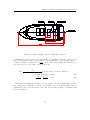
9.6
AX1500 I/O card from RoboteQ . . . . . . . . . . . . . . . . . . . . . . . 126
9.7
Actuator control loop with P controller) . . . . . . . . . . . . . . . . . . . 127
9.8
Step response for a step from -10.5 to 10◦ ) . . . . . . . . . . . . . . . . . . 128
9.9
Step response for a step from -10.5 to 10◦ ) . . . . . . . . . . . . . . . . . . 128
9.10 Implemented heading controller behaviour at 5 knots . . . . . . . . . . . . 130
9.11 Implemented heading controller behaviour at 12 knots . . . . . . . . . . . 130
9.12 Implemented heading controller behaviour at 20 knots . . . . . . . . . . . 131
9.13 Gain scheduling with constant desired heading . . . . . . . . . . . . . . . 132
9.14 Gain scheduling with a step in desired heading . . . . . . . . . . . . . . . 132
9.15 Way-point navigation around Munkholmen, Trondheim . . . . . . . . . . 133
9.16 Way-point navigation with missed waypoint . . . . . . . . . . . . . . . . . 133
9.17 Graphical User Interface (GUI) for the autopilot . . . . . . . . . . . . . . 134
x
11.1 Experiments on a snowy early November morning.... . . . . . . . . . . . . 141
11.2 Lone rider.... . . . . . . . . . . . . . . . . . . . . . . . . . . . . . . . . . . 141
B.1 Input - output sequence at 5 knots . . . . . . . . . . . . . . . . . . . . . . 149
B.2 Measured ROT vs ROT derived from the heading at 5 knots . . . . . . . 150
B.3 Shifted ROT vs ROT derived from the heading at 5 knots . . . . . . . . . 150
B.4 Input - output sequence at 12 knots . . . . . . . . . . . . . . . . . . . . . 151
B.5 Measured ROT vs ROT derived from the heading at 12 knots . . . . . . . 152
B.6 Shifted ROT vs ROT derived from the heading at 12 knots . . . . . . . . 152
B.7 Input - output sequence at 12 knots . . . . . . . . . . . . . . . . . . . . . 153
B.8 Measured ROT vs ROT derived from the heading at 20 knots . . . . . . . 154
B.9 Shifted ROT vs ROT derived from the heading at 20 knots . . . . . . . . 154
C.1 Input/output data, 5 knots Rudder pump experiments . . . . . . . . . . . 155
C.2 Model output, 5 knots Rudder pump experiments . . . . . . . . . . . . . . 156
C.3 Frequency response, 5 knots Rudder pump experiments . . . . . . . . . . 156
C.4 Step response, 5 knots Rudder pump experiments . . . . . . . . . . . . . . 157
C.5 Residuals, 5 knots Rudder pump experiments . . . . . . . . . . . . . . . . 157
C.6 Bode plot, 5 knots Rudder pump experiments . . . . . . . . . . . . . . . . 158
C.7 Pole-Zero plot, 5 knots Rudder pump experiments . . . . . . . . . . . . . 158
C.8 Input/output data, 12 knots Rudder pump experiments . . . . . . . . . . 159
C.9 Model output, 12 knots Rudder pump experiments . . . . . . . . . . . . . 160
C.10 Frequency response, 12 knots Rudder pump experiments . . . . . . . . . . 160
C.11 Step response, 12 knots Rudder pump experiments . . . . . . . . . . . . . 161
C.12 Residuals, 12 knots Rudder pump experiments . . . . . . . . . . . . . . . 161
C.13 Bode plot, 12 knots Rudder pump experiments . . . . . . . . . . . . . . . 162
C.14 Pole-Zero plot, 12 knots Rudder pump experiments . . . . . . . . . . . . . 162
C.15 Input/output data, 20 knots Rudder pump experiments . . . . . . . . . . 163
C.16 Model output, 20 knots Rudder pump experiments . . . . . . . . . . . . . 164
C.17 Frequency response, 20 knots Rudder pump experiments . . . . . . . . . . 164
C.18 Step response, 20 knots Rudder pump experiments . . . . . . . . . . . . . 165
C.19 Residuals, 20 knots Rudder pump experiments . . . . . . . . . . . . . . . 165
C.20 Bode plot, 20 knots Rudder pump experiments . . . . . . . . . . . . . . . 166
xi
C.21 Pole-Zero plot, 20 knots Rudder pump experiments . . . . . . . . . . . . . 166
C.22 Slope R and deadtime Ld of the Ziegler-Nichols step response method at
5 knots . . . . . . . . . . . . . . . . . . . . . . . . . . . . . . . . . . . . . 167
C.23 Slope R and deadtime Ld of the Ziegler-Nichols step response method at
12 knots . . . . . . . . . . . . . . . . . . . . . . . . . . . . . . . . . . . . . 168
C.24 Slope R and deadtime Ld of the Ziegler-Nichols step response method at
20 knots . . . . . . . . . . . . . . . . . . . . . . . . . . . . . . . . . . . . . 169
C.25 Ultimate gain, Ku and period Tu of the Ziegler-Nichols ultimate-sensitivity
method at 5 knots . . . . . . . . . . . . . . . . . . . . . . . . . . . . . . . 170
C.26 Ultimate gain, Ku and period Tu of the Ziegler-Nichols ultimate-sensitivity
method at 12 knots . . . . . . . . . . . . . . . . . . . . . . . . . . . . . . . 171
C.27 Ultimate gain, Ku and period Tu of the Ziegler-Nichols ultimate-sensitivity
method at 20 knots . . . . . . . . . . . . . . . . . . . . . . . . . . . . . . . 171
C.28 ZN ultimate sensitivity vs. step-response at 5 knots . . . . . . . . . . . . 172
C.29 ZN ultimate sensitivity vs. step-response at 12 knots . . . . . . . . . . . . 173
C.30 ZN ultimate sensitivity vs. step-response at 20 knots . . . . . . . . . . . . 173
xii
List of Tables
1.1
Kaasbøll 19 specifications . . . . . . . . . . . . . . . . . . . . . . . . . . .
6
1.2
Evinrude 50 E-tec specifications . . . . . . . . . . . . . . . . . . . . . . . .
6
1.3
Seapath 20 specifications . . . . . . . . . . . . . . . . . . . . . . . . . . . .
9
3.1
Froude number as a planning indicator . . . . . . . . . . . . . . . . . . . . 24
3.2
Froude number and regime at 5, 12 and 20 knots . . . . . . . . . . . . . . 25
7.1
PID parameters . . . . . . . . . . . . . . . . . . . . . . . . . . . . . . . . . 68
7.2
PID parameters obtained from the Ziegler-Nichols step-response method . 69
7.3
P parameters obtained from the Ziegler-Nichols step-response method . . 69
7.4
PID controller parameters obtained from the Ziegler-Nichols ultimatesensitivity method . . . . . . . . . . . . . . . . . . . . . . . . . . . . . . . 70
7.5
PI controller parameters obtained from the Ziegler-Nichols ultimate-sensitivity
method . . . . . . . . . . . . . . . . . . . . . . . . . . . . . . . . . . . . . 72
7.6
P controller parameters obtained from the Ziegler-Nichols ultimate-sensitivity
method . . . . . . . . . . . . . . . . . . . . . . . . . . . . . . . . . . . . . 72
8.1
PID parameters calculated from the Ziegler-Nichols step-response method
8.2
PID parameters calculated from the Ziegler-Nichols ultimate-sensitivity
method . . . . . . . . . . . . . . . . . . . . . . . . . . . . . . . . . . . . . 89
8.3
Controller parameters at 20 knots . . . . . . . . . . . . . . . . . . . . . . . 102
8.4
Controller parameters at 12 and 5 knots . . . . . . . . . . . . . . . . . . . 102
8.5
Input signal properties . . . . . . . . . . . . . . . . . . . . . . . . . . . . . 111
8.6
Output to Simulink . . . . . . . . . . . . . . . . . . . . . . . . . . . . . . . 111
8.7
Operating modes . . . . . . . . . . . . . . . . . . . . . . . . . . . . . . . . 112
8.8
States . . . . . . . . . . . . . . . . . . . . . . . . . . . . . . . . . . . . . . 113
8.9
State hierarchy . . . . . . . . . . . . . . . . . . . . . . . . . . . . . . . . . 113
xiii
86
9.1
Syntax for setting channel 1 and 2 of the AX1500 I/O card . . . . . . . . 125
xiv
Nomenclature
b̄
Proportional set-point weighting complement, b̄ = 1 − b
Z
The Z transform-operator
ŷ
Model output
M
Total mass of the system for calculation of CG
X
X position of the mass for calculation of CG
L
Laplace operator
b
Proportional set point weighting
e(t)
Error value, e(t) = yref (t) − y(t)
K
Proportional gain
mi
Particle masses for calculation of CG
ri
Particle position for calculation of CG
s
Laplace variable
Td
Derivative time
Ti
Integral time
u(t)
Controller output value
ub (t) Proportional reset term
uD (t) Derivative part of controller
uI (t) Integral part of controller
uP (t) Proportional part of controller
y(t)
Measured output value
xv
yref (t) Reference value / set-point value
L−1
Inverse Laplace operator
Ψ0−360 Discontinuous heading measurement from zero to 359◦
Ψcont Continuous heading measurement
τ
Integral variable
A
Amplitude of the input step
c
The derivative set point weighting variable
Cpid (s) Continuous transfer function of the controller model
E(s)
Laplace transform of the error
es
Tracking error
Fn
Froude number
g
Gravity
h
The sampling period
H0−360 (s) Delay due to the discontinuous measurements
HI (s) Continuous transfer function of the integrator
Hlp (s) Continuous transfer function of the reference model
k
The sampling instants k = 0, 1, 2, . . .
L
Overall submerged length of the vessel
Ld
Deadtime of Ziegler-Nichols step-response method
N
Gain limiter for derivative action
q
The shift-operator
R
Steepest slope of Ziegler-Nichols step-response method
Tt
Tracking reset time
U
Vessel speed
UD (s) Laplace transform of the derivative action
UI (s) Laplace transform of the integral action
UP (s) Laplace transform of the proportional action
z
The complex variable of the Z transform
xvi
Acronyms
ASCII
American Standard Code for Information Interchange
CG
Centre of Gravity
DGPS
Differential Global Positioning System
DP
Dynamic Positioning
GPS
Global Positioning System
GUI
Graphical User Interface
IALA
International Association of Marine Aids to Navigation and Lighthouse
Authorities
ITTC
The International Towing Tank Conference
LSE
Least-Square Estimate
LOS
Line Of Sight
MIMO
Multiple-Input Multiple-Output
NMEA National Marine Electronics Association
PD
Proportional-Derivative
PI
Proportional-Integral
PID
Proportional-Integral-Derivative
PRBS
Pseudo Random Binary Signal
RBS
Random Binary Signal
RCP
Rapid Control Prototyping
RMS
Root Mean Square
ROT
Rate Of Turn
xvii
SISO
Single-Input, Single-Output
SNR
Signal to Noise Ratio
USV
Unmanned Surface Vehicle
ARX
Autoregressive eXtra input
FFT
Fast Fourier Transform
xviii
Introduction
Maritime operations have a long and rich history in Norway. Traditionally fishery was
the driving force. With the introduction off-shore oil production the vessel demands
changed and today the off-shore industry is the driving force. Increased complexity,
though environments and expensive operations have lead to an increasing demand for
small, cost effective autonomous vessels. This master thesis is part of a programme
conducted by Maritime Robotics AS to develop a rapid prototyping platform for USVs.
The long term goal of the programme is to develop a fleet of USVss for various operations,
including formation control. These vehicles are envisaged to have significant application
in commercial and naval marine operations in the future.
Areas of interest for naval application includes deployment and pick up of equipment,
mine sweeping, force multiplication, surveys and hazardous operations. Common is the
benefit of removing the human crew and hence reducing human risk. Introduction of
Unmanned Surface Vehicle (USV)s also offer lower life cycle costs and scale benefits in
scaling low-cost USV systems. For commercial use some areas of interest are deployment
and pick up of equipment, rescue operation, surveys, inspection of offshore installations
and seismic surveys. Formation control can reduce the time needed to perform search
and survey operations. Earlier work in the field of USVss includes the American and
Israeli navy (Elbit Systems (2006) and Aeronautics Defense Systems (2006)) as well
as rescue vessels (International Submarine Engineering, 2006) and research projects on
planning vessel dynamics (Ueno et al., 2006).
At present time there are several commercial autopilots on the market from different
producers. Commercial auto pilots are usually delivered with limited information about
the internal aspects of the controllers as this is considered to be business sensitive information. It is important for Maritime Robotics AS to have full access to the details of the
autopilot system as this is one of the foundation of the vessel control system. Therefore
development of their own system is needed.
1
Problem specification
The work in this project thesis have two purposes. The first is aimed at developing and
implementing a heading autopilot for a particular test vessel. This autopilot should be
capable of controlling the heading over the whole range of operating speeds for the vessel,
that is from 0 to 20 knots. The heading autopilot should be easy to tune and have a
small overshoot, no more than ±3◦ in calm water. The autopilot should not experience
oscillatory behaviour. Gain scheduling will be implemented so that the controller can
operate at different speed regimes despite the changing dynamic of the vessel. As an
addition to the heading autopilot a way-point guidance system will be added when the
implementation of the heading autopilot is finished.
The second objective of this thesis is to develop a rapid prototyping environment
for development of USV control systems at Maritime Robotics. This rapid prototyping
environment includes modelling of the vessel and building a vessel simulator in MATLAB/Simulink where new controllers can be developed and tuned before they are implemented in the USVs. This will ease the development of new controllers in projects with
other vessels. The heading controller and way-point guidance system will be developed
in this rapid prototyping environment to gain experience and improve the environment.
Implementation and validation will be done in the test vessel.
Outline of the report
The rest of this report is structured as follows: Part 1 presents necessary background
information. Vessel and equipment configuration is presented in Chapter 1 and some
basic background information on Rapid Prototyping is given in Chapter 2. Part 2 consists of the modelling, where experiment setup is presented in Chapter 3 and system
identification is performed in Chapter 4. The control design and implementation is presented in Part 3. Necessary background on control theory is provided in Chapter 7 while
Chapter 8 presents the controller design in Simulink and finally the implementation is
described in Chapter 9. The results of the previous chapters are discussed in Chapter 10,
after the discussion a proposal for further work is given based on the discussion. Finally
the conclusion of the master thesis and proposals for further work is given in Chapter 11.
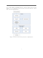
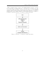
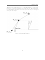
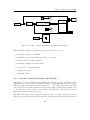
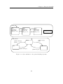
Figure 1 presents the work flow in our master thesis. The initial step is to state the
problem specification before the modelling is commenced. Modelling starts by specifying
and running identification experiments. The results of the experiments are investigated
to see if they provide enough information for the system identification procedure. If
they do not provide enough information they either have to be repeated or re-designed.
Based on the final experiment data, system identification is performed and the resulting
system is analysed to find its performance and limitations. The identified system is later
2
used to build a simulator in Simulink. Then the controller is designed and tested in the
simulator before it is implemented and tested in the vessel. If necessary the controller
will be tuned after implementation.
Figure 1: Work flow from problem specification to implementation
3
Part I
Background
4
Chapter 1
Vessel and Equipment
Configuration
1.1
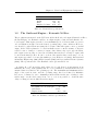
The Vessel - Kaasbøll 19
The test boat, Kaasbøll 19 (Figure 1.1), is a 19 feet planning centre console boat from
a local manufacturer close to Trondheim. This size is well suited because it provides
the capability to carry personnel on board for testing, hence eliminating the need for a
support vessel. It also provides enough space to mount the necessary equipment for a
wide range of tasks and allows for a large fuel tank, providing greater range of operation.
The hull of the boat is constructed in aluminum which is robust and maintance-free.
Finally the boat has a size which permits it to operate in a wide range of sea states.
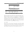
The specifications for the boat is given in Table 1.1.
Figure 1.1: Kaasbøll 19 feet centre console boat, (Kaasbøll Boats AS)
5
Chapter 1. Vessel and Equipment Configuration
Hull
Length
Width
Mass
Displaced volume
5.75
2.12
450
0.45
Unit
m
m
kg
m3
Table 1.1: Kaasbøll 19 specifications
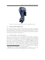
1.2
The Outboard Engine - Evinrude 50 Etec
The propulsion system used on the USV is an off-the-shelf outboard engine, Evinrude 50 E-tec,
shown in Figure 1.2. Evinrude 50 E-tec is a light-weight, robust and fuel-efficient outboard engine. This engine gives the boat a maximum speed of 25 knots with one person
on board which is enough to meet the desired operating range of 10 to 20 knots. However,
care should be taken when increasing the load since this will require a more powerful
engine. If the USV is planned to be used in shallow water or in the vicinity of divers it
would be wise to change to a water jet engine. Since this is only a prototype the Evinrude engine serves it purpose, but it is very likely that another boat and/or engine will
be used in the final product. It can be seen in other articles that a wide range of boat
and engine types have been tried in similar projects; Ebken et al. (2005), International
Submarine Engineering (2006), Elbit Systems (2006) and Aeronautics Defense Systems
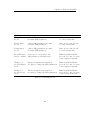
(2006). The specifications for the Evinrude 50 are given in Table 1.2.
A change ∆ of 30◦ in rudder angle takes 2-3 seconds (based on information from
Maritime Robotics). This quantity has not been confirmed by measurement but it is
assumed that it is valid for all operating speeds. The maximum and minimum rudder
angle of the vessel is ±30◦ , and the operating range has been defined by Maritime
Robotics to be limited to ±25◦ . Assuming a linear relation in the rate of change for the
rudder angle over the whole range from −25◦ to +25◦ it is possible to obtain the time
delay for changes between different rudder angles.
Model E50DPL
Mass
Propshaft force @ 5750 rpm
Gear Ratio
Displacement
109
37
2.67:1
863
Unit
kg
kW
cm3
Table 1.2: Evinrude 50 E-tec specifications
6
Chapter 1. Vessel and Equipment Configuration
Figure 1.2: Outboard engine Evinrude 50 E-tec, (Kaasbøll Boats AS)
1.3
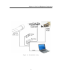
Measurement Equipment
The measurement equipment consists of a Differential Global Positioning System (DGPS)
sensor. The sensor gives measurements to a laptop via the RS232 interface1 . In addition
the Simrad LF3000 provides us with rudder angle measurements. The laptop is used to
give desired control input to the actuator and to run the control algorithms. A schematic
of the measurement setup is given in Figure 1.3.
1.3.1
DGPS Compass - Seatex Seapath 20
The vessel is equipped with a Seatex Seapath 20 GPS Compass (Figure 1.4) which give
heading, position, velocity and rate of turn. Further, the sensor is fitted with an International Association of Marine Aids to Navigation and Lighthouse Authorities (IALA)
beacon receiver to ensure improved position accuracy with DGPS signals. As shown in
Figure 1.4 the Seapath provides RS232 interface to communicate NMEA01832 messages
with the laptop. Both the Global Positioning System (GPS) signals and data from the
gyrocompass is used to calculate heading. This combination provides the heading even
when there is no GPS coverage. In addition we obtain a more accurate heading during
and after turns. GPS measurements can be taken at a maximum frequency of 1 Hz. For
1
The RS232 interface is a standard for serial binary data interconnection between a DTE (Data
terminal equipment) and a DCE (Data Circuit-terminating Equipment)
2
NMEA 0183 protocol is combined electrical and data protocol for communication between marine
electronics. It is defined and controlled by National Marine Electronics Association (NMEA)
7
Chapter 1. Vessel and Equipment Configuration
Figure 1.3: Measurment set-up
8
Chapter 1. Vessel and Equipment Configuration
higher frequencies an interpolated value using the course and speed are calculated. A
short summary of the most important features of the Seapath are given in Table 1.3. For
more details please consult (Kongsberg Seatex AS, 2003, Seapath 20: User’s Manual).
Figure 1.4: Seapath 20 DGPS sensor, (www.km.kongsberg.com)
Seapath 20 GPS compass
Heading accuracy
Rate of turn accuracy
Position accuracy with DGPS
Velocity accuracy with DGPS
0.4
0.5 + 5%
1.5
0.05
Unit
◦ RMS
◦ /s
m RMS
m/s RMS
Table 1.3: Seapath 20 specifications
1.3.2
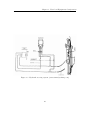
Simrad RPU80 Rudder pump and LF3000 Rudder Sensor
A Simrad RPU80 rudder pump is used to move the outboard engine. This pump is
reversible to provide turning in both direction, and has a capacity of 0.8 l/min. The
direction of the pump is controlled by the polarity of the voltage and the flow rate is
controlled by the voltage level, maximum at 12 V. The maximum power consumption
is 6 A, with an average of 2.4 A (40% of maximum). Moreover, the pump is part of
a hydraulic steering system which in addition to the pump consists of a tiller which
translate the linear motion of the cylinder to a rotary motion of the outboard engine. A
Simrad LF3000 feedback unit is used to measure the cylinder expansion and consequently
the rudder angle. The complete assembly for a vessel with a seperate rudder can be seen
in Figure 1.5.
1.4
Equipment mounting and calculation of CG
We made a some simplifications when calculating the Centre of Gravity (CG). First of all
we omitted the equipment and personnel in the boat because this is variable. Second,
9
Chapter 1. Vessel and Equipment Configuration
Figure 1.5: Hydraulic steering system, (www.simradyachting.com)
10
Chapter 1. Vessel and Equipment Configuration
we calculated the CG with both the outboard engine and the 75 kg gasoline tank as
particle masses. Finally we placed CG from the different components on the same y and
z axes. This simplifies the calculations to only include displacement in the x axis.
The centre of mass R of a system of particles is defined as the average of their positions
ri , weighted by their masses mi :
R=
X=
1 X
mi ri
M
1
(1.25 m × 75 kg + 2.32 m × 109 kg) = 0.55 m
(109 + 75 + 450) kg
(1.1)
(1.2)
where M is the total mass of the system, equal to the sum of the particle masses.
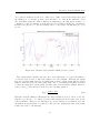
The CG of the boat alone, the engine and the fuel tank are shown in Figure 1.6 and
Figure 1.7. Using (1.1) we find the CG of the complete assembly, also shown in the
above mentioned figures which are CAD drawings obtained from the manufacturer and
modified with their permission.
Figure 1.6: CAD drawing of the boat with CG, sideview
11
Chapter 1. Vessel and Equipment Configuration
Figure 1.7: CAD drawing of the boat with CG, overview
Changing the load on the boat will change its dynamics and CG. Our project
has been performed with 2 persons in the boat, resulting in a total weight change of
2 × 80kg = 160kg or an increase of 160kg
634kg = 25%. The corresponding CG with the persons loacted close to the centre console is given as:
X=
1
(1.25 m × 75 kg + 2.32 m × 109 kg + · · ·
(109 + 75 + 450 + 160) kg
1.00 m × 160 kg) = 0.64 m
∆x
64 − 55
=
= 1.6%
length
5.75
(1.3)
(1.4)
This change is significant in change of total weight, but just a small change in CG.
If we change the configuration even more by adding 2 more persons including 50 kg of
equipment to the boat 1 m in front of the CG, an even larger change of dynamics will
be noted as shown:
12
Chapter 1. Vessel and Equipment Configuration
X=
1
(1.25 m × 75 kg + 2.32 m × 109 kg + · · ·
(109 + 75 + 450 + 320 + 50) kg
1.00 m × 160 kg − 1.00 m × 210 kg) = 0.64 m
(1.5)
30 − 55
∆x
=
= 4.4%
(1.6)
length
5.75
These changes of 4.4% in CG and 370kg
634kg = 58% in total weight compared to an empty
boat are significant, and the controller should be tuned according to load or be designed
very robust.
13
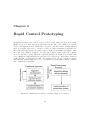
Chapter 2
Rapid Control Prototyping
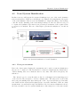
We will in this chapter give a short overview of the concept of Rapid Control Prototyping
(RCP) and how we have used it in this master thesis. The goal of RCP is to rapidly
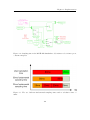
develop and implement new designs and concept in controller design. Traditional and
rapid prototyping approach to solving a control problem is illustrated in Figure 2.1.
The traditional approach needs a large team of engineers in multiple disciplines. First
the control algorithm is designed. Secondly the software team creates the software
needed to run the program. Then the requested hardware is designed by another team
before finally the implementation is performed by a last group. Rapid Prototyping is
a different way of solving the problem. The main idea is to let the computer software
automatically transfer high level code to a real-time program using built in compilers
and communication libraries.
Figure 2.1: Traditional vs rapid prototyping design of a controller
14
Chapter 2. Rapid Control Prototyping
A wide variety of programs have been used for rapid prototyping. We have in this
thesis used MATLAB Simulink models with extensions to StateFlow block diagrams.
Theses tools provides us with an easy to use and intuitive interface for designing and
tuning the controller. An example of this could be the task of extending the controller
to include anti-windup. In Simulink this is simply done by adding some blocks to our
model. Traditional approach on the other hand would demand changes to the C-code of
the program and maybe also implementation of new drivers and measurement routines.
A possible flow of the rapid prototyping process can be found in Figure 2.2.
2.1
Simulator
When testing out a new design it is very convenient to not work directly on the plant,
both with regards to cost and time consumption. If the computer simulates the process
to be controlled, fast simulation which could take ten times as much time on the real
process can be performed in a few minutes. To be able to do these simulations, we
need to make a model of the process to be controlled. This is done in Chapter 4. A
mathematical model is then used to represent the “real process”. It is never possible
to exactly identify all the dynamics of the process, but nevertheless the simulations will
give us a good starting point.
2.2
Real-time constraints
Normally when performing rapid prototyping, a real-time system is provided. Often
running on a real-time operating system such as VxWorks, QNX or MATLAB xPC.
During this development both the desired operating system and final hardware was
undecided. So because of limited time, a “almost real-time” solution was used. Our
solution uses a windows PC and MATLAB with Simulink. To control the time of the
simulations, a free ware block designed by Daga (2007). The information given below is
a summary of the description found on the homepage of Daga (2007).
The RT Blockset for Simulink consists of a block using a S-function written in C++
language. It can not be compared to running the simulations on a real time operating
system since it does not use a separate OS or runs a real-time kernel. This blockset is
based on the simple concept that, to make the Simulink run with a real-time approximation, the calculation time neded by Simulink should be lower then the desired simulation
step. If this assumption is not valid, no real-time simulation is possible, whichever is the
applied scheduling method. This assumption is not completely valid since windows is
not a real-time OS and has other processes running on the same time. If another process
with higher priority takes up all the calculation time of the system, we will have error
in the calculated values of Simulink.
15
Chapter 2. Rapid Control Prototyping
Figure 2.2: The flow of a rapid prototyping process
16
Chapter 2. Rapid Control Prototyping
This block simply holds the execution of the Simulink simulation attached to the time
flow, leaving whatever remaining CPU time to other windows processes that need it. The
concept is very simple but effective. Another approach would be to use the MATLAB
real time workshop and the real-time windows target kernel. But these toolboxes are a
relatively large cost for a small company, so at the moment they were not available to
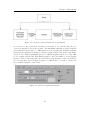
us. Figure 2.3 shows the structure of our rapid prototyping environment.
Figure 2.3: Structure of our rapid prototyping environment
17
Part II
Modelling
18
Chapter 3
Experiments
This chapter will introduce important concepts for design of system identification experiments, and design of experiments to identify models of a small USV will be performed.
These models will be implemented in a computer simulator where they will be used in
the design of a heading controller and in analysis of the control system.
3.1
Input design for open loop experiments
Performing experiments on physical systems are costly and time consuming, therefore
it is important to design experiments which are as informative as possible to reduce
these factors. By informative experiments we mean experiments that excites all relevant
dynamics of the system and enables us to chose the best model candidate. This is
called a rich signal. Ljung (1999) defines an informative experiment as: “An open
loop expreiment is informative if the input is persistently exciting”. The mathematical
definition of a persistently exciting signal can be found in Definition 13.1 in Ljung (1999).
A signal A(t) is persistently exciting of order n, if its spectrum is different from zero on
at least n points in the interval −π < ω < π.
In order to use Matlab and Simulink in the development of the heading controller we
need an accurate model of the vessel. Based on the experience gained in Beinset and
Blomhoff (2006), the experiments have been updated and improved in order to develop
a satisfying model. Analysis in Beinset and Blomhoff (2006) suggested that the Binary
Rudder manoeuvre provided the best data set for the system identification procedure
and that this manoeuvre should be used for system identification. Figure 3.1 outlines
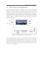
the experiment set-up with the vessel and the computer for set-point control and logging.
A LabView interface enabling computer control of the input and logging was developed
to remove the human operator and improve the logging (see Figure 3.2). Set-points
19
Chapter 3. Experiments
Figure 3.1: Set-up for system identification experiments
are read from a file by Labview and imposed as input to the system using the zero
order hold principle between the updates. The maximum sampling frequency with the
current hardware was found to be 4 Hz during previous experiments. At higher sampling
frequencies the hardware is having problems providing reliable data as the temperature
drops below 0◦ . With a sampling frequency of 4 Hz the Nyquist frequency becomes 2 Hz,
see for example Åström and Wittenmark (1997) for more information on the Nyquist
frequency. It is worth noting that the vessel and steering dynamics of the vessel will act
as a low-pass filter and a Nyquist frequency of 2 Hz should be enough to capture the
most essential dynamics of the vessel.
Figure 3.2: LabView application interface
20
Chapter 3. Experiments
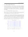
3.2
Binary Rudder Manoeuvre
The Binary Rudder Manoeuvre consists of using a Pseudo Random Binary Signal (PRBS)
as set-point for the rudder angle of the vessel and then logging the Rate Of Turn (ROT)
and the input signal. This input - output relationship is used to identify the dynamics
between the input and the output, as explained in detail in Chapter 4. The input signal
and its properties are important when performing experiments to do system identification. In the next section we will elaborate the properties of the Pseudo Random Binary
Signal (PRBS).
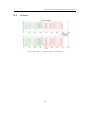
3.2.1
Pseudo Random Binary Signal properties
This section describes the properties of a PRBS and the justification for using this as an
input signal. First some general information on PRBS are provided, then the properties
of the actual PRBS sequence used in this experiment is analysed.
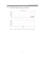
A PRBS is a periodic, deterministic signal with white-noise like properties. The signal
can attain two values, ±U. Here U is the value of the signal. The PRBS sequence was
created off-line using the idinput(length,’prbs’) function in Matlab. Here length gives
the sequence length and ’prbs’ sets the signal type to a PRBS. The PRBS changes
between two values, ±1. The sequence is scaled so that it provides the correct rudder
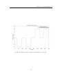
set-point before it is imposed. A part of the PRBS sequence can be seen in Figure 3.3
(the complete sequence is to long to be plotted on a page). By creating the signal off-line
it is possible to investigate it in advance to ensure its properties.
Figure 3.3: Part of a PRBS sequence with a length of 255
21
Chapter 3. Experiments
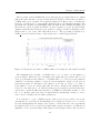
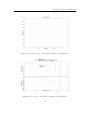
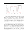
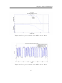
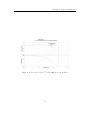
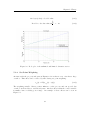
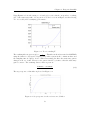
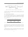
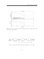
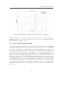
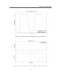
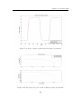
The spectrum of an ideal PRBS has a very flat frequency spectrum, that is, it contains
almost the same amount of energy at all frequencies. Figure 3.4 shows the spectrum of
a PRBS with a period length of 255 which is sampled at 1 Hz, it can be seen that the
frequency content is more or less equally distributed up to the Nyquist frequency. The
spectrum was calculated in MATLAB, using the Fast Fourier Transform (FFT) and
the methods of Periodograms and Welch. A periodogram is a power spectral density
estimate, while Welch is averaged periodograms of overlapped, windowed signal sections.
Welch tends to give a smoother PSD when plotted. The spectrum is calculated by
PRBS spectrum.m and the usage of this script can be found in Appendix A.1.
Figure 3.4: Frequency spectrum of a PRBS with period length 255 and sampled at 1 Hz
The maximum period length of a PRBS is M = 2n − 1, where n is the number of
previous inputs. When the period is finished the signal will repeat itself. The second
order properties(mean and variance) of a PRBS will be good as long as the signal is
evaluated over an integer number of periods. By averaging the output over the periods
from such a signal one will improve the signal to noise ratio by a factor of i, where i
is the number of periods. At the same time the data to handle in the analysis will be
reduced by the same factor. A drawback with periodic signals in general is that they
can at most contain M different frequencies. A PRBS is persistently exciting of order
M − 1, see (Ljung, 1999, Page 421). A signal which is persistently exciting of order n
can be used to identify a model with n parameters.
It is desirable to create a PRBS sequence that is as long as possible, but as the
experiments are performed in Trondheimsfjorden at high speeds the need of obstacle
free surroundings limits the length of the sequence. At the first run of the experiments
the signal described above was used as input with a update frequency of 1 Hz and an
amplitude of ±15◦ in rudder angle. This sequence had a length of 1023. The experience
22
Chapter 3. Experiments
gained from this run was that the steering hydraulics and the vessel dynamics were to
slow to react to the changes in the input and the frequency of update should be reduced.
As the rudder machinery is able to make rudder changes at a maximum rate of 6◦ /s it
was decided to update the input every third second and reduce the amplitude to ±8◦ .
This ensures that the actual rudder angle set-point can be imposed before another setpoint is given. It is assumed that the change in ROT is linear with the change in rudder
angle. Decreasing the update frequency is the same as increasing the clock period, see
(Ljung, 1999, page 422), and the sequence length had to be reduced due to the increased
clock period.
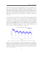
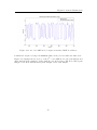
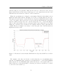
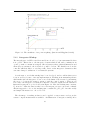
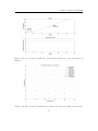
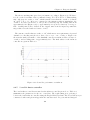
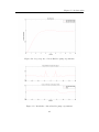
The new input was updated with a frequency of 0.33 Hz and the sequence length was
255. The length of 255 was chosen to get a full sequence, the next full PRBS sequence
has a length of 511, which is to long at 20 knots. It will take approximately 13 min
to complete a sequence with 255 values. At 20 knots this corresponds to a maximum
travelled distance of approximately 8 km. This signal will be persistently exciting of
order M − 1 = 254, (Ljung, 1999, Page 421). A possible threat to the experiment is
other vessels which might lead to an aborted experiment to avoid a possible collision.
The first half of the resulting data is to be used for model calculation while the second
half is to be used for validation. From Figure 3.5 it can be seen how the increased clock
period changes the spectrum(compare Figure 3.5 to Figure 3.4).
Figure 3.5: Frequency content of a PRBS input sequence updated at 0.33 Hz
This effect is described in Ljung (1999) on page 422. Ljung (1999) suggest sampling the
system about 10 times faster than the bandwidth of the system to be modelled. With a
sampling time of 4 Hz it implies that we should have models with a bandwidth which is
less than 0.4 Hz. Figure 3.5 shows that the frequencies up to approximately 0.3 Hz are
well exited. So the input signal is the limiting factor in this experiment and it is limited
by the steering hydraulics.
23
Chapter 3. Experiments
Since the dynamics of the vessel changes with the speed, it was decided to do models at
different speeds to account for these changes. It is normal to define three different regions
for the dynamic of a vessel moving in water with respect to the speed. These regions
are displacement, semi-displacement and planning. In this report we will define them as
a function of the Froude number. For a comprehensive discussion on this subject, see
Beinset and Blomhoff (2006), Chapter 2.1. The Froude number is defined as:
Fn = √
U
L×g
(3.1)
Where U is the vessel speed, L overall submerged length of the vessel and g is gravity.
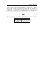
Table 3.1 gives the three regimes as a function of the Froude number.
Region
Diplacement
Semi displacement
Planning
Froude number
F n < 0.4
0.4 < F n < 1.0 − 1.2
F n > 1.0 − 1.2
Table 3.1: Froude number as a planning indicator
24
Chapter 3. Experiments
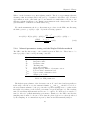
The Binary Rudder Manoeuvre was performed at 5, 12 and 20 knots, these velocities
are chosen so that the experiments covers displacement, semi-displacement and planning
motion, see Table 3.2.
Speed
5
12
20
Froude number
0.34
0.82
1.37
Operating area
Displacement
Semi-displacement
Planning
Table 3.2: Froude number and regime at 5, 12 and 20 knots
25
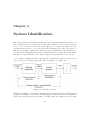
Chapter 4
System Identification
The ideal conditions for running experiments for the system identification would be an
indoor facility where the current, waves and wind could have been controlled and set
to zero. As our vessel is a full scale vessel, this is not a realistic alternative and the
experiments have therefore been performed in Trondheimsfjorden. As a consequence of
this, the test results contains wave wind and current disturbances. Experiments were
performed in Trondheimsfjorden on the 21. March 2007, the weather was sunny with a
wind speed of approximately 1 m/s. Wave height was approximately 0 cm to 30 cm.
As both the commanded rudder angle and the actual rudder angle is logged we can
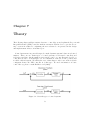
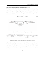
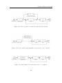
choose between two different approaches when identifying, see Figure 4.1.
Figure 4.1: Systems to identify
The first possibility is to identify the dynamics from actual rudder angle to ROT, this will
identify the dynamics of the vessel. By identifying the system between the commanded
rudder angle and the actual rudder angle one will identify the dynamics of the steering
26
Chapter 4. System Identification
hydraulics. The second possibility is to identify the system from commanded rudder
angle to ROT, resulting in a system which covers both the dynamics of the vessel and
the steering hydraulics. These experiments uses the AC20 autopilot interface and the
rudder machinery is controlled by AC20. This means that the steering hydraulic is a
closed loop system including dead band non-linearities introduced by the controller from
Simrad. The intention is to replace the AC20 controller, therefore it is preferable to do
the system identification for the vessel and the steering hydraulic separately.
First the steering hydraulic system identification will be presented, then the system
identification of the vessel dynamics. Throughout this chapter models are tested and
validated against real data from sea trials with the USV. The percentage of fit is defined
as:
ky − ŷk
F it = 1 −
× 100%
(4.1)
ky − mean(y)k
Here y is the output of the vessel, ŷ is the model output and mean(y) is the average
of the vessel output. The fit tells us how much of the vessels behaviour that can be
explained by the model.
The scripts used for data treatment and analysis can be found on the CD enclosed
at the end of this report and the content of this CD is listed in Appendix D. Also the
system identification sessions are present, these can be loaded into MATLAB system
identification toolbox. The usage of these scripts can be found in Appendix A.
27
Chapter 4. System Identification
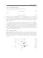
4.1
Rudder Pump System Identification
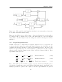
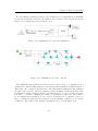
In this section we will present the system identification process of the steering hydraulics
and the built in Simrad P-controller, see Figure 4.2. This model is used for designing
the heading controller in Simulink. An advantage with this solution is that it offers
flexibility to try out different methods off-line and later implement them using a rapid
prototyping environment. Since the dynamics of the pump are not very complicated,
we chose a simple first-order model structure to represent its behaviour. We will give
a detailed report on the 20 knots model identification, and just give the results and
deviations for the 5 and 12 knots model since the procedure is the same. For a more
detailed presentation on the system identification, please consult Beinset and Blomhoff
(2006) and Ljung (1999).
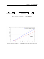
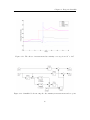
Figure 4.2: System identification of steering hydraulics
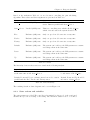
A square-input experiment done on the boat was used as basis for this system identification. The results of this experiments are shown in Figure 4.3 and gives us the pump
behaviour with the integrated Simrad P-controller. It is important to note that this
model, which represent both the pump and the integrated Simrad P-controller, will be
replaced by an analog voltage out card with a new controller design during the implementation on the vessel. But nevertheless, this model will aid us in the first controller
design phase done in Simulink.
28
Chapter 4. System Identification
Figure 4.3: Rudder pump behaviour with Simrad P-controller
29
Chapter 4. System Identification
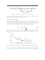
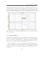
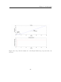
4.1.1
20 knots model
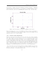
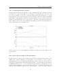
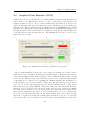
We use the MATLAB System Identification toolbox and divides the measured data into
an estimation part and a validation part as shown in Figure 4.4. The identification
are performed, and suitable ARX models are calculated as shown in Figure 4.5. For
residuals, frequency response and step response figures, please consult Appendix C. Our
goal was to find a simple and suitable model. The 1st order ARX model gives about 85
% fit, and the 4th order ARX model gives almost 90 % fit. We decide to use the simple
1st order because of its simple structure and satisfactory behaviour.
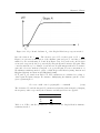
Figure 4.4: Rudder pump range for estimation and validation at 20 knots
The obtained 1st order ARX model with time delay has the structure given as:
δ(k)
0.1562
=
q −2
δref (k)
1 − 0.8447q −1
(4.2)
where δ(k) is the rudder angle, and δref (k) is the desired rudder angle at sample k.
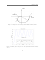
The obtained model for 20 knots has a pole-zero plot as seen in Figure 4.6 and the
Bode plot with phase and gain margins can be found in Figure 4.7. Poles can be found
30
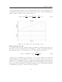
Chapter 4. System Identification
Figure 4.5: Rudder pump model output at 20 knots
in z = 0 and z = 0.8447, and since they have an absolute value of less than one, we
can conclude that the model is stable. Moreover we see that the phase margin is equal
to 172◦ and the gain margin 16.1 dB, which confirms our conclusions of a steady model
from the pole-zero plots. The cut-off frequency at 0.108 Hz is lower and gives slower
dynamics than the actual system as can be seen from Figure 4.5, but this only results
in a more robust system. We therefore conclude that the model is good enough for the
relatively slow dynamics of the pump.
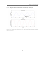
4.1.2
5 and 12 knots models
The identification of the 5 and 12 knots models follow the same procedure as given above
and detailed plots can be found in Appendix C. Equations for the models are given as:
δ(k)
δref (k)
δ(k)
δref (k)
=
=
0.1485
q −2 5 knots model
1 − 0.8530q −1
0.1555
q −2 12 knots model
1 − 0.8458q −1
(4.3)
(4.4)
Both of these models are stable. In addition we can see that the models performs very
similar as seen in Figure 4.8. This leads us to conclude that the rudder pump system
31
Chapter 4. System Identification
Figure 4.6: Pole-zero plot of the rudder pump model at 20 knots
Figure 4.7: Bode plot of the rudder pump model at 20 knots
32
Chapter 4. System Identification
is more or less independent of the velocity of the boat. From the same figure we see
that the 20 knots model performs best on the 20 knots data. This is also the case for 12
and 5 knots data. We therefore conclude that the 20 knots model should be used on all
velocities since it gives the best performance. Finally it should be noted that this model
includes a closed loop controller in addition to the hydraulic system. The closed loop
controller is a rate limited p-controller with dead zone non linearities. However as the
system is a fairly simple and it is believed that the new controller design will behave in
a similar way, this model is used to simulate the steering hydraulics.
Figure 4.8: Model output of the rudder pump model at 20 knots with different speed
models
33
Chapter 4. System Identification
4.2
Vessel System Identification
In this section we will present the system identification process of the vessel dynamics
from actual rudder to ROT as seen in Figure 4.9. This model is implemented as a part
of the vessel simulator that is created in Simulink for design and tuning of the heading
controller. As the dynamics of the vessel changes with speed, three models are developed
to capture the dynamics. The first section presents pre-treatment of the acquired data
to prepare it for analysis. The rest of this chapter presents the analysis at 5, 12 and 20
knots.
Figure 4.9: System identification of vessel dynamics
4.2.1
Data pre-treatment
Before the data acquired during the experiments can be used for system identification
they need to be inspected. The data should be checked for high-frequency disturbances,
outliers, missing data, non-continuous data records, drift, offset and low-frequency disturbances.
The data is logged to a text file with one line for each sample and a visual inspection
of the text file was performed to check for missing data. The inspection revealed that
there was some missing GPS data, namely the course on ground and the speed information. ROT and the actual rudder signal did not experience this kind of fall out. Only
measurement of actual rudder angle and ROT are used for system identification, hence
the data can still be used for system identification. After inspection of the raw text file
34
Chapter 4. System Identification
containing the logged data, it is imported into Matlab with the script import− data.m
(see Appendix A.2 for usage of this script).
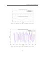
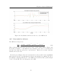
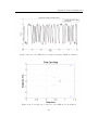
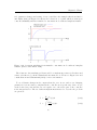
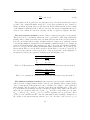
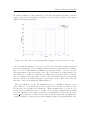
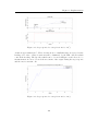
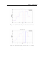
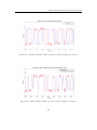
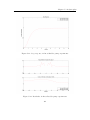
Visual inspection of the ROT reveals that the measured ROT is having a time delay. This was first seen when the rudder angle and the ROT was plotted together, see
Figure 4.10.
Figure 4.10: ROT and actual rudder angle plotted together
In Figure 4.10 the two data points correspond to the same point in time and it can
be seen that the measured ROT is delayed by approximately 36 s. The derivative of
the heading measurement was then derived and it was compared to the rudder angle
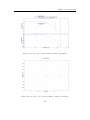
measurement, see Figure 4.11. The derivative was implemented as:
s
s
=
τs + 1
0.5s + 1
(4.5)
Here τ determines the upper frequency included in the derivative. τ equals 0.5 and this
value was chosen based on the Nyquist-frequency which is 2 Hz.
The derivative of the heading can be used in the identification procedure, but the
derivative contains a high level of noise as can be seen in Figure 4.11. Instead of using
the derivative for system identification it was used to adjust the time delay in the ROT
measurements, which have a lower noise level than the derivative.
35
Chapter 4. System Identification
Figure 4.11: ROT derived from heading and actual rudder angle plotted together
The heading sensor is providing heading data in the range [0◦ - 360◦ ] and the signal
will not be continuous when the heading goes from 360◦ to 0◦ or the other way around.
This will result in a very large derivative as the heading goes from the maximum to
the minimum value in two samples. Therefore it was necessary to convert the ROT
measurement to a signal in the range ± inf, this conversion makes the heading measurement continuous. The conversion is done by parseLabViewLog.m as the data is loaded
in MATLAB. Usage of this function can be found in Appendix A.3(parseLabViewLog.m
is called by import− data.m). This section provides a comprehensive presentation of
the data adjustment at 5 knots, while the adjustment at 12 and 20 knots is given in
Appendix B. The procedure for the adjustment is the same at all three speeds.
Figure 4.12 shows the ROT derived from the heading and the measured ROT at 5 knot
plotted together. This Figure clearly show the delay of the measured ROT. The delay
was found after identifying a distinct shape which both the calculated and the measured
ROT contained, this is where the data cursors are placed in the plot of Figure 4.12. The
time delay was found to be 5.7 s, which corresponds to 23 samples as the sampling rate is
4 Hz. Based on these results, the sequence containing the measured ROT was shifted 23
samples, so that the 23rd sample became the first sample. The shifted sequence is plotted
again together with the ROT derived from the heading in Figure 4.13. The figure shows
that the measured and calculated ROT is very similar. The figure clearly shows that
the calculated ROT contains more noise than the measured ROT. The measurement
of the actual rudder had to be cut at the end so that the two data sequence had the
same length. The Delay at 5 knots was, as mentioned, 5.7 s, at 12 knots the delay was
36
Chapter 4. System Identification
35.5 s and at 20 knots it was 8.5 s. There is no buffer between the GPS sensor and
the COM-port on our laptop, hence there should be no delay in the hardware. It is
also unexplained why the delay is different at different speeds, although it seems to be
constant for each experiment even though the speed changes during the experiment.
LabView is believed to be the most likely source of the delay, but this have not been
proved.
Figure 4.12: Measured and calculated ROT plotted together
The output signal contains some noise due to wave disturbance, to reduce the influence
of waves it was decided to filter the signal before the analysis. Filtering the signal
introduces a phase shift, therefore it is important to filter both the input and the output
signal so that they have the same phase shift. A 1st order Butterworth filter was used
to filter the input and output signal, the filter was created with the Matlab function,
butter(order,ωn ). The filter is described by the following equation:
L(q) =
0.22q + 0.22
q − 0.56
(4.6)
In Figure 4.14 the unfiltered ROT and the filtered ROT is plotted. Most of the disturbance is believed to be caused by waves with frequencies in the same area as the
vessel dynamics. Therefore pre filtering done on the dataset is very limited and only
the highest frequencies have been filtered. The plot also displays the time delay which
is introduced due to the filtering.
37
Chapter 4. System Identification
Figure 4.13: The measured ROT shifted 23 samples and plotted together ROT derived
from the heading
Figure 4.14: Filtered and unfiltered ROT
38
Chapter 4. System Identification
4.2.2
5 knots model identification
The input - output data at 5 knots consist of a sequence of approximately 13 mins.
The set point is changed every third second and data is logged at a frequency of 4 Hz.
The first 7.5 mins are used for model calculation while the rest of the signal is used for
validation, see Figure 4.15. The time delay in the ROT measurement was 5.7 ss so this
measurement was shifted 23 samples and 23 samples was deleted from the end of the
input sequence to obtain equal length for the two sequences.
Figure 4.15: Model input and outputs at 5 knots
An impulse response model, frequency response model, 4th order Autoregressive eXtra
input (ARX) model, with time delay, and a state space model was calculated in the
system identification toolbox using the Quick Start option. After calculating the models
they are validated against input - output data from the vessel. The model is then
subject to the same input as the one used in the vessel and the output of the model is
compared with the behaviour of the real vessel. The initial analysis gave a fit of 70.4%
for the State Space model while the ARX model obtained a fit of 68.9%, see Figure 4.16.
Further analysis led to a 10th order ARX model, which yield a fit of 73.2%.
Investigating the residuals of three models in Figure 4.17 it can be seen that the
autocorrelation of the residuals are smaller for the two ARX models are small than for
the 4th order state space model. It should be noted that the residuals of the 4th and 10th
39
Chapter 4. System Identification
Figure 4.16: Model outputs at 5 knots
order ARX are similar, with the 10th order residuals being slightly smaller than the 4th
order ARX model.
As the fourth order ARX models have a simple structure and are found to perform
almost as well as higher order models and more complicated models, they are chosen as
the preferred models. In this section it is seen that fit of the three models presented differ
by 4.3%, this is not a significant difference. This information combined with information
from the residuals indicate that one of the ARX models should be chosen. The 4th order
model is chosen due to its simplicity and because this results in the same model structure
for the models at 5, 12 and 20 knots. The details for the 4th order model is presented
below.
4.2.3
Best model at 5 knots
The ARX model with time delay is given as:
r(k)
0.04955 − 0.04301q −1 + 0.01898q −2 − 0.01659q −3
=
× q −2
δ(k)
1 − 2.771q −1 + 3.009q −2 − 1.539q −3 + 0.3117q −4
(4.7)
Where r(k) is the ROT and δ(k) is the rudder angle. k is the sample number. The
output of the models response to the validation data is plotted together with the vessels
response in in Figure 4.18, where it can be seen that the model gives a realistic output.
Most of the deviation between the model and the real output is believed to be caused
by disturbance in the measurement, for instance wave motion.
40
Chapter 4. System Identification
Figure 4.17: Residuals of the 4th order ARX model at 5 knots
Figure 4.18: Model output of 4th order ARX model at 5 knots
41
Chapter 4. System Identification
Poles and zeros of this model is plotted in Figure 4.19. The model has 6 roots(marked
with an x) inside the unit circle(two at origo) and three zeros(marked with an o), hence
the model is stable, but it is a non-minimum phase system because of the time delay.
Figure 4.19: Poles and zeros of the 4th order ARX model at 5 knots
Figure 4.20 displays the bode plot of the ARX model. The model has a gain margin of
9.09 dB at 0.395 Hz while the phase margin is infinite as the model is damped for all
frequencies and does not cross the 0 dB line.
4.2.4
12 knots model identification
The same set-up is used for the 12 knot model as for the 5 knot model, that is, sampling
time of 0.25 s and the set-point is changed every 3rd second. The first 4.6 min are used
for calculation while the rest is used for validation. The total length of the input - output
sequence is approximately 12 min. The sequence can be found in Appendix B.2. As for
the 5 knots data this data-set also suffered of a time delay in the ROT measurement. The
data at 12 knots had a delay of 35.5 s, which is a very large delay. The ROT measurement
had to be shifted 142 samples and the last 142 samples of the input had to be deleted.
Adjustment of the ROT measurement at 12 knots can be found in Appendix B.2.
As for the 5 knot model, Quick Start was used to identify an impulse response model,
frequency response model, 4th order ARX model and a state space model. Figure 4.21
shows the performance of the different initial models.
42
Chapter 4. System Identification
Figure 4.20: Bode plot for the 4th order ARX model at 5 knots
Figure 4.21: Bode plot for the 4th order ARX model at 5 knots
43
Chapter 4. System Identification
The initial analysis gave a fit of 85.6% for the State Space model while the ARX
model obtained a fit of 82%. Figure 4.21 also displays the performance of an 10th order
ARX model which was calculated to see how much it was possible to improve the model.
The improvement compared to the 4th order model is very small. Figure 4.22 shows the
residuals of the three models and these residuals are fairly similar and does not provide
information to discriminate between the models.
Figure 4.22: Residuals at 12 knots for the 4th order ARX model
Due to the simplicity of the ARX model and because the performance of the State Space
model is only 3.6% better, we chose to continue using the ARX model. More details on
this model is presented below.
4.2.5
Best model at 12 knots
The ARX model is given as:
r(k)
0.0233 − 0.0875q −1 + 0.2585q −2 − 0.1752q −3
=
δ(k)
1 − 2.613q −1 + 2.732q −2 − 1.391q −3 + 0.2914q −4
(4.8)
Figure 4.23 shows the output of the ARX model compared to the measured behaviour
of the vessel.
Investigating the poles and zeros of the system, reveals that the system is a nonminimum phase system as two of its zeros are placed outside the unit circle. The system
44
Chapter 4. System Identification
Figure 4.23: 4th order ARX model output vs measured ROT at 12 knots
is still stable despite it being non-minimum phase as its poles are inside the unit circle.
Figure 4.25 displays the Bode-plot of the 4th order ARX model, the gain margin and
phase margin is also marked together with the cut-off frequency. The model has a gain
margin of 3.8 dB at 0.48 Hz and a phase margin of 112◦ at 0.186 Hz.
45
Chapter 4. System Identification
Figure 4.24: Poles and zeros for 4th order ARX model at 12 knots
Figure 4.25: Bode plot for the 4th order ARX model at 12 knots
46
Chapter 4. System Identification
4.2.6
20 knots model identification
As for the 5 and 12 knots models, the sampling time is 0.25 s and the set-point is changed
every third second. The first 7.5 min are used for calculation while the rest is used for
validation. Total length of the input - output sequence is approximately 12.5 min, this
sequence can be found in Appendix B.3. Time delay at 20 knots was found to be 8.5 s,
hence the ROT measurement sequence was shifted 34 samples, so that sample 34 became
the first sample. The 34 last samples was also deleted from the input. Adjustment of
the ROT measurement at 20 knots can be found in Appendix B.3.
Figure 4.26 shows the performance of the State Space model and the ARX model which
was found by Quick Start in the System Identification toolbox. This figure reveals that
the models at 20 knots produces an output which is almost identical to the output of
the vessel when they are subject to the same input. It is believed that the difference to
a great extent is created by waves and measurement noise. This behaviour was found
to be so good that it was not put any effort in finding better models. The state space
approach and the ARX yields almost identical results, where the State Space model have
a fit of 90.6% and the ARX model has a fit of 89.6%.
Figure 4.26: Model outputs at 20 knots
The residuals of the two models are also similar, as seen in Figure 4.27. As for the 12
knots model it is difficult to use the residuals to discriminate between the two models.
The ARX model was chosen due to its simplicity and to obtain a unified model structure
for the models at 5, 12 and 20 knots.
47
Chapter 4. System Identification
Figure 4.27: Residuals at 20 knots for the 4th order ARX model
4.2.7
Best model at 20 knots
The ARX model is given as:
0.03435 − 0.1124q −1 + 0.3695q −2 − 0.2131q −3
r(k)
=
δ(k)
1 − 2.328q −1 + 2.413q −2 − 1.354q −3 + 0.3388q −4
(4.9)
Where r(k) is the ROT and δ(k) is the rudder angle. k is the sample number. Figure 4.28
shows the performance of the ARX model at 20 knots, as it can be seen this model
perform better than the models at 5 and 12 knots. This is in accordance with the
discussion in Section 4.2.3
From the plot in Figure 4.29 it is clear that the model is a stable but non-minimum
phase system. It is also clear that the models at 12 and 20 knots are similar. The Bode
plot in Figure 4.30 shows that the 4th order ARX model at 20 knots have a phase margin
of 56.4◦ at 0.305 Hz. The cut-off frequency is 0.71 Hz.
48
Chapter 4. System Identification
Figure 4.28: 4th order ARX model output vs measured ROT at 20 knots
Figure 4.29: Poles and zeros of the 4th order ARX model at 20 knots
49
Chapter 4. System Identification
Figure 4.30: Bode plot of the 4th order ARX model at 20 knots
50
Chapter 5
Discussion
To simplify the reading of the report this part will end with a discussion of the modelling
and the results obtained. The discussion is presented below, while the conclusion of the
modelling process is presented in the next chapter.
During the experiment design in Chapter 3 it was found that we should be able to
identify models with a bandwidth up to 0.3 Hz. The analysis of Chapter 4 resulted with
a bandwidth of the 5 and 12 knots which are less than 0.15 Hz while the bandwidth
of the 20 knots model was found be 0.71 Hz. This indicates that the input signal and
the sampling frequency is well chosen for the 5 and 12 knots model, while they are not
optimal for the 20 knots model. With the present system this is the best alternative,
as the experiments where limited by the steering dynamics and the sampling rate. A
possible improvement of the experiments at 20 knots would be to implement a larger
pump with faster dynamics. Then it would be possible to change the input signal at a
higher rate and the bandwidth could be increased. Then the sampling rate would become
the limitation and it should be increased as well to further increase the bandwidth to
improve the experiments at 20 knots.
The introduction to the system identification mentioned that the vessel is subject to
environment disturbances. The data from different trials are influenced differently as
they are performed at different points in time. This means that the conditions might
change from one experiment to another. The speed of the vessel also influences the
impact of the environmental disturbances. When the vessel is at low speed its motion
will be strongly influenced by waves and wind. Increasing the speed of the vessel will
increase the relative frequency of incoming waves and the dynamics of the vessel will
not be able to follow the fast motion of small waves hitting the hull. The result is that
the motion of the vessel will be less influenced by waves. Therefore increasing the speed
has the effect of moving the wave spectrum towards higher frequency area. The result
of this is that more of the wave motion will be filtered out by the dynamics of the vessel
51
Chapter 5. Discussion
which is acting as a low pass filter. This effect is believed to cause most of the observed
improvement in the model accuracy with respect to real output data from the vessel
which increases from 68.9% at 5 knots to 89.6% at 20 knots.
When the experiments were designed, it was assumed that the relationship between
ROT and rudder angle is linear. In Figure 5.1 it can be seen that this is not the case.
The figure plots the real rate of turn and the model predicted ROT when rudder angles
of ±15◦ are applied. The model gives a lower steady state ROT than the real system
and the result is a steady state error. As the steady state error occurs in the ROT it
will not affect the heading, but the real system will be faster than the model. When
tuning the controller based on this model, it might result in a larger gain than the
optimal. Therefore it might be necessary to reduce the gain of the controller when it is
implemented in the vessel.
Figure 5.1: Deviation between measured ROT and model predicted ROT at 15◦ rudder
angle
The analysis of the three models also revealed that they are non-minimum phase
systems. Non-minimum phase systems are generally harder to control than minimum
phase system. In a non-minimum phase system the inverse of the system will not be
stable as the zeros of the system then becomes its poles, therefore it will not be possible
to use it in a feed forward loop.
52
Chapter 5. Discussion
Different models where identified at all three speeds and three ARX models where
chosen even though other models gave a marginal improvement in some cases. The
ARX models was chosen as they have a simple structure and are easy to implement in
a computer. It is also a advantage that all three models have the same structure.
53
Chapter 6
Conclusion
A vessel model and Steering hydraulics, including a feedback controller, has been identified and modelled. The steering hydraulic model is given as a first order model with
time delay:
δ(k)
0.1562
=
q −2
δref (k)
1 − 0.8447q −1
(6.1)
where δ(k) is the rudder angle, and δref (k) is the desired rudder angle at sample number
k.
The vessel identified is a planning monohull vessel. Dynamics of the vessel was divided
into three regimes: displacement, semi displacement and planning. Three models was
identified at 5, 12 and 20 knots. Corresponding to the displacement, semi displacement
and planning regimes respectively. The three models are ARX models with the following
structure:
5 knots model which yields a fit of 68.9%:
r(k)
0.04955 − 0.04301q −1 + 0.01898q −2 − 0.01659q −3
=
× q −2
δ(k)
1 − 2.771q −1 + 3.009q −2 − 1.539q −3 + 0.3117q −4
(6.2)
Here r(k) is the ROT and δ(k) is the rudder angle at sample k.
12 knots model which yields a fit of 82%:
r(k)
0.0233 − 0.0875q −1 + 0.2585q −2 − 0.1752q −3
=
δ(k)
1 − 2.613q −1 + 2.732q −2 − 1.391q −3 + 0.2914q −4
(6.3)
20 knots which yields a fit of 89.6%:
r(k)
0.03435 − 0.1124q −1 + 0.3695q −2 − 0.2131q −3
=
δ(k)
1 − 2.328q −1 + 2.413q −2 − 1.354q −3 + 0.3388q −4
54
(6.4)
Chapter 6. Conclusion
The complete system from desired rudder angle to heading yields the following ztransform to be used in simulations:
ψ(k)
(0.1562)(0.03435 − 0.1124z −1 + 0.3695z −2 − 0.2131z −3 )
K × Ts
=
z −2
−1
−1
−2
−3
−4
δref (k)
(1 − 0.8447z )(1 − 2.328z + 2.413z − 1.354z + 0.3388z )
z−1
(6.5)
Here
K×T s
z−1
is the discrete integrator from ROT to heading.
55
Part III
Control Design
56
Chapter 7
Theory
The following chapter will give an introduction to control theory and explain the ProportionalIntegral-Derivative (PID) controller with its extensions. This is done to give the necessary overview in addition to explaining the more advanced concepts used in the design
and implementation later on in this report.
Control systems are in general designed to make dynamic systems behave in a desired
manner. There are two main types of control systems, feed-forward controllers and
feedback controllers. Another name is respectively open-loop controllers and closed-loop
controllers as can be seen in Figure 7.1. A combination of the two is also possible and
is called a hybrid system. We will in the rest of this chapter only focus on the feedback
configuration since the PID controller is of this type. For more information on basic
control theory, please consult Balchen et al. (2003).
Figure 7.1: General types of control systems
57
Chapter 7. Theory
Here y(t) is the measured output, yref (t) is the desired reference value, e(t) is the error
(e(t) = yref (t)−y(t)) and u(t) is the controller output. The process is here also assumed
to include both the actuator which applies u(t) on the system and the sensors which
measure y(t).
7.1
PID control
The PID controller is by far the most known and used controller. According to Åström
and Hägglund (1996b), about 90 to 95% of all control problems are solved by this
controller. A reason for its widespread use is its simple structure and robustness to
a large number of common control problems. In the early days of the PID controller,
it was implemented using relays, electric motors or pneumatic or hydraulic systems.
Later the systems were replaced by electronics and nowadays integrated ciruits are used
to implement flexible and powerful digital solutions. As stated by its name, the PID
controller consists of a proportional part, an integral part and a derivative part. These
different components each provides important features and we will in the rest of this
chapter have a detailed look at them and their posssible extensions. The following
equation:
u(t) = uP (t) + uI (t) + uD (t)
(7.1)
and Figure 7.2 presents one configuration of the PID controller, the parallel repersentation, and it clearly shows the three different parts of the system. Here u(t) is the control
output, uP (t) the propartional part, uI (t) the integral part, uD (t) the derivative part
and e(t) the error (e(t) = yref (t) − y(t)).
Figure 7.2: Parallel representation of the PID controller
58
Chapter 7. Theory
7.1.1
Proportional Control
The proportional control is a simple feedback given as:
uP (t) = Ke(t)
(7.2)
e(t) = yref (t) − y(t)
(7.3)
where
Here K is a proportional gain and e(t) is the error which is defined to be the difference
between the desired reference value, yref (t), and the measured output value, y(t). The
toilet bowl floating proportioning valve is an example of a pure proportional controller.
As the water in the tank rise, the floating element also rise and gradually close the valve
filling up the tank.
A problem with the proportional controller is that it tends to have a steady-state
error. This steady state error appears because when the error is zero, the controller
only provides the steady state control action for the original steady state which could
be different from the new set point. To get the system to operate near the new steady
state, the controller gain, K, must be very large so the controller will produce the required output. Having large gains can lead to system instability or can require physical
impossibilities like infinitely large valves.
7.1.2
Integral Control
A manually adjustable reset term was added to the control signal to remove the steadystate error of the proportional controller. Integral action was a result of trying to develop
automatic tuning of this reset term. The idea was to filter out the low frequency part of
the error signal and add it to the control output as shown in Figure 7.3 and the following
equations:
u(t)
=
uP (t) + ub (t)
(7.4)
L[. . .] m
U (s)
=
U (s)
=
(7.5)
KE(s) + Ub (s)
1
K(1 +
)E(s)
sTi
L−1 [. . .] m
=
u(t)
=
(7.7)
(7.8)
Z
u(t)
(7.6)
t
K
e(τ )dτ
Ti
uP (t) + uI (t)
Ke(t) +
59
(7.9)
(7.10)
Chapter 7. Theory
Figure 7.3: Controller with integral action / automatic reset
This shows us that the automatic reset with a low pass filter on a proportional controller
is the same as a Proportional-Integral (PI) controller.
7.1.3
Derivative Control
A negative effect of the integral control is that it introduce a phase lag of 90◦ . This
means that some systems might turn unstable due to integral action. Derivative control
on the other hand gives us a 90◦ phase lead. Derivative action can therefore be seen as
a prediction. A Proportional-Derivative (PD) controller can be presented as:
u(t) = uP (t) + uD (t)
de(t)
u(t) = K(e(t) + Td
)
dt
(7.11)
(7.12)
Equation 7.12 shows that derivative control is actually a Td time units linear look-ahead
predictor for the error, e(t). Figure 7.4 gives a informative visual interpretation of the
derivative action.
Figure 7.4: Derivative action interpreted as prediction, (Åström and Hägglund, 1996b)
Because of its phase lead of 90◦ as shown in Figure 7.5, derivative control is often used
to increase the gain or gain margin of the proportional control. However, caution must
60
Chapter 7. Theory
be taken when using derivative action on systems with have piecewise constant set point
or significant measurement noise. The derivative part of the controller will then give
infinite output according to the following equations:
uD (t) = KTd
dyref (t) dy(t)
de(t)
= KTd (
−
)=∞
dt
dt
dt
(7.13)
Figure 7.5: 90◦ phase lead of the derivative action
Limited derivative action
To counteract this effect, the derivative gain is often limited by filtering it through a low
pass filter. In practice this means it is only limited to a gain of N at high frequencies.
N is normally chosen to be in the range 3 to 20. This realization is given as:
UD (s) = sTd E(s) ⇒ UD (s) =
KTd s
1+
sTd
N
E(s)
(7.14)
This can also be illustrated by plotting the bode plot of the derivative part with and
without limitation as seen in Figure 7.6. Here we see that the gain is very low at low
frequencies for the unlimited version, but that the gain keeps rising as the frequency
increases. For steps this will result in an infinite gain. When limiting the gain by setting
N=10, we get the green line labelled “Limited derivative action”. The gain is now limited
to 20dB which correspond to 10 as given in the following:
61
Chapter 7. Theory
20 ∗ log10 (value) = decibel value
(7.15)
m
20
Decibel to absolute value:10 20
= 10
(7.16)
Figure 7.6: Bode plot of the unlimited and limited derivative action
7.1.4
Set Point Weighting
An issue with the proportional part in Equation 7.2 is that it very often has a large
overshoot. This effect can be reduced by introducing set point weighting:
uP (t) = K(byref (t) − y(t))
(7.17)
The weighting variable b has a positive influence on the process, and can provide less
overshoot and less delay to reach steady state. Another effect is that the control variable
is smaller, hence reducing power usage. An example of these effects can be seen in
Figure 7.7.
62
Chapter 7. Theory
Figure 7.7: The usefulness of set point weighting, (Åström and Hägglund, 1996b)
7.1.5
Integrator Windup
The integral part of a PID controller is stable in a closed loop, but turns unstable when
it is opened. This is due to the integrator element which would tend to infinity in an
open-loop with a constant at its input. All real actuators have physical limitations and
when they are saturated, the feedback loop will be broken. The unstable mode in the
controller will then drift to a very large value. Later, as the integrator desaturates, this
can cause damped oscillations or even unstable systems.
Several ways to avoid this windup have been developed, and we will in this section
focus on tracking because of its easy implementation. Tracking is an antiwindup scheme
which makes sure the integrator does not exceed the limits of the actuator by measuring
the error, es , between the actuator output, u, and the control output, v. This error is
feed back to the integrator, resetting it so that the controller output is at the saturation
limit and keeping the loop closed as seen in Figure 7.8. Here the tracking time constant,
Tt , is used to define the time it takes before the integrator is reset. As a rule of thumb
Åström suggested to choose the tracking time constant T d ≤ T t ≤ T i. Another widely
used simple alternative is to choose T t = T i.
The advantage of tracking is that it can be applied on any actuator as long as the
actuator output measurement is available. An illustration of integrator windup effect
63
Chapter 7. Theory
Figure 7.8: A PID controller with tracking antiwindup, (Åström and Wittenmark, 1997)
and the system with windup protection is given in Figure 7.9.
Figure 7.9: Effects of a PID controller with and without antiwindup, (Åström and
Wittenmark, 1997)
7.1.6
Bumpless transfer
Bumpless transfer describes the objective of avoiding transients when changing the properties of the controller. These changes can be switching from manual to automatic con64
Chapter 7. Theory
trol, parameter changes and testing of new controllers. An example taken from Graebe
and Ahlén (1996) in Figure 7.10 shows the behaviour of a plant which at start-up is
controlled manually and later switched to automatic mode without bumpless transfer.
Figure 7.10: A system switching from manual to automatic mode without bumpless
transfer, (Graebe and Ahlén, 1996)
The solution to the switching problem would be to implement positive feedback around
a first-order filter for both the manual and automatic mode. Please see Figure 7.11 and
consult Åström and Wittenmark (1997) for more information.
To avoid drastic changes in the output when the error is zero and we are changing
parameters, it is necessary to implement the controller in a specific way. Since we are
at the desired set point and the error is equal to zero, the active part of the controller
is the integral action. The two different implementations used to describe the problem
are given as:
Z
K t
I =
e(τ )dτ
Ti
Z t
K(τ )
I =
e(τ )dτ
Ti (τ )
65
(7.18)
(7.19)
Chapter 7. Theory
Figure 7.11: PID controller with bumpless switching between manual and automatic
mode, (Åström and Wittenmark, 1997)
Equation 7.18 will here give a sudden jump or bump in the integral action when there
are changes in K Ti . Equation 7.19 on the other hand will give a smooth bumpless
change in the controller output because the changes are added to the integrator and not
multiplied.
7.1.7
Digital Implementation
All PID controllers to be implemented on digital computers need to be discretised due
to the fact that all computers are inherently sampled systems. Since the PID controller
originally was an analog invention, a discrete approximation is used. The three basic
methods for approximation are the forward difference (or Euler method), the backward
difference method and the Tustin’s method (also called the bilinear method). Their
approximations are given as:
dx(t)
≈
dt
dx(t)
≈
dt
dx(t)
≈
dt
q−1
h x(t),
Z⇒ z−1
h X(z)
Forward difference
(7.20)
q−1
qh x(t),
Z⇒ z−1
zh X(z)
Backward difference
(7.21)
Tustin’s approximation
(7.22)
2 q−1
h q+1 x(t),
Z⇒
2 z−1
h z+1 X(z)
Here q is the shift operator defined as qx(t) = x(t + h) and h is the sampling period.
Z defines the Z transform as given in Proakis and Manolakis (1996). A mapping of the
stability region in the s-plane to the z -plane for the three approximations are given in
66
Chapter 7. Theory
Figure 7.12. With the forward difference it is then possible to map a stable continuoustime system to an unstable discrete-time system. For the backward difference method
on the other hand, every mapping of a stable continuous-time system will also give a
stable discrete-time system. Tustin’s approximation has the advantage that it maps a
stable continuous-time system exactly onto the unit disc, but often also gives a more
complex expression. Care must therefore be taken when choosing the correct method
for discretisation.
Figure 7.12: Mapping of the stability region in the s-plane to the z -plane, (Åström and
Wittenmark, 1997)
The proportional part of the controller can easily be discretised by replacing the
continuous variables with the sampled ones as given by:
uP (t) = K(byref (t) − y(t) ⇒ uP (kh) = K(byref (kh) − y(kh)
(7.23)
Where k defines the sampling instants k = 0, 1, 2, . . ., and kh the total time.
The integral part can be discretised in several ways, but the most common one (as
given in Åström and Hägglund (1996b) and Åström and Wittenmark (1997) is the forward difference approximation:
Z
uI (t) =
t
K
Kh
e(τ )dτ ⇒ uI (kh + h) = uI (kh) +
e(kh)
Ti
Ti
(7.24)
Moreover, the derivative part is approximated by taking the backward differences:
dy(t)
Td duD (t)
+ uD (t) = −KTd
⇒ uD (kh) = · · ·
N dt
dt
nonumber
Td
KTd N
uD (kh − h) −
(e(kh) − e(kh − h))
Td + N h
Td + N h
67
(7.25)
(7.26)
(7.27)
Chapter 7. Theory
Where c is the derivative set point weighting variable. The above approximation has the
advantage that it is always stable and gives good results for all values of Td . Forward
approximation on the other hand can become unstable for small values of Td due to the
mapping explained in Figure 7.12. Tustin’s approximation is also always stable, but can
give undesirable oscillations for small values of Td .
We can then summarise the above discretisation procedure for the PID controller using
the shift-operator, q −1 x(kh) = x(kh − h) in the following equation:
Kh q −1
(yref (kh) − y(kh)) + · · ·
Ti 1 − q −1
KTd N
1 − q −1
e(kh)
(7.28)
Td
−1
Td + N h 1 − T +N
q
h
d
uP ID (kh) = K(byref (kh) − y(kh)) +
7.1.8
Manual parameter tuning and the Ziegler-Nichols methods
The PID controller has a range of free variables given in Table 7.1. These have to be
tuned properly to have a well performing controller.
Variable
K
Ti
Td
Tt
b
N
umin
umax
h
Description
Proportional gain
Integration time
Derivative time
Tracking time
Set point weighting
High frequency limiter of derivative action
Lower actuator saturation level
Upper actuator saturation level
Sample period time
Table 7.1: PID parameters
The high frequency limiter of the derivative action, N , can be fixed and is typically set
in the range 3-20. Moreover, the saturation limits, umin and umax , should be set close to
the true saturation limits. b, the proportional set point weighting is set to a value in the
interval 0-1 depending on the desired performance as given in Figure 7.7. The tracking
time, Tt is in many implementations chosen to be equal to Ti . If allowed, it can also be
tuned to allow for optimal antiwindup performance. Further, for the PID controllers the
sampling time h must be chosen so short that the phase lead is not adversely affected
by the sampling. A recommendation given by Åström and Wittenmark (1997) is:
68
Chapter 7. Theory
hN
≈ 0.2 to 0.6
Td
(7.29)
The parameters K, Td and Ti are strongly affected by each others and should be tuned
together. Two classical heuristic methods to decide these parameters were defined by
Ziegler and Nichols (1942). They are known as the Ziegler-Nichols methods and consists
of the ultimate-sensitivity method and the step-response method. Originally they were
developed for continuous controllers, but they can also be applied to digital controllers.
The step-response method is a method where a unit step is applied on the system.
This is an open-loop experiment, which can often be performed on-line. Especially in the
industry where a shut-down may cause big financial losses this is the preferred method.
It is also used much when security measures makes it dangerous to push the system
to its stability limits as demanded from the ultimate-sensitivity method, for example in
weapons and nuclear plants. The plants need to have a step response which is essentially
monotone except from an initial non-minimum phase characteristic. K, Ti and Td are
then found in Table 7.2 for the PID controller, and in Table 7.3 for the P controller. R
here denotes the tangent of the steepest slope of the step response, A the amplitude of
the input step and Ld the apparent deadtime as shown in Figure 7.13.
Parameter
K
Ti
Td
Tuned value
1.2×A
R×Ld
2 × Ld
0.5 × Ld
Table 7.2: PID parameters obtained from the Ziegler-Nichols step-response method
Parameter
K
Tuned value
1×A
R×Ld
Table 7.3: P parameters obtained from the Ziegler-Nichols step-response method
The ultimate-sensitivity method or the frequency response method which it is also
called, is based on simple characteristics of the process dynamics. These characteristics
can be found and the PID parameters can be calculated according to desired gain and
phase margin. The key idea is to find the point where the Nyquist curve of the open
loop system intersects with the negative real axis (see Figure 7.14). This point describes
where the process has a phase lag of 180◦ , ω180 , and the corresponding process gain,
K180 = |G(iω)|. K180 and ω180 can be found by applying pure proportional control
on the process, and increase the controller gain until we have standing oscillations on
the output of the system with the ultimate gain , Ku . Because of the closed loop, we
69
Chapter 7. Theory
Figure 7.13: Slope R and deadtime Ld of the Ziegler-Nichols step response method
1
have the relation Ku = K180
. The ultimate period, Tu , is then given by Tu = ω2π
.
180
Figure 7.15 gives us an illustration of the ultimate gain and period. Another point is
marked by arrows indicating P, I and D in Figure 7.14. It describes the effects when
we increase respectively the proportional (P), integral (I) and derivative (D) gain. This
coincides with theory, for example by an increase in gain margin with more derivative
gain, and a decrease with more integral or proportional gain. For more information on
the ultimate-sensitivity method, please consult Ziegler and Nichols (1942), Åström and
Hägglund (1996a) and Åström and Hägglund (2006).
K, Ti and Td are found from Table 7.4. The parameters are calculated according to
desired gain and phase margin. For instance, multiplying the ultimate gain Ku by 0.6
gives a gain margin of:
Ku × 0.6 = 0dB + 20 × log10 (0.6)dB = −4.4370dB
(7.30)
The derivative, Td , and the integral, Ti , parameters adjust the phase margin by changing
the frequency where respectively the derivative and integral action are applied.
Parameter
K
Ti
Td
Tuned value
0.6 × Ku
Tu
2
Tu
8
Table 7.4: PID controller parameters obtained from the Ziegler-Nichols ultimatesensitivity method
70
Chapter 7. Theory
Figure 7.14: Nyquist curve and the Ziegler-Nichols ultimate-sensitivity method
Figure 7.15: Ultimate gain, Ku and period, Tu of the Ziegler-Nichols ultimate-sensitivity
method
71
Chapter 7. Theory
Parameter
K
Ti
Tuned value
0.45 × Ku
Tu
1.2
Table 7.5: PI controller parameters obtained from the Ziegler-Nichols ultimatesensitivity method
Parameter
K
Tuned value
0.5 × Ku
Table 7.6: P controller parameters obtained from the Ziegler-Nichols ultimate-sensitivity
method
7.2
Reference model
Heading set-points should consist of feasible set points for the vessel. A step in the
desired heading would generate a set-point to the vessel which is not achievable, therefore
a reference model is introduced to ensure feasible heading set-points. The reference
model is realised as a second order low-pass filter which is designed based on the vessel
dynamics. A second order filter with two common poles have the following structure:
1
y(s)
k
=
u(s)
(1 + T s)2
(7.31)
Here T denotes the poles, k1 gives the stationary value of the filter and is set to 1. The
time response of a second order filter with two real and common poles, T, exposed to a
step can be expressed as follows:
y(t) =
t
1
t
[1 − ( + 1)e− T ]
k
T
(7.32)
If we set y(t) equal to a desired percentage of the final value of a unit step and rearrange
Equation 7.32 it is possible to design the filter where one can decide the time constant,
at which the filter should output the desired percentage of the final value. The time
constant t should be based on the vessel dynamics and should reflect how fast the vessel
can change its heading. Setting k1 equal to 1 Equation 7.32 in yields:
t
(1 − y(t)) × T
> e− T
t+T
(7.33)
The desired value of y(t) and t are set. Then the functions of the inequality in Equation 7.33
can be plotted as functions of T. From this plot T can be found graphically (see
Figure 7.16). The value of T should be chosen close to the point where the two graphs
intersects, if not the system will be faster than specified.
72
Chapter 7. Theory
Figure 7.16: Determination of T
7.3
Gain Scheduling
The vessel dynamics are dependent of the speed of the vessel and changes with the speed.
Due to these changes it is necessary with different tuning of the controller at different
speeds. This is solved by gain scheduling, where the parameters are adjusted as the
speed of the vessel reaches threshold values for parameter changes. In situations where
the operating point of the vessel is close to a threshold for parameter change, one might
experience oscillation between the parameters. Hysteresis is introduced when switching
parameters to prevent such oscillation. Finally, to avoid steps in the controller when the
parameters are updated, filtering of the parameters are needed so that smooth changes
are obtained.
7.4
Way-Point Navigation System
The route of a ship can be defined by a set of way-points. These way-points defines
points that the boat should pass on its route. The way-point navigation system provides
the heading autopilot with the desired heading.
Line-Of-Sight Guidance Line Of Sight (LOS) is a popular method for creating the
desired path between different way-points. The most basic realisation of this method
sets the LOS vector as the vector between the vessel position(N(t),E(t)) and the next
way point(Nw ,Ew ). Set-point for the heading autopilot can then be found as (see also
Figure 7.17):
ψd = atan2(Ew − E(t), Nw − N (t))
73
(7.34)
Chapter 7. Theory
The function atan2 yields values from −π to π, and this values have to be mapped into
the range 0◦ to 360◦ as this is the input to the heading autopilot. The desired heading
set-point is then filtered through the reference model (see Section 8.1) before it is applied
as set-point to the autopilot.
Figure 7.17: Line-Of-Sight Navigation
74
Chapter 8
Design in Simulink
One of the goals in this report was to design and implement a heading controller on an
Unmanned Surface Vehicle (USV). This design was performed in two steps. First the
controller was developed in the MATLAB Simulink environment. Second, the required
adjustments were done during the implementation. In addition, a reference model was
designed to provide the controller with feasible set points for the vessel. The Rapid
Control Prototyping (RCP) tools of the Simulink environment provided us with great
flexibility when trying out new solutions and possibilities. Moreover, this environment
saves time and is one of the main reason we managed to do everything form system identification to design and implementation in only one Master assignment. The environment
will also offer a base for further development by Maritime Robotics AS.
8.1
Reference model
Based on theory presented in Section 7.2 a second order low-pass filter is designed for
the reference model. The reference model presented in this section is a simple reference
model which is designed so that it is possible to use the same reference model over the
whole range of operating speeds.
To find the limitations of the vessel a rudder angle of 25◦ was set as input to the rudder
pump model in series with the vessel model as seen in Figure 8.1. It is also noticed that
the largest change in set-point that can be experienced is a step of 180◦ as the autopilot
always chooses the shortest path when the heading is changed.
Plotting the time response of the heading as in Figure 8.2 it is seen that the 5 knot model
is the slowest model, and hence this model is the one limiting the reference model. It
is also seen that it takes the 5 knot model approximately 15 s to perform a 180◦ turn.
Based on this observation the time constant is chosen as 15 s.
75
Chapter 8. Design in Simulink
25
Desired rudder angle
0.1562
z2-0.8447z
Actual rudder angle
Rudder Pump
w/ Simrad controller
0.03435z4-0.1124z 3+0.3695z 2-0.2131z
z4-2.328z3+2.413z 2-1.3540z+0.3388
Vessel dynamics 20 knots
ROT
K Ts
Heading
z-1
Discrete-Time
Integrator
Figure 8.1: Desired rudder angle to heading simulation
Figure 8.2: Heading response for 5, 12 and 20 knot models with a rudder angle of 25◦
76
Chapter 8. Design in Simulink
Using Equation 7.33 and setting t = 15 and y(t) = 0.95, which corresponds to reaching
95% of the stationary value of a step in 15 s, it can be seen from Figure 8.3 that chosing
T = 2.5 would yield a satisfying performance.
Figure 8.3: Plot for finding T
1
The resulting filter is given as y(t) = (1+2.5s)
2 . This filter is then discretized in MATLAB
using the function c2d(system,sampling time) where system is the continuous filter and
the sampling time is equal to 0.25 s. When discretizing the filter the stationary gain is
changed from 1 to 1.041. Therefore the gain is divided by 1.041 so that the stationary
gain becomes 1. The resulting discrete filter is given as:
0.004495z + 0.004205
z 2 − 1.81z + 0.8187
The step-response of this filter is plotted in Figure 8.4
Figure 8.4: Step-response for the reference model filter
77
(8.1)
Chapter 8. Design in Simulink
In Figure 8.5 the ROT of the system in Figure 8.1 is plotted for the three models at 5,
12 and 20 knots. The limiting factor here is the 5 knot model which have a maximum
ROT of approximately 20◦ /s. Therefore a rate limiter which limits the ROT to 20◦ /s
is introduced after the filter to limit the derivative so that the desired ROT is feasible.
The complete system in Simulink can be seen in Figure 8.6
Figure 8.5: Model response at 5, 12 and 20 knots to a step in rudder angle of 25 degrees
1
psi_setpoint
0.004495z+0.004205
z2-1.81z+0.8187
Rate Limiter1
1
psi_d
Discrete
2.order filter
Figure 8.6: Final reference model for the heading set-point
8.2
Heading Controller
In Beinset and Blomhoff (2006) a scheme for doing experiments and system identification
on a small USV was created. These experiments were further improved in Chapter 3. We
78
Chapter 8. Design in Simulink
will in this section use the obtained models from the system identification of Chapter 4 to
design and tune a heading autopilot for the USV. The models were validated and tested
to be stable and in coherence with the behaviour of the real vessel in the above mentioned
chapter. These models give us the USVs behaviour from commanded rudder angle to rate
of turn. The two models are divided into a first-order model representing commanded to
actual rudder angel and a fourth-order model giving the behaviour from actual rudder
to rate of turn. Adding an integrator, we have a complete model from desired rudder
angle to heading for the controller design in Simulink as shown in Figure 8.7. The firstorder model will be replaced by the pump and an analog voltage out card with our
own controller when implemented in the vessel. Design in this section are based on the
identified models and not our pump controller to save time in the development process.
For more information on the obtained models, please consult Chapter 4.
Figure 8.7: The model from commanded rudder angle to heading in MATLAB Simulink
We have chosen the PID controller design for our heading controller. This design is a
well known and by far the most used, hence it suits our needs in this project where time
is of an essence. Furthermore, it has a simple structure and good robustness to a large
number of common control problems by implementing different extensions. This simple
structure also suits the needs of Maritime Robotics which have requested an intuitive
basis for further development. The PID controller was also originally developed on the
basis of watching the helmsman steering a ship, taking both oscillatory and constant
disturbances as waves, currents and wind into account. The reason that we have to
include integral action in the controller and not only implement a simple P or PD
controller even though the plant contains integral action, is that some disturbance enter
the plant before the integration as shown in Figure 8.8. This constant disturbance which
affects the boats rate of turn can for example be wind or non linearities in the boat.
When we apply a desired heading of 100◦ , Figure 8.9 shows the steady state error created
by the disturbance.
79
Chapter 8. Design in Simulink
Figure 8.8: Simulink model of the system with a P controller and rate of turn disturbance
Figure 8.9: Steady state error with and without disturbance for a P controller
80
Chapter 8. Design in Simulink
8.2.1
Discontinuous heading measurement (0◦ -359◦ )
The Simulink model in Figure 8.7 consists of a model which give a continuous heading
output. This is not the case for the real vessel. We therefore need to modify the output
of the model to give a heading reading from zero to 359◦ . Figure 8.10 shows how this
discontinuous output are calculated. This block is placed in the block representing the
USV system as shown in Figure 8.11. The equation of the calculations performed in
above mentioned block are:
Ψ0−360 = f loor(
Ψcont
) × 360
360
(8.2)
Figure 8.10: Discontinuous heading output (0-359◦ )
Figure 8.11: USV model with discontinuous heading output (0-359◦ )
We now have a heading measurement from 0 − 359◦ which creates new problems to be
handled. First of all, it is natural that the controller chooses the fastest way to reach its
set point, even when this implies crossing the boundary between zero and 359◦ . Logic to
detect which turning direction is the shortest was created and implemented in Simulink
as a series of if expressions given in Figure 8.12-8.15. These blocks can be interpreted
as follows:
81
Chapter 8. Design in Simulink
1
2
3
4
5
6
7
psi ref
%desired heading
psi
%measured heading
if (abs(psi ref − psi) ≤ 180)
% no need to cross the boundary, psi and psi ref are passed through the
% Simulink block
psi = psi;
psi ref = psi ref;
8
9
10
11
12
13
elseif (psi ref − psi > 180)
% the controller should cross the boundary from 0 to 359, and the
% desired heading should be subtracted 360
psi = psi;
psi ref = psi ref − 360;
14
15
16
17
18
19
20
elseif (psi ref − psi < −180)
% the controller should cross the boundary from 359 to 0, and the
% desired heading should be added 360
psi = psi;
psi ref = psi ref + 360;
end
Figure 8.12: Upper level of the Simulink if block to choose the shortest direction
With these if loops implemented in front of the heading controller in Simulink, the
shortest direction is always chosen. But when crossing the boundary, discontinuities appear in the heading measurement which makes sudden changes in the controller output.
This can be seen in Figure 8.16 where the discontinuity makes the system unstable on a
step from 50◦ to 340◦ . If we run the simulation again, now with a set point further away
from the boundary, we see that an oscillation is introduced by the crossing. Figure 8.17
82
Chapter 8. Design in Simulink
Figure 8.13: Lower level of the first Simulink if block
Figure 8.14: Lower level of the first Simulink if block
Figure 8.15: Lower level of the first Simulink if block
83
Chapter 8. Design in Simulink
shows this oscillation together with the proportional-, integral and derivative controller
output. As seen, the especially the derivative action has a large step due to the sudden
change in heading measurement.
Figure 8.16: The effects of measurement discontinuity on a step from 50◦ to 340◦
To avoid this discontinuity, we decided to add a block between the heading output and
the controller which detects discontinuities and remember how many times the boundary
has been crossed. This number is multiplied by 360 and added to both the set point
and measurement as shown in Figure 8.18. The block which does this transfer from
discontinuous to continuous output has one sample time delay in its memory element,
hence one sample time delay must be added to the measurement and set point entering
into the controller. A small degradation of performance is the result of the delay, but
this can be removed by tuning the PID parameters.
The block which detects the discontinuities needs to be initialised with the correct
value. This is to avoid having the memory element detect a false step when we start
the autopilot at a heading larger than 180◦ . With an initial value of 0, the if loops
in Section 8.2.1 will falsely detect a crossing. To avoid this, measurements are taken
before the simulations are started and given to the simulation as shown in the StartButton Callback function of U SV simulationGui.m given in Appendix A.8. Finally the
complete assembly to handle the 0-360 discontinuity is placed as shown in Figure 8.19.
84
Chapter 8. Design in Simulink
Figure 8.17: The effects of measurement discontinuity on a step from 50◦ to 270◦
Figure 8.18: Simulink block removing the discontinuity in measurement and set point
85
Chapter 8. Design in Simulink
Figure 8.19: Placement of the block to handle the 0-360 discontinuity
A detailed description of the tuning and controller design will be presented for the
20 knots model. For the 5 and 12 knots controllers, only the final parameters and its
performance will be given.
8.2.2
Ziegler-Nichols experiments
A step-response Ziegler-Nichols experiment was performed on the vessel model in Simulink
for 5, 12 and 20 knots as explained in Section 7.1.8. A MATLAB script, ZNstepResponse.m, was designed and used for simulation and calculation of the step-response
parameters. It can be found in Appendix A.5. The results of the 20 knots experiment
can be seen in Figure 8.20.
By using the equations given in Table 7.2, the PID parameters are given as:
Parameter
K
Ti
Td
5 knots value
0.36161
7.9068
1.9767
12 knots value
0.41795
5.7833
1.4458
20 knots value
0.3773
5.6342
1.4086
Table 8.1: PID parameters calculated from the Ziegler-Nichols step-response method
As seen from the table above, the parameters for the 12 and 20 knots controller are
similar. This is also showed in Figure 8.21 where Kp, Ti and Td are plotted together
for all speeds. Therefore it might be possible to use the same parameters at 12 and 20
knots. In addition, it might be useful to do more models in the range 5 to 12 knots in
the future.
When tuning systems according to the Ziegler-Nichols method, we have two possibilities. They are the step-response method performed above, and the ultimate-sensitivity
method. Both approaches are explained in Section 7.1.8.
86
Chapter 8. Design in Simulink
Figure 8.20: Slope R and deadtime Ld of the Ziegler-Nichols step response method at
20 knots
Figure 8.21: Kp, Ti and Td parameters for all speeds derived from ZN step response
87
Chapter 8. Design in Simulink
For the ultimate-sensitivity method, the parameters were implemented in Simulink
models given in Figure 8.22-8.23. In addition, the derivative- and integral action was
turned of by setting respectively D and I to zero.
Figure 8.22: Simulink model of the USV simulation
Figure 8.23: Simulink model of the controller
The MATLAB script, ZN ultimateSensitivity.m, was created to do simulations and
calculations to find the PID parameters of the Ziegler-Nichols ultimate-sensitivity method.
This script can be found in Appendix A.6, and runs multiple simulations and adjusting
the gain of the controller. An great advantage with our simulator is that it allows for fast
identification of these variables. If these experiments were to be done on the real vessel,
it would be both time consuming and chances of equipment breakdowns. The actuator
in our simulations is saturated at ±25 degrees and will never be unstable, hence we
have to identify the gain when the system goes from standing oscillations to decreasing
oscillations. The results of the 20 knots experiment can be seen in Figure 8.24.
88
Chapter 8. Design in Simulink
Figure 8.24: Ultimate gain, Ku and period Tu of the Ziegler-Nichols ultimate-sensitivity
method at 20 knots
By using the equations given in Table 7.4, the PID parameters are given as:
Parameter
K
Ti
Td
5 knots value
0.444
7.500
1.875
12 knots value
0.390
5.875
1.4688
20 knots value
0.384
5.625
1.4063
Table 8.2: PID parameters calculated from the Ziegler-Nichols ultimate-sensitivity
method
Also here the parameters for the 12 and 20 knots controllers are similar. Figure 8.25
plots Kp, Ti and Td for all speeds.
Figure 8.26 gives us the performance when applying a step for the two different methods at 20 knots, and they seem to perform similar. Similar parameters is a validation
that the parameters found are correct. We choose to use the results for the ultimate
sensitivity method since there are plans to perform auto tuning using the relay feedback
in the future. Figures from the two methods used on the 5 and 12 knots model are found
in Appendix C.6.
89
Chapter 8. Design in Simulink
Figure 8.25: Kp, Ti and Td parameters for all speeds derived from ZN ultimate sensitivity
Figure 8.26: Step response using the ultimate-sensitivity and step-response parameters
at 20 knots
90
Chapter 8. Design in Simulink
8.2.3
Limited Derivative Action
Because high frequent noise will have a large amplification if the derivative action is
not limited, we pass it through a low pass filter as explained in Section 7.1.3. We
choose N=10, which corresponds to a low pass filter with a cut off frequency of ≈ 1 Hz
when using the Td from the Ziegler-Nichols experiments. Our models have a maximum
bandwidth of approximately 0.7 Hz as shown in Chapter 4, hence all the frequencies
included in the bandwidth of the vessel will be compensated and high frequency noise
will be limited. Bode plots of the unlimited and limited derivative action in addition to
the low pass filter is seen in Figure 8.27.
Figure 8.27: Bode plots of the unlimited and limited derivative action in addition to the
low pass filter
8.2.4
Root Locus tuning of the parameters
In this section we will use the obtained Ziegler-Nichols parameters and improve the
tuning of the controller using the root locus method. A goal would be to reduce overshoot
and maintain a fast response without saturating the actuator. Since we are more used to
analysis in continuous time, all transfer functions will be converted using the d2c function
in MATLAB with the zero order hold method. Unfortunately, non linearities are not
included in the analysis, so great care should be taken not to saturate the actuator and
make the system unstable. Therefore all controller will be converted to discrete time by
91
Chapter 8. Design in Simulink
the c2d function of MATLAB and tested on the Simulink model with saturation. Some
parts of the system was designed in continuous time and we will use these given as:
Reference Model:
1
Hlp (s) =
(1 + 2.5s)2
PID controller with limited derivative action:
Kp (1 + Ti s)(1 + Td s)
Cpid (s) =
Ti
s(1 + TNd s )
Integrator from rate of turn to heading:
1
HI (s) =
s
Delay due to discontinuous measurement:
H0−360 (s) = e−0.25s
(8.3)
(8.4)
(8.5)
(8.6)
The identified model of the pump (desired rudder to actual rudder) and vessel (actual
rudder to rate of turn) are converted:
Pump model discrete:
0.1562q −2
δ(k)
=
δref (k)
1 − 0.8447q −1
m
(8.7)
Pump model continuous:
1
δ(s)
=
× e−0.424
δref (s)
1 + 0.1346s
Vessel rudder angle to rate of turn model discrete:
r(k)
0.0233 − 0.0875q −1 + 0.2585q −2 − 0.1752q −3
=
δ(k)
1 − 2.613q −1 + 2.732q −2 − 1.391q −3 + 0.2914q −4
m
Vessel rudder angle to rate of turn model continuous:
0.03435s4 − 0.1769s3 − 1.295s2 + 23.63s + 37.1
r(s)
=
δ(s)
s4 + 4.329s3 + 23.46s2 + 40.47s + 33.05
(8.8)
(8.9)
(8.10)
The complete plant to be controlled will then be the a combination of the pump, vessel,
measurement discontinuity delay and integrator transfer function given as:
Ψ(s)
0.03435s2 − 0.1769s3 + 1.295s2 + 23.63s + 37.1
=
× e−0.674s (8.11)
δref (s)
0.1346s6 + 1.583s5 + 7.487s4 + 28.91s3 + 44.92s2 + 33.05s
92
Chapter 8. Design in Simulink
Root locus tuning will be performed in the sisotool application in MATLAB Control
System toolbox. Since the root locus do not accept time delays, it will be approximated by a second order Padé approximation in MATLAB with the function pade. This
method approximates the exponential transfer function of a time delay by rational transfer function. For more information on Padé approximation, please consult Golub and
Loan (1989). The Padé approximated transfer function is given as:
Ψ(s)
0.03435s6 − 0.4827s5 + 1.187s4 + 30.49s3 − 207.5s2 +
=
···
δref (s)
0.1346s8 + 2.781s7 + 25.13s6 + 137.4s5 + 500s4 + 1197s3 +
293.6s + 979.9
(8.12)
1481s2 + 873s
If we compare the bode plots of the continuous transfer function with time delay, its Padé
approximation and the discrete transfer function given in Equation 6.5. In Figure 8.28,
it can be seen that the gain is equal for both the continuous model with and without
Padé approximation. A difference can be seen in the phase, and it is probable that
the real model will manage a smaller gain than one found with the Padé approximated
transfer function in sisotool. The discrete model follows the same phase as the continuous
transfer function with time delay until the nyquist frequency at 2 Hz. In magnitude the
discrete model follows the continuous ones until about 0.1 Hz before it starts to have a
very low gain.
The root locus tuning is performed with the above mentioned blocks placed as indicated in Figure 8.29. Initial parameters from Ziegler-Nichols experiments gave us the
pole/zero and the step plots seen in Figure 8.30. As seen, the open loop contains complex conjugate poles close to the imaginary axis. If these poles become dominant, we
will have oscillations on the output.
By increasing the gain, less overshoot is obtained. But with a gain of ≈ Kp = 0.52, we
get oscillations at the output and the overshoot is still over 5% (≈ 9◦ on a step from to
180◦ ) as seen in Figure 8.31
Extensive tuning was performed both with regards to integral time and derivative
time. Unfortunately, no feasible parameters where found to remove the overshoot. An
acceptable overshoot was only obtained by increasing the proportional or integral gain so
much that the real system would saturate, hence the parameters would not be feasible.
To test how much influence the time delay has on the system, a root locus tuning was
performed on the model ignoring time delay give as:
Ψ(s)
0.03435s2 − 0.1769s3 + 1.295s2 + 23.63s + 37.1
=
δref (s)
0.1346s6 + 1.583s5 + 7.487s4 + 28.91s3 + 44.92s2 + 33.05s
93
(8.13)
Chapter 8. Design in Simulink
Figure 8.28: Bode plot of the model transfer functions in discrete/continuous time with/without Padé approximation
Figure 8.29: Placement of the transfer function during root locus tuning
94
Chapter 8. Design in Simulink
Figure 8.30: Pole / Zero plot and step response of the original Ziegler Nichols parameter
95
Chapter 8. Design in Simulink
Figure 8.31: Pole / Zero plot and step response of the open loop with increased gains
96
Chapter 8. Design in Simulink
With this model, a step response without overshoot was obtained (see Figure 8.32), but
on implementation in the simulations the output of the controller was saturated and the
system turned unstable as shown in Figure 8.33. Root locus tuning in discrete time was
also performed, but still it was not possible to remove the large overtshoot.
Figure 8.32: Step on a model with no time delay with root locus tuned parameters;
Kp=0.5334, Ti=2.1, Td=0.96
From Figure 8.32-8.33 and the tuning in the root locus tool of MATLAB, it was
decided to implement proportional set-point weighting to remove overshoot. Unfortunately, proportional set-point weighting can not be tuned in the root locus application
in MATLAB. This is due to the fact that the proportional set-point weighting is a kind
of feed-forward term, and that the sisotool does not allow us to split the controller in
two blocks. The controller with proportional set-point weighting will therefore be tuned
manually by running simulations with different parameters.
8.2.5
Proportional set-point weighting
To reduce the large overshoot introduced by the Ziegler-Nichols method, we use set-point
weighting as explained in Section 7.1.4. Prashanti and Chidambaram (2000) shows the
usefulness off set-point weighting, and states that the weighting does not change stability
of the closed loop since it only changes the zeros of the open loop. A MATLAB script for
parameter tuning, V ariableT uning.m, was created and Figure 8.34 shows the weighting,
97
Chapter 8. Design in Simulink
Figure 8.33: Unstable simulation on the “real model” with the controller parameters
from root locus tuning without time delay
b, ranging from 0.1 to 1. Choosing the right weighting is a compromise between too much
overshoot and a system reacting slower to set-point changes. A value of b = 0.6 is chosen
since it considerably reduce the overshoot without increasing the reaction time. In fact,
the overshoot is reduced from 18◦ to 0◦ .
8.2.6
Integrator anti-windup
As explained in Section 7.1.5, the integral part of the controller may break the closed
loop because the actuator is limited to ±25◦ . The maximum step applied to the vessel
is 180◦ . This step does not saturate the actuator, but extreme cases may appear due to
disturbance. An example of this would be strong wind coming from the side. We try
to simulate this by applying a constant disturbance of −15◦ /s on the rate of turn. In
addition, this effect can be seen most clearly when the step is large. In Figure 8.35, a
step from zero to 180◦ is applied and we can see the controller saturating and a large
overshoot appear due to integrator windup. Even though the heading crosses the desired
heading at 180◦ after 20 s, it takes another 6 s before the controller output goes below
the saturation limit. This is due to the integrated error. By implementing the tracking
scheme explained in Section 7.1.5 and shown in Figure 8.36, the overshoot is reduced.
Figure 8.37 shows us the performance of the controller with an antiwindup scheme and
tracking time in the suggested range T d ≤ T t ≤ T i.
98
Chapter 8. Design in Simulink
Figure 8.34: Different proportional set-point weighting for controller at 20 knots
Figure 8.35: Integral windup for a step from zero to 359◦ at 20 knots
99
Chapter 8. Design in Simulink
Figure 8.36: Simulink model of the controller with antiwindup
Figure 8.37: Antiwindup with different tracking times for a step from zero to 359◦ at 20
knots
100
Chapter 8. Design in Simulink
The shorter tracking time gives best performance according to Figure 8.37. We therefore choose the lower limit of the recommended range, Tt = Td ⇒ Tt = 1.5. This tracking
time only gives an overshoot of 10◦ , which is much better than the overshoot of almost
30◦ at Tt = Ti = 5.5. Moreover, compared to the situation without antiwindup, the
overshoot is reduced from 115◦ to 10◦ (a 91% reduction) and the settling time from
approximately 50 s (Figure 8.35) to approximately 32 s (a 36% reduction) on a step to
180◦ . Settling time is here defined as the elapsed time from the input step until the
target value is reached with a tolerance of ±1%.
The current controller has an overshoot of 0◦ , which meets our requirements. A general
demand for a heading autopilot is to have close to zero or no overshoot. Figure 8.38
shows us the final performance of the Simulink controller at 20 knots. Here we have no
overshoot and a settling time of approximately 16 s. The final values for the 20 knots
controller are given in Table 8.3.
Figure 8.38: Controller performance at 20 knots
8.2.7
5 and 12 knots controller
The 5 and 12 knots controllers are tuned as the 20 knots controller given above. Table 8.4
summarizes the parameters for the two controllers. Thorough tuning were performed
both for the 5 and 12 knots controller, using the Ziegler-Nichols as basis. The V ariableT uning.m
cosntructed earlier and given in Appendix A.7 was later used. Proportional and integral
101
Chapter 8. Design in Simulink
Parameter
K
Ti
Td
b
Tt
N
20 knots
0.384
5.625
1.406
0.6
1.5
10
Table 8.3: Controller parameters at 20 knots
gain was reduced to avoid and overshoot. In Figure 8.39-8.40 you can see the performance of the two controllers for a step from zero to 100◦ . Their performance meets the
general demand of close to zero overshoot, 0◦ and 1◦ , and a low settling time, 23 s and
15 s for respectively the 5 and 12 knots controller.
Parameter
K
Ti
Td
b
Tt
N
5 knots
0.4
9
1.875
0.6
2
10
12 knots
0.390
5.875
1.4688
0.6
1.5
10
Table 8.4: Controller parameters at 12 and 5 knots
102
Chapter 8. Design in Simulink
Figure 8.39: Controller performance at 5 knots
Figure 8.40: Controller performance at 12 knots
103
Chapter 8. Design in Simulink
8.2.8
Manual mode and Bumpless transfer
When switching from automatic mode to manual mode, no modifications are needed since
the output contains an integrator and will contain no sudden changes even though the
commanded rudder angle has a step. This can be seen in Figure 8.41. When switching
from manual mode to automatic mode in the vicinity of the desired heading, the bumpless
transfer gives a smooth transition between the two modes. This is a common situation
when the vessel is initialised manually to the desired heading, and the controller is
thereafter activated. Figure 8.42 shows the transfer between manual to automatic mode
without and with bumpless transfer. As we can see, the bumpless transfer reduces the
overshoot from 47◦ to 8◦ when switching from manual to automatic mode at 12 s. A
smoother transition is obtained.
Figure 8.41: Transition from automatic to manual mode at 20 knots
8.2.9
Disturbances
We will in this section test the robustness of our controller by simulating disturbances. In
the real world the vessel is influenced among other factors by wind, waves and currents.
For heading, wind can be modelled as a constant influencing the rate of turn. Waves on
the other hand can be approximated by a sine wave with different frequencies working
on the rate of turn. Current disturbance has more effect on tracking error when running
a waypoint autopilot and we will in our thesis not counteract it, but this can be done in
104
Chapter 8. Design in Simulink
Figure 8.42: Transition from manual to automatic mode at 20 knots with and without
bumpless transfer
the future by implementing a modified line of sight algorithm. The waves and currents
are applied on the model as shown in Figure 8.43.
Figure 8.43: How disturbances are simulated and added to the model
Constant disturbance - Wind
We start by simulating wind by adding a constant disturbance of −5◦ /s in rate of turn.
The effect of this have been plotted in Figure 8.44, and it can be seen that the integral
removes the this disturbance. Only a constant rudder deflection 4.4◦ is needed and
no steady state error is observed. Problems may occur if the constant disturbance is
extremely large and saturates the actuator. But that would be a constant disturbance
of more than 28◦ /s which is very unlikely.
105
Chapter 8. Design in Simulink
Figure 8.44: The effect of a constant disturbance in rate of turn
Oscillating disturbance - Waves
Waves are simulated by adding a sine wave with an amplitude of 5◦ /s with various
frequencies to the rate of turn. The result of adding waves of frequencies 10, 1, 0.1 and
0.01 Hz can be seen in Figure 8.45. It can be seen from the figure that waves at a much
higher or lower frequency than the motion of the boat are damped to a satisfactory
level. At 10 Hz the disturbance is not possible to see, and at at 1 Hz the movement only
has an amplitude of 0.5◦ . But the disturbance at 0.1 Hz seems to be amplified by the
controller. The last frequency at 0.01 Hz appears to be damped by our controller and
has a maximum amplitude of 2◦ . This will be verified by looking at the bode plot of the
input sensitivity later in this section.
8.2.10
Stability and sensitivity analysis
To analyse our controller with set point weighting in MATLAB, we need to express the
transfer functions so they are on the form given in Figure 8.29. We first have to change
the proportional set-point weighting:
106
Chapter 8. Design in Simulink
Figure 8.45: The effect of an oscillating disturbance in rate of turn
b̄ = 1 − b
(8.14)
P (t) = Kp(b × yref (t) − y(t)) = Kp((1 − b̄)yref (t) − y(t)) = · · ·
Kp(yref (t) − y(t)) − Kpb̄ × yref (t)
(8.15)
m
Kp × e(t) − Kp × b̄ × yref
(8.16)
The second term in Equation 8.16 gives us the term from the set-point weighting.
It can be seen that this term corresponds to feed forward and only changes the zeroes
of the open loop. A block diagram with the feed forward term separated is shown in
Figure 8.46.
To modify Figure 8.46 to fit the diagram in Figure 8.29, we need to move the feed
forward term so that it can be included in the the Reference Model. By moving the
second summation block to the left, we only needs to multiply the feed forward term with
the inverse of our controller as shown in Figure 8.47. Then we have a loop containing only
the set-point weighting part, and it can be reduced to a block which is to be multiplied
by the reference model (Figure 8.48)
To analyse our systems sensitivity to input disturbances on the plant model, we have
plotted the bode plot for the complete system from desired heading to measured heading
107
Chapter 8. Design in Simulink
Figure 8.46: The set-point feed forward term in the block diagram
Figure 8.47: Feed forward term is multiplied by the inverse of the controller
Figure 8.48: Model with feed forward term ready to be analysed
108
Chapter 8. Design in Simulink
(blue) and from disturbance input on the system to measured heading. This plot can
be found in Figure 8.49, and confirms our assumptions from the analysis of the wave
disturbance in Figure 8.45 that the vessel is vulnerable for disturbances around 0.1 Hz.
Moreover, it can be seen that the closed loop is stable and that the gain margin is 56.4 dB
at 0.475 Hz. The phase margin is infinite since the closed loop gain never is above 0 dB.
Figure 8.49: Bode plot of the input sensitivity and the closed loop with proportional
set-point weighting
8.3
Gain Scheduler
The gain scheduling algorithm is implemented in Simulink as a state machine using the
Stateflow toolbox, this state machine changes the parameters of our model as a function
of the speed of the vessel. As the parameters are changed, there might be discontinuities
in the output. To avoid this, a bumpless transfer scheme is implemented as described in
Section 7.1.6, where the gain is moved outside the integral.
Stateflow charts appears as a block in a Simulink model and interacts with other
blocks in the Simulink model by input/output signals. Through these signals data and
events can be passed between the Stateflow chart and other Simulink blocks, making
it possible to change the model. Figure 8.50 shows the Stateflow chart block in our
Simulink model.
109
Chapter 8. Design in Simulink
5
1
Drift
Disturbance
on / off
Drift
Heading
psi
headingRef
Set heading
psi_d
delta_r_c
Rudder angel set point
Rudder command
Heading autopilot
Rate of turn
Heading
simout
To Workspace
Heading
ROT
USV
1
Sine Wave
Wave
Disturbance
on / off1
Heading20
Speed
Speed
Speed measurement
gainscheduler
Figure 8.50: The complete Simulink model with state machine
When building a Stateflow chart the following workflow is proposed:
1. Define the interface to Simulink
2. Define the states for modelling the mode of operation
3. Define state actions and variables
4. Define the transitions between states
5. Decide how to trigger the chart
6. Simulate the chart
7. Debug the chart
8.3.1
Interface between Stateflow and Simulink
The interface between Stateflow and Simulink is determined by the information from
Simulink needed by the Stateflow chart and which outputs Simulink requires from the
Stateflow chart. Our Stateflow chart is designed to control the parameters of the PID
controller as the speed and dynamics of the the vessel changes. The Stateflow chart needs
to check the speed of the vessel to perform this task. This is the only input needed and
this input has the following properties:
The PID controller have four components which needs to be changed as the speed varies.
These are the gain of the proportional part, the integral part and the derivative part. In
110
Chapter 8. Design in Simulink
Pproperty
Name
Scope
Size
Data type
Port
Watch in debugger
Value
Speed
Input from Simulink
Inherited from Simulink
Inherited from Simulink
1
Enable
Table 8.5: Input signal properties
Name
Kp
KTi
KTd
Discrete TF
Scope
Output
Output
Output
Output
to
to
to
to
Simulink
Simulink
Simulink
Simulink
Data type
Simulink constant
Simulink constant
Simulink constant
Discrete transfer function in Simulink
Table 8.6: Output to Simulink
addition, the derivative action is realized as discrete transfer function which needs to be
updated as the parameters changes. These components have the following properties:
While it was natural to provide the speed as a input signal to the Stateflow chart it is
complicated to output the gain changes as output signals directly to the Simulink model.
Instead it was decided to write an embedded MATLAB function, setparam(values), in
the Stateflow chart which sets the gains and the discrete transfer function directly in
the Simulink model. values is a number that tells the function which parameter-set it
should apply. This function calls the set param function which allows us to change the
parameters in the Simulink model (see Appendix A.4 for the code of setparam(values)).
For more information please consult the MATLAB documentation.
8.3.2
States
In Stateflow a state can have sub-states and a state might be either exclusive or parallel.
The system may not be in more than one exclusive state at each level, while parallel
states are active at the same time. There are several different solutions when it comes to
modelling the behaviour of our state machine, we have chosen to represent each of the
three dynamical regions as a state and governing the transitions between these states by
using a parallel state. This solution is based on the analysis performed below:
111
Chapter 8. Design in Simulink
Operating mode
Five knots
model
Description
5 knots PID parameters are valid
Constant PID parameters
Dependencies
Only one speed model can
be active at any time.
Twelve knots
model
5 knots PID parameters are valid
Constant PID parameters
Only one speed model can
be active at any time.
Twenty knots
model
5 knots PID parameters are valid
Constant PID parameters
Only one speed model can
be active at any time.
Keep PID parameters constant
Vessel speed corresponds to the
PID parameters currently active
Runs in parallel with the
speed model, only one active
control states at any time
Change to a
model at higher
speed
The speed has increased and it is
necessary to change the PID parameters.
Runs in parallel with the
speed model, only one active
control states at any time
Change to a
model at lower
speed
The speed has decreased and it is
necessary to change the PID parameters.
Runs in parallel with the
speed model, only one active
control states at any time
Table 8.7: Operating modes
112
Chapter 8. Design in Simulink
Based on the analysis in Table 8.7, we need 8 states controlling the gain scheduling
algorithm. These states and their argument are presented in Table 8.8:
State
Model state
Decomposition
Parallel (AND) state
Argument
The vessel is in a state or switching between two
states. Runs in parallel with State selector
State selector
Parallel (AND) state
This is a controlling state which tells Model state
which of its sub states the system should be in.
Five
Exclusive (OR) state
Only one speed model can active at any time
Twelve
Exclusive (OR) state
Only one speed model can active at any time
Twenty
Exclusive (OR) state
Only one speed model can active at any time
Default
Exclusive (OR) state
The system can both keep the PID parameters constant
and change them at the same time
Down
Exclusive (OR) state
The system can both keep the PID parameters constant
and change them at the same time
Up
Exclusive (OR) state
The system can both keep the PID parameters constant
and change them at the same time
Table 8.8: States
The hierarchy between these states are found in the following analysis:
Dependency
Five, twelve and twenty are exclusive states but need to run
at the same time as the State selector.
Implied hierarchy
Five, twelve and twenty should
be sub-states of Model state
Default, Down and Up are exclusive states but need to run in
parallel with the Five, Twelve and Twenty states
Default, Down and Up should be
sub-states of State selector
Table 8.9: State hierarchy
The resulting Stateflow chart diagram can be seen in Figure 8.51
8.3.3
State actions and variables
The gain parameters of the PID controller is determined by the speed of the vessel and
whether the speed is decreasing or increasing. The threshold values needs to be defined
113
Chapter 8. Design in Simulink
1
Model_state
Five
entry:
setparam(5);
Up_th = 8.5;
Down_th = -100;
Down Twelve
2 entry:
setparam(12);
Up_th = 16;
Up
Down_th = 7.5;
Twenty
Down entry:
setparam(20);
Up_th = 100;
1
Down_th = 15;
Up
eM
setparam(values)
2
State_selector
Default
[Speed < Down_th]
{Down;}
1
2
[Speed > Up_th]
{Up;}
Down
Up
[Speed > Down_th]
[Speed < Up_th]
Figure 8.51: State machine for the gain scheduling algoritm
114
Chapter 8. Design in Simulink
as local variables in our Stateflow chart as they are the variables determining whether
one should change the sub-state in Model state. These variables are defined as:
• Down th
• Up th
Down th and Up th depends on which state the system is in, therefore the sub-states of
Model state needs to update these variables as they become active. This is referred to
as an state action. State actions can be performed on entry, during or when exiting the
state. Since all parameters are to be constant during execution of a state in our system,
only entry actions are used to minimize the need for computer power. Our Stateflow
chart have three entry actions:
• setparam(values)
• Up th = new threshold
• Down th = new threshold
setparam(values) calls the embedded function which updates the parameters of the PID
controller. The Up th and Down th action sets the new threshold, which is used in
State selector to control which state that should be active in Model state.
The PID gains are filtered trough a second order filter to obtain a smooth transition when
switching gains to avoid large steps in the PID controller which might make the system
unstable. When designing this filter it was decided that the transition between the gains
of two different models should be completed before the vessel can go to a higher speed
model. That is, the gain transition from 5 knots parameters to 12 knots parameters
should be complete when the transition from 12 to 20 knots occurs. Experience from
the vessel indicates that advancing from 12 to 20 knots at full throttle takes 5 to 10 s.
Based on this it was decided that the step response of the filter should obtain more than
95% of its final value within 4 s. A second order filter was chosen as they have a lower
gradient compared to first order filters, see Figure 8.52. The second order filter have the
following structure:
P aram new
1
=
P aram old
(1 + T s)2
(8.17)
T was found using the method explained in Section 7.2 (please see this section for details on how to perform the computations). It was found that T = 43 gave the desired
1
performance. The resulting filter became: (0.75s+1)
2 , this filter is the second order filter
plotted in Figure 8.52. The discrete version of this filter is:
0.2835
z − 0.7165
115
(8.18)
Chapter 8. Design in Simulink
Figure 8.52: First order filter vs second order filter
8.3.4
State transitions
Model state and State selector are parallel states and runs without transitions. In
Model state we have three exclusive states and we have four possible transitions between these states:
• Five to Twelve
• Twelve to Five
• Twelve to Twenty
• Twenty to Five
The default state is Five which is natural since the autopilot is most likely to start at
low speed. The transitions between the states Five, Twelve and Twenty are triggered
by two different events sent by State selector. These events are named Up and Down
and indicates whether Model state should move up or down from the active state.
State selector also have three sub-states which are all exclusive. Here the default state
is named Default and we have four possible transitions:
• Default to Down
116
Chapter 8. Design in Simulink
• Down to default
• Default to Up
• Up to Default
When the system is in the default State and the speed drops below the Down th threshold
the Default state becomes inactive and the Down state becomes active. As this transition
is executed a Down event is fired. When the system enters the state Down there is no
criteria for the transition back to default so the system returns to the Default state as
soon as the Down state has become active. The transitions between Default and Up are
based on the same logic, when the speed is higher than the Up th the transition from
Default to Up is activated and the the Up event is fired. When the Up state is active
the system returns from Up to the Default state again.
8.3.5
Triggering the chart
The Stateflow chart can be activated by sampling it, using a trigger signal or by using
another Stateflow chart. Our system is sampled, and the sampling rate is inherited from
the Simulink model which is sampled at 4 Hz.
8.4
Way-Point Navigation
Way-Point Navigation is implemented as a block in Simulink. This block contains a sfunction which reads the vector waypoint sfun containing the way-points. The s-function
calculates the distance to the next way-point, when the distance is less than 20 m it
checks whether there are more set-points or not and changes the set-point if there
is another set-point. The function can be found on the enclosed CD, please consult
Appendix D. Figure 8.53 shows the complete Way-Point Navigation System including
the LOS block. It can be seen that the LOS block contains logic for mapping the output
of the atan2 function from [−ππ] to [0◦ 360◦ ] as mentioned in Section 7.4.
117
Chapter 8. Design in Simulink
Figure 8.53: Way-Point Navigation block in Simulink
118
Chapter 9
Implementation
This chapter will focus on implementing the controller designed and tuned in Chapter 8.
Furthermore, a simple controller will be designed and implemented to set the correct
rudder angle. This controller was not designed in Simulink since we did not have access
to the new hardware to control the rudder before the implementation. During the
simulations, a Simrad rudder controller was used and approximated with a first order
model as explained in Section 4.1 and Chapter 8. In addition, we will start this chapter
by giving an overview of the communication between the controller and the measurement
equipment and how the sampling rates coincide.
9.1
Communication, hardware and Real-Time Constraints
The communication used during our Simulink simulations were just internal in the
Simulink model. Now when we implement the controller, this communication needs to be
performed via serial cables to the actuator and the measurement equipment. Communication are now performed by MATLAB S-functions and the built-in MATLAB functions
for serial communication. For the implementation, the Simulink model will therefore be
as shown in Figure 9.1.
9.1.1
Sampling times
Since our simulations are performed in “almost real-time” with the help of the rtblockset
by Daga (2007) described in Chapter 2, the sampling times have to be chosen to fit the
capacity of the computer. The ROBNET signal from the Simrad system needs to be
sampled every 50 ms to get the rudder measurement correctly. Furthermore, the two
NMEA signals needs to be sampled every 250 ms. These measurements are given on the
same serial cable such that it needs to be read every 125 ms. The rest of the system,
including the writing of voltage output, is calculated every 250 ms. Smallest common
sampling for the system is therefore every 25 ms. This was to fast for our computer,
119
Chapter 9. Implementation
Figure 9.1: The MATLAB Simulink model for the implementation
hence the calculated output had a large delay and the system turned unstable. Figure 9.2
shows the calculation time, and it can be seen that the calculation time limit is crossed
14 times in only 9 seconds. Our solution to this problem was to increase the sampling
time of the NMEA messages. This is set to 500 ms and the two messages comes 250 ms
apart. We can now double the fundamental sampling time to 50 ms. This gives us
the performance shown in Figure 9.3. Here the calculation limit is crossed 5 times in
9 seconds. But more importantly, the crossings do not come after each other and the
consequence will not be so serious.
Figure 9.5 shows an example when the first sample takes 80 ms. With 25 ms fundamental sampling time, two samples are passed and only the first and fourth samples can
be calculated. For the case with 25 ms fundamental sampling time, the first sample uses
80 ms, and 20 ms are left for the second sample. Average calculation time in Figure 9.3 is
less than 10 seconds, so no sample loss should be experinced. A better solution would be
to reduce the sampling of the ROBNET signal, but that configuration was not available
to us. The sampling time of the different blocks in our program is shown in Figure 9.4
9.1.2
Read NMEA messages
Heading, position and speed measurements are provided to us as NMEA messages according to the NMEA 0183 protocol over a serial cable. Because an error in the Seapath
hardware, the heading have to be read from a separated message. The messages comes
120
Chapter 9. Implementation
Figure 9.2: Calculation time with 25 ms fundamental sampling time
Figure 9.3: Calculation time with 50 ms fundamental sampling time
121
Chapter 9. Implementation
Figure 9.4: Sampling time in the MATLAB Simulink model; 0.05ms=red, 0.25ms=green,
constant=magneta
Figure 9.5: The two different fundamental sampling times with a calculation time of
80ms
122
Chapter 9. Implementation
in the following two formats:
$GPRMC,123519,A,4807.038,N,01131.000,E,022.4,084.4,230394,003.1,W*6A
Where:
Variable
RMC
123519
A
4807.038,N
01131.000,E
022.4
084.4
230394
003.1,W
*6A
Description
Recommended Minimum sentence C
Fix taken at 12:35:19 UTC
Status A=active or V=Void
Latitude 48 deg 07.038’ N
Longitude 11 deg 31.000’ E
Speed over the ground in knots
Track angle in degrees True
Date - 23rd of March 1994
Magnetic Variation
The checksum data, always begins with *
$GPHDT,53.22,T*33
Where:
Variable
HDT
53.22,T
*33
Description
Heading
True heading in degrees
The checksum data, always begins with *
The NMEA serial communication is configured by running the MATLAB script readNMEA serialconf.m found in Appendix A.10. A handle to the serial port is given to the
S-function NMEAserread sfun.m found in Appendix A.11. This S-function reads the
serial port buffer and does a checksum test for the NMEA message. The implemented
checksum calculation function is originally created by Steve Dodds (2003) and can be
found in the end of NMEAserread sfun.m. When the message pass the checksum test,
it is identified as heading or speed and position measurement. The speed measurements
are given in knots, and the heading in degrees. Position measurements are read as longitude / latitude, but converted and stored as distance in meter from the zero meridians.
These conversions are done according to:
1
2
3
longitude=6033.002;
latitude=1024.054;
latitudeRad = latitude*pi/18000;
degree is given as 1000.
%Longitude measurment
%Latitude measurment
%Degrees to radians conversion, one
123
Chapter 9. Implementation
4
5
n position = latitude*1110;
%North postion [m]
e position = longitude*(1113.2 + 3.73*sin(latitudeRad)ˆ2)*cos(latitudeRad); %
East position [m]
The values are then stored in the S-function and outputted to the controllers and gain
scheduling block as shown in Figure 9.1.
9.1.3
Read rudder angle
It was also necessary to read the LF3000 rudder feedback device, due to limited time in
this project it was decided to utilise the interface of the AP20 auto pilot to acquire this
signal. Rudder measurement is provided by the NI300X connection box in the AP20
autopilot system. NI300X provides these measurements on a RS232 serial port using the
ROBNET protocol. In this protocol the messages from different devices are provided
as hexadecimal strings. The ROBNET proprietary protocol is not openly available, and
we will therefore here only give the syntax of the specific message:
142A004DE9
Where:
Variable
14
2A
00
4D
E9
C6
Description
Address for the AC20 unit
Rudder measurement identifier
Unknown
Rudder measurement least significant bytes
Rudder measurement most significant bytes
Unknown
The ROBNET serial communication is configured by running the MATLAB script
read serialconf.m found in Appendix A.10. A handle to the serial port, serobj2, is
given to the S-function serread sf un.m found in Appendix A.12. This S-function reads
the serial port buffer every 50 ms and checks if it has received the correct measurement.
Then the least significant and the most significant bytes of the rudder measurement are
switched and the correct value are calculated according to:
1
2
3
4
if length(streng)>10 && strcmp(streng(1:4),'142A')
message
temp=[streng(9:10),streng(7:8)];
temp=hex2dec(temp);
decimal
temp=temp/180.042;
calculation
124
%Check for correct
%Switch LSB and MSB
%Convert hexadecimal to
%Simrad defined
Chapter 9. Implementation
if temp>180
conversion
temp=temp−360;
end
rudder=temp+2;
5
6
7
8
9
%+/− 180 to 0−360
%Bias correction
end
The seemingly complicated calculation are according to Simrad specifications and the
reasons for doing it are unknown to us.
9.1.4
Voltage Out to Rudder Pump
In Section 4.1 we identified a model of the steering hydraulic, including the pump controller of the AP20 auto pilot. This was done to save time while developing and tuning
the heading controller in Simulink. The Simrad rudder control is a closed system which
allows only minor modifications. A part of our task was therefore to implement a new
rudder controller and the necessary new hardware.
The pump uses a voltage signal with a range ±12 V as mentioned in Section 1.3. For
this reason we had to find an I/O card which could provide at least ±12 V at a sufficiently
high current. The AX1500 I/O card from RoboteQ(Inc, 2005) passed all requirements
and it was decided to use this card in the implementation. Figure 9.6 shows a picture
of the analog out card taken while the interface to MATLAB Simulink was tested.
The AX1500 card communicates via a RS232 serial cable and the voltage at its output
ports can be set by an text string containing a hexadecimal set-point. Moreover, the
card has two different channels but we will only use one channel at the moment. Syntax
for controlling the card is:
!Mnn
where:
M=
M=
M=
M=
nn:
A:
a:
B:
b:
Channel 1, negative polarity
Channel 1, positive polarity
Channel 2, negative polarity
Channel 2, positive polarity
Determines the voltage value in 2 Hexadecimal digits
from 00 to 7F, where 00 is 0% and 7F is 100%
Table 9.1: Syntax for setting channel 1 and 2 of the AX1500 I/O card
The voltage out is as mentioned set in the range 00 to 7F. This corresponds to a 7 bit
command giving the values 0-127 in addition to the first bit which sets the direction. We
use a ±12 V source and therefore have the possibility to output ±12 V with the smallest
step of ±12V
127 = ±0.0945V . If a larger than 7F hexadecimal value is sent to the AX1500,
125
Chapter 9. Implementation
Figure 9.6: AX1500 I/O card from RoboteQ
it only outputs 0 V such that the pump is protected against voltage higher than the
±12 V it is made for.
The serial communication with the AX1500 is configured by running the MATLAB
script write serialconf.m found in Appendix A.10. A handle to the serial port, serobj,
is given to the S-function serwrite sf un.m found in Appendix A.13. This S-function
takes the value from Simulink at its input and converts it to the proper syntax before it
is sent to the AX1500 card every 250 ms.
9.2
Rudder angle controller
The rudder angle is controlled by a hydraulic actuator system which consists of a pump
and a cylindrical actuator. The actuator system can be controlled by the helm and
the AP20 auto pilot system. The helm is connected to the system via an expansion
tank. Figure 1.5 displays the hydraulic system. This chapter describes the rudder angle
control approach.
The input to the pump controls the flow and the direction of the flow at the outlet
of the pump. This flow controls the expansion/retraction speed of the actuator which
again determines the rate of change for the rudder angle. As the actuator cylinder act
126
Chapter 9. Implementation
as an integrator from the steering hydraulics to the rudder angle it is sufficient with only
a proportional controller. The input to the controller is the error in rudder angle, where
the rudder angle set-point is generated by the heading autopilot and the rudder angle
is measured by the LF3000 unit. A block diagram of the control loop can be seen in
Figure 9.7.
Figure 9.7: Actuator control loop with P controller)
It can be seen from Figure 9.7 that the controller also includes a saturation element
and a dead zone element. The saturation element is introduced to reflect the physical
limitation in rudder angle. The pump needs a certain minimum voltage to operate, the
minimum voltage is 0.5 V. To avoid setting a voltage which does not produce any work,
but can cause wear and tear, a dead zone between −0.5 V and 0.5 V was introduced.
The steering hydraulic model suggest that it is a simple system and the proportional
controller to be implemented is also easy to tune. Therefore it was decided to do the
tuning of this controller on board the vessel using the methods of Ziegler-Nichols. For
details on the methods of Ziegler-Nichols please consult Section 7.1.8. The step response
of the pump actuator system was found by setting a step of 12 V on the rudder pump
and recording the rudder angle. The response can be seen in Figure 9.8, where the
dead time(L) and the slope(R) is indicated. The gain for the P-controller is found in
Table 7.3. The gain found for the proportional controller is: Kp = 4.2.
Using the Ziegler-Nichols gain resulted in an overshoot which is a normal effect of tuning
with these rules. The gain was decreased to reduce the overshoot. The response of
the closed loop system with the controller and the steering hydraulics are plotted in
Figure 9.9. It can be seen that there is a small overshoot and a small steady state
deviation. The steady state deviation is caused by the non linearities that is introduced
by the dead zone in the pump. The overshoot is approximately 0.6◦ and the steady state
127
Chapter 9. Implementation
Figure 9.8: Step response for a step from -10.5 to 10◦ )
deviation approximately 0.2◦ . These deviations are so small that they are ignored as the
heading error effect of these deviations will be eliminated by the PID controller which
controls the heading. The dip effect which can be observed in Figure 9.9 is believed to be
measurement noise as we observed the movement of the engine during the step-response
and the motion was smooth.
Figure 9.9: Step response for a step from -10.5 to 10◦ )
128
Chapter 9. Implementation
9.3
Navigation System and Heading Controller
In this section we will go through the implementation of the heading controller. Hardware
and communication issues regarding the implementation are given in Section 9.1. We
only had the two last weeks of the Master thesis to implement the controller and tune
it. This is reflected in our implementation where the main focus is to get the autopilot
up and running and not on having perfect performance. Even though the controller was
tuned thoroughly in Simulink using our Rapid Control Prototyping (RCP) environment,
tuning in the boat is very time consuming. Companies which design autopilots have a
long and strict test run and use a great amount of resources and time. Unfortunately we
did not have this time at our disposal. Sea trails were performed and navigation data
was logged, but little or no tuning was performed. We will therefore show the result of
our experiments and suggest further improvements. Moreover, it was hard to find a day
with little wind and waves, so our implementation was done with disturbances. Actual
wave height was observed to be more than 1 m during some of our trials. Nevertheless,
this section will also show that both our navigation system and heading controller works
and bring the vessel to the desired position or heading.
9.3.1
Heading Autopilot without Gain Scheduling
Our first goal was to implement a heading autopilot with constant parameters which follow the desired heading. We did this with the controller parameters found in Chapter 8.
Figure 9.10-9.12 shows the performance of our controller when applying steps on the
desired heading. As seen, the 5 knots model seems to perform best with maximum
overshoot of only 5◦ and sometimes as little as 1◦ . Some oscillations are observed, but
they may also have been caused by waves. Since this is unclear, further experiments
should be done at calm sea state. The step at 12 knots seems to have larger oscillations,
but the overshoot is still only maximum 5◦ . For the 20 knots controller, the oscillations
seems to be even worse. And there is also cases where the overshoot is almost 20◦ . Also
for the 12 and 20 knots model, the influence of waves should be investigated. To remove
the oscillations which appear we suggest to reduce the proportional gain.
9.3.2
Heading Controller with Gain Scheduling
To allow the USV to operate at different speeds, gain scheduling is included in the
heading controller. The parameters are changed according to the transitions given in
Section 8.3. As seen from Figure 9.13-9.14, varying the speed changes the dynamics of
the vessel and the parameters does not seem to fit. When the speed crosses the magenta
line during the transition from 5 to 12 knots parameters, the model are changed to a
higher speed and we get oscillations on the heading output. If the speed crosses the
cyan dotted line, the model parameters are changed down and the oscillations are further prolonged. But it can also be seen that the controller performs well when it is not
129
Chapter 9. Implementation
Figure 9.10: Implemented heading controller behaviour at 5 knots
Figure 9.11: Implemented heading controller behaviour at 12 knots
130
Chapter 9. Implementation
Figure 9.12: Implemented heading controller behaviour at 20 knots
changing parameters at for example 10 knots in Figure 9.14. The gain scheduling algorithm should therefore be improved, either by more models or by continuously changing
the parameters according to speed.
9.3.3
Way-point Navigation System
The way-point navigation system was tested by recording GPS positions around Munkholmen in Trondheim. Afterwards the way-points were given as a vector to our Simulink
model where it was used to navigate the vessel around the island on its own. We reduced the proportional gain of the controller due to the oscillations shown earlier in this
section. The result of this test can be seen in Figure 9.15. As seen, the USV follows the
trajectory given by the way-points, even though there are cross tracking error due to the
simple LOS algorithm which is implemented. We can also see that current disturbance
affects the cross track error. A modified LOS would solve this problem. Another effect
which were experienced during our test was that the vessel missed a way-point at high
speed such that it made one circle as seen in Figure 9.16. The circle of acceptance when
the way-point was missed was 20 m. When we increased the circle of acceptance to 30 m,
the vessel hit all way-points even at high speed with large waves. The modified LOS
algorithm would also allow us to use smaller circle of acceptance since it reduces cross
track errors.
131
Chapter 9. Implementation
Figure 9.13: Gain scheduling with constant desired heading
Figure 9.14: Gain scheduling with a step in desired heading
132
Chapter 9. Implementation
Figure 9.15: Way-point navigation around Munkholmen, Trondheim
Figure 9.16: Way-point navigation with missed waypoint
133
Chapter 9. Implementation
9.4
Graphical User Interface (GUI)
A GUI was created to be the interface to both the simulations and later the implemented
version in the boat. This interface needs to be able to start and stop the autopilot. In
addition it must be able to choose between manual and automatic mode and set the
desired rudder angle and desired heading respectively. All this is done by the GUI given
in Figure 9.17. The program is started by running the run.m MATLAB script found in
Appendix A.9. This script loads the initial parameters into the MATLAB workspace and
presents the GUI. U SV simulationGui.m contains the setup and the callback functions
of the GUI and is found in Appendix A.8. The Simulink model is also opened by the
last mentioned m-script.
Figure 9.17: Graphical User Interface (GUI) for the autopilot
The program initializes and sets the correct values for heading, speed and position
when ’Start’ button is pushed. By using these initial settings, both the stateflow scheme
of the gain scheduling and the memory element of the continuous measurement block will
work correctly. When presented, the GUI gives you the choice of starting using manual
or automatic mode. This is done by pushing the ’Manual On/Off’-button indicated by
an ’E’ in Figure 9.17. A button marked ’Waypoint / Heading’ indicated by ’F’ allows
you to choose between the waypoint autopilot and the heading autopilot. The current
state is shown by the panels ’Manual’, ’Automatic Waypoint’ and ’Automatic Heading’
indicated by ’G’, ’H’ and ’I’ respectively. Now the autopilot can be started by pushing
the ’Start’-button ,indicated by a ’C’, which turns green when the model starts. If the
autopilot is in automatic waypoint mode, the programs reads a vector of coordinates and
moves the vessel through this path. In automatic heading mode, the desired heading
angle can be applied by moving the heading slider indicated by an ’A’ or by entering
a set point in the text box indicated by the ’B’. If the entered heading lies outside the
134
Chapter 9. Implementation
valid range 0◦ -359◦ , the new set point is rejected. Finally, if the program is in manual
mode, the rudder angle can be chosen by moving the slider indicated by ’K’ or entering
a number in the range ±25◦ in the field marked by ’J’.
135
Chapter 10
Discussion
Modelling, with the purpose of simulating the real vessel, was started in our project
thesis. Due to problems with logging and computer based control, we did not obtain
models that were good enough to be used as a model for the real system. Based on
experience gained in the project, new experiments were designed and new models were
found during this master thesis. The control design in this part has been based on this
modelling and proves that the modelling have been sufficiently accurate to be used for
design purposes. Especially it should be noted that dynamics of the rudder actuator
system model, including the closed loop controller from Simrad, was almost equal to
the one we implemented in the vessel. A detailed discussion of the modelling work was
presented in Chapter 5 and we will not focus more on the modelling in the rest of this
discussion.
When our system was implemented in the vessel, we chose to utilize sensors and
actuators already present in the vessel. It was also decided to communicate with these
through existing communication interfaces. This was done to save time so that we could
implement our system. We had to adjust our solutions to the signal types and data
formats of the existing solutions. This was challenging as the information we needed
was not openly available. Therefore some time have been spent on finding necessary
information and reverse engineering. Despite these problems, we managed to utilise
these sensors and actuators, and we could implement our controller in the vessel within
one week. Development of a standardised communication interface for communication
with sensors and actuators could be a future improvement of our solution.
Due to limited time for implementation it was decided to use Simulink and a real
time block-set in the implementation. This gives soft real-time performance, where
timing errors can occur. Timing errors have been observed when testing. In an attempt
to reduce the timing errors we reduced the fundamental sampling time in Simulink.
This reduced the number of timing errors, but they still occur. The effect of these
136
Chapter 10. Discussion
errors are not clear to us, but it seems reasonable that they degrade the performance
of the controller. They might also introduce instability, but this have not been verified.
The best solution to the timing errors would be to run the controller in a real-time
environment, like MATLABs Real-Time Workshop. Unfortunately, we did not have the
time to do this in the master thesis.
The heading controller which were designed in Simulink was successfully implemented
in the vessel. However, as this was the first implementation there are several issues which
should be addressed. The initialisation of our controller is not done properly, therefore
the vessel uses some time in the beginning to find the right heading. The source of this
initialisation problem has been identified as the reference model. There was not enough
time to implement this initialisation in the vessel, but this should be a fairly simple task
and it would improve the performance of the controller.
The reference model also have another weakness. In the present solution one reference
model is used at all speeds even though the dynamics are changing. The reference model
should be a function of the speed so that it reflects these changes. This could be done
using gain scheduling for the reference model.
The controller was tuned in Simulink, using both root locus and Ziegler-Nichols. It
was difficult to tune the controller and we were not able to remove overshoot using root
locus or Ziegler-Nichols. The solution was to introduce proportional set-point weighting,
and the overshoot was successfully removed using this method. Set-point weighting does
not influence on the stability of the system as it only changes the zeros of the closed
loop system.
Some testing and tuning have been performed at sea, but far from enough. It should
be mentioned that most of these tests were performed under rough conditions with waveheights up to 1 m. The ideal condition for testing would be an indoor facility, but this
is not realistic. Implementation was performed during the last weeks before the delivery
of the master thesis. This did not leave much time for testing and we learned a hard
lesson: Implementation takes time and that we should have reserved more time for this.
Despite the short time for testing, we did get some results which should be noted.
Gain scheduling is used in the heading controller, so that the parameters of the controller tuned to the dynamics of the vessel. The parameters are filtered when they are
changed, so that a smooth transition is obtained. Even so, instability is experienced as
the parameters changes from 5 knots to 12 knots parameters. This instability causes
the vessel to deviate from the desired heading for some seconds before returning to the
desired heading. This effect is not observed at any of the other transitions. It is believed
that the cause of this instability is the large changes in dynamics from 5 to 12 knots.
137
Chapter 10. Discussion
At 5 knots the vessel is acting as a displacement vessel, while at 12 knots it is acting
more as a planning vessel. From our testing it seems that both sets of parameters have
problems controlling the vessel from approximately 7 to 10 knots. A first approach to
this problem could be to change the threshold that decides when the parameter switching occurs. Another approach could be to do more system identification in the region
between 5 and 12 knots to obtain a model for this region. A third solution could be to
use interpolation to create continuously changing parameters with regard to speed.
The Line-Of-Sight algorithm which is used in our implementation gives the desired
heading as the heading to the next way-point. This will produce large cross-track errors
when there is current and wind disturbances. At high speed, large cross-track errors
might even cause the vessel to miss a way-point, this is not acceptable. The cross-track
error can be reduced by modifying the LOS algorithm so that it points on the vector
between the the previous way-point and the next way-point. This solution is described
in Fossen (2002).
At high speed and rough sea GPS fall-out was experienced. The GPS sensor has been
identified as the source of this problem and Maritime Robotics are currently working to
solve this problem. Our controller includes logic to handle loss of GPS information. In
such cases it keeps the last valid measurement until a new valid measurement is acquired.
It should be noted that in case of GPS fall out, the control loop is broken, and the system
becomes an open loop system with respect to heading control and way point navigation.
This might lead to dangerous situations if the controller keeps old measurements for
a long time. To avoid this, a timer should be included to abort the operation if the
controller does not receive GPS data within a certain time after GPS fall-out.
The tuning that we have performed yields a compromise between a fast controller and
a robust controller. A fast controller also gets more influenced by disturbances, while a
robust controller tends to give slower dynamics. Sea trials have revealed that our controller is sensitive for large waves that comes in from behind with low frequency. In such
cases, the controller actually turns unstable and starts oscillating. Our closed loop analysis indicated that our system is sensitive for waves with frequencies of approximately
0.1 Hz. This can help explain why we experienced instability in the above mentioned
situation. Introducing a wave filter could potentially improve the performance of the
controller in waves and allow for a faster and more robust controller.
Step response tests which were performed at 5, 12 and 20 knots showed that the
overshoot of the controller was approximately 5◦ for the 5 and 12 knots models, while
it reached a maximum of 20◦ at 20 knots. Oscillations was also experienced and we
recommend to reduce the gain of the controller. However, these effects should be further investigated as they do not meet the requirements from Maritime Robotics (no
oscillations and no more than 3◦ overshoot.)
138
Chapter 10. Discussion
Finally it should be noted that this discussion have focused on the weaknesses of our
control system. The controller which have been implemented have been tested and found
successful in that it manage to keep a heading set-point and follow a route consisting of
way-points.
Further work A list of suggestions for further work is given, this list is based on the
above discussion.
begin
• Development of a standardised communication interface for communication with
sensors and actuators
• Implementation of the controller using MATLAB Real-Time Workshop
• Initialisation of the controller
• Implement Gain scheduling of the reference model
• Extensive testing and tuning of the controller
• Improvement of PID parameters between 5 and 12 knots parameters
• Reducing the cross-tracking error by improving the LOS algorithm
• Improved handling of GPS fall-out
139
Chapter 11
Conclusion
A heading autopilot and a way-point navigation system has been developed using a rapid
prototyping environment in Matlab and Simulink. The autopilot and the navigation system has successfully been implemented and tested on-board a test vessel. This controller
provides a good basis for further development of the heading controller and way-point
navigation system for this vessel. Maritime Robotics have indicated that they want to
continue working on the controller which we have developed.
M ethodology for rapid identification and modelling of vessels have been developed
in the rapid prototyping environment. The methodology developed and the experience
gained are valuable for later use, either when designing new controllers for the vessel
identified in this master thesis or in other vessels. The methodology and experience
gained has been transferred to Maritime Robotics and they are currently ready to test
our methodology on a larger vessel.
Managing a project from problem specification to implementation and testing have
been very rewarding for us personally. Facing challenges, overcoming them, getting
things done and practical engineering work has left us with a priceless experience.
140
Epilogue
Doing experiments outdoor during the winter in Trondheim is not only fun, but that
is compensated during the summer...
Figure 11.1: Experiments on a snowy early November morning....
Figure 11.2: Lone rider....
141
Appendix A
MATLAB Code
A.1
1
2
3
4
5
6
7
8
9
PRBS spectrum.m
% Usage: run PRBS spectrum.m
%
% Calculates the spectrum of the PRBS signal used in the System ID.
% The spectrum is first calculated using the Fast Fourier Transform,
% finally it is calculated using Welch and Periodogram. The user is given
% the choise of resampling the signal from 1 Hz to 12 Hz. This is the same
% as having a signal that is constant for 3 second and sampled at 4 Hz.
% Resampling changes the spectrum of the signal.
A.2
1
2
3
4
5
6
7
8
9
2
import data.m
import data.m
%
% This script loads measurements data from the GPS and an input sequence, and
% use parseLabViewLog.m to parse the data into MATLAB format. % The script
% also provides an option to filter the input/ouput sequence to remove
% unwanted disturbances.
%
% Author: Jarle Saga Blomhoff and Geir Beinset, 2007
% (For more details see the complete file on the CD)
A.3
1
PRBS spectrum.m
parseLabViewLog.m
function [time,heading,heading2,act rudder,cmd rudder,ROT,course,speed] =
parseLabViewLog(path,file,knot)
%
parseLabViewLog Parse log file from LabView into matlab
142
Chapter A. MATLAB Code
3
4
5
6
7
8
9
10
11
12
13
14
15
%
%
%
%
%
%
%
%
%
%
%
%
%
Converts an text log file with time, heading, rudder angle,
commanded rudder angle, ROT, course and speed to matlabformat.
Outputs time[s], heading[deg](0−360 deg), heading2[degrees](continous),
actual rudder angle[degrees], commanded rudder angle[degrees],
ROT[degrees/s], course[degrees] and speed[knots]
path: is the path for the log file
file: is the file you want to import(.txt).
knot: The speed at which the measurement has been done
Author: Jarle Saga Blomhoff and Geir Beinset, 2007
(For more details see the complete file on the CD)
A.4
1
2
3
4
5
6
7
8
9
10
11
12
13
14
15
16
17
18
19
20
21
setparam(values)
% Usage: Embedded MATLAB function called from the Gainscheduler Stateflow
% Chart.
%
% Value is either 5, 12 or 20 and determines the parameters of the PID
% controller.
%
% The parameters are calculated as follows(example for 5 knots model):
%
Kp = 0.6;
%
Ti = 6.875;
%
Td = 1.7188;
%
%
KTi = Kp*h/Ti;
%
KTd = Kp*Td*N/(Td+N*h);
%
% The parameters are updated using set param(), tuning of the PID
% controller can be performed by altering Kp, Ti and Td in setparam(values)
%
%
Author: Jarle Saga Blomhoff and Geir Beinset, 2007
%
%
(For more details see the complete file on the CD)
A.5
1
2
3
4
5
6
7
8
9
setparam(values)
ZNstepResponse.m
% ZNstepResponse.m
%
is a Matlab script which runs a Simulink simulation to calculate the
%
PID parameters according to the Ziegler−Nichols step−response method.
%
%
PlantXX.mdl is the name of the Simlink model, where XX defines the speed.
%
The speed is chosen from an input box.
%
%
Outputs:
%
Kp − Proportional gain
143
Chapter A. MATLAB Code
10
11
12
13
14
15
16
17
18
19
%
%
%
%
%
%
%
%
%
%
Ti − Integral time
Td − Derivative time
Plots:
Heading [deg], rate of turn [deg/s] and commanded rudder angle are
plotted.
Author: Jarle Saga Blomhoff and Geir Beinset, 2007
(For more details see the complete file on the CD)
A.6
1
2
3
4
5
6
7
8
9
10
11
12
13
14
15
16
17
18
% ZNultimateSensitivity.m
%
is a Matlab script which runs a Simulink simulation to calculate the
%
PID parameters according to the Ziegler−Nichols ultimate−sensitivity
method.
%
%
USVsimulationXX.mdl is the name of the Simlink model, where XX defines
the speed.
%
The speed is chosen from an input box.
%
%
Outputs:
%
Kp − Proportional gain
%
Ti − Integral time
%
Td − Derivative time
%
%
Plots:
%
Heading [deg], rate of turn [deg/s] plots are optional.
%
%
Author: Jarle Saga Blomhoff and Geir Beinset, 2007
%
%
(For more details see the complete file on the CD)
A.7
1
2
3
4
5
6
7
8
9
10
11
12
ZNultimateSensitivity.m
VariableTuning.m
% VariableTuning.m
%
is a Matlab script which runs a Simulink simulation to tune the
%
controller parameters.
%
%
USVsimulationXX.mdl is the name of the Simlink model, where XX defines
the speed.
%
The speed is chosen from an input box.
%
%
SimParameter.mat stores the current controller variables
%
%
Plots:
%
Heading [deg]
%
144
Chapter A. MATLAB Code
13
14
15
%
%
%
Author: Jarle Saga Blomhoff and Geir Beinset, 2007
(For more details see the complete file on the CD)
A.8
1
2
3
4
5
6
7
8
9
10
11
12
13
14
15
16
17
18
19
20
21
22
23
% USVsimulationGui.m
%
is a Matlab script which starts the GUI to control the autopilot and
%
handles its calls. It also opens the model to be run if it is not open.
%
In addition, it initilazies the autopilot by getting the inital values
%
from the GPS.
%
%
The GUI offers 3 modes: automatic waypoint, automatic heading and manual.
%
%
Manual mode: provides the user with the option to set the rudder
%
manually, either by entering a number in the correct field, or by using
%
a slider.
%
%
Automatic Heading: provides the user with a heading autopilot.
%
The desired heading can be set either by entering a number in the
%
correct field, or by using a slider.
%
%
Automatic Waypoint: provides the user with a waypoint autopilot.
%
The autopilot reads the desired waypoints from the waypoint variable in
%
the MATLAB workspace and leads the boat through this path.
%
%
Author: Jarle Saga Blomhoff and Geir Beinset, 2007
%
%
(For more details see the complete file on the CD)
A.9
1
2
3
4
5
6
7
8
9
10
11
run.m
% run.m
%
is a Matlab script which initialise the autopilot.
%
%
It first loads the correct inital parameters from SimParameter5.mat and
%
waypoint.m. Second, it opens the serial ports and checks if there is
%
any readings. Finally it opens the GUI which allows the user to
%
interface with the autopilot.
%
%
Author: Jarle Saga Blomhoff and Geir Beinset, 2007
%
%
(For more details see the complete file on the CD)
A.10
1
USVsimulationGui.m
Serial configuration
% readNMEA serialconf.m
145
Chapter A. MATLAB Code
2
3
4
5
6
7
8
%
%
%
%
%
%
%
is a Matlab script which configures the serial communication with the
Seapath 20 system
Output:
serobj3 − handle for the serial port
Author: Jarle Saga Blomhoff and Geir Beinset, 2007
9
10
11
serobj3 = serial('COM1');
% creating serial port object
12
13
14
15
16
17
18
19
20
% Set connection properties
serobj3.Baudrate = 4800;
value
set(serobj3,'Parity','none');
set(serobj3,'Databits',8);
set(serobj3,'StopBits',1);
set(serobj3,'Terminator','LF');
set(serobj3, 'Timeout',1) ;
set(serobj3,'InputBufferSize',512);
512
% set the baud rate at the specific
%
%
%
%
set
set
set
set
parity as even
the number of data bits
number of stop bits as 1
the terminator value to CR
% buffer for read operation, default is
21
22
23
1
2
3
4
5
6
7
8
fopen(serobj3);
get(serobj3,'Status')
% gets the status of connection
% read serialconf.m
%
is a Matlab script which configures the serial communication with the
%
Simrad ROBNET system
%
%
Output:
%
serobj2 − handle for the serial port
%
%
Author: Jarle Saga Blomhoff and Geir Beinset, 2007
9
10
serobj2 = serial('COM7');
% creating serial port object
11
12
13
14
15
16
17
18
19
% Set connection properties
serobj2.Baudrate = 19200;
value
set(serobj2,'Parity','none');
set(serobj2,'Databits',8);
set(serobj2,'StopBits',1);
set(serobj2,'Terminator','LF');
set(serobj2, 'Timeout',1) ;
set(serobj2,'InputBufferSize',39);
512
% set the baud rate at the specific
%
%
%
%
set
set
set
set
parity as even
the number of data bits
number of stop bits as 1
the terminator value to CR
% buffer for read operation, default is
20
21
22
1
fopen(serobj2);
get(serobj2,'Status')
% gets the status of connection
% write serialconf.m
146
Chapter A. MATLAB Code
2
3
4
5
6
7
8
%
%
%
%
%
%
%
is a Matlab script which configures the serial communication with the
AX1500 voltage out card
Output:
serobj − handle for the serial port
Author: Jarle Saga Blomhoff and Geir Beinset, 2007
9
10
serobj = serial('COM6');
% creating serial port object
11
12
13
14
15
16
17
18
19
% Set connection properties
serobj.Baudrate = 9600;
set(serobj,'Parity','even');
set(serobj,'Databits',7);
set(serobj,'StopBits',1);
set(serobj,'Terminator','LF');
set(serobj, 'Timeout',1) ;
set(serobj,'InputBufferSize',39);
512
%
%
%
%
%
set
set
set
set
set
the baud rate at the specific value
parity as even
the number of data bits
number of stop bits as 1
the terminator value to CR
% buffer for read operation, default is
20
21
22
fopen(serobj);
get(serobj,'Status')
A.11
1
2
3
4
5
6
7
8
9
10
11
12
13
14
15
16
17
18
19
20
21
22
23
24
% gets the status of connection
NMEAserread sfun.m
% NMEAserread sfun.m
%
is a Matlab S−function which reads the NMEA messages from a serial port
%
from the Seatex Seapath system. The read values are delivered to the
%
USVsimulation.mdl Simulink model.
%
In addition the S−function is initialized by the correct values to
%
avoid steps and discontinuities . A checksum data validation is also
%
performed to make sure no corrupted measurements are accepted. The
%
checksum calculation are perfomred by a function created by Steve Dodds
%
(2003).
%
%
Inputs:
%
serobj
− a handle to the robnet serial port
%
stime
− sample time of the S−function
%
%
Outputs:
%
speed
− Speed on ground [knots]
%
heading
− Heading [degrees]
%
n postion
− North postion [m]
%
e postion
− East postion [m]
%
%
%
Author: Jarle Saga Blomhoff and Geir Beinset, 2007
%
%
(For more details see the complete file on the CD)
147
Chapter A. MATLAB Code
A.12
1
2
3
4
5
6
7
8
9
10
11
12
13
14
15
% NMEAserread sfun.m
%
is a Matlab S−function which reads the ROBNET from a serial port
%
from the NI300X connection box. The read values are delivered to the
%
USVsimulation.mdl Simulink model every 250ms.
%
%
Inputs:
%
serobj
− a handle to the robnet serial port
%
stime
− sample time of the S−function
%
%
Outputs:
%
ruddder
− rudder angle [degrees]
%
%
Author: Jarle Saga Blomhoff and Geir Beinset, 2007
%
%
(For more details see the complete file on the CD)
A.13
1
2
3
4
5
6
7
8
9
10
11
12
13
14
15
16
17
18
19
serread sfun.m
serwrite sfun.m
% serwrite sfun.m
%
is a Matlab S−function which writes the desired voltage in the correct
%
syntax to the AX1500 voltage out card. The desired voltage is recieved
%
at the input of the S−function in the USVsimulation.mdl Simulink model
%
every 250ms.
%
%
Message format: '!Mnn'
%
where: M
−Channel (A/B) and direction (a/A)
%
nn −Hexadecimal value 00−7f => 0−12V
%
%
%
Inputs:
%
serobj
− a handle to the robnet serial port
%
stime
− sample time of the S−function
%
u
− desired voltage
%
%
Author: Jarle Saga Blomhoff and Geir Beinset, 2007
%
%
(For more details see the complete file on the CD)
148
Appendix B
Measurement pre-treatment plot
B.1
5 knots
Figure B.1: Input - output sequence at 5 knots
149
Chapter B. Measurement pre-treatment plot
Figure B.2: Measured ROT vs ROT derived from the heading at 5 knots
Figure B.3: Shifted ROT vs ROT derived from the heading at 5 knots
150
Chapter B. Measurement pre-treatment plot
B.2
12 knots
Figure B.4: Input - output sequence at 12 knots
151
Chapter B. Measurement pre-treatment plot
Figure B.5: Measured ROT vs ROT derived from the heading at 12 knots
Figure B.6: Shifted ROT vs ROT derived from the heading at 12 knots
152
Chapter B. Measurement pre-treatment plot
B.3
20 knots
Figure B.7: Input - output sequence at 12 knots
153
Chapter B. Measurement pre-treatment plot
Figure B.8: Measured ROT vs ROT derived from the heading at 20 knots
Figure B.9: Shifted ROT vs ROT derived from the heading at 20 knots
154
Appendix C
Analysis plots
C.1
5 knots Rudder pump experiments
Figure C.1: Input/output data, 5 knots Rudder pump experiments
155
Chapter C. Analysis plots
Figure C.2: Model output, 5 knots Rudder pump experiments
Figure C.3: Frequency response, 5 knots Rudder pump experiments
156
Chapter C. Analysis plots
Figure C.4: Step response, 5 knots Rudder pump experiments
Figure C.5: Residuals, 5 knots Rudder pump experiments
157
Chapter C. Analysis plots
Figure C.6: Bode plot, 5 knots Rudder pump experiments
Figure C.7: Pole-Zero plot, 5 knots Rudder pump experiments
158
Chapter C. Analysis plots
C.2
12 knots Rudder pump experiments
Figure C.8: Input/output data, 12 knots Rudder pump experiments
159
Chapter C. Analysis plots
Figure C.9: Model output, 12 knots Rudder pump experiments
Figure C.10: Frequency response, 12 knots Rudder pump experiments
160
Chapter C. Analysis plots
Figure C.11: Step response, 12 knots Rudder pump experiments
Figure C.12: Residuals, 12 knots Rudder pump experiments
161
Chapter C. Analysis plots
Figure C.13: Bode plot, 12 knots Rudder pump experiments
Figure C.14: Pole-Zero plot, 12 knots Rudder pump experiments
162
Chapter C. Analysis plots
C.3
20 knots Rudder pump experiments
Figure C.15: Input/output data, 20 knots Rudder pump experiments
163
Chapter C. Analysis plots
Figure C.16: Model output, 20 knots Rudder pump experiments
Figure C.17: Frequency response, 20 knots Rudder pump experiments
164
Chapter C. Analysis plots
Figure C.18: Step response, 20 knots Rudder pump experiments
Figure C.19: Residuals, 20 knots Rudder pump experiments
165
Chapter C. Analysis plots
Figure C.20: Bode plot, 20 knots Rudder pump experiments
Figure C.21: Pole-Zero plot, 20 knots Rudder pump experiments
166
Chapter C. Analysis plots
C.4
Ziegler-Nichols step response analysis
Figure C.22: Slope R and deadtime Ld of the Ziegler-Nichols step response method at 5
knots
167
Chapter C. Analysis plots
Figure C.23: Slope R and deadtime Ld of the Ziegler-Nichols step response method at
12 knots
168
Chapter C. Analysis plots
Figure C.24: Slope R and deadtime Ld of the Ziegler-Nichols step response method at
20 knots
169
Chapter C. Analysis plots
C.5
Ziegler-Nichols ultimate-sensitivity analysis
Figure C.25: Ultimate gain, Ku and period Tu of the Ziegler-Nichols ultimate-sensitivity
method at 5 knots
170
Chapter C. Analysis plots
Figure C.26: Ultimate gain, Ku and period Tu of the Ziegler-Nichols ultimate-sensitivity
method at 12 knots
Figure C.27: Ultimate gain, Ku and period Tu of the Ziegler-Nichols ultimate-sensitivity
method at 20 knots
171
Chapter C. Analysis plots
C.6
Ziegler-Nichols step-response vs. ultimate-sensitivity
analysis
Figure C.28: ZN ultimate sensitivity vs. step-response at 5 knots
172
Chapter C. Analysis plots
Figure C.29: ZN ultimate sensitivity vs. step-response at 12 knots
Figure C.30: ZN ultimate sensitivity vs. step-response at 20 knots
173
Appendix D
Table of Contents - CD
Matlab code:
• if loops.m
• import data.m
• NEconversion.m
• NMEAserread sfun.m
• parseLabViewLog.m
• PRBS spectrum.m
• read serialconf.m
• readNMEA serialconf.m
• robnet.m
• run.m
• serread sfun.m
• serwrite sfun.m
• setparam.m
• USVsimulationGui.m
• VariableTuning.m
• write serialconf.m
• ZNstepResponse.m
• ZNultimateSensitivity.m
• USVSimulation.mdl
• USVsimulationGui.fig
System identification analysis Sessions
174
Chapter D. Table of Contents - CD
• sysID PRBS5kts.sid
• sysID PRBS12kts.sid
• sysID PRBS20kts.sid
175
References
Aeronautics
Defense
Systems,
2006.
Protector
http://www.israeli-weapons.com/weapons/naval/protector/Protector.html.
USV.
Åström, K. J., Hägglund, T., 1996a. Automatic tuning of pid controllers. In: The Control
Handbook. CRC press, pp. 817–826.
Åström, K. J., Hägglund, T., 1996b. Pid control. In: The Control Handbook. CRC press,
pp. 198 – 209.
Åström, K. J., Hägglund, T., 2006. Advanced PID Control. ISA - Instrumentation,
Systems and Automation Society.
Åström, K. J., Wittenmark, B., 1997. Computer-Controlled Systems: Theory and Design
(Third edition). New Jersey: Prentice Hall.
Balchen, J. G., Andresen, T., Foss, B. A., 2003. Reguleringsteknikk. Department of
Engineering Cybernetics, NTNU.
Beinset, G., Blomhoff, J., December 2006. Modelling and identification of a small fast
monohull vessel for the development of an unmanned surface vessel (USV). Tech. rep.,
NTNU.
Daga, L., 2007. Rt blockset. http://digilander.libero.it/LeoDaga/Simulink/RTBlockset.htm.
Ebken, J., Bruch, M., Lum, J., March 2005. Applying UGV technologies to unmanned
surface vessel’s. Tech. rep., Unmanned Ground Vehicle Technology VII, Orlando, FL.
Elbit Systems, 2006. Stingray USV. http://www.defense-update.com/products/s/stingray.htm.
Fossen, T. I., 2002. Marine Control Systems, Guidance, Navigation, and Control of
Ships, Rigs and Underwater Vehicles. Trondheim: Tapir Print.
Golub, G. H., Loan, C. F. V., 1989. Matrix Computations. Johns Hopkins University
Press, Baltimore.
Graebe, S. F., Ahlén, A., 1996. Bumpless transfer. In: The Control Handbook. CRC
press, pp. 381 – 388.
176
REFERENCES
REFERENCES
Inc, R., 2005. AX1500 User’s Manual. RoboteQ Inc.
International Submarine Engineering,
http://www.ise.bc.ca/USV.html.
2006. Usv - unmanned service vessels.
Kongsberg Seatex AS, 2003. Seatex Seapath 20: User’s Manual. Kongsberg Seatex AS.
Ljung, L., 1999. System Identification, Theory for the user (Second edition). New Jersey:
Prentice Hall.
Prashanti, G., Chidambaram, M., 2000. Set-point weighted pid controllers for unstable
systems. Journal of the Franklin Institute 337, 201–215.
Proakis, J. G., Manolakis, D. G., 1996. Digital Signal Processing: Principles, Algorithms,
and Applications (Third edition). New Jersey: Prentice Hall.
Ueno, M., Nimura, T., Tsukada, Y., Miyazaki, H. (Eds.), September 2006. Experimental
study on the manoeuvring motion of a planning boat. National Maritime Research Institute, 7th IFAC Conference on Manoeuvring and Control of Marine Vessels MCMC,
Portugal.
Ziegler, J. G., Nichols, N. B., 1942. Optimum settings for automatic controllers. Transactions of A. S. M. E.
177