Download fulltext - DiVA Portal

Development of a Low-Cost Integrated
Navigation System for USVs
Haakon Ellingsen
Master of Science in Engineering Cybernetics
Submission date: August 2008
Supervisor:
Morten Breivik, ITK
Norwegian University of Science and Technology
Department of Engineering Cybernetics
Problem Description
1. Set up and present a progress plan for your thesis work so that the due date can be met.
2. Review state-of-the-art integrated navigation systems for marine applications with respect to
criteria such as
performance and price.
3. Acquire commercial-off-the-shelf GPS and IMU units (e.g., u-blox and MicroStrain products)
and co-locate these
units in a suitable container.
4. Develop sensor fusion algorithms for integration of GPS and IMU signals. Verify and validate
your design by
numerical simulations in Matlab/Simulink.
5. Verify and validate your design by full-scale experiments with a USV.
Assignment given: 14. January 2008
Supervisor: Morten Breivik, ITK
Abstract
This report considers the real-time implementation approach of an integration between an Inertial Navigation System (INS) and a Global Positioning
System (GPS). The integration has been performed, using a GlobalSat EM
411 GPS receiver and a Microstrain 3DMGX1 Inertial Measurement Unit
(IMU). This has been performed by incorporating a Kalman lter, and aiding
the INS estimates through GPS measurements.
The goal of this thesis is to create an integrated application able to achieve
performance of existing solutions three times the cost.
The implementation has been made in real-time in c++, and o-line in Matlab. However the c++ code has not been suciently tested due to computer
processing problems.
Also the code has not been tested on an actual un-
manned surface vehicle.
The integrated solution worked sucently when the GPS was online. However, during GPS droupout, the result is subject to high position drift, resulting in position errors of up to 400 meters after 20 seconds. Although it is
unknown quite how large the position deviation of other, existing solutions
are.
However, high drift during GPS dropouts renders the IMU estimates
quite useless for navigation. Thus this experiment has been unsuccessful.
I
II
ABSTRACT
Acknowledgements
I would like to thank my advisor, Morten Breivik for helping me and advising
me on the progress of my work and my report.
I'd also like to thank Vegard Evjen Hovstein and the rest of the Maritime
Robotics team for giving me access to their analysis of existing solutions
and making this work possible by nancing the inertial measurement unit.
A special thanks to Arild Hepsø for his assistance with Maritime Robotics
existing c++ code and incorporating my code into theirs.
Finally I'd like to thank Bjørnar Vik for giving me valuable insight in equations and integration techniques, as well as sharing from his previous handson experience.
III
IV
ACKNOWLEDGEMENTS
Contents
Abstract
I
Acknowledgements
III
Notation and Abbreviations
XIII
1 Introduction
1.1
1.2
Motivation . . . . . . . . . . . . . . . . . . . . . . . . . . . . .
Background
. . . . . . . . . . . . . . . . . . . . . . . . . . . .
1
3
Outline . . . . . . . . . . . . . . . . . . . . . . . . . . . . . . .
5
2 Reference Frames and Transformations
2.1
2.2
7
Reference Frames . . . . . . . . . . . . . . . . . . . . . . . . .
7
2.1.1
Inertial Frame . . . . . . . . . . . . . . . . . . . . . . .
7
2.1.2
Earth Centered Earth Fixed . . . . . . . . . . . . . .
7
2.1.3
Local Geodetic or Tangent Plane
. . . . . . . . . . . .
9
2.1.4
Body Frame . . . . . . . . . . . . . . . . . . . . . . . .
9
Rotation Matrices and Transformations . . . . . . . . . . . . .
10
2.2.1
ECEF Geodetic to ECEF Rectangular
. . . . . . . . .
10
2.2.2
ECEF-to-Tangent-Plane Transformation
. . . . . . . .
11
2.2.3
Body-to-Tangent-Plane Transformation . . . . . . . . .
12
2.2.4
Platform-to-Body Transformation . . . . . . . . . . . .
12
3 System Consept
3.1
1
Survey of Existing Solutions . . . . . . . . . . . . . . .
1.2.1
1.3
1
15
Inertial Measurement Units
. . . . . . . . . . . . . . . . . . .
15
. . . . . . . . . . . . . . . . . . . . . .
16
3.1.1
Accelerometers
3.1.2
System Equations . . . . . . . . . . . . . . . . . . . . .
17
3.1.3
Velocity Dynamics
. . . . . . . . . . . . . . . . . . . .
17
3.1.4
Position Dynamics
. . . . . . . . . . . . . . . . . . . .
20
3.1.5
Gyros
. . . . . . . . . . . . . . . . . . . . . . . . . . .
21
V
CONTENTS
VI
3.1.6
3.2
3.3
Gravity Model . . . . . . . . . . . . . . . . . . . . . . .
21
Global Positioning System . . . . . . . . . . . . . . . . . . . .
23
3.2.1
Error Sources
3.2.2
Dierential GPS
. . . . . . . . . . . . . . . . . . . . . . .
. . . . . . . . . . . . . . . . . . . . .
27
3.2.3
Velocity Measurements . . . . . . . . . . . . . . . . . .
28
Hardware Selection . . . . . . . . . . . . . . . . . . . . . . . .
30
3.3.1
IMU
. . . . . . . . . . . . . . . . . . . . . . . . . . . .
30
3.3.2
GPS Receiver . . . . . . . . . . . . . . . . . . . . . . .
31
3.3.3
NMEA 0183 . . . . . . . . . . . . . . . . . . . . . . . .
32
4 Integrating GPS and INS
4.1
4.2
Approaches
4.4
35
. . . . . . . . . . . . . . . . . . . . . . . . . . . .
35
4.1.1
Direct-Filtering . . . . . . . . . . . . . . . . . . . . . .
35
4.1.2
Complementary-Filtering . . . . . . . . . . . . . . . . .
36
GPS Position Aided INS . . . . . . . . . . . . . . . . . . . . .
38
4.2.1
4.3
24
. . . . . . . . . . . . . . . . . . . . . . . . . . . .
40
Kalman Filter . . . . . . . . . . . . . . . . . . . . . . . . . . .
GPS
40
4.3.1
Discrete Kalman Filter . . . . . . . . . . . . . . . . . .
41
4.3.2
Integration Kalman Equations . . . . . . . . . . . . . .
Equations Summary
42
. . . . . . . . . . . . . . . . . . . . . . .
43
4.4.1
IMU
. . . . . . . . . . . . . . . . . . . . . . . . . . . .
43
4.4.2
GPS
. . . . . . . . . . . . . . . . . . . . . . . . . . . .
43
4.4.3
Kalman Filtering
. . . . . . . . . . . . . . . . . . . . .
5 Results
43
45
5.1
Stationary Tests . . . . . . . . . . . . . . . . . . . . . . . . . .
46
5.2
Dynamic Tests
48
. . . . . . . . . . . . . . . . . . . . . . . . . .
6 Discussion and Summary
57
6.1
Discussion . . . . . . . . . . . . . . . . . . . . . . . . . . . . .
57
6.2
Future Work . . . . . . . . . . . . . . . . . . . . . . . . . . . .
58
A Data Sheets
59
A.1
Microstrain 3DMGX1 . . . . . . . . . . . . . . . . . . . . . .
59
A.2
GlobalSat EM411
61
. . . . . . . . . . . . . . . . . . . . . . . .
B Source Code
B.1
63
Matlab . . . . . . . . . . . . . . . . . . . . . . . . . . . . . . .
63
B.1.1
gpsopen.m . . . . . . . . . . . . . . . . . . . . . . . . .
63
B.1.2
gpsreader.m . . . . . . . . . . . . . . . . . . . . . . . .
63
B.1.3
imuopen.m
65
. . . . . . . . . . . . . . . . . . . . . . . .
CONTENTS
VII
B.1.4
imureader.m . . . . . . . . . . . . . . . . . . . . . . . .
B.1.5
IMU_f.m
. . . . . . . . . . . . . . . . . . . . . . . . .
69
B.1.6
sysinit.m . . . . . . . . . . . . . . . . . . . . . . . . . .
70
B.1.7
kalman.m
71
B.1.8
proc.m . . . . . . . . . . . . . . . . . . . . . . . . . . .
71
B.1.9
Rt2eg.m . . . . . . . . . . . . . . . . . . . . . . . . . .
78
B.1.10 sysinit.m . . . . . . . . . . . . . . . . . . . . . . . . . .
78
B.1.11 updateR.m
79
Bibliography
. . . . . . . . . . . . . . . . . . . . . . . . .
. . . . . . . . . . . . . . . . . . . . . . . .
66
81
VIII
CONTENTS
List of Figures
1.1
Statistics of commercial INS/GPS solutions.
. . . . . . . . . .
3
1.2
Accuracy versus price for commercial INS/GPS solutions. . . .
4
2.1
The Earth with both ECEF frames and the local geodetic frame.
8
3.1
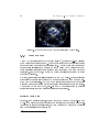
Concept art of the Global Positioning System [3].
3.2
Illustration of Earth and its atmosphere [6].
. . . . . . . . . .
26
3.3
Graphical presentation of dierential GPS [14]. . . . . . . . . .
28
3.4
Microstrain 3DMGX1 IMU [12].
3.5
GlobalSat EM411 GPS receiver with the RS232 interface.
4.1
GPS position aided INS [9].
4.2
4.3
Tightly coupled GPS aided INS [9]. . . . . . . . . . . . . . . .
37
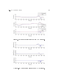
5.1
Stationary position wih GPS dropout.
. . . . . . . . . . . . .
46
5.2
Stationary speed deviation with GPS dropout. . . . . . . . . .
47
5.3
Stationary acceleration deviation with GPS dropout.
. . . . .
47
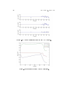
5.4
Dynamic postion estimate with GPS coverage. . . . . . . . . .
49
5.5
Dynamic speed estimate with GPS coverage. . . . . . . . . . .
49
5.6
Dynamic acceleration estimate with GPS coverage.
50
5.7
Bias estimate during dynamic conditions. . . . . . . . . . . . .
50
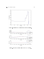
5.8
Measured yaw angle during dynamic conditions. . . . . . . . .
51
5.9
Dynamic postion estimate with GPS dropout.
. . . . . . .
. . . . . . . . . . . . . . . .
24
30
.
31
. . . . . . . . . . . . . . . . . . .
36
GPS range aided INS [9]. . . . . . . . . . . . . . . . . . . . . .
37
. . . . . .
. . . . . . . . .
51
. . . . . . . . . .
52
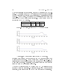
5.11 Position deviation during external inuence, with GPS. . . . .
53
5.12 Speed deviation during external inuence, with GPS.
. . . . .
53
. . . . . . .
54
5.10 Dynamic speed estimate with GPS dropout.
5.13 Acceleration during external inuence, with GPS.
5.14 Position deviation during external inuence, with GPS dropout. 55
5.15 Velocity deviation during external inuence, with GPS dropout. 55
IX
X
LIST OF FIGURES
List of Tables
3.1
WGS-84 ellipsoid properties [15].
3.2
GPS Error Sources, reproduced from [9].
. . . . . . . . . . . .
25
3.3
The NMEA GGA message [2]. . . . . . . . . . . . . . . . . . .
32
3.4
GPS Quality Indicator Values [2]. . . . . . . . . . . . . . . . .
33
3.5
The NMEA RMC message [2]. . . . . . . . . . . . . . . . . . .
33
5.1
RMS values, integrated INS/GPS in static conditions. . . . . .
48
5.2
RMS values, integrated INS/GPS while in motion . . . . . . .
52
5.3
RMS values, integrated INS/GPS with external disturbances .
54
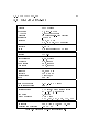
A.1
Microstrain 3DM-GX1 specications [12]. . . . . . . . . . . . .
60
A.2
GlobalSat EM411 specications [5].
61
XI
. . . . . . . . . . . . . . . .
. . . . . . . . . . . . . .
22
XII
LIST OF TABLES
Notation and Abbreviations
Notation
x
R
x
x̂
x̄
x̃
Rba
ẋ
ω aba
Standard typing means that x is a scalar
Boldfaced typing means that
True value of
x
R
is a matrix or vector
x
Measured value of x
Estimated value of
Denotes the error,
x − x̄
R is the rotational matrix that transforms a set of vectors from frame a to frame b
dx
The dot represents time dierentialization of x, ẋ =
dt
Rate of angular rotation of frame a with respect to frame b, coordintized in frame a
Variables
θ
ω
α
p
v
a
Ω
u
v
w
p
q
r
φ
θ
ψ
(Φ, λ)
Euler angles
Rate of angluar rotation
Rate of angular acceleration
Position vector
Velocity vector
Acceleration vector
Skew symmetric form of
ω , Ω = (ω×)
Longitudinal horizontal speed (surge)
Lateral horizontal speed (sway)
Vertical speed (heave)
Body frame roll rate
Body frame pitch rate
Body frame yaw rate
Roll in Euler angle
Pitch in Euler angle
Yaw in Euler angle
Latitude, longitude
XIII
(cross-product)
NOTATION AND ABBREVIATIONS
XIV
Abbreviations
CET
Circular Error Propable
DGPS
Dierential GPS
DoD
(United States) Department of Defense
DOF
Degrees Of Freedom
DoT
(United States) Department of Transportation
ECEF
Earth Centered, Earth Fixed
FAA
(United States) Federal Aviation Administration
GPS
Global Positioning System
IMU
Inertial Measurement Unit
INS
Inertial Navigation System
HDOP
Horizontal Dilution Of Precision
L1
L2
f1
f2
NED
NorthEastDown (frame)
NMEA
National Marine Electronics Association
NTNU
Norwegian University of Science and Technology
RMS
Root Mean Square
SA
Selective Availability
USV
Unmanned Surface Vehicle
UTC
Universal Time, Coordinated
VDOP
Vertical Dilution Of Precision
WAAS
Wide Area Augmentation System
WGS
World Geodetic System
GPS carrier frequency
GPS carrier frequency
Chapter 1
Introduction
1.1
Motivation
Unmanned Surface Vehicles (USV) has been in used in service of the military
since World War II, but has not become largely popular until the 1990s. It is
still commonly found in military applications, but is also increasingly found
in research vessels.
USVs are commonly used to search for underwater mines or underwater activities, investigate the sea bottom, rescue vessels, reconnaissance and surveillance vessels or as a support vehicle for, e.g., an autonomous underwater
vehicles.
Unmanned surface vehicles are usually relatively small, often the size of a
recreational watercraft (below 15 meters), and so far, a USV exceeding 100
tons has yet to be found [1]. As USVs are usually quite small, they are also
somewhat inexpensive compared to larger vessels. Furthermore, as they are
autonomous or remotely operated, proper navigation systems are neccesary
to be able to implement successful control algorithms. As proper navigation
systems usually also has a high price, they are concidered to be unt for
these applications, as they will drastically increase the price of the USV.
1.2
Background
The Global Positioning System (GPS) represents an inexpensive and global
method of obtaining the position of a vessel.
1
Although the measurements
CHAPTER 1. INTRODUCTION
2
are highly subjected to noise, the accuracy can be improved by applying
the principle of dierential GPS. However, the system gives a low bandwith,
especially when it comes to acceleration and speed, which can be calculated
by dierentiating the position measurements.
As a contrast, an Inertial Navigation System (INS) only measures the forces
acting on an Inertial Measurement Unit (IMU), and can thus be used to calculate both speed and position estimates without dierentiating. In addition
to achieving higher bandwiths on the measurements than GPS, this approach
1
gives the estimates the same bandwith as the acceleration measurements .
Furthermore, the INS does not rely on external signals and is therefore not
susceptible to jamming nor the problem of areas lacking satellite coverage.
Using an INS isn't problem free however, as it suers from problems with
drift of speed and position and is also signicantly more expensive than GPS
equipment.
IMUs are placed on a platform inside/on the vessel, referred to as IMU
platform. This will be discussed later in the report.
There are several reasons why an integration of GPS and an INS is desirable.
Generally, an INS gives several advantages that the GPS-system lacks, and
vice versa. Several sources approaches this problem, e.g., [4], [8], [9] and [11].
The main reasons for performing such an integration is:
•
The INS results are available whenever the GPS measurements are unavailable due to, e.g., interference or jamming, and can also be applied
to underwater vehichles
•
The INS measurements are obtained without signicant time delays
•
The INS provides acceleration and speed measurements without dierentiation, and is thus less susceptible to noise
•
Integration provides real time estimates, as opposed to dierentation
•
The GPS corrects the integration error from a stand-alone INS system
•
The GPS allows on-line calibration of IMU errors and alignment of the
IMU platform
1 In other words, by integrating the measurements, position and speed can be obtained
at the same bandwith as the measurement unit.
1.2. BACKGROUND
1.2.1
3
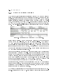
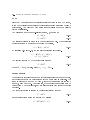
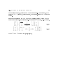
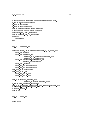
Survey of Existing Solutions
As of this date, several integrated solutions between GPS and INS already
exists, but are in general known to be relatively expensive. For use in low cost
applications, like for a small Unmanned Surface Vehicle (USV), a commercial,
existing integrated solution can easilly exceed the price of the USV itself.
Thus, it is desirable to develop a low-cost integrated solution between a
GPS and an INS, using low-cost components in order to keep the total cost
down.
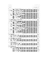
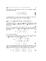
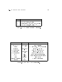
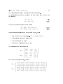
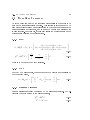
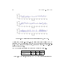
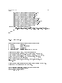
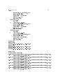
One state-of-the-art integrated navigation system is the Kongsberg
Figure 1.1: Statistics of commercial INS/GPS solutions.
Seatex Seapath series.
As can be seen from Figure 1.1, both the Seapath
100 and 200 is very expensive, but has very little deviation. The Crossbow
1
NAV420CA100 is far cheaper, almost
of the price of the Seapath 200,
10
but in return has a signicantly reduced accuracy. This system is one of the
less expensive products on the marked, but still about 3 times the cost of
the hardware considered for our purposes. Thus a performance close to the
NAV420 will be considered satisfactory.
All the data presented in Figure 1.1 has been obtained from the respective
manufacturers by Maritime Robotics. Most data is presented as Root Mean
Square (RMS) error, with the exceptance of the position accuracy of the
Crossbow solution, which is given in Circular Error Propable (CEP). CEP is
a common measure of the accuracy of weapons, giving the radius of a circle
whence the projectile will land 50% of the time.
Thus the Crossbow will
have a position estimate of less than 3 meters 50% of the time.
Despite all eorts, deviation data for solutions when the GPS is disabled
has not been obtained. This makes it somewhat dicult to come a denite
conclution when comparing two dierent solutions, as this is one of the key
attributes of usch an integrated solution.
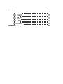
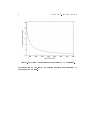
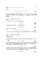
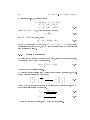
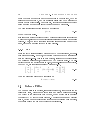
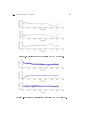
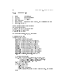
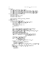
An approximate relationship between performance and price is shown in Figure 1.2, beginning at 40 000 NOK. It is unsure whether this will be accurate
CHAPTER 1. INTRODUCTION
4
Figure 1.2: Accuracy versus price for commercial INS/GPS solutions.
for prices below 60 000, since RMS position deviation for dierential GPS
range as low as 3 meters.
1.3. OUTLINE
1.3
5
Outline
Chapter 1 discusses the motivation for the assignment and shows data for
existing integrated solutions.
Chapter 2 presents dierent reference frames and dierent equations used in
order to transform a vector from one frame to another.
Chapter 3 looks at the history behind the Global Positioning System and
inertial navigation. It also discusses potential errors they are suspectible to
and gives equations for estimating position and speed based on acceleration
measurements.
Chapter 4 outlines the system equations used for integrating the two navigational systems and the approach to estimate attitude, velocity and acceleration.
Chapter 5 shows the results of the integration and compares them with properties from existing solutions
Chapter 6 concludes the report, and also contains a discussion regarding the
concidered product and future work.
6
CHAPTER 1. INTRODUCTION
Chapter 2
Reference Frames and
Transformations
2.1
Reference Frames
In navigation, several reference frames can be used to present the data. Depending on what navigational system is used to obtain the measurements,
dierent reference systems are usually required.
2.1.1
Inertial Frame
For the inertial frame, Newton's law's of motion applies. This means that
the frame itself can not accelerate, but is either stationary or travels with
constant speed. Its origin can be chosen anywhere.
2.1.2
Earth Centered Earth Fixed
The Earth Centered, Earth Fixed (ECEF) frame has, as the name suggests,
its center in the center of the Earth, and the frame is stationary relative to
the surface. Of all the possible combinations of ECEF coordinate systems,
two are of particular importance.
The rst representation frame gives its position in cartesian coordinates,
based on its distance from the center according to each axis. This is named
the ECEF rectangular system but is usually just referred to as the ECEF
7
8
CHAPTER 2. REFERENCE FRAMES AND TRANSFORMATIONS
Figure 2.1: The Earth with both ECEF frames and the local geodetic frame.
◦
system. Its x-axis points through the intersection of the prime median (0
◦
longitude), and equator (0 latitude), its z-axis towards the true north pole,
and the y-axis to complete the right hand rule through the intersection of
◦
90 longitude and equator.
The other representation is called ECEF geodetic frame.
presses position in latitude, longitude and height,
This system ex-
[Φ, λ, h] and is given in the
spherical coordinates. The system takes its basis in the ECEF rectangular
frame. The latitude is found by rotating around the z-axis until the x-axis
crosses the projection from the position on to the x-y-plane. The longitude
is then found by rotating around the y-axis until the x-axis coincides with
the vector from the center of the Earth to the position. The height is the
distance from the nearest point normal on the assumed altitude.
The altitude is assumed to be at the surface of the WGS-84 ellipsoid. WGS84, or the World Geodetic System, is an estimate of Earth dating back to
1984. This ellipsiod will be concidered furter upon developing a gravity model
in Section 3.1.6.
Both ECEF frames are depicted in Figure 2.1, as well as the ENU-frame,
which will be presented later.
2.1. REFERENCE FRAMES
9
Geographic Frame
The geographic frame is dependent on its origin and is only locally correct.
It is earth xed and has its origin at the ellipsoid used to describe the surface
of the Earth. The x-axis points north, the y-axis towards east and the z-axis
points down, normal onto the ellipsoid.
Geosentric Frame
This frame is equal to the geographic frame, with the dierence that its z-axis
is pointing towards the center of the Earth.
2.1.3
Local Geodetic or Tangent Plane
The local geodetic frame is the frame most people consider when orienting
themselves. It takes basis of making a ctional tangent plane at the origin,
just like presenting the globe as a map. The x-axis points north, the y-axis
towards east and the z-axis points down, normal onto the ellipsoid, therefore also widely known as the NED-frame (north-east-down).
This frame
coincides with the geographic frame for a stationary target. The dierence
between the two is that in the latter frame, the origin is a projection of the
platform origin onto the Earth's geoid.
Another version of this frame is the east, north, up-frame (ENU).
2.1.4
Body Frame
In the body frame, the origin is usually in the center of gravity of the body
of the object in question. Its x-axis points towards the dened front of the
object, the z-axis points down and the y-axis points right to complete the
right hand rule. This frame is, together with the NED-frame, widely used
for control purposes.
The frame represents the vessel states in 6 degrees of freedom (6 DOF) known
as surge, sway and heave (u, v, w ), and roll, pitch and yaw (φ, θ, ψ ). Surge,
sway and heave is the speed in x, y and z respectively, and roll, pitch and
yaw is the vehicle's angular displacement from the NED-frame.
10
CHAPTER 2. REFERENCE FRAMES AND TRANSFORMATIONS
2.2
Rotation Matrices and Transformations
In order to transform states from one frame to another, rotation matrices
can be used. For a rotation matrix, subscripted letters indicate the frame it
is being transformed from, while superscripted letters denote the frame the
states are being transformed to. Thus,
Rbp
means the states are transformed from the platform to the body frame.
2.2.1
ECEF Geodetic to ECEF Rectangular
The geodetic coordinates, given in latitude and longitude,
coordinates in two directions, namely north and east.
(Φ, λ)
only gives
The height is then
assumed zero, unless stated otherwise, according to the ellipsoid model of the
Earth's geoid being used. In particular, the WGS-84 ellipsoid is commonly
used.
As already stated, the model parameters will be considered further
when discussing the gravity model in Section 3.1.6, but for now only a few
parameters is of importance.
The ellipsoid has two constants needed to dene the model. These are the
semimajor and semiminor axis, noted as
a and b respectively.
The semimajor
axis is the longest of the two, going horizontally from the center of the Earth,
along the xy-plane in Figure 2.1. The semiminor axis is thus the one pointing
vertically along the z-axis. The length of the semimajor axis is
a = 6378137.0,
while the semiminor axis is only needed to calculate the atness of the ellipsoid, dened as
1
a−b
=
.
a
298.257223563
provided f , an explicit value of b
f=
Since [15] already has
is not needed. Fur-
thermore, the eccentricity of the ellipsoid is dened as
e=
p
f (2 − f ) = 8.1819190842622 · 10−2 .
Finally, the length of the normal of the ellipsoid, from the surface of the
ellipsoid to the intersection with the ECEF z-axis is given as
a
,
N (φ) = p
1 − e2 sin(Φ)2
(2.1)
2.2. ROTATION MATRICES AND TRANSFORMATIONS
11
which is used for the transformation between the two frames. To calculate
rectangular coordinates,
x = (N + h)cos(Φ)cos(λ)
y = (N + h)cos(Φ)sin(λ)
z = [N (1 − e2 ) + h]sin(Φ)
(2.2)
(2.3)
(2.4)
The transformation the other way around is a bit trickier, and is not very
relevant for this report. It will thus not be discussed here.
2.2.2
ECEF-to-Tangent-Plane Transformation
The transformation from ECEF- to tangent-plane coordinates, starts by subtracting the tangent-plane origin, given in the ECEF-frame, from the ECEF
coordinates,
δx = (x, y, z)T − (x0 , y0 , z0 )T ,
leaving the two planes with the same origin.
(2.5)
The next step is performing
a rotation around the ECEF z-axis until the y-axis is aligned with tangentplane east:


cos(λ) sin(λ) 0
R1 =  −sin(λ) cos(λ) 0  ,
0
0
1
where
λ
(2.6)
is the longitude.
By performing a new rotation, this time around the aligned y-axis until the
new z-axis is aligned with the tangent-plane down:

cos(Φ + π2 ) 0 sin(Φ + π2 )

0
1
0
R2 = 
π
π
−sin(Φ + 2 ) 0 cos(Φ + 2 )


−sin(Φ) 0 cos(Φ)
,
0
1
0
=
−cos(Φ) 0 −sin(Φ)

where
φ
(2.7)
is the latitude. Please note that this notation is opposite than that
of [9], as the notation used in this report is believed to be more commonly
used. By combining the two, the complete rotation matrix is obtained,


−sin(Φ)cos(λ) −sin(Φ)sin(λ) cos(Φ)
.
−sin(λ)
cos(λ)
0
RtE = 
−cos(Φ)cos(λ) −cos(Φ)sin(λ) −sin(Φ)
(2.8)
CHAPTER 2. REFERENCE FRAMES AND TRANSFORMATIONS
12
2.2.3
Body-to-Tangent-Plane Transformation
This transformation is performed by using the Euler angles derived from the
body frame and transforming via one axis at a time. By chosing to start with
0 0 0 T
y z
the rotation around the z-axis the new coordinates x
is obtained
 
 
x0
cos(ψ) sin(ψ) 0
x
 y 0  =  −sin(ψ) cos(ψ) 0   y  .
z0
0
0
1
z

(2.9)
The same method is applied to the two remaining axes
 
x00
 y 00  = 
z 00

 
u
 v =
w

 0 
cos(θ) 0 −sin(θ)
x


0
1
0
y0 
sin(θ) 0 cos(θ)
z0
  00 
1
0
0
x


y 00  ,
0 cos(φ) sin(φ)
z 00
0 −sin(φ) cos(φ)
(2.10)
(2.11)
and thus having obtained the body frame coordinates. These can be combined by multiplication, yielding




cos(ψ) sin(ψ) 0
cos(θ) 0 −sin(θ)
1
0
0
  0 cos(φ) sin(φ)  vt
1
0
vb =  −sin(ψ) cos(ψ) 0   0
0
0
1
sin(θ) 0 cos(θ)
0 −sin(φ) cos(φ)
=
cos(ψ)cos(θ)
−sin(ψ)cos(θ) + cos(ψ)sin(θ)sin(φ)
sin(ψ)sin(φ) + cos(ψ)sin(θ)cos(φ)
sin(ψ)cos(θ)
cos(ψ)cos(φ) + sin(ψ)sin(θ)sin(φ)
−cos(ψ)sin(φ) + sin(ψ)sin(θ)cos(φ)
= Rbt vt
2.2.4
−sin(θ)
cos(θ)sin(φ)
cos(θ)cos(φ)
vt
(2.12)
Platform-to-Body Transformation
Assume a rigidly attached point on the vessel where the measurement sensors
are placed. The center of this platform is usually chosen as the origin of the
platform frame.
As the placement of this platform will dier from each
vessel, no standard transformation can be performed.
For inertial sensors
the platform is adviced to be placed near the center of inertia of the vessel
1
while stationary relative to Earth .
1 The center of inertia will shift whenever in motion, particularly for maritime vessels.
2.2. ROTATION MATRICES AND TRANSFORMATIONS
13
First, assume the IMU being placed at the center of inertia, but with angles relative to the body frame noted as
[φr , θr , ψr ].
The rotation to the
body frame is then performed by multiplying with (2.12), substituting the
respective angles with the ones relative to the body frame. Rotation to the
tangent-plane can be performed by adding the body-frame Euler angles to
the relative angles.
Second, should the platform be positioned elsewhere, the rst step is needed
b
to align the axis. Assume r is a vector denoting the correct displacement
from the center, given in body-frame coordinates. As the IMU will detect
accelerations of the given point, regardless of position relative to the object
it is placed on, the position can be calculated as usual, and the position
displacement subtracted from the position,
pb = Rbp pp + rb .
(2.13)
For speed and accelerations, the equation needs to be dierentiated. First,
considering speed,
d b p
[Rp p + rb ]
dt
= Rbp vp + Ṙbp pp
vb = ṗb =
(2.14)
(2.15)
Since the rotation matrix is constant, its derivative is equal to zero.
The
same can be done for the acceleration, yielding
ab = Rbp ap
(2.16)
vb = Rbp vp
(2.17)
14
CHAPTER 2. REFERENCE FRAMES AND TRANSFORMATIONS
Chapter 3
System Consept
3.1
Inertial Measurement Units
As opposed to the GPS, which relies on external synchronization to achieve an
estimate of the position, an Inertial Navigation System measures acceleration
using the physical laws of nature. A pure INS consists only of accelerometers
and gyros, and is based on the principle that estimates of the position and
velocity is obtained by integrating the acceleration.
When reering to Inertial Measurement Units, it is assumed to consist of
a total of three accelerometers and three gyros. Proper IMUs are generally
very expensive, due to need for very accurate measurements. The reason why
accurate measurents are needed, is that the acceleration is integrated twice to
obtain the position. Any error in the acceleration measurement will also be
integrated, and cause a bias on the estimated velocity and a continous drift
on the position estimate, unless corrected. Correcting this error is impossible
on a pure INS', unless recalibrated or reset.
An INS is commonly aided by magnetometers, being able to detect attitude,
and GPS to measure position. For aviation applications, hydroaltimeters are
common to detect altitude. As a single GPS receiver is unable to detect drift
in attitude, it relies on external aiding to correct the error, through, e.g.,
GPS compass
1
or magnetometer.
Originally, INS was developed for missiles, but is today also commonly found
in airplanes, submarines, spacecraft and ships.
1 Two or more GPS receivers placed on two previously known locations, used to estimate
the heading or other Euler angles.
15
CHAPTER 3. SYSTEM CONSEPT
16
3.1.1
Accelerometers
An ideal accelerometer can be viewed as an ideal mass spring damper system,
where the position,
p,
relative to the casing is assumed perfectly measured
[9]. Then
p̈ = −
b
k
p − ṗ,
m
m
(3.1)
where k is the spring constant, b is the damping constant and m is the
mass.
δp
denotes the positional displacement from the equilibrium.
The
force measured from the accelerometers is dened as
f = p̈.
(3.2)
Should the system also be aected by gravity, the equation becomes
p̈ = −
where
g(p)
b
k
p − ṗ + g(p),
m
m
(3.3)
denotes the position-relative gravity. By comparing with (3.1)
and (3.2), it is trivial to see that
f = p̈ − g(p).
(3.4)
In the case of the accelerometers being within the earth's eld of gravity and
rotating around the earth's rate of rotation, i.e., resting on the surface of the
earth, the equation is adjusted into
0=−
where
Ωie
b
k
δp − δ ṗ + g(p) − Ωie Ωie p,
m
m
(3.5)
2
is the skew symmetric form of the earth's rate of rotation vector .
This equation shows that in case of the accelerometer being stationary relative to the earth's surface,
f = −g + Ωie Ωie p.
3
When operating in free fall ,
the accelerometers will read 0. This means that the user needs to compensate
for the forces of gravity when operating an accelerometer.
the local gravity vector,
g, will be dened as -f, or
For the future,
g = g(p) − Ωie Ωie p.
The INS measures the forces in its current position, denoted as
(3.6)
f a , which has
the following properties
f p = Rpa f a ,
2 The equivalent of S(ω i ) or
ie
3 Assuming no rotation.
(ω iie ×)
(3.7)
3.1. INERTIAL MEASUREMENT UNITS
where
17


1
−auw auv
4
1
−avu 
Rpa =  avw
−awv awu
1
(3.8)
auw is to be read as the posiw-axis from the uw-plane to accelerometer
represents the accelerometer displacement where
tive rotation angle about platform
u-axis.
3.1.2
System Equations
The system can be put on rst order form,
ṗ =vn
v̇ =an .
(3.9)
(3.10)
Furthermore, the theorem of Coriolis [9] gives
Ṙba = Rba Ωaba .
(3.11)
Mv̇n = f n − gn = Rnp f p − gn ,
(3.12)
(3.10) can be rewritten as
where
gn
3.1.3
is the gravity vector, and
f is the total force acting on the system.
Velocity Dynamics
Inertial Frame
The dierential equation for the position vector in an inertial frame is given
in (3.4),
p̈ = f + G(p).
(3.13)
As previously stated, this measurementcan be integrated once to obtain inertial speed, and twice for inertial position. The force in a given inertial frame
can be written as a rotation from the body frame,
f i = Rib f b ,
where
Rib
(3.14)
is the rotation matrix from the body frame to the inertial frame.
This can be used to nd the dierential equation for the rotation matrix in
accordance with the theorem of Coriolis stated in (3.11):
Ṙib = Rib Ωbib ,
(3.15)
CHAPTER 3. SYSTEM CONSEPT
18
where
i.e.,
Ωbib


0 −r q
4
0 −p  ,
Ωbib =  r
−q p
0
is the skew symmetric form of
ω bib =4 [p, q, r]T .
This dierential equation is more straight-forward than when using any other
reference frame. However, it is not very commonly used, due to the diculty
in calculating the gravity
G(R).
Inertial Position, Earth-Relative Velocity
This representation of variables is not very commonly used, as they are impractical to work with. However, it is useful as a means to derive the dierential equations of other, more common representations, and is therefore of
importance. Here,
p is dened as the position vector relative to the center
of earth, and for simplicity, the inertial and ECEF orgins are coincident the
center of the earth.
pe = Rei pi .
(3.16)
Furthermore, the dierentiated earth-relative position is the same as the
e
earth-relative speed,
= e . By using the theorem of Coriolis, this rela-
ṗ
v
tionship can be written as
d i
p = vi + Ωiie pi ,
dt
(3.17)
which is dierentiated into
d
d
d2 i
p = vi + Ωiie pi
2
dt
dt
dt
d i
d
d
= v + ( Ωiie )pi + Ωiie pi
dt
dt
dt
d i
= v + Ωiie (vi + Ωiie pi )
dt
d i
d2
v = 2 pi − Ωiie Ωiie pi − Ωiie vi .
dt
dt
(3.18)
d2 i
p represents inertial acceleration, −Ωiie Ωiie pi is the local
dt2
i i
centrifugal acceleration, while Ωie ve denotes the Coriolis acceleration. The
In this equation,
centrifugal acceleration is the same as the gravity, resulting in
d i
v = f i + gi − Ωiie vi ,
dt
where the calculation of
fi
is shown in (3.13) (3.15).
(3.19)
3.1. INERTIAL MEASUREMENT UNITS
19
ECEF
Since the GPS estimates of the position usually are given in the ECEF frame,
it can be convinient to also present the inertial measurements using the same
coordinates.
One drawback with using this conversion is the complicated
gravity calculations.
The position
p and the earth-relative velocity, v, is given as
pe = Rei pi
e
v =
(3.20)
Rei vi .
The relative velocity is given as in the previous example.
(3.21)
The dierential
equation is given by applying the theorem of Coriolis,
v̇e = Rei (v̇i − Ωiie vi ).
(3.22)
By inserting 3.19 into 3.22, the complete expression is obtained.
v̇e = Rei (f i + gi − 2Ωiie vi )
= f e + ge − 2Ωeie ve .
(3.23)
The specic force in ECEF coordinates is given as
f e = Reb f b ,
where
Ṙeb = Reb Ωbeb
is valid, using
(3.24)
ω beb = ω bib − Rbe ω eie .
Local Geodetic
Local geodetic coordinates are the most trivial coordinates for most people,
and corresponds with the coordinates most commonly used in daily life. The
frame is also known as the NED frame, since the coordinates are the same
as north, east and down.
Furthermore, the coordinates are fairly easy to
convert from GPS coordinates, and are also practical with regard to control
purposes.
The geodetic velocity is related to the inertial velocity through
vn = Rni vi .
(3.25)
and is dierentiated using the theorem of Coriolis
v̇n = Rni (Ωini vi + v̇i ).
(3.26)
CHAPTER 3. SYSTEM CONSEPT
20
By inserting (3.19), the result yields
v̇n = Rni (Ωini vi + f i + gi − Ωiie vi )
= f n + gn + (Ωnni − Ωnie )vn
= f n + gn + (Ωne − 2Ωnie )vn ,
where
Ωni = Ωne − Ωie ,
giving the specic force as
f n = Rnb f b ,
and
Ṙnb = Rnb Ωbnb
(3.27)
(3.28)
are valid, using
Ωbnb = Ωbib − Rbn (Ωnie + Ωnen ),
(3.29)
n
is measured by the gyros, ω ie = ω ie [cos(Φ), 0, −sin(Φ)] is the rate
n
of inertial rotation of Earth, and ω en is the transport rate of the navigation
frame relative to earth.
where
ω bib
3.1.4
Position Dynamics
By assuming the velocity vector has been found, like in the previous section,
the position can be found by integrating,
t
Z
v(τ )dτ + p(0),
p(t) =
(3.30)
0
where
p(0) is the initial position.
To obtain geodetic position from tangent plane velocity coordinates, the following dierential equation can be used
 
Φ̇
 λ̇  = 
ḣ

where
Rλ
1
RΦ +h
0
0
0
1
(Rλ +h)cos(λ)
0


0
vN
0   vE  ,
vD
−1
(3.31)
is the radius of curvature in a meridian at a given latitude, and
Rφ
is the transverse radius of curvature,
a(1 − e2 )
RΦ = p
3
1 − e2 sin2 (Φ)
a
Rλ = p
,
1 − e2 sin2 (Φ)
a
being the radius at equator, and
e
being the eccentricity.
(3.32)
(3.33)
3.1. INERTIAL MEASUREMENT UNITS
3.1.5
21
Gyros
The equations obtained in the previous section applies for both strap-down
and stabilized platform systems. The dierence between the two lies in the
stabilized being actuated to maintain its alignment with a given reference
system, while the strap-down system is, as its name suggests, rigidly attached
to the body of the vessel.
Mathematically, the dierence lies in the rotation matrix,
4
Rnp .
The strap-
down system is the easiest to implement , and is also the one being implemented in this report, and is therefore considered. Regardless, both systems
requires information of the rotational vector
ω pnp = ω pip − ω pin .
The gyros experience

ω nin = 
ω pip
and
ω pin = Rpn ω nin .


(3.34)
For tangent-plane navigation,


(λ̇ + ωie )cos(Φ)
cos(P hi)
 = ωie 
+
0
Φ̇

−sin(Φ)
−(λ̇ + ωi e)sin(Φ)
vE
Rλ +h
−vN
RΦ +h
−vE tan(Φ)
Rλ +h



(3.35)
is valid. For obtaining the attitude,
 
 
1 sin(φ)tan(θ) cos(φ)tan(θ)
φ̇
p
 θ̇  =  0
cos(φ)
−sin(φ)   q 
sin(φ)
cos(φ)
0
r
ψ̇
cos(θ)
cos(θ)

(3.36)
can be used.
3.1.6
Gravity Model
For use in a geographic reference system, the gravity is calculated based on
the WGS-84 ellipsoid model [15]. The vector is dened as

 

0
ζg
4
 +  −ηg  ,
0
gn = 
γ(Φ, h)
δg
4 With regard to hardware.
(3.37)
CHAPTER 3. SYSTEM CONSEPT
22
Constant
Value
6378137.0
a
[m]
1
298.257223563
f
e
γa
ω
m
f2
f4
8.1819190842622 · 10−2
9.78049000 [m/s2 ]
7292115.0 · 10−11 [rad/s]
0.00344978650684
−f + 25 m + 12 f 2 − 26
f m + 15
m2
7
4
− 12 + 52 f m
Table 3.1: WGS-84 ellipsoid properties [15].
with
1
2
γ(Φ) = γa 1 + (f2 + f4 )sin (λ) − f4 sin (2Φ)
(3.38)
4
2γh
5
3γa
2
γ(Φ, h) = γ(Φ) −
1 + f + m + (−3f + m)sin (Φ) h + 2 h2 .
2
2
a
2
(3.39)
The parameter values for the gravity model are given in Table 3.1.
For
maritime applications, (3.39) is not considered, since the height is close to
constant at
h = 0.
3.2. GLOBAL POSITIONING SYSTEM
3.2
23
Global Positioning System
When talking about the Global Positioning System (GPS), people usually
refer to the NAVSTAR GPS, which was originally developed by the United
States Department of Defense for use in military applications [13].
In 1983, a Korean airliner was shot down by the Soviet air force. Since the
disaster could have been avoided with access to a proper navigation system,
Ronald Reagan decided to open the NAVSTAR project for the public. GPS
has since then become very popular due to its low cost, availability and
accuracy.
Russia also has a similar global positioning system, called the GLONASS, and
the European Union's Galileo is to be completed around 2011. In addition,
China's regional satellite system, Beidou, has been proposed extended to
a global system called COMPASS. Some GPS receivers make use of both
GLONASS and NAVSTAR data to increase accuracy.
GPS can be divided into space, control and user segments [9]:
•
The space segment is the satellites orbiting the earth.
It consists of
six planes with four satellites on each plane for a total of 24 satellites.
These planes are arranged in such a way that gives at least six satellites
line of sight to almost any given point at all times.
•
The control segment monitors the health and status of the satellites. It
consists of six monitoring stations located in Cape Canaveral, Ascension Island, Kwajalein, Diego Garcia, Hawaii, and Colorado Springs.
The four rst also have each its ground antenna. These stations send
clock corrections and orbital model to the satellites via the antennas.
•
The user segment is the GPS reciever.
In order to work, it needs
an antenna tuned in to the frequencies used by the satellites.
The
reciever also has a high accuracy clock, usually being driven by a quarts
oscillator.
The GPS transmits data signal over two main carrier frequencies, called L1
and L2, transmitting on 1575.42 and 1227.60 MHz respectively. All data is
trasmitted using the Coarse/Acquisition (C/A) code, which is available to
the public, and the Precise (P) code used by the military. L1 transmits both
the C/A and the P code, while L2 transmits the P code. Both frequencies
are available for all users, but due to encryption of the P code, only the C/A
is usable by the public.
CHAPTER 3. SYSTEM CONSEPT
24
Figure 3.1: Concept art of the Global Positioning System [3].
3.2.1
Error Sources
5
1
ms will lead
1000
to a measurement error of 300 m. Thus the timing needs to be highly accurate
As the GPS signals travel with the speed of light , an error of
in order to give an acceptable measurement. The time bias can be assumed
equal for all satellites and accounted for by using the measurement from
three satellites simultaneously (solving four equations with four unknown
variables). In other words, a minimum of four satellites are needed in order
to achieve position.
However, several factors still contribute to the GPS error. It is appropriate
to separate the error sources into two main groups; common mode and noncommon mode errors [9]. Common mode errors are errors that occur within
a limited geographic region and are equal for all recievers within the region.
As opposed to common mode, non-common mode errors refer to reciever
individual errors that can occur independent of location.
Receiver Clock Bias
Table 3.2 shows a list of errors, divided into common mode and non-common
mode. One error that is not included in this list is the receiver clock bias.
This error is equal for all signals, and can therefore be estimated if signals
from four satellites are available by:
5 Approximately
3 · 108 m/s
3.2. GLOBAL POSITIONING SYSTEM
Errors
Common Mode
25
Standard Deviation
Selective Availability
Ionosphere
Clock and ephemeris
Troposphere
Noncommon Mode
24.0
7.0
63.6
0.7
Reciever Noise
0.1-0.7
Multipath
0.1-3.0
Table 3.2: GPS Error Sources, reproduced from [9].
1. Dierentiating two simoultaneous measurements from the same receiver
2. Calculating an estimate at each time step
3. Estimating the error as a state using a dynamic model and Kalman
ltering
Although not in Table 3.2, this error is receiver individual, and can be viewed
as non-common mode.
Atmospheric Eects
One problem with calculating the distance from the satellite based on the
time a signal uses on its journey from the satellite to the receiver is that the
signal has dierent speed based on the substance it travels through.
This
also applies for the Earth's atmosphere, and particularly the ionosphere.
6
However, as the speed of signals in this layer is dependent on frequency , a
two-frequency receiver can estimate this error easily. For a single-frequency
receiver, the estimate is dependent on atmospheric modelling.
The dierent layers of the atmosphere can be viewed in Figure 3.2
The ionosphere is the upmost part of the atmosphere, and is ionized by solar
radiation.
From the display given in Figure 3.2, it is located within the
Thermosphere.
As atmospheric errors are dependent on the distance the signal travels through
the atmosphere, they are smallest when the satellite is positioned straight
6 This phenomenon is also known as dispersion
CHAPTER 3. SYSTEM CONSEPT
26
above the receiver.
The more correct the estimated position is, the more
accurately the atmospheric error can be calculated.
Another atmospheric error is the tropospheric delay, which is dependent on
atmospheric pressure, temperature, humidity and satellite elevation.
This
delay is usually separated into a wet and a dry component, where the dry
component contributes to approximately 90 % of the delay. This component
is relatively well modelled, while the wet one is more complicated due to
many local factors. There are several dierent models for the tropospheric
delay, which are good or bad depending on the angle of the satellite.
As
opposed to the ionospheric error, the tropospheric delay is not frequency
dependent and more locally varying, making it dicult to estimate.
Figure 3.2: Illustration of Earth and its atmosphere [6].
Selective Availability
Selective Availability (SA) is an articial feature designed by the U.S. Department of Defense.
Its purpose is to introduce slowly changing random
errors to avoid the GPS being used for military purposes (by other than the
U.S.) or terrorist activites. However, this feature is currently disabled (since
2000), and will therefore not be discussed further.
Multipath
Multipath errors are a result of signals reected o surfaces on the way to or
in the vincinity of the receiver, causing the signal to travel further than the
3.2. GLOBAL POSITIONING SYSTEM
27
direct path, thus causing it to use a longer time to the receiver or the same
signal to arrive twice. C/A multipath errors are usually from 0.1 - 3 m, but
errors up to 100 m have been reported.
For L1 carrier phase, the error is
assumed to be less than 5 cm.
Should a signal arrive either twice after a newer signal due to multipath,
the old signal will simply be neglected.
However, if the signal simply is
delayed and no other signals arrive at the receiver in the mean time, it is
nearly impossible to separate the error from other errors.
However, some
precautions can be made:
•
Using an antenna with low gain at low and negative elevations, due to
most reecting surfaces being below the receiver
•
If possible, place the receiver higher than the highest reector
•
Do not accept signals from satellites at low elevation, as these travel
nearly parallell to the surface and are thus more error-prone to reections
Avoiding multipath is extremely important when choosing sites for DGPS
reference stations, as multipath errors are non-common mode errors, and
will manifest themselves in the error estimate sent from the station.
Receiver Noise
The receiver noise is assumed to be white, and is a result of error in measuring
transit time.
The error is due to factors such as nonlinearity and thermal
noise. It is highly dependent on hardware selection in the receiver, and will
therefore vary with the quality of the GPS receiver.
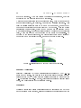
3.2.2
Dierential GPS
As seen from Table 3.2, the most signicant contribution to the error on
the estimated position comes from the common-mode errors. By setting up
a stationary reciever at a known position, the readings will be aected by
the same common-mode errors as any other reciever in the area. Since the
position is already known, the error can be calculated by subtracting the
measurement from the receiver by the known position.
This error can be
broadcasted together with the corresponding clock readings.
Thus, every
CHAPTER 3. SYSTEM CONSEPT
28
receiver in the vicinity can obtain the error and adjust for it.
The error
calculated by the reference station will be assumed to be the common-mode
error and is subtracted from the measurement.
The disadvantage of using DGPS is the lack of global coverage.
Figure 3.3: Graphical presentation of dierential GPS [14].
The United Stated Federal Aviation Administration (FAA) and the United
States Department of Transportation (DoT) has constucted a feature called
the Wide Area Augmentation System (WAAS) [7]. Described shortly, WAAS
is similar to the DGPS system, but only accessible in North-America and is
mainly designed for aerial applications. WAAS is not certied for maritime
navigation, and it is claimed that DGPS has a higher accuracy whenever
close to the reference station. Due to WAAS being unavailable outside NorthAmerica, and the fact that it has not yet been certied for marine applications
[7], it will not be discussed further.
3.2.3
Velocity Measurements
Navigational charts and other tools such as GPS measurements are usually
given in an ECEF geodetic reference frame, using latitude, longitude and
altitude, denoted as
[Φ, λ, h] respectively.
For presentation or using as aid to
an INS, both ECEF and a local geodetic frame can be used. The local geodic
frame is usually preferred whenever operating within a small area. For larger
areas of operation, ECEF is concidered inertial.
There are several ways to perform the integration between GPS and INS,
depending on the frame desired. In this report, integration is performed in
3.2. GLOBAL POSITIONING SYSTEM
two dierent frames, depending on the measurement.
geodetic
29
For position, ECEF
(Φ, λ, h) is used, while for speed, the tangent-plane (NED) has been
chosen.
In order to transform the GPS data, the position, already given in ECEF
geodetic coordinates, is dierentiated. To transform the speed, (3.31) is used,


  1
0
0
Φ̇
vN
RΦ +h
1
 λ̇  =  0
0   vE 
(Rλ +h)cos(Φ)
vD
ḣ
0
0
−1

 


Φ̇
vN
RΦ + h
0
0
 vE  = 
0
(Rλ + h)cos(Φ) 0   λ̇  ,
vD
0
0
−1
ḣ

where
RΦ
and
Rλ
is given in (3.32)(3.33).
(3.40)
(3.41)
CHAPTER 3. SYSTEM CONSEPT
30
3.3
Hardware Selection
As this report will consider the implementation of an integrated navigation
system, hardware is needed. The IMU has been chosen mainly according to
price, while the GPS module has been recycled from an earlier Unmanned
Aerial Vehicle (UAV) project at NTNU [8].
3.3.1
IMU
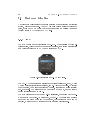
The IMU chosen is the Microstrain 3DMGX1.
This consists of three ac-
celerometers, three gyros and three magnetometers, thus giving acceleration
in 6 degrees of freedom (6 DOF) and position in 3 DOF.
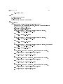
Figure 3.4: Microstrain 3DMGX1 IMU [12].
The 3DNGX1 guarantees an accelerometer bias stability of 0.010 G, where
◦
G is the Earth's gravitational constant, and 0.7 /sec for the gyros. To correct
the gyro error, the magnetometers can be used, operating at a bias stability
of 0.010 gauss.
The sensors have a bandwidth of 100 Hz, and are able to
detect accelerations up to 500 G.
The IMU transmits data over an RS232 serial line, depending on the command sent to the device. As a standard, the 3DNGX1 transmits a message
each time the given command byte is sent, but continuous mode can be
enabled, making the IMU transmit a given message continuously.
3.3. HARDWARE SELECTION
3.3.2
31
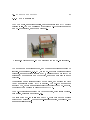
GPS Receiver
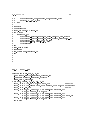
The GPS module, as mentioned earlier, has been recycled from a UAV project
detailed in [8]. The GPS consists of a GlobalSat EM411 receiver mounted
on a RS232 interface, as shown in Figure 3.5.
Figure 3.5: GlobalSat EM411 GPS receiver with the RS232 interface.
The module has no internal power, and thus needs external powering to
function. It operates at 4.5 6.5 V, but the RS232 board contains a voltage
converter, making it able to operate at 9 V, meaning it can be powered by an
external 9 V power supply or a PP3 battery, most commonly used in smoke
detectors.
This receiver has a position accuracy of 10 meters, or 5 meters with Wide
Area Augmentation System (WAAS) enabled.
The EM411 module does
support DGPS, but its manual does not list the accuracy for DGPS. However,
the accuracy can be assumed close to that of WAAS.
The EM-411 receiver supportes NMEA 0183 protocol, which is also the standard setting, discussed in Section 3.3.3.
The price of the EM411 is less than 500 NOK. More data on the module is
provided in Appendix A. For hardware-interested readers, the full EM411
manual is available at [5].
CHAPTER 3. SYSTEM CONSEPT
32
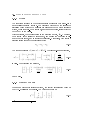
3.3.3
NMEA 0183
The NMEA 0183 is a standard developed by the National Marine Electronics
Association and uses ASCII communication over the serial line. The standard
is commonly used in marine measurement devices like GPS receivers. The
message header can be divided in three parts; rst, a $-sign implying the
start of a message followed by a prex containing a device identier specied
by the protocol.
The nal three letters contain the type of message being
sent, however only two are particularly relevant for obtaining the position,
hence GGA and RMC. Only these two will be explained in the following text.
More information can be found in [2].
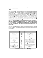
The GGA sux denotes the Global Positioning System Fix Data. It contains time, position and x related data for a GPS receiver. Table 3.3 shows
a GGA message with a description of each message part. For messages using
the NMEA 0183 standard, each part of the message are separated with the
',' delimiter.
The RMC sux indicates the contents of the message being the Recommended Minimum Navigation Information. An example message is shown
in Table 3.5.
Name
Example
Description
Message ID
$GPGGA
Message header
Time (UTC)
123456.123
[hhmmss.sss]
Latitude
6325.0840
[ddmm.mmmm]
N/S Indicator
N
North (N) or South (S)
Longitude
01024.1304
[dddmm.mmmm]
E/W Indicator
E
East (E) or West (W)
GPS Quality Indicator
1
See Table 3.4
Number of satellites
09
00 - 12
HDOP
2.1
Horizontal dilution of precision
Altitude
56.1
Altitude relative to geoid
Units
M
Units of antenna altitude
Geoidal separation
10.1
WGS-84 height deviation
Units
M
Units of geoidal separation
Age of di. GPS data
Null eld without DGPS
Di. ref. station ID
0000
Checksum
*6B
0000-1023
Table 3.3: The NMEA GGA message [2].
3.3. HARDWARE SELECTION
Value
33
Description
0
Fix not available or invalid
1
GPS SPS Mode, x valid
2
Dierential GPS, SPS mode, x valid
3
GPS PPS Mode, x valid
Table 3.4: GPS Quality Indicator Values [2].
Name
Example
Description
Message ID
$GPRMC
Message header
Time (UTC)
123456.123
[hhmmss.sss]
Status
A
A = data valid, V = data invalid
Latitude
6325.0840
[ddmm.mmmm]
N/S Indicator
N
North (N) or South (S)
Longitude
01024.1304
[dddmm.mmmm]
E/W Indicator
E
East (E) or West (W)
SOG
0.16
Speed over ground [knots]
COG
46.98
North relative to north [deg]
Date
220508
[ddmmyy]
Magnetic variation
E
East or West [deg]
Checksum
*6B
Table 3.5: The NMEA RMC message [2].
34
CHAPTER 3. SYSTEM CONSEPT
Chapter 4
Integrating GPS and INS
4.1
Approaches
There are several ways to implement a GPS/INS integration. First of all, we
dier between the direct-ltering and the complementary-ltering approach
[9].
4.1.1
Direct-Filtering
Direct-ltering is perhaps the most intuitive of the two.
It uses position
and velocity as states in a state space representation, with GPS data as
measurements (y) and the inertial measurements as input (u) in a Kalman
lter. While this seems straight forward, it has three major drawbacks:
1. The Kalman lter covariance equations have to be calulated at the rate
of the inertial measurements. As these equations require much CPU,
the bandwith of the inertial measurements are highly restricted
2. The measurements have highly deterministic components that will be
represented by ad hoc models in the state space representation.
3. The states can change dramatically between iterations, which require
high lter bandwith.
Complementary-ltering considers the inertial measurements and mechanization equations as two separate systems, giving the Kalman lter a reference
35
CHAPTER 4. INTEGRATING GPS AND INS
36
trajectory.
When new GPS measurements arrive, the INS states are com-
pared to the GPS data. By running the dierence between the two sets of
data through a second Kalman lter, a set of error equations can be estimated.
This implementation enables the covariance update equations to be calculated only at each GPS measurement, reducing the total computational load.
4.1.2
Complementary-Filtering
For the complementary-ltering approach, there are three dierent solutions,
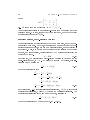
loosely coupled GPS position and range aided INS, plus a tightly coupled
approach.
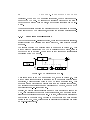
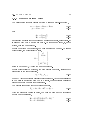
The loosely coupled GPS position aided INS is shown in Figure 4.1.
This
method uses the position from the GPS to calculate the INS error, which is
fed back to the INS system. This method is very simple and requires little
processing of the GPS output.
Figure 4.1: GPS position aided INS [9].
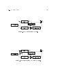
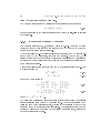
A similar method is the GPS range aided INS, shown in Figure 4.2.
This
method uses a range predictor to transform the INS measurements to a range
prediction, while comparing these to the GPS range measurements.
This
approach gives a better system performance than the position aided system,
but requires the understanding and processing of GPS data, which may be
unavailable for o-the-shelf hardware.
Finally, the tightly coupled solution uses INS data as feedback also to the
GPS. This decreases the bandwith of the tracking loop, and makes the system
less prone to interference and jamming. However, this approach requires not
only access to the range data, but also to the hardware and Kalman lter
design in the GPS. Thus, this approach is generally not available when using
an o-the-shelf receiver.
4.1. APPROACHES
Figure 4.2: GPS range aided INS [9].
Figure 4.3: Tightly coupled GPS aided INS [9].
37
CHAPTER 4. INTEGRATING GPS AND INS
38
4.2
GPS Position Aided INS
The GPS position aided INS is dened as an INS using the GPS position to
adjust for the drifting due to INS acceleration error [9]. It is useful to put
the system equations on state space form
ẋ = Ax + Bu + f (x, u) + Dν
y = Cx + w,
where
x
is the states,
dierential equation,
u
ν
is the input,
f(x,u)
Combining (3.27) with (4.1), using
x=
(4.2)
is the non linear parts of the
is the process noise and
(4.1)
p v
w is the measurement noise.
T
, the system can be written
as
t
ẋ =
where
bp
0 I
0 0
t
x +
0
t p
Rp (f̄ + bp ) − gt
+
0
t
(Ωet − 2Ωtie )vt
(4.3)
is the accelerometer bias, calculated in the Kalman lter and


(Φ̇ + 2ωie )cos(λ)

ω tet + 2ω tie = 
−λ̇
−(Φ̇ + 2ωie )sin(λ)
0 is used throughout this document, meaning I3×3 and 03×3
1
otherwise . The input, u, is the measured force from the INS,
For simplicity,
unless stated
I
(4.4)
and
f̄ = f + f̃ .
For a simpler transition between GPS and INS states, (4.3) can be rewritten
to give its position in ECEF geodetic coordinates (Φ, λ, h).
Eg
achieved using Rt
given in (3.31), yielding
This is easilly
E
0
0
0 Rt g
ẋ =
x+
+
Rnp (f̄ p − bp ) − gn
(Ωtet − 2Ωtie )vt
0 0
y = I 0 x + w,
n
(4.5)
(4.6)
Combining these equations, the resulting equations yields


−(Φ̇ + 2ωie )sin(λ)vE + λ̇vD
v̇t =f̄ t − bt + gt +  (Φ̇ + 2ωie )sin(λ)vN + (Φ̇ + 2ωie )cos(λ)vD 
−(Φ̇ + 2ωie )cos(λ)vE + λ̇vN
 1

0
0
Rλ +h
E
1
0  vt
ṗEg = Rt g vt =  0
(RΦ +h)cos(λ)
0
0
−1
1 This applies only for the boldfaced notation.
(4.7)
(4.8)
4.2. GPS POSITION AIDED INS
39
The bias calculation will be discussed later in this chapter.
The relationship between the measured and true output from the INS can
be written as
f̄ p = f p + f̃ p
ω̄ pnp = ω pnp + ω̃ pnp ,
(4.9)
(4.10)
where the the error equation is given as [9]
f̃ p = Ãa f p + δba + δnla + ν a
ω̃ pip = δAg ω gip + δbg + δnlg + ν g .
(4.11)
(4.12)
These equations are also known as the truth model, where
• δb
is a random walk variable, e.g.
• δnl
• ν
δ ḃ = ν b
where
Pb (ν) = 0
represents all the non linear errors
is the measurement noise
• δA
is due to misalignment of the IMU
The misalignment matrix is given as

δSFu −δauw

δavw
δSFv
δAa =
−δawv δawu

δSFp −δapr

δaqr δSFq
δAg =
−δarq δarp
and
δnl

δauv
−δavu 
δSFw

δapq
−δaqp  ,
δSFr
is the nonlinear error, given as

kx1 fu2 + kx2 fv2 + kx3 fw2 + kx4 fu fv + kx5 fv fw + kx6 fw fx
δnla =  ky1 fu2 + ky2 fv2 + ky3 fw2 + ky4 fu fv + ky5 fv fw + ky6 fw fx 
kz1 fu2 + kz2 fv2 + kz3 fw2 + kz4 fu fv + kz5 fv fw + kz6 fw fx


kp1 fp2 + kp2 fq2 + kp3 fr2 + kp4 fu fv + kp5 fv fw + kp6 fw fu
δnlg =  kq1 fp2 + kq2 fq2 + kq3 fr2 + kq4 fu fv + kq5 fv fw + kq6 fw fu  .
kr1 fp2 + kr2 fq2 + kr3 fr2 + kr4 fu fv + kr5 fv fw + kr6 fw fu

CHAPTER 4. INTEGRATING GPS AND INS
40
Since the truth model gives a lot of parameters to be estimated, both the
alingment error matrix
A, and the nonlinear errors tend to be neglected to
ensure proper observability.
Furthermore, acceptable results are achieved
using an error model of only slowly varying bias and white noise.
The bias dierential equation should be modelled as
ṗ = ν,
where
ν
(4.13)
is white noise.
It is also worth noting that since the IMU chosen in this experiment includes a
magnetometer, leading to the unit internally calculating position and angular
velocity. Thus, the above equations regarding angular motion has not been
used, as the IMU angular output was used directly.
4.2.1
GPS
Since the IMU position is already given in the ECEF geodetic frame, no transformation is required. However, the velocity vector needs to be transformed
into the tangent-plane. This is an easy process, starting with dierentiating
two position measurements, obtaining the ECEF geodetic speed. By multiplying this with the matrix gained in (3.31), tangent-plane speed is achieved,
For the GPS, its equations are already given in (3.41),

 


Φ̇
vN
RΦ + h
0
0
 vE  = 
0
(Rλ + h)cos(Φ) 0   λ̇  .
vD
0
0
−1
ḣ
(4.14)
Thus the esimation error can be calculated as
x̃ = xGP S − xIM U
4.3
(4.15)
Kalman Filter
The Kalman lter is an optimal, linear state estimator, able to estimate the
full system state, depending on incomplete and noisy measurement series.
The theory of the lter dates back to 1960, when Rudolf Kalman proposed
the lter to NASA for the Apollo Program. The lter comes in many dierent
forms, but the one most relevant for this work is the discrete Kalman Filter,
which also will be the one most thoroughly investigated.
4.3. KALMAN FILTER
4.3.1
41
Discrete Kalman Filter
The dicrete lter takes its basis in a system written on state-space form,
xk+1 = Ak xk + Bk uk + Dk ω k
yk = Ck xk + ν k
(4.16)
Qk = E[ω k ω Tk ]
(4.18)
(4.17)
with
Rk =
E[ν k ν Tk ]
(4.19)
as covariant matrices for the process and measurement noise, respectively. It
is assumed that both
Q and R are known.
As there are no input,
u, in the
system, this can be neglected.
Should the system be observable, the Kalman lter can be used. To ensure
observability, the observability matrix,




O=



needs to have rank
n, n
C
Ck Ak
·
·
·
n−1
Ak Ck




,



(4.20)
being the number of states.
Should observability be obtained, the ter process can begin, starting with
estimation of the state variables,
x−
k = Ak−1 xk−1 ,
where
xk−1 is the previously calculated state estimate.
(4.21)
As the bias calculated
in the lter is subtracted from the INS states, this previously calculated
estimate needs to be reset every interation.
The process is repeated for the covariance matrix,
T
P−
k = Ak−1 Pk−1 Ak−1 + Qk−1 .
(4.22)
With the estimated values in place, the Kalman gain and the covariance
update can be calculated,
− T
T
−1
Kk = P−
k Ck [Ck Pk Ck + Rk ]
Pk = I − Kk Ck P−
k,
(4.23)
(4.24)
CHAPTER 4. INTEGRATING GPS AND INS
42
using the previously calculated estimates.
The Kalman gain are used to calculate the nal estimate of the states
xk = Kk [yk − Ck x−
k]
(4.25)
Proper derivation of the lter equations can be found in [9], [10] or several
other sources.
4.3.2
Integration Kalman Equations
The Kalman lter input,
y,
is already given in (4.15).
This can be used
together with the knowledge of the error of the GPS and the INS data to
derive the state space error equations.
As the Globalsat EM411 fails to deliver sudo ranges, the GPS error is assumed only to be white noise, although not correct.
For the IMU, it is
already stated that the bias should be estimated as integrated white noise in
addition to a white noise component directly on the signal to correspond to
the measurement noise.
Using these assumptions together with the INS equations derived in 4.5, the
model takes form as
g t
˜ Eg = RE
ṗ
t v
(4.26)
t
˜ = −bt + ν ta ,
v̇
(4.27)
which can be rewritten as



E
0 0
0 Rt g 0
ẋ =  0 0 −I  x +  I 0  ν
0 I
0 0
0
I 0 0
I 0
y=
x+
w,
0 I 0
0 I
T
ṽt bt .

where
x=
p̃Eg
(4.28)
(4.29)
The estimated position and speed error are then subtracted from the original
states calculated from the IMU measurements.
As the bias is likely to be
following each of the accelerometers, it needs to be transformed back to the
platform frame immediatetly after calculated. This transformation is to be
performed using the mean value of the attitude measurements, dating back
to the previous lter update.
4.4. EQUATIONS SUMMARY
4.4
43
Equations Summary
To give a quick summary of the equations given earlier in the report to be
used in the actual integration process.
This section is reccomended to be
read after having obtained an understanding of what has been written in the
previous sections of this report, and is meant to be used as a reference for
implementation. Furthermore, it will only assess the equations used in the
actual implementation of the total system.
4.4.1
IMU


−(Φ̇ + 2ωie )sin(λ)vE + λ̇vD
v̇t =Rtp (f̄ p + bp ) + gt +  (Φ̇ + 2ωie )sin(λ)vN + (Φ̇ + 2ωie )cos(λ)vD 
−(Φ̇ + 2ωie )cos(λ)vE + λ̇vN
(4.30)

ṗ
Eg
=
E
Rt g v t
=
1
Rλ +h
0
0
0
1
(RΦ +h)cos(λ)
0

0
0  vt
−1
(4.31)
which is to be computed at each iteration.
4.4.2
GPS
For the GPS measurements, the speed needs to be derived and transformed
to the tangent plane,

vt = RtEg vEg
4.4.3

Rλ + h
0
0
0
(RΦ + h)cos(λ) 0  vEg .
=
0
0
−1
(4.32)
Kalman Filtering
Kalman ltering is applied whenever a GPS measurement arrives. The ltering is done with regard to the error equations,
g t
˜ Eg = RE
ṗ
t v
˜ t = −bt + ν na ,
v̇
(4.33)
(4.34)
CHAPTER 4. INTEGRATING GPS AND INS
44
which can be written on state space form



E
0 0
0 Rt g 0
ẋ =  0 0 −I  x +  I 0  ν
0 I
0 0
0
I 0 0
I 0
y=
x+
w
0 I 0
0 I

using
x=
p̃Eg ṽt bt
T
(4.35)
(4.36)
.
These equations are put on discrete form and fed into the Kalman lter
equations, given in (4.20)(4.25),
x−
k = Ak−1 xk−1
(4.37)
P−
k
(4.38)
=
Kk =
Pk =
xk =
Ak−1 Pk−1 ATk−1 + Qk−1
− T
T
−1
P−
k Ck [Ck Pk Ck + Rk ]
I − Kk Ck P−
k
Kk [yk − Ck x−
k ].
(4.39)
(4.40)
(4.41)
Furthermore, as the bias is subtracted from the respective states, the estimated bias needs to be set zero every iteration.
Chapter 5
Results
All simulations and tests have been performed in Matlab, using Runge-Kutta
4 for solving the dierential equations. A c++ implementation has also been
made for real time implementation, based on the existing code at Maritime
Robotics, but this code had performance issues due to only using an old
laptop with insucient computation capabilities.
Also, due to this thesis being somewhat delayed, all results have been obtained during the summer vacation, meaning that any tests on a boat was
hard to perform. Thus, all tests have been made within a small area, while
attempting to simulate a USV-like environment.
At the Microstrain IMU, the z-axis is pointing upwards (despite the drawing
on the IMU, telling it points down), meaning that the z-axis needs to be
inverted. The other axis are correct as they are marked on the IMU, completing the right hand rule. Also the yaw angle seems to be measured against
◦
west instead of north, meaning 90 has to be subtracted from the yaw angle.
Both the z-axis correction and the yaw angle correction are contrary to what
stands in the manual, and it is unknown whether this is a manufacturing
error.
Covarianse matrices has been found by sampling GPS and IMU measurements, and calculating the covariance oine.
All test results shown are taken from several samples in an attempt to capture
the worst-case results. This is due to some of the tests results being result of
pure luck, leading to a better performance then what can really be expected.
45
CHAPTER 5. RESULTS
46
5.1
Stationary Tests
Figure 5.1: Stationary position wih GPS dropout.
For preliminary tests, both the IMU and the GPS receiver were kept stationary and the measurements were logged in Matlab. By using these measurements as input into the model found in the previous chapter, the equations
were tested to determine any errors. At 40 to 60 seconds, the GPS disconnects.
This process were not done in real-time, solving another problem, hence the
lack of proper computational hardware.
As can be seen from Figure 5.3 the acceleration estimates manage to converge
towards 0, resulting in a maximum deviation of less than 10 meters after 40
seconds without GPS-aid in the east direction, the result shown in Figure
5.1.
Although these gures shows promising results, they should not be taken
into to high regard however, as the system is stationary. However, they do
show that the simplications of the IMU equations is close to that of the
truth model, and that the system performs satisfactory so far, as long as the
GPS measurements are credible.
5.1. STATIONARY TESTS
Figure 5.2: Stationary speed deviation with GPS dropout.
Figure 5.3: Stationary acceleration deviation with GPS dropout.
47
CHAPTER 5. RESULTS
48
Table 5.1 shows the root mean square values of the deviation in acceleration,
speed and position with the GPS being online.
North/East
Down
Acceleration (RMS)
0.05
0.02
Velocity (RMS)
0.09
0.01
Position (RMS)
3
0.005
Table 5.1: RMS values, integrated INS/GPS in static conditions.
Calculating RMS values during GPS dropout would be pointless, as this will
increase exponentially over time.
Comparing Table 5.1 with Figure 1.1, it is clear to see that the low cost
application range within the specications of the Crossbow NAV420, and
is about twice to that of the Kongsberg Seatex Seapath 100 while being
stationary, meaning that the success of the low cost application is feasible. It
is worth noting however, that the down-component has such low Root Mean
Square readings due to the altitude of the USV being assumed 0 whenever
GPS measurements arrive.
5.2
Dynamic Tests
Next, it's time to test the system in motion.
As no proper system were
availiable for benchmarking, a previously known path were set up in order
to test the performance.
After approximately 40 seconds, the IMU is assumed to be proper calibrated,
and is moved in a square-like path of about 5×5 meters, always moving in
the direction of IMU's x-axes. During the rst run, the GPS is constantly
online. The results is shown in Figures 5.4 5.6.
As can be seen from Figure 5.4, the position deviation is not that large. The
measurements from the GPS are a bit to low according to the real path,
whereas the true position lies somewhere in between the two.
Regardless,
the Kalman lter corrects the INS estimates quite conciderably, which can
easily be seen from the speed estimates in Figure 5.5.
The estimated bias is shown in Figure 5.7
It may also be worth taking a look at Figure 5.8, showing the yaw angle
measurement, which is quite accurate.
5.2. DYNAMIC TESTS
Figure 5.4: Dynamic postion estimate with GPS coverage.
Figure 5.5: Dynamic speed estimate with GPS coverage.
49
50
CHAPTER 5. RESULTS
Figure 5.6: Dynamic acceleration estimate with GPS coverage.
Figure 5.7: Bias estimate during dynamic conditions.
5.2. DYNAMIC TESTS
Figure 5.8: Measured yaw angle during dynamic conditions.
Figure 5.9: Dynamic postion estimate with GPS dropout.
51
CHAPTER 5. RESULTS
52
Due to uncertainties on true position, it is hard to calculate the RMS correctly. By wrongfully using the GPS measurements as the correct position,
the RMS values for the deviation can be calculated. The results are shown in
Table 5.2. As can be seen, the position RMS is actually lower in north/east
direction than it was during static conditions.
This is merely due to the
subtraction of the GPS position.
North
East
Down
Velocity (RMS)
2.0428
1.4548
0.6307
Position (RMS)
2.1724
1.3248
0.3350
Table 5.2: RMS values, integrated INS/GPS while in motion
Figure 5.10: Dynamic speed estimate with GPS dropout.
It is also worth noting what happens when the GPS is oine during when
moving through the course. As can be seen from Figures 5.9 and 5.10, the
results are somewhat positive despite a high magnitude on the position, and
a high drift downwards. Regardless, the deviation north and down are very
large compared to what is really acceptable.
As the IMU is also supposed to be placed on a USV, it will also become
subject to waves and vibrations. To simulate this, the IMU was kept nearly
stationary, while being rotated and moved back and forth in small circles.
5.2. DYNAMIC TESTS
Figure 5.11: Position deviation during external inuence, with GPS.
Figure 5.12: Speed deviation during external inuence, with GPS.
53
CHAPTER 5. RESULTS
54
Figure 5.13: Acceleration during external inuence, with GPS.
As seen from Figure 5.11 and 5.12, the estimate is able to follow the GPS
relatively good, but struggles more than in the previous experiments. However, when GPS dropout is introduced, as seen in Figure 5.14 and 5.15, the
estimate drifts o fast.
The RMS values for position and speed can be seen in Table 5.3.
North
East
Down
Velocity (RMS)
1.3686
1.5217
1.3715
Position (RMS)
2.8322
2.8322
0.5399
Table 5.3: RMS values, integrated INS/GPS with external disturbances
5.2. DYNAMIC TESTS
55
Figure 5.14: Position deviation during external inuence, with GPS dropout.
Figure 5.15: Velocity deviation during external inuence, with GPS dropout.
56
CHAPTER 5. RESULTS
Chapter 6
Discussion and Summary
6.1
Discussion
The low-cost application proved to work more or less satisfactory whenever
GPS coverage were availiable. In static conditions it were also able to sustain
long periods without GPS-aid, but whenever in motion of basically any kind,
it starts to drift fast, even capable of obtaining several hundred meters deviation in just 20 seconds. With this kind of performance, it would be pointless
to rely on the IMU delivering decent position estimates during GPS dropout.
It could deliver satisfactory results when the vessel is subject only to small
accelerations, but on a USV this is hardly ever the case.
However, when reviewing the deviation statistics and data plots from the
previous chapter with the specications of the Crossbow NAV420CA100, a
comparison can be made. As no drift characteristics are given, it is hard to
draw any conclusions. The crossbow has a circular error of propability of 3,
which actually is higher than using dierential GPS, which usually operates
1
at around 5 RMS . The Crossbow velocity accuracy however, is about a
third of the average RMS obtained in dynamic conditions, implying the IMU
is of a higher standard which can also be seen directly from the acceleration
accuracy on the IMU datasheet listed in Appendix A.
So, if any conclusion is to be made, the IMU is clearly not performing at such
a level that any successful integration can be made, at least not for a USV.
The application works satisfactory whenever GPS coverage is availiable, but
during dropouts the IMU starts to drift fast and uncontrolled. The solution
1 when assuming normal distribution, a CEP of 3 equals approximately 5 RMS.
57
CHAPTER 6. DISCUSSION AND SUMMARY
58
could work to some extent in a car or similar, where the external noise on the
vehicle is reduced, and there exists a set of feasable positions based on road
networks, in addition to continously obtaining speed measurements from the
vehicle.
The angular measurements are pretty accurate, and can be used directly
as a compass.
However, there has not been performed any corrections for
position in the vincinity of the north pole to correct for the displacement of
the magnetic north pole.
6.2
Future Work
First of all, if any further work is to be performed, it would be absolutely
neccesary to invest in a more expensive IMU, since this lacks the performance
to yield good results.
Regardless of hardware, there are a few things that
has not been implemented due to insuceint time on the schedule:
•
Quaternions should be used in stead of rotation matrices.
This will
lead to a lower computational load, as well as avoiding the singularity
◦
present at 90 pitch, even though this is as good as impossible on a
USV.
•
Temperature tests should be performed to determine the ratio between
temperature and bias. IMUs are known to be more temperature dependant than time dependant, meaning the change in bias will be larger
whenever there is a change in temperature than it will just over time.
•
Obtaining a GPS receiver able to deliver pseudoranges, leading to the
possibility of designing a tightly coupled integrated solution
•
Using another, state of the art system, in order to benchmark the
system properly
Appendix A
Data Sheets
The data sheets listed in this Appendix is taken from the specications listed
at the manufacturers' websites, and reproduced here in this report.
A.1
Microstrain 3DMGX1
59
APPENDIX A. DATA SHEETS
60
Orientation Range:
Sensor Range
◦
360 full scale (FS), all axes
(Matrix, Quaternion modes)
Gyros:
◦
300 /sec FS;
Accelerometers:
5 G's FS
Magnetometers:
1.2 gauss FS
A/D Resolution:
16 bits
Nonlinearity
Accelerometer:
0.2%
Gyro
0.2%
Magnetometer:
0.4%
Accelerometer:
Gyro:
0.010 G's
◦
0.7 /sec
Magnetometer:
0.010 gauss
Orientation Resolution:
◦
< 0.1 minimum
◦
0.20
◦
0.5 typical for static test conditions,
◦
2 typical for dynamic test conditions
Bias Stability
Repeatability:
Accuracy:
and for arbitrary orientation angles
Output Modes:
Matrix, Quaternion, Euler angles and
9 scaled sensors with temperature
Digital Outputs:
Serial RS-232, RS-485 optional
Analog Output Option:
0-5 volts FS for Euler angles
◦
◦
(pitch ±90 , roll ±180 , yaw
Digital Output Rates:
±180◦ )
100 Hz for Euler, Matrix, Quaternion
350 Hz for nine orthogonal sensors only
Serial Data Rate:
19.2/38.4/115.2 Kbaud, programmable
Supply Voltage:
5.2 VDC min, 12 VDC max
Supply Current:
65 milliamps
Connectors:
One keyed LEMO, two for RS-485
Operating Temperature:
-40
◦
to +70
◦
C with enclosure
-40
◦
to +85
◦
C without enclosure
65×90×25 mm with enclosure
Size:
42×40×15 mm without enclosure
Weight:
74.6 g with enclosure
25.8 g without enclosure
Shock Limit:
1000 G's (unpowered)
500 G's (powered)
Table A.1: Microstrain 3DM-GX1 specications [12].
A.2. GLOBALSAT EM411
A.2
61
GlobalSat EM411
General
Chipset:
SiRF StarIII
Frequency:
L1, 1575.42 MHz
C/A code:
1.023 MHz chip rate
Channels:
20 channel all-in-view tracking
Sensitivity:
-159 dBm
Position:
10 m, 2D RMS
Accuracy
5 m, 2D RMS, WAAS enabled
Velocity:
0.1 m/s
Time:
1µs synchronized to GPS time
Default:
WGS-84
Datum
Acquisition Time
Reacquisition:
0.1 s, average
Hot start :
1 s, average
Warm start:
38 s, average
Cold start:
42 s, average
Altitude:
18,000 m max
Velocity:
515 m/s max
Acceleration:
Jerk:
Less than 4g
3
20m/sec
Main power input:
4.5V 6.5V DC input
Power consumption:
60mA
Electrical level:
TTL level, Output voltage level:
Dynamic Conditions
Power
Protocol
0V 2.85V ,RS-232 level
Baud rate:
4,800 bps
Output message:
NMEA 0183
Physical Characteristics
Dimension:
Operating temperature:
GGA, GSA, GSV, RMC, VTG, GLL
30mm×30mm×10.5mm
◦
◦
-40 to +85
±
0.3mm
Table A.2: GlobalSat EM411 specications [5].
62
APPENDIX A. DATA SHEETS
Appendix B
Source Code
B.1
B.1.1
Matlab
gpsopen.m
% name:
imuopen.m
% Author:
Haakon Ellingsen
% Created:
10/03-2008
% Last modified: 21/05-2008
% Description:
Opens the port for the GPS.
% Opening the serial port, the first command is
% platform/computer specific. For a stationary COM port on
% the windows platform, COM1 is usually correct. If in doubt,
% check the device manager. For linux systems, try e.g.
%'/dev/ttyCOM1' or '/dev/ttyUSB0'
fclose(instrfind)
s_gps = serial('COM13', 'baudrate', 4800);
fopen(s_gps);
B.1.2
gpsreader.m
i = 1;
text = fopen('gps.txt', 'w');
gpsTime = clock;
save gpsTime;
63
64
APPENDIX B. SOURCE CODE
while(1)
[data, n] = fscanf(s_gps);
clear GPS;
if(max(size(data))>6)
GPS.name = data(2:6);
else
GPS.name = 0;
end
% Testing the data received
if (max(find(data=='$')) ~= 1)
GPS.name = 0;
end
% Only interested in the GPS data if GPRMC or GPGGA
if(GPS.name == 'GPRMC')
commas = find(data == ',');
star = find(data == '*');
if numel(commas)== 11
GPS.time = data(commas(1)+1:commas(2)-1);
GPS.status = data(commas(2)+1:commas(3)-1);
GPS.lat = data(commas(3)+1:commas(4)-1);
GPS.NS = data(commas(4)+1:commas(5)-1);
GPS.long = data(commas(5)+1:commas(6)-1);
GPS.EW = data(commas(6)+1:commas(7)-1);
GPS.SOG = data(commas(7)+1:commas(8)-1);
GPS.COG = data(commas(8)+1:commas(9)-1);
GPS.date = data(commas(9)+1:commas(10)-1);
GPS.magVar = data(commas(10)+1:star(1)-1);
GPS.chksm = data(star(1)+1:star(1)+2);
fprintf(text, '%s;%s;%s;%s;%s;%s;%s;\n',
GPS.lat(1:2),GPS.lat(3:numel(GPS.lat)),
GPS.long(1:2), GPS.long(3:numel(GPS.long)),
GPS.SOG, GPS.COG, GPS.time);
end
elseif(GPS.name == 'GPGGA')
commas = find(data == ',');
star = find(data == '*');
if numel(commas) == 14
GPS.time = data(commas(1)+1:commas(2)-1);
GPS.lat = data(commas(2)+1:commas(3)-1);
GPS.NS = data(commas(3)+1:commas(4)-1);
GPS.long = data(commas(4)+1:commas(5)-1);
GPS.EW = data(commas(5)+1:commas(6)-1);
B.1. MATLAB
65
GPS.posFix = data(commas(6)+1:commas(7)-1);
GPS.nSat = data(commas(7)+1:commas(8)-1);
GPS.HDOP = data(commas(8)+1:commas(9)-1);
GPS.h = data(commas(9)+1:commas(10)-1);
GPS.AltUnit = data(commas(10)+1:commas(11)-1);
GPS.GeoSep = data(commas(11)+1:commas(12)-1);
GPS.GeoSepUnit = data(commas(12)+1:commas(13)-1);
GPS.diffAge = data(commas(13)+1:commas(14)-1);
GPS.diffRefId = data(commas(14)+1:star(1)-1);
GPS.chksm = data(star(1)+1:star(1)+2);
fprintf(text, '%s;%s%s%s;%s;%s;%s;\n',
GPS.lat(1:2), GPS.lat(3:numel(GPS.lat)), GPS.long(1:2),
GPS.long(3:numel(GPS.long)), GPS.h, GPS.posFix, GPS.time);
end
end
end
B.1.3
imuopen.m
%%%%%%%%%%%%%%%%%%%%%%%%%%%%%%%%%%%%%%%%%%%%%%%%%%%%%
% name:
imuopen.m
% Author:
Haakon Ellingsen
% Created:
13/05-2008
% Last modified: 16/05-2008
% Description:
Opens a connection to the IMU
% Opening the serial port, the first command is
% platform/computer specific. For a stationary COM port on
% the windows platform, COM1 is usually correct. If in doubt,
% check the device manager. For linux systems, try e.g.
%'/dev/ttyCOM1' or '/dev/ttyUSB0'
s_imu = serial('COM13', 'baudrate', 115200,'DataBits',8);
fopen(s_imu);
% Creating and sending "enter continous mode" command to the IMU,
% meaning it will send data all the time.
% Is this wise in matlab, due to bad reading methods?
%cmd = hex2dec(['10';'00';'31'])';
%fwrite(s_imu,cmd,'uint8');
APPENDIX B. SOURCE CODE
66
B.1.4
%
%
%
%
%
%
imureader.m
name:
imureader.m
Author:
Haakon Ellingsen
Created:
13/05-2008
Last modified:
Description:
Reads data from the IMU, and processes the data
received, making it
%cmd = hex2dec(['10'; '00'; '31'])';
cmd = hex2dec(['31']);
% Telling the IMU to write its data
fwrite(s_imu, cmd ,'uint8');
% Reading the IMU data
out = dec2hex(fread(s_imu, 23, 'uint8'));
% Processing the data
if(size(out) == [23 2])
imu.header= hex2dec(out(1,:));
imu.roll = hex2dec([out(2,:) out(3,:)]);
imu.pitch = hex2dec([out(4,:) out(5,:)]);
imu.yaw = hex2dec([out(6,:) out(7,:)]);
imu.a_x = hex2dec([out(8,:) out(9,:)]);
imu.a_y = hex2dec([out(10,:) out(11,:)]);
imu.a_z = hex2dec([out(12,:) out(13,:)]);
imu.omega_x = hex2dec([out(14,:) out(15,:)]);
imu.omega_y = hex2dec([out(16,:) out(17,:)]);
imu.omega_z = hex2dec([out(18,:) out(19,:)]);
imu.timer = hex2dec([out(20,:) out(21,:)]);
imu.chksm = [out(22,:) out(23,:)];
% Calculating checksum
calc_chksm = dec2hex(imu.header+imu.roll+imu.pitch
+imu.yaw+imu.a_x+imu.a_y+imu.a_z+imu.omega_x
+imu.omega_y+imu.omega_z+imu.timer);
n_byt = size(calc_chksm);
% Setting valid flag
if (prev_time == Inf)
imu_isValid = 0;
prev_time = imu.timer;
display('Can''t integrate without previous time. Run again')
else
B.1. MATLAB
imu_isValid = 1;
67
end
else
% Resetting valid flag
imu_isValid = 0;
display('Size received is wrong');
end
if imu_isValid
if(imu.chksm == calc_chksm(n_byt(2)-3: n_byt(2)))
% Means that the checksums matches, scaling the measurements
imu.roll = imu.roll*g_gyro;
imu.pitch = imu.pitch*g_gyro;
imu.yaw = imu.yaw*g_gyro;
if(imu.a_x>32768) % Overflow, meaning negative number.
imu.a_x = (imu.a_x-65536)*g_acc;
else
imu.a_x = imu.a_x*g_acc;
end
if(imu.a_y>32768) % Overflow, meaning negative number.
imu.a_y = (imu.a_y-65536)*g_acc;
else
imu.a_y = imu.a_y*g_acc;
end
if(imu.a_z>32768) % Overflow, meaning negative number, correcting
imu.a_z = (imu.a_z-65536)*g_acc;
else
imu.a_z = imu.a_z*g_acc;
end
if(imu.omega_x>32768) % Overflow, meaning negative number.
imu.omega_x = (imu.omega_x-65536)*g_rate;
else
imu.omega_x = imu.omega_x*g_rate;
end
if(imu.omega_y>32768) % Overflow, meaning negative number.
imu.omega_y = (imu.omega_y-65536)*g_rate;
else
imu.omega_y = imu.omega_y*g_rate;
end
if(imu.omega_z>32768) % Overflow, meaning negative number.
imu.omega_z = (imu.omega_z-65536)*g_rate;
else
imu.omega_z = imu.omega_z*g_rate;
end
68
APPENDIX B. SOURCE CODE
imu_isValid = 1;
else
% Means that the two checksums are different, rejecting the data
imu_isValid = 0;
display('Checksum calculation failed')
end
end
if imu_isValid
% Evaluating the timer
delta_t = imu.timer-prev_time;
if (delta_t < 0)
delta_t = delta_t + 65536;
end
prev_time = imu.timer;
% The rollover is accounted for, scaling the measurement
delta_t = delta_t * 0.0065536;
fprintf(text, '%i;%i;%i;%i;%i;%i;%i\n', imu.a_x, imu.a_y,
imu.a_z, imu.roll, imu.pitch, imu.yaw, delta_t);
end
%
% Updating the rotation matrix
%
Rb2n = updateR(imu.roll, imu.pitch, imu.yaw);
%
% Solving the differential equation
%
prev_imu = imu;
%
imu.a = Rb2n*([imu.a_x; imu.a_y; imu.a_z]-bias)+[0; 0; g_const]+
%[boat.v(2)*2*omega_ie*sind(boat.long);
%boat.v(1)*2*omega_ie*sind(boat.long)
%+boat.v(3)*2*omega_ie*cosd(boat.long);
%-boat.v(2)*2*omega_ie*cosd(boat.long)];
%
imu.v = imu.v + imu.a*delta_t;
%
imu.p = imu.p + imu.v*delta_t;
% figure(1)
%
plot([prev_imu.p(2);imu.p(2)], [prev_imu.p(1);imu.p(1)]);
%
drawnow();
%
%
%
%
%
%
%
%
%
% figure(2)
% % Euler angles
% for i = 1:3
%
if i == 1
%
hold off;
%
plot3([0;Rb2n(i,1)],[0;Rb2n(i,2)],[0;Rb2n(i,3)]);
%
hold on;
%
grid on
%
end
B.1. MATLAB
%
%
%
%
%
%
%
%
%
%
%
%
%
%
%
%
%
%
%
%
%
%
%
%
%
%
end
69
plot3([0;Rb2n(i,1)],[0;Rb2n(i,2)],[0;Rb2n(i,3)]);
axis([-1,1,-1,1,-1,1]);
figure(3)
% Acceleration
total_t = total_t + delta_t;
for i = 1:3
subplot(3,1,i)
plot([total_t-delta_t;total_t],[prev_imu.a(i), imu.a(i)]);
plot([total_t-delta_t;total_t],[prev_bias(i),bias(i)],'r--')
plot([total_t-30, total_t],[0 0],'b')
axis([total_t-30, total_t, -5, 5])
ylim('auto')
end
prev_bias = bias;
drawnow();
GPS.time = GPS.time+delta_t;
end
B.1.5
IMU_f.m
function ret = IMU_f(x, u, a, e)
R_phi = a*(1-e^2)/(1-(e*sin(x(1,1))^2)^1.5);
R_lambda = a/sqrt(1-(e*sin(x(1,1))^2));
omega_ie = 7.292115E-5;
% x = [phi, lambda, h, v_n, v_e, v_d]
out(1, 1) = 1 / (R_phi + x(3,1)) * x(4,1);
% dPhi/dt
out(2, 1) = 1 / (R_lambda + x(3,1)) * cos(x(1,1)) * x(5,1); % dlambda/dt
out(3, 1) = -x(6,1);
% dh/dt
out(4, 1) = u(1,1) - (out(1,1) + 2 * omega_ie) * sin(x(2,1))
* x(5,1) + out(2,1) * x(3,1);
out(5, 1) = u(2,1) + (out(1,1) + 2 * omega_ie) * sin(x(2,1))
* x(4,1) + (out(1,1) + 2 * omega_ie) * cos(x(2,1)) * x(6,1);
out(6, 1) = u(3,1) - (out(1,1) + 2 * omega_ie) * cos(x(2,1))
* x(5,1) + out(2,1) * x(1,1);
ret = out;
APPENDIX B. SOURCE CODE
70
B.1.6
sysinit.m
clear all;
close all;
global omega_ie;
global Q;
global R;
lat = 10+32/60+20/60/60;
long = 63+25/60+46/60/60;
text = fopen('imu.txt', 'w');
total_t = 0;
prev_bias = [0, 0, 0]';
R = diag([5*ones(1,3), ones(1,3)]);
Q = eye(9);
omega_ie = 7292115e-11;
I3 = eye(3);
O3 = zeros(3,3);
A = [O3 I3 O3;
O3 O3 I3
O3 O3 O3];
%B = [O3; I3];
D = [O3 O3; I3 O3; O3 I3];
C = [I3 O3 O3];
bias = zeros(3,1);
% Calculating gravity
lambda = 63.36;
gamma_a = 9.78049;
f = 1/298.257223563;
m = 0.00344978650684;
f_2 = -f+5/2*m+1/2*f^2-26/7*f*m+15/4*m^2;
f_4 = -1/2*f^2+5/2*f*m;
g_const = gamma_a*(1+(f_2+f_4)*sind(lambda)^2-1/4*f_4*sind(2*lambda)^2);
% This is the gravity calculated using the gravity model
% Flag to denote that imu measurement passes all tests
imu_isValid = 0;
prev_time = Inf;
fclose(instrfind)
delete(instrfind)
imuopen;
B.1. MATLAB
% Defining gain constants for accelerometer and gyro.
g_acc = 9.81*7000/32768000;
g_gyro = 360/65536;
g_rate = 8500/32768000;
%cmd = hex2dec(['10'; '00'; '31'])';
% Telling the IMU to write its data
%fwrite(s_imu, cmd ,'uint8');
%out = fread(s_imu, 7, 'uint8');
while(1)
imureader;
end
B.1.7
kalman.m
function [bias, P] = KalmanFilter(kalm_y, P, Rt2E, dt)
kalm_I = eye(9);
kalm_Q = [zeros(3,9);
zeros(3,3) 0.025*eye(3) zeros(3,3);
zeros(3,6) 0.1*eye(3)];
kalm_R = [eye(3)*1E-10 zeros(3,3);
zeros(3,3) 1*eye(3)];
kalm_A = -eye(9);
kalm_A(1,4) = Rt2E(1)*dt;
kalm_A(2,5) = Rt2E(2)*dt;
kalm_A(3,6) = Rt2E(3)*dt;
kalm_A(4,7) = -dt;
kalm_A(5,8) = -dt;
kalm_A(6,9) = -dt;
kalm_C = [eye(3), zeros(3,6);
zeros(3,3) eye(3) zeros(3,3)];
P_pre = kalm_A*P*kalm_A'+kalm_Q;
kalm_K = P_pre*kalm_C'*inv(kalm_C*P_pre*kalm_C'+kalm_R);
P = (kalm_I-kalm_K*kalm_C)*P_pre;
x = kalm_K*kalm_y;
bias = x;
B.1.8
proc.m
clear all;
71
72
APPENDIX B. SOURCE CODE
close all;
count = 1;
load imu.txt
load gps.txt
id_gps = false;
posoffs = [0.10, 0, 0]';
numit = 0;
totatt = [0 0 0]';
%count = 1;
count2 = 0;
roll = imu(:,4);
pitch = imu(:,5);
yaw = imu(:,6)-90;
a.x = imu(:,1);
a.y = imu(:,2);
a.z = -imu(:,3);
gps_data.lat = (gps(:,1)+gps(:,2)/60)*pi/180;
gps_data.long = (gps(:,3)+gps(:,4)/60)*pi/180;
gps_data.SOG = gps(:,5);
gps_data.COG = gps(:,6);
gps_data.time = gps(:,7);
gps_data.time(1:39) = gps_data.time(1:39)+40;
startTime = gps_data.time(1);
% for i = 1:numel(mat(:,1))
%
mat(i,:) = mat(i,:)*(diag(1.2-0.4*rand(1,3)));
%
% end
% a.x = mat(:,1)+a.x(1:numel(mat(:,1)));
% a.y = mat(:,2)+a.y(1:numel(mat(:,1)));
% a.z = mat(:,3)+a.z(1:numel(mat(:,1)));
dt = imu(:,7);
WGS_a = 6378137;
WGS_e = 0.08181979099211;
x = [gps_data.lat(1) gps_data.long(1) 0 0 0 0]';
prevAccel = [0, 0, 0]';
totalTime = 0;
biasAcc = [-0.2 0.5 0]';
%biasAcc = [0 0 0]';
B.1. MATLAB
73
P=eye(9);
alltime = 0;
prevtime = 0;
prevX = x;
figure(1);
subplot(3,1,1)
hold on;
xlabel('Time [s]')
ylabel('Pos N [m]')
subplot(3,1,2)
hold on;
legend('\Phi', '\lambda', 'h')
xlabel('Time [s]')
ylabel('Pos E [m]')
subplot(3,1,3)
hold on;
legend('\Phi', '\lambda', 'h')
xlabel('Time [s]')
ylabel('Pos D [m]')
figure(2);
hold on;
figure(3)
hold on;
legend('a_x', 'a_y', 'a_z')
start = x;
for i = 1:size(a.x)
prevX = x;
dt(i) = 0.1;
prevtime = alltime;
Rb2t = updateR(roll(i), pitch(i), yaw(i));
accel = Rb2t*([a.x(i), a.y(i), a.z(i)]'+biasAcc)-[0 0 9.9506]';
c1 = 0.5;
c2 = 0.5;
c3 = 1.0;
b1= 1/6;
b4 = 1/6;
b2 = 1/3;
b3 = 1/3;
a21 = 0.5;
a32 = 0.5;
74
APPENDIX B. SOURCE CODE
a43 = 1.0;
k1 = IMU_f(x, prevAccel, WGS_a, WGS_e);
k2 = IMU_f(x+dt(i)*a21*k1,(1-c1)*prevAccel+c1*accel, WGS_a, WGS_e);
k3 = IMU_f(x+dt(i)*a32*k2, (1-c2)*prevAccel+c2*accel, WGS_a, WGS_e);
k4 = IMU_f(x+dt(i)*a43*k3,(1-c3)*prevAccel+c3*accel, WGS_a, WGS_e);
x = x + dt(i)*(b1*k1+b2*k2+b3*k3+b4*k4);
prevAccel = accel;
totalTime = totalTime + dt(i);
alltime = alltime +dt(i);
totatt = totatt + [roll(i), pitch(i), yaw(i)]';
numit = numit +1;
%if false
if count <= numel(gps_data.time)
if totalTime >= gps_data.time(count)-gps_data.time(1)
% && (count < 40 || totalTime > 60)
count2 = count2 +1;
if totalTime>60 && count < 50
count = 60;
end
R_phi = WGS_a*(1-WGS_e^2)/(1-(WGS_e*sin(x(1,1)))^2)^1.5;
R_lambda = WGS_a/sqrt(1-(WGS_e*sin(x(1,1)))^2);
Rt2E = [1/(R_phi+x(3,1)); 1/(R_lambda+x(3,1))/cos(x(1,1)); -1];
% Transferring the offset to ECEF
tmpoff = diag(Rt2E)*Rb2t*posoffs;
% Only used for calculating RMS values
gps_speed = gps_data.SOG(count)*[cosd(gps_data.COG(count))
sind(gps_data.COG(count))
0];
tmp(count,:) = gps_speed-x(4:6)';
x_tilde = [gps_data.lat(count)
, gps_data.long(count)
, 0, gps_speed]'-[tmpoff; 0; 0; 0] - x;
if id_gps
% Using ideal gps, test purposes only
gps_speed = gps_speed*0;
x_tilde = [gps_data.lat(1), gps_data.long(1), 0, gps_speed]'-x;
end
est_s(count, :) = [gps_speed, gps_data.time(count)];
if count2 >10
P = eye(9);
count2 = 0;
B.1. MATLAB
75
end
[bias, P] = kalman(x_tilde, P, Rt2E, totalTime);
x = x + bias(1:6);
if numit < 50
Rb2t = updateR(totatt(1)/numit, totatt(2)/numit, totatt(3)/numit);
else
x(1:3) = [gps_data.lat(count), gps_data.long(count), 0]';
end
biasAcc = biasAcc + inv(Rb2t)*bias(7:9);
biascount(count, :) = biasAcc;
gpspos(count,:) = [(gps_data.lat(count)-gps_data.lat(1))/Rt2E(1),
(gps_data.long(count)-gps_data.long(1))/Rt2E(2),
0];
count = count + 1;
totatt = [0 0 0]';
numit = 0;
%
x(3) = 0;
end
else
break
end
%end
accel2(i,:) = ([a.x(i), a.y(i), a.z(i)]'+biasAcc)-inv(Rb2t)*[0 0 9.9506]';
R_phi = WGS_a*(1-WGS_e^2)/(1-(WGS_e*sin(x(1,1)))^2)^1.5;
R_lambda = WGS_a/sqrt(1-(WGS_e*sin(x(1,1)))^2);
data(i,:) = [totalTime, (R_phi+x(3,1))*(x(1)-gps_data.lat(1))
(R_lambda+x(3,1))*cos(x(1,1))*(x(2)-gps_data.long(1))
-x(3), x(4:6)', accel'];
end
figure(1)
subplot(3,1,1)
hold on;
plot(data(:,1), data(:,2));
plot(gps_data.time(1:numel(gpspos(:,3)))-gps_data.time(1),
gpspos(:,1), '--r')
legend('Estimated','GPS');
% plot(0:70,0, '--b')
axis([0 55 -1 1])
axis 'auto y';
subplot(3,1,2)
hold on;
plot(data(:,1), data(:,3));
76
%
APPENDIX B. SOURCE CODE
plot(gps_data.time(1:numel(gpspos(:,3)))-gps_data.time(1),
gpspos(:,2), '--r')
legend('Estimated','GPS');
% plot(0:70,0, '--b')
axis([0 55 -1 1])
axis 'auto y';
subplot(3,1,3)
hold on;
plot(data(:,1), data(:,4));
plot(gps_data.time(1:numel(gpspos(:,3)))-gps_data.time(1),
gpspos(:,3), '--r')
legend('Estimated','GPS');
axis([0 55 -1 1])
axis 'auto y';
figure(2)
subplot(3,1,1)
hold on;
% plot(0:70,0, '--b')
plot(data(:,1), data(:,5));
xlabel('Time [s]')
ylabel('Speed N [m/s]')
axis([0 55 -1 1])
axis 'auto y';
subplot(3,1,2)
hold on;
% plot(0:70,0, '--b')
plot(data(:,1), data(:,6));
xlabel('Time [s]')
ylabel('Speed E [m/s]')
axis([0 55 -10 25])
axis 'auto y';
subplot(3,1,3)
hold on;
%
plot(0:70,0, '--b')
plot(data(:,1), data(:,7));
xlabel('Time [s]')
ylabel('Speed D [m/s]')
axis([0 55 -1 2])
axis 'auto y';
figure(3)
subplot(3,1,1)
hold on;
% plot(0:70,0, '--b')
B.1. MATLAB
77
plot(data(:,1), accel2(:,1));
xlabel('Time [s]')
ylabel('Acc x [m/s^2]')
axis([0 55 -1 1])
axis 'auto y';
subplot(3,1,2)
hold on;
%
plot(0:70,0, '--b')
plot(data(:,1), accel2(:,2));
xlabel('Time [s]')
ylabel('Acc y [m/s^2]')
axis([0 55 -1 1])
axis 'auto y';
subplot(3,1,3)
hold on;
%
plot(0:70,0, '--b')
plot(data(:,1), accel2(:,3));
xlabel('Time [s]')
ylabel('Acc z [m/s^2]')
axis([0 55 -1 1])
axis 'auto y';
figure(4);
subplot(311)
plot(est_s(:,4)-est_s(1,4), est_s(:,1))
subplot(312)
plot(est_s(:,4)-est_s(1,4), est_s(:,2))
subplot(313)
plot(est_s(:,4)-est_s(1,4), est_s(:,3))
start = 35;
% Calculating RMS values
p_n = sqrt(data(start:numel(data(:,2)),2)'*data(start:numel(data(:,2)),2)/
(numel(data(:,2))-start+1));
p_e = sqrt(data(start:numel(data(:,3)),3)'*data(start:numel(data(:,3)),3)/
(numel(data(:,3))-start+1));
p_d = sqrt(data(start:numel(data(:,4)),4)'*data(start:numel(data(:,4)),4)/
(numel(data(:,4))-start+1));
v_n = sqrt(data(start:numel(data(:,5)),5)'*data(start:numel(data(:,5)),5)/
(numel(data(:,5))-start+1));
v_e = sqrt(data(start:numel(data(:,6)),6)'*data(start:numel(data(:,6)),6)/
(numel(data(:,6))-start+1));
v_d = sqrt(data(start:numel(data(:,7)),7)'*data(start:numel(data(:,7)),7)/
(numel(data(:,7))-start+1));
APPENDIX B. SOURCE CODE
78
a_x = sqrt(accel2(:,1)'*accel2(:,1)/numel(accel2(:,1)));
a_y = sqrt(accel2(:,2)'*accel2(:,2)/numel(accel2(:,2)));
a_z = sqrt(accel2(:,3)'*accel2(:,3)/numel(accel2(:,3)));
figure(5);
plot(biascount)
legend('X', 'Y', 'Z')
xlabel('Time [s]')
ylabel('Bias [m/s^2]'
B.1.9
Rt2eg.m
function [R] = Rt2eg(Phi, lambda, h)
a = 6378137;
e = 8.1819190842622E-2;
R_phi = a*(1-e^2)/sqrt(1-e^2*sind(Phi)^2);
R_lambda = a/sqrt(1-e^2*sind(Phi)^2);
R = [1/(R_phi+h) 0 0;
0 1/((R_lambda+h)*cosd(lambda)) 0;
0 0 -1];
B.1.10
sysinit.m
clear all;
close all;
global omega_ie;
global Q;
global R;
lat = 10+32/60+20/60/60;
long = 63+25/60+46/60/60;
text = fopen('imu.txt', 'w');
total_t = 0;
prev_bias = [0, 0, 0]';
R = diag([5*ones(1,3), ones(1,3)]);
Q = eye(9);
omega_ie = 7292115e-11;
I3 = eye(3);
O3 = zeros(3,3);
A = [O3 I3 O3;
O3 O3 I3
B.1. MATLAB
79
O3 O3 O3];
%B = [O3; I3];
D = [O3 O3; I3 O3; O3 I3];
C = [I3 O3 O3];
bias = zeros(3,1);
% Calculating gravity
lambda = 63.36;
gamma_a = 9.78049;
f = 1/298.257223563;
m = 0.00344978650684;
f_2 = -f+5/2*m+1/2*f^2-26/7*f*m+15/4*m^2;
f_4 = -1/2*f^2+5/2*f*m;
g_const = gamma_a*(1+(f_2+f_4)*sind(lambda)^2-1/4*f_4*sind(2*lambda)^2);
% This is the gravity calculated using the gravity model
% Flag to denote that imu measurement passes all tests
imu_isValid = 0;
prev_time = Inf;
fclose(instrfind)
delete(instrfind)
imuopen;
% Defining gain constants for accelerometer and gyro.
g_acc = 9.81*7000/32768000;
g_gyro = 360/65536;
g_rate = 8500/32768000;
%cmd = hex2dec(['10'; '00'; '31'])';
% Telling the IMU to write its data
%fwrite(s_imu, cmd ,'uint8');
%out = fread(s_imu, 7, 'uint8');
while(1)
imureader;
end
B.1.11
updateR.m
function [Rb2t] = updateR(phi, theta, psi)
Rb2t = [cosd(psi)*cosd(theta)
-sind(psi)*cosd(phi)+cosd(psi)*sind(theta)*sind(phi)
sind(psi)*sind(phi)+cosd(psi)*sind(theta)*cosd(phi);
80
APPENDIX B. SOURCE CODE
sind(psi)*cosd(theta)
cosd(psi)*cosd(phi)+sind(psi)*sind(theta)*sind(phi)
-cosd(psi)*sind(phi)+sind(psi)*sind(theta)*cosd(phi);
-sind(theta)
cosd(theta)*sind(phi)
cosd(theta)*cosd(phi)];
Bibliography
[1] Volker Bertram. Unmanned surface vehicles a survey. Technical report,
ENSIETA, 2008.
[2] K. Betke. The NMEA 0183 protocol. Technical report, 2001.
[3] M. Brain. http://www.howstuworks.com (picture only).
[4] A. K. Brown and Y. Lu. Performance test results of an integrated GPS/MEMS
inertial navigation package. ION GNSS, 2004.
[5] GlobalSat Technology Corporation. Product user manual, GPS receiver engine
board EM411. http://www.globalsat.com.tw, accessed on 10/5-2008.
[6] J. Doe. http://www.mistupid.com (picture only).
[7] C. Dubay and T. Johns. WAAS, DGPS and the Mariner's Toolkit. Technical
report, US Coast Guard, 2000.
[8] M. K. Eriksen. Ground station and hardware peripherals for xed-wing UAV:
Cyberswan. Master's thesis, Norwegian University of Science and Technology,
2007.
[9] J. A. Farrell and M. Barth. The Global Positioning
gation. R. R. Donnelley & Sons Company, 1999.
System & Inertial Navi-
[10] R. Henriksen. Stokastiske systemer, 1998.
[11] O. C. Jakobsen. Low cost integrated navigation systems. Master's thesis,
Norwegian University of Science and Technology, 2004.
[12] Microstrain.
3DMGX1
gyro
enhanced
http://www.microstrain.com, accessed on 10/5-2008.
orientation
sensor.
[13] C. Pellerin. United states updates global positioning system technology. Technical report, www.america.gov, 2006, accessed on 8/3-2008.
[14] G. Pendleton. http://www.directionsmag.com (picture only), 2002.
81
82
BIBLIOGRAPHY
[15] The World Geodetic System. Its denition and relationships with local geodetic systems. Technical report, The United States Department Of Defense,
1984.