Download WGCNA user manual

WGCNA User Manual
WGCNA User Manual
(for version 1.0.x)
A systems biologic microarray analysis software for finding important genes and pathways.
The WGCNA (weighted gene co-expression network analysis) software implements a systems
biologic method for analyzing microarray gene expression data, gene information data, and
microarray sample traits (e.g. case control status or clinical outcomes). WGCNA can be used for
constructing a weighted gene co-expression network, for finding co-expression modules, for
calculating module membership measures, and for finding highly connected intramodular hub genes.
WGCNA facilitates a network based gene screening method that can be used to identify candidate
biomarkers or therapeutic targets. The gene screening method integrates gene significance
information (e.g. correlation between gene expression and a clinical outcome) and module
membership information to identify biologically and statistically plausible genes. The software has a
graphic interface that facilitates straightforward input of microarray and clinical trait data or predefined gene information. The software can analyze networks comprised of tens of thousands of
genes and implements several options for automatic and manual gene selection ("network
screening").
To cite the software, please use Zhang and Horvath (2005), Horvath et al (2006), and Langfelder et
al (2007).
Table of Contents
Background information ....................................................................................................................... 2
Short glossary of network concepts ...................................................................................................... 3
Construction of weighted gene co-expression networks and modules ................................................. 4
Module detection .................................................................................................................................. 7
Research aims that can be addressed with WGCNA ............................................................................ 7
Installation requirements ....................................................................................................................... 8
Detailed description of the analysis steps ............................................................................................. 9
1. Load data ....................................................................................................................................... 9
2. Data preprocessing and Im Feeling Lazy analysis ...................................................................... 10
3. Network Construction ................................................................................................................. 12
4. Module Detection........................................................................................................................ 13
5. Gene Selection ............................................................................................................................ 15
Gene selection output files .................................................................................................................. 17
Save image .......................................................................................................................................... 18
How to access help.............................................................................................................................. 19
Network function library update ......................................................................................................... 19
Recovery from unexpected errors ....................................................................................................... 19
References ........................................................................................................................................... 20
Page 1 of 20
WGCNA User Manual
Background information
WGCNA begins with the understanding that the information captured by microarray experiments is
far richer than a list of differentially expressed genes. Rather, microarray data are more completely
represented by considering the relationships between measured transcripts, which can be assessed by
pair-wise correlations between gene expression profiles. In most microarray data analyses, however,
these relationships go essentially unexplored. WGCNA starts from the level of thousands of genes,
identifies clinically interesting gene modules, and finally uses intramodular connectivity, gene
significance (e.g. based on the correlation of a gene expression profile with a sample trait) to identify
key genes in the disease pathways for further validation. WGCNA alleviates the multiple testing
problem inherent in microarray data analysis. Instead of relating thousands of genes to a microarray
sample trait, it focuses on the relationship between a few (typically less than 10) modules and the
sample trait. Toward this end, it calculates the eigengene significance (correlation between sample
trait and eigengene) and the corresponding p-value for each module. The module definition does not
make use of a priori defined gene sets. Instead, modules are constructed from the expression data by
using hierarchical clustering. Although it is advisable to relate the resulting modules to gene
ontology information to assess their biological plausibility, it is not required. Because the modules
may correspond to biological pathways, focusing the analysis on intramodular hub genes (or the
module eigengenes) amounts to a biologically motivated data reduction scheme. Because the
expression profiles of intramodular hub genes are highly correlated, typically dozens of candidate
biomarkers result. Although these candidates are statistically equivalent, they may differ in terms of
biological plausibility or clinical utility. Gene ontology information can be useful for further
prioritizing intramodular hub genes. Examples of biological studies that show the importance of
intramodular hub genes can be found reported in (Horvath et al 2006, Carlson et al 2006, Gargalovic
et al 2006, Ghazalpour et al 2006, Miller et al 2008).
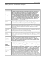
Analysis overview
Construct a network
Rationale: make use of interaction patterns between genes
Identify modules
Rationale: module (pathway) based analysis
Relate modules to external information
Array Information: Clinical data, SNPs, proteomics
Gene Information: gene ontology, EASE, IPA
Rationale: find biologically interesting modules
Find the key drivers in interesting modules
Tools: intramodular connectivity
(highly related to module membership),
gene significance
Rationale: experimental validation, therapeutics, biomarkers
Page 2 of 20
WGCNA User Manual
Short glossary of network concepts
Term
Definition
Coexpression
network
We define coexpression networks as undirected, weighted gene networks. The
nodes of such a network correspond to gene expressions, and edges between
genes are determined by the pairwise Pearson correlations between gene
expressions. By raising the absolute value of the Pearson correlation to a power
β ≥ 1 (soft thresholding), the weighted gene coexpression network construction
emphasizes large correlations at the expense of low correlations. Specifically, a ij
= |cor(xi , xj )|β represents the adjacency of an unsigned network. Optionally, the
user can also specify a signed co-expression network where the adjacency is
defined as follows: a ij = |0.5+0.5*cor(xi , xj )|β
Module
Modules are clusters of highly interconnected genes. In an unsigned coexpression
network, modules correspond to clusters of genes with high absolute correlations.
In a signed network, modules correspond to positively correlated genes.
Connectivity
For each gene, the connectivity (also known as degree) is defined as the sum of
connection strengths with the other network genes: k i = ∑ u≠i a iu . In coexpression
networks, the connectivity measures how correlated a gene is with all other
network genes.
Intramodular
connectivity
(kIN)
Intramodular connectivity measures how connected, or coexpressed, a given gene
is with respect to the genes of a particular module. The intramodular connectivity
may be interpreted as a measure of module membership.
Module
eigengene
The module eigengene corresponds to the first principal component of a given
module. It can be considered the most representative gene expression in a module.
Example: MEblue (also denoted as PCblue) denotes the module eigengene of the
blue module.
Eigengene
significance
When a microarray sample trait y is available (e.g. case control status or body
weight), one can correlate the module eigengenes with this outcome. The
correlation coefficient is referrred to as eigengene significance. The WGCNA
software outputs the eigengene significance of each module (eigengene) and the
corresponding correlation test p-value.
For each gene, we defined a “fuzzy” measure of module membership by
correlating its gene expression profile with the module eigengene of a given
module. For example MMblue(i)= cor(xi ,MEblue) measures how correlated gene
Module
i is to the blue module eigengene. MMBlue(i) measures the membership of the ith
Membership
gene with respect to the Blue module. If MMBlue(i) is close to 0, then the ith gene
is not part of the Blue module. But if MMBlue(i) is close to 1 or -1, it is highly
also known as
connected to the Blue module genes. The sign of module membership encodes
whether the gene has a positive or a negative relationship with the Blue module
eigengene-based
eigengene. WGCNA also outputs the corresponding correlation test p-value for
connectivity
module membership (denoted by PvalueMMblue). The module membership
(kME)
measure can be defined for all input genes (irrespective of their original module
membership. It turns out that the module membership measure is highly related to
the intramodular connectivity kIN. Highly connected intramodular hub genes tend
Page 3 of 20
WGCNA User Manual
Term
Definition
to have high module membership values to the respective module.
Hub gene
This loosely defined term is used as an abbreviation of “highly connected gene.”
By definition, genes inside coexpression modules tend to have high connectivity.
Gene
significance
To incorporate external information into the co-expression network, we make use
of gene significance measures. Abstractly speaking, the higher the absolute value
of GS(i), the more biologically significant is the i-th gene. Examples: GS(i) could
encode pathway membership (e.g. 1 if the gene is a known apoptosis gene and 0
otherwise), knockout essentiality, or the correlation with an external microarray
sample trait. A gene significance measure could also be defined by minus log of a
p-value. The only requirement is that gene significance of 0 indicates that the gene
is not significant with regard to the biological question of interest. The GS can
take on either positive or negative. When the user specifies a microarray sample
trait y (e.g. case control status or a quantitative outcome), WGCNA defines the
gene significance measure as follows GeneSignificance(i)=cor(xi ,y).
Module
significance
Module significance is determined as the average absolute gene significance
measure for all genes in a given module. This measure is highly related to the
correlation between module eigengene and the outcome y.
Construction of weighted gene co-expression networks and
modules
Genes with expression levels that are highly correlated are biologically interesting, since they imply
common regulatory mechanisms or participation in similar biological processes. To construct a
network from microarray gene-expression data, we begin by calculating the Pearson correlations for
all pairs of genes in the network. Because microarray data can be noisy and the number of samples
is often small, we weight the Pearson correlations by taking their absolute value and raising them to
the power ß. This step effectively serves to emphasize strong correlations and punish weak
correlations on an exponential scale. These weighted correlations, in turn, represent the connection
strengths between genes in the network. By adding up these connection strengths for each gene, we
produce a single number (called connectivity, or k) that describes how strongly that gene is
connected to all other genes in the network. We use the general framework of weighted gene coexpression network analysis presented in (Zhang and Horvath 2005, Horvath et al 2006). Briefly, the
absolute value of the Pearson correlation coefficient is calculated for all pairwise comparisons of
gene-expression values across all microarray samples. The Pearson correlation matrix is then
transformed into an adjacency matrix A, i.e., a matrix of connection strengths by using a power
function. Thus, the connection strength (adjacency) a(i,j) between gene expressions x(i) and x(j) is
defined as a(i,j)=|cor(x(i),x(j))|^β.
Optionally, WGCNA can also be used to construct a signed network, which keeps track of the sign
of the correlation coefficient: a(i,j)=|0.5+0.5*cor(x(i),x(j))|^β.
Page 4 of 20
WGCNA User Manual
Because microarray data can be noisy and the number of samples is often small, we weight the
Pearson correlations by taking their absolute value and raising them to the power β.
The resulting weighted network represents an improvement over unweighted networks based on
dichotomizing the correlation matrix, because (i) the continuous nature of the gene coexpression
information is preserved and (ii) the results of weighted network analyses are highly robust with
respect to the choice of the parameter β, whereas unweighted networks display sensitivity to the
choice of the cutoff. The network connectivity k(i) of the ith gene expression profile x(i) is the sum
of the connection strengths with all other genes in the network, i.e. it represents a measure of how
correlated the i-th gene is with all the other genes in the network.
To determine the power β used in the definition of the network adjacency matrix, we make use of the
fact that gene expression networks, like virtually all types of biological networks, have been found to
exhibit an approximate scale free topology (Albert et al 2000).
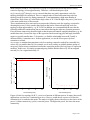
To choose a particular power β, we used the scale-free topology criterion described in (Zhang and
Horvath 2005).
-1.5
-2.0
log10(p(k))
-1.0
-0.5
beta= 6 , scale free R^2= 0.88 , slope= -1.61 , trunc.R^2= 0.98
0.8
1.0
1.2
1.4
1.6
1.8
log10(k)
Figure: Assessing the scale free topology of a weighted gene co-expression network (constructed
using β=6). If the dots form an approximate straight line relationship then the network forms a scale
free network. The black curve corresponds to the regression line with model fitting index R^2. The
red curve describes a truncated exponential fit (see Zhang and Horvath 05) for more details.
Scale free topology criterion (this technical section may be skipped at first reading).
The network exhibits a scale free topology if the frequency distribution p(k) of the connectivity
follows a power law: p(k)~k-γ. (Incidentally, the power gamma has nothing to do with the soft
threshold beta that is used to define the co-expression network). To visually inspect whether
approximate scale-free topology is satisfied, one plots log(p(k)) versus log(k). A straight line is
indicative of scale-free topology. To measure how well a network satisfies a scale-free topology, we
use the square of the correlation between log(p(k)) and log(k), i.e. the model fitting index R^2 of the
linear model that regresses log(p(k)) on log(k). If R^2 of the model approaches 1, then there is a
straight line relationship between log(p(k)) and log(k). Many co-expression networks satisfy the
scale-free property only approximately.
Page 5 of 20
WGCNA User Manual
6 7 8 9 10
12
14
16
18
1
20
500
0.4
0.6
Mean Connectivity
3
1000
0.8
4
0.2
2
3
2
4
0
Scale Free Topology Model Fit,signed R^2
5
1500
1.0
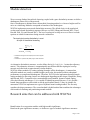
Most biologists would be very suspicious of a gene co-expression network that does not satisfy
scale-free topology at least approximately. Therefore, a soft threshold power β (in
a(i,j)=|cor(x(i),x(j))|β) that give rise to a network that does not satisfy approximate scale-free
topology should not be considered. There is a natural trade-off between maximizing scale-free
topology model fit (scale free fitting parameter R^2) and maintaining a high mean number of
connections. High values of β often lead to high values of R^2. But the higher the power β, the lower
is the mean connectivity of the network.
These considerations have motivated us to propose the following scale-free topology criterion for
choosing the power β: Only consider those powers that lead to a network satisfying scale-free
topology at least approximately, e.g. R^2>0.80. In addition, we recommend that the user take the
following additional considerations into account when choosing the adjacency function parameter.
First, the mean connectivity should be high so that the network contains enough information (e.g. for
module detection). Second, the slope of the regression line between log(p(k)) and log(k) should be
negative (typically smaller than -2). In practice, we find the relationship between R^2 and β is
characterized by a saturation curve. In most applications, we use the lowest power β where
saturation is reached.
As a caveat, we mention that sometimes scale free topology cannot be reached for reasonably low
values of β (say smaller than 20). For example, severe array outliers or globally distinct groups of
arrays may lead to strong correlations between the expression profiles (and very large co-expression
modules). In this case, we simply recommend going with the default choice of β: for an unsigned
network β=6, for a signed network β=12.
1
5
10
15
Soft Threshold (power)
20
5 6
7 8 9 10
5
10
12
14
16
15
18
20
20
Soft Threshold (power)
Figure a) Scale free topology fit (R^2, y-axis) as a function of different powers. In many (but not all)
applications, one observes a saturation type curve. Here we would choose a power of 6 since the
saturation level is reached at this point. The analysis is highly robust with respect to the choice of the
power. b) Mean connectivity (y-axis) versus the power. The higher the power, the lower the mean
connectivity.
Page 6 of 20
WGCNA User Manual
Module detection
We use average linkage hierarchical clustering coupled with a gene dissimilarity measure to define a
dendrogram (cluster tree) of the network.
Once a dendrogram is obtained from a hierarchical clustering method, we choose a height cutoff to
arrive at a clustering. Modules correspond to branches of the dendrogram
WGCNA implements two network dissimilarity measures. The default choice is the topological
overlap matrix based dissimilarity measure (Ravasz et al 2002, Zhang and Horvath 2005, Li and
Horvath 2006, Yip and Horvath 2007). The use of topological overlap serves as a filter to exclude
spurious or isolated connections during network construction.
The topological overlap dissimilarity is used
as input of hierarchical clustering
a
iu auj
TOM ij 
aij
u
min(ki , k j )  1  aij
DistTOM ij  1  TOM ij
•
•
Generalized in Zhang and Horvath (2005) to the case of weighted
networks
Generalized in Yip and Horvath (2006) to higher order interactions
As alternative dissimilarity measure, we also define dissA(i,j)=1-a(i,j) (i.e., 1 minus the adjacency
matrix). This alternative measure is computationally much faster than the topological overlap
measure and often leads to approximately similar modules.
WGCNA defines modules by cutting (pruning) branches off the dendrogram. A common but
inflexible method uses a static (constant) height cutoff value; this method exhibits suboptimal
performance on complicated dendrograms. Therefore, WGCNA also implements dynamic branch
cutting methods for detecting clusters in a dendrogram depending on their shape (Langfelder, Zhang
and Horvath 2007). Compared to the constant height cutoff method, dynamic branch cutting
offers the following advantages: (1) it is capable of identifying nested clusters; (2) it is flexible branch shape parameters can be tuned to suit the application at hand; (3) they are suitable for
automation. WGCNA implements two types of dynamic branch cutting method. The first only
considers the shape parameters. The second method is hybrid method that combines the advantages
of hierarchical clustering and partitioning around medoids.
Research aims that can be addressed with WGCNA
Identification of co-expression modules with high module significance.
Based on the gene significance measure, we define two types of module significance measures.
Page 7 of 20
WGCNA User Manual
The first type is simply the average gene significance of the module genes. The second type of is
referred to as eigengene significance, which is only defined for a microarray sample trait y.
When a microarray sample trait y is available (e.g. case control status or body weight), one can
correlate the module eigengenes with this outcome. The correlation coefficient is referred to as
eigengene significance. WGCNA also outputs the eigengene significance of each module (eigengene)
and the corresponding correlation test p-value.
Identification of intramodular hub genes.
Intramodular connectivity can be interpreted as a fuzzy measure of module membership. Thus, a
systems biologic gene screening method that combines gene significance and connectivity (module
membership) measure amounts to a pathway based gene screening method. Empirical evidence
shows that the resulting systems biologic gene screening methods can lead to important biological
insights (Horvath et al 2006, Carlson et al 2006, Gargalovic et al 2006, Ghazalpour et al 2006).
Fuzzy module annotation of the genes
Apart from detecting co-expression modules, WGCNA also provide a comprehensive annotation of
all genes on the array with regard to module membership. For each gene, the module membership
table reports the module membership with regard to the identified modules. Instead of forcing genes
into distinct modules, the fuzzy module assignment allows the user to identify genes that may be
close to two or more modules. These fuzzy module annotation tables form a resource for biomarker
discovery. The annotation tables can also be used to determine how close a given gene of interest is
to the identified modules. We report both the module membership measure (correlation between the
gene expression profile and the module eigengene) and the corresponding correlation test p-value.
Functional enrichment analysis of module genes
It is natural to use the module membership measure to come up with lists of genes that comprise the
module. For example, one could select blue module genes on the basis of MMBlue>0.6 or
MMBlue< -0.6. Alternatively, one could select the 200 genes with highest absolute module
membership values. The selected genes could be used as input of a functional enrichment analysis
software (EASE, KEGG, Webgestalt, Ingenuity, etc).
For example, we often use the software EASE (David)
http://david.abcc.ncifcrf.gov/summary.jsp
Relating modules to each other and to a microarray sample trait
WGCNA also outputs the module eigengenes in a separate file.
By correlating the module eigengenes one can determine how related (co-expressed) the modules are
to each other. Module eigengenes form the nodes of an eigengene network (Langfelder and Horvath
2007), which may reveal that modules are organized into meta-modules (clusters of co-expressed
modules). The module eigengenes can also be used as covariates of a multivariate regression models
that regresses the microarray sample trait y on the eigengenes.
Installation requirements
1. Windows operating system (Win2000, NT, WinXP or Vista) with .NET Framework installed.
NET Framework could be freely downloaded from Microsoft windows update.
2. All necessary software is listed in the file “WGCNA_Installation_Guide.doc”, which is
included in WGCNA package. Please follow the installation steps.
Page 8 of 20
WGCNA User Manual
3. There’s no hardware requirement for running WGCNA. However, considering the
computation task of network construction, we recommend computers with CPU frequency higher
than 2.0 GHz and memory bigger than 2 GB.
Detailed description of the analysis steps
1. Load data
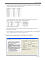
User should specify the “Expression Data” file location first. It’s a comma or tab delimited file
where rows are genes (probe sets) and columns correspond to microarray samples. The first
column should contain gene identifiers.
(Example expression data)
In order to screen for genes or modules that are biologically significant, WGCNA needs to define
a gene significance measure.
Option 1: based on a correlation with a microarray sample trait T that corresponds to a column in
the trait file as “Sample Trait Data” file.
Then GeneSignificance(i)=|cor(Gene i, T)|; the trait could be a binary outcome (case/control
status) or a quantitative outcome (body weight)
Option 2: based on pre-defined gene significance measure that corresponds to a column in the
gene information file. It must contain the same gene sets as in the expression data.
Page 9 of 20
WGCNA User Manual
In order to proceed, the user needs to load a trait file or a gene info file, or both. In the next step,
the user can choose a column of the trait file as sample information trait or a column of the gene
info file as pre-defined gene significance measure.
(Example trait data)
“Gene information Data” file can contain additional gene information like gene names,
chromosome location etc that user wants to keep in the analysis.
(Example gene information data)
Please follow the data format as in sample files. WGCNA can take either comma or tab
delimited text file as input.
After loading the expression data and trait data (or gene information data), user should click the
“Next->” button in order to move to data “Preprocess” step.
2. Data preprocessing and Im Feeling Lazy analysis
First, the user needs to specify how the gene significance measure should be defined.
Page 10 of 20
WGCNA User Manual
For example a microarray sample trait (e.g. a numeric outcome) can be chosen from the sample
trait file. If there is more than one trait in the trait data, user needs to choose a certain trait to be
used for gene significance calculation. As an alternative, user can also specify a pre-defined gene
significance column in gene info data. WGCNA automatically detects whether a column is
numeric (denoted by “N”) or character (denoted by “C”). Please make sure to choose a numeric
column as trait or gene significance values.
Alternatively, the user can choose a pre-specified gene significance measure from the gene
information file. For example, the pre-specified gene significance measure indicates pathway
membership, knock-out essentiality, or the T-test statistic from a prior study.
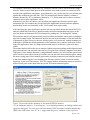
After specifying the gene significance measure, the user can either choose the manual WGCNA
analysis (which allows the user to identify modules and select intramodular hub genes) or the
user can choose and automatic WGCNA analysis by pushing the “I’m feeling lazy” button.
The automatic analysis will automatically choose modules and rank the entire genes according to
network screening results. The automatic analysis has one major advantage: it can deal with tens
of thousands of genes. However, the user does not get to see a cluster tree, module heatmaps etc.
Although we find that the default parameters of the automatic (lazy) analysis work quite well in
many real applications, there is a danger that a module may be an artefact e.g due to an array
outlier.
The manual analysis allows the user to interact with the program regarding module detection and
gene selection but it can only deal with relatively few genes (on our laptop computer fewer than
3600 genes). Since module detection is computationally intensive, the user can filter genes based
on the variance (across the microarrays) and the user can select the most connected genes among
the most varying genes. Since module genes tend to be highly connected, restricting the analysis
to the most connected genes is a reasonable gene filtering criterion (when it comes to module
detection). At the end of the analysis, WGCNA outputs module membership measures which are
defined for all genes in the input data (not just the 3600 most connected genes).
Figure: To proceed with the automatic or the manual WGCNA analysis.
(1). the automatic analysis (“I’m feeling lazy”) uses default parameters for finding modules and
significant hub genes. For each gene and each module, WGCNA outputs a module membership
(MM) value. MM values close to 1 or -1 suggest that the gene is a member in the respective
Page 11 of 20
WGCNA User Manual
module. By using “I’m feeling lazy”, WGCNA will include all the available genes in its analysis,
regardless of their variance or connectivity. Regarding to the output of the automatic analysis,
please refer to the “5. Gene Selection” section for details.
(2). the manual WGCNA analysis allows the user to proceed in a step-wise fashion to define
modules and significant genes. In general, we recommend the manual analysis but it has a
limitation: only 3600 genes can be included for the module definition.
3. Network Construction
First, the user needs to specify whethe a signed or an unsigned gene co-expression network
should be constructed. Asigned network defines modules as clusters of positively correlated
genes. An unsigned network defines modules based on the absolute value of the correlation
coefficient.
To construct a weighted network, a power (soft threshold) larger than or equal to 1 should be
specified. Raising the co-expression similarity to this power would result in a weighted coexpression network. The default power for an unsigned and a signed network is 6 and 12,
respectively. To choose a power, the WGCNA also implements plots for the scale free topology
criterion (Zhang and Horvath 2005). This criterion is described in a separate section.
The “power selection” button results in a graph of scale free topology fit (R^2, y-axis) versus
different power (x-axis). Choose the smallest power for which R^2>0.8 or if a saturation curve
results, choose the power at the kind of the saturation curve.
The button “ClusterSamples” can be used to assess whether arrays are outliers (average linkage
hierarchical cluster tree, Euclidean distance). If the dendrogram has two or more very distinct
branches or outlying arrays, the scale free topology criterion may be meaningless (low R^2
values). In this case, simply choose a power (e.g. 6) or consider removing outlying arrays before
proceeding.
Page 12 of 20
WGCNA User Manual
Once the user have chosen a power, the “next” button will automatically create a weighted coexpression network and a corresponding cluster tree, which will be used for module detection.
The default network dissimilarity measure is based on the topological overlap matrix (TOM). A
less time consuming alternative is to use check box “Use Adjacency instead of TOM”.
Because calculation of TOM or adjacency matrix is very time consuming, WGCNA allows user
to skip this step by un-checking “Re-Calculate Adjacency/TOM”. It’s particularly useful when
user switch back to Step 2 to pick another trait or gene significance column for analysis without
re-calculating the same gene network.
After choosing power, user can click “Next->” button to move to module detection step.
4. Module Detection
WGCNA implements three different approaches for defining modules based on a hierarchical
clustering tree of the genes. All of the three methods required a minimum module size setting.
1) The static branch cutting method simply defines modules as branches that lie below the
height corresponding to the y-axis of the cluster tree.
2) The dynamic height branch cutting method automatically chooses a height cut-off for each
branch based on the shape of each branch (Langfelder et al, Bioinformatics 2007)
3) The dynamic hybrid method is a hybrid between the dynamic method and partitioning around
medoid (PAM) clustering.
The button “Plot Module Significance” plots the average gene significance for each module. The
user can go back to step 2 to specify a different gene significance (GS) measure in the gene info
file or pick a different clinical trait (column) in the sample trait file. In this way, the user can
Page 13 of 20
WGCNA User Manual
study module significance based on different significance measurements without re-calculating
TOM (needs to keep “Re-Calculate Adjacency/TOM box unchecked).
The module merge functions allow the user to manually or automatically merge closely related
modules. User can go ahead to merge close modules using “Merge 2 modules” function. Besides,
“Auto Module Merge” offers an automatic module merging process.
Once modules are defined, user can generate module significance plot by clicking “plot module
significance”. And the “plot cluster tree” button offers an easy way to re-draw hierarchical tree
and module definitions without conducting module detection again.
And the “plot ME Pairs” function plots the relationship between module eigengenes. It’s useful for
studying module similarities, and help merging similar modules. Message: the module eigengenes
(first PC) of different modules may be highly correlated. WGCNA can be interpreted as a
biologically motivated data reduction scheme that allows for dependency between the resulting
components. Compare this to principal component analysis that would impose orthogonality
between the components. Since modules may represent biological pathways there is no biological
reason why modules should be orthogonal to each other.
Page 14 of 20
WGCNA User Manual
With modules detected, user can click “Next->” button to move to gene selection step.
5. Gene Selection
Based on the userr module significance analysis from the previous step, please choose a module
of interest first.
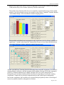
The user can use a heatmap button to plot the standardized expression values of the module
genes (rows) across the arrays (columns). The top row shows the heatmap of the brown module
genes (rows) across the microarrays (columns). The lower row shows the corresponding module
eigengene expression values (y-axis) versus the same microarray samples. Note that the module
eigengene takes on low values in arrays where a lot of module genes are under-expressed (green
Page 15 of 20
WGCNA User Manual
color in the heatmap). The ME takes on high values for arrays where a lot of module genes are
over-expressed (red in the heatmap). ME can be considered the most representative gene
expression profile of the module.
These plots may allow the user to understand the meaning of the module. High values of the
module eigengene suggest that the module is “up” in the corresponding sample. If the correlation
structure of the module is due to a single array, the array may be an outlier.
Gene selection:
It can be useful to study the relationship between gene significance and intramodular
connectivity K using the button “Plot Gene significance versus intramodular connectivity”.
The scaled version of the intramodular connectivity K/max(K) turns out to be highly related to
the corresponding module membership measure. K measures how centrally located the gene is
inside the module.
Page 16 of 20
WGCNA User Manual
To select genes, the user can set the threshold parameters and manually output the genes that
meet the selection criterion. (The user can also save the list to a file). Or the user can choose
automatic gene selection procedure, which selects genes based on their gene significance and
their membership to significant modules.
In gene selection step, user can generate heat map for each specific module. The sample order is
exact the same as in expression data.
“Auto Gene Selection” function allows user to obtain a gene lists with most significant genes
ranked by putting both gene significance and intra-modular connectivity into consideration.
Gene selection output files
Both “I am feeling lazy” and “auto gene selection” functions generate two files as output. They
are of the same format.
(1). Analysis using Trait data
Output contains two different files
1) “LazyGenelist.csv” which contains results for each gene (rows)
2) “MEResults...csv” which contains results for each array sample.
LazyGenelist.csv contains the following columns:
Module membership information, see the columns MM.blue, etc
For each gene and each automatically detected module, WGCNA outputs a module membership
(MM) value. E.g, if a gene has an MMblue value close to 1 or -1, the gene is assigned to blue
module.
Module colors are assigned according to module size: turquoise denotes the largest module, blue
next, then brown, green, yellow, etc. The color grey is reserved for non-module genes.
Cor.Weighted denotes the weighted network estimate of the standard correlation cor(x[i],y)
between the i-th gene and the outcome y. It use of module membership info as well as the
module eigengene significance.
Analogously, p.Weighted is a “weighted” version of a p-value, and q.Weighted is a weighted
version of a q-value (local false discovery rate, see the qvalue library in R). Z.Weighted is a
weighted version of the Fisher Z transform of a correlation coefficient.
In order to learn about which module eigengenes affect the calculation of these measures,
WGCNA also provides the file “MEResults”, which reports the values of the module eigenes
(columns) for different arrays (rows). The top two rows in the file MEResults reports the
eigengene significance of each module.
(2). Analysis using gene significance data
Page 17 of 20
WGCNA User Manual
Output contains two different files
1) “LazyGenelist.csv” which contains results for each gene (rows)
2) “MEResults...csv” which contains results for each array sample.
LazyGenelist.csv contains the following columns:
Module membership information, see the columns MM.blue, etc
For each gene and each automatically detected module, WGCNA outputs a module membership
(MM) value. For example, if a gene has an MMblue value close to 1 or -1, the gene is assigned
to the blue module.
Module colors are assigned according to module size: turquoise denotes the largest module, blue
next, then brown, green, yellow, etc. The color grey is reserved for non-module genes.
GS.Weighted is the weighted network estimate of the corresponding pre-defined GS measure.
GS.Weighted takes account of module membership information and the hub gene significance
measure (HGS) of each module.
The file MEResults reports the module eigengenes (columns) across the arrays (rows).
The top two rows in the file MEResults report the hub gene significance of each module.
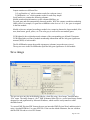
Save image
The user can save any plot in the display panel to a local file using “Save Image” function under
“File” menu. The image format is “emf”. EMF (Enhanced Meta File) is a vector-based image format
designed for and popularized by Microsoft Windows, which could be easily transfer to other
desirable format.
To convert EMF files into PDF format, the user can insert the EMF file into Word, and then print it
using “Acrobat PDFWriter” to crate a PDF file. If the user has Adobe Illustrator, the user can then
edit the PDF file and save it to EPS format.
Page 18 of 20
WGCNA User Manual
How to access help
If needs to read help for current step, the user can display the help by click the “Show Help” menu
under “Help”.
Network function library update
WGCNA utilizes a set of network functions, which is included in the WGCNA package called
“NetworkFunctions-WGCNA.library”. Since we keep updating the library, please download the
latest version from our website. The user can check the versions of both WGCNA program and its
network library using “About WGCNA” menu under “Help”.
In order to update the network library, the user can simple download the latest version and save it to
“C:\WGCNA” folder.
Recovery from unexpected errors
If WGCNA crashes due to any unexpected error, please use “Windows Task Manager” to kill the
R server process, whose name is displayed as “STATCO~1.EXE”. Otherwise, the user may
encounter error like “Unable to create metafile” when the user re-run WGCNA.
Page 19 of 20
WGCNA User Manual
References














Albert R, Jeong H, Barabasi AL (2000) Nature 406:378-382).
Carlson MRJ, Zhang B, Fang Z, Mischel P, Horvath S, Nelson SF (2006) Gene Connectivity,
Function, and Sequence Conservation: Predictions from Modular Yeast Co-Expression
Networks. BMC Genomics 2006, 7:40 (3).
Fuller TF, Ghazalpour A, Aten JE, Drake TA, Lusis AJ, Horvath S (2007) Weighted Gene
Co-expression Network Analysis Strategies Applied to Mouse Weight, Mamm Genome
18(6):463-472.
Dong J, Horvath S (2007) Understanding Network Concepts in Modules. BMC Systems
Biology 2007, June 1:24
Gargalovic PS, Imura M, Zhang B, Gharavi NM, Clark MJ, Pagnon J, Yang W, He A,
Truong A, Patel S, Nelson SF, Horvath S, Berliner J, Kirchgessner T, Lusis AJ (2006)
Identification of Inflammatory Gene Modules based on Variations of Human Endothelial
Cell Responses to Oxidized Lipids. PNAS 22;103(34):12741-6
Ghazalpour A, Doss S, Zhang B, Wang S, Plaisier C, Castellanos R, Brozell A, Schadt EE,
Drake TA, Lusis AJ, Horvath S (2006) Integrating Genetic and Network Analysis to
Characterize Genes Related to Mouse Weight. PloS Genetics. Volume 2 | Issue 8 | August
Horvath S, Zhang B, Carlson M, Lu KV, Zhu S, Felciano RM, Laurance MF, Zhao W, Shu,
Q, Lee Y, Scheck AC, Liau LM, Wu H, Geschwind DH, Febbo PG, Kornblum HI,
Cloughesy TF, Nelson SF, Mischel PS (2006) "Analysis of Oncogenic Signaling Networks in
Glioblastoma Identifies ASPM as a Novel Molecular Target", PNAS | November 14, 2006 |
vol. 103 | no. 46 | 17402-17407
Langfelder P, Zhang B, Horvath S (2007) Defining clusters from a hierarchical cluster tree:
the Dynamic Tree Cut library for R. Bioinformatics. November/btm563
Langfelder P, Horvath S (2007) Eigengene networks for studying the relationships between
co-expression modules. BMC Systems Biology. BMC Syst Biol. 2007 Nov 21;1(1):54
Li A, Horvath S (2006) Network Neighborhood Analysis with the multi-node topological
overlap measure. Bioinformatics. doi:10.1093/bioinformatics/btl581
Miller JA, Oldham MC, and Geschwind DH (2008) A Systems Level Analysis of
Transcriptional Changes in Alzheimer's Disease and Normal Aging. J. Neurosci. 28: 14101420
Oldham M, Horvath S, Geschwind D (2006) Conservation and Evolution of Gene Coexpression Networks in Human and Chimpanzee Brains. PNAS. 2006 Nov
21;103(47):17973-8
Yip A, Horvath S (2007) Gene network interconnectedness and the generalized topological
overlap measure. BMC Bioinformatics 8:22
Zhang B, Horvath S (2005) "A General Framework for Weighted Gene Co-Expression
Network Analysis", Statistical Applications in Genetics and Molecular Biology: Vol. 4: No.
1, Article 17
Page 20 of 20