1
A Flexible Electronic Graph Paper
Version 4.01
User’s Guide
James Tappin
[email protected]
February 2012
Contents
1
3
Introduction
3
1.1
What is it? . . . . . . . . . . . . .
3
1.2
Why is it? . . . . . . . . . . . . .
3
1.3
Requirements . . . . . . . . . . .
4
1.4
Copyright etc. . . . . . . . . . . .
4 4
Getting Started
8
3.1
Making sure it’s there . . . . . . .
8
3.2
Invoking it . . . . . . . . . . . . .
9
3.2.1
Keywords . . . . . . . . .
9
A quick tour of the main window .
9
3.3
Datasets
4.1
2
Main features
5
2.1
Version 2.1 . . . . . . . . . . . .
6
2.2
Version 3.0 . . . . . . . . . . . .
6
2.3
Version 3.04 . . . . . . . . . . . .
6
2.4
Version 3.08 . . . . . . . . . . . .
6
2.5
Version 3.09 . . . . . . . . . . . .
7
2.6
Version 4.00 . . . . . . . . . . . .
2.7
Version 4.01 . . . . . . . . . . . .
4.2
11
General comments . . . . . . . . 11
4.1.1
Observational data . . . . 11
4.1.2
Functions . . . . . . . . . 11
Entering 1-D observational data . 12
4.2.1
From a File . . . . . . . . 12
4.2.2
From IDL top-level variables . . . . . . . . . . . 12
7
4.2.3
Via the data editor . . . . 14
7
4.2.4
With the mouse . . . . . . 14
1
2
GRAFFER
4.3
4.4
4.5
4.6
4.2.5
A note on limits . . . . . . 15 7
Control
4.2.6
Copying another dataset . 15
7.1
Hard Copy . . . . . . . . . . . . . 35
Entering 2-D observational data . 15
7.2
Saving and dumping . . . . . . . 38
4.3.1
From top-level variables . 16
7.3
Opening a new file . . . . . . . . 39
4.3.2
From a file . . . . . . . . 16
7.4
Options... . . . . . . . . . . . . . 39
4.3.3
Copying another dataset. . 17
7.5
Exit and Help . . . . . . . . . . . 40
Entering functions . . . . . . . . . 17
4.4.1
The Editors . . . . . . . . 17 8
4.4.2
Copying another function
4.4.3
Fit dataset
4.4.4
Read function from file . . 20
9.1
Interface . . . . . . . . . . . . . . 41
Dataset selection and manipulation 20
9.2
Arguments . . . . . . . . . . . . . 42
4.5.1
Selection . . . . . . . . . 20
9.3
Keywords . . . . . . . . . . . . . 42
4.5.2
Manipulation . . . . . . . 21
9.4
Restrictions . . . . . . . . . . . . 44
4.6.2
. . . . . . . . 19
9
40
GRAFF_ADD (interface user programs to GRAFFER)
41
1-Dimensional data . . . . 23 10 GRAFF_PROPS (set GRAFFER file
properties programmatically)
44
2-Dimensional data . . . . 24
10.1 Interface . . . . . . . . . . . . . . 44
File-wide settings
5.1
18
Accelerator Keys
Display style . . . . . . . . . . . 23
4.6.1
5
35
27
10.2 Arguments . . . . . . . . . . . . . 45
General settings . . . . . . . . . . 27
10.3 Keywords . . . . . . . . . . . . . 45
5.1.1
Plot annotation . . . . . . 27
10.4 Restrictions . . . . . . . . . . . . 47
5.1.2
General style . . . . . . . 28
Geometry . . . . . . . . . 28 11 GRAFF_PRINT (Make a hard copy of
a GRAFFER file)
47
5.1.4 Key or legend . . . . . . . 29
11.1 Interface . . . . . . . . . . . . . . 47
Axis settings . . . . . . . . . . . . 31
11.2 Argument . . . . . . . . . . . . . 47
5.1.3
5.2
6
Text
33
11.3 Keywords . . . . . . . . . . . . . 48
Version 4.01
12 GRAFF_UPDATE
3
48
13.2 Keywords . . . . . . . . . . . . . 51
12.1 Interface . . . . . . . . . . . . . . 48
13.3 Notes . . . . . . . . . . . . . . . 51
12.2 Arguments: . . . . . . . . . . . . 48
12.3 Keywords: . . . . . . . . . . . . . 48 A Useful procedures
51
12.4 Restrictions: . . . . . . . . . . . . 50
B .grafferrc
13 GRAFF_EXPORT
52
50
13.1 Arguments . . . . . . . . . . . . . 51 C X Resources (X windows systems only) 52
1
Introduction
1.1
What is it?
The first question to be addressed is “What is GRAFFER?”.
GRAFFER is a package of IDL routines for generating and editing plots of data and/or functions.
The primary purpose is the generation of X-Y plots, but as of version 2 there is limited support for
displaying 2-D datasets as contours or in an “image” format, this support is much improved in 3.x
versions.
The plot editing is controlled via a Graphical User Interface (GUI) which allows you to change scalings, annotations etc. and to add & delete traces and even to edit the actual data. Hard copies can be
generated and spooled. The whole plot can then be saved in a GRAFFER file for future editing.
GRAFFER is not and does not pretend to be a fully-fledged drawing tool (there are plenty of those
around e.g. xfig or commercial products) but rather tries to do the things that they (well xfig at
any rate) don’t do well i.e. plotting data.
1.2
Why is it?
The earliest versions of GRAFFER were developed for my own use as a consequence of the amount
of time I was wasting adjusting the format of plots to go into papers (e.g. redoing plots with log axes
or with different ranges). Naturally being of a tinkering turn of mind I gradually added features until
GRAFFER became a reasonably general data-plotting tool.
At about that time a user posted an enquiry to the UseNet group comp.lang.idl-pvwave as to
whether there was a widget-based graph plotting tool in IDL12 . As a result of this GRAFFER version
1
2
This was well before iTools, or even Live_Tools existed.
Unfortunately I don’t have a record of who it was.
4
GRAFFER
1.03 was released to the world.
1.3
Requirements
GRAFFER is written in IDL and needs at least version 5.x to work as it uses pointers and possibly some relatively recent routines. You will need a workstation or terminal which supports one of
the IDL widget devices3 with the X-windows Motif widgets, the graffer main window needs about
900x700 pixels on the screen.
For full functionality you will need a 3-button mouse or something that looks like one to IDL.
In principle GRAFFER ought to run on any system with a reasonably recent version of IDL and
widgets, the current version is tested on IDL 6.4 on Solaris and Linux.
1.4
Copyright etc.
Usage: GRAFFER and its component routines may be freely used, copied & distributed but please:
• Don’t claim you wrote it.
• If you do modify it, make it clear which bits you’ve changed and don’t say I made the
changes.
• Let me know of any improvements you make, and I’ll consider including them in future
releases (credited of course).
Warranty: NONE—You didn’t pay any money for it, I don’t get paid for working on GRAFFER so
you take your chance:
• If it’s useful: GOOD
• If it isn’t: you got what you paid for.
Updates & Maintenance: I’ll try to fix any bugs; but I can’t undertake to add new features unless I
can easily see a way of doing them without a major reconstruction of the internal workings of
GRAFFER (or they seem such good ideas that it’s worth making the effort).
3
N.B. I’ve not tested it on Windows or MacOs as I don’t have access to IDL on these systems.
Version 4.01
2
5
Main features
In this section some of the principal features of GRAFFER are listed.
• Plot a arbitrary number of X-Y plots on a single set of axes (there may be two alternate Y
scales).
• Data for each plot can be:
– Read from a file
– Taken from IDL variables (normally at the $MAIN$ program level only)
– Entered with a data editor
– Entered with the mouse
• Functions can be plotted, including doing basic fits to existing data plots.
• Contour or “image” display of Z vs. X & Y (data or function).
• Easy to change plot limits, log/linear scaling and other axis options.
• Time labelling of axes.
• A secondary Y-axis may be used to allow the overlay of plots with substantially different scales
but the same independent variable.
• Wide range of display styles for individual traces.
• Generate Postscript or EPS version of plot.
• Combining or re-ordering of traces within GRAFFER.
• All possible combinations of error bars and limits are available.
• Save plot to a file for future additions or modification.
• Add a key or legend.
• For X-windows use the IDL RESOURCE="Graffer" key to allow user-customisation of
colours.
6
2.1
GRAFFER
Version 2.1
The main purpose of Release 2.1 was to fix an incompatibility problem which prevented the file
selector compiling under IDL version 5. (Essentially IDL has changed the name of the call to the
system file dialogues under Windows & MacOS and since even code which is never accessed has to
have resolvable names, the Unix version fails to compile with a syntax error).
In addition to this fix, there are a few new options:
• Automatic update can be disabled, this is a convenience if you ware working over a dial-up line
or other slow link.
• A general comment can be added to the whole file.
• A few settings are stored in a .grafferrc file in your home directory. This is at present a
very limited facility.
2.2
Version 3.0
Version 3.0 replaces the obsolete HANDLE constructs with POINTER constructs. In addition may of
the home-made dialogue boxes have been replaced with the system dialogues. The user interface has
been generally tidied up.
2-D datasets can now have 2-D x and/or y values (i.e. non-uniform grids).
2.3
Version 3.04
Version 3.04 adds support for isotropic axes, inverted colour tables for 2-D greyscale and colour plots,
and for setting the display options for 2-D datasets in graff_add. Some crash bugs are also fixed.
Accelerator keys are added to major actions in the main menu.
2.4
Version 3.08
Version 3.08 adds (inter alia): local colour tables for 2-D datasets (will only work properly on displays with more than 8-bits;, significant improvements to the graff_add script (notably support
for getting datasets from files) and a new graff_update script; the settings for 2-D datasets are
displayed in the main window instead of being pop up windows; for colour PostScript output, CMYK
colour decomposition is supported. There are also some internal streamlining changes and several
crash bugs are fixed.
Version 4.01
2.5
7
Version 3.09
Version 3.09 adds support for a secondary Y-axis.
2.6
Version 4.00
• Improved file format. See the Format manual for details. The new format is much more robust,
and it will be possible to read files from any 4.x (or above if that ever happens) with any 4.x
version of the code. Old files can still be read, even version 1.x
• Internal changes especially for contours (to remove artificial limits no longer present in IDL).
• Actually implement colour menu choice.
• Improved font handling for annotations (Can select any hardware (PS) font or TrueType font
known to IDL).
• Allow plot to be displayed in the aspect ratio of the hard copy.
• Rationalize coordinate transform management.
• GRAFF_UPDATE can change data.
• Add GRAFF_EXPORT
• New lines now shown when adding/moving points by mouse.
• Option to only display the current dataset.
• Options to hide individual 2-D datasets (i.e. like colour=omit for ordinatary datasets).
2.7
Version 4.01
• Rename FUNC[XYZ] keys as [XYZ]_FUNC in GRAFF_ADD and GRAFF_UPDATE. (The old
names are accepted with a warning).
• Remove calls to ROUTINE_NAMES and replace with SCOPE_* calls.
• Allow export of data values to IDL top-level variables.
• Add a chooser for import of top-level variables, and in appropriate cases allow import from
other levels.
• Add options to copy another dataset to the current.
8
GRAFFER
• Add method to insert points or prepend them using the mouse.
• Add extra discrete colours.
3
Getting Started
3.1
Making sure it’s there
In order to be able to run GRAFFER, the directory containing the GRAFFER routines must be in
your IDL search path4 . For the purposes of this section I will assume that the GRAFFER directory
is /contrib/idl/graffer but you should substitute the real path name. Note also that the
examples given here are for Unix systems and other systems will be somewhat different but as I don’t
have any other systems I’m not going to do any guessing.
The extension can be done in one of two ways:
Modifying !PATH explicitly: This is probably the safer method, but has to be redone each time you
invoke IDL.
IDL> !PATH = ’/contrib/idl/graffer:’ + !PATH
IDL> graffer
Via the IDL_PATH environment variable: If you know what you are doing this is probably better
but you need to be aware that IDL_PATH must include the default IDL libraries as well as the
GRAFFER libraries.
These examples are in C-shell or TC-shell code:
• When you already have IDL_PATH defined:
$ setenv IDL_PATH /contrib/idl/graffer/:${IDL_PATH}
• When IDL_PATH is undefined:
$ setenv IDL_PATH /contrib/idl/graffer/:+/usr/local/lib/idl
This has the advantage that you only need to run the command once.
4
I suppose you could write a batch file to compile them all by explicit path, but I don’t recommend such things.
Version 4.01
3.2
9
Invoking it
Once you are in IDL with the GRAFFER routines available it is very simple to start GRAFFER, just
type graffer at the IDL> prompt. This will produce a chooser widget which will allow you to
select an existing GRAFFER file, or type in the name of a new file. When you have the file you want
click on the OK button.
If you wish to skip this step, then give the name of the GRAFFER file as an argument, e.g.
graffer, ’test.grf’ this will load the file test.grf if it already exists, or create it if it
doesn’t5 .
3.2.1
Keywords
GRAFFER can accept a number of keywords to control its operation:
XSIZE & YSIZE: These specify the dimensions of the drawing window. By default it is 600 pixels
square. If you specify a larger size then a scrolled draw widget will be used.
GROUP: This is only really useful if you are writing an application which calls GRAFFER. If a
widget ID is specified as the value of the GROUP key, then when that widget is destroyed, so is
the GRAFFER widget.
DEBUG: If this is set, then information-level messages are enabled (if they were disabled—normally
GRAFFER retains the state of the information-level messages) and if it crashes it does not
return to the caller so you can check out the values of the offending variables.
BLOCK: Start the xmanager in blocking mode (so there is no IDL> prompt while GRAFFER is
running). On possible use for this is if GRAFFER is called from another procedure and you
want to be able to get variables from that procedure (although GRAFF_ADD is usually preferred
in such cases).
RECOVER: Recover an autosave file.
COLOUR_MENU: Make the colour selector menus use colour pixmaps to show the colours rather than
text descriptions.
3.3
A quick tour of the main window
Now that you’ve got GRAFFER running and a file selected, you should see the main GRAFFER
window. Depending on which mode you are operating in, it should look like F IGURE 1. The main
areas of the window are:
5
Actually the file won’t be created until you do a save.
10
GRAFFER
Figure 1: The layout of the main GRAFFER window. (With the dataset tab shown to the right).
Main plotting window: This is where the plot is drawn. For suitable datasets you can operate on the
data using the mouse in the plotting window.
Utility control menu: This is at the top of the control panel and contains the buttons for exiting
GRAFFER, saving the file, printing it, opening new files etc. Immediately below it is a box that
displays the current file and directory, this cannot be changed by the user.
General settings: The settings which apply to the whole plot (title, positioning etc) are set from the
“General settings” box, which is just below the utility controls.
Axis settings: The two axis settings boxes allow you to set the properties of the individual axes.
There is one for the X and one for the Y axis. The secondary Y-axis is enabled by the checkbox
button, and the settings for it are in the secondary tab.
Dataset control: In the alternate tab (shown separately to the right of F IGURE 1) are most of the
items which are concerned with selecting datasets, loading data and setting the format of the
trace.
Information boxes Below the main plot window are two small boxes showing the current cursor
Version 4.01
11
location when it is inside the plot window and a larger box that contains a description of the
function of the widget currently under the cursor.
Save In the lower-right corner is a save button with a “floppy disk” icon that only appears when the
file has been changed.
4
Datasets
4.1
General comments
The basic element of a GRAFFER plot is the DATASET. A dataset corresponds to a trace on the
resulting plot. In the resulting plot all the datasets are plotted on a single set of axes, using a single
scaling. All data-input and “line format” operations operate on the current dataset.
There are four classes of dataset in GRAFFER, divided into two broad types each with two subclasses.
4.1.1
Observational data
An observational dataset consists of tabulated numbers which are entered by the user in one of a
number of ways (see below). The subclasses are:
X-Y data: Also referred to as 1-D data. This is the basic GRAFFER dataset and consists of a set of
tabulated X & Y values with optional error limits.
Z data: Also referred to as 2-D data. This is a rectangular array of Z values and the X & Y values at
which they are measured. Note that the grid must be rectangular but it need not be regular.
4.1.2
Functions
A function dataset is an IDL expression which can be evaluated by GRAFFER. As with observational
data, they are divided by dimensionality.
1-D functions: A 1-D function dataset is an IDL expression which when fed an array returns another
of the same length. [There is also a special case of parametric function datasets where two
expressions are needed.]
2-D functions: A 2-D function, takes 2 1-D arrays as its input and returns a 2-D array.
Note that for any dataset other than the first, the dataset must first be created see below (p. 20).
12
GRAFFER
4.2
Entering 1-D observational data
The usual methods of entering observational data are accessed via the X-Y DATA pulldown menu.
Table 1: The error-bar codes in dataset files.
Code
none
#Y
#X
#YY
#XX
#XY
#XYY
#XXY
#XXYY
4.2.1
Col 3
±Y
±X
−Y
−X
±X
±X
−X
−X
Col 4
+Y
+X
±Y
−Y
+X
+X
Col 5
+Y
±Y
−Y
Col 6
+Y
Default?
2
3
4
5
6
From a File
First create an ASCII file with one line for each datum with value in the order:
X Y "lower X err" "upper X err" "lower Y err" "upper Y err"
Any or all of the error limits may be omitted. The interpretation of the error columns is determined by
an error-bars code which is a line starting with a hash (#) sign and then the appropriate combination
of X’s and Y’s. The possible values are described in TABLE 1. The preferred extension of the file
name is .dat.
To read the file, select the “From file...” option of the “XY data” pulldown. This will generate a file-selector widget which you can use to select the file. When you have the file you want, click
on the “OK” button.
N.B. If the dataset already contains values these will be replaced; if the dataset is a function then a
warning is given.
4.2.2
From IDL top-level variables
Rather than writing the values from a program out to a file and then reading the file back into GRAFFER it is easier simply to transfer the variables straight from IDL’s $MAIN$ program level into
Version 4.01
13
GRAFFER. If you need to get variables from some other level into a GRAFFER plot, you should use
GRAFF_ADD (SECTION 9).
This is done via the “top level variables” option of the “XY data” pulldown. This will
produce a pop-up in which you can enter the names of the variables (or slices) for X, Y and such error
bars as are appropriate. Each entry box also has a Pick... button that allows you to pick from the
available variables.
The error-bar option is selected via a pull-down menu at the bottom of the panel, this selection should
be made before you have entered the names as this controls which entry boxes are enabled. You
should enter a name or slice in each enabled box (the X box may be left empty in which case the
index is used).
When you have set all the fields that you want, click on the Do it button. If you have specified
variables or slices with incompatible lengths, then an error message will be generated and you will be
asked to try again.
N.B. If the dataset already contains values these will be replaced; if the dataset is a function then a
warning is given.
A slice is an array subscript or structure tag. Array subscripts must be constants (i.e. they may not
contain references to other variables). They may however reference system variables and intrinsic
functions. Examples:
[0:8] : Legal
[1,*,4] : Legal
[5:*] : Legal
(*,0) : Legal, but deprecated—obsolete subscript delimiters.
[0:n_elements(x)-1] : Illegal—contains a reference to a variable.
[locs] : Illegal—contains a reference to a variable.
[0:n_elements(!p.multi)] : Legal—but rather silly.
(0,*] : Illegal—mismatched delimiters.
Only the total number of elements in the variable or slice is significant. If the X variable is a scalar
(or 1-element array) and Y has more elements, then X is treated as a stride length.
If it is appropriate, then variables from other levels may be selected by prefixing the variable name
with the level number followed by a colon (e.g. 2:x, N.B. there must not be a space after the colon).
This is really only useful (and the chooser only accesses it) if GRAFFER is called from another
14
GRAFFER
procedure with the /BLOCK keyword specified—in other cases only internal GRAFFER routines are
in the call stack.
Undefined variables, strings, object references and entire structures cannot be plotted. Pointers are
automatically dereferenced (before and after slice extraction). If a complex variable is specified, only
the real part is used.
4.2.3
Via the data editor
If you have the values on a piece of paper (some of us still occasionally make measurements manually
and write them down in a notebook), or if you want to remove some bad values from a dataset then
you can use the dataset editor.
The “Edit values” option of the “XY data” pulldown invokes the data editor. This is just an
IDL text widget in which the values in the current dataset are displayed. The normal selection, cutting
etc. apply.
Below the editor window is a pulldown to select the error limit interpretation. Only those options
appropriate to what GRAFFER thinks is the number of columns are actually selectable. This may not
correspond with the actual number of columns—if this happens either enter a carriage return after the
last line or press the do it button (in the latter case a warning message will replace the displayed
dataset for 5 seconds) and the available error options will be updated, the current value will be set to
the default for the number of columns.
4.2.4
With the mouse
This method useful for removing bad data or for indicating features displayed in a 2-D dataset. This
method of editing a dataset is potentially dangerous, and is disabled by default (you can change
the default via the Options... menu option) and can be enabled for individual datasets via the
Extras menu in the dataset tab.
The three mouse buttons each have a function (this is where the assumption that you have a 3-button
mouse comes in):
Left: Enter a point: for a dataset without errors a point is entered at the position of the cursor; for a
dataset with errors the dataset editor (above) is invoked with the selection point at the end of
the dataset. The position is set at the release of the button. When the button is pressed, if there
is already at least one point in the dataset then the cross-hairs are replaced by a line showing
the new segment.
If the ctrl key is down when the mouse button is pressed and the cursor position is within 5
pixels of a line segment, then the point is inserted between the endpoints of that segment (in
Version 4.01
15
the unlikely event of the point being within 5 pixels of more than one segment, then the closest
is chosen).
If the shift key is down when the mouse button is pressed then the point will be added at the
end of the dataset nearer to the cursor location (this allows you to prepend points).
Centre: Edit a point: for a dataset without errors the point nearest to the cursor when the button is
pressed is moved to the location of the cursor when the button is released; for a dataset with
errors the dataset editor is invoked with the pointer at the point nearest to the cursor. N.B. As a
safety precaution, the cursor must be within 5 pixels of the point. When the button is pressed
then the cross-hairs are replaced by a line showing the updated segment(s).
Right: Delete a point: the point nearest the cursor when the button is released is deleted. N.B. As a
safety precaution, the cursor must be within 5 pixels of the point. A circle is drawn around the
point to be deleted if one is in range.
If ctrl or shift is held down when the button is released, then the action will be cancelled. N.B. this
means that for inserting or prepending points, you must release the modifier key before releasing the
mouse button.
4.2.5
A note on limits
In many situations in the real world, some of the values in a dataset are upper or lower limits. To plot
limits requires that the dataset be defined with asymmetrical error bars. If the value is a lower limit,
then set the upper error to Inf (The IEEE ∞ value), for an upper limit, set the lower error to Inf.
4.2.6
Copying another dataset
If the Copy ... option is selected, then a menu will give you a choice of existing XY datasets to
copy to the current dataset. By default if the current dataset contains data, then only those of the same
type are offered, but this can be overridden by selecting the “Show all” button. A warning will be
given before attempting to overwrite functions or 2-D data.
This is useful (for example) if you have a dataset that you want to plot over an image display, and
you need black and white dashes to make it show up; in that case you could set the original to black
continuous and then make a copy and display that with white dashes.
4.3
Entering 2-D observational data
The entry of 2-D data is somewhat more restricted that 1-D because:
16
GRAFFER
1. A dataset editor for 2-D data would be too unwieldy
2. Mouse editing of 2-D data is clearly not feasible.
Therefore there are only three ways to enter 2-D data, all of which are reached via the 2-d datasets
sub-pulldown of the XY data pulldown.
4.3.1
From top-level variables
This is very like the 1-D case and is reached via the Top level variables option of the 2-D
datasets pulldown. The resulting pop-up menu has three slots for the Z, X & Y variables (and
selector buttons. Z must be an (n × m) array and the X & Y must (if given) be respectively an n or
(n × m)-element and an m or (n × m)-element array; if either or both is not given then the index
number is used. Any degenerate dimensions are ignored, so a (n × 1 × m) array will work (e.g. if
you selected slice [*,5,*] from a 3-D array).
If the X or Y variable is a scalar (or 1-element array) and Z has more elements in that dimension, then
that variable is treated as a stride length.
4.3.2
From a file
Again very similar to the 1-D case but the rules for laying out the file are different in that some
“header” information is needed. The format of the file:
• Line1: 2 numbers giving the number of X and Y values (nx , ny ). If nx is negative, this means
the X array is 2-dimensional, and if ny is negative then the Y array is 2-dimensional.
• The nx or nx × ny X values. These may be spread over any number of lines, but there must be
the correct number and a new-line at the end.
• The ny or nx × ny Y values. These may be spread over any number of lines, but there must be
the correct number and a new-line at the end.
• The nx × ny Z values. Again they may be spread over any number of lines, but there must be
the correct number of values.
Note that there are no error bars on 2-D datasets.
Version 4.01
4.3.3
17
Copying another dataset.
Again very similar to the 1-D case. There is however no “Show all” button as there is only one type
of 2-D dataset.
4.4
Entering functions
Although there are several varieties of function in GRAFFER, the format for expressing them and the
editor used to enter them are very similar for all types. The various function editors are reached via
the Function pulldown which is found adjacent to the XY data pulldown.
4.4.1
The Editors
The four types of function can all be entered via one of the function editors. These all share the
following fields:
Function: A box or boxes in which to enter the function. This must be a valid IDL expression which
returns an array of the same size as its input argument.
Axis Range: two or four boxes to enter the limits over which the function is to be evaluated. If no
values are entered, then the range of the axis of the independent variable is used.
Number of evaluations: One or two boxes to the GRAFFER how many time to evaluate the function
over its range (the default for this is 25, but for straight lines you only need 2 while very wiggly
functions may need many more).
Do it and Cancel: Self-explanatory, the Do it button accepts the new function definition and the
Cancel button rejects it.
The precise details vary according to the type of function being specified:
y = f(x): This is the obvious type of 1-D function. The function entered in the function box
should be an IDL expression with x as the independent variable e.g.:
sin(x)
3.2{*}x^2 - x + !pi
replicate(5.1,n_elements(x))
18
GRAFFER
Note that this last case is necessary as the obvious 5.1 does not return an array6 .
x = f(y): Very similar except that now x is expressed as a function of y so the independent variable should now be y e.g. exp(-y^2) - 0.5.
x =f(t) & y = g(t): Also referred to as a parametric function. There are several important
points here:
• There are now two function boxes to be filled, the first gives x as a function of t and the
second gives y as a function of t. For example to draw a unit circle (or part thereof; see
below) you would need to set the functions as: sin(t) & cos(t).
• The range of evaluation must be given as the parameter is not linked to an axis and so
there is no natural boundary. The default is to go from 0 to 1.
z = f(x,y): The 2-D function entry. This requires a function of both X and Y to be given.
Examples would be:
x * sin(y)
-1./sqrt(((x+.5)^2+y^2)>1e-6) - .5/sqrt(((x-1)^2+y^2)>1e-6) - (x^2 + y^2)
In this latter case, note the use of the limiting operators to flatten out the singularities which will, if
they lie at an evaluation point, cause GRAFFER to crash. Internally, the x and y arrays are converted
into 2-D arrays so that the examples above do return the proper 2-D array of z-values.
As there are two independent variables, there are two sets of limits and two evaluation counts. If
you are on a system with limited memory, remember that the function evaluation requires (at least) 3
arrays of double precision numbers with Nx × Ny points.
4.4.2
Copying another function
The Copy ... option allows you to copy an existing function dataset to the current. As is generally
the case a warning is given before overwriting incompatible datasets. If the current dataset is a
function then by default only functions of the same kind are offered as candidates, but the “Show all”
button allows all functions to be offered.
6
I suppose you could use [5.1, 5.1] but then if you reset the number of evaluations you’d be up a gum tree (at least
temporarily).
Version 4.01
4.4.3
19
Fit dataset
Often, when you have observational or experimental data, you want to fit a function to that data. While
GRAFFER cannot provide a fully general function fitting suite, there are facilities to fit polynomials
and other common variations:
Polynomial: y =
P
ai xi
P
Exponential: y = exp(
Logarithmic: y =
ai xi )
ai ln(x)i
P
P
Power law: y = exp(
ai ln(x)i )
Piecewise linear: This is easier to explain than to write down mathematically. Essentially the data
are fit by a series of straight lines (you say how many and GRAFFER determines the slopes
and the locations of the breaks).
Note that the functional forms do in the case of a first-order fit reduce to the more usual forms it’s just
easier to implement them the way they are given here.
To invoke fitting firstly create a new dataset. Do not under any circumstances attempt to invoke
fitting with the data that you wish to fit as the current dataset, if you do then the original data will be
destroyed!
When you select the fitting option on the function pulldown, a pop-up control panel will appear which
allows you to select which dataset to fit and what kind of fit to do.
The default fitting style is a first-order fit which will appears as a straight line with the current selection
of logarithmic and/or linear axes (e.g. for a log-log plot the default will be a power-law). The order
of the fit for the “conventional” forms is just the maximum value of i, for the “piecewise linear” fit
the order is the number of breaks (i.e. one less than the number of segments).
If you have some known bad points in the dataset, then they can be excluded from the fit by selecting
a slice using the standard IDL syntax for slices (e.g. (4:23)).
The update button allows you to try a fit without destroying the pop-up. By using this you can try
various types of fit and select the best. Note that the χ2 values quoted are meaningful in an absolute
sense only if the dataset being fitted has error bars, however even for datasets without errors they do
provide a relative measure of the quality of the fit.
20
4.4.4
GRAFFER
Read function from file
There is also an option to read a function from a file. This is most likely to be used in conjunction
with the option to save a dataset to a file as a means of transferring complicated functions from one
GRAFFER file to another. Lest you should wish to write a function definition with an editor and then
read it into GRAFFER the format is:
Line 1 A function type code, which gives the Dependent variable, i.e. Y≡ y = f (x), X≡ x = f (y),
XY≡ x = f (t), y = g(t) and Z≡ z = f (x, y).
Line 2 The range over which the function is to be evaluated: 2 numbers except for type Z where 4
are needed.
Line 3 The number of function evaluations: 1 number except for type Z where 2 are needed.
Line 4 The function itself, type XY needs a fifth line with the second function.
4.5
Dataset selection and manipulation
In addition to entering datasets, there are several other operations that need to be performed on them.
These “selection and manipulation” operations are described in the following paragraphs. The controls for the operations are found at the top of the dataset tab on the main window.
4.5.1
Selection
Create new dataset: The New button on the dataset operations menu creates a new empty dataset at
the end of the dataset list into which data or a function can be inserted. The same operation can
be effected via the select option of the Other pulldown and selecting the item <new> in
the pop-up menu.
Select dataset: All operations such as reading data or changing linestyles are applied to the CUR RENT dataset. Therefore you need a mechanism whereby you can make a given dataset current.
The simplest mechanism is via the next and previous buttons which allow you cycle
through the currently defined datasets. This is all very well for GRAFFER files with a handful
of datasets, but for a file with many datasets (the most you are allowed to have is 215 − 1 but
I doubt if you will be seriously inconvenienced by this limit!) this could be rather time consuming, so there is an alternative method: the Other pulldown has an option Select which
generates a pop-up menu with all the datasets listed with their sizes, types and names. To select the required dataset, just scroll the list widget (if necessary) and click on the line for the
Version 4.01
21
dataset you want. The <new> item at the end of the list has the same effect as the New button.
The current selection is marked with an asterisk. The Cancel button destroys the pop-up and
leaves the selection unchanged.
Name: Technically this probably belongs under the heading of “Dataset properties” but conceptually
it is better considered here, both because if its use and the location of its entry point.
A dataset can have a name associated with it. This is an arbitrary string which is used for two
purposes, firstly to identify the current dataset and secondly as a label on any legend or key on
the plot. The entry box below the dataset operations menu displays and also allows you to edit
the name of the current dataset. (The serial number in the adjacent box is not editable.)
The only constraint on the string used for the name is that if you intend to add a key to the plot
then you need to remember that both for the hershey fonts (used on-screen) and for PostScript
fonts (used in hard copy) the exclamation mark is an escape character; see the IDL User’s Guide
for more details.
Only show current DS: This toggle allows you to display only the current dataset (useful in complex
plots). Text strings and the key (if one is present) are also suppressed when this is selected. If
text mode (SECTION 6) is also selected, then only the text strings are displayed. If you try to
print while this option is enabled, then you will be asked whether to print all the datasets or just
the current.
4.5.2
Manipulation
In addition to the basic input and editor operations described in SUBSECTION 4.2- SUBSECTION 4.4,
there are a number of operations which work on whole datasets. These operations are all options of
the Other button in the dataset operations menu.
Delete: Delete the current dataset. There is a confirm pop-up before the dataset is actually destroyed.
The next dataset becomes current, unless the dataset deleted was the last in which case the
previous dataset becomes current.
You cannot delete the only dataset in a file.
Erase: Delete the contents of the current dataset but do not remove its slot in the GRAFFER file.
This can be done to the only dataset in a file.
Sort: Reorder the datasets. This generates a pop-up that allows you to select datasets and move them
to a different location in the list. This can be useful if you want to make sure that one dataset
is drawn before another as datasets are guaranteed to be plotted in sequence. It would also be
useful if you wanted to make the items in the key appear in a more logical order.
22
GRAFFER
To use the pop-up just click on the dataset you want to move; the list will then be updated to
remove the selected dataset and add a “start” placeholder. Then click on the dataset immediately
BEFORE the new location of the dataset. This is likely to be the most convenient way of doing
things until RSI implements “drag-and-drop” in list widgets.
Multiple datasets may be moved in one invocation, but the “Do it” button is disabled when
there is an incomplete move (i.e. after a dataset has been selected but not relocated).
Merge: Join two datasets together. The merge option generates a pop-up menu with two selector
menus each with a list of all the observational datasets in the file.
To use it, first select the dataset to be extended from the left hand panel. This will enable all
the compatible datasets in the right-hand panel, select the one you want to add. There are two
additional options:
1. Sort resultant: If this option is selected, then the X-axis of the resulting dataset will be
sorted.
2. Delete appended: If this is selected, then the second dataset is deleted from the file.
The Cancel and Do it buttons have the expected meaning.
HINT: To make a dataset consisting of two existing datasets, while retaining both the originals: create a “New” dataset and then merge each of the
existing datasets into that dataset.
Write to file: Write the current dataset to an ASCII file in a format that can be read by the Read
from file options of the data and function entry menus. A pop-up will appear to allow you
to specify the filename and directory. If you attempt to overwrite an existing file a confirm
menu will appear to allow you to “back out”.
Copy: Make a new dataset which is a copy of the current dataset. The data values and type are
copied. For functions the functions and evaluation range are copied. Display properties will be
the defaults. The new dataset becomes current.
Export: Export the current dataset to top-level IDL variables. This is only available for data datasets,
not for functions. The variable names are fixed, and are listed in TABLE 2.
To select which Y-axis to use (when a secondary Y-axis is enabled), there is a pulldown menu adjacent
to the input options.
Version 4.01
23
Table 2: Variable names for Exports
Quantity
Name
Types
X variable
GR_X
All
Y variable
GR_Y
All
Z variable
GR_Z
9
Y errors
GR_Y_ERR
1,5,7
Y upper error GR_Y_ERR_U 2,6,8
Y lower error GR_Y_ERR_L 2,6,8
X errors
GR_X_ERR
3,5,6
X upper error GR_X_ERR_U 4,7,8
X lower error GR_X_ERR_L 4,7,8
4.6
4.6.1
Display style
1-Dimensional data
Most of the IDL style options for plot traces are available. These are set with the various entry
windows and pull down menus below the plot window. Note that these options are identical for
functions and for observational data.
Symbol: The symbol to use for plotting the points. The pull down menu has images of the symbols,
and displays the current one on the undisturbed button. The default is a continuous plot. There
are now several extra symbols beyond the default IDL symbol set.
Join: Set the type of line to join the points. This can be straight lines joining the points, a histogram
type line or no line at all. Note that no symbol and no line is allowed and will result in the trace
becoming invisible.
Size: The size to use for the plotting symbols as a multiple of the default size. This is ignored for
continuous or histogram plots. Any floating point value is accepted. The symbol size also
determines the length of the caps on error bars.
Line style: Line style to use for continuous plots, ignored for discrete symbols. The pull down menu
shows the available styles. Error bars are always drawn with solid lines.
Line thickness: The width of the line in terms of the basic line width. Enter any integer (≤ 100) to
set the width. This is used both for continuous plots and for discrete symbols. Note that at least
on the printers I use, there is very little visible difference between a thickness of 1 and of 2.
Colour: The colour is set via a pulldown. Most colours have names, but some for which I couldn’t
think of a description are given as an RGB triple. There is a difference between omit and
24
GRAFFER
white: in the first case, the trace is simple not drawn at all; in the second, it is drawn in the
background colour which will overwrite earlier traces and also take time.
Coordinates: The pull down allows you to select one of three coordinate systems:
Rectangular: The usual X-Y plots.
Polar (rad): Data are r and θ values with the angles being given in radians.
Polar (◦ ): As above but the angles are given in degrees.
When the system is changed, the interpretation of the values changes, the values themselves
are unaltered.
Extra options: The Extra button generates a pulldown that allows the toggling of some special
options:
X-axis sorting: For continuous plots, it is possible to request that GRAFFER sort the x-axis
points into ascending order before plotting them. This is controlled by a 2-valued pull
down menu. Obviously it has no visible effect if discrete symbols are in use.
Clipping: Normally IDL clips plots at the axis box, however there are times when it is desirable to let a plot go over the box. To do this switch the Clip to box option to
Off.
Mouse editing: For observational data it is usually possible to enter, modify and delete points
using the mouse, however this may not be desirable so is disabled by default; you can use
the Mouse editing option to allow the current dataset to be changed with the mouse.
4.6.2
2-Dimensional data
For 2-D data there are far fewer options as to how to plot the data than there are for line plots. The
display options are now collapsed to a single button which allows you to toggle between contours and
an “image” format. In each case, the menu below the choice allows you to set the detailed options.
Contoured display: The contouring menu (F IGURE 2) allows you to specify all the options that can
be used in a contour plot.
Levels: The levels can be either explicit, in which case the levels entry box is enabled as
in (F IGURE 2) and levels can be entered one per line. The sorting of the levels into
increasing order as required by the CONTOUR procedure is handled by GRAFFER.
To use a given number of equi-spaced levels, use the pulldown in the top left to select
Implicit levels, this will disable the levels box and enable the # Levels box in
Version 4.01
25
Figure 2: The datasets panel with (left) contouring options and (right) colour/greyscale options shown.
which you can enter how many contour levels you want. This doesn’t use IDL’s internal level setting routines as they do not allow all of the other options, so it is done by
GRAFFER7 .
Colours: Specify the colours of the colour lines (or fill if requested). Unlike the colour settings for line plots, these are given by index, the interpretation of the indices is given in
TABLE 3. If the number of colour indices given is less than the number of levels plotted,
then the indices are recycled.
Thickness: Specify line thicknesses for the contours.
Styles: Specify the linestyles for the contour lines. These are the standard IDL linestyles,
described in the PLOT keywords documentation.
Filled/Outline: This pulldown allows you to specify filled contours. With a suitable selection
of colours this can be a very effective way of displaying data but for large datasets it is
slow.
HINT: There is a dirty way to get a “Stepped greyscale” effect. Firstly ensure you have the greyscale colour table loaded by GRAFFER (this is not
the same thing as using LOADCT, 0; display the data in “Image” format
and select the grey table there) and then use colour indices selected in
the range 16-143.
7
For real enthusiasts, the levels are determined as levels = rg * (findgen(nl)+.5)/nl + mn where rg is
the range of the data (ignoring infinities & NaNs), mn is the smallest value in the data and nl is the number of levels.
26
GRAFFER
Table 3: The GRAFFER colour indices.
Index
0
1
2
3
4
5
6
7
8
9
10
11
12
13
14
15
16
17
18
19
20
21
22
23
24
25
26
27
Red
255
0
255
0
0
0
255
255
255
127
0
0
127
255
85
170
170
255
0
85
0
85
0
85
170
255
170
255
Green
255
0
0
255
0
255
0
255
127
255
255
127
0
0
85
170
0
85
170
255
0
85
170
255
0
85
170
255
Blue
255
0
0
0
255
255
255
0
0
0
127
255
255
127
85
170
0
85
0
85
170
255
170
255
170
255
0
85
Name
White (BG)
Black (default)
Red
Green
Blue
Cyan
Magenta
Yellow
Orange
#7f ff 00
#00 ff 7f
#00 7f ff
#7f 00 ff
Mauve
Dark Grey
Light Grey
Dark Red
Light Red
Dark Green
Light Green
Dark Blue
Light Blue
Dark Cyan
Light Cyan
Dark Magenta
Light Magenta
Dark Yellow (brown)
Light Yellow
Labelling: IDL allows the labelling of selected contours. GRAFFER doesn’t allow the full
functionality but allows you to label every nth contour. Specifying 0 means don’t label
any contours.
Colour/Greyscale display: Also referred to as “Image” display. To do this, the dataset is warped to
fit the data coordinate system and the resulting image is displayed. While this can make a nice
display it has two serious drawbacks:
Version 4.01
27
1. It is slow, seriously slow on a small machine.
2. It completely obscures all earlier datasets.
When this option is selected, then the “image” options menu (F IGURE 2) is displayed. The
options are rather simpler than those for a contour plot:
Range: The range of values to map from “black” to “white”. If these are both zero, then the
minimum and maximum of the data are used.
Colour table: Select any of the available colour tables; when the menu appears, the current
table will be shown highlighted.
Gamma: The power-law to use in mapping colour indices to the data values (see the LOADCT
& XLOADCT documentation). In essence a value of Γ less than 1 puts most of the colours
at the lower end of the data range.
Pixel size: Because GRAFFER has to warp the dataset to fit the data coordinate system, it has
to create an image array with a colour index for each pixel covered by the “image”; this is
all very well on a screen with typically 0.28 mm pixels but for PostScript with its flexible
pixel size the notional pixel size is very small and hence the resulting image would be
huge. To avoid this problem, you can specify a notional pixel size to be used in making
hard copy. The size is given in mm and the default of 0.5 mm is usually adequate.
Log mapping? Select whether to map the colours logarithmically. Note that this will only
work with a positive-definite dataset or explicit range with both limits positive.
Invert colours? Select whether to map the colours with the high values at the dark end of the
table.
Hidden: If this is selected, then the dataset is not displayed. There are no options.
5
File-wide settings
While the options discussed in the preceding pages have applied only to specific datasets, others apply
to the whole file. These options are set from the general tab to the left of the main plotting window.
5.1
5.1.1
General settings
Plot annotation
The plot titles and subtitles can be entered in the appropriate boxes at the top of the general settings
menus. The only subtlety to be aware of is the IDL plotting string escape sequences (see the IDL
User’s Guide) for specific details. To prevent excessive error messages, the plot is not updated if any
annotation string ends with a single exclamation mark.
28
GRAFFER
5.1.2
General style
The character size and line width settings allow you to specify:
1. The character size for all annotations (the relation between the sizes of the title, subtitle and
axis labels is defined by IDL and GRAFFER does not try to change these (it can be done but
the defaults are pretty good and it would be a horrible job to fit in all the extra setting boxes).
2. The line thickness used for the axes (again in principle you could set the axis line widths
separately but it would usually be ugly and there isn’t room for the controls).
5.1.3
Geometry
For most purposes IDL’s default plotting region is perfectly adequate, and that is what GRAFFER
uses by default. However there are occasions when you need more precise control of the shape of the
plot and the size of its margins. If and when you do need this capability, the Corners... button
generates a pop-up menu to set these options.
There are two ways of specifying the plot geometry:
By region: This sets the corners of the axis box in normalized coordinates. To use this select the
Corners option on the pulldown at the top of the menu and enter the x & y coordinates of the
lower left and upper right corners in the boxes. The Do it button will not be enabled until the
values are legal, so you can’t crash it!
By aspect ratio: This uses David Fanning’s ASPECT routine to define the corners such that the
aspect ratio of the plot is preserved even if it is sent to different shaped pages. To use this
select the Aspect ratio option of the top pulldown and enter the aspect ratio (defined as
the length of the Y axis divided by the length of the X axis) and a margin size. The margin size
is expressed as a fraction of the page size, and this is interpreted such that the smaller margin
will be that large and the other will be as large as needed to achieve the required aspect ratio.
Isotropic: Enabling this check box, forces the scales on both axes to be identical. The actual sizing
of the plot then uses IDL’s defaults. This option is not available when a secondary Y-axis is
enabled.
HC Aspect Ratio: Enabling this check box tells GRAFFER to display the plot on the screen with
the same aspect ratio as it will have in the final hard copy. (This is independent of the other
settings).
To restore the default margin settings, invoke the pop-up and click on the Defaults button
Version 4.01
5.1.4
29
Key or legend
Plots with several traces on them are often useful, but without some explanation no-one other than
the person who drew the plot will know what the traces are. For this reason GRAFFER provides a
mechanism for adding a key to the plot.
Figure 3: The key (or legend) definition menu of GRAFFER.
Pressing the Add key button creates the key definition pop-up (F IGURE 3). The first time you
invoke this (for any given GRAFFER file), the menu will be disabled apart from the Draw a key
on the plot? pulldown at the top; only when that pulldown is set to Yes does the rest of the
menu become accessible. The menu can conceptually be split into two halves. The left-hand side
specifies the properties of the key while the right specifies which datasets are to be included.
The location of the menu is specified by giving the coordinates of the lower left and upper right
corners in one of three coordinate systems:
Data: The coordinates are given in the same coordinate system as the data being plotted. This system
has the property that if you change the axis limits, the key will remain fixed relative to the traces.
If you change the plot geometry (see above), the whole plot will change in a self-similar way.
It is often difficult to figure out just what the box will look like especially in logarithmic plots.
Data coordinates always use the primary Y-axis.
30
GRAFFER
Normalized: The coordinates are given in coordinates which run from (0, 0) in the lower left corner
of the page to (1, 1) in the upper right corner of the page. This means that the key box is
fixed relative to the page and will move relative to the axes if the plot boundaries are moved
and relative to the traces if the plot limits are changed. Strictly these GRAFFER uses “region”
coordinates so that the location is correct when hard-copy aspect ratio is selected.
Frame: This system (which is implemented by GRAFFER not by IDL) is similar to the Normalized
system, but measured relative to the corners of the axis box. This means that the plot behaves
in a self-similar way when you change the boundaries, and the key remains fixed relative to the
axes when you change the limits. With a suitable boundary setting you can put the key outside
the axis box by using coordinates outside the range 0 to 1. This is the default system.
If the default character size is not suitable, then it can be adjusted by entering a scale factor in the
“Character size” box, this is a factor relative to the default (which depends on the size of the axes and
also the global charater size setting).
If you have a secondary Y-axis, then checking the “Show Y side” box adds (l) or (r) after the
description to indicate which axis is applicable to that dataset.
You can arrange the items in the key in any number of columns (although in practice more than 2
tends not to work very well), just enter the number of columns you want in the box.
There are two possible formats for the line sample each of which has advantages and disadvantages:
1 point: Plot a short horizontal line segment (if there are lines) with a single symbol (if any) in the
centre. This is the more compact layout and usually looks better, but it cannot distinguish
normal lines from histogram formats.
2 point: Plot a sloping line segment with a symbol at each end. This needs a little more room and
can look untidy but does distinguish sloping-line traces from histograms. For historical reasons
this is the default.
The format is determined by the 1 or 2 points pulldown. Another pulldown determines if a box
is to be drawn round the key.
If a title is entered in the title box, then this is written above the key, spanning all columns for a
multi-column key.
The right-hand side of the menu is a selector menu to determine which datasets will be listed in the
key, only the 1-D datasets (observations and functions) are listed. In addition to the buttons for the
individual datasets, there is an All button which selects all the datasets (you can then deselect the
ones you don’t want).
Version 4.01
31
Unfortunately it is not possible to provide a dynamic update to the key on the plot, so to see what it
looks like you need to click on Do it and then try again if it doesn’t work. Note that datasets with a
colour of Omit are not included even if they are selected (but they will appear as soon as the colour
is changed).
5.2
Axis settings
The settings for the two axes are identical and so I will only describe a generic axis setting. Almost
all of the standard IDL axis styles are available along with a number of extensions.
Enable secondary Y-axis? (Y-only) This check box is used to enable/disable the secondary Y-axis.
When it is disabled, then the contents of the “secondary” tab are desensitised, as is the Y-axis
selector on the dataset menu.
Main/Secondary (Y-only) Tabs to select whether to adjust the primary or secondary axis.
Label: The axis label can be entered via the label box. Remember that the exclamation mark is an
escape character (see IDL User’s Guide); to reduce the number of error messages, the label is
not updated if the string ends in a single exclamation mark.
Logarithmic/Linear: This is set by a toggle pulldown.When logarithmic is chosen, if one of the
limits (see below) is zero or negative, the plot will not be updated until the limit is changed.
Style: This pulldown covers a multitude of sins, including but not limited to the IDL [XY]STYLE
key settings. Each option generates a further pulldown of sub-options. Where appropriate, the
selected sub-option is indicated by an asterisk.
Exact range: By default IDL (and hence GRAFFER) rounds the axis limits to some “nice”
range which covers the requested axis range. If however you really want an exact range,
this can be forced by setting the exact range option to On.
Extended range: If this is switched on the the axis is extended by a small amount (5%) from
the requested limits. This operates after the any rounding.
Draw axes: Normally IDL draws an axis on each side of the plot (thus producing a full box).
Both axes can be turned off by setting this option to Off.
Draw box axis: Turning this option to Off just suppresses the axis to the right or above the
plot. If the draw axes option is turned off then it has no effect. This option is disabled for
the Y-axes when a secondary Y-axis is enabled.
Minor ticks: GRAFFER does not have room to provide full support for arbitrary control of
the number of minor tick marks. If this option is set to On (the default) IDL determines
the number of minor ticks to add, when it is Off then minor ticks are suppressed.
32
GRAFFER
Annotations: This option allows the suppression of the normal labelling of the axis.
Time labelling: Normally only used on the X-axis, but you might want it on Y and it’s easier
to provide the option than to omit it8 . This option provides some support for labelling an
axis with times. When it is switched On then a pop-up appears to ask you the units in
which the time is given, what is the largest unit you wish to put on the plot (e.g. if the
values are in hours, you might want to label the axis in days and hours) and the label to
give to the zero point (this is given in the largest unit displayed—the idea behind this is to
allow a date to be added to an axis whose times are in hours of a given day). The largest
supported unit is days.
Example: Suppose you have a time series lasting a couple of days starting on 24 February 1997 and the times are given in hours from 00:00 UT
on 24 Feb. The you should set the time unit to hours, the “display to”
unit to days and the zero value to 24. You should them label the axis
(say) February 1997.
Origin Axis: If this option is turned on, then add an axis going through the origin of the other
axis (if that is on the plot). If the draw axes option is off then the axis will be labelled
with the axis label, normally it will not be labelled. For the X-axis this option is disabled
if a secondary Y-axis is enabled. For the Y-axis, annotations are suppressed if an origin
axis is selected for both Y-axes.
Grid: If this is set to a line style, then extend the major tick marks to form a grid and draw
them with the given style.
Autoscale: This isn’t really a style option as such, but a means of updating the axis limits (see
below) to accommodate the data. There are two possible ways to do this:
Extend: This will increase the upper limit, or decrease the lower limit so as to include
all the datasets within the range.
Extend or shrink: This will also raise the lower limit or lower the upper limit to remove
blank space.
In either case for Y-axes, if a secondary axis is enabled, then only those datasets plotted
against that Y-axis are scanned.
Limits: The Min and Max boxes allow you to set the axis range. If the range requested is invalid,
then the plot will not be updated until a valid range is entered (this prevents GRAFFER crashing
while you are editing the numbers). To scale the axis to the data, use the Autoscale option of
the Style pulldown.
8
Because of limitations in the way IDL uses label formatting functions, time labelling is not supported for the secondary
Y-axis.
Version 4.01
6
33
Text
In addition to the standard plot labels and the key options, GRAFFER also has facilities to add text
at arbitrary locations on the plot. To use this facility, you must switch GRAFFER to text mode
which makes it interpret mouse button clicks in the plot window as text operations instead of dataset
operations. The mode button is a pulldown just below the global and dataset tabs. When you are in
text mode, the cross hairs that follow the cursor change from continuous to dashed and extend over
the whole window rather than just the axis box.
The button assignments are essentially the same as for the mouse dataset editing operations, i.e. the
LEFT button adds a new text item at the location of the pointer, the CENTRE button initiates the text
editor on the existing string whose anchor point is closest to the pointer and the RIGHT button deletes
the string whose anchor is nearest the pointer. Both the edit and delete operations have a maximum
distance of 5 pixels. Insertion of new text and editing of existing text are both accomplished via the
same text input pop-up (F IGURE 4). There are many user-settable fields in the menu:
The text string itself: This is a text entry widget into which you can type the text string to be displayed. Any of the IDL graphics controls ( !<char> commands) may be used as these text
strings are displayed in vector fonts (unless of course you have specifically requested hardware
font). As you type the text into the box, it will be reflected in the graphics window above in the
size, font etc. in which it will appear on the plot. If no text string is given it will be displayed
as <NULL>, this will not be printed on a hard copy, nor is it displayed while editing the text.
Also, text items after the current one may not appear while editing is in progress.
Character Size: Enter a floating-point value to give the character size in terms of the default value.
When hard copies are made, the size is adjusted to give the same number of characters across
the page as were on the screen.
Colour: The colour of the text, the pulldown has the same colours as for plot traces, except that there
is no option to omit the text entirely. In the figure the “alternate” colour pixmap selector is
enabled.
Thickness: Enter an integer value to specify the line thickness to be used for the character drawing.
This should be used with caution, but the results in hard copy are usually better than the Xwindows display suggests.
Justification: A pull down which allows you to set Left, Centre, Right or otherwise-justified text.
For non-standard justifications a pop-up with a slider is used to set the justification in the range
0.0 (Left justified) to 1.0 (Right justified).
Orientation: Set the orientation of the text. This is measured in degrees anti-clockwise from the
normal position of parallel to the X-axis and going left to right.
34
GRAFFER
Figure 4: The text input/editing menu of GRAFFER.
Coordinate system: A pull down to select Data, Normalized or Frame coordinates as the system in
which the text is anchored. The default is data, but if you wish the text to remain in the same
place on the page when you change the axis range, then use normalized, if you want the text
fixed relative to the axes use Frame. For more details of the systems see p 29.
Y-axis: If a secondary Y-axis is available, then this allows you to select which one to use for Data
coordinates. This selector is not created when there is no secondary Y-axis, and is disabled
when the coordinate system is not Data. By default, the coordinate system of the current dataset
is selected.
Version 4.01
35
Position: Set or adjust the position of the anchor point, both X and Y are floating-point numbers and
are given in the currently selected coordinate system.
Font: A pair of pull downs to select the font. The first selects the font group, and the second the
specific font. All the recognized fonts are available—for illustrations of the characters, and
information on the mappings see the “IDL User’s Guide”. For hardware fonts, the rendering in
X will prbably be incorrect and also the orientation will probably not be fully honoured.
In order to reduce the refresh time as you are typing the text string, the plot is not updated after every
character you type, instead the string is displayed in a small window at the top of the text entry menu
(the only characteristic which is ignored is the orientation). To see how it will actually look on the
plot, click on the Update button, this will update the plot without exiting the text menu. The Do it
and Cancel buttons have their usual meanings.
Remember that when you are in text mode you cannot then use the mouse to edit datasets, however
all other dataset operations remain valid.
7
Control
In this section I shall describe the various “control” operations that allow GRAFFER to deal with the
outside world and thus be useful. All of the operations are controlled from the buttons on the top-left
of the GRAFFER control panel.
7.1
Hard Copy
GRAFFER supports the generation of PostScript hard copy files with a wide range of options. When
requesting hard copy you can retain the current options (or the defaults if none have been set) by
selecting the Quick option of the pulldown. If you select the Set up option, then the hard copy
setup menu will be produced (F IGURE 5).
At the top are four pulldown toggle buttons to select:
Monochrome/Colour: Whether to generate colour PostScript or not. The default is monochrome.
In monochrome mode, all line plots appear black, but 2-D data displayed in “image” format
will appear as a greyscale.
Normal/Encapsulated: Normal is just a regular printable PostScript file. Encapsulated is not printable, but can be included into other files e.g. xfig, LATEXetc. The filename ends .ps or .eps
according to the selected option.
36
GRAFFER
Figure 5: The GRAFFER hard copy set up menu. Upper: with regular PS selected; Lower: with
Encapsulated PS selected.
Version 4.01
37
Landscape/Portrait: Describes the orientation of the plot on the page. If encapsulated PostScript is
selected then this is ignored apart from changing the default dimensions.
RGB/CMYK Select which colour representation to use (disabled if monochrome is selected).
The size and placement of the plot can be controlled by the buttons and entry boxes in the next few
lines of the menu:
Paper size: Allows you to toggle between the European A4 (210 × 297mm) (default) and American
Letter (8.5 × 1100 ) paper sizes. As IDL doesn’t put paper size commands into its PostScript
output9 this is just used in GRAFFER’s internal accounting to figure out margins etc.
Centre on page: Adjust the offsets so that the current page size is centred on the paper; note this
is not a retained characteristic so you have to re-apply this any time you change the page
dimensions. (Disabled for EPS).
X & Y sizes: Set the X & Y dimensions of the page. The X & Y directions correspond to the directions of the axes on your plot. Note that there is nothing to stop you making a portrait
orientation file with the X dimension larger than the Y, in fact this is the recommended way of
making landscape encapsulated files.
X & Y offsets: Set the distance between the lower left corner of your plot page and the lower left
corner of the page. Again this refers to the corners as seen when you are looking at the plot
in the usual way people look at plots, GRAFFER handles the axis interchanging needed (but it
will get it wrong if you don’t tell it the right paper size!). (Disabled for EPS).
X & Y remain: These are not user settable, they just tell you how far the top right corner of your
plotting page is from the top right corner of the paper. (Not meaningful for EPS).
The other “formatting” options are:
Plot timestamp: If this is selected, then add a string with the date of generation and the username of
the generator to the plot.
Font: There are two pulldowns that allow you to select any of the PostScript fonts that IDL knows
about (yes even Zapfdingbats!). The first selects the family and the second the weight and
slant. This font is used for titles, axis annotations and labelling, keys and any text strings where
hardware font was selected. Text strings in vector fonts are not affected.
9
This is a good thing as if a file with embedded paper size commands is sent to a printer with different sized paper it
will typically hang the queue until someone intervenes.
38
GRAFFER
The default output file is derived from the GRAFFER file name by replacing the suffix with .ps
or .eps according to the selected output. This can be changed via the output file entry box or the
Pick ... button. The default may be restored with the Default button.
For “normal” PostScript files, GRAFFER will automatically spool the file to the printer. The default
command is lp, this can be changed by entering a new command in the “Spool command” boxes:
the first box is for that part of the command which precedes the filename and the second for anything
that has to come after the filename10 . When encapsulated output is selected, then a PostScript viewer
is selected.
Example: Suppose, you have a printer that needs some special file to be attached to the file to make transparencies so that the command to spool foo.ps
is:
cat upper.ps foo.ps | lp -dEaf-color1
then the two boxes should contain respectively:
cat upper.ps
| lp -dEaf-color1
The Cancel and Do it buttons have their usual meanings.
7.2
Saving and dumping
One of the key features of GRAFFER is that you can save you plot to a file and then come back to it
later. The various saving options are under the File menu, there is also a sub-menu to allow you to
make screen dumps.
There are three save options which allow you to save to the current file in the current format or to
save to a specified file in either binary or ASCII format. Clicking on the “Changed” indicator on the
far right of the control panel does a save to the current file, in the current format.
Normally binary files are preferable as they are smaller and quicker to read and there is no risk of
losing precision in floating point numbers. However if you want to transfer the file to a different
platform then you should use ASCII as the representations of the numbers may differ11 .
10
Originally this was intended for VMS where options such as the print queue name came after the file name.
Unfortunately I was not able to devise an automatic means of distinguishing binary, ASCII and non-GRAFFER files if
I used XDR for the binary form. Abandoning ASCII would have meant that version 1 could not be read into version 2. For
machines with IEEE floating point formats (most machines nowadays) binary files can be read irrespective of endianness
by the simple expedient of checking the version number and swapping bytes if the raw version number is greater then 255.
11
Version 4.01
39
If you request a save to a new name, a pop-up will appear to allow you to edit the new filename. If
you try to save over an existing filename, a warning will be given and you will have the option of
overwriting or trying another name.
The screen dump allows you to dump the GRAFFER plot window to a PNG, TIFF or NRIF file,
the name will be the current filename with an appropriate extension. JPEG is not available as it is a
lossy scheme unsuitable for line plots. There is also an option to start the IDL image save dialogue to
choose any format known to IDL12 .
7.3
Opening a new file
When you start GRAFFER you either give it a file name as an argument, or you use a picker to select
or specify a file name. If you wish to work on another file, you don’t have to leave GRAFFER and
restart as the Open options allow you to change file without exiting.
Open restore: This will start up the same picker that is used when you enter GRAFFER without an
argument. The only difference is that you can’t select a non-existent file.
Open new: This starts a pop-up that allows you to enter the name and directory of a new file. If you
specify a file that already exists, you will be given the opportunity to try something else before
it is overwritten, however the existing file will not be opened.
7.4
Options...
The “Options...” item in the control menu allows you to set a number of options, via a pop-up dialogue
(F IGURE 6).
Show 2-D data Toggles the display of 2-D datasets (allows the display of contour and image data to
be suppressed on slow machines).
Default mouse editing Controls whether mouse editing is allow on new datasets.
Colour selector Whether the colour selector should be text-based or show samples. N.B. This is
only useful with the “Save” option as it cannot be changed once GRAFFER has been started.
Autosave interval Set the number of seconds between automatic saves of the GRAFFER structure.
PDF Viewer Select the program to use to view the PDF help files.
All these values can be saved to the .grafferrc file in your home directory, and also applied to
the current session (except the colour selector type).
12
At least on my installation, although Jpeg2000 is theoretically available it does not actually work.
40
GRAFFER
Figure 6: The options menu dialogue.
7.5
Exit and Help
The Exit item in the File menu exits from GRAFFER to the IDL> prompt, it does not exit from
IDL. If the file is changed, you will be given the opportunity to save it or abort the exit.
The Help button launches a browser to look at a PDF version of this manual. In addition in the main
menu, the text-entry menu, the hard copy menu and the contour menu a brief description of each
operation appears in a message window when the pointer is moved over a user-settable item. (IDL
does not support help balloons13 .)
8
Accelerator Keys
In version 3.04, accelerator keys were added to the main menu.
The following accelerators are defined:
Ctrl-Q Quit.
Ctrl-S Save.
13
No longer true, but they are only available for Draw & Button widgets directly in a base widget
Version 4.01
41
Ctrl-Shift-S Save binary as.
Ctrl-Alt-S Save ascii as.
Ctrl-P Hard copy – quick.
Ctrl-Shift-P Hard Copy – set up.
Ctrl-N Open new file.
Ctrl-O Open existing file.
Ctrl-H Show user manual.
Ctrl-Alt-P Dump draw widget to a PNG file.
Ctrl-Alt-T Dump draw widget to a Tiff file.
Ctrl+Alt+N Dump draw widget to an Nrfi file.
9
GRAFF_ADD (interface user programs to GRAFFER)
This is all very well but suppose you have a procedure that generates radial spokes on a series of
images and you want to use GRAFFER to make up a plot of these radial spokes it’s going to be rather
tedious to specify all the slices to the top-level variable reader, or write them to a series of files and
then load each file. To automate this and indeed to allow the use of variables which are never passed
back to the top-level to be used there is a procedure GRAFF_ADD. GRAFF_ADD adds datasets to
a GRAFFER file, if need be the file is created, it cannot delete datasets or replace existing datasets,
also some of the more complex options cannot be set up by GRAFF_ADD.
9.1
Interface
graff_add, file, [[[z], x,] y, errors=errors, x_func=x_func, $
y_func=y_func, errtype=errtype, z_func=z_func, $
polar=polar, rescale=rescale, /display, join=join, $
style=style, psym=psym, symsize=symsize, colour=colour, $
thick=thick, neval=neval, description=description, $
frange=frange, /graffer, /ascii, /noclip, $
mouse=mouse,z_format=z_format, z_nlevels = z_nlevels, $
z_levels = $
z_levels, z_colours = z_colours, z_style = z_style, $
42
GRAFFER
z_thick = z_thick, z_range = z_range, z_label = $
z_label, z_pxsize = z_pxsize, z_invert = z_invert, $
z_fill = z_fill, z_log=z_log, z_ctable = z_ctable, $
xy_file = xy_file, z_file = $
z_file, func_file = func_file, y_axis=y_axis]
9.2
Arguments
file string The graffer file to modify.
z float The Z values for a 2-D dataset (If only 2 arguments are present, then they are treated as X &
Y)
x float The x values to add.
y float The y values to add.
9.3
Keywords
errors float Array with errors, 1-d or (m,n).
errtype string Specify error types as code see TABLE 1
x_func string Function specification for x = f(y) or x = f(t)
y_func string Function specification for y = f(x) or y = g(t)
z_func string Function specification for z = f(x,y)
frange float The range of x, y or t over which to plot a function
polar int If unset or 0 rectangular, 1 = polar in radians, 2 = polar in degrees.
rescale flag If set, then reset the scaling of the plot with the autoscale routine.
display flag If set, then display the plot on the current device.
style int The standard IDL linestyle codes
psym int The GRAFFER symbol code - extended IDL symbol codes
join int The style of joining: 0 - none, 1 - sloping lines, 2 - histogram
symsize float The size for the symbols (relative to standard)
Version 4.01
colour int Colour number - standard GRAFFER colours
thick int Line thickness.
neval int The number of times to evaluate a function. (2-elements for z_func)
description string A description of the data set.
sort flag Whether to sort the values on the X-axis
graffer flag If set, then invoke GRAFFER after adding the dataset.
ascii flag If set, then save as an ASCII GRAFFER file (default is binary)
noclip flag If set, then disable clipping to the axis box.
mouse int If explicitly set to zero then disable mouse-editing of the dataset.
z_format int 2-D datasets, select displayformat (0=contour, 1=colour image)
z_nlevels int For 2D datasets, select number of automatic contours
z_levels float For 2D datasets, select levels for explicit contours
z_colours int For 2D datasets, select the colours for the contours
z_style int For 2D datasets, select linestyles for contours
z_thick int For 2D datasets, select line thicknesses for contours
z_label int Specify the interval of contours for labelling.
z_fill flag If set, then fill the contours.
z_range int For 2-D datasets, specify the cutoff range for image displays
z_pxsize float For 2D datasets, specify the pixel size to use in images for PS device.
z_invert flag For image display, invert the colour table if set.
z_log flag If set, then map the Z values logarithmically.
z_ctable int Select a colour table for 2-D display of images.
xy_file string A file with a graffer dataset (x-y plot).
z_file string A file with a graffer dataset (2-D data).
43
44
GRAFFER
func_file string A file with a graffer function dataset.
y_axis int Select which Y-axis to scale this data to. (Set but ignored if the file does not have a
secondary Y-axis).
9.4
Restrictions
• The func<xyz> keys and the x,y,z arguments are exclusive.
• The GRAFFER key overrides the DISPLAY key and the ASCII key.
• There is no support for deleting or replacing datasets.
10
GRAFF_PROPS (set GRAFFER file properties programmatically)
This procedure is the global counterpart of GRAFF_ADD, and allows you to set various options from
your program.
10.1
Interface
graff_props, file, title=title, subtitle=subtitle, $
charsize=charsize, thick=thick, corners=corners, $
aspect=aspect, comment=comment, xtitle=xtitle, $
xrange=xrange, xlog=xlog, xexact=xexact, $
xextend=xextend, xaxes=xaxes, xbox=xbox, $
xminor=xminor, xtime=xtime, xorigin=xorigin, $
xgrid=xgrid, xauto=xauto, $
ytitle=ytitle, $
yrange=yrange, ylog=ylog, yexact=yexact, $
yextend=yextend, yaxes=yaxes, ybox=ybox, $
yminor=yminor, ytime=ytime, yorigin=yorigin, $
ygrid=ygrid, yauto=yauto, yr_enable = yr_enable, $
yrtitle=yrtitle, $
yrrange=yrrange, yrlog=yrlog, yrexact=yrexact, $
yrextend=yrextend, yraxes=yraxes, $
yrminor=yrminor, yrtime=yrtime, yrorigin=yrorigin, $
yrgrid=yrgrid, yrauto=yrauto, display=display, $
graffer=graffer, ascii=asciih_orient=h_orient, $
Version 4.01
45
h_colour=h_colour, h_eps=h_eps, h_xsize=h_xsize, $
h_ysize=h_ysize, h_xmargin=h_xmargin, $
h_ymargin=h_ymargin isotropic = isotropic, h_cmyk = $
h_cmyk, ctable = ctable, h_print = h_print, h_viewer $
= h_viewer, h_file = h_file
10.2
Arguments
file string The graffer file to modify.
10.3
Keywords
title string Set the plot title.
subtitle string Set the subtitle for the plot.
charsize float Set the character size to be used for axis labelling and plot annotations.
thick int Set the line thickness to be used for drawing the axes.
corners float Set the location of the plot in normalized coordinates by specifying the locations of
the corners (4-elemant array [x0,y0, x1,y1])
aspect float Set the location of the plot within the normalized coordinate system by aspect ratio
and margin (2-element array [aspect, margin] N.B. Specifying both ASPECT & CORNERS is
an error and the plot location is unchanged.
isotropic flag Set the plot to use isotropic coordinates.
comment string Set a descriptive comment for the whole file. (String array)
[x|y|yr]title string Set the title for the specified axis.
[x|y|yr]range double Set the range of the specified axis (2-element array).
[x|y|yr]log flag Set or unset the use of logarithmic axes.
[x|y|yr]exact flag Set or unset the exact range bit of the IDL axis style setting
[x|y|yr]extend flag Set or unset the extended range bit of the IDL axis style setting
[x|y|yr]axes flag Set or unset the axis plotting bit of the IDL axis style setting.
46
GRAFFER
[x|y]box flag Set or unset the "box-axis" bit in the IDL axis style setting. Note this is not applicable to the secondary Y-axis, and is ignored for the main Y-axis if a secondary axis is specified.
[x|y|yr]minor flag If set, then display minor ticks on the plot; if explicitly zero, then turn off
the minor ticks.
[x|y|yr]time flag/struct If set to zero, then turn off time labelling, otherwise this must be a
structure with the members described in TABLE 4.
unit
max_unit
zero
0 == seconds
1 == minutes
2 == hours
3 == days
Gives the unit in which the
time is expressed in the axis data.
gives the largest unit to
display on the plot (same code as
for unit)
gives the value to be used for
the zero of the axis (expressed in
units of max_unit
Table 4: Time axis structure
[x|y|yr]origin flag If set, then plot an axis at the origin.
[x|y|yr]grid flag Make a grid from the major ticks, using linestyle n-1 (0 == no grid).
[x|y|yr]auto flag If set, then perform an autoscale on the specified axis, the corresponding range
setting takes precedence over this setting.
yr_enable flag Enable/disable the display of a secondary Y-axis.
display flag If set, then display the plot on the current device.
graffer flag If set, then invoke GRAFFER after adding the dataset.
ascii flag If set, then save as an ASCII GRAFFER file (by default a binary graffer file is generated).
h_orient int Set landscape(0) or portrait (1) orientation of the page.
h_colour flag Set or unset the generation of a colour (E)PS file.
Version 4.01
47
h_cmyk flag Set or unset the use of the CMYK model for (E)PS files. Specifying this keyword will
force colour (E)PS.
h_eps flag Set or unset the generation of EPS file rather than PS (N.B. if h_eps is set and h_orient
is not specified, then h_orient=1 is implied).
h_[xy]size float Set the X(Y) dimension of the page in cm
h_[xy]margin float Set the X(Y) offset of the page from the lower-left corner of the page.
ctable int Set the default colour table for image display.
h_print string(s) Specify the command to print PS output files (can be a scalar or 2-element aray).
h_viewer string(s) Specify the command to view EPS output files (can be a scalar or 2-element
aray).
h_file string Specify the output file for hardcopies.
10.4
Restrictions
• The ASPECT and CORNERS keys are exclusive (if both are given, both are ignored).
• [X|Y|YR]RANGE overrides [X|Y|YR]AUTO.
• The GRAFFER key overrides the DISPLAY key and the ASCII key.
• As yet the addition/modification of a key (legend) is not supported.
• Not all hardcopy options can be set.
11
11.1
GRAFF_PRINT (Make a hard copy of a GRAFFER file)
Interface
graff_print, file[, <graff_props keywords>]
11.2
Argument
file string The graffer file to modify.
48
11.3
GRAFFER
Keywords
Any keyword accepted by GRAFF_PROPS (See SUBSECTION 10.3) can be used.
12
GRAFF_UPDATE
User-callable interface to update the properties of a dataset.
12.1
Interface
graff_update, file, idx, name=name, polar = polar, rescale = rescale, $
style = style, psym = psym, join = $
join, symsize = symsize, colour = colour, thick = $
thick, neval = neval, description = description, $
sort = sort, ascii = ascii, noclip = noclip, $
mouse = mouse, z_format = z_format, z_nlevels = $
z_nlevels, z_levels = z_levels, z_colours = z_colours, $
z_style = z_style, z_thick = z_thick, z_range = $
z_range, z_label = z_label, z_pxsize = z_pxsize, $
z_invert = z_invert, z_fill = z_fill, z_log = z_log, $
z_ctable = z_ctable, y_axis=y_axis, $
make_current = make_current x_values = x_values, $
y_values = y_values, z_values = z_values, x_func = $
x_func, y_func = y_func, z_func = z_func, xy_file = $ $
xy_file, z_file = z_file, errors = errors, errtype = $
errtype, neval = neval, frange = frange
12.2
Arguments:
file string The graffer file to modify.
idx int input The dataset index to modify (starting at 1).
12.3
Keywords:
name string Find the dataset to update by searching the descriptor fields to match the name.
frange float The range of x, y or t over which to plot a function
Version 4.01
49
polar int If unset or 0 rectangular, 1 = polar in radians, 2 = polar in degrees.
rescale input set, then reset the scaling of the plot with the autoscale routine.
style int The standard IDL linestyle codes
psym int The GRAFFER symbol code - extended IDL symbol codes.
join int The style of joining: 0 - none 1 - sloping lines 2 - histogram
symsize float The size for the symbols (relative to standard)
colour int Colour number - standard GRAFFER colours (which may well not work on current
device).
thick int Line thickness.
neval int The number of times to evaluate a function. (2-elements for z_func)
description str A description of the data set.
sort input to sort the values on the X axis.
ascii input set, then save as an ASCII GRAFFER file (by default a binary graffer file is generated).
noclip input set, then disable clipping to the axis box.
mouse int If explicitly set to zero then disable mouse-editing of the dataset.
z_format int For 2-D datasets, select display format (0=contour, 1=colour image)
z_nlevels int For 2D datasets, select number of automatic contours
z_levels float For 2D datasets, select levels for explicit contours
z_colours int input For 2D datasets, select the colours for the contours
z_style int For 2D datasets, select linestyles for contours
z_thick int For 2D datasets, select line thicknesses for contours
z_label int Specify the interval of contours for labelling.
/z_fill If set, then fill the contours.
z_range int For 2-D datasets, specify the cutoff range for image displays
z_pxsize float For 2D datasets, specify the pixel size to use in images for PS device.
50
GRAFFER
/z_invert For image display, invert the colour table if set.
/z_log If set, then map the Z values logarithmically.
z_ctable int Select a colour table for 2-D display of images.
y_axis int Select to which Y-axis the dataset will be scaled.
/make_current If set, then make the modified dataset into the current dataset when the file is
next opened.
x_values double New X values.
y_values double New Y values.
z_values double New Z values.
x_func string New x=f(y), or x=f(t)
y_func string New y=f(x), or y=f(t).
z_func string New z=f(x,y).
xy_file string File for new 1-D data.
z_file string File for new 2-D data.
errors double New error values.
errtype string Specify error types as code (e.g. "XXY" for asymmetrical errors in X and symmetric errors in Y)
frange float The range of x, y or t over which to plot a function
12.4
Restrictions:
Does not allow the type of dataset to be changed. If neither the index or the name is given, then
the current dataset is modified. Specifying both is an error. If name is given then (1) If there are 2
datasets of the same name, the first will be modified, (2) if the name is not found, then the program
exits without updating.
13
GRAFF_EXPORT
graff_export, file, index, name = name, outfile = outfile
Version 4.01
13.1
51
Arguments
file string The graffer file.
index int The index of the dataset to write.
13.2
Keywords
name string The descriptor of the dataset to write.
outfile string The file to which to write the dataset
13.3
Notes
If neither the index or the name is given, then the current dataset is written. Specifying both is an
error. If name is given then (1) If there are 2 datasets of the same name, the first will be written, (2) if
the name is not found, then the program exits without writing.
Acknowledgements
Thanks to Norbert Hahn of the University of Darmstadt for suggesting the need for a more compact
format for those using the package on small screens. And to Christian Marquand of the Free University of Berlin for providing a fix to the plot symbol pixmaps for little-endian machines. To Phil
Williams of the Children’s Hospital Medical Center, Cincinnati OH for suggesting the revisions of
the compact format. To Simon Plunkett of USRA for the idea of the alternate key format. To Tim
Howard of SwRI for the idea of adjusting font sizes in the key.
A
Useful procedures
This is a quick list of some of the procedures that are part of GRAFFER which are likely to be of use
in other contexts, they are mostly compound widgets which offer some extensions over the versions
in the IDL User’s library:
cw_bbselector A pulldown menu like CW_BSELECTOR, but able to use bitmap labels (you can’t
mix bitmaps and text though).
cw_btgroup Like CW_BGROUP but with tracking events.
52
GRAFFER
cw_pdtmenu Like CW_PDMENU but with tracking events.
cw_pdtsmenu A pulldown menu with options to put a state flag on the lowest-level options.
graff_enter An entry box with rather more options than CW_FIELD (e.g. format, capture focus on
pointing, tracking events).
fractile Return specified percentiles of an array of values.
For more details, use the DOC_LIBRARY procedure. There may be other useful routines that I’ve
missed.
B .grafferrc
The .grafferrc file provides a very limited range of control over the default settings for GRAFFER. It is a colon-separated text file with just five options.
Autosave: float The time between autosave operations in seconds. (300.)
Supp2D: bool Whether to suppress display of 2-D datasets (for slow machines, really a legacy of
the mid-90’s whne GRAFFER was first developed). (0)
MouseEdit: bool Whether to enable mouse editing of data by default. (0)
PDFView: string The program to use to view the PDF help files. (searches for the first of acroread,
kpdf, xpdf, kghostview, gv, okular and evince to be installed)
ColourMenu: bool Whether to use colour pixmaps or text descriptions in the colour selectors. (0)
The usual way to create and modify it is via the Options menu (SUBSECTION 7.4) by selecting Save
or Save and Do.
C
X Resources (X windows systems only)
All the top-level widget bases in GRAFFER have the key resource=’Graffer’ specified. This
allows the user to specify colours for GRAFFER widgets that are different from this of other IDL
widgets. Putting the following into your .Xdefaults makes “lemon yellow” GRAFFER widgets
and light green widgets for other IDL widgets .
Version 4.01
!
!
!
!
This sets the number of colors IDL reserves.
Leave 5 unallocated color
table entries for other applications and
the windowing system:
Idl.colors:
-5
Idl*background: palegreen
Idl*text*background: lightcyan
Idl*button*background: lightcyan
Idl*slider*background: lightcyan
Idl*list*background: lightcyan
Idl*droplist*background: lightcyan
! These are specific to Graffer
Idl*Graffer*background: \#ffff88
Idl*Graffer*text*background: white
Idl*Graffer*button*background: white
Idl*Graffer*slider*background: white
Idl*Graffer*list*background: white
53
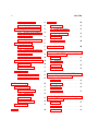


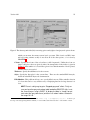
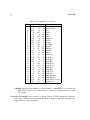

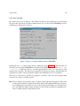
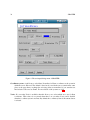
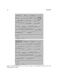
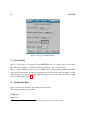


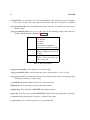



![hank yo_fo buyil_gaSamsung (}a_Te_a ]hs](http://vs1.manualzilla.com/store/data/005691502_1-2e8e29ffb67d0c8f7d0d701e3cb644b7-150x150.png)