Download Dr. Charlie Mayne`s NMR Lab Manual

Fundamentals
of
High Resolution
Pulse and Fourier Transform
NMR Spectroscopy
iii
Table of Contents
Part I
Lecture Notes
1.
2.
3.
4.
5.
6.
7.
8.
9.
10.
11.
12.
The Nuclear Zeeman Effect. .................................................................................
1.1.
A magnetic field breaks the degeneracy of nuclear spin states. ...............
1.2.
The differences in level populations are very small. ................................
Net Magnetization and Nuclear Precession. .........................................................
2.1.
Classical Equation of Motion of a Magnetic Dipole. ...............................
2.2.
Magnetization of an Ensemble of Spins. ..................................................
2.3.
Nuclear Precession....................................................................................
Detection of Precessing Magnetization ................................................................
The Rotating Frame. ...........................................................................................
The Effects of Radio Frequency Fields—Pulses. ...............................................
5.1.
On Resonance Pulses. .............................................................................
5.2.
Off Resonance Pulses. ............................................................................
Relaxation—Bloch's Equation. ...........................................................................
6.1.
Correlation Functions and Spectral Densities.........................................
6.2.
Relaxation Mechanisms. .........................................................................
The CW NMR Experiment. ................................................................................
The FT NMR Experiment. ..................................................................................
The Anatomy of a Free Induction Decay. ...........................................................
9.1.
FID of a Single Resonance. ....................................................................
9.2.
FID of Two or More Lines......................................................................
9.3.
Digitization of Free Induction Decays....................................................
9.4.
Time Averaging. .....................................................................................
Digital Filters and Convolution. .........................................................................
10.1. The Convolution Theorem......................................................................
10.2. Deconvolution.........................................................................................
10.3. Truncation of the FID. ............................................................................
10.4. Apodization.............................................................................................
10.5. Sensitivity Enhancement.........................................................................
10.6. Resolution Enhancement. .......................................................................
10.7. Lorentzian to Gaussian Transformation..................................................
Decoupling and the Nuclear Overhauser Effect. ................................................
11.1. Equation of Motion for a Two Spin System. ..........................................
11.2. Homonuclear Decoupling. ......................................................................
11.3. Broadband Decoupling. ..........................................................................
Multiple Pulse Experiments, Spin Echoes, Measurement of T1 and T2. ............
12.1. Measurement of T1 by Inversion Recovery. ...........................................
12.2. Hahn Spin Echoes. ..................................................................................
1/8/01
3
3
3
5
5
5
6
8
10
12
12
13
15
16
18
21
23
25
25
25
26
29
35
35
37
37
37
37
39
40
41
41
43
44
45
45
46
iv
12.3. Measurement of T2 by the Carr, Purcell, Meiboom, Gill Method. ......... 46
13.
Polarization Transfer, INEPT and DEPT. ........................................................... 48
13.1. INEPT. .................................................................................................... 48
13.2. DEPT....................................................................................................... 48
14.
Fundamental Concepts of Two Dimensional NMR. ........................................... 53
14.1. The Generic 2D Pulse Sequence............................................................. 53
14.2. The Two Dimensional Fourier Transform.............................................. 54
14.3. Phase Sensitive 2D NMR........................................................................ 55
14.4. Phase Cycling.......................................................................................... 57
14.5. Pulsed Field Gradients. ........................................................................... 61
15.
Chemical Shift Correlation Experiments. ........................................................... 62
15.1. Homonuclear Shift Correlation (COSY). ............................................... 62
15.2. Carbon-Carbon Homonuclear Correlation, the 2D INADEQUATE Experiment.
63
15.3. Heteronuclear Chemical Shift Correlation.............................................. 66
16.
Homonuclear and Heteronuclear J-Spectra. ....................................................... 68
16.1. Heteronuclear J-Spectra.......................................................................... 68
16.2. Homonuclear J-Spectra........................................................................... 68
17.
A Basic Pulsed Fourier Transform Spectrometer. .............................................. 71
17.1. Generating B0—The Magnet.................................................................. 72
17.2. Generating B1—the observe transmitter................................................. 72
17.3. Detecting the Nuclear Induction Signals—the Receiver. ....................... 72
17.4. The Data Processing and Spectrometer Control
System—the Computer........................................................................... 72
17.5. Maintaining a Constant Field/Frequency Ratio—the Lock System. ...... 72
17.6. Generating B2—the Decoupler............................................................... 72
17.7. Controlling the Sample Temperature—the Variable
Temperature System. .............................................................................. 72
17.8. Coupling All the Other Subsystems to the Sample—the Probe. ............ 72
17.8. Bibliography ....................................................................................................... 73
Part II
Laboratory Experiments
Part II Introduction. ........................................................................................................
Laboratory 1: Proton Line shape, Proton Resolution. ...................................................
1.1.
Demonstration.........................................................................................
1.2.
Pertinent Parameters and Commands. ....................................................
1.3.
Setting Up, Shimming, the Line Shape Test...........................................
Laboratory 2: Observation of Carbon-13. ......................................................................
2.1.
New Commands and Parameters. ...........................................................
2.2.
Observation of an X Nucleus..................................................................
2.3.
Calibration of Observe Channel Pulse Widths. ......................................
2.4.
Determination of a Carbon T1.................................................................
1/8/01
77
79
79
80
80
85
85
85
86
88
v
Laboratory 3:
3.1.
3.2.
3.3.
3.4.
Laboratory 4:
4.1.
4.2.
4.3.
4.4.
Laboratory 5:
Laboratory 6:
Laboratory 7:
Decoupling and the NOE. ....................................................................... 95
New Commands and Parameters. ........................................................... 95
Homonuclear Single Frequency Decoupling. ......................................... 95
Heteronuclear Single Frequency Decoupling. ........................................ 96
Gated Decoupling and the NOE. ............................................................ 97
Observation of a Less Common X Nucleus .......................................... 101
New Commands and Parameters. ......................................................... 102
Outside preparation............................................................................... 102
General Considerations......................................................................... 104
PROCEDURE:...................................................................................... 104
Distortionless Enhancement by Polarization Transfer (DEPT) ............ 107
Homonuclear Correlation Spectroscopy (COSY). ................................ 111
Double Quantum Filtered Homonuclear Correlation
Spectroscopy (DQCOSY). .................................................................... 115
Laboratory 8: Heteronuclear Chemical Shift Correlation
Spectroscopy (HETCOR). .................................................................... 119
Laboratory 9: Indirect Detection of Heteronuclear Chemical Shift
Correlation (HMQC, HMBC). .............................................................. 123
Laboratory 10:Heteronuclear Two Dimensional J–Spectroscopy. ............................... 127
Laboratory 11:13C Two Dimensional INADEQUATE, Direct Detection of
Carbon-Carbon Bonds. ......................................................................... 129
Laboratory 12:Through Space Correlations (NOESY). ............................................... 131
Part III
Appendices
Appendix 1: Locking and Shimming the Spectrometer. ..............................................
1.1.
Obtaining Lock. ....................................................................................
1.2.
Shimming the Magnet...........................................................................
Appendix 2: Sample Preparation .................................................................................
Appendix 3: Solutions to Problems. .............................................................................
1/8/01
137
137
139
141
143
vi
1/8/01
Part I
Lecture Notes
by
Charles L. Mayne
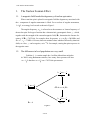
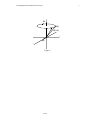
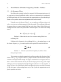
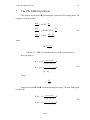
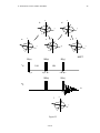
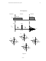
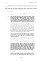
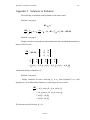
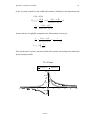
1. The Nuclear Zeeman Effect.
3
1.
The Nuclear Zeeman Effect.
1.1.
A magnetic field breaks the degeneracy of nuclear spin states.
When a nuclear spin is placed in a magnetic field the degeneracy associated with
the z component of angular momentum is lifted. For a nucleus of angular momentum,
I = 1 2 , two energy levels result as shown in Figure 1.
The angular frequency, ω 0 , is referred to as the resonance or Larmor frequency of
the nuclear spin. Each type of nucleus has a characteristic gyromagnetic factor, γ , which,
together with the strength of the external magnetic field, B0 , determines the Larmor frequency. If B0 = 7.05 Tesla , for example, then, for protons, ν 0 = ω 0 2π = 300 MHz , and
for 13 C , ν 0 = 75 MHz . Of course, these are nominal values which are affected by chemical
shifts, etc. Also, γ can be negative, as in 15 N for example, causing the spins to precess in
the opposite sense.
1.2.
The differences in level populations are very small.
Problem 1: A certain sample has 1 million chloroform molecules.
At 300 K using Boltzmann statistics, how many fewer protons will have
m = −1 2 than have m = 1 2 on a 7.05 Tesla spectrometer.
I = 12 , m = − 12
I = 12 , m = ± 12
β
∆ E = hω 0 = hγ B 0
I = 12 , m = + 12
B0 = 0
B0 > 0
Figure 1
2/13/01
α
4
Part I: Lecture Notes
Answer:
kT = 4.14 × 10 −14 erg
∆E = 1.99 × 10 −18 erg
∆E
= 4.8 × 10 −5
kT
 5 × 10 5 − δ 2 
∆E 
exp −
= 0.999952 = 

 kT 
 5 × 10 5 + δ 2 
δ = 24
2/13/01
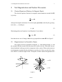
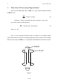
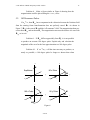
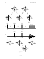
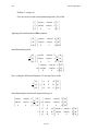
2. Net Magnetization and Nuclear Precession.
5
2.
Net Magnetization and Nuclear Precession.
2.1.
Classical Equation of Motion of a Magnetic Dipole.
The classical equation of motion for a magnetic moment, µ, in an external field, B,
is given by:
dp
= ×B
dt
(1)
where p is the angular momentum. For nuclear spins, p and µ are related by the gyromagnetic ratio, γ , according to:
= γp
(2)
Eliminating p between Equation (1) and Equation (2) one obtains:
d
= γ ( × B)
dt
(3)
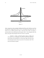
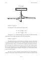
Note that the time rate of change of µ is always perpendicular to µ and B. See Figure 2.
2.2.
Magnetization of an Ensemble of Spins.
Now suppose one has an ensemble of moments, i , each making an angle, θ , with
the external field (the external field direction will be taken to be the z direction), but randomly distributed with respect to their components in the xy plane. When nuclear spins are
treated quantum mechanically they distribute in just this way if they are placed in a magnetic field for a sufficient length of time. The dipoles will have identical magnitudes but a
B0
0
θ
µ
= +1/2
= -1/2
Figure 2
2/13/01
6
Part I: Lecture Notes
few more will have a positive z component rather than a negative one. This corresponds to
the excess of nuclear spins having m = 1 2 over those having m = −1 2 . (See Figure 2.)
Summing over all the i , one has:
∑ i = M0
(4)
i
M0 is usually referred to as the thermal equilibrium magnetization.
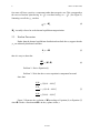
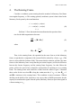
2.3.
Nuclear Precession.
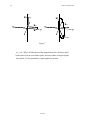
Rather than the thermal equilibrium distribution described above, suppose that the
i are arbitrarily distributed such that
∑i = M
(5)
dM
= γ (M × B)
dt
(6)
i
then it is easy to show that
Problem 2: Derive Equation (6).
Problem 3: Write the above vector equation in component form and
show that
(
)
d Mx
= γ M y Bz − Mz By
dt
d My
= −γ ( M x Bz − Mz Bx )
dt
d Mz
= γ M x By − M y Bx
dt
(
(7)
)
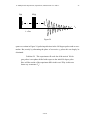
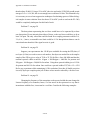
Figure 3 illustrates the evolution of M according to Equation (6) or Equation (7)
when B is in the z direction and M is in the yz plane at time, t.
2/13/01
2. Net Magnetization and Nuclear Precession.
7
z
Bo
M(t)
M(t+dt)
y
dM
x
Figure 3
2/13/01
8
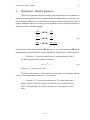
3.
Part I: Lecture Notes
Detection of Precessing Magnetization
In the case where B = B0k = Bzk and M(t = 0) = M0i = M xi the equation of motion
for M reduces to
(
)
dM
= γ M y Bzi − M x Bz j
dt
(8)
Problem 4: Satisfy yourself that the above equation is correct and
prove that a solution of this equation is
M(t ) = M0 cos(ω 0t )i − M0 sin(ω 0t )j
(9)
where ω 0 = γB0 .
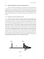
Now, if a coil is wrapped around the sample as in Figure 4, an oscillating voltage
will be induced in the coil by the oscillating magnetization in the sample. This oscillatory
behavior occurs only when M has x or y components. Recall that this is not the case at ther-
sample
rf coil
Figure 4
2/13/01
3. Detection of Precessing Magnetization
9
mal equilibrium. This voltage is generally of the order of microvolts but can be amplified
and recorded. This is the NMR signal.
2/13/01
10
4.
Part I: Lecture Notes
The Rotating Frame.
Consider a coordinate system rotating about the z-axis of a laboratory fixed frame
at an angular frequency, ω. The rotating (primed) coordinate system is then related to the
laboratory fixed system by the transformation:
x ′ = x cos(ωt ) + y sin(ωt )
y ′ = − x sin(ωt ) + y cos(ωt )
(10)
z′ = z
Problem 5: Show that under this transformation the equation of motion for the bulk magnetization becomes
d M′
= γ M′ × Beff
dt
(
)
(11)
where
ω
Beff = B′ −   k ′
γ 
(12)
Thus, in the rotating frame, the equation has the same form as in the laboratory
frame, except that the z component of the external field is reduced by a factor, ω γ . (This
factor is often called the fictitious field.) This means that the solutions will have the same
form as in the laboratory frame except that the precession frequency will be the difference
between the Larmor frequency and the rotating frame frequency. In what follows the
primes will not be carried, but it should be assumed that all equations are in a rotating
frame. The rotating frame used should be evident from the context. Figure 5 illustrates
these results for the case where B is along the z-axis; note that, if ω 0 = ω , then Beff = 0
and M is stationary in the rotating frame. This condition is termed resonance. Without
dwelling on the details of the electronics, one can say that an NMR spectrometer has the
capacity to transform the signals from the probe (laboratory frame) to equivalent signals in
a frame rotating at ω rf .
2/13/01
4. The Rotating Frame.
11
z
Bo
ω o= γ Bo
Bo
z'
ω/γ
M
M
Beff
y
x
∆ω = ω −oω
Laboratory Frame
x'
Figure 5
2/13/01
Rotating Frame
y'
12
Part I: Lecture Notes
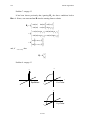
5.
The Effects of Radio Frequency Fields—Pulses.
5.1.
On Resonance Pulses.
Recall that when a sample is placed in a magnetic field, the magnetization goes (after some time) to thermal equilibrium with no transverse components and, consequently,
no NMR signal in the coil. How can one perturb the magnetization away from thermal equilibrium so as to produce transverse components which can be detected?
Using the same coil shown in Figure 5, one can apply an oscillating voltage to the
coil so as to create an oscillating magnetic field in the sample. This oscillating field can be
decomposed into two counter rotating fields. One or the other of these fields will always be
rotating in the same sense as the precession of the nuclear spins. The form of this rotating
field is
[ ( )
( )]
B1 = B1 cos ω rf t i + sin ω rf t j
(13)
Problem 6: Show that the sum of two counter rotating fields is an
oscillating field.
If all three of the frequencies: the oscillating field, ω rf ; the rotating frame, ω; and
the Larmor frequency, ω 0 ; are made equal, then the equation of motion has the form
dM
= γM × B1
dt
(14)
Problem 7: Convince yourself that Equation (14) follows from
those given previously.
This equation says that the magnetization will precess about the direction of the rf
field at a rate ω1 = γB1 . A typical value of ν1 might be 25 KHz. This means that a complete
rotation of the magnetization through 360 degrees would take 40 µs. Suppose, however,
that we turn on the rf transmitter for only 10 µs, delivering a pulse of energy to the sample
which precesses the magnetization through 90 degrees and leaves it in the xy plane. As
shown in Figure 6, by controlling the duration and phase (the phase controls the orientation
of B1 with respect to the rotating frame axes) of the rf pulse the magnetization can be
placed anywhere one desires.
2/13/01
5. The Effects of Radio Frequency Fields—Pulses.
13
Problem 8: Make a figure similar to Figure 6 showing how the
magnetization could be placed along the +x or -y-axes.
5.2.
Off Resonance Pulses.
If ω 0 ≠ ω , then Beff has a component in the z direction because the fictitious field
from the rotating frame transformation does not perfectly cancel B0 . As shown in
Figure 7, Beff is the sum of B1 and this “off resonance” field. The magnetization then precesses about Beff and not about B1 . The magnetization traverses the surface of a cone with
Beff as its axis.
Problem 9: If Beff differs appreciably from B1 , it is not possible
to produce an accurate 180 degree pulse. Explain why and calculate the
magnitude of the error for the best approximation to a 180 degree pulse.
Problem 10: If ω 0 ≠ ω rf , will the time necessary to produce, as
nearly as possible, a 180 degree pulse be longer or shorter than when
z
z
M
Equilibrium
90 x Pulse
M
y
x
B1
x
z
z
180 x Pulse
90 y Pulse
B1
x
M
Figure 6
2/13/01
M
B1
y
x
y
y
14
Part I: Lecture Notes
z
Bo
z
ω/γ
M
B eff
B eff
B1
y
x
y
x
M
Best 180?
Figure 7
ω 0 = ω rf ? Why? Will the phase of the magnetization for a 90 degree pulse
be the same as for an on resonance pulse? In terms of these concepts explain
why carbon-13 isn’t perturbed by a pulse applied to protons.
2/13/01
6. Relaxation—Bloch's Equation.
6.
15
Relaxation—Bloch's Equation.
Thus far our equations provide no means for the magnetization, once perturbed, to
return to thermal equilibrium. Since, experimentally, the magnetization is observed to return to thermal equilibrium, one must introduce dissipative terms which will allow this to
happen. Addition of these terms to the previous equation of motion yields the equation of
motion referred to as Bloch's equation.
d Mx
M
= γ (M × B) x − x
dt
T2
d My
dt
= γ (M × B) y −
My
T2
(15)
d Mz
M − M0
= γ (M × B)z − z
dt
T1
In the absence of all external fields but Bo and with ω = ωo, each component of M decays
independently and exponentially to thermal equilibrium. This process is called relaxation.
Problem 11: Show that, under the above stated restrictions, each of
the above equations has a solution of the form
M = A−αt + C
(16)
What are A, C, and α in each case?
The decay of Mx and My is called transverse or spin-spin or T2 relaxation, and that
of Mz is called longitudinal, spin-lattice, or T1 relaxation.
Problem 12: If one now assumes that ω ≠ ωo, what is the form of
Bloch's equation? This is the equation of motion for a Free Induction Decay
(FID). Recall that Equation (8) deals with this case in the absence of relaxation.
2/13/01
16
Part I: Lecture Notes
1
0.9
0.8
Memory
0.7
0.6
0.5
0.4
τ0
0.3
0.2
0.1
0
0x100 1x10-12 2x10-12 3x10-12 4x10-12 5x10-12 6x10-12
tau
6.1.
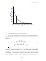
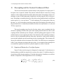
Correlation Functions and Spectral Densities.
The rotational correlation time is a measure of how fast a molecule is tumbling in a
liquid. The spin-lattice and spin-spin relaxation times are related to the rotational correlation time by
(
)
τ0
1
= γ 2 Bx2 + By2
T1
1 + ω 02τ 02
(
)

τ0 
1
1
= γ 2  Bz2τ 0 + Bx2 + By2

2
T2
1 + ω 02τ 02 

(17)
where Bq2 , q = x, y, z is the average of the square of the strength of a random field acting on
a nucleus, ω 0 is the Larmor frequency, and τ 0 is the correlation time of the molecular
tumbling. This correlation time gives a measure of the time required for the molecule to
lose its memory of rotational position as shown in Figure 8. This is called a correlation
function. The Fourier transform of a correlation function is called a spectral density func-
2/13/01
6. Relaxation—Bloch's Equation.
17
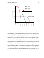
3
tauc = 10^-14
tauc = 10^-12
2.5
Spectral Density
tauc = 10^-10
2
Longer Correlation Time
1.5
Shorter Correlati
1
0.5
1x1016
1x1015
1x1014
1x1013
1x1012
1x1011
1x1010
1x109
1x108
0
Frequency
tion. The amplitude of a spectral density function at a certain frequency controls the relaxation rate. Figure 9 shows examples of spectral density functions for several different
correlation times. The area under each spectral density curve is the same. Figure 10 shows
relaxation times as a function of correlation time. Note how the spin-lattice rate reaches a
maximum then declines while the spin-spin rate continues to increase. Thus, small molecules in nonviscous media show long relaxation times and narrow lines because they are
tumbling rapidly. This is called motional narrowing or extreme narrowing. Note also that
T1 = T2 in this region. By contrast, large molecules, viscous media, or solids are characterized by long spin-lattice relaxation times, but wide lines because the spin-spin relaxation
times are growing ever shorter. Actually, the spin-spin relaxation rate reaches a limit when
all molecular tumbling stops, as in many crystalline solids at low temperature. This effect
is not shown in the figure. The maximum of the spin-lattice curve occurs when ω 0τ 0 = 1 .
This means that when the field strength of a spectrometer is increased, the correlation time
2/13/01
Part I: Lecture Notes
1x100
1x10-1
1x10-2
1x10-3
1x10-4
1x10-5
1x10-6
1x10-7
1x10-8
1x10-9
1x10-10
1x10-11
1x10-12
1x10-13
1x10-14
1x10-15
1x10-16
1x10-17
1x10-18
R1
1
T2
R2
Motional
Narrowing
Limit
1
T1
1x10-18
1x10-17
1x10-16
1x10-15
1x10-14
1x10-13
1x10-12
1x10-11
1x10-10
1x10-9
1x10-8
1x10-7
1x10-6
1x10-5
1x10-4
1x10-3
1x10-2
1x10-1
1x100
R1 = 1/T1, R2 = 1/T2 (1 /sec.)
18
Corr. Time (sec.)
corresponding to the maximum will decrease, but the motional narrowing limit will remain
the same.
6.2.
Relaxation Mechanisms.
Any process that causes the magnetic field seen by the nucleus to fluctuate randomly can cause relaxation.
The following are the most important relaxation mechanisms for high resolution
NMR of liquids. They are arranged roughly in order of decreasing importance for organic
molecules.
6.2.1.
Dipole-Dipole Interactions.
Every other magnetic nucleus in a sample will create a magnetic field at a nucleus
of interest. The nuclei can be in the same or different molecules. The strength of the interaction is inversely proportional to the sixth power of the distance between the nuclei; thus,
2/13/01
6. Relaxation—Bloch's Equation.
19
the nuclei must be very near each other (within a few Angstroms) for a significant interaction to occur. The modulation is caused by rotation and translation of the nuclei.
This interaction can be exploited to measure distances between nuclei.
6.2.2.
Chemical Shift Anisotropy.
We measure chemical shifts as the position of lines in a spectrum relative to some
standard like TMS. Actually the chemical shift depends on the orientation of a molecule
with respect to the external field. In liquids the molecules tumble rapidly with no preferred
orientation, so that the chemical shift we measure is an average of that for all possible orientations of the molecule. However, modulation of the chemical shift as the molecule tumbles produces relaxation. The strength of this interaction is proportional to the square of the
external field. For a 300 MHz or lower spectrometer this effect is usually negligible, but at
500 MHz and above it can be significant.
6.2.3.
Paramagnetic Interactions.
Since the electron has a spin and its magnetic moment is about 2000 times greater
than that of nuclei, dipole-dipole interactions of nuclei with electrons can be a dominant
relaxation mechanism. Fortunately, most electrons come in pairs of opposite spin and cancel each other out. Molecules or ions with unpaired electrons are called paramagnetic. Free
radicals, and metal ions of iron or chromium are examples. If such species are present in a
NMR sample, even in very low concentration, T2 relaxation may be so rapid that nuclear
spin signals are very broad and cannot be resolved from each other. Molecular oxygen is
mildly paramagnetic, so dissolved oxygen does contribute to relaxation.
6.2.4.
Spin-Rotation Interactions.
For small molecules rotating rapidly and undergoing collisions with other molecules, interaction of the magnetic field produced as the molecule rotates with the nuclear
magnetic moment can produce relaxation. For most organic molecules this effect is negligible. Dissolved CO2 would be an example where it would be non-negligible. This mechanism becomes more important as the temperature is increased in contrast to other
mechanisms which vary inversely with temperature.
2/13/01
20
6.2.5.
Part I: Lecture Notes
Quadrupolar Interactions.
If a nucleus has a quadrupole moment, deuterium for example, and is in an unsymmetrical electronic environment, this can produce a fluctuating field that causes relaxation.
Since carbon-13 and protium have no quadrupole moment, this mechanism is often unimportant for structural organic chemistry.
6.2.6.
Scalar Interactions.
Just as for dipole-dipole and quadrupolar interactions, scalar interactions or J-couplings depend on molecular orientation and the values we see in liquid spectra are averages
over all orientations. Likewise, the modulations involved can produce relaxation. However,
this effect is usually negligible in organic molecules.
2/13/01
7. The CW NMR Experiment.
7.
21
The CW NMR Experiment.
Now suppose one turns on a B1 field along the x direction of the rotating frame. The
equation of motion becomes
d Mx
M
= γ My ∆B − x
dt
T2
M
d My
= − γ Mx ∆B + γ Mz B1 − y
dt
T2
(18)
d Mz
M − Mo
= − γ My B1 − z
dt
T1
where
∆B =
ω − ωo
γ
Problem 13: If B1 is small show that the steady state solution of
these equations is
Mx = χ oω o T2
(ω − ω o )T2 B
2
1
1 + (ω − ω o ) T2 2
My = χ oω o T2
1
B1
2
1 + (ω − ω o ) T2 2
(19)
Mz = Mo
where
χo =
Mo
Bo
Suppose one keeps Bo and B1 constant and changes ω slowly. Then the NMR signal
has the form
Fx (ω ) = AT2
(ω − ω o )T2 B
2
1
1 + (ω − ω o ) T2 2
1
Fy (ω ) = AT2
B1
2
1 + (ω − ω o ) T2 2
2/13/01
(20)
22
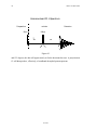
Part I: Lecture Notes
Absorption
Dispersion
+
0
Frequency
-
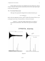
Figure 11
where A represents various constants including the efficiency with which one can detect
and amplify the voltage induced in the receiver coil. This equation represents the basic continuous wave (cw) NMR experiment. Figure 11 shows the form of these two signals. Fx
represents what is termed the dispersion mode signal, while Fy is the absorption mode. The
latter is the signal usually displayed when one records a cw spectrum.
Problem 14: Make a scaled plot similar to Figure 11. What is the
effect on the curves of changing B1 or T2? What is the full width at half maximum (fwhm) of the absorption curve? How many fwhm units does it take
for the absorption mode to fall to one percent of its maximum value? How
many for the dispersion signal?
2/13/01
8. The FT NMR Experiment.
8.
23
The FT NMR Experiment.
If one applies a 90 degree pulse along the x-axis, the magnetization is left along the
y-axis. The magnetization as a function of time, subsequent to the pulse, has the form
[
)
cos[(ω
M x = M0 e
− ( t T2 )
M y = M0 e
− ( t T2
]
− ω )t ]
sin (ω 0 − ω )t
0
(21)
The NMR signal (FID) detected by the spectrometer is, of course, proportional to this magnetization (see Figure 12). It is convenient to define a complex FID as
f (t ) = My + iMx
(22)
My
t2
Mx
Figure 12
2/13/01
24
Part I: Lecture Notes
A Fourier transform (FT) is then performed on this FID according to
F (ω ) = ∫
∞
−∞
f (t )e −iωt
(23)
resulting in
F (ω ) =

M0 T2 
1
ω − ω0
2 2 +i
2 2

2  1 + (ω − ω 0 ) T2
1 + (ω − ω 0 ) T2 
(24)
Comparing Equation (24)with the results of the cw experiment, Equation (20), the real part
of F(ω) corresponds to the absorption mode signal and the imaginary part to the dispersion
mode. Figure 12 shows a complex FID and the corresponding FT spectrum is identical to
that shown in Figure 11.
Problem 15: What would be the difference between a FID from a
resonance above the rotating frame in frequency as opposed to one whose
frequency is less than that of the rotating frame by the same amount?
If one has a spectrum with many lines, a pulse may be applied to simultaneously
excite all of the lines and a FID collected containing the spectral information from all the
resonances. A Fourier transform can then be performed to produce a spectrum containing
all the information that, by cw methods, would require slowly sweeping through each resonance and recording the result.
2/13/01
9. The Anatomy of a Free Induction Decay.
9.
25
The Anatomy of a Free Induction Decay.
Intelligent operation of an NMR spectrometer requires a clear understanding of the
FID and its relationships to the transformed spectrum. Since all processing of the FID is
done using a digital computer, it is also important to understand the consequences of converting the FID to digital form.
9.1.
FID of a Single Resonance.
Figure 12 shows the complex FID of a single resonance such as might be obtained
from a sample of chloroform and Figure 11 shows the Lorentzian line which would be obtained from Fourier transforming this FID. They have the following properties:
a.
The initial amplitude of the FID is proportional to the height or the
integrated intensity of the line.
b.
The time constant, T2* of the exponential decay of the FID is related
to the full width at half maximum, L, of the absorption mode signal
by
L=
1
πT2*
(25)
Thus, FID's with short time constants give wide lines and FID's with
long time constants give narrow lines.
9.2.
c.
The frequency of the oscillation is ∆ω, the frequency difference between the transmitter and the line.
d.
The phase of Mx indicates the sign of the frequency. If counterclockwise rotation (as viewed from the positive z-axis) is taken to be
positive, then the FID as shown represents a negative frequency. If
the phase of Mx is shifted by 180 degrees, then the frequency would
be positive.
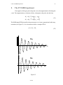
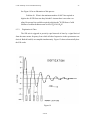
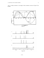
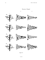
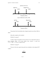
FID of Two or More Lines.
The FID of two or more lines is obtained by summing the FID's corresponding to
the individual lines. As shown in Figure 13 (a), two lines give a fairly simple FID. In this
case the two lines have frequencies of 20 and 25 Hz. The frequency associated with the interference beats gives the separation of the two lines, 5 Hz in this case. However, as one
adds more lines to the FID, it quickly becomes too complicated to analyze visually.
2/13/01
26
Part I: Lecture Notes
2
Amplitude
(a)
1
0
-1
-2
0
0.2
0.4
0.6
Time (sec)
0.8
1
4
Amplitude
(b)
2
0
-2
-4
0
0.2
0.4
0.6
Time (sec)
0.8
1
Figure 13 (b) shows a FID with four lines. Lines at 7 and 63 Hz have been added to the FID
of (a).
9.3.
9.3.1.
Digitization of Free Induction Decays.
Digitization in Amplitude.
The FID is sampled by the sample and hold unit (S/H), converted to digital form by
the analog to digital converter (ADC), and stored in the computer memory.
The dynamic range of the digitized FID and, consequently, of the spectrum depends
on the number of bits in the ADC.
Noise can be introduced due to truncation errors.
2/13/01
9. The Anatomy of a Free Induction Decay.
27
See Figure 14 for an illustration of this process.
Problem 16: What is the minimum number of ADC bits required to
digitize the 1H FID from tert-butyl alcohol? Assume there is no scalar coupling. How many bits would be required to digitize the 1H FID from a 5 mM
solution of sodium dichloroacetate in 90% H2O/10% D2O?
9.3.2.
Digitization in Time.
The S/H unit is triggered at precisely equal intervals of time by a signal derived
from the same master frequency from which all other frequencies in the spectrometer are
derived. Both Mx and My are sampled simultaneously. Figure 15 shows schematically how
the S/H works.
Figure 14
2/13/01
28
Part I: Lecture Notes
The spectral width, S, over which resonances can be accurately sampled is given by
S=
N
A
(26)
where N is the number of complex samples of the FID (The number of points parameter on
most spectrometers is 2N, counting one for the real and one for the imaginary part of
the FID.) and A is the total time during which the FID is sampled, the acquisition time. The
spectral width encompasses the range ±S/2 from the frequency of the transmitter.
The interval between data points in the FID will be A N = 1 S and the separation
in the spectrum will be S N = 1 A .
Amplitude
Problem 17: Assuming that two adjacent lines are narrower than
1/A, how close to each other can they be and still be detected as separate
lines? Suppose that this separation were due to a scalar coupling; what error
limits should you report for the coupling constant?
A/N
2A/N
Time
Figure 15
2/13/01
3A/N
4A/N
9. The Anatomy of a Free Induction Decay.
29
If the computer memory is capable of accommodating only Nmax complex data
points, then the product of S and A cannot exceed this value.
Problem 18: Find out what the value of Nmax is for the spectrometer
you are using and compute the best resolution you can obtain using a spectral width sufficient to cover the nominal maximum chemical shift range for
1H.
Do the same for 13C. If you have shimmed the magnet to 0.2 Hz line
width, what is the maximum spectral width you can use while retaining your
hard won resolution?
Resonances which occur outside the spectral width defined by the sampling rate are
aliased to a point within the spectral width as shown in Figure 16. This phenomenon is often incorrectly referred to as foldover rather than aliasing.
If only the real or only the imaginary part of the FID is acquired, the ability to discriminate between signals above and below the transmitter in frequency is lost, and each
line will appear on both sides of the carrier and equidistant from it. One will be a phantom
image and the other the real line. One cannot distinguish between the two without additional information. This phenomenon is correctly termed foldover because it is as though the
spectrum were folded about the transmitter frequency and the two halves superimposed.
Problem 19: If the transmitter is moved a small amount or the spectral width is changed by a small amount, how will images, real lines, and
aliased lines respond? How can this information be used to detect the false
lines?
9.4.
Time Averaging.
Suppose one acquires N identical FID's. Each sample of each FID contains a signal
component, S, and a noise component which will be supposed to be random (Gaussian distributed) with standard deviation σS. Then, if one adds the FID's, the signal components
will add coherently to give a total signal, St , according to
St = NS
2/13/01
(27)
30
Part I: Lecture Notes
My
Mx
0.0 0.1 0.2 0.3 0.4 0.5 0.6 0.7 0.8 0.9 1.0
Time (ms)
Real Line
Aliased Line
-SW/2
-10
-5
SW/2
0
Frequency (KHz)
Figure 16
2/13/01
5
10
9. The Anatomy of a Free Induction Decay.
31
But it can be shown that σt, the standard deviation of the noise in the time averaged FID, is
given by
σ t = Nσ S
(28)
Hence, taking the ratio of the signal to the noise in the summed FID
St =
St
=
σt
NS
S
= N
Nσ S
σS
(29)
Thus, the signal to noise ratio St of a time averaged FID increases as the square root of the
number of FID's averaged.
Problem 20: After running a sample all day (say 12 hours) you are
beginning to see what you think are signals (signal to noise ratio about 2).
How much longer will it take to get a publishable spectrum (signal to noise
ratio about 10)?
The fact that one is time averaging digitized FID's also has some consequences of
which one needs to take account when planning experiments. Time averaging cannot produce a FID with signal to noise ratio greater than the dynamic range of the computer memory cell into which it is being time averaged. When the largest value in a time averaged FID
overflows the computer memory cell being used to store it, the data must be scaled in order
to continue time averaging; but, for each factor of two by which the data is scaled, one bit
of the ADC becomes useless decreasing the effective dynamic range of the ADC by a factor
of two. When this process reaches a point where the least significant effective bit of the
ADC represents a value larger than the noise level, no amount of additional time averaging
can bring additional small signals out of the noise.
In Section 6 we learned about T1 relaxation. Let us examine what effect longitudinal relaxation has on time averaging of FID’s. Suppose we apply a θ degree pulse to a spin
system every t seconds, collect a FID after each pulse, and time average N such FID’s in a
total time of To = Nt . Starting from thermal equilibrium, the amplitude of the first FID will
be proportional to Mo sin θ , but, if t is short enough so that the magnetization does not fully
relax, the magnetization available to generate the second FID will be smaller and for the
2/13/01
32
Part I: Lecture Notes
third FID still smaller and so on. A steady state will be reached after a few pulses characterized by Equation (30).
M + = M − cosθ
(
)
M − = Mo + M + − Mo e − r
(30)
where
M + = the z axis magnetization just after the pulse
M − = the z axis magnetization just before the pulse
Mo = the thermal equilibrium magnetization
r = t T1
Substituting the first line of Equation (30) into the second and solving for M − gives
Equation (31).
er − 1
M = Mo r
e − cosθ
−
(31)
The xy magnetization following the pulse is M − sin θ , and the amplitude of the FID is proportional to this quantity. Hence, the signal amplitude for each FID can be rewritten for this
case as Equation (32).
S(θ , r ) = KM − sin θ = KMo sin θ
er − 1
e r − cosθ
(32)
Then, we know from Equation (29) that the signal-to-noise after N FID’s is proportional to
N . Hence, we can write Equation (33).
St (θ , r ) =
N
KMo N
er − 1
S(θ , r ) =
sin θ r
σS
σS
e − cosθ
2/13/01
(33)
9. The Anatomy of a Free Induction Decay.
33
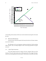
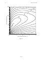
However, the interesting question is: What values of θ and r will give maximum signal-tonoise per unit time? To answer this we write Equation (34).
St′(θ , r ) =
St (θ , r ) KMo N
er − 1
=
sin θ r
σ S To
To
e − cosθ
KMo
er − 1
=
sin θ
σ S ToT1
re r − cosθ
= K ′ sin θ
(34)
er − 1
re r − cosθ
The explicit dependence on N has been eliminated by using the fact that
N=
To To
=
t
T1r
and all of the constants have been absorbed into a new constant by defining
K′ =
KMo
σ S ToT1
Equation (34) tells us how signal-to-noise per unit time depends on the values of θ and r.
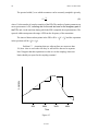
Figure 17 shows a contour plot of this equation. Note that 90 degree pulses never give maximum signal-to-noise per unit time regardless of the repetition rate.
2/13/01
34
Part I: Lecture Notes
150
0.50
0.60
0.70
.80
Tip Angle (degrees)
100
0.90
0.99
50
0
0
1
2
Pulse Repetition Rate t/T1
Figure 17
2/13/01
3
4
10. Digital Filters and Convolution.
35
10. Digital Filters and Convolution.
In the context of NMR spectroscopy digital filters are computational algorithms that
reject unwanted signals or noise and allow desirable signals to pass through to the final
spectral display. Filters can also alter line shapes with either desirable or undesirable results. These undesirable results are generally caused by unintentional digital filtering.
10.1. The Convolution Theorem.
In preparation for discussion of digital filters it is necessary to understand the Fourier convolution theorem. Suppose one has three functions of time, a(t), b(t), and c(t), such
that,
c ( t ) = a ( t )b ( t )
(35)
then, if A(ω), B(ω), and C(ω), are the Fourier transforms of each of the corresponding time functions, it can be shown that
∞
C(ω ) = ∫ d ω ′ A(ω ) B(ω − ω ′ )
−∞
(36)
Of course, these computations must be done on sampled functions as has been discussed
previously. Figure 18 illustrates how the convolution operation works in the frequency domain for two lines of equal width. In the computer the calculation would actually be done
by multiplying the FID's corresponding to the two lines together and transforming the product to give the convolved spectrum. Due to the computational efficiency of the FFT, this
can be done far faster than computing the convolution directly. The former takes only
2Nlog2N operations, whereas, the latter requires N2 operations. This increase in computational efficiency is the power of the convolution theorem.
Problem 21: Compute the increased computational efficiency of the
FFT method over direct computation for convolution of two 1K (1024)
point data tables and for two 32K (32,768) point data tables.
2/13/01
36
Part I: Lecture Notes
Figure 18
2/13/01
10. Digital Filters and Convolution.
37
10.2. Deconvolution.
If a spectrum has been convolved with some particular function, (perhaps due to an
artifact of the instrumentation, such as, magnet inhomogeneity) it is possible to conceive of
undoing the process by writing
a( t ) =
c( t )
b( t )
(37)
This is, indeed, possible; however, certain limitations apply since one must avoid dividing
by zero; and, of course, it is impossible to recover data lost because the original c(t) was
zero over some particular interval.
10.3. Truncation of the FID.
If one stops taking data before the FID has completely died away into the noise, this
can be viewed as convolution. The FID has been multiplied by a function of the form
0 t < 0

f (t ) = 1 0 ≤ t ≤ A
0 t > A

(38)
where A is the spectrometer acquisition time. This corresponds to convolving the spectrum
with a (sin x)/x function. (See Figure 19.) The (sin x)/x function is the Fourier transform of
the rectangular function Equation (38).
10.4. Apodization.
The effects of this undesirable convolution can be alleviated by a technique called
apodization. This consists of smoothing the tail of the FID so as to eliminate the sharp edge
produced by the rectangle function. Almost any smooth function will produce desirable effects; one method is shown in Figure 19.
10.5. Sensitivity Enhancement.
An FID can be written in the form
f (t ) = exp( −iω t − t T2 )
2/13/01
(39)
38
Part I: Lecture Notes
Recall that the width of the line when one Fourier transforms this function is given by
Equation (25). Suppose the above function is multiplied by one of the form
fc (t ) = exp( − t TLB )
(40)
Problem 22: Show that the complex exponential form of the FID
Equation (39) is just another way of writing Equation (22). Show that multiplying Equation (39) by Equation (40) gives, in the spectrum, a Lorentzian
line with frequency, ω, and width,
L=
1
1
+
πT2 πTLB
corresponding to the convolution of the two Lorentzians.
Figure 19
2/13/01
(41)
10. Digital Filters and Convolution.
39
The line width is increased by 1/πTLB which decreases the resolution, but, as shown
in Figure 20, the noise in the spectrum is substantially decreased, thus, improving the signal
to noise ratio of the spectrum.
10.6. Resolution Enhancement.
If the sign of the exponential is changed in the convolution function to give
fc (t ) = exp( + t TLB )
(42)
then, by the same arguments given above, the line width will be decreased. However, just
as the signal to noise ratio was increased before, it will now be decreased.
Problem 23: Show that resolution enhancement is an example of
deconvolution as defined above. Hint: What is the reciprocal of an exponential?
Figure 20
2/13/01
40
Part I: Lecture Notes
10.7. Lorentzian to Gaussian Transformation.
Consider a convolution function of the form
fc (t ) = exp( + t TLB − t 2 TG2 )
(43)
This corresponds to simultaneous convolution with a Gaussian and deconvolution with a
Lorentzian. In an ideal situation this will convert a Lorentzian line into a Gaussian line.
This is a technique commonly used in 2D NMR.
2/13/01
11. Decoupling and the Nuclear Overhauser Effect.
41
11. Decoupling and the Nuclear Overhauser Effect.
Thus far our discussion has centered mainly on the properties of a single spin-1/2,
but spins are not, in general, isolated. They interact with each other in various ways, among
which are scalar coupling and nuclear dipole-dipole interactions. Decoupling consists of irradiating a system of interacting spins continuously and observing the effect on the spectrum. Decoupling is termed heteronuclear if the observed and irradiated nuclei are different
nuclear species, e.g., one can observe 13C while irradiating 1H; or homonuclear if they are
the same, e.g., one can irradiate a particular proton while observing the effect on the rest of
the proton spectrum. A commonly used notation for these two experiments is 13C{1H} and
1H{1H} respectively.
The term decoupling stems from the fact that, when a spin is irradiated, the fine
structure or splittings of all the other spins in the coupling network which are due to scalar
coupling with the irradiated spin are collapsed, so that the splitting pattern appears as if the
irradiated spin were not coupled to the others. The intensities of the remaining resonances,
however, may be substantially different from those expected in a spin system created by
removing the irradiated spin and considering only the remaining spins. These intensity differences are called the nuclear Overhauser effect (NOE). The NOE arises as a consequence
of the T1 type relaxation occurring in the spin system. As an example of these principles let
us examine the equation of motion for a proton coupled to a carbon-13 nucleus.
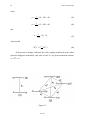
11.1. Equation of Motion for a Two Spin System.
Figure 21 shows (a) the energy level diagram of a single spin-1/2 with only one relaxation pathway available in contrast to (b) a system of two spins-1/2 with four energy levels and six possible relaxation pathways. Using the density matrix formalism, one can show
that the z-components of the magnetization evolve according to
C
 ρC
d  Mz (t ) 
=
−

σ
d t  MzH (t )
σ   MzC (t ) − MzC (∞) 

ρ H   MzH (t ) − MzH (∞)
2/13/01
(44)
42
Part I: Lecture Notes
where
ρC =
1
= W2 + 2W1C + W0
T1C
(45)
ρH =
1
= W2 + 2W1H + W0
T1H
(46)
1
= W2 − W0
T1CH
(47)
and
σ=
Also note that
MzH (∞) =
γH C
Mz ( ∞ )
γC
(48)
If the proton is strongly irradiated, the scalar coupling manifested in the carbon
spectrum disappears immediately; and, after several T1's, the proton transitions saturate,
i.e., MzH → 0 .
Figure 21
2/13/01
11. Decoupling and the Nuclear Overhauser Effect.
43
Problem 24: Show that under decoupling the steady state solution
of the equation of motion is
(
)
(49)
γ Hσ
γ C ρC
(50)
MzC = 1 + ηC{H} MzC (∞)
where
ηC{H} =
Under proton decoupling the equation of motion for the 13C magnetization becomes
[
]
d MzC (t )
= −ρC MzC (t ) − 1 + ηC{H} MzC (∞)
dt
(
)
(51)
This means that the 13C magnetization evolves just as though the proton is not there except
that it evolves toward the NOE enhanced value rather than toward the usual thermal equilibrium. If the relaxation is purely dipolar, then ρC = 2σ , and η = 2.Thus, the carbon magnetization will be enhanced by a factor of 1 + η = 3. If other relaxation mechanisms are
important, the factor will be less than three. It is the factor, 1 + η, which is generally referred to as the NOE.
The same principles apply to other nuclear pairs besides protons and carbon-13; but
note that, if the gyromagnetic factors have opposite sign as would be the case for protons
and nitrogen-15, then the NOE would be negative, and line intensities would be decreased
from their thermal equilibrium values even becoming zero or negative.
Problem 25: What would be the NOE for a 15N{1H} experiment under purely dipolar relaxation? Draw a schematic 15N spectrum of formamide showing intensities to scale with and without proton decoupling.
Ignore the long-range coupling to the formyl proton.
11.2. Homonuclear Decoupling.
The discussion above applies equally well to a system of two nonequivalent protons.
Problem 26: What would the maximum NOE be for two protons?
2/13/01
44
Part I: Lecture Notes
Since the dipolar relaxation mechanism depends critically on the through space distance between the interacting nuclei, it is possible in certain cases to determine internuclear
distances using proton-proton NOE's. This technique is coming to be widely used for determining structure in macromolecules such as proteins.
11.3. Broadband Decoupling.
The usual way to run 13C spectra is with all the protons decoupled. To accomplish
this it is, in general, necessary to simultaneously irradiate protons of varying chemical
shifts. This is done by modulating the decoupler rf transmitter so as to spread the power
over the necessary band of frequencies. For a number of years this was done by using pseudo random noise for modulation, but more recently other techniques have been developed
which use the available power more effectively. The current best such technique for
13C{1H} experiments seems to be the WALTZ modulation sequence of Freeman. It is important to minimize the amount of power used for broadband decoupling. Since the power
is on continuously, it can heat the sample in much the same way as a microwave oven heats
food. Using WALTZ modulation it is generally possible to decouple over the full proton
chemical shift range using power levels of the order of one watt in a five or ten millimeter
sample.
2/13/01
12. Multiple Pulse Experiments, Spin Echoes, Measurement of T1 and T2.
45
12. Multiple Pulse Experiments, Spin Echoes, Measurement of T1 and T2.
In the preceding section the consequences of subjecting the nuclear spins to a single
radio frequency pulse were outlined, but the great variety of data available from NMR experiments is obtained principally from subjecting the spins to multiple pulses of various
phases and amplitudes separated by carefully chosen delays. Many of the principles involved can be illustrated using a simple two pulse sequence to measure the value of T1 and
T2 .
12.1. Measurement of T1 by Inversion Recovery.
We have seen previously, Equation (16), how the z component of the magnetization
relaxes exponentially back to thermal equilibrium whenever it is disturbed from that state.
Figure 22 shows a pulse sequence which permits quantitative measurement of this process
by producing a series of partially relaxed spectra. By varying the time t1 between the 90
and 180 degree pulses the partially relaxed z magnetization is projected on the y-axis. Fourier transformation of the resulting FID and measurement of the peak intensities then produces a set of data for each peak in the spectrum which can be analyzed to obtain the value
of T1. (See Equation (55).)
Problem 27: We have considered previously (Figure 7) the inadequacy of a 180 degree pulse when Beff differs appreciably from B1, i.e.,
when the line is too far off resonance. If the 180 degree pulse is replaced by
90(x)
180(x)
t1
t2
Figure 22
2/13/01
46
Part I: Lecture Notes
a “pulse sandwich” of the form 90(x)180(y)90(x), describe how this situation will be improved.
12.2. Hahn Spin Echoes.
Figure 23 shows another pulse sequence which permits the measurement of T2. At
2τ, dephasing due to magnet inhomogeneity is reversed and the magnetization in said to
refocus or form a spin echo. The concept of refocussing of magnetization is critical to an
understanding of two dimensional experiments. True T2 processes, which are stochastic or
random in nature, do not refocus; so the amplitude of the magnetization is reduced but only
by these stochastic processes. The second half of the echo can be Fourier transformed to
produce a spectrum in the usual way. The value of T2 can be extracted from peak intensities
measured from a series of such spectra taken as a function of t1 in much the same way as
was described for the T1 measurement.
12.3. Measurement of T2 by the Carr, Purcell, Meiboom, Gill Method.
If the spins diffuse into a region of different magnetic field during t1, this constitutes
a stochastic process; then the refocussing will not accurately represent spin-spin relaxation
processes. This problem can be largely overcome by the pulse sequence of Figure 24. The
series of 180(y) pulses repeatedly refocuses the magnetization. In this case only the diffusion happening during 2τ effectively reduces the echo amplitude. By making τ short
enough, the effects of diffusion can be made insignificant. The second half of each echo
can be taken as an FID, Fourier transformed, and analyzed as before. With the pulse se-
90(x)
180(y)
τ
τ
t2
t 1 = 2τ
Figure 23
2/13/01
12. Multiple Pulse Experiments, Spin Echoes, Measurement of T1 and T2.
0(x)
[
47
80(y)
τ
τ
]n
t2
t = 2nτ
Figure 24
quence as written in Figure 24, pulse imperfections in the 180 degree pulses tend to accumulate. But, merely by alternating the phase of successive y pulses this can largely be
eliminated.
Problem 28: This experiment will work also if the train of 180 degree pulses is not phase shifted with respect to the initial 90 degree pulse.
How will the results of the experiment differ in this case? Why is this not a
better way to measure T2?
2/13/01
48
Part I: Lecture Notes
13. Polarization Transfer, INEPT and DEPT.
The magnetization generated in a sample depends on the γ of the nucleus involved,
so a high γ nucleus, such as 1H, develops greater magnetization in a constant field than, for
example, 15N or 13C. If a high γ nucleus and a low γ nucleus are coupled by scalar coupling,
magnetization can be transferred from the high to the low γ nucleus thus increasing the sensitivity with which the low γ nucleus can be detected.
13.1. INEPT.
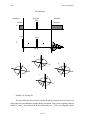
Figure 25 shows the pulse sequence used for the INEPT (Insensitive Nucleus Enhanced by Polarization Transfer) experiment. Vector diagrams show the evolution of the
magnetization at key points. The principle problem with this method is that antiphase multiplets are generated which cancel to produce zero intensity when decoupling is applied. An
additional refocussing step can be added to the pulse sequence to overcome this problem,
but the DEPT pulse sequence also solves this problem and has other positive attributes as
well.
13.2. DEPT.
Figure 26 shows the DEPT (Distortionless Enhancement by Polarization Transfer)
pulse sequence and vector diagram. Since DEPT depends on the properties of double quantum coherence to achieve its effect, the vector diagrams are not completely satisfactory, but
do provide some sense of what is happening to the magnetization. Scalar coupled multiplets
produced by DEPT are enhanced but have the same intensity ratios as a normal FT spectrum. Thus, they can be easily interpreted or decoupled to produce a simpler spectrum in
the usual way. By adjusting the width, θ, of the final proton pulse, one can produce spectra
which identify various types of spin systems. Figure 27 shows how CH, CH2, and CH3 spin
systems respond to the tip angle of the final proton pulse with all other parameters of the
pulse sequence kept constant. For θ = 90degrees only methine carbons appear in the spectrum. For θ = 135 degrees methine and methyl carbons are positive while methylene carbons are negative. Of course, quaternary carbons never appear because there is no source
of polarization for them. These two spectra plus an ordinary proton decoupled FT spectrum
to pick up the quaternary carbons provide sufficient information to determine the number
of directly bonded protons for each carbon in the spectrum. One additional DEPT spectrum
with θ = 45 degrees yields three independent pieces of information, so that appropriate linear combinations of the three spectra can yield subspectra containing only methine, meth-
2/13/01
13. Polarization Transfer, INEPT and DEPT.
49
z
b
z
d
y
y
x
x
z
a
z
c
z
e
y
y
y
x
x
x
INEPT
90(x)
1
H
180(x)
1/4J
a
90(y)
1/4J
b
d
c
180(x)
e
90(x)
13
C
t2
f
z
f
y
x
Figure 25
2/13/01
50
Part I: Lecture Notes
z
z
x
x
z
z
z
a
x
x
0(x)
x
DEPT
θ (y)
180(x)
Decouple
H
1/2J
/2J
/2J
b
e
90(x)
80(x)
3
C
2
h
f
z
z
z
f
x
z
x
x
h
y
x
Figure 26
2/13/01
13. Polarization Transfer, INEPT and DEPT.
51
ylene, or methyl resonances. An example of this treatment is shown in Figure 28 for
menthol.
Figure 27
Figure 28
2/13/01
52
Part I: Lecture Notes
The DEPT experiment can also be used as a convenient method for calibrating the
proton pulse width. Usually, in experiments of this type, proton pulses are applied using the
decoupler transmitter. Since the decoupler pulses, B2, essentially always have a different
calibration factor than the observe pulses, B1, it is necessary to have an indirect method of
calibrating B2 with the instrument set up as it will be when the experiments which will use
the calibration are done. This can be accomplished by observing a methylene resonance using a DEPT pulse sequence with θ set to nominally 90 degrees. Then, adjusting the proton
pulse width, one can observe the methylene resonance to pass through a null as the proton
pulse passes through exactly 90 degrees. If the calibration point is completely unknown, a
rough calibration can be achieved by setting θ to a nominal 45 degree value and searching
for a maximum intensity as a function of the proton pulse width. This calibration can be
used in numerous other one and two dimensional experiments where decoupler pulses are
required.
2/13/01
14. Fundamental Concepts of Two Dimensional NMR.
53
14. Fundamental Concepts of Two Dimensional NMR.
Before discussing specific 2D experiments some fundamental concepts characteristic of all 2D experiments will prove useful.
14.1. The Generic 2D Pulse Sequence.
Four time periods characterize a 2D experiment as shown in Figure 29. Each of the
four periods can take a variety of forms depending on the experiment, but some fairly typical examples can be given. Preparation frequently consists of just waiting long enough for
the spins to be sufficiently close to thermal equilibrium or some steady state condition then,
perhaps, applying a 90 degree pulse to produce transverse magnetization or coherence.
Thus prepared, the magnetization is allowed to evolve, often with some refocussing pulses,
so as to exhibit some desired characteristic of the spin system as a function of t1. The mixing period can be used to enhance certain aspects of the evolving magnetization, i.e., to filter out just the information the experimenter wants and convert it into the single quantum
coherence which can be detected by the spectrometer. During detection the carefully prepared transverse magnetization is sampled as a function of t2. Systematic incrementation of
t1 with sampling of the resulting transverse magnetization as a function of t2 for each t1 increment, yields a two dimensional FID as illustrated in Figure 30. The form of the 2D FID
is


t 
t 
f (t1 ,t2 ) = exp −iω i t1 − 1  exp − jω j t2 − 2 .
T2,1 
T2,2 


Preparation
Evolution
Mixing
(optional)
1
Figure 29
2/13/01
Detection
(52)
Part I: Lecture Notes
Amplitude
54
1
0
0.5
-1
0
0.3
t2
t1
0.2
0.1
0.4
Figure 30
The function f is called hypercomplex because it is complex in both the t1 and t2 dimensions. The imaginary numbers i and j are defined such that i 2 = −1 , and j 2 = −1 , but
ij ≠ −1 . Thus, Equation (52) involves four types of terms: those involving neither i nor j,
those involving i, those involving j, and those involving the product ij. These terms are often referred to as real-real, imaginary-real, real-imaginary, and imaginary-imaginary respectively. Figure 30 shows the real-real part of f. This will be discussed further in
Section 14.3.
14.2. The Two Dimensional Fourier Transform.
The FID must now be subjected to a 2D Fourier transform. First, each of the FID's
is transformed with respect to t2 applying any convolution functions desired. This produces
a matrix which is a function of t1 and ν2 as shown in Figure 31. The time functions
in the t1 domain have the appearance of FID's, but in the literature they are often
called interferograms. Each interferogram is now transformed with respect to t1 after
2/13/01
14. Fundamental Concepts of Two Dimensional NMR.
55
1
Amplitude
0.5
0
-0.5
-1
0.2
0
0.16
2
0.12
4
ν2
0.08
6
8
0.04
10 0
t1
Figure 31
applying any convolution functions. The result is then a two dimensional Lorentzian
line, a function of ν1 and ν2, modified by any convolutions as shown in Figure 32.
14.3. Phase Sensitive 2D NMR.
Figure 32 shows a pure absorption line shape in both dimensions; however, many
2D experiments do not yield this result but rather what is called a phase twist line shape as
shown in Figure 33. This line shape has strong tails and a much wider appearance due to
the dispersion contribution. Figure 31 shows pure amplitude modulation of the ν2 spectra
as a function of t1. This phase twist line shape results from phase modulation as a function
of t1. as shown in Figure 34. Generally the pulse sequences that produce a phase twist line
shape are those that are designed to achieve quadrature detection in the t1 dimension. Spectra with this phase twist line shape are normally displayed as the absolute value of the hy-
2/13/01
56
Part I: Lecture Notes
Amplitude
1
0.5
0
10
0
8
2
ν2
6
4
4
6
8
2
ν1
10 0
Figure 32
percomplex quantities. An alternative method first published by States, Haberkorn, and
Ruben makes use of two data sets to produce a spectrum that can be displayed as a twodimensional pure absorption mode spectrum with lines as in Figure 32. In the time domain
one data set is amplitude modulated like that shown in Figure 30, while the second is similar, but the amplitude modulation with respect to t1 is 90 degrees out of phase as shown in
Figure 35. One then has four data sets or quadrants as mentioned in Section 14.1 which can
be transformed to yield the corresponding hypercomplex spectrum. Phasing of such a spectrum is somewhat more complex than for a one-dimensional spectrum since linear combinations of all four quadrants of the hypercomplex data are required.
2/13/01
14. Fundamental Concepts of Two Dimensional NMR.
57
Amplitude
1
0.5
0
-0.5
10
0
8
2
6
4
ν2
4
6
8
2
ν1
10 0
Figure 33
14.4. Phase Cycling.
Phase cycling is used in both one and two dimensional spectroscopy to cancel
artifacts and unwanted signals while retaining the information which the experimenter wants. The basic idea is to create a series of FID's, such that, the unwanted
coherences alternate in phase while those to be kept have always the same phase.
Thus, when the FID's are added together, the unwanted parts interfere destructively,
but the desired parts interfere constructively. Simultaneously, of course, the signal to noise
improves as we have discussed previously. However, whether or not the signal to noise improvement is needed, some minimum number of FID'S must be acquired to permit the
phase cycle to complete. This number may be as small as two or as large as 1024 or more.
2/13/01
58
Part I: Lecture Notes
1
Amplitude
0.5
0
-0.5
-1
0.2
0
2
0.16
ν2 4
0.12
0.08 t1
6
8
0.04
10 0
Figure 34
The signals to be cancelled out may be thousands of times larger than the desired signals
or they may be much smaller.
14.4.1. Elimination of Detector Asymmetry.
One of the oldest applications of phase cycling eliminates the effects of unequal
gain in the two quadrature channels of the spectrometer. The gains of the two channels in
a spectrometer nearly always differ sufficiently to produce an observable image without
phase cycling. The image appears as a result of foldover of the part of the signal in the higher gain channel which has no compensating signal in quadrature in the lower gain channel.
Consider the consequences of altering the phase of successive pulses in an ordinary onepulse FT experiment as shown in Figure 12 according to: 90x, 90y, 90-x, 90-y. Figure 36
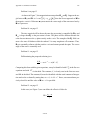
shows the FID's obtained. Table I shows how the FID's can be combined to yield a final
FID nominally the same as that resulting from four 90x pulses. Note, however, that both the
2/13/01
14. Fundamental Concepts of Two Dimensional NMR.
59
1
Amplitude
0.5
0
-0.5
-1
0.2
0
0.16
2
0.12
4
ν2
0.08
6
0.04
8
10 0
t1
Figure 35
Table I: Pulse and receiver phases for
quadrature image suppression.
Receiver Phase
Pulse phase
Real
Imaginary
+x
+y
+x
+y
-x
+y
-x
-y
-x
-y
+x
-y
real and the imaginary part of the summed FID uses each receiver channel in a symmetric
way, so that any difference in gain between the two channels will be compensated exactly.
2/13/01
60
Part I: Lecture Notes
Receiver Channel
x
z
90 x
y
x
z
90y
y
x
z
90-x
y
x
z
90 -y
y
x
Figure 36
2/13/01
y
14. Fundamental Concepts of Two Dimensional NMR.
61
This example serves as an introduction to numerous other phase cycles used in pulsed
NMR spectroscopy.
14.5. Pulsed Field Gradients.
Pulsed field gradients (PFG) can in many cases be used as an alternative to phase
cycling. This is done by applying a pulse of current to a coil that causes a large inhomogeneity in the B0 field. It is as if, for example, the z-gradient of the shims were to be misadjusted for a short period of time, usually a few milliseconds. During this time, Spins at the
center of the sample would not be affected and would precess at their usual Larmor frequency. But, as one moves higher in the sample, the spins would precess a little faster than
at the center; and, as one moves lower, they would precess a little more slowly. Thus, the
Larmor frequency would be a linear function of the z-coordinate of the particular spin. If
one applies a ninety degree pulse followed immediately by a PFG, the transverse magnetization would seem to quickly disappear because the spins would dephase in the rotating
frame due to their different Larmor frequencies. The magnetization as a function of z would
look like a helix or cork screw. Now suppose we apply a PFG of opposite sign, i.e., the current flows in the opposite direction in the coil, for the same period of time. Now the spins
above center in the sample would precess more slowly, while those below center would
precess more rapidly. At the end of the second PFG the magnetization would have precessed back to its original phase and an echo would form. This is called a gradient recalled
echo.
Now imagine we have a dilute solution of protein in water. We apply a ninety degree pulse followed by a PFG. All the magnetization dephases. Now we wait for a short
period of time then apply the opposite PFG to recall the echo. The proton signals from the
protein form the echo as expected, but the signal from the protons of water is much reduced.
Why? The water molecules diffuse rapidly in the liquid compared to the large protein molecules. Thus, the water molecules at the end of the delay have, on average, moved to some
other place in the sample with a different z-coordinate and do not correctly rephase, while
the protein molecules do have the same z-coordinate as before and rephase just fine. By
choosing the correct delay between the gradient pulses, the strong signal from water can be
suppressed leaving the desired proton resonances of the protein.
Numerous other applications for pulsed field gradients have been published. This
brief discussion serves only to give the flavor of what can be done.
2/13/01
62
Part I: Lecture Notes
15. Chemical Shift Correlation Experiments.
A large class of 2D experiments produces correlations between chemical shifts. The
correlations occur as a consequence of some interaction between the nuclei whose chemical
shifts are correlated. Various interactions, such as, scalar coupling, dipolar coupling, NOE,
and chemical exchange, have been exploited by means of clever pulse sequences to yield
structural and other information. Some examples will be discussed to illustrate how this can
be done.
15.1. Homonuclear Shift Correlation (COSY).
The COSY experiment yields a 2D spectrum with both F1 and F2 labelled by the
chemical shift of the nucleus observed (most often protons). Off diagonal peaks indicate
scalar coupling between the two multiplets whose chemical shifts define the position of the
peak. The peaks along the diagonal simply replicate the 1D spectrum. The pulse sequence
used is shown in Figure 37. The COSY pulse sequence is deceptively simple; a full explanation of how it works is beyond the scope of this treatment; but some idea can be had by
considering an AX spin system where both A and X are protons. The first 90 degree pulse
creates transverse magnetization in both A and X which then evolves under scalar coupling
as we have seen before in the heteronuclear case. The second 90 degree pulse transfers polarization from A to X and from X to A in somewhat the same way as the simultaneous
pulses on protons and carbon did in the DEPT experiment. The magnetization precesses at
the rate dictated by the chemical shift of the source nucleus during t1 but that dictated by
the destination nucleus during t2. Thus, the correlation is produced.
90φ 1
90 φ 2
t1
t2
Figure 37
2/13/01
15. Chemical Shift Correlation Experiments.
63
The phase cycling normally used is as follows:
φ1 = (0,1,2,3)4
φ 2 = (0 4 ,14 ,2 4 ,34 )
(53)
The receiver follows the usual CYCLOPS sequence. The inner loop produces quadrature
detection in the F1 domain while the outer one suppresses quadrature images.
15.2. Carbon-Carbon Homonuclear Correlation, the 2D INADEQUATE Experiment.
The 2D version of the Incredible Natural Abundance Double Quantum Transfer Experiment (INADEQUATE), is one of the most elegant 2D structure elucidation techniques. A single spectrum has the potential to reveal the complete carbon skeleton of a
molecule. The method depends on creation of double quantum coherence in a spin system
consisting of two bonded 13C nuclei. At natural abundance for 13C (1.1%) about one molecule in ten thousand will have two 13C nuclei participating in a particular bond. Thus, the
method will be very insensitive compared to the more routine experiments observing carbon in molecules with only one 13C nucleus.
The pulse sequence for this experiment is shown in Figure 38. The first three pulses
constitute the preparation part of the sequence; they simply create double quantum coherence which is then allowed to evolve during t1. Since no double quantum state is available
for an isolated 13C, the molecules with only one 13C do not contribute to the double quantum coherences. The last 90 degree pulse brings the double quantum coherence back to single quantum antiphase magnetization which is detected as a function of t2. The
magnetization that was in the double quantum coherence during the evolution is amplitude
modulated at the double quantum frequency as a function of t1. Broadband proton decoupling is applied during the entire experiment, so proton-carbon couplings need not be considered. To get a satisfactory spectrum one must suppress the signals from the one hundred
times more numerous molecules with only one 13C. This is done by phase cycling as shown
in Table II. The last 90 degree pulse (the read pulse) is cycled through all four quadrature
phases. Since the single quantum and double quantum coherences respond differently, the
receiver can be made to follow the double quantum coherences so that they add constructively while the single quantum coherences add destructively or cancel out. This experiment is normally performed using the phase sensitive hypercomplex method. This is
2/13/01
64
Part I: Lecture Notes
z
b
z
d
z
f
y
y
y
x
x
x
z
a
z
c
z
e
y
y
y
x
x
x
INADEQUATE
90(x)
13
C
180(x)
1/4J
90(x)
90(x)
1/4J
t1
t2
a
b
c
d
f
e
Figure 38
Table II: Basic Phase Cycle for 2D INADEQUATE.
Read Pulse
Single
Quantum
Double
Quantum
Receiver
+x
+x
+x
+x
+y
+y
-y
-y
-x
+x
-x
-x
-y
+y
+y
+y
accomplished by acquiring two data sets, identical except that one has the preparation pulses shifted in phase by 45 degrees. Special hardware to accomplish less than 90 degree phase
shifts is required. Shifting the phase of the double quantum preparation by 45 degrees results in a phase shift of the modulation observed in the FID by 90 degrees as required by
the hypercomplex method.
2/13/01
15. Chemical Shift Correlation Experiments.
65
CH
CH 2
CH 3
νB+ νC
νA + ν C
νA + ν B
DQF
νA
νB
=>
CH
νC
CH 2 CH 3
Figure 39
Then, what does one see in the resulting 2D spectrum? Consider a three carbon fragment as shown in Figure 39. From a proton decoupled one-dimensional carbon spectrum,
the chemical shifts of all 13C nuclei are known. For every pair of bonded carbon atoms, the
2D spectrum contains a four line pattern restricted to two small regions indicated by a pair
of rectangles as shown in Figure 39. Each rectangle contains two of four transitions comprising the spectrum of a coupled two-spin system. The spectral lines are derived from a
double quantum coherence and are antiphase rather than both positive as in normal 1D
spectra. Each doublet encloses the chemical shift frequency of one of the bonded carbons
on the horizontal chemical shift axis. In the second dimension, the double quantum frequency (DQF) axis, all four transitions appear at a frequency that is the sum of the two
chemical shifts. In Figure 39 four transitions can be found, two with shift frequencies of
the methine carbon at approximately ± J/2, where J is the carbon-carbon scalar coupling
constant, and two at approximately ± J/2 for the methylene carbon. All four transitions have
a DQF of approximately ν A + ν B . A similar bond pattern between the methylene (B) and
2/13/01
66
Part I: Lecture Notes
methyl (C) carbons also exists, but no bond pattern is found between the methine (A) and
methyl (C) carbons.
15.3. Heteronuclear Chemical Shift Correlation.
This experiment produces a 2D spectrum with the F2-axis labelled by the chemical
shift of one nucleus (e.g., δ 13 ) and the F1-axis labelled by that of another nucleus (e.g.,
C
δ 1 H ). The coordinates of a peak in the spectrum would be ( δ 13C , δ 1 H ), and existence of a
peak at particular coordinates indicates scalar coupling between the relevant carbon-proton
pair.
The pulse sequence and vector diagrams of Figure 40 illustrate how the experiment
is accomplished. Since polarization transfer from 1H to 13C is involved, the carbon magnetization is enhanced as was described for the INEPT and DEPT experiments. Adjustment
of the mixing delay sets the scalar coupling which will produce the maximum polarization
transfer, hence, the maximum enhancement.
Phase cycling of the last proton pulse through all four quadrature phases will produce quadrature detection in F1 and suppress signals not arising from polarization transfer
from the protons.
2/13/01
15. Chemical Shift Correlation Experiments.
67
z
b
a
c
β
α
α
β
α
β
x
x
f
d
α
e
β
β
Hα
y
β
α
x
reparation
Evolution
Mixing
90(x)
Detection
90(y)
ecouple
t1
a
b
c
d
e
180(x)
f
90(x)
3
C
g
g
t2
h
h
β
α
α
Cβ
Figure 40
2/13/01
68
Part I: Lecture Notes
16. Homonuclear and Heteronuclear J-Spectra.
Much of the complexity of a spectrum often arises from scalar coupling interactions
between the nuclei involved. Overlapping multiplets can render interpretation difficult, and
yet, the information contained in the scalar couplings is needed for a full structure determination. J-spectra permit one to separate chemical shift and scalar coupling information
while retaining the full information content of both types. Furthermore, overlap between
individual multiplets is usually eliminated.
16.1. Heteronuclear J-Spectra.
The classical case for heteronuclear J-spectra is the display of JCH in F1 while observing 13C. Remember, however, that the technique can be used for other pairs of nuclei
as well. There are two ways to do this experiment. The gated decoupler method is the simplest to implement but leads to scaling of the coupling constants by a factor of 1/2.
Figure 41 shows the pulse sequence for this method.
Problem 29: The other method for heteronuclear J-spectroscopy
leaves the decoupler off during all of t1 and places a 180 degree proton pulse
simultaneous with the 180 degree carbon pulse. Make a diagram of this
pulse sequence similar to Figure 41 and explain how it works. Why are the
coupling constants not scaled by a factor of 1/2?
16.2. Homonuclear J-Spectra.
Figure 42 shows the pulse sequence for homonuclear J-spectroscopy.
Problem 30: Add vector diagrams to Figure 42 showing how the
magnetization evolves for an AX spin system. Show the effects of chemical
shift and scalar coupling. Discuss how the sequence works. What is refocussed and what is not refocussed?
Since there is no analog of broadband decoupling in a homonuclear system, the scalar couplings appear in both domains. Hence, the multiplets appear along a line tilted at 45
degrees. If the rectangular data matrix is distorted into a parallelogram with angles of 45
2/13/01
16. Homonuclear and Heteronuclear J-Spectra.
69
2D J-Spectrum
Preparation
Evolution
Detection
Decouple
Decouple
1
H
90(x)
13
180(x)
t1
2
C
t1
2
a
b
c
t2
d
z
b
z
z
y
d
a
x
y
y
x
z
c
x
y
x
Figure 41
2/13/01
70
Part I: Lecture Notes
Homonuclear 2D J-Spectrum
Preparation
volution
90(x)
Detection
180(x)
t
b
c
Figure 42
and 135 degrees, the data will appear nearly as for the heteronuclear case. A projection on
F2 will then produce, effectively, a broadband decoupled proton spectrum.
2/13/01
17. A Basic Pulsed Fourier Transform Spectrometer.
71
17. A Basic Pulsed Fourier Transform Spectrometer.
A pulse and Fourier transform spectrometer must include hardware and software
components to implement all of the parameters and concepts which we have, so far, discussed in a fairly theoretical framework. Of course, the physical reality never perfectly
matches the theoretical model, so it is important to understand where the spectrometer falls
short of our theoretical models and what effect this has on our data. In this section the various parts of the spectrometer will be discussed with the intent of showing how the experiments that have been discussed are actually carried out
2/13/01
72
Part I: Lecture Notes
17.1. Generating B0—The Magnet.
17.1.1. Types of Magnets
17.1.1.1.
Iron Core Electromagnets.
17.1.1.2.
Permanent Magnets.
17.1.1.3.
Superconducting Solenoids
17.1.2. Field Homogeneity Adjustment—the Shim System.
17.2. Generating B1—the observe transmitter.
17.2.1. Crystal Controlled Oscillator.
17.2.2. Frequency Synthesizer.
17.2.3. Phase Shifters.
17.2.4. Gating Circuits.
17.2.5. Attenuators.
17.2.6. Power Amplifiers.
17.2.6.1.
Linear vs. Tuned Amplifiers.
17.2.6.2.
Pulse vs. Continuous Amplifiers.
17.3. Detecting the Nuclear Induction Signals—the Receiver.
17.3.1. Preamplifiers.
17.3.2. Mixers.
17.3.3. Analog Filters.
17.4. The Data Processing and Spectrometer Control System—the Computer
17.5. Maintaining a Constant Field/Frequency Ratio—the Lock System.
17.6. Generating B2—the Decoupler.
17.7. Controlling the Sample Temperature—the Variable Temperature System.
17.8. Coupling All the Other Subsystems to the Sample—the Probe.
2/13/01
Bibliography
73
Bibliography
The following titles can serve as a basis for additional independent study: The various headings indicate the level of preparation necessary to understand the material.
Introductory
a.
A. E. Derome, Modern NMR Techniques for Chemistry Research,
Permamon Press, 1987.
b.
T. C. Farrar, Pulse Nuclear Magnetic Resonance Spectroscopy, The
Farragut Press, 1987.
c.
Horst Friebolin, Basic One- and Two-Dimensional NMR Spectroscopy, VCH, 1991.
d.
R. K. Harris, Nuclear Magnetic Resonance Spectroscopy, Pitman
Pub., Inc., 1983.
e.
J. K. M. Sanders, B. K. Hunter, Modern NMR Spectroscopy, A
Guide for Chemists, Oxford University Press, New York, 1987.
f.
D. Shaw, Fourier Transform NMR Spectroscopy, 2nd Ed., Elsevier
Science Publishers, New York, 1984.
Intermediate
g.
C. Brevard, P. Granger, Handbook of High Resolution Multinuclear
NMR, John Wiley and Sons, New York, 1981.
h.
A. Bax, Two Dimensional Nuclear Magnetic Resonance in Liquids,
D. Reidel Pub. Co., Boston, 1982.
i.
E. Fukushima, S. B. W. Roeder, Experimental Pulse NMR, A Nuts
and Bolts Approach, Addison Wesley Pub. Co., Reading, Mass,
1981.
j.
Reinhard Benn and Harald Günther, Angew. Chem., Int. Ed. Engl.
22, 350 (1983).
k.
Horst Kessler, Mathias Gehrke, and Christian Griesinger, Angew.
Chem., Int. Ed. Engl. 27, 490 (1988).
Advanced
l.
C. P. Slichter, Principles of Magnetic Resonance, 2nd Ed., SpringerVerlag, New York, 1980.
m.
A. Abragam, The Principles of Nuclear Magnetism, Oxford University Press, London, 1961, latest printing 1973.
n.
R. R. Ernst, G. Bodenhausen, and A. Wokaum, Principles of Nuclear Magnetic Resonance in One and Two Dimensions, Oxford University Press, New York, 1987.
2/13/01
74
Part I: Lecture Notes
2/13/01
Part II
Laboratory Experiments
Introduction.
77
Introduction.
This section contains a series of laboratory exercises designed to introduce you to
various aspects of high resolution pulse and Fourier transform NMR. The experiments are
designed to illustrate the principles presented in the accompanying lecture series. They are
designed around a Varian Inova 500 NMR spectrometer, although any spectrometer running the vnmr software and configured with the required probes and hardware options may
be used. A switchable broadband probe is sufficient for all the experiments. Various other
probes, such as, broadband, indirect detection, four nucleus, or proton/fluorine may be substituted for performing individual experiments. This will be discussed in greater detail in
each experiment.
This laboratory manual is not intended to replace the Varian User's Manuals. All the
manuals are available on-line. Paper manuals are no longer distributed in quantity by Varian. The paper manuals found in the spectrometer rooms generally pertain to older versions
of the software, but the on-line manuals will always be the proper versions for the installed
software. Pertinent sections of these manuals may be consulted prior to each session on the
instrument if you are unfamiliar with commands and parameters used. Vnmr and the manuals are accessible from many workstations and personal computers in the department.
These may also be used for examining your data and preparing reports after your sessions
on the spectrometer. Hard copy may be sent to several alternative printers. Check with one
of the NMR staff if you don’t know a convenient place to get access.
These experiments presume that the student has completed the basic instrument
checkout, and has a basic knowledge of how to interpret one-dimensional proton and carbon-13 spectra. Contact the analytical instrument manager to arrange for training and
checkout if this has not already been completed.
It is best to perform the experiments in sequence if one is inexperienced with NMR
techniques because each successive experiment presumes familiarity with the techniques
used in preceding laboratory sessions. Also, the directions for the experiments become less
explicit as one progresses through the course, under the presumption that the student is becoming familiar with various procedures and does not need explicit instructions. Once the
techniques have been mastered, the various experiments may be used as guides for analyzing other samples.
2/13/01
78
Part II: Laboratory Experiments
2/13/01
Laboratory 1: Proton Line shape, Proton Resolution.
79
Laboratory 1: Proton Line shape, Proton Resolution.
Before beginning this laboratory you should have completed the basic checkout.
This laboratory will serve as a review of that checkout and expand upon the skills gained
in the checkout training. In this laboratory particular aspects of the spectrometer such as
safety procedures to protect vulnerable components, basic disk operations such as rebooting the system software, accounting and log in procedures, location of the various components that make up an NMR spectrometer, and basic operations such as locking, probe
installation and tuning, and shimming the magnet will be reviewed.
You should become very familiar with these procedures so that you can verify that
the spectrometer is correctly adjusted and working well before starting any long experiment. Each time you log in on the spectrometer workstation a checklist will pop up on the
screen. Verify that each item is satisfied before attempting to run the spectrometer. These
instruments are used heavily by the department research groups; and, because of the large
number of users, strict protocols will be required of you. During this and subsequent sessions, spectrometer time (magnet hours) will of necessity be limited. Whenever possible
practice and data analysis should be done on workstations other than those attached to the
spectrometers. Spectrometer hours should be used mainly for data acquisition.Consult your
instructor for the locations of these workstations.
Only standard Varian commands and macros are used in this exercise. You should
become familiar with these and not rely on the convenience features defined by the Department NMR staff until you are comfortable with the standard commands. The reason for this
is to familiarize you with the system as supplied by Varian. Any Varian instrument running
vnmr that you may encounter will have this same set of commands and parameters.
1.1.
Demonstration.
The following items will be discussed and demonstrated by the instructor.
a.
System protocols: scheduling, accounting, logs, good citizenship.
b.
Safety procedures, spectrometer components, and host workstation
operation.
c.
Safety in handling samples and chemicals in the NMR laboratories.
d.
What to do when the system doesn’t respond normally.
e.
Sample: Sample preparation, tube quality, sample tube positioning.
(Read Appendix 2: on page 141.)
2/13/01
80
Part II: Laboratory Experiments
f.
Probes: Probe observe and decoupler channel tuning, range sticks,
probe filter and cable arrangements.
g.
Locking and shimming: Finding a deuterium lock signal manual and
computer shimming, loading standard shims. (Read Appendix 1:
on page 137.)
h.
Data acquisition: starting, stopping, monitoring an acquisition while
in progress. For this experiment acquisition parameters will be given
to you. Later you will learn how to create and modify the parameters
to suit your purposes.
i.
Phasing and plotting: use of manual and automatic phase adjustment, use of remote printers and plotters.
j.
Saving data and transferring it to permanent archival storage. (See
“Chemistry NMR Laboratory, Application Note No. 1, Data Archiving.” Copies are available in the spectrometer rooms and the
document can be viewed on the web at:
http://www.chem.utah.edu/chemistry/facilities/nmr/app1.html.
1.2.
Pertinent Parameters and Commands.
The following parameters and commands are frequently used. Most of them may be
accessed from the menu buttons as well as by command line entry. Study any that you are
not familiar with in the User's Manual prior to doing this experiment. acqi, axis, cexp, delexp, rt, rts, nl, dres, res, delta, dsn, aph, svf, lockgain, lockpower, lockphase, go, ga,
au, file, solvent, load, copy, tn, dg, dg1, dgs, explib, ft, wt, wft, wti, text, su, ds, dscale,
jexp, sa, ra, pap, ppa, pl, pscale, page. In most cases there are menu buttons to access the
same functions as these commands. You may use them if you prefer. A mix of both methods will be used in the following procedure.
1.3.
Setting Up, Shimming, the Line Shape Test.
In this exercise you will preform all of the operations that were demonstrated above.
These operations are basic to all NMR experiments. Here you will create an experiment,
set up the required parameters by loading a predetermined set (Determining reasonable parameters for data acquisition will be the topic of future sessions.), optimize magnet homogeneity, obtain an FID, process it, and store the results. The line shape test is the most
important test in setting up the spectrometer to observe protons. If good results are obtained
for the chloroform line shape, other samples usually present few problems.
2/13/01
Laboratory 1: Proton Line shape, Proton Resolution.
1.3.1.
PROCEDURE:
a.
Log in on the paper log book, and on the spectrometer workstation.
Complete the on-screen checklist.
b.
Insert the proton lineshape sample.
Open the acqi window by typing the command or by clicking the
acqi button in the menu bar. Click the eject button to raise the sample. Be sure to handle the spinner turbine with a tissue. Skin oil from
your hands will accumulate and cause the sample not to spin. The
lineshape sample is chloroform in acetone–d6. Before inserting the
sample in the spinner turbine, be sure that the sample tube and spinner turbine are clean. Before releasing the sample into the upper barrel be sure there is sufficient air to support the sample at the top of
the barrel, then click the insert button to lower the sample into the
probe. Click close to close the acqi window.
c.
explib.
This command will display a list of the experiments currently existing in your home directory. You have your own copy of the experiment files that cannot be changed by other users. The experiments
will be just as you left them when you last logged out. Notice the size
of the experiments. Do not leave unneeded experiments (especially
large ones) in your home directory. Archive the data you want to
keep and delete the experiment using delexp.
d.
cexp(n).
where n can be 1 through 9 but must not be the same as for one of
the already existing experiments. This creates a new experiment file
where you can perform data acquisition without disturbing whatever
is in the other experiments. Caution! exp5 is used by some commands as buffer space for the results. It is best to avoid this one until
you are very familiar with the software.
e.
jexpn.
Join experiment n that you just created.
f.
Click the following buttons in sequence: Main Menu, File, Set Directory, More, VNMR. Now click on stdtests in the file list; it will
be highlighted; then click Change. Click the file name corresponding to the probe you are using and click Change. Click
last_h1lshp.fid/ in the file list, then Return, then Load.
This retrieves the last line shape test run by one of the NMR staff. If
you wish, you can type wft to see what the line shape looked like at
that time. Using this technique you can navigate to and load any fid
file into the current experiment.
g.
load=‘y’ su.
2/13/01
81
82
Part II: Laboratory Experiments
When a fid file is saved, all the parameters values in effect at that
time, including all the shim values, are saved with it. The spectrometer has two computers. One is called the “host” and is used for handling the screen, keyboard, and peripherals as well as doing
computations such as Fourier transforms; this is the Sun workstation
you are now using. The other is called the “acquisition” computer
and is located inside the spectrometer console. This computer actually controls the spectrometer making the pulses and delays, digitizing the FID etc. su tells the host to transfer the acquisition
parameters that you have entered to the acquisition computer.
Among other things it sends the appropriate pulse sequence code
and checks which nuclei will be observed and decoupled and sends
the appropriate frequencies to the acquisition processor. The frequencies correctly reflect the offsets you have entered. The values
entered for tn, dn, tof, and dof determine the observe frequency and
the decoupler frequency. This is why the probe cannot be correctly
tuned until a su command has been executed; the probe does not
necessarily receive the correct frequencies until this command is
completed. The load parameter controls whether or not the values of
the shims are also sent to the acquisition computer; all other acquisition parameters are always transferred. In this case, since we have
set load to ‘y’, the values of the shims are transferred and loaded into
the shim DAC’s. Whenever you type a go, ga, or au the spectrometer will automatically precede the acquisition with a su to recognize
any changes you may have made to the acquisition parameters. The
su command automatically sets load to ‘n’ after it completes the
transfer. It is advisable to always keep load set to ‘n’ unless you are
specifically loading standard shims. Otherwise you may accidentally enter an experiment containing nonoptimal shims and transfer
these to the shim DAC’s replacing the set you have carefully optimized.
h.
Click acqi in the menu bar, and then click lock in the acqi window.
Lock the spectrometer to the acetone in the sample as you were
shown in the demo.
i.
Tune the probe Be gentle; the probes are fragile and expensive
(more than $20,000 each); if they have to be returned to the factory
for repair, they are usually gone for several weeks.
j.
ga dres.
Collect a spectrum showing the line shape prior to any shimming
and display it on the screen. Place a cursor on the line and use nl to
put it precisely on the line. Note that nl gives the height of the line
in millimeters. dres then displays the width of the peak at half
height. The width of the peak at any other height may be measured
using two cursors and the threshold. Display the line at two vertical
2/13/01
Laboratory 1: Proton Line shape, Proton Resolution.
scales one to have the entire peak observable on the screen (vs = 100,
wp = 25 Hz, the best vs value may vary depending on the plotter you
are using) and another with vs increased by a factor of one hundred
with wp = 250. Use normalized mode, nm. Learn how to increase
and decrease the vertical scale using the mouse and how to save and
recall views of the spectrum using the sn and rn commands. The
main chloroform resonance will be far off scale under the hundredfold expansion. Phase the spectrum using aph. Also click the phase
button in the menu bar and learn to manually phase the spectrum.
The line width at 0.55% of full intensity is measured as follows: Display the hundredfold expanded spectrum with an appropriate horizontal expansion and set the horizontal threshold bar (click the th
button in the menu bar) at 0.55% of the full height of the line. Remember, you get the line height using nl. Using the left mouse button to control the position of the cursor pair and the right mouse
button to control the spacing between the cursors, place a cursor on
each side of the peak where it intersects the threshold bar. The value
of delta displayed at the bottom of the screen gives the width of the
line. If delta is in ppm, it may be changed to hertz by setting axis=’h’. The value of delta in hertz may also be obtained by typing
delta? on the command line. Note that the current value of any parameter may be obtained this way. Make another measurement with
the threshold set at 0.11% of the line height. Once the magnet is
properly shimmed the three values obtained should closely match
those of the spectrum from which you took the starting shims, and
the line shape should be symmetrical, devoid of “chairs” resulting
from incorrect even order Z-gradients. If you spend the time to get
proper line shape, on the chloroform sample, it is usually easy to get
adequate resolution on all other samples. If you cannot get good
chloroform line shape, you should not expect to get good results on
other samples.
k.
pl pscale pap page.
You can do this step and all the subsequent plotting for this experiment later on one of the data processing workstations if you wish.
Make a hardcopy for the 50%, 0.55%, and 0.11% measurements.
Use the text command to label the spectra appropriately. Be sure to
include in the text the line widths measured at various heights, your
name, the name of the spectrometer you used, and any other notes
you want to include about the spectrum. In this case, for example,
you probably want to note that the spectrum was taken before any
shimming. The backslash, \, character starts a new line when the text
is printed. Type text with no arguments when you want to see how
the label will look when printed. This text will be saved with the data
and will be printed with the parameter listings when you execute
pap.
2/13/01
83
84
Part II: Laboratory Experiments
It is also possible, and probably more convenient, to use any standard Unix text editor to create this text file. If time permits, ask your
instructor to show you how.
l.
Save your spectra in your archive directory. Your instructor will
show you how.
m.
Now you are ready to practice shimming. Enter the interactive acquisition window just as you did when locking the spectrometer.
Shim the magnet as well as you can. Adjust only the Z1, Z2, Z3, and
Z4 shims. You will not be required to adjust the other shims at this
time. Accidentally misadjusting them can cause increased spinning
sidebands or worse. Alternately shim the magnet and monitor the
spectrum by typing ga until you get a satisfactory line shape. Your
instructor will judge whether your spectrum is good enough to continue. Monitor the line shape as you did with the unshimmed spectrum above. If the standard shims you loaded are recent enough, it
may be quite easy to meet specifications. Even if this is the case, you
should explore the effect of the various shims on the line shape. Next
time you might not be so lucky.
n.
When your best spectrum has been collected, add text, make hard
copy, and archive the data as you did above.
o.
Many newer spectrometers can produce good line shape even without sample spinning. This is often desirable for running 2D and other
more complex experiments. Turn off the spinning. Now adjust the
x1 and y1 shims for maximum lock level. Acquire, label, plot, and
archive another spectrum. This will allow you to judge if this spectrometer can be used with nonspinning samples later on.
p.
at=1.5
This changes the acquisition time to 1.5 seconds. What effect do you
think this will have on the spectrum of chloroform?
q.
ga
Collect another spectrum with the new acquisition time. Note any
change in line shape. Document the three line shape parameters as
you did above. Make plots and archive the data. No matter how well
shimmed the magnet is you cannot obtain the best resolution unless
you have adequate acquisition time to produce a well digitized line.
r.
All these hard copies should be included and discussed in your report for this laboratory.
s.
Make a permanent archive of your data on CDR. Your instructor
will help you if needed.
t.
Shut down the spectrometer and log out observing all the protocols
you were taught during the demonstration.
2/13/01
Laboratory 2: Observation of Carbon-13.
85
Laboratory 2: Observation of Carbon-13.
In this session you will learn how to switch from observing protons to observing
carbon-13, determine a signal to noise ratio, do a 90 and 180 degree pulse width calibration,
and determine a 13C T1 relaxation time.
2.1.
New Commands and Parameters.
In addition to the ones you learned in the first laboratory exercise, the following
commands and parameters should be studied for this laboratory class: tn, pw, p1, array,
da, dssh, dssn, ds(n), sw, at, np, fn, lb, movetof, movesw, d1, d2, ernst, ll, dll, dot1,
t1(n), expl, dps.
2.2.
Observation of an X Nucleus.
The design and construction of probes is an exercise in compromise. No one probe
can be constructed that is optimal for all experiments that one might wish to perform. Thus,
one must consider whether a given experiment is optimal, or even possible, with a certain
probe.
In NMR terminology an X nucleus includes all NMR active nuclei other than protons (and usually 19 F ). Most broadband probes will observe nuclei with gyromagnetic ratios in the range from 15 N to 31 P . Tuning the probe to the desired frequency is
accomplished by changing the capacitance or inductance of resonant circuits. Coarse tuning is normally done by inserting an appropriate range stick, which is a fixed capacitor or
inductor attached to a plastic rod, into the probe. Fine tuning is then done by adjusting variable capacitors attached to adjusting rods protruding from the bottom of the probe. Various
probes have slightly different arrangements for doing this. There are two main types of
probes: Broadband probes are designed such that the X observe coil is located closest to the
sample for maximum sensitivity, and the proton decoupler coil is located further away
since proton sensitivity is not as much an issue for decoupling. Indirect detection or HX
probes are constructed with the proton coil close to the sample for best proton sensitivity
and the X coil further away. The probes are redundant in that the HX probe can be used to
observe an X nucleus and decouple 1H or the broadband probe used to observe 1H and decouple X; but, in both cases, signal to noise and resolution will not be optimal.
2.2.1.
PROCEDURE:
a.
Log in and perform the checklist.
2/13/01
86
Part II: Laboratory Experiments
b.
Check with your instructor to make sure the correct probe is installed.
c.
Insert and lock the carbon-13 sensitivity sample. Do not use the
doped sensitivity sample, the purple one.
This sample contains 40% dioxane - 60% benzene-d6.
d.
Tune the probe observe channel and decoupler channel. Your instructor will teach you how to do this for the particular probe you are
using. Mishandling of the probe tuning adjustments can damage the
probe. If, you are not perfectly sure of what you are doing, get help.
e.
Retrieve the latest carbon lineshape test for the probe you are using
from the stdtests directory, load the shims and parameters from this
file, then lock and shim as you did in Laboratory 1.
f.
Check the carbon-13 lineshape at 50, 0.55, and 0.11% of full height
as you learned to do for proton lineshape in Laboratory 1. Shim the
magnet as needed to achieve performance similar to that in the file
you retrieved from stdtests. Add appropriate text and save the FID
in the archive for use in preparing your report.
g.
You have been using decoupled dioxane (dm=’y’) to check the lineshape. Now let’s see what happens when the decoupler is turned off
by setting (dm=’n’) and acquiring another spectrum. Remember that
the decoupler doesn’t actually turn off until after the su command is
executed.
The dioxane peak should be a 1:2:1 triplet. Be sure to wait at least
one minute between successive acquisitions to allow for full relaxation. You can increase d1 if you want to ensure this, but usually the
time to process the data will be sufficient. Note the fine structure in
each of the dioxane triplet resonances. This is due to long range coupling to the six protons not directly bonded to the carbon-13. Save
this FID for your report also. Note the difference in S/N between the
coupled and decoupled spectra.
h.
2.3.
Retrieve the latest signal-to-noise test for this probe. Transform this
data and measure the S/N using the dsn command. Now acquire a
spectrum and check that the S/N is close to that of the standard data
set. Your results should be within 5% of the standard.
Calibration of Observe Channel Pulse Widths.
The extent to which the magnetization is perturbed from thermal equilibrium is determined by the transmitter power and length of time the transmitter is left on. (See the lecture notes Section 5. on page 12 for more detail.) Our objective is to determine the length
of the pulse necessary to produce a 90 or a 180 degree pulse at a given transmitter power.
This is done by observing the amplitude of a strong signal near the carrier as a function of
2/13/01
Laboratory 2: Observation of Carbon-13.
87
pw; the amplitude will trace out one full cycle of a sine function between zero and 360 de-
grees. The pulse widths corresponding to the positive maximum and the first zero crossing
will be the 90 and 180 degree points respectively. Due to a small off-resonance effect and
to B1 inhomogeneity, the 180 degree zero crossing will not be a perfect null but will appear
as a dispersion mode signal with much reduced amplitude compared to the 90 degree point.
Calibration of the 90 and 180 degree pulses is required for 2D NMR pulse sequences, T1
and T2 determinations, and determining optimal values for pw when rapid pulsing is required. The pulse width calibration for a particular nucleus will vary depending upon the
type of sample, and will be different from one nucleus to another even using the same
probe. Samples that are highly ionic are likely to cause longer than normal 90 degree pulses. If the pulse width calibration is critical for a particular experiment, it is best determined
on the sample to be analyzed or on a similar sample, and not on a standard sample.
2.3.1.
PROCEDURE.
a.
The doped carbon-13 sensitivity sample will be used for this calibration. It is exactly like the regular carbon-13 sensitivity sample, except that it has been doped with a paramagnetic relaxation agent to
shorten the relaxation time. It is easily recognized by the purple tint
imparted by the relaxation reagent.
b.
Duplicate the parameter set you used for the S/N experiment into
some other experiment using the mp command.
c.
Join the experiment where you just put the parameters using the jexp
command.
d.
Turn on the decoupler and set the decoupling parameters as you did
for the lineshape test above.
e.
Set the text to something appropriate.
f.
ga
This will collect an initial test FID. Transform this FID and then use
the movetof command to set the transmitter frequency within about
200 Hz of the dioxane peak. Take another spectrum to see that you
have succeeded. The dioxane peak should be near the center of the
spectrum. The purpose of this step is to ensure that off-resonance effects will not cause problems with the 180 degree pulse calibration.
(See Figure 7 and the accompanying discussion.)
g.
Use absolute intensity, ai, so that peak heights from spectrum to
spectrum can be compared with accurate relative intensity relationships. The usual display mode is normalized, nm, which scales the
tallest peak in the spectrum to the value of vs in millimeters. Center
the dioxane peak as you did before in the S/N test and adjust vs so
2/13/01
88
Part II: Laboratory Experiments
the peak is about 1/3 full screen in height. Adjust the phase so as to
have a pure absorption signal then DO NOT adjust the phase in subsequent steps.
h.
d1= 5
This is a relaxation delay of 5 seconds which allows for the magnetization to return to thermal equilibrium before the next pulse. The
calibration will not be accurate if d1 is set too small.
i.
Check the standard spectrum book to see what the nominal width of
the 90 degree pulse should be. Type array and answer the questions
so as to have pw arrayed with about 50 values between 0 and 450
degrees. The array values will be displayed when the command
completes. The array may be redisplayed by typing da anytime.
Check to see that the array is correct. Individual values in the array
may be changed or elements added to the array as follows, for example: pw[51]=45. Try this to add one more value to your pw array.
j.
ga
Start the acquisition. The amplitudes of the dioxane peak should
trace out a little more than one full cycle of a sine curve. If the curve
is not smooth or not sinusoidal, this is usually an indication of probe
arcing. Try again with a lower value of tpwr.
2.4.
k.
You can monitor the acquisition in progress using the dssh and ds(n)
commands where n is the spectrum number assigned to a particular
pw array element when you display the array. Adjust the vertical
scale (vs) and vertical position (vp) as needed so that all the spectra
are on scale. If the first few spectra indicate that the range of pw is
not correct for the value of tpwr you are using, abort the acquisition
and readjust the array so as to obtain a little more than one full cycle
of the sine wave.
l.
Archive the data.
m.
Now reset your parameters so that the dioxane line is about 10,000
Hz off resonance. Repeat the pulse width calibration to see what effect being off resonance has. Archive this data. Include in your report diagrams to show where Beff is in the two cases and how this
influences your pulse width calibration.
n.
When you make hard copy for your laboratory report, try both pap
and ppa to add a parameter list to your spectrum and note the differences.
Determination of a Carbon T1.
The method used to determine T1 in this session will be inversion recovery. The
pulse sequence is shown in Figure 22 of the lecture notes. The delay, d1, allows the mag-
2/13/01
Laboratory 2: Observation of Carbon-13.
89
netization to come to thermal equilibrium. The 180 degree pulse, p1, then places the magnetization along the negative z-axis (assuming no off-resonance or B1 inhomogeneity
effects). The magnetization relaxes toward thermal equilibrium due to T1 (spin lattice or
longitudinal relaxation) processes for some period of time, t1 controlled by the parameter
d2 which will be an arrayed parameter to permit monitoring of the full relaxation curve.
The amplitude of the partially relaxed magnetization is then measured by application of a
90 degree pulse, pw, to tip the magnetization into the xy plane, where it will produce an
FID as a function of t2 during the acquisition time, at. A critical aspect of this experiment
is allowing enough time between the end of the acquisition and the next 180 degree pulse
(d1) for complete re-establishment of the thermal equilibrium magnetization to occur.
Since the T1 relaxation is exponential, 5 T1's are needed to recover about 99% of the thermal
equilibrium magnetization. A priori you do not know how long this delay must be since this
is what you are determining in a T1 experiment; you must, therefore, put in a best guess.
This relaxation delay may need to be only a few milliseconds (for quadrupolar nuclei) or
many minutes (for a highly isolated spin-1/2 nucleus). It is difficult to generalize, but a
guess for a T1 for protons in small organic molecules would be 1-10 seconds while carbons
would range from 1-100 seconds. You should also realize that, if there is more than one
nuclear spin in a molecule, and this is almost always the case, relaxation can be nonexponential. For proton decoupled 13C spectra relaxation is almost always close to exponential,
but in coupled spin systems it need not be.
Problem 31: Draw and explain vector diagrams describing the inversion recovery T1 sequence.
For quick approximations, since T1 = T2 for nonviscous isotropic liquids, the relation
T1 = T2 =
1
πL
(54)
where L is the full width of the line at half maximum in Hz, can be used to set a lower limit
on T1. Since many other factors, such as, magnet inhomogeneity and unresolved scalar coupling, can broaden lines; it is only a lower limit and can be in error by orders of magnitude
in some cases.
2/13/01
90
Part II: Laboratory Experiments
The intensity of the line as a function of t1 is given by
 t 
M (t ) = M (∞) + [ M (0) − M (∞)] exp − 1 
 T1 
(55)
As d2 (i.e., t1) is increased from a value much smaller than T1 to a value much greater than
T1, the intensity of a line in the spectrum will start out negative pass through zero and asymptotically approach a maximum value. The value of d2 at which the intensity is zero, let
us call it tnull, is related to T1 by
T1 =
tnull
t
= null
ln 2 0.693
(56)
This gives a much better approximation to T1 than the line width, but is still fairly crude.
Problem 32: Derive Equation (56).
T1 is more accurately determined by plotting ln[M(∞)-M(t1)] vs. t1. M(∞) is the amplitude corresponding to the maximum signal, i.e., t1 is infinite, and M(t1) is the signal amplitude at each value of t1. The slope of the line gives the value of 1/T1.
Problem 33: Show that the slope of the log plot does give T1.
The most accurate way to calculate T1 is to do a three parameter nonlinear regression using T1, M(0), and M(∞) as adjustable parameters. This is the way the spectrometer
software does it. We will not go into the details of the algorithm here.
Experimentally, T1 is dependent upon several factors, these include temperature,
solvent viscosity, and the presence of paramagnetic impurities. Note that molecular oxygen, O2 , is paramagnetic; therefore, dissolved oxygen can decrease the measured value of
T1. This may be undesirable in cases where one is trying to accurately measure dipolar relaxation or NOE. See Section 6. on page 15 and Section 12. on page 45 for additional details.
2.4.1.
PROCEDURE.
a.
Eject the 40% Dioxane sample and insert the sample supplied by you
instructor for this laboratory session.
b.
Lock, tune the probe, shim the magnet, and obtain a decoupled spectrum
2/13/01
Laboratory 2: Observation of Carbon-13.
91
Tune the probe and shim the magnet as before. Obtain a spectrum
using nt=1 and a large spectral width (sw = 50000) at first then narrow the spectral width using the movesw command so as to include
just the peaks from the compound and about 500 Hz of signal free
region on each end of the spectrum.
c.
np=16384
Change the number of data points to 16384 and note the automatic
change in acquisition time (at).
Problem 34: Explain why at changed.
d.
dp=’y’; fn=32768 dm = ‘y’
e.
pw90=x
Enter x, the value for the 90 degree pulse you determined in part 2.
When the spectrometer sets up the T1 experiment it will use this value to set pw to a 90 degree pulse and p1 to a 180 degree pulse.
f.
ai
Problem 35: Why must one use absolute intensity in this experi-
ment?
g.
dot1
This is a macro to set up a T1 experiment. The macro will look at the
value in pw90, copy it to pw, double it, and enter it as a value for p1,
then will determine what value to use for the equilibration delay, d1,
and the values to put in the d2 array, by asking you what values are
expected for the minimum and maximum T1's and how long you
want the experiment to last. Use the following: Minimum = 0.1 second, Maximum = 5 seconds, and a total experiment time of 0.5
hours.
h.
da
This will display the array for d2 that the macro determined for you.
Problem 36: Explain why the values in the array are reasonable
choices based on your answers to the questions in the dot1 macro.
i.
dg
Note the value for the relaxation delay d1 calculated by the macro.
Problem 37: Explain why this value is a reasonable choice.
j.
dps
2/13/01
92
Part II: Laboratory Experiments
This will display the pulse sequence showing the pulses and delays.
It should look similar to Figure 22. This command can be used anytime to verify that the pulse sequence variables are set up correctly.
Parameters other than the default pulses and delays can be viewed.
See the command and parameter reference manual for details.
k.
Add appropriate text for this experiment.
l.
ga
Start the acquisition. As the acquisition proceeds monitor the acquisition with dssh. Also experiment with a stacked presentation using
the dss command and appropriate values of ho and vo to produce a
satisfactory display.
m.
ds(n)
Display the last spectrum in the array. (Do a da if you have forgotten
how many values were used for d2.) Phase the spectrum.
Set the threshold th so it is just below the top of the smallest peak in
your spectrum. The threshold menu button is probably most convenient for this. Note the changed assignments of the mouse buttons
when you press this menu button.
n.
dll
This will display a line listing of your spectrum. The list will give
(for each peak that is above the threshold limit you set) a reference
number, an intensity, a frequency, and a chemical shift. In this session T1's for all the lines will be calculated, but, in some cases, only
a few may be of interest. When this is the case the line numbers assigned to the peaks of interest are used in the t1(n) calculation in the
next step.
Problem 38: Learn how to reference the spectrum to TMS using the
center peak of the chloroform triplet as a secondary reference. Check the rl
command in the manual.
o.
fp t1
The fp command examines every spectrum in the array to determine
the peak intensities for each peak picked in the previous step. t1 calculates the T1's for all the lines in the line list. When only a few of
the lines in a spectrum are of interest the t1 command can be given
an argument containing a list of the line numbers of interest obtained
from a line list as above. Details of the fitting process and the resulting T1 values are displayed in the text window. If full detail is not
needed, the t1s command gives only a brief summary of the calculated values.
2/13/01
Laboratory 2: Observation of Carbon-13.
93
Anything sent to the vnmr text window can alternatively be sent to
the printer by issuing the printon command. When it is desired to
resume sending text to the text window on the screen issue the printoff command. Text is only queued for printing until the printoff
command is completed, then all the accumulated text is sent to the
printer.
p.
expl
This will display the best fit exponential curves calculated by the
program as well as your data points on the screen. This can be used
to spot bad data points. The command pexpl will send the display to
the plotter instead. This is a very versatile command; check the manual for details.
Problem 39: Make a log plot of the T1 data for any two lines in the
spectrum and determine the value of T1. Make a table comparing your result
with the T1 values calculated from measuring the linewidths, by estimating
the zero crossing, and with the value calculated by the t1 command.
q.
Archive your data as before.
r.
Be sure to use all the data analysis techniques you have learned in
preparing your laboratory report.
Problem 40: Suppose you have a proton spectrum with two lines in
it. Each line represents one proton in your molecule. One line has a T1 of 10
seconds, the other 1 second. A spectrum is run with an acquisition time of 1
second and a D1 of 4 seconds Based on what you have learned in this experiment, what will happen to the intensities of these lines? What will happen when you integrate the spectrum and try to count protons?
Now suppose the T1’s of the two protons are equal with one of them resonating at 5 ppm, which is nearly on resonance. The second proton is at 10
ppm, which is far enough off resonance so that Beff differs appreciably from
B1 . If one collects a spectrum using a 90 degree pulse calibrated correctly
for the 5 ppm proton, will the integrals of the two resonances be equal? Why
or why not? (Hint: you may want to review Section 5.2.)
Discuss how one would need to set up the spectrometer to ensure that accurate integrals would be obtained in a proton spectrum if B1 is not adjustable?
Hint: Consider what happens for pulses much less than 90 degrees.
2/13/01
94
Part II: Laboratory Experiments
2/13/01
Laboratory 3: Decoupling and the NOE.
95
Laboratory 3: Decoupling and the NOE.
In this laboratory exercise some of the effects obtainable with the use of the decoupler will be demonstrated. It should be noted that 2D experiments exist which give the same
information in one experiment as would be obtainable from many decoupling experiments
of the type described here. These 2D experiments are often replacing the 1D counterparts
now, even for routine analyses. However, it is useful to understand the principles involved
in the 1D experiments; and, sometimes, when a single piece of information is all that is required, the 1D experiment is preferable.
3.1.
New Commands and Parameters.
In addition to the ones you have already learned the following new commands and
parameters will be used in this experiment: rts, gamah2, h2cal, dof, dm, dmm, dmf, dlp,
sd, sda, homo, int, li, dli, ins, axis, rl, rfp, split.
3.2.
Homonuclear Single Frequency Decoupling.
Single frequency decoupling, as its name implies, involves irradiation of the sample
with a coherent single frequency at the chemical shift of one of the nuclear species in the
sample. Since it is a second irradiation in addition to B1, it is called B2. When the B2 power
is much greater than the scalar couplings, the scalar couplings are effectively removed from
the spectrum. Consequently, these scalar couplings disappear from the multiplet pattern of
any nuclei that are scalar coupling partners of the one being irradiated, thus, identifying the
partners. The term homonuclear means that both coupling partners are of the same nuclear
species, e.g., 1H{1H} (This is the one we will do.), 19F{19F}, 31P{31P} etc. The heteronuclear case will be dealt with in the next section. This technique may be used to track down
the origin of a coupling present in a multiplet or to simplify a multiplet pattern to determine
the value of a particular scalar coupling.
3.2.1.
PROCEDURE:
a.
Log on to the system and perform the checklist.
a.
Check with your instructor to be sure the correct probe is installed.
b.
Insert sample labeled PHENETOLE, set up a proton experiment,
tune the probe, lock and shim the magnet starting from the best proton line shape shims you have obtained previously. The rts command may prove useful.
c.
Run a preliminary spectrum with a sweep width sufficient to insure
2/13/01
96
Part II: Laboratory Experiments
that no lines are aliased. Be sure the solvent parameter is set correctly. np should be at least 32 K points. (fn should then be 32 K or larger, or set fn = ‘n’.). Set dn and tn to protons.
d.
Decrease the spectral width to a more appropriate value, and take another spectrum. Be sure you are adequately digitizing the FID.
movesw and df should be useful.
e.
Reference your spectrum to TMS using the center line of the solvent
multiplet as a secondary standard. nl and rl should be useful.
f.
Expand the region containing the triplet and the quartet of the phenetole and make a hard copy for later comparison with the decoupled
spectrum. Be sure to display a scale in ppm under the spectrum and
print the parameters. You may want to save this display using s1. Be
sure to archive the data in case you want it again later. Learn how to
create a subdirectory in your archive and place all the data from this
experiment in it.
g.
Expand the region containing the quartet until you can place a cursor
accurately at the center of the multiplet. The split command may be
useful.
h.
Use sd to set the decoupler frequency to the cursor position.
Write down the value of dof; you will use this offset later for heteronuclear single frequency decoupling.
i.
homo = ‘y’
We want to do homonuclear decoupling. Setting the decoupler modulation mode, dmm, to c is not operationally necessary but should
be done to remind you that you are doing cw decoupling.
3.3.
j.
dpwr=28
k.
Run a preliminary spectrum then increase or decrease the value of
dpwr as needed to the lowest power that will totally collapse the
high field triplet. Make an array of dof over a range of 10 Hz around
your original value and observe the effect. Try 2 Hz steps to begin
then 0.2 Hz steps in the vicinity of the best value. Was your original
value the optimum one? Be sure to save the data for your report.
l.
Make a hard copy of the best decoupled spectrum just like the one
you made for the coupled spectrum.
m.
If time permits, repeat the above procedure irradiating the triplet.
Heteronuclear Single Frequency Decoupling.
The principles involved in heteronuclear decoupling are precisely the same as in
homonuclear decoupling. The difference is that the observed isotope will be different from
2/13/01
Laboratory 3: Decoupling and the NOE.
97
the decoupled one. Some common combinations are
1H{31P}
13C{1H}, 31P{1H}, 15N{1H},
Problem 41: Why would a 1H{13C} or 1H{15N} experiment be of
marginal utility at natural abundance? (Hint: think about the isotope distribution in the molecules. How many different isotopimers will there be, and
what will each one contribute to the proton spectrum.) There are 2D experiments which can overcome this limitation. What is the most important
property such a 2D experiment would have to have?
3.3.1.
PROCEDURE:
a.
Use the PHENETOLE sample as above; tune the probe to 13C; and
obtain a broadband proton decoupled spectrum. If you need to, you
can discuss with your instructor reasonable values for sw, at, np, d1,
pw, dn, dof, dm, dmm, fn, and lb. Use at least 64 K data points. Obtain the current correct values for dmf and dpwr for the instrument
you are using from the standard spectrum book for your spectrometer.
b.
Reference your spectrum to TMS using the solvent line, display a
scale in ppm, add appropriate text, and archive the data.
c.
dmm=c dof=x
where x is the decoupler offset that you made note of when you were
doing homonuclear decoupling. This will change the decoupler
modulation mode from waltz modulation (w) to coherent single frequency (c).
d.
Rerun the spectrum with the new decoupler parameters and enough
transients to obtain good signal to noise. You will probably need to
decrease the decoupler power to avoid perturbing the other couplings, but it should be obvious immediately which carbon is bonded
to the quartet protons.
e.
Add text and archive the data as usual.
Problem 42: How might this experiment be useful in solving research problems? Give hypothetical examples for your own research if you
can.
3.4.
Gated Decoupling and the NOE.
The phenomenology behind the NOE is discussed in the lecture notes, Section 11.
on page 41 and will not be repeated in detail here. Suffice it to say that a 13C{1H} NOE
2/13/01
98
Part II: Laboratory Experiments
depends on the number of protons and their distances from a given carbon atom and on the
nature of the relaxation mechanisms involved. The value can range from one (no enhancement) to about three. This is the principal reason why carbon spectra run with broadband
decoupling, as is normally done, should not be integrated with the intention of counting carbon atoms the way one normally counts protons. (Off resonance effects and relaxation effects can also influence the intensities.) Integration of a 13C spectrum may be preformed on
data that was acquired with the decoupler off, but overlapping multiplets usually make this
a rather unsatisfactory alternative. However, by running the decoupler gated in such a way
as to produce a decoupled spectrum with no NOE referred to as a “suppressed NOE” experiment one can circumvent this difficulty. Other methods such as the addition of “shiftless” relaxation agents such as chromium(III) acetylacetonate Cr(acac)3 have been used to
produce integrable carbon spectra but will not be described here.
The suppressed NOE experiment consists of gating the decoupler off during a delay
period before the observe pulse then switching it on during the acquisition. Decoupling
happens immediately, whereas, the NOE builds up at a rate controlled by T1, and, thus does
not affect the amplitude of the resonances.
The “opposite” experiment to that described above is a coupled spectrum with
NOE. This type of spectrum is obtained by allowing the NOE to build up with the decoupler
on during some time period before the observe pulse then switching it off during the acquisition time. Coupling information is present in the FID as soon as the decoupler is turned
off, but the intensities of the resonances are those characteristic of the NOE enhanced spectrum. This is often the method of choice to obtain coupled carbon spectra because of the
increased signal-to-noise afforded by the NOE.
3.4.1.
PROCEDURE:
a.
Use the PHENETOLE sample as before. Set up and obtain a broadband decoupled 13C spectrum. Now set nt=16, d1=30 sec and use
ai. Create a decoupler mode array by typing
dm=’yyy’,’nny’,’nnn’,’yyn’. Acquire the four spectra.
b.
The rest of this experiment can be done at a workstation if you wish.
Learning to use the integration tools may be a bit time consuming.
c.
Integrate the methyl and methylene regions in the first two spectra.
Learn to use the menu buttons to control the integration and establish integral resets. The dc (drift correction) and bc (baseline correction) commands can be used as needed, to help the signal free
regions to integrate to zero, as they should. Be sure the spectrum is
2/13/01
Laboratory 3: Decoupling and the NOE.
99
correctly phased before applying these corrections.
d.
Display the second spectrum expanded to show the integral of the
methylene and methyl carbons. Set ins=1 and place the cursor within the integral region of the methylene. Use the macro, setint, to normalize this integral to one. Use dli to list the integrals. With the NOE
suppressed, the integral of the methyl should also be one within experimental error. Now display the first spectrum and note the integrals of the methyl and methylene. The values of these integrals are
your measured NOE values for these two carbons.
e.
Learn to use the various display and plot commands for integrals,
such as: dli, pir, pirn, setint.
f.
Determine the signal-to-noise ratio for the methyl and methylene
multiplets using spectra three and four.
Problem 43: Explain why your integrals of the first spectrum obtained above give the values of the NOE for the methyl and methylene carbons. Is the increase in signal to noise from the third to the fourth spectrum
consistent with your measured NOE? Discuss how the various experiments
might be useful in solving research problems? Give examples relevant to
your own research if you can.
2/13/01
100
Part II: Laboratory Experiments
2/13/01
Laboratory 4: Observation of a Less Common X Nucleus
101
Laboratory 4: Observation of a Less Common X Nucleus
In this session you will have the opportunity to observe a nucleus other than the
common ones (protons, fluorine, carbon, and phosphorus) that are NMR active. Experiments involving these four do comprise the bulk of present day NMR data; nevertheless,
data from the numerous other NMR active nuclei can often be useful. You will be given a
choice of which nucleus you wish to observe from the list given below. The list is not exhaustive but has been selected based upon natural abundances, and relative sensitivities to
be practical to complete in one laboratory period without isotopic enrichment.
Most elements occur naturally in more than one isotopic form. The fraction of a natural sample of an element that is a given isotope is termed the natural abundance of that
isotope. The natural abundance of some isotopes varies substantially depending on the
source of the sample. Only isotopes which have a nonzero nuclear spin can be detected by
NMR. The natural abundances of NMR active isotopes vary widely. For some elements,
such as, hydrogen, fluorine, and phosphorus the natural abundance of one NMR active isotope is essentially 100%. For example, the natural abundance of 1H is about 99.98% the
remainder being 2H. For carbon, on the other hand, the natural abundance of the isotope
that is NMR active, 13C, is only 1.1%, while the rest is essentially all 12C which is NMR
inactive. The element iridium has two natural isotopes 191Ir and 193Ir the former has an
abundance of 37.3% while the later is 62.7%. Each has a spin of 3/2, both are NMR active
but each isotope has a different gyromagnetic ratio, γ, and, hence, resonates at a different
frequency. Even many low abundance quadrupolar nuclei, such as 2H, can be observed fairly easily with modern spectrometers.
Relative receptivity or sensitivity gives you an idea of how strong a signal you
might expect to get from a particular nucleus. The values are generally given relative to either protons or carbon-13. For nuclei of natural abundances, Nr for the reference nucleus
and N x for the nucleus of interest, the relative receptivity, Dr , is defined as
Dr =
3
N x γ x I x ( I x + 1)
Nr γ r3 Ir ( Ir + 1)
(57)
where x refers to the nucleus of interest and r refers to the reference nucleus. The absolute
value is used so that Dr will always be positive in spite of the negative γ of some nuclei.
Relative sensitivities for some of the common nuclei with respect to protons are given in
Table I.
2/13/01
102
Part II: Laboratory Experiments
Although many nuclei have low natural abundance and low sensitivities, time averaging allows collection of many of these on a routine basis. Sometimes low sensitivity can
be circumvented by using pulse sequences that are able to take advantage of the scalar coupling of an insensitive nucleus to a more sensitive nucleus, such as 1H. This process is referred to as polarization transfer and is the basis for several 1D and 2D NMR experiments.
Problem 44: Independent of relative sensitivity considerations, relaxation effects can have a great influence on the ease with which spectra
can be taken of insensitive nuclei. Discuss how T1 and T2 might affect your
ability to get a spectrum of such a nucleus (a) if T1 and T2 are both very long,
(b) if T1 is very long and T2 is very short, and (c) if T1 and T2 are both very
short. Note that T1 cannot be very short and T2 very long because this would
imply that the magnetization recovers to thermal equilibrium along the zaxis before the xy magnetization has relaxed to zero yielding a net magnetization greater than M0, which is impossible.
4.1.
New Commands and Parameters.
The following commands and parameters should be studied for this experiment in
addition to the ones you have already learned: tn, dn, spcfrq, movetof.
4.2.
Outside preparation.
ALL OF THE FOLLOWING SECTION MUST BE COMPLETED BEFORE
YOU ARRIVE FOR YOUR INSTRUMENT SESSION.
Table I: Relative receptivity
of some common isotopes.
isotope
RH
19
F
0.83
31
P
6.6⋅10-2
11B
0.13
17
1.08⋅10-5
O
15N
3.8⋅10-6
2/13/01
Laboratory 4: Observation of a Less Common X Nucleus
103
From Table II choose one nucleus you wish to attempt to observe in this session.
Note that the entry for protons is given only for reference and is not to be chosen. You may
choose a nucleus that is relevant to your research or have your instructor help you choose
an interesting one. Use the Handbook of High Resolution Multinuclear NMR to find the
basic information about your chosen nucleus. Pay particular attention to natural abundance,
chemical shift range, chemical referencing methods, and relaxation times. Ask your instructor where to find the handbook.
With your instructor, choose one or two compounds containing the nucleus of interest and make up appropriate samples. One sample should contain a strong easily observed signal, if possible, of known chemical shift so that you can reference your spectra.
Table II: Natural Abundance and Larmor frequency of some
selected isotopes.
Nucleus
Spin
% Natural
Abundance
Larmor
Frequency
(MHz)
1H
1/2
99.98
100.0
7Li
3/2
92.6
38.864
11B
3/2
80.4
32.084
15N
1/2
0.37
10.133
17O
5/2
0.037
13.557
19F
1/2
100
94.007
23Na
3/2
100
26.451
27Al
5/2
100
26.057
29Si
1/2
4.7
19.865
55Mn
5/2
100
24.664
77Se
1/2
7.58
19.067
79Br
3/2
50.54
25.053
111Cd
1/2
12.75
21.205
117Sn
1/2
7.61
35.625
195Pt
1/2
33.8
21.499
2/13/01
104
Part II: Laboratory Experiments
If your first sample contains only a single resonance, you may want to make a second sample using some more interesting compound.
4.3.
General Considerations.
Nominally correct frequencies for most isotopes are coded into the vnmr software.
The tables containing these data are located in /vnmr/nuctables. These are just ASCII files.
You can take a look at them with an editor, if you wish, to see which nuclei are included.
Based on the type of spectrometer you are using, vnmr will choose the correct file from the
nuctables directory. Then, setting tn will get you in the correct frequency range for your
nucleus. If the chemical shift dispersion of your chosen nucleus is large, wide sweep widths
may have to be used. (The maximum allowable sweep width on the Inova spectrometers is
500 kHz; on the older models it is generally 100 kHz.) However, you need to consider the
spectral width you can reasonably expect to cover with the B1 field strength you have
available. (Refer to Section 5.2. on page 13.) You may need to use more than one value of
tof if a very wide range of chemical shifts needs to be checked. When a signal is found,
move the spectral window to put your signal(s) in the center of the spectrum and narrow
the spectral width to include just the signals of interest. Increase the acquisition time to adequately digitize the FID if necessary. Verify that the signals are not aliased and are true
NMR signals, not glitches. Glitches are spikes that can occur in the spectrum and are from
electronic sources, not from nuclei. They usually are only one data point wide, no matter
how long the acquisition time is, and have random phase. Because of the random phase,
they will usually become less prominent with time averaging. They may come in clusters
that look a little like multiplets. The spectrometer manufacturers generally try to exclude
glitches from the regions where commonly observed nuclei resonate, but it is impossible to
exclude them from all regions where less commonly observed nuclei are found. Be aware
that line broadening and other convolution functions can cause glitches to appear to be
more than one data point wide. With weak signals you may need to time average to see a
convincing resonance. When you have enough signal-to-noise you should be able to see an
exponentially decaying FID using df.
4.4.
PROCEDURE:
a.
Do not attempt this step without assistance, unless you have
been trained to install probes. Install a probe appropriate for the
nucleus you have chosen. Check that the instrument is operating
properly by running either a carbon-13 or proton lineshape test as
appropriate for the probe.
b.
Calculate the approximate Larmor frequency for the nucleus you
2/13/01
Laboratory 4: Observation of a Less Common X Nucleus
have chosen. Set tn and verify that the spectrometer frequency is
close to the one you calculated. Set up reasonable parameters for acquisition considering the properties of the nucleus you will observe.
Remember to execute an su before attempting to tune the probe. Install the correct quarter wave cable on the preamp for the nucleus
you will be observing. If needed, install the correct fixed capacitor
or inductor stick in the probe, then tune.
c.
Search for a signal considering all the hints that were given in the
previous section.
d.
Narrow the spectral width if necessary and acquire a well digitized
spectrum of reasonable signal-to-noise.
e.
Reference your spectrum to a known chemical shift, if possible. If
not, explain why not.
f.
If time allows, run a 90 degree pulse width calibration and T1. Does
this information suggest any changes in the parameters you used
above?
g.
Your discussion of this experiment should include as many aspects
of the particular nucleus as possible, for example, chemical shift and
referencing, coupling constants, relaxation characteristics, etc. Be
sure to discuss how these characteristics influence optimum choice
of spectrometer operating parameters. Did you make appropriate
choices for the spectra you obtained? How would you do things differently if you need to observe this nucleus in the future? If the spectrum you obtained has more than one resonance, explain their
origins and determine the values of any coupling constants. (Learn
how to use dll and to print the line list. Also, learn to use dpf and
ppf.)
2/13/01
105
106
Part II: Laboratory Experiments
2/13/01
Laboratory 5: Distortionless Enhancement by Polarization Transfer (DEPT)
107
Laboratory 5: Distortionless Enhancement by Polarization
Transfer (DEPT)
The observation of many nuclei is hindered by both low natural abundance and low
gyromagnetic ratio leading to poor sensitivity and, consequently, to severe limitations on
the problems to which NMR spectroscopy of these nuclei can be applied. When such an
insensitive nucleus is coupled to a nucleus with a higher gyromagnetic ratio, e.g., 1H, by a
dipole-dipole interaction, enhancement of the insensitive nucleus can be achieved by taking
advantage of the NOE, as has been shown in a previous laboratory exercise. A different
method which relies on the scalar coupling between the sensitive and insensitive nuclei can
be used to transfer the high degree of polarization of the sensitive nucleus to the insensitive
nucleus. The DEPT experiment is one of a large family of one and two dimensional experiments that make use of this polarization transfer technique.
The DEPT and the closely related INEPT experiments result in signal enhancements on the order of the ratio of the γ of the sensitive nucleus to that of the less sensitive
nucleus. The latter method, however, results not only in polarization transfer via scalar coupling, hence a signal enhancement, but also produces multiplet intensity ratios which do not
conform to those characteristic of thermal equilibrium. In fact, the sum of the intensities of
all the lines of a multiplet will be zero; whereas the DEPT sequence produces signals that
are positive with the usual intensity patterns, hence, the name “Distortionless”. Characteristic of both methods is the fact that, unlike the NOE, the enhancement is independent of
the sign of γ. The pulse repetition rate is governed by the T1 of the sensitive nucleus (which
is usually shorter than that of the observed nucleus), hence, one can use shorter relaxation
delays with a resultant decrease in the total experiment time. The most common source of
polarization is 1H, but nuclei such as 19F and 31P are also used. To be useful for this purpose a nucleus must have high natural abundance and a large value of γ.
The INEPT and DEPT pulse sequences were invented as tools for enhancement of
insensitive nuclei, but they are currently far more commonly used for differentiating between CH, CH2, and CH3 moieties in a molecule. Consult the lecture notes, section 13. on
page 48, for details of the pulse sequence and how the signal intensities for the various CHn
moieties depend on the width of the final proton pulse. This dependence can also be used
to calibrate the decoupler pulse. This calibration will be useful for 2D experiments which
you will perform later.
2/13/01
108
Part II: Laboratory Experiments
In this laboratory session you will learn three ways to find out about various aspects
of spectrometer operation: (1) on-line manuals, (2) the dps command, and (3) pulse sequence source code. Study the use of each of these carefully, as they will be very valuable
in subsequent sessions and in your later NMR work.
5.0.1.
PROCEDURE:
a.
Join or create an experiment. Insert the 13C sensitivity sample, set up
for 13C observe, and check the lineshape. Shim as necessary.
b.
Insert the sample provided by your instructor and obtain a carbon
spectrum with broadband proton decoupling. Use a 90 degree observe pulse width, nt = 1, and 32 K data points, set the decoupler offset to zero making sure the value of solvent is correct. This will
place the center of the broadband proton decoupling near 5 ppm. If
your proton chemical shifts are known to be localized in some narrow region of proton chemical shifts, the decoupler offset can be
modified appropriately. Remember that the frequency axis increases
from right to left not left to right as usual. Thus, if you wanted to set
the decoupler offset to 3 ppm on a 500 MHz spectrometer, for example, you would set dof to -1000 Hz. Narrow the sweep width so as
to include only the region of interest and the solvent signal. Check
the standards book or the stdtests directory for pulse widths and
power levels if you do not have them for the instrument and probe
you are using. Save this spectrum for future reference.
c.
You may want to try this step on a workstation prior to your spectrometer session. A set of manuals identical to the paper manuals exists on-line. Learn how to use them by looking up the DEPT
experiment as follows:
Click the right mouse button anywhere in the background window.
A menu will pop up; click “On-line Manuals” with the left mouse
button. If the appropriate menu item is not present you can start the
on-line manual reader by typing “vnmr_ihelp” at any unix prompt.
Once the reader displays the list of available manuals, select “VNMR
Command and Parameter Reference” then click “D” in the alphabet
list at the left side of the display. Select “dept” in the list at the left
side of the window; you may need to scroll the list. This brings up a
brief description of the dept macro. Among other things you will
note an item that says “See also, “User Guide: Liquids NMR”. Since
there is no hypertext link you have to go back to the main menu by
clicking the “to menu” item in list at the left side of the window.
This takes you back to the menu where you can select “User Guide:
Liquids”. The list at the left of the window is a hypertext table of
contents for this manual; click on the small triangle to the left of “Index”. Select “D” in the sublist that opens up, then find “dept” in the
2/13/01
Laboratory 5: Distortionless Enhancement by Polarization Transfer (DEPT)
main window which now displays the relevant section of the index.
You may have to scroll to find the correct entry. Click on the hypertext page number to go to the corresponding page in the manual.
Your browser is now pointed at the section of the manual relating to
the DEPT experiment. Study these pages to learn more about how to
run DEPT on the Varian spectrometer. You can iconify this window
by clicking the “dot” button in the upper right corner of the window
and bring it back to refer to it by double clicking on the icon.
This general procedure can be used to look up anything in the manuals.
d.
printon dg printoff.
This prints a hard copy of the dg window for reference.
e.
dept
This is the macro you just looked up in the on-line manuals which
loads in the proper pulse sequence and modifies or creates other pertinent parameters for the DEPT experiment. The macro assumes that
you have already set up to run a normal carbon spectrum, so be sure
the current experiment contains the parameters you used to acquire
the carbon-13 spectrum as outlined above.
The macro prints a help file in the text window of VNMR. You can
ignore this if you wish, since we have already looked up the information in the on-line manuals.
f.
printon dg printoff.
This prints a hard copy of the dg window after execution of the dept
macro so that you can note the changes the macro made to the parameter set you used for your decoupled carbon spectrum.
Problem 45: Compare the listings of parameters before and after execution of the dept macro and explain all the differences you find.
g.
dps
This displays a diagram of the pulse sequence showing the values of
all the parameters directly affecting the pulse sequence. The display
can be modified in various ways; if time permits, look up this command in the on-line manual to see how.
h.
Note that pulses are being applied in the proton channel. Thus, at this
point it is necessary to determine a value for pp and pplvl so that you
can correctly set the proton pulse widths. This is done using the ppcal macro.
Join or create a new experiment and move your 1D carbon-13 parameters there, then type ppcal. This sets up a special pulse se-
2/13/01
109
110
Part II: Laboratory Experiments
quence for calibrating the proton pulse.
Note that you cannot use the proton pulse calibration determined
while observing protons because the path of the radio frequency energy through the spectrometer is different when applying pulses
through the decoupler channel than when they are applied through
the observe channel and the strength of the B2 field may be different.
i.
Read the help file that is printed by the macro and modify the parameters as needed. Check with your instructor as to the maximum pplvl
that can be used with your spectrometer and probe. Set up the pp array from 0 to 40 microseconds to start with, then enter a more appropriate array, if necessary, when you have a better idea what the 90
degree pulse is. You may want to make an array with smaller steps
near the 90 degree pulse value to get a more accurate determination.
Save the data for your report.
j.
pp=x mult=0.5,1.0,1.0,1.5 d1=2
Enter the value, x, determined in the previous step for the 90 degree
proton pulse and collect a data set with the above multiplier array.
k.
Save the data for later analysis.
l.
In addition to the information you found in the on-line manuals, you
can look at the source code for the pulse sequence you are using. The
source may be found in /vnmr/psglib and may be viewed with your
favorite editor. Even if you don’t understand the actual code to generate the pulse sequence, the programmer often puts useful comments in the code. In the future, as you start using more complicated
pulse sequences, the answers to your questions as to how the sequence works, what the parameters mean, what type of phase cycling is being used, etc. can be found in this source code.
Problem 46: From the source code listing for DEPT, what is the
meaning of the parameter mult? Are your results consistent with the expected dependency of intensity as a function of the degree of protonation and the
proton pulse width? Explain.
m.
At a workstation learn to use the DEPT analysis macros and work up
your data for your report. Also try experimenting with the interactive add subtract buffer to see if you can obtain similar results. (See
the add command in the on-line manuals for a starting point.)
Problem 47: If you only have enough spectrometer time to take one
DEPT spectrum, what value of mult would you use? Why?
2/13/01
Laboratory 6: Homonuclear Correlation Spectroscopy (COSY).
111
Laboratory 6: Homonuclear Correlation Spectroscopy (COSY).
The COSY experiment yields much the same information as a homonuclear decoupling experiment in that scalar coupling networks are mapped out. However, a single
COSY spectrum encompasses all the information which could be obtained from irradiating
each multiplet in the spectrum and observing the changes in the other multiplets. In simple
molecules this information could possibly be obtained more easily with a series of homonuclear decoupling experiments and in general where a few 1D experiments would give the
needed information it is more efficient to obtain it that way. However, as molecules being
investigated become larger and more complex, the COSY experiment can become the only
reasonable way to get the needed data. Among other problems it is difficult to maintain adequate selectivity of the homonuclear decoupling so that in congested areas of the spectrum
the irradiation will affect not only the multiplet of interest but also those nearby. The
COSY experiment, on the other hand, will frequently unsort even overlapping multiplets.
In addition to the standard COSY pulse sequence used in this experiment, there also
exist related pulse sequences such as double quantum COSY (DQCOSY) and phase sensitive COSY (COSYPS). To keep the acquisition time reasonable the 2D experiment run during this session will be preformed under fairly low resolution conditions in both
dimensions, hence, the ability to resolve correlated peaks in heavily congested areas of the
2D spectrum will be greatly diminished and will not demonstrate the full potential of this
type of experiment, but you should realize that even small proteins have been successfully
analyzed by these methods. Although quantitative coupling information is present in the
COSY spectrum, and coupling patterns can be observed with high enough digital resolution, it is generally better to use the phase-sensitive DQCOSY experiment for this purpose.
(See Laboratory 7: on page 115.)
6.0.1.
PROCEDURE:
a.
You will need two experiment files for this procedure, one for your
1D “reference spectrum” and another for your 2D data.
b.
Insert the sample provided by your instructor, set up the spectrometer for protons, acquire a spectrum, and narrow the sweep width to a
practical minimum. (You will normally be provided a concentrated
sample for carbon-13 experiments and a more dilute one for proton
experiments. Be sure to use the dilute sample because the signal is
too strong from the concentrated sample for this proton experiment.)
Shim the magnet as necessary to obtain good line shape; highest
2/13/01
112
Part II: Laboratory Experiments
possible resolution is not required for this experiment. After the
spectral width has been minimized acquire a spectrum using a 90 degree pulse width, nt = 16. Decrease the gain if error messages such
as ADC OVERFLOW or RECEIVER OVERFLOW occur. This
procedure will prevent similar problems from disrupting the 2D data
acquisition.
c.
Join the second experiment and move the parameter set from your
setup spectrum to this file with the mp command.
d.
cosy
This macro makes all the changes to the parameter set necessary to
run the COSY experiment, but all the values may not be appropriate
for your experiment. Note the new parameters in both dg and dg1.
Critically examine the parameters and make any alterations you
think are appropriate. Each increment must complete the full phase
cycle as required by the pulse sequence to obtain satisfactory results.
Find out what the minimum phase cycle is from the on-line manuals
or the pulse sequence source code. (Note that the pulse sequence
name is not cosy.) Enter 90 degree pulse widths for PW and P1, assume a T1 of one second, make sure d2 is zero, and set sw1 equal to
sw as determined in the set up proton spectrum. Set fn in both dimensions to 1 K and use 128 for the number of increments, ni. The
delay, d2, is the t1 delay. It is incremented by the program, and the
increment is calculated from sw1. This is not an ordinary array such
as you used when you measured T1's and cannot be displayed; it is
referred to as an “implicit” array.
e.
pseudo
This macro enters pseudo echo convolution functions in both dimensions based on the acquisition times in t1 and t2. The values determined should be roughly correct but probably can be further
optimized. You may want to experiment with other weighting functions later on the workstation.
f.
time
The program will calculate and display the approximate total experiment time. If everything is set up correctly, this should not be more
than ten or twenty minutes.
g.
go
h.
wft2d
While the acquisition is in progress, you may transform the partially
completed 2D FID and observe how the resolution in the ν1 dimension increases as more increments are collected.
i.
foldt
2/13/01
Laboratory 6: Homonuclear Correlation Spectroscopy (COSY).
This command “folds” the transformed spectrum about the diagonal
and has the effect of helping to eliminate t1 noise and spurious peaks
in the spectrum. The foldt command requires that sw = sw1.
j.
full
This command will set the chart parameters to display the contour
plot so as to fill the screen.
k.
dconi
Learn how to use this program to display vertical and horizontal
traces and projections, and make expansions.
l.
Save both the 1D and 2D data sets.
m.
Arrange for a session on the workstation. Learn to use the interactive
weighting program, wti, and get some additional practice with the
features of the dconi program. Make a contour plot with the 1D reference spectrum plotted on the top and side with proper chemical
shift scales. Be sure the chemical shifts in the 1D spectra align properly with those of the 2D spectrum. You may want to look up the
plcosy macro. Discuss in your report how the information from the
contour plot can be used to assign the spectrum.
2/13/01
113
114
Part II: Laboratory Experiments
2/13/01
Laboratory 7: Double Quantum Filtered Homonuclear Correlation Spectroscopy (DQCOSY).
115
Laboratory 7: Double Quantum Filtered Homonuclear Correlation Spectroscopy (DQCOSY).
The DQCOSY experiment is essentially similar to the COSY experiment in that
scalar coupling networks are mapped out. However, it is particularly well adapted to being
run as a hypercomplex, phase sensitive experiment.
Read the introductory material for the COSY experiment, Laboratory 6: on page
111, if you have not already done so.
A phase sensitive variant of the COSY experiment exists, but has the disadvantage
that the peaks along the diagonal are in dispersion mode when the cross-peaks are in absorption mode. Thus, the intense tails of the diagonal can interfere with interpretation of the
cross-peaks.The phase sensitive DQCOSY experiment can be phased so that all the peaks,
including the diagonal, are in pure absorption, either positive or negative. With a phase sensitive display and reasonable digital resolution, it becomes evident that the cross-peaks
have antiphase character with respect to the direct couplings, but not for the indirect or passive couplings. (See Derome beginning on page 217 for an excellent discussion of how to
interpret these patterns.) Beware of antiphase peaks that partially or completely cancel each
other. Full analysis of the coupling constants will not be required for this experiment, but
the resolution in your spectrum will be sufficient to permit this if you wish to do it on your
own.
7.0.1.
PROCEDURE:
a.
You will need two experiment files for this procedure, one for your
1D “reference spectrum” and another for your 2D data.
b.
Insert the sample provided by your instructor, set up the spectrometer for protons, acquire a spectrum, and narrow the sweep width to a
practical minimum. (You will normally be provided a concentrated
sample for carbon-13 experiments and a more dilute one for proton
experiments. Be sure to use the dilute sample because the signal is
too strong from the concentrated sample for this proton experiment.)
Shim the magnet as necessary to obtain good line shape. After the
spectral width has been minimized acquire a spectrum using a 90 degree pulse width and nt = 16. Decrease the gain if error messages
such as ADC OVERFLOW or RECEIVER OVERFLOW occur.
This procedure will prevent similar problems from disrupting the 2D
data acquisition.
c.
Join the second experiment and move the parameter set from your
setup spectrum to this file with the mp command.
2/13/01
116
Part II: Laboratory Experiments
d.
dqcosy
This macro makes all the changes to the parameter set necessary to
run the DQCOSY experiment, but all the values may not be appropriate for your experiment. Note the new parameters in both dg and
dg1. Critically examine the parameters and make any alterations you
think are appropriate. Each increment must complete the full phase
cycle as required by the pulse sequence to obtain satisfactory results.
Find out what the minimum phase cycle is from the on-line manuals
or the pulse sequence source code. Be sure pw is set to the correct
90 degree pulse width. Since signal-to-noise will normally not be a
problem on this sample, it is acceptable to saturate the spins substantially; use a d1 of 0.6 sec. Note that hs (the homospoil parameter) is
set to ‘yn’. Because we will be pulsing very rapidly, this is needed
to destroy any excess transverse magnetization before the next FID
is generated. This will disturb the lock, so you must turn up the lock
power and gain high enough so that lock is not lost. The lock will
still work sufficiently well that we will get good data. Make sure d2
is zero, and set sw1 equal to sw as determined in the set up proton
spectrum. Set np to 1024 and ni to 512. Set fn in both dimensions to
2 K. The delay, d2, is the t1 delay. It is incremented by the program,
and the increment is calculated from sw1. This is not an ordinary array such as you used when you measured T1's and cannot be displayed; it is referred to as an “implicit” array.
e.
time
The program will calculate and display the approximate total experiment time. If everything is set up correctly, this should be about two
hours.
f.
go
g.
wft2da
While the acquisition is in progress, you may transform the partially
completed 2D FID and observe how the resolution in the ν1 dimension increases as more increments are collected. Use a gaussian convolution function of appropriate width to alleviate truncation
wiggles in both dimensions. Use wti to determine the correct
weighting function. Use wft1da prior to wti to set the convolution
function in the ν1 dimension.
h.
foldt
This command “folds” the transformed spectrum about the diagonal
and has the effect of helping to eliminate t1 noise and spurious peaks
in the spectrum that don’t possess symmetry about the diagonal. The
foldt command requires that sw = sw1.
i.
dconi
2/13/01
Laboratory 7: Double Quantum Filtered Homonuclear Correlation Spectroscopy (DQCOSY).
Learn how to use this program to display vertical and horizontal
traces and projections, and make expansions.
j.
Save both the 1D and 2D data sets.
k.
Arrange for a session on the workstation. Learn to map out the scalar
coupling networks, and get some additional practice with the features of the wti and dconi programs. Make a contour plot with the
1D reference spectrum plotted on the top and side with proper chemical shift scales. Be sure the chemical shifts in the 1D spectra align
properly with those of the 2D spectrum. You may want to look up
the plcosy macro. Discuss in your report how the information from
the contour plot can be used to assign the spectrum.
2/13/01
117
118
Part II: Laboratory Experiments
2/13/01
Laboratory 8: Heteronuclear Chemical Shift Correlation Spectroscopy (HETCOR).
119
Laboratory 8: Heteronuclear Chemical Shift Correlation
Spectroscopy (HETCOR).
The determination of the structure of molecules often requires the use of several different kinds of information. Like a jigsaw puzzle, each puzzle piece alone does not give a
clear picture; but, when all the pieces are assembled properly, the picture becomes clear. If
one begins with a 1D proton and a 1D carbon spectrum of the molecule to be studied, some
things can be inferred about the structure, but the picture is by no means complete. The
DEPT data from Laboratory 5 tells us how many protons are attached to each carbon. One
can add the proton-proton correlation from Laboratory 6 or 7 to show which protons are
near each other through bonds, but still not everything is known about the structure. In this
laboratory session we will determine which proton is attached to which carbon. Thus, whatever we have learned about the protons can be correlated with the carbons. The reverse is
also true; the greater chemical shift dispersion for carbon (and for many other X nuclei as
well) in conjunction with spreading of the peaks into the second dimension permits the assignment of proton resonances in complicated congested spectra in cases where assignment
of the 1D proton spectrum is impossible. The upfield region of a proton spectrum often very
crowded, but the corresponding region of a carbon-13 spectrum is usually well resolved.
In this experiment the one bond scalar interaction is used to set up the chemical shift
correlations, however, by appropriate adjustment of the mixing delays, long range interactions can be emphasized. This can be useful in the assignment of quaternary carbons. In addition to the HETCOR sequence several modifications exist that are used less routinely
than the basic HETCOR sequence. Two examples that are well suited to investigate long
range chemical shift correlations via long range scalar couplings include XCORFE,
COLOC, and the so called relayed coherence transfer experiments.
8.0.1.
PROCEDURE:
a.
For this laboratory we suggest that you use three experiments, one
for your reference proton spectrum, one for the reference carbon
spectrum, and a third for the 2D data. Collect the carbon spectrum
with full proton decoupling and for both carbon and proton use the
smallest sw that is practical without peaks aliasing from outside the
spectral window; or, if peaks must be aliased (e.g., solvent peaks)
adjust sw and tof so that the aliased peaks will appear in a region free
of signals of interest. (You will normally be provided a concentrated
sample for carbon-13 experiments and a more dilute one for proton
experiments. Be sure to use the concentrated sample for this experiment.)
2/13/01
120
Part II: Laboratory Experiments
b.
Acquire the 1D carbon spectrum. You should be able to use shims
from one of your previous experiments. However, you can shim on
the dioxane sample if necessary.
c.
Join a second experiment and retrieve the 1D proton spectrum that
you acquired in Laboratory 6 or 7. If you don’t have this, you will
need to acquire a reference proton spectrum.
d.
Join the third experiment and move the carbon acquisition parameters to it.
e.
hetcor
The setup macro for the HETCOR pulse sequence loads the new acquisition parameters as well as the proper pulse sequence. The macro will query you for the location of the proton reference spectrum,
or you can supply it as an argument to the macro. Use nt = 8 and appropriate values for pp and pplvl from Laboratory 5. Set pw and
tpwr for a 90 degree carbon pulse. If you don’t have a reliable calibration, check it on the sample provided for this experiment. Assume a proton T1 of two seconds, an average one bond coupling,
j1xh of 140 Hz, and set the long range coupling parameter, jnxh =
0; you will do only one bond correlations in this exercise. Collect the
data with decoupled H-H multiplets by setting hmult appropriately
and use no presaturation pulses. Set np in the F2 (carbon) dimension
to 4096 and use 128 increments for ni. Set fn to 8192 and fn1 to 512.
f.
go
You can experiment with weighting and transforming the data as the
acquisition continues.
g.
Be sure to save all three FID’s.
At this point you can continue on a workstation, if necessary.
h.
Use the appropriate commands to weight transform and plot your
data. These data are not hypercomplex, so you must use the appropriate commands to analyze the data. Make a 2D contour plot with
the corresponding 1D spectra along the appropriate axes. The macro
plhxcor is useful for this. The command dpcon creates a screen display that is a true contour plot like the one produced by the pcon
command rather than a color intensity map as is produced by the
dcon or dconi commands. The dpcon command gives better definition of the contours as they will appear on a printer, but it can take a
rather long time to compute this display, so use it with caution. Experiment first with a highly expanded portion of the spectrum, so
that the computation time will not be excessive. The various display
and plotting commands have lots of options to control how the spectra are displayed or plotted; these can be found in the on-line manuals.
2/13/01
Laboratory 8: Heteronuclear Chemical Shift Correlation Spectroscopy (HETCOR).
121
Learning to properly work up, and plot high quality 2D data takes practice. Read
the manual and practice as much as you can.
Using the results from your COSY or DQCOSY data make as many assignments
as possible in your HETCOR spectrum.
2/13/01
122
Part II: Laboratory Experiments
2/13/01
Laboratory 9: Indirect Detection of Heteronuclear Chemical Shift Correlation (HMQC, HMBC).
123
Laboratory 9: Indirect Detection of Heteronuclear Chemical
Shift Correlation (HMQC, HMBC).
In contrast to the HETCOR experiment which uses the X nucleus ( 13 C in this case)
as the observed nucleus, the HMQC (Heteronuclear Multiple Quantum Correlation) experiment acquires proton FID’s detecting the carbon frequencies indirectly. This method has
the advantage that protons can be detected with substantially greater sensitivity per nucleus
than is possible for carbon or other X nuclei of lower gyromagnetic ratio. There are several
drawbacks to this method: (1) It is necessary, usually, to cover a rather wide spectral region
in the indirectly detected dimension which requires many t1 increments to achieve high
resolution. However, it should be noted that, often, modest resolution is sufficient. (2) If
the X nucleus is of low abundance (1.1% natural abundance for 13 C , for example) the proton signals from molecules with no 13 C must be suppressed. (3) If decoupling is required,
it is more difficult to decouple over the broad chemical shift range of 13 C than over the
comparatively narrow one for protons. In spite of these obstacles, the HMQC experiment
has become widely used, and modern spectrometers are capable of doing it well.
The determination of the structure of molecules often requires the use of several different kinds of information. Like a jigsaw puzzle, each puzzle piece alone does not give a
clear picture; but, when all the pieces are assembled properly, the picture becomes clear. If
one begins with a 1D proton and a 1D carbon spectrum of the molecule to be studied, some
things can be inferred about the structure, but the picture is normally not complete. The
DEPT data tells us how many protons are attached to each carbon. One can add the protonproton correlation from COSY or DQCOSY spectra to show which protons are near each
other through bonds, but still not everything is known about the structure. In this laboratory
session we will determine which proton is attached to which carbon. Thus, whatever we
have learned about the protons can be correlated with the carbons. The reverse is also true;
the greater chemical shift dispersion for carbon (and for many other X nuclei as well) in
conjunction with spreading of the peaks into the second dimension permits the assignment
of proton resonances in complicated congested spectra in cases where assignment of the 1D
proton spectrum is impossible. The upfield region of the proton spectrum is often very
crowded, but the corresponding region of the carbon-13 spectrum is usually well resolved.
In the first section of this experiment the one bond scalar interaction is used to reveal which proton is bonded to which carbon. In the second section the multiple bond scalar
interactions are used to reveal which carbons are nearby to a given proton. This latter experiment is often referred to as HMBC (Heteronuclear Multiple Bond Correlation).
2/13/01
124
Part II: Laboratory Experiments
9.0.1.
PROCEDURE:
a.
If necessary, change the probe to an appropriate indirect detection
probe. Load appropriate shims and verify line shape as needed.
b.
For these 2D experiments it is necessary to know the calibration of
carbon pulses applied through the decoupler channel. This calibration is difficult to accomplish using natural abundance compounds,
so a standard sample containing carbon-13 enriched methyl iodide
is provided. Obtain 1D coupled carbon spectrum of the provided
standard sample. this can be done through the decoupler coil of your
indirect detection probe. Note that the chemical shift of methyl iodide is upfield from TMS. Determine the value of tof that will place
the methyl iodide quartet exactly at the center of your spectrum.
Record this value of tof for later use. Ignore the other peaks in the
spectrum. These compounds are used for other calibrations.
c.
Obtain a proton spectrum of the standard sample and place the methyl iodide peaks near the center of the spectrum. The methyl iodide
signals are the three equally spaced peaks of about equal intensity.
Ignore the other peaks. The center peak is from carbon-12 methyl iodide, and the outer peaks are the doublet from the carbon-13 methyl
iodide. Calibrate the proton 90 degree pulse.
d.
pwxcal
This macro sets up a simple magnetization transfer experiment. Set
all the parameters appropriately, then array the carbon pulse from
zero to 50 microseconds. Ask your instructor what power is acceptable for the probe you are using. Phase the first spectrum to give positive peaks. The center peak will remain constant throughout the
array. The two outer peaks will decrease and pass through a null
when the carbon pulse is 90 degrees. If necessary, reset the array and
reacquire the data to accurately determine the carbon 90 degree
pulse.
e.
Now you will need four experiments, one for your reference proton
spectrum, one for the reference carbon spectrum, a third for the
HMQC data and a fourth for the HMBC data. For both carbon and
proton use the smallest sw that is practical without peaks aliasing
from outside the spectral window; or, if peaks must be aliased (e.g.,
solvent peaks) adjust sw and tof so that the aliased peaks will appear
in a region free of signals of interest. (You will normally be provided
a concentrated sample for carbon-13 experiments and a more dilute
one for proton experiments. Be sure to use the dilute sample because
the signal is too strong from the concentrated sample for this proton
experiment.)
f.
Acquire the 1D proton spectrum.
2/13/01
Laboratory 9: Indirect Detection of Heteronuclear Chemical Shift Correlation (HMQC, HMBC).
g.
Join a second experiment and retrieve the 1D carbon spectrum that
you acquired in Laboratory 5. If you don’t have this, you will need
to acquire a reference carbon spectrum using the more concentrated
sample. This spectrum could be acquired using the dilute sample,
but it would probably take overnight. Be aware that there may be a
small concentration dependent change in chemical shifts when spectra taken at different concentrations are used.
h.
Join the third experiment and move the proton acquisition parameters to it.
i.
hmqc
This setup macro for the HMQC pulse sequence loads the new acquisition parameters as well as the proper pulse sequence. By default
the macro will set up for carbon as the X nucleus. For other X nuclei
you can supply an argument to the macro. Set sw1 and dof to the values of sw and tof, respectively, from your carbon reference spectrum. For this experiment we will not use 13 C decoupling, so set dm
to ‘n’ and dmm to ‘c’. Use nt = 8 and the values for pwx and pwxlvl
that you just determined. Set pw and tpwr for a 90 degree proton
pulse. If you don’t have a reliable calibration, check it on the sample
provided for this experiment. Assume a proton T1 of two to three
seconds unless you know a better value from previous work on this
sample, an average one bond coupling, j, of 140 Hz, and set the long
range coupling parameter, jnxh = 0; we want one bond correlations
for this spectrum. Use no presaturation pulses. Set np in the F2 (proton) dimension to 4096 and use 512 increments for ni. Set fn = 4096
and fn1 = 2048. Adjust d1 to an appropriate value for the relaxation
time of the protons in your sample. Check that the total acquisition
time is reasonable for the time you have available.
j.
The value of null may be optimized for slightly better suppression
of the signals from carbon-12 molecules by moving these parameters to some other experiment, setting nt = 1, ni = 1, phase = 1, and
making an array of null over 0.1 to several seconds. the spectra obtained will be dominated by the proton signals from the carbon-12
molecules. Choose the value of null that gives minimum average
amplitude of the spectrum. Return to the HMQC experiment and set
the best value of null.
k.
go
You can experiment with weighting and transforming the data as the
acquisition continues, but go on immediately to the next step. Do not
wait for the HMQC experiment to complete.
l.
Join another experiment and move the parameters from the HMQC
experiment to the new one.
m.
Make the following changes to the parameters: mbond = ‘y’,
2/13/01
125
126
Part II: Laboratory Experiments
null = 0, taumb = 0.055. Be sure that the total acquisition time is
reasonable for the time you have available.
n.
go
Since the HMQC experiment has probably not yet completed, this
HMBC experiment will be queued and will start acquisition as soon
as the experiment in progress complete acquisition.
o.
Be sure to save all four FID’s.
At this point you can continue on a workstation, if necessary.
p.
Use the appropriate commands to weight transform and plot your
data. These data are hypercomplex, so you must use the appropriate
commands to analyze the data. Make a 2D contour plot with the corresponding 1D spectra along the appropriate axes. The macro plhxcor is useful for this. The command dpcon creates a screen display
that is a true contour plot like the one produced by the pcon command rather than a color intensity map as is produced by the dcon or
dconi commands. The dpcon command gives better definition of
the contours as they will appear on a printer, but it can take a rather
long time to compute this display, so use it with caution. Experiment
first with a highly expanded portion of the spectrum, so that the computation time will not be excessive. The various display and plotting
commands have lots of options to control how the spectra are displayed or plotted; these can be found in the on-line manuals.
Learning to properly work up, and plot high quality 2D data takes practice. Read
the manual and practice as much as you can.
Using the results from your COSY or DQCOSY data make as many assignments as
possible in your HMQC and HMBC spectra.
2/13/01
Laboratory 10: Heteronuclear Two Dimensional J–Spectroscopy.
127
Laboratory 10: Heteronuclear Two Dimensional J–Spectroscopy.
In previous 2D experiments such as COSY and HETCOR correlations were made
between two chemical shifts connected by some interaction, such as, scalar coupling; in J–
spectroscopy the emphasis is on interpretation of multiplet structure. Pulse sequences for
heteronuclear and homonuclear J–spectroscopy, however, both refocus chemical shifts but
display scalar coupling. For the former chemical shift and scalar coupling can be made
completely orthogonal by decoupling protons during t2. Homonuclear J–spectroscopy, on
the other hand, does not completely separate the two because broadband decoupling cannot
be preformed during t2, but can be made to appear so after appropriate data manipulations.
Magnet inhomogeneity effects are also refocussed, so that natural line widths free of inhomogeneity broadening can be obtained if the data are acquired with sufficient digital resolution. This permits resolution of couplings that would be impossible in a 1D spectrum.
Severe overlap of multiplets resulting from scalar coupling can make the interpretation of
1D experiments difficult if not impossible.
10.0.1. PROCEDURE:
a.
(You will normally be provided a concentrated sample for carbon13 experiments and a more dilute one for proton experiments. Be
sure to use the concentrated sample for this experiment.) For this
session set up three experiments, two for 1D spectra and a third for
the 2D data. In one experiment run a minimum spectral width 13C
spectrum of the more concentrated sample with full proton decoupling and 32 K data points. In another experiment use the same acquisition parameters modified so as to collect a proton coupled 13C
spectrum with NOE as was performed in Laboratory 3: on page 95.
This second experiment is for demonstration purposes only to compare the results of the 1D and 2D methods.
b.
Move the carbon observe parameters to the experiment where you
want to do the 2D; then use the het2dj setup macro. Review the documentation for hints on how to set the experiment up. Set up the acquisition with the following considerations: run the gated decoupler
mode, sw1 = 500 Hz, use WALTZ decoupling, and nt a multiple of
4. Be sure the number of transients used is sufficient to give reasonable signal to noise in a 1D spectrum. Repetition rates are governed
by the carbon T1's that you determined in Laboratory 2: on page 85.
Set the number of increments ni so as to have a total run time of
about one hour. The pulse sequence library (psglib) and the on-line
manuals, as you found in the past, contains many of the answers to
your questions concerning new parameters for the pulse sequences
2/13/01
128
Part II: Laboratory Experiments
you are using; get used to using it.
c.
go
Remember to save your data.
d.
wti, wft2d, etc.
Interactively weight and transform your data.This is not hypercomplex data.
e.
foldj
The FOLDJ command will make the data symmetric by folding
about the center of the F1-axis of your data.
f.
plhet2dj
Plot the 2D data with the 1D carbon spectrum along the F2-axis. Obtain traces of any two multiplets found along F1 and plot separately.
Clearly label the spectrum as to the source of the plot, i.e., the trace
number, the carbon shift it represents, etc.
g.
proj(...), trace, ds, etc.
Experiment with projections and traces. Include some of them in
your report.
2/13/01
Laboratory 11: 13C Two Dimensional INADEQUATE, Direct Detection of Carbon-Carbon Bonds.
129
Laboratory 11: 13C Two Dimensional INADEQUATE, Direct Detection of Carbon-Carbon Bonds.
In this experiment you will obtain a 2D INADEQUATE spectrum of the molecule
you have been studying. The experiment is discussed in detail in the lecture notes, section
15.2. on page 63. This experiment will employ the hypercomplex or States, Haberkorn, and
Ruben method for producing phase sensitive 2D data that does not have the phase twist line
shape problem. You may also want to review section 14.3. on page 55 of the lecture notes.
The data from this experiment will allow you to assemble the complete carbon skeleton of
the molecule. You will need more than the usual amount of time to acquire the data for this
experiment. Consult your instructor before making your instrument reservation.
11.0.1. PROCEDURE:
a.
Set up the spectrometer in the way that you should know well by
now and obtain a decoupled 13C spectrum. (You will normally be
provided a concentrated sample for carbon-13 experiments and a
more dilute one for proton experiments. Be sure to use the concentrated sample for this experiment.) Limit the spectral width to contain only the lines of interest and the solvent lines. Make sure that
the magnet is well shimmed and that the decoupler is set up correctly
and well calibrated. The S/N in the 2D spectrum will be rather poor
and any degradation of the lines due to poor shimming or poor decoupling may cause your data to be partially uninterpretable. You
should be able to obtain a line width of about 0.3 Hz with good line
shape for most small molecules. Check the 90 degree pulse calibration also.
b.
Move the parameters to another experiment and execute the inadqt
macro. This macro as supplied by Varian sets many parameters to
nonoptimal values for our purposes. Make the following changes:
np = 32768 This should give an at of about 3 s if sw is set correctly.
sw1 = sw
Be sure pw is set to a carefully calibrated 90 degree pulse.
d1 = ‘n’
nt = 16
ni = 64
dp = ‘y’
c.
If everything is set up correctly you should be able to use the time
macro to verify that the acquisition will require less than 3 hr.
2/13/01
130
Part II: Laboratory Experiments
d.
Start the acquisition with go.
e.
While the acquisition is progressing you can Fourier transform the
partially completed data using wft1da and wft2da. Be sure to set fn
and fn1 appropriately. Use wti to set up the convolution functions.
Gaussians work quite well for this data set. You may want to set
pmode = ‘full’. Look up the pmode parameter and learn what it
does.
f.
When the 2D FID is about half complete you should begin to be able
to see bond patterns. Since signals can occur only near the chemical
shifts that you know from the 1D spectrum, it works well to examine
about a two ppm wide strip in the chemical shift direction in the vicinity of each 1D shift while maintaining full spectral width in the
double quantum direction. Look for the characteristic antiphase doublets. When you find one look for its mate at the same double quantum frequency. Continue this process for all the lines in the 1D
spectrum.
g.
Save your data for later analysis.
2/13/01
Laboratory 12: Through Space Correlations (NOESY).
131
Laboratory 12: Through Space Correlations (NOESY).
Read the introductory material for the COSY and DQCOSY experiments, Laboratory 6: on page 111 and Laboratory 7: on page 115, if you have not already done so.
The NOESY experiment is essentially similar to the COSY and DQCOSY experiments in its form and data processing protocols. The NOESY two-dimensional FID is hypercomplex and is processed essentially the same way as was the DQCOSY data in
Laboratory 7: on page 115. It differs, however, in that dipole-dipole relaxation is the interaction to be exploited rather than scalar coupling. Since the dipole-dipole mechanism acts
through space not through bonds, correlations indicate that the correlated nuclei are close
through space, whether or not they are close through intervening bonds. The acronym,
NOESY, stands for Nuclear Overhauser Effect Spectroscopy. Refer to Section 11. on page
41 for a discussion of the NOE and its relationship to the dipole-dipole relaxation mechanism.
How can the NOESY correlations be used? In a protein, for example, two protons
that reside in two different amino acids widely separated in the polypeptide chain may
show a NOESY correlation indicating that the chain is folded such that they are close to
each other through space. In a given protein there may be dozens or even hundreds of NOESY correlations. Such correlations, taken together with other known structural constraints,
can provide enough data to fully determine the three-dimensional structure of the protein.
This information is very valuable because proteins generally do not perform their biological function unless they are properly folded, and knowing the way they are folded is essential to understanding how they function.
In this experiment we will be dealing not with proteins but with smaller molecules.
In this case the NOESY correlations can be used to determine the geometry of stereo-centers, distinguish between cis and trans isomers, distinguish between axial-axial and axialequatorial relationships in cyclohexyl rings, etc. The intensities of the cross-peaks in a
NOESY spectrum of a small molecule are generally only one or two percent as large as the
corresponding diagonal peaks and of opposite phase. Thus, if the diagonal peaks are phased
for pure negative absorption, the cross-peaks will be phased for positive absorption. If a
COSY response is also possible between two protons because they are close through bonds
one will often see the COSY cross-peak superimposed on the NOESY cross-peak. One
must be careful not to misinterpret a COSY response as a NOESY correlation. For this reason, it is useful to run a COSY for comparison with the NOESY spectrum.
2/13/01
132
Part II: Laboratory Experiments
12.0.1. PROCEDURE:
a.
You will need two experiment files for this procedure, one for your
1D “reference spectrum” and another for your 2D data.
b.
Insert the sample provided by your instructor, set up the spectrometer for protons, acquire a spectrum, and narrow the sweep width to a
practical minimum. (You will normally be provided a concentrated
sample for carbon-13 experiments and a more dilute one for proton
experiments. Be sure to use the dilute sample because the signal is
too strong from the concentrated sample for this proton experiment.)
Shim the magnet as necessary to obtain good line shape. After the
spectral width has been minimized acquire a spectrum using a 90 degree pulse width and nt = 16. Decrease the gain if error messages
such as ADC OVERFLOW or RECEIVER OVERFLOW occur.
This procedure will prevent similar problems from disrupting the 2D
data acquisition.
c.
Join the second experiment and move the parameter set from your
setup spectrum to this file with the mp command.
d.
noesy
This macro makes all the changes to the parameter set necessary to
run the NOESY experiment, but all the values may not be appropriate for your experiment. Note the new parameters in both dg and
dg1. Critically examine the parameters and make any alterations you
think are appropriate. It may be useful to display the pulse sequence
using dps.
The mix parameter is the most critical one for this experiment. This
is the time during which the NOE is allowed to build up before it is
measured. The cross-peak intensities increase with increased mix
values up to about T1 of the protons then decreases exponentially to
zero as mix is increased further. If time permits run a quick T1 measurement on your sample, and use about 0.1 to 0.5 times T1 for mix.
Otherwise ask your instructor for an appropriate value. There will
probably not be time to do so during this session, but an array of values of mix may be run to determine the rate at which the NOE grows.
The closer two protons are the faster the NOE will build up, so that
internuclear distances can be, at least roughly, estimated from the
initial slope of the buildup curve. However, with only one value of
mix, one can still conclude from the presence of a NOESY crosspeak that two protons are within a few Angstroms of each other. For
example, cis protons generally will give a NOESY cross-peak, trans
protons will not.
Each increment must complete the full phase cycle as required by
the pulse sequence to obtain satisfactory results. Find out what the
minimum phase cycle is from the on-line manuals or the pulse se-
2/13/01
Laboratory 12: Through Space Correlations (NOESY).
quence source code. Be sure pw is set to the correct 90 degree pulse
width. Use a d1 substantially longer than the mix time. Three or
more T1’s is desirable if time permits. Make sure d2 is zero, and set
sw1 equal to sw as determined in the set up proton spectrum. Set np
to 2048 and ni to 256. This will give adequate resolution except for
the most demanding cases. Set fn in both dimensions to 2 K. The delay, d2, is the t1 delay. It is incremented by the program, and the increment is calculated from sw1. This is not an ordinary array such as
you used when you measured T1's and cannot be displayed; it is referred to as an “implicit” array.
e.
time
The program will calculate and display the approximate total experiment time. Make sure the experiment will complete in the time you
have been allowed. If not, you may have to reduce ni or d2.
f.
go
g.
wft2da
While the acquisition is in progress, you may transform the partially
completed 2D FID and observe how the resolution in the ν1 dimension increases as more increments are collected. Use a gaussian convolution function of appropriate width to alleviate truncation
wiggles in both dimensions. Use wti to determine the correct
weighting function. Use wft1da prior to wti to set the convolution
function in the ν1 dimension.
h.
dconi
Learn how to use this program to display vertical and horizontal
traces and projections, and make expansions.
i.
Save both the 1D and 2D data sets.
j.
Arrange for a session on the workstation. Find all the NOESY crosspeaks and see what they tell you about the stereo configuration of
your molecule. If desired, you can get some additional practice with
the features of the wti and dconi programs. Make a contour plot with
the 1D reference spectrum plotted on the top and side with proper
chemical shift scales. Be sure the chemical shifts in the 1D spectra
align properly with those of the 2D spectrum. You may want to look
up the plcosy macro; it can be used just as you did in the COSY or
DQCOSY experiments
2/13/01
133
134
Part II: Laboratory Experiments
2/13/01
Part III
Appendices
These appendices are designed to supplement the spectrometer User Manual. More
detail can be found there on many of the items discussed in these appendices. Spectrometer
commands and parameters are given in bold type for easy identification.
Appendix 1: Locking and Shimming the Spectrometer.
137
Appendix 1: Locking and Shimming the Spectrometer.
1.1.
Obtaining Lock.
If a high field NMR spectrometer is to produce satisfactory results, the ratio of the
field strength, B0, to the frequency, ω0, must remain constant to within about one part in
1010, often for hours or even days at a time for long time averaging. This extraordinary stability can be achieved by doing an NMR experiment and using the result in a feed back system. This is called an NMR lock.
Additional details concerning locking and shimming may be found in the vnmr
manual “Getting Started” Chapter 6.
It is common practice to make up samples for proton NMR spectroscopy in solvents
with most (usually greater than 99.5%) of the protium replaced by deuterium so that the
strong proton signals from the solvent will not interfere with those from the solute of interest. Having done this, one can use the deuterium NMR signal to produce the required fieldfrequency lock. This type of lock is called an internal lock and is the most common type
used for high resolution liquids NMR. Deuterated solvents are almost universally used for
NMR samples even when a nucleus other than 1H is being observed. The fluorine-19 resonance is also used but less frequently. It has been found to be of great value when very low
temperature liquid NMR studies are being carried out using low freezing point freon type
solvents or when the spectrometer is set up to observe deuterium. It is generally not practical to observe and lock on deuterium simultaneously. The lock nucleus can also be contained in an ampule external to the sample of interest. This is termed an external lock and
is much less commonly used for high resolution liquids work.
While searching for an NMR lock signal (using the acqi window) you are actually
doing an NMR experiment varying the field with the z0 knob while periodically pulsing the
sample using the lock transmitter. The trace on the screen is the deuterium FID following
each pulse. The field is adjusted until the resonance condition is achieved. At a field of
7.05 Tesla, for example, this occurs at 46.05 MHz. The lock signal, when off resonance,
appears as a sinusoidal trace. The frequency of this sinusoid is the difference between the
lock transmitter frequency and the Larmor frequency of the deuterium. One must adjust z0
until this difference is near zero. Thus, as resonance is approached, fewer cycles of the FID
are seen but with greater amplitude. Signals far from resonance will be of low amplitude
with many cycles visible. When z0 is adjusted to the on-resonance condition, the feedback
system can be activated by pressing the “lock on” button. The signal then ceases to oscillate
2/13/01
138
Part III: Appendices
at all and any drift in frequency or field will be compensated to maintain a constant ratio.
Adjust the lock phase for maximum lock level.
When searching for a lock signal high values for both lock power and gain may be
used. Locking on a signal under these conditions may result in an unstable oscillating lock
signal. This is sometimes referred to as a “breathing” lock. It is caused by saturation of the
lock nuclei as a consequence of too much lock power. When this occurs, slowly reduce the
lock power and increase the lock gain, if necessary, until the oscillations stop. As a rule it
is better to use lower lock power and higher lock gain to achieve an adequate lock signal
than the reverse. If too much lock gain is used, however, the signal becomes noisy and the
lock unstable. The values used will depend upon the concentration and T1 of the deuterium
in the sample. After a little experience with your samples, you will know the minimum lock
solvent concentration necessary to produce an adequate lock. For shimming it is best to
have very little saturation of the lock; for acquisition some saturation can be tolerated as
long as the lock is stable. Lock saturation can be checked by noting the lock level then decreasing the lockpower by six units. With no saturation the lock level should decrease to
half its former value. If it is greater than half by more than about three units of lock level,
increase the lock gain a few units and repeat the process by decreasing the lockpower by
six more units. If the shims are far from optimum, you may need to accept less than optimum power and gain settings until after you have shimmed the magnet a little better. If you
cannot achieve a stable unsaturated lock after shimming, then you may want to increase the
deuterium content of your sample. If this is impossible, you may want to just proceed anyway with the best compromise you can achieve. But, be aware that you are operating under
nonoptimal lock conditions, and you may encounter difficulty shimming, with consequent
decrease in the quality of your spectra.
If the system will not lock using sample with a strong lock signal, it is usually because the lock phase is too far from the correct value. Change the phase by about 90 degrees
and try again. With a weak lock it is sometimes necessary to lock on a standard sample with
a strong lock, set the lock phase correctly, then return to the original sample. Once locked
the signal can be accurately phased by maximizing the lock amplitude as a function of the
lock phase. It is also possible to have the computer perform these operations automatically
using the lock command, but you should learn to do it manually because manual locking is
usually faster and more reliable. The computer algorithm does not always work for weak
lock signals.
2/13/01
Appendix 1: Locking and Shimming the Spectrometer.
139
If you have trouble locking and shimming on your sample, the best strategy is to put
in either a proton or a carbon-13 lineshape sample, and see if you can achieve lineshape
about as good as that of the stored standard spectra. If you can, the problem is most likely
with your sample or tube. If you cannot, you should seek help from one of the NMR staff.
1.2.
Shimming the Magnet.
A superconducting magnet differs from permanent and electromagnets in that the
direction of the field is parallel to the long axis or spinning axis of the sample tube rather
than perpendicular to it. Thus, the spinning gradients are the z-axis shims and the nonspinning gradients are the ones involving x or y. Because the shim coils cannot be made perfectly, a change in one gradient will affect the optimum value of others. For example, the
z4 gradient contains a considerable component of z2 so that, whenever z4 is adjusted, z2
must be readjusted to compensate. Hence, it is necessary to cycle through sets of gradients
until all are simultaneously maximized. Additionally, the lock phase may need to be reoptimized as the lineshape improves. You will find that there are as many methods used to
shim a magnet as there are operators. Shimming magnets, requires some experience as well
as training.
It is difficult to write down exactly how to shim a magnet just as it is to explain how
to hit a golf ball straight down the fairway. Certain basic principles can be explained; then
you just have to do it until you can do it well. A page indicating how misadjustment of various shims affects the lineshape is posted near each spectrometer. Be careful not to take
these diagrams too literally because different magnets behave differently, but the general
principles are correct. Remember also that these diagrams represent gross missetting of a
single gradient. If several gradients are misset, the result can be more difficult to interpret.
Trust standard shim settings. Under normal circumstances with a sample containing no
paramagnetic materials, that completely fills the coil (50 mm liquid height in the tube) in a
high quality tube, only z1, and z2 will change much from sample to sample or even from
week to week. If you seem to be experiencing dramatic changes in the other shims, chances
are something else is wrong that can't be fixed by merely adjusting the shims. If you don't
immediately get good results on your unknown sample, go to a standard lineshape sample.
If you can't get an adequate spectrum of a lineshape standard you can't hope to get a good
spectrum of an unknown. Conversely, if you do get a good standard spectrum, you will usually get a good spectrum of an unknown.
2/13/01
140
Part III: Appendices
2/13/01
Appendix 2: Sample Preparation
141
Appendix 2: Sample Preparation
The importance of proper sample preparation can not be over emphasized. The standard samples used in these exercises for spectrometer performance checks were made with
high purity solvents, and solutes, and high quality sample tubes. Paramagnetic impurities,
including dissolved oxygen, should be rigorously excluded from a sample for best results.
The levels of dissolved oxygen encountered by preparing samples in ambient atmosphere
are not of much concern when chemical shifts and coupling constants are the object of the
experiment; but, if any sort of relaxation or NOE data is desired, oxygen must be excluded.
Paramagnetic ions can have a dramatic effect on your spectrum, even at very low concentrations. This is especially true if the ions tend to complex with the compound of interest.
Non-homogeneous or viscous samples can seriously degrade resolution.
High quality sample tubes such as Wilmad 528-PP or equivalent tubes are of acceptable quality. Wilmad 535-PP or 545-PP tubes may be used for the best proton work.
Sample tubes should never be cleaned with cleaning solutions such as potassium dichromate because the glass will be impregnated with paramagnetic chromium. Also, do not dry
your tubes in a hot drying oven because the thin walls of an NMR tube can warp. Some
cheaper sample tubes often have enough camber to be beyond the close tolerances allowed
between the sample tube and the receiver coil in the probe. This will result in difficulty in
spinning, will score the tube, and may damage the probe. Take care not to scratch your
tubes while cleaning them. A scratched tube is likely to break in the probe. Test your tubes
by dropping them from a height of about 10 cm bottom first on a solid countertop; a sound
tube will not break.
If a sample does not spin properly once inserted in the probe eject the sample, clean
the spinner turbine and sample tube, then try again. Never touch the lower section of the
turbine which is in contact with the air bearings of the spinner housing. Handle only the
upper larger diameter part of the turbine, or, better yet, handle it with a kimwipe. Oils from
your fingers accumulate on the bearing surfaces inside the probe eventually causing the
samples not to spin. With these precautions, if the sample still does not spin, try a standard
sample. If the standard does not spin, consult one of the NMR staff. If the standard spins,
the problem is with your tube and a different one should be used. Never use any kind of
sample container not explicitly designed for NMR use as a sample tube without approval
from the laboratory manager. Spin rates should be on the order of 15-25 Hz for 5 mm sample tubes.With samples properly prepared as described below, vortexing of the sample is
2/13/01
142
Part III: Appendices
not a problem. With 10 mm sample tubes spin rates greater than 15 Hz will form a vortex
that penetrates into the coil region of the probe and destroys magnetic field homogeneity.
Sample volumes should be kept constant from sample to sample and should be 50
mm in height from the bottom of the tube to the meniscus. A volume of 0.7 mL will produce
the correct height in standard 5 mm NMR tubes. Accurately adjusting the volume of your
research sample to equal that of the standard sample used to obtain the standard shims will
make it significantly easier to shim on your research sample beginning from the standard
shim settings. The increase in solute concentration by making a “short” sample usually
turns out not to be a significant advantage because the best lineshape is difficult to achieve.
The ideal sample would be a perfect sphere; but, since this is practically unachievable, a
cylinder that extends from well below the receiver coil to well above it is a reasonable alternative. Short samples produce artifacts in the lineshape that are difficult or impossible to
shim out.
Special cells and probes are available to deal with very limited sample amounts.
You may want to discuss your problem with one of the NMR staff when you encounter this
situation.
Samples should be inserted into the spinner turbine using the depth gauge provided.
Accurate positioning of the sample in the coil is as important as correct sample height for
maintaining good homogeneity without excess labor for shim adjustment. Standard sets of
shims and shim settings recalled from previously collected data will be of much greater value when samples are prepared in a consistent fashion.
2/13/01
Appendix 3: Solutions to Problems.
143
Appendix 3: Solutions to Problems.
The following are solutions to the problems in the lecture notes.
Problem 2: on page 6
M = ∑µi
i


dµ
dM d
= ∑ µ i = ∑ i = ∑ γ (µ i × B) = γ  ∑ µ i  × B = γ (M × B)
dt dt i
dt
 i 
i
i
Problem 3: on page 6
Simply write the cross product in determinant form, then expand the determinant in
minors of the first row.
i
dM
= γ (M × B) = γ M x
dt
Bx
 My
=γ
 By
j
My
By
Mz
Mx
i−
Bz
Bx
[(
k
Mz
Bz
Mx
Mz
j+
Bx
Bz
)
My 
k
By 
(
)]
= γ M y Bz − Mz By i − ( M x Bz − Mz Bx )j + M x By − M y Bx k
which leads directly to Equation (7).
Problem 4: on page 8
Simply eliminate all terms involving Bx or By from Equation (7) to yield
Equation (8). Now differentiate Equation (9) with respect to time to yield:
dM
= −Moω o sin(ω ot )i − Moω o cos(ω ot )j
dt
= −Mo γ Bo sin(ω ot )i − Mo γ Bo cos(ω ot )j
= γ My Boi − γ Mx Bo j
= γ My Bzi − γ Mx Bz j
The last step uses the fact that Bo = Bz .
2/13/01
144
Part III: Appendices
Problem 5: on page 10
First one must invert the transformation Equation (10) to find
 x  cos(ω t ) − sin(ω t ) 0   x ′ 
 y  =  sin(ω t ) cos(ω t ) 0   y ′ 
 
  
0
1   z ′ 
 z   0
Applying this transformation to M one obtains
 M x  cos(ω t ) −sin(ω t ) 0   M x′ 
 M  =  sin(ω t ) cos(ω t ) 0   M ′ 
 y 
 y
0
1   Mz′ 
 Mz   0
and differentiating yields
 M x  cos(ω t ) − sin(ω t ) 0   M x′ 
d
d   
M y = sin(ω t ) cos(ω t ) 0   M y′ 




dt  
dt
0
1   Mz′ 
 Mz   0
− sin(ω t ) − cos(ω t ) 0   M x′ 
+ ω  cos(ω t ) − sin(ω t ) 0   M y′ 

 
0
0
0   Mz′ 

Now, writing the differential Equation (7) in matrix form, yields
 0
 Mx 
d  

My  = γ −Bz

dt
 By
 Mz 

 
Bz
0
−Bx
−By   Mx 
 
Bx   My 
0   Mz 
and substituting the transformed magnetization gives
cos(ω t ) − sin(ω t ) 0   Mx′ 
− sin(ω t ) − cos(ω t ) 0   Mx′ 
 sin(ω t ) cos(ω t ) 0  d  M ′  + ω  cos(ω t ) − sin(ω t ) 0   M ′ 

 dt  y

 y
 0

0
1   Mz′ 
0
0
0   Mz′ 
 0

= γ −Bz
 By

Bz
0
−Bx
2/13/01
−By  cos(ω t ) − sin(ω t ) 0   Mx′ 

 
Bx   sin(ω t ) cos(ω t ) 0   My′ 
0
1   Mz′ 
0   0
Appendix 3: Solutions to Problems.
145
which, multiplying from the left by the inverse transformation matrix, simplifies to
 Mx′ 
 cos(ω t ) sin(ω t ) 0  − sin(ω t ) − cos(ω t ) 0   Mx′ 
d  
My′  + ω − sin(ω t ) cos(ω t ) 0   cos(ω t ) − sin(ω t ) 0   My′ 

dt
 Mz′ 

0
0
1  
0
0
0   Mz′ 
 cos(ω t ) sin(ω t ) 0   0

= γ − sin(ω t ) cos(ω t ) 0  −Bz



0
0
1   By
−By  cos(ω t ) − sin(ω t ) 0   Mx′ 

 
Bx   sin(ω t ) cos(ω t ) 0   My′ 
0   0
0
1   Mz′ 
Bz
0
−Bx
 0
Bz′
 Mx′ 
0 −1 0   Mx′ 
d  





0
My′ + ω 1 0 0  My′  = γ − Bz′


dt  
 By′ − Bx′
 Mz′ 
0 0 0   Mz′ 


0


 Mx′ 
 
ω
d  
My′  = γ − Bz′ + 

γ
dt
 
 Mz′ 

By′


Bz′ +
ω
γ
0
− Bx′
− By′   Mx′ 
 
Bx′   My′ 
0   Mz′ 

− By′ 
  Mx′ 
 
Bx′   My′ 
 M′
 z
0 

If ω is taken to be intrinsically negative, this is the desired result. This is reasonable since
our original equation says that the magnetization precesses in a negative sense when γ is
positive. (See Figure 2.)
Problem 6: on page 12
Equation (13) represents a field rotating in a positive sense. If one adds this to a similar equation with ω replaced by -ω, the result is:
[ ( ) ( )] [ ( ) ( )]
= B [cos(ω t )i + sin(ω t )j] + B [cos(ω t )i − sin(ω t )j]
B1+ + B1− = B1 cos ω rf t i + sin ω rf t j + B1 cos −ω rf t i + sin −ω rf t j
1
rf
rf
1
rf
( )
= 2B1 cos ω rf t i
Thus, there remains only the oscillatory x component of the field.
2/13/01
rf
146
Part III: Appendices
Problem 7: on page 12
It has been shown previously that, ignoring B1, the above conditions lead to
Beff = 0. Hence, one can transform B1 into the rotating frame to obtain:
( )
( ) 
 cos(ωt ) cos(ω rf t ) + sin(ωt ) sin(ω rf t ) 

= B1 
− sin(ωt ) cos(ω t ) + cos(ωt ) sin(ω t )
rf
rf 

cos (ω + ω rf )t 
[
]
= B1 


 sin[(ω + ω rf )t ] 

 cos(ωt ) sin(ωt )  cos ω rf t
B1 = B1 

− sin(ωt ) cos(ωt ) sin ω rf t

and, if −ω = ω rf then
1 
B1 = B1  
0 
Problem 8: on page 13
z
z
M
y
Equilibrium
M
0 -x Pulse
x
z
y
x
2/13/01
0 -y Pulse
Appendix 3: Solutions to Problems.
147
Problem 9: on page 13
As shown in Figure 7, the magnetization rotates about Beff not B1. Suppose the angle between Beff and B1 is θ = tan −1 B0 − ω rf γ B1 , then the closest approach of M to
the negative z-axis is 2θ because Beff must bisect the vertex angle of the cone traced out by
M as it precesses.
[(
) ]
Problem 10: on page 13
The time required will be shorter because the precession is controlled by Beff, and
Beff, is larger than B1 so the precession is faster. The phase will be different because the
cone does not intersect the xy plane exactly on the x-axis. The strength of the B1 field is at
most a few tens of kilohertz while the carbon-13 is many megahertz off resonance. Thus,
Beff is essentially colinear with the positive z-axis and cannot perturb the spins. The vertex
angle of the cone is essentially zero.
Problem 11: on page 15
Differentiating the proposed solution gives:
dM
= −α Ae −αt = −α ( M − C )
dt
Comparing this form with the given equations, α may be identified with 1/T2 in the firs two
equations and with 1/T1 in the third. The constant, C, is clearly zero in the first two cases
and -Mo in the third. The constant, A, must be identified with the usual constant of integration and can be evaluated by noting that, at t = 0, A = M − C. Hence, one cannot know precisely what A is until the value of M at t = 0 is specified.
Problem 12: on page 15
In this case (see Figure 5) one can define the effective field to be
∆B =
ωo − ω
γ
2/13/01
148
Part III: Appendices
Substituting this equation into Equation (15) yields:
d Mx
M
= γM y ∆B − x
dt
T2
d My
dt
= −γM x ∆B −
My
T2
d Mz
M − M0
=− z
dt
T1
Problem 13: on page 21
For convenience the matrix form of Equation (18) will be used.
 1
γ ∆B
−
 Mx   T2
d   
1
My  = − γ ∆B −


dt
T2
M  
 z
− γ B1
 0


 
0 
 
  Mx   0 
 
γ B1   My  +  0 

   
1   M z   M0 
− 
 T1 
T1 
The steady state solution is formed by setting the derivatives to zero and solving the resulting coupled linear equations discarding all terms higher than first order in B1.
 1
γ ∆B
 −T
2

− γ ∆B − 1

T2

− γ B1
 0




0 


  Mx   0 
 
γ B1   My  =  0 


  
1   M z   − M0 
− 
 T1 
T1 
Evaluating the determinant of coefficients produces the denominator of the solutions.
1
T2
γ ∆B
− γ ∆B
1
−
T2
0
− γ B1
−
0
1
( γ∆B) = − 1 + (ω − ω o ) T2 2
γ B1 = −
−
T1T2 2
T1
T1T2 2
1
−
T1
2
2/13/01
2
Appendix 3: Solutions to Problems.
149
Substituting the right hand side into the determinant for the numerator in the usual way
gives
ω − ωo
1
−
T2
0
T1T2 2
Mx = −
2
1 + (ω − ω o ) T2 2
0
−
=
Mo T2 2 (ω − ω o )γ B1
1 + (ω − ω o ) T2
2
= χ oω o T2
2
M0
T1
− γ B1
=
−
1
T1
(ω − ω o )T2 B
2
1
1 + (ω − ω o ) T2 2
T1T2
2
1 + (ω − ω o ) T2 2
2
T2 MoγB1
1 + (ω − ω o ) T2
2
= χ oω oT2
1
T2
−γ∆B
2
0
0
0
0
M0
−
T1
γB1
1
−
T1
M 
1
B1
=  o  (γBo )T2
2
 Bo 
1 + (ω − ω o ) T2 2
1
1 + (ω − ω o ) T2 2
2
B1
−
Mz = −
γ B1
M 
(ω − ω o )T2 B
=  o  ( γ Bo )T2
2
1
 Bo 
1 + (ω − ω o ) T2 2
−
My = −
0
1
T2
T1T2 2
− (ω − ω o )
2
1 + (ω − ω o ) T2 2
0
ω − ωo
−
0
1
T2
− γ B1
0
−
Mo
T1
2
 1
ω − ωo ) 
(
T1T2 2
=
Mo 
+
2
 = Mo
2
T1
1 + (ω − ω o ) T2 2

 T1T2
2/13/01
150
Part III: Appendices
Problem 14: on page 22
First Equation (20) will be recast in terms of Hertz.
Fx ( ν ) = AT2
Fy ( ν ) = AT2
2 π ( ν − ν o )T2
1 + 4 π 2 ( ν − ν o ) T2 2
2
B1
1
B1
2
1 + 4 π ( ν − ν o ) T2 2
The graphs below show the curves for two different values of T2. Since the equations are strictly linear in B1, it will only scale the curves vertically.
The fwhm point is found as follows:
Fy (0) = AT2 B1
Fy ( ν1/ 2 ) =
AT2 B1
1
= AT2
B1
2
2
2
1 + 4 π ( ν − ν o ) T2 2
1
1
=
2
2
2 1 + 4 π ( ν − ν o ) T2 2
( ν − ν o )2 = 4 π 2 T 2
1
2
ν − νo = ±
fwhm =
1
2 πT2
1
πT2
To find the 1% point one simply replaces 2 by 100 in the above equation to give
Fy (0) = AT2 B1
Fy ( ν 0.01 ) =
AT2 B1
1
= AT2
B1
2
2
100
1 + 4 π ( ν − ν o ) T2 2
1
1
=
2
2
100 1 + 4 π ( ν − ν o ) T2 2
( ν − ν o )2 = 4 π 2 T 2
99
2
ν − νo = ±
99
99  1 
=±


2 πT2
2  πT2 
2/13/01
Appendix 3: Solutions to Problems.
151
So the 1% point is about five line-widths off resonance. Similarly for the dispersion mode
Fy (0) = AT2 B1
Fx ( ν 0.01 ) =
2 π ( ν − ν o )T2
AT2 B1
= AT2
B1
2
100
1 + 4 π 2 ( ν − ν o ) T2 2
2 π ( ν − ν o )T2
1
=
2
100 1 + 4 π 2 ( ν − ν o ) T2 2
Assume that one is negligible compared to the off-resonance term to give
2 π ( ν − ν o )T2
1
1
=
=
2
2
2
2 π ( ν − ν o )T2
100 4 π ( ν − ν o ) T2
 1 
ν − ν o = 50

 πT2 
This says that the 1% point is ten times further off resonance for the dispersion mode than
for the absorption mode.
T2 = 0.2 sec.
Dispersion
Absorption
0.2
0.15
0.1
0.05
-10
- 8
- 6
- 4
0
- 2
0
-0.05
-0.1
2/13/01
2
4
6
8
10
152
Part III: Appendices
T2 = 0.4 sec.
Dispersion
Absorption
0.4
0.3
0.2
0.1
0
-10
- 8
- 6
- 4
- 2
0
2
4
6
8
10
-0.1
-0.2
Problem 15: on page 24
From Equation (21) the equation for the complex FID is
[
)
cos[(ω
M x = M0 e
− ( t T2 )
M y = M0 e
− ( t T2
]
− ω )t ]
sin (ω 0 − ω )t
0
If the sign of ω - ωo is changed, the sign of Mx will change. This indicates that the
magnetization is precessing in the opposite sense in the rotating frame.
Problem 16: on page 27
The methyl protons of tert-butyl alcohol are all equivalent, so the ratio of the methyl
to the hydroxyl protons would be nine to one. The largest number expressible in three bits
is eight and in four bits, sixteen; so four bits would be enough for the magnitude of the number, but one more bit is needed to store the sign, so a total of five bits would be needed.
However, if a tert-butyl group is used as a bulky substituent in a molecule, other single proton resonances might be split into multiplets reducing the size of each resonance so that
more bits would be needed.
Pure water is 55 M, so it would be 110 M in protons, but 10% of the hydrogen is
deuterium so the solution is about 100 M in protons. The ratio of the two resonances would
2/13/01
Appendix 3: Solutions to Problems.
153
then be about 20,000:1. Using a 15 bit ADC (the size used on the VXR-500) would permit
storage of ±214 = ±16,384; this is not enough; one would need 16 bits. This illustrates why
it is necessary to use solvent suppression techniques for obtaining spectra of dilute biological samples in water solution. Note also that a 12 bit ADC (such as used on the XL-300)
would be completely inadequate for this kind of work.
Problem 17: on page 28
The data points representing the two lines would have to be separated by at least
one data point of lower intensity than either of them, so the two lines would have to be at
least 2/A apart. The only values that could be found for a coupling constant would be 2/A,
3/A, 4/A,...; hence, a reasonable error limit would be ±1/2Α. Interpolation schemes can do
somewhat better than this if the signal to noise is good.
Problem 18: on page 29
Suppose your spectrometer has 128 K bytes available for storing the FID; then, if
two bytes (16 bits) are used to store a real number, four bytes are needed for each complex
sample of the FID to give a value of 32 K or 32,768 for Nmax. On a 400 MHz machine the
nominal spectral widths would be 10 ppm × 400 Hz/ppm = 4000 Hz for protons and
200 ppm × 100 Hz/ppm = 20,000 Hz for carbon Using these spectral widths gives 0.12 Hz
for protons and 0.61 Hz for carbon. One could use a spectral width of 32,768 × 0.2 = 6554
Hz for any experiment while maintaining 0.2 Hz resolution. Note that, if double precision
is used (8 bytes per complex point), all of these values must be reduced by a factor of two.
Problem 19: on page 29
Changing the frequency of the transmitter or the spectral width does not change the
Larmor frequency of a resonance; hence, if a line moves in the spectrum in a way that is
inconsistent with this fact, it must not be a real line. Consider the following examples:
2/13/01
154
Part III: Appendices
Single Sideband Detection
Real Line
Aliased Line
-SW/2
-10
-5
SW/2
0
Frequency (KHz)
5
10
Transmitter Frequency Decreased by 1 KHz
Real Line
liased Line
-SW/2
-10
SW/2
-5
10
Frequency (KHz)
The line should have appeared at 1 KHz; instead it appeared at 3 KHz.
2/13/01
Appendix 3: Solutions to Problems.
155
Quadrature Detection
Real Line
Aliased Line
-SW/2
-10
-5
SW/2
0
Frequency (KHz)
5
10
Spectral Width Increased by 2 KHz
eal Line
Aliased Line
-SW/2
-10
SW/2
-5
10
Frequency (KHz)
The position of the line should not have changed; instead it moved from 2 KHz to
4 KHz.
Many other examples can be analyzed.
Problem 20: on page 31
In order to improve the signal to noise by a factor of 5, one must take 25 times as
many transients. Since 12 hr. have already been invested, it would take
25 × 12 = 300hr. = 12.5 days to complete the job.
Problem 21: on page 35
The ratio of the time required using the direct calculation to that using the FFT
would be
N2
N log2 N
2/13/01
156
Part III: Appendices
Substituting 1024 = 210 yields 102.4, or it would take more than 100 times longer to do the
calculation directly. For 32 K the result is 2184.5 or more than 2000 times longer. Thus, if
it were necessary to do line broadening by the direct computation of the convolution, something that takes 10 sec. would take over 6 hr.
Problem 22: on page 38
Equation (21) gives the form we have used previously.
M x = Mo e
M y = Mo e
− Tt
sin(ω t )
− Tt
cos(ω t )
2
2
Using the familiar identity
e −ix = cos( x ) − isin( x )
yields
M y + iM x = Mo e
= Mo e
− Tt
2
− Tt
2
(cos(ωt ) − isin(ωt ))
e −iωt = Mo e
(−iωt − )
t
T2
Multiplying Equation (39) and Equation (40) together gives
f (t ) fc (t ) = Mo e
= Mo e
(−iωt − )e(− )
t
T2
(−iωt −t(
t
TLB
1
1
T2 + TLB
))
Thus, the decay rate associated with the convolved FID is the sum of the two individual
decay rates. We know that the full width at half maximum of a Lorentzian is
1
π T2
If / T2 is replaced by / T2 + 1 / TLB , the desired result follows immediately.
2/13/01
Appendix 3: Solutions to Problems.
157
Problem 23: on page 39
Taking the reciprocal of the exponential yields
 t 
fc (t ) = exp +
=
 TLB 
1
 t 
exp −

 TLB 
Thus, multiplying by the positive exponential is the same as dividing by the negative exponential which corresponds to a deconvolution with a Lorentzian resulting in a narrowing of
the lines in the spectrum.
Problem 24: on page 43
We write the equation for the carbon magnetization from Equation (44) then impose steady state and saturation of the protons
d MzC
= −ρC MzC (t ) − MzC (∞) − σ MzH (t ) − MzH (∞) = 0
dt
(
) (
)
ρC MzC − ρC MzC (∞) − σ MzH (∞) = 0
MzC = MzC (∞) +
= MzC (∞) +
σ H
M (∞)
ρC z
σ γH C 
M (∞)

ρC  γ C z


γ σ
= MzC (∞)1 + H 
 γ C ρC 
(
)
= 1 + ηC{H} MzC (∞)
Problem 25: on page 43
The coupled spectrum is a triplet with 1:2:1 intensity ratios due to the coupling to
the amide protons. The ratio of the γ’s is about -10; at constant field the ratio of the γ’s is
the same as the ratio of the Larmor frequencies. Thus, the value of η is -5 and the value of
the NOE is -4. So, the intensity of the decoupled spectrum is four times greater than the
sum of the intensities of the triplet lines and will be negative as shown in the following figure.
2/13/01
158
Part III: Appendices
Coupled
Decoupled
Problem 26: on page 43
In this case the gyromagnetic ratios cancel from the equation, and one is left with
an NOE of 1.5.
Problem 27: on page 45
Consider the projection of the magnetization on the xz-plane. Beginning at thermal
equilibrium at point a, an off resonance 90(x) pulse will take the magnetization to point b.
The 180(y) pulse will then take the magnetization approximately to point c. The final 90(x)
pulse then takes the magnetization to point d which is a far more accurate 180(x) pulse than
would otherwise have resulted.
2/13/01
Appendix 3: Solutions to Problems.
159
z
a
c
x
b
d
Problem 28: on page 47
The magnetization will refocus alternately along the positive and negative y-axis,
so the lines in the transformed spectrum will be alternately positive and negative in amplitude. However, minor errors in the 180 degree pulse will leave the magnetization much further from the y-axis, where it ideally ought to be, than would be the case with the phase
shifted pulse sequence.
Problem 29: on page 68
The following figure shows the modified pulse sequence. During the first half of t1
both chemical shift and scalar coupling evolve. The simultaneous 180 degree pulses rotate the magnetization about the x-axis as shown, but the two vectors are interchanged as we have seen before, so that the chemical shift is refocussed along
the negative y-axis while the scalar coupling continues to evolve. Since the scalar
coupling continues to evolve during the entirety of t1, the scalar couplings develop
their full value in contrast to the gated decoupler method where they evolve during
only half of t1 and develop only half of their actual value.
2/13/01
160
Part III: Appendices
2D J-Spectrum
reparation
Evolution
80(x)
Detection
ecouple
Decouple
H
0(x)
80(x)
3
t
2
1
C
a
b
b
z
z
d
x
y
x
y
c
z
x
y
Problem 30: on page 68
The only difference between this experiment and the heteronuclear case is that it is
impossible to do broadband decoupling during acquisition. Thus, scalar coupling is present
in both F1 and F2, but chemical shifts are present only in F2. The vector diagrams shown
2/13/01
Appendix 3: Solutions to Problems.
161
for the previous problem are completely relevant. The chemical shift is refocussed, but the
scalar coupling is not. Since the 180 degree pulse is nonselective, it inverts both doublets
of the proton AX spin system just as the simultaneous pulses on protons and carbon did in
the heteronuclear case.
2/13/01
162
Part III: Appendices
2/13/01