
1
Tutorials and Reference Guide
LISA Finite Element Analysis
Software Version 8.0.0
2013
1
Contents
Chapter 1
Overview of LISA
6
1.1 Mesh, 6
1.2 Analysis, 7
1.3 Geometry, 7
1.4 Components & Materials, 7
1.5 Named Selections, 7
1.6 Loads & Constraints, 7
1.7 Solution, 7
Chapter 2
Viewing and Selecting
8
2.1 Zoom, Pan, Rotate, 8
2.2 Display modes, 9
2.3 Selection, 10
Chapter 3
Units
13
Chapter 4
Mesh Creation
16
4.1 Manual meshing, 16
4.2 Symmetry, 26
4.3 Mesh refinement, 28
4.4 Mesh information, 29
4.5 Modeling errors, 30
Chapter 5
CAD Models
34
5.1 Introduction, 34
5.2 Automeshed CAD models default to millimeters, 36
5.3 Local refinement tutorial, 37
5.4 CAD assemblies, 38
2
Chapter 6
Analysis Types
39
6.1 Static, 39
6.2 Modal Vibration, 40
6.3 Modal Response, 42
6.4 Dynamic Response, 43
6.5 Buckling, 45
6.6 Thermal, 47
6.7 Fluid Potential Flow, 50
6.8 Fluid Navier-Stokes Equations, 51
6.9 Fluid Non-Newtonian Conduit Cross-Section, 52
6.10 DC Current Flow, 53
6.11 Electrostatic, 53
6.12 Magnetostatic 2D, 54
6.13 Acoustic Cavity Modes, 54
Chapter 7
Elements
56
7.1 Plane Continuum Elements, 56
7.2 Axisymmetric Continuum Elements, 57
7.3 Solid Continuum Elements, 57
7.4 Shell, 58
7.5 Beam, 59
7.6 Truss, 61
7.7 Axial Spring, 62
7.8 Fin, 63
7.9 Resistor, 63
Chapter 8
Materials
64
8.1 Materials database, 64
8.2 Defining a new material, 64
8.3 Mixed materials, 64
8.4 Mixed elements, 65
8.5 Orthotropic & anisotropic materials, 66
8.6 Temperature dependent properties, 66
Chapter 9
Loads and Constraints
67
9.1 Fixed Support, 67
9.2 Displacement, 67
9.3 Flexible Joint, 67
3
9.4 Force, 68
9.5 Pressure, 68
9.6 Line Pressure, 68
9.7 Moment, 68
9.8 Gravity, 69
9.9 Centrifugal Force, 69
9.10 Tension Per Length, 69
9.11 Temperature, 69
9.12 Thermal Stress, 70
9.13 Pressure Gradient Z, 72
9.14 Heat Flow Rate, 72
9.15 Internal Heat Generation, 72
9.16 Flow Rate, 72
9.17 Voltage, 72
9.18 Charge, 72
9.19 Current, 73
9.20 Magnetic Vector Potential, 73
9.21 Convection, 73
9.22 Radiation, 73
9.23 Robin Boundary Condition, 73
9.24 Cyclic Symmetry, 74
9.25 Stress Stiffening, 76
9.26 Loads and Constraints on Nodes, 76
9.27 Coupled DOF, 79
9.28 Load Cases, 80
9.29 Time Dependent Loads, 80
Chapter 10
Results
81
10.1 Display, 81
10.2 File Output, 84
Chapter 11
Samples and Verification
85
11.1 BeamBendingAndTwisting.liml, 85
11.2 CylinderLifting.liml, 86
11.3 PressureVesselAxisymmetric.liml, 88
11.4 TwistedBeam.liml, 89
11.5 BucklingBeam.liml, 90
11.6 BucklingPlate.liml, 90
11.7 FinConvection.liml, 92
11.8 ConductionConvectionRadiation.liml, 93
11.9 OscillatingHeatFlow.liml, 94
11.10 FluidPipeXSection.liml, 96
11.11 FluidPseudoplastic.liml, 97
4
11.12 FluidBingham.liml, 98
11.13 FluidPotentialCylinder.liml, 99
11.14 FluidStep.liml, 100
11.15 FluidCouette.liml, 101
11.16 FluidViscousCylinder.liml, 102
11.17 VibratingFreePlate.liml, 104
11.18 VibratingCantileverBeam.liml, 105
11.19 VibratingCantileverSolid.liml, 106
11.20 VibratingTrussTower.liml, 107
11.21 VibratingMembrane.liml, 108
11.22 VibratingMembraneCyclicSymmetry.liml, 109
11.23 VibratingString.liml, 110
11.24 PandSWaves.liml, 111
11.25 WheatstoneBridge.liml, 113
11.26 Capacitor.liml, 114
11.27 MagnetWire.liml, 115
Chapter 12
Automation and Batch Processing
116
12.1 Command Line Parameters, 116
12.2 COM Interface, 116
Chapter 13
FEA Math
118
13.1 Variational Principle, 118
13.2 Explaining the Functional V(u(x)), 118
13.3 Shape Functions, 119
13.4 Minimizing the Functional V(u(x)), 119
Chapter 14
License Agreements
120
14.1 LISA, 120
14.2 ARPACK, 120
14.3 Netgen nglib, Pthreads-win32 and ZedGraph, 120
14.4 GNU Lesser General Public License, 120
14.5 OCC CAD Kernel, 123
Chapter 15
References
125
5
1
Chapter 1
Overview of LISA
This chapter introduces you to the LISA work-flow for accomplishing your finite element analysis.
1.1 Mesh
A finite element mesh consists of nodes (points) and elements (shapes which link the nodes together).
Elements represent material so they should fill the volume of the object being modeled. The mesh is
displayed in the graphics area which occupies most of the LISA window.
You can edit a mesh using the Mesh tools menu or by selecting parts and using the right-click context
menu to access the mesh editing tools.
The other contents of a model are shown in the outline tree on the left hand side of the window. It has
several groups containing different types of item listed below. Most of these items can be modified
through a context menu which you can access by right-clicking on them.
6
1.2 Analysis
You can change global properties such as analysis type, physical constants, solver settings and output
options by editing the Analysis item in the outline tree
1.3 Geometry
If you generate a mesh from a STEP or IGES file exported from CAD then these files are shown in the
Geometry group. Each geometry item can be auto-meshed to generate a mesh.
1.4 Components & Materials
A component is an exclusive collection of elements. Every element must belong to exactly one
component. The default component is created automatically and cannot be deleted.
Components are used for assigning materials and controlling the appearance (color and visibility) of
elements. All elements in a component share the same material and color. For complex models with
logically different parts or features it can be helpful to assign each part to a component to aid in
working on the mesh.
Each component containing some elements must have a material assigned to it. The same material
can be shared between several components.
You can convert a component to a named selection by selecting its elements then creating a new
element selection or adding them to an existing named selection. A named selection containing
elements can be converted to a component in a similar way.
1.5 Named Selections
A named selection is a non-exclusive collection of nodes, elements or faces. A face is a face or edge
of an element. Named selections are used for applying loads and constraints. For example, to apply a
force to the surface of an object, instead of applying a separate for on every face in the surface, you
would put all the faces in a named selection and apply a single force to the named selection.
1.6 Loads & Constraints
This group contains all the loads and constraints in the model. It can also contain load cases with their
own loads. Loads which are applied to named selections show their named selections as child nodes
in the outline tree.
1.7 Solution
After solving, the results are shown under the Solution branch in the outline tree. You can click on a
field value to display a colored contour plot of it.
7
2
Chapter 2
Viewing and Selecting
2.1 Zoom, Pan, Rotate
2.1.1 Tool buttons
Fit to screen
Use the left mouse button to zoom
Use the left mouse button to rotate
Rotate to isometric view
Rotate to orthogonal view
2.1.2 Keyboard
PgUp
Zoom-in
PgDn
Zoom-out
Arrow Keys
Pan up/down/left/right
Alt + Arrow Keys
Rotate
F8
Fit to screen and rotate to isomeric view
2.1.3 Mouse
Rotate
Drag the cursor with the middle button
Zoom
Rotate the mouse wheel
Pan
Drag the cursor with the right button
2.1.4 Triad
The triad at the bottom right of the screen can be used to rotate the view parallel to the XY, YZ or ZX
planes or isometrically.
8
2.2 Display modes
Toggle the display of element
surfaces.
Toggle element edge display.
Toggle shell thickness display when element surfaces
are displayed.
9
Open cracks in the View menu toggles this mode. It
helps to show narrow gaps in the mesh where
elements appear to be connected but are not sharing
the same nodes. When open cracks mode is on, the
outside surface of a mesh is shrunk, enlarging any
gaps.
2.3 Selection
LISA is selection driven which means to perform most mesh editing tasks you first have to select
nodes, element faces or entire elements.
Select nodes
Select faces
Select elements
Edit → Rectangle selection
Edit → Circle selection
Hold Ctrl while selecting to add or remove items from the selection.
Hold the Shift key to disable node dragging while selecting nodes with mouse.
2.3.1 Selection tutorial
Step 1
Open SelectionTutorial.liml from the tutorials folder where LISA has been installed.
10
Step 2
Click the X arrowhead of the triad
to switch to side view.
Activate Select nodes
Drag the mouse over the entire mesh.
Rotate the model to observe that all the nodes have been selected even
the ones hidden from view.
Click in the open space to deselect the model.
Step 3
Return to the side view.
Activate Select faces
and drag the
mouse over the entire mesh.
Rotate the model to see that the mesh hidden from view didn't get
selected. Keep these faces selected for the next step.
Step 4
This face selection can be saved as a Named Selection which will be shown in the outline tree. Right
click a selected face and click
Click an empty space to deselect the faces. Then
click the newly created Unnamed<80 faces>
named selection to reselect these faces. Right
click Unnamed to Rename it.
11
Step 5
To illustrate the effect of the Ctrl key, activate Select faces
and drag to
select any section of the mesh. It doesn't need to look like this image.
Hold the Ctrl key down and drag to select another area of the mesh. This
new selection is added to the faces that were first selected.
Hold the Ctrl key down and click any of the selected faces and they
become unselected.
12
Chapter 3
3
Units
LISA doesn't use any system of units itself. You must apply consistent units to all quantities. This table
shows 8 examples of consistent unit systems. Four of these are expanded in more detail in the
subsequent table.
SI
MMGS
FPS
IPS
Length
m
mm
mm
mm
ft
ft
in
in
Mass
kg
kg
Mg
g
slug
lbM
lbF.s2/in
lbM
Force
N
mN
N
µN
lbF
lbM.ft/s2
lbF
lbM.in/s2
Time
s
s
s
s
s
s
s
s
Note that lbM (pound-mass) and lbF (pound-force) are usually not consistent with each other. In the IPS
system, density has units of lbFs2/in4, not lbM/in3. If you know a density value in terms of lb M/in3, you
need to convert it to lbFs2/in4 by dividing it by standard gravity, 32.174×12in/s2. For example if the
density is 0.283 lbM/in3 you would use .000733 lbFs2/in4 in LISA.
Displacement
Length
Force
Moment
per
(MomentU, etc.)
Shear force
Mechanical
Mass
length
SI
m, kg, s, A, K
MMGS
mm, g, s
FPS
ft, lbF, s
IPS
in, lbF, s
m
mm
ft
in
N
kg.m/s2
µN
g.mm/s2
kg
g
Pressure
Stress
Force per area
Young’s modulus
Shear modulus
Shear flexibility
Energy density
Pa
J/m3
kg.m-1s-2
g.mm-1s-2
Density
kg/m3
g/mm3
Area density
kg/m2
g/mm2
lb
slug
lb.s2/ft
slinch
lb.s2/in
lb/ft2
psi
lb/in2
slug/ft3
lb.s2/ft4
slug/ft2
lb.s2/ft3
slinch/in3
lb.s2/in4
slinch/in2
lb.s2/in3
13
Moment
Torsion
Shear force per length
Force per length
Tension per length
Spring constant
Area
Velocity
Speed
Angular velocity
Acceleration
Heat transfer rate
Rotational inertia
Pressure gradient (dP/dX)
Heat flux
N.m
kg.m2/s2
µN.mm
g.mm2/s2
ft.lb
in.lb
N/m
kg/s2
µN/mm
g/s2
lb/ft
lb/in
m2
mm2
ft2
in2
m/s
mm/s
ft/s
in/s
kg.m2
Pa/m
kg.s-2m-2
W/m2
kg.s-3
W/m3
nW/mm3
kg.s-3m-1
g.s-3mm-1
Power density
Internal heat source
Flow rate
Velocity potential
Vorticity
Dynamic viscosity
Consistency index K
Temperature
Heat transfer coefficient
Stefan-Boltzmann
constant
Thermal
expansion
coefficient
Thermal conductivity
Specific heat
Electromagnetic
Voltage
in/s2
in.lb/s
lb.in.s2
lb/in3
lb.s-1in-1
lb.s-1ft-2
lb.s-1in-2
ft3/s
ft2/s
in3/s
in2/s
slug.ft-1s-1
lb.s/ft2
lb.s/in2
lb.sn/ft2
lb.sn/in2
ºR
ºR
lb.s-1ft-1ºF-1
lb.s-1in-1ºF-1
n/a
n/a
ºF-1
ºF-1
nW.mm-1K-1
lb.s-1ºF-1
lb.s-1ºF-1
nJ.g-1K-1
ft2s-2ºF -1
in2s-2ºF -1
m3/s
m2/s
mm3/s
mm2/s
s-1
Pa.s
kg.m-1s-1
g.mm-1s-1
Pa.sn
Nsn/m2
kg.sn-2m-1
g.sn-2mm-1
K
W.m-2K-1
kg.s-3K-1
Wm-2K-4
kg.s-3K-4
K
nW.mm-2K-1
g.s-3K-1
nW.mm-2K-4
K-1
W.m-1K-1
kg.m.s-3K-1
J.kg-1K-1
m2K-1s-2
V
m2kg.s-3A-1
Electric current
nV
mm2g.s-3A-1
A
C
A.s
Electric charge
Current density
Electric field
radian/s
mm/s2
ft/s2
nW
ft.lb/s
g.mm2s-3
slug.ft2
g.mm2
lb.ft.s2
Pa/mm
lb/ft3
g.s-2mm-2
nW/mm2
lb.s-1ft-1
g.s-3
m/s2
W
kg.m2s-3
A/m2
V/m
m.kg.s-3 A-1
A/mm2
nV/mm
mm.g.s-3A-1
14
Electric flux density
Magnetic potential
Magnetic flux lines
Magnetic flux density B
Magnetic field intensity H
Absolute permittivity
Absolute permeability
Electrical conductivity
Resistance
Node rotational DOF angle
Node transform angle
Angle for principal stress
Height gradient (dZ/dX)
Emissivity
Poisson ratio
Flow behavior index n
C/m2
A.s/m2
Wb/m
m.kg.s-2 A-1
T
kg.s-2 A-1
A/m
F/m
m-3kg-1s4A2
H/m
m.kg.s-2A-2
S/m
m-3kg-1s3A2
Ω
m2kg.s-3A-2
C/mm2
A.s/mm2
nV.s/mm
mm.g.s-2A-1
mT
g.s-2A-1
A/mm
GF/mm
mm-3g-1s4A2
nH/mm
mm.g.s-2A-2
GS/mm
mm-3g-1s3A2
nΩ
mm2g.s-3A-2
radian
º
dimensionless
15
4
Chapter 4
Mesh Creation
4.1 Manual meshing
LISA supplies tools for creating models without the use of a CAD file.
4.1.1 Essential tools
The following tools can be used for manual meshing.
a. Quick square / Quick cube
To test a LISA feature you will often create a quick shell or solid element
with unit dimensions.
Mesh tools → Create → Quick square and
Mesh tools → Create → Quick cube
b. Create a node
Use Mesh tools → Create → Node... to create a node by specifying it's X,Y & Z co-ordinates
c. Create an element
Use Mesh tools → Create → Element... or
to create an element either by selecting the nodes
using the mouse or entering a list of node numbers. Don't select the nodes haphazardly, but follow the
number sequence shown in the diagram on the dialog box.
d. Create a circle / arc
Use Mesh tools → Create → Curve generator...
for circle and
for arc. The Center and start point arc requires an angle less than 180°. For a 180° or greater arc
use the Three point arc
e. Create a line
Use the Mesh tools → Create → Curve generator...
or create the end nodes and
then create a single element over that length, then use the refine tool to convert it into multiple
elements.
16
f. Create a curve defined by equations
Use the Mesh tools → Create → Curve generator... and enter parametric equations for X, Y and Z in
terms of the parameter p. Specify the interval for p and the number of elements to create.
g. Move
Mesh tools → Move/Copy... to translate elements or nodes. It can create a copy of the original mesh
or just move it.
h. Rotate
Mesh tools → Rotate/Copy... to rotate elements or nodes. It can create a copy of the original mesh or
just move it.
i. Mirror
Mesh tools → Mirror/Copy... to mirror elements or nodes about the XY, YZ or ZX planes, or about a
point defined by a node's location. It can create a copy of the original mesh or just move it.
j. Eliminating duplicate nodes
Duplicate nodes are often a by-product of meshing operations and need to be removed. Use Mesh
tools → Merge nearby nodes..., type in a small radius within which the duplicate nodes are to be
replaced by a singe node. Too small a value may not eliminate all duplicates and too large a value will
collapse elements (if two or more nodes of the same element are replaced by a single node, the
element collapses). Start with a very small value such as 0.00001 and use the View → Open cracks
to check if gaps are still present.
If some nodes are selected before using this tool then only the selected nodes will be considered.
However if you check Merge other nodes into selected nodes then the selected nodes will not be
moved but any other nodes within the tolerance distance will be merged with them.
k. Eliminating unused nodes
Deleted elements may leave behind nodes. Any that are not re-used should be eliminated using Mesh
tools → Delete unused nodes.
l. Deleting items
To delete elements, first select them or any of their faces then press Del. This will also delete any
unused nodes left behind. To delete elements without deleting their nodes press Ctrl + Del.
To delete a component along with all its elements and their nodes, right click the component in the
outline tree and select Delete.
To delete nodes, first select the nodes then press Del.
17
4.1.2 Essential tools tutorial
Step 1
Mesh tools → Create → Curve generator...
Center
0,0,0
Start Point
5,0,0
End Point
0,5,0
Number of Nodes
6
Step 2
Mesh tools → Create → Curve generator...
D1
20
D2
20
x
0
Step 3
Activate the Select nodes mode
then select the nodes shown by dragging the
mouse. Hold the Ctrl key down to add to the
already selected nodes.
Then press the Del key.
Step 4
Select Mesh tools → Create → Element... or click
Click these two nodes
and choose
next click these nodes
Step 5
Mesh tools → Automesh 2D...
Maximum element size
1
18
Step 6
Drag and select all the nodes
Mesh tools → Rotate/Copy...
Rotation about point
0,0,0
Specify rotation angles around X,Y,Z axis in degrees
0,0,90
Check Copy
In this particular illustration the nodal patterns at the mating edge do line up, however, it will not always
be so with meshes generated by the automesher. The automesher should be used to create an entire
mesh rather than a section for duplicating to build up the rest of the mesh.
Step 7
Drag and select all the nodes
Mesh tools → Mirror/Copy...
Mirror plane
ZX plane
Check Copy
Step 8
View → Open cracks
The gaps mean that the mesh is
not continuous.
Mesh tools → Merge nearby nodes...
Distance tolerance 0.00001
View → Open cracks
It's now a continuous mesh.
19
Step 9
Edit → Circle selection
Don't worry if your selection doesn't look exactly like this. The
purpose is to select two rows of nodes.
Hold the Ctrl key down and deselect the nodes on the inner
diameter while leaving the second row of nodes as selected.
Press the Del key
Mesh tools → Delete unused nodes
4.1.3 Manual meshing work-flow
Use 2 node line elements to lay out the boundary of a 2D planar area and any holes. The 2D
automesher will mesh everything including the holes, so the elements within the holes will need to be
20
deleted afterwards. The reason it fills holes is so that shaped areas can be extruded or revolved to
create 3D meshes.
2D meshing tutorial
Step 1
Open 2dMeshingTutorial.liml from the tutorials folder
where LISA has been installed.
Step 2
Mesh tools → Create → Element... or
Select
Click the nodes to form the following profile.
Step 3
Mesh tools → Automesh 2D...
Maximum element size
10
4.1.4 3D manual meshing
Once a 2D plane mesh has been created it can be extruded, revolved or lofted to create a 3D model.
4.1.5 Extrude
Extrusions can only be done on faces. Select faces using Select faces
Line elements and shell edge faces extrude into shells
21
Shell or solid faces
extrude into solids
Extrude tutorial
Step 1
Open ExtrudeTutorial.liml from the tutorials folder where
LISA has been installed.
Step 2
Activate Select faces
Drag the mouse over the entire mesh so that it becomes
selected.
Step 3
Mesh tools → Extrude...
Thickness
5
Number of subdivisions
3
Direction
+Z
Step 4
The extrusion step turned off Select faces so
reactivate it again.
Select the faces at the bottom.
22
Mesh tools → Extrude...
Thickness
5
Number of subdivisions
3
Direction
+Normal
4.1.6 Revolve
Revolve can only be used on faces. Select faces using Select faces
Line elements and shell edge faces revolve into shells
Shell or solid faces
revolve into solids
Revolve tutorial
Step 1
Open RevolveTutorial.liml from the tutorials folder where LISA
has been installed.
Step 2
Activate Select faces
Drag the mouse over the entire mesh so that it becomes selected.
23
Mesh tools → Revolve...
Angle
360
Number of subdivisions
12
Axis of revolution
+Z
4.1.7 Hollow
The hollow tool will convert a solid mesh into shells. If no elements or nodes are selected then it will
use the entire mesh.
Sectional view showing solid elements.
Sectional view after using the hollow tool.
4.1.8 Loft
The loft tool fills the gap between two profiles
having matching nodal patterns with solid
elements. This can used for creating tapered
parts. The order of the node numbers must be
identical on each profile with the only difference
being a constant offset.
24
Loft tutorial
Step 1
Open LoftTutorial.liml from the tutorials folder where LISA has been
installed.
Step 2
Display node and element numbers.
Note down the node numbers of any two corresponding nodes on
each profile. In this example the bottom corner node numbers are 12
and 135.
Step 3
Activate Select faces.
Drag to select the profile of node number 135.
Step 4
Mesh tools → Loft...
Number of subdivisions 4
A node in selected faces 135
The corresponding node 12
25
4.1.9 Changing element shapes
Elements with mid-side nodes converge faster.
Mesh tools → Change element shapes...
4.2 Symmetry
If the geometry, loads & constraints are symmetric
(mirror symmetry), a model size can be reduced to
half or quarter.
When taking advantage of mirror symmetry you must enforce constraints at the plane of symmetry. In
static analysis the nodes in the plane of symmetry must be constrained so that they do not move out
of that plane otherwise a gap or penetration will occur which in reality is not present in the full model.
For elements with rotational degrees of freedom like shells and beams, each node that lies in the
plane of symmetry should be constrained to have no rotation about either of the two axes that also lie
in the plane of symmetry. In thermal analysis there should be no heat flow across a plane of symmetry,
which is a condition that is automatically enforced where no other boundary conditions are specified.
The same concept extends to fluid, magnetostatic, DC current flow and electrostatic analyses.
Take care when assuming mirror symmetry for modal vibration or buckling problems because nonsymmetric modes will be missed.
Cyclic symmetry which occurs in turbines, fans, etc can be taken advantage
of by modeling only a segment containing the cyclic feature rather than the
whole wheel. The node patterns must match on both sides of the segment.
4.2.1 Mirror symmetry tutorial
Step 1
This revolved shell can be modeled as only one quadrant.
Open MirrorSymmetryTutorial.liml from the tutorials folder where LISA has been installed.
26
Step 2
The quarter segment's vertical plane of symmetry is the XY plane and its
horizontal plane of symmetry is the ZX plane. Its axis of revolution is the X-axis.
Activate Select nodes
Select the nodes lying in the vertical plane of symmetry. Constraints need to be
applied to keep these nodes from moving out of the XY plane, while allowing them
the freedom to move within the XY plane.
Right click the selected nodes
Loads & constraints → New displacement
Axis
X
Value 0
Since shell nodes have rotational degrees of freedom, the nodes in
the XY plane must be prevented from rotating about the X and Y
axes.
Right click on the selected nodes again
Loads & constraints → On Selected Nodes → New rotx
Value 0
Repeat for roty.
Step 3
While still in Select nodes
mode, select the nodes lying in the horizontal
plane of symmetry. Constraints need to be applied to keep these nodes from
moving out of the ZX plane or rotating about any axis lying in that plane.
Right click on the selected nodes
Loads & constraints → New displacement
Axis
X
Value 0
Right click on the selected nodes again
Loads & constraints → On Selected Nodes → New rotx
Value 0
Repeat for rotz.
27
4.3 Mesh refinement
Finite element meshes need to be refined until the results no longer change by more than a small
percentage value, at which point the results are said to have converged and no advantage would be
gained by any further mesh refinement.
4.3.1 Refine all
Mesh tools → Refine → x2 or
will replace every element in a model with smaller elements.
Or, to replace an existing mesh with a new mesh with controlled element size and local refinement,
use Mesh tools → Automesh 3D for 3D meshes or Mesh tools → Automesh 2D for 2D meshes that
lie in the X-Y plane.
4.3.2 Refine local 2D & shell
The Mesh tools → Refine → Quad local refinement x2 and Mesh tools → Refine → Quad local
refinement x3 are used in the same way, the only difference being that x2 is a coarser refinement
than x3. The limitation to using this command is that the elements must be 4 node quadrilaterals
(quad4) and not triangles.
If the bounding area for refinement includes triangles, the quadrilaterals around the triangles will be
refined but not the triangles. This will lead to the mesh error of refined nodes lying on an element edge
instead of being connected node-to-node. A node on element edge is no connection at all. One option
could be to use the Mesh tools → Change element shape... to first convert all the quadrilaterals into
triangles and then repeat this command to convert all the triangles to quadrilaterals. A drawback of this
procedure is that the quadrilateral shapes will be severely distorted.
Refine local 2D & shell tutorial
Step 1
Open RefineLocal2dTutorial.liml from the tutorials folder where LISA has been installed.
Step 2
Drag the mouse to select the nodes shown below. Don't worry if you selected a few extra nodes, this is
only an illustration.
28
Step 3
Mesh tools → Refine → Quad local refinement x3
4.4 Mesh information
4.4.1 Volume
Tools → Volume will report the volume of selected elements. If no elements are selected, it will report
the full mesh volume.
4.4.2 Surface area
Tools → Surface area reports the area of selected faces.
4.4.3 Length
Activate the tape measure tool, click and drag from one node to another.
29
4.4.4 Nodal co-ordinates
Click a node for a readout of its co-ordinates.
4.5 Modeling errors
Results can only be as accurate as your model. Use rough estimates from hand calculations,
experiment or experience to check whether or not the results are reasonable. If the results are not as
expected, your model may have serious errors which need to be identified.
4.5.1 Too coarse a mesh
To illustrate the effect of mesh refinement
on accuracy, consider the case of finding
the area under a curve by the summation
of rectangular areas contained within the
curve. Clearly, the narrower the rectangles,
the more accurate will be the result.
An efficient way of
refining a mesh is to
concentrate the mesh
refinement
in
those
areas
where
the
accuracy
can
be
improved, while leaving
unchanged those areas
that
are
already
accurate.
You will have to run at
least one model to
identify the areas where
the values are changing
a lot and the areas where values are remaining more or less the same. The second run will be your
refined model.
30
Refine areas that see large changes in value. Do not refine areas where values are more or less the
same; it will only bloat the size of the model.
4.5.2 Wrong choice of elements
Bending problems with plate-like geometries such as walls, where the thickness is less in comparison
to its other dimensions, should be modeled with either shell elements or quadratic solid elements like
the 20 node hexahedron or the 10 node tetrahedron. Shell, beam and membrane elements should not
be used where their simplified assumptions do not apply. For example beams that are too thick,
membranes that are too thick for plane stress and too thin for plane strain, or shells that are initially
twisted out of their plane. In each of these cases solid elements should be used.
4.5.3 Linear elements
Linear elements (elements with no mid-side nodes) are too stiff in bending so
they typically have to be refined more than quadratic elements (elements
with mid-side nodes) for results to converge.
4.5.4 Severely distorted elements
Element shapes that are compact and regular give the greatest accuracy. The ideal triangle is
equilateral, the ideal quadrilateral is square, the ideal hexahedron is a cube of equal side length, etc.
Distortions tend to reduce accuracy by making the element stiffer than it would be otherwise, usually
degrading stresses more than displacements. All the elements in the LISA element library are
isoparametric, where a parametric coordinate system is used along the form of the element. Thus,
slight to moderate distortions do not have an appreciable effect on the accuracy of the elements. The
reality is that shape distortions will occur in FE modeling because it is quite impossible to represent
structural geometry with perfectly shaped elements. Any deterioration in accuracy will only be in the
vicinity of the badly shaped elements and will not propagate through the model (St. Venant's principle).
These artificial disturbances in the field values should not be erroneously accepted as actually being
present.
Avoid large aspect ratios. A length to breadth ratio of generally not more than 3.
Highly skewed. A skewed angle of generally not more than 30 degrees.
A quadrilateral should not look almost like a triangle.
Avoid strongly curved sides in quadratic elements.
Off center mid-side nodes.
31
4.5.5 Mesh discontinuities
Element sizes should not change abruptly from fine to coarse.
Rather they should make the transition gradually.
Nodes cannot be connected to element edges. Such arrangements will result
in gaps and penetrations that do not occur in reality.
Linear elements (no mid-side node) should not be connected to the midside nodes of quadratic elements, because the edge of the quadratic
element deforms quadratically whereas the edges of the linear element
deform linearly.
Corner nodes of quadratic elements should not be connected to mid-side
nodes. Although both edges deform quadratically, they are not deflecting in
sync with each other.
Avoid using linear elements with quadratic elements as the mid side node
will open a gap or penetrate the linear element.
32
None of these is a fatal error. Each will simply cause discontinuities in the results which should not be
mistaken as being present in the actual part. These effects will be localized and not propagate through
the mesh.
4.5.6 Non-linearities
LISA can model only the
linear portion of the stressstrain curve. Another kind of
non-linearity which LISA
cannot model is large
deformations where the
stiffness or load changes
with deformation.
Shell elements under bending loads should not deform by more than half their thickness otherwise
non-linear membrane action occurs in the real world to resist further bending. LISA cannot model
resistance due to membrane action.
4.5.7 Improper constraints
Fixed supports will result in less deformation that simple supports which permit material to move within
the plane of support.
4.5.8 Rigid body motion
In static analysis, for a structure to be stressed all rigid body motion must be eliminated. For 2D
problems there are two translational (along the X- & Y-axes) and one rotational (about the Z-axis) rigid
body motions. For 3D problems there are three translational (along the X-, Y- & Z-axes) and three
rotational (about the X-,Y- & Z-axes) rigid body motions.
Rigid body motion can be eliminated by applying constraints such as fixed support, displacement
and rotx, roty and rotz.
Modal vibration, dynamic response and modal vibration do not need to have all their rigid body
motions eliminated. However the first few modes would be rigid body modes. For example, if you don't
apply any constraints in a 3D modal vibration problem then the first 6 modes would be for the 6 rigid
body motions. The 7th mode onwards would be the structure's deformation modes.
33
5
Chapter 5
CAD Models
5.1 Introduction
LISA can open STEP and IGES files which can be output by most CAD applications. It doesn't display
the parts but can generate a mesh of them (automesh). Links to CAD models appear in the Geometry
group in the outline tree. Each geometry item in this group must contain a single solid body so you
cannot use assemblies.
IGES files usually have disconnected edges and cannot give a continuous auto-meshed model. Also,
LISA cannot generate a volume mesh from an IGES file, so only the Surface mesh option is enabled
in the Mesh parameters dialog box.
STL (stereolithography) format files can also be opened and saved by LISA. An STL file only contains
a set of triangles so these are imported as tri3 elements in LISA without any auto-meshing. Typically,
STL files generated by CAD applications contain highly distorted elements so you should use
Automesh 3D from the Mesh tools menu to improve the shape and convert the shells into a solid
object.
When you first automesh a geometry item, a component is created for its elements and a named
selection is created for each of its surfaces. These named selections are convenient for applying loads
and constraints to because they are linked to the geometry item so that it can be auto-meshed again
without losing the loads and constraints.
Meshing parameters allow local or global refinement by limiting the maximum element size within
spherical regions or over the whole geometry. The size gradient of elements can also be controlled. An
aggressive size gradient means each element can be much larger or smaller than its immediate
neighbors leading to a low mesh density in large featureless regions and a high density near small
details. A gradual size gradient means each element must be a similar size to its immediate neighbors.
To generate a shell mesh, use a solid body as the geometry and set the Surface mesh option. This
will produce shell elements in the shape of the solid body’s surface.
5.1.1 CAD Work-flow tutorial
Step 1
Use File → Open or right click
and select Import STEP/IGES files
Open the file CadWorkflowTutorial.stp from the tutorials folder where LISA has been installed
34
Step 2
Right click the file name and select Generate Mesh
Step 3
Right click the component and select Assign new material.
In the Mechanical tab select Isotropic then type 200E09 in
the text box for Young's modulus
Step 4
Right click Surface5 and select New loads and
constraints, then Fixed Support.
Drag with the middle mouse button to dynamically
rotate the model's view for the next step.
Step 5
Right click Surface7 and select New loads and constraints, then
select Pressure. Type 1000 to apply a normal pressure to the selected
surface.
Step 6
Click Solve
results
then view the
35
5.2 Automeshed CAD models default to millimeters
The automesher converts all CAD model dimensions to millimeters:
1. 1mm will remain 1mm
2. 1cm will become 10mm
3. 1m will become 1000mm
4. 1inch will become 25.4mm
5. 1foot will become 304.8mm
You have to use the Mesh tools → Scale... to restore it to the units of the CAD file.
5.2.1 Inch CAD tutorial
Step 1
Open InchCadTutorial.stp from the tutorials folder where LISA has been installed. The overall
dimensions of this CAD model are 10”x10”x5”.
Step 2
Right click the file name and select Generate Mesh
Step 3
Use the tape measure tool-button
to check the length of the
automeshed part. Drag the mouse from one corner node to another.
The tape measure readout shows that the length is 254 and not the 10”
length of the CAD model.
Step 4
The model will have to be re-sized by 0.03937 (1/25.4). Mesh tools
→ Scale..., type 0.03937 in the X, Y & Z text-boxes.
Use the tape measure tool to confirm that the edge length is now 10”.
36
5.3 Local refinement tutorial
Step 1
Open RefineLocal3dTutorial.stp from the tutorials folder where LISA has been installed.
Step 2
Right click the filename and select Generate mesh
Step 3
We need the co-ordinates of the center of a sphere within which the
refinement is to be applied.
Activate Select nodes
Click a node and record the X, Y & Z co-ordinates.
Step 4
Right click the filename and select New local refinement
X
Y
Z
Radius
Maximum element size
85
56
26
20
10
Step 5
Right click the filename and select Generate mesh
37
Multiple local refinements can be applied following the same procedure.
5.4 CAD assemblies
In order for the automesher to operate, the assembly must be a single continuous CAD object. If you
combine separate meshes the nodal patterns at the mating surfaces must match in order to be joined
correctly into a continuous object. LISA does not have multi-point constraints to connect non-matching
nodal patterns at assembly mating surfaces. Consider using beam elements with fictitious high
stiffness properties to assemble parts.
38
6
Chapter 6
Analysis Types
The analysis type determines what physical phenomena are modeled. LISA
starts up with Static 3D as the default. Double click Analysis or right click it
and select Edit to switch to another type of analysis such as thermal or
modal vibration.
6.1 Static
Static analysis finds the steady state deformation and stress in a structure whose material has a linear
stress-strain relationship.
6.1.1 Static 2D
Elements: Plane continuum (tri3, tri6, quad4, quad8, quad9), beam (line2),
truss (line2), axial spring (line2)
Loads and constraints: Fixed Support, Displacement, Force, Pressure, Line
Pressure, Moment, Gravity, Centrifugal Force, Temperature, Thermal Stress,
rotz, nodetemperature, transformrz, mass, Coupled DOF
In Static 2D analysis, all nodes should lie in the XY plane because the Z coordinates are ignored by
the solver. Each node has either 2 or 3 DOFs: Nodes of beams have displacement in X, displacement
in Y and rotation about Z while nodes of plane, truss and axial spring elements have only the two
displacement DOFs.
6.1.2 Static 3D
Elements: Solid continuum (tet4, tet10, pyr5, pyr13, wedge6, wedge15, hex8,
hex20), shell (tri6, quad4, quad8, quad9), beam (line2), truss (line2), axial
spring (line2)
Loads and constraints: Fixed Support, Displacement, Flexible Joint, Force,
Pressure, Line Pressure, Moment, Gravity, Centrifugal Force, Temperature,
Thermal Stress, Cyclic Symmetry, rotx, roty, rotz, nodetemperature,
transformrx, transformry, transformrz, mass, Coupled DOF
In Static 3D analysis, solid, truss and axial spring elements have 3 DOFs each: displacement in X, Y
and Z. Shells and beams have 6 DOFs each: 3 displacements and also rotation about X, Y and Z. You
can combine all the different element types in the same model.
39
6.1.3 Static Axisymmetric
Elements: Axisymmetric continuum (tri3, tri6, quad4, quad8, quad9)
Loads and constraints: Fixed Support, Displacement, Force, Pressure, Line
Pressure, Gravity, Centrifugal Force, Temperature, Thermal Stress,
nodetemperature, transformrz, mass
Only plane elements can be used here and they will be treated as axisymmetric elements. The Y axis
is the axis of symmetry and the X axis is the radial direction. Each node must lie in the two positive X
quadrants of the XY plane and have zero Z coordinates.
All nodes have two DOFs: displacement in X and displacement in Y.
6.2 Modal Vibration
Free vibrations of a structure occur due to its own elastic properties when it is disturbed from its
equilibrium state. These vibrations only occur at discrete natural frequencies. The two properties
required for vibrational motion are:
•
elasticity which returns the disturbed structure back to it's equilibrium state, and
•
inertia (from the mass) of the structure which makes it overshoot its equilibrium state.
Modal vibration analysis finds the natural frequencies of a structure and the corresponding deflected
shapes (mode shapes). This is done without regard to how the vibration was initiated. All the nodes
move with simple harmonic motion in phase with one another at the same frequency. Therefore all the
time-dependent displacements reach their maximum magnitudes at the same instant of time.
The magnitudes of the displacements and nodal rotations given by LISA are only relative to the other
displacements and rotations in the same mode shape. Their absolute magnitude has no meaning.
The maximum number of modes is equal to the number of unconstrained DOF in the model. For
example, if a model is a single hex8 element with a fixed support applied to one face, the maximum
number of modes will be 12, which is the number of DOFs per node (3) multiplied by the number of
unconstrained nodes (4). Unless there is shock loading, only the modes of the lowest frequencies are
important in the structural response. The Default Iterative matrix solver cannot find the highest one or
two modes. If you want to find all the modes then use the Direct solver. However this is much slower
for models with more than a few hundred nodes.
6.2.1 Modal Vibration 2D Plane and Truss
Elements: Plane continuum (tri3, tri6, quad4, quad8), truss (line2), axial spring
(line2)
Loads and constraints: Fixed Support, Displacement, mass
With this analysis type, only two-dimensional truss elements, springs and membrane (plane
continuum) elements in plane stress can be used. Membrane elements are appropriate for finding the
in-plane vibration modes of a thin sheet while ignoring the out-of-plane modes. Truss and spring
elements can be connected to the membrane elements or used on their own.
The model must be made in the XY plane. All Z-coordinates of nodes are ignored by the solver.
40
6.2.2 Modal Vibration 2D Beam
Elements: Beam (line2)
Loads and constraints:
rotationalinertiaz
Fixed
Support,
Displacement,
rotz,
mass,
Here only 2D beam elements can be used. The model must be made in the XY plane. All Zcoordinates of nodes are ignored by the solver.
6.2.3 Modal Vibration 3D Solid and Truss
Elements: Solid continuum (tet4, tet10, pyr5, pyr13, wedge6, wedge15, hex8,
hex20), truss (line2), axial spring (line2)
Loads and constraints: Fixed Support, Displacement, Force, Pressure, Line
Pressure, Gravity, Centrifugal Force, Temperature, Thermal Stress, Cyclic
Symmetry, Stress Stiffening, nodetemperature, transformrx, transformry,
transformrz, mass
This analysis type is the most generally useful. It can model arbitrary 3D geometries using solid
elements as well a truss elements and springs.
The state of stress of a structure can influence its natural frequencies. This effect, called stress
stiffening, is particularly apparent in a tensioned cable or guitar string. Static loads can also be applied
to use with stress stiffening.
6.2.4 Modal Vibration 3D Shell and Beam
Elements: Shell (quad8), beam (line2)
Loads and constraints: Fixed Support, Displacement, rotx, roty, rotz, mass,
rotationalinertiax, rotationalinertiay, rotationalinertiaz
This analysis type is useful for space frames and structures made from thin sheets. Every node has 3
rotational DOF as well as 3 translational DOF, one on each axis.
6.2.5 Modal Vibration 2D Transverse Vibration of Membrane
Elements: Plane continuum (tri3, tri6, quad4, quad8)
Loads and constraints: Fixed Support, Displacement, Tension Per Length
This is a special analysis type for modeling flat sheets of material with negligible bending and shear
stiffness but which gain stiffness from their tension. An example is a drumhead. The tension must be
uniform over the entire model and is applied using the Tension per length load.
The same structures can typically also be modeled in Modal Vibration 3D Solid and Truss using solid
elements with stress stiffening. However that usually requires a finer mesh and it can be difficult to
apply loads that lead to uniform tension.
41
6.3 Modal Response
Modal response has the same function as the dynamic response analysis types - it finds the time
dependent deformation of a structure in response to time dependent loads. Modal response uses the
mode superposition method which first finds the natural frequencies and mode shapes by solving an
eigenvalue problem then generates nodal displacements and rotations at each time step. There are
several other differences of modal response from dynamic response in LISA:
•
Stresses are not produced.
•
It is only suitable for small models, typically less than 1000 nodes, because it finds all modes
using the direct matrix solver.
•
It can be much faster when a large number of time steps are required.
•
Beam elements are available but they cannot be mixed with any other element type.
•
Quadratic solid elements (tet10, pyr13, wedge15, hex20) are available.
6.3.1 Modal Response 2D Plane and Truss
Elements: Plane continuum (tri3, tri6, quad4, quad8), truss (line2), axial spring
(line2)
Loads and constraints: Fixed Support, Displacement, Force, Pressure, Line
Pressure, mass
The model must be made in the XY plane. All Z-coordinates of nodes are ignored by the solver.
6.3.2 Modal Response 2D Beam
Elements: Beam (line2)
Loads and constraints: Fixed Support, Displacement, Force, Pressure, Line
Pressure, Moment, rotz, mass, rotationalinertiaz
Here only 2D beam elements can be used. The model must be made in the XY plane. All Zcoordinates of nodes are ignored by the solver.
6.3.3 Modal Response 3D Solid and Truss
Elements: Solid continuum (tet4, tet10, pyr5, pyr13, wedge6, wedge15, hex8,
hex20), truss (line2), axial spring (line2)
Loads and constraints: Fixed Support, Displacement, Force, Pressure, Line
Pressure, mass
This analysis type can model arbitrary 3D geometries using solid elements as well a truss elements
and springs.
42
6.3.4 Modal Response 3D Beam
Elements: Beam (line2)
Loads and constraints: Fixed Support, Displacement, Force, Pressure, Line
Pressure, Moment, rotx, roty, rotz, mass, rotationalinertiax, rotationalinertiay,
rotationalinertiaz
This analysis type is useful for space frames. Every node has 3 rotational DOF as well as 3
translational DOF, one on each axis.
6.4 Dynamic Response
When a part or structure is subjected to a time varying load, it's stresses are amplified by an induced
vibration. Dynamic response analysis takes this vibration into account when calculating the stresses &
strains. It also calculates the velocities & accelerations in the model's response to the vibrating load.
LISA cannot model damping in dynamic response and initial conditions are zero displacement and
velocity. You can impose an initial acceleration by applying a load at time zero.
The Time step affects the accuracy of the solution with smaller time step sizes being more accurate.
You can choose a suitable time step size by first performing a modal vibration analysis to determine
the period (1/f) of the highest mode of interest, then starting from that value, repeatedly reduce it and
solve the problem again until the solution doesn't change significantly. When you reduce the time step
you should also increase the Number of time steps by the same proportion to keep the total duration
of the analysis unchanged. The total duration of the analysis should be at least the period of the lowest
vibration mode. This ensures that all modes oscillate at least once.
Two solution algorithms are available, the Newmark method is suitable for most problems and it uses
the constant average acceleration assumption which is unconditionally stable. The Central difference
method typically requires much smaller time steps and may be unstable. The advantage of the central
difference method is that each time step requires less CPU time to solve so it can be more efficient in
some cases.
Decimation is available to reduce the number of time steps stored in the results. For example, if the
model is solving for 1000 time steps you can enter 11 for the Decimation number of time steps and
it will only output steps 0,100,200, ... , 1000 thereby using 1% of the memory that would be needed for
storing all 1001 time steps.
43
6.4.1 Dynamic Response 2D
Elements: Plane continuum (tri3, tri6, quad4, quad8, quad9), truss (line2),
axial spring (line2)
Loads and constraints: Fixed Support, Displacement, Force, Pressure, Line
Pressure, Gravity, mass
6.4.2 Dynamic Response 3D
Elements: Solid continuum (tet4, hex8), truss (line2), axial spring (line2)
Loads and constraints: Fixed Support, Displacement, Force, Pressure, Line
Pressure, Gravity, mass
Dynamic response tutorial
Step 1
Open DynamicResponseTutorial.liml from the tutorials folder where LISA
has been installed.
Step 2
Right click Analysis and select Edit
→ General tab
Number of time steps
7
Time step
0.000415
Step 3
Activate the Select nodes mode and select this node.
An applied force will ramp up linearly from 0 to a maximum 500 then down to 0. At each time step
LISA will determine the force by interpolating between the specified values.
Right click Loads & Constraints and select New force
Named selection
Create from current selection
44
X
Table
0
0.001535
0.00307
0
500
0
Step 4
Right click Surface15 and select New loads &
constraints → New fixed support
Step 5
Solve
Select any of the results below the Solution group in the outline tree.
Drag the slider on the timeline to display the results at
the various time steps. Select a node to display a
graph of its displacement.
6.4.3 Dynamic Response Axisymmetric
Elements: Axisymmetric continuum (tri3, tri6, quad4, quad8, quad9)
Loads and constraints: Fixed Support, Displacement, Force, Pressure, Line
Pressure, Gravity, mass
6.5 Buckling
Linear eigenvalue buckling analysis, such as that provided with LISA, is only capable of describing
bifurcation buckling with a constant, symmetric load-deflection relationship as shown below. An Euler
column is used as an example, but the same curve can be applied to other structures. Here deflection
is the displacement perpendicular to the direction of the load. Symmetric means the structure must be
equally able to buckle in two opposite directions. There should also be negligible displacement in any
direction prior to buckling.
45
As the load is increased from 0 to the critical load λc, the structure remains in its original configuration
with no deflection. When the load reaches λc, the deflection is indeterminate and increases with no
further increase of the load.
Some real structures closely approximate this behaviour, while others are so different that eigenvalue
buckling analysis is of no use. You should take care to ensure that these assumptions are appropriate
to the problem otherwise the buckling factors may be grossly in error even if the mode shapes are
reasonable.
An important class of problems for which eigenvalue buckling analysis is usually unsuitable is limit
point instability. Here the structure continuously deflects by a finite amount as load is increased, until a
‘limit point’ of the load is reached, where it ‘snaps through’ into a different configuration. An example is
a toggle mechanism.
These and other structures which appear to be buckling are in fact general non-linear problems.
Another example is a column with an eccentric axial load. The deflection is non-zero for any finite load
and there is no bifurcation point.
A thin-walled axially compressed cylinder appears to be a simple problem, but is very sensitive to
initial imperfections. Experimental testing shows a wide scatter in critical loads. It also suffers from a
range of other difficulties such as closely spaced buckling loads for many different modes, and the
formation of plastic hinges on small initial buckles.
Spherical shells subject to uniform external pressure suffer some of the same difficulties as axially
compressed cylinders. In both cases eigenvalue buckling analysis is likely to produce very misleading
results.
Eigenvalue buckling analysis assumes no imperfections in the material or loading. For this reason the
buckling factor is non-conservative and typically underestimates the actual buckling loads.
Each mode has an associated buckling factor. You can think of this as the safety factor. Instability
occurs when all the loads are multiplied by the buckling factor. For thermal loads, instability occurs
when each node's temperature is
Tcr = (Tnode - Tinitial) × buckling factor + Tinitial
and any mechanical loads are also scaled by the buckling factor. It can be convenient to specify unit
loads in the model so that the buckling factor is equal to the critical load. If some loads are constant,
46
such as gravity, then you may need to perform several iterations to adjust the unknown loads until the
buckling factor becomes 1.
The mode shape represents the relative movement of the nodes immediately after buckling occurs.
The actual equilibrium shape of a structure after buckling cannot be found using linear eigenvalue
buckling analysis.
To use buckling analysis in LISA you must specify the Number of modes and a Shift point. The shift
point controls the stability of the eigenvalue solver. It must not be zero and should be between zero
and the lowest buckling factor. The closer it is to the buckling factors, the greater their accuracy.
However modes with buckling factors below the shift point will not be found.
6.5.1 Buckling 2D Beam
Elements: beam (line2)
Loads and constraints: Fixed Support, Displacement, Force, Pressure, Line
Pressure, Moment, rotz, mass, rotationalinertiaz
6.5.2 Buckling 3D Solid and Truss
Elements: Solid continuum (tet4, tet10, pyr5, pyr13, wedge6, wedge15, hex8,
hex20), truss (line2), axial spring (line2)
Loads and constraints: Fixed Support, Displacement, Force, Pressure, Line
Pressure, Gravity, Centrifugal Force, Temperature, Thermal Stress,
nodetemperature, transformrx, transformry, transformrz, mass
LISA can model global buckling of a truss structure due to elastic deformation of the individual
elements. However it does not consider buckling of individual truss elements. You can calculate these
loads from a static analysis using the tensile force values and the Euler column buckling formula.
6.6 Thermal
Thermal analysis uses a single temperature DOF for each node. The solver computes heat flux from
the temperature field. All thermal analysis types are 3D. However, you can make a 2D model using
shell elements of any thickness laid in a plane.
6.6.1 Thermal Steady State
Elements: Solid continuum (tet4, tet10, pyr5, pyr13, wedge6, wedge15, hex8,
hex20), shell (tri3, tri6, quad4, quad8, quad9), fin (line2, line3)
Loads and constraints: Temperature, Heat Flow Rate, Internal Heat
Generation, Convection, Radiation, Cyclic Symmetry, nodetemperature,
Coupled DOF
This finds the equilibrium temperature distribution in a structure after any transients have dissipated.
47
6.6.2 Thermal Transient
Elements: Solid continuum (tet4, wedge6, hex8), shell (tri3, tri6, quad4, quad8,
quad9), fin (line2, line3)
Loads and constraints: Temperature, Heat Flow Rate, Internal Heat
Generation, Convection, Radiation, nodetemperature
Thermal Transient analysis produces a time history of the temperature field through a structure. You
can specify time-dependent loads and temperature constraints as well as an initial temperature
distribution. For nodes with no initial temperature specified, LISA applies a default value of zero which
may be unrealistic if you are using absolute units such as kelvin.
Decimation is available to reduce the number of time steps stored in the results. For example, if the
model is solving for 1000 time steps you can enter 11 for the Decimation number of time steps and
it will only output steps 0,100,200, ... , 1000 thereby using 1% of the memory that would be needed for
storing all 1001 time steps.
Transient thermal tutorial
Step 1
Open TransientThermalTutorial.liml from the tutorials folder where LISA
has been installed.
Step 2
Right click Analysis and select Edit
General tab
Number of time steps
30
Time step
10
The duration of the analysis is 30 x 10s = 300s or 5 minutes.
Step 3
Right click Meshed_Geometry and select Assign new material
Mechanical tab
Isotropic
Density
0.0027
Thermal tab
Isotropic
Thermal conductivity
Specific heat
0.204
890
48
Step 4
Right click the arrowhead of the Y-axis to display the model parallel
to the screen.
Activate the Select nodes mode.
Drag to select the entire mesh.
Edit → Circle selection
Hold the Ctrl key down and drag to deselect the nodes of the inner
diameter.
Right click Initial Conditions and select New temperature
Named selection
Create from current selection
Constant
22
This sets the selected nodes to an initial temperature of 22. The reason the nodes of the inner
diameter were deselected is because a constant temperature is going to be applied to the inner
diameter. It's not physically possible for a node to be both at an initial temperature of 22 and a different
constant temperature at the same time.
Step 5
We will now fix the temperature at the internal diameter to 120 for the entire analysis.
Right click Surface11 and select New loads & constraints
→ New temperature
Named selection
Surface 11
Apply at all times
Constant
120
49
Repeat for Surface12
Step 6
Right click Surface7
New loads & constraints → New Convection
Named selection
Surface 7
Ambient temperature
22
Heat transfer coefficient
40
Step 7
Solve
Select any of the results listed below solution.
Drag the slider on the timeline to display the results at the various time steps. Select a node to display
a graph of its temperature.
6.7 Fluid Potential Flow
Potential flow is an idealized fluid flow described by Laplace's equation 2 = 0 where is the velocity
potential. The flow must be incompressible, irrotational and inviscid. Velocity potential is the single
degree of freedom used in this analysis type. A gradient in the velocity potential field corresponds to a
velocity in a way which is analogous to how a temperature gradient exists with heat flow or an electric
potential gradient with current flow.
Three types of boundary condition are available. Where no boundary conditions are specified the
default is zero velocity normal to the boundary, which can represent the walls of a container. You can
also apply a known flow rate or velocity potential. Fixing the velocity potential on a surface causes the
flow to be normal to that surface. At least one node should have a velocity potential defined to ensure
stability of the solver.
LISA will calculate velocity and dynamic pressure fields using the following equations:
velocity u = -
dynamic pressure = ρu2/2
To obtain dynamic pressure results, you must specify the fluid's density in the material properties,
otherwise density is not required.
50
6.7.1 Fluid Potential Flow 2D
Elements: Plane continuum (tri3, tri6, quad4, quad8)
Loads and constraints: Flow Rate, velocitypotential
6.7.2 Fluid Potential Flow 3D
Elements: Solid continuum (hex8)
Loads and constraints: Flow Rate, velocitypotential
6.8 Fluid Navier-Stokes Equations
Fluid Navier-Stokes Equations is used to find steady state solutions to the Navier-Stokes equations,
which can represent rotational, viscous flow. They are implemented according to [1].
The corner nodes of each element have three degrees of freedom u,p,v :
u = nodal fluid velocity in x-direction
v = nodal fluid velocity in y-direction
p = nodal static pressure.
The midside nodes have only two degrees of freedom, u and v. This means that the velocities are
interpolated with quadratic shape functions and pressures are interpolated linearly with the shape
functions of tri3 and quad4.
Boundary conditions can be fixed velocities (velx, vely) or fixed pressures (nodepressure). The walls of
a vessel should have both velocity components set to zero to prevent flow through the wall and
enforce the no-slip condition. Outside faces with no specified boundary conditions are automatically
subject to
∂u
∂v
=0 and
=0
∂n
∂n
∂
is the partial derivative with respect to the face normal. For example a face perpendicular
∂n
∂u
∂v
=0 and
=0
to the X axis with no other velocity constraints will have
∂x
∂x
where
The solver finishes when the relative change in nodal fieldvalues between subsequent iterations falls
below the Convergence tolerance. Typically 0.01 is adequate.
The solution of each iteration is multiplied by the Relaxation factor then used as input to the next
iteration. High values such as 1 lead to faster solving but can cause oscillation in some cases. If it fails
to converge, reduce this closer to zero.
Approximate nodal velocities can be specified to begin the iteration. They are startvelx and startvely
and can be extracted from a previous solution using Transfer start velocities from solution. Usually
this is unnecessary, but it can help guide unstable problems towards convergence. It can also speed
up the solution process.
51
Many cases where the solver fails or doesn't converge can be caused by its inability to represent
unsteady flow which may be caused by turbulence or vortex shedding. Sharp changes in boundary
conditions or geometry can lead to such failures. Insufficient constraints on both velocity and pressure
can also prevent a solution being found.
6.8.1 Fluid Navier-Stokes Equations 2D
Elements: Plane continuum (tri6, quad8)
Loads and constraints: velx, vely, nodepressure, startvelx, startvely
6.8.2 Fluid Navier-Stokes Equations Axisymmetric
Elements: Plane continuum (tri6, quad8)
Loads and constraints: velx, vely, nodepressure, startvelx, startvely
6.9 Fluid Non-Newtonian Conduit Cross-Section
Elements: Plane continuum (tri3, tri6, quad4, quad8)
Loads and constraints: Pressure Gradient Z, velz
In this analysis type the 2D model represent the cross-section of a uniaxial pressure driven flow
through an arbitrarily shaped conduit. The fluid can be an incompressible, non-Newtonian fluid
represented by the Herschel-Bulkley model. Examples of such fluids are crude oils, slurries and
suspensions.
LISA calculates an effective viscosity τ / γ̇ according to the following formula
n
τ =K γ̇ +τ 0
K: consistency index
52
n: flow behaviour index
τ0: critical shear stress
For a Bingham fluid, n=1. For a pseudoplastic fluid, τ0=0. For a Newtonian fluid n=1, τ0=0, and
K=dynamic viscosity.
You should apply a Pressure Gradient Z load to all elements participating in the pressure driven flow.
Boundary conditions can be applied at nodes to give a no-slip condition (velz=0), zero shear (default)
or fixed velocity in Z (velz≠0).
6.10 DC Current Flow
Elements: Solid continuum (tet4, tet10, pyr5, pyr13, wedge6, wedge15, hex8,
hex20), shell (tri3, tri6, quad4, quad8, quad9), resistor (line2)
Loads and constraints: Voltage, Current, Robin Boundary Condition, Coupled
DOF
This analysis type finds the electric potential (voltage relative to an arbitrary zero) distribution
throughout a structure. This electric potential which is the single DOF at each node, is then used to
obtain current density, resistive power loss (ohmic heating) and current in resistor elements.
6.11 Electrostatic
Electrostatic analysis models static electric fields in insulating dielectric material.
You can specify the Permittivity of free space (8.854187818×10⁻¹² F/m) for the model and relative
permittivities on materials.
Each node's DOF is electric potential (voltage relative to an arbitrary zero) so electric potential should
be constrained at at least one node to ensure a unique solution. The solver then uses the electric
potential field value to obtain the electric field and flux density.
6.11.1 Electrostatic 2D
Elements: Plane continuum (tri3, quad4)
Loads and constraints: Voltage, Charge, Robin Boundary Condition, Coupled
DOF
6.11.2 Electrostatic 3D
Elements: Solid continuum (tet4, tet10, pyr5, pyr13, wedge6, wedge15, hex8,
hex20)
Loads and constraints: Voltage, Charge, Robin Boundary Condition, Coupled
DOF
53
6.12 Magnetostatic 2D
Elements: Plane continuum (tri3, quad4)
Loads and constraints: Current, Magnetic Vector Potential, Robin Boundary
Condition, Coupled DOF
Magnetostatic analysis models a static magnetic field caused by conductors carrying current
perpendicular to the plane of the model.
You can specify the Permeability of free space (1.256637061×10⁻⁶ H/m) for the model and relative
permeabilities on materials.
Each node has a single DOF which is the Z component of the magnetic vector potential. From this
field value the solver generates a description of the magnetic field as B and H vector fields.
6.13 Acoustic Cavity Modes
This analysis type can find vibration modes of fluid in an enclosed cavity such as sound resonance in
a room or vehicle cabin. It cannot model openings in the walls of the cavity such as windows or doors.
If you need to model an opening in an object, you need to embed the object in a larger 'room' which
itself is fully closed. However, you will then need to distinguish the acoustic behavior of the object from
that of the enclosing room.
The modes are solutions to the Helmholtz equation
2p+(w/c)2p = 0
where p is the pressure relative to ambient, w is the angular frequency of the mode, and c the speed
of sound in the medium.
Continuum elements represent the medium inside the cavity. Boundary faces without any constraints
behave like hard surfaces with the following Neumann boundary condition
p·n = 0
where n is the surface normal vector. This means some of the pressure anti-nodes will occur at the
boundaries.
The mode shapes (pressure) shown in the solution are the instantaneous pressure of the standing
waves which will oscillate sinusoidally with time. Their amplitudes are arbitrary. The mode frequencies
shown in the solution are the angular frequencies w.
6.13.1 Acoustic Cavity Modes 2D
Elements: Plane continuum (tri3, tri6, quad4, quad8)
Loads and constraints: nodepressure
54
6.13.2 Acoustic Cavity Modes 3D
Elements: Solid continuum (tet4, wedge6, hex8)
Loads and constraints: nodepressure
55
7
Chapter 7
Elements
7.1 Plane Continuum Elements
Tri3
Tri6
Quad4
Quad8
Quad9
Plane elements can be used for various 2D analysis types to represent structures such as flat plates
or prismatic rods. Their nodes should lie in the XY plane.
The quadratic elements (those with midside nodes) can have parabolically curved sides although they
are displayed as being straight. You can see the curved shape by refining the element as shown
below.
Quadratic elements typically perform better than the linear elements because the DOF field value can
vary quadratically along their edges whereas the linear elements only allow a linear variation. In
mechanical analysis types the linear elements, especially tri3 (constant strain triangle), have a further
limitation of being too stiff in bending. To model bending accurately with linear elements you must
refine the mesh so that each individual element experiences mostly tension or compression and less
bending.
56
7.2 Axisymmetric Continuum Elements
Tri3
Tri6
Quad4
Quad8
Quad9
Although these appear to be the same as plane continuum elements, each axisymmetric element
actually represents an entire circular solid as shown below. The axis of symmetry is the Y-axis and
elements must be located in the X-Y plane with all X-coordinates non-negative. Axisymmetric
elements can only be used in the axisymmetric analysis types.
In mechanical analysis types, each node has 2 DOFs: displacement in X(radial) and displacement in
Y(axial). Any nodes located at X=0 must be restrained to not be displaced in the X direction because it
is physically unreasonable that the material should overlap itself or for a hole to appear. Also, rigid
body motion can only occur by translation along the Y-axis, so only translational motion in the Y
direction needs to be constrained to prevent rigid body motion.
7.3 Solid Continuum Elements
Tet4
Pyr5
Wedge6
Hex8
57
Tet10
Pyr13
Wedge15
Hex20
Solid elements are the most general and, in principle, can be used to model any shaped structure.
However some geometries such as thin beams or plates can require a such a large number of solid
elements that the solver runs out of memory or takes too much time. In these cases you can further
idealize the model by using shells, beams, fins, resistors, etc. instead of solid elements.
In mechanical analysis types, hex20 typically performs much better than all the other solid elements.
This means you attain the same accuracy with fewer elements.
7.4 Shell
Tri3
Tri6
Quad4
Quad8
Quad9
Shells are 3D elements that can model stress, heat flow or electric current in the plane of the element
but not through the thickness. They are useful for thin parts where solid elements are too
computationally expensive or in place of 2D elements where those are not available. Typical structures
modeled with shell elements include sheet metal brackets and cabinets, thin metal platforms, pressure
vessels, and body parts of motor vehicles.
In the mechanical analysis types, the elements use Mindlin thick plate theory which models out-ofplane bending and shear stiffness. They also incorporate plane stress membrane stiffness for in-plane
deformation in the same way as the 2D membrane elements. Each node has 6 DOFs – displacement
in X, Y and Z and rotation about X, Y and Z. However there is no drilling DOF which means each node
is free to rotate about the shell's normal and is only resisted by an arbitrary small stiffness to ensure
numerical stability. The tri3 shape is not available for static analysis and only quad8 is available in
modal vibration.
The rotational DOFs of shells mean that you can join two shell elements together at a common edge
and they will transmit bending moments between each other. This is distinct from solid elements which
cannot transmit bending moments when they're only connected by an edge. If the straight edge of a
shell is joined to the edge of a solid element, then it will form a hinge joint. To make a stiff joint, overlap
the two elements.
In modal vibration, shells use consistent mass matrices with no rotational inertia at the nodes. This
simplification typically doesn't cause problems because the effect of nodal rotational inertia vanishes
with mesh refinement.
58
Each element has a local right-handed coordinate system U,V,W which is used for orienting
orthotropic and laminate materials and for displaying some stress results. The W axis is normal to the
element's surface. By default U is parallel to the edge from nodes 1 to 2, or 1 to 3 for linear or
quadratic elements respectively. You can define the direction of the U axis by specifying a vector in
global X,Y,Z coordinates. The direction of the U axis is the projection of this vector onto the plane
normal to W. The V axis is mutually perpendicular to U and W.
Shell elements can be curved out of their plane but should be approximately flat because they are
internally projected onto a 2D plane by the solver. Because of this, warped or doubly curved elements
in mechanical analysis types can have slow convergence or may fail to converge at all with mesh
refinement as shown in the sample TwistedBeam.liml.
The best accuracy and fastest convergence is typically obtained with the quad8 or quad9 shells. LISA
uses various integration schemes for the different physical phenomena in each element shape as
shown in the following table.
Number of
integration
points
tri3
tri6
quad4
quad8
quad9
membrane
N/A
7
4
9
9
bending
N/A
7
4
9
9
shear
N/A
7
1
4
9
thermal
1
7
4
9
9
DC current
1
7
4
9
9
Stress results for shells in static analysis are obtained from bending moments and membrane forces.
Out-of-plane shear forces are disregarded. Stresses are not reported for laminate materials or modal
vibration.
LISA reports von Mises Stress and the two in-plane Principal Stresses at three locations: the upper
surface of the element, the midplane and the bottom surface of the element. The upper surface is the
surface with a more positive W coordinate. The display shows all three results simultaneously when
Show thickness is turned on, and shows only the upper and bottom stresses otherwise.
Stress UU, Stress VV and Stress UV are the membrane (midplane) stress components in the local
element coordinate system. Because the shell has thickness, in bending, its stress will be different
away from the midplane.
Moment U, Moment V and Moment UV are moments per unit length for out-of-plane bending and
twisting. They are with respect to the local coordinate system of the element. Moment U is bending
about the local V axis, and Moment V about the local U axis. Moment UV is the twisting (torsion)
moment per unit length.
Shear UW and Shear VW are out-of-plane shear force per unit length. Divide by thickness to obtain
the average shear stress components. Actual shear stress varies through the thickness.
7.5 Beam
LISA's beam elements use Euler beam theory which means they can model bending of slender,
uniform, isotropic beams. They also have longitudinal and torsional stiffness allowing them to act as
59
Line2
columns or shafts. Each node has both displacement and rotational DOFs so they can transmit
bending and twisting moments between elements.
You can apply loads and constraints to the end faces or the side face.
An a arbitrary cross sectional shape (General section) can be defined by its geometric properties, or
various predefined shapes can be used depending on the analysis type:
I
static 3D
modal vibration 3D
modal response 3D
rectangular bar
rectangular tube
circular bar
circular tube
general section
C
T
I
static 2D
rectangular bar
rectangular tube
circular bar
circular tube
general section
modal vibration 2D
modal response 2D
general section
buckling 2D
The orientation of the beam cannot be fully defined by the locations of the nodes alone so there are
other options to control how the cross section is rotated about the beam's longitudinal axis. These are
available under Element properties.
In 3D, the element's local coordinate system, U, V, W defines the orientation of the cross-section.
60
The U axis is parallel to the element's length, the V axis is perpendicular to U and the W axis is
mutually perpendicular to both U and V according to W=U×V. These constraints leave the V axis free
to rotate about the element's longitudinal axis. There are two options for defining the direction of the V
axis:
•
Default. The V axis is perpendicular to the global Z axis and parallel to the XY plane. If the
element is nearly parallel to the Z axis (gradient < 0.01%) then the V axis is made parallel to
the Y axis too.
•
Direction of element V axis. The V axis can be defined by a vector in the global X, Y, Z
coordinate system. The specified vector might not meet the requirement of being perpendicular
to U, so the V axis is the projection of this vector onto a plane perpendicular to U. This allows
almost any vector to be used a long as it is not zero (0, 0, 0) and not be parallel to U. The
magnitude of the vector is not used by LISA.
After defining the vector you can also apply a further rotation of V about U by a specified angle
(Rotate by angle). This feature is useful if you know the angle in which you want to orient the
beam but don't want to manually convert it to vector form. It can also be helpful if you want to
specify a common direction of W for many elements in different orientations. You can set the
vector to the direction of W then rotate it by -90°.
In 2D, the U, V, W element coordinate system is fully defined by the locations of the element's nodes,
with W parallel to the global Z axis and in the same direction. However the orientation of the crosssection can be flipped so that it is still symmetric about the XY plane. Choosing the 2nd orientation
option will rotate I, rectangular bar and rectangular tube sections by 90° and C and T sections by 180°.
Beam stresses and forces are reported in static analysis only. Tensile stresses are the stresses at
each of 4 predefined points in the cross-section and one user-defined Stress recovery point in
principal coordinates. These stress values are calculated only from the normal force and bending
moments. They do not incorporate shear stress caused by torsion or shear forces.
The results in static analysis show the forces and stresses at each end of each element. However the
values at nodes are the averages of the elements connected to those nodes so these will often be
misleading. You can display non-averaged values in the contour plot by selecting Element Values
from under the relevant force or stress branches in the outline tree. You can also click on a node in the
graphics area to show the values at all its adjacent elements.
7.6 Truss
A truss element is a beam hinged at both ends so that it can only resist axial compressive or tensile
forces and has no bending or torsional stiffness. Each node has translational degrees of freedom in
the the X, Y and, if 3D, Z directions.
61
Line2
Truss elements can be used to model truss structures where no bending occurs in individual
members, as well as to transmit forces between objects and create hinge joints between beam or shell
elements.
To convert a beam element into a truss element, select the desired elements, right click on one of
them, click Element properties and check Truss.
Only static 3D models can use all the uniform section shapes (C, T, L, I, rectangular bar, rectangular
tube, circular bar, circular tube and general section) for trusses. Static 2D disallows L section, and in
other analysis types only the general section can be used. No orientation needs to be specified like for
beam elements.
The results in static and dynamic response show the axial force and stress at each end of each
element. However the values at nodes are the averages of the elements connected to those nodes so
these will often be misleading. You can display non-averaged values in the contour plot by selecting
Element Values from under the Tensile Force or Tensile Stress at User Defined Point branches in
the outline tree. You can also click on a node in the graphics area to show the values at all its adjacent
elements.
7.7 Axial Spring
Line2
The axial spring element has stiffness only in the direction of its length and is hinged at its endpoints. It
can be used anywhere that a truss element can. Each node has 2 or 3 translational degrees of
freedom along the X, Y and Z axes depending on the number of dimensions (2D or 3D).
You can define an axial by applying the Spring mechanical material type to a line2 element. You can
also specify the spring constant and free length.
The Spring constant k is the stiffness in Hooke's law
F = -k u
where F is the extending force exerted by the spring and u is the increase in length from the free
length.
62
Free length is useful in static and buckling analysis only. It allows the spring to be preloaded to the
element's modeled length and it will produce its own restoring force when solved. If you don't specify a
value for free length then it defaults to the element's modeled length.
A spring element behaves identically to a truss element with zero density. The equivalent truss
element satisfies the equation
cross-sectional area x Young's modulus = spring constant x length
7.8 Fin
Line2
Line3
The rate of heat removed by convection from a surface is increased by increasing the surface area for
heat transfer using extended surfaces called fins. A simple example is a metal spoon placed in a glass
of hot water, heat is conducted through the spoon to cause the handle to become warmer than the
surrounding air. Heat is then transferred from the spoon handle to the air by convection. Similarly,
industrial applications use fins in car radiators, double pipe heat exchangers, electronic equipment and
compressors.
A fin element models heat conduction along its length but not across its width. It can also have
convection and radiation heat transfer applied to its side face and/or end faces.
7.9 Resistor
Line2
A resistor element has a linear change in potential over its length according to Ohm's law V=IR. It's
resistance can be defined by either using the single extensive property resistance, or by its material's
conductivity together with the geometry of a beam. Any of the uniform section shapes (C, T, L, I,
rectangular bar, rectangular tube, circular bar, circular tube, general section) can be used.
Resistors can be useful for modeling linear electric circuits as well as for measuring current values in
3D continuum or shell models. To find the current flowing through a complex object, you can place a
resistor element with near-zero resistance in series with the object. The solution will then show the
current flowing in the resistor.
63
8
Chapter 8
Materials
Elements are designed to mathematically represent various types of materials for both their physical
properties and their geometric shapes.
8.1 Materials database
LISA does not provide a materials database. If you find yourself using the same materials repeatedly,
create an empty LISA file with only the materials defined in it, then when you need a material, open it
using Load into model from the File menu. This will import those materials into the currently open
model.
8.2 Defining a new material
Right click a component in the outline tree to Assign new material
8.3 Mixed materials
In order to have a more than one different material in a model, the
elements with different materials need to be in different components.
The 3D automesher can't make parts with defined boundaries between different material types. To get
a perfect boundary between different materials, mesh it manually or use the automesher for the more
complex part then manually build the simpler part onto it.
8.3.1 Mixed material tutorial
Step 1
Open a new instance of LISA.
Step 2
Click Quick cube
64
Step 3
Click Refine
Step 4
Right click the Default component in the outline tree and
select Assign new material. Choose Isotropic and
enter:
Young's modulus 200e9
Poisson's ratio 0.3
Click Close
Step 5
Change to Select elements mode
and
select two of the 8 elements. Hold the Ctrl key while
clicking on each element.
Step 6
Right click one of the selected elements and choose Add
elements to new component. The newly created
Material(2) is a duplicate of the first material but you can
change its properties independently.
Step 7
Click on an empty space in the graphics area to clear the
selection then click Show element surfaces
. Notice
that each material's component has a different color so
you can easily distinguish them.
8.4 Mixed elements
Element types can be mixed in the same model, but each should have its own material definition
because their geometrical properties are not the same.
65
8.5 Orthotropic & anisotropic materials
Orthotropic materials have mechanical properties that differ along directions which are perpendicular
with each other. In LISA, orthotropic materials can be specified for 3D solid, 2D membrane and shell
elements. For solid elements, the properties will differ along the global X, Y, Z-axis directions. For 2D
membrane elements, the properties will differ along the global X & Y-axis directions. For shells, the
properties will differ along their local U, V co-ordinate axes rather than the global X, Y, Z-axes. The
local axes of shells can be displayed using this tool-button
.
Anisotropic materials have mechanical properties that differ along arbitrary directions which are not
perpendicular with each other.
In LISA, Young's modulus can be defined separately for each direction of orthotropic materials and for
anisotropic materials the coefficients of the elasticity matrix are specified.
8.6 Temperature dependent properties
You can specify temperature dependent thermal conductivities and specific heat values. The solver
linearly interpolates between the specified data points. If a temperature is outside of the range, the
solver uses the nearest data point rather than attempting to extrapolate.
66
9
Chapter 9
Loads and Constraints
9.1 Fixed Support
Analysis types: Static, Modal Vibration, Modal Response, Dynamic Response,
Buckling
A fixed support constrains all the face’s nodes against displacement in any direction. If any nodes
have rotational degrees of freedom then those are also constrained against rotation.
A fixed support can only be applied to a named selection containing faces.
9.2 Displacement
Analysis types: Static, Modal Vibration, Modal Response, Dynamic Response,
Buckling
A displacement constraint enforces the specified displacement on every node in the named selection it
is applied to. The displacement is only constrained in the specified direction and the nodes are free to
move in perpendicular directions.
A displacement can be applied to a named selection containing nodes, faces or elements.
To constrain displacement in an arbitrary direction other than of one of the global X, Y or Z axes, you
can rotate the nodes' coordinate systems by applying transformrx, transformry and/or transformrz to
the nodes. This is useful for sliding supports on inclined surfaces.
In modal vibration, modal response, dynamic response and buckling the displacement must be zero.
9.3 Flexible Joint
Analysis types: Static 3D
A flexible joint releases the rotational stiffness of the end of a beam element allowing it to rotate freely
even when it's connected to another element or has constrained rotation.
A flexible joint must be applied to named selections containing only end faces of beam elements.
The joint can allow rotation about any combination of the three local axes (U,V,W) of the beam
element. The meaning of some combinations are:
•
U – The element can rotate about its own axis like being connected to a roller bearing.
•
V or W – A pin joint which allows the element to pivot about one axis.
67
•
V and W – A universal joint which transmits torque but not bending moments.
•
U,V and W – A ball joint which allows the element to rotate in any direction.
9.4 Force
Analysis types: Static, Modal Vibration 3D Solid and Truss, Modal Response,
Dynamic Response, Buckling
A force applied to faces is distributed over the faces as a uniform traction with the same direction at
every point and with a total magnitude equal to the magnitude specified. A force applied to nodes is
divided equally between the nodes.
A force can be applied to a named selection containing nodes or faces. It can be constant or time
dependent.
The force vector must be specified in global X, Y, Z coordinates.
9.5 Pressure
Analysis types: Static, Modal Vibration 3D Solid and Truss, Modal Response,
Dynamic Response, Buckling
Pressure applies a force proportional to the area of the face. The direction of the force can be either
normal to the face or specified in global X, Y, Z coordinates. For a normal pressure, a positive value
directs the force in the opposite direction to the face normal, which is inwards for volume elements.
A pressure can only be applied to a named selection containing faces. It can be constant or time
dependent. It can be used with most types of element used in the mechanical analysis types: plane
continuum, solid continuum, axisymmetric continuum, shell, beam and truss but not axial spring
elements because they have no surface area.
9.6 Line Pressure
Analysis types: Static, Modal Vibration 3D Solid and Truss, Modal Response,
Dynamic Response, Buckling
Line pressure applies a uniform force per unit length to each face in the selection. The direction of the
force can be specified in either global X, Y, Z coordinates or element U, V, W coordinates when
applied to the edge faces of beam or truss elements.
A line pressure can only be applied to a named selection containing faces that are locally 1dimensional. This includes the edges of plane and line elements such as shells and beams. It can be
constant or time dependent.
9.7 Moment
Analysis types: Static 2D, Static 3D, Modal Response 2D Beam, Modal
Response 3D Beam, Buckling 2D Beam
Moment applies a moment to the specified node. The direction of the moment vector is specified in
global X, Y, Z coordinates. The moment is directed around this vector according to the right-hand grip
rule.
68
A moment can only be applied to a named selection containing a single node which has rotational
degrees of freedom. That is, the node should be part of a beam or shell element. It can be constant or
time dependent.
9.8 Gravity
Analysis types: Static, Modal Vibration 3D Solid and Truss, Dynamic
Response, Buckling
Gravity gives a distributed force to all massive parts of a model. This includes elements whose
material has density and nodes with point mass loads applied to them. Specify a vector which is the
force per unit mass. For Earth gravity in SI units you can use Y=-9.81.
9.9 Centrifugal Force
Analysis types: Static, Modal Vibration 3D Solid and Truss, Buckling
Centrifugal Force simulates rotation of the entire model and its global coordinate system. This gives
every massive part (node or element) an outward force whose magnitude is
F =m ω2 r
where m is the part's mass, ω is the angular velocity and r is the distance from the axis of rotation. The axis
of rotation must be one of X, Y or Z. To convert rotational speed in RPM to radians/s for angular
velocity, multiply by 2π/60.
9.10 Tension Per Length
Analysis types: Modal Vibration 2D Transverse Vibration of Membrane
This load applies a uniform 2D isotropic stress over all the elements in the model.
9.11 Temperature
Analysis types: Static, Modal Vibration 3D Solid and Truss, Buckling, Thermal
In a thermal analysis a temperature load constrains the temperature to the specified value at the items
in the named selection. Heat is allowed to flow into or out of the model at these locations to maintain
the specified temperature.
In a static or buckling analysis the temperature is used for thermal stress where a thermal stress load
must also be applied.
Temperature can be applied to a named selection containing nodes, faces or elements.
The temperature can be constrained within a specified time interval in a thermal transient analysis.
Within this interval, a constant or time-dependent temperature can be specified. In steady state
analysis, temperature must be specified as a single constant without any time interval.
69
9.12 Thermal Stress
Analysis types: Static, Modal Vibration 3D Solid and Truss, Buckling
When present, thermal stress enables thermal loading. A single reference temperature must be
specified as well as temperatures on parts of the model and thermal expansion coefficients in the
materials.
The difference between each element’s average specified temperature and the reference temperature
is used to determine the thermal expansion/contraction loads. Any nodes that don’t have a specified
temperature are assumed to be at the reference temperature.
Only one thermal stress can be applied in a model.
9.12.1 Thermal stress tutorial
Step 1
Open ThermalStressTutorial.liml from the tutorials folder where LISA has
been installed.
We will perform a thermal analysis first.
Step 2
Right click Surface10 and select New loads & constraints → New
temperature
Named selection
Surface 10
Constant
80
Repeat for Surface 14
Step 3
Right click Surface20 and select New loads & constraints → New
convection
Named selection
Surface 20
Ambient temperature
22
Heat transfer coefficient
400
Repeat for Surface 21 and Surface 22
70
Step 4
Solve
Step 5
Right click Analysis and select Edit
Analysis Type tab
3D
Static 3D
Step 6
Right click Loads & constraints and select Transfer temperatures from
solution
Step 7
Right click Loads & constraints and select New thermal stress
Reference temperature
22
The reference temperature is the initial temperature of the nodes that are now at the temperatures
which were transferred from the thermal analysis solution.
Step 8
Right click Material and select Edit
Mechanical tab
Isotropic
Young's modulus
Density
Thermal expansion coefficient
200E09
7800
11E-06
Step 9
Right click Surface2 and select New loads & constraints → New fixed
support
Step 10
Solve
71
9.13 Pressure Gradient Z
Analysis types: Fluid Non-Newtonian Conduit Cross-Section
This load specifies the Z component of the pressure gradient through the elements in a named
selection. This pressure gradient can drive the fluid's flow in the Z direction.
9.14 Heat Flow Rate
Analysis types: Thermal
Heat is added to the model at the specified rate. It is distributed uniformly across the volume or
surfaces it is applied to. If it is applied to nodes then the specified heat flow rate is divided equally
between each node.
Heat Flow Rate can be applied to a named selection containing nodes, faces or elements.
A time-dependent Heat Flow Rate can be specified as a table of time and value pairs.
9.15 Internal Heat Generation
Analysis types: Thermal
Heat is added to the model at a uniform rate over the volume it applies to. The value specifies the rate
at which heat is added to the model per unit volume.
Internal Heat Generation can be applied to a named selection containing elements.
A time-dependent Internal Heat Generation can be specified as a table of time and value pairs.
9.16 Flow Rate
Analysis types: Fluid Potential Flow
Fluid enters the model at the specified volumetric flow rate uniformly across the volume or surface it is
applied to. If it is applied to nodes then the specified flow rate is divided equally between each node.
Flow Rate can be applied to a named selection containing nodes, faces or elements.
9.17 Voltage
Analysis types: DC Current Flow, Electrostatic
Voltage applies a uniform voltage over every item in the named selection. All applied voltages in a
model are relative to a common ground.
9.18 Charge
Analysis types: Electrostatic
Charge defines an electric charge uniformly distributed across the volume or surface it is applied to. If
it is applied to nodes then the specified charge is divided equally between each node.
Charge can be applied to a named selection containing nodes, faces or elements.
72
9.19 Current
Analysis types: DC Current Flow, Magnetostatic
Current defines an electric current flowing into the model and uniformly distributed across the surface
it is applied to. If it is applied to nodes then the specified current is divided equally between each node.
Current can be applied to a named selection containing faces or nodes.
A positive value on the face of an element represents current flowing into the element. In 2D
magnetostatic analysis the current only flows parallel to the Z axis. Here a positive value on a node
represents current flowing in the positive Z direction.
A winding of many turns in magnetostatic analysis can be modelled by a single current who's value is
the sum of the currents in all the turns.
9.20 Magnetic Vector Potential
Analysis types: Magnetostatic
A magnetic vector potential boundary condition constrains the Z-component of the vector potential to
the specified value over the faces or nodes that it is applied to. This is a Dirichlet boundary which has
the effect of preventing flux lines from crossing the boundary. It can be used on the outside boundary
to contain the flux within the domain.
Magnetic vector potential can only be applied to named selections containing faces or nodes.
9.21 Convection
Analysis types: Thermal
Convection allows heat flow into or out of a face according to a specified heat transfer coefficient and
ambient temperature.
Convection can only be applied to a named selection containing faces.
9.22 Radiation
Analysis types: Thermal
Radiation allows heat flow into or out of a face according to a specified emissivity and ambient
temperature. The Stefan-Boltzmann constant must also be specified in the model.
If radiation is used then all temperatures in the model must be specified in absolute units such as
kelvin or degrees Rankine.
Radiation can only be applied to a named selection containing faces.
9.23 Robin Boundary Condition
Analysis types: DC Current Flow, Electrostatic, Magnetostatic
The Robin Boundary Condition imposes the following equation on a face
k ∂u/∂n + c0u + c1 = 0
73
where
u is the degree of freedom, either electric potential or magnetic potential depending on the
analysis type
k is either the electrical conductivity, absolute permittivity or absolute permeability of the
material
∂u/∂n is the normal derivative of u at the face
c0 and c1 are user specified parameters. If c0 = 0 this is a Neumann boundary condition,
constraining the field value’s gradient normal to the face.
A Robin Boundary Condition can only be applied to a named selection containing faces.
9.24 Cyclic Symmetry
Analysis types: Static 3D, Modal Vibration 3D Solid and Truss, Thermal
Steady State
If geometry and loading are regularly repeated about an axis of rotation, then cyclic symmetry
(rotational periodicity) can be used to reduce the model to only one segment, allowing a smaller mesh
and improved solver performance.
Two named selections must be specified: one contains the nodes on one of the cut surfaces and the
other contains nodes on the other surface. These two sets of nodes must have the same layout so that
each node on one surface coincides with one node on the other surface when the segment is rotated.
If displacement constraints are applied to nodes on the cut surfaces, their directions will be rotated
from X, Y, Z to radial, circumferential and tangential.
In thermal analysis cyclic symmetry is equivalent to applying coupled DOF between the corresponding
pairs of nodes on the cut surfaces.
In static analysis cyclic symmetry is equivalent to applying transformed coordinates to the nodes of the
cut surfaces and coupling their degrees of freedom.
In modal vibration analysis cyclic symmetry applies transformed coordinates and couples the degrees
of freedom using special complex constraints.[2] This method can find modes which are not cyclically
symmetric. The number of modes specified for the solution is not the total number of modes, but the
number of modes having the same number of nodal diameters. For example if 5 modes are specified
in a model with 7 segments, the solver will find the lowest 5 modes with each of 0, 1, 2 and 3 modal
diameters, leading to a total of 20 modes.
9.24.1 Cyclic symmetry tutorial
Instead of modeling the entire wheel using solid elements, only
one segment will be modeled using cyclic symmetry.
74
Step 1
Open CyclicSymmetryTutorial.liml from the tutorials folder where LISA has been
installed.
Step 2
Activate Select nodes
Hold the Ctrl key down and select these four nodes with the
mouse.
Right click on the selected nodes and select Add nodes to new named selection.
Click a blank part of the graphics area to deselect the nodes
Hold the Ctrl key down and select these nodes with the
mouse.
Right click on the selected nodes and select Add nodes to new named selection.
Step 3
Right click Loads & Constraints and select New cyclic symmetry.
Master named selection
Slave named selection
Axis of symmetry
Number of segments
Unnamed
Unnamed(2)
Y
12
Step 4
Select the 3 nodes shown here. Right click on one of the selected nodes and
select Loads & constraints → New displacement.
Axis X
Value 0
The nodes are now constrained circumferentially and can only move radially and axially.
75
9.25 Stress Stiffening
Analysis types: Modal Vibration 3D Solid and Truss
The stress state of a structure can influence its stiffness and vibration modes. LISA can account for
this by first performing a static analysis to determine the stress state then performing a modal vibration
analysis using a modified stiffness matrix.
When Stress Stiffening is applied a static analysis will be run automatically before the modal vibration.
Loads should also be applied to induce stress. All the load types available for the corresponding static
analysis elements can also be used for stress stiffening except for non-zero displacements.
Tensile stress tends to stiffen a structure and increase the natural frequencies. Compressive stress
tends to reduce the frequencies. If compressive stress is too high it may exceed the buckling load of a
structure. In these cases LISA may produce non-physical modes with frequencies of “NaN”.
9.26 Loads and Constraints on Nodes
Some loads and constraints can be applied to individual nodes instead of named selections. These
can allow direct control of the value at each node but they are not interpolated during mesh refinement
and are removed by some mesh tools.
To apply these loads or constraints, right click on a node, select Loads & constraints then On
selected nodes. To change their values or delete them select Edit from the On selected nodes
menu. Alternatively, you can select nodes first then right click Loads & Constraints in the outline tree
then select On selected nodes.
9.26.1 rotx, roty, rotz
Analysis types: Static 2D, Static 3D, Modal Response 2D Beam, Modal
Response 3D Beam, Modal Vibration 2D Beam, Modal Vibration 3D Shell and
Beam, Buckling 2D Beam
Each of these constraints fixes the rotation angle of it's node about the relevant axis (X, Y or Z). The
angle is measured in radians. You can only use them on nodes having the corresponding rotational
DOFs. This includes nodes of beam and shell elements but not solid or plane continuum elements.
In some analysis types you can also constrain rotation about another axis besides one of X, Y or Z. Do
this by rotating the node's coordinate system using transformrx, transformry and/or transformrz.
9.26.2 velx, vely, velz
Analysis types: Fluid Navier-Stokes Equations, Fluid Non-Newtonian Conduit
Cross-Section
Each of these constraints fixes one component of a fluid's velocity.
In the Fluid Navier-Stokes Equations analysis type, you can model a no-slip boundary condition by
applying velx=0 and vely=0 on all the nodes of the boundary. You can model a symmetry plane by
setting only one component to zero to prevent fluid flow through the plane of symmetry. You can model
a known flow rate by setting both velx and vely to the two components of the fluid's velocity.
76
In the Fluid Non-Newtonian Conduit Cross-Section analysis type, you can only use velz. This
constrains the velocity in the out-of-plane direction. The in-plane (X and Y) velocity components are
always zero.
9.26.3 nodepressure
Analysis types: Fluid Navier-Stokes Equations, Acoustic Cavity Modes
In Fluid Navier-Stokes Equations, nodepressure constrains the fluid's pressure at the specified node.
Only the corner nodes of elements have pressure DOFs, so nodepressure applied to midside nodes
will be ignored by the solver.
In the Acoustic Cavity Modes analysis type, you can use nodepressure=0 to enforce a pressure
“node”. Node here means a location where the pressure remains zero throughout the wave's cycle.
Any non-zero value of nodepressure will be treated as zero.
9.26.4 startvelx, startvely
Analysis types: Fluid Navier-Stokes Equations
These set initial values of velocity's X and Y components for the iterative solver to begin with. The
solution will converge faster if it starts near the solution. They are not typically needed unless you want
to optimize the speed or there is an instability which causes the solver to fail to converge otherwise.
9.26.5 velocitypotential
Analysis types: Fluid Potential Flow
Velocitypotential constrains the velocity potential on a node. You can create an inlet or outlet by setting
zero velocity potential on all the nodes of a boundary. This causes the flow direction to be normal to
the boundary.
9.26.6 nodetemperature
Analysis types: Static, Modal Vibration 3D Solid and Truss, Buckling, Thermal
Nodetemperature fixes the temperature of a node and is similar to the Temperature load which can be
applied to named selections. Nodetemperature can be more convenient for a temperature field whose
value is different on every node because you can create a large number of them without making a
separate named selection and separate outline tree item for every node.
A common use for nodetemperature is thermal stress analysis where the values are generated by the
solver in a thermal analysis then used as input for a static analysis.
9.26.7 transformrx, transformry, transformrz
Analysis types: Static, Modal Vibration 3D Solid and Truss, Buckling 3D
If you need to constrain displacement or rotation in a direction which is not orthogonal to the X,Y,Z
global coordinates then you can rotate the coordinate system of each node. Displacement constraints,
rotation constraints (rotx, roty, rotz) and coupled DOF applied to these rotated nodes will be oriented in
the new direction.
77
Transformrx rotates the node's coordinate system about the X axis by the specified number of
degrees. Similarly, transformry and transformrz rotate it about the Y and Z axes respectively. You can
define an arbitrary orientation by specifying two or all of transformrx, transformry and transformrz on
the same node. When more than one rotation is applied to the same node, they are applied in this
order: Rotation about Z then rotation about Y then rotation about X.
Inclined supports tutorial
Step 1
Open InclinedTutorial.liml from the tutorials folder where LISA has been
installed.
Step 2
Right click Surface9 and click Select items
Activate Select nodes
Select the nodes shown here. Right click on one of the selected nodes and select
Loads & constraints → On selected nodes → New transformrx
Value
45
Step 3
With the nodes of the previous step still selected, right click one of the
selected nodes and select Loads & constraints → New displacement.
Click OK
A frictionless sliding support is now enforced along the inclined surface.
9.26.8 mass
Analysis types: Static, Modal Response, Modal Vibration, Dynamic Response,
Buckling
Mass is a lumped mass at a node. It can be used instead of density or to idealize a massive object
without modeling it with elements. This mass affects dynamic behavior, gravity and centrifugal force.
When you apply a mass to several selected nodes, the specified mass is applied to each node and not
distributed between them.
78
9.26.9 rotationalinertiax, rotationalinertiay, rotationalinertiaz
Analysis types: Modal Response 2D Beam, Modal Response 3D Beam, Modal
Vibration 2D Beam, Modal Vibration 3D Shell and Beam
These are points of additional rotational inertia about one of the X, Y or Z axes which can only be
applied to the nodes of beam and shell elements. You can use them to idealize massive parts such as
flywheels without modeling them using elements.
9.27 Coupled DOF
Analysis types: Static 2D, Static 3D, Thermal Steady State, DC Current Flow,
Electrostatic, Magnetostatic
This if a form of constraint which forces a DOF (degree of freedom) of a node to have the same value
as another DOF of the same or a different node. For example the X-displacement of one node can be
coupled to the Y-displacement of another node so they act as if they are connected by a 90° bell
crank. In thermal analysis, the temperatures of many nodes can be coupled together to form a
perfectly conducting connection.
Each slave DOF can have at most one master, but a master can have any number of slaves. A slave
cannot also be a master. Constraints can be applied to either the master or slave DOF of a pair, but
not both. Loads can be applied to master, slave or both DOFs of a pair. If applied to both, the two
loads are summed.
9.27.1 Coupled DOF tutorial
Step 1
Open CoupledTutorial.liml from the tutorials folder where LISA
has been installed.
Step 2
Activate Select nodes
Step 3
Right click Loads & Constraints
Master node
Slave node
All matching pairs
and select New coupled DOF
201
36
check-box selected
79
Step 4
Right click this node and select Loads & constraints → New force
Named selection
Create from current selection
X
100
Step 5
Right click
, Solve
The two coupled nodes have the same displacement as if they are connected by a rigid, non-rotating
bar.
9.28 Load Cases
Analysis types: Static
Load cases allow a single computation to be performed for different sets of applied loads instead of
having to create separate models for each type of loading. To combine the loads from several load
cases you would have to create another load case with the duplicates of the loads in it.
Each load case includes all the loads specified under its branch in the outline tree as well as all loads
and constraints specified outside any load case (directly under the Loads & Constraints branch in the
outline tree). This allows common loads to be applied to all load cases without being duplicated.
Only the following loads can be used in load cases: force, pressure, line pressure, moment,
temperature and nodetemperature. Constraints and gravity can only be common to all load cases.
To create a load case, right click Loads & Constraints in the outline tree then select New load case.
9.29 Time Dependent Loads
Analysis types: Modal Response, Dynamic Response, Thermal Transient
Some loads and constraints can vary as a function of time. You specify each time-dependent
component as a table of time and value pairs. The solver performs a linear interpolation between data
points in the table to determine the value at each time step. If a time step is outside the range of times
in the table then constant extrapolation is performed so that the final value will be applied at all
subsequent times and the first value will be applied at all preceding times.
If a constant value is specified in an analysis type that allows time dependent values then the solver
will use the constant value at all time steps.
80
10
Chapter 10
Results
10.1 Display
Select any item below Solution to display a field value as a color coded
contour plot. These are only available after solving the model.
The contour plot can be configured using by selecting Options then Colors from the Tools menu.
Here you can change the color scheme, number of colors and resolution. A higher resolution is slower
to render but gives smoother boundaries between colors so it can be useful for presentation.
Node values will display the results at each node as the average of the values
from all its adjacent elements. This produces a continuous plot.
81
Element values will display the results without nodal averaging. Beam
element results should be viewed without nodal averaging because the values
of adjacent elements at joints may be very different so averaging can give
meaningless results.
Click on a node to display both its averaged node value and the non-averaged
values of all its adjacent elements. If there are time steps in the solution, the timeline will also show a
graph of the node's value.
You can control the range of values displayed in the contour plot by
selecting User defined maximum and minimum from the context
menu of Node values or Element values in the outline tree. Parts of
the model outside the specified range will be displayed in black.
View deformed shows exaggerated deformation. A
default amplification factor is chosen automatically to give a
clearly visible change. Set this to 1 to show the actual
deformation.
82
Undeformed mesh on/off superimposes
undeformed profile on the exaggerated deformation.
the
View undeformed returns to an undeformed display.
Show arrows... displays vector fields using arrows whose length
and color correspond to magnitude. This option only works if the
selected field value is a vector field magnitude, such as Displacement
Magnitude, Velocity Magnitude or Heat Flux Magnitude. You can
make the display clearer by turning off Show element surfaces and
Show element edges.
Animation animates the deformation. This only works for results
without time steps such as static and modal vibration. For results with
time steps such as dynamic response, use the timeline described
below.
Time steps in transient problems are displayed on the timeline, the length of which is the total duration
of the analysis. The result in the graphic display will correspond to the slider's position.
For example, consider a dynamic
response analysis with Number
of time steps = 12 and Time
step = 0.28s. The length of the
horizontal
scale
would
be
12×0.28s = 3.36s.
To animate the display, click the play/pause button. The drop-down menu can be used to control the
speed. You can use this together with View deformed to show movement.
Table displays the results in a table which can be copied and pasted into a spreadsheet. The
options you set here are saved with the model so you can easily generate the same table after solving
again. If you enter a file name under Write to csv file after solving LISA will save the table to the
83
specified text file every time it solves the model. This file can be opened with a spreadsheet
application or other software for further processing.
10.2 File Output
Various results can be written to files when the solver runs. Most of these options are available
through the Output Files tab in the Analysis item in the outline tree. However, to write the solution
data in tabulated form to a csv file, use the Table item under the Solution branch of the outline tree.
This is described in the previous section.
Write solution to liml file saves the solution to the specified file. This file may not contain the
complete original model, only the solution and supporting information so it can be opened again by
LISA.
Write stiffness matrix to file saves the stiffness matrix to a text file. It can be stored in either a
sparse or dense format. The Dense format contains the entire square matrix with one row on each line
of the file. The Sparse format doesn't contain most of the zero elements and has only the upper
triangle of the symmetric matrix. Each line of the file contains 3 numbers: the row number, the column
number and the value in that location of the matrix.
Write mass matrix to file saves the mass matrix with the same two format options as the stiffness
matrix.
Write load vector to file saves the global load vector to a file with the value at each DOF on a
separate line. If the model contains load cases, the load vectors for each load case are on the same
lines separated by commas.
Write DOF reordering to file saves the relationship between global DOF numbers and the row
numbers of the matrix. This is only useful in analysis types that use the eigenvalue solver: modal
vibration, modal response, acoustic and buckling. A node's global DOF number can be calculated from
(node number - 1) × DOFs per node + node DOF number. For example, in the Modal Vibration 3D
Solid and Truss analysis type there are 3 DOFs per node so the global DOF for displacement in Y on
node 5 would be (5-1)×3+2=14. Each line of the file contains the matrix row number corresponding to
the global DOF of that line. Where the global DOF has been condensed out of the matrix, the file
shows 0 for the matrix row number.
84
11
Chapter 11
Samples and Verification
11.1 BeamBendingAndTwisting.liml
Analysis type: Static 3D
Elements: Beam (line2)
Loads and constraints: Fixed support, Force, Moment
This sample shows LISA finding the longitudinal stresses due to bending of a beam using a predefined
cross-section. It also shows torsional stiffness and that torsion does not influence longitudinal stress.
The beam is made from a hollow rectangular tube with properties:
Width: a=23mm
Height: b=50mm
Wall thickness: t=2mm
Length: l=2m
Young's modulus: E=200GPa
Poisson's ratio: 0.3
The beam is oriented at 45 degrees to the Y axis and is fully constrained at one end and loaded at the
other end with a lateral force of 1N and a twisting moment of
2Nm.
LISA reports stress at 5 locations on the cross-section: each of
the four outer corners and a user defined point p on an inside
corner. These results are compared to hand calculations below.
The longitudinal stress at the base of the beam at point 1 (W 1 =
12.5mm) should be
σ 1=
MVW1
=0.844490 MPa
I VV
The longitudinal stress at the user defined point p (Wp = -10.5mm) should be
σ p=
MVW p
=−0.709372 MPa
I VV
85
The bending moment about the V axis (M V) is 2m×1N = 2Nm. The 2nd moment of area about the V
axis (IVV) can be found using a readily available formula and the parallel axis theorem:
I VV =29603
2
4
mm
3
LISA shows the same stress values:
The twisting angle can be found using
θ=
lT
GJ
where l is the beam length (2m), T is the applied torque
(2Nm), G is the modulus of rigidity
(
200
GPa ) , and J is
2.6
the torsion constant which is approximated by [3]
2t (a−t )2 (b−t)2
J≈
=6.86657×10⁻⁸ m4
a+b−2t
This gives θ=7.5729×10⁻⁴ radians which is the same as the
twist angle found by LISA because LISA uses the same
approximate formula for J.
11.2 CylinderLifting.liml
Analysis type: Static 3D
Elements: Shell (tri6, quad8)
Loads and constraints: Fixed support, Gravity, Pressure, Load cases
This sample shows the use of shell elements for a pressure vessel in two different load cases – self
weight under gravity, and the same with an additional internal pressure load. It also uses material of
different thickness for the end caps.
86
In the pressure load case, the von Mises equivalent stress on the outside surface at the center of each
end cap is 1.64×10⁶Pa. Mesh refinement to 16 times the number of elements shows this stress to be
in error by about 2%. The outside surface is called the bottom surface in the solution. You can see this
by turning on Show element axes to show the direction of the blue W axis of each element.
87
11.3 PressureVesselAxisymmetric.liml
Analysis type: Static axisymmetric
Elements: Axisymmetric continuum (quad8)
Loads and constraints: Displacement, Pressure
This is a cylindrical pressure vessel with semi-ellipsoidal
ends. It is modeled as axi-symmetric because the
geometry and loads all have axial symmetry about the
longitudinal axis. Only one half is modeled due to mirror
symmetry and a displacement constraint in the Y direction
is applied to enforce this boundary condition.
It is made from steel (E=200GPa, ν=0.3) with wall
thickness t=20mm, inside radius r=500mm and internal
pressure P=1MPa.
Three tests are used to validate the results:
The longitudinal reaction force in the cylindrical wall at the
mirror symmetry boundary is
FY = -P×πr2 = -785kN compared to LISA's -798 kN
The axial stress in the cylindrical wall is
σYY =
FY
π(( r +t )2−r 2 )
=12.25MPa compared to LISA's
12.44 MPa
The hoop stress in the middle of the cylindrical wall is
σ ZZ =
Pr
=25.00MPa compared to LISA's 25.00 Mpa
t
88
11.4 TwistedBeam.liml
Analysis type: Static 3D
Elements: Shell (quad9)
Loads and constraints: Fixed support, Force
This sample demonstrates a popular test case where LISA's shell elements fail to produce results
because they are warped. It is a cantilever beam with a 90° twist along its length and a point load at
the free end.
The graph below shows that as the mesh is refined, the displacement at the tip increases in proportion
to the number of nodes. It does not converge to a solution. The first data point with 85 nodes is the
solution from the sample pictured above without any mesh refinement.
0.12
Y displacement at tip
0.1
0.08
0.06
0.04
0.02
0
0
500
1000
1500
2000
2500
3000
3500
4000
4500
Number of nodes
Failure to converge with mesh refinement
89
11.5 BucklingBeam.liml
Analysis type: Buckling 2D Beam
Elements: Beam (line2)
Loads and constraints: Fixed Support, Force
Consider a column fixed at the base and free at the top, subject to an axial
compressive force. We will find the value of the force at which it buckles, the
critical load.
The column is of length L=100mm, the cross section is a 10mm×10mm
square and the Young's modulus is E=200,000 N/mm2.
The model is made with line2 elements. The bottom face has a fixed support
to constrain displacement and rotation. A point load of 1N has been applied at
the top.
The Euler buckling equation is used to calculate the critical load:
Pcr= p2E I / (K L)2
K = 2 for these boundary conditions
E = 2×10⁵N/m2
I = 833.333mm4
L = 100mm
Critical load, Pcr= 41123N
The buckling factor for mode 1 found by LISA is 41125 and approaches the theoretical value with
mesh refinement. This is equal to the buckling load in newtons because a force of 1N was applied in
the model. The mode shape shows that this is indeed the first buckling mode.
The shift point is set to 1000 which is typically reasonable being an order of magnitude below the
lowest buckling factor.
11.6 BucklingPlate.liml
Analysis type: Buckling 3D Solid and Truss
Elements: Solid continuum (hex20)
Loads and constraints: Displacement, Pressure
Consider a simply supported plate with compressive edge loading on two opposite edges. We will
determine the critical loads of lowest few buckling modes.
90
The translational motions along the Z axis are constrained for all the edges, but they are free to rotate
about the edge directions. Translational motion in the X-Y plane is allowed, except the bottom edge is
restrained to provide a reaction to the applied force. A single arbitrarily chosen node is constrained in
the x direction to prevent rigid body motion.
The total applied load is equal to 1, so the buckling factors produced by the solver are equal to the
critical loads.
For thin plates such as the one used above, the following analytical equation can be used to calculate
the first four critical loads:
Fcr= bp2a2D ([m/a]2+ [n/b]2)2/ m2
Fcr: The critical load applied to one edge
a=2: Length in direction of load
b=1: Width
D=E t3/ [12 (1-ν2)] : Plate rigidity
t=0.0125 : Thickness
ν=0.3: Poisson's ratio
E=1e6: Young's modulus
m: Number of half-waves of the buckle in the direction of the load
n: Number of half-waves of the buckle perpendicular to the load
For m=1 and n=1, Fcr=11.0. The LISA model gives 11.1
For m=2 and n=1, Fcr=7.06. The LISA model gives 7.11 (pictured below)
For m=3 and n=1, Fcr=8.29. The LISA model gives 8.46
For m=4 and n=1, Fcr=11.0. The LISA model gives 11.6
91
Notice that the lowest critical load is for the mode with 2 half-waves so this mode will develop first
under increasing load.
11.7 FinConvection.liml
Analysis type: Thermal Steady State
Elements: Fin (line2, line3)
Loads and constraints: Temperature, Convection
LISA will find the temperature distribution along the length of the thermal fin shown below. Heat enters
the base of the fin which is held at a fixed temperature of 230°C and is lost through the 4 sides by
convection. The material has thermal conductivity of k=380W/(mK). The model contains two
alternative meshes for the same fin, one using a line3 element and the other using two line2 elements.
The temperature (Tx) a distance x from the base of the fin is given by
T x −T a cosh (mL−mx)
=
T 0−T a
cosh (mL)
where m=
√
hP
kA
92
P is the perimeter of the cross-section, 0.032m
A is the area of the cross-section, 0.000015m2
The table below shows close agreement between LISA's results and the temperatures given by the
above formula.
Location
Tx from the formula
2×line2 elements
1×line3 element
Midpoint
(x=0.005m)
228.3306°C
228.3299°C
228.3306°C
End (x=0.01m)
227.7752°C
227.7742°C
228.7752°C
11.8 ConductionConvectionRadiation.liml
Analysis type: Thermal Steady State
Elements: Shell (quad4), Solid continuum (hex8), fin (line2)
Loads and constraints: Temperature, Convection, Radiation
This model shows one-dimensional steady state heat transfer by conduction, convection and radiation
through a slab of thickness 0.05 m. Heat flows in through the left hand surface which is held at 500 K
and heat flows out through the right hand surface by both convection (heat transfer coefficient h = 37.5
W/(m2K) ) and radiation (emissivity ε = 0.8) to an ambient temperature of 300 K.
Three versions of the model are included in the same file, using shell, solid and fin elements. All three
give the same results except heat flux is not available for the fin element.
93
To verify the analysis we will perform a simple heat balance:
qconduction = qconvection + qradiation
Heat flux by conduction (qconduction) is given by LISA as the x component of heat flux which is the same
over the entire model
qconduction = 3591.65 W/m2
Heat flux by convection is found using the temperature LISA calculated for the right hand face
(Tsurface=380.2783K)
qconvection = h(Tsurface-Tambient) = 3010.44 W/m2
Heat flux by radiation is found in a similar way but using the Stefan-Boltzmann law
qradiation = εσ(Tsurface4-Tambient4) = 581.21 W/m2
where σ is the Stefan-Boltzmann constant, 5.67037~10-8 Wm-2K-4
The heat balance equation is satisfied:
3591.65 W/m2 = 3010.44 W/m2 + 581.21 W/m2
11.9 OscillatingHeatFlow.liml
Analysis type: Thermal Transient
Elements: Shell (quad8)
Loads and constraints: Heat flow rate
An insulated aluminum bar is heated by an oscillating thermal load applied to one end then removed.
LISA will find the temperature in the bar as a function of both time and distance along the bar. The
material properties are:
Specific heat capacity, cp = 900 K/(kg.K)
Density, ρ = 2700 kg/m3
Thermal conductivity, k = 200 W/(m.K)
94
The heat load Q(t) is input into LISA as a table of heat flow rate values every 0.2s according to this
function:
{
Q(t )= (100cos (t)+20)W t≤34.6s
0
t>34.6s
The graph below shows the temperature variation with time at two points. The red curve is measured
at the end of the bar (x=0) and the green curve is temperature measured at the skin depth (x=δ).
These results are verified in two ways, first by comparing the ratio of the temperature wave amplitudes
at two points to their theoretical ratio, and second by comparing the net heat input to the total
temperature rise after it has reached equilibrium.
The skin depth δ is the distance at which the amplitude of the temperature variation is 1/e of the
amplitude at x=0. It is given by
δ=
√
kP
ρ cpπ
where P is the period of the temperature wave. P=2π
δ = 0.01283001m
A mesh node is located at x=δ for convenient measurement. The graph above shows the peak-peak
amplitude of temperature at this node is 21°C. It also shows the peak-peak amplitude of temperature
at x=0 is 57°C. 57/20 = 2.85 ≈ e as required.
The expected temperature rise from t=0 to t=∞ is
Δ T=
Qnet
ρ c pV
95
V = volume of the bar = 1.5625×10⁻⁵m3
34.6
Qnet = ∫ Q( t)dt
0
34.6
= ∫ (100cos(t )+20)W dt
0
b
=[ 100sin (t)+20t ] a J
=687.75 J
Δ T =18 ° C
This agrees with the final value of temperature given by LISA across the whole bar which is also 18°C.
11.10 FluidPipeXSection.liml
Analysis type: Fluid Non-Newtonian Conduit Cross-Section
Elements: Plane continuum (quad4)
Loads and constraints: Pressure Gradient Z, velz
This sample will determine the velocity distribution of a Newtonian fluid flowing in a circular pipe. The
pressure gradient of 2000Pa over a pipe length of 1m is 2000 Pa/m. Only one segment of the pipe is
modelled due to symmetry. At the outer edge the velocity is constrained to zero representing a no-slip
condition.
The theoretical velocity distribution is given by
V(x) = dP/dZ × (x2- r2) / (4 μ)
x is the distance from the center of the pipe
dP/dZ is the pressure gradient, -2000Pa/m
r is the radius of the pipe, 0.1m
96
μ is the dynamic viscosity of the fluid, 12 Pa.s
The table below shows the agreement between LISA's results and the formula.
X-coordinate
Theoretical velocity
LISA
0m
0.025 m
0.05 m
0.075 m
0.1 m
0.417 m/s
0.391 m/s
0.313 m/s
0.182 m/s
0 m/s
0.414 m/s
0.388 m/s
0.310 m/s
0.180 m/s
0 m/s
11.11 FluidPseudoplastic.liml
Analysis type: Fluid Non-Newtonian Conduit Cross-Section
Elements: Plane continuum (quad8)
Loads and constraints: Pressure Gradient Z, velz
The velocity distribution in a pseudo-plastic fluid flowing between infinite parallel plates will be found
by a hand calculation and compared to LISA's results
The theoretical velocity profile is given by the following equation [5]
97
1
H 1n +1 n +1
) −y
1(
dP n 2
V z ( y )=ϕ (− )
dz
1
+1
n
dP/dZ: pressure gradient = -10Pa/m
n = 0.7
ϕ: K = ϕ-n = 1
H: gap width = 1.6m
y: vertical distance from the center of the gap
Y-coordinate
Theoretical velocity
LISA
0m
0.16 m
0.32 m
0.48 m
0.64 m
0.80 m
6.425 m/s
6.296 m/s
5.731 m/s
4.567 m/s
2.688 m/s
0.000 m/s
6.394 m/s
6.278 m/s
5.719 m/s
4.559 m/s
2.685 m/s
0.000 m/s
11.12 FluidBingham.liml
Analysis type: Fluid Non-Newtonian Conduit Cross-Section
Elements: Plane continuum (quad8)
Loads and constraints: Pressure Gradient Z, velz
The velocity distribution will be found for a Bingham fluid flowing between parallel plates.
The fluid forms a solid plug in the middle of the channel where the shear stress is less than τ 0. The
expected velocity of this plug is 1.4 × average velocity and the half-width of the plug is [6]
hp= τ0/|dP/dZ|
98
dP/dZ: pressure gradient = -10Pa/m
τ0: critical shear stress = 1 Pa
H: gap width = 1.6m
K=1
n=1
The solution shows a plug velocity of 2.45m/s which is 1.43 × the average of 1.71m/s. The velocity
profile below shows the plug width of 2h p= 0.2m which is consistent with the theoretical value from the
formula above.
11.13 FluidPotentialCylinder.liml
Analysis type: Potential Flow 2D
Elements: Plane continuum (tri3, quad4)
Loads and constraints: Flow rate, velocitypotential
LISA will be used to analyze the flow of water (ρ=1000kg/m3) around a cylinder of radius R=0.1m. The
flow is assumed to be incompressible, inviscid and irrotational.
R=0.1
m
U0=1m/s
The mesh is made of only one quadrant by taking advantage of symmetry. Velocity potential is set to
zero along the midplane of the cylinder because this plane will be perpendicular to the flow direction. A
99
flow rate of 3m3/s is applied to the 3m2 inlet surface to give a uniform velocity of U0=1m/s over the
surface.
The table below compares the solution values with theoretical formulas along the θ=45º line shown in
blue in the above picture.
Velocity potential φ (m2/s)
Radius r
R
U 0 (r + )cos(θ )
r
2
LISA
0.1000
0.141
0.2268
Velocity magnitude U
(m/s)
Dynamic pressure
(Pa)
2
R4
U 0+ 4
r
LISA
ρU
2
0.131
1.414
1.404
1000
988
0.192
0.189
1.019
1.048
519
555
0.3536
0.270
0.271
1.003
1.037
503
541
0.7071
0.510
0.513
1.000
1.012
500
512
1.0607
0.757
0.762
1.000
1.006
500
506
√
LISA
11.14 FluidStep.liml
Analysis type: Fluid Navier-Stokes Equations 2D
Elements: Plane continuum (quad8)
Loads and constraints: velx, vely, nodepressure
Flow of viscous fluid over a backward facing step is analyzed. Dynamic viscosity = 0.00457, and
density=1.0.
100
The velocity results match those published in [1] including those derived from experiment. An eddy is
visible immediately downstream of the step.
11.15 FluidCouette.liml
Analysis type: Fluid Navier-Stokes Equations 2D
Elements: Plane continuum (tri6)
Loads and constraints: velx, vely, nodepressure
Here an analysis is done for fully developed flow between parallel plates with the lower plate fixed and
the upper plate moving parallel to it with a constant velocity U=3m/s. The flow is driven both by the
plate movement and an applied pressure gradient of -0.25Pa/m. This kind of flow is commonly known
as Couette flow.
The theoretical velocity profile is parabolic, which can be represented exactly by the quadratic tri6
elements so the x-components of velocity from LISA are identical to the theoretical values found from
[1]:
101
2
U
h
1 ∂p h
u ( y)= ( y+ )−
( −y 2 )
h
2 2μ ∂ x 4
where
U = u(1.5) = 3m/s
h = height = 3m
μ = dynamic viscosity = 0.1 Pa.s
∂p
= pressure gradient = -0.25Pa/m
∂x
y (m) u(y) from formula (m/s) u(y) from LISA (m/s)
-1.5
0
0
-0.5
3.5
3.5
0
4.3125
4.3125
0.5
4.5
4.5
1.5
3
3
11.16 FluidViscousCylinder.liml
Analysis type: Fluid Navier-Stokes Equations 2D
Elements: Plane continuum (quad8)
Loads and constraints: velx, vely, nodepressure, startvelx, startvely
Rotational laminar flow around a cylinder is analyzed. This example has been taken from [1]. Dynamic
viscosity = 0.1 and density = 1. The Reynolds number is 20 which is expected to lead to the boundary
layer separating into two steady, symmetrical eddies downstream of the cylinder. Only one will appear
in the solution because only one half of the cylinder is modeled.
102
At the upper and left boundary, the fluid velocity in x (velx) is set to 1 and the fluid velocity in y is zero
to represent uniform flow a large distance from the cylinder. At the lower boundary, the y component of
velocity (vely) is set to zero to enforce symmetry. On the surface of the cylinder, both components of
velocity are zero because it has a no-slip boundary condition.
Start velocities which are close to the final values have been specified to speed up the solution. These
are not required for this problem and it will converge to within about 1% of the same solution without
them.
The table below shows the close agreement between LISA's results and those published in Taylor and
Hughes [1]:
Node number
Source
velocity x
velocity y
pressure
236
Taylor & Hughes
0.404
0.000
0.00173
LISA
0.404
0.000
0.00173
Taylor & Hughes
0.414
-0.0101
-
LISA
0.414
-0.0101
-
Taylor & Hughes
0.442
-0.0187
0.00211
LISA
0.442
-0.0187
0.00211
Taylor & Hughes
1.12
-0.0215
-
LISA
1.12
-0.0215
-
Taylor & Hughes
1.08
-0.0159
-0.0113
LISA
1.08
-0.0159
-0.0113
237
238
243
244
103
11.17 VibratingFreePlate.liml
Analysis type: Modal Vibration 3D Shell and Beam
Elements: Shell (quad8)
Loads and constraints: none
This sample shows the undamped natural vibration modes of a square plate without any supports. Its
properties are:
Side length, a = 0.1m
Thickness, h = 1mm
Young's modulus E = 200 GPa
Poisson's ratio, ν = 0.225
Density, ρ = 8000 kg/m3
The first three deformation modes found by LISA are shown below along with their angular
frequencies. LISA also produces 6 rigid body modes because the plate is unconstrained.
ω1 = 2114 rad/s
ω2 = 3122 rad/s
ω3 = 3662 rad/s
These results are verified by comparison with analytical formulas [7]:
√
D
ω = α2
a ρh
D=
Eh3
12(1−ν 2)
α1 = 14.10, ω1 = 2089 rad/s
α2 = 20.56, ω2 = 3046 rad/s
α3 = 23.91, ω3 = 3542 rad/s
For all three modes the error is less than 4% and can be reduced to less than 1% with mesh
refinement.
104
11.18 VibratingCantileverBeam.liml
Analysis type: Modal Vibration 3D Shell and Beam
Elements: Beam (line2)
Loads and constraints: Fixed support
Beam elements are used to model a vibrating cantilever fixed at one end and free at the other. Four
elements are needed to capture the higher bending modes. The beam's properties are:
Length, L = 2.4m
Width, b = 0.1m
Height, h = 0.05m
Young's modulus, E = 200 GPa
Density, ρ = 7860 kg/m3
The frequencies of the first 3 modes for bending in the XY plane are verified by the formula
√
2
EI
f n= α
2 π ρbhL 4
α1 = 1.875
α2 = 4.694
α3 = 7.885
3
I=
bh
=2.0833×10⁻⁶ m4
12
which gives these frequencies compared to LISA
Mode Frequency from formula Frequency from LISA
n=1
7.073 Hz
7.074 Hz
n=2
44.33 Hz
44.38 Hz
n=3
125.1 Hz
125.1 Hz
105
11.19 VibratingCantileverSolid.liml
Analysis type: Modal Vibration 3D Solid and Truss
Elements: Solid continuum (hex20)
Loads and constraints: Fixed support
This is a model of the same beam described in VibratingCantileverBeam.liml but it is made using
hex20 solid elements. The picture below shows the same mode shapes that are shown for
VibratingCantileverBeam.liml.
Mode Frequency from formula Frequency from LISA
n=1
7.073 Hz
7.089 Hz
n=2
44.33 Hz
44.99 Hz
n=3
125.1 Hz
128.7 Hz
106
11.20 VibratingTrussTower.liml
Analysis type: Modal Vibration 3D Solid and Truss, Static 3D
Elements: Truss (line2)
Loads and constraints: Displacement, Force
A truss tower will be analyzed to find the fundamental torsional
vibration mode. It is 20m high and made from 10 identical 1m×1m×2m
sections connected end to end. Each section uses two types of steel
beam – the chords at the corners have 0.01m 2 cross sectional area
and the bracing members have 0.001m2 cross sections. All joints are
free to rotate in any direction. The steel's Young's modulus is 200GPa
and density is 7800kg/m3. The 4 nodes at the base are constrained
against displacement in all directions.
The first two modes found by LISA are bending modes and the 3rd is
the fundamental torsion mode shown below with frequency
fLISA=7.64 Hz.
This result is validated using the formula for the fundamental torsion
mode of a uniform shaft with distributed mass
f=
1
4
√
K
I
I = 3640.54 kgm2 is the rotational inertia of the whole structure about
it's longitudinal axis. It can be found by summing the rotational inertia of all 250 truss elements.
K is the torsional stiffness of the structure. This is found by using LISA to perform a static analysis with
an applied torque of 1Nm then measuring the resulting rotation at the end. The torque is applied using
4 forces on the top 4 nodes. If you change the analysis type to Static 3D then solve it, it will show the
top nodes each rotate by θ = 2.92843×10⁻⁷ radians about the longitudinal axis of the tower. This gives
K = 1Nm / θ = 3.41480×10⁶ Nm/radian.
The frequency given by this formula matches LISA's result to within 0.3%.
f = 7.66 Hz
107
11.21 VibratingMembrane.liml
Analysis type: Modal Vibration 2D Transverse Vibration of Membrane
Elements: Plane continuum (tri3)
Loads and constraints: Fixed Support, Tension per Length
A hexagonal sheet of fabric is fixed around its outer edge and held in a state of uniform isotropic biaxial tension. It can vibrate like a drum head due to the stiffness caused by its tension. We will find its
first 3 natural frequencies and mode shapes.
Density: 1000kg/m3
Thickness: 1mm
Distance between opposite corners: 600mm
Tension per unit length: 2N/m
The
results
shown
below
closely
match
the
results
from
the
sample
VibratingMembraneCyclicSymmetry.liml which is the same problem analyzed using solid elements.
Mode
Mode shape
Frequency
1, 0 nodal diameters
2.033 Hz
3, 1 nodal diameter. Mode 2 is a
similar mode with the same
frequency
but
a
different
orientation.
3.304 Hz
4, 2 nodal diameters. Mode 5 is
a similar mode with the same
frequency
but
a
different
orientation.
4.539 Hz
108
11.22 VibratingMembraneCyclicSymmetry.liml
Analysis type: Modal Vibration 3D Solid and Truss
Elements: Solid continuum (wedge6)
Loads and constraints: Fixed Support, Thermal Stress, Temperature, Cyclic
Symmetry, Stress Stiffening
This is the same structure as the sample VibratingMembrane.liml but it is modeled using solid
elements with stress stiffening and cyclic symmetry.
A hexagonal sheet of fabric is fixed around its outer edge and held in a state of uniform isotropic biaxial tension. It can vibrate like a drum head due to the stiffness caused by its tension. We will find its
first 3 natural frequencies and mode shapes.
The uniform stress is applied using thermal strain. An artificial thermal expansion coefficient of 1K -1 is
used with an arbitrary small Young's modulus of 0.001N/m 2 and a temperature change of -2×10⁶K.
This generates a stress of 2000N/m2 in the plane of the membrane. You can confirm this stress by
changing the analysis type to Static 3D and solving.
Because the hexagonal shape has 6 identical segments, only one segment is modeled and cyclic
symmetry is used to represent the others. LISA will find modes which are cyclically symmetric as well
as those that aren't. The table below shows close agreement with the results from the sample
VibratingMembrane.liml.
Mode
Mode shape
Frequency
1, 0 nodal diameters. Mode 2 is
a spurious mode caused by the
artificially low stiffness of the
material.
2.033 Hz
4, 1 nodal diameter. Mode 3 is a
spurious mode caused by the
artificially low stiffness of the
material.
3.304 Hz
6, 2 nodal diameters. Mode 5 is
a spurious mode caused by the
artificially low stiffness of the
material.
4.539 Hz
109
11.23 VibratingString.liml
Analysis type: Modal Vibration 3D
Elements: Solid continuum (hex8)
Loads and constraints: Displacement, Stress Stiffening, Force
We will model the transverse vibration of a straight flexible cable held in tension. The cable has the
following properties:
Length: L=60m
Linear density: ρ=3kg/m
Tensile force: F=40N
Bending stiffness: Negligible
The solution is compared to hand calculation using the formula
f = n/2 (F/ρ)1/2/L
where f is the frequency and n is the mode number of the standing wave. The LISA model includes
axial modes which are ignored here because they are a consequence of the arbitrary material
stiffness.
Mode
f (hand calculation)
f (LISA)
n=1
0.03043 Hz
0.03042 Hz
n=2
0.06086 Hz
0.06088 Hz
n=3
0.09129 Hz
0.09141 Hz
n=4
0.1217 Hz
0.1221 Hz
110
11.24 PandSWaves.liml
Analysis type: Dynamic Response 2D
Elements: Plane continuum (quad4)
Loads and constraints: Displacement, Force
Dynamic response analysis is used to model wave propagation through an elastic medium (rock). A
sinusoidal force is applied at the center of an infinite domain. This generates pressure waves (Pwaves) traveling outward in the direction of the force, and shear waves (S-waves) traveling outward
perpendicular to the force.
Only one quadrant of the domain is modeled due to symmetry. The symmetry is enforced by
constraining displacement in Y along the axes of symmetry. LISA has no infinite boundary condition so
a finite boundary far from the source of the waves is used instead. The analysis is only run until the
first waves reach the boundary so any reflections from the boundary are excluded.
The material's properties are:
Young's modulus E = 7 GPa
Poisson's ratio ν = 0.2
Density ρ = 3000 kg/m3
Shear modulus
Bulk modulus
G=
K=
E
=2.917 GPa
2 (1+ν)
E
=3.889 GPa
3(1−2 ν)
111
The contour plot above at time = 0.4s shows locations of zero displacement in the X direction as
colored lines. This type of display is convenient for measuring wavelengths of waves of different
amplitudes. It was generated by setting the User defined maximum and minimum to 1e12 an -1e12
respectively.
The solution is verified by comparing the wavelengths of the P-waves and S-waves to their theoretical
values.
The tape measure tool is used to measure the average wavelength of two P-waves along the X axis
as 406m/2 = 203m. In the same way, the average wavelength of 2.5 S-waves measured along the Y
axis is 297m/2.5 = 119m.
The theoretical wavelengths are
λ p=
where
cs
cp
and λ s= f
f
50
Hz is the frequency of the applied force
2π
4
G+K
is the speed of P-waves.
3
c p=
=1610
m/s
ρ
f=
√
112
√
G
is the speed of S-waves.
c s = ρ =986.0 m/s
This gives
λ p=202 m and λ s=124m
which is within 5% of LISA's results of 203m and 119m respectively.
11.25 WheatstoneBridge.liml
Analysis type: DC Current Flow
Elements: Resistor (line2), Solid continuum (hex8)
Loads and constraints: Voltage, Current
The Wheatstone bridge circuit shown below is modeled in LISA to find the voltage V 2 across R2 with
an applied current of I=100mA. Three of the resistors are line2 resistor elements and R4 is modeled
using solid elements having high-conductivity terminals to connect to the resistor elements. Node 3 is
constrained to 0V and is the reference point for voltages at the other nodes.
R1=750Ω
R2=1000Ω
R3=500Ω
R4=1169.826Ω which was found by integration of the curved shape.
Hand calculation shows that the voltage at node 2 is
V 2 =I
(R1+R2)( R3+ R4) R2
=48.828V
R1+R2+ R3+R4 R1+R2
which matches LISA's result of 48.823V. Most of the error is due to coarseness of the solid element
mesh of R4 and can be eliminated by replacing it with a line2 resistor element having the resistance
listed above.
113
11.26 Capacitor.liml
Analysis type: Electrostatic 3D
Elements: Solid continuum (pyr5, wedge6, hex8)
Loads and constraints: Voltage
The electric field between two plates of a capacitor will be modeled. The plates are d=0.25m apart with
a dielectric (εr=2.5) in-between and a potential difference of V=1.5V across them. Each plate has an
area of A=0.2m×0.3m.
The expected electric field is
E=V/d
= 1.5V / 0.25m = 6 V/m
which is consistent with the results from LISA of 6.000000 V/m on each node.
The expected energy stored in the capacitor is
U = 1/2 C V2
= 5.9766×10⁻¹² J
where
C = A ε r ε0 / d
ε0 = 8.854187818×10⁻¹² F/m, the permittivity of free space
This corresponds to an energy density of U×A×d = 3.9844×10⁻¹⁰ J/m3. The energy density given by
LISA is also 3.9844×10⁻¹⁰ J/m3.
Edge effects do not appear in this model because the mesh has no elements outside the area
between the plates.
114
11.27 MagnetWire.liml
Analysis type: Magnetostatic 2D
Elements: Plane continuum (quad4)
Loads and constraints: Current, Magnetic vector potential
This model is a single infinitely long wire perpendicular to the x-y plane, with a current of I=30A flowing
in the +Z direction and surrounded by empty space with a relative permeability of μr=1.
The magnitude of the magnetic field at a distance r from the center of an isolated wire is given by
|B| = μ0I/(2πr)
At r=0.05m this gives |B|=0.120mT compared to LISA's solution of 0.125mT. LISA also shows the field
being circular and directed counter-clockwise.
115
12
Chapter 12
Automation and Batch Processing
12.1 Command Line Parameters
Command line parameters can be used to run LISA from another application, batch file or shell script.
lisa8 [<filename> [solve]]
The optional <filename> is a file of any of the mesh or geometry types that LISA can open. It causes
LISA to start with that file open. The file name must include the extension such as .liml, .stp, etc. For
example:
lisa8 mymodel.liml
If you specify a file name then the optional solve parameter causes LISA to solve the file then exit
without displaying the main window. To obtain the solution, set an output file in the model, such as
Write solution to liml file or a table with Write to csv file after solving. When you use the solve
parameter, <filename> can contain wildcards. For example to solve all liml files in the current folder,
run:
lisa8 *.liml solve
12.2 COM Interface
LISA's COM interface enables you to write programs which can call a limited range of functions inside
LISA to automate some tasks. You can do this using the VBA scripting language included in Microsoft
Excel.
Before you use the COM interface for the first time, you must register it. Registration creates registry
keys in Windows that help other applications identify LISA and its type library. It only applies to the
user running LISA so other users of the same computer will also have to register it before they use the
COM interface. Select COM registration from the Options sub-menu of the Tools menu then click
Register then Close.
A single class, lisa8.LisaCode is exposed through COM. Below is a list of all its public members:
12.2.1 General
Property
NumberOfModes()
Gets or sets the number of modes for modal vibration. Int32
Sub
Open(String
FileName)
Opens the specified file.
Sub
Import(String
FileName)
Opens the specified file and combines it with the
currently loaded model.
116
Sub
SaveAs(String
FileName)
Saves to the specified file.
Sub
PostProc()
Shows the post processor window.
Sub
PreProc()
Shows the modeler window.
Sub
Solve()
Solves the currently loaded model.
Function
Version()
Returns the version number of LISA .
String
12.2.2 Meshing
Function
AddNode(Double X,
Double Y, Double Z)
Creates a new node at the specified coordinates. Int32
Returns its node number.
Function
AddElement(Shape
Shape, N1, N2, ... N20)
Creates a new element with the specified nodes.
Returns its element number.
Int32
Function
AddElement8(Shape
Shape, N1, N2, ... N8)
Creates a new element with the specified nodes.
Returns its element number.
Int32
Property
ElementNode(Int32
ElemID, Int32 LocalNode)
Gets or sets the global node number of the
specified local node in an element.
Int32
Function
ElementNumberOfNodes Gets the number of nodes in the specified
(Int32 ElemID)
element
Int32
Function
NumberOfElements()
Gets the number of elements in the model.
Int32
Function
NumberOfNodes()
Gets the number of nodes in the model.
Int32
Property
X(Int32 NodeID)
Gets or sets a node's X coordinate.
Double
Property
Y(Int32 NodeID)
Gets or sets a node's Y coordinate.
Double
Property
Z(Int32 NodeID)
Gets or sets a node's Z coordinate.
Double
Element shapes. To use this, the type library
(LISA 8 FEA Type Library) must be added to the
client's reference list.
Int32
Gets the frequency of a vibration mode from the
solution.
Double
Enumeration FieldValue
Identifies solution field values with friendly
names. To use this, the type library (LISA 8 FEA
Type Library) must be added to the client's
reference list.
Int32
Function
Gets the solution value at a node. StepNo is
either load case, time step or mode number
depending on what is present in the solution.
Double
Enumeration Shape
12.2.3 Post-processing
Function
AngularFrequency(Int32
Mode)
NodeValue(Int32 NodeID,
FieldValue FieldValue,
Int32 StepNo)
117
13
Chapter 13
FEA Math
13.1 Variational Principle
Physical laws of science are usually expressed as differential equations of rates of change. As the
finite element method uses the computational ability of a microprocessor, the differential equation form
is not immediately suitable for the finite element method. Thus, the problem has to be reformulated as
a Variational Principle. The Variational Principle works with energy instead. For example, in Statics, the
variational form of the problem uses the principle of minimum energy which states that : at equilibrium,
the extension is such that the potential energy is a minimum.
The potential energy of an element in statics may consist of i. strain energy and ii. gravitational energy.
The total energy V(u(x)), in the structure is given by an expression integrating the strain and
gravitational energies over the entire structure. Where u(x) is the nodal displacement which is a
function of distance, x (here, one-dimensional analysis) and the potential energy V is a function of the
nodal displacement, u.
Thus the finite element analysis problem is to find the nodal displacement u(x) which minimizes the
energy V(u(x)), yet satisfies the boundary constraints for u(x) [example u(0) = 0 and u(l) = b] . V(u(x))
is called a functional and u(x) a function. The relation between the function and functional may best be
expressed by:
"given a distance, x, the nodal displacement function "u" determines a corresponding number u(x)"
"given a function, u, the functional V determines a corresponding number V(u(x))".
13.2 Explaining the Functional V(u(x))
Consider geometrically the various functions of u(x) that
satisfy the boundary conditions, at x=0, u =0 and at x=1,
u=1 as shown above (here only three of the infinite
number of u(x) functions that satisfy the boundary
conditions have been shown). Any of these u(x) functions
when substituted into the functional V(u(x)) give the
potential energy of the structure.
118
13.3 Shape Functions
An assumption has to made about how the extension u(x) varies over each element. The simplest
assumption is that it varies linearly, however it can vary parabolically or according to other higher order
polynomials. Instead of specifying u(x) as an equation in x, an elegant and useful form of specifying
u(x) is in the form of a Shape Function. For example in a one dimensional element with two nodes, i
and j, the shape functions
Ni(x) and Nj(x) may be specified as :
Ni(x) = 1 at x = xi and = 0 at x=xj
Nj(x) = 0 at x = xi and = 1 at x = xj
Graphically
the
linear
one
dimensional shape functions look like
this.
Therefore u(x) = Ni(x)Ui + Nj(x)Uj
Where Ui and Uj are the one-dimensional nodal displacements of the element nodes i and j. Thus, this
expression for u(x) is substituted in the energy equation of V(u(x)).
13.4 Minimizing the Functional V(u(x))
The finite element method finds the optimum nodal displacements Ui and Uj (one dimensional element
with nodes i and j) by differentiating the functional V(u(x)) with respect to the nodal degrees of freedom
Ui and Uj to find stationary points. A system of simultaneous equations is obtained with the nodal
displacements of each element as the unknowns. These equations are represented as a stiffness
matrix, load vector and unknown displacement vector.
As shown, the one dimensional model has
been discretized using 3 elements. The FE
method
finds
the
optimum
nodal
displacements such that the element nodes i,j
of the all three elements approach the actual
true u(x) exact solution.
119
14
Chapter 14
License Agreements
14.1 LISA
LISA may only be used in accordance with the following license agreement.
1. This agreement is between you and Sonnenhof Holdings (Canada) and relates to the
LISA finite element analysis package including third party software libraries and any
internet and support services provided for it, collectively referred to as "the software".
2. THE SOFTWARE IS PROVIDED "AS IS" AND WITHOUT ANY EXPRESS OR IMPLIED
WARRANTIES FOR MERCHANTABILITY OR FITNESS FOR A PARTICULAR PURPOSE.
3. You must indemnify and defend Sonnenhof Holdings, its directors, staff, contractors and
suppliers and the developers of and contributors to any portion of the software from any
claims related to your use of the software.
4. You may not modify, redistribute, reverse engineer, decompile or disassemble the
software except as provided in sections 6 and 7.
5. Parts of the software are used under license from their respective copyright holders.
6. Your use of the CAD kernel OCC is covered by the Open CASCADE Technology Public
License version 6.3.
7. The Netgen nglib, Pthreads-win32 and ZedGraph libraries used by the software are
covered by the GNU Lesser General Public License Version 2.1.
14.2 ARPACK
The ARPACK software library included with LISA is used under the following license.
14.3 Netgen nglib, Pthreads-win32
and ZedGraph
The Netgen nglib software library included with LISA is copyright by Joachim Schoeberl. Its
use is covered by the GNU Lesser General Public License Version 2.1.
The Pthreads-win32 software library release 2.8.0 included with LISA is subject to the
following copyright:
Pthreads-win32 - POSIX Threads Library for Win32
Copyright(C) 1998 John E. Bossom
Copyright(C) 1999,2006 Pthreads-win32 contributors
Copying, distribution and modifications of it must be done in accordance with the GNU
Lesser General Public License version 2.1.
The ZedGraph software library included with LISA is copyright by John Champion. Its use
is covered by the GNU Lesser General Public License Version 2.1.
Nglib has been modified for use with LISA. If you wish to modify and/or recompile it, follow
the instructions contained in lgplsource.zip which is installed in LISA's program folder.
The original source code is available from:
http://sourceforge.net/projects/netgen-mesher/files/
If you wish to modify and/or recompile the Pthreads-win32 library, the source code can be
obtained from:
http://sourceware.org/pthreads-win32/ or source.zip which is installed in LISA's program
folder.
If you wish to modify and/or recompile the ZedGraph library, you can use the source code
in lgplsource.zip which is installed in LISA's program folder or download it from:
http://sourceforge.net/projects/zedgraph
Copyright (c) 1996-2008 Rice University.
Developed by D.C. Sorensen, R.B. Lehoucq, C. Yang, and K. Maschhoff.
All rights reserved.
Redistribution and use in source and binary forms, with or without modification, are
permitted provided that the following conditions are met:
14.4 GNU Lesser General Public
License
GNU LESSER GENERAL PUBLIC LICENSE
- Redistributions of source code must retain the above copyright notice, this list of
conditions and the following disclaimer.
Version 2.1, February 1999
- Redistributions in binary form must reproduce the above copyright notice, this list of
conditions and the following disclaimer listed in this license in the documentation and/or
other materials provided with the distribution.
51 Franklin Street, Fifth Floor, Boston, MA
- Neither the name of the copyright holders nor the names of its contributors may be used
to endorse or promote products derived from this software without specific prior written
permission.
THIS SOFTWARE IS PROVIDED BY THE COPYRIGHT HOLDERS AND
CONTRIBUTORS "AS IS" AND ANY EXPRESS OR IMPLIED WARRANTIES,
INCLUDING, BUT NOT LIMITED TO, THE IMPLIED WARRANTIES OF
MERCHANTABILITY AND FITNESS FOR A PARTICULAR PURPOSE ARE DISCLAIMED.
IN NO EVENT SHALL THE COPYRIGHT OWNER OR CONTRIBUTORS BE LIABLE FOR
ANY DIRECT, INDIRECT, INCIDENTAL, SPECIAL, EXEMPLARY, OR CONSEQUENTIAL
DAMAGES (INCLUDING, BUT NOT LIMITED TO, PROCUREMENT OF SUBSTITUTE
GOODS OR SERVICES; LOSS OF USE, DATA, OR PROFITS; OR BUSINESS
INTERRUPTION) HOWEVER CAUSED AND ON ANY THEORY OF LIABILITY,
WHETHER IN CONTRACT, STRICT LIABILITY, OR TORT (INCLUDING NEGLIGENCE
OR OTHERWISE) ARISING IN ANY WAY OUT OF THE USE OF THIS SOFTWARE,
EVEN IF ADVISED OF THE POSSIBILITY OF SUCH DAMAGE.
Copyright (C) 1991, 1999 Free Software Foundation, Inc.
02110-1301
USA
Everyone is permitted to copy and distribute verbatim copies
of this license document, but changing it is not allowed.
[This is the first released version of the Lesser GPL.
counts
It also
as the successor of the GNU Library Public License, version 2,
hence
the version number 2.1.]
Preamble
120
The licenses for most software are designed to take away your freedom to share and
change it. By contrast, the GNU General Public Licenses are intended to guarantee your
freedom to share and change free software--to make sure the software is free for all its
users.
This license, the Lesser General Public License, applies
software packages--typically libraries--of the Free Software
who decide to use it. You can use it too, but we suggest
whether this license or the ordinary General Public License
any particular case, based on the explanations below.
to some specially designated
Foundation and other authors
you first think carefully about
is the better strategy to use in
The "Library", below, refers to any such software library or work which has been distributed
under these terms. A "work based on the Library" means either the Library or any derivative
work under copyright law: that is to say, a work containing the Library or a portion of it,
either verbatim or with modifications and/or translated straightforwardly into another
language. (Hereinafter, translation is included without limitation in the term "modification".)
"Source code" for a work means the preferred form of the work for making modifications to
it. For a library, complete source code means all the source code for all modules it
contains, plus any associated interface definition files, plus the scripts used to control
compilation and installation of the library.
When we speak of free software, we are referring to freedom of use, not price. Our General
Public Licenses are designed to make sure that you have the freedom to distribute copies
of free software (and charge for this service if you wish); that you receive source code or
can get it if you want it; that you can change the software and use pieces of it in new free
programs; and that you are informed that you can do these things.
Activities other than copying, distribution and modification are not covered by this License;
they are outside its scope. The act of running a program using the Library is not restricted,
and output from such a program is covered only if its contents constitute a work based on
the Library (independent of the use of the Library in a tool for writing it). Whether that is true
depends on what the Library does and what the program that uses the Library does.
To protect your rights, we need to make restrictions that forbid distributors to deny you
these rights or to ask you to surrender these rights. These restrictions translate to certain
responsibilities for you if you distribute copies of the library or if you modify it.
1. You may copy and distribute verbatim copies of the Library's complete source code as
you receive it, in any medium, provided that you conspicuously and appropriately publish
on each copy an appropriate copyright notice and disclaimer of warranty; keep intact all the
notices that refer to this License and to the absence of any warranty; and distribute a copy
of this License along with the Library.
For example, if you distribute copies of the library, whether gratis or for a fee, you must give
the recipients all the rights that we gave you. You must make sure that they, too, receive or
can get the source code. If you link other code with the library, you must provide complete
object files to the recipients, so that they can relink them with the library after making
changes to the library and recompiling it. And you must show them these terms so they
know their rights.
We protect your rights with a two-step method: (1) we copyright the library, and (2) we offer
you this license, which gives you legal permission to copy, distribute and/or modify the
library.
To protect each distributor, we want to make it very clear that there is no warranty for the
free library. Also, if the library is modified by someone else and passed on, the recipients
should know that what they have is not the original version, so that the original author's
reputation will not be affected by problems that might be introduced by others.
Finally, software patents pose a constant threat to the existence of any free program. We
wish to make sure that a company cannot effectively restrict the users of a free program by
obtaining a restrictive license from a patent holder. Therefore, we insist that any patent
license obtained for a version of the library must be consistent with the full freedom of use
specified in this license.
Most GNU software, including some libraries, is covered by the ordinary GNU General
Public License. This license, the GNU Lesser General Public License, applies to certain
designated libraries, and is quite different from the ordinary General Public License. We
use this license for certain libraries in order to permit linking those libraries into non-free
programs.
When a program is linked with a library, whether statically or using a shared library, the
combination of the two is legally speaking a combined work, a derivative of the original
library. The ordinary General Public License therefore permits such linking only if the entire
combination fits its criteria of freedom. The Lesser General Public License permits more lax
criteria for linking other code with the library.
We call this license the "Lesser" General Public License because it does Less to protect
the user's freedom than the ordinary General Public License. It also provides other free
software developers Less of an advantage over competing non-free programs. These
disadvantages are the reason we use the ordinary General Public License for many
libraries. However, the Lesser license provides advantages in certain special
circumstances.
For example, on rare occasions, there may be a special need to encourage the widest
possible use of a certain library, so that it becomes a de-facto standard. To achieve this,
non-free programs must be allowed to use the library. A more frequent case is that a free
library does the same job as widely used non-free libraries. In this case, there is little to
gain by limiting the free library to free software only, so we use the Lesser General Public
License.
In other cases, permission to use a particular library in non-free programs enables a
greater number of people to use a large body of free software. For example, permission to
use the GNU C Library in non-free programs enables many more people to use the whole
GNU operating system, as well as its variant, the GNU/Linux operating system.
Although the Lesser General Public License is Less protective of the users' freedom, it
does ensure that the user of a program that is linked with the Library has the freedom and
the wherewithal to run that program using a modified version of the Library.
The precise terms and conditions for copying, distribution and modification follow. Pay
close attention to the difference between a "work based on the library" and a "work that
uses the library". The former contains code derived from the library, whereas the latter must
be combined with the library in order to run.
You may charge a fee for the physical act of transferring a copy, and you may at your
option offer warranty protection in exchange for a fee.
2. You may modify your copy or copies of the Library or any portion of it, thus forming a
work based on the Library, and copy and distribute such modifications or work under the
terms of Section 1 above, provided that you also meet all of these conditions:
a) The modified work must itself be a software library.
b) You must cause the files modified to carry prominent notices stating that you changed
the files and the date of any change.
c) You must cause the whole of the work to be licensed at no charge to all third parties
under the terms of this License.
d) If a facility in the modified Library refers to a function or a table of data to be supplied by
an application program that uses the facility, other than as an argument passed when the
facility is invoked, then you must make a good faith effort to ensure that, in the event an
application does not supply such function or table, the facility still operates, and performs
whatever part of its purpose remains meaningful.
(For example, a function in a library to compute square roots has a purpose that is entirely
well-defined independent of the application. Therefore, Subsection 2d requires that any
application-supplied function or table used by this function must be optional: if the
application does not supply it, the square root function must still compute square roots.)
These requirements apply to the modified work as a whole. If identifiable sections of that
work are not derived from the Library, and can be reasonably considered independent and
separate works in themselves, then this License, and its terms, do not apply to those
sections when you distribute them as separate works. But when you distribute the same
sections as part of a whole which is a work based on the Library, the distribution of the
whole must be on the terms of this License, whose permissions for other licensees extend
to the entire whole, and thus to each and every part regardless of who wrote it.
Thus, it is not the intent of this section to claim rights or contest your rights to work written
entirely by you; rather, the intent is to exercise the right to control the distribution of
derivative or collective works based on the Library.
In addition, mere aggregation of another work not based on the Library with the Library (or
with a work based on the Library) on a volume of a storage or distribution medium does not
bring the other work under the scope of this License.
3. You may opt to apply the terms of the ordinary GNU General Public License instead of
this License to a given copy of the Library. To do this, you must alter all the notices that
refer to this License, so that they refer to the ordinary GNU General Public License, version
2, instead of to this License. (If a newer version than version 2 of the ordinary GNU
General Public License has appeared, then you can specify that version instead if you
wish.) Do not make any other change in these notices.
Once this change is made in a given copy, it is irreversible for that copy, so the ordinary
GNU General Public License applies to all subsequent copies and derivative works made
from that copy.
This option is useful when you wish to copy part of the code of the Library into a program
that is not a library.
TERMS AND CONDITIONS FOR COPYING, DISTRIBUTION AND MODIFICATION
4. You may copy and distribute the Library (or a portion or derivative of it, under Section 2)
in object code or executable form under the terms of Sections 1 and 2 above provided that
you accompany it with the complete corresponding machine-readable source code, which
must be distributed under the terms of Sections 1 and 2 above on a medium customarily
used for software interchange.
0. This License Agreement applies to any software library or other program which contains
a notice placed by the copyright holder or other authorized party saying it may be
distributed under the terms of this Lesser General Public License (also called "this
License"). Each licensee is addressed as "you".
If distribution of object code is made by offering access to copy from a designated place,
then offering equivalent access to copy the source code from the same place satisfies the
requirement to distribute the source code, even though third parties are not compelled to
copy the source along with the object code.
A "library" means a collection of software functions and/or data prepared so as to be
conveniently linked with application programs (which use some of those functions and
data) to form executables.
5. A program that contains no derivative of any portion of the Library, but is designed to
work with the Library by being compiled or linked with it, is called a "work that uses the
Library". Such a work, in isolation, is not a derivative work of the Library, and therefore falls
outside the scope of this License.
121
However, linking a "work that uses the Library" with the Library creates an executable that
is a derivative of the Library (because it contains portions of the Library), rather than a
"work that uses the library". The executable is therefore covered by this License. Section 6
states terms for distribution of such executables.
When a "work that uses the Library" uses material from a header file that is part of the
Library, the object code for the work may be a derivative work of the Library even though
the source code is not. Whether this is true is especially significant if the work can be linked
without the Library, or if the work is itself a library. The threshold for this to be true is not
precisely defined by law.
If such an object file uses only numerical parameters, data structure layouts and accessors,
and small macros and small inline functions (ten lines or less in length), then the use of the
object file is unrestricted, regardless of whether it is legally a derivative work. (Executables
containing this object code plus portions of the Library will still fall under Section 6.)
Otherwise, if the work is a derivative of the Library, you may distribute the object code for
the work under the terms of Section 6. Any executables containing that work also fall under
Section 6, whether or not they are linked directly with the Library itself.
6. As an exception to the Sections above, you may also combine or link a "work that uses
the Library" with the Library to produce a work containing portions of the Library, and
distribute that work under terms of your choice, provided that the terms permit modification
of the work for the customer's own use and reverse engineering for debugging such
modifications.
You must give prominent notice with each copy of the work that the Library is used in it and
that the Library and its use are covered by this License. You must supply a copy of this
License. If the work during execution displays copyright notices, you must include the
copyright notice for the Library among them, as well as a reference directing the user to the
copy of this License. Also, you must do one of these things:
modifying or distributing the Library (or any work based on the Library), you indicate your
acceptance of this License to do so, and all its terms and conditions for copying,
distributing or modifying the Library or works based on it.
10. Each time you redistribute the Library (or any work based on the Library), the recipient
automatically receives a license from the original licensor to copy, distribute, link with or
modify the Library subject to these terms and conditions. You may not impose any further
restrictions on the recipients' exercise of the rights granted herein. You are not responsible
for enforcing compliance by third parties with this License.
11. If, as a consequence of a court judgment or allegation of patent infringement or for any
other reason (not limited to patent issues), conditions are imposed on you (whether by
court order, agreement or otherwise) that contradict the conditions of this License, they do
not excuse you from the conditions of this License. If you cannot distribute so as to satisfy
simultaneously your obligations under this License and any other pertinent obligations, then
as a consequence you may not distribute the Library at all. For example, if a patent license
would not permit royalty-free redistribution of the Library by all those who receive copies
directly or indirectly through you, then the only way you could satisfy both it and this
License would be to refrain entirely from distribution of the Library.
If any portion of this section is held invalid or unenforceable under any particular
circumstance, the balance of the section is intended to apply, and the section as a whole is
intended to apply in other circumstances.
It is not the purpose of this section to induce you to infringe any patents or other property
right claims or to contest validity of any such claims; this section has the sole purpose of
protecting the integrity of the free software distribution system which is implemented by
public license practices. Many people have made generous contributions to the wide range
of software distributed through that system in reliance on consistent application of that
system; it is up to the author/donor to decide if he or she is willing to distribute software
through any other system and a licensee cannot impose that choice.
a) Accompany the work with the complete corresponding machine-readable source code
for the Library including whatever changes were used in the work (which must be
distributed under Sections 1 and 2 above); and, if the work is an executable linked with the
Library, with the complete machine-readable "work that uses the Library", as object code
and/or source code, so that the user can modify the Library and then relink to produce a
modified executable containing the modified Library. (It is understood that the user who
changes the contents of definitions files in the Library will not necessarily be able to
recompile the application to use the modified definitions.)
This section is intended to make thoroughly clear what is believed to be a consequence of
the rest of this License.
b) Use a suitable shared library mechanism for linking with the Library. A suitable
mechanism is one that (1) uses at run time a copy of the library already present on the
user's computer system, rather than copying library functions into the executable, and (2)
will operate properly with a modified version of the library, if the user installs one, as long
as the modified version is interface-compatible with the version that the work was made
with.
13. The Free Software Foundation may publish revised and/or new versions of the Lesser
General Public License from time to time. Such new versions will be similar in spirit to the
present version, but may differ in detail to address new problems or concerns.
c) Accompany the work with a written offer, valid for at least three years, to give the same
user the materials specified in Subsection 6a, above, for a charge no more than the cost of
performing this distribution.
d) If distribution of the work is made by offering access to copy from a designated place,
offer equivalent access to copy the above specified materials from the same place.
e) Verify that the user has already received a copy of these materials or that you have
already sent this user a copy.
For an executable, the required form of the "work that uses the Library" must include any
data and utility programs needed for reproducing the executable from it. However, as a
special exception, the materials to be distributed need not include anything that is normally
distributed (in either source or binary form) with the major components (compiler, kernel,
and so on) of the operating system on which the executable runs, unless that component
itself accompanies the executable.
It may happen that this requirement contradicts the license restrictions of other proprietary
libraries that do not normally accompany the operating system. Such a contradiction means
you cannot use both them and the Library together in an executable that you distribute.
7. You may place library facilities that are a work based on the Library side-by-side in a
single library together with other library facilities not covered by this License, and distribute
such a combined library, provided that the separate distribution of the work based on the
Library and of the other library facilities is otherwise permitted, and provided that you do
these two things:
a) Accompany the combined library with a copy of the same work based on the Library,
uncombined with any other library facilities. This must be distributed under the terms of the
Sections above.
b) Give prominent notice with the combined library of the fact that part of it is a work based
on the Library, and explaining where to find the accompanying uncombined form of the
same work.
8. You may not copy, modify, sublicense, link with, or distribute the Library except as
expressly provided under this License. Any attempt otherwise to copy, modify, sublicense,
link with, or distribute the Library is void, and will automatically terminate your rights under
this License. However, parties who have received copies, or rights, from you under this
License will not have their licenses terminated so long as such parties remain in full
compliance.
9. You are not required to accept this License, since you have not signed it. However,
nothing else grants you permission to modify or distribute the Library or its derivative
works. These actions are prohibited by law if you do not accept this License. Therefore, by
12. If the distribution and/or use of the Library is restricted in certain countries either by
patents or by copyrighted interfaces, the original copyright holder who places the Library
under this License may add an explicit geographical distribution limitation excluding those
countries, so that distribution is permitted only in or among countries not thus excluded. In
such case, this License incorporates the limitation as if written in the body of this License.
Each version is given a distinguishing version number. If the Library specifies a version
number of this License which applies to it and "any later version", you have the option of
following the terms and conditions either of that version or of any later version published by
the Free Software Foundation. If the Library does not specify a license version number, you
may choose any version ever published by the Free Software Foundation.
14. If you wish to incorporate parts of the Library into other free programs whose
distribution conditions are incompatible with these, write to the author to ask for permission.
For software which is copyrighted by the Free Software Foundation, write to the Free
Software Foundation; we sometimes make exceptions for this. Our decision will be guided
by the two goals of preserving the free status of all derivatives of our free software and of
promoting the sharing and reuse of software generally.
NO WARRANTY
15. BECAUSE THE LIBRARY IS LICENSED FREE OF CHARGE, THERE IS NO
WARRANTY FOR THE LIBRARY, TO THE EXTENT PERMITTED BY APPLICABLE LAW.
EXCEPT WHEN OTHERWISE STATED IN WRITING THE COPYRIGHT HOLDERS
AND/OR OTHER PARTIES PROVIDE THE LIBRARY "AS IS" WITHOUT WARRANTY OF
ANY KIND, EITHER EXPRESSED OR IMPLIED, INCLUDING, BUT NOT LIMITED TO,
THE IMPLIED WARRANTIES OF MERCHANTABILITY AND FITNESS FOR A
PARTICULAR PURPOSE. THE ENTIRE RISK AS TO THE QUALITY AND
PERFORMANCE OF THE LIBRARY IS WITH YOU. SHOULD THE LIBRARY PROVE
DEFECTIVE, YOU ASSUME THE COST OF ALL NECESSARY SERVICING, REPAIR OR
CORRECTION.
16. IN NO EVENT UNLESS REQUIRED BY APPLICABLE LAW OR AGREED TO IN
WRITING WILL ANY COPYRIGHT HOLDER, OR ANY OTHER PARTY WHO MAY
MODIFY AND/OR REDISTRIBUTE THE LIBRARY AS PERMITTED ABOVE, BE LIABLE
TO YOU FOR DAMAGES, INCLUDING ANY GENERAL, SPECIAL, INCIDENTAL OR
CONSEQUENTIAL DAMAGES ARISING OUT OF THE USE OR INABILITY TO USE THE
LIBRARY (INCLUDING BUT NOT LIMITED TO LOSS OF DATA OR DATA BEING
RENDERED INACCURATE OR LOSSES SUSTAINED BY YOU OR THIRD PARTIES OR
A FAILURE OF THE LIBRARY TO OPERATE WITH ANY OTHER SOFTWARE), EVEN IF
SUCH HOLDER OR OTHER PARTY HAS BEEN ADVISED OF THE POSSIBILITY OF
SUCH DAMAGES.
END OF TERMS AND CONDITIONS
How to Apply These Terms to Your New Libraries
If you develop a new library, and you want it to be of the greatest possible use to the public,
we recommend making it free software that everyone can redistribute and change. You can
do so by permitting redistribution under these terms (or, alternatively, under the terms of the
ordinary General Public License).
122
To apply these terms, attach the following notices to the library. It is safest to attach them to
the start of each source file to most effectively convey the exclusion of warranty; and each
file should have at least the "copyright" line and a pointer to where the full notice is found.
one line to give the library's name and an idea of what it does.
Copyright (C) year
name of author
"Contributor" means each individual or legal entity that creates or contributes to the
creation of any Modification, including the Initial Developer.
This library is free software; you can redistribute it and/or
"Derivative Program": means a new program combining the Software or portions thereof
with other source code not governed by the terms of this License.
modify it under the terms of the GNU Lesser General Public
License as published by the Free Software Foundation; either
version 2.1 of the License, or (at your option) any later version.
but WITHOUT ANY WARRANTY; without even the implied warranty of
See the GNU
Lesser General Public License for more details.
"Original Code": means (a) the source code of the software Open CASCADE Technology
originally made available by the Initial Developer under this License, including the source
code of any updates or upgrades of the Original Code and (b) the object code compiled
from such source code and originally made available by Initial Developer under this
License.
You should have received a copy of the GNU Lesser General Public
License along with this library; if not, write to the Free Software
Foundation, Inc.,
02110-1301 USA
51
Franklin
Street,
Fifth
Floor,
Boston,
"Initial Developer": means Open CASCADE S.A.S., with main offices at Tour Opus 12, 77,
Esplanade du Général de Gaulle, 92914, Paris, La Défense Cedex, France.
"Modifications": mean any addition to, deletion from or change to the substance or the
structure of the Software. When source code of the Software is released as a series of
files, a Modification is: (a) any addition to, deletion from or change to the contents of a file
containing the Software or (b) any new file or other representation of computer program
statements that contains any part of the Software. By way of example, Modifications
include any debug of, or improvement to, the Original Code or any of its components or
portions as well as its next versions or releases thereof.
This library is distributed in the hope that it will be useful,
MERCHANTABILITY or FITNESS FOR A PARTICULAR PURPOSE.
or hereafter acquired, owned by or assigned to the Initial Developer and that cover subject
matter contained in the Original Code, but only to the extent necessary to use, reproduce,
modify, distribute or sublicense the Original Code without infringement; and (b) with respect
to You or any Contributor, any rights under patents or patents applications or other
intellectual property rights that are now or hereafter acquired, owned by or assigned to You
or to such Contributor and that cover subject matter contained in Your Modifications or in
such Contributor's Modifications, taken alone or in combination with Original Code
MA
"Software": means the Original Code, the Modifications, the combination of Original Code
and any Modifications or any respective portions thereof.
"You" or "Your": means an individual or a legal entity exercising rights under this License
2. Acceptance of license
Also add information on how to contact you by electronic and paper mail.
You should also get your employer (if you work as a programmer) or your school, if any, to
sign a "copyright disclaimer" for the library, if necessary. Here is a sample; alter the names:
By using, reproducing, modifying, distributing or sublicensing the Software or any portion
thereof, You expressly indicate Your acceptance of the terms and conditions of this License
and undertake to act in accordance with all the provisions of this License applicable to You.
Yoyodyne, Inc., hereby disclaims all copyright interest in
3. Scope and purpose
the library `Frob' (a library for tweaking knobs) written
by James Random Hacker.
This License applies to the Software and You may not use, reproduce, modify, distribute,
sublicense or circulate the Software, or any portion thereof, except as expressly provided
under this License. Any attempt to otherwise use, reproduce, modify, distribute or
sublicense the Software is void and will automatically terminate Your rights under this
License.
signature of Ty Coon, 1 April 1990
4. Contributor license
Ty Coon, President of Vice
Subject to the terms and conditions of this License, the Initial Developer and each of the
Contributors hereby grant You a world-wide, royalty-free, irrevocable and non-exclusive
license under the Applicable Intellectual Property Rights they own or control, to use,
reproduce, modify, distribute and sublicense the Software provided that:
That's all there is to it!
14.5 OCC CAD Kernel
Parts of version 6.3 of OCC are included with LISA. The source code is available from
http://www.opencascade.org/. It is used under the following license agreement.
Open CASCADE Technology Public License
License version : 6.3 August, 2008
Open CASCADE S.A.S. releases and makes publicly available the source code of the
software Open CASCADE Technology to the free software development community under
the terms and conditions of this license.
It is not the purpose of this license to induce you to infringe any patents or other property
right claims or to contest validity of any such claims; this license has the sole purpose of
protecting the integrity of the free software distribution system, which is implemented by
public license practices. Many people have made generous contributions to the wide range
of software distributed through that system in reliance on consistent application of that
system; it is up to the author/donor to decide if he or she is willing to distribute software
through any other system and a licensee cannot impose that choice.
Please read this license carefully and completely before downloading this software. By
downloading, using, modifying, distributing and sublicensing this software, you indicate
your acceptance to be bound by the terms and conditions of this license. If you do not want
to accept or cannot accept for any reasons the terms and conditions of this license, please
do not download or use in any manner this software.
1. Definitions
Unless there is something in the subject matter or in the context inconsistent therewith, the
capitalized terms used in this License shall have the following meaning.
You reproduce in all copies of the Software the copyright and other proprietary notices and
disclaimers of the Initial Developer as they appear in the Original Code and attached hereto
as Schedule "A" and any other notices or disclaimers attached to the Software and keep
intact all notices in the Original Code that refer to this License and to the absence of any
warranty;
You include a copy of this License with every copy of the Software You distribute;
If you distribute or sublicense the Software (as modified by You or on Your behalf as the
case may be), You cause such Software to be licensed as a whole, at no charge, to all third
parties, under the terms and conditions of the License, making in particular available to all
third parties the source code of the Software;
You document all Your Modifications, indicate the date of each such Modifications,
designate the version of the Software You used, prominently include a file carrying such
information with respect to the Modifications and duplicate the copyright and other
proprietary notices and disclaimers attached hereto as Schedule "B" or any other notices or
disclaimers attached to the Software with your Modifications.
For greater certainty, it is expressly understood that You may freely create Derivative
Programs (without any obligation to publish such Derivative Program) and distribute same
as a single product. In such case, You must ensure that all the requirements of this License
are fulfilled for the Software or any portion thereof.
5. Your license
You hereby grant all Contributors and anyone who becomes a party under this License a
world-wide, non-exclusive, royalty-free and irrevocable license under the Applicable
Intellectual Property Rights owned or controlled by You, to use, reproduce, modify,
distribute and sublicense all Your Modifications under the terms and conditions of this
License.
6. Software subject to license
"Applicable Intellectual Property Rights" means (a) with respect to the Initial Developer, any
rights under patents or patents applications or other intellectual property rights that are now
123
Your Modifications shall be governed by the terms and conditions of this License. You are
not authorized to impose any other terms or conditions than those prevailing under this
License when You distribute and/or sublicense the Software, save and except as permitted
under Section 7 hereof.
7. Additional terms
You may choose to offer, on a non-exclusive basis, and to charge a fee for any warranty,
support, maintenance, liability obligations or other rights consistent with the scope of this
License with respect to the Software (the "Additional Terms") to the recipients of the
Software. However, You may do so only on Your own behalf and on Your sole and
exclusive responsibility. You must obtain the recipient's agreement that any such Additional
Terms are offered by You alone, and You hereby agree to indemnify, defend and hold the
Initial Developer and any Contributor harmless for any liability incurred by or claims
asserted against the Initial Developer or any Contributors with respect to any such
Additional Terms.
8. Disclaimer of warranty
The Software is provided under this License on an "as is" basis, without warranty of any
kind, including without limitation, warranties that the Software is free of defects,
merchantable, fit for a particular purpose or non-infringing. The entire risk as to the quality
and performance of the Software is with You.
9. Liability
Under no circumstances shall You, the Initial Developer or any Contributor be liable to any
person for any direct or indirect damages of any kind including, without limitation, damages
for loss of goodwill, loss of data, work stoppage, computer failure or malfunction or any and
all other commercial damages or losses resulting from or relating to this License or
indirectly to the use of the Software.
10. Trademark
This License does not grant any rights to use the trademarks, trade names and domain
names "MATRA", "EADS Matra Datavision", "CAS.CADE", "Open CASCADE",
"opencascade.com" and "opencascade.org" or any other trademarks, trade names or
domain names used or owned by the Initial Developer.
11. Copyright
The Initial Developer retains all rights, title and interest in and to the Original Code. You
may not remove the copyright © notice which appears when You download the Software.
12. Term
This License is granted to You for a term equal to the remaining period of protection
covered by the intellectual property rights applicable to the Original Code.
13. Termination
In case of termination, as provided in Section 3 above, You agree to immediately stop any
further use, reproduction, modification, distribution and sublicensing of the Software and to
destroy all copies of the Software that are in Your possession or control. All sublicenses of
the Software which have been properly granted prior to termination shall survive any
termination of this License. In addition, Sections 5, 8 to 11, 13.2 and 15.2 of this License, in
reason of their nature, shall survive the termination of this License for a period of fifteen
(15) years.
14. Versions of the license
The Initial Developer may publish new versions of this License from time to time. Once
Original Code has been published under a particular version of this License, You may
choose to continue to use it under the terms and conditions of that version or use the
Original Code under the terms of any subsequent version of this License published by the
Initial Developer.
15. Miscellaneous
15.1 Relationship of the Parties
This License will not be construed as creating an agency, partnership, joint venture or any
other form of legal association between You and the Initial Developer, and You will not
represent to the contrary, whether expressly, by implication or otherwise.
15.2 Independent Development
Nothing in this License will impair the Initial Developer's right to acquire, license, develop,
have others develop for it, market or distribute technology or products that perform the
same or similar functions as, or otherwise compete with, Modifications, Derivative
Programs, technology or products that You may develop, produce, market or distribute.
15.3 Severability
If for any reason a court of competent jurisdiction finds any provision of this License, or
portion thereof, to be unenforceable, that provision of the License will be enforced to the
maximum extent permissible so as to effect the economic benefits and intent of the parties,
and the remainder of this License will continue in full force and extent.
END OF THE TERMS AND CONDITIONS
OF THIS LICENSE
Open CASCADE S.A.S. is a French société par actions simplifiée having its registered
head office at 31, avenue de la Baltique , 91954 Les Ulis Cedex, France and main offices
at Tour Opus 12, 77, Esplanade du Général de Gaulle, 92914, Paris, La Défense Cedex,
France. Its web site is located at the following address www.opencascade.com
Open CASCADE Technology Public License
Schedule "A"
The content of this file is subject to the Open CASCADE Technology Public License
Version 6.2 (the "License"). You may not use the content of this file except in compliance
with the License. Please obtain a copy of the License at http://www.opencascade.org and
read it completely before using this file.
The Initial Developer of the Original Code is Open CASCADE S.A.S., with main offices at
Tour Opus 12, 77, Esplanade du Général de Gaulle, 92914, Paris, La Défense Cedex,
France. The Original Code is copyright © Open CASCADE S.A.S., 2001. All rights
reserved.
"The Original Code and all software distributed under the License are distributed on an "AS
IS" basis, without warranty of any kind, and the Initial Developer hereby disclaims all such
warranties, including without limitation, any warranties of merchantability, fitness for a
particular purpose or non-infringement.
Please see the License for the specific terms and conditions governing rights and
limitations under the License".
End of Schedule "A"
Open CASCADE Technology Public License
Schedule "B"
"The content of this file is subject to the Open CASCADE Technology Public License
Version 6.2 (the "License"). You may not use the content of this file except in compliance
with the License. Please obtain a copy of the License at http://www.opencascade.org and
read it completely before using this file.
The Initial Developer of the Original Code is Open CASCADE S.A.S., with main offices at
Tour Opus 12, 77, Esplanade du Général de Gaulle, 92914, Paris, La Défense Cedex,
France. The Original Code is copyright © Open CASCADE S.A.S., 2001. All rights
reserved.
Modifications to the Original Code have been made by ________________________.
Modifications are copyright © [Year to be included]. All rights reserved.
The software Open CASCADE Technology and all software distributed under the License
are distributed on an "AS IS" basis, without warranty of any kind, and the Initial Developer
hereby disclaims all such warranties, including without limitation, any warranties of
merchantability, fitness for a particular purpose or non-infringement. Please see the
License for the specific terms and conditions governing rights and limitations under the
License"
End of Schedule "B"
124
15
Chapter 15
References
1: C. Taylor & T. G. Hughes, Finite Element Programming of The Navier-Stokes Equations,
2: D. L. Thomas, Dynamics of Rotationally Periodic Structures, 1979
3: Warren C. Young, Roark's Formulas for Stress & Strain,
4: H. R. Schwarz, Methode der finiten Elemente, 1991
5: Walter Michaeli, Extrusionswerkzeuge fuer Kunststoffe und Kautschuk, 1991
6: S. S. Rao, The Finite Element Method in Engineering, 1989
7: William Weaver, Jr., Stephen P. Timoshenko, Donovan H. Young, Vibration Problems in
Engineering, 1990
125


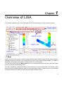

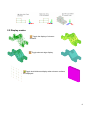
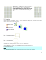
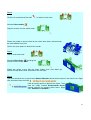

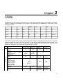
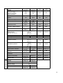


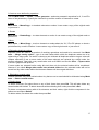
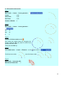
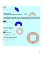
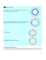
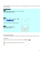
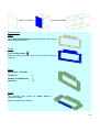
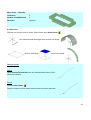
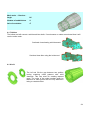
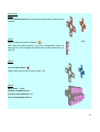
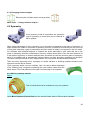
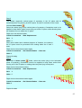
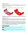
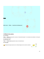
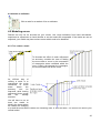
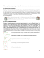
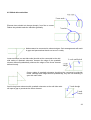
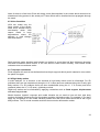
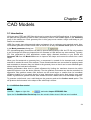
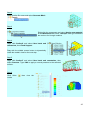
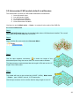
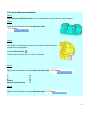
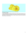


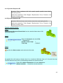
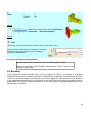
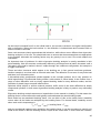


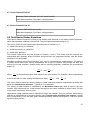
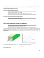


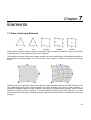
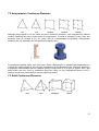
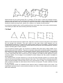
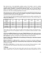
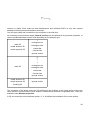

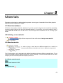
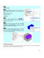

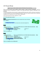

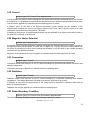
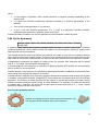

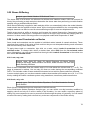
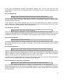
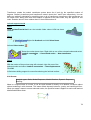
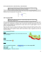
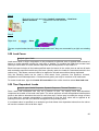
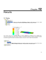
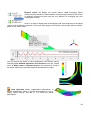
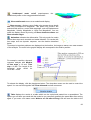

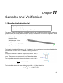
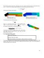
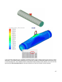
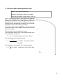
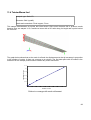

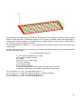
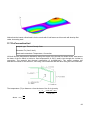
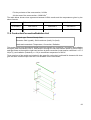

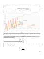
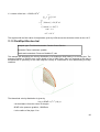
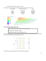
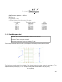
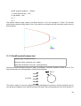
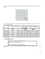
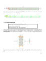
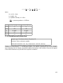
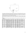
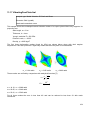

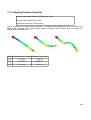
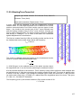
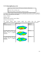
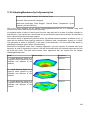
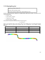

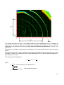
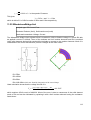
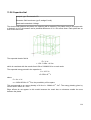
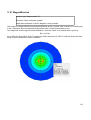

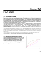
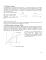


![[U7.05.21] Procédure IMPR_RESU (FORMAT `MED`)](http://vs1.manualzilla.com/store/data/006356529_1-18c585072845d4f1f91a14edb496c057-150x150.png)
![[U3.14.09] Modélisation 3D_ABSO](http://vs1.manualzilla.com/store/data/006354556_1-90d294b391fedb0a3a4ef0c43d87b2dc-150x150.png)
![[U3.14.01] Modélisations 3D et 3D_SI mécaniques](http://vs1.manualzilla.com/store/data/006353306_1-ee66ca199d5dc34d37fc69c57c8e21ef-150x150.png)