Download TSP 5.1 Reference Manual

TSP 5.1
Reference Manual
Bronwyn H. Hall
and
Clint Cummins
 TSP International 2009
Copyright  2009 by TSP International
Second printing, 2013. First edition (Version 4.0) published 1980.
TSP is a software product of TSP International. The information in this
document is subject to change without notice. TSP International assumes no
responsibility for any errors that may appear in this document or in TSP. The
software described in this document is protected by copyright. Copying of
software for the use of anyone other than the original purchaser is a violation
of federal law. Time Series Processor and TSP are trademarks of TSP
International.
ALL RIGHTS RESERVED
Table of Contents
Table Of Contents
1. Introduction____________________________________________ 1
Welcome to the TSP 5.1 Help System _________________________ 1
Introduction to TSP ________________________________________ 2
Examples of TSP Programs _________________________________ 3
Composing Names in TSP __________________________________ 4
Composing Numbers in TSP _________________________________ 5
Composing Text Strings in TSP ______________________________ 6
Composing TSP Commands _________________________________ 7
Composing Algebraic Expressions in TSP ______________________ 8
TSP Functions ___________________________________________ 10
Character Set for TSP _____________________________________ 11
Missing Values in TSP Procedures ___________________________ 13
LOGIN.TSP file __________________________________________ 14
2. Command summary ____________________________________ 15
Display Commands _______________________________________
Options Commands _______________________________________
Moving Data to/from Files Commands ________________________
Data Transformations Commands____________________________
Matrix Operations Commands _______________________________
Linear Estimation and Data Analysis Commands ________________
Nonlinear Estimation and Formula Manipulation Commands _______
QDV (Qualitative Dependent Variable) Commands ______________
Hypothesis Testing Commands______________________________
Forecasting and Model Simulation Commands __________________
Time Series Identification and Estimation Commands ____________
Control Flow Commands ___________________________________
Interactive Editing Commands and/or Data Commands ___________
Obsolete Commands ______________________________________
Cross-Reference Pointers __________________________________
15
16
17
18
19
20
21
22
23
24
25
26
27
28
29
3. Commands ___________________________________________ 31
ACTFIT ________________________________________________
ADD (interactive) _________________________________________
ANALYZ ________________________________________________
AR1 ___________________________________________________
31
33
35
41
i
Table of Contents
ARCH __________________________________________________ 49
ASMBUG _______________________________________________ 54
BJEST _________________________________________________ 55
BJFRCST_______________________________________________ 63
BJIDENT _______________________________________________ 68
CAPITL ________________________________________________ 72
CDF ___________________________________________________ 74
CLEAR (interactive) _______________________________________ 81
CLOSE_________________________________________________ 82
COINT _________________________________________________ 84
COLLECT (Interactive) ____________________________________ 95
COMPRESS ____________________________________________ 97
CONST ________________________________________________ 98
CONVERT ______________________________________________ 99
COPY_________________________________________________ 102
CORR/COVA ___________________________________________ 103
DATE _________________________________________________ 104
DBCOMP (Databank) ____________________________________ 105
DBCOPY (Databank) _____________________________________ 106
DBDEL (Databank) ______________________________________ 107
DBLIST (Databank) ______________________________________ 108
DBPRINT (Databank) ____________________________________ 109
DEBUG _______________________________________________ 110
DELETE _______________________________________________ 111
DELETE (Interactive) _____________________________________ 112
DIFFER _______________________________________________ 113
DIR (Interactive) ________________________________________ 116
DIVIND ________________________________________________ 117
DO ___________________________________________________ 120
DOC __________________________________________________ 122
DOT __________________________________________________ 123
DROP (Interactive) ______________________________________ 126
DUMMY _______________________________________________ 128
EDIT (Interactive) _______________________________________ 130
ELSE _________________________________________________ 133
END __________________________________________________ 134
ENDDO _______________________________________________ 135
ENDDOT ______________________________________________ 136
ENDPROC _____________________________________________ 137
ii
Table of Contents
ENTER (Interactive) _____________________________________
EQSUB _______________________________________________
EXEC (Interactive) _______________________________________
EXIT (Interactive) ________________________________________
FETCH ________________________________________________
FIML __________________________________________________
FIND (Interactive) _______________________________________
FORCST ______________________________________________
FORM ________________________________________________
FORMAT ______________________________________________
FREQ _________________________________________________
FRML _________________________________________________
GENR ________________________________________________
GMM _________________________________________________
GOTO ________________________________________________
GRAPH _______________________________________________
GRAPH (graphics version) ________________________________
HELP _________________________________________________
HIST __________________________________________________
HIST (graphics version) ___________________________________
IDENT ________________________________________________
IF ____________________________________________________
IN (Databank) __________________________________________
INPUT ________________________________________________
INST __________________________________________________
INTERVAL _____________________________________________
KALMAN ______________________________________________
KEEP (Databank) _______________________________________
KERNEL ______________________________________________
LAD __________________________________________________
LENGTH ______________________________________________
LIML __________________________________________________
LIST __________________________________________________
LMS __________________________________________________
LOAD _________________________________________________
LOCAL ________________________________________________
LOGIT ________________________________________________
LP ___________________________________________________
LSQ __________________________________________________
138
139
142
143
144
145
151
152
156
161
164
166
168
171
176
177
178
182
184
186
189
191
192
193
195
201
205
211
213
215
221
222
228
232
236
237
238
250
247
iii
Table of Contents
MATRIX _______________________________________________
MFORM _______________________________________________
ML ___________________________________________________
MMAKE _______________________________________________
MODEL _______________________________________________
MSD __________________________________________________
NAME ________________________________________________
NEGBIN _______________________________________________
Nonlinear Options _______________________________________
NOPLOT ______________________________________________
NOPRINT ______________________________________________
NOREPL ______________________________________________
NORMAL ______________________________________________
NOSUPRES____________________________________________
OLSQ _________________________________________________
OPTIONS______________________________________________
ORDPROB_____________________________________________
ORTHON ______________________________________________
OUT (Databank) ________________________________________
OUTPUT (Interactive) ____________________________________
PAGE _________________________________________________
PANEL ________________________________________________
PARAM _______________________________________________
PDL __________________________________________________
PLOT _________________________________________________
PLOT (graphics version) __________________________________
PLOTS ________________________________________________
POISSON _____________________________________________
PRIN _________________________________________________
PRINT ________________________________________________
PROBIT _______________________________________________
PROC ________________________________________________
QUIT (Interactive) _______________________________________
RANDOM ______________________________________________
READ _________________________________________________
RECOVER (Interactive) ___________________________________
REGOPT ______________________________________________
RENAME ______________________________________________
REPL _________________________________________________
iv
256
259
264
270
273
275
278
279
283
291
292
293
294
295
296
303
307
311
312
313
315
316
326
328
331
334
337
340
344
347
348
354
356
357
365
376
377
390
391
Table of Contents
RESTORE _____________________________________________
RETRY (Interactive) _____________________________________
REVIEW (Interactive) ____________________________________
SAMA _________________________________________________
SAMPSEL _____________________________________________
SAVE (Interactive) _______________________________________
SELECT _______________________________________________
SET __________________________________________________
SHOW ________________________________________________
SIML _________________________________________________
SMPL _________________________________________________
SMPLIF _______________________________________________
SOLVE ________________________________________________
SORT _________________________________________________
STOP _________________________________________________
STORE _______________________________________________
SUPRES ______________________________________________
SUR __________________________________________________
SYMTAB ______________________________________________
SYSTEM ______________________________________________
TERMINAL (Interactive) __________________________________
THEN _________________________________________________
3SLS _________________________________________________
TITLE _________________________________________________
TOBIT ________________________________________________
TREND _______________________________________________
TSTATS _______________________________________________
UNIT _________________________________________________
UNMAKE ______________________________________________
UPDATE (Interactive) ____________________________________
USER (Mainframe) ______________________________________
VAR __________________________________________________
WRITE ________________________________________________
YLDFAC_______________________________________________
392
393
394
395
397
401
402
403
405
407
412
414
416
421
423
424
425
426
428
430
431
432
433
436
437
441
443
444
445
447
448
449
454
458
4. Index _______________________________________________ 461
v
Introduction
Introduction
Welcome to the TSP 5.1 Help System
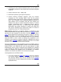
The TSP Help system contains the complete reference manual for TSP,
providing a description of every command and command option, organized
alphabetically by command. It is not intended as an introduction to the
program, nor as a tutorial for the inexperienced TSP user. To learn how to
use the program, you should obtain a copy of the TSP 5.1 User’s Guide
(available at http://www.tspintl.com/support/tsp/ug_online.htm) The User's
Guide contains more discussion and examples of how to combine TSP
statements and construct TSP programs.
The Help system can be useful in the following ways:

To read a basic introduction of what TSP and why it is useful, see
Introduction to TSP

To find out which command to use, see the functional index
Commands by Function.

You know which command or procedure you want to use, but are
unsure of the options available. You can look up the details of the
command in the Index (click on the Help Topics button above and
then click the Index tab) and check the Options.

To learn more about the methods used in any particular procedure.,
see the details in References under the command.

To see how to use a command, look at the Examples.

To check which results are stored after a procedure and how they
are named, consult the Output section of the command entry.

Basics gives complete definitions of TSP syntax, the interpretation of
special characters, and the mathematical and statistical functions
available.

If you want to find out something related to the use of TSP through
the Looking Glass, look it up in the TSP through the Looking Glass
section.

Examples of TSP Programs describes where to find sample TSP
programs.

You may also want to look at the TSP read me.
1
Introduction
Introduction to TSP
TSP provides regression, forecasting, and other econometric tools on
mainframe and personal computers. Areas where TSP can be useful
include:
Applied econometrics, including teaching
Macro-economic research and forecasting
Econometric analysis of cross section and panel data
Sales forecasting
Financial analysis
Cost analysis and forecasting
TSP is installed on thousands of computers worldwide. Although TSP was
developed by economists (starting with Version 1 in 1967) and most of its
uses are in economics, there is nothing in its design that limits its usefulness
to economic time series. Any statistical or econometric application involving
data sets of up to about 20,000 (or even more) observations is suitable for
TSP. For more information, prices, ordering, and upgrades, see our website,
http://www.tspintl.com.
2
Introduction
Examples of TSP Programs
TSP is a powerful program because it is not limited to its preprogrammed
commands. To help you develop your own specialized procedures we have
compiled some examples of TSP programs. The example programs can be
found in the
.......Program Files\TSP 5.1\examples
directory (the exact path may vary depending on where you installed TSP). If
you did a custom install of TSP, you may not have installed the examples. In
order to get the examples, you will have to reinstall TSP and do either a
"Typical" install or a "Custom" with the Examples option check-marked.
The TSP examples are further subdivided into five categories;
Miscellaneous, ML PROC, Panel Data, Qualitative Dependent Variables and
Time Series. Each of these categories has their own directory in the
Examples directory. For a description of each examples, look at the file
examples.txt in the Examples directory.
Updated examples may be found on the TSP International website at:
http://www.tspintl.com/examples
3
Introduction
Composing Names in TSP
Every name must begin with a letter, _ # % or @ (exceptions: 2SLS and
3SLS commands).
Subsequent characters in a name may be letters, _ # % @, or digits.
# or % may not be used in names that appear in MATRIX commands.
The maximum number of characters permitted in a name is 64 (in versions
prior to TSP 4.4 it was 8).
4
Introduction
Composing Numbers in TSP
Every number must begin with a ., +, -, or a digit.
No spaces may appear within a number.
One decimal point may appear.
One E or D may appear followed immediately by a one or two digit number
with or without a sign. This is interpreted as a power of 10 to multiply the first
number.
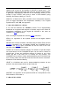
Example: 1E2 = 100.
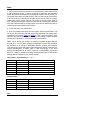
With free-format LOAD or READ commands, a . is interpreted as a missing
value, and a repeat count with a * may be specified.
The largest value of a series (in absolute value) that may be stored in TSP is
1.E-37, unless OPTIONS DOUBLE ; is used. Values larger than this are set
to missing. Scalars and matrices are always stored in double precision.
Examples:
3*0 is treated as 0 0 0
53 . 100 is treated as 53, missing, 100
5
Introduction
Composing Text Strings in TSP
A text string must be enclosed by matching pair of quotes (" or ').
Quotes are allowed in a string when they are of a different type from the
enclosing quotes, i.e. "Can't" or '"sometimes"' (interpreted as Can’t and
“sometimes”).
6
Introduction
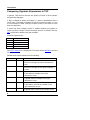
Composing TSP Commands

Every statement begins with a command name.
Exceptions:
X=Y;
X(I)=Y(I);
100 <statement>;
? implicit GENR
? implicit SET
? statement label for GOTO

The command name may be abbreviated, as long as it is uniquely
identified.

Many statements can have options specified in parentheses after
the command name. Option names may be abbreviated, like
command names. There are three kinds of options:
1. Boolean options, either on or off. On is specified by the
name of the option, as in PRINT, and off is specified by the
option name with NO in front of it, as in NOPRINT.
2. Options of the form option name = option value. The value
may be the name of a variable, a numerical value, or just a
keyword, depending on the context.
3. Options which give lists of variables, and are of the form
option name = (list of variables). Note that the parentheses
are required, unless the list contains only one name, or the
list is a listname.

A few commands can be followed by an algebraic formula: GENR,
SET, SMPLIF, SELECT, FRML, IDENT, IF, GOTO.

Most commands are followed by one or more series names,
separated by commas or spaces. These series names may include
lags. An implicit list (such as X1-X5) can be used directly in a
statement without making an intermediate listname. See the LIST
command for a complete description of implicit list syntax.

The end of a statement is marked by a semicolon (;) or dollar sign
($).
7
Introduction
Composing Algebraic Expressions in TSP
In general, TSP rules for formulas are similar to Fortran or other scientific
programming languages.
A lag is indicated by putting an integer or a name in parentheses after a
series name. The integer is negative for lags and positive for leads. A + sign
is not necessary for leads. If the lag or lead is a name, it must have no more
than four characters.
A series may have a single numeric or variable subscript (or lag/lead). A
matrix may have a single or double subscript (numeric or variable). See the
SET command for detailed rules and examples.
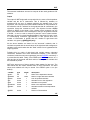
Arithmetic operators are:
+
*
/
** or ^
add
subtract
multiply
divide
raise to the power
See TSP Functions for a detailed list of functions and the MATRIX command
for matrix functions.
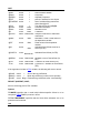
Relational and logical operators are the following:
Operator
=
.OP.
.EQ.
~= or ^=
.NE.
<
.LT.
>
.GT.
<=
.LE.
>=
.GE.
8
Description
gives the value 1 when the variables on the
left and on the right are equal; otherwise it is
zero
gives the value 1 when the variables on the
left and on the right are not equal; otherwise it
is zero
gives the value 1 when the variable on the left
is less than the variable on the right;
otherwise it is zero
gives the value 1 when the variable on the left
is greater than the variable on the right;
otherwise it is zero
gives the value 1 when the variable on the left
is less than or equal to the variable on the
right; otherwise it is zero
gives the value 1 when the variable on the left
is greater than or equal to the variable on the
Introduction
&
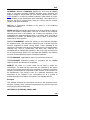
.AND.
|
.OR.
~ or ^
.NOT.
right; otherwise it is zero
gives the value 1 when both the variable on
the left and on the right are positive
gives the value 1 when both the variable on
the left and on the right are positive
gives the value 1 when the variable on the
right is negative or zero
Note: the .OP. form of the relational and logical operators is the alternative
to the symbolic notation (but it cannot be used in nested DOT loops).
As many parentheses as necessary may be used to indicate the order of
evaluation of a formula. The special parentheses [] and {} are treated as ().
In the absence of parentheses, evaluation proceeds from left to right in the
following order:
1
2
3
4
5
6
7
Functions
Exponentiation (**)
Multiplication and division
Addition, subtraction, and negation (unary -)
Relational operators
.NOT. (~)
.AND. (&) and .OR. (|)
9
Introduction
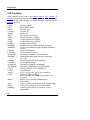
TSP Functions
These functions can be used in any GENR, FRML, IF, SET, SELECT, or
MATRIX command. Include the argument (value, series name, or algebraic
expression) in the parentheses(). For additional matrix functions, see the
MATRIX command.
LOG()
EXP()
ABS()
LOG10()
SQRT()
SIN()
COS()
TAN()
ATAN()
NORM()
CNORM()
CNORMI()
LNORM()
LCNORM()
DLCNORM()
CNORM2(.,.,.)
GAMFN()
LGAMFN ()
DLGAMFN()
TRIGAMMA()
FACT()
LFACT()
SIGN()
POS()
MISS()
INT()
CEIL()
ROUND()
10
Natural logarithm
Exponential function
Absolute value
Log base 10
Square root
Sine (argument in radians)
Cosine (argument in radians)
Tangent (argument in radians)
Arctangent (answer in radians)
Standard normal density
Standard normal cumulative distribution function
Inverse of the standard normal cumulative distribution
function
Log of normal density
Log of cumulative normal
Derivative of LCNORM = inverse Mills ratio
Standard bivariate normal cumulative distribution
(x1,x2,rho)
Gamma function (not Gamma density)
Log of Gamma function
Derivative of LGAMFN = DIGAMMA()
Derivative of DIGAMMA() [non-differentiable]
Factorial: FACT(X) = X! = GAMFN(X+1)
Log of factorial
Sign: -1 for X<0, 0 for X=0, 1 for X>0 [deriv=0]
Positive: POS(X) = max(0,X)
Note: "min(A,B)" = B - POS(B-A), "max(A,B)" = A +
POS(B-A)
Missing: 1 for X missing, 0 otherwise [nondifferentiable]
Integer: truncate (round towards 0) [non-differentiable]
Ceiling: round away from 0 [non-differentiable]
Round to nearest integer (.5 rounds to 1) [nondifferentiable]
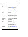
Introduction
Character Set for TSP
Character
Symbol
letter
A to
Z,_#%@
digit
0 to 9
decimal point
.
comma
,
colon
semicolon
dollar sign
quotation
mark
:
;
$
apostrophe
’
parentheses
() [] {}
"
question mark ?
plus sign
minus sign
star
slash
+
*
/
pound sign
#
percent
%
equal sign
=
ampersand
&
vertical bar
|
caret or hat
^
Use
Parts of names. Lowercase letters are allowed
on most computers; they are treated like
uppercase letters. # % cannot be used as part
of a name in the MATRIX command.
Parts of numbers or names
Marks the decimal point in numbers; sets off
logical operators; specifies string substitution
in the DOT procedure
Separates the words in a list and arguments in
multivariate functions like CNORM2; spaces
may be used, but commas are often preferred
for clarity
Part of date
Marks the end of a statement
Equivalent to ; . Semicolon is preferred.
Marks the beginning and end of a text string
(title or filename); specifies matrix inversion
Marks the beginning and end of a text string;
specifies matrix transposition
Encloses a list of options or expressions/lags
in algebraic formulas
Delimits the beginning of comments.
(Comments are terminated by the end of the
input line or logical record.)
Specifies addition
Specifies subtraction, a lag, or a list
Specifies multiplication or is part of power (**)
Specifies division
Matrix Kronecker product
Matrix Hadamard product (element by
element)
Specifies equality or definition of data;
relational operator (.EQ., .NE., .LE.,.GE.).
Logical operator (.AND.)
Logical operator (.OR.); Also used to separate
lists of variables in INST, KALMAN, LOGIT,
SAMPSEL, and VAR
Logical operator (.NOT., .NE.) or power (**),
11
Introduction
tilde
less than
greater than
continuation
miscellaneous
12
~
<
>
\
!`
depending on context
Logical operator (.NOT., .NE.)
Relational operator (.LT., .LE.)
Relational operator (.GT., .GE.)
Continuation of a line (interactive)
Reserved for future use
Introduction
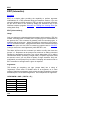
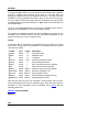
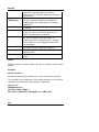
Missing Values in TSP Procedures
Procedures that drop
observations containing
missing values
AR1, OLSQ, INST, 2SLS, LIML,
LAD
LSQ, FIML, GMM, ML, SUR, 3SLS
PROBIT, TOBIT, SAMPSEL,
LOGIT
CONVERT, FORCST, GENR
MSD, CORR, COVA, MOM
GRAPH, PLOT, HIST
PANEL, VAR
Procedures that cannot execute if
the sample contains missing
values
ACTFIT
BJEST, BJIDENT, BJFRCST
COINT, UNIT
ARCH, KALMAN
DIVIND, SAMA
SOLVE, SIML
PRIN
13
Introduction
LOGIN.TSP file
login.tsp is a special INPUT file; it is read automatically at the start of
interactive sessions and batch jobs. This is useful for setting default options
for a run.
If you use the same options repeatedly, you may want to place them in a
login.tsp file. Every time TSP starts, it checks for a login.tsp file, and
executes it first. Normally, TSP looks for login.tsp in your working
directory. If it does not find one, it looks in the directory in which you
installed TSP for DOS and Windows, in the folder in which you installed TSP
for Macs, and in the home directory on Unix.
Commands which can be usefully issued in a login.tsp file are the following
OPTIONS MEMORY= approximate memory to be used by TSP (in
Megabytes). This option only works if OPTIONS is the first command in the
run, or the first command in the login.tsp file.
INPUT some file that transforms the data or selects the data you are using
for a number of TSP programs.
14
Command summary
Command summary
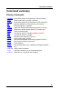
Display Commands
ASMBUG
DATE
DEBUG
DIR
DOC
GRAPH
GRAPH
HELP
HIST
HIST
NAME
PAGE
PLOT
PLOT
PRINT
SHOW
SYMTAB
TITLE
TSTATS
prints debug output during parsing of TSP commands
prints current date on screen or printout
prints debug output during execution of TSP commands
lists files available in current directory (interactive)
adds descriptions to variables
graph one variable against another (graphics version)
graphs one variable against another in a scatter plot
prints command syntax
one-way bar chart for variable (graphics version)
one-way bar chart for variable
specifies name and title for TSP run
starts a new page in printout
plots several variables versus time (graphics version)
plots several variables versus time
prints variables
lists currently defined TSP variables by category (SERIES,
etc.)
debug version of SHOW
specifies new title for run or immediate printing
prints table of coefficients and t-statistics
15
Command summary
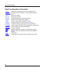
Options Commands
FREQ
NOPLOT
NOREPL
OPTIONS
PLOTS
REPL
SELECT
SMPL
SMPLIF
16
set the data frequency (None, Annual, Quarterly, Monthly)
turns residual plots off (OLSQ, INST, AR1, LSQ)
prevents splicing of series, generates missing values instead
general option setting -- CRT, HARDCOPY, LIMPRN, etc.
turns residual plots off (OLSQ, INST, AR1, LSQ)
allows updating of series during GENR (the default)
restricts the set of observations to those meeting a condition
set the sample of observations to be processed
same as SELECT, but restricts starting from current sample
Command summary
Moving Data to/from Files Commands
CLOSE
DBCOMP
DBCOPY
DBDEL
DBLIST
DBPRINT
FETCH
FORMAT
IN
KEEP
LOAD
NOPRINT
OUT
PRINT
READ
RECOVER
RESTORE
SAVE
STORE
WRITE
closes an external input or output file
compresses a databank (Databank)
copies databank for moving to another computer
(Databank)
deletes variables from a databank (Databank)
lists all variable names in a databank (Databank)
prints all series in a databank (Databank)
reads a microTSP-format databank
(option) -- used in READ and WRITE with numbers
causes automatic searching of databanks listed
(Databank)
stores TSP variables on specified OUT files
(Databank)
reads variables from a file (or from program) - same
as READ
suppresses echoing of commands in a LOAD
section
causes automatic databank storage in files listed
(Databank)
same as WRITE
reads variables from a file (or from program)
recovers lost program from INDX.TMP file
(Interactive)
reads variables from a SAVE file into the program
(Interactive)
saves all current variables on disk (Interactive)
writes a microTSP-format databank
writes variables to a file (or to printout)
17
Command summary
Data Transformations Commands
CAPITL
accumulates a capital stock from an investment series
CONVERT changes a series from higher to lower frequency (stock or
flow)
COPY
copies any variable
DELETE
deletes any variables
DIVIND
computes Divisia price and quantity indices
DUMMY
makes dummy variables from a series
GENR
creates a series using an algebraic formula
LENGTH
computes length of a TSP list (useful in PROCs)
NORMAL normalizes a series (usually a price index, via division)
RANDOM random number generator: normal (univariate or multivariate),
uniform, Poisson, or empirical (bootstrap)
RENAME renames a variable
SAMA
Seasonal adjustment using the moving average method
SET
modify a scalar or series/matrix element with an algebraic
formula
SORT
sorting data
TREND
create linear trend variable (can be repeating like months)
18
Command summary
Matrix Operations Commands
MATRIX
MFORM
MMAKE
ORTHON
UNMAKE
YLDFAC
matrix algebra and transformations
change dimensions or type of matrix
create a matrix from several series or a vector from
scalars
orthonormalization
create several series from a matrix or scalars from a
vector
LDL' decomposition (symmetric indefinite matrix)
19
Command summary
Linear Estimation and Data Analysis Commands
CORR
COVA
INST
KERNEL
LAD
LIML
LMS
LP
MSD
OLSQ
PANEL
PDL
PRIN
20
correlation matrix of several series
covariance matrix of several series
instrumental variables and two stage least squares regression
computes a Kernel density estimation or regression
Least Absolute Deviations estimation (median regression)
Limited Information Maximum Likelihood
Least Median Squares estimation
Linear programming (with constraints)
mean, standard deviation, minimum, maximum, sum, variance,
skewness, kurtosis for a list of series
Ordinary Least Squares (linear regression), can use weights
panel data estimation (total, within, between, variance
components)
describes specification of Polynomial Distributed Lag variables
(Almon lags), and Shiller Lags; used in OLSQ, INST, AR1,
PROBIT, TOBIT
Principal Components (simple factor analysis)
Command summary
Nonlinear Estimation and Formula Manipulation
Commands
CONST
DIFFER
EQSUB
FIML
FRML
GMM
IDENT
LSQ
ML
MLPROC
NONLINEAR
options
PARAM
SUR
3SLS
defines scalars as fixed (non-estimable) constants
create equations with analytic derivatives of formulas
(FRMLs)
equation substitution, one formula into another
Full Information Maximum Likelihood estimation (system
of linear or nonlinear equations, identities, implicit
equations, general cross-equation restrictions,
Multivariate Normal errors)
define a linear or nonlinear equation for estimation
Generalized Method of Moments estimation, nonlinear,
with heteroskedasticity- and autocorrelation-robust
standard errors
same as FRML but for an identity -- no implied
disturbance (for FIML)
minimum distance estimation of single or multiple
equation linear or nonlinear equations, general crossequation restrictions, additive error terms (see SUR,
3SLS also)
Maximum Likelihood estimation, log likelihood specified
in FRML
Maximum Likelihood estimation, log likelihood specified
in a PROC
describes iteration methods and options used by ARCH,
BJEST, LSQ, FIML, LOGIT, ML, MLPROC, PROBIT,
TOBIT, SIML, SOLVE
defines scalars as estimable parameters, can supply
starting values
Seeming Unrelated Regressions -- LSQ without
instruments
Three Stage Least Squares -- LSQ with instruments
21
Command summary
QDV (Qualitative Dependent Variable) Commands
INTERVAL
LOGIT
NEGBIN
NONLINEAR
options
ORDPROB
POISSON
PROBIT
SAMPSEL
TOBIT
22
estimates the Interval model (ordered Probit with
known limits)
estimates binary, multinomial, conditional, and mixed
Logit models
estimates the Negative Binomial regression model for
count data
describes iteration methods used by ARCH, BJEST,
LSQ, FIML, LOGIT, PROBIT, TOBIT, and ML
estimates the Ordered Probit model
estimates the Poisson model for count data
estimates the Probit model (0/1 with normal error term)
estimates a two-equation Sample Selection model
estimates the Tobit model (0/positive with normal error
term)
Command summary
Hypothesis Testing Commands
ANALYZ
CDF
COINT
REGOPT
computes standard errors for functions of parameters
from a previous estimation
distribution functions and P-values
unit root and cointegration tests
controls printing and storage of regression diagnostics
23
Command summary
Forecasting and Model Simulation Commands
ACTFIT
BJFRCS
T
FORCST
FORM
MODEL
SIML
SOLVE
24
compares actual and forecasted series
forecasts Box-Jenkins ARIMA models
computes forecasts for estimated linear models (OLSQ, INST,
AR1)
constructs an equation (FRML) from an estimated linear model
orders large simultaneous equation systems for use by
SOLVE
simulation of general nonlinear systems of equations
simulation of large (usually sparse) systems of equations
Command summary
Time Series
Commands
AR1
ARCH
BJEST
BJFRCST
BJIDENT
COINT
KALMAN
UNIT
VAR
Identification
and
Estimation
regression with correction for AR(1) (autocorrelated) error
estimates GARCH-M models
estimates Box-Jenkins ARIMA models
forecasts Box-Jenkins ARIMA models
identifies the order of Box-Jenkins ARIMA models
unit root and cointegration tests
Kalman filter estimation
synonym for COINT
Vector autoregressions
25
Command summary
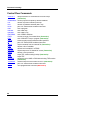
Control Flow Commands
COLLECT
delays execution of commands such as DO loops
(Interactive)
COMPRESS clears up space occupied by deleted variables
DO
defines a (numeric-indexed) DO loop
DOT
defines a (character-indexed) DOT loop
ELSE
part of IF-THEN-ELSE conditional structure
END
end of program
ENDDO
end of DO loop
ENDDOT
end of DOT loop
ENDPROC
end of PROC definition
EXEC
execute a range of command lines (Interactive)
EXIT
end of COLLECT loop or program (Interactive)
GOTO
starts execution at the statement label specified
IF
part of IF-THEN-ELSE conditional structure
INPUT
read commands from an external file (Interactive)
LIST
defines a list of variables
LOCAL
defines local variables in a PROC
OUTPUT
directs output to a file instead of screen (Interactive)
PROC
defines a user procedure
QUIT
stops TSP, without saving backup (Interactive)
STOP
stops TSP
SYSTEM
temporary exit to VMS or DOS without losing TSP session
(Interactive)
TERMINAL
restores output to screen after OUTPUT (Interactive)
THEN
part of IF-THEN-ELSE conditional structure
USER
user-programmable command (Mainframe)
26
Command summary
Interactive Editing
Commands
ADD
CLEAR
DELETE
DROP
EDIT
ENTER
FIND
RETRY
REVIEW
UPDATE
Commands
and/or
Data
adds arguments to previous command (Interactive)
clears TSP's memory (data storage) (Interactive)
deletes lines during execution (Interactive)
deletes arguments from previous command (Interactive)
edits a command (Interactive)
enter data for a series (Interactive)
lists lines containing a specific TSP command
(Interactive)
edits previous command and re-executes it (Interactive)
lists range of TSP command lines (Interactive)
replaces observations in a series (Interactive)
27
Command summary
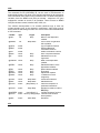
Obsolete Commands
Old command
Replacement command
INPROD x y z;
INV a ai deta;
MADD x y z;
MAT z = x'y
MAT ai = a"; MAT deta =
DET(a)
MAT z = x+y;
MATRAN x xt
MAT xt = x';
MDIV x y z;
MAT z = x/y;
MEDIV x y z;
MAT z = x/y;
MEMULT x y z;
MAT z = x%y;
MMULT x y z;
MAT z = x*z;
MSQUARE x y;
MAT y = x'x;
MSUB x y z;
MAT z = x-y;
NOSUPRES x;
REGOPT x;
SUPRES x;
REGOPT (NOPRINT) X;
VGVMLT x y z;
MAT = z*y ;
YFACT x y;
MAT y = CHOL(x)
YINV a ai;
MAT ai = YINV(a)
YQUAD x y z;
MAT z = x*y*x';
28
Command summary
Cross-Reference Pointers
Command synonyms
For
LOAD
COVA
CORR
NOSUPRES
PRINT
SUPRES
See
READ
MSD
MSD
REGOPT (PRINT)
WRITE
REGOPT
(NOPRINT)
INST
COINT
2SLS
UNIT
Non-command entries
For
Functions
FORMAT
NONLINEAR
PDL
See
BASIC RULES
READ and WRITE
convergence options used in: LSQ, ML, FIML,
BJEST, etc.
Polynomial Distributed Lags used in: OLSQ, AR1,
etc.
Examples
For examples of
AR1
CDF
DOT
ELSE
EQSUB
FRML
GENR
IF
INST
LIST
LOGIT
LSQ
MAT
OLSQ
See
FORM, PDL
RANDOM
ELSE, LIST,SORT
GOTO
ANALYZ, ML
FORM, LIST
DIFFER
GOTO
PDL
DUMMY, LENGTH
MMAKE
ANALYZ, EQSUB
MMAKE, ORTHON
PDL
29
Command summary
PROC
RETRY
SET
THEN
30
LOCAL
ADD, DROP, EDIT
DO
GOTO
ACTFIT
Commands
ACTFIT
Options
Example
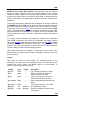
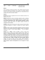
References
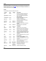
ACTFIT computes and prints a variety of goodness-of-fit statistics for the
actual and predicted values of a series. Theil (references below) suggests
using these statistics for evaluating an estimated time series equation or
forecast.
ACTFIT (SILENT,TERSE) <actual series name> <predicted series
name> ;
After ACTFIT, give the name of the actual data series followed by the name
of the fitted or predicted series.
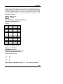
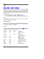
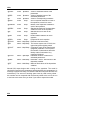
Output
ACTFIT prints a title, the names of the series being compared, the time
period (sample) over which they are compared, and then a variety of
computed statistics on the comparison. These include the correlation of the
two series, the mean square error, the mean absolute error, Theil's
inequality coefficient (U), changes and percent changes in U, and a
decomposition of the source of the discrepancies between the two series:
differences in the mean, or differences in the variance.
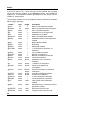
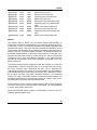
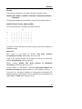
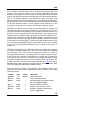
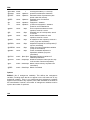
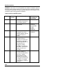
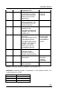
The following scalar results are stored by ACTFIT:
variable
@R
@R2
@RMSE
@MSE
@MAE
@ME
@RMSPE
@MSPE
@MAPE
@MPE
@BETA
@U66
length
1
1
1
1
1
1
1
1
1
1
1
1
@U66P
1
@FBIAS
1
description
Correlation coefficient
Correlation coefficient squared
Root mean square error
Mean squared error
Mean absolute error
Mean error
Root-Mean-Squared Percent Error
Mean-Squared Percent Error
Mean Absolute Percent Error
Mean Percent Error
Regression coef. of Actual on Predicted
Theil's U Inequality coef.
(Changes)
U66
Theil's U Ineq. coef. (Percent
changes) U66P
Fraction of MSE due to Bias
31
ACTFIT
@FDVAR
1
@FDCOV
1
@FDB1
1
@FRES
1
Fraction of MSE due to different
Variation
Fraction of MSE due to difference
Covariation
(Alt.Decomp.) Frac. due to Diff. of BETA
from 1
(Alt.Decomp.) Frac. due to Residual
variance
Note
U is defined differently in the 1961 and 1966 references. The 1966 definition
is used in TSP Versions 4.0 and 4.1; under this definition U can be greater
than one. In TSP Version 4.2 and above, both versions of U are printed. This
output is followed by a time series residual plot of the two series if the
PLOTS option is on (see the OPTIONS command). If the RESID option is
on, the residual series will be stored under the name @RES, whether or not
the PLOTS option is on.
Options
SILENT/NOSILENT suppresses all printed output.
TERSE/NOTERSE prints a reduced output.
Example
ACTFIT R RS ;
References
Theil, Henri, Economic Forecasts and Policy, North Holland Publishing
Company, 1961.
Theil, Henri, Applied Economic Forecasting, North Holland Publishing
Company, 1966.
32
ADD
ADD (interactive)
Examples
ADD adds a list of variables to the previous statement and re-executes it. It
is the opposite of DROP.
ADD <list of variables> ;
ADD offers a convenient means of adding variables to a regression and
performing a second estimation (without having to fully retype the
command). It is not, however, restricted to this usage, and may be used in
any circumstance where this type of command modification is needed.
The command
ADD var1 var2
and the sequence
RETRY
>> INSERT var1
>> INSERT var2
>> EXIT
are identical in function since both permanently modify the previous
command by inserting var1 and var2 at the end of the command. The
command is then automatically executed in both cases. The only potential
difference between these approaches (besides the amount of typing) is in
the definition of "previous". RETRY with no line number argument assumes
you want to modify the last line typed. ADD will not accept a line number
argument, and always modifies the last line that is not itself an ADD (or
DROP) command.
ADD and DROP allow you to execute a series of closely related regressions
by entering the first estimation command, followed by a series of ADD and
DROP commands. Since each ADD or DROP permanently alters the
command, each new modification must take all previous modifications into
account.
Notes
It is not possible to combine ADD and DROP into one step to perform a
replace function, or to make compound modifications to a command. In
these circumstances, RETRY must be used.
Examples
33
ADD
OLSQ (WEIGHT=POP) YOUNG,C,RSALE,URBAN,CATHOLIC
ADD MARRIED
will run two regressions, the second of which is:
OLSQ (WEIGHT=POP) YOUNG,C,RSALE,URBAN,CATHOLIC,MARRIED
This is also how the command will now look if you REVIEW it, since it has
been modified and replaced both in TSPs internal storage and in the backup
file.
Another use for ADD might be in producing plots. The following will produce
two plots with the same option settings, but two series are added to the
second plot.
PLOT (MIN=500,MAX=1500,LINES=(1000)) GNP G GNPS H
ADD CONS C CONSS D
34
ANALYZ
ANALYZ
Output
Options
Examples
References
ANALYZ computes the values and estimated covariance matrix for a set of
(nonlinear) functions of the parameters estimated by the most recent OLSQ,
LIML, LSQ, FIML, PROBIT, etc. procedure. It also computes the Wald test
for the hypothesis that the set of functions are jointly zero. If the functions
are linear, after an OLSQ command, the F test of the restrictions, and
implied restricted original coefficients will be printed. ANALYZ can also be
used to compute values and standard errors for function of parameters and
series; in this case the result will be two series, one containing the values
corresponding to each observation, and the other the standard errors.
The method used linearizes the nonlinear functions around the estimated
parameter values and then uses the standard formulas for the variance and
covariance of linear functions of random variables. See the references for
further discussion of this "delta method". TSP obtains analytic derivatives
internally for the nonlinear functions. ANALYZ can also be used to
select/reorder a subset of a VCOV matrix and COEF vector, for use in
making a Hausman specification test.
ANALYZ (COEF=<input parameter vector>, HALTON, NAMES=(<list of
names>), NDRAW=<number of draws>, PRINT, PRMEAN,
PRSERIES, SILENT, VCOV=<matrix name>) <list of equation
names> ;
Usage
ANALYZ is followed by a list of equation (FRML) names. After estimation
procedures with linear models (OLSQ, INST, LIML, PROBIT, ...), these
equations specify functions of the estimated coefficients which are to be
computed by referring to the coefficients by the names of the associated
variables. After estimation procedures with nonlinear models (LSQ and
FIML), the equations specify functions of the estimated parameters.
ANALYZ has no provision for combining the variances from more than one
estimation, because it cannot obtain the associated covariance of the
coefficient estimates. The equations must be previously defined by FRML
statements; if the FRML statements have variable names on the left hand
side, the computed value of each function will be stored under that variable
name.
35
ANALYZ
If series names (other than the names of right hand side variables from the
previous OLSQ, INST, LIML, or PROBIT estimation) are included in the
FRML(s), a series of values will result. One application for this kind of FRML
is an elasticity which depends on estimated parameters, and also on data
such as income. ANALYZ will compute the standard errors for such a FRML
using the covariance matrix of the estimated parameters, and treating the
data as fixed constants. See the example below of computing an elasticity
series.
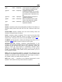
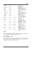
Output
If the PRINT option is on, ANALYZ prints a title, the names of the input
parameters, the equations in symbolic form, a table of the derived functions
and their standard errors, and the chi-squared value of a test that the
functions are jointly zero. This chi-squared has degrees of freedom equal to
the number of equations. The P-value (significance level) for the chi-squared
test is also printed. If the print option is off (the default), only the derived
functions and the chi-squared test are printed.
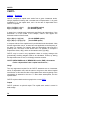
ANALYZ also stores the calculated parameters and their variances in data
storage as though they were estimation results, whether or not the PRINT
option is on. The results are stored under the following names.
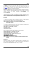
variable
@RNMSA
type
list
@WALD
@NCOEFA
scalar
scalar
@NCIDA
%WALD
scalar
scalar
@COEFA
vector
@SESA
vector
@TA
vector
%TA
vector
@MSD
matrix
@VCOVA
matrix
36
length
#eqs
description
Names of derived
parameters.
1
Value of Wald test.
1
Number of derived
parameters.
1
Degrees of freedom.
1
P-value (significance) of
Wald test.
#eqs
Values of derived
parameters.
#eqs
Standard errors of derived
parameter.
#eqs
T-statistics (asymptotically
normal).
#eqs
p-values corresponding to
@TA
#eqs*8
Matrix of simulation results
when NDRAW option is
used.
#eqs*#eqs Estimated variance
covariance of derived
ANALYZ
parameters.
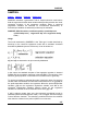
Method
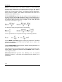
Assume that a previous estimation in TSP has stored a vector of K
parameter estimates b stored in @COEF and their variance covariance
matrix Var(b) stored in @VCOV. Values and standard errors for the M
functions f(b) are desired. To compute these, ANALYZ obtains the first
derivatives of f with respect to b analytically:
The functions f(b) and the matrix G are evaluated at the current values of b
and any constants or data values which may appear in f(b). The variancecovariance matrix for f(b) is then (asymptotically, or exactly if f(b) is linear in
b) defined as
This is known as the "delta method". For example, if M=1 and f(b) = f1 =
2*b1, then G=2 (with zeros elsewhere if K>1), and Var(f1) = 4*Var(b1) .
If the equations are linear, and an OLSQ command was used for estimation,
ANALYZ prints the F-statistic for the set of joint restrictions (@FST =
@WALD/@NCIDA). In addition, ANALYZ computes and prints the implied
restricted original coefficients and their standard errors. These are stored
under @COEFC, @VCOVC, etc.
Options
COEF= vector containing the values of the parameters in the equations to
be analyzed. This vector should correspond to the parameters listed in the
NAMES= option, and also to the supplied VCOV matrix. The default is
@COEF.
HALTON specifies that a (shuffled) Halton sequence is used for the random
draws when the NDRAW option is given. This provides more uniform
coverage of the range of values, so it may yield more accurate integration for
a given number of draws.
NAMES= specifies an optional list of parameter names which are the labels
for an associated covariance matrix supplied by the VCOV= option. The
default is @RNMS.
37
ANALYZ
NDRAW=n computes asymmetric confidence intervals for nonlinear
functions by drawing n simulated parameter vectors. These functions can
vary over time as well. This is an alternative to the default "delta method"
which uses derivatives and is exact for linear functions. The percentiles
2.5% and 97.5% are computed, to construct a two-tailed confidence interval
at the 95% significance level. A matrix named @MSD with columns
SE T LB2.5% UB97.5% MEAN MIN MAX NUM_GOOD is
stored. NUM_GOOD is the number of nonmissing results computed.
Numeric errors such as division by zero result in missing values. When
ANALYZ is used with series and NDRAW, the results are stored in series
whose names are the name of the parameter computed followed by _SE _T
_LB _UB _MEAN _MIN _MAX _NG. See the Examples for an illustration.
PRINT/NOPRINT tells whether or not the ANALYZ input is to be printed.
Under the default, NOPRINT, only the results are printed.
PRMEAN/NOPRMEAN tells whether summary statistics (mean, standard
deviation, minimum, maximum, and median) are to be computed for the
derived series when ANALYZ is used on equations containing series.
PRMEAN is true by default.
PRSERIES/NOPRSERIES tells whether the computed series are to be
printed when ANALYZ is used on equations containing series. The default
for PRSERIES is TRUE when the number of observations is less than or
equal to 100 and FALSE otherwise.
SILENT/NOSILENT specifies that no output is to be produced. The results
are stored under the names @RNMSA, @COEFA, etc. Note that
REGOPT(NOPRINT) COEF; is also needed, to suppress printing of the table
of coefficients.
VCOV= specifies the name of a variance-covariance matrix of the input
parameters (whose names are given by NAMES=). The use of these two
options enables one to do an ANALYZ on matrices other than the @VCOV
matrix from a standard estimation procedure. The default is @VCOV.
Examples
Obtain "long-run" coefficients for models with lagged dependent variables:
FRML LR1 ALPHALR = ALPHA/(1-LAMBDA) ;
FRML LR2 PHILR = PHI/(1-PSI) ;
ANALYZ LR1,LR2 ;
See the EQSUB command for an example of using ANALYZ (with EQSUB)
to evaluate and obtain standard errors for restricted parameters in a translog
system.
38
ANALYZ
The next example shows how to calculate an elasticity (and its standard
errors) when the elasticity changes over the sample.
FRML EQ1 LQ1 = A1 + B1*LP1 + B2*LP2 + B12*LP1*LP2 +
B13*LP1*LP3 + B23*LP2*LP3;
FRML EL1 ELD1 = B1 + B12*LP2 + B13*LP3; ? d(LQ1)/d(LP1)
SMPL 48,95;
LSQ EQ1;
? Obtain and plot elasticity for each year between 1948 and 1995:
SMPL 48,95;
ANALYZ (NOPRSER) EL1;
PLOT ELD1 ;
? Compute the average elasticity and its average s.e. - not needed in
v5.1 and later, as this is automatic.
MSD ELD1 ELD1_SE ;
Here is an example of using ANALYZ after OLSQ. It computes a chi-squared
test of the hypothesis that the sum of the two coefficients is zero (this test
statistic equals the standard F-statistic).
OLSQ Y C X1 X2 ;
FRML SUM X1+X2 ;
ANALYZ SUM ;
Suppose that we want to extract a few parameters and their associated
VCOV matrix from a system with a large number of parameters in arbitrary
order:
SUPRES COEF;
LSQ (SILENT) EQ1-EQ50; ? estimation with a large number of
equations
SUPRES;
DOT B1-B5;
FRML EQ. . = . ;
? construct FRML EQB1 B1 = B1; etc.
ENDDOT;
ANALYZ EQB1-EQB5;
? print results for 5 of the parameters only
RENAME @VCOVA VCVB1_5; ? for use later
RENAME @COEFA CB1_B5;
Here is an example using random draws to compute asymmetric confidence
intervals:
FRML EQ1 Y = A+B*X;
LSQ EQ1;
FRML EQS SUM = A+B;
FRML EQR RATIO = A/B;
ANALYZ(NDRAW=500) EQS EQR;
39
ANALYZ
In this example, the scalars SUM and RATIO will be stored, and eight
statistics on the 500 computations of the two functions will be printed and
stored in the 2 x 8 matrix @MSD.
An example of series output and random draws:
PROBIT D C X;
FRML EQP P = CNORM(A+B*X);
ANALYZ(NDRAW=200,NAMES=(A,B)) EQP;
In
this
example
the
series
P P_SE P_T P_LB P_UB P_MEAN P_MIN P_MAX P_NG will be stored
and printed.
References
Bishop, Y. M. M., S. E. Fienberg, and P. W. Holland, Discrete Multivariate
Analysis: Theory and Practice, MIT Press, Cambridge, MA, 1975, pp. 486502.
Gallant, A. Ronald, and Dale Jorgenson, "Statistical Inference for a System
of Simultaneous, Non-linear, Implicit Equations in the Context of
Instrumental Variable Estimation", Journal of Econometrics 11, 1979, pp.
275-302.
Gallant, A. Ronald, and Alberto Holly, "Statistical Inference in an Implicit,
Nonlinear, Simultaneous Equation Model in the Context of Maximum
Likelihood Estimation", Econometrica 48, 1980, pp. 697-720.
40
AR1
AR1
Output
Options
Examples
References
AR1 obtains estimates of a regression equation whose errors are serially
correlated. These estimates are efficient if the disturbances in the equation
follow an autoregressive process of order one. The estimates may be
obtained using one of two different objective functions: exact maximum
likelihood (which imposes stationarity by constraining the serial correlation
coefficient to be between -1 and 1 and keeps the first observation for
estimation), or by Generalized Least Squares (GLS), which drops the first
observation.
AR1 (FAIR, FEI. INST=(list of instrumental variables), METHOD=CORC
or HILU or ML or MLGRID, OBJFN= EXACTML or GLS, REI,
RMIN=<minimum rho value>, RMAX=<maximum rho value>,
RSTART=<start value for rho>, RSTEP=<step value for rho>,
TSCS, nonlinear options) <dependent variable name> <list of
independent variables> ;
To obtain estimates of a regression equation which are corrected for first
order serial correlation, use the AR1 command as you would an OLSQ
command. PDL (polynomial distributed lag) variables may be included in an
AR1 statement. See the PDL section for a further description of how to
specify these variables. TSP automatically deletes observations with missing
values for one or more variables before estimation.
When the SMPL frequency is type PANEL, AR1 can also obtain estimates
for a panel data model with fixed (FEI) or random (REI) effects. AR1
estimates can also handle plain time series which have irregular spacing
(gaps in the SMPL).
Output
The AR1 procedure produces output that is similar to OLSQ and LSQ
(including the iteration log). The equation title and the chosen objective
function (method of estimation) are printed first. If the PRINT option is on,
this is followed by the list of option values, the starting values for all the
coefficients, iteration output for all coefficients, and any grid values for rho
and the objective function.
41
AR1
The usual regression output follows, as described under the OLSQ
command. The regression statistics are computed from the fitted values and
residuals described below. If the objective function chosen was GLS, a
common factor test is included in the regression statistics. This test is a
likelihood ratio test of the restrictions implied by AR(1) compared to an
unconstrained OLS model that includes the lagged dependent as well as the
current and lagged right hand side variables. [The test is not well-defined
when the model is estimated by ML due to the special treatment of the first
observation].
As in OLSQ and INST, a table of coefficient estimates is printed. RHO is
always the last coefficient in the table; its inclusion guarantees that the
standard errors are always consistent, even if there are lagged dependent
variables on the right hand side. The fitted values (@FIT) and residuals
(@RES) are computed as follows:
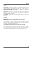
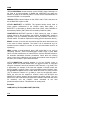
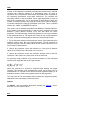
AR1 also stores this regression output in data storage for later use. The
table below lists the results available after an AR1 command. Note: the
number of coefficients (# vars) always includes RHO.
variable
@RNMS
@LHV
@RHO
type
list
list
scalar
length
#vars
1
1
@SSR
@S
@YMEAN
scalar
scalar
scalar
1
1
1
@SDEV
scalar
1
@NOB
@DW
@RSQ
@ARSQ
@IFCONV
scalar
scalar
scalar
scalar
scalar
1
1
1
1
1
@LOGL
@COMFAC
scalar
scalar
1
1
42
description
Names of right hand side variables
Name of the dependent variable
Serial correlation parameter at
convergence
Sum of squared residuals
Standard error of regression
Mean of the transformed dependent
variable
Standard deviation of the dependent
variable
Number of observations
Durbin-Watson statistic
R-squared
Adjusted R-squared
=1 if convergence achieved, =0
otherwise
Log of likelihood function.
Common factor test (if OBJFN=GLS)
AR1
@COEF
@SES
@T
%T
@COEFAI
@SESAI
vector
vector
vector
vector
vector
vector
@TAI
%TAI
@VCOV
vector
vector
matrix
@AI
series
@RES
@FIT
series
series
#vars
#vars
#vars
#vars
#vars
#vars
Coefficient estimates.
Standard Errors.
t-statistics.
p-values for t-statistics.
Fixed effect estimates (FEI)
Standard Errors on fixed effects
(FEI).
#vars
t-statistics on fixed effects (FEI).
#vars
p-values for t-statistics on FEs (FEI).
#vars*#vars Variance-covariance of estimated
coefficients.
#obs
Fixed effect for each obs, in series
form (FEI)
#obs
Fitted residuals from model.
#obs
Fitted values of dependent variable.
If the regression includes PDL variables, @SLAG, @MLAG, and @LAGF
will also be stored (see OLSQ for details).
Method
AR1 uses an initial grid search to local possible multiple local optima (when
OBJFN = GLS), and then iterates efficiently to a global optimum with second
derivatives. The likelihood function and treatment of the initial observation
are described completely in Davidson and MacKinnon (1993).
When OBJFN=EXACTML (the default), AR! simply maximizes the likelihood
function for disturbances that follow a stationary autoregressive process with
respect to the serial correlation rho and the coefficients of the independent
variables.
For panel data, AR1 with fixed (FEI) or random (REI) effects is similar to the
corresponding PANEL regressions, but with an added AR(1) component.
The random effects estimator follows Baltagi and Li (1991). It uses analytic
second derivatives to obtain quadratic convergence and accurate t-statistics
for all parameters (including RHO and RHO_I, the intraclass correlation
coefficient, which can be negative). After the fixed effects AR1 estimator, the
estimated fixed effects are stored in the matrix @COEFAI and in the series
@AI.
Options
43
AR1
FAIR/NOFAIR specifies whether the lagged dependent and independent
variables are to be added to the instrument list automatically when doing
instrumental variable estimation combined with a serial correlation
correction.
FEI/NOFEI specifies that an AR(1) model with panel fixed effects is to be
estimated by means of maximum likelihood (or GLS if OBJFN=GLS is
specified).
INST= list of instrumental variables. This list should include any exogenous
variables that are in the equation such as the constant or time trend, as well
as any other variables you wish to use as instruments. After any instruments
are added by the FAIR option, there must be at least as many instruments
as the number of estimated coefficients (the number of independent
variables in the equation, plus one for rho). OBJFN= GLS is implied; the
actual objective function is E'PZ*E, where the Es are rho-transformed
residuals. See the Examples for a way to reproduce the AR1 estimates with
FORM and LSQ.
Fair once argued that the lagged dependent and independent variables must
be in the instrument list to obtain consistent estimates when doing
instrumental variable estimation with a serial correlation correction. TSP
adds them automatically if you use the FAIR option (the default); if you want
to specify a different list of instruments, you must suppress this feature with
a NOFAIR option.
Fair retracted his claim in 1984; it has since been disproved by Buse (1989),
but the alternative instruments for consistency involve pseudo-differencing
with the estimated rho (Theil's G2SLS), which is tedious to perform by hand.
Buse also showed that the asymptotically most efficient estimator in this
case (S2SLS) includes the lagged excluded exogenous variables as well,
but he cautions that in small samples this may quickly exhaust the degrees
of freedom.
METHOD=ML or MLGRID or CORC or HILU was formerly used to specify
the estimation algorithm. This is now specified by the OBJFN= option.
METHOD=ML
or
MLGRID
imply
OBJFN=EXACTML,
while
METHOD=CORC or HILU imply OBJFN=GLS. METHOD=ML formerly used
the Beach and McKinnon algorithm, while METHOD=CORC used the
Cochrane-Orcutt algorithm. Now iterations are done using the NewtonRaphson algorithm (HITER=N in the nonlinear options) which is
quadratically convergent (about the same speed as Beach-MacKinnon, but
much faster and more accurate than Cochrane-Orcutt). METHOD=HILU
refers to Hildreth-Lu, a simple grid search method.
44
AR1
OBJFN=EXACTML or GLS specifies the objective function. EXACTML
retains the first observation and includes the Jacobian term log(1-rho**2),
which guarantees stationarity. GLS drops the first observation and does not
impose stationarity. It is the same as nonlinear least squares on a rhodifferenced equation, and can also be described as "conditional ML"
(conditional on the initial residual).
EXACTML is the usual default, but if there is a lagged dependent variable
on the right-hand side, GLS becomes the default, because EXACTML has a
small-sample bias in this case.
GLS uses an initial grid search to locate starting values and potential
multiple local optima. It is well known that multiple local optima can occur for
GLS, especially when there are lagged dependent variables. Multiple optima
are noted in the output if they are detected. AR1 then iterates efficiently to
locate an accurate global optimum. EXACTML normally skips the grid
search, because no cases of multiple local optima are known when the
Jacobian is included. METHOD=MLGRID will turn on this grid search.
REI/NOREI specifies that an AR(1) model with panel random effects is to be
estimated by means of maximum likelihood (GLS is not available for this
model).
RMIN= specifies the minimum value of the serial correlation parameter rho
for the initial grid search (when OBJFN=GLS or METHOD=MLGRID are
used). The default value is -0.9.
RMAX= specifies the maximum value of rho for the grid search methods.
The default value is 1.05 for OBJFN=GLS, or .95 for METHOD=MLGRID.
RSTEP= specifies the increment to be used in the grid search over rho. The
default value is 0.1, until rho=.8. Then the values .85, .9, .95 are used, plus
.9999, 1.0001, and 1.05 when OBJFN=GLS. These last 3 values help to
detect optima with rho > 1, which are usually not reached during iterations
when rho starts below 1.
RSTART= specifies a starting value of rho for the iterative methods.
Ordinarily zero is used for OBJFN=EXACTML, but faster convergence may
be achieved if a value closer to the true answer is chosen. RSTART can also
be used to override the default grid search for OBJFN=GLS, but multiple
local optima would not be detected.
TSCS/NOTSCS specifies EXACTML estimation for time series-cross section
data when the FREQ (PANEL) command is in effect (then TSCS is the
default) or when SMPL gaps have been set up to separate the cross section
units (see the example below). OBJFN=GLS is not implemented for panel
data.
45
AR1
(Obsolete) WEIGHT= is a former AR1 option which is no longer supported.
The ML or LSQ commands should be used instead to implement a weight.
Nonlinear options are described under NONLINEAR in this manual.
HITER=N/HCOV=N (second derivatives, the default) and G (first derivatives)
are both available. MAXIT=0 can be used to avoid iterations and to perform
a simple grid search without the additional accuracy of iterations. Also, AR1
uses a special default TOL=1E-6 (.000001).
Examples
This example estimates the consumption function for the illustrative model
with a serial correlation correction, first using the maximum likelihood
method, and then searching over rho to verify that the likelihood is unimodal
in the relevant range.
AR1 (PRINT) CONS C GNP ;
AR1 (METHOD=MLGRID, RSTEP=0.05) CONS C GNP ;
The next three estimations are exactly equivalent and demonstrate the FAIR
option with instrumental variables:
SMPL 11,50;
AR1 (INST=(C,G,TIME,LM)) CONS C GNP ;
AR1 (NOFAIR,INST=(C,G,TIME,LM,GNP(-1),CONS(-1))) CONS C GNP;
FORM(NAR=1,PARAM,VARPREF=B) EQAR1 CONS C GNP;
? Drop first observation, to compare with AR1(OBJFN=GLS) results.
SMPL 12,50;
LSQ(INST=(C,G,TIME,LM,GNP(-1),CONS(-1))) EQAR1;
Lagged dependent variable (default OBJFN=GLS, since EXACTML has a
small sample bias):
AR1 CONS C GNP CONS(-1);
Time series-cross section with 10 years of data and 3 cross section units,
and fixed effects:
SMPL 1,10;
FREQ (PANEL,T=10);
AR1 (FEI) SALES C ADV POP GNP ;
AR1 (REI) SALES C ADV POP GNP ;
References
46
AR1
Baltagi, B. H. and Q. Li, "A Transformation That Will Circumvent the Problem
of Autocorrelation in an Error-Component Model," Journal of Econometrics
48 (1991), pp. 385-393.
Beach, Charles M. and MacKinnon, James G., "A Maximum Likelihood
Procedure for Regression with Autocorrelated Errors," Econometrica 46,
1978, pp. 51-58.
Buse, A., "Efficient Estimation of a Structural Equation with First Order
Autocorrelation," Journal of Quantitative Economics 5, January 1989, pp.
59-72.
Cochrane, D. and Orcutt, G. H., "Application of Least Squares Regression to
Relationships Containing Autocorrelated Error Terms," JASA 44, 1949, pp.
32-61.
Cooper, J. Phillip, “Asymptotic Covariance Matrix of Procedures for Linear
Regression in the Presence of First Order Autoregressive Disturbances,”
Econometrica 40(1972), pp. 305 310.
Davidson, Russell, and MacKinnon, James G., Estimation and Inference in
Econometrics, Oxford University Press, New York, NY, 1993, Chapter 10.
(This is the best single reference)
Dufour, J-M, Gaudry, M. J. I., and Liem, T. C., "The Cochrane-Orcutt
Procedure: Numerical Examples of Multiple Admissible Minima,"
Economics Letters 6, 1980, pp. 43-48.
Fair, Ray C., "The Estimation of Simultaneous Equation Models with Lagged
Endogenous Variables and First Order Serially Correlated Errors,"
Econometrica 38, 1970, pp. 507-516.
Fair, Ray C., Specification, Estimation and Analysis of Macroeconomic
Models, Harvard University Press, Cambridge, MA, 1984.
Hildreth, C. and Lu, J. Y., "Demand Relations with Autocorrelated
Disturbances," Research Bulletin 276, Michigan State University
Agricultural Experiment Station, 1960.
Judge et al, The Theory and Practice of Econometrics, John Wiley &
Sons, New York, 1981, Chapter 5.
Maddala, G. S., Econometrics, McGraw Hill Book Company, New York,
1977, pp. 274-291.
47
AR1
Pindyck, Robert S., and Rubinfeld, Daniel L., Econometric Models and
Economic Forecasts, McGraw Hill Book Company, New York, 1976, pp.
106-120.
Prais, S. J. and Winsten, C. B., "Trend Estimators and Serial Correlation,"
Cowles Commission Discussion Paper No. 373, Chicago, 1954.
Rao, P. and Griliches, Z., "Small Sample Properties of Several Two-Stage
Regression Methods in the Context of Auto-Correlated Errors," JASA 64,
1969, pp. 253-27
48
ARCH
ARCH
Output
Options
Examples
References
ARCH estimates regression models with AutoRegressive Conditional
Heteroskedasticity (originated by Robert Engle). It will estimate any model
from linear regression to GARCH-M. ARCH models allow the residuals to
have a variable variance (but still have zero conditional mean) over the
sample. This contrasts with AR(1) models or general transfer function
models where the residuals do not have zero conditional mean. ARCH
models are often used to model exchange rate fluctuations and stock market
returns.
ARCH (E2INIT=method, GT=<list of weighting series>, HEXP=<value of
lambda>, HINIT=method, MEAN, NAR=<number of AR terms for
regular ARCH>, NMA=<number of MA terms for GARCH>,
RELAX, ZERO, nonlinear options) <dependent variable> [<list
of independent variables>];
Usage
The ARCH command is just like the OLSQ command, except for the options
which model the heteroskedasticity of the residuals. The default model
estimated if no options are included is GARCH(1,1).
Method
The generalized form of ARCH (GARCH-M) estimated by TSP is given by
the following equations (see McCurdy and Morgan):
An immediate issue is the identification of the order of the ARCH or GARCH
process. Bollerslev suggests obtaining squared residuals from OLS and
using standard Box-Jenkins techniques (BJIDENT in TSP) on these squared
residuals. It is also possible to estimate several ARCH models and use
likelihood ratio tests to determine the proper specification.
49
ARCH
All models are estimated by maximum likelihood (normally with analytic first
and second derivatives). Presample values of h and the disturbance epsilon
are initialized by the methods specified in the HINIT and E2INIT options.
ARCH will not work if there are gaps in the SMPL -- instead, it is possible to
use dummy variables (as right hand side variables and in GT= ) to exclude
observations from the fit.
Default starting values for gamma are obtained from the OLS slope
coefficients, while a(0) and presample h(t) (if HINIT=ESTALL is used) are
started from the OLS ML estimate of the variance of the disturbance. Other
parameters are initialized to 0. These defaults apply to all models except
when NAR=0 and NMA>0, in which case a(0)=0 and b(1)=1 are used (to
prevent false convergence to the OLS saddlepoint solution). The defaults
may be overridden if an @START vector is provided by the user (with a
value for each parameter -- see the final example below).
Several constraints are imposed on the ARCH parameters to protect against
numerical problems from negative, zero, or infinite variances:
Use of the ZERO/NOZERO option controls the technique for bounding (see
the description under Options below). If a parameter is bounded on
convergence, its standard error is set to zero to make the other estimates
conditional on it. In this case, it is wise to try some alternative non-bounded
starting values to check for an interior ML solution (see the final example).
Output
A title is printed, based on the options, indicating OLS, OLS-W, OLS-M,
ARCH, ARCH-M, GARCH, or GARCH-M estimation. Standard iteration
output follows with starting values, etc. Then standard regression output is
printed; the only difference is the extra coefficients. The order of the
estimated coefficients is:
50
ARCH
h(t) is stored in @HT.
Options
E2INIT=HINIT or INDATA or PREDATA specifies the initialization of the
presample values of epsilon. The default HINIT sets them equal to h(t) (their
unconditional expectation, as given by the current HINIT option). INDATA
reserves the first NAR observations in the current sample to compute
residuals and squares these (this was the default in TSP Version 4.3 and
earlier). PREDATA attempts to use NAR observations prior to the current
sample to compute such squared residuals (if such observations are
missing, some observations from the current sample are used).
GT= a list of weighting series g(k,t). The estimated coefficients for these
series are labeled as PHI_series1, PHI_series2, etc. in the output. Note that
the constant C should not be in the GT list because it is already included in
h(t) via a(0). If GT is used without NAR or NMA, the model is called OLS-W
or OLS-M by TSP. Use the RELAX option to relax the constraint on phi.
HEXP= value of the exponent of the conditional variance h(t) in the
regression equation. The default value of HEXP is 0.5, which means that the
disturbance depends on the standard deviation of its distribution.
HINIT=ESTALL or OLS or SSR or STEADY or value specifies the
initialization of the presample values of ht . ESTALL estimates them as
nuisance parameters (labelled H(0), H(-1), etc.); this was the default in TSP
Version 4.3 and earlier. OLS holds them fixed at the initial ML estimate of
the residual variance from OLS. The default SSR sets them equal to SSR/T,
where SSR is the sum of squared residuals from the current parameter
values (see Fiorentini et al (1996)). STEADY sets them equal to their steady
state value
Note that the denominator must be strictly positive, and that the expectation
of phi(k)g(k,t) is assumed to be zero. The user may also specify an arbitrary
fixed value .
51
ARCH
MEAN/NOMEAN controls whether the theta f(h,t) term appears in the
regression. This is labelled THETA in the output. MEAN indicates a GARCHM, ARCH-M, or OLS-M model, and the GT, NAR, or NMA options are
required. The constraints on theta can be relaxed if necessary by using the
RELAX option. See the HEXP option.
NMA= the number of terms where h(t) depends on its past values. These
coefficients are labelled BETA1, BETA2, etc. in the output. This indicates a
GARCH model.
NAR= the number of terms where h(t) depends on past squared residuals.
These coefficients are labelled ALPHA1, ALPHA2, etc. in the output. This
indicates a pure ARCH model if NMA=0.
RELAX/NORELAX relaxes the constraints on theta and phi.
ZERO/NOZERO specifies the method of imposing constraints on the
parameters. If the default ZERO option is used, a parameter is set equal to
the bound if the trial value violates the bound. Note that ZERO does not
apply to parameters with strict inequality constraints, such as h(t). With
NOZERO, the stepsize is squeezed when the bound is violated (until the
constraint is met). NOZERO appears to be much slower than ZERO.
Nonlinear options These options control the iteration methods and printing.
They are explained in the NONLINEAR section of this manual. Some of the
common options are MAXIT, MAXSQZ, PRINT/NOPRINT, and
SILENT/NOSILENT.
The default Hessian choices are HITER=N and HCOV=W . Other choices
like B, F, and D are also legal, but Fiorentini et al (1996) show that HITER=N
results in fast convergence, and HCOV=W yields standard errors that are
robust to non-normal disturbances.
If no options are supplied, a GARCH(1,1) model will be estimated.
Examples
ARCH(NAR=4) Y C X;
ARCH Y C X;
ARCH(NMA=1,NAR=3,MEAN) Y C X;
ARCH(GT=(G1,G2,G3),MEAN) Y C X;
? Pure ARCH
? GARCH(1,1) (the default)
? GARCH-M
? OLS-M
GARCH(0,1): Here we try some alternative starting values to override the
solution with beta1=1 that can occur in these models. The order of
parameters in @COEF and @START is described below under Output -- the
first 3 parameters are the gammas and the last 3 are alpha0, beta1, and
h(0).
52
ARCH
ARCH(NMA=1) DF C DF2 MHOL;
COPY @COEF @START;
SET @START(4) = .02;
SET @START(5) = .5;
ARCH(NMA=1) DF C DF2 MHOL;
?ALPHA0
?BETA1
Other types of univariate and multivariate GARCH models can be estimated
with ML and ML PROC. Please see the TSP User's Guide and our web page
http://www.tspintl.com for examples.
References
Bollerslev,
Tim,
"Generalized
Autoregressive
Conditional
Heteroscedasticity," Journal of Econometrics 31 (1986), pp.307-327.
Engle, Robert F., "Autoregressive Conditional Heteroscedasticity with
Estimates of the Variance of U.K. Inflation," Econometrica 50 (1982),
pp.987-1007.
Engle, Robert F., David M. Lilien, and Russell P. Robins, “Estimating Time
Varying Risk Premia in the Term Structure: The ARCH M Model,”
Econometrica 55(1987), pp. 391 407.
Fiorentini, Gabriele, Calzolari, Giorgio, and Panattoni, Lorenzo, "Analytic
Derivatives and the Computation of GARCH Estimates," Journal of Applied
Econometrics 11 (1996), pp.399-417.
McCurdy, Thomas H., and Morgan, Ieuan G., "Testing the Martingale
Hypothesis in Deutsche Mark Futures with Models Specifying the Form of
Heteroscedasticity," Journal of Applied Econometrics 3 (1988), pp.187202.
53
ASMBUG
ASMBUG
Example
ASMBUG turns the DEBUG switch on during the first phase of TSP
execution (when the input program is being processed). When the debug
switch is on, TSP produces much more printed output than it usually does.
This output is normally not of interest to users, but may be helpful to a TSP
programmer or consultant.
ASMBUG ;
Usage
Include the ASMBUG statement directly before any command(s) you believe
are being parsed incorrectly. The DEBUG switch will remain on until a
NOABUG statement is encountered. While it is on, the internal
representation of each statement and equation will be displayed as it is
stored.
For DEBUG output during the execution phase of the program, see the
DEBUG statement.
Output
ASMBUG produces a considerable amount of output, although not quite as
much as the DEBUG statement. The breakdown of every statement into its
constituent parts by INPT is printed; if the statement is a GENR, SET, IF,
FRML, or IDENT, intermediate results from FRML and PARSE are also
printed. Finally the interpreted form of the command is shown, exactly as it is
stored in data storage for later execution.
Example
ASMBUG ;
FRML EQ Y = A**(EXP(GAMMA*X)) + B*LOG(HSQ*Z);
NOABUG ;
This example will cause various intermediate results during the parsing of
the equation to be printed.
54
BJEST
BJEST
Output
Options
Examples
References
BJEST estimates the parameters of an ARIMA (AutoRegressive Integrated
Moving Average) univariate time series model by the method of conditional
or exact maximum likelihood. The technical details of the method used are
described in Box and Jenkins, Chapter 7. TSP uses the notation of Box and
Jenkins to describe the time series model. See BJIDENT for identification of
a time series model and BJFRCST for forecasting using the estimated
model.
BJEST (CONSTANT, CUMPLOT, EXACTML, NAR=<number of AR
parameters>, NBACK=<number of back-forecasted residuals>,
NDIFF=<degree of differencing>, NLAG=<number of
autocorrelations>, NMA=<number of MA parameters>,
NSAR=<number of seasonal AR params>, NSDIFF=<degree of
seasonal differencing>, NSMA=<number of seasonal MA
parameters>, NSPAN=<span of seasonal>, PLOT, PREVIEW,
ROOTS, START, nonlinear options) [<series name>] [START
<parameter name> <parameter value> ......] [FIX <parameter
name> <parameter value> ......] [ZERO <parameter names>
.....] [ZFIX <parameter names> .....] ;
Usage
To estimate an ARIMA model, use the BJEST command followed by the
options you want in parentheses and then the name of the series and
specification of the starting values, if you want to override the default starting
values.
The general form of the model which is estimated is the following:
w(t) is the input series after ordinary and seasonal differencing, and a(t) is
the underlying "white noise" process. B is the "backshift" or lag operator:
The order of these polynomials is specified by the options NSAR, NAR,
NSMA, and NMA respectively. Gamma(B) and Delta(B) are the seasonal
AR and MA polynomials and Phi(B) and Theta(B) are the ordinary AR and
MA polynomials. All the polynomials are of the form
55
BJEST
Note that the coefficients all have minus signs in front of them.
The BJEST procedure uses conditional sum of squares estimation to find the
best values of the coefficients of these polynomials, consistent with the
unobserved variable at being independently identically distributed. The
options specify the exact model which is to be estimated and can also be
used to control the iteration process.
As with the other iterative estimation techniques in TSP, it is helpful to
specify reasonable starting values for the parameters. Unlike the other
nonlinear TSP procedures, the starting values for BJEST can be specified
directly in the command, not with a PARAM statement, since the parameters
have certain fixed predetermined names in the Box-Jenkins notation.
There are several ways to specify starting values in BJEST. The easiest way
is to let TSP "guess" reasonable starting values for the parameters. TSP will
choose starting values, for the non-seasonal parameters only, based on the
autocorrelations of the time series. You can suppress this feature with
NOSTART. If no other information is supplied (see below), TSP will use zero
as the starting value for all the parameters. In practice, this generally leads
to slower convergence of the parameter estimates. You can also supply
starting values in an @START vector.
You may also specify the starting values for any or all of the parameters
yourself. For a model with more than one or two parameters, it may be
difficult to choose starting values, since the individual parameters often do
not possess a simple interpretation. However, you may wish to specify the
starting values of at least some of the parameters based, perhaps, on
previous estimates. In this case any parameters for which no starting value
is supplied will be given the default value (TSP's guess if the START option
is on, or zero for NOSTART, or the @START value).
User-supplied starting values are given after the name of the series on the
command. Follow the series name with the keyword START and then a
series of pairs of parameter names and starting values. The names available
are:
AR(lag) or PHI(lag)
MA(lag) or THETA(lag)
SAR(lag) or
GAMMA(lag)
SMA(lag) or
DELTA(lag)
56
an ordinary autoregressive parameter.
an ordinary moving average parameter.
a seasonal autoregressive parameter.
a seasonal moving average parameter.
BJEST
The lag in parentheses should be an actual number giving the position of the
coefficient in the lag polynomial, i.e., AR(1) means the coefficient which
multiplies the series lagged once (AR(0) is always unity).
Sometimes it is useful to fix a parameter at a certain value while others are
being estimated. This may be done to limit the number of parameters being
estimated, or to incorporate prior information about a parameter value, or to
isolate an estimation problem which is specific to one or a few parameters.
The keyword FIX followed by pairs of parameter names and values can be
used to achieve this. FIX and START can be used on the same BJEST
command to give starting values to some parameters and hold others fixed.
The ZERO keyword is used to override the automatic starting values for
some parameter(s) with zero(s). The ZFIX keyword fixes some parameter(s)
to zero.
BJEST can also be used to check roots of polynomials
stationarity/invertability, without doing any estimation. Just supply
coefficient values in @START, use NAR=p and/or NMA=q, and do
supply a dependent variable. The PRINT option will print the roots, or
@ARSTAT and @MAINV variables can be used.
for
the
not
the
Output
The output of BJEST begins with a printout of the starting values, followed
by an iteration log with one line per iteration giving the value of the objective
function and the convergence criterion. If the PRINT option is on, the convert
values of the options and the exact time series process being used are
printed. In the iteration log, parameter values and changes are printed for
each iteration when PRINT is on.
When convergence of the iterative process has been achieved or the
maximum number of iterations reached, a message to that effect is printed,
and the final results are displayed. These include the conventional statistics
on the model: the standard error of at, the R-squared and F-statistic for the
hypothesis that all the parameters are zero. The parameter estimates and
their standard errors are shown in the usual regression output.
If the ROOTS option is on and the order of any polynomial is greater than
one, its roots and moduli are shown so that you can check that they are
outside the unit circle (as is required for stationarity). A table of the
autocorrelations and Ljung-Box modified Q-statistics of the residuals is
printed after this. If the PRINT option is on, the exact model estimated is
again printed in lag notation, along with some summary statistics for the
residuals. Then comes a printout of the lagged cross correlations between
the differenced series wt and the white noise (residual) series at.
57
BJEST
If the PLOT option is on, a time series plot of the residuals (at) is printed,
using high resolution graphics in the Oxmetrics version. If the CUMPLOT
option is on, a normalized cumulative periodogram is also plotted (see the
CUMPLOT option above).
The following variables are stored (statistics based on differenced variable if
differencing is specified):
variable
@LHV
@RNMS
@SSR
@S
@S2
@YMEAN
@SDEV
type
list
list
scalar
scalar
scalar
scalar
scalar
length
1
#vars
1
1
1
1
1
@DW
@RSQ
@ARSQ
@IFCONV
scalar
scalar
scalar
scalar
1
1
1
1
@LOGL
@NCOEF
@NCID
@COEF
@SES
scalar
scalar
scalar
vector
vector
1
1
1
#coefs
#coefs
@T
@GRAD
vector
vector
#coefs
#coefs
@VCOV
matrix
@QSTAT
%QSTAT
@ARSTAT
@MAINV
@FIT
vector
vector
scalar
scalar
series
#coefs*
#coefs
NLAG
NLAG
1
1
#obs
@RES
series
#obs
@ARRTRE
@ARRTIM
vector
vector
NAR
NAR
58
description
Name of the dependent variable
Names of right hand side parameters
Sum of squared residuals
Standard error of the regression
Standard error squared
Mean of the dependent variable
Standard deviation of the dependent
variable
Durbin-Watson statistic
R-squared
Adjusted R-squared
=1 if convergence achieved, =0
otherwise
Log of likelihood function
Number of coefficients
Number of identified coefficients
Coefficient estimates
Standard errors of coefficient
estimates
T-statistics on coefficients
Values of the gradient at
convergence
Variance-covariance of estimated
coefficients.
Ljung-Box modified Q-statistics
P-values for Q-statistics
1 if AR polynomial is stationary
1 if MA polynomial is invertible
Fitted values of the dependent
variable
Residuals=actual - fitted values of the
dependent variable
Real parts of the AR roots
Imaginary parts of the AR roots
BJEST
@ARRTMO
@MARTRE
@MARTIM
@MARTMO
@SARRTRE
@SARRTIM
vector
vector
vector
vector
vector
vector
NAR
NMA
NMA
NMA
NSAR
NSAR
@SARRTMO vector
@SMARTRE vector
@SMARTIM vector
NSAR
NSMA
NSMA
@SMARTMO vector
NSMA
Moduli of the AR roots
Real parts of the MA roots
Imaginary parts of the MA roots
Moduli of the MA roots
Real parts of the seasonal AR roots
Imaginary parts of the seasonal AR
roots
Moduli of the seasonal AR roots
Real parts of the seasonal roots
Imaginary parts of the seasonal MA
roots
Moduli of the seasonal MA roots
Method
The method used by BJEST (for the default method NOEXACTML) to
estimate the parameters is essentially the one described by Box and Jenkins
in their book. It uses a conventional nonlinear least squares algorithm with
numerical derivatives. The major difference between the estimation of time
series models and estimation in the traditional (nonlinear least squares) way
relates to the use of "back-forecasted" residuals. The likelihood function for
the ARIMA model depends on the infinite past sequence of residuals. If we
estimate the time series model by simply setting the values of these past
residuals to zero, their unconditional expectation, we might seriously
misestimate the parameters if the initial disturbance, a0, happens to be very
different from zero.
The solution to this problem, suggested by Box and Jenkins, is to invert the
representation of the time series process, i.e., write the same process as if
the future outcomes were determining the past. Thus it describes the
relationships which the time series will, ex post, exhibit. This representation
of the backward process constructs back-forecasts of the disturbance series,
the at series and then uses these calculated residuals in the likelihood
function. By using a reasonable number of these backcasted residuals, the
problems introduced by an unusually high positive or negative value for the
first disturbance in the time series can be eliminated.
If the process is a pure moving average process, this backcast becomes
zero after a fixed number of time periods; consequently, you can set NBACK
to a fairly small number in this case.
When the EXACTML option is used, no backcasting is done; the AS 197
algorithm (Melard 1984) is used.
59
BJEST
HCOV=U (numeric second derivatives) is the default method of computing
the standard errors. For iteration, HITER=F is the default, but HITER=U can
be chosen as an option.
Options
Note that for all the Box-Jenkins procedures (BJIDENT, BJEST, and
BJFRCST), TSP remembers the options from the previous Box-Jenkins
command (except for nonlinear options), so that you only need to specify the
ones you want to change.
CONSTANT/NOCONS specifies whether a constant term is to be included in
the model.
CUMPLOT/NOCUMPLO specifies whether a cumulative periodogram of the
residuals is to be plotted. The number of computations required for this plot
goes up with the square of the number of observations, so that it may be
better to forego this option if the number of observations is large.
EXACTML/NOEXACT specifies exact (versus conditional) maximum
likelihood estimation. EXACTML is recommended for models with a unit root
in the MA polynomial.
NAR= the number of autoregressive parameters in the model. The default is
zero.
NBACK= the number of back-forecasted residuals to be calculated. The
default is 100.
NDIFF= the degree of differencing to be applied to the series. The default is
zero.
NLAG= the number of autocorrelations/Q-statistics to calculate. The default
is 20.
NMA= the number of moving average parameters to be estimated. The
default is zero.
NSAR= the number of seasonal autoregressive parameters to be estimated.
The default is zero.
NSDIFF= the degree of seasonal differencing to be applied to the series.
The default is zero (no differencing).
NSMA= the number of seasonal moving average parameters to be
estimated. The default is zero.
60
BJEST
NSPAN= the span (number of periods) of the seasonal cycle, i.e., for
quarterly data, NSPAN should be 4. The default is the current frequency
(that is, 1 for annual, 4 for quarterly, 12 for monthly).
PLOT/NOPLOT specifies whether the residuals are to be plotted.
PREVIEW/NOPREVIEW (TSP/Oxmetrics only) specifies that the residual
plots are to be displayed in a high-resolution graphics window.
PRINT/NOPRINT specifies the level of output desired. NOPRINT should be
adequate for most purposes.
RELAX/NORELAX specifies whether the AR stationarity and MA invertibility
constraints should be turned off during EXACTML iterations.
ROOTS/NOROOTS specifies whether the roots of the polynomial should be
printed.
START/NOSTART specifies whether the procedure should supply its own
starting values for the parameters.
Nonlinear options control iteration and printing. They are explained in the
NONLINEAR entry.
One special use of these options in BJEST is the combination EXACTML,
NOCONST, MAXIT=0, MAXSQZ=123, which forces the program to simply
evaluate the ARMA likelihood at the starting values of the parameters in
@START.
Examples
This example estimates a simple ARMA(1,1) model with no seasonal
component; no plots are produced of the results.
BJEST (NAR=1,NMA=1,NOPLOT,NOCUMPLO) AR9MA5 ;
This example uses the Nelson (1973) auto sales data; a logarithmic
transformation of the series is made before estimation.
GENR LOGAUTO = LOG(AUTOSALE) ;
BJEST (NDIF=1,NSDIFF=1,NMA=2,NSMA=1,NSPAN=12, NBACK=15)
LOGAUTO
START THETA(1) 0.12 THETA(2) 0.20 DELTA(1) 0.82 ;
Note that NBACK is specified as 15 since the backcasted residuals fall to
exactly zero after NSPAN+NSMA+NMA periods in a pure moving average
model.
61
BJEST
The next example estimates a third order autoregressive process with one
parameter fixed:
BJEST GNP START PHI(2) -0.5 PHI(3) 0.1 FIX PHI(1) 0.9 ;
The model being estimated is
GNP(t) - 0.9*GNP(t-1) -
2*GNP(t-2) -
3*GNP(t-3) = a(t)
Exact ML estimation:
MMAKE @START .1 .1 .1;
BJEST(NAR=2,NMA=1,NDIFF=1,EXACTML) Y;
References
Box, George P. and Gwilym M. Jenkins, Times Series Analysis:
Forecasting and Control, Holden-Day, New York, 1976.
Ljung, G.M., and Box, George P., "On a measure of lack of fit in times series
models," Biometrika 66, 1978, pp. 297-303.
Mélard, G., "Algorithm AS 197: A Fast Algorithm for the Exact Likelihood of
Autoregressive-moving Average Models," Applied Statistics, 1984, p.104109. (code available on StatLib)
Nelson, Charles, Applied Times Series Analysis for Managerial
Forecasting, Holden-Day, New York, 1973.
Pindyck, Robert S. and Daniel L. Rubinfeld, Econometric Models and
Economic Forecasts, McGraw-Hill Book Co., New York, 1976, Chapter 15.
Statlib, http://lib.stat.cmu.edu/apstat/
62
BJFRCST
BJFRCST
Output
Options
Examples
References
BJFRCST calculates the forecasts of a time series that are implied by an
ARIMA model (see the description of BJEST for more information of ARIMA
models). The forecasts and other statistics are calculated using the
equations in Chapter 5 and Part V, program 4 of Box and Jenkins.
BJFRCST (CONBOUND=<probability for forecasting bounds>,
CONSTANT, EXP, NAR=<number of AR parameters>, NBACK
=<number of back-forecasting residuals>, NDIFF=<degree of
ordinary differencing>, NHORIZ=<length of forecasting
horizon>, NLAG=<number of lagged observations to plot>,
NMA=<number of MA parameters>, NSAR=<number of
seasonal AR parameters>, NSDIFF=<degree of seasonal
differencing>, NSMA=<number of seasonal MA parameters>,
NSPAN=<seasonal frequency>, ORGBEG=<first forecasting
origin>, ORGEND=<final forecasting origin>, PLOT, PREVIEW,
PRINT, RETRIEVE, SILENT) <series name> [S <standard error
of disturbance>] [<parameter name> <parameter value> ...] ;
Usage
The entry for the BJEST procedure describes the ARIMA model and its
notation in some detail. To obtain forecasts for such a model, use the
BJFRCST command followed by the options you want (in parentheses) and
then the name of the series.
If the BJFRCST command immediately follows the BJEST command for the
desired model, no parameter values need to be specified; BJFRCST will
automatically use the final estimates generated by BJEST. Alternatively, any
or all of the model parameters can be specified by listing the parameters and
their values following the series name (as in BJEST). If no value is supplied
for S, the standard error of the disturbance, (and if no estimate from BJEST
is available), BJFRCST will calculate an estimate of S using the values of
the time series up to and including the ORGBEG-th observation.
63
BJFRCST
BJFRCST calculates forecasts for the time series for the NHORIZ periods
following the current "origin". The "origin" is the final period for which
(conceptually) the time series is observed, i.e., the final period for which no
forecast is required. In practice, it is often useful to generate forecasts for
periods that have already been observed. These forecasts provide evidence
on the reliability of the estimated time series model. It is also useful to
generate sets of forecasts for different origins. BJFRCST calculates a
complete set of forecasts and associated confidence bounds for each of the
origins from ORGBEG to ORGEND inclusive.
Output
The output of BJFRCST starts with a printout of the option settings. The
parameter values are also printed. This is followed by a printout of the
expanded Phi* and Theta* polynomials implied by these parameters. The
Phi* and Theta* polynomials are the generalized autoregressive and moving
average polynomials, respectively, that are obtained by taking the product of
the ordinary, seasonal, and pure difference polynomials. Next a table is
printed of the forecast standard errors, and the psi weights. Note that the
standard error in the N-th row of the table is the standard error of the
forecast for the N-th period following the origin (the "N-th step ahead"). The
psi weights are the coefficients obtained by expressing the model as a pure
moving average. The N-th row entry for Psi, Phi* or Theta* gives the
coefficient for the N-th lag.
The next feature of the output is a table of the forecasts, their upper and
lower confidence bounds, the actual values of the time series (when
available), and the discrepancies between the forecasts and the realizations
of the time series. If PLOT is specified, the values in this table are plotted, in
high resolution graphics in the Oxmetrics version. The following variables
are stored:
variable type
length description
@FIT
series NHORIZ Forecast (for last origin, if there was more
than one)
@FITSE series NHORIZ Forecast standard errors (still in logs for EXP
option)
Method
64
BJFRCST
BJFRCST forms the generalized autoregressive and moving average lag
polynomials, phi* and theta*. These lag polynomials define a simple
difference equation for the time series. The forecasts are generated using
this difference equation. As in BJEST, backcasted residuals are calculated
to obtain initial conditions for the difference equation. Chapter 5 of Box and
Jenkins (1976) contains a detailed explanation and analysis of this
procedure.
Options
Note that for all the Box-Jenkins procedures (BJIDENT, BJEST, BJFRCST),
TSP remembers the options from the previous Box-Jenkins command, so
that you only need to specify the ones you want to change.
CONBOUND= specifies the probability for the confidence bounds about the
forecasts. The default is 0.95.
CONSTANT/NOCONST specifies whether there is a constant term in the
model.
EXP/NOEXP is used when BJEST was used to model log(y), and you want
to forecast the original y. The forecast is increased by using the forecast
variance for each observation, to make it unbiased, and the forecast
confidence interval will be asymmetric. See the Nelson reference for more
details.
NAR= the number of ordinary autoregressive parameters in the model. The
default is zero.
NBACK= the number of back-forecasted residuals to be calculated. The
default is 100.
NDIFF= the degree of ordinary differencing required to obtain stationarity.
Note that the undifferenced series is forecasted. The default is zero.
NHORIZ= the number of periods ahead to forecast the series. The default is
20.
NLAG= the number of periods prior to the forecasting origin to include in the
plot of the series and the forecasts. The default is 20.
NMA= the number of ordinary moving average parameters in the model. The
default is zero.
NSAR= the number of seasonal autoregressive parameters in the model.
The default is zero.
65
BJFRCST
NSDIFF= the degree of seasonal differencing required to obtain stationarity.
Note that the undifferenced series is forecasted. The default is zero.
NSMA= the number of seasonal moving average parameters in the model.
The default is zero.
NSPAN= the span (length) of the seasonal cycle. For example, with
quarterly data, NSPAN should be 4. The default is the current frequency
(that is, 1 for annual, 4 for quarterly, 12 for monthly). If the current FREQ is
0, the default is the value from the last BJ command.
ORGBEG= the first origin to use in forecasting. The default is the final
observation in the current sample. This option should be specified as a TSP
date, e.g., 82:4. Note that this date must lie within the current SMPL.
ORGEND= the final origin to use in forecasting. The default is ORGBEG.
This option should also be specified as a TSP date. Like ORGBEG, this date
must lie within the current SMPL.
PLOT/NOPLOT specifies whether the series and the forecasts are plotted.
PREVIEW/NOPREVIEW (TSP/Oxmetrics only) specifies that the forecasts
are to be displayed in a high-resolution graphics window.
PRINT/NOPRINT specifies whether the results will be printed (versus just
stored in @FIT).
RETRIEVE/NORETR specifies whether BJFRCST should try to find
parameter values from an immediately preceding BJEST procedure.
SILENT/NOSILENT suppresses all the output (SILENT is equivalent to
NOPLOT, NOPRINT)
Examples
The first example produces one set of forecasts for the Nelson auto sales
data. The log of the original series is forecasted.
BJFRCST (PRINT,NMA=2,NSMA=1,NDIFF=1,NSDIFF=1,NSPAN=12,
NHORIZ=24,ORGBEG=264) LOGAUTO S 0.111068 THETA(1)
0.2114 THETA(2) 0.2612 DELTA(1) 0.8471 ;
The second example produces the same forecasts, but the model
parameters are provided by the immediately preceding BJEST procedure.
Notice that the options describing the model do not need to be repeated for
the BJFRCST procedure. Also, the level of the original series, rather than its
log, are forecasted.
66
BJFRCST
BJEST (NMA=2,NSMA=1,NDIFF=1,NSDIFF=1,NSPAN=12) LOGAUTO
START THETA(1) 0.12 THETA(2) 0.20 DELTA(1) 0.82 ;
BJFRCST (EXP,PRINT,NHORIZ=24,ORGBEG=264) LOGAUTO ;
References
Box, George P. and Gwilym M. Jenkins, Time Series Analysis:
Forecasting and Control, Holden-Day, New York, 1976.
Nelson, Charles, Applied Time Series
Forecasting, Holden-Day, New York, 1973.
Analysis
for
Managerial
Pindyck, Robert S. and Daniel L. Rubinfeld, Econometric Models and
Economic Forecasts, McGraw-Hill Book Co., New York, 1976, Chapter 15.
67
BJIDENT
BJIDENT
Output
Options
Example
References
BJIDENT prints and plots descriptive statistics which are useful in identifying
the process which generated a time series. The process of time series
identification is described in the two references; TSP follows the notation of
Box and Jenkins, who developed this technique for analyzing time series.
BJEST is used for estimating the model you develop and BJFRCST for
forecasting with it.
The decisions to be made in the process of identifying a time series process
are 1) whether there is a seasonal component, 2) how much ordinary and
seasonal differencing is required to make the series stationary, 3) and what
are the minimum orders of the autoregressive and moving average
polynomials required to explain adequately the time series. Subject to
various option settings, BJIDENT will present plots of autocorrelations and
partial autocorrelations for various levels of differencing of the input series.
BJIDENT (BARTLETT, ESACF, IAC, NAR=<order of AR for ESACF>,
NDIFF=<degree of differencing>, NLAG=<number of
autocorrelations to be computed>, NLAGP=<number of partial
autocorrelations to be computed>, NMA=<order of MA for
ESACF>, NSDIFF=<degree of seasonal differencing>,
NSPAN=<span of seasonal>, PLOT, PLOTAC, PLTRAW,
NOPRINT, PREVIEW, SILENT) <list of series> ;
Usage
BJIDENT followed by the name of a series is the simplest form of the
command. No differencing of the series will be done in this case, and the
output will consist of a plot of the series, and a printout and plot of the
autocorrelations of the first 20 lags of the series and the first 10 partial
autocorrelations.
Autocorrelations are the correlation of the series with its own values lagged
once, lagged twice, and so forth for 20 lags. Partial autocorrelations are the
correlations measured with the series residual after all the prior lags have
been removed. That is, the second partial autocorrelation is the correlation
of the series lagged twice with the part of the series which is orthogonal to
the first lag.
The options on the BJIDENT command allow you to specify the differencing
you want performed on the series, whether there is a seasonal component,
and the output you wish to see plotted or printed. You can also increase and
decrease the number of autocorrelations which are computed.
68
BJIDENT
If you want to analyze the log or other transformation of your original series,
as suggested by Box and Jenkins or Nelson, transform the series using a
GENR statement before submitting it to BJIDENT.
Output
The output of BJIDENT begins with the plots of the raw and differenced
series (if the PLOT option was requested). These plots are high resolution
graphics plots in TSP/Oxmetrics, and low-resolution in other versions. Next
a table of the autocorrelations is printed with their standard errors and the
Ljung-Box portmanteau test, or modified Q-statistic. These modified Qstatistics are distributed independently as chi-squared random variables with
degrees of freedom equal to the number of autocorrelations. The null
hypothesis is that all the autocorrelations to that order are zero.
Following this table, the partial autocorrelations are printed for each series. If
PLOTAC has been specified, BJIDENT then plots the autocorrelation and
partial autocorrelation functions of the series and its differences with
standard error bands. The inverse autocorrelations are printed if requested.
Finally, the ESACF correlations, their p-values, and a table of Indicators is
printed. If the PRINT option is on, a table of AR coefficient estimates is
printed. The following matrices are stored:
variable
@AC
@PAC
@IAC
type
matrix
matrix
matrix
length
NLAG*#diff
NLAGP*#diff
NLAGP*NLAGP
description
autocorrelations
partial autocorrelations
inverse autocorrelations if
requested
@ESACF matrix
NAR*NMA
ESACF correlations
%ESACF matrix
NAR*NMA
p-values for ESACF correlations
@PHI
matrix (NAR*(NAR+1)/2 AR coefficient estimates from
x (3+NMA)
ESACF
@ESACFI matrix
NAR*NMA
ESACF Indicators
Options
Note that for all the Box-Jenkins procedures (BJIDENT, BJEST, and
BJFRCST), TSP remembers the options from the previous Box-Jenkins
command, so that you only need to specify the ones you want to change.
BARTLETT/NOBART specifies that the Bartlett estimate using lower order
autocorrelations is to be used for the variance of the ESACF option.
NOBART will simply use 1/(T-p-q).
69
BJIDENT
ESACF/NOESACF computes the extended sample ACF of Tsay and Tiao
(1984). This can be useful for identifying stationary and nonstationary ARMA
models. The upper left vertex of a triangle of zeroes in the Indicator matrix
identifies the order of the ARMA model. The zeroes correspond to
nonsignificant autocorrelations. See the examples.
IAC/NOIAC specifies whether the inverse autocorrelations are to be
computed and printed.
NAR= maximum order of AR for ESACF. Default is 20.
NDIFF= the degree of differencing to be applied to the series. The default is
zero (no differencing). BJIDENT will calculate statistics for all the differences
of the series up to and including the NDIFFth order.
NLAG= the number of autocorrelations to be computed. The default is 20.
NLAGP= the number of partial autocorrelations to be computed. The default
is 10.
NMA= maximum order of MA for ESACF. Default is 10.
NSDIFF= the degree of seasonal differencing to be applied to the series.
The default is zero (no differencing). As in the case of ordinary differencing,
BJIDENT will calculate statistics for all the differences of the series up to and
including the NSDIFFth order.
NSPAN= the span (number of periods) of the seasonal cycle, i.e., for
quarterly data, NSPAN should be 4. The default is the current frequency
(that is, 1 for annual, 4 for quarterly, 12 for monthly).
PLOT/NOPLOT specifies whether all the differenced series are to be plotted.
PLOTAC/NOPLOTAC specifies whether the autocorrelations and partial
autocorrelations are to be plotted.
PLTRAW/NOPLTRAW specifies whether the original "raw" series is to be
plotted.
PREVIEW/NOPREVIEW (TSP/Oxmetrics only) specifies that the raw and
differenced series are to be displayed in a high-resolution graphics window if
the PLOT option is on.
PRINT/NOPRINT specifies whether the AR coefficients for the ESACF
option are to be printed.
SILENT/NOSILENT Turns off all output. Results are still stored in @AC,
@PAC, etc.
70
BJIDENT
Example
This example computes the auto sales example from Nelson's book:
BJIDENT (IAC, NDIFF=1, NSDIFF=1, NSPAN=12, NLAG=48, NLAGP=20)
AUTOSALE ;
The following example shows the ESACF output for Box-Jenkins Series C:
BJIDENT (ESACF, NAR=5, NMA=8) CHEM ;
The result of the above command is the following matrix:
MA
AR
0
1
2
3
4
5
0
9
9
0
9
9
9
1
9
9
0
0
9
9
2
9
9
0
0
0
9
3
9
9
0
0
0
0
4
9
9
0
0
0
0
5
9
1
0
0
0
0
6
9
1
0
0
0
0
7
9
0
0
0
0
0
8
1
0
0
0
0
0
A triangle of zeroes with upper left vertex at (2,0) is seen; this indicates an
ARMA(2,0) model.
References
Box, George P., and Gwilym M. Jenkins, Time Series Analysis:
Forecasting and Control, Holden-Day, New York, 1976.
Ljung, G. M., and Box, George, "On a measure of lack of fit in time series
models," Biometrika 66, 1978, pp. 297-303.
Nelson, Charles, Applied Time Series
Forecasting, Holden-Day, New York, 1973.
Analysis
for
Managerial
Pindyck, Robert S., and Daniel L. Rubinfeld, Econometric Models and
Economic Forecasts, McGraw-Hill Book Co., 1976, Chapters 13 and 14.
Tsay and Tiao. "Consistent Estimates of Autoregressive Parameters and
Extended Sample Autocorrelation Function for Stationary and Nonstationary
ARMA Models," JASA, March 1984, pp. 84-96.
71
CAPITL
CAPITL
Options
Examples
CAPITL computes a capital stock series from a gross investment series,
using a perpetual inventory and a constant rate of depreciation. If I is gross
investment, K is the capital stock, and d is the rate of depreciation then
CAPITL computes
K(t) = (1-d)K(t-1) + I(t-1)
K(t) = (1-d)K(t-1) + I(t)
(for the NOEND option)
(for the END option)
It starts from a capital stock benchmark specified by an observation. If the
benchmark is in the middle of the sample, CAPITL also applies the
backward version of the formula,
K(t) = (K(t+1) - I(t))/(1-d)
K(t) = (K(t+1) - I(t+1))/(1-d)
(for the NOEND option)
(for the END option)
to compute values of the capital stock in periods before the benchmark. Note
that the depreciation rate, d, is stated as a rate applicable to the frequency of
the data. For example, for quarterly data, the depreciation rate must be a
quarterly rate, one fourth of the annual rate. It is possible to compute a
depreciation series, dK(t), and a net investment series, I(t)-dK(t).
CAPITL may be used in any application where a moving average with
geometrically declining weights needs to be calculated. Further, by setting
the depreciation rate to zero, it will simply cumulate a series.
CAPITL (BENCHOBS=obs id, BENCHVAL=scalar, END) <investment
series> <depreciation rate> <capital stock series> ;
Usage
The only arguments required for the CAPITL statement are an investment
series, a depreciation rate, and the name to be given to the derived capital
stock series. In this case the value of the capital stock at the beginning of the
computation is assumed to be zero. To alter these assumptions, see the
options below.
CAPITL requires that there be no gaps in the current SMPL.
Output
CAPITL produces no printed output. The capital stock series is stored in
data storage.
72
CAPITL
Options
BENCHOBS= an observation identifier for the benchmark observation. This
identifier should be contained in the current SMPL. If the frequency is
quarterly and the SMPL is 47:4 80:4, for example, the benchmark
observation could be 47:4, 56:1, 80:4, etc.
BENCHVAL= the value of the capital stock series at the benchmark
observation. CAPITL will compute the capital stock both forwards and
backwards from this observation.
END/NOEND computes the end-of-period capital stock (see the previous
formulas).
Examples
SMPL 1,74;
CAPITL (BENCHVAL=145.4,BENCHOBS=4) INV,.04,KSTOCK ;
In this example, the gross investment series is INV. CAPITL computes
capital, KSTOCK. The benchmark applies to the 4th observation and has the
value 145.4. The rate of depreciation is .04.
CAPITL(BENCHOBS=1,BENCHVAL=X(1),END) X,0.0,XACCUM ;
This example simply sums the series X and stores the result in XACCUM.
Note that since the formula gives the end of period capital stock, the last
observation of XACCUM contains the sum of all the observations on X.
73
CDF
CDF
Output
Options
Examples
References
CDF calculates and prints tail probabilities (P-values or significance levels)
or critical values for several cumulative distribution functions. This is useful
for hypothesis testing.
CDF (BIVNORM or CHISQ or DICKEYF or F or NORMAL or T or
WTDCHI, CONSTANT, DF=<degrees of freedom for CHISQ or
T>, DF1=<numerator degrees of freedom for F>,
DF2=<denominator degrees of freedom for F>, EIGVAL=<vector
of eigenvalues for WTDCHI>, LOWTAIL or UPTAIL or TWOTAIL,
INVERSE, NLAGS=<number of lags for augmented DickeyFuller test>, NOB=<number of observations for unit root or
cointegration test>, NVAR=<number of variables for
cointegration test>, PRINT, RHO=<correlation coefficient for
BIVNORM>, TREND, TSQ) <test statistic> [<significance level>]
;
or
<significance level> [<critical value>] ; (for INVERSE)
or
<x value> <y value> [<significance level>]; (for BIVNORM)
Usage
CDF followed by the value of a scalar test statistic is the simplest form of the
command. In this case, a two-tailed probability for the normal distribution will
be calculated and printed. If the INVERSE option is used, the first argument
must be a probability level; a critical value will be calculated. Arguments
need not be scalars; they can be series or matrices. Distributions other than
the normal and/or a choice of tail areas may be selected through the options.
For hypothesis testing using a wide variety of regression diagnostics, see
the REGOPT (PVPRINT) command.
Output
If the PRINT option is on, the input and output values will be printed, along
with the degrees of freedom. If a second argument is supplied, it will be filled
with the output values and stored (see examples 4 and 6). Input and output
arguments may be any numeric TSP variables.
Method
BIVNORM: ACM Algorithm 462. Inverse is not supplied because it is not
unique unless x or y is known, etc.
74
CDF
CHISQ: DCDFLIB method: Abramovitz-Stegun formula 26.4.19 converts it to
Incomplete Gamma, and then use DiDinato and Morris (1986). Inverse by
iteration (trying values of x to yield p -- faster methods are also known). Noninteger degrees of freedom are allowed, and can be used to compute the
incomplete gamma function.
F and T: DCDFLIB method: Abramovitz-Stegun formula 26.6.2 converts it to
Incomplete Beta, and then use DiDinato and Morris (1993), i.e. ACM
Algorithm 708. Inverse by iteration. Non-integer degrees of freedom for F are
allowed, and can be used to compute the incomplete beta function.
NORMAL: ACM Algorithm 304, with quadratic approximation for E<-37.5.
Inverse: Applied Statistics Algorithm AS241, from StatLib.
DICKEYF: Asymptotic values from Tables 3 and 4 in MacKinnon (1994).
Finite sample critical values from Cheung and Lai (1995) [augmented
Dickey-Fuller] or MacKinnon (1991) [Engle-Granger]. To convert these to
finite sample P-values, a logistic interpolation is used with the .05 size and
either the .01 or .10 size (whichever is closer to the observed test statistic).
Such interpolated P-values are fine for testing at the .01, .05, or .10 sizes,
but would be highly speculative outside this range.
WTDCHI: If w(i) are the eigenvalues (supplied by the option EIGVAL), c(i)
are chi-squared(1) variables, and d is the test statistic (supplied as an
argument), WTDCHI computes the following probability:
This is useful for computing P-values for the Durbin-Watson statistic, other
ratios of quadratic forms in normal variables, and certain non-nested tests
(for example, Vuong (1989) suggests likelihood ratio tests for nonnested
hypotheses). The Pan method is used when the number of eigenvalues is
less than 90; otherwise the Imhoff method is used. If the absolute values of
the smallest eigenvalues are less than 1D-12, they are not used; otherwise
duplicate eigenvalues are not checked for. The inverse of this distribution is
not implemented.
Options
BIVNORM/CHISQ/DICKEYF/F/NORMAL/T/WTDCHI specifies the bivariate
normal, chi-squared, Dickey-Fuller, F, standard normal, student's t, and
weighted chi-squared distributions, respectively.
75
CDF
CONSTANT/NOCONST specifies whether a constant term (C) was included
in the regression for Dickey-Fuller. NOCONST is only valid for NVAR=1.
DF= the degrees of freedom for the chi-squared or student's t distribution, or
the number of observations for Dickey-Fuller (also see the NOB= option for
Dickey-Fuller). Non-integers allowed for the chi-squared.
DF1= the numerator degrees of freedom for the F distribution (can be noninteger).
DF2= the denominator degrees of freedom for the F distribution (can be noninteger).
EIGVAL= vector of eigenvalues for the weighted chi-squared distribution.
INVERSE/NOINVERSE specifies the inverse distribution function (input is
significance level, output is critical value). Normally the input is a test statistic
and the output is a significance level. INVERSE is not defined for bivariate
normal.
LOWTAIL/TWOTAIL/UPTAIL specifies the area of integration for the
density function. TWOTAIL is the default for most symmetric distributions
(normal and t), UPTAIL is the default for chi-squared and F, and LOWTAIL is
the default for bivariate normal and Dickey-Fuller. TWOTAIL is not defined
for bivariate normal.
NLAGS= the number of lagged differences in the augmented Dickey-Fuller
test. This number is used to compute the approximate finite sample P-value
or critical value. The default is zero (assume an unaugmented test). The
NOB= option must also be specified for the finite sample value.
NOB= the number of observations for the augmented Dickey-Fuller or
Engle-Granger tests. This number is used to compute the approximate finite
sample P-value or critical value. The default is zero (to compute asymptotic
instead of finite sample value).
NVAR= the number of variables for an Engle-Granger/Dickey-Fuller
cointegration test. The default is 1 (plain unit root test), and the maximum is
6.
RHO= the correlation coefficient for the bivariate normal distribution.
TREND/NOTREND specifies whether a trend term (1,2,...,T) was included in
the regression for Dickey-Fuller.
TSQ/NOTSQ specifies whether a squared trend term (1,4,9,...) was included
in the regression for Dickey-Fuller.
76
CDF
PRINT/NOPRINT turns on printing of results. PRINT is true by default if
there is no output specified.
Examples
1. To compute the significance level of a Hausman test statistic with 5
degrees of freedom:
CDF (CHISQ,DF=5) HAUS;
produces the output:
CHISQ(5) Test Statistic: 7.235999 , Upper tail area:
.20367
2. Significance level of the test for AR(1) with lagged dependent
variable(s):
CDF @DHALT;
or
REGOPT (PVPRINT) DHALT;
before the regression is run
3. Two-tailed critical value for the normal distribution:
CDF (INV) .05;
produces the output:
NORMAL Critical value: 1.959964 , Two-tailed area:
.05000
4. Several critical values for the normal distribution:
READ PX; .1 .05 .01 ;
CDF(INV,NORM) PX CRIT;
PRINT PX,CRIT;
5. F critical values:
CDF(INV,F,DF1=3,DF2=10) .05;
produces the output:
F(3,10) Critical value: 3.70827 , Upper tail area: .0500
6. Bivariate normal:
77
CDF
CDF(BIVNORM,RHO=.5,PRINT) -1 -2 PBIV;
produces the output:
BIVNORM Test Statistic: -1.0000 , -2.0000 , Lower tail
area: .01327
7. Dickey-Fuller unit root test:
TREND TIME;
SMPL 2,50;
DY = Y-Y(-1);
OLSQ DY TIME C Y(-1);
CDF(DICKEYF) @T(3);
? The above is equivalent to the following:
UNIT(MAXLAG=0,NOWS) Y;
8. Augmented Dickey-Fuller unit root test, with finite sample P-value:
TREND TIME;
SMPL 2,50;
DY = Y-Y(-1);
SMPL 5,50;
OLSQ DY TIME C Y(-1) DY(-1)-DY(-3);
CDF(DICKEYF,NOB=@NOB,NLAGS=3) @T(3);
? The above is equivalent to the following:
UNIT(MAXLAG=3,NOWS,FINITE) Y;
9. Engle-Granger cointegration test:
TREND TIME;
OLSQ Y1 TIME C Y2 Y3 Y4; EGTEST;
OLSQ Y2 TIME C Y1 Y3 Y4; EGTEST;
OLSQ Y3 TIME C Y1 Y2 Y4; EGTEST;
OLSQ Y4 TIME C Y1 Y2 Y3; EGTEST;
PROC EGTEST;
SMPL 2,50;
DU = @RES-@RES(-1);
OLSQ DU @RES(-1);
CDF(DICKEYF,NVAR=4) @T;
SMPL 1,50;
ENDPROC;
? The above is equivalent to the following:
COINT (NOUNIT,MAXLAG=0,ALLORD) Y1-Y4;
10. Verify critical values for Durbin-Watson statistic, for regression with
10 observations and 2 RHS variables:
78
CDF
SMPL 1,10; OLSQ Y C X1;
SET PI = 4*ATAN(1); SET F = PI/(2*@NOB); TREND I;
EIGB = 4*SIN(I*F)**2;
SELECT I <= (@NOB-@NCOEF);
? use largest eigenvalues for dL
CDF (WTDCHI,EIG=EIGB) .879;
? dL for 5% (n=10, k==1)
? use smallest eigenvalues for dU
SELECT (@NCOEF <= I) & (I <= (@NOB-1));
MMAKE dU 1.320 1.165 1.001;
? dU for 5%, 2.5%, 1% (n=10, k==1)
CDF (WTDCHI,EIG=EIGB,PRINT) dU;
11. Reproduce exact P-value for Durbin-Watson statistic (this can be
done automatically using REGOPT):
SMPL 1,10;
? data from Judge, et al (1988) example: DW = 1.037, P-value = .0286
READ Y X1; 4 2 7 4 7.5 6 4 3 2 1 3 2 5 3 4.5 4 7.5 8 5 6 ;
REGOPT (DWPVAL=EXACT);
OLSQ Y C X1;
MMAKE X @RNMS;
MAT XPXI = (X=X)@;
TREND OBS; SELECT OBS > 1;
DC = 0; DX1 = X1 - X1(-1);
MMAKE DX DC DX1;
MMAKE BVEC 2 -1; MFORM(BAND,NROW=@NOB) DDP = BVEC;
MAT DMDP = DDP - DX*XPXI*DX=;
? Eigenvalues of DMD= = D*D= - DX*(X=X)@(DX)=
? (same as nonzero eigenvalues of MA, because A = D=D)
MAT ED = EIGVAL(DMDP);
CDF (WTDCHI,EIG=ED) @DW;
References
Cheung, Yin-Wong, and Lai, Kon S., "Lag Order and Critical Values of the
Augmented Dickey-Fuller Test," Journal of Business and Economic
Statistics, July 1995, pp. 277-280.
ACM, Collected Algorithms, New York, 1980.
Brown, Barry W. DCDFLIB. http://odin.mdacc.tmc.edu , downloaded v1.1,
4/1998.
DiDinato, A.R. and Morris, Alfred H. Jr., "Computation of the Incomplete
Gamma Function Ratios and Their Inverse," ACM Transactions on
Mathematical Software 12, 1986, pp. 377-393.
79
CDF
DiDinato, A.R. and Morris, Alfred H. Jr., "Algorithm 708: Significant Digit
Computation of the Incomplete Beta Function Ratios," ACM Transactions
on Mathematical Software 18, 1993, pp. 360-373.
Engle, R.F., and Granger, C.W.J., "Co-integration and Error Correction:
Representation, Estimation, and Testing," Econometrica 55 (1987), pp.
251-276.
Imhoff, P.J., "Computing the Distribution of Quadratic Forms in Normal
Variables," Biometrika 48, 1961, pp. 419-426.
Inverse Normal Computation, Algorithm AS 241, Applied Statistics 37
(1988), Royal Statistical Society.
Judge, George G., Hill, R. Carter, Griffiths, William E., Lutkepohl, Helmut,
and Lee, Tsoung-Chao, Introduction to the Theory and Practice of
Econometrics, second edition, Wiley, New York, 1988, pp. 394-400.
MacKinnon, James G., "Critical Values for Cointegration Tests,"in Long-Run
Economic Relationships: Readings in Cointegration, eds. R.F.Engle and
C.W.J.Granger, New York: Oxford University Press, 1991, pp. 266-276.
MacKinnon, James G., "Approximate Asymptotic Distribution Functions for
Unit-Root and Cointegration Tests," Journal of Business and Economic
Statistics, April 1994, pp.167-176.
Pan, Jie-Jian, "Distribution of Noncircular Correlation Coefficients," Selected
Transactions in Mathematical Statistics and Probability, 1968, pp. 281291.
StatLib. http://lib.stat.cmu.edu/apstat/
Vuong, Quang H., "Likelihood Ratio Tests for Model Selection and NonNested Hypotheses," Econometrica 57, 1989, pp. 307-334.
80
CLEAR
CLEAR (interactive)
CLEAR terminates an interactive session, and restarts TSP.
CLEAR ;
Usage
CLEAR is an alternative to QUIT. Use CLEAR when you want to
immediately restart TSP without saving any of your data or commands from
the current session. Use QUIT when you want to exit completely from TSP.
CLEAR would be preferred if you have just been experimenting with some
commands, or if you have created some variables in error, and you want to
start with a clean slate.
81
CLOSE
CLOSE
Example
CLOSE closes a file which has been opened by the READ or WRITE
command. Subsequent READ statements will read from the beginning of the
file, or subsequent WRITE statements will create a new file. CLOSE can
also be used to control access to more than 12 files in a single run, or to
insure that a newly updated file will be complete in case the program or
computer aborts later.
CLOSE (UNIT=<unit number>, FILE='filename string');
Usage
When TSP processes a READ or WRITE statement which accesses a file,
the file is left open so that further READ or WRITE statements will read data
from or write data to the next line after those already processed. This is
useful when more observations or variables will be read from or written to
the file later in the program.
There are several cases in which it may be useful to close the file:
1. During an interactive session, if an error is made reading or writing
data, closing the file will allow correction of the error when the
corrected READ or WRITE statements are executed. Without the
CLOSE command, a new READ statement would read from the
current file position, usually causing an "end of file" error message,
while a new WRITE statement would append to the lines already
written to the file in error (if any).
2. User-controlled access to more than 12 files in a given run is
possible with CLOSE. Since the number of simultaneously open files
is limited on most operating systems (often it is less than 12), TSP
will close the most recently opened file and issue a warning
message when access to a new file would result in too many
simultaneously open files. If this arbitrary choice of the file to close
causes problems with your program, use the CLOSE statement to
reduce the number of simultaneously open files.
3. If results from a repeated iterative estimation process are to be
saved repeatedly in a file, the CLOSE command could be used to
cause repeated creation of the file instead of appending the new
results each time to the file. It would be slightly easier to use the
OUT command for this type of problem:
OUT databank; KEEP variables; OUT;
82
CLOSE
4. If important data has been written to a file, and it is likely that later
commands may cause TSP to abort (or power failures may occur
with the computer), the file may be closed to guarantee that the data
is completely written.
For whatever reason, after the READ or WRITE statement, issue the
CLOSE command, specifying the file either with a filename string or with a
unit number in the options with the parentheses.
Example
READ (FILE='FOO.DAT') X Y Z;
CLOSE (FILE='FOO.DAT');
83
COINT
COINT
Output
Options
Examples
References
COINT performs unit root and cointegration tests. These may be useful for
choosing between trend-stationary and difference-stationary specifications
for variables in time series regressions. See Davidson and MacKinnon
(1993) for an introduction and comprehensive exposition of these concepts.
Most of these tests can be done with OLSQ and CDF commands on a few
simple lagged and differenced variables, so the main function of COINT is to
summarize the key regression results concisely and to automate the
selection of the optimal number of lags.
COINT (ALL, ALLORD, COINT, CONST, DF, EG, FINITE, JOH,
MAXLAG=<number of lags>,MINLAG=<number of lags>, PP,
PRINT, RULE=AIC2, SEAS, SEAST, SEASTSQ, SILENT, TERSE,
TREND, TSQ, UNIT, WS) <list of variables> [ | <list of special
exogenous trend variables> ] ;
or
UNIT (ALL, NOCOINT, CONST, DF, FINITE, MAXLAG=<number of lags>,
MINLAG=<number of lags>, PP, PRINT, RULE=AIC2, SEAS,
SEAST, SEASTSQ, SILENT, TERSE, TREND, TSQ, UNIT, WS)
<list of variables> [ | <list of special exogenous trend variables>
];
Usage
List the variables to be tested, and specify the types of tests, maximum
number of augmenting lags, and standard constant/trend variables in the
options list. The default performs augmented Weighted Symmetric, DickeyFuller, and Engle-Granger tests with 0 to 10 lags. If there are any special
exogenous trend variables, such as split sample dummies or trends, give
their names after a | (see the explanation under General Options below).
The observations over which the test regressions are computed are
determined by the current sample. If any observations have missing values
within the current sample, COINT drops the missing observations and prints
a warning message (or an error message, if a discontinuous sample would
result).
Output
The default output prints a table of results plus coefficients for each test on
each variable. Two summary tables are also printed with just the optimal lag
lengths (one for all the unit root tests, and one for the Engle-Granger tests if
ALLORD is used).
84
COINT
For each variable, all the specified types of unit root tests are performed. A
table is printed for each type of test. Usually, the rows of this table are: the
estimated root (alpha), test statistic, P-value, coefficients of trend variables,
number of observations, the log likelihood, AIC, and the standard error
squared. The columns of this table are the number of augmenting lags. A
summary table is also printed which includes just the test statistics and Pvalues for the optimal lag length.
COINT usually stores most of these results in data storage for later use
(except when a 3-dimensional matrix would be required). The summary
tables are always stored. If more than one variable is being tested,
@TABWS, @TABDF, and @TABPP are not stored. If ALLORD is used,
@TABEG is not stored (but @EG, %EG, and @EGLAG will be stored). In
the table of output results below,
#regs = MAXLAG-MINLAG+2 (if MINLAG < MAXLAG)
#regs = 1
(if MINLAG=MAXLAG)
#stats = 3 + 2*(#trend_vars + #regs(if PRINT is on)) + 4 + 1 (for PP 2) +
#vars*3 + 3 (for Johansen tests)
#types = number of types of unit root tests performed (2 for default, 3
for ALL, etc.)
#eg = number of different cointegrating regressions for Engle-Granger
type tests (#vars for ALLORD, or 1 by default).
Here are the results generally available after a COINT command:
Name
@TABWS
Type
matrix
Length
#stats*#regs
@TABDF
matrix
#stats*#regs
@TABPP
@UNIT
matrix
matrix
#stats*#regs
#types*#vars
%UNIT
matrix
@UNITLAG matrix
#types*#vars
#types*#vars
@TABEG
matrix
#types*#vars
@CIVEG
matrix
#types*#vars
%EG
@EGLAG
vector
vector
#eg
#eg
@TABJOH
matrix
#stats*#regs
Variable Description
table for augmented WS tau
tests on a single variable.
augmented Dickey-Fuller tau
tests.
Phillips-Perron Z tests.
summary table of unit root test
statistics for optimal lags.
P-values for optimal lags.
Optimal lag lengths chosen by
RULE.
table for augmented EngleGranger tests.
cointegrating vector
(normalized)
P-values for optimal lags.
Optimal lag lengths chosen by
RULE.
table for Johansen tests
85
COINT
@CIVJOH
matrix #vars*#vars*#regs cointegrating vectors
(eigenvectors)
Method
Unit root tests are based on the following regression equation:
Let L=1 for illustration:
All unit root tests are computed from (possibly weighted) OLS regressions
on a few lagged or differenced variables. The coefficient of y(t-1) is printed
in the tables as alpha. Accurate asymptotic P-values for Dickey-Fuller,
Phillips-Perron, and Engle-Granger (for up to 6 cointegrating variables) are
computed using the coefficients in the MacKinnon reference. Note that these
asymptotic distributions are used as approximations to the true finite-sample
distributions.
The WS test is a weighted double-length regression. First the variable being
tested is regressed on the constant/trend variables (using the full current
sample), and the residual from this is used as the dependent variable Y in
the double-length regression. The data setup for the first half of this
regression is the same as an augmented Engle-Granger test -- regress Y on
lagged Y and lags of DY. The weights are (t-1)/T , where T is @NOB in the
original sample. In the second half, Y is regressed on Y(+1) and leads of YY(+1), using weights (1-(t-1)/T). See Pantula et al (1994) for more details. Pvalues for the WS test are computed very roughly by interpolating between
the asymptotic 5% and 10% level critical values given for the constant and
no trend case in the reference. These P-values are fine for testing at the 5%
and 10% levels, but they are not accurate for testing at other levels. The Pvalue for the case with a constant and a trend is only good for testing at the
5% level.
86
COINT
The regressions for the Dickey-Fuller tests are quite simple. See the
example below which reproduces the Dickey-Fuller tests in the Examples
section below.
SMPL 10,70; DY = LRGNP-LRGNP(-1);
? Sample for comparing AIC is the same for all lags.
? MAXLAG+1 observations are dropped.
SMPL 20,70;
TREND T;
DO LAG=1,10;
SET MLAG = -LAG;
OLSQ LRGNP LRGNP(-1) C T DY(-1)-DY(MLAG);
SET alpha = @COEF(1);
SET tauDF = (alpha - 1)/@SES(1);
CDF(DICKEYF) tauDF;
ENDDO;
If you are computing this test by hand, it is easier to use:
OLSQ DY LRGNP(-1) C T DY(-1)-DY(MLAG) ;
CDF (DICKEYF) @T(1) ;
The Phillips-Perron test is done with the same Dickey-Fuller regression
variables, using no augmenting lags. This test is given in Davidson and
MacKinnon, equations (20.17) and (20.18) (see also the warnings there
about the possibly poor finite-sample behavior of this test). These tests can
be computed for 1 to 10 "lags" by using the following TSP commands
(following the Dickey-Fuller example above):
OLSQ (silent) LRGNP C T ;
SET ssr =@SSR ;
? to ensure the same sample for each test:
SMPL 10,70;
TREND T;
OLSQ LRGNP LRGNP(-1) C T; Y = @RES;
SET alpha = @COEF(1); SET s2 = @S2; SET n = @NOB;
FRML EQPP Y = Y0; PARAM Y0;
DO LAG=1,10;
GMM(INST=C,NMA=LAG,SILENT) EQPP;
SET w2 = @COVOC;
SET z = n*(alpha-1) - [n**2*(w2 - s2)]/[2*ssr];
PRINT LAG,z,w2;
ENDDO;
The regressions for the Engle-Granger tests are just an extension of the
Dickey-Fuller test, after an initial cointegrating regression:
87
COINT
TREND T;
OLSQ LRGNP LEMPLOY C T; ? cointegrating regression
E = @RES;
SMPL 10,70; DE = E-E(-1);
? Estimation sample same for all lags -- MAXLAG+1 obs are dropped.
SMPL 20,70;
DO LAG=1,10;
SET MLAG = -LAG;
OLSQ E E(-1) DE(-1)-DE(MLAG);
SET alpha = @COEF(1);
SET tauDF = (alpha - 1)/@SES(1); CDF(DICKEYF,NVAR=2) tauDF;
ENDDO;
The following equation defines the L+1 order VAR (Vector Auto Regression)
that is used in the Johansen trace test:
where Y(t) is 1 by G and CT(t) are (seasonal) constants and trends.
The Log Likelihood and AIC printed in the table are from the unrestricted
version of this VAR. The restricted version is estimated with a 2G-equation
VAR:
88
COINT
where T = number of observations in the current sample, L = MAXLAG =
order of VAR beyond 1. The trace tests are labelled H0: r=0 , H0: r<=1 , etc.
in the table of results. Note that the trace test includes a finite-sample
correction (mentioned in Gregory (1994); originally given in Bartlett(1941)).
These trace tests often have size distortions (the null of no cointegration or
fewer cointegrating vectors is rejected when it is actually true). P-values are
interpolated from the Osterwald-Lenum (1992) tables 0, 1.1*, and 2 (with no
constant, constant, or constant & trend). These P-values are adequate for
testing at the sizes given in the Osterwald-Lenum tables (.50, .20, .10, .05,
.025, and .01). See Cushman et al (1995) for a detailed example of using
Johansen tests in an applied setting. They illustrate the importance of the
finite sample degrees of freedom correction, the size distortions of the Pvalues, lag length choice methods, and hypothesis testing.
Options
Unit Root Test Options:
ALL/NOALL perform all available types of unit root tests (WS, DF, and PP).
DF/NODF perform (augmented) Dickey-Fuller (tau) tests.
PP/NOPP perform the Phillips-Perron variation of the Dickey-Fuller (Z) test.
For the PP test, the number of lags used is the order of the autocorrelationrobust T2 "long run variance" estimate (see the MAXLAG option).
WS/NOWS perform (augmented) Weighted Symmetric (tau) tests. This test
seems to dominate the Dickey-Fuller test (and others) in terms of power, so
it is performed by default. See Pantula et al (1994) or the Method section for
details.
UNIT/NOUNIT use NOUNIT to skip all unit root tests (if you are only
interested in cointegration tests, and you are sure which individual variables
have unit roots).
Cointegration Test Options: (these apply only if you have more than one
variable)
ALLORD/NOALLORD repeat the Engle-Granger tests, using each variable
in turn on the left hand side of the cointegrating regression.
89
COINT
EG/NOEG perform (augmented) Engle-Granger tests (Dickey-Fuller test on
residuals from the cointegrating regression). The Engle-Granger test is only
valid if all the cointegrating variables are I(1); hence the default option to
perform unit root tests on the individual series to confirm this before running
the Engle-Granger test. Note that if you accept I(1) (i.e. reject I(0)), you will
also want to difference the series and repeat the unit root test, to make sure
you reject I(2) in favor of I(1). Note that you need to reduce the order of
trends when testing such a differenced series -- for example, if the original
series had a constant and trend in the equation, the differenced one will only
have a constant.
JOH/NOJOH perform Johansen (trace) cointegration tests.
COINT/NOCOINT use NOCOINT to skip all cointegration tests (if you are
only interested in unit root tests). You may prefer to use the UNIT or UNIT
(NOCOINT) command for this. (UNIT and COINT are synonyms for the
same command, except that UNIT has a default of NOCOINT; UNIT may
also seem more appropriate if you are just testing one variable).
General Options: (these apply to both unit root and cointegration tests)
CONST/NOCONST include a constant term in the tests. NOCONST implies
NOTREND.
FINITE/NOFINITE computes finite sample (vs. asymptotic) P-values when
possible (augmented Dickey-Fuller and Engle-Granger tests). See the
discussion and references under Method in the CDF entry of this manual.
These are distinguished by different labels: P-valFin or P-valAsy ; normally
the finite sample P-values will be slightly larger than the asymptotic ones.
MINLAG= smallest number of augmenting lags (default 0). This is denoted
as L in the equations under Method. Note that p=L+1 is the total AR order of
the process generating y. So L is the number of lags in excess of the first
one. For the Phillips-Perron test, L is the number of lags in the
"autocorrelation-robust" covariance matrix.
MAXLAG= maximum number of augmenting lags. The default is
min(10,2*@NOB(1/3)), which is 10 for 100 observations or below (the factor
2 was chosen arbitrarily to ensure this). If the number of observations in the
current sample (@NOB) is extremely small, MAXLAG and MINLAG will be
reduced automatically.
90
COINT
RULE= AIC2 or specifies the rule used to choose an optimal lag length
(number of augmenting lags), assuming MINLAG < MAXLAG. The default is
AIC2, which is described in Pantula et al (1994). If j is the number of lags
which minimizes AIC (Akaike Information Criterion), then L =
MIN(j+2,MAXLAG) is used. Note that if j = MAXLAG, you will probably want
to increase MAXLAG. AIC2 apparently avoids size distortions for the WS
and DF tests. AIC2 is also used here for EG tests. No direct rule is used for
PP tests yet. Instead, the optimal lag from the DF test is also used for PP (if
the DF test is performed at the same time). A plain AIC rule is used for JOH,
i.e. L = j (this is not a very good rule for JOH; you may prefer to run the
unconstrained VAR and test its residuals for serial correlation). These rules
are a topic of current research, so as more useful rules are found, they will
be added as options. For example, other possible rules are: (1) testing for
remaining serial correlation in the residuals, (2) testing the significance of Fstatistics for the last lag of (differenced) lagged variable(s), (3) SBIC (+2?),
(4) automatic bandwidth selection for PP (not very encouraging in the
current literature).
The current RULE=AIC uses a fixed number of observations for comparing
regressions with different numbers of lags. Each regression is a column in
the output table. If MINLAG<MAXLAG, then the RULE is used to select an
"optimal" number of lags (j). A final column in the table is created for this,
labelled "Opt:j". If j is less than MAXLAG, then the regression for this column
is computed with the maximum available observations, so the test results
may vary slightly from the original column for j.
SEAS/NOSEAS include seasonal dummy variables, such as Q1-Q3. This
option implies the CONST option. The SEAS option is available for FREQ Q,
2, or higher. The seasonal coefficients are only printed if PRINT is on.
SEAST/NOSEAST include seasonal trend variables (like Q1*TREND,
Q2*TREND, Q3*TREND). This option implies the TREND option.
SEASTSQ/NOSEASTS
SEASTSQ implies TSQ.
include
seasonal
squared
trend
variables.
These are fairly simplistic trend terms, which may not be enough to
adequately model a time series that has a change in its intercept and/or
trend at some point in the sample. See Perron (1989) for more details. The
"special exogenous trend variables" arguments described above may
provide a crude examination of more detailed trends. If these variables are
supplied, all series are regressed on these trend variables, and the residuals
from this regression are used in all tests (instead of the original values of the
series). No corrections to the P-values of the tests are made, however (other
than in the degrees of freedom for calculating the t-statistics and s2).
TREND/NOTREND include a time trend in the tests.
91
COINT
TSQ/NOTSQ include a squared time trend in the tests.
Output options
PRINT/NOPRINT prints the options, and adds the coefficients and t-statistics
of the augmenting lagged difference variables to the main tables.
TERSE/NOTERSE suppresses the main tables (only the summary tables
are printed). Note that JOH and EG(NOALLORD) have no summary tables,
so TERSE suppresses all their output.
SILENT/NOSILENT suppresses all output. This is useful for running tests for
which you only want selected output (which can be obtained from the @
variables, that are stored - see the table below).
Examples
FREQ A; SMPL 1909,1970;
COINT LRGNP LEMPLOY;
performs 11 augmented WS (tau) and Dickey-Fuller (tau) unit root tests with
0 to 10 lags. All tests are first done for LRGNP, then repeated for LEMPLOY.
Eleven augmented Engle-Granger (tau) tests are constructed with 0 to 10
lags (with LRGNP as the dependent variable in the cointegrating
regression). Optimal lag lengths for all tests are determined using the AIC2
rule. The test is recomputed for the optimal lag, using the maximum
available observations, and this is stored in the final column of the table. All
tests use a constant and trend variable.
UNIT (ALL) LRGNP;
performs the same unit root tests for LRGNP as the above example. Also
performs the Phillips-Perron (z) tests computed separately for 0 to 10 lags in
the autocorrelation-robust estimate.
COINT (NOUNIT,ALLORD,MAXLAG=8) LRGNP LEMPLOY LCPI;
performs 27 augmented Engle-Granger (tau) tests. That is, 9 tests with 0 to
8 lags, with LRGNP as the dependent variable in the cointegrating
regression. Then repeat the tests, using LEMPLOY and later LCPI as the
dependent variable in the cointegrating regression.
SMPL 58:2 84:3;
COINT(JOH,MAXLAG=2,SEAS,NOTREND,NOUNIT,NOEG) Y1-Y4;
92
COINT
reproduces the Johansen-Juselius(1990) results for Finnish data (the
chosen number of lags is 1, which matches the results from the paper). The
test statistics are smaller than those in the paper, due to the finite-sample
correction.
References
Bartlett, M.S., "The Statistical Significance of Canonical Correlations",
Biometrika, January 1941, pp. 29-37.
Campbell, John Y., and Pierre Perron, "Pitfalls and Opportunities: What
Macroeconomists Should Know about Unit Roots", in Olivier Jean Blanchard
and Stanley Fischer, eds, NBER Macroeconomics Annual 1991, MIT
Press, Cambridge, Mass., 1991.
Cushman, David O., Sang Sub Lee, and Thorsteinn Thorgeirsson,
"Maximum Likelihood Estimation of Cointegration in Exchange Rate Models
for Seven Inflationary OECD Countries," in Journal of International Money
and Finance, June 1996.
Davidson, Russell, and James G. MacKinnon, Estimation and Inference in
Econometrics, Oxford University Press, New York, NY, 1993, Chapter 20.
Dickey, D.A., and W.A. Fuller, “Distribution of the Estimators for
Autoregressive Time Series with a Unit Root,” JASA 74 (1979): 427-431.
Gregory, Allan W., "Testing for Cointegration in Linear Quadratic Models,"
Journal of Business and Economic Statistics, July 1994, pp. 347-360.
Johansen, Soren, and Katarina Juselius, "Maximum Likelihood Estimation
and Inference on Cointegration -- with Applications to the Demand for
Money", Oxford Bulletin of Economics and Statistics, 1990, p.169-210.
MacKinnon, James G., "Approximate Asymptotic Distribution Functions for
Unit-Root and Cointegration Tests," Journal of Business and Economic
Statistics, April 1994, pp.167-176.
Osterwald-Lenum, Michael, "Practitioners' Corner: A Note with Quantiles for
the Asymptotic Distribution of the Maximum Likelihood Cointegration Rank
Test Statistic", Oxford Bulletin of Economics and Statistics, 1992, p.461471.
Pantula, Sastry G., Graciela Gonzalez-Farias, and Wayne A. Fuller, "A
Comparison of Unit-Root Test Criteria," Journal of Business and
Economic Statistics, October 1994, pp.449-459.
93
COINT
Perron, Pierre, "The Great Crash, The Oil Price Shock, and the Unit Root
Hypothesis," Econometrica, November 1989, pp.1361-1401.
Phillips, P. C. B., "Time Series Regression with a Unit Root," Econometrica,
1987, pp. 277-301.
Phillips, P. C. B., and Pierre Perron, "Testing for a Unit Root in Time Series
Regression," Biometrika, 1988, pp. 335-346.
94
COLLECT
COLLECT (Interactive)
COLLECT allows a group of TSP statements to be entered before execution
of the sequence.
COLLECT ;
Usage
This is particularly useful for introducing flow of control structures not directly
allowed in interactive mode such as PROCs, IF-THEN-ELSE sequences, or
DO or DOT loops. You will continue to be prompted for new lines in collect
mode until you terminate the COLLECT mode.
Termination of the mode may be accomplished in two ways:
1. The EXEC command requests automatic execution of the entire
range of commands just collected. Unlike its usage in interactive
mode, the EXEC command takes no arguments when used to
terminate collect mode.
2. The EXIT command may be used to return to interactive mode
without executing the collected lines. The lines are stored and EXEC
may be used on them interactively at any time.
While entering commands in collect mode, you may find you want to fix a
typo, or modify something you've entered before requesting execution. For
this reason, there are two commands that are always executed immediately,
even while in collect mode - these are EDIT and DELETE. Of course, if you
really mess things up, or simply change your mind, you can always abandon
the effort with EXIT.
HINT: If there are PROCs or sequences of commands you find you use
frequently (whether in collect mode or not) you may want to store them in
external files to save having to type them more than once. Any group of TSP
commands may be read from disk with the INPUT command. INPUT is
functionally equivalent to collect mode, the only difference being that the
commands are read from a file instead of your terminal. See the section on
INPUT for more details on how to use this feature.
WARNING: You will confuse TSP if you begin a control structure in collect
mode, and fail to end it properly before returning to interactive mode, e.g.:
1? COLLECT
Enter commands to be collected:
95
COLLECT
2> PROC X
3> (other statements)
4> ENDPROC
<-- proper end to structure
5> EXIT
Collect mode is always entered from, and control always returned to the
interactive mode.
96
COMPRESS
COMPRESS
Options
COMPRESS removes unused TSP variables and frees up wasted working
space.
COMPRESS (PRINT);
Usage
If you are trying to fit a particularly large TSP program onto a computer with
limited working space , this command may be useful. It deletes internal
variables such as old program lines and GENR formulas, variables whose
names begin with @ (such as @RES), and variables which have been
marked with the DELETE command. It also frees up the space associated
with these variables and the space used by old copies of variables which
have grown in size.
This command is not usually necessary, since TSP does an automatic
compress operation when it runs out of working space or when too many
TSP variables have been defined. However, in some cases this automatic
compress will not work. For instance, no compression takes place inside a
PROC which has arguments, and internal program lines are deleted only up
to the first DO loop, first PROC or current DOT loop. Automatic compression
also may not clear enough space when creating a large matrix. In these
cases, use the COMPRESS command first before running a command
which may need a large part of available memory.
An alternative way to compress out unused variables is to use the SAVE
command, followed by restarting TSP and using the RESTORE command.
This would remove all the PROCs and leave only variables like time series,
scalars, lists, FRMLs, and matrices.
Output
The number of deleted variables (if any) is printed. The amount of recovered
working space (if any) is also printed.
Options
PRINT/NOPRINT specifies whether a summary message is printed
describing the space freed by compression. This message is always printed
for automatic compression.
97
CONST
CONST
Examples
CONST defines scalar variables (constants) and assigns arithmetic values to
them. To define scalars that will be estimated in one of the nonlinear
procedures such as LSQ, use PARAM instead.
CONST varname, value, varname, value,..... ;
Usage
CONST may be followed by as many argument pairs as desired (limited only
by TSPs argument limit). Each pair is the name of the scalar variable
followed by the value it is to be given. The variable names may be new or
previously defined variables. The value may be omitted, in which case the
variable is either given the value zero if it is new or left unchanged if it has
already been defined.
The use of the CONST procedure is primarily to suppress the estimation of
some of the parameters in a nonlinear estimation: instead of using a PARAM
statement to give the parameter a starting value, use a CONST statement to
fix the parameter throughout the estimation.
Output
CONST produces no printed output; it stores the variables named in data
storage.
Examples
CONST DELTA .15 ;
CONST A1 A2 A3 A4 ;
LIST ALIST A1-44; CONST ALIST ;
PARAM ALPHA 1.0 BETA .5; CONST ALPHA BETA GAMMA .9;
The second and third of these examples have the same effect. The fourth
assigns a value only to the third variable GAMMA; the other two variables
have the same value as they did previously, but their type is changed from
PARAM to CONST.
98
CONVERT
CONVERT
Options
Examples
CONVERT changes series from one frequency to another. The options
specify the method used for conversion: averaging the data, using the first,
middle or last observation, or summing the data. Interpolation is optionally
available for converting to higher frequencies.
CONVERT (AVERAGE or FIRST or MID or LAST or SUM, INTERPOL,
MAP= <series>, SMPL) <list of series names> ;
or
<newseries> = <oldseries> ;
Usage
Use CONVERT after specifying the frequency you want to convert to with a
FREQ statement. The frequency you convert from will be that of the series to
be converted. The SMPL information is ignored so that the entire series is
converted; this avoids the confusion of possibly mixing frequencies in the
same series.
The first form of the command simply converts the series and stores it back
in data storage under the same name; in this case more than one series can
be converted at a time. The second form takes the old series on the right
hand side of the equal sign, converts it to the new FREQ and stores it under
the new series name; only one series may be converted in this way on each
command.
Depending on the type of series you are converting, you can specify various
methods of aggregating or "disaggregating" the series; if you do not say
anything and you are converting to a lower frequency, CONVERT will
average all the observations within an interval to produce a value for that
interval. The default for converting to a higher frequency is to duplicate the
value for all observations in the new interval; unless the INTERPOL or SUM
option is used. With FREQ(PANEL), the individual sum, average, etc. is
replicated to all observations for the individual.
Output
CONVERT produces no printed output. It stores one converted series in
data storage.
Options
AVERAGE forms the new series by averaging all the observations within a
period. This is the default.
99
CONVERT
FIRST forms the new series by choosing the first observation in the period.
MID forms the new series by choosing the middle observation in the period.
If the number of observations per period is even, CONVERT uses the one
before the halfway point.
LAST forms the new series by choosing the last observation in the period.
SUM forms the new series by summing all the observations in the period. If
converting from a lower frequency to a higher, the new values are divided by
the conversion ratio (e.g., by four, if converting from annual to quarterly).
Only one of the above options should be included.
INTERPOL/NOINTERP specifies linear interpolation when converting to a
higher frequency (the default is to duplicate observations rather than
interpolate). INTERPOL is used in conjunction with one of the other options
to determine the placement of the peak value.
MAP= series computes SUM (default) or AVERAGE from an old series and
stores it in a new series, using a MAP of pointers. This is helpful for
aggregating grouped data, such as industries, states, or individuals with
panel data. The rows of the map correspond to the rows in the old series.
The values in the map correspond to the rows of the new series. Zero values
mean the observation is not mapped to the new series. The SMPL option is
the default when MAP is used, and it puts the map and old series under the
control of the current SMPL, while the new output series will be FREQ N,
starting at observation 1. If NOSMPL is used, the traditional CONVERT
method is used, where the old and map series are used at their maximum
defined lengths, and the current FREQ/SMPL are only used to determine the
FREQ and starting point of the new series. With NOSMPL, the map and old
series must be defined over exactly the same set of observations. The map
cannot contain any missing values or contain only zeroes. The old series
can contain missing values; they will result in missing values in the new
series if the observations are mapped. If no observations of the old series
are mapped to a given element of the new series, the element is given the
value zero (for both sum and average). The length of the new series is equal
to the maximum value in the map series.
SMPL/NOSMPL applies only when the MAP option is used. Otherwise the
default is NOSMPL (use all the data in the series).
Examples
FREQ A ;
CONVERT (AVERAGE) UNEMP ; CONVERT (SUM) SALES ;
CONVERT (LAST) PCLOSE = PRICE ;
100
CONVERT
Assume that UNEMP and SALES are quarterly variables and PRICE is a
monthly variable. The statements above convert the unemployment rate by
averaging the quarterly rates over the year, but convert sales from quarterly
to annual by adding them, since they are a flow variable. The end of year
price (PCLOSE) is obtained by using the December observation of the
monthly price variable.
FREQ A ; SMPL 70, 72 ;
READ X ; 10 20 40 ;
FREQ Q ;
CONVERT DX = X ; CONVERT (SUM) SX=X ;
CONVERT (INTER,LAST) IX = X ;
results in
70:1
70:2
70:3
70:4
.
DX
10
10
10
10
.
SX
2.5
2.5
2.5
2.5
.
IX
2.5
5.0
7.5
10
.
.
.
72:1
72:2
72:3
72:4
.
.
40
40
40
40
.
.
10
10
10
10
.
.
25
30
35
40
Example of the MAP= option:
SMPL 1 5 ; TREND T ;
READ MAPS; 0 1 2 2 3 ;
CONVERT (MAP=MAPS,AVE) AT = T ;
CONVERT (MAP=MAPS,SUM) ST = T ;
which yields the following:
AT
2
3.5
5
ST
2
7
5
FREQ(PANEL); CONVERT(SUM) NTI=C ; ? NTI = obs per individual
101
COPY
COPY
Example
Makes a copy of an old TSP variable (series, matrix, constant, etc.) with a
new name.
COPY <old TSP variable> <new TSP variable>;
Output
The new variable is stored in data storage. The old variable is left
unchanged. If a variable with the new name already exists, it is deleted.
Example
Save the coefficients from a regression in the vector B1. Note that this can
usually be done more efficiently with RENAME, unless the original @COEF
needs to be saved for a procedure like FORCST.
OLSQ Y C X;
COPY @COEF B1;
102
CORR/COVA
CORR/COVA
See MSD
CORR (ALL, COVA, MOMENT, MSD, PAIRWISE, PRINT,
WEIGHT=<seriesname>) <list of variables> ;
COVA (ALL, CORR, MOMENT, MSD, PAIRWISE, PRINT,
WEIGHT=<seriesname>) <list of variables> ;
103
DATE
DATE
Examples
DATE prints the current time and date. This is useful when printing results
from an interactive session.
If a variable name is supplied, nothing is printed, and the number of seconds
since midnight are stored in the variable. This is useful for timing a group of
TSP statements, such as a PROC.
DATE [<scalar variable name>];
Examples
DATE; ? print the current date/time, to "time stamp" the output file.
? print the elapsed time required by the procedure MYPROC
DATE SEC0;
MYPROC Y Z;
DATE SEC1;
SET NSEC = SEC1-SEC0;
WRITE (FORMAT="(' MYPROC took ',G12.1,' seconds.')") NSEC;
104
DBCOMP
DBCOMP (Databank)
DBCOMP compresses a TSP databank.
DBCOMP <filename> ;
Usage
Follow the word DBCOMP with the name of the TSP databank to be
compressed. This can be useful if your disk storage is space-constrained
and you have a great deal of data.
105
DBCOPY
DBCOPY (Databank)
Options
Example
DBCOPY makes it possible to move a TSP databank from one type of
computer to another, since the actual databank files are not compatible
between different computers.
DBCOPY (DOC) <list of filenames> ;
Usage
Follow the word DBCOPY with the filenames of the TSP databanks to be
moved. A file containing TSP commands and data is created for each
databank. When this file is moved to another computer and run with TSP,
the databank is created with all its original variables and values. The
filename with the TSP commands will be the same as the databank name,
except it will have filetype .TSP instead of .TLB . The .TSP file has record
length of at most 80, so it can be easily moved to another computer. There
are no restrictions on the sizes of the databanks, SMPLs and FREQs of the
series, or types of the TSP variables (it handles CONST, PARAM, SERIES,
MATRIX, FRML, and IDENT). The SMPLs and FREQs are determined by
the series in the databank, not by the current SMPL or FREQ.
Options
DOC/NODOC controls the listing of documentation (created with the DOC
command). Specify NODOC if you will be using TSP version 4.1 or earlier.
Example
Suppose that you have a databank called FOO.TLB which contains two time
series X and Y, and a parameter B. The command
DBCOPY FOO;
would create the file FOO.TSP which would contain:
? Re-create TSP Databank
? FOO.TLB
END; OUT FOO;
PARAM B 3.14 ;
FREQ Q; SMPL 60:1,85:4;
LOAD X;
1 2 3 4 ... ;
LOAD Y;
11 22 33 44 ... ;
106
DBDEL
DBDEL (Databank)
Options
Example
DBDEL deletes one or more variables from a TSP databank.
DBDEL (COMPRESS) <filename> <list of variables> ;
Usage
Supply the filename and one or more variable names to delete. This is a way
of getting rid of variables which were put in the databank by mistake, or
which are no longer needed. It can also be used to crudely rename variables
in a databank, if the variables are first copied to the new names and then the
old names are deleted. An alternative for small databanks would be to use
the DBCOPY command, and then use a text editor on the .TSP file to delete,
rename, or generally edit variables and DOCumentation.
Options
COMPRESS/NOCOMPRESS compresses the databank after the variables
are deleted. This is the same operation as the DBCOMP command; the
space formerly used by the variables is recovered for use by other files.
Example
Suppose that you have a databank called FOO.TLB which contains two time
series X and Y, and a parameter B. The command
DBDEL FOO X;
would delete the series X from the databank.
107
DBLIST
DBLIST (Databank)
Output
Options
Example
DBLIST shows the contents of TSP databanks, with information on variable
names, types, frequencies, and sample coverage.
DBLIST (DATE,DOC,SILENT) <list of filenames> ;
Usage
Follow the word DBLIST with the filenames of the TSP databanks to be
listed. A list of all the variables contained in each databank is printed, along
with brief information about each variable (in the format of the SHOW
command). If the databank contains wasted space which could be removed
with the DBCOMP command, the amount of wasted space is indicated. The
FREQ and SMPL information on series may be useful for setting up a
DBPRINT command.
Output
A list of the contents of the databanks will be printed. The list of names of
the databank variables is stored in @RNMS for further use.
Options
DATE/NODATE specifies whether the date is to be printed.
DOC/NODOC specifies whether series documentation is to be printed.
SILENT/NOSILENT suppresses all printed output. @RNMS is stored.
Example
Suppose that you have a databank called FOO.TLB which contains two time
series X and Y, and a parameter B. The command
DBLIST FOO;
would print the following information:
CONTENTS OF DATABANK FOO.TLB
Class
SCALAR
SERIES
108
Name
B
X
Y
Description
parameter 3.14000
104 obs. from 1960:1-1985:4, quarterly
104 obs. from 1960:1-1985:4, quarterly
DBPRINT
DBPRINT (Databank)
Example
DBPRINT prints all the series in a TSP databank, under the control of the
current FREQ and SMPL.
DBPRINT <filename> ;
Usage
Follow the word DBPRINT with the filename of the TSP databank whose
series are to be printed. Make sure the FREQ (if any) and SMPL have been
set. The FREQ and SMPL information on series from a DBLIST command
may be useful for setting FREQ and the SMPL range. Any series not stored
with the FREQ currently in effect will not be printed. TSP variables other
than series, such as matrices and FRMLs, will not be printed. Parameters
and constants can be printed with the DBLIST command, while matrices and
equations can be printed using IN and PRINT together. The series printed
are only temporarily brought into memory -- they are only stored when they
have been accessed with an IN command. This protects any currently stored
series from being overwritten by a series in the databank with the same
name. Only one databank can be printed in a DBPRINT command.
Example
Suppose that you have a databank called FOO.TLB which contains two time
series X and Y, and a parameter B. The commands
FREQ Q;
SMPL 60:1,60:4;
DBPRINT FOO;
would yield:
VALUES FOR ALL SERIES IN DATABANK FOO.TLB
1960:1
1960:2
1960:3
1960:4
X
1.00000
2.00000
3.00000
4.00000
Y
11.0000
22.0000
33.0000
44.0000
109
DEBUG
DEBUG
Examples
DEBUG turns the DEBUG switch on. When this switch is on, TSP produces
a great deal more printed output than it usually does. This output is normally
not of interest to users, but may be helpful to a TSP programmer or
consultant.
DEBUG ;
Usage
Include the DEBUG statement in your TSP program directly before the
command(s) for which you want additional output. The DEBUG switch will
remain on until a NODBUG statement is encountered. For DEBUG output
during the compile phase of the program, see the ASMBUG statement.
Output
DEBUG should be used with care, since it normally produces a great deal of
printed output. For example, every fetch and store to data storage
(VPUT/VGET) is printed, which facilitates following the progress of the
program, but can be voluminous. In the nonlinear procedures, all the input
data and the results of the differentiation of the equations will be printed. For
any estimation procedure, the matrices involved in the computations will be
printed at every iteration.
Every input command line will be printed, before and after it has been
interpreted for dates, dots, and lists. Several of the non-estimation
procedures also produce special debug output when this switch is on.
Example
DEBUG ;
LSQ (PRINT) EQNAME ;
NODBUG ;
This example causes debug output to be produced during the execution of a
nonlinear least squares estimation.
110
DELETE
DELETE
DELETE removes TSP variables from the symbol table.
DELETE <list of variables> ;
Usage
Useful for long or complex TSP programs, DELETE deletes variables from
the symbol table. Data for the variables is not actually deleted from memory
until an automatic compression occurs when space is needed to store a new
variable (see the COMPRESS command).
111
DELETE (Interactive)
DELETE (Interactive)
DELETE followed by numbers instead of names, removes command lines.
DELETE <firstline>, [<lastline>] ;
Usage
When used in the interactive version of TSP, DELETE enables (re)execution
of a range of lines with unnecessary steps eliminated. The lines are
permanently lost. It is also useful in COLLECT mode for modifications to the
range of lines just entered (before their execution), since DELETE is
executed immediately regardless of mode. If both arguments are present, all
lines from firstline through lastline will be deleted. If the second argument is
omitted, only firstline will be deleted. Arguments must be valid line numbers
(i.e., integers). Deleted line(s) will be absent from the backup file; DELETE
will remain, however, to provide a more accurate record of actions taken
during the session.
112
DIFFER
DIFFER
Options
Examples
DIFFER differentiates a TSP equation analytically with respect to the list of
arguments and stores each derivative in parsed form as another TSP
equation (FRML). These equations may be evaluated using GENR, used in
estimation, or printed just like any other TSP equation.
DIFFER (DEPVARPR=<new dependent variable name>,
PRINT, PREFIX=<new equation name>) <equation name> <list
of arguments> ;
Usage
DIFFER requires the name of the equation to be differentiated, followed by
one or more arguments for differentiation. If any of the arguments are not in
the equation, a zero derivative will be stored (no error will be trapped). If the
equation is unnormalized (no left hand side variable), the derivative equation
will also be unnormalized.
Output
Ordinarily, DIFFER produces no printed output. It stores the derivatives as
equations in data storage. If the PRINT option is specified, DIFFER prints
each equation in symbolic form with a title specifying what the derivative is.
Options
DEPVARPR= prefix for new dependent variable. The default is Dlhsvar . If
the original equation has no dependent variable (is unnormalized), then the
default is to create unnormalized derivative equations.
PRINT/NOPRINT tells whether the resulting derivative equations are to be
printed.
PREFIX= the name to be given to the derivative equations if the names
Deqname1, etc. are not wanted. The equation names will consist of the
prefix name followed by the argument number for that derivative.
Examples
1. Using the default options:
FRML EQ Y = A + B*X + G*X**2;
DIFFER EQ A B X Q;
113
DIFFER
creates the following FRMLs:
FRML DEQ1 DY1 = 1;
FRML DEQ2 DY2 = X;
FRML DEQ3 DY3 = B + 2*G*X;
FRML DEQ4 DY4 = 0;
? dY/dA
? dY/dB
? dY/dX
? dY/dQ
2. Using some prefix options for naming the results:
FRML EQ Y = A + B*X + G*X**2;
DIFFER (PREFIX=GYX,DEPVAR=MPX) EQ X;
creates the following FRML:
FRML GYX1 MPX1 = B + 2*G*X;
? dY/dX
3. Unnormalized equation (residual from AR(1) model):
FRML E Y - (A + B*X) - RHO*(Y(-1) - (A+B*X(-1)); DIFFER E B;
creates the following (unnormalized) FRML:
FRML DE1 -X + RHO*X(-1);
4. Differentiate a Constant Elasticity of Substitution production function
with respect to the two inputs K and L, compute the two marginal
product series using the derivative equations, and print them.
FRML CES
Y=A*EXP(GAM*T)*(ALPHA*L**RHO+BETA*K**RHO)*(1/RHO);
DIFFER CES L K ;
GENR DCES1 LMP ; GENR DCES2 KMP ;
PRINT LMP KMP ;
5. Differentiate the log likelihood for a PROBIT model with respect to
its parameters and store the generated equations.
FRML PROBIT LOGL = LOG(D*CNORM(A+B*X) + (1-D)*(1CNORM(A+B*X)));
DIFFER (PRINT,PREFIX=LOGL) PROBIT A B ;
The results are:
FRML LOGL1 DLOGL1 = [D*(NORM(A+B*X)+(1-D)*(-NORM(A+B*X))] /
[D*CNORM(A+B*X)+(1-D)*(1-CNORM(A+B*X))] ;
FRML LOGL2 DLOGL2 = [D*(NORM(A+B*X)*X+(1-D)*(-NORM(A+B*X)*X)]
/ [D*CNORM(A+B*X)+(1-D)*(1-CNORM(A+B*X))];
114
DIFFER
This example illustrates the convenience of DIFFER when you use it to
generate analytic derivatives of an objective function for use in another
program or language, such as Fortran.
115
DIR
DIR (Interactive)
DIR examines a disk directory without interrupting the interactive TSP
session.
DIR [ * or <filename> ] ;
Usage
DIR may be used in three different forms. The first,
DIR *
makes use of a wildcard specification, and produces a list of all files in your
current directory with the extension .TSP. It is expected that the most
frequent use of this command will be to locate files to INPUT.
The second form,
DIR filename
lists all files in the current directory that fit the description 'filename.*' . You
may find it convenient to locate related input, output, and databank files in
this way. 'Filename', however, must meet the requirements of a TSP variable
name since it will be processed in the same manner. This means that no
filename extension is possible (or needed) here.
The third form is the most flexible, and is simply the command with no
arguments, prompting you for the file specification:
DIR
files:
(computer response)
in response to which you may type anything you would ordinarily include
with a DOS/Windows directory command. In this way you may specify
directories other than the current, lists of files, other wildcard combinations,
or even command qualifiers such as /date, /size, etc...
116
DIVIND
DIVIND
Options
Examples
References
DIVIND computes Divisia price and quantity indices from a set of n price and
quantity series. A Divisia index of prices is obtained by cumulating the rate of
change to the values of an index of price change, observation by
observation. The index of price change is the weighted sum of the rates of
change of the component prices. The weights are the current shares of the
component goods in the total current expenditure on all the goods in the
index.
A Divisia index is the ultimate extension of a chain index. A Divisia index of
quantity can be obtained by applying the same strategy to quantities in place
of prices, or, alternatively, by dividing total expenditure by the price index.
However, the two quantity indices will not be exactly the same.
DIVIND (PNORM=<obs id>,PRINT,PVAL=<value>,QNORM=<obs id>,
QVAL=<value>, TYPE=Q or P or N,WEIGHT=COMB or ARITH or
GEOM) <name of output price index> <name of output quantity
index> <list of pairs of input price and quantity series> ;
Usage
DIVIND has as its arguments the name to be given to the computed price
index, then the name to be given to the computed quantity index, and finally
the names of the series for prices and quantities of the components to be
used as input to the calculations. The order is price for input one, quantity for
input one, price for input two, quantity for input two, and so forth. No warning
is given for non-positive prices for a quantity index, and vice versa (the
formulas still hold unless WEIGHT=GEOM). When a quantity is zero for one
or more periods, the series are spliced and the price is temporarily omitted
from the index.
Output
Normally DIVIND produces no printed output, but stores the two computed
index series in data storage. If the PRINT option is on, DIVIND prints a title,
the options, the names of the input and output series, and a table of the two
computed series labelled by the observation name.
Options
PNORM= identifies the observation where the price index is normalized. The
index will have the value given by PVAL= at this observation. Note that there
is no default for PNORM= .
117
DIVIND
PVAL= is the value to which the observation PNORM is to be normalized.
The default is 1.0.
PRINT/NOPRINT tells whether the derived Divisia index series are to be
printed. The default is no printing.
QNORM= identifies the observation where the quantity index is normalized.
The index will have the value given by QVAL= at this observation. Note that
there is no default for QNORM= .
QVAL= is the value to which the observation QNORM is to be normalized.
The default is 1.0.
TYPE=Q specifies that the Divisia quantity index is to be computed and the
price index is to be obtained by dividing total expenditure by the quantity
index.
TYPE=P specifies that the Divisia price index is to be computed and the
quantity index is to be obtained by dividing total expenditure by the price
index.
TYPE=N specifies that both a Divisia price index and a Divisia quantity index
are to be computed. Note that the product of the two indices will not be
exactly proportional to total expenditure.
WEIGHT=ARITH specifies that the weights to be used in computing this
period's rate of change of the index are the arithmetic averages of the
shares in this period and the previous period.
WEIGHT=GEOM specifies that the weights are the geometric averages of
the shares in this period and the previous period.
WEIGHT=COMB specifies that the weights are the geometric averages of (i)
the arithmetic average, (ii) the share this period, and (iii) the share in the
previous period.
Either QNORM= or PNORM= is required if TYPE=P,Q and both are required
if TYPE=N.
The default values of the options are the following:
TYPE=Q,WEIGHT=COMB,NOPRINT,QVAL=1,PVAL=1
Examples
DIVIND (WEIGHT=ARITH, TYPE=P, PNORM=67) PRICEIN, QUANTIN, PS,
QS, PND, QND, PD, QD;
118
DIVIND
FREQ Q ;
DIVIND (WEIGHT=GEOM, TYPE=N, PNORM=75:1, PVAL=100,
QNORM=75:1, QVAL=100, PRINT) PI, QI, P1, Q1, P2, Q2, P3, Q3,
P4, Q4 ;
The first of these example computes a Divisia price index as a weighted
average of changes in PS, PND, and PD, using the shares of PS*QS,
PND*QND, and PD*QD in total expenditure as weights. The series PRICEIN
is normalized to have the value 1.0 in 1967 and QUANTIN is derived by
dividing PRICEIN into total expenditure.
The second example computes a price index PI and quantity index QI
independently from quarterly data. Both indices are normalized to have the
value 100 in the first quarter of 1975. The weights are geometric averages of
the shares in the adjacent years.
References
Jorgenson, Dale W., and Zvi Griliches, "Divisia Index Numbers and
Productivity Measurement," Review of Income and Wealth, Vol. 17(2),
June 1971, pp. 227- 229.
Diewert, W. Erwin, "Exact and superlative index numbers," Journal of
Econometrics, 4 (May 1976), pp.115-145.
Divisia, F., Economique rationnelle, Gaston Doin, Paris, 1928.
Divisia, F., “L'indice monetaire et la theorie de la monnaie,” Revue
d'Economie Politique 39(1925), pp. 842-861, 980-1008, 1121-1151.
119
DO
DO
Examples
DO specifies the beginning of a loop or grouped set of statements. The loop
or group of statements must be terminated by an ENDDO ; statement.
DO ;
or
DO <index name> = <start value> TO <end value> [BY <increment>] ;
or
DO <index name> = <start value> , <end value> [ , <increment> ] ;
Usage
The first form of the DO statement (without arguments) is primarily used to
specify the beginning of a block of statements which form a THEN or ELSE
clause after an IF statement.
The other form of the DO statement specifies a conventional loop as in many
programming languages. TSP executes the statements between the DO ...
and ENDDO statement repetitively as many times as specified by the
information given on the DO statement. The index or counter variable is set
equal to the start value the first time through, and is changed each time
through by the increment until the end value has been reached or exceeded.
This test is done at the end of the loop, so the program always goes through
once. DO loops can be nested with other DO loops or with DOT loops.
The start value, end value, and increment may be any real numbers (positive
or negative), unlike some earlier versions of TSP which allowed only
integers. If the increment is negative, obviously the index will be
decremented by its absolute value, so the start value should be bigger than
the end value.
The index variable is updated every time through the loop, so it may be used
in computations or as a subscript. However, the DO loop in TSP is not a very
efficient procedure, so that you should be wary of doing a substantial
amount of variable transformation or computation with large DO loops. If you
want the accumulated sum of a series, use a dynamic GENR -- for example,
ACSUM = X;
SMPL 2, N;
ACSUM = ACSUM(-1) + X;
or
MSD (NOPRINT) X;
120
? The result is in @SUM
DO
or
INPROD X C SUM;
Loops with IFs are best done with logical expressions on the right hand side
of a GENR, or with a SMPLIF.
Examples
DO I = 2 TO 7 BY 1 ;
SET IM1 = I-1;
SET X(I) = X(IM1) + X(I) ;
ENDDO ;
DO I = 2 TO 7 ;
SET IM1 = I-1 ;
SET X(I) = X(IM1) + X(I) ;
ENDDO ;
The first two examples here have the same effect, since the default value of
the increment is one.
OLSQ Y C X1 X2 ;
IF ABS(@DW-2)>.5 ;
THEN ;
DO ;
AR1 Y C X1 X2 ;
FORM EQ1 ;
ENDDO ;
ELSE ;
FORM EQ1 ;
This example runs OLS on an equation, checks the Durbin-Watson, and
runs AR1 on the same equation if the Durbin-Watson is sufficiently different
from two. The DO ... ENDDO statements bracket the set of statements
which are to be executed if the Durbin-Watson test fails.
121
DOC
DOC
Options
Examples
DOC creates and maintains documentation for variables. Documentation
can then be displayed with the SHOW command.
DOC (ADD, REPLACE) <variable> 'description of variable';
Usage
List the name of a variable (it doesn't have to exist yet) and give a
description for it in quotes. There is no restriction on the length of the
description, and you can separate lines in the description with backslashes
(\). Note that the semicolon character (;) cannot be part of the description
string due to TSP's rules regarding strings (see BASIC RULES, Number 2).
TSP automatically maintains a date field for the variable if it has a
description, and the DATE option in SHOW and DBLIST is used to display
this.
SHOW and DBLIST will display as much of the description as they can fit on
one line, following the other information on the variable. SHOW
(DATE,DOC) will print the description on separate lines following the regular
information. The DBLIST command also has the DATE and DOC options.
The documentation is stored in .TLB (databank) files, and DBCOPY can be
used to move it to other computers.
Output
No output is produced until the SHOW or DBLIST commands are used.
Options
ADD/NOADD specifies that the description should be added (appended) to
any existing description.
REPLACE/NOREPLAC causes the description to replace any existing
description.
Examples
DOC CONS72 'Consumption in 1972 dollars\Source: ERP 1990';
This is equivalent to
DOC CONS72 'Consumption in 1972 dollars';
DOC (ADD) CONS72 '\Source: ERP 1990';
122
DOT
DOT
Options
Examples
DOT is the first statement in a DOT loop, which is like a regular DO loop,
except that the values of the index are a series of character strings (names).
Each of these names is substituted in turn each time through the loop
wherever the symbol dot (.) appears in a variable name. The dot may appear
anywhere in the variable name.
DOT (CHAR=<nesting level character>, INDEX=<variablename>,
VALUE=<variablename>) <list of sector names or strings> ;
Usage
The primary use of DOT loops in TSP is the processing of multisectoral data,
where the same group of statements is to be repeated on each sector. The
names on the DOT command are the names of the sectors. They may also
be integer numbers, which will be treated as the corresponding character
string. Use the form `01', `02', etc. if you wish to include leading zeroes in
the numbers.
Each DOT loop must be terminated by an ENDDOT statement. Any number
of statements may appear between DOT and ENDDOT statements. TSP will
cycle through them as many times as there are sectors on the DOT
statement.
DOT loops may be nested up to ten deep and more than one dot included in
each variable name (i.e., VAR..). The names substituted for the dots are
taken in the order that the DOT statements appear, one from each
statement. See the second example below. If there are fewer dots in a name
than loops, the innermost loop is used first.
The DOT procedure cannot be used in a LOAD section; however, it can be
used when reading data from files.
Legal dotted variable names are A. , . , .VAR , .D. , and AL.B .
Illegal dotted variable names are .1 , 2. (numbers), and .EQ. (logical
operator).
Options
CHAR= special character to be used in conjunction with . in nested DOT
loops, in order to specify explicitly which DOT statement is used to expand
the period. It is normally used only to make a single . refer to the outer DOT
loop when inside an inner loop.
123
DOT
INDEX= scalar variable name to hold the values 1,2,3, ... during the DOT
loop. This is like having a DOT loop and a DO loop at the same time.
VALUE= scalar variable name to hold the values of numeric DOT sectors.
Examples
Suppose that you have data on the rate of change of wages (DW), the
unemployment rate (U), and prices (P) for each of four countries: 1 (United
States), 2 (England), 3 (Sweden), and 4 (Germany). When you create and
load the data, give the series names like DW1, DW2, DW3, DW4, U1, U2,
etc. Then you can easily run the same set of TSP statements on all four
countries by means of a DOT loop. For example, to normalize the series to
the same year compute the rate of change in prices, and run a regression of
DW on the unemployment and rate of change of prices, use the following:
DOT 1-4 ;
NORMAL P. 72 100 ;
GENR DP. = LOG(P./P.(-1)) ;
OLSQ DW. C U. DP. ;
FRML EQ. DW.= A+B*U.+G*DP.**RHO ;
PARAM A B G RHO ;
LSQ EQ. ;
ENDDOT ;
If you wanted to work with data for the same four countries on prices and
quantities of commodities, for example, food, housing, energy, etc., you
could use the double dot construction:
DOT FOOD HOUS OIL ;
DOT 1-4 ;
GENR S..=P..*Q.. ;
ENDDOT ;
PRINT S.1-S.4 ;
ENDDOT ;
This example generates 12 series with the names SFOOD1, SFOOD2,
SFOOD3, SFOOD4, SHOUS1-SHOUS4, and SOIL1-SOIL4, in that order.
Each series is equal to the product of the corresponding price and quantity
series. In the outer DOT loop, a table of the series for all the countries of
each commodity is printed (note the use of the imbedded dot).
Here is another example with numbered sectors:
DOT (VALUE=J) 0-9 ;
SELECT COUNTRY=J;
OLSQ FISH C X ;
124
DOT
FIT= @FIT ; SET B.=@COEF(2);
ENDDOT ;
SELECT 1;
PRINT COUNTRY FIT; PRINT B0-B9;
This example regresses the same dependent variable, FISH, on C and X in
separate samples for each of 10 countries (same as PANEL
(BYID,ID=COUNTRY) FISH C X;). The fitted values are saved and printed
together.
Here is another examples, showing the use of numeric character strings and
double dots:
DOT `01' `10' `11' ;
DOT FOOD HOUSE OIL ;
GENR S.. = P. * Q.. ;
ENDDOT ;
ENDDOT ;
In this case the variables S01FOOD, S10FOOD, ..., S01HOUSE, etc. are
created using a single price index PFOOD, PHOUSE, POIL, for each set of
series Q01FOOD, Q10FOOD, etc. Note the use of a single dot for the P
variable.
This example takes a list of variables called VARS and regresses each of
them on the others in the list one by one. Note the use of the INDEX and
CHAR options.
LIST VARS X Y Z W ;
DOT (INDEX=I,CHAR=%) VARS ;
DOT (INDEX=J) VARS ;
IF I >= J ; THEN ; OLSQ .% C . ;
ENDDOT ;
ENDDOT ;
125
DROP
DROP (Interactive)
Examples
DROP is used to drop a list of variables from the previous statement and reexecute it. It is the opposite of ADD.
DROP <list of variables> ;
Usage
DROP is a convenient way to drop variables from a regression and perform
a second estimation (without retyping the command). It is not restricted to
this usage and may be used anywhere this type of command modification is
needed.
The command
DROP var1 var2
and the sequence
RETRY
>> DELETE var1
>> DELETE var2
>> EXIT
are identical in function since both permanently modify the previous
command by deleting the first occurrences of var1 and var2. The command
is then automatically executed in both cases. The only potential difference
between these approaches (besides the amount of typing) is in the definition
of "previous". RETRY with no line number argument assumes you want to
modify the last line typed. DROP will not accept a line number argument,
and always modifies the last line that is not itself a DROP (or ADD)
command.
Because of the way "previous" is defined for this procedure, you can execute
a series of closely related regressions by entering the first estimation
command, followed by a series of ADD and DROP commands. Since each
ADD or DROP permanently alters the command, each new modification
must take all previous modifications into account.
Note that it is not possible to combine ADD and DROP into one step to
perform a REPLACE function, or to make compound modifications to a
command. In these circumstances, RETRY must be used.
Output
126
DROP
DROP echoes the modified command it will execute. Any further output will
be a direct result of the command that is executed by it.
Examples
OLSQ (WEIGHT=POP) YOUNG,C,RSALE,URBAN,CATHOLIC
DROP URBAN
will run two regressions, the second of which is:
OLSQ (WEIGHT=POP) YOUNG,C,RSALE,CATHOLIC
This is also how the command will now look if you REVIEW it, since it has
been modified and replaced in TSP's internal storage, and in your backup
file.
127
DUMMY
DUMMY
Options
Examples
DUMMY creates a set of zero-one variables which correspond to the
different values taken by an input series. The number of dummy variables
created is equal to the number of unique values of the input series (unless
EXCLUDE is specified).
DUMMY (EXCLUDE, PREFIX=<name>) <series> [<listname> or <list of
names>];
Usage
DUMMY followed by the name of a series will cause the variables NAME1,
NAME2, etc. to be created, where NAME is the name of the series. To use
another name as the prefix, include the PREFIX= option. If no input series is
supplied and FREQ Q or FREQ M is in effect, Quarterly or Monthly dummies
will be created, with the names Q1-Q4 or M1-M12. If a list of series is
supplied, the dummies will be given the names in the list; be sure there are
as many names as there are values of the variable.
Since the number of dummies created is usually equal to the number of
unique values taken by the input series, care should be taken that the series
used has a limited number of values. When a "continuous" rather than
"discrete" variable is used for input, the number of dummies created could
be equal to the number of observations, and storage allocation problems are
likely to be the result.
It is well known that a complete set of dummy variables will be collinear with
the constant term (intercept) in a linear regression. If you wish to use the
dummies together with a constant in this way, you can create a set with one
of the variables deleted by using the EXCLUDE option. In this case the
number of variables created will be equal to the number of unique values
taken by the input series less one.
Output
The set of dummy variables is stored in data storage, and the listname (if
one was specified) is defined as the variable names for the set of dummies.
Options
EXCLUDE/NOEXCLUDE excludes the last dummy variable from the list.
This option is useful if the list will be used in regressions with a constant
term (to prevent multicollinearity).
128
DUMMY
PREFIX= Prefix for naming the dummy variables. The default prefix is the
name of the input series.
Examples
FREQ Q; SMPL 75:1 85:4 ;
DUMMY;
creates Q1,Q2,Q3,Q4 (quarterly dummies). The series created have the
following values:
Obs Q1 Q2 Q3 Q4
75:1 1
0
0
0
75:2 0
1
0
0
75:3 0
0
1
0
75:4 0
0
0
1
76:1 1
0
0
0
and so forth.
FREQ M; SMPL 75:1 84:12 ; ? create M1-M11
DUMMY (EXCLUDE);
? (monthly dummies with M12 excluded).
The next example creates a list of dummies from a variable, SIZE, which
takes on 3 values: 0, 2, and 3.5.
DUMMY SIZE SDLIST;
This is equivalent to the following statements:
SIZE1 = SIZE = 0;
SIZE2 = SIZE = 2;
SIZE3 = SIZE = 3.5;
LIST SDLIST SIZE1-SIZE3;
The next example creates a set of year dummies for panel data, assuming
you have a variable YEAR which takes on values from 72 to 91:
DUMMY YEAR YEAR72-YEAR91 ;
This command creates 20 dummy variables: YEAR72, YEAR73, YEAR74,
and so forth.
To create individual dummies for balanced data, using TREND and INT(),
see the example under AR1.
129
EDIT
EDIT (Interactive)
Examples
EDIT is a simple editor providing the capability to perform argument
modifications on a TSP command during an interactive session. If you are
using the Windows or DOS versions of TSP you will not need this command,
as you will be able to use arrow-key editing (for interactive use) or the
Windows interface programs Oxmetrics or Through the Looking Glass (for
editing batch files).
EDIT [<line number>] ;
Usage
Only one argument is allowed with this command, which must be a TSP line
number. If this argument is omitted, EDIT will prompt you for modifications to
the previous line. This command is generally used for correcting typos, or
modifying lists of series, etc... before requesting re-execution of a procedure.
RETRY is identical to EDIT, except that execution of the modified command
is automatic upon exit. Also, EDIT is treated as a special case in COLLECT
mode (its execution is not suppressed), while RETRY is not.
The editor will first echo the command you wish to modify, then issue the
prompt ">>". Responses to the prompt must consist of an editing command
followed by appropriate arguments. Any unique abbreviation for an editing
command will suffice (including a single letter). Complete arguments must
be entered, even if you only wish to replace a single character. Only one
modification per edit prompt may be made. Prompting will continue until an
EXIT command or carriage return is given in response.
Arguments:
TSP breaks up everything you type (except data) into a string of
"arguments". Each series or variable name is an argument, as is each
operator. Statement terminators (semi-colons) and item separators (commas
and blanks) are not considered arguments. This example has 10 arguments:
GENR GNPN = GNP / ( DELTA + R ) ;
Argument
1
2
3
4
5
130
Contents
GENR
GNPN
=
GNP
/
EDIT
6
7
8
9
10
(
DELTA
+
R
)
The editing commands and their arguments are as follows:
EXIT
Editing completed (takes no arguments). A simple carriage return will also
be interpreted as EXIT.
DELETE arg n
Delete the nth occurrence of "arg" in the command.
REPLACE arg1 arg2 n
Replace the nth occurence of "arg1" with "arg2" in the command.
INSERT arg1 arg2 n
Insert "arg1" after the nth occurence of "arg2" in the command. If there is
only one argument provided, it is inserted at the end of the command.
NOTE: "n" is always assumed to be 1 if absent.
Restrictions:
1. Subscripts: you will not be able to edit successfully double
subscripts, or subscripts with dates.
2. Parentheses: the editor will not successfully find specific
parentheses in commands which contain lags, leads, or subscripts
prior to the parenthesis you are specifying.
Examples
One type of modification you may wish to make is to change the list of
options on a command without having to retype the whole thing (particularly
if it is lengthy). As a simple example, here is how you might change a static
forecast into a dynamic one, as well as request printing and plotting:
5? FORCST (STATIC,DEPVAR = I) IFIT
<no output since the print option is off>
131
EDIT
6? EDIT 5
>> INS PRINT
>> REP STATIC DYNAMIC
>> EX
5. FORCST (PRINT,DYNAMIC,DEPVAR = I) IFIT ;
In this case, execution of the modified command would not take place until
specifically requested.
Another common modification is to fix a typo. If you have made a typing
error in line 10, for instance, and wish to correct it the sequence might look
like this:
10? INT DP,DP1,LGNP,TIME,C INVR C,G,LM,TIME ;
<error message because procedure INST is misspelled>
11? EDIT 10
>>REPLACE INT INST 1
>>EXIT
10? INST DP,DP1,LGNP,TIME,C INVR C,G,LM,TIME ;
12? EXEC 10
10? INST DP,DP1,LGNP,TIME,C INVR C,G,LM,TIME ;
<output from the INST command.>
There are a number of ways that the previous example could be simplified to
reduce typing. First of all, commands may be abbreviated. Note that INT was
not a valid abbreviation for INST (see Basic Rules). Second, n=1 is the
default on the REPLACE command as is carriage return for the EXIT
command, so they may be omitted. Also since line 10 is the previous
command, it may be omitted from the EDIT command. Lastly, statements 11
and 12 may be combined by substituting the RETRY command for EDIT.
Assuming the same error on line 10, the correction would now look like this:
11? RET
>> R INT INST
>>
10? INST DP,DP1,LGNP,TIME,C INVR C,G,LM,TIME ;
<output from the INST command.>
132
ELSE
ELSE
Example
ELSE signals that the statement or DO group of statements immediately
following are to be executed if the last IF clause had a false result. The full
syntax of the IF-THEN-ELSE sequence is IF expression; THEN; statement,
or block of statements; ELSE ; statement, or block of statements ;.
ELSE ;
Usage
ELSE has no arguments. It is optional following an IF statement. If several
ELSE statements appear in sequence, the first refers to the most recent IF
clause, the second to the next most recent, and so forth. If more than one
statement (or an INPUT command) is to be executed when the IF clause is
false, enclose all the statements in a DO ; .... ENDDO ; group.
Example
IF @SSR>LIMIT ; THEN ;
SET RESULT=@SSR ;
ELSE ; DO ;
GENR Y = Y+INCR ;
OLSQ Y C POP TIME ;
SET RESULT=@SSR ;
ENDDO ;
In the above example, the statements in the DO group are executed once
and only once when the original value of @SSR is less than or equal to the
value of LIMIT.
133
END
END
Example
END terminates both the TSP program section and the TSP data section.
END ;
Usage
END has no arguments. END is also used as a delimiter. In the data section
it is used to mark the end of the current section of data and to force a return
to execution of the TSP program. If there is more than one LOAD ;
statement in the program section, each one will terminate at successive
END statements in the data section.
Example
NAME USER ;
LOAD ;
........ execution with data from load section................
STOP ; END ;
........ load section with data .............................
END ;
134
ENDDO
ENDDO
ENDDO is used to close DO loops.
ENDDO ;
Usage
ENDDO takes no arguments. Every DO statement must have an associated
ENDDO statement somewhere following it in the program. The ENDDO
statement always applies to the last DO which was encountered so that DO
loops may be nested to any level.
ENDD or END DO are synonyms for ENDDO.
135
ENDDOT
ENDDOT
ENDDOT is used to close DOT loops.
ENDDOT ;
Usage
ENDDOT takes no arguments. Every DOT statement must have an
associated ENDDOT statement somewhere following in the program. The
ENDDOT statement always applies to the last DOT which was encountered
so that DOT loops may be nested to any level.
END DOT is a synonym for ENDDOT.
136
ENDPROC
ENDPROC
ENDPROC is used to end user PROCs.
ENDPROC [<name of PROC>] ;
Usage
ENDPROC takes one (optional) argument, the name of the PROC to which it
belongs. Every PROC statement must have an associated ENDPROC
statement somewhere following in the program. PROCs may be nested to
any level, but if there is an ENDPROC statement missing for one of them, a
fatal error will be trapped.
ENDP or END PROC are synonyms for ENDPROC.
137
ENTER
ENTER (Interactive)
Example
ENTER allows you to input data from the terminal in an interactive session. It
will prompt you for observation as the data is entered. Use the READ
command in batch mode.
ENTER <list of series names> ;
Usage
ENTER must have at least one argument; all prompting and storage will be
defined by the most recent SMPL and FREQ prior to the ENTER command.
In response to the prompt for data, you may enter as many items per line as
you like -- the prompts will adjust accordingly. Prompting will cease when the
current SMPL has been satisfied, and the series stored. If more than one
series is being entered, you will be prompted to enter them sequentially.
If a numeric error is made in data entry, make a note of which observation(s)
and finish entering the data. Then the UPDATE command may be used to
correct the error. If a non-numeric entry is encountered you will be prompted
to go back and correct it. Missing values may be stored by creating a SMPL
with gaps (prompting will adjust) or using the missing value code "." .
Example
1? FREQ A
2? SMPL 1946,1975
3? ENTER GNP
Enter data for GNP
1946? 475.7 468.3 487.7 490.7
1950? 533.5 576.5 598.5 621.8 613.7
1955? 654.8 668.8 680.9 679.5 720.4 736.8 755.3
1962? 799.1 830.7 874.4 925.9 981.0 1007.7
1968? 1051.8 1078.8 1075.3 1107.5 1171.1
1973? 1233.4 1210.7 1186.4
GNP will be stored with 30 observations
138
EQSUB
EQSUB
Options
Example
EQSUB substitutes one or more equations into another. This is useful for
estimation with several parameter restrictions, with long equations which
have common terms, or for setting up a complicated model where the
exogenous variables can be changed later by just changing one of the input
equations.
EQSUB (LAGS,NAME=<new output equation name>, PRINT) <main
equation name> <list of input equation names> ;
Usage
Define the main equation and the input equation(s) with FRML or IDENT
statements. The EQSUB command substitutes each input equation into the
main equation, in order from left to right. For each input equation, EQSUB
looks for its dependent variable (or equation name, if there is no dependent
variable) in the argument list of the main equation. If the dependent variable
is found, the code from the input equation is inserted into the main equation,
and the old variable name is deleted. For example:
FRML EQ1 Y = A + XB;
FRML EXB XB = X1*B1 + X2*B2;
EQSUB EQ1 EXB;
is equivalent to:
FRML EQ1 Y = A + X1*B1 + X2*B2;
The resulting equation replaces the main equation, unless the NAME=
option is supplied. The DOT command is useful when there are several
different main equations.
If you have many component input equations to define, it may be convenient
to leave out the dependent variable name, so that you don't have to invent
both a dependent variable and an equation name for each one. Such an
equation is called "unnormalized" in TSP. For example,
FRML E Y1 - XB; FRML XB B0 + B1*X1 + B2*X2;
? change XB to add/delete exog. errors variables
FRML TOBIT LOGL = YPOS*(LNORM(E/SIGMA) - LOG(SIGMA)) +
YZERO*LCNORM(-XB/SIGMA);
EQSUB(NAME=TOBIT1) TOBIT E XB;
139
EQSUB
Note that both TOBIT and E depend on XB, so XB is substituted in last.
There is no need to substitute XB into E separately. A separate substitution
would still operate correctly, but it would result in larger and less efficient
code. The new FRML TOBIT1 is created, and the original TOBIT is left
untouched for later use.
On the other hand, normalized input equations are recommended for
parameter restrictions. The same FRMLs can usually be used to both
impose parameter restrictions, and to evaluate the restricted parameters
after estimation with ANALYZ. If the input equation is normalized, ANALYZ
can store the restricted parameter name. For example, in a translog model
with symmetry imposed:
FRML EQ1 SH1 = A1 + B11*LP1 + B12*LP2 + B13*LP3;
FRML EQ2 SH2 = A2 + B12*LP1 + B22*LP2 + B23*LP3;
?Note: The last share equation is not used in estimation due to
? singularity.
?FRML EQ3 SH3 = A3 + B13*LP1 + B23*LP2 + B33*LP3;
? homogeneity/adding up constraints
FRML R13 B13 = -(B11+B12);
FRML R23 B23 = -(B12+B22);
EQSUB EQ1 R13; EQSUB EQ2 R23;
? left out params from final equation
FRML LO1 A3 = 1 - (A1+A2);
? note: this also depends on the restricted B23
FRML LO2 B33 = -(B12+B23);
EQSUB LO2 R23;
LSQ EQ1 EQ2; ? Estimate model with restrictions in place
? Print and store values and standard errors for A3 and B33
ANALYZ LO1 LO2;
EQSUB can also handle "lagged dependent variables"
FRML U Y - (A + B*X + G*Z(-2));
FRML E U - RHO*U(-1);
EQSUB U E;
is equivalent to
FRML E Y - (A+B*X+G*Z(-2)) - RHO*(Y(-1) - (A+B*X(-1)+G*Z(-3)));
Note that when the EQSUB command is given, all the variables in the
equations must exist (either as series, PARAMs, CONSTs, or other FRMLs),
so that EQSUB will know which ones need to be lagged (the series and
FRMLs), and which ones don't need lags (the PARAMs and CONSTs).
Output
140
EQSUB
Normally, the output equation is stored silently, replacing the input equation,
or creating a new equation. If the PRINT option is on, the output equation is
printed.
Options
LAGS/NOLAGS controls substitution for the dependent variable name when
it is lagged. When the NOLAGS option is specified only the unlagged
appearances of the dependent variable are substituted for.
NAME= new output equation name supplies a new name for the output
equation. If this option is not present, the main equation is overwritten by the
new one.
PRINT/NOPRINT controls whether the output equation is printed.
Example
See above. See also the TSP User's Guide for many additional examples of
using EQSUB to set up log likelihood equations for estimation by ML. Here is
one more example, illustrating the use of DOT to substitute input equations
F1 to F20 into main equations E1 to E8:
DOT E1-E8;
EQSUB . F1-F20;
ENDDOT;
141
EXEC
EXEC (Interactive)
EXEC forces execution (or re-execution) of a range of lines consisting of
TSP commands that have already been entered in the interactive session
via keyboard or input file.
EXEC [<first line number>], [<last line number>] ;
Note that in DOS/Win TSP, it is easier to use the up/down arrow keys to
select and rerun a single command.
Usage
EXEC varies slightly depending upon the mode in which you are currently
operating. In COLLECT mode, EXEC is used to execute the range of lines
just collected, and return control to interactive mode. This is considered the
standard exit from collect mode (the alternative is to suppress execution with
the EXIT command). The whole range will be executed, so line number
arguments will be ignored if you supply them. Lines in the range may be
EDITed or DELETEd if necessary before EXECuting them.
In interactive mode, up to two arguments may be supplied with the EXEC
command. If no argument is supplied, the previous command is re-executed.
If only the first line number is supplied, a single line is executed, and if two
line numbers are given, their inclusive range is executed. In any case, these
lines may be commands that have been previously executed and edited, or
commands that were entered but suppressed with an EXIT command in
collect mode or at the end of an INPUT file.
142
EXIT
EXIT (Interactive)
EXIT terminates the current operating mode of the program.
EXIT ;
Usage
If used in interactive mode, the interactive session will be terminated,
returning control to the operating system; this is the same as typing STOP or
END.
If used in collect mode, this command will return the user to the interactive
level of the program WITHOUT executing the commands just collected (use
the EXEC command to leave collect mode with automatic execution). EXIT
may also be used to replace END at the very end of an INPUT file to
suppress automatic execution upon completion of reading the file (see
INPUT).
143
FETCH
FETCH
Example
Reference
FETCH reads microTSP and EViews format databank files.
FETCH <list of series> ;
FETCH [disk:]seriesname [ [disk:]seriesname ] ;
Usage
MicroTSP-format databank files may be useful for transferring data between
microTSP/EViews and TSP. They are plain (editable, non-binary) files
containing comments, frequency, starting and ending dates, and data values
(one per line). See the microTSP/EViews documentation for details. They
are not efficient in terms of disk space usage or the time required to read or
write them. However, they are easy to edit, for manual data revision. To
fetch a series from a microTSP databank name series .DB, use the
command
FETCH series ;
series.DB must be in the default directory.
To move regular TSP databanks between machines (such as VAX/VMS to a
personal computer), use the DBCOPY command.
The STORE command creates the files read by FETCH.
Example
FETCH X Y;
reads the series X and Y (and any imbedded comments and documentation)
from the files X.DB and Y.DB.
Reference
Hall, Robert E., and Lilien, David, microTSP Version 6.5 User's Manual,
Quantitative Micro Software, 1989.
144
FIML
FIML
Output
Options
Examples
References
FIML invokes the Full Information Maximum Likelihood procedure. This
procedure obtains maximum likelihood estimates of a nonlinear
simultaneous equations model. The model should have N equations (some
of which may be identities) in N endogenous variables and may be written in
implicit form (equations without left-hand-side variables).
FIML is an asymptotically efficient estimator for simultaneous models with
normally distributed errors. It is the only known efficient estimator for models
that are nonlinear in their parameters.
For further details on this estimator and the method of estimation, see the
references and the TSP User's Guide. See the LIML command for details on
doing nonlinear Limited Information Maximum Likelihood (single equation
ML) with the FIML command.
FIML (ENDOG=(<list of endogenous variables>, FEI), nonlinear options)
<list of equation names> ;
Usage
FIML in its simplest form is invoked by listing the endogenous variables of
the model in the options and following the options by the equation names:
FIML (ENDOG=(Y1,Y2,...,YN)) EQ1,EQ2,.....EQN ;
The equations must be previously defined by FRML and IDENT statements.
Those which are IDENTs are assumed to hold exactly in the data and will
not contribute to the covariance matrix of the disturbances. If the IDENTs
can be substituted into the FRMLs, a FIML estimation of the resulting
FRMLs will yield the same results as FIML on the original FRMLs and
IDENTs.
IDENTs cannot be used to impose nonlinear (or linear) constraints on the
parameters -- any constraints must be substituted directly into the structural
equations. An attempt to use IDENTs in this way would fail because of an
unequal number of endogenous variables and equations, and a singular
Jacobian (the gradient of the equations with respect to endogenous
variables).
The parameters to be estimated must be defined previously and starting
values assigned by a PARAM statement or statements (or by being
estimated in a previous nonlinear estimation).
145
FIML
If the equations are nonlinear in the endogenous variables, the Jacobian will
not be constant over the series, and it will be evaluated at each observation.
If the Jacobian is singular at the initial iteration, estimation halts. Usually this
is caused by coefficients with zero starting values -- use 0.1 for these initial
values instead. If the Jacobian is singular during the iterations, the
parameter stepsize is automatically squeezed (this is treated as a numerical
error).
FIML detects whether the Jacobian is constant or identity and speeds up the
computations accordingly.
Output
Normal FIML output begins with a listing of the options (if the PRINT option
is specified) and the equations. The model is checked for linearity in the
parameters (which simplifies the computations) and for linearity in the
variables (which greatly simplifies the derivatives). A message is printed if
either form of linearity is found. The amount of working space used by FIML
is also printed - this number can be compared with the amount printed at the
end of the run to see how much extra room you have if you wish to expand
the model.
Next FIML prints the starting conditions for the constants and parameters,
and then iteration-by-iteration output. If the print option is off, this output
consists of only one line, showing the beginning value of the (minus) log
likelihood, the ending value, the number of squeezes in the stepsize search
(ISQZ), the final stepsize, and a criterion which should go to zero rapidly if
the iterations are well-behaved. This criterion is the norm of the gradient in
the metric of the Hessian approximation. It will be close to zero at
convergence.
When the print option is on, FIML also prints the value of the parameters at
the beginning of the iteration and their direction vector. These are shown in a
convenient table so that you can easily spot parameters with which you are
having difficulty.
Finally FIML prints the results of the estimation (whether or not it
converged); these results are printed when the print option PRINT,
NOPRINT, or TERSE, but not when SILENT is specified. The names of the
equations and endogenous variables are printed, the value of the log
likelihood at the maximum, and the corresponding estimate of the
covariance of the structural disturbances.
Following this is a table of parameter estimates and asymptotic standard
errors, as well as their estimated variance-covariance matrix (if it has been
unsuppressed).
146
FIML
For the default HCOV=B option, this is computed by summing the outer
product of the gradient vector for all structural parameters and error
covariance parameters over all observations, inverting this matrix (the BHHH
matrix), and taking the submatrix corresponding to the structural parameters.
This is a consistent estimate of the information matrix, with good small
sample properties. Note that the BHHH matrix is not block diagonal between
the structural and error covariance parameters at the maximum even though
the second derivative matrix is block diagonal at the maximum, so this
procedure is necessary. See Calzolari and Panattoni (1988) for details.
HITER=U and HCOV=U use numeric second derivatives for iteration and
computing the variance estimate respectively, using equations (25.3.23) and
(25.3.26) in Abramovitz and Stegun (1972). Numeric second derivatives can
provide a very close approximation to the true Hessian. The drawback is that
computing them is relatively slow, requiring 2*K*K function evaluations for a
model with K parameters. HITER=U yields quadratic convergence during
iterations, which can be faster than HITER=F (BFGS method) if the number
of parameters is less than about 7. HCOV=U provides standard errors which
are more reliable than BFGS (HCOV=F often produces "false zero" standard
errors). They match HCOV=N standard errors to 3-5 digits in the tests we've
performed.
HITER=C and HCOV=C use a discrete Hessian for iteration and computing
the variance estimate respectively. This is a numeric difference of analytic
first derivatives. This is even more accurate than HCOV=U in terms of
matching HCOV=N results -- it's usually good to 6+ digits in standard errors.
It also requires 2*K derivative evaluations for a model with K parameters.
This option is only useful in a command that has analytic first derivatives but
not analytic second derivatives. The most important such command in TSP
is FIML. However, note that most models estimated by LSQ can also be
estimated using FIML; typically convergence will be much faster using FIML
(HITER=C rather than LSQ with the default iteration.
FIML also stores its results in data storage. The estimated values of the
parameters are stored under the parameter names. In addition, the following
results are stored:
variable
@RNMS
@LOGL
@SBIC
type
list
scalar
scalar
length
#params
1
1
@AIC
@NCOEF
@NCID
scalar
scalar
scalar
1
1
1
description
Parameter names.
Log of likelihood function.
Schwarz-Bayes information criterion
with nobs=@NOB*@NEQ
Akaike information criterion
Number of parameters in model
Number of identified parameters in
model (<=@NCOEF)
147
FIML
@IFCONV
@GRAD
@COEF
scalar
vector
vector
1
#params
#params
@SES
vector
#params
@T
%T
vector
vector
#params
#params
@SSR
vector
#eqs
@S
vector
#eqs
@DW
vector
#eqs
@RSQ
vector
#eqs
@ARSQ
vector
#eqs
@YMEAN
vector
#eqs
@SDEV
vector
#eqs
@VCOV
matrix
#par* #par
@COVU
matrix
#eqs*#eqs
@FIT
matrix
#obs*#eqs
@RES
matrix
#obs*#eqs
Convergence status (1 = success).
Gradient of likelihood at maximum.
Estimated values of parameters (also
stored under their names).
Standard errors of estimated
parameters.
asymptotic T-statistics
p-values for asymptotic T-statistics
(based on normal distribution
Sum of squared residuals for each
equation, stored in a vector.
Standard error of each equation, stored
in a vector.
Durbin-Watson statistic for each
equation, stored in a vector.
R-squared for each equation, stored in a
vector (if eqs are normalized)
Adjusted R-squared for each equation (if
eqs are normalized)
Vector of means of dependent variables
(if eqs are normalized)
Vector of standard deviations of
dependent variables (if eqs are
normalized)
Estimated variance-covariance of
estimated parameters.
Residual covariance matrix (the # of eqs
is the number of stuctural equations).
Matrix of fitted values (if equations are
normalized)
Matrix of residuals
Options
ENDOG= (list of endogenous variables). This defines the endogenous
variables, including those that do not appear on the left hand side of any
behavioral equation. There is no requirement that endogenous variables
appear on the left side of any equation, since FIML estimates are invariant to
this normalization. However, the number of endogenous variables must be
equal to the number of equations.
148
FIML
FEI/NOFEI specifies that models with additive individual fixed effects are to
be estimated. The panel structure must have been defined previously with
the FREQ (PANEL) command. The equations specified must be linear in the
parameters (this will be checked) and variables.
Nonlinear options These options control the iteration methods and printing.
They are explained in the NONLINEAR section of this manual. Some of the
common options are MAXIT, MAXSQZ, PRINT/NOPRINT, and
SILENT/NOSILENT.
The legal choices for HITER= are G (Gauss, the default), B (BHHH), and D
(DFP -- numeric derivatives). HCOV=B (BHHH) is the default method for
calculating standard errors, and D is legal when HITER=D is used.
Examples
To obtain full information maximum likelihood estimates of the illustrative
model from the User's Manual, use the following statement:
FIML (ENDOG=(GNP,CONS,I,R,LP)) GNPID, CONSEQ, INVEQ,
INTRSTEQ, PRICEQ ;
To do Box-Cox regression properly, use FIML to include the Jacobian term
in the likelihood (note unnormalized equation):
FRML EQ1 (Y**LAM-1)/LAM - (A + B*X);
PARAM A B LAM 1 ;
FIML(ENDOG=Y) EQ1;
Klein-I model (see Calzolari and Panattoni for correct results):
FORM (VARPREF=C_) CONS CX C P P(-1) W ;
FORM (VARPREF=I_) INV I C P P(-1) K(-1) ;
FORM (VARPREF=W_) WAGES W1 C E E(-1) TM ;
IDENT WAGE W = W1+W2 ;
IDENT BALANCE CX+I+G - (TX+W+P) ;
IDENT PPROD E = P+TX+W1 ;
FIML (ENDOG=(CX,I,W1,W,P,E)) CONS INV WAGES WAGE BALANCE
PPROD ;
References
Amemiya, Takeshi, "The Maximum Likelihood and the Nonlinear ThreeStage Least Squares Estimator in the General Nonlinear Simultaneous
Equation Model," Econometrica, May 1977, pp. 955-966.
149
FIML
Berndt, E. K., B. H. Hall, R. E. Hall, and J. A. Hausman, "Estimation and
Inference in Nonlinear Structural Models," Annals of Economic and Social
Measurement, October 1974, pp. 653-665.
Calzolari, Giorgio, and Panattoni, Lorenzo, "Alternate Estimators of FIML
Covariance Matrix: A Monte Carlo Study," Econometrica 56, 1988, pp.701714.
Jorgenson, Dale W. and Jean-Jacques Laffont, "Efficient Estimation of
Nonlinear Simultaneous Equations with Additive Disturbances," Annals of
Economic and Social Measurement, October 1974, pp. 615-640.
150
FIND
FIND (Interactive)
Example
FIND lists all lines entered in the session so far that begin with the specified
TSP command.
FIND <TSP command> ;
Usage
FIND is useful in conjunction with other interactive commands that use line
number as arguments. You may want to EDIT or EXEC a particular
command, but cannot remember its line number. The line could be found
with REVIEW, but if it has been a long session, this could take some
hunting.
FIND will accept only one TSP command as an argument.
Example
FIND OLSQ
will list all OLSQ commands you have entered or read in during the session
along with their line numbers.
151
FORCST
FORCST
Output
Options
Examples
Reference
FORCST allows you to use the results of any linear equation estimation
routine in TSP to compute predicted values of the dependent variable over
observations which may be the same or different from those used for
estimation. You may also do a forecast using a different set of exogenous
variables. The model for the forecast is either that specified on the previous
linear (index) estimation procedure (OLSQ, INST, PROBIT, TOBIT,
ORDPROB, POISSON, NEGBIN, ARCH or AR1) or you may supply the
model yourself using various options. To compute predicted values after a
nonlinear estimation procedure (LSQ or FIML) use the GENR, SIML, or
SOLVE commands. Use BJFRCST if your model was estimated by BoxJenkins techniques in BJEST.
FORCST (COEF=<vector name>,DEPVAR=<var name>,DYNAM or
STATIC,PRINT,RHO=<scalar>) <predvarname> [<list of indep
variables>] ;
Usage
The simplest form of FORCST follows the estimation command which
specifies the model to be used for prediction; no other estimation commands
can intervene. You should change the sample with a SMPL statement
between the estimation and the forecast if you want to forecast for a different
time period. The statement in this case is:
FORCST <name to be given to predicted variable> ;
Include a PRINT option with the command to have the results printed and
plotted.
The other way to use the FORCST command does not require it to appear
immediately following the estimation. However, you must specify the
coefficient vector, the names of the right hand side variables, and, if a serial
correlation correction is desired, the value of RHO.
If STATIC or NODYNAM is specified, FORCST will treat a lagged dependent
variable like any other exogenous variable in computing the forecast.
However, if you specify the (default) DYNAM option on the FORCST
statement, FORCST will feed back the fitted values into the lagged
dependent variable dynamically. As an initial condition the actual lagged
dependent variable is used in the first period.
152
FORCST
When FORCST follows an AR1 regression, the forecast is computed
including a serial correlation correction using the estimated value of rho from
the regression. This means that the dependent variable y must be available
to the program so that
may be computed. This "static" forecast is that computed by FORCST when
STATIC is specified. To obtain a true dynamic forecast or extrapolation, use
the (default) DYNAM option. In this case, FORCST will look for presample
data to calculate a presample residual. In either case, unless the FORCST
statement immediately follows the AR1 estimation of interest, the name of
the dependent variable must appear in the DEPVAR= option.
If there are any gaps in the SMPL vector, FORCST will treat the
observations between each pair of SMPL numbers separately. If the DYNAM
option is off, the output will be identical to that of a single SMPL over the
entire period except for the indicated gaps. With RHO not zero or the
DYNAM option, forecasting will start anew with each pair of SMPL numbers
(that is, it will start with new initial conditions), and thus the results will be
different than a single forecast over the entire sample.
Output
When the PRINT option is off, no output is printed by FORCST and only the
single forecasted series is stored in data storage.
When the PRINT option is on, the procedure prints a title, the vector of
coefficients used in the forecast, the serial correlation parameter, and
whether the forecast is static or dynamic. A plot of the forecasted series is
printed which has the observation's name down the left hand side and the
values of the series printed on the right hand side. The series is also stored.
Options
COEF= the name of a vector containing the coefficient estimates to be used
in the forecast. This could be the vector of coefficients stored under the
name @COEF after a previous estimation. The order of the coefficients in
this vector should match the order of the names of the right hand side
variables in the forecast model.
DEPVAR= the name of the dependent variable in the estimation model. This
option is necessary to obtain correct dynamic forecasts when the FORCST
procedure is not executed immediately following the estimation procedure.
153
FORCST
DYNAM/STATIC specifies whether the forecast is to be dynamic or static. A
static forecast uses historical (supplied by the user) values for the lagged
endogenous variable(s) throughout the forecast period, while a dynamic
forecast uses the lagged forecasted values whenever it can (i.e., in the
second observation for lag one, third observation for lag two, and so forth).
This also applies to the lagged endogenous variable which appears in the
residual in an AR(1) forecast. Obviously, STATIC is the default for non-AR1
forecasting when there is no lagged dependent variable.
PRINT/NOPRINT specifies whether or not the forecast is to be printed and
plotted. If this option is on, a title and a description of the forecasting model
are also printed.
RHO= the value of the serial correlation parameter if an AR1 forecast is
being requested and the value from the immediately preceding estimation is
not wanted.
Examples
In the example below, an OLSQ equation is used to extrapolate into a future
time period; values of the exogenous variables for that time period should
already have been loaded. The extrapolated values of CONS are stored
under the name CONSP; they are also printed and plotted (because of the
PRINT option).
SMPL 1 20;
OLSQ CONS C GNP;
SMPL 21 30;
FORCST (PRINT) CONSP;
The example below computes a series CONSP using the equation estimated
by OLSQ, but with a different series for GNP on the right hand side. If an
AR1 forecast of this type were desired, the serial correlation coefficient
would be specified as a RHO= option in the parentheses also.
SMPL 1 20;
OLSQ CONS C GNP;
COPY @COEF B ;
.......
FORCST (COEF=B) CONSP C GNPNEW;
This example shows the use of the DYNAM option to obtain a dynamic
forecast with a lagged endogenous variable on the right hand side of the
equation (I(-1)).
SMPL 1 20;
OLSQ I I(-1) GNP ;
154
FORCST
SMPL 21 30;
FORCST (PRINT,DYNAM) IFIT;
This example shows both uses of the FORCST procedure; the dynamic
option was specified on the first statement so that an extrapolation of the
estimating equation will be produced. The statements which save R and B
were required only for the second forecast, which is over the same sample
as the original estimation, but uses a different right hand side variable,
GNPNEW.
SMPL 1 20;
AR1 I I(-1) GNP;
SET R = @RHO ; MFORM B=@COEF ;
SMPL 21 30;
FORCST (PRINT,DYNAM) IFIT;
(Other TSP program statements may occur here.)
SMPL 1,20;
FORCST (COEF=B,RHO=R) I2FIT I(-1) GNPNEW;
The example below shows how to compute a set of forecasts for a sales
variable based on three slightly different GNP projections:
SMPL 65:1 82:4 ;
AR1 SALES C SALES(-1) GNP GNP(-1) ;
SMPL 83:1 86:4 ;
GENR GNP1 = GNPFCST ;
GENR GNP2 = 1.1*GNPFCST ;
GENR GNP3 = 0.9*GNPFCST ;
DOT 1 2 3 ;
FORCST (DYNAM,PRINT) SALESF. C SALES(-1) GNP. GNP.(-1) ;
ENDDOT ;
Reference
Pindyck, Robert S. and Daniel L. Rubinfeld, Econometric Models and
Economic Forecasts, Chapter 6, McGraw-Hill Book Company, New York,
1976.
155
FORM
FORM
Options
Examples
FORM makes a TSP equation (FRML) from the results of a linear estimation
procedure or from a list of names (such as regression variables). The FRML
can then be used in an estimation or simulation model; it can have either
names or constants as its coefficients. The NAR option makes it easy to
estimate linear regression equations with AR(p) errors -- just use the
resulting FRML in LSQ for direct nonlinear estimation.
FORM (COEFPR=<coefficient prefix>, NAR=<number of AR terms>,
PARAM, PRINT, RESIDUAL, RHOPREF=<rho prefix>, SUM,
VALUE, VARPR=<coefficient prefix>) <equation name> [<list of
names>] ;
or
FORM (VALUE) <list of equation names>;
Usage
The first argument to FORM is required; it is the name you wish to give to
the equation. If there is only one argument, FORM must follow the linear
estimation command (OLSQ, INST, LIML, VAR, or AR1) which created the
results you wish to save as an equation. In this case, the equation created
by FORM is the same equation that would be used by FORCST to generate
a single equation forecast. If you GENRed this equation, you would obtain a
static forecast just as if you had run the FORCST procedure (but with a
slight loss of precision). The variable names are retrieved from @RNMS and
@LHV, while the coefficient values are taken from @COEF and @RHO.
If there are three or more arguments, FORM does not look for a previous
estimation; instead it creates a new equation. In this case, the variable
names are the remaining arguments and the coefficient names are
constructed mechanically (zero starting values are used). Note: having
exactly two arguments is invalid unless the previous estimation was a VAR
with two equations, because it implies a dependent variable but no right
hand side.
156
FORM
The output equation can be used for estimation or for simulation, or in any
application which can use equations (such as ANALYZ, DIFFER, EQSUB,
etc.). The PARAM option is used for estimation; in this case, parameter
names are inserted into the FRML and values are also stored under these
names (as if a PARAM statement had been issued). These names are
normally created by appending 0, 1, 2, etc. to a coefficient prefix such as B.
If there is a constant term (C), the number start with 0; otherwise they start
with 1. PARAM names can also be created from the original variable names,
using the VARPREF option. In either case, the PARAM names are stored in
the list @RNMSF, which can be used in commands like UNMAKE to fill them
with new starting values.
For simulation, use the FORM command after you estimate a linear
equation; constant values are inserted into the FRML. FRMLs with
parameter names can also be used for simulation; using constant values is
just slightly more compact and it also prevents the values from being
changed inadvertently.
Output
Normally FORM produces no printed output. If the PRINT option is on, the
options and the output equation are printed. A TSP equation is stored in data
storage under the name supplied by the user. If the PARAM option is on,
scalar PARAMeters will be stored, and a list of the parameter names is
stored under @RNMSF.
Options
COEFPR= a prefix for the coefficient names. The default is B plus the
equation name. Specify this carefully to avoid overwriting existing variables.
For example, avoid creating A0-A11 and then A11-A13.
NAR= number of autocorrelation terms. The default is zero unless the
previous estimation was AR1.
PARAM/NOPARAM specifies whether the coefficients will be names or
constant values. PARAM is the default if there are three or more arguments,
or if COEFPREF or VARPREF have been specified.
PRINT/NOPRINT specifies whether the options and output equation will be
printed.
RESIDUAL/NORESIDUAL specifies whether
unnormalized (have no dependent variable).
the
FRML
should
be
157
FORM
RHOPREF= a prefix for the autocorrelation coefficient names. The default is
RHO plus the equation name, if NAR=1. Otherwise it is PHI, plus the
equation name, plus the order of the autoregressive lag.
SUM/NOSUM specifies that the equation is to be formed as a sum of terms
specified in a list. This is useful when constructing a log likelihood for ML,
when you do not know how many terms you will need. See the examples
below.
VALUE/NOVALUE is used to fix the values of any PARAMs in a list of
existing FRMLs. Then they can be printed to show the values with the other
variables, or stored in a databank for later use with SIML or SOLVE (without
having to worry about storing the associated PARAMs). VALUE is the
default if there is only one argument, or if there are several arguments, and
they are all existing FRMLs. This option was formerly called CONST.
VARPR= a prefix for the coefficient names, to be used in conjunction with
the variable names. The default is to use a COEFPREF instead. Special
coefficient names are used for C (intercept), lags, and leads. 0 (zero) is used
in place of C, positive numbers are appended for lags, and L plus positive
numbers are appended for leads.
Examples
1. This example causes an equation named CONSEQ to be printed
and stored.
OLSQ CONS C GNP GNP(-1) ;
FORM (PRINT) CONSEQ ;
prints
FRML CONSEQ CONS = ((123.0) + 0.9*GNP)+ 0.05*GNP(-1)
(assuming that the coefficient estimates from the OLSQ were (123., .9, .05).)
2. This example saves the same equation as in example 1 with names
instead of values.
OLSQ CONS C GNP GNP(-1) ;
FORM (COEFPREF=B) CONSEQ ;
is equivalent to the following commands:
FRML CONSEQ CONS = B0 + B1*GNP + B2*GNP(-1);
PARAM B0 123 B1 .9 B2 .05 ;
LIST @RNMSF B0-B2 ;
158
FORM
3. This example uses a VARPREF instead of a COEFPREF.
OLSQ CONS C GNP GNP(-1) ;
FORM (VARPREF=B) CONSEQ ;
is equivalent to the following commands:
FRML CONSEQ CONS = B0 + BGNP*GNP + BGNP1*GNP(-1);
PARAM B0 123 BGNP .9 BGNP1 .05 ;
LIST @RNMSF B0 BGNP BGNP1 ;
4. Same as example 3, but the RESID option is used to make the
equation unnormalized. This is a form which is most useful for use
with the ML command, but could also be used with commands like
LSQ, GMM, or FIML.
OLSQ CONS C GNP GNP(-1) ;
FORM (VARPREF=B,RESID) EC;
is equivalent to the following commands:
FRML EC CONS - ( B0 + BGNP*GNP + BGNP1*GNP(-1) );
LIST @RNMSF B0 BGNP BGNP ;
PARAM @RNMSF;
UNMAKE @COEF @RNMSF;
5. This example creates a similar equation and estimates it with LSQ.
FORM CE CONS C GNP GNP(-1); LSQ CE;
is equivalent to: (Note the default coefficient names based on the equation
name.)
FRML CE CONS = BCE0 + BCE1*GNP + BCE2*GNP(-1);
PARAM BCE0-BCE2; LSQ CE;
6. This example illustrates including the lagged residual term from
AR1.
AR1 IMPT C GNP RELP ;
FORM (PARAM) IE;
creates the equation
FRML IE IMPT = IE0 + IE1*GNP + IE2*RELP + RHOIE*(IMPT(-1) - IE0 IE1*GNP(-1) - IE2*GNP(-2));
PARAM IE0 -251.8369 IE1 2.7984 IE2 .2636 RHOIE .8328 ;
159
FORM
7. In this example, we estimate the same equation as in example 6,
except with AR(4) errors. This FRML could also be used in a system
of equations with LSQ or FIML.
FORM (NAR=4) IE IMPT C GNP RELP;
LSQ IE;
8. FORM can be used after a VAR estimation:
VAR Y1 Y2 | C T ;
FORM (VARPR=H) EQ1 EQ2 ;
creates
FRML EQ1 Y1 = HY1_0 + HY1_T*T ;
FRML EQ2 Y2 = HY2_0 + HY2_T*T ;
where the HY1_0, HY1_T, HY2_0, HY2_T parameters are created and set
to estimated values from the VAR.
9. Example of the SUM option:
FORM (SUM) EQ S X1-X3 ;
creates
FRML EQ S = X1+X2+X3 ;
160
FORMAT
FORMAT
FORMAT is an option used with the READ and WRITE commands. It
supplies the format for reading and writing data within a TSP program. This
section describes how to construct a FORMAT string. See READ and
WRITE for a description of where to use it.
FORMAT= FREE or BINARY or RB4 or RB8 or DATABANK or EXCEL or
LABELS or LOTUS or '(format text string)'
Usage
FORMAT has several alternatives:
1. FORMAT=FREE specifies that the numbers are to be read in free
format, that is, they are delimited by one or more blanks but may be
of varying lengths and mixed formats.
2. FORMAT=BINARY specifies that the data are to be read in binary
(machine) format, where each variable occupies a single precision
floating point word. Binary data may not be mixed with data in other
formats, nor can it be moved from one computer type to another.
FORMAT=RB4 (Real Binary 4-byte) is the same thing.
3. FORMAT=RB8 is double precision binary (8-byte).
4. FORMAT=DATABANK specifies that the file being used is a TSP
databank. This is an alternative to the IN or OUT/KEEP statements.
5. FORMAT=EXCEL reads an Excel spreadsheet file. If the filename
ends with .XLS, this is the default.
6. FORMAT=LABELS is for WRITE only -- it means that labels like
those of the standard PRINT command are to be used.
7. FORMAT=LOTUS reads Lotus 123 worksheet files (.WK1, .WKS),
with column names at the top and optional dates in the first column.
This is the default if the filename includes .WK .
8. FORMAT=RB4 is the same as FORMAT=BINARY (single precision
binary).
9. FORMAT=RB8 is used for double precision binary.
161
FORMAT
10. FORMAT='(format text string)' specifies a format with which the data
will be read. The format text string in TSP is very similar to the
format statement in Fortran, since the Fortran format processor is
used on it. However, you do not need to know Fortran to construct a
simple format string; and consequently, a description of the features
you will need is given here.
Technical note: Since all data in TSP are floating point, do not use integer
or alphameric formats (unless you're using OPTIONS CHARID). Also, avoid
parenthetical groupings in the format unless you are sure you know what
they do, because the results can be unpredictable with different operating
systems.
A format string starts and ends with a ' or ", with the parentheses
immediately inside these quotes. TSP checks that these parentheses exist
and inserts them if they are missing. Note that it is possible to use quotes
within the format string -- just use double quotes outside the parentheses
and single quotes within them. For example: WRITE(FORMAT="('
SE(beta)=',G12.5)") SEB; . Alternatives for character strings are WRITE
(FORMAT=LABELS), the TITLE command, and the H (Hollerith) format type
(if you like to count characters).
Format types within the parentheses describe how long numbers are and
how many decimal places they have in the data record. The format types
useful to you in a TSP program are usually X, F, E, and G. X specifies
columns to be skipped on reading; F the format of floating point numbers,
and E the format of floating point numbers in exponential (scientific) notation.
G is used for output and specifies the most suitable format (F or E) to be
used.
Here is a very simple example using the format (F5.2) to read 5 columns of
data:
Col: 12345
10000
The number read will be 100.00 since the format specified a 5 digit field with
2 digits after the decimal point.
Here is an example of data for the format (F10.5,5X,E10.3,F8.0):
0
1
2
3
4
Col: 1234567890123456789012345678901234567890123456789
343.5
.98765E-01
200
162
FORMAT
The first format specifies a field of length 10 with 5 digits to the right of the
decimal point, but since a decimal point was explicitly included in the data,
the number will be read as 343.5 from columns 1 to 10. Then 5X specifies
that 5 columns (11 to 15) are to be skipped.
E10.3 reads a number in exponential format, which is used when a number
is too big or too small for normal notation. Once again, the 10 specifies a
field length of 10 columns (16 to 25) and the 3 that there are 3 digits to the
left of the decimal point. Since the decimal point is specifically included, the
number is read as .98765 times 10-1 or .098765.
The final format is F8.0, which specifies a field length of 8 columns (26 to 33)
and no digits to the right of the implied decimal point. In this case the
number to be input has no decimal point and will be read as 200.
Formats can be combined in many ways: for example, an integer number
prefacing a format specification tells how many such fields should be read.
Here are several examples:
(8F10.5)
specifies an 80 column record with eight numbers of ten columns each.
(10X,5E12.6,10X,8F3.1)
specifies a 104 column record with 13 variables, 5 in E-format and 8 in Fformat. Columns 1 to 10 and 71 to 80 will be skipped when reading.
(20F5.2/20F5.2)
specifies two records per observation (the / means to skip to a new record),
each with 20 variables.
This last example demonstrates an important feature of formatted data
loading in TSP. In general, one observation will be read or written with each
pass through the format statement. That is, the format statement should
allow for exactly as many numbers as there are variables to be loaded.
Usually one record will be read for each observation which contains all the
variables for that observation, but it is possible to have more than one record
per observation by use of the slash (/) format descriptor. The records do not
necessarily have to have identical formats, although they will usually be of
the same length.
163
FREQ
FREQ
Examples
FREQ sets the frequency for the series in your TSP run. It may be changed
during the course of a TSP run, but series of different frequencies cannot be
mixed in the same command (see CONVERT for an exception to this rule).
The PANEL options are used to interpret any FREQ N series as panel (time
series-cross section) data, that is to tell TSP how to identify one individual
from the next. These options are used by any subsequent TSP commands
which support panel data, such as PANEL, AR1, and PRINT.
FREQ NONE or ANNUAL or MONTHLY or QUARTER or WEEKLY;
or
FREQ <value> ;
or
FREQ (PANEL, ID=<ID series>, T=<value>, N=<value>, TIME=<series>,
START=<date>) N or A or Q or M or W or <value> ;
Usage
FREQ is very simple: FREQ followed by one of the choices above. Single
letter abbreviations are allowed.
The annual, monthly, quarterly, and weekly frequencies imply one, 12, 4, or
52 periods per year respectively. The year is assumed to be base 1900 if it
has two digits or base 0 if it has four. You can reset the base using the
BASEYEAR= option (see the OPTIONS command entry for details). The
format of dates in TSP is always YYYY:PP where YYYY is the year and PP
is the period. PP can be any number between 1 and the frequency. The
period is suppressed when the frequency is annual. The weekly frequency
assumes exactly 52 weeks per year and CONVERT's to quarterly but not to
monthly. (TSP does not have a calendar.) If the frequency specified is a
number, it represents the number of periods per year.
For convenience in SMPL, quarterly or monthly dates may be specified with
decimal points rather than colons. This allows the use of computation and
symbolic names for the dates. See the examples below.
The default frequency is none. This frequency is provided for convenience in
dealing with non-time series data; the data are assumed to be numbered
from observation one, unless you specify the sample otherwise.
Output
164
FREQ
The scalar variable @FREQ is stored, with the value of the current
frequency. This variable can be used to restore a frequency and sample by a
PROC. For example,
COPY @SMPL SMPSAV; COPY @FREQ FRQSAV;
can be used at the start of the PROC, and
FREQ FRQSAV; SMPL SMPSAV;
can be used at the end.
Examples
FREQ A ;
SMPL 1890 1920 ;
specifies data with annual frequency running from 1890 to 1920.
FREQ QUARTER ;
SMPL 47:1 82:4 ;
specifies data with quarterly frequency running from the first quarter of 1947
to the fourth quarter of 1982. The above statements are equivalent to
FREQ QUARTER ; SMPL 47.1 82.4 ;
or
FREQ Q ; CONST BEGDATE 47.1 ENDDATE 82.4 ; SMPL BEGDATE
ENDDATE ;
FREQ 26 ;
specifies data with a biweekly frequency.
FREQ (PANEL,T=5) ;
specifies balanced panel data with 5 observations for each individual, and no
particular time series frequency.
FREQ (PANEL,ID=CUSIP,START=1974) A;
specifies possibly unbalanced panel data with an ID series CUSIP that
distinguishes each individual, and annual data starting in 1974 for each
individual.
165
FRML
FRML
Examples
FRML defines equations for TSP. These equations can be used later in the
program for estimation, simulation, or they may simply be saved for later
computation. The ANALYZ, DIFFER, LSQ, FIML, SIML, ML, EQSUB, and
SOLVE procedures all require equations specified by FRML or FORM
(PARAM) as input. GENR and SET can also take a FRML name as an
argument.
FRML <equation name> <variable name>=<algebraic expression> ;
or
FRML <equation name> <algebraic expression> ;
Usage
There are two forms of the FRML statement: the first has the name to be
given to the equation, followed by an equation in normalized form, that is,
with the name of the dependent variable on the left hand side of the equal
sign and an algebraic expression for that variable on the right hand side. The
expression must be composed according to the rules given in the Basic
Rules section which introduces this manual. These rules are the same
wherever an equation is used in TSP: in IF statements, GENR, SET, FRML,
IDENT, SMPLIF, SELECT, and GOTO. DOTted variables can be used in
FRMLs.
The second form of the FRML statement is "implicit": there is no equal sign
but simply an algebraic expression. This is used for fully simultaneous
models, where it might not even be possible to normalize the equations. The
ANALYZ, FIML, LSQ and SIML procedures can process implicit equations.
Equations defined by FRML are the same as those defined by IDENT except
that the estimation procedures assume that a FRML has an implied additive
disturbance tacked on the end, while an IDENT does not. If the FRML is not
normalized, it is treated as being equal to the implied disturbance. The
distinction is useful only in FIML, where identities may be necessary to
complete the Jacobian (to ensure that it is a square matrix).
An equation defined by a FRML statement can contain numbers,
parameters, constants, and series. The equation can always be computed at
any point by use of GENR (see GENR for the form of the statement). When
it is computed, the parameters and constants are supplied with their current
values before computation, and the equation is computed for all the values
of the series in the current sample.
Examples
166
FRML
These are the equations which are used to estimate the illustrative model by
three stage least squares in LSQ:
FRML CONSEQ CONS = A+B*GNP ;
FRML INVEQ I = LAMBDA*I(-1) + ALPHA*GNP/(DELTA+R) ;
FRML INTRSTEQ R = D + F*(LOG(GNP)+LP-LM) ;
FRML PRICEQ LP = LP(-1) + PSI*(LP(-1)-LP(-2)) + PHI*LOG(GNP) +
TREND*TIME +P0;
In these equations, the dependent variables are CONS, I, R, and LP. The
other series are GNP, LM, and TIME. Note the use of lagged series in the
equation also. The other variables, A, B, LAMBDA, ALPHA, DELTA, D, F,
PSI, PHI, TREND, and P0, are parameters and constants. The first FRML
could be written in unnormalized (implicit) form as its residual:
FRML CONSEI CONS - (A+B*GNP) ;
When the dependent variable is actually an expression, the unnormalized
form is required. The following FRML is invalid:
FRML EQNL LOG(Y) = A + B*X ;
It should be rewritten as an implicit FRML (for use in FIML or SIML):
FRML EQNL LOG(Y) - (A + B*X) ;
Here are some more examples; see the DIFFER section also for examples
using the normal density and cumulative normal function.
FRML ZERO A72-A73 ;
FRML TRIGEQ COSX = COS(X) ;
FRML TRIGEQ2 COSXY = X*Y/(X*X+Y*Y)**0.5 ;
FRML RCONSTR RHO = (2/PI)*ATAN(PARAM) ;
See the DOT command for an example of defining several similar FRMLs in
a DOT loop.
167
GENR
GENR
Options
Examples
GENR computes transformations of one or more series over the current
SMPL and stores the result as a new series with the name specified. A
previously created TSP equation may also be GENRed and the result stored
as a series. TSP equations can be created with FRML, EQSUB, IDENT,
FORM or DIFFER.
<new series name> = <algebraic formula> ;
GENR (SILENT, STATIC) <new series name> = <algebraic formula> ;
GENR (SILENT, STATIC) <equation name> [<new series name>] ;
Usage
The first two forms of GENR are the most commonly used: GENR followed
by the new variable name, an equal (=) sign, and a formula which should be
composed according the rules for TSP equations given in the Basic Rules
section of this Help System. Note that the GENR keyword is not required.
This formula can involve any of the legal TSP functions and as many
variables as desired (subject to overall TSP limits on space).
The third form of GENR is usually used to compute predicted values after a
nonlinear estimation (LSQ or FIML). It consists of GENR followed by an
equation name and then the name of the variable where you want to place
the computed values of the equation. If no such name appears, GENR will
put the series in data storage under the name given on the left hand side of
the equation. If the equation was implicit (there is no left hand side variable),
you must supply a name for GENR to store the results.
If there are any missing values in the input series for GENR or arithmetic
errors during computation, missing values will be stored for the affected
observations of the output series and warnings will be printed (unless the
missing data is part of the argument to a MISS() function). Missing values
can be generated directly with the internal names @MVAL, @MISS, @NA or
@MV.
168
GENR
If the series appearing on the left hand side of the equation also appears on
the right with a lag or lags or leads, it may be updated dynamically as it is
computed. A warning message "dynamic GENR" is printed, (TSP Versions
prior to 4.1 did not update the right hand side lagged dependent variables
dynamically). Use the SILENT option or the SUPRES SMPL; command to
suppress this message. This is much more efficient than SET with
subscripts. For example, U = RHO*U(-1) + E; creates an AR(1) variable U.
PDV = REV + PDV(1)/(1+R); does a reverse dynamic GENR (future
observations are evaluated first). The STATIC option can be used to prevent
such dynamic evaluation.
Expressions like X(-1) and X(I) are treated as lags/leads if X is a series;
otherwise they are treated as subscripts (like @COEF(1)). Expressions like
X(76:2) [a date] and M(1,2) [a matrix element] are subscripts (evaluate to
scalars).
Output
GENR produces no printed output, except a note when a dynamic GENR is
being performed. It stores one new or replacement series in data storage.
Options
SILENT/NOSILENT suppresses the "dynamic GENR" message. It does not
suppress error or warning messages.
STATIC/NOSTATIC prevents dynamic evaluation of equations with lagged
or led dependent variables.
Examples
GNPL1 = GNP(-1) ;
GENR DP = LOG(PRICE/PRICE(-1)) ;
GENR WAVE = GAMMA*SIN(TREND) ;
DUM = X > 0;
This makes a dummy variable equal to one when X is greater than zero (the
logical expression has a value of one when true), and equal to zero
otherwise.
SCLEVEL = 1*(SC<=6) + 2*(SC>6 & SC<=9) + 3*(SC>9 & SC<=12) +
4*(SC>12) ;
This makes SCLEVEL equal to 1, 2, 3, or 4, depending on which range the
value of SC falls into (this is essentially a recode operation).
GENR CONSEQ CONSFIT ;
169
GENR
GENR IDENT12 ;
The last two examples compute the series defined by equations; the first
computes a fitted consumption from a previously defined (FRML or IDENT)
or estimated consumption equation (FORM) and the second generates an
identity to define the variable on the left hand side. This ensures that the
identity will hold in the data, which is necessary for proper estimation.
SMPL 1,10;
A = 1; B = 1;
SMPL 2,10;
GENR A = A(-1) + 1;
GENR(STATIC) B = B(-1) + 1;
This creates A as a time trend (just like the TREND A; command). B is
1,2,2,2,2,2,2,2,2,2,2 .
170
GMM
GMM
Output
Options
Examples
References
GMM does General Methods of Moments estimation on a set of
orthogonality conditions which are the products of equations and
instruments. Initial conditions for estimation are obtained using three-stage
least squares. The instrument list may be different for each equation (see
the MASK option or the INST option) and the form of the covariance matrix
used for weighting the estimator is under user control (the HETERO option
for heteroskedastic-consistency and the NMA= option for moving average
disturbances).
GMM (FEI, HETERO, ITEROC, ITERU, LSQSTART, COVOC=OWN or
<covariance matrix of orthogonality conditions>,
COVU=<covariance matrix of residuals>, INST=(<list of
instruments>), KERNEL=<spectral density kernel type>,
MASK=<matrix of zeros and ones>, NMA=<number of
autocorrelation terms>, OPTCOV, nonlinear options) <list of
equations> ;
Usage
List the instruments in the INST= option and list the equations after the
options; the products of these two are the orthogonality conditions, which are
minimized in the metric of an estimate of their expected covariance. This
estimate is computed using 3SLS estimates of the parameters, unless the
NOLSQSTART option has been specified. If the HETERO and NMA=
options are not used, the estimation method coincides with conventional
3SLS estimation. The usual GMM estimator that allows for
heteroskedasticity in addition to cross-equation correlation is the default. If
you wish to use different instruments for each equation, supply each set in a
series of separate lists separated by | to the INST= option (see the
examples). Alternatively you can use the MASK= option to drop instruments
selectively.
The GMM estimator prints the Sargan or J of overidentifying restrictions if
the degrees of freedom are greater than zero (the model is exactly identified
if they are equal to zero). If you want to nest overidentifying tests of a series
of models, be sure to specify the NOLSQSTART option so that the variancecovariance matrix of the OC's will be held fixed across the tests (otherwise
the chi-squared for the difference between two nested models may have the
wrong sign).
Method
171
GMM
See Hansen (1982) for most of the details. If the equations are nonlinear, the
iteration method is the usual LSQ method with analytical derivatives (a
variant of the method of scoring).
Output
The following results are printed and stored:
variable
@PHI
type
scalar
length
1
@GMMOVID scalar
1
%GMMOVID
scalar
1
@NOVID
scalar
1
@RNMS
@COEF
list
vector
#params
#params
@SES
vector
#params
@T
@SSR
vector
vector
#params
#eqs
@YMEAN
vector
#eqs
@SDEV
vector
#eqs
@S
vector
#eqs
@DW
vector
#eqs
@RSQ
vector
#eqs
@ARSQ
vector
#eqs
@OC
@COVOC
vector
matrix
@COVU
matrix
#eqs*#inst
#eqs*#inst
by
#eqs*#inst
#eqs*#eqs
172
description
E'HH'E, the objective function for
instrumental variable estimation.
test of overidentifying restrictions
(@PHI*@NOB)
P-value of the above test (using
degrees of freedom)
number of overidentifying
restrictions (degrees of freedom)
Parameter names.
Estimated values of
parameters,also stored under their
names.
Standard Errors of estimated
parameters.
T-statistics.
Vector of sum of the squared
residuals for each of the equations
Vector of means of the dependent
variable for each of the equations
Vector of standard deviations of the
dependent variable for each of the
equations
Vector of standard errors for each of
the equations
Vector of Durbin-Watson statistics
for each of the equations
Vector of R-squared for each of the
equations
Vector of adjusted R-squared for
each of the equations
Estimated orthogonality conditions
Estimated covariance of
orthogonality conditions
Residual covariance matrix
GMM
@W
matrix
#eqs*#eqs
@COVT
matrix
#eqs*#eqs
@VCOV
matrix
#par*#par
@RES
matrix
#obs*#eqs
@FIT
matrix
#obs*#eqs
Inverse square root of @COVU, the
upper triangular weighting matrix
Covariance matrix of the
transformed residuals. This is equal
to the number of observations times
the identity matrix if estimation is by
ML
Estimated variance-covariance of
estimated parameters
Matrix of residuals=actual - fitted
values of the dependent variable
Matrix of fitted values of the
dependent variables
Options
COVOC= covariance matrix of the orthogonality conditions. The default is to
compute starting values with 3SLS and form the covariance matrix from
these.
COVOC=OWN computes residuals from the current starting values and
forms the covariance matrix from these.
COVU= covariance matrix of residuals. This is used for the initial 3SLS
estimates if the default LSQSTART option is in effect. The default is the
identity matrix. This option is the same as the old WNAME= option in LSQ.
FEI/NOFEI specifies whether a model with individual fixed effects is to be
estimated. FREQ (PANEL) must be in effect for the FEI option.
HETERO/NOHETERO specifies conditional heteroskedasticity of the
residuals, and causes the COVOC matrix to include interaction terms of the
residuals and the derivatives with respect to the parameters. Specify this
option to obtain the usual Hansen or Chamberlain estimator. When
HETERO is on, GMM checks that the number of OC's is less that the
number of observations so that COVOC will be positive definite (if not, an
error message is printed).
INST= (<list of instrumental variables>), assumed to be orthogonal to the
residuals of the supplied equations by assumption. In some models these
variables are referred to as the "information set." Don't forget to include C,
the constant, unless your model does not require one.
INST= (list1 | list2 | ....) specifies a list of different instruments for each
equation. There must be as many lists as there are equations.
173
GMM
ITEROC/NOITEROC causes iteration on the COVOC matrix. Normally it is
left fixed at its initial estimate. If MASK and LSQSTART are used, one
iteration is made on the COVOC matrix. This also occurs if NOLSQSTART is
used and COVOC= is not specified.
ITERU/NOITERU causes iteration on the COVU matrix. This is the same as
the old MAXITW= option in LSQ.
KERNEL=BARTLETT or PARZEN. The spectral density kernel used to
insure positive definiteness of the COVOC matrix when NMA > 0.
BARTLETT is discussed by Newey and West (1987), while PARZEN is
discussed by Gallant (1987). Both are reviewed by Andrews (1991).
LSQSTART/NOLSQSTART specifies if 3SLS should be used to obtain
starting values for the parameters and COVOC. NOLSQSTART should be
specified if you are restarting iterations with old parameter values and a
COVOC matrix. This will be important for testing (see the discussion above).
MASK= a matrix of zeroes and ones which specifies which instruments are
to be used for which equations. The matrix is # of instruments by # of
equations and the default is a matrix of ones (all instruments used for all
equations).
NMA= number of autocorrelation terms (AR and/or MA) to be used in
computing COVOC. Some forecasting-type models imply a given NMA
value, but other models have no natural choice. See the Andrews reference
for automatic bandwidth selection procedures. When there are missing
values in the series, NMA does not include terms which cross the gaps in
the data. This is useful in panel data estimation.
OPTCOV/NOOPTCOV specifies whether or not the COVOC matrix is
optimal. Under the default NOOPTCOV, the @VCOV matrix is computed
using the "sandwich" formula of Hansen's 1982 Theorem 3.1 (p.1042). This
is appropriate, for example, if the user has supplied a COVOC matrix, but
has not scaled it properly. Note: in this (improperly scaled COVOC) case,
the @GMMOVID statistic will be invalid. When OPTCOV is in effect, formula
(10) of Hansen's Theorem 3.2 (p.1048) is used for the @VCOV matrix.
When the user has not supplied a COVOC matrix, the OPTCOV and
NOOPTCOV options produce almost exactly the same results. The only
difference is due to the difference between the COVOC matrix that was used
for iterations, and the COVOC matrix evaluated at the final
parameter/residual values. This difference is usually small.
Examples
GMM (INST=(C,Z1-Z10),NMA=2,HET) EQ1 EQ2;
174
GMM
To exclude Z2 as instrument for EQ1, Z1 as instrument for EQ2:
READ(NROW=3,NCOL=2) SEL;
11
10
01;
? C,Z1 enter EQ1 and C,Z2 enter EQ2
GMM (INST=(C,Z1,Z2),MASK=SEL) EQ1 EQ2;
The same thing can be done using a different list for each equation:
LIST INST1 C Z1 ;
LIST INST2 C Z2 ;
GMM (INST=(INST1|INST2)) EQ1 EQ2 ;
References
Andrews, Donald W. K., “Heteroskedasticity and Autocorrelation Consistent
Covariance Matrix Estimation,” Econometrica 59 (3), 1991, pp. 817-858.
Arellano, M. and S. Bond, "Some Tests of Specification for Panel Data:
Monte Carlo Evidence and An Application to Employment Equations,"
Review of Economic Studies 58 (1991), pp. 277-297.
Chamberlain, Gary. 1982. "Multivariate Regression Models for Panel Data."
Journal of Econometrics 18: 5-45.
Gallant, A. Ronald, Nonlinear Statistical Models, Wiley, 1987.
Hansen, Lars Peter, "Large Sample Properties of Generalized Method of
Moments Estimation," Econometrica 50, July 1982, pp. 1029-1054.
Hansen, Lars Peter, and Singleton, Kenneth J., "Generalized Instrumental
Variables Estimation of Nonlinear Rational Expectations Models,"
Econometrica 50, September 1982, pp. 1269-1286.
Newey, Whitney K., and West, Kenneth D., "A Simple Positive Semi-Definite
Heteroskedasticity and Autocorrelation Consistent Covariance Matrix,"
Econometrica 55, May 1987, pp. 703-708.
175
GOTO
GOTO
Example
GOTO provides a method of transferring control within your TSP program,
that is, of changing the order in which the statements are executed.
However, modern programming theory suggests that the use of GOTO
statements should be avoided since they tend to produce unreadable and
hard to debug programs. In TSP, the DO loop facility and IF-THEN-ELSE
syntax can be used to avoid the use of GOTO statements.
GOTO <statement number> ;
or
GO TO <statement number> ;
Usage
A GOTO statement consists of GOTO followed by a statement number
which must been defined somewhere in your program. The effect of the
statement is to transfer control immediately to that statement. [Note that the
GOTO statement cannot be used to transfer to the data section of your
program; you can use a series of LOAD statements instead.]
Example
IF A; THEN ; GO TO 100 ;
B = K*K ;
GOTO 200 ;
100 B = K*K*10000 ;
200 OLSQ Y C B ;
This example shows the GOTO statement being used to create two
branches of the program, one to be executed if A is false, and one to be
executed if A is true. The same thing can be done with an IF-THEN-ELSE
sequence:
IF A ; THEN ;
B = K*K*10000 ;
ELSE ;
B = K*K ;
OLSQ Y C B ;
176
GRAPH
GRAPH
See also graphics version
Output
Options
Example
GRAPH plots one series against another, using a scale determined by the
range of each series. Use the PLOT command to graph series against time.
GRAPH <series for y-axis> <series for x-axis> ;
Usage
Supply the series names in the order y-axis series followed by the x-axis
series.
Output
GRAPH produces a one page graph of the second series against the first.
The graph is labeled and surrounded by a box. If more than one point is
plotted in the same place on the graph, the number of such points will be
printed if it is less than or equal to 9. If there are more than 10 to 35
observations at one point, A to Z will be plotted. If there are more than 35
observations at one point, an X will be plotted and the number of such points
will be listed after the graph, sorted by the X values. Any observations with
missing values will not be plotted (and a warning message will be printed).
The size of the graph is controlled by the line printer width option LIMPRN
and the page length option LINLIM. These options are automatically set at
the beginning of your TSP run, but they may be changed by using the
OPTIONS command. If you have already issued an OPTIONS CRT ;
command they will be set at 80 characters wide by 24 characters high.
GRAPH does not store any data in data storage.
Options
Examples
GRAPH TIME COSINE ;
GRAPH Y X ;
177
GRAPH (graphics version)
GRAPH (graphics version)
Output
Options
Examples
GRAPH plots one series versus another, using a scale determined by the
range of each series. The plot may be printed as well as displayed if a
hardcopy device such as a Laserjet or dot matrix printer is available. This
section describes the graphics version of GRAPH, which is available only for
TSP/Oxmetrics, Macintosh TSP, unix, and DOS/Win TSP. For other
versions, see the non-graphics GRAPH command.
GRAPH (A4, CIRCLE=<radius series>, DASH, DEVICE=<name of
printer>, FILE=<name of file>, HEIGHT=<height of letters>,
HIRES, LANDSCAP or PORTRAIT, LINE, ORIGIN, PAIR,
PREVIEW, SORT, SURFACE, SYMBOL, TITLE='text string to be
used as title', WIDTH, XMIN=<x axis minimum>, XMAX=<x axis
maximum>, YMIN=<y axis minimum>, YMAX=<y axis
maximum>) <x-axis series> <list of y-axis series> ;
or
<x-series 1> <y-series 1> <x-series 2> <y-series 2> ... ; (for the
PAIR option)
or
<x series> <y series> <z series> ; (for the SURFACE option)
Usage
GRAPH has several forms, depending on the options specified. If GRAPH is
followed by a pair of series names, a scatter plot will be produced using the
x-axis for the first series and the y-axis for the second. If there are more than
two series names and NOPAIR (the default) is specified, the others will also
be plotted on the y-axis, and their points will be connected with a line. This
makes it easy to plot fitted and actual values from a regression using the
default options (see the example below). If the PAIR option is specified,
there must be an even number of series names, and each pair will be plotted
versus each other, the first series on the x-axis and the second on the yaxis.
TSP/Oxmetrics automatically displays graphs in different windows by
default. If there are gaps in the SMPL, observations with missing data, or the
FREQ (PANEL) option is set, any lines being graphed will contain breaks.
In the DOS/Win or MAC version of TSP, the graph will be displayed on the
screen; if a DEVICE= is specified, a prompt is also displayed which instructs
you to type "P" if you wish to print the graph. If you type anything else, the
graph will not be printed; this is useful if you decide you do not like its
appearance after you have seen the screen.
178
GRAPH (graphics version)
Output
The graphics version of GRAPH produces a multi-color scatterplot by
default. The first series is graphed with points and the remaining series with
lines. The LINE option can be used to graph all series with lines. GRAPH
differentiates the series using different colors.
Options
General
Oxmetrics only
DOS/Win only
MAC only
DASH/NODASH specifies whether the lines for different series on the
screen are to be distinguished by using different dash patterns. The default
is no dashes (just color) on the screen and dashes on printed output. There
are 7 dash patterns.
LINE/NOLINE specifies whether the first series should be plotted with a line
rather than as a scatter of points. The default is to use dots to represent the
series.
ORIGIN/NOORIGIN causes a horizontal line to be drawn starting at zero on
the vertical axis.
PAIR/NOPAIR specifies whether all the series except the first are to be
plotted on the y-axis (the default) or whether the series are to be used in
pairs of x versus y. Since GRAPH always draws a line for every pair of
series except the first, it implicitly assumes that the x-axis series will be
sorted by the user before the procedure is executed.
PREVIEW/NOPREVIE specifies whether the graph is to be shown on the
screen before printing or saving. The default is PREVIEW for interactive use
and NOPREVIE for batch use.
SORT/NOSORT controls the ordering of the data on the X-axis so that a line
connecting the points will not cross itself.
SYMBOL/NOSYMBOL specifies that symbols are to be used for plotting.
When the LINE option is on, NOSYMBOL is the default.
TITLE='a string which will be printed across the top of the graph'.
XMAX= maximum value for the x-axis. This value must be greater than or
equal to the maximum value of the x series.
XMIN= minimum value for the x-axis. This value must be less than or equal
to the minimum value of the x series.
179
GRAPH (graphics version)
YMAX= maximum value for the y-axis. This value must be greater than or
equal to the maximum value of the y series.
YMIN= minimum value for the y-axis. This value must be less than or equal
to the minimum value of the y series.
For convenience, the DEVICE=, FILE=, and HEIGHT= options of GRAPH
are retained for the next PLOT(s) or GRAPH(s) until they are overridden
explicitly. These options may also be set in a LOGIN.TSP file with a GRAPH
statement which does not specify any series to graph.
Oxmetrics only
CIRCLE= radius series. This places a circle symbol at each point, with area
based on the radius. Values in the range 100 to 1000 are visible and not too
large. If you have a weight proportional to area, use its square root and then
scale it to the range 100 to 1000.
SURFACE/NOSURFACE specifies that a three-dimensional surface plot is
to be created. This option requires 3 variables as arguments.
DOS/Win only
A4/NOA4 specifies
POSTSCRIPT only.
A4
paper
size. Available
for
DEVICE=LJ3 or
DEVICE= CHAR or EPSON or LJ2 or LJ3 or LJET or LJPLUS or LJR75 or
LJR100 or LJR150 or LJR300 or POSTSCRI or PS specifies the hardcopy
device to be used for printer output. LJ means HP LaserJet or compatible,
EPSON is EPSON dot matrix or compatible, POSTSCRI and PS are
Postcript output, and CHAR is the old line printer output (characters instead
of graphics). The LJ suffixes specify models of the printer and the LJR
suffixes specify the resolution of the LaserJet printer directly, rather than
giving the printer type. The maximum resolutions for the LJET, LJPLUS, and
LJ2 printers are 100, 150, and 300 respectively. Note that default larger
resolutions imply larger file sizes and printing times.
FILE= the name of a file to which the graphics image is to be written. This
file can be printed later. For example, if you are running under DOS and your
printer device is LPT1, use the command:
copy/b file LPT1;
HEIGHT= letter height in inches. The default* is .25. Values in the range
(0,1] are valid.
180
GRAPH (graphics version)
HIRES/NOHIRES controls how graphs are printed in batch mode (when
PREVIEW is not being used). Normally (NOHIRES), graphs are printed in
character mode to the batch output file. When the HIRES option is used, the
patched DEVICE= and FILE= will be used; usually this will send a page to
LPT1 for each graph.
LANDSCAP/PORTRAIT specifies the orientation of the plot. On the Mac,
specify this option in the dialog box.
SURFACE/NOSURFACE specifies that a 3-dimensional surface is to be
plotted (TSP/Oxmetrics only). There must be three arguments (x, y, z axis
variables). Once you see the plot, you can use ALT>, ALT<, ALT+, and ALTto rotate the view.
MAC only
WIDTH/NOWIDTH specifies whether varying width sizes are to be used to
distinguish the lines corresponding to different series on the graph.
Examples
This graph displays Student's t distribution for 2, 4, and 10 degrees of
freedom, a Cauchy distribution, and the Laplace and Normal distributions
(chosen to have the same variance as the others):
GRAPH(DEVICE=LJ3,LINE,XMIN=-5,XMAX=5,TITLE='Some Fat-Tailed
Distributions') T T2 T4 T10 CAUCHY LAPLACE NORMAL;
The following example plots (and stores on disk) the graph shown in the
user's guide:
SMPL 1,1000;
RANDOM (SEEDIN=49813) X E;
Y = 1 + X + E;
OLSQ Y C X;
GRAPH(DEV=LJ3,PREVIEW,FILE ='GRAPH.PLT', TITLE ='Actual and
Fitted Values') X Y @FIT;
181
HELP
HELP
Examples
HELP provides basic syntax information on commands, and it will also list
command by various functional groups. This is useful for checking the
syntax on an unfamiliar command or for checking related commands, but it
does not replace the manuals (or the HELP system, if you are using the
Windows version). The syntax summary may also be printed if you supply
the wrong number of arguments or an unrecognized command option.
HELP;
or HELP COMMANDS;
or HELP <command name>;
or HELP FUNCTION;
or HELP NONLINEAR;
or HELP ALL;
or HELP GROUP;
or HELP <group number>;
Usage
HELP by itself lists the various ways of using the HELP command, which are
given below:
HELP COMMANDS lists all the TSP commands, ten per line.
HELP command name gives details on a particular command.
HELP FUNCTION lists functions and operators (both general and
matrix).
HELP NONLINEAR lists the options for nonlinear estimation
procedures.
HELP ALL gives a one-line description of each TSP command, from
A to Z.
HELP GROUP gives the same description, but sorted by functional
groups.
HELP group number gives the same description for a single group.
The group numbers can be obtained using the HELP command with
no arguments.
Examples
182
HELP
HELP AR1;
summarizes the arguments and options of the AR1 command.
HELP 1;
gives a one-line description of each command in the linear estimation group.
183
HIST
HIST
See also graphics version
Output
Options
Examples
HIST produces histograms (bar charts or frequency distributions) of series. It
is convenient for obtaining a rough picture of the univariate distribution of
your data.
HIST (BOT, DISCRETE, MAX=<maximum for x-axis>, MIN=<minimum
for x-axis>, NBINS=<number of bins>, PERCENT, PRINT,
WIDTH=<width of bin>) <list of series> ;
Usage
Follow HIST with the names of one or more series for which you would like
to see a frequency distribution. The default options for output yield a
histogram with ten equally spaced bins or cells running from the minimum
value of the series to the maximum value. The bars for each cell have a
width of two lines on the printed page, and are based on the left hand axis of
the graph.
Output
If the PRINT option is on, a plot of the histogram for each series is produced.
The following is stored in data storage:
variable
@HIST
type
matrix
length
#nbins*#series
@HISTVAL matrix
#nbins*#series
description
matrix with observation counts for
each series
matrix with bin lower bounds for
each histogram
Options
BOT/NOBOT causes the printed histogram to be based on the left side of
the page. The default is the middle of the page.
DISCRETE/NODISCRE specifies whether the series are discrete or
continuous. If the series are discrete, there will be one cell for each unique
value (limited by NBINS).
MAX= upper bound on the last cell. The default is the maximum value of the
series.
184
HIST
MIN= lower bound on the first cell. The default is the minimum value of the
series.
NBINS= the number of bins or cells (The default is 10 for NODISCRETE and
20 for DISCRETE).
PERCENT/NOPERCEN causes the percent in each cell rather than the
absolute number to be printed (the graph looks the same, but the labels on
the horizontal axis are different).
PRINT/NOPRINT tells whether the histogram is to be printed or just stored.
WIDTH= the width of the bars (the default is 2 printer lines).
Examples
HIST X ;
produces a plot with the vertical axis containing ten cells running from the
minimum value of X to the maximum value of X, and the horizontal axis
showing the number of observations of X which take on values within each
of the cells.
HIST (MAX=100,MIN=0,NBINS=40,PERCENT) Y1 Y2 ;
produces two histograms, each with 40 cells which have a width equal to
2.5. The percent of observations of Y1 (or Y2) which fall in each cell are
shown.
Suppose the variable REASON takes on the values 0,1,2, and 3. The
command
HIST (DISCRETE) REASON ;
will produce a histogram with four cells, containing the number of
observations taking on each one of the four values of REASON.
185
HIST (graphics version)
HIST (graphics version)
Output
Options
Examples
HIST produces histograms (bar charts or frequency distributions) of series. It
is convenient for obtaining a rough picture of the univariate distribution of
your data. The graphics version (options NOPRINT, PREVIEW) is the
default for TSP/Oxmetrics.
HIST (CDF, DENSITY, DISCRETE, HIST, MAX=<maximum X value>,
MIN=<minimum X value>, NBINS=<number of bins>, NORMAL,
PRINT, PREVIEW, STANDARD, TITLE=<text string>) <list of
series> ;
Usage
Follow HIST with the names of one or more series for which you would like
to see a frequency distribution. The default options for output yield a
histogram with ten equally spaced bins or cells running from the minimum
value of the series to the maximum value.
Output
Plots of the histogram for each series are produced, each in a separate
window.
The following is stored in data storage:
variable
@HIST
type
matrix
length
#nbins*#series
@HISTVAL matrix
#nbins*#series
description
matrix with observation counts for
each series
matrix with bin lower bounds for
each histogram
Options
CDF/NOCDF includes a normal QQ plot below the histogram.
DENSITY/NODENSITY superimposes a smooth density on the histogram.
DISCRETE/NODISCRE specifies whether the series are discrete or
continuous. If the series are discrete, there will be one cell for each unique
value (limited by NBINS). Cells with zero counts will be omitted
HIST/NOHIST specifies whether to include a bar type histogram in the
printout.
186
HIST (graphics version)
MAX= upper bound on the last cell. The default is the maximum value of the
series.
MIN= lower bound on the first cell. The default is the minimum value of the
series.
NBINS= the number of bins or cells (The default is 10 for NODISCRETE and
20 for DISCRETE).
NORMAL/NONORMAL superimposes a normal density on the histogram.
PRINT/NOPRINT tells whether the histogram is to be printed or just stored.
STANDARD/NOSTANDARD standardizes the data before plotting.
TITLE= 'title string' labels the plot.
Examples
HIST X ;
produces a plot with the vertical axis containing ten cells running from the
minimum value of X to the maximum value of X, and the horizontal axis
showing the number of observations of X which take on values within each
of the cells.
HIST (MAX=100,MIN=0,NBINS=40) Y1 Y2 ;
produces two histograms, each with 40 cells and a width equal to 2.5. The
fraction of observations of Y1 (or Y2) which fall in each cell are shown.
Suppose the variable REASON takes on the values 0,1,2, and 3, with the
following counts:
Value
0
1
2
3
Number of
observations
10
0
34
42
The command
HIST (DISCRETE) REASON ;
will produce a histogram with three cells, containing the number of
observations taking on the values of REASON = 0, 2, 3.
187
HIST (graphics version)
On the other hand, the command
HIST REASON ;
will default to the INTEGER mode and produce a histogram with four cells,
containing the number of observations taking on the four values of
REASON.
If SIZE is a variable containing the log sales or employment of a cross
section of firms,
HIST (DENSITY,TITLE="Size distribution")
produces a graph of the size distribution for the firms with a smooth
approximation to the density superimposed.
188
IDENT
IDENT
Example
IDENT defines identities for TSP. These identities can be used to complete
simultaneous equations model for full information maximum likelihood
estimation with FIML or for simulation with SIML or SOLVE.
IDENT <equation name> <variable name>=<algebraic expression> ;
or
IDENT <equation name> <algebraic expression> ;
Usage
There are two forms of the IDENT statement: the first has the name to be
given to the equation, followed by an equation in normalized form, that is,
with the name of the dependent variable on the left hand side of the equal
sign and an algebraic expression for that variable on the right hand side. The
expression must be composed according to the rules given in the Basic
Rules section in this manual. These rules are the same wherever an
equation is used in TSP: in IF statements, GENR, SET, FRML, and IDENT.
The second form of the IDENT statement is "implicit": there is no equal sign
but simply an algebraic expression. This is used for fully simultaneous
models, where it might not be possible to normalize the equations. The FIML
and SIML procedures can process implicit equations, although the SOLVE
procedure cannot.
Equations defined by IDENT are the same as those defined by FRML except
that the estimation procedures assume that a FRML has an implied additive
disturbance tacked on the end, while an IDENT does not. The distinction is
useful only in FIML, where identities may be necessary to complete (square)
the Jacobian.
An equation defined by a IDENT statement can contain numbers,
parameters, constants, and series. The equation can always be computed at
any point by use of GENR (see GENR for the form of the statement). When
it is computed, the parameters and constants are supplied with their current
values before computation, and the identity is computed for all the values of
the series in the current sample.
Output
IDENT produces no output. A single equation is stored in data storage.
Example
189
IDENT
Here is the identity that completes the five equation illustrative model in the
User's Guide:
IDENT GNPID GNP = CONS+I+G ;
This identity states that GNP (Gross National Product) is always equal to the
sum of CONS (consumption), I (investment), and G (government
expenditures).
190
IF
IF
Examples
IF provides conditional execution of commands in TSP. It requires a
subsequent THEN statement, and may also be followed by an ELSE
statement if you wish to have a branch for a false result.
IF <scalar expression> ;
Usage
The result of the scalar expression following IF is interpreted as true if it is
larger than zero and false otherwise. If the result of the expression is a
logical value itself (for example, TEST < 2.0) it will be given the value one for
true and zero for false by TSP. The expression must be formulated using
TSP's Basic Rules for formula construction.
Only if the expression gives a true result will the statement following the next
THEN ; statement be executed. If that statement is a DO statement, all the
statements up to the closing ENDDO ; statement will be executed. If there is
an ELSE ; statement subsequently, the statements following it will be
executed in the same manner if the result of the IF was false.
191
IN
IN (Databank)
Examples
IN specifies a list of external databank files to be searched automatically for
variables not found in TSP's working data storage.
IN <list of filenames> ;
or
IN 'filename strings';
Usage
Follow the word IN with the names of the TSP databanks to be searched for
your variables. Most systems use binary .TLB files for databanks.
After the IN statement appears in your program, TSP searches each of the
files in the order in which you specified for any variables which are not
already loaded. The IN statement remains in effect until another IN
statement is encountered. If you wish to stop searching any files, include an
IN statement with no arguments to cancel the previous statement. Up to 8 IN
databanks can be active at one time.
IN sets the FREQ and SMPL from the first series in a databank if no SMPL
is present.
Examples
Suppose you have created a TSP databank called TSPDATA.TLB on disk
with the members GNP, CONS, etc. using the OUT statement.
Then you can access this databank as shown below. It is important that the
frequency specified match the frequency of the series you want from the
databank or a warning will be issued. The sample does not necessarily have
to be the same since TSP will remove observations or fill in missing values
as appropriate.
FREQ A ; SMPL 46 75 ;
IN TSPDATA ;
GENR CONSL1 = CONS(-1) ;
OLSQ CONS C GNP CONSL1 ;
Other examples of legal IN statements:
IN BANK1 BANK2 BANK3 ;
IN ; ? cancel the previous databanks.
IN USDATA UKDATA DLDATA SWDATA ;
192
INPUT
INPUT
Example
INPUT reads a stream of TSP commands from an external (disk) file and
executes them as a unit.
INPUT [filename] ;
or
INPUT 'filename string' ;
Usage
With INPUT you can use a file of TSP commands you have already written.
The input file does not have to be a complete TSP program; you may use
disk files as a convenient way to store frequently used pieces of your
programs, such as user defined procedures (PROCs), or tables of data to
load.
INPUT takes one filename only as an argument. If it is not enclosed in
quotes, the filename must conform to restrictions placed on TSP variable
names: it must be limited to eight characters and the filename extension
must be omitted (.tsp will be assumed). With quotes, the filename can
include directory information and extensions and can be up to 128
characters long.
In interactive mode, if the filename is absent, you will be prompted for it. In
this case you may also specify a directory as well as an extension or disk
unit, but the whole name must be 128 characters or less. Again, if the
extension is omitted, .tsp will be assumed.
You will also be prompted to have the file's output displayed on screen as it
executes, or to have it sent to another file. Either way, the commands read
and executed become part of your TSP session, and may be REVIEWed,
EDITed, EXECed, etc.... If you send the output to a disk file, you will be
prompted for an output filename. This name may also be up to 128
characters long. If no extension is given, .out will be assumed. If you do not
provide a filename, it will default to the same name as the input file except
with the .out extension. If another file already has this name, it will be
overwritten, unless your system allows multiple versions of the same file.
If you want the command stream to be read and stored but NOT executed,
use an EXIT command at the end of the input file instead of END. This is the
same as using the EXIT command in collect mode. You may then REVIEW
the commands read, and EXEC selected sections.
193
INPUT
INPUT commands can be nested (they may appear in files used for input).
login.tsp is a special INPUT file; it is read automatically at the start of
interactive sessions and batch jobs (this is useful for setting default options).
Examples
1? INPUT ILLUS
Do you want the output printed at the terminal (y/n)? [y]N
Enter name of TSP output file:
This example reads the illustrative example from ILLUS.TSP in the current
directory, and places the output in ILLUS.OUT. When execution is finished,
the prompt will reappear on screen; the exact line number will depend on
how many lines were read from the INPUT file. REVIEW would display
everything that had been read.
194
INST
INST
Output
Options
Examples
References
INST obtains single equation instrumental variable estimates. INST is a
synonym for 2SLS. By choosing an appropriate list of instrumental variables,
INST will obtain conventional two stage least squares estimates. Options
allow you to obtain weighted estimates to correct for heteroskedasticity, or to
obtain standard errors which are robust in the presence of heteroskedasticity
of the disturbances.
INST (FEI, FEPRINT, HCOMEGA=BLOCK or DIAGONAL, INST=(<list of
instruments>), ROBUSTSE, SILENT, TERSE, UNNORM,
WEIGHT=<variable name>) <dependent variable name>
<independent variable names> ;
Usage
In the basic INST statement, list the dependent variable first and then the
independent variables which are in the equation. Include an option INST
containing a list of variables to be included as instruments in parentheses.
The list of instruments must include any exogenous variables in the
equation, in particular the constant, C, as well as any additional instruments
you may wish to specify. There must be at least as many instrumental
variables as there are independent variables in the equation to meet the
rank condition for identification. Any observations with missing values will be
dropped from the sample.
Two stage least squares is INST with all the exogenous variables in the
complete model listed as instruments and no other variables. Valid
estimation can be based on fewer instruments when a complete model
involves a large number of exogenous variables, or estimates can be made
even when the rest of a simultaneous model is not fully specified. In these
cases, the estimator is instrumental variables, but not really two stage least
squares.
If there are exactly as many instruments as independent variables specified,
the resulting estimator is classic instrumental variables, that is,
where Z is the matrix of instruments, X the matrix of independent variables,
and y the dependent variable. (For the more general case, see the formulas
below).
195
INST
Instrumental variable estimation can also be done using the AR1 procedure
(for models with first order serial correlation) and the LSQ procedure (for
nonlinear and multi-equation models). In these cases, include the list of
instruments in the INST option. See those commands for further information.
The FEI options specifies that a model including individual fixed effects is to
be estimated. FREQ (PANEL) must be in effect when using this option. The
estimates are computed by removing individual means from all the variables,
which implies that the effects are treated as exogenous variables. The
WEIGHT option is not available with FEI.
The list of independent variables on the INST command may include PDL
variables, however, you are responsible for seeing that there are enough
instruments for these variables after the constraints implied by PDL are
imposed. If the PDL variable is exogenous, the most complete list would
include all the lags of the variable over which the PDL is defined. These
variables may be highly collinear, but will cause no problems due to TSP's
use of the generalized inverse when computing regressions - a subset of the
variables which contains all the information will be used. If the PDL variable
is endogenous, you must include enough instruments to satisfy the order
condition for identification. The number required can be computed as
#inst = #lags less (order of polynomial) less (number of endpoint
constraints)
Method
Let y be the dependent variable, X be the (T by k) matrix of independent
variables, and Z be the (T by m) matrix of instrumental variables (the
included and excluded exogenous variables for two stage least squares).
Then the formulas used to compute the coefficients, their standard errors,
and the objective function are the following:
196
INST
The structural residuals e are used to compute all the usual goodness-of-fit
statistics.
Output
The output of INST begins with an equation title, the name of the dependent
variable and the list of instruments. This is followed by statistics on
goodness-of-fit: the sum of squared residuals, the standard error of the
regression, the R-squared, the Durbin-Watson statistic for autocorrelation of
the residuals, and an F-statistic for the hypothesis that all coefficients in the
regression except the constant are zero. The objective function e'P(Z)e
(stored as @PHI) is the length of the residual vector projected onto the
space of the instruments. This is analogous to the sum of squared residuals
in OLSQ -- it can be used to construct a pseudo-F test of nested models.
Note that it is zero for exactly identified models (if they have full rank). A test
of overidentifying restrictions (@FOVERID) is also printed when then
number of instruments is greater than the number of right hand side
variables. It is given by @PHI/(@S2*(m-k))
All the above statistics are based on the "structural" residuals, that is
residuals computed with the actual values of the right hand side endogenous
variables in the model rather than the "fitted" values from a hypothetical first
stage regression.
Following this is a table of right hand side variable names, estimated
coefficients, standard errors and associated t-statistics. If the variancecovariance matrix has not been suppressed (see the SUPRES command), it
is printed after this table. Finally, if the RESID and PLOTS options are on, a
table and plot of the actual and fitted values of the dependent variable and
the residuals is printed.
INST also stores most of these results in data storage for later use. The
table below lists the results available after an INST command. The fitted
values and residuals will only be stored if the RESID option is on (the
default).
variable
@LHV
@RNMS
@SSR
@S
@S2
@YMEAN
@SDEV
type
list
list
scalar
scalar
scalar
scalar
scalar
length
1
#vars
1
1
1
1
1
@NOB
scalar
1
description
Name of the dependent variable
Names of right hand side variables
Sum of squared residuals
Standard error of the regression
Standard error squared
Mean of the dependent variable
Standard deviation of the dependent
variable
Number of observations
197
INST
@DW
@RSQ
@ARSQ
@FST
@FOVERID
@PHI
@COEF
@SES
@T
@VCOV
@RES
@FIT
@AI
@COEFAI
scalar
scalar
scalar
scalar
scalar
1
1
1
1
1
Durbin-Watson statistic
R-squared
Adjusted R-squared
pseudo F-statistic for zero slopes
test of overidentifying restrictions
when #inst>@vars
scalar
1
The objective function e'P(Z)e
vector
#vars
Coefficient estimates
vector
#vars
Standard errors
vector
#vars
T-statistics
matrix #vars*#vars Variance-covariance of estimated
coefficients
series
#obs
Residuals = actual - fitted values of
the dependent variable
series
#obs
Fitted values of the dependent
variable
series
estimated fixed effects stored as a
#obs
series (for FEI)
vector
estimated fixed effects (for FEI)
#individuals
@SESAI
@TAI
%TAI
vector #individuals standard errors of fixed effects (for
FEI)
vector #individuals T-statistics for fixed effects (FEI)
vector #individuals p-values for T-statistics of fixed effects
(FEI)
If the regression includes a PDL variable, the following will also be stored:
@SLAG scalar
1
Sum of the lag coefficients
@MLAG scalar
1
Mean lag coefficient (number of time periods)
@LAGF vector #lags Estimated lag coefficients, after "unscrambling"
REGOPT (NOPRINT) LAGF;
will turn off the lag plot for PDL variables.
Options
FEI/NOFEI specifies that a model with individual-specific effects is to be
computed. FREQ(PANEL) must be in effect.
FEPRINT/NOFEPRINT specifies that the fixed effect estimates are to be
printed as well as stored.
198
INST
HCOMEGA = BLOCK or DIAGONAL specifies the form of the Ω = E[uu']
matrix to use when computing ROBUST standard errors. Ordinarily, the
default is diagonal, which yields the usual robust standard errors. When
FREQ (PANEL) is in effect, the default is BLOCK, which allows for crosstime correlation of the disturbances within individuals. This feature can be
used for any kind of grouped data, simply by ensuring that the relevant
PANEL setup has been defined.
INST=(list of instrumental variables) or the name of a list containing
instrumental variables.
NORM/UNNORM tells whether the weights are to be normalized so that they
sum to the number of observations. This has no effect on the coefficient
estimates and most of the statistics, but it makes the magnitude of the
unweighted and weighted data the same on average, which may help in
interpreting the results. The NORM option has no effect if the WEIGHT
option has not been specified.
ROBUSTSE/NOROBUST causes the variance of the coefficient estimates,
the standard errors, and associated t-statistics to be computed using the
formulas suggested by White, among others. These estimates of the
variance are consistent even when the disturbances are not homoskedastic
(although they must be independent), and when their variances are
correlated with the independent variables in the model. See the references
for the exact formulas. When FEI is specified with ROBUST, the standard
errors for the fixed effects will still be conventional estimates.
SILENT/NOSILENT suppresses all output. The results are still stored.
TERSE/NOTERSE suppresses printing of everything but the e'P(Z)e
objective function and the table of coefficients.
WEIGHT= the name of a series which will be used to weight the
observations. The data and the instruments are multiplied by the square
roots of the weighting series before the regression is computed, so that the
weighting series should be proportional to the inverses of the variances of
the disturbances. If the weight is zero for a particular observation, that
observation is not included in the computations nor is it counted in
determining degrees of freedom. This option is not available with FEI.
Examples
This example estimates the consumption function for the illustrative model,
using the constant, trend, government expenditures (G), and the log of the
money supply (LM) as instruments:
INST (INST=(C,G,TIME,LM)) CONS,C,GNP ;
199
INST
Using population as weights, the following example regresses the fraction of
young people living alone on various other demographic characteristics
across states. Population is proportional to the inverse of the variance of per
capita figures.
INST (WEIGHT=POP INST=(C, URBAN, CATHOLIC, SERVEMP, SOUTH)
YOUNG, C,RSALE, URBAN, CATHOLIC ;
Other examples of the INST/2SLS command:
INST (ROBUSTSE,INST= (C LOGR LOGR(-1) LOGR(-2) LOGR(-3)))
LOGP C LOGP(-1) LOGR ;
2SLS(INST=(C,LM(-1)-LM(-3))) TBILL C RATE(4,12,FAR) ;
Note that the constant (C) must always be named explicitly as an instrument
if it is needed.
References
Judge et al, The Theory and Practice of Econometrics, John Wiley &
Sons, New York, 1981, pp. 531-533.
Keane, Michael P., and David E. Runkle, “On the Estimation of Panel-Data
Models with Serial Correlation When Instruments are not strictly
Exogenous,” Journal of Business and Economic Statistics 10(1992), pp.
1-29.
Maddala, G. S., Econometrics, McGraw Hill Book Company, New York,
1977, Chapter 11.
Pindyck, Robert S., and Daniel L. Rubinfeld, Econometric Models and
Economic Forecasts, McGraw Hill Book Company, New York, 1976,
Chapter 5.
Theil, Henri, Principles of Econometrics, John Wiley & Sons, New York,
1971, Chapter 9.
White, Halbert, "Instrumental Variables Regression with Independent
Observations," Econometrica 50, March 1982, pp. 483-500.
200
INTERVAL
INTERVAL
Output
Options
Example
References
INTERVAL estimates a model like the linear Ordered Probit model, but
where the limits are known. Unlike Ordered Probit, the limits may be different
for different observations. INTERVAL is also similar to two-limit Tobit, with
the difference that when the dependent variable is between the upper and
lower bounds, only that fact is observed and not its actual value. INTERVAL
is useful when the dependent variable is in a known range, but the actual
value has been censored for confidentiality reasons.
INTERVAL (LOWER=<lowerlimit>,UPPER=<upperlimit>, nonlinear
options) <dependent variable> <list of independent variables> ;
Usage
The basic INTERVAL statement is like the OLSQ statement: first list the
dependent variable and then the independent variables. If you wish to have
an intercept term in the regression (usually recommended), include the
special variable C or CONSTANT in your list of independent variables. You
may have as many independent variables as you like subject to the overall
limits on the number of arguments per statement and the amount of working
space, as well as the number of data observations you have available.
The LOWER= and UPPER= options are required. Normally these will be
series with the lower and upper limits for each observation. The dependent
variable should be coded so that it lies between its two bounds. For
example, if category=3 means that the dependent variable (Y) is between 10
and 20, then Y should be coded so that 10<Y<20. The lower and upper
limits for this observation will take the values 10 and 20. See the examples
below.
The observations over which the regression is computed are determined by
the current sample. If any of the observations have missing values within the
current sample, INTERVAL will print a warning message and will drop those
observations.
The list of independent variables on the INTERVAL command may include
variables with explicit lags and leads as well as PDL (Polynomial Distributed
Lag) variables. These distributed lag variables are a way to reduce the
number of free coefficients when entering a large number of lagged
variables in a regression by imposing smoothness on the coefficients. See
the PDL section for a description of how to specify such variables.
Output
201
INTERVAL
The output of INTERVAL begins with an equation title and the usual starting
values and diagnostic output from the iterations. Final convergence status is
printed. After convergence, the number of observations, the value of the log
likelihood, and the Schwarz-Bayes information criterion are printed. This is
followed by observation counts for lower, upper, and double bounded
observations, and the usual table of right hand side variable names,
estimated coefficients, standard errors and associated t-statistics.
INTERVAL also stores some of these results in data storage for later use.
The table below lists the results available after an INTERVAL command.
variable
@LHV
@RNMS
type
list
list
length
1
#vars
@IFCONV scalar
1
@YMEAN
@NOB
@LOGL
@AIC
@SBIC
@NCOEF
scalar
scalar
scalar
scalar
scalar
scalar
1
1
1
1
1
1
@NCID
@COEF
@SES
@T
%T
@GRAD
scalar
vector
vector
vector
vector
vector
1
#vars
#vars
#vars
#vars
#vars
@VCOV
matrix
@FIT
series
#vars*
#vars
#obs
description
Name of dependent variable
List of names of right hand side
variables
=1 if convergence achieved, 0
otherwise
Mean of the dependent variable
Number of observations
Log of likelihood function
Akaike information criterion
Schwarz Bayesian information criterion
Number of independent variables
(#vars)
Number of identified coefficients
Coefficient estimates
Standard errors
T-statistics
p-values for T-statistics
Gradient of log likelihood at
convergence
Variance-covariance of estimated
coefficients
Fitted values of dependent variable
If the regression includes a PDL or SDL variable, the following will also be
stored:
@SLAG scalar
1
Sum of the lag coefficients
@MLAG scalar
1
Mean lag coefficient (number of time periods)
@LAGF vector #lags Estimated lag coefficients, after "unscrambling"
Method
202
INTERVAL
Like the binary and ordered Probit models, the Interval model is based on an
unobserved continuous dependent variable (y*). The model is
y* = XB + e.
Instead of y*, we observe a category value Y, which implies that y* lies
between known limits, where the limits may include minus or plus infinity. In
the usual application the set of possible limits are the same for all
observations but this is not necessary. The underlying model is the same as
that used for Ordered Probit (that is, e is assumed to be normally
distributed), but with known limits.
For example, suppose there are 3 categories, with category values 0, 1, and
2, where the first and the last are open-ended. The model is
Y = 0 if MU0 <= XB + e < MU1 (MU0 = -infinity, MU1 a known value)
Y = 1 if MU1 <= XB + e < MU2 (MU2 a known value)
Y = 2 if MU2 <= XB + e < MU3 (Note: MU3 = infinity)
The terms in the likelihood function for observations with each of the values
0, 1, or 2 are the following:
where Φ(.) and φ(.) denote the cumulative normal distribution and normal
density respectively. INTERVAL uses analytic first and second derivatives to
obtain maximum likelihood estimates via the Newton-Raphson algorithm.
This algorithm usually converges fairly quickly. TSP uses zeros for starting
parameter values. @START can be used to provide different starting values
(see NONLINEAR). Multicollinearity of the independent variables is handled
with generalized inverses, as in the other linear and nonlinear regression
procedures in TSP.
If you wish to estimate a nonstandard ordered probit model (e.g. adjusted for
heteroskedasticity or with a nonlinear regression function), use the ML
command. See the website for examples of how to do this.
Options
LOWER= scalar or series containing lower bounds (required).
203
INTERVAL
UPPER= scalar or series containing upper bounds (required).
The usual nonlinear options are available - see the NONLINEAR section of
this manual.
Example
A simple example, showing how to estimate a binary Probit model using
PROBIT and INTERVAL with scalars as the lower and upper bounds for the
dependent variable.
PROBIT D C X1-X8 ; ? Probit estimation, D=0 or 1.
Q = 2*D-1 ;
? redefine dep variable to be (-1,0)
INTERVAL (LOWER=0,UPPER=0) Q C X1-X8 ;
A more complex example, where there are 4 categories (<40, 40 to 50, 50 to
60, and >60), showing how to code the lower and upper bounds and the
dependent variables. YCAT takes on the values 1 to 4 corresponding to the
four categories.
yrec = 35*(ycat=1)+45*(ycat=2)+55*(ycat=3)+65*(ycat=4) ;
ylo = 40*(ycat=1)+40*(ycat=2)+50*(ycat=3)+60*(ycat=4) ;
yhi = 40*(ycat=1)+50*(ycat=2)+60*(ycat=3)+60*(ycat=4) ;
interval (lower=ylo,upper=yhi) yrec c x1-x8 ;
Note that by coding the upper and lower limits to be equal for YCAT=1 and
YCAT=4 we have specified that they represent a single bound (upper in the
case of YCAT=1 and lower in the case of YCAT=4).
Reference
Verbeek, Marno, A Guide to Modern Econometrics, Wiley, 2000, pp. 189193.
204
KALMAN
KALMAN
Output
Options
Examples
References
KALMAN estimates linear models using the Kalman filter method. It can
handle fairly general State Space models, but it is typically used to estimate
regression-type models where the coefficients follow a random process over
time.
KALMAN (BPRIOR=<prior vector>, BTRANS=<matrix of coefficients in
transition equation>, EMEAS, ETRANS, PRINT, SILENT,
SMOOTH, VBPRIOR=<variance of prior>, VMEAS=<variance
factor in measurement equation>, VTRANS=<variance factor in
transition equation>, XFIXED=<X matrix for measurement
equation>) <list of dependent variables> [| <list of independent
variables>];
Usage
The Kalman filter model consists of two parts (the state space form):
The matrices T, H, and Q are assumed to be known, and they each default
to the identity matrix if they are not supplied by the user in the KALMAN
options list. Note that they are not allowed to vary over time, but this
constraint can be easily relaxed by running KALMAN within a loop over the
sample. The NOEMEAS and NOETRANS options are used to zero the
variances of the measurement and transition equations respectively.
205
KALMAN
The y(t) and X(t) variables are the dependent and independent variables,
just as in ordinary least squares. If you want to use more than one
dependent variable, list all the y variables first, then a |, and then list the X
variables for each y (duplicate the X list if they are the same for every y).
You may want to insert zeros along with the X variables to prevent crossequation restrictions (see the Examples). If X(t) is fixed over the sample, use
the XFIXED option.
To get a time-varying parameter model, specify VTRANS=Q (the noise-tosignal ratio) and BTRANS=T (if it is not the identity matrix).
To evaluate the likelihood function for general ARMA(p,q) models, fill the
BTRANS and VTRANS matrices with the estimated coefficients for the
model; see Harvey, p.103 for the general form.
Output
A standard table of coefficients and standard errors is printed for the final
state vector, along with the log likelihood. The following items are stored
(and may be printed):
variable
@COEF
@SES
@T
@VCOV
@LOGL
@SSR
@S2
@RES1
@RECRES
@STATE
@RESD
@SMOOTH
type
length
vector
m
vector
m
vector
m
matrix
m*m
scalar
1
scalar
1
scalar
1
matrix #obs*n
matrix #obs*n
matrix #obs* m
matrix #obs*n
matrix #obs*m
description
Final state vector
Standard errors
T-statistics
Variance-covariance matrix
Log of likelihood function
Sum of squared recursive residuals
Variance of recursive residuals
Prediction errors (one step ahead)
Recursive residuals (i.i.d.)
Evolving state vectors
Direct residuals (if SMOOTH is on)
Smoothed state vectors
Note that the first few rows in the residuals or state vectors may be zero if
those observations were used to calculate priors. Note also that recursive
residuals for OLS regressions can be obtained using OLSQ with the
following options set:
REGOPT (CALC) RECRES;
Method
206
KALMAN
The Kalman filter recursively updates the estimate of beta(t) (and its
variance), using the new information in y(t) and X(t) for each observation, so
it can be viewed as a Bayesian method. However, the user does not have to
supply priors; they are calculated automatically for regression-type models
from the initial observations of the sample. See the Harvey reference for the
actual updating formulas. If the default prior is singular, KALMAN adds one
more observation to the calculation. The smoothed state vectors (if
requested) are estimates based on the full sample; again, see Harvey for the
details.
The method of estimation for each time period is maximum likelihood
conditional on the data observed to that point. An orthonormalizing
transformation of X is used to improve accuracy.
The variance sigma squared and the log likelihood are computed from the
recursive residuals. The recursive residuals are
in Harvey's notation, so that E[e(t)'e(t)] = I. If you do not factor sigma
squared out of H, Q, and P(0), the estimated @S2 should be close to unity.
For m>1, if the prediction errors are collinear, there may be problems
estimating sigma squared, the standard errors, recursive residuals, and log
likelihood.
Options
BPRIOR= the vector of prior coefficients b(0) for measurement equation.
Required if XFIXED is used; otherwise it will be calculated by default from a
regression in the initial observations of the sample. If the first m observations
are not sufficient to identify the prior, one observation is added and BPRIOR
is estimated again.
BTRANS= T, the matrix of coefficients in the transition equation (default
identity matrix).
EMEAS/NOEMEAS indicates the presence of an error term in the
measurement equation (NOEMEAS or NOEM is the same as VMEAS =
zero).
ETRANS/NOETRANS indicates the presence of an error term in the
transition equation.
PRINT/NOPRINT prints
@SMOOTH, @RESD.
the
prior,
@STATE,
@RES1,
@RECRES,
SILENT/NOSILENT turns off most of the output.
207
KALMAN
SMOOTH/NOSMOOTH computes fixed-interval smoothed estimates of the
state vector b(t) (stored in @SMOOTH) and the direct residuals @RESD.
VBPRIOR= P(0), the variance of the prior (symmetric matrix). Required if
BPRIOR is specified. Note: sigma squared is factored out of this matrix.
VMEAS= H, the variance of the measurement equation (symmetric matrix).
Default: identity matrix. In Harvey's notation, this is SHS'.
VTRANS= Q, the variance of the transition equation (symmetric matrix).
Default: identity matrix. Specifies the "noise-to-signal ratio" if H = identity
matrix. In Harvey's notation, this is RQR'.
XFIXED= X matrix for measurement equation, when it is fixed over time.
Examples
One of the simplest Kalman filter models is equivalent to OLSQ (using a
transition equation of b(t) =b(t-1) =b). This model can be estimated with the
command:
KALMAN (NOETRANS) Y C X;
which produces the same coefficient estimates as OLSQ Y C X ;, but
calculates them recursively, along with the recursive residuals.
To estimate a Cooley-Prescott "adaptive regression" model where b(t)
follows random walk with a nondiagonal variance matrix:
KALMAN (VTRANS=NSRMAT) Y C X1 X2;
A "stochastically convergent parameter" model (convergent towards zero in
this case, since the transition matrix has roots less than one):
MFORM (TYPE=DIAG,NROW=3) TMAT=.9;
KALMAN (BTRANS=TMAT,VTRANS=NSRMAT) Y C X1 X2;
Here is an example with two dependent variables; note the two lists of
exogenous variables, which must be of the same length. In this case, both
equations are forced to have the same two coefficients.
KALMAN (NOET) Y1 Y2 | C1 X1, C2 X2;
The example below has two dependent variables, but in this case the
equations have separate coefficients; note the use of zero variables. This
specification is still somewhat unrealistic because H is identity (same
variance and no correlation between errors in the equations):
208
KALMAN
ZERO = 0;
KALMAN (NOET) Y1 Y2 | C1 X1 ZERO ZERO, ZERO ZERO C2 X2;
Harvey's Example 2 (p.116-117) ("signal plus noise" or Cooley-Prescott):
READ Y; 4.4 4.0 3.5 4.6;
SET Q = 4; SET A0 = 4; SET P0 = 12;
KALMAN (VT=Q,BPRIOR=A0,VBPRIOR=P0) Y C;
Harvey's Exercise 1 (p.119) (stochastically convergent):
READ Y; 4.4 4.0 3.5 4.6;
Y4 = Y-4;
SET RHO=.5; SET Q = 4; SET A0 = .2; SET P0 = 3;
KALMAN (BT=RHO,VT=Q,BP=A0,VBP=P0) Y4 C;
Bootstrapping a variance for the transition equation:
SMPL 1,100;
KALMAN (NOETRANS) Y C X1 X2;
UNMAKE @STATE B1-B3;
SMPL 4,100;
DOT 1-3;
D.=B.-B.(-1);
ENDDOT;
COVA D1-D3;
MAT VTOS=@COVA/@S2;
KALMAN (VTRANS=VTOS) Y C X1 X2;
Hyperparameter estimation using ML PROC. This example estimates the
variances of the transition matrix Q, using the ML PROC.
MFORM(NROW=2,TYPE=SYM) Q;
PARAM Q11,1 Q22,2;
ML KFQ Q11,Q22;
? KFQ evaluates log likelihood for ML PROC
PROC KFQ;
IF (Q11<=0 .OR. Q22<=0); THEN; ? Check constraints
SET @LOGL=@MISS;
? Are variances >0?
ELSE; DO;
? yes, evaluate.
SET Q(1,1) = Q11; SET Q(2,2) = Q22;
SUPRES @COEF;
KALMAN(SILENT,VTRANS=Q) Y C X;
NOSUPRES @COEF;
ENDDO;
ENDPROC;
209
KALMAN
References
Cooley, T. F. and Edward Prescott, "Varying Parameter Regression: A
Theory and Some Applications," Annals of Economic and Social
Measurement 2 (1973), pp. 463-474.
Cooper, J. Philip, "Time-Varying Regression Coefficients: A Mixed
Estimation Approach and Operational Limitation of the General Markov
Structure," Annals of Economic and Social Measurement 2(1973), pp.
525-530.
Harvey, Andrew C., Time Series Models, 1981, Philip Allen, London,
pp.101-119.
Harvey, Andrew C., Forecasting, Structural Time Series Models and the
Kalman Filter, 1989, Cambridge University Press, New York.
Kalman, R. E., “A New Approach to Linear Filtering and Prediction
Problems,” Journal of Basic Engineering, Transactions ASME, Series D
82 (1960): 35-45.
Maddala, G. S., Econometrics, 1977, McGraw-Hill Book Co., New York,
pp.396-400.
210
KEEP
KEEP (Databank)
Examples
KEEP causes variables to be saved in the currently open TSP databank(s).
KEEP <list of variable names> ;
or
KEEP ALL ;
Usage
KEEP is followed by a list of variable names to be saved in the databank(s)
named in the last OUT statement executed. It marks the variables for
storage at that point in your program. Variables are automatically saved
when they are changed or created (with GENR or SET statements, by matrix
computations, or as the output of CAPITL, SAMA, etc.), but it may be
convenient to specify explicitly the storing of such variables as equations.
Any TSP variable may be named in a KEEP statement: including equations,
constants, parameters, matrices, series, or models.
If you want to avoid cluttering up your databank with intermediate results or
when you have errors in your run, store data by using an OUT statement
followed by a KEEP statement explicitly naming everything you want stored
at the very end of your run. Set MAXERR to zero, and TSP aborts before
storing the data if it encounters any errors.
Supplying the keyword ALL forces all variables to be stored in any open
databanks. Note that PROCs cannot be stored in a databank.
Output
KEEP produces no printed output. The variables named are placed in data
storage with flags so they will be stored in the appropriate databank at the
end of the TSP run.
Examples
OUT PDATA ;
FRML EQ1 Y1 = A1+B11*LNP1+B12*LNP2/(A1+G11*LNP1+G12*LNP2) ;
FRML EQ2 Y2 = A2+B12*LNP1+B22*LNP2/(A1+G12*LNP1+G22*LNP2) ;
PARAM A1 A2 B11 B12 B22 G11 G12 G22 ;
LSQ EQ1 EQ2 ;
KEEP EQ1 EQ2 A1 A2 B11 B12 B22 G11 G12 G22 ;
211
KEEP
This example specifies and estimates a two-equation nonlinear least
squares model and saves the equations and parameter estimates on the
databank PDATA. Note that the LSQ statement causes the current
parameter values to be stored automatically when it finishes, so that it is
redundant to specify them on the KEEP statement. However, the equations
EQ1 and EQ2 will not be stored unless you name them on a KEEP
statement.
DOT US UK SW D ;
OUT DB. ;
KEEP GNP. CONS. P. DP. DW. U. ;
ENDDOT ;
This example shows how data can be placed in different databanks in one
run. Identical databanks have been created to hold the series of each of four
countries separately: DBUS (United States), DBUK (United Kingdom),
DBSW (Sweden), and DBD (Germany). The same set of series is stored in
each of the databanks using the KEEP statement.
212
KERNEL
KERNEL
Options
References
KERNEL computes a kernel density estimation or regression. Kernel
estimation is a semi-parametric method for approximating a probability
distribution.
KERNEL (BANDWIDTH=<bandwidth>,RELBAND=<relative
bandwidth>,IQR) <variable> ;
or
KERNEL (BANDWIDTH=<bandwidth>,RELBAND=<relative
bandwidth>,IQR) <dependent variable> <independent variable>
;
Usage
When KERNEL is used with a single argument, a Gaussian kernel density of
the variable is computed and stored in @DENSITY. You can display the
result using a GRAPH command with the variable and @DENSITY as
arguments.
When KERNEL is used with two arguments, a Gaussian kernel regression of
the first variable on the second is computed; the smoothed values of the
dependent variable are stored in @FIT.
The default bandwidth for both estimators is RELBAND=1, which uses
Silverman's default bandwidth:
h = RELBAND*h0*.9*NOB**(-.2),
where h0 is the standard deviation of the independent variable for the
default NOIQR option, and the minimum of the standard deviation and the
interquartile range divided by 1.349 for IQR. When the number of
observations is one, h=1 is used. For values of RELBAND < 1, the fit is
closer to the data (less smooth), while values of RELBAND > 1 fit less
closely to the data (more smooth).
Output
KERNEL produces no printed output. A series called @DENSITY is stored
when there is one argument and @FIT is stored when there are two
arguments.
Options
BANDWIDTH= specifies the absolute value of the bandwidth.
213
KERNEL
RELBAND= specifies the bandwidth relative to h, the default bandwidth.
IQR/NOIQR specifies whether the interquartile range is to be used to
compute the bandwidth.
Method
Given the observed data series x(i), i=1,...,N, the Kernel estimator f(x) of the
density of x may be obtained using the following equation:
where K is the kernel function and h is a 'band width' or smoothing
parameter TSP uses the Normal or Gaussian kernel and a method based on
a Fast Fourier Transform to evaluate this density.
The Kernel regression of y conditional on x is computed using the following
equation:
Neither estimator is very sensitive to the choice of kernel function, but both
are sensitive to the choice of band width h. The options allow the user to
control the bandwidth either in absolute size or in size relative to the
variance or interquartile range (if IQR is used) of the series. The default
value of h is given by
where h0 is the standard deviation of the x series. Silverman (1986) shows
that this choice has good mean squared error properties.
References
Härdle, W., Applied Nonparametric Regression, Cambridge: Cambridge
University Press, 1990.
Silverman B. W., Density Estimation for Statistics and Data Analysis,
London: Chapman and Hall, 1986.
214
LAD
LAD
Output
Options
Example
References
LAD computes least absolute deviations regression, also known as L1
regression or Laplace regression. This type of regression is optimal when
the disturbances have the Laplace distribution and is better than least
squares (L2) regression for many other leptokurtic (fat-tailed) distributions
such as Cauchy or Student's t.
LAD (LOWER=<lower censoring limit>, METHOD=<iteration method>,
NBOOT=<# replications>, QUANTILE=<value>
,RESAMPLE=<method for computing s.e.s>,SILENT, TERSE,
UPPER=<upper censoring limit>) <dependent variable> <list of
independent variables> ;
Usage
To estimate by least absolute deviations in TSP, use the LAD command just
like the OLSQ command. For example,
LAD CONS,C,GNP ;
estimates the consumption function using L1 (median) regression instead of
L2 (least squares) regression.
Various options allow you to perform regression for any quantile and
censored L1 regression. Standard errors may be obtained using the
bootstrap - see the options below.
Output
The usual regression output is printed and stored (see OLSQ for a table).
The likelihood function (@LOGL) and standard error estimates are
computed as though the true distribution of the disturbances was Laplace;
this is by analogy to least squares, where the likelihood function and
conventional standard error estimates assume that the true distribution is
normal (with a small sample correction to the standard errors). The
additional statistics are shown in the table below.
@PHI contains the sum of the absolute values of the residuals. This quantity
divided by the number of observations and squared is an estimate of the
variance of the disturbances, and is proportional to the scaling factor used in
computing the variances of the coefficient estimates.
215
LAD
The LM test for heteroskedasticity is a modified Glejser test due to Machado
and Santos-Silva (2000). This test is the result of regressing weighted
absolute values of the residuals on the independent variables.
variable
@PHI
@IFCONV
type
scalar
scalar
length
1
1
@UNIQUE
scalar
1
description
sum of abs value of residuals
=1 if there were no simplex
iteration problems, 0 otherwise
=1 if the solution is unique, 0
otherwise
Method
The LAD estimator minimizes the sum of the absolute values of the residuals
with respect to the coefficient vector b:
The estimates are computed using the Barrodale-Roberts modified Simplex
algorithm. A property of the LAD estimator is that there are K residuals that
are exactly zero (for K right-hand-side variables); this is analogous to the
least squares property that there are only N-K linearly independent
residuals. In addition, the LAD estimator occasionally produces a non-unique
estimate of the coefficient vector b; TSP issues a warning message in this
case.
When a quantile other than 0.5 is requested, the formula above is modified
slightly.
When the number of observations is greater than 100 and the model is not
censored, the estimated variance-covariance of the estimated coefficients is
computed as though the true distribution were Laplace:
When the quantile tau is less than the median,
216
LAD
and when it is greater than the median,
The variance parameter lambda is estimated as though the data has the
Laplace distribution,
This formula can also be derived as the BHHH estimate of the variancecovariance matrix if the first derivative of |e| is defined to be unity at zero, as
it is everywhere else. The outer product of the gradients of the likelihood
function will then yield the above estimate.
The alternative to these Laplace standard errors is to use the NBOOT=
option to obtain bootstrap standard errors based on the empirical density.
This is the default when the model is censored, or the number of
observations is less than 100. In the case of censored estimation, the Bilias
et al (2000) resampling method is used to speed up the computations; this
can be changed using the RESAMPLE option.
See Judge et al (1988) for details on the statistical properties of this method
of estimation. See Davidson and MacKinnon (1993) on testing for normality
of the residuals in least squares. The censored version of the estimator is
computed using an algorithm due to Fitzenberger (1997).
Options
LOWER= the value below which the dependent variable is not observed.
The default is no limit.
217
LAD
METHOD= BRCENS/SUBSET. The default method is the Barrodale-Roberts
or BRCENS simplex method. The alternative SUBSET method evaluates the
objective function for all possible subsets of K observations, where K is the
number of RHS variables. (The K observations are fitted exactly to the
objective function to yield a vector of parameter estimates, then the objective
function is computed for all observations using this vector). For censored
LAD or quantile regression, this is guaranteed way of finding the global
optimum, but it may take a very long time if K is large.
For uncensored LAD or quantile regression, this is a way of investigating
possible multiple optima. There may be multiple global optima (different
parameter vectors which yield the same objective function value). If this
occurs, the different solutions are stored in @COEFD. To provide a
reproducible result, instead of choosing one of the multiple solutions at
random, TSP uses the following rules to choose a solution:
1. Try an arithmetic average of the parameter vectors. If this yields the same
objective function value, this is the reported solution. (This is equivalent to
using the average of the two middle values for the median, when there is an
even number of observations).
2. Choose the parameter vector with minimum L1 norm (sum of absolute
values of the coefficients). If this yields a tie, use rule 3.
3. Choose the parameter vector with minimum absolute value of the first
coefficient. If this yields a tie, pick the first vector of those tied.
Note that METHOD=SUBSETS is not used when doing bootstrapping of the
SEs.
NBOOT= number of replications for bootstrap standard errors. For the
uncensored model, the default is zero if there are 100 or more observations
(conventional standard errors under the assumption that the disturbances
are Laplace). Otherwise NBOOT=200. The coefficient values from the
bootstrap are stored in a @BOOT, an NBOOT by NCOEF matrix, for use in
computing other statistics, such as the 95% confidence interval.
QUANTILE= quantile to fit. The default is 0.5 (the median).
218
LAD
RESAMPLE=BILIAS/DIRECT specifies the resampling method to be used
for the bootstrap standard error estimates for the censored model. DIRECT
resamples from the original data and runs the censored regression estimator
to compute the SEs. BILIAS (the default) zeros the observations where the
predicted dependent variable is censored, then resamples from the partially
zeroed observations, and runs the uncensored LAD/quantile regression to
compute the bootstrap SEs. This method is faster and avoids possible
convergence or local optima problems with the DIRECT method. See the
Bilias et al (2000) reference for details.
SILENT/NOSILENT suppresses all printed output. The results are stored.
TERSE/NOTERSE suppresses all printed output except the table of
coefficient estimates and the value of the likelihood function.
UPPER= the value above which the dependent variable is not observed.
The default is no limit. This option cannot be used at the same time as the
LOWER= option.
Example
Here is an example that computes the median of the numbers 1-10:
SMPL 1,10 ; TREND T ;
LAD T C ; ? reports solution=5, but any solution from 5 to 6 is valid
LAD (METHOD=SUBSETS) T C ; ? reports solution=5.5, average of 5
and 6
References
Barrodale, I., and F. D. K. Roberts, Algorithm #478, Collected Algorithms
from ACM Volume II, Association for Computing Machinery, New York, NY,
1980.
Bilias, Y., S. Chen, and Z. Ying, "Simple Resampling Methods for Censored
Regression Quantiles," Journal of Econometrics 99 (2000), pp. 373-386.
Davidson, Russell, and James G. MacKinnon, Estimation and Inference in
Econometrics, Oxford University Press, New York, NY, 1993, Chapter 16.
Dodge, Y. et al, Computational Statistics and Data Analysis, August
1991, p. 97.
Fitzenberger, Bernd, "A Guide to Censored Quantile Regressions," in G. S.
Maddala and C. R. Rao (eds.), Handbook of Statistics, Volume 15:
Robust Inference, 1997, pp. 405-437.
219
LAD
Judge, George, R. Carter Hill, William E. Griffiths, Helmut Lutkepohl, and
Tsoung-Chao Lee. Introduction to the Theory and Practice of
Econometrics, John Wiley & Sons, New York, Second edition, 1988,
Chapter 22.
Koenker, R. W., and G. W. Bassett, "Regression Quantiles," Econometrica
46 (1978), pp. 33-50.
Machado, J. A. F., and J. M. C. Santos-Silva, "Glejser's Test Revisited,"
Journal of Econometrics 97 (2000): 189-202.
220
LENGTH
LENGTH
Examples
LENGTH determines the length of a list. It is useful in PROCs which are
passed lists as arguments, since the length may be required in matrix
dimensions or degrees of freedom calculations. This command counts
arguments; it does not compute the length of a series or a matrix.
LENGTH <list of variables or lists> <length of list> ;
Output
The list(s) on the command line are expanded, and the final total number of
items is stored in the last argument.
Examples
Count the number of parameters from an estimation:
LSQ EQ1-EQ5;
LENGTH @RNMS NOPAR;
The following commands cause LENA to be stored with a value of 3, and
LENAB to be stored with a value of 5:
LIST LA X Y Z;
LENGTH LA LENA;
LIST BB B1-B2;
LENGTH LA BB LENAB;
221
LIML
LIML
Output
Options
Examples
References
LIML computes the limited information maximum likelihood estimator for a
single equation linear structural model. To estimate a single equation
nonlinear model via LIML, use FIML with unrestricted reduced-form
equations for the included endogenous variables (those which appear on the
right hand side of the primary equation).
LIML (BEKKER, FEI, FEPRINT, FULLER=<scalar value>, INST=(<list of
instruments>), SILENT, TERSE) <dependent variable> <list of
rhs endogenous and exogenous variables> ;
Usage
LIML's form is identical to the 2SLS/INST command -- specify a list of
instruments and the variables in the equation. LIML determines the list of
endogenous variables, included exogenous variables, and excluded
exogenous variables by comparing the instrument list with the variables in
the equation. If there are no endogenous variables, OLSQ is used and a
warning is printed. If the right hand side equation is exactly identified
(number of endogenous variables equals number of excluded exogenous
variables), LIML is equivalent to 2SLS, so 2SLS is used, and a warning is
printed. If the equation is under-identified, an error message is printed (just
like 2SLS).
Output
The output of LIML begins with an equation title, the name of the dependent
variable and the lists of endogenous, included exogenous and excluded
exogenous variables. The LIML eigenvalue and an F-test of the
overidentifying restrictions are printed. The log likelihood at the solution is
stored, but not printed.
If FULLER is used, the FULLER constant and the computed K-class value
are also printed.
This is followed by various statistics on goodness-of-fit: the sum of squared
residuals, the standard error of the regression, the R-squared, and the
Durbin-Watson statistic for autocorrelation of the residuals.
222
LIML
The estimated concentration parameter (mu squared) and Cragg-Donald Fstatistic (CDF) are also shown and stored. When there is a single right hand
side endogenous variable, CDF is an F-statistic which tests if the excluded
exogenous variables (called Z2) have zero coefficients in the reduced form;
the concentration parameter is equal to CDF times the number of excluded
exogenous variables. These statistics are also valid for multiple RHS
endogenous variables. They can be used to assess whether the model has
a "weak instruments" or "many instruments" problem. For a single RHS
endogenous variable, the bias of 2SLS is proportional to rho/CDF (Nelson
and Startz 1990) where rho is the correlation between the reduced form and
structural equations), so low values of the CDF imply a high bias. For a
single RHS endogenous variable, values of CDF lower than 10 are
considered to be problematic (Staiger and Stock (1997), refined in Stock and
Yogo (2004). Unrealistically low computed standard errors for 2SLS also
occur in such a situation and the use of LIML(FULLER=1) or plain LIML with
the Bekker SEs instead of 2SLS is generally advised because these
estimators have much lower bias and properly sized standard errors,
especially when the number of excluded instruments is large.
LIML(FULLER=1) and LIML can still suffer from a "weak instruments"
problem. For a single RHS endogenous variable, values of mu squared
lower than 10~15 suggest a problem (bias and/or standard errors that are
too small - see Hansen, Hausman and Newey (2004). For larger values of
mu squared, LIML(FULLER=1) and LIML have low bias and properly sized
standard errors. LIML(FULLER=1) has a slightly higher median bias than
plain LIML, but it is mean unbiased, and it has a smaller MSE than LIML (it
has finite moments).
Following this is a table of right hand side variable names, estimated
coefficients, standard errors and associated t-statistics. If the variancecovariance matrix has not been suppressed (see the SUPRES command), it
is printed after this table. Finally, if the RESID and PLOTS options are on, a
table and plot of the actual and fitted values of the dependent variable and
the residuals is printed.
LIML also stores most of these results in data storage for later use. The
table below lists the results available after a LIML command. The fitted
values and residuals will only be stored if the RESID option is on (the
default).
variable
@LHV
@RNMS
@SSR
@S
@S2
type
list
list
scalar
scalar
scalar
length
1
#vars
1
1
1
description
Name of the dependent variable
Names of right hand side variables
Sum of squared residuals
Standard error of the regression
Standard error squared
223
LIML
@YMEAN
@SDEV
scalar
scalar
1
1
@NOB
@DW
@RSQ
@ARSQ
@FST
@PHI
@FOVERID
@LAMBDA
@MU2
scalar
scalar
scalar
scalar
scalar
scalar
scalar
scalar
scalar
1
1
1
1
1
1
1
1
1
@CDF
scalar
1
@LOGL
@COEF
@SES
@T
@VCOV
scalar
1
vector
#vars
vector
#vars
vector
#vars
matrix #vars*#vars
@RES
series
#obs
@FIT
series
#obs
@AI
series
#obs
@COEFAI
@SESAI
@TAI
%TAI
vector
vector
vector
vector
#individuals
#individuals
#individuals
#individuals
Mean of the dependent variable
Standard deviation of the dependent
variable
Number of observations
Durbin-Watson statistic
R-squared
Adjusted R-squared
F-statistic for zero slopes
The objective function = sum |e|
F-test of overidentifying restrictions
LIML eigenvalue
Estimated concentration parameter
mu squared
Cragg-Donald F-statistic for excluded
instruments in RF
Log likelihood at solution
Coefficient estimates
Standard errors
T-statistics
Variance-covariance of estimated
coefficients
Residuals = actual - fitted values of
the dependent variable
Fitted values of the dependent
variable
estimated fixed effects stored as a
series
estimated fixed effects
standard errors on fixed effects
t-statistics on fixed effects
p-values associated with @TAI
If the regression includes PDL variables, the following will also be stored:
@SLAG scalar
1
Sum of the lag coefficients
@MLAG scalar
1
Mean lag coefficient (number of time periods)
@LAGF vector #lags Estimated lag coefficients, after "unscrambling"
Method
The LIML eigenvalue is the minimum eigenvalue of the following matrix:
224
LIML
H is the residual covariance matrix of the endogenous and dependent
variables regressed on all of the instruments. H1 is the residual covariance
matrix of the same variables regressed on just the included instruments.
This eigenvalue is calculated by CACM algorithm 384. The FULLER
constant term (if non-zero) is subtracted from this eigenvalue to yield K,
which is then used in the standard K-class formula to compute the
coefficients. The standard errors for the NOBEKKER option are computed
from the K-class inverse matrix times the sum of squared residuals divided
by (number of observations minus number of estimated coefficients).
The F-test for overidentifying restrictions is given by
FSTAT = (LAMBDA-1)*(T-NZ)*(K2-G1)
where LAMBDA is the LIML eigenvalue, T is the number of observations,
NZ is the number of instruments, and K2-G1 is the number of overidentifying
restrictions = number of excluded exogenous variables K2 minus the
number of included endogenous variables G1. See Anderson et al (1986).
The reported log likelihood is the same as would be computed by FIML on
the model plus additional unconstrained equations for the right hand side
variables as functions of the instruments.
Options
BEKKER/NOBEKKER specifies that Bekker standard errors are to be
computed (see Hansen, Hausman, and Newey 2004). These standard errors
are better for small samples and/or when there are large numbers of
excluded instruments.
FEI/NOFEI specifies whether a model with individual fixed effects is to be
estimated. FREQ (PANEL) must be in effect.
FEPRINT/NOFEPRINT specifies whether the estimated effects and their
standard errors are to be printed.
FULLER= value used to weight the eigenvalue towards zero. The formula
used is
K = LAMBDA - FULLER/(T-NZ),
225
LIML
where K is the K-class constant, LAMBDA is the LIML eigenvalue, T is the
number of observations, and NZ is the number of instruments. FULLER=0
(default) is the standard LIML estimator, which is median-unbiased.
FULLER=1 yields a mean-unbiased estimator. FULLER values between 0
and 8-16/(T-NZ-2) dominate LIML in small-sigma efficiency. The LIML
estimator modified in this way has smaller tails than the standard LIML
estimator, which gives it good small-sample properties (see the references
for details)
INST= (list of instruments). This list should include all the exogenous
variables in the equation being estimated as well as the other exogenous
variables in the model. Do not forget to include a constant if there is one in
the model. Weights are not supported at present.
SILENT/NOSILENT suppresses all output.
TERSE/NOTERSE prints minimal output (estimated coefficients and a
summary statistic).
Examples
This example estimates the consumption function for the illustrative model in
the TSP User's Manual, using the constant, trend, government expenditures
(G), and the log of the money supply (LM) as instruments:
LIML (INST=(C,G,TIME,LM)) CONS C GNP ;
Other examples:
LIML (INST=(C,LOGR,LOGR(-1),LOGR(-2),LOGR(-3)) LOGP C LOGP(1)LOGR ;
LIML (FULLER=1,INST=(C,LOGR,LOGR(-1),LOGR(-2),LOGR(-3)) LOGP
C LOGP(-1) LOGR ;
References
Anderson, T. W., Kunitomo, Naoto, and Morimune, Kimio, "Comparing
Single Equation Estimators in a Simultaneous Equation System,"
Econometric Theory 2 (1986), pp. 1-32.
Cragg, J. G., and S. G. Donald, "Testing Identifiability and Specification in
Instrumental Variable Models," Econometric Theory 9 (1993), pp. 222-240.
Fuller, Wayne A., "Some Properties of a Modification of the Limited
Information Estimator," Econometrica 45: 939-953.
226
LIML
Hansen, C., J. A. Hausman, and W. Newey, “Weak Instruments, Many
Instruments, and Microeconometric Practice,” MIT, Cambridge, Mass:
working paper, 2004.
Judge et al, The Theory and Practice of Econometrics, John Wiley &
Sons, New York, 1981, pp. 531-533.
Maddala, G. S., Econometrics, McGraw-Hill Book Company, New York,
1977, Chapter 11, Appendix C.
Nelson, C. R., and R. Startz, "Some Further Results on the Exact Small
Sample Properties of the Instrumental Variables Estimator," Econometrica
58 (1990), pp. 967-976.
Pindyck, Robert S., and Daniel L. Rubinfeld, Econometric Models and
Economic Forecasts, McGraw- Hill Book Company, New York, 1976,
Chapter 9, Appendix 9.4.
Rothenberg, T. J., "Approximating the Distributions of Econometric
Estimators and Test Statistics," Ch. 15 in Z. Griliches and M. Intriligator
(eds.), Handbook of Econometrics, Vol. II, Amsterdam: North Holland, pp.
881-935.
Staiger, D., and J. H. Stock, "Instrumental Variables Regression with Weak
Instruments," Econometrica 65 (1997), pp. 557-586.
Stock, J. H., and M. Yogo, "Testing for Weak Instruments in Linear IV
Regression," NBER Technical Working Paper No. 284, October 2002.
Stewart, G. E., Algorithm #384, Collected Algorithms from ACM Volume II,
ACM, New York, N. Y.
Theil, Henri, Principles of Econometrics, John Wiley & Sons, New York,
1971, Chapter 10.
227
LIST
LIST
Options
Examples
LIST gives a single name to a list of TSP variables for use later in the
program wherever that list of variables is needed. It provides a convenient
way to handle long lists of variables repeatedly used. After you define a list,
any time it appears in a command, the contents of the list replace the
listname. Lists may also be subscripted or lagged. PROC arguments are
also treated as lists (the same type of replacement occurs).
LIST (FIRST=<number>, LAST=<number>, PREFIX=<name>,
SUFFIX=<name> or <value>) <list name> [=] <list of variable
names> ;
or
LIST (DROP) <list name> <list of variable names> ;
or
LIST (PRINT, DELETE) <list of listnames> ;
Usage
The LIST name can be any legal TSP variable name. Follow this with any
number of legal TSP variable names (they may include lags or leads)
including the names of other lists.
Lists may be nested indefinitely, that is, the names following the LIST name
may be LISTs. The only limitation on length is that on the ultimate list of
variables. LISTs may not be defined recursively -- the list name cannot
appear in its own list when a list is first defined. An example of an illegal
recursive definition is LIST LL A B LL; (if LL has not already been defined as
a list).
A LIST of variables may be specified as a range, i. e., VAR1-VAR20. A list
like this is interpreted as VAR1, VAR2, VAR3, ...., VAR19, VAR20. You can
also use a range expression for numbers or for lags (X(-1)-X(-20)). Such an
implicit list can also appear directly in a command (see the DOT command
below). You can combine this type of list with a DOT loop to operate on
individual elements of the list very conveniently:
LIST VARLIST VAR1-VAR20 ;
DOT 1-20 ;
------- computations on VAR. ------ENDDOT ;
------- operations on VARLIST -------
228
LIST
This enables you to use the variables as a group or as individual variables in
GENR (since listnames are not allowed in GENR, SET, or equation
specifications).
A special list named @ALL is always available; it contains the names of all
the series in the current TSP run.
Output
LIST produces no printed output. A TSP variable list is stored in data
storage. SHOW LIST; can be used to see the currently defined lists, and
LIST (PRINT) can be used to view the contents of one or more lists.
Options
DELETE/NODELETE deletes existing lists.
DROP/NODROP drops variables from an existing list.
FIRST= starting integer for a sequence of names in a list. The default is 1.
FIRST can be larger than last, to make a list in decreasing order. It cannot
be negative.
LAST= ending integer for a sequence of names in a list. The default is 1,
and it cannot be negative.
PREFIX= name to be used as the prefix in constructing a list in the form:
namefirst-namelast. See the examples. PREFIX can also be used to append
a list of different names to a common prefix.
SUFFIX= name or number to be added to all the variable names in the list.
PRINT/NOPRINT prints the contents (i.e. included names) of existing lists.
Examples
A few simple examples:
LIST EQ EQ1-EQ4 ;
? creates LIST EQ EQ1 EQ2 EQ3 EQ4 ;
LIST EQS EQ01-EQ04 ; ? creates LIST EQS EQ01 EQ)@ EQ03 EQ04 ;
LIST LAGS X(-1)-X(-20) ;
LIST STATES 1-50 ;
MSD @ALL ;
?prints simple statistics for all data series.
LIST INSTVAR C TIME LM G ;
LIST ENDOGVAR GNP CONS I R LP ;
LIST ALLVARS INSTVAR ENDOGVAR ;
229
LIST
The list ALLVARS consists of the series C, TIME, LM, G, GNP, CONS, I, R,
and LP.
The following example shows the power of implicit lists when combined with
DOT loops to eliminate repetitive typing:
PRINT PAT72-PAT76 RND72-RND76 ;
PARAM A72-A76 DELT72-DELT76 BETA ;
DOT 72-76 ;
FRML EQ. PAT. = EXP(A.+BETA*RND.+DELT72*RND72 +
DELT73*RND73 +
DELT74*RND74 + DELT75*RND75 +DELT76*RND76) ;
PARAM A. 1.0 DELT. ;
ENDDOT ;
LSQ (NOPRINT,STEP=BARDB) EQ72-EQ76;
In the above example, the series, equations, and parameters for a panel
data model (5 years of data on each of several hundred units) can all be
referred to by their LIST names to save the repetitive typing of each year's
variables. Obviously, LISTs defining more than one variable cannot be used
within equations, because they do not reduce to algebraic expressions, but it
is useful in some applications to use EQSUB in a DOT loop to reproduce
similar equations.
Suppose you do not know the number of variables in a LIST until runtime;
you can use the options to construct a variable length list in this case:
BEGYR=72 ; ENDYR=76 ;
LIST (PREFIX=EQ,FIRST=BEGYR,LAST=ENDYR) EQS ;
creates a list called EQS consisting of EQ72, EQ73, EQ74, EQ75, and
EQ76.
More simple examples:
LIST (FIRST=5,LAST=1) DECR; ? 5 4 3 2 1
LIST (DROP) DECR 3 2;
?541
LIST (PREFIX=B) BS X Y Z(-1);
? BX BY BZ(-1)
LIST (SUFFIX=5) X5 LW ED EX ; ? X5 is LW5 ED5 EX5
LIST (SUFFIX=US) XLIST LW ED EX ; ? XLIST is LWUS EDUS EXUS
LIST BSMID BS(2);
? Y (Subscripted list)
PRINT BS(-1);
? X(-1) Y(-1) Z(-2) (Lagged list)
LIST (PRINT) BS;
? prints the names X Y Z(-1), but not their values
LIST (DELETE) BS; ? removes the list definition for BS
230
LIST
Programming trick: in fact, a list can be used to store any sequence of words
or arguments. Here are some examples of lists which do not contain variable
names, but which TSP will understand:
LIST STRING 'A title string';
TITLE STRING;
LIST OPTS MEAN=5;
RANDOM (OPTS) X;
? same as TITLE 'A title string';
? same as RANDOM(MEAN=5) X;
231
LMS
LMS
Output
Options
Examples
References
LMS computes least median of squares regression. This is a very robust
procedure that is useful for outlier detection. It is the highest possible
“breakdown” estimator, which means that up to 50% of the data can be
replaced with bad numbers and it will still yield a consistent estimate. Proper
standard errors (such as asymptotically normal) for LMS coefficients are not
known at present.
LMS (ALL, LTS, MOST, PRINT, SILENT, SUBSETS=<value>,
TERSE)<dependent variable> <list of independent variables> ;
Usage
To estimate by least median of squares in TSP, use the LMS command just
like the OLSQ command. For example,
LMS CONS,C,GNP ;
estimates the consumption function. The PRINT option enables the printing
of the outliers, or you can define a set of outliers for printing by screening on
the residuals, which are stored in @RES.
Output
The usual regression output is printed and stored (see OLSQ for further
discussion). The number of possible subsets and the best subset found are
also printed. The following results are stored:
variable
@LHV
type
list
length
1
@RNMS
list
#vars
@YMEAN
scalar
1
@SDEV
scalar
1
@SSR
@S2
@S
@RSQ
@ARSQ
scalar
scalar
scalar
scalar
scalar
1
1
1
1
1
232
description
name of dependent
variable
list of names of
independent variables
mean of dependent
variable
standard deviation of
dependent variable
sum of squared residuals
standard error squared
standard error of estimate
R-squared
adjusted R-squared
LMS
@LMHET
scalar
1
%LMHET
scalar
1
@DW
@PHI
scalar
scalar
1
1
@STDDEV
scalar
1
@NCOEF
scalar
1
@NCID
scalar
1
@COEF
vector
#vars
@SES
vector
#vars
@T
vector
#vars
%T
vector
#vars
@VCOV
matrix
#vars*#vars
@RES
series
#obs
@FIT
series
#obs
LM test for
heteroskedasticity
p-value for
heteroskedasticity test
Durbin-Watson statistic
median of squares for final
estimate
standard deviation of
residuals, dropping outliers
number of coefficients
(variables)
number of identified
coefficients (<=@NCOEF)
vector of estimated
coefficients
standard errors of
estimated coefficients
T-statistics for estimates
(null is zero)
p-values corresponding to
T-statistics
estimated variancecovariance of estimated
coefficients
residuals = dependent
variable-fitted values
fitted values of dependent
variable
Method
The LMS estimator minimizes the square (or the absolute value) of the
median residual with respect to the coefficient vector b:
Clearly this ignores the sizes of the largest residuals in the sample (i.e. those
whose absolute values are larger than the median), so it will be robust to the
presence of any extreme data points (outliers).
233
LMS
If there are K independent variables (excluding the constant term), LMS will
consider many different subsets of K observations each. An exact fit
regression line is computed for each subset, and residuals are computed for
the remaining observations using these coefficients. The residuals are
essentially sorted to find the median, and a slight adjustment is made to
allow for the constant term. If K or the number of observations is large, the
number of subsets could be very large (and sorting time could be lengthy),
so random subsets will usually be considered in this case. This is controlled
with the ALL, MOST, and SUBSETS= options.
The result is not necessarily the global Least Median of Squares optimum,
but a feasible close approximation to it, with the same properties for outlier
detection. Least Trimmed Squares (LTS) also has about the same
properties. The LMS estimator occasionally produces a non-unique estimate
of the coefficient vector b; TSP reports the number of non-unique subsets in
this case. It uses the following steps to determine the preferred solution:
1. Try an arithmetic average of the parameter vectors. If this yields the same
objective function value, this is the reported solution. (This is equivalent to
using the average of the two middle values for the median, when there is an
even number of observations).
2. Choose the parameter vector with minimum L1 norm (sum of absolute
values of the coefficients). If this yields a tie, use rule 3.
3. Choose the parameter vector with minimum absolute value of the first
coefficient. If this yields a tie, pick the first vector of those tied.
An extremely rough estimate of the variance-covariance of the estimated
coefficients is computed with an OLS-type formula:
where the estimate of σ squared is computed after deleting the largest
residuals. This estimate is not asymptotically normal, and is likely to be an
underestimate, so it should not be used for serious hypothesis testing. It all
depends on how the outliers are generated by the underlying model.
The code used in TSP was adapted from Rousseeuw’s Progress program,
obtainable from his web page, referenced below.
Options
ALL/NOALL uses all possible observation subsets (see Method), even if
there are over one million of them.
234
LMS
LTS/NOLTS computes the Least Trimmed Squares estimates, which
minimize the sum of squared residuals, from the smallest up to the median
(instead of LMS, which minimizes just the squared median residual). Usually
the LTS and LMS estimates are fairly close to each other.
MOST/NOMOST uses all possible subsets, unless the number of subsets is
one million or more (in which case random subsets are used).
PRINT/NOPRINT prints better subsets (as progress towards a minimum is
made), and the final outliers.
SILENT/NOSILENT suppresses all output.
SUBSETS= number of random subsets to use. The default is 500 to 3000. If
the number of possible subsets is less than the number of random subsets,
all possible subsets will be evaluated systematically.
TERSE/NOTERSE suppresses all printed output except the table of
coefficient estimates and the value of the objective function.
Examples
LMS Y C Z1-Z6;
? uses 3000 random subsets
LMS (MOST) Y C Z1-Z6 ;
? probably all subsets
? 2000 subsets (but not the same set as the default)
LMS (SUBSET=2000) Y C Z1-Z6 ;
References
Rousseeuw, P. J., "Least Median of Squares Regression," JASA 79 (1984),
pp. 871-880.
Rousseeuw, P. J., and Leroy, A. M., Robust Regression and Outlier
Detection, Wiley, 1987.
Rousseeuw, P. J., and Wagner, J., “Robust Regression with a distributed
intercept using Least Median of Squares,” Computational Statistics and
Data Analysis 17 (1994), pp. 66-68.
http://www.agoras.ua.ac.be
(Rousseeuw / Progress)
235
LOAD
LOAD
LOAD is a synonym for READ.
LOAD (BYOBS, BYVAR, FILE='filename string' or filename,
FORMAT=BINARY or DATABANK or EXCEL or FREE or LOTUS
or RB4 or RB8 or '(format text string)', FULL, NCOL=<number of
columns>, NROW=<number of rows>, PRINT, SETSMPL,
TYPE=CONSTANT or DIAG or GENERAL or SYMMETRI or
TRIANG, UNIT=<I/O unit number>) <list of series or matrices> ;
236
LOCAL
LOCAL
Example
LOCAL specifies the variables which will be considered local to a TSP
PROC. Their values will not be saved on exit from the procedure.
LOCAL <list of variables> ;
Usage
The LOCAL statement should be placed following the PROC statement to
which it applies. Follow the word LOCAL with the names of variables which
will be created during the execution of the PROC, but which will not be
needed on exit. This can save storage space, or allow the use of duplicate
names, which can be especially convenient if you wish to build a library of
PROCs and don't want variable name conflicts.
Output
LOCAL produces no output.
Example
The procedure below computes moving averages of variable length LEN.
The local variables LAST, which is the index of the last observation but one
and LAG, the loop index, are not saved on return from PROC MA:
PROC MA X,LEN,XMA ;
LOCAL LAST LAG ;
XMA=X ;
SET LAST=1-LEN ;
DO LAG=LAST TO -1 ;
XMA = XMA+X(LAG) ;
ENDDO ;
XMA=XMA/LEN ;
ENDPROC MA ;
237
LOGIT
LOGIT
Output
Options
Examples
References
LOGIT is used to estimate a conditional and/or multinomial logit model. The
explanatory variables in the model may vary across alternatives (choices) for
each observation or they may be characteristics of the observation, or both.
There is no limit on the number of alternatives.
LOGIT (CASE=<series name>, COND, NCHOICE=<number>,
NREC=<series name>, SUFFIX=<list of names>, nonlinear
options) <dependent variable> <independent variables> ;
or
LOGIT (CASE=<series name>, COND, NCHOICE=<number>,
NREC=<series name>, SUFFIX=<list of names>, nonlinear
options) <dependent variable> <conditional variables> |
<multinomial(alternative) variables> ;
Usage
There are three types of logit model: those where the regressors are the
same across all choices for each observations, i.e., they are characteristics
of the chooser, those where the regressors are characteristics of the specific
choice, and mixed models, which have regressors of both kinds. In the first
case (multinomial logit), a separate coefficient for each regressor is
estimated for all but one of the choices. In the second case (conditional
logit), the regressors change across the choices, and a single coefficient is
estimated for each set of regressors.
1. Binary or multinomial logit -- like OLSQ or PROBIT:
LOGIT <dependent variable> <multinomial variables (chooser
characteristics)>;
LOGIT Y C X1 X2 ... XK;
Y can be 0/1 or 1/2 or any integral values. If Y takes on more than 2 values,
the model is multinomial logit. The names of the coefficients are determined
by appending the values of Y for each choice to the names of the
explanatory variables. The coefficients are normalized by setting the
coefficients for the lowest choice to 0. If Y is 0/1, the coefficients C1, X11,
X21,..., XK1 would be estimated, with C0, X10, X20,..., XK0 normalized to
zero. If Y is 1/2/3, the coefficients C2, X12, X22,..., XK2 and C3, X13,
X23,..., XK3 would be estimated, with C1, X11, X21,..., XK1 normalized to
zero.
LOGIT (NCHOICE=2) Y C X1 X2 ... XK;
238
LOGIT
Including the NCHOICE option causes TSP to check the range of Y to make
sure there are only 2 choices. The model estimated has K+1 coefficients and
K+1 variables.
The multinomial logit procedure checks for "univariate complete and quasicomplete separation", which prevents identification of the coefficients.
2. Conditional logit:
LOGIT (COND,NCHOICE=n) <dependent variable> <conditional
variables (choice characteristics)>;
For example,
LOGIT (COND,NCHOICE=2) Y X Z;
looks for the variables X1,X2,Z1,Z2 corresponding to the 2 choices. The
coefficients X and Z would be estimated. C is not allowed as a conditional
variable (since it does not vary across choices, it is not identified). For a
choice-specific set of dummies, use C as a multinomial variable in mixed
logit. In this case, the example shown becomes
LOGIT (COND,NCHOICE=2) Y X Z | C;
The CASE option allows you to use data organized with one choice per
observation rather than with one case per observation. For example,
LOGIT (CASE=V) Y X Z ;
where the variable V is a case ID which is equal for adjacent observations
which belong to the same case. In this case, the variable names X and Z are
used directly (not X1,X2, etc.). There need not be an equal number of
observations per case. Only the first Y for each case is examined for a valid
choice number.
For datasets with multiple observations per case, you can also use
LOGIT (NREC=W) Y X Z;
W specifies the number of records per case and you do not need to supply
an ID variable with the CASE option.
3. Mixed logit:
The general form of the command is now
LOGIT (COND,NCHOICE=n) <dependent variable> <conditional
variables> | <multinomial variables> ;
239
LOGIT
For example,
LOGIT (COND,NCHOICE=3) Y ZA ZB | XA XB XC;
Y takes on the values 1,2 and 3. TSP looks for the conditional variables ZA1,
ZA2, ZA3, ZB1, ZB2, ZB3 corresponding to the 3 choices. XA, XB, XC are
the multinomial variables. The coefficients ZA, ZB, XA2, XB2, XC2, XA3,
XB3, XC3 would be estimated, with XA1, XB1, XC1 normalized to zero.
Output
The printed output of the LOGIT procedure is similar to that of the other
nonlinear estimation procedures in TSP. A title is followed by a table of the
frequency distribution of the choices. Then the starting values and iterationby-iteration printout is printed; the amount is controlled by the PRINT and
SILENT options. This is followed by a message indicating final convergence
status, the value of the likelihood and a table of parameter estimates and
their asymptotic standard errors and t-statistics. The variance-covariance
matrix of the estimates is also printed if it has been unsuppressed. The
@DPDX or @DPDZ matrices (described below) are printed unless they
have been SUPRESed. The following are also stored in data storage:
variable
@LOGL
@IFCONV
@LR
@SRSQ
@RSQ
type
scalar
scalar
scalar
scalar
scalar
length
1
1
1
1
1
@SSR
scalar
1
@RNMS
@GRAD
list
vector
#params
#params
@COEF
@SES
vector
vector
#params
#params
@T
%T
@VCOV
vector
vector
vector
#params
#params
#par*#par
@DPDX
matrix
#vars*
#choices
240
description
Log of likelihood function
Convergence status (1 = success)
Likelihood ratio test for zero slopes
Scaled R-squared for multinomial logit
Squared correlation between Y and
@FIT for binary logit
Sum of squared residuals (Y-@FIT) for
binary logit
List of parameter names
Gradient of likelihood function at
maximum
Estimated values of parameters
Standard errors of estimated
parameters
T-statistics
p-values for T-statistics
Estimated variance-covariance of
estimated parameters
Mean of probability derivatives for
multinomial variables. This matrix is
invariant to the set of coefficients which
are normalized to zero (as are the
LOGIT
@DPDZ
matrix
#vars*
#choices
@FIT
matrix
or
series
#obs*
#choices
or #obs
differences between sets of
coefficients).
Mean of probability derivatives for
conditional variables (#vars =
#condvars* #choices). This matrix
consists of NCHOICE submatrices of
dimension (NCOND x NCHOICE)
stacked vertically, and it is blocksymmetric. Not calculated if NCHOICE
varies by case.
Matrix of fitted probabilities when
NCHOICE>2 and there is one
observation per case. Length NOB
series when NCHOICE=2 or when
there are multiple observations per
case. If NCHOICE=2, @FIT will contain
the probabilities for the highest choice
only (just like binary PROBIT).
Method
If C(t) is the choice set for the tth observations, and observation t chooses
the ith alternative out of C(t), then the expression for the choice probability is
The likelihood function is
The coefficient vector to be estimated is b. If some of the Zs do not vary
across the choices, these equations would apply to an expanded Z vector
formed by taking the Kronecker product of the fixed Zs with an identity matrix
of order of the number of choices (less one for a normalization). The actual
implementation does not expand the Zs, but treats the conditional and
multinomial variables differently to conserve space.
241
LOGIT
Newton's method is used to maximize this likelihood function with respect to
the parameter vector b. The global concavity of the likelihood function makes
estimates fairly straightforward to obtain with this method. Zero starting
values are the default, unless @START is supplied. See the NONLINEAR
section in this manual for more information about TSP's nonlinear
optimization procedures in general.
The evaluation of the EXP() functions in the likelihood function and
derivatives avoids floating overflows and zero divides. When these
conditions occur, the appropriate limit is taken instead. This may result in
some slight inaccuracy in the likelihood function, but it is certainly preferable
to halting the estimation. Observations subject to these problems can be
identified by exact 0 and 1 values in @FIT.
Before estimation, LOGIT checks for univariate complete and quasicomplete separation of the data and flags this condition. The model is not
identified in this case, because one or more of the independent variables
perfectly predict Y for some observations, and therefore their coefficients
would slowly iterate to + or - infinity if estimation was allowed to proceed.
The scaled R-squared is a measure of goodness of fit relative to a model
with just a constant term; it replaced the Kullback-Leibler R-squared
beginning with TSP 4.5 since it has somewhat better properties for discrete
dependent variable problems. See the Estrella (1998) article.
Options
The standard options for nonlinear estimation are available: see the
NONLINEAR section in this manual. Note that HITER=N, HCOV=N are the
defaults for the Hessian approximation and standard error computations. In
addition, the following options are specifically for the LOGIT procedure:
CASE= case series for multiple observations per case. This variable holds a
case identification which is equal for adjacent observations that belong to the
same case. Note that any such variable may be used; it does not necessarily
have to be the case identification.
COND/NOCOND for conditional or mixed models versus pure multinomial
estimation (see the Usage section). If CASE= or NREC= is used, COND is
assumed and need not be specified.
NCHOICE= number of choices can be supplied when the number is equal
for all observations. The program then checks to make sure the data satisfy
this constraint. This is not used with CASE= or NREC=, since then it is valid
to take the first choice every time.
242
LOGIT
NREC= choice count series for multiple observations per case. This variable
specifies the number of observations in each case. Usually the number is
repeated in each observation, but only the count in the first observation for
each case is used. You cannot say NREC=3, but you can say NCHOICE=3.
SUFFIX= a list of short names (suffixes) for the alternatives. These names
are used in 4 places: in the initial table of frequencies for the dependent
variable, as coefficient names for multinomial variables, as labels for the
probability derivatives dP/dZ, and as the suffixes for conditional variable
names (when there is one observation per case). Note that SUFFIX does not
imply COND. See the examples below.
The SUFFIX names need to be in the proper order, relative to the values of
the dependent variable. In the examples below, Y=1 is CAR, Y=2 is BUS,
and Y=3 is RT. If some of the alternatives are never chosen, be sure to use
SUFFIX= or NCHOICE= to ensure the full set of conditional variables is used
(variables corresponding to all available alternatives).
Examples
LOGIT Y C X ;
LOGIT (COND, NCHOICE=3) Y XA XB ;
looks for conditional variables XA1 XA2 XA3 and XB1 XB2 XB3, whereas
LOGIT (COND,NCHOICE=3,SUFFIX=(CAR,BUS,RT)) Y XA XB ;
looks for conditional variables XACAR, XABUS, XART and XBCAR, XBBUS,
XBRT. Note that the suffixes must be in the proper order (1,2,3) for correct
interpretation of the output.
See the usage section for other examples of how to use this procedure.
References
Albert, A., and J.A. Anderson, "On the Existence of Maximum Likelihood
Estimates in Logistic Regression Models," Biometrika 71 (1984).
Amemiya, Takeshi, Advanced Econometrics, Harvard University Press,
1985, Chapter 9.
Cameron, A. Colin, and Frank A. G. Windmeijer, “An R-squared Measure of
Goodness of Fit for Some Common Nonlinear Regression Models,” Journal
of Econometrics 77 (1997), pp.329-342.
243
LOGIT
Estrella, Arturo, “A New Measure of Fit for Equations with Dichotomous
Dependent Variables,” Journal of Business and Economic Statistics,
April 1998, pp. 198-205.
Hausman, Jerry A., and Daniel McFadden, “Specification Tests for the
Multinomial Logit Model,” Econometrica 52 (1984): 1219-1240.
Maddala, G. S., Limited Dependent Variables and Qualitative Variables
in Econometrics, Cambridge University Press, 1983, Chapters 2 and 3.
McFadden, Daniel, “Regression-Based Specification Tests for
Multinomial Logit Model,” Journal of Econometrics 34 (1987): 63-82.
the
McFadden, Daniel S., "Quantal Choice Analysis: A Survey," Annals of
Economic and Social Measurement, 5 (1976), pp. 363-390.
McFadden, Daniel S., "Conditional Logit Analysis of Qualitative Choice
Behavior," in Zarembka, P., ed., Frontiers in Econometrics, Academic
Press, 1973.
Nerlove, Marc and S. James Press, "Univariate and Multivariate Loglinear
and Logistic Models," Rand Report No. R-1306-EDA/NIH, 1973.
Train, Kenneth, Quantitative Choice Analysis, The MIT Press, Cambridge,
MA, 1986.
244
LP
LP
LP (Linear Programming) solves linear models with or without linear equality
or inequality constraints.
LP (MAX/MIN, SILENT, NLW=<number of less than or equal
constraints>,
NGE = <number of greater than or equal constraints>,
NEQ=<number of equality constraints>, TOL=eps)
b_obj b_constraints rhs ;
Usage
LP solves for the M by 1 vector X that minimizes the objective phi =
b_obj'X, with constraints b_constraints*X (<= or >= or =) rhs and X>=0.
The order of the constraints must be the following: 1) NLW less than or
equal; 2) NGE greater than or equal; 3) NEQ equality. b_obj is an M by 1
vector and b_constraints is a NLW+NGE+NEQ by 1 vector.
Output
LP stores some of the results in data storage for later use.
variable
@PHI
type
scalar
length
1
@IFCONV
scalar
1
@COEF
vector
M
description
The objective
function at the
minimum
=1 if
convergence
achieved, 0
otherwise
the solution for
X
Method
The Simplex method subroutine from Numerical Recipes (Press et al 1992)
is used, which has a nice explanation of the method and some examples
which were used for testing. The LP command was also tested on LAD
estimation with the Stackloss dataset (Brownlee 1965; Dodge 1991).
Options
MAX/MIN specifies whether the objective function phi is to be maximized or
minimized (the default).
245
LP
SILENT suppresses all output; results are still stored.
NLW = number of less than or equal constraints in b_constraint and rhs.
NGE = number of greater than or equal constraints in b_constraint and rhs.
NEQ = number of equality constraints in b_constraint and rhs.
TOL = convergence criterion.
Examples
Here is an example of using the LP command to solve the first example in
the Numerical Recipes description:
? Maximize: 2*x2 - 4*x3
? Subject to: x1 + 6*x2 - x3 = 2
?
-3*x2 + 4*x3 + x4 = 8
?
? The solution is: x2 = 1/3, x4 = 9 (x1=0, x3=0),
? with objective function = 2/3
read(nrow=1,ncol=4) objf1;
0 2 -4 0 ;
read(nrow=2,ncol=1) dep1;
28;
read(nrow=2,ncol=4) constr1;
1 6 -1 0
0 -3 4 1 ;
LP(NEQ=2,MAX) objf1 constr1 dep1;
References
Brownlee, K. A., Statistical Theory and Methodology in Science and
Engineering, Wiley, New York, 1965.
Dodge, Y. et al, Computational Statistics and Data Analysis, August
1991, p. 97.
Press, W. H., B. P. Flannery, S. A. Teukolsky, and W. T. Vetterling,
Numerical Recipes in Fortran 77, 2nd edition, Cambridge University Press,
1992.
http://www.nr.com
246
LSQ
LSQ
Output
Options
Examples
References
LSQ is used to obtain least squares or minimum distance estimates of one
or more linear or nonlinear equations. These estimates may optionally be
instrumental variables estimates. LSQ can compute nonlinear least squares,
nonlinear two stage least squares or instrumental variables, nonlinear
multivariate regression with cross-equation constraints, seemingly unrelated
regression, and nonlinear three stage least squares. The equations for any
of these estimators may be linear or nonlinear in the variables and
parameters, and there may be arbitrary cross-equation constraints. LSQ can
also be invoked with the SUR, 3SLS, THSLS, and GMM commands.
LSQ (DEBUG, FEI, HCOMEGA=BLOCK/DIAGONAL, HETERO,
INST=<list of instrumental variables>, ITERU, COVU=OWN or
<name of residual covariance matrix>,nonlinear options) <list
of equation names> ;
Usage
There are four basic estimators available in LSQ: single or multi-equation
least squares and single or multi-equation instrumental variables. They are
all iterative methods which minimize a distance function of the general form
where f(y,X,b) is the (stacked) vector of residuals from the nonlinear model,
S is the current estimate of the residual covariance matrix being used as a
weighting matrix, and H is a matrix of instruments.
The form of f(y,X,b) is specified by the user as a FRML, which may be either
unnormalized (in the form f(y,x,b) with no = sign), or normalized (the usual
form of y = f(x,b)). The latter form will cause equation by equation statistics
for the estimated model to be printed.
To obtain a particular estimator, various assumptions are made about the
exact form of this distance function. These assumptions are described
below.
Nonlinear single equation least squares: In this case, there are no
instruments (H is identity) and S is assumed to be unity. This makes the
objective function the sum of squared residuals of the model; minimizing this
function is the same as obtaining maximum likelihood estimates of the
parameters of the model under the assumption of normality of the
disturbances.
247
LSQ
The form of the LSQ statement for estimating this model is LSQ followed by
options in parentheses, and then the name of the equation. Any of the
standard NONLINEAR options can be used.
Nonlinear two stage least squares: for this estimator, H is the matrix of
instrumental variables formed from the variables in the INST option, and S is
again assumed to be unity. The estimator is described in Amemiya (1974). If
the model is linear, conventional two stage least squares or instrumental
variable estimates result.
Nonlinear multivariate regression: In this case, there are no instruments
(H is the identity matrix) and S is either estimated or fixed. This estimator
can be computed with two completely different objective functions. The
default in TSP is to compute maximum likelihood estimates if the LSQ
command is specified with no instruments and more than one equation.
These estimates are obtained by concentrating variance parameters out of
the multivariate likelihood and then maximizing the negative of the log
determinant of the residual covariance matrix. They are efficient if the
disturbances are multivariate normal and identically distributed.
Using the option MAXITW=0, it is possible to obtain minimum distance
estimates of a nonlinear multivariate regression model. For these estimates,
the objective function is the distance function given above with the
instrument matrix H equal to identity. The S matrix is given by the WNAME
option: it can be identity, which is similar to estimating each equation
separately (except that cross-equation constraints will be enforced and the
parameter standard errors will be wrong unless the true residual variances
are unity), it can be supplied by you from a previous estimation, or it can be
computed from the parameters (the WNAME=OWN option). The S matrix is
always a symmetric matrix of the order of the number of equations.
To obtain conventional seemingly unrelated regression estimates of a
nonlinear multivariate regression model, use the SUR command, which is a
special form of the LSQ command. This version of the procedure obtains
single equation estimates of the parameters of the model, uses these to form
a consistent estimate of the residual covariance matrix, and then minimizes
the objective function shown above with respect to the parameters b. If the
model is linear, this is a two stage procedure (only two iterations). The plain
LSQ command will iterate simultaneously on the parameters and the
residual covariance matrix. In this case, linear models may take more than
one iteration to converge.
248
LSQ
Nonlinear three stage least squares: this estimator uses the distance
function as shown, with S equal to a consistent estimate of the residual
covariance (either supplied or computed), and H equal to the Kronecker
product of an identity matrix of the order of the number of equations and the
matrix of instruments. This means that all the instruments are used for all the
equations.
Three stage least squares estimates can be obtained in two ways: LSQ with
the WNAME option, the INST option, and more than one equation name will
give three stage least squares estimates using the S matrix you specify.
Alternatively, if you use the 3SLS form of the LSQ command with the INST
option, LSQ automatically computes consistent nonlinear two stage least
squares estimates of the parameters, uses them to form an estimate of the
residual covariance matrix S, and then computes three stage least squares
estimates.
To use any of these estimators, first specify the equations to be estimated
using FRML statements and name the parameters and supply starting
values with PARAM statements (an alternative to this is the FORM (PARAM)
command after a linear estimation procedure). Any parameters which
appear in more than one equation are assumed to be the same parameter
and the equality constraint is automatically imposed.
LSQ always determines the linearity or nonlinearity of the model; if the
model is linear in the parameters, it prints a message to that effect, and uses
just one iteration.
Output
LSQ stores its results in data storage. The estimated values of the
parameters are stored under the parameter names. The fitted values and
residuals will only be stored if the RESID option is on (the default). In
addition, the following results are stored:
variable
@LOGL
@TR
type
scalar
scalar
length
1
1
@PHI
scalar
1
@FOVERID scalar
1
@IFCONV
@RNMS
@GRAD
scalar
list
vector
1
#params
#params
description
Log of likelihood function (if valid).
Trace of COVT (if the minimum
distance estimator is used).
E'PZ*E, the objective function for
instrumental variable estimation.
test of overidentifying restrictions (for
2SLS)
Convergence status (1 = success).
list of parameter names
Gradient of objective function at the
convergence
249
LSQ
@COEF
vector
#params
@SES
vector
#params
@T
@SSR
vector
vector
#params
#eqs
@YMEAN
vector
#eqs
@SDEV
vector
#eqs
@S
vector
#eqs
@DW
vector
#eqs
@RSQ
@COVU
@W
vector
#eqs
matrix #eqs*#eqs
matrix #eqs*#eqs
@COVT
matrix #eqs*#eqs
@VCOV
matrix
@RES
matrix #obs*#eqs
@FIT
matrix #obs*#eqs
#par*#par
Vector of estimated values of the
parameters
Vector of standard errors of the
estimated parameters
Vector of corresponding t-statistics
Sum of squared residuals for each of
the equations, stored in a vector
Means of the dependent variable for
each of the equations
Standard deviations of the dependent
variable for each of the equations.
Standard errors for each of the
equations
Durbin-Watson statistics for each
equation
R-squared for each equation
Residual covariance matrix
The inverse square root of COVU, the
upper triangular weighting matrix
Covariance matrix of the transformed
(weighted) residuals. This is equal to
the number of observations times the
identity matrix if estimation is by
maximum likelihood
Estimated variance-covariance of
estimated parameters.
Residuals = actual - fitted values of the
dependent variable.
Matrix of fitted values of the dependent
variables
Normal LSQ output begins with a listing of the equations. The model is
checked for linearity in the parameters (which simplifies the computations). A
message is printed if linearity is found and LSQ does not iterate because it is
unnecessary. The amount of working space used by LSQ is also printed this number can be compared with the amount printed at the end of the run
to see how much extra room you have if you wish to expand the model.
250
LSQ
Next LSQ prints the values of constants and the starting conditions for the
parameters, and then iteration-by-iteration output. If the print option is off,
this output consists of only one line, showing the beginning value of the log
likelihood, the ending value, the number of squeezes in the stepsize search
(ISQZ), the final stepsize, and a criterion which should go to zero rapidly if
the iterations are well-behaved. This criterion is the norm of the gradient in
the metric of the Hessian approximation. It will be close to zero at
convergence.
When the print option is on, LSQ also prints the value of the parameters at
the beginning of the iteration and their direction vector. These are shown in a
convenient table so that you can easily spot parameters with which you are
having difficulty.
Finally LSQ prints the results of the estimation (whether or not it converged);
these results are printed even if the NOPRINT or TERSE options are set.
The names of the equations and endogenous variables are printed, the
value of the objective function at the optimum, and the corresponding
estimate of the covariance of the structural disturbances. If minimum
distance estimation was used, the trace of the weighted residual covariance
matrix is the objective function (the equation given above with H equal to the
identity matrix). Otherwise the objective function is the negative of the log of
the likelihood function.
If instrumental variable estimation was used, the objective function is
labelled E'PZ*E and stored as @PHI. This is analogous to the sum of
squared residuals in OLSQ -- it can be used to construct a pseudo-F test of
nested models. Note that it is zero for exactly identified models (if they have
full rank). For two stage least squares, a test of overidentifying restrictions
(@FOVERID) is also printed when the number of instruments is greater than
the number of parameters. It is given by
@PHI/(@S2*(#inst-#params))
Following this is a table of parameter estimates and asymptotic standard
errors, as well as their estimated variance-covariance (unless it has been
suppressed). For each equation, LSQ prints a few goodness-of-fit statistics:
the sum of squared residuals, standard error, mean and standard deviation
of the dependent variable, and the Durbin-Watson statistic. The computation
of these statistics is described in the regression output section of the User's
Manual. If the equations are unnormalized, only the standard error, sum of
squared residuals, and Durbin-Watson are printed.
251
LSQ
Method
The method used by LSQ is a generalized Gauss-Newton method. The
Gauss-Newton method is Newton's method applied to a sum of squares
problem where advantage is taken of the fact that the squared residuals are
very small near the minimum of the objective function. This enables the
Hessian of the objective function to be well approximated by the outer
product of the gradient of the equations of the model. "Generalized" refers to
the fact that the objective function contains a fixed weighting matrix also,
rather than being a simple sum of squares.
This implementation of the Gauss-Newton method in TSP uses analytic first
derivatives of the model, which implies that the estimating equations must be
differentiable in the parameters (TSP defines the derivatives of
discontinuous functions like SIGN() to be zero, so this will always be true).
The method is one of the simplest and fastest for well-behaved equations
where the starting values of the parameters are reasonably good. When the
equation is highly nonlinear, or the parameters are far away from the
answers, this method often has numerical difficulties, since it is
fundamentally based on the local properties of the function. These problems
are usually indicated by numerical error messages from TSP; the program
tries to continue executing for a while, but if things do not improve, the
estimation will be terminated. When you encounter a problem like this, you
can often get around it by estimating only a few parameters at a time to
obtain better starting values. Use CONST to fix the others at reasonable
values.
It is possible that a nonlinear model with cross-equation restrictions that
estimates slowly using the default algorithm in LSQ will be estimated much
faster if FIML with the HITER=C option is used instead. Iterated multivariate
regression (LSQ without instruments, iterating on the covariance matrix) will
produce answers identical to FIML; other LSQ methods such as SUR or
3SLS produce estimates that will differ from FIML on the corresponding
model. Asymptotically, however, they are equivalent.
For details on the estimation method, see the Berndt, Hall, Hall, and
Hausman article.
Options
COVU= residual covariance matrix (same as the old WNAME= option
below).
DEBUG/NODEBUG specifies whether detailed computations of the model
and its derivatives are to be printed out at every iteration. This option
produces extremely voluminous output and is not recommended for use
except by systems programmers maintaining TSP.
252
LSQ
FEI/NOFEI specifies that models with additive individual fixed effects are to
be estimated. The panel structure must have been defined previously with
the FREQ (PANEL) command. The equations specified must be linear in the
parameters (this will be checked) and variables. Individual-specific means
will be removed from both variables and instruments.
INST= (list of instrumental variables). If this option is included, the LSQ
estimator becomes nonlinear two stage least squares or nonlinear IV (if
there is one equation) and nonlinear three stage least squares (if there is
more than one equation). The list of instrumental variables supplied is used
for all the equations. See the INST section of this manual and the references
for further information on the choice of instruments.
ITERU/NOITERU specifies iteration on the COVU matrix; provides the same
function as the old MAXITW= option.
MAXITW= the number of iterations to be performed on the parameters of the
residual covariance matrix estimate. If MAXITW is zero the covariance
matrix of the residuals is held fixed at the initial estimate (which is specified
by WNAME). This option can be used to obtain estimates that are invariant
to which equation is dropped in a shares model like translog.
HCOMEGA= BLOCK/DIAGONAL specifies whether standard errors robust
to heterskedasticity and serial correlation within group (panel-robust) are to
be computed. The BLOCK option specifies that the variance-covariance
matrix of the residuals has the block-diagonal structure (as opposed to a
simple DIAGONAL covariance matrix of the residuals). When FREQ
(PANEL) is in effect and the ROBUST or HCOV=R options are used in LSQ,
the default option is HCOMEGA=BLOCK. This option is also available for
OLSQ, 2SLS, and PANEL.
HETERO/NOHETERO causes heteroskedastic-consistent standard errors to
be used. See the GMM (NMA=) command for autocorrelation-consistent
standard errors. Same as the old ROBUST option, or HCOV=R.
WNAME= the name of a matrix to be used as the starting value of the
covariance matrix of the residuals.
WNAME=OWN specifies that the initial covariance matrix of the residuals is
to be obtained from the residuals corresponding to the initial parameter
values. If neither form of WNAME= is used, the initial covariance matrix is an
identity matrix.
Nonlinear options control the iteration methods and printing. They are
explained in the NONLINEAR section of this manual. Some of the common
options are MAXIT, MAXSQZ, PRINT/NOPRINT, and SILENT/NOSILENT.
253
LSQ
The legal choices for HITER= are G (Gauss, the default) and D (DavidonFletcher-Powell). HCOV=G is the default method for calculating standard
errors; R (Robust) and D are the only other valid options, although D is not
recommended.
Examples
Assume that the following equations have been specified for the illustrative
model of the U.S. economy:
FRML CONSEQ CONS = A+B*GNP ;
FRML INVEQ I = LAMBDA*I(-1) + ALPHA*GNP/(DELTA+R) ;
FRML INTRSTEQ R = D + F*(LOG(GNP)+LP-LM) ;
FRML PRICEQ LP = LP(-1) + PSI*(LP(-1)-LP(-2)) + PHI*LOG(GNP) +
TREND*TIME+P0 ;
PARAM A B LAMBDA ALPHA D F PSI PHI TREND P0 ;
CONST DELTA 15 ;
The model as specified has four equations: the parameters to be estimated
are A, B, LAMBDA, ALPHA, D, F, PSI, PHI, TREND, and P0. There are 7
variables in the model, CONS, GNP, I, R, LP, LM, and TIME, and one
additional instrument, G. To estimate the investment equation by nonlinear
least squares, use the following command:
LSQ (NOPRINT,TOL=.0001) INVEQ ;
We can obtain multivariate regression estimates of the whole model with the
following command, although these estimates are probably not consistent
due to the simultaneity of the model (there are endogenous variables on the
right hand side of the equations):
LSQ (MAXIT=50) CONSEQ INVEQ PRICEQ INTRSTEQ ;
The example below obtains three stage least squares estimates of the
model, using a weighting matrix based on the starting values of the
parameters (which are obtained by nonlinear two stage least squares):
LSQ (INST=(C,LM,G,TIME)) CONSEQ ;
LSQ (INST=(C,LM,G,TIME)) INVEQ ;
LSQ (INST=(C,LM,G,TIME)) INTRSTEQ ;
LSQ (INST=(C,LM,G,TIME)) PRICEQ ;
LSQ (INST=(C,LM,G,TIME),WNAME=OWN) CONSEQ, INVEQ,
INTRSTEQ, PRICEQ ;
You can get the same three stage least squares estimates without the
intermediate two stage least squares printout by using this command:
254
LSQ
3SLS (INST=(C,LM,G,TIME)) CONSEQ, INVEQ, INTRSTEQ, PRICEQ ;
See the description of the LIST command for an example of using crossequation restrictions
References
Amemiya, Takeshi, "The Nonlinear Two-Stage Least-Squares Estimator,"
Journal of Econometrics, July 1974, pp. 105-110.
Amemiya, Takeshi, "The Maximum Likelihood and the Nonlinear ThreeStage Least Squares Estimator in the General Nonlinear Simultaneous
Equation Model," Econometrica, May 1977, pp. 955-966.
Berndt, E. K., B. H. Hall, R. E. Hall, and J. A. Hausman, "Estimation and
Inference in Nonlinear Structural Models," Annals of Economic and Social
Measurement, October 1974, pp. 653-665.
Chamberlain, Gary, "Multivariate Regression Models for Panel Data,"
Journal of Econometrics 18, 1982, pp. 5-46.
Jorgenson, Dale W. and Jean-Jacques Laffont, "Efficient Estimation of
Nonlinear Simultaneous Equations with Additive Disturbances," Annals of
Economic and Social Measurement, October 1974, pp. 615-640.
Judge et al, The Theory and Practice of Econometrics, 1980, John Wiley
and Sons, New York, Chapter 7.
Maddala, G. S., Econometrics, 1982, McGraw-Hill Book Co., New York, pp.
174- 175, 470-492.
Theil, Henri, Principles of Econometrics, John Wiley and Sons, New York,
1971, pp. 294-311.
White, Halbert, "Instrumental Variables Regression with Independent
Observations," Econometrica 50, March 1982, pp. 483-500.
Zellner, Arnold, "An Efficient Method of Estimating Seemingly Unrelated
Regressions and Tests of Aggregation Bias," JASA 57 (1962), pp. 348-368.
Zellner, Arnold, “Estimators for Seemingly Unrelated Regression Equations:
Some Exact Finite Sample Result,” JASA 58 (1963), pp. 977 992.
255
MATRIX
MATRIX
Examples
MATRIX processes matrix algebra expressions. Operations on matrices are
specified in matrix equations preceded by the word MAT; these equations
are just like the variable transformations performed by GENR, except for two
things: they do not operate under control of the current SMPL and the results
are stored as a matrix. The MAT procedure checks the matrices for
conformability of the operations and gives an error message if the operation
specified is not possible. Often printing the matrices in question will reveal
why the operation cannot be performed.
MATRIX <matrix name> = <matrix equation> ;
Usage
All the ordinary operators and functions used in TSP equations can also be
used in the MAT command. They operate on an element-by-element basis
(and hence require conforming matrices if they are binary operators). There
is one important exception to this, the multiply operator * . For simplicity, this
operator denotes the usual matrix multiplication, and element-by-element
multiplication (the Hadamard product) is denoted by the operator % .
In the descriptions of the matrix operators that follow, we use the following
symbols to denote the inputs and outputs of operations:
s
i
m
q
m
sm
d
m
tm
v
scalar or subscripted variable
integer scalar
any matrix (if scalar, treated as 1 by 1 matrix)
square matrix, N by N
symmetric matrix, assumed positive semi-definite
diagonal matrix, assumed positive semi-definite
upper-triangular matrix, assumed positive semi-definite
column vector, N by 1
Here are the symbolic operators understood by the MAT command (in
addition to the ordinary operators used also in GENR). Remember that the
operands must be conformable for the operations that you request; TSP will
check the dimensions for you and refuse to perform the computation if this
condition is violated.
m = m*m
256
matrix product
MATRIX
m = m*s or s*m
m = m'
m = m'm
m = qm"
m = qm"m
m = m#m
m = m%m
scalar multiplication
matrix transpose
matrix transpose with implied matrix product
matrix inverse
matrix inverse with implied matrix product
Kronecker product
Hadamard product (element by element)
When TSP processes a MAT command, it recognizes several operations
where great savings of computation time can be made by eliminating
duplicate calculations. These situations include, but are not limited to, the
cross-product operation (which generates a symmetric matrix) and the
calculation of a quadratic form (the expression A*B*A'). This occurs even
when the arguments to these expressions are complicated expressions
themselves. Thus, you should be careful to express any such complex
arguments the same way whenever they appear in the matrix expression.
The following functions take matrices as their input and produce scalars as
output. They may be used anywhere in a MAT statement where scalars are
allowed, keeping in mind that a scalar is also a 1 by 1 matrix.
s = DET(qm)
s=
LOGDET(qm)
s = TR(qm)
s = MIN(m)
s = MAX(m)
s = SUM(m)
i = NROW(m)
i = NCOL(m)
i = RANK(m)
determinant (truncated to zero when < 1.E-37)
log of (positive) determinant, no truncation
trace (sum of diagonal elements)
element with minimum value
element with maximum value
sum of elements
number of rows
number of columns
rank (number of linearly independent columns or
rows
The following functions are matrix-to-matrix; that is, they take a matrix,
perform some computation on it, and produce another matrix as output.
They can be used anywhere in a MAT equation.
tm =
CHOL(sm)
sm = YINV(sm)
dm = IDENT(i)
v=
EIGVAL(qm)
Choleski factorization (matrix square root)
Positive semi-definite inverse via CHOL()
Creates an identity matrix of order i
Computes the vector of eigenvalues of qm. If qm
is not symmetric positive semi-definite, the
imaginary parts of the eigenvalues are stored as
257
MATRIX
qm =
EIGVEC(qm)
v = VEC(m)
v = VECH(m)
dm = DIAG(m)
sm = SYM(qm)
m = GEN(qm)
series=SER(v)
@EIGVALI. Real eigenvalues are sorted in
decreasing order. Complex eigenvalues are sorted
by their norm.
Computes the matrix of eigenvectors (columns). If
qm is not symmetric positive semi-definite, the
imaginary parts of the eigenvectors are stored as
@EIGVECI
Creates a vector of all the elements of m, column
by column
Creates a vector of all the unique elements of m,
column by column. qm: N*N elements sm, tm:
N*(N+1)/2 elements dm: N elements
Creates a diagonal matrix from a matrix. qm, sm,
tm: take the diagonal from input matrix; v:
convert the vector to a diagonal matrix; s: illegal,
use s*IDENT(i) to create a diagonal matrix with s
on the diagonal
Creates a symmetric matrix from a square matrix
(the upper triangular elements are ignored)
Creates a general matrix from a symmetric or
diagonal matrix
Converts a vector to a series under control of
SMPL
Output
MATRIX produces no printed output. Typically, one matrix is stored in data
storage.
Examples
MAT B = (X'X)"X'Y;
produces OLS regression coefficients (not a very accurate way to do this)
The example below computes the Eicker-White estimate of the variancecovariance of the estimated coefficients after a regression:
OLSQ Y C X ;
MMAKE XMAT C X ;
MAT XXI = (XMAT ' XMAT) " ;
MAT VCOV = (XMAT*XXI) ' DIAG(@RES**2) * (XMAT*XXI) ;
258
MFORM
MFORM
Options
Examples
MFORM forms or reforms matrices used to make a matrix from a series or
vector or to change the dimensions or type of an existing matrix. The matrix
may be transposed as it is formed. Matrices can be renamed or copied
without reformatting with the RENAME or COPY commands.
MFORM (NROW=<# of rows in matrix>, NCOL=<# of columns in
matrix>, TRANS, TYPE = GENERAL or SYMMETRIC or TRIANG
or DIAG) <variable name> or <new matrix> = <old variable> or
<old variable> new matrix> or <new matrix> = <scalar> ;
or
MFORM (BAND,NROW=nrows) <new matrix> = <band_vector> [<corner
matrix>] ;
or
MFORM (BLOCK) <new matrix> = <list of matrices> ;
Usage
If there is only one argument, either an existing matrix or series is
transformed in place, or a new matrix is initialized to zero. The options
specify the characteristics of the new matrix: the number of rows and
columns, the type and whether it is to be transposed as it is formed.
When there is more than one argument, the old variable may be a series, a
matrix, a vector, or a scalar. The new variable will be a matrix of the type
specified on the command. If no type is specified, a general matrix is
created. If the input variable is a series, it is retrieved under control of SMPL
and only those observations in the current sample are placed in the matrix. If
the input series or matrix is longer than NROW*NCOL, it is truncated (except
in the case of the DIAG type - see the examples). If it is shorter, an error
message is given, unless it is a scalar, in which case it is duplicated
throughout the new matrix.
If you specify a type such as triangular which is not consistent with the input
matrix, MFORM will change the input so that it is, i.e., the elements below
the diagonal will be zeroed. You can use this feature, for example, to select
the diagonal elements of a matrix and form a new matrix from them (like a
diag function). UNMAKE can be used to form a series from the diagonal of a
diagonal matrix.
Output
MFORM produces no printed output. A single matrix is stored in data
storage.
259
MFORM
Options
BAND/NOBAND specifies that a (symmetric) band matrix is to be formed
from a vector of band values, and optionally a symmetric corner matrix (for
the upper left and lower right corners, to override the band values).
BLOCK/NOBLOCK specifies that a block diagonal matrix is to be formed
from a list of symmetric or general matrics (by placing them along the
diagonal, and putting zeros elsewhere). This is useful for composing VCOV
matrices from several independent estimations for minimum distance
estimation with LSQ (or for ANALYZ).
NROW= the number of rows in the matrix to be formed. This is required for a
general matrix.
NCOL= the number of columns in the matrix to be formed. This is required
for a general matrix.
Either NROW or NCOL must be specified for symmetric, triangular, or
diagonal matrices, unless the input variable is a matrix and you wish the new
matrix to have the same dimensions.
TRANS/NOTRANS specifies whether the input variable is to be transposed
to produce a matrix of the type and dimensions specified. If the input
variable is a matrix, the output matrix will have the number of rows equal to
the number of columns of input and the number of columns equal to the
number of rows of input. MFORM(TRANS) is the same as the MATRAN
command.
TYPE=GENERAL or SYMMETRIC or TRIANG or DIAG specifies the type of
the new matrix. GENERAL, the default, may be used for any rectangular or
square matrix. SYMMETRIC implies that the matrix is equal to its transpose;
only the lower triangle will be stored internally to save space. TRIANG
implies that the matrix is upper triangular (has zeroes below the diagonal).
DIAG means a matrix whose off-diagonal elements are zero. Only the
diagonal is stored, and it is expanded before use. A series may be used as
input to MFORM(DIAG).
Examples
Suppose that we have a nine observation series called X containing the
values 10,20,30,40,50,60,70,80,90. Each of the following MFORM
commands will yield a different result:
SMPL 1,9;
MFORM (TYPE=GENERAL,NROW=3,NCOL=3) X ;
260
MFORM
yields X =
10
20
30
40
50
60
70
80
90
SMPL 1,6;
MFORM (TYPE=GENERAL,NROW=2,NCOL=3) X XMAT ;
yields XMAT =
10
20
30
40
50
60
MFORM(TRANS) XMATT=XMAT ;
yields XMATT =
10
30
50
20
40
60
MFORM (TYPE=GENERAL,NROW=4,NCOL=3) X ;
gives an error message; the resulting matrix is too big for the amount of data
available.
SMPL 1,9;
MFORM (TYPE=SYM,NROW=3) XSYM=X ;
yields XSYM =
10
20
30
20
50
60
30
60
90
MFORM (TYPE=TRIANG,NCOL=3) X ;
yields X =
10
0
0
40
50
0
70
80
90
MFORM (TYPE=DIAG,NCOL=3) X ;
261
MFORM
yields X =
10
0
0
0
50
0
0
0
90
MFORM (TYPE=DIAG,NROW=9) X ;
or
MAT X = DIAG(X);
yields X =
10
0
0
0
0
0
0
0
0
0
20
0
0
0
0
0
0
0
0
0
30
0
0
0
0
0
0
0
0
0
40
0
0
0
0
0
0
0
0
0
50
0
0
0
0
0
0
0
0
0
60
0
0
0
0
0
0
0
0
0
70
0
0
0
0
0
0
0
0
0
80
0
0
0
0
0
0
0
0
0
90
The next example shows how you can make a diagonal matrix from a
column vector - if the input series or matrix is too short to make a diagonal
matrix by selecting diagonal elements, the whole vector becomes the
diagonal.
MFORM (TYPE=DIAG,NCOL=3) X = 2;
or
MAT X = 2*IDENT(3);
yields X =
2
0
0
0
2
0
0
0
2
A band matrix:
MMAKE BVEC 2 -1;
READ(NROW=2,TYPE=SYM) CORNER;
11 21 22;
MFORM(BAND,NROW=5) B5 = BVEC CORNER;
yields B5 =
262
MFORM
11
21
21
22
0
0
-1
0
0
0
0
1
2
1
0
0
0
0
0
-1
22
0
21
21
11
263
ML
ML
Output
Options
Examples
References
ML is a general purpose maximum likelihood estimation procedure. It can be
used to estimate the parameters of any (identified) model for which you can
write down the logarithm of the likelihood in a TSP equation (FRML), or
evaluate the log likelihood in a procedure (PROC).
ML (nonlinear options) <log likelihood equation name> ;
or
ML (nonlinear options) <procedure name> <list of parameters> ;
Usage
FRML method. Usually the simplest approach is to write the log likelihood
equation in a FRML with LOGL as the dependent variable. Note that this
equation is for each observation in the current SMPL vector. If there are
different equations, depending on different cases, write the equation as the
sum of the individual equations, with dummy variables multiplying each
equation to select the appropriate one for any given observation. Often the
"case" will be determined by a dependent discrete choice variable, and
observations are usually i.i.d., but the likelihood function could be made
different for different parts of the SMPL by using more general timedependent dummy variables. Of course, the log likelihood must be additively
separable over the sample for this method to work (if it is not, use the PROC
method described below).
Use a PARAM statement to specify which of the variables in the LOGL
equation are to be estimated and supply their starting values if desired.
Follow this by an ML command with any of the standard NONLINEAR
options and the name of the equation which specifies the likelihood function.
ML will maximize this function with respect to the parameters using a
standard gradient method; the exact form of the Hessian approximation used
as a weighting matrix depends on the HITER option. The default is to use
the BHHH method, a method of scoring, but with the sample covariance of
the gradient of the likelihood used in place of its expectation.
Good Applications for the FRML method:
1. Truncation models involving CNORM(), such as two-limit Tobit.
2. Nonlinear equations for PROBIT, TOBIT, LOGIT, etc. This includes
parameter restrictions and holding parameters fixed.
264
ML
3. Checking your own second derivatives when you are writing a
maximization procedure for any program that uses natural language
equations.
4. Robust models like LOGL = ABS(Y-XB).
5. Minimization problems (just negate the equation).
6. General maximum likelihood problems, using any functions
recognized by TSP (including SQRT, POS, and the gamma
(factorial) function, which can be used for the gamma, chi-squared,
beta, t, and F densities). Even complicated likelihood functions on
large datasets may be estimable using ML. Even though more
computer time may be required using TSP instead of a custom
program, programming time is considerably reduced (and the
relative price of CPU time is usually small and shrinking).
Maximization with analytic derivatives is usually much faster than
with numeric derivatives (the method which used to be lowest in
programming cost). See Timing example below.
PROC method. Sometimes it is extremely difficult, or impossible to write
down the log likelihood in a single FRML (even with use of EQSUB). See the
list below for some examples. For this form of the ML command, write a
PROC which evaluates the log likelihood and stores it in @LOGL. Give the
name of this PROC as the first argument (after any options) of the ML
command, and follow it with a list of PARAMs which are to be estimated.
Write the PROC so that it starts by checking any constraints on the
PARAMs. If any constraint is violated, set @LOGL to @MISS before exiting
from the PROC. OPTIONS DOUBLE; is advised if you want to use double
precision to form intermediate results such as residuals.
The main disadvantage of using the PROC instead of the FRML method is
that analytic derivatives are not available. However, numeric derivatives (the
default HITER=F and GRAD=C2) will often be quite adequate. A slight
disadvantage is that you have to explicitly list the PARAMs to be estimated
in the command line. HCOV=U (numeric second derivatives) is the default
method of computing the standard errors for MLPROC. For iteration,
HITER=F is the default, but HITER=U can be chosen as an option.
Good Applications for the PROC method:
1. Time series models like ARMA and GARCH, where the equations
are recursive (depend on residuals or variance from the previous
time period(s). Models which can be evaluated by the KALMAN
command also fit into this category (ML thus allows estimation of the
hyperparameters).
265
ML
2. Multi-equation models like FIML. These involve Jacobians, matrix
inverses, and determinants, which would have to be written into the
log likelihood equation by hand (very difficult for more than about 4
equations unless the Jacobian is sparse).
3. Models which require several diverse commands to evaluate, such
as multivariate normal integrals via simulation, or other functions
that are not built in to TSP. Another example in this class is a
concentrated log likelihood function (the FRML method can only
handle the unconcentrated log likelihood, which is usually more
nonlinear and often harder to write).
4. Models with complicated constraints. A good example would be
ARCH models, where the conditional variance must be positive for
every observation.
Bad Applications for either method:
1. Existing linear models in TSP (PROBIT, TOBIT, LOGIT, SAMPSEL).
The regular TSP commands are more efficient, more resistant to
numerical problems, often have better starting values, and provide
model-specific statistics. See Timing example below.
To give an idea of how much this convenience costs in terms of CPU time,
here is a timing example run on the VAX 11/780 of a Probit on 385
observations, 8 variables.
CPU
seconds
5.24
65.65
75.97
Method
Procedure
canned Probit procedure
BHHH algorithm (method of
scoring)
Newton's method (uses 2nd
derivatives)
PROBIT command
ML (HITER=B,
HCOV=N)
ML (HITER=N,
HCOV=N)
The moral is that ML should not be used when you have a Fortran-coded
alternative estimation program, but could be useful if you don't want to
spend your time developing such a program. Also, in this case, the method
of scoring was somewhat faster than Newton's method, although the latter is
more powerful (it takes fewer iterations).
Tips:
266
ML
1. Write the equation carefully to avoid things like Log (x < =0) or Exp(x
>88). These are fatal errors if they happen in the first function
evaluation (using the starting values). They are not fatal during
iterations (the program automatically uses a smaller stepsize), but
they can be inefficient. Often these problems can be avoided by
reparametrizing the likelihood function. The standard example of this
is estimating SIGMA (or SIGMA-inverse) instead of SIGMA-squared.
If you are getting numerical errors and you can't rewrite the
likelihood function, try using SELECT to remove the problem
observations. After you get convergence, use the converged values
as starting values and reestimate using the full sample.
2. Choose starting values carefully (see previous).
3. Use EQSUB for less work rewriting equations and more efficient
code.
4. The "Working space =" message gives an indication of the length of
the derivative code.
5. If the second derivative matrix is singular, you may have sign errors
in the log likelihood function (the inversion routine assumes the
second derivative matrix is negative definite).
6. If you are using derivatives, make sure the functions you are using
are differentiable. Logical operations are not differentiable
everywhere, although they are differentiable at all but a finite
number of points. TSP will do the best it can with them, but if you
end up on a kink (corner), it may stall.
Output
The following results are stored:
variable
type
@LOGL
scalar
@IFCONV scalar
length
1
1
@NCOEF
scalar
1
@NCID
@RNMS
@COEF
@GRAD
scalar
list
vector
vector
1
#params
#params
#params
@SES
vector
#params
description
Log of likelihood function
= 1 if convergence achieved, 0
otherwise
Number of parameters to be
estimated
Number of identified parameters
Names of right hand side variables
Coefficient estimates
Gradient of the log likelihood at
convergence
Standard errors
267
ML
@T
@VCOV
vector
matrix
#params
#params*
#params
T-statistics
Variance-covariance of estimated
coefficients.
See the NONLINEAR section for the alternative names of VCOV stored
when the HCOV option is used.
Method
The method used is a standard gradient method, explained in somewhat
more detail in Chapter 9 of the User's Manual. Briefly, at each iteration, a
new parameter vector is computed by moving in the direction specified by
the gradient of the likelihood (uphill), weighting this gradient by an
approximation to the matrix of second derivatives at that point (in order to
adjust for the curvature). Convergence is declared when the changes in the
parameters are all "small", where small is defined by the TOL= option.
The ML procedure normally uses analytic first (and second) derivatives (for
the FRML method). The function can also be maximized numerically
(HITER=F or HITER=D). See NONLINEAR for more information on the
options (HCOV=N gives standard errors based on analytic second
derivatives). MLPROC uses HCOV=U (numeric second derivatives) to
compute the standard errors.
Options
Standard nonlinear options (see NONLINEAR section). HITER=B, HCOV=B
is the default for the FRML method; HITER=F, HCOV=U, GRAD=C2 is the
default for the PROC method. Starting values are from the PARAM and SET
statements. Note that the CONST command allows fixing parameters during
an estimation (for the FRML method).
Examples
FRML method. For example, in the Probit model, the likelihood is CNORM(XB) for Y<=0, and (1-CNORM(-XB)) for Y>0. This could be written in the
following way (see the User's Guide for alternate coding and many more
examples):
GENR Y0 = Y<=0 ;
GENR Y1 = Y>0 ;
FRML EQ1 LOGL = LOG (Y0*CNORM(-XB) + Y1*(1-CNORM(-XB)));
The XB expressions can be filled in later with the EQSUB command. Note
that this allows for nonlinear equations, as in this example:
FRML NLXB XB = B0 + B1*X1 + (B2/B1)*X2;
268
ML
EQSUB EQ1 NLXB;
ML EQ1;
PROC method. Here is a simple concentrated log likelihood function, where
we estimate the mean of a time trend, and concentrate out the variance
parameter to reduce the nonlinearity of the function.
? make sure that residuals are stored in double precision
OPTIONS DOUBLE;
SMPL 1,9;
TREND T;
PARAM MT,2 ;
ML NRMLC MT ;
? PROC form of the ML command
PROC NRMLC;
E = T - MT;
? residual
MAT SIG2 = (E'E)/@NOB;
? sigma-squared (variance)
SET PI = 4*ATAN(1);
? tan(pi/4) = 1
SET @LOGL = -(@NOB/2)*( LOG(SIG2) + 1 + LOG(2*PI) );
ENDPROC;
References
Berndt, E. K., B. H. Hall, R. E. Hall, and J. A. Hausman, "Estimation and
Inference in Nonlinear Structural Models," Annals of Economic and Social
Measurement, October 1974, pp. 653-665.
Gill, Philip E., Walter Murray, and Margaret H. Wright, Practical
Optimization, Academic Press, New York, 1981.
269
MMAKE
MMAKE
Options
Examples
MMAKE makes a new matrix by stacking a set of series or matrices, or a
new vector from a set of scalars. In the series case, the new matrix normally
has the number of rows equal to the number of observations and the number
of columns equal to the number of series. In the matrix case, the new matrix
has the number of rows equal to the common number of rows of the
matrices and the number of columns equal to the total number of columns.
The vector has the number of rows equal to the number of scalars.
MMAKE is the reverse of UNMAKE, which breaks a matrix into a set of
series, or a vector into a set of scalars. To make a matrix from another
matrix or vector by changing its type, dimensions, or transposing it, use the
MFORM procedure.
MMAKE (VERT) <matrix name> <list of series> ;
or
MMAKE <vector name> <list of scalars> ;
or
MMAKE (VERT) <matrix name> <list of matrices> ;
Usage
MMAKE's first argument is the name to be given to the new matrix, followed
by a list of series or matrices which will form the columns of the new matrix.
The number of series is limited only by the maximum size of the argument
list (usually 2000 or more) and the space available in data storage for the
new matrix.
Only the observations in the series which are within the current sample will
be used, so you can select data for the matrix very conveniently by changing
the SMPL. If you use matrices instead of series, the SMPL is ignored.
The matrix made by MMAKE will always be a general matrix and (when
using series) its dimensions are normally NROW = @NOB (the number of
observations) by NCOL = the number of input series. To change its type,
use MFORM.
If the second and following arguments to MMAKE are scalars (CONSTs,
PARAMs, or numbers), a vector will be created instead of a matrix. This is
useful for creating vectors like @START or @COEF from estimated
parameters or scalars created by UNMAKE from previous @COEF vectors.
Output
270
MMAKE
MMAKE produces no printed output. A single matrix or vector is stored in
data storage.
Options
VERT/NOVERT stacks the input series or matrices vertically instead of
horizontally.
Examples
If the current sample is SMPL 1 4 ; and there are two data series X1 =
(1,2,3,4) and X2 = (9 8 7 6), the following command:
MMAKE X X1 X2 ;
results in the matrix X =
1
2
3
4
9
8
7
6
whereas
MMAKE (VERT) XV X1 X2;
would create the 8 x 1 vector XV:
1
2
3
4
9
8
7
6
Here is an example of adding a coefficient to a LOGIT estimation while
retaining the starting values for the other coefficients from the previous
estimation:
LOGIT(NCHOIC=2) WORK C SCHOOL EXPER RACE;
UNMAKE @COEF C1-C4;
MMAKE @START C1-C4 0;
LOGIT WORK C SCHOOL EXPER RACE MSTAT;
This example makes a matrix of regression output to be written to disk:
271
MMAKE
LOGIT WORK C SCHOOL EXPER RACE MSTAT ;
MMAKE REGTAB @COEF @SES @T ;
WRITE (FILE= "REGTAB.ASC", FORMAT= "(3F10.5)") REGTAB ;
The final example creates the partitioned matrix A =
D
G
E
H
F
I
where D, E, and F are matrices with the same number of rows, D and G
have the same number of columns, etc.
MMAKE DEF D E F ;
MMAKE GHI G H I ;
MMAKE (VERT) A DEF GHI ;
272
MODEL
MODEL
Output
Options
Examples
References
MODEL determines the order in which the equations of a model should be
solved and saves this order under a collected model name. It must be used
before a SOLVE command invokes the model simulation procedure.
MODEL (DONGALLO, FILE=<filename>, PRINT, SILENT) <equation list>
[<endogenous variable list>] <ordered model name> ;
Usage
MODEL takes as its arguments the name of a list of equations in the model,
and produces a collected and ordered model which is stored under the name
supplied by the user. Each of the endogenous variables in the list must
appear on the left hand side of one and only one of the equations. For
compatibility with older versions of TSP, you may supply the endogenous
variable list, but for the current version this is optional.
Output
MODEL prints information about the ordering of the model, the number of
simultaneous and recursive blocks, and whether or not the simultaneous
blocks are linear in the variables for which they are to be solved. This
information is also stored as part of the collected model. A table is printed
which shows for each equation in the model the number of its block, whether
the block is simultaneous (S) or recursive (R), and which endogenous
variables appear in that equation.
See the example output in the TSP User's Guide.
Options
DONGALLO/NODONGAL specifies that each simultaneous block should be
ordered for a near-minimal feedback set. It prints an F next to the feedback
variables to identify them, and a summary of the blocks. This ordering is
sometimes useful when the Gauss-Seidel method is used to SOLVE the
model. See the Don and Gallo reference for further details.
FILE=filename writes a file containing input for the CAUSOR program.
CAUSOR provides detailed information on model structure, such as
essential feedback sets. When FILE= is used, the equations do not have to
be uniquely normalized, as long as the endogenous variable list is supplied.
CAUSOR may be obtained from Manfred Gilli, Departement d'Econometrie,
Universite de Geneve.
273
MODEL
PRINT/NOPRINT specifies whether the older (more voluminous) output
format is to be used.
SILENT/NOSILENT suppresses printing completely.
Examples
This example shows how to set up the well-known Klein Model I for
simulation:
INST CX C W P(-1) INVR C P(-1) K(-1) E(-1) TM W2 G TX ;
FORM CONS ;
INST I C P P(-1) K(-1) INVR C P(-1) K(-1) E(-1) TM W2 G TX ;
FORM INV ;
INST W1 C E E(-1) TM INVR C P(-1) K(-1) E(-1) TM W2 G TX ;
FORM WAGES ;
IDENT WAGE W = W1+W2 ;
IDENT BALANCE E=E+CX+I+G-(TX+W+P) ;
IDENT PPROD P = E-TX-W1 ;
IDENT CAPSTK K=K(-1)+I ;
LIST KLEIN CONS WAGES BALANCE PPROD INV WAGE CAPSTK ;
MODEL KLEIN KLEINC ;
SOLVE (TAG=S,TOL=.0001,METHOD=FLPOW) KLEINC ;
This model solves for CX (consumption), I (investment), W1 (wages in the
private sector), W (total wage bill), E (production of the private sector), P
(profits), and K (capital stock) using TM (time), W2 (government wage bill),
TX (taxes), and G (government expenditures) as exogenous variables. At
the end of this simulation, the solved variables are stored under the names
CXS, IS, etc.
References
Don, F. J. H., and G. M. Gallo. “Solving large sparse systems of equations,”
Journal of Forecasting 6 (1987), pp. 167-180.
Gilli, Manfred, "Causal Ordering and Beyond," International Economic
Review, November 1992, pp. 957-971.
Gilli, Manfred, "Graph-theory based tools in the practice of
macroeconometric modeling," in Methods and Applications of Economic
Dynamics, S. K. Kuipers, L. Schoonbeek, and E. Sterken (eds), North
Holland, Amsterdam.
Steward, D. V., "On an Approach to Techniques for the Analysis of the
Structure of Large Systems of Equations," SIAM Review, Volume 4, pp.
321- 342.
274
MSD
MSD
See Also CORR/COVA
Output
Options
Examples
References
MSD produces a table of means, standard deviations, minima, maxima,
sums, variances, skewness, and kurtosis for all the variables listed. Only
observations in the current sample with no missing values are included. The
variables may be weighted before the statistics are computed.
MSD (ALL, BYVAR, CORR, COVA, MOMENT, PAIRWISE, PRINT,
SILENT, TERSE, WEIGHT=<series name>) <list of series> ;
Usage
For univariate statistics on a set of variables, use the MSD command with no
options. The CORR, MOMENT, and COVA options enable you to get
several forms of descriptive statistics on the variables at once, saving on
computation time. The option ALL allows you to obtain additional statistics
such as the median. The TERSE option restricts the statistics computed in
order save space and time.
Output
MSD stores the statistics which are requested as well as printing them.
variable
@NOBMSD
type
vector
length
#vars
@MEAN
@STDDEV
@MIN
@MAX
@SUM
@VAR
@SKEW
@KURT
@MEDIAN
@Q1
@Q3
@IQR
@CORR
@COVA
vector
vector
vectpr
vector
vector
vector
vector
vector
vector
vector
vector
vecotr
matrix
matrix
#vars
#vars
#vars
#vars
#vars
#vars
#vars
#vars
#vars
#vars
#vars
#vars
#vars*#vars
#vars*#vars
description
Number of non-missing
observations (for BYVAR).
Means.
Standard Deviations.
Minimums.
Maximums.
Sums.
Variances.
Skewness
Excess kurtosis
Median (for ALL option).
1st quartile.
3rd quartile.
Inter-quartile range.
Correlation matrix.
Covariance matrix.
275
MSD
@MOM
matrix
#vars*#vars
@NOBCOVA matrix
#vars*#vars
@MSD
#vars*(4 to
13)
matrix
Moment matrix divided by number of
observations.
Number of non-missing
observations for each pair of
variables (for PAIRWISE).
Combined table of num. obs.,
means, std. dev.s, min, max, [sums,
variances, skewness, kurtosis,
median. Q1, Q3, IQR].
Method
The mean, minimum, maximum, variance, and standard deviation are
computed in the usual way. The estimated variance and covariance are
computed by small sample formulas (division by N-1 instead of N). The
formulas for the skewness and kurtosis are the following:
where M3 and M4 are the centered third and fourth moments and S is the
estimated standard deviation. These statistics can be used to test for
normality of the variables. The skewness multiplied by the square root of N/6
and the kurtosis multiplied by the square root of N/24 both have a
normal(0,1) distribution under the null (when the mean and standard
deviation have been estimated; see Davidson and MacKinnon for a
derivation).
The median is the value of the series at the (N+1)/2 observation (after
sorting from low to high). The first and third quartiles are the values of the
series at the (N+1)/4 and (3N+3)/4 observations respectively and the
interquartile range is the difference between these two values. If these
observation numbers are not integers, the values are a weighted average of
the bracketing observations.
Options
ALL/NOALL computes the median, first and third quartiles, and the
interquartile range, in addition to the normal statistics. The median, etc. are
computed using any weight that has been supplied.
276
MSD
BYVAR/NOBYVAR treats missing values for each series separately, so that
the maximum possible number of observations for each series is used.
@NOBMSD will be stored in this case. Normally, if any series has missing
values for any observation, that observation is dropped for all series.
CORR tells MSD to compute and print the correlation matrix of the variables.
COVA tells MSD to compute and print a covariance matrix.
MOMENT tells MSD to compute and print an uncentered moment matrix
also. This matrix is divided by the number of observations with positive
weights to scale it conveniently.
PAIRWISE/NOPAIRWISE treats missing values for each pair of series
separately from other series. It applies to CORR, COVA and MOMENT
matrices. @NOBCOVA will be stored.
PRINT/NOPRINT specifies whether the results of the procedure are to be
printed, or just stored in data storage.
SILENT/NOSILENT specifies that all printed output is to be suppressed.
TERSE/NOTERSE specifies that only the means, standard deviations,
minima, and maxima are computed and printed. The sum, variance,
skewness, and kurtosis are suppressed.
WEIGHT= the name of series which will be used to weight the observations.
The data are multiplied by the square roots of the weighting series before
the statistics are computed, so that the series should be proportional to the
inverses of the variances of the variables. If the weight is zero for a particular
observation, that observation is not included in the computations nor is it
counted in determining degrees of freedom. The quartile estimates including
the median are also weighted estimates.
Examples
LIST VARS PAT RND ASSETS DRND DPAT ;
MSD (CORR) VARS ;
MSD (CORR,COVA,WEIGHT=POP) INCOME PHONES NEWBUS ;
References
Davidson, Russell, and James G. MacKinnon, Estimation and Inference in
Econometrics, Oxford University Press, New York, NY, 1993, Chapter 16.
Godfrey, L. G., Misspecification Tests in Econometrics, Econometric
Society Monograph, Cambridge University Press, Cambridge, England,
1988, pp. 143-145.
277
NAME
NAME
Examples
NAME, often the first statement in a TSP job, is used to supply a job or user
name to be printed at the top of each page and, optionally, a title for the run.
NAME <jobname> ['text string to be used as title'] ;
Usage
The only required argument on the NAME statement is the jobname, which
may be any descriptive name of up to 8 characters which you wish to give
your job, or could be your name to distinguish your jobs from others if they
are being run together.
The job title is optional, but recommended - if included, it will be printed at
the top of each page of output until a TITLE statement is executed which
replaces the title. The title is a string of up to 60 characters enclosed in
quotes. There can be no quotes (' or ") imbedded in the title.
Output
NAME causes a jobname to be printed in the upper right hand corner of
each page of TSP output. If a title is included on the command, the title is
also printed at the top of every page in columns 21 through 80.
If the terminal (CRT) option is on, no paging of TSP output is done and no
titles are printed unless requested by a PAGE command.
Examples
NAME KARLMARX ;
NAME ILLUS44 'ILLUSTRATIVE MODEL FOR TSP VERSION 4.4' ;
NAME KLEINLSQ '3SLS ESTIMATES OF KLEIN MODEL I' ;
278
NEGBIN
NEGBIN
Output
Options
Example
References
NEGBIN obtains estimates of the Negative Binomial model, where the
dependent variable takes on only nonnegative integer count values and its
expectation is an exponential linear function of the independent variables. In
the Negative Binomial model, the variance of the dependent variable is
larger than the mean, in contrast to the Poisson model, where the variance
equals the mean (see the POISSON procedure).
NEGBIN (MODEL=1 or 2, nonlinear options) <dependent variable> <list
of independent variables> ;
Usage
The basic NEGBIN statement is like the OLSQ statement: first list the
dependent variable and then the independent variables. If you wish to have
an intercept term in the regression (usually recommended), include the
special variable C or CONSTANT in your list of independent variables. You
may have as many independent variables as you like subject to the overall
limits on the number of arguments per statement and the amount of working
space, as well as the number of data observations you have available.
The observations over which the regression is computed are determined by
the current sample. If any of the observations have missing values within the
current sample, NEGBIN will print a warning message and will drop those
observations. NEGBIN also checks that the observations on the dependent
variable are integers and are not negative.
The list of independent variables on the NEGBIN command may include
variables with explicit lags and leads as well as PDL (Polynomial Distributed
Lag) variables. These distributed lag variables are a way to reduce the
number of free coefficients when entering a large number of lagged
variables in a regression by imposing smoothness on the coefficients. See
the PDL section for a description of how to specify such variables.
Output
The output of NEGBIN begins with an equation title and frequency counts for
the lowest 10 values of the dependent variable. Starting values and
diagnostic output from the iterations will be printed. Final convergence status
is printed.
279
NEGBIN
This is followed by the number of observations, mean and standard
deviation of the dependent variable, sum of squared residuals, correlation
type R-squared, likelihood ratio test for zero slopes, log likelihood, and a
table of right hand side variable names, estimated coefficients, standard
errors and associated t-statistics.
NEGBIN also stores some of these results in data storage for later use. The
table below lists the results available after a NEGBIN command.
variable
@LHV
@RNMS
type
list
list
length
1
#vars
@IFCONV
scalar
1
@YMEAN
@SDEV
scalar
scalar
1
1
@NOB
@HIST
scalar
vector
1
#values
@HISTVAL vector
#values
@SSR
@RSQ
@LR
scalar
scalar
scalar
1
1
1
%LR
@LOGL
@SBIC
@NCOEF
scalar
scalar
scalar
scalar
1
1
1
1
@NCID
@COEF
@SES
@T
%T
@GRAD
scalar
vector
vector
vector
vector
vector
1
#vars
#vars
#vars
#vars
#vars
@VCOV
matrix
@FIT
@RES
series
series
#vars*
#vars
#obs
#obs
280
description
Name of dependent variable
List of names of right hand side
variables
=1 if convergence achieved, 0
otherwise
Mean of the dependent variable
Standard deviation of the dependent
variable
Number of observations
Frequency counts for each dependent
variable value.
Corresponding dependent variable
values
Sum of squared residuals
correlation type R-squared
Likelihood ratio test for zero slope
coefficients
P-value for likelihood ratio test
Log of likelihood function
Schwarz Bayesian Information Criterion
Number of independent variables
(#vars)
Number of identified coefficients
Coefficient estimates
Standard errors
T-statistics
p-values for T-statistics
Gradient of log likelihood at
convergence
Variance-covariance of estimated
coefficients
Fitted values of dependent variable
Residuals = actual-fitted values of
NEGBIN
dependent variable
If the regression includes a PDL variable, the following will also be stored:
@SLAG scalar
1
Sum of the lag coefficients
@MLAG scalar
1
Mean lag coefficient (number of time periods)
@LAGF vector #lags Estimated lag coefficients, after "unscrambling"
Method
NEGBIN uses analytic first and second derivatives to obtain maximum
likelihood estimates via the Newton-Raphson algorithm. This algorithm
usually converges fairly quickly. TSP uses zeros for starting parameter
values, except for the constant term and alpha. @START can be used to
provide different starting values (see NONLINEAR).
Multicollinearity of the independent variables is handled with generalized
inverses, as in all the estimation procedures in TSP.
The exponential mean function is used in the NEGBIN model. That is, if X
are the independent variables and B are their coefficients,
E(Y|X) = exp(X*B)
This guarantees that predicted values of Y are never negative.
The ML command can also be used to estimate Negative Binomial models,
including panel data models with fixed and random effects. See our web
page for the panel examples.
Options
MODEL= type of variance function. For MODEL=1, the variance is
proportional to the mean:
V(Y|X)=E(Y|X)*(1+alpha)
For the default MODEL=2, the variance is a quadratic function of the mean:
V(Y|X) = E(Y|X) + alpha*E(Y|X)**2.
In both cases, the parameter alpha is restricted to be non-negative. alpha =
0 corresponds to the Poisson.
Nonlinear options - see the NONLINEAR entry.
281
NEGBIN
Examples
Negative Binomial 2 regression of patents on lags of log(R&D), science
sector dummy, and firm size:
NEGBIN PATENTS C LRND LRND(-1) LRND(-2) DSCI SIZE ;
Negative Binomial 1 regression for the same model:
NEGBIN (MODEL=1) PATENTS C LRND LRND(-1) LRND(-2) DSCI SIZE ;
References
Cameron, A. Colin, and Pravid K. Trivedi, Regression Analysis of Count
Data, Cambridge University Press, New York, 1998.
Cameron, A. Colin, and Pravin K. Trivedi, “Count Models for Financial Data,”
Maddala and Rao (eds.), Handbook of Statistics, Volume 14: Statistical
Methods in Finance, Elsevier/North-Holland, 1995.
Hausman, Jerry A., Bronwyn H. Hall, and Zvi Griliches, "Econometric Models
for Count Data with an Application to the Patents - R&D Relationship,"
Econometrica 52, 1984, pp. 908-938.
282
Nonlinear options
Nonlinear options
Options
References
These options are common to all of TSP's nonlinear estimation and
simulation procedures: ARCH, BJEST, FIML, LSQ, PROBIT, TOBIT, LOGIT,
SAMPSEL, SIML, SOLVE, ML, etc. See Chapter 10 of the User's Guide for
further information.
DROPMISS, EPSMIN=<value>, GRADCHEC, GRADIENT=method,
HCOV=method, HESSCHEC, HITER=method, MAXIT=<# of
iterations>, MAXSQZ=<# of squeezes>, NHERMITE=<value>,
PRINT, SILENT, STEP=<squeezing method>, STEPMEM=<num
of iterations>, SQZTOL=<squeezing tolerance>, SYMMETRIC,
TERSE, TOL=<parameter convergence tolerance>,
TOLG=<gradient/CRIT convergence tolerance>,
TOLS=<squeezed parameter convergence tolerance>,
VERBOSE
Usage
Include these options among any other special options which you supply
within parentheses after the name of the command which invokes the
estimation procedure:
FIML (ENDOG=(...), nonlinear options) list of eq names ;
Method
The method used for nonlinear estimation is generally a standard gradient
method, explained in more detail in Chapter 10 of the User's Guide. Briefly,
at each iteration, a new parameter vector is computed by moving in the
direction specified by the gradient of the likelihood (uphill), weighting this
gradient by an approximation to the matrix of second derivatives at that point
(in order to adjust for the curvature). Convergence is declared when the
changes in the parameters are all "small", where "small" is defined by the
TOL= option.
Options
DROPMISS/NODROPMISS specifies whether observations with missing
values in any variables are to b dropped. This can be useful if the equation
being estimated varies according to the presence of good data, but use with
caution.
283
Nonlinear options
EPSMIN= minimum parameter change for numeric derivatives [default is
.0001]. This is also used to control the numeric stepsize when computing
HCOV=C and HCOV=U. If you have parameters smaller than .00001 in
magnitude, it will be helpful to use an EPSMIN with a value somewhat
smaller than your smallest parameter. Otherwise, too large a stepsize is
used and the parameters will appear to have zero standard errors.
GRADCHEC/NOGRADCHEC evaluates and compares the analytic and
numerical gradient for the current model at the starting values. No actual
estimation takes place. Useful for checking derivatives of a new likelihood
function. The numeric gradient is evaluated in a time-consuming but
accurate way. See the GRAD=C4 option.
GRADIENT= ANALYTIC or C2 or C4 or FORWARD specifies the method of
calculating numeric first derivatives.
GRAD=A is the default when analytic first derivatives are available
(as is usually the case).
GRAD=FORWARD calculates the numeric derivatives for a given
parameter B as
D = (F(B+EPS) - F(B))/EPS
(1 function evaluation per parameter)
GRAD=C2 (CENTRAL2) uses
D = (F(B+EPS) -F(B-EPS))/(2*EPS)
(2 function evaluations per parameter)
GRAD=C4 uses
D = (-F(B+2*EPS) + 8*F(B+EPS) - 8*F(B-EPS) + F(B-2*EPS))/(12*EPS)
(4 function evaluations per parameter)
In all cases, EPS = MAX( ABS(.001*B) , EPSMIN )
284
Nonlinear options
HCOV=B or N or G or F or D or W or R or P or Q or U or C or BNW, etc.,
specifies the method for calculating the asymptotic covariance matrix of the
parameter estimates (and standard errors). The default is usually N or B,
depending on the procedure. Some procedures may not have N (and thus
W) available. A label is printed below each table of standard errors and
asymptotic t-statistics identifying the method of calculation used. More than
one method may be specified for alternative VCOV matrices and standard
errors. In this case, the first method is stored in @VCOV and @SES, and
the VCOV for each method is stored under the name constructed by
appending the letter to @VCOV. For example, HCOV=NB would store
@VCOV, @VCOVN, and @VCOVB. Consult the table below to see which
option is the default in a particular procedure.
The P and Q options are for panel data and are available for ML and
PROBIT (REI or FEI). HCOV=P computes grouped BHHH standard errors
from the gradient of the objective function using the formula
instead
of
the
usual
formula
where Git is the gradient vector for
individual i and period t. Unlike the usual formula, this version of the
estimate does not assume independence within individual across different
time periods. HCOV=Q computes the robust version of this matrix
where N is the Newton (inverse second derivative) matrix. See Wooldridge,
p. 407. For linear models, this matrix is exactly equivalent to that computed
by OLSQ, 2SLS, LSQ, and PANEL using the HCOMEGA=BLOCK option.
Note that the rank of VP is at most NI, where NI is the number of individuals,
so that when NI is less than the number of coefficients K, the grouped panel
estimates of the variance-covariance matrix will be singular and therefore
probably inappropriate. However in most cases, NI>>K, and this problem will
not arise. Note also that for fixed effect estimation, the gradient is always
zero for the fixed effects at the optimum, so the block of V corresponding to
these effects is zero. For this reason, standard errors for the fixed effects are
always computed using the Newton (second derivative) matrix.
HESSCHEC/NOHESSCH compares
(differenced analytic gradient)
analytic
and
discrete
Hessian
285
Nonlinear options
HITER=B or N or G or F or D specifies the method of Hessian (second
derivative matrix) approximation to be used during the parameter iterations.
The options are the same as those described above for the estimate of the
covariance matrix of the parameter estimates.
Table of HCOV and HITER options
Option
Used to
iterate?
Name and description
B
yes
N
yes
BHHH (Berndt-Hall-HallHausman) Covariance of
the analytic gradient.
Newton (Analytic second
derivatives)
G
yes
F
yes
D
yes
286
GAUSS (Gauss-Newton).
Quadratic form of the
analytic gradient and the
residual covariance
matrix.
BFGS (Broyden-FletcherGoldfarb-Shanno).
Analytic or numeric first
derivatives, and rank 1
update approximation of
the Hessian from
iterations. Usually
HITER=F is superior to
HITER=D. The HCOV=F
option is valid only if
HITER=F.
DFP (Davidon-FletcherPowell). Analytic or
numeric first derivatives,
and rank 1 update
approximation of the
Hessian from iterations.
This option is valid only if
HITER=D. For upward
compatibility, it implies a
default of
Procedures
for which it is
the default
ML
ARCH
iterations,
AR1,PROBIT,
TOBIT,
LOGIT,
SAMPSEL
LSQ, FIML
iterations
None
None
Nonlinear options
W
no
R
no
P
no
Q
no
C
yes
U
yes
NBW
no
GRADIENT=C4.
Eicker-White. A
combination of analytic
second derivatives and
BHHH (see the White
Reference).
Robust. Robust to
heteroskedasticity. This
is equivalent to W and
used in LSQ only.
Panel grouped estimate
(allows for free
correlation within panel) PROBIT (FEI; REI) and
PANEL only
Panel grouped estimate
robust to
heteroskedasticity across
units (allows for free
correlation within panel) PROBIT (FEI; REI) and
PANEL. For OLSQ,
2SLS, and LSQ, use
HCOMEGA=BLOCK
Discrete Hessian
(numeric second
derivatives based on
analytic first derivatives)
Numeric second
derivatives
Print all three standard
error estimates.
ARCH
variance
estimate
None
None
None (except
OLSQ, 2SLS,
LSQ, PANEL
with ROBUST
option)
None
BJEST,
MLPROC
variance
estimates
None
MAXIT= maximum number of iterations. The default is 20.
MAXSQZ= maximum number of "squeezes" in the stepsize search. The
default depends on STEP:
STEP option
BARD
BARDB
CEA
MAXSQZ default
10
10
10
287
Nonlinear options
CEAB
GOLDEN
10
20
Note that some routines (BJEST, LOGIT) reserve MAXSQZ=123 for special
options.
NHERMITE= number of Hermite quadrature points for numeric integration,
used for PROBIT (REI). [default is 20]
PRINT/NOPRINT produces short diagnostic output at each iteration,
including a table of the current parameter estimates and their change vector.
The value of the objective function for each squeeze on the change vector is
also printed. CRIT is the norm of the gradient in the metric of the Hessian,
which approaches zero at convergence.
SILENT/NOSILENT suppresses all printed output.
STEP= BARD or BARDB or CEA or CEAB or GOLDEN specifies the
stepsize method for squeezing. The default depends on HITER and the
procedure:
HITER option
Newton
BHHH
Gauss
DFP
STEP default
CEA
CEA
BARD (for LSQ); CEAB (for FIML)
GOLDEN
STEPMEM= n, the number of iterations at which to reset the stepsize. The
initial stepsize lambda is remembered from the previous iteration, and reset
to lambda=1 every nth iteration. The default is STEPMEM=1, which resets
lambda=1 every iteration. This option may be helpful if the natural stepsize
for a model is different from 1 and tends to be about the same for successive
iterations.
SQZTOL= tolerance of determining stepsize. Used for STEP=GOLDEN. The
default is 0.1.
SYMMETRIC/NOSYMMETRIC is an old option which has been replaced
with GRADIENT=method. SYMMETRIC is the same as GRAD=C4; NOSYM
is equivalent to GRAD=FORWARD.
TERSE/NOTERSE produces brief output consisting of the objective function
for the estimation procedure, and a table of coefficient estimates and
standard errors.
288
Nonlinear options
TOL= tolerance of determining convergence of the parameters, using a unit
stepsize. The default for most procedures is .001; for AR1 it is .000001.
TOLG= tolerance of determining convergence of the norm of the gradient
(printed as CRIT in the output). The default is .001. CRIT = g'H-1g , which is
usually many orders of magnitude smaller than .001 .
TOLS= tolerance of determining convergence of the parameters, using the
squeezed step. The default is 0, that is, ignore the squeezed change in
parameters and use the regular TOL instead.
VERBOSE/NOVERBOSE produces lots of diagnostic output, including the
gradient, Hessian, and inverse Hessian at each iteration, and the noninverted Hessian for each output VCOV.
Starting values:
The default values depend on the procedure. For the standard TSP models
which are (potentially) nonlinear in the parameters (LSQ,FIML,ML), the user
provides them with PARAM and SET. PROBIT and LOGIT use zeros. TOBIT
uses a regression and formulas from Greene (1981). SAMPSEL uses probit
and a regression.
The default is overridden in the linear model procedures (ARCH, BJEST,
PROBIT, TOBIT,LOGIT, and SAMPSEL) if the user supplies a matrix named
@START. The length of @START must be equal to the number of
parameters in the estimation (otherwise it is ignored). The easiest way to
create @START is with a statement like:
MMAKE @START 12.3 4.56 33 44 55;
The order of the parameters in @START is obvious for most of the linear
models, except for the following:
TOBIT: SIGMA comes last.
SAMPSEL: the probit equation is first, then the regression equation, and
then SIGMA and RHO.
References
Berndt, E. K., B. H. Hall, R. E. Hall, and J. A. Hausman, "Estimation and
Inference in Nonlinear Structural Models," Annals of Economic and Social
Measurement (October 1974), pp. 653-665.
Calzolari, Giorgio, and Gabriele Fiorentini, “Alternative Covariance
Estimators of the Standard Tobit Model,” Paper presented at the World
Congress of the Econometric Society, Barcelona, August 1990.
289
Nonlinear options
Calzolari, Giorgio, and Lorenzo Panattoni, “Alternate Estimators of FIML
Covariance Matrix: A Monte Carlo Study,” Econometrica 56 (1988), pp. 701
714.
Fletcher, R., Practical Methods of Optimization, Volume I: Unconstrained
Optimization, John Wiley and Sons, New York, 1980.
Gill, Philip E., Walter Murray, and Margaret H. Wright, Practical
Optimization, Academic Press, New York, 1981.
Goldfeld. S. M. and R. E. Quandt, Nonlinear Methods in Econometrics,
North- Holland, 1972.
Greene, William H., "On the Asymptotic Bias of the Ordinary Least Squares
Estimator of the Tobit Model," Econometrica 49 (March 1981), pp. 505-513.
Quandt, Richard E., "Computational Problems and Methods," in Griliches
and Intriligator, eds., Handbook of Econometrics, Volume I, North-Holland
Publishing Company, Amsterdam, 1983.
White, Halbert, "Maximum Likelihood Estimation of Misspecified Models",
Econometrica 50 (1982), pp. 1-2
White, Halbert, “A Heteroskedasticity Consistent Covariance Matrix and a
Direct Test for Heteroskedasticity”, Econometrica 48 (1980), pp. 721 746.
Wooldridge, J. M., Econometric Analysis of Cross Section and Panel
Data, Cambridge, MA: MIT Press, 2002.
290
NOPLOT
NOPLOT
Examples
NOPLOT turns off the PLOTS options so that actual and fitted values are not
plotted after each regression. NOPLOT is the default.
NOPLOT ;
Usage
NOPLOT takes no arguments; it is needed only when a PLOTS statement
has appeared earlier. PLOTS/NOPLOT are also available on the OPTIONS
statement.
The PLOTS/NOPLOT options apply to any procedures which produce
residual plots: these are the OLSQ, INST, AR1, LSQ, and ACTFIT.
Examples
This example suppresses the printing and plotting of residuals after a
regression on large amounts of data, and then uses ACTFIT with a different
sample to plot a portion of them:
SMPL 1 896 ;
NOPLOT ;
OLSQ LOGP C LOGR SCISECT NPLNT72 DPAT0 LOGR(-1) ;
SMPL 1 16 881 896 ;
PLOTS ;
ACTFIT @ACT @FIT ;
SMPL 1 896 ;
NOPLOT ;
291
NOPRINT
NOPRINT
Examples
NOPRINT turns off the printing of input data in the load section. It applies
only to free format data input, since data read under fixed format is not
printed in any case.
NOPRINT ;
Usage
Include the NOPRINT statement at any point in your data section where you
wish to turn off the printing of the input. It remains in force until the end of the
data section. Do not put the statement between a LOAD statement and the
data which goes with it; these must be contiguous. The PRINT/NOPRINT
option is also available on the LOAD statement itself.
Examples
The following example of a LOAD section shows the use of the NOPRINT
command to suppress printing of the entire data section:
NOPRINT ;
FREQ A ; SMPL 20 41 ;
LOAD YEAR CX I G YT K1 P W1 W2 Y ;
1920 39.8 2.7 4.6 47.1 180.1 12.7 28.8 2.2 43.7
1921 41.9 -.2 6.6 48.3 182.8 12.4 25.5 2.7 40.6
……. more data input .....
END ;
292
NOREPL
NOREPL
Examples
NOREPL turns off the replacement mode option (REPL). REPL specifies
that series are to be updated rather than completely replaced when the
current sample under which they are being computed does not cover the
complete series.
NOREPL ;
Usage
The REPLace mode is the default; use NOREPL if you do not want
previously existing series updated when they are modified. For example, use
the REPL mode to create a series element by element with a DO loop and
SET statements. Later on, if you want to recreate the same series with a
slightly different sample, the REPL mode could cause the old observations
to be mixed in with the new, so you might want to use NOREPL just for
safety.
Examples
REPL ;
SMPL 1 10 ; GENR D = 0 ;
SMPL 11 20 ; GENR D = 1 ;
NOREPL ;
This creates a series named D which is zero for observations 1 through 10,
and one for observations 11 through 20.
293
NORMAL
NORMAL
Examples
NORMAL normalizes a series so that a chosen observation has a
predetermined value. It accomplishes this by dividing all the observations of
the series by the ratio of the supplied value to the chosen observation's
value.
NORMAL <series name> <obs. id> <value> [<series name> <obs. id>
<value> .......] ;
Usage
After NORMAL, list the name of the series, the observation identifier of the
base observation, and the value to be assigned to the base observation. The
normalized series will replace the original series (for those observations in
the current sample).
The observation identifier must include the period if the frequency is neither
NONE nor ANNUAL. It is written in the form YYYY:PP or YY:PP where
YYYY or YY is the year and PP is the period.
You may normalize as many series with the same statement as you wish:
just include three arguments (series name, observation identifier, and value)
for each one.
Output
NORMAL produces no printed output. One or more series are replaced in
data storage.
Examples
This example normalizes the CPI to have the value 100 in 1975:
NORMAL CPI,75,100 ;
This is equivalent to the following statements:
SET BASE=CPI(75) ;
CPI = 100*CPI/BASE ;
This example normalizes a set of quarterly price series so they have the
value 1 in the first quarter of 1972:
NORMAL P1,72:1,1 P2,72:1,1 P3,72:1,1 ;
294
NOSUPRES
NOSUPRES
NOSUPRES turns off the suppression of output for the selected results from
procedures.
NOSUPRES <list of result names> ;
Usage
The arguments to NOSUPRES can be any of the output names beginning
with @ described in this help system. The printing of the output associated
with these names will be suppressed throughout the TSP program unless a
NOSUPRES or REGOPT command with these codes is issued. The output
results are still stored in memory and may be accessed.
See also SUPRES and REGOPT.
295
OLSQ
OLSQ
Output
Options
Examples
References
OLSQ is the basic regression procedure in TSP. It obtains ordinary least
squares estimates of the coefficients of a regression of the dependent
variable on a set of independent variables. Options allow you to obtain
weighted least squares estimates to correct for heteroskedasticity, or to
obtain standard errors which are robust in the presence of heteroskedasticity
of the disturbances (see the GMM command for robustness to
autocorrelation).
OLSQ (HCOMEGA=BLOCK or DIAGONAL, HCTYPE=<robust SE type>,
HI, NORM or UNNORM, ROBUSTSE, SILENT, TERSE,
WEIGHT=<name of weighting variable>, WTYPE=<weight type>)
<dependent variable> <list of independent variables> ;
Usage
In the basic OLSQ statement, you list the dependent variable and then the
independent variables in the equation. To have an intercept term in the
regression, include the special variable C or CONSTANT in the list of
independent variables. The number of independent variables is limited by
the overall limits on the number of arguments per statement and the amount
of working space; obviously, it is also limited by the number of data
observations available.
The observations over which the regression is computed are determined by
the current sample. If any observations have missing values within the
current sample, they are dropped from the sample, and a warning message
is printed for each series with missing values. The number of observations
remaining is printed with the regression output. @RES and @FIT will have
missing values in this case, and the Durbin-Watson will be adjusted for the
sample gaps.
The list of independent variables on the OLSQ command may include
variables with explicit lags and leads as well as PDL (Polynomial Distributed
Lag) variables. These PDL variables are a way to reduce the number of free
coefficients when you are entering a large number of lagged variables in a
regression by imposing smoothness on the coefficients. See the PDL section
for a description of how to specify a PDL variable.
Output
296
OLSQ
The output of OLSQ begins with an equation title and the name of the
dependent variable. This is followed by statistics on goodness-of-fit: the sum
of squared residuals, the standard error of the regression, the R-squared,
the Durbin-Watson statistic for auto correlation of the residuals, a Lagrange
multiplier test for heteroskedasticity, the Jarque-Bera test for normality, and
an F-statistic for the hypothesis that all coefficients in the regression except
the constant are zero. If there is no constant in the regression and the mean
was not removed from the dependent variable prior to the regression, the Fstatistic may be meaningless. See the REGOPT command for a large variety
of additional regression diagnostics.
A table of right hand side variable names, estimated coefficients, standard
errors and associated t-statistics follows. The variance-covariance and
correlation matrices are printed next if they have been selected with the
REGOPT command.
If there are lagged dependent variables on the right hand side, the regular
Durbin-Watson statistic is biased, so an alternative test for serial correlation
is computed. The statistic is computed by including the lagged residual with
the right hand side variables in an auxiliary regression (with the residual as
the dependent variable), and testing the lagged residual's coefficient for
significance. See the Durbin reference for details; this method is very similar
to the method used for correcting the standard errors for AR1 regression
coefficients in the same lagged dependent variables case. This statistic is
more general than "Durbin's h" statistic since it applies in cases of several
lagged dependent variables. It is not computed if there is a WEIGHT or gaps
in the SMPL, and the presence of lagged dependent variables is not
detected if they are computed with GENR (instead of being specified with an
explicit lag like OLSQ Y C X Y(-1); or in a PDL).
If the PLOTS option is on, TSP prints and plots the actual and fitted values
of the dependent variable and the residuals. OLSQ also stores most of these
results in data storage for your later use. The table below lists the results
available:
variable
@LHV
@RNMS
@SSR
@S
@S2
@YMEAN
@SDEV
type
list
list
scalar
scalar
scalar
scalar
scalar
length
1
#vars
1
1
1
1
1
@NOB
scalar
1
description
Name of the dependent variable
Names of right hand side variables
Sum of squared residuals
Standard error of the regression
Standard error squared
Mean of the dependent variable
Standard deviation of the dependent
variable
Number of observations
297
OLSQ
@DW
@DH
@DHALT
scalar
scalar
scalar
1
1
1
Durbin-Watson statistic
Durbin's h (lagged dependent variable)
Durbin's h alternative (lagged
dependent variables)
@RSQ
scalar
1
R-squared
@ARSQ
scalar
1
Adjusted R-squared
@FST
scalar
1
F-statistic for zero slopes
@LMHET scalar
1
LM heteroskedasticity test
@JB
scalar
1
Jarque-Bera (LM) test for normality of
residuals
@RESET2 scalar
1
Ramsey’s RESET test of order 2 for
missing quadratic Xs
@LOGL
scalar
1
Log of likelihood function
@SSRO
scalar
1
SSR for Original data, in weighted
regression.
@...O
scalar
1
@S2O, @SO, ... @ARSQO -- all for
the unweighted data
@COEF
vector
#vars
Coefficient estimates
@SES
vector
#vars
Standard errors
@T
vector
#vars
T-statistics
@VCOV
matrix #vars*#vars Variance-covariance of estimated
coefficients
@RES
series
#obs
Residuals = actual - fitted values of the
dependent variable
@FIT
series
#obs
Fitted values of the dependent variable
@HI
series
#obs
Diagonal of "hat matrix" if the HI option
is on
If the regression includes a PDL or SDL variable, the following will also be
stored:
@SLAG scalar 1
Sum of the lag coefficients
@MLAG scalar 1
Mean lag coefficient (number of time periods)
@LAGF vector #lags Estimated lag coefficients, after "unscrambling"
REGOPT (NOPRINT) LAGF;
will turn off the lag plot for PDL variables.
Method
OLSQ computes the matrix equation:
298
OLSQ
where X is the matrix of independent variables and y is the vector of
independent variables. The method used to compute this regression (and all
the other regression-type estimates in TSP) is a very accurate one, which
involves applying an orthonormalizing transformation to the X matrix before
computation of the inner products and inverse, and then untransforming the
result (see ORTHON in this manual). See OPTIONS FAST; to compute
faster and slightly less accurate regressions (without orthonormalization).
OLSQ has been tested using the data of Longley on everything from an IBM
370 to a modern Pentium computer; it gives accurate results to six digits
when the data is single precision. For the artificial problem suggested by
Lauchli (see the Wampler article), OLSQ gives correct results for the
coefficients to about five places, until epsilon becomes so small that the
regression is not computable. Before this happens, OLSQ detects the fact
that it cannot compute the regression accurately and drops one of the
variables by setting its coefficient to zero and printing a warning. The results
for these special regressions become more accurate when OPTIONS
DOUBLE ; is in effect, because these data have an unusually high number
of significant digits. See the Benchmarks section of the TSP web page for
more information on regression accuracy with Longley and other standard
regression datasets.
Options
HCOMEGA = BLOCK or DIAGONAL specifies the form of the Ω = E[uu']
matrix to use when computing ROBUST standard errors. Ordinarily, the
default is diagonal, which yields the usual robust standard errors. When
FREQ (PANEL) is in effect, the default is BLOCK, which allows for crosstime correlation of the disturbances within individuals. This feature can be
used for any kind of grouped data, simply by ensuring that the relevant
PANEL setup has been defined.
HCTYPE= the type of heteroskedastic-consistent standard errors to
compute (between 0 and 3, with a default of 2. This option implies
ROBUSTSE. In general, the robust estimate of the variance-covariance
matrix has the form:
The option HCTYPE specifies the formula used for d(i):
HCTYPE
d(i)
description
299
OLSQ
0
1
1
2
3
(T-k)/T
1-h(i)
(1-h(i))
squared
the usual Eicker-White asymptotic
formula
use finite sample degrees of freedom
unbiased if e is truly homoskedastic
jacknife approximation
where h(i) is the diagonal of the "hat matrix" (defined below). If 1-h(i) is zero
for some i and e(i) is nonzero, HCTYPE=1 is used. Both HCTYPE=2 and
HCTYPE=3 have good finite sample properties. See Davidson and
MacKinnon, pp. 552-556 for details.
HI/NOHI specifies whether the diagonal of the "hat matrix" is stored in the
series @HI. The hat matrix is defined as
This is useful for detecting "influential" observations (data errors, outliers,
etc.). For example,
SELECT @HI > 2*@NCOEF/@NOB;
identifies the influential observations. (See the Belsley, Kuh, and Welsch or
Krasker, Kuh, and Welsch references).
NORM/UNNORM tells whether the weights are to be normalized so that they
sum to the number of observations. This has no effect on the coefficient
estimates and most of the statistics, but it makes the magnitude of the
unweighted and weighted data the same, on average, which may help in
interpreting the results. The coefficient standard errors and t-statistics are
affected. NORM has no effect if the WEIGHT option has not been specified.
ROBUSTSE/NOROBUST causes the variance of the coefficient estimates,
the standard errors, and associated t-statistics to be computed using the
formulas suggested by White, among others. These estimates of the
variance are consistent even when the disturbances are not homoskedastic,
and when their variances are correlated with the independent variables in
the model. They are not consistent when the disturbances are not
independent, however. See the Davidson and MacKinnon reference. See
the HCTYPE= option for the exact formulas.
SILENT/NOSILENT suppresses all output. The results are stored.
TERSE/NOTERSE suppresses all regression output except for the log
likelihood and the table of coefficients and standard errors.
300
OLSQ
WEIGHT= the name of a series used to weight the observations. The data
are multiplied by the square roots of the normalized weighting series before
the regression is computed (see NORM above). The series will be
proportional to the inverses of the variances of the residuals. If the weight is
zero for a particular observation, that observation is not included in the
computations nor is it counted in determining degrees of freedom.
WTYPE= HET or REPEAT, the weight type. The default is REPEAT, where
the weight is a repeat count (it multiplies the likelihood function directly). This
is used for grouped data and is consistent with the UNNORM option.
WTYPE=HET means the weight is for heteroskedasticity only (it enters the
likelihood function only through the variance). The only difference between
these two options in the regression output is the value of the log likelihood
function (all the coefficients, standard errors, etc. are identical). With
WTYPE=HET, the log likelihood includes the sum of the log weights; the
default WTYPE=REPEAT does not include this.
Examples
This example estimates the consumption function for the illustrative model:
OLSQ CONS,C,GNP ;
Using population as weights, the next example regresses the fraction of
young people living alone on other demographic characteristics across
states. Since the regression is in terms of per capita figures, the variance of
the disturbances is proportional to the inverse of population.
OLSQ (WEIGHT=POP) YOUNG,C,RSALE,URBAN,CATHOLIC ;
Other examples of the OLSQ command:
OLSQ (ROBUSTSE) LOGP C LOGP(-1) LOGR ;
OLSQ TBILL C RATE(4,12,FAR) ;
References
Belsley, David A., Kuh, Edwin, and Welsch, Roy E., Regression
Diagnostics: Identifying Influential Data and Sources of Collinearity,
John Wiley & Sons, New York, 1980, pp. 11-18.
Davidson, Russell, and James G. MacKinnon, Estimation and Inference in
Econometrics, Oxford University Press, New York, 1993, pp.552-556.
Durbin, J., "Testing for Serial Correlation in Least-Squares Regression When
Some of the Regressors are Lagged Dependent Variables," Econometrica
38 (1970), p. 410-421.
301
OLSQ
Durbin, J., and G.S. Watson, “Testing for Serial Correlation in Least Squares
Regression,” Biometrika 38 (1951), pp. 159-177.
Judge et al, The Theory and Practice of Econometrics, John Wiley &
Sons, New York, 1981, pp. 11-18, 126-144.
Krasker, William S., Kuh, Edwin, and Welsch, Roy E., "Estimation for Dirty
Data and Flawed Models," Handbook of Econometrics, Volume I, Griliches
and Intrilligator (eds.), North-Holland Publishing Co., New York, 1983, pp.
660-664.
Longley, James W., "An Appraisal of Least Squares Programs for the
Electronic Computer from the Point of View of the User," JASA, 1967, pp.
818-841.
MacKinnon, James G., and Halbert White, "Some heteroskedasticity
consistent covariance matrix estimators with improved finite sample
properties," Journal of Econometrics 29, pp.305-325.
Maddala, G. S., Econometrics, McGraw Hill Book Company, New York,
1977, pp. 104-127, 257-268.
Pindyck, Robert S., and Daniel L. Rubinfeld, Econometric Models and
Economic Forecasts, McGraw Hill Book Company, New York, 1976,
Chapter 2,3,4.
Wampler, Roy H., "Test Procedures and Test Problems for Least Squares
Algorithms," Journal of Econometrics, 12, pp 3-21.
302
OPTIONS
OPTIONS
Options
Examples
OPTIONS is used to set various options for the TSP run.
OPTIONS APPEND, ARGSUB, BASEYEAR=value, CHARID, CRT, DATE,
DEBUG, DISPLAY=<monitor type>, DOUBLE, FAST,
HARDCOPY, INDENT=<# of spaces>, LEFTMG=<left margin>,
LIMCOL=<column width for input>, LIMERR=<maximum # of
errors>, LIMNUM=<maximum # of numerical errors>,
LIMPRN=<printer line width>, LIMWARN=<maximum # of
warning messages printed>, LIMWMISS=<maximum # of
missing value warning messages printed>,
LIMWNUMC=<maximum # of numeric warning messages
printed per command>, LINLIM=<lines per printer page>,
MEMORY=<size of memory for TSP>, NWIDTH=<# of digits
printed>, PLOTS, REPL, RESID, SECONDS=<# of seconds>,
SIGNIF=<# of significant digits printed>, TOL=<tolerance for
matrix inversion> ;
Usage
Usually OPTIONS is the first statement in a TSP run, before the NAME
statement (if there is one); doing this sets the output format for the entire
run, for example, the CRT option. However, an OPTIONS statement may be
included anywhere in your TSP program (except the load section) to change
certain global parameters.
If you use the same options repeatedly, you may want to place them in a
login.tsp file. Every time TSP starts, it checks for a login.tsp file, and sets
the options accordingly. Normally, TSP looks for login.tsp in your working
directory. If it does not find one, it looks in the directory in which you installed
TSP for DOS and Windows, in the folder in which you installed TSP for
Macs, and in the home directory on Unix.
Many options on the OPTIONS statement can also be set using individual
commands for compatibility with older versions of TSP. These commands
include PLOTS/NOPLOT, REPL/NOREPL, DEBUG/NODBUG, MAXERR
(same as LIMERR), and TOL.
Options
APPEND/NOAPPEND updates the .OUT file (in batch mode) at each
nonlinear iteration. This is useful for monitoring the progress of a long
estimation on a multitasking operating system.
303
OPTIONS
ARGSUB/NOARGSUB controls substitution of actual arguments for formal
arguments inside a PROC. The default is ARGSUB. NOARGSUB is useful if
the PROC has LOCAL variables with the same names as global variables
being passed as arguments to the PROC. It prevents the local variables
from being used instead of the PROC arguments. The disadvantage is that
the labels in the output will be the formal argument names rather than that
actual argument names.
BASEYEAR= value used to make dates from 2 digit numbers. The default is
1900. For example, by default, 86:2 means 1986:2. If you set
BASEYEAR=2000, 86:2 would mean 2086:2. BASEYEAR can also be set to
zero, so that you can use dates in the first two centuries.
CHARID/NOCHARID treats the ID series as characters (instead of numbers)
when printing observation labels. CHARID requires use of the DOUBLE
option also. To use this option, read in your ID series (called ID) using an A8
format statement.
CRT/NOCRT sets several output format options to values suitable for
viewing output on a 24 line by 80 character screen. These are LIMPRN=80,
LINLIM=24, and LEFTMG=0. The page headings (date, time, and page
number) are also suppressed in CRT mode.
DATE/NODATE specifies whether the date and time headings at the top of
each page of TSP output are to be printed. A user title, and page number if
present, is still printed. This option only applies when page headings are
being printed (NOCRT).
DEBUG/NODBUG sets the debug option, causing intermediate results to be
printed. This is described more fully in the DEBUG section and is of use
primarily to TSP programmers.
DISPLAY= monitor type for PC/386 graphics (essentially obsolete).
DOUBLE/NODOUBLE causes all subsequent series to be stored in double
precision (15-16 digits, vs. the default single precision).
FAST/NOFAST
performs
fast
regression
calculations
(without
orthonormalization). These are slightly less accurate, but usually yield no
differences in the first 5 or so digits. Such calculations are also used in the
iterations of LSQ, 3SLS, and GMM. Used to speed up runs with Monte Carlo
loops, or more than 1000 observations.
HARDCOPY sets several output format options to values suitable for output
routed to a printer. These are LIMPRN=120, LINLIM=60, LEFTMG=20,
INDENT=10, and DATE and are the default options for printer output.
304
OPTIONS
INDENT= number of spaces to indent printed output from the left margin.
The default value is 5.
LEFTMG= left margin for printed output. The default is 20 (the first column in
which output will be printed is 21).
LIMCOL= column width for input (number of columns read in each input
line). The default value is 500 - this option is essentially obsolete.
LIMERR= maximum number of errors allowed in this TSP run. The default
value is 25.
LIMNUM= maximum number of numerical warnings (divide by zero, log of
zero or negative number, and exponentiation of too large a number) allowed
in this run, before each subsequent one is treated as an ERROR instead of
as a WARNING. The default value is 100000.
LIMPRN= printer line width, the maximum number of printing positions on
the printer, including the left margin. The default value is 132, which is
correct for most high-speed printers. Occasionally these printers have only
120 positions, and your local installation may change the default accordingly.
LIMWARN= maximum number of warning messages to print. The default
value is 100000.
LIMWMISS= maximum number of warning messages about missing values
to print. The default is 10.
LIMWNUMC= maximum number of numeric warning messages to print in
any particular command. The default value is 10. This means that each
command will print at most 10 numeric warning messages, and then the
remainder for that command will be suppressed.
LINLIM= number of lines per printer page. The default is 60, which is correct
for most conventional printed output.
MEMORY= approximate memory used by TSP (in MB). This option only
works if OPTIONS is the first command in the run, or the first command in
the login.tsp file. The default is 4MB, and the minimum is 2.1MB. Calculate
memory as 2MB plus 4MB per million words of working space desired.
MEMORY=4 should be enough for most time series datasets and small
cross sections. The memory actually used is printed at the end of the TSP
run.
NWIDTH= maximum number of digits to be printed for numbers in tables.
This is the number of columns allowed for each number and the default
value is 13.
305
OPTIONS
PLOTS/NOPLOT tells whether residual plots are to be printed following each
estimation. See the PLOTS command description for further information.
NOREPL/REPL tells whether replacement mode is to be used in updating
series. See REPL for further information.
RESID/NORESID tells whether residuals and fitted values are to be
computed and stored after the estimation procedures (LSQ, FIML, INST, and
AR1).
SECONDS= number of seconds. All commands which take longer than this
amount of time to execute display a message on the screen giving line
number, command name, and elapsed time for execution. The default is 10
seconds. For more precise control of timing single or multiple commands,
use the DATE variable; command. If you supply a fractional part to the
argument, like OPTIONS SECONDS=2.1; within-command profile timings
will be given, for regression commands, ML, GMM, and MATRIX. This is
used to investigate which parts of commands are slow, for use in improving
speed.
SIGNIF= number of significant digits to be printed in tables. In general, this
is the number of digits printed to the right of the decimal point and the default
value is 5.
TOL= tolerance for matrix inversion. This parameter is used to decide when
a matrix is singular. The value of TOL is compared to the diagonals of the
square root matrix of the matrix being inverted as it is formed, and if the
diagonal is smaller than TOL, it is set to zero, effectively dropping that row
and column from the matrix before inversion. The default value of TOL on
IBM is 10.E-13, a conservative value; this value causes nearly singular
matrices to fail, rather than letting through some exactly singular ones.
Examples
This example uses the dates 53 BC to 86 AD:
OPTIONS BASEYEAR=0 ;
FREQ A ;
SMPL -53 86 ;
Here are some other OPTIONS commands:
OPTIONS REPL,PLOTS,TOL=1.E-10 ;
OPTIONS NWIDTH=10,SIGNIF=3 ;
306
ORDPROB
ORDPROB
Output
Options
Example
References
ORDPROB obtains estimates of the linear Ordered Probit model, where the
dependent variable takes on only nonnegative integer ordered category
values. The scaling of the category values does not matter (although they
should be positive and integer for convenience); only information about their
order is used in estimation.
ORDPROB (nonlinear options) <dependent variable> <list of
independent variables> ;
Usage
The basic ORDPROB statement is like the OLSQ statement: first list the
dependent variable and then the independent variables. If you wish to have
an intercept term in the regression (usually recommended), include the
special variable C or CONSTANT in your list of independent variables. You
may have as many independent variables as you like subject to the overall
limits on the number of arguments per statement and the amount of working
space, as well as the number of data observations you have available.
The observations over which the regression is computed are determined by
the current sample. If any of the observations have missing values within the
current sample, ORDPROB will print a warning message and will drop those
observations. ORDPROB also checks that the observations on the
dependent variable are integers and are not negative.
The list of independent variables on the ORDPROB command may include
variables with explicit lags and leads as well as PDL (Polynomial Distributed
Lag) variables. These distributed lag variables are a way to reduce the
number of free coefficients when entering a large number of lagged
variables in a regression by imposing smoothness on the coefficients. See
the PDL section for a description of how to specify such variables.
Output
The output of ORDPROB begins with an equation title and frequency counts
for the lowest 10 values of the dependent variable. Starting values and
diagnostic output from the iterations will be printed. Final convergence status
is printed.
307
ORDPROB
This is followed by the number of observations, mean and standard
deviation of the dependent variable, sum of squared residuals, scaled Rsquared, likelihood ratio test for zero slopes, log likelihood, and a table of
right hand side variable names, estimated coefficients, standard errors and
associated t-statistics.
ORDPROB also stores some of these results in data storage for later use.
The table below lists the results available after a ORDPROB command.
variable
@LHV
@RNMS
type
list
list
@IFCONV
scalar
@YMEAN
@SDEV
scalar
scalar
@NOB
@HIST
scalar
vector
@HISTVAL vector
@SSR
@RSQ
@SRSQ
@LR
scalar
scalar
scalar
scalar
%LR
@LOGL
@SBIC
scalar
scalar
scalar
@NCOEF
scalar
@NCID
@COEF
@SES
@T
%T
@GRAD
scalar
vector
vector
vector
vector
vector
@VCOV
matrix
308
length
1
#params
description
Name of dependent variable
List of names of right hand side
variables
1
=1 if convergence achieved, 0
otherwise
1
Mean of the dependent variable
1
Standard deviation of the
dependent variable
1
Number of observations
#values
Frequency counts for each
dependent variable value.
#values
Corresponding dependent
variable values
1
Sum of squared residuals
1
correlation type R-squared
1
Scaled R-squared
1
Likelihood ratio test for zero
slope coefficients
1
P-value for likelihood ratio test
1
Log of likelihood function
1
Schwarz Bayesian Information
Criterion
1
Number of parameters
(#params)
1
Number of identified coefficients
#params
Coefficient estimates
#params
Standard errors
#params
T-statistics
#params
p-values for T-statistics
#params
Gradient of log likelihood at
convergence
#params*#params Variance-covariance of
estimated coefficients
ORDPROB
@FIT
series
#obs
Fitted values of dependent
variable
If the regression includes a PDL or SDL variable, the following will also be
stored:
@SLAG scalar
1
Sum of the lag coefficients
@MLAG scalar
1
Mean lag coefficient (number of time periods)
@LAGF vector #lags Estimated lag coefficients, after "unscrambling"
Method
Like the binary Probit model, the Ordered Probit model is based on an
unobserved continuous dependent variable (y*). The model is
y* = XB + e.
Instead of y*, we observe a category value Y, where a larger category value
implies a larger value of y*. In binary Probit, the category values are 0 for y*
< 0, and 1 for y* > 0. In Ordered Probit, more than 2 category values are
usually involved. The category values need not be consecutive, and the
lowest category does not have to be 0. The boundary values between the
different categories are estimated parameters (MUs). The lowest effective
boundary value (MU1) is normalized to 0, just as in binary Probit.
For example, suppose there are 3 categories, with category values 0, 1, and
2:
Y = 0 if MU0 <= XB + e < MU1 (MU0 = -infinity, and MU1 = 0)
Y = 1 if MU1 <= XB + e < MU2 (MU2 is an estimated parameter)
Y = 2 if MU2 <= XB + e < MU3 (Note: MU3 = infinity)
The MUs are always given names based on the category value for which
they are the lower bound -- MU2 in the example above is the lower bound for
category with value 2. X normally includes a constant term (C), which can be
though of as a replacement for MU1; in this case, the other MUs can be
interpreted as being measured relative to the value of C. The estimated MU
values are constrained to follow a strict ordering (MU0 < MU1 < MU2 , etc.).
Negative and non-integer category values are not allowed. Just recode such
values to integers (preserving the proper ordering).
309
ORDPROB
ORDPROB uses analytic first and second derivatives to obtain maximum
likelihood estimates via the Newton-Raphson algorithm. This algorithm
usually converges fairly quickly. TSP uses zeros for starting parameter
values, except for the constant term and the MUs. @START can be used to
provide different starting values (see NONLINEAR). Multicollinearity of the
independent variables is handled with generalized inverses, as in the other
linear and nonlinear regression procedures in TSP.
If you wish to estimate a nonstandard ordered probit model (e.g. adjusted for
heteroskedasticity or with a nonlinear regression function), use the ML
command. See our website for an example.
Before estimation, ORDPROB checks for univariate complete and quasicomplete separation of the data and flags this condition, because the model
is not identified in this case. Without this check, one or more RHS variables
perfectly predict the dependent variable for some observations, and their
coefficients would slowly iterate to plus or minus infinity.
The Scaled R-squared is a measure of goodness of fit relative to a model
with just a constant term; it is a nonlinear transformation of the Likelihood
Ratio test for zero slopes. See Estrella (1998). Although the paper is
concerned with dichotomous dependent variables, the scaled R-squared
applies to any model with a fixed number of categories, such as Ordered
Probit and Multinomial Logit.
Options
See the NONLINEAR section of this manual for the usual nonlinear options..
Example
Ordered Probit regression of patents on lags of log(R&D), science sector
dummy, and firm size:
ORDPROB PATENTS C LRND LRND(-1) LRND(-2) DSCI SIZE;
References
Cameron, A. Colin, and Pravin K. Trivedi, Regression Analysis of Count
Data, Cambridge University Press, New York, 1998, pp. 87-88.
Estrella, Arturo, "A New Measure of Fit for Equations with Dichotomous
Dependent Variables," Journal of Business and Economic Statistics,
April 1998, pp. 198-205.
Maddala, G. S., Limited-dependent and Qualitative Variables in
Econometrics, Cambridge University Press, New York, 1983, pp. 46-49.
310
ORTHON
ORTHON
Example
ORTHON orthonormalizes an arbitrary matrix and saves the
orthonormalizing transformation. The columns of the resulting matrix span
the same space as the columns of the original matrix, but are orthonormal
(orthogonal and scaled so that their Euclidean norm is one).
ORTHON <input matrix> <triangular matrix> <orthonormalized matrix>;
Usage
The input matrix X is a general NROW by NCOL matrix. ORTHON obtains a
triangular matrix S of order NROW such that X'X = S'S. It uses the inverse of
S to transform X by postmultiplying it. S-inverse and the orthonormalized X
are returned in the second and third arguments to the procedure.
ORTHON transforms a data matrix X as it is done in TSP's regression
calculation to obtain more accurate results. Even if S is not determined very
accurately due to inaccuracy in forming the cross product matrix X'X, a
regression run on the transformed Xs and then untransformed will produce
extremely accurate results, since the actual matrix inversion is performed on
an X'X matrix from which most collinearity has been removed.
Method
ORTHON forms X'X from the X matrix, factors it using the Choleski
factorization algorithm, inverts the result using the method described in
MATRIX, and postmultiplies X by the resulting upper triangular matrix.
Example
The following example shows how to use ORTHON in programming ordinary
least squares explicitly in TSP:
MMAKE X C X1 X2 ;
ORTHON X S XTILDA ;
MAT XTXINV = (XTILDA'XTILDA)" ;
MAT BETA = S*XTXINV*XTILDA'Y ;
MAT XXINV = S*XTXINV*S';
The resulting BETA and XXINV are estimates of the untransformed
coefficients and the inverse of the X'X matrix.
311
OUT
OUT (Databank)
Examples
OUT specifies a list of external files on which all TSP variables created or
modified will be stored.
OUT <list of filenames> or 'filename strings' ;
Usage
Follow the word OUT with the names of the TSP databank(s) on which you
wish to store your variables. On most computers, these are binary .TLB files.
Up to 8 databanks may be active for output at one time.
After the OUT statement in your program, TSP marks any of the variables
you modify or create so they will be stored on the databank files at the end
of the run. Variables created before the OUT statement was executed and
not modified later will not be stored. OUT remains in effect until another OUT
statement is encountered. To stop writing data to any files, include an OUT
statement with no arguments to cancel the previous statement; this will also
cause the variables to be stored on the previous OUT file.
When time series are stored with an OUT statement, the whole series is
stored, rather than just the observations in the current sample. The
frequency of the run where you use the series later should be the same as
the frequency of the run when the series was stored.
Since all variables to be saved on databanks are actually saved only upon
execution of a new OUT statement, or at the end of your TSP run, the
variables marked by the last OUT statement will not be stored if the run later
aborts for any reason.
Output
OUT produces no printed output, except a message when a new databank is
created.
Examples
OUT FOO ;
? creates EXP.TLB in the C:\CONSUME directory on a PC
OUT 'C:\CONSUME\EXP';
Also see the examples under the KEEP command.
312
OUTPUT
OUTPUT (Interactive)
Examples
OUTPUT sends all subsequent output to a specified external file rather than
to the terminal.
OUTPUT [<filename> or 'filename string'] ;
Usage
You may use OUTPUT to save the results of your entire terminal session, or
to select portions for subsequent printing or review (plots, graphs, regression
results). This command will stay in effect until you restore the output stream
to the terminal with a TERMINAL command. It is not possible to send results
to the screen and output file simultaneously, but warning and error
messages will be displayed in both places as they occur.
OUTPUT will take only one filename as an argument, and if it is not in
quotes, this filename must conform to restrictions placed on TSP variable
names, i.e. it must be limited to eight characters, and the filename extension
must be omitted. If the filename is provided on the command line, the
extension .OUT will be assumed. If the filename is absent, you will be
prompted for it -- in this case you may specify a directory other than the
current as well as an extension or disk unit, the only limit is that the whole
name must be 32 characters or less. Again, if the extension is omitted, .OUT
will be assumed.
You may switch back and forth between your output file and TERMINAL, or
between any number of output files as much as you like. If a file is found to
exist already when you open it with the OUTPUT command, subsequent
output will be appended to it rather than creating a new file.
You may view any output you've sent to a disk file by using the SYSTEM
command. This feature enables you to give operating system commands, so
you can EDIT the contents of your file, or call your favorite editor to display it
for you.
Typing CONTINUE will return you to your interactive TSP session without
any loss of continuity.
Note: In order to see the contents of your currently open output file, you
must close it before giving the SYSTEM command. Otherwise your output
will appear to be missing from the file. The TERMINAL command, or
opening a new OUTPUT file will close the current file; you may reopen the
original file when you return from SYSTEM and output will continue to be
appended to it.
313
OUTPUT
Examples
13? ? Sending regression output to a file
14? OLSQ Y C X Z ;
15? OUTPUT YXZ ;
16? EXEC 14
17? TERM
In addition to any output files you have stored results in, you may wish to
document your session before you quit:
74? OUTPUT AUG2385
75? ?
75? ? Interactive TSP session on Aug 23, 1985 -- RSS
75? ?
75? ? comments about results, files used, etc....
75? ?
75? REVIEW ? photo of session
76? ?
76? ? display of symbols created during session sorted
76? ? into classes
76? ?
76? SHOW SERIES,EQUATION,MATRIX,PROC
77? EXIT
These commands and comments will be written to the disk file as well as the
resulting output. You may choose to document just significant points by
REVIEWing specified ranges, or EXECing important results. The comment
delimiter "?" may be used freely to make output files more readable. Of
course, TSP automatically provides the file BKUP.TSP as an undocumented
session photo.
314
PAGE
PAGE
PAGE is used to force the paging of the printed output of TSP. It only
operates when the option HARDCOPY is in effect.
PAGE ;
Usage
Include a PAGE statement any place in your TSP program where you wish
to force the printed output to start on a new page. This might be at the
beginning of a series of regressions, or when doing a large simulation, or
just to force a new title to be printed.
Normally TSP pages the output as well as it can so that the major
procedures start on a new page, but it is not always possible to format
exactly as the user would want without wasting a large amount of blank
paper; the PAGE statement lets you control the printing to a certain extent.
Output
PAGE produces no printed output itself but causes paging to the next page
to occur and the title line to be printed.
315
PANEL
PANEL
Output
Options
Examples
References
PANEL obtains estimates of linear regression models for panel data (several
observations or time periods for each individual). Total, between groups,
within groups, and variance components may be obtained. In addition one
and two-way random effects models may be estimated by maximum
likelihood. The data may be unbalanced (different number of observations
per individual). PANEL can also compute means by group and perform F
tests between groups.
PANEL (ALL, BETWEEN, BYID, FEPRINT, HCOMEGA=BLOCK or
DIAGONAL, HCTYPE=0 or 1, ID=<id series>, MEAN, PRINT,
REG, REI, REIT, ROBUST, SILENT, T=<number of time
periods>, TERSE, TIME=<time series>, TOTAL, VARCOMP,
VBET=<between variance>, VSMALL, VWITH=<within
variance>, WITHIN, Nonlinear options) <dependent variable>
<list of independent variables> ;
Usage
The basic PANEL statement is like the OLSQ statement: first list the
dependent variable and then the independent variables. C is optional; an
intercept term is central to these models and will be added if it is not present.
You may have as many independent variables as you like subject to the
overall limits on the number of arguments per statement and the amount of
working space, as well as the number of data observations you have
available. The observations over which the models are computed are
determined by the current sample. PANEL treats missing values, lags, and
leads correctly. That is, lags and leads are applied only within an individual.
Your data must be set up with all the time periods for each individual
together. Additionally, you must specify when the observations for one
individual end and data for the next individual begins. The default method is
to provide a series named @ID which takes on different values for each
individual. If your data are balanced (the same number of time periods for
every individual), the T= option can be used. If the data are not in this order,
the SORT command can be used to reorder them; you could also sort the
data by year and then individual if you wish to do variance components in
the time dimension. Usually it is best to use the FREQ (PANEL) command at
the top of your run to specify such ID variables, internal frequency and
starting date, etc. Then these options will be used for all PANEL, AR1,
GENR, etc. commands within the run.
316
PANEL
The models you wish to estimate are specified in the options list. The default
is to estimate the total, between, within, and variance components
models. For the VARCOMP (random effects) model, there are additional
options that specify how to compute the variance components. Small- or
large sample formulas may be used, or the user can supply the values
directly. If negative variances are computed using the small sample method,
the method switches over to the large sample formulas, which always result
in positive values. PANEL also computes a Hausman test for correlated
effects by comparing the WITHIN (fixed effects) and VARCOMP (random
effects) estimators.
The REI and REIT options are used to obtain maximum likelihood estimates
of the one and two-way random effects models.
Output
The output begins with a title and a summary of the panel structure: number
of individuals (NI), number of time periods (T), and total number of
observations (NOB). If the data are unbalanced, TMIN and TMAX will be
printed. For each estimator, a table of regression coefficients and their
standard errors is printed, along with name of the dependent variable, the
sum of squared residuals, standard error of the regression, mean and
standard deviation of the dependent variable, R-squared, and adjusted Rsquared.
Other output varies by estimator. If the data are unbalanced, the AhrensPincus measure of the degree of unbalancedness is also printed; this
measure is one for balanced data; values less than one provide an indication
of how far the data is from balanced. See the method section for the
definition of this statistic and the reference for details on its interpretation.
MEAN prints a table of means for each individual. @MEAN (#obs*#vars) is
stored, and excludes any constant term.
BYID prints an F test vs. TOTAL (labelled F-stat for A,B=Ai,Bi), and an F test
vs. WITHIN (labelled F-stat for Ai,B=Ai,Bi), in the output of the respective
estimators. Only @COEFI (the individual coefficient estimates), @LOGLI,
and @SSRI (the individual sum or squared residuals) are stored. Use the
PRINT option to print @COEFI.
WITHIN prints an F test vs. TOTAL (labelled F-stat for A,B=Ai,B), and stores
@FIXED effects vector.
VARCOMP prints the actual variance components, the method used to
compute them, and the implied differencing factor (THETA). A Hausman
specification test comparing VARCOMP (null hypothesis) and WITHIN is
computed.
317
PANEL
PANEL stores the standard regression results in data storage for later use
using @names, but with B, T, V, W, REI, and REIT appended to distinguish
between the different estimators. For example, @COEFW is the within
coefficients, @RESW are the within residuals, and @SSRV is the sum of
squared residuals from VARCOMP. @RESB is a matrix.
In the table below, #vars is equal to the number of right hand side variables
plus one (for the constant) for the T, B, W, and V estimators. For the REI
estimator, #vars includes the estimate of RHO_I (the within group
correlation) and SIGMA2 (the total standard error). For the REIT estimator,
#vars includes the estimate of RHO_I, the estimate of RHO_T, the within
time correlation, and SIGMA2 (the total standard error).
variable
@LHV
type
list
length
1
@SSRT/I/B/W/V/REI/REIT
scalar
1
@S2T/B/W/V/REI/REIT
scalar
1
@ST/B/W/V/REI/REIT
scalar
1
@YMEANT/B/W/V/REI/REIT scalar
1
@SDEVT/B/W/V/REI/REIT
scalar
1
@NOB
scalar
1
@APUI
scalar
1
@SPUT
scalar
1
@RSQT/B/W/V
scalar
@ARSQT/B/W/V
scalar
@NCOEFT/B/W/V/REI/REIT scalar
1
1
1
@NCIDT/B/W/V/REI/REIT
scalar
1
@LMHETT/W/V
scalar
1
318
description
Name of the
dependent variable
Sum of squared
residuals
(@SSRI=BYID, etc.)
Variance of residuals
(@S2B=BETWEEN,
etc.)
Standard error of the
regression
Mean of the
dependent variable
Standard deviation of
the dependent
variable
Number of
observations
Ahrens-Pincus
unbalancedness in i
Ahrens-Pincus
unbalancedness in t
R-squared
Adjusted R-squared
Number of
coefficients
Number of identified
coefficients
(number with nonzero standard errors )
LM heteroskedasticity
PANEL
%LMHETT/W/V
scalar
1
@DWT/W/V
scalar
1
%DWUT/W/V
scalar
1
%DWLT/W/V
scalar
1
@LOGLT/I/W/REI/REIT
scalar
1
@SBICT/W/REI/REIT
scalar
1
@AICT/W/REI/REIT
scalar
1
@HAUS
%HAUS
scalar
scalar
1
1
@HAUSDF
scalar
1
list
#vars
@RNMST/B/W/V/REI/REIT
@COEFT/I/B/W/V/REI/REIT
@SEST/B/W/V/REI/REIT
@TT/B/W/V/REI/REIT
@COEFAI
vector
#vars
vector
#vars
vector
#vars
vector #individuals
@SESAI
vector #individuals
@TAI
vector #individuals
%TAI
vector #individuals
@AI
series
@VCOVT/B/W/V/REI/REIT
matrix #vars*#vars
@REST/I/B/W/V/REI/REIT
series
#obs
#obs
test
P-value of LM
heteroskedasticity
test
Durbin-Watson
autocorrelation test
Upper bound on Pvalue of DW
Lower bound on Pvalue of DW
value of the log
likelihood
Schwarz-Bayes
information criterion
Akaike information
criterion
Hausman test value
Hausman test pvalue
Hausman test
degrees of freedom
List of names of right
hand side variables
Coefficient estimates
Standard errors
T-statistics
Estimated fixed
effects
Standard errors on
fixed effects
t-statistics on fixed
effects
p-values associated
with @TAI
Fixed effect
estimates as a series
Variance-covariance
of estimated
coefficients
Residuals = actual fitted values of the
dependent variable.
319
PANEL
Method
The model estimated is
PANEL computes means for each variable by individual. These are used
directly in the BETWEEN regression. WITHIN subtracts the individual means
from each variable and runs a regression on this transformed data (any
variables which are constant over time for every individual are not identified).
VARCOMP does a transformation similar to WITHIN. (1-SQRT(theta)) times
the mean is subtracted from each variable (including the constant term),
where theta is given by
T does not have to be the same for each individual. The small and large
sample formulas used for the variance components are:
variance
within
total
between
small sample
@SSRW/(NOB-NX-NI)
@SSRT/(NOB-NX-1)
VTOT-VWITH
large sample
@SSRW/NOB
(not used)
(@SSRT-@SSRW)/NOB
If the small sample formula produces a non-positive variance, PANEL
switches over to the large sample formulas automatically. The large sample
formulas are asymptotically correct if T is (becomes) large relative to NI (not
usually the case); otherwise they will be biased. Note that if theta=1, this
corresponds to a zero between variance and VARCOMP will produce the
same estimates as TOTAL. If theta=0, this corresponds to a zero within
variance, and VARCOMP will be the same as WITHIN.
For each F test (described under Output), a P-value and an alternative
critical value are printed. The critical value has a size which becomes
smaller as the number of observations grows -- this is an alternative to the
conventional testing procedure, which is certain to reject all point null
hypotheses when sample sizes become large. It is based on a Bayesian flat
prior, and computed from the formula in the Leamer reference:
320
PANEL
Where T = total number of observations, k = number of estimated
parameters in the unrestricted model, and p = the number of restrictions.
All regressions are computed with the standard orthonormalized data
matrices to insure accurate coefficients and variance estimates under
possible multicollinearity (methods using moment matrices are less
accurate).
The Durbin-Watson test and bounds on its P-values are computed following
the Bhargava et al reference, extended to the unbalanced data case. The Pvalues are computed using the Farebrother-Imhof method, since there can
be multiple equal eigenvalues.
The REI estimates are obtained with a grid search over RHO_I in order to
avoid the problem of multiple local optima. Estimates are then refined to
choose the global optimum and multiple optima are reported. RHO_I is
bounded between -1/(Max(T)-1) and 1, where Max(T) is the maximum
number of observations per individual. See Maddala and Nerlove (1971).
The REIT estimates are obtained using the method of Davis (2002). The
Ahrens-Pincus measure of unbalancedness in dimension i is defined as
follows:
This can be interpreted as the ratio of the harmonic and arithmetic means of
the T(i) over the sample of individuals. Note that AP is always less than or
equal to 1 and that it equals one only when T(i)=T for all i.
Options
ALL/NOALL turns all regressions on or off (equivalent to the combination of
TOTAL, BETWEEN, WITHIN, VARCOMP, REI, REIT).
BETWEEN/NOBETWEEN selects the "between" estimator -- a regression
on the means for each individual.
BYID/NOBYID does a separate regression for each individual, and
computes F tests for equality with the TOTAL and WITHIN estimators.
FEPRINT/NOFEPRINT specifies that the fixed effect estimates are to be
printed as well as stored.
321
PANEL
HCOMEGA = BLOCK or DIAGONAL specifies the form of the Ω = E[uu']
matrix to use when computing ROBUST standard errors. Ordinarily, the
default is BLOCK for PANEL, which allows for cross-time correlation of the
disturbances within individuals. This feature can be used for any kind of
grouped data, simply by ensuring that the relevant PANEL setup has been
defined.
HCTYPE = 0 or 1 specifies whether to apply a degrees of freedom
correction to the robust s.e.s (0 is no and 1 is yes).
ID= the name of a series which takes on a different value for each individual.
The default is @ID; alternatives are the T= and TIME= options.
MEAN/NOMEAN causes the means for each individual to be printed in a
table. This can be used in conjunction with the NOREG option to print
means only (to suppress all the default regression models). These individual
means are stored in the NI x (1+NX) matrix @MEAN, where the first column
is the dependent variable.
PRINT/NOPRINT prints @COEFI in conjunction with BYID, and prints
@FIXED for within.
REG/NOREG is used with the MEAN option above. To suppress some
regression models, but print others, use the individual options -- NOBETW to
suppress the BETWEEN output, etc.
REI/NOREI specifies that ML estimates of the one-way random effects
model are to be obtained. @START may be used to supply starting values.
REIT/NOREIT specifies that ML estimates of the two-way random effects
model are to be obtained. This requires the TIME= option for unbalanced
data in FREQ(PANEL). @START may be used to supply starting values.
ROBUST/NOROBUST calculates heteroskedasticity-robust standard errors
(HCTYPE=1; see OLSQ) for the WITHIN coefficients. If this option is used,
the Hausman test comparing WITHIN and VARCOMP is not computed.
SILENT/NOSILENT can be used to turn off all the regression output.
T= the number of time periods for each individual (for balanced data only).
For unbalanced data, use the ID= option.
TERSE/NOTERSE can be used to turn off most of the regression output,
except the coefficients and standard errors.
322
PANEL
TIME= the name of a time period series which increases in value for each
individual and decreases between individuals. Alternatives are the ID= and
T= options. Example: TIME=YEAR. This is not considered sufficient for
identifying individuals, since the last time period for one individual may be
less than the first time period of the next individual.
TOTAL/NOTOTAL selects the "total" or "pooled" estimator -- a plain OLS
regression on the whole sample.
VARCOMP/NOVARCOMP selects the "variance components" or "random
effects" estimator. The method of selecting the variance components is
controlled with the VBET, VSMALL, and VWITH options described below.
Unbalanced data are not a problem. For variance components in the time
dimension, use the REIT option, or sort your data by time period and use
time as the ID.
VBET= specifies the value of the "between" variance for VARCOMP.
VSMALL/NOVSMALL selects the small sample variance components
formulas for VARCOMP (as opposed to the large sample formulas). Small
sample formulas are unbiased but can result in negative variances, while
large sample formulas are biased but always yield positive variances. To
supply your own variance values, use VBET= and VWITH=.
VWITH= specifies the value of the "within" variance for VARCOMP.
WITHIN/NOWITHIN selects the "within" or "fixed effects" estimator (different
intercepts for each individual).
Nonlinear options may be used for the REI and REIT estimators. See
NONLINEAR.
Examples
Global FREQ (PANEL) command, with ID variable to identify individuals:
FREQ (PANEL,ID=FIRM); DY=Y-Y(-1);
PANEL DY C X X(-1);
Estimate all models (7 years per individual, balanced data), and print
individual means:
PANEL (T=7,MEAN,BYID) LRNDL5 C PATENTS LRNDL4;
Print VARCOMP output only, using @ID or FREQ(PANEL) to distinguish
individuals:
PANEL (NOTOT,NOBET,NOWITH) LRNDL5 C PATENTS LRNDL4;
323
PANEL
Estimate all models except BYID, use large sample formulas for VARCOMP:
PANEL (NOVSMALL) LRNDL5 C PATENTS LRNDL4;
Print individual means only:
PANEL (MEAN,NOREG) LRNDL5 C PATENTS LRNDL4;
References
Ahn, S.C., and P. Schmidt, “Efficient Estimation of Panel Data Models with
Exogenous and Lagged Dependent Regressors,” Journal of Econometrics
68 (1995) 5-27.
Ahrens, H., and R. Pincus, "On two measures of unbalancedness in a oneway model and their relation to efficiency,” Biometric Journal 23 (1981), pp.
227-235.
Baltagi, Badi, Econometric Analysis of Panel Data, Wiley & Sons, New
York, 1995 (first edition).
Bhargava, A., L. Franzini, and W. Narendanathan, “Serial Correlation and
the Fixed Effects Model”, Review of Economic Studies XLIX (1982),
pp.533-549.
Chamberlain, Gary, “Multivariate Regression Models for Panel Data,”
Journal of Econometrics 18(1982), pp. 5 46.
Chamberlain, Gary, “Panel Data,” in Griliches and Intriligator (eds.),
Handbook of Econometrics, Volume II, North Holland Publishing Co.,
Amsterdam, 1985.
Davis, Peter, "Estimating Multi-Way Error Components Models with
Unbalanced Data Structures," Journal of Econometrics 106 (July 2002),
pp. 67-95.
Farebrother, R. W., "Algorithm AS 256", Applied Statistics 39, 1990.
Pascal code posted on StatLib.
Hsiao, Cheng, Analysis of Panel Data, Cambridge University Press,
Cambridge, England, 1986.
Leamer, Edward E., Specification Searches: Ad Hoc Inference with
Nonexperimental Data, Wiley, New York, 1978, p. 114.
Maddala, G. S., Econometrics, McGraw-Hill, New York, 1977, pp. 326-329.
Maddala, G. S., and M. Nerlove. Econometrica (1971).
324
PANEL
Nerlove, Marc, Likelihood Inference in Econometrics, Academic Press,
New York, 2000.
StatLib, http://lib.stat.cmu.edu/apstat/
325
PARAM
PARAM
Example
PARAM is used to define parameters for the nonlinear estimation
procedures and to assign starting values to them. To supply parameter
starting values to PROBIT, TOBIT, SAMPSEL, and LOGIT, use the
@START vector; see those procedures for further information.
PARAM <parameter name> [<value> <parameter name> <value> ....] ;
Usage
PARAM may be followed by as many argument pairs as desired (limited only
by TSP's argument limit). Each pair is the name of the parameter followed by
the value it is to be given. The parameter names may be that of new or
previously defined variables. The value may be omitted, in which case the
variable is given the value zero if it is new, or left unchanged if it has already
been defined. Note: the keywords C and CONSTANT may not be used as
parameters.
Procedures which estimate values for parameters defined by the PARAM
statement are LSQ for nonlinear single and multi-equation least squares
(including minimum distance estimators) and FIML. All other procedures
treat parameters like constants (scalar variables) which have the arithmetic
value they have been assigned, either by a PARAM statement or by later
estimation. FORM (PARAM) can also be used to create parameters.
PARAM ignores any () or *** in the command. This is useful for pasting back
in starting values of the parameters from a previous estimation.
Output
PARAM produces no printed output; it stores the variables named in data
storage with a type equal to parameter.
Example
A common problem in nonlinear estimation is that one or more parameters
may enter the model in a highly nonlinear fashion, making it difficult to
estimate unless you have good starting values. In this example, we estimate
a subset of the parameters of a model conditional on the value of another
parameter, DELTA, and then reestimate with all the parameters free:
FRML INVEQ I = LAMBDA*I(-1) + ALPHA*GNP/(DELTA+R) ;
PARAM LAMBDA ALPHA ;
CONST DELTA 15 ;
326
PARAM
LSQ INVEQ ;
PARAM DELTA ;
LSQ INVEQ ;
When the second LSQ is done, the starting values for LAMBDA and ALPHA
will be those determined by the first estimation, while the starting value for
DELTA will be 15, which it was assigned by the CONST statement.
327
PDL
PDL
Examples
References
A PDL (polynomial distributed lag) variable specification may be used for a
right hand side variable in any linear estimation procedure (OLSQ, INST,
LIML, AR1, PROBIT and TOBIT). It constrains the coefficients on the lags of
that variable to lie on a polynomial of the degree specified by the user. The
Shiller lag, available with OLSQ only, uses an additional argument to relax
this constraint somewhat.
PDL lag variables have the following form:
varname(<degree>, <# lags>, NONE or FAR or NEAR or BOTH)
Shiller lag variables add the XIPRIOR argument:
varname(<degree>, <# lags>, NONE or FAR or NEAR or BOTH,
XIPRIOR)
Usage
You may include a PDL (polynomial distributed lag) specification anywhere
in the list of right hand side variables in a linear estimation procedure. There
is no explicit limit on the number of right hand side variables which may
contain a PDL specification. The form of a PDL variable is the name of the
variable whose lags you want in the model, followed by parentheses
containing three items: the number of terms in the polynomial (the degree
plus one), the number of lags of the variable to be included (including the
zeroth lag), and what kind of end-point constraint you place on the
polynomial.
The polynomial distributed lag is a method for including a large number of
lagged variables in a model, while reducing the number of coefficients which
have to be estimated by requiring the coefficients to lie on a smooth
polynomial in the lag. The purpose of the constraints is to force the lag
coefficients at either end of the lags over which you are estimating to go to
zero, that is, the NEAR constraint forces the coefficient of the first lead to
zero, while the FAR constraint forces the coefficient of the lag one past the
last included lag to zero. The BOTH and NONE constraints are selfexplanatory.
328
PDL
The number of coefficients which are estimated for a PDL variable are the
number of terms in the polynomial less the number of constraints. This must
be positive and less than or equal to the number of lags in the unconstrained
model. For a long, totally unconstrained distributed lag, an implicit list (-) is
best. For example, the following three statements are equivalent:
OLSQ CONS72 C GNP72 GNP72(-1)-GNP72(-15);
OLSQ CONS72 C GNP72(16,16,NONE);
OLSQ CONS72 C GNP72 GNP72(-1) GNP72(-2) GNP72(-3) GNP72(-4)
GNP72(-5) GNP72(-6) GNP72(-7) GNP72(-8) GNP72(-9) GNP72(10) GNP72(-11)GNP72(-12) GNP72(-13) GNP72(-14) GNP72(-15) ;
For Shiller lags, the additional argument specifies a prior for the variance of
the differenced coefficients - smaller values imply coefficients that are
"smoother." A value for the prior equal to zero is equivalent to simply using
PDL. A very large value will yield unconstrained lag coefficients.
Output
The coefficients of PDL variables are estimated by forming linear
combinations of the underlying lagged variables and including these
variables in the regression. The estimates of these coefficients are not easily
interpreted, and so TSP "unscrambles" these results for each PDL variable
after the regression and presents the estimates in terms of the original
variable and its lags.
The results begin with a title 'Distributed Lag Interpretation for: variable
name,' followed by the estimated mean lag and its standard error, computed
as the average lag weighted by the lag coefficients. If any of the lag
coefficients are less than zero, this quantity does not have very much
meaning. The estimated sum of the lag coefficients and its standard errors
are also shown. Both these standard errors are computed by taking into
account the covariance of the estimates of the lag coefficients.
Following these summary statistics a table and a plot of the individual lag
coefficients is printed. This table also shows the standard errors of the
estimates and plots standard error bands around the lag coefficients. These
coefficients are also stored in data storage with the following names:
variable
@SLAG
@MLAG
@LAGF
type
length description
scalar
1
Sum of the lag coefficients
scalar
1
Mean lag
vector #lags Estimated lag coefficients after
"unscrambling"
@PDL1,2,etc series #obs Scrambled right hand side variables
329
PDL
Method
PDL estimates are obtained by forming linear combinations of the underlying
variable and its lags, with weights determined by the order of the lag
polynomial and the value of the constraint options. These "scrambled"
variables are used as regressors, and then "unscrambled" after estimation to
obtain the implied lag coefficients. Further details are given in the TSP
User's Guide and Almon (1965). The method TSP uses is described in
Cooper (1972). It uses Lagrangian interpolation polynomials that are
orthogonal, in order to minimize multicollinearity problems.
See the Shiller (1973) reference for further details on the method of
estimation for Shiller lags.
Examples
OLSQ I,C,GNP(4,16,FAR) ;
specifies a distributed lag on GNP which covers 16 periods where the lag
coefficients are constrained to lie on a third degree polynomial and go to
zero at the 16th lag.
OLSQ I C GNP(4,16,FAR) R(4,24,NEAR) ;
adds another distributed lag in R which covers 24 periods and is constrained
to go to zero at the first lead. PDL variables can also be used with INST and
AR1:
INST I C GNP(3,5,NONE) INVR C LM LM(-1) LM(-2) ;
AR1 (METHOD=CORC) CONS C GNP (3,5,NONE) ;
The instrumental variable estimation specifies just enough instruments for
the number of independent variables which will appear in the estimation: the
constant and 3 weighted combinations of GNP and its lags.
References
Almon, Shirley, "The Distributed Lag between Capital Appropriations and
Expenditures," Econometrica 33, January 1965, pp. 178-196.
Cooper, J. Phillip, "Two Approaches to Polynomial Distributed Lags
Estimation: An Expository Note and Comment," The American Statistician,
June 1972, pp. 32-35.
Shiller, Robert, "A Distributed Lag Estimator Derived from Smoothness
Priors", Econometrica 41, 1973, pp. 775-787.
330
PLOT
PLOT
Output
Options
Examples
PLOT produces a plot of one or more series versus the observation number
(usually in units of time). The series are plotted on the horizontal axis and
time on the vertical axis. The user has a good deal of freedom in formatting
this plot with options. For DOS, Windows, unix, or MAC PC with the graphics
version of TSP, see the entry for PLOT (graphics version).
PLOT (BAND=STANDARD or <series name>, BMEAN, BMID, BOX,
HEADER, ID, INTEGER, LINES=(list of values), MAX=<y-axis
maximum>, MEAN, MIN=<y-axis minimum>, ORIGIN, RESTORE,
VALUES) <series name> <plotting character> [<series name>
<plotting character>.........] ;
Usage
PLOT is followed by a series name, the character to use in plotting the
series, possibly a second series name and a second character, and so on.
Up to nine series may be plotted. The characters may be anything except $ ;
.'":.
Parameters that control the appearance of the plot may be specified in an
options list in parentheses following the word PLOT. These parameters all
have default values, so you do not need to specify them if you just want a
simple plot.
Any observations with missing data are excluded from the plot.
Output
PLOT prints a title, followed by the names of all the series being plotted and
the characters used to plot them. If there are lines drawn on the plot, a
message giving the locations of the lines is printed.
The plot itself is labelled at its four corners with the horizontal minima and
maxima; the axes are labelled at several points if the HEADER option was
specified, and the mean is marked with an M if a line at the mean was
requested. The ID series labels the left hand side of the vertical axis and the
values of the first series are on the right hand side if the VALUES option was
specified.
If more than one series is being plotted, any points which are superimposed
are plotted with the number of series which have that value instead of the
plotting character. The plotting characters of the duplicate series are shown
on the right hand side of the plot.
331
PLOT
PLOT uses the LIMPRN option to decide how wide to make the plot, so you
have some control over the format by use of the OPTIONS command.
Options
BAND= STANDARD or seriesname specifies the name of a series which is
used as the width of a band to be printed around the observations of the first
series to be plotted (usually this series is a set of computed standard errors).
The keyword STANDARD will cause the standard deviation of the series to
be used as the band. The default is not to plot a band.
BMEAN/NOBMEAN causes the band to be printed about the series mean.
BMID/NOBMID causes the band to be printed about the midpoint of the plot.
BOX/NOBOX draws a box around the plot.
HEADER/NOHEADER causes the horizontal axis to be labelled at
equispaced intervals.
ID/NOID causes a vertical ("time") axis to be labelled on the left hand side
with the ID series.
INTEGER/NOINTEGER causes the numeric labels on the horizontal axis to
be rounded to the nearest integer value; this improves readability of the plot.
LINES= (list of up to 9 numeric values) - specifies points along the horizontal
axis at which vertical lines will be drawn.
MAX= the maximum value on the horizontal axis. If not specified, the
maximum value of all the series to be plotted is used.
MEAN/NOMEAN draws a vertical line from the mean of the series on the
horizontal axis.
MIN= the minimum value on the horizontal axis. If not specified, the
minimum value of all the series to be plotted is used.
ORIGIN/NOORIGIN causes a vertical line to be drawn starting at zero on the
horizontal axis.
RESTORE/NORESTORE causes the options to be set to their default
values.
VALUES/NOVALUES causes the value of each observation of the first
series to be printed on the right hand side of the plot.
332
PLOT
The list of options is obviously extensive and, to make things easier for the
user, a set of default options has been chosen which produce a plot of
attractive appearance. These options are
PLOT(LINES=none, BAND=none, NOORIGIN, BOX, NOMEAN, ID,
NOINTEGER, VALUES, NOHEADER)
For convenience, the options of PLOT which are set by you are retained in
the next PLOT(s) until they are overridden either explicitly or by including the
option RESTORE in the list. RESTORE causes the options to be reset at
their default values.
Examples
PLOT GNP,*,CONS,X;
PLOT(MIN=500,MAX=1500,LINES=(1000)) GNP G GNPS H CONS C
CONSS D ;
PLOT(MIN=-25, MAX=25, BMEAN, HEADER, VALUES,
BAND=STANDARD, INTEGER) RESID * ;
333
PLOT (graphics version)
PLOT (graphics version)
Output
Options
Examples
PLOT produces a plot of one or more series versus the observation number
(usually in units of time). The series are plotted on the vertical axis and time
on the horizontal axis. The plot may be printed as well as displayed if a
hardcopy device such as a Laserjet or dot matrix printer is available. This
section describes the graphics version of PLOT, which is available only for
TSP/Oxmetrics, DOS/Win TSP, unix, and MAC TSP. For other versions, see
the non-graphics PLOT command.
PLOT (A4, DASH, DEVICE=<name of printer>, FILE=<name of file>,
HEIGHT=<height of characters>, HIRES, LANDSCAP or
PORTRAIT, MIN=<y axis minimum>, MAX=<y axis maximum>,
ORIGIN, PREVIEW, SYMBOL, TITLE= 'text string to be used as
title', WIDTH) <list of series names> ;
Usage
PLOT is followed by a single series name, or a list of series names. On the
plot, the series will be differentiated by colors or the style of the lines used to
plot them. Parameters to control the appearance and printing of the plot may
be included in parentheses following the word PLOT.
The graph will be displayed on the screen; if a DEVICE= is specified, a
prompt is also displayed which instructs you to type "P" if you wish to print
the graph. If you type anything else, the graph will not be printed; this is
useful if you decide you do not like its appearance after you have seen the
screen.
If there are observations with missing data or if the FREQ (PANEL) option is
set, there will be breaks in the plotted lines.
Output
A high resolution plot is produced on the screen, with time (the observation
index) on the horizontal axis and the series on the vertical access. If there is
more than one series, they are differentiated by means of colors (see below
for other options).
Options
General
334
DOS/Win only
MAC only
PLOT (graphics version)
For convenience, the DEVICE=, FILE= AND HEIGHT= options of PLOT that
you set are retained in the next PLOT(s) or GRAPH(s) until they are
overridden explicitly. They may also be set in a LOGIN.TSP file by not
specifying any series to plot.
DASH/NODASH specifies whether the lines for different series on the
screen are to be distinguished by using different dash patterns (of which
there are seven). The default is no dashes (just color) on the screen and
dashes on printed output.
MIN= minimum value for the y-axis. This value must be less than or equal to
the minimum value in the data.
MAX= maximum value for the y-axis. This value must be greater than or
equal to the maximum value in the data.
ORIGIN/NOORIGIN causes a horizontal line to be drawn starting at zero on
the vertical axis.
PREVIEW/NOPREVIE specifies whether the graph is to be shown on the
screen before printing or saving. The default is PREVIEW for interactive use
and NOPREVIE for batch use. This option is not used when working inside
the Oxmetrics shell.
SYMBOL/NOSYMBOL specifies that symbols are to be used for plotting.
TITLE= 'a string which will be printed across the top of the graph'.
DOS/Win only
A4/NOA4 specifies
POSTSCRIPT only.
A4
paper
size. Available
for
DEVICE=LJ3 or
DEVICE= CHAR or EPSON or LJ2 or LJ3 or LJET or LJPLUS or LJR75 or
LJR100 or LJR150 or LJR300 or POSTSCRI or PS specifies the hardcopy
device to be used for printer output. LJ means HP LaserJet or compatible,
EPSON is EPSON dot matrix or compatible, POSTSCRI and PS are
Postcript output, and CHAR is the old line printer output (characters instead
of graphics). The LJ suffixes specify models of the printer and the LJR
suffixes specify the resolution of the LaserJet printer directly, rather than
giving the printer type. The default resolutions for the LJET, LJPLUS, and
LJ2 printers are 100, 150, and 300 respectively. Note that larger resolutions
imply larger file sizes and printing times.
FILE= the name of a file to which the graphics image is to be written. This
file can be printed later; for example, if you are running under DOS and your
printer device is LPT1, print the plot with the command
335
PLOT (graphics version)
copy/b file LPT1:
HEIGHT= letter height in inches. The default* is .25. Values in the range
(0,1] are valid.
HIRES/NOHIRES controls how graphs are printed in batch mode (when
PREVIEW is not being used). Normally (NOHIRES), graphs are printed in
character mode to the batch output file. When the HIRES option is used, the
patched DEVICE= and FILE= will be used; usually this will send a page to
LPT1 for each graph.
LANDSCAP/PORTRAIT specifies the orientation of the plot. On the Mac,
specify this option in the dialog box.
MAC only
WIDTH/NOWIDTH specifies whether varying width sizes are to be used to
distinguish the lines corresponding to different series on the graph.
Examples
The following example plots the graph shown in the User's Guide:
FREQ Q;
SMPL 53:1 67:4;
LOAD expend approp; ? Original Almon data from Maddala, p. 370
2072 1660 2077 1926 2078 2181 2043 1897 2062 1695 2067 1705 1964
1731 1981 2151
...5715 5412 5637 5465 5383 5550 5467 5465;
PLOT (PORT, PREV, DEV=LJ3, FILE='ALMON.PLT', TITLE='ALMON
DATA') EXPEND APPROP;
Here is an example of setting the plot options without actually plotting
anything:
PLOT (DEV=LJ3, HEIGHT=.2) ;
336
PLOTS
PLOTS
Options
Examples
References
PLOTS turns on the option which produces plots of actual and fitted values
and residuals following estimation. The default is not to produce plots. It can
also be used to turn on plots of CUSUM and CUSUMQ, which are used to
look for "structural change" in a regression.
PLOTS (PREVIEW) [ALL CUSUM CUSUMSQ] ;
Usage
Include a PLOTS statement in your program before the first regression
(OLSQ, AR1, INST, or LSQ) for which you wish to see residual plots. PLOTS
remains in force until a NOPLOT statement is encountered.
Note that even though residual plots are not printed, residuals and fitted
values will still be stored in data storage. To suppress this feature also, use
the OPTIONS NORESID ; statement.
The regression diagnostics are based on the maximum values of the
CUSUMs relative to their bounds or mean. They provide a compact
alternative to the plot; for example, if a P-value is < .05, the CUSUM crosses
a bound.
@CSMAX = max |.9479*@CUSUM(t)/@CSUB5%(t)|
@CSQMAX = max |@CUSUMSQ(t) - @CSQMEAN(t)|
The P-value %CSMAX is a function of @CSMAX given in Brown et al
(1975). %CSQMAX is a function of @CSQMAX and the degrees of freedom,
described in Durbin (1969). This P-value and the critical value for the
CUSUMSQ plot are computed from the algorithms given in Edgerton and
Wells (1994). The critical values are based on the asymptotic approximation
when the number of observations is greater than 60, or on iterating to obtain
the exact P-value calculation when the number of observations is less than
60.
All these results are based on recursive residuals, and they will not be
calculated if the first K observations are not of full rank (where K = number
of right hand side variables in the regression). Recursive residuals can also
be computed by going backwards through the sample, and although this is
not done at present in TSP, it may be useful if the plots are being used to
locate points of structural change. Harvey (1990) contains some examples of
interpreting the CUSUM and CUSUMSQ plots.
Options
337
PLOTS
PREVIEW/NOPREVIEW turns graphics plots off or on for the following
subsequent commands:
OLSQ INST, 2SLS - actual and fitted values, residuals
OLSQ - CUSUM/CUSUMSQ
The default is PREVIEW in TSP/Oxmetrics, and NOPREVIEW in other
versions.
Examples
? Residual plots are shown only for the second (AR) regression.
NOPLOT ;
OLSQ CONS C GNP ;
PLOTS ; AR1 CONS C GNP ;
? turn on the CUSUM plots for each regression until a
? NOPLOTS; is given).
PLOTS CUSUM CUSUMSQ;
? turn on all plots (both CUSUMs plus residuals and fitted values).
PLOTS ALL;
? turn on the regression diagnostics.
REGOPT (PVPRINT) CSMAX CSQMAX;
? also include the diagnostics (and P-values).
REGOPT (PVPRINT) AUTO;
? include both the diagnostics and all plots.
REGOPT (PVPRINT) ALL;
In all versions except TSP/Oxmetrics, the CUSUM plots are done in low
resolution with characters, so they can be included in standard output files
and implemented on all platforms. The CUSUM plot stores: @CUSUM,
@CSUB5%, and @CSLB5%. The CUSUMSQ plot stores: @CUSUMSQ,
@CSQMEAN, @CSQUB5%, and @CSQLB5%. These variables can be
stored without displaying the low resolution plot if you want to make only
high-resolution plots. To do this, use:
REGOPT(CALC,NOPRINT) CUSUM CUSUMSQ ;
or
PLOTS CUSUM CUSUMSQ; SUPRES CUSUM CUSUMSQ ;
To then make high-resolution plots on the 386/486 and Mac versions of
TSP, use:
PLOT (ORIGIN,PREVIEW) @CUSUM @CSUB5% @CSLB5% ;
PLOT (PREVIEW) @CSQMEAN @CUSUMSQ @CSQUB5%
@CSQLB5% ;
338
PLOTS
TSP only calculates the bounds automatically for the 5% two-tailed tests.
Bounds for other size/one-tailed tests can be calculated manually with
simple transformations of the bounds which are stored, using the appropriate
critical values from a table.
References
Brown, R. L., J. Durbin, and J. M. Evans, "Techniques for Testing the
Constancy of Regression Relationships over Time", Journal of the Royal
Statistical Society - B, 1975.
Durbin, J., "Tests for Serial Correlation in Regression Analysis Based on the
Periodogram of Least Squares Residuals," Biometrika, 1969.
Edgerton, David and Curt Wells, "On the Use of the CUSUMSQ Statistic in
Medium Sized Samples", Oxford Bulletin of Economics and Statistics,
1994.
Harvey, A.C., The Econometric Analysis of Time Series, 2nd ed., Philip
Allen, New York, 1990.
339
POISSON
POISSON
Output
Options
Examples
References
POISSON obtains estimates of the Poisson model, where the dependent
variable takes on nonnegative integer count values and its expectation is an
exponential linear function of the independent variables. In the Poisson
model, the variance of the dependent variable equals its mean, which is
rarely the case in practice. More general models, where the variance is
larger than the mean, are the Negative Binomial types 1 and 2. See the
NEGBIN command. The Poisson command is
POISSON (nonlinear options) <dependent variable> <list of
independent variables> ;
Usage
The basic POISSON statement is like the OLSQ statement: first list the
dependent variable and then the independent variables. If you wish to have
an intercept term in the regression (usually recommended), include the
special variable C or CONSTANT in your list of independent variables. You
may have as many independent variables as you like subject to the overall
limits on the number of arguments per statement and the amount of working
space, as well as the number of data observations you have available.
The observations over which the regression is computed are determined by
the current sample. If any of the observations have missing values within the
current sample, POISSON will print a warning message and will drop those
observations. POISSON also checks that the observations on the dependent
variable are integers and are not negative.
The list of independent variables on the POISSON command may include
variables with explicit lags and leads as well as PDL (Polynomial Distributed
Lag) variables. These distributed lag variables are a way to reduce the
number of free coefficients when entering a large number of lagged
variables in a regression by imposing smoothness on the coefficients.
Output
The output of POISSON begins with an equation title and frequency counts
for the lowest 10 values of the dependent variable. Starting values and
diagnostic output from the iterations will be printed. Final convergence status
is printed.
340
POISSON
This is followed by the number of observations, mean and standard
deviation of the dependent variable, sum of squared residuals, correlation
type R-squared, a test for overdispersion, likelihood ratio test for zero
slopes, log likelihood, and a table of right hand side variable names,
estimated coefficients, standard errors and associated t-statistics. The
default standard errors are the robust/QMLE Eicker-White estimates. These
are consistent even for a model whose variance is not equal to the mean, as
long as the mean is correctly specified. For most economic data, the
overdispersion test rejects the Poisson model, and you may wish to use the
Negative Binomial model instead (although as a member of the linear
exponential class, the Poisson model with Eicker-White standard errors may
be more robust against misspecification even when the data are
overdispersed - see Cameron and Trivedi for further information on this
point).
POISSON also stores some of these results in data storage for later use.
The table below lists the results available after a POISSON command.
variable
@LHV
@RNMS
type
list
list
length
1
#vars
@IFCONV
scalar
1
@YMEAN
@SDEV
scalar
scalar
1
1
@NOB
@HIST
scalar
vector
1
#values
@HISTVAL
vector
#values
@SSR
scalar
@RSQ
scalar
@OVERDIS scalar
1
1
description
Name of dependent variable
List of names of right hand side
variables
=1 if convergence achieved, 0
otherwise
Mean of the dependent variable
Standard deviation of the dependent
variable
Number of observations
Frequency counts for each dependent
variable value.
Corresponding dependent variable
values
Sum of squared residuals
correlation type R-squared
Overdispersion test
1
%OVERDIS
@LR
scalar
scalar
1
1
%LR
@LOGL
@SBIC
scalar
scalar
scalar
1
1
1
p-value for overdispersion test
Likelihood ratio test for zero slope
coefficients
P-value for likelihood ratio test
Log of likelihood function
Schwarz Bayesian Information
Criterion
341
POISSON
@NCOEF
scalar
1
@NCID
@COEF
@SES
@T
%T
@GRAD
scalar
vector
vector
vector
vector
vector
1
#vars
#vars
#vars
#vars
#vars
@VCOV
matrix
@FIT
@RES
series
series
#vars*
#vars
#obs
#obs
Number of independent variables
(#vars)
Number of identified coefficients
Coefficient estimates
Standard errors
T-statistics
p-values for T-statistics
Gradient of log likelihood at
convergence
Variance-covariance of estimated
coefficients
Fitted values of dependent variable
Residuals = actual-fitted values of
dependent variable
If the regression includes a PDL variable, the following will also be stored:
@SLAG scalar
1
Sum of the lag coefficients
@MLAG scalar
1
Mean lag coefficient (number of time periods)
@LAGF vector #lags Estimated lag coefficients, after "unscrambling"
Method
POISSON uses analytic first and second derivatives to obtain maximum
likelihood estimates via the Newton-Raphson algorithm. This algorithm
usually converges fairly quickly. Zeros are used for starting parameter
values, except for the constant term. @START can be used to provide
different starting values (see NONLINEAR in this help system). As in other
regression procedures in TSP, estimation is done using a generalized
inverse in the case of multicollinearity of the independent variables.
The overdispersion test is a Lagrange multiplier test based on regressing the
difference between the estimated variance and the dependent variable on
the fitted value. The statistic is T (the number of observations) times the Rsquared from the following regression:
See Cameron and Trivedi (1998), p. 78, equation (3.39).
The exponential mean function is used in the Poisson model. That is, if X are
the independent variables and B are their coefficients,
E(Y|X) = exp(X*B)
342
POISSON
This guarantees that predicted values of Y are never negative. Because the
Poisson model implies that the variance of the dependent variable is equal
to the mean, the effect of Poisson estimation is to downweight the large Y
observations relative to ordinary regression. If you use LSQ to run an
unweighted nonlinear regression with the same exponential mean function,
you will get a better fit to large Y values than with the Poisson model.
The ML command can also be used to estimate Poisson models, including
panel data models with fixed and random effects. See our web page for the
panel examples.
Options
The usual nonlinear estimation options can be used. See the NONLINEAR
entry.
Examples
Poisson regression of patents on lags of log(R&D), a scientific sector
dummy, and firm size:
POISSON PATENTS C LRND LRND(-1) LRND(-2) DSCI SIZE;
References
Cameron, A. Colin, and Pravin K. Trivedi, Regression Analysis of Count
Data, Cambridge University Press, New York, 1998.
Hausman, Jerry A., Bronwyn H. Hall, and Zvi Griliches, "Econometric Models
for Count Data with an Application to the Patents - R&D Relationship,"
Econometrica 52, 1984, pp. 908-938.
Maddala, G. S., Limited-dependent and Qualitative Variables in
Econometrics, Cambridge University Press, New York, 1983, pp. 51-54.
343
PRIN
PRIN
Output
Options
Example
References
PRIN obtains the principal components of a group of series. The number of
such components obtained may be a fixed number, or it may be determined
by the amount of variance in the original series explained by the principal
components.
Principal components are a set of orthogonal vectors with the same number
of observations as the original set of series which explain as much variance
as possible of the original series. Users of this procedure should be familiar
with the method and uses of principal components, which are described in
many standard texts such as Harman (1976) or Theil (1971).
PRIN (FRAC=<fraction of variance>, NAME=<name of components>,
NCOM=<number of components>, PRINT) <list of series> ;
Usage
To obtain principal components in TSP give the word PRIN followed by a list
of series whose principal components you want. The options determine how
many principal components will be found. The resulting principal
components are also series and are stored in data storage under the names
created from the NAME= option.
Output
If PRINT is on, the output of the principal components procedure begins with
a title, the list of input series, the number of observations, and the correlation
matrix of the input series. This is followed by a table for the components,
showing the corresponding characteristic root, and the fraction of the
variance of the original series which was explained by all the components up
to and including this one.
Finally a table of factor loadings is printed: this table shows the weights
applied to each component in expressing each input series as a function of
the components.
PRIN stores the correlation matrix of the input variables under the name
@CORR and stores the components themselves under the names P1, P2,
P3, etc. as time series. If you supply a different prefix for the names from P,
PRIN will use that when making the names.
Method
344
PRIN
TSP standardizes the variables (subtracts their means and divides by their
standard deviations) before computing the principal components. The
resulting components have the following properties:
1. They have mean zero, standard deviation unity, and are orthogonal.
2. The correlation coefficients between a principal component vector
and the set of original variables are identical to that component's
loading factor.
3. The sum of squared loading factors equals the characteristic root.
(In some other principal component packages, the sum of squared
factor loadings equals unity; this is a matter of arbitrary scaling.) In
calculating the principal components, the factor loadings are divided
by the characteristic root to obtain a principal component with
standard deviation of unity. Other programs treat the scaling
differently.
4. The fraction of the variance of the original variables explained by a
principal component is its characteristic root divided by the number
of variables.
The TSP commands below obtain the same results as the PRIN X Y Z;
command:
CORR X Y Z;
MAT EVEC = EIGVEC(@CORR);
?
Note that PRIN may change signs to make top row positive
MAT FACTLD = EVEC*DIAG(SQRT(@EIGVAL));
MFORM (TYPE=TRI,NROW=3) ONE=1;
?
Fraction of variance explained = sum/3
MAT FRACVAR = ONE'@EIGVAL/3;
PRINT @EIGVAL FRACVAR FACTLD;
MMAKE XM X Y Z;
? Assumes X Y Z are already standardized
MAT PCOM = XM*(FACTLD*(DIAG(@EIGVAL))");
Options
FRAC= the fraction of the variance of the input variables which you wish to
explain with the principal components.
NAME= the prefix to be given to the names of the principal components: the
components will be called prefix1, prefix2, and so forth. You may use any
legal TSP name as the name for the principal components, but the names
generated by adding the numbers must also be legal TSP names (i.e., of the
appropriate length).
345
PRIN
NCOM= the maximum number of components to be determined. The actual
number will be the minimum of the number requested, the number of
variables, and the number needed to explain FRAC of the variance.
PRINT/NOPRINT tells whether the results of PRIN are to be printed or just
stored in data storage.
The default values of the PRIN options are NAME=P, NCOM=number of
variables, FRAC=1. This set of options is non-limiting, that is, the maximum
number of components possible will always be constructed.
Example
PRIN (NAME=PC,NCOM=3,FRAC=.95) I TIME CONS GOVEXP EXPORTS
;
specifies that three principal components are to be found for five variables I,
TIME, GOVEXP, and EXPORTS. If 95% of the variance of the five variables
can be explained by fewer than three components, the program will stop
there. The principal components found will be stored under the names PC1,
PC2, and PC3, for further use in the program.
References
Harman, Harry H., Modern Factor Analysis, University of Chicago Press,
First Edition (1960), Sec. 9.3 or Third Edition (1976), Sec. 8.3.
Judge et al, The Theory and Practice of Econometrics, John Wiley &
Sons, New York, 1980, Section 12.5.
Mundlak, Yair, "On the Concept of Non-Significant Functions and its
Implications for Regression Analysis," Journal of Econometrics 16 (1981),
pp. 139-149.
Theil, Henri, Principles of Econometrics, John Wiley & Sons, Inc., 1971,
pp. 46-56.
346
PRINT
PRINT
PRINT is a synonym for WRITE.
PRINT <list of variables> ;
347
PROBIT
PROBIT
Output
Options
Example
References
PROBIT obtains estimates of the linear probit model, where the dependent
variable takes on only two values. Options allow you to obtain and save the
inverse Mills ratio as a series so that the sample selection correction due to
Heckman can be estimated (also see the SAMPSEL command).
PROBIT (FEI, FEPRINT, MILLS=<name for output inverse Mills ratio>,
NHERMITE=<number of points for hermite quadrature>, REI,
nonlinear options) <dependent variable> <list of independent
variables> ;
Usage
The basic PROBIT statement is like the OLSQ statement: first list the
dependent variable and then the independent variables. If you wish to have
an intercept term in the regression (usually recommended), include the
special variable C or CONSTANT in your list of independent variables. You
may have as many independent variables as you like subject to the overall
limits on the number of arguments per statement and the amount of working
space, as well as the number of data observations you have available.
The observations over which the regression is computed are determined by
the current sample. If any of the observations have missing values within the
current sample, PROBIT will print a warning message and will drop those
observations. PROBIT also checks for complete or quasi-complete sample
separation by one of the right hand side variables; such models are not
identified.
The list of independent variables on the PROBIT command may include
variables with explicit lags and leads as well as PDL (Polynomial Distributed
Lag) variables. These distributed lag variables are a way to reduce the
number of free coefficients when entering a large number of lagged
variables in a regression by imposing smoothness on the coefficients. See
the PDL section for a description of how to specify such variables.
The dependent variable need not be a strictly zero/one variable. Positive
values are treated as one and zero or negative values are treated as zero.
348
PROBIT
The FEI and REI options compute estimates for models with fixed and
random effects for individuals respectively. FREQ (PANEL) must be in
effect. For fixed effects, a very efficient algorithm is used, so large
unbalanced panels can easily be handled. The FEPRINT option prints a
table of the effects, their standard errors, and t-statistics. Individuals that
have dependent variable values that are all zero or all one are allowed,
although their data are not informative for the slopes. The fixed effects for
such individuals will be either a very large negative number (in the case of
zero) or a very large positive number (in the case of one). These values yield
the correct probability for these observations (zero or one). Note that this
estimator has a finite-T bias, so the number of time periods per individual
should not be too small. The random effects model is estimated by
maximum likelihood; see the method section below for details.
Output
The output of PROBIT begins with an equation title and the name of the
dependent variable. Starting values and diagnostic output from the iterations
will be printed. Final convergence status is printed.
This is followed by the mean of the dependent variable, number of positive
observations, sum of squared residuals, R-squared, and a table of right hand
side variable names, estimated coefficients, standard errors and associated
t-statistics.
PROBIT also stores some of these results in data storage for later use. The
table below lists the results available after a PROBIT command.
variable
@LOGL
@IFCONV
@NOB
@NPOS
@SRSQ
@RSQ
type
scalar
scalar
scalar
scalar
scalar
scalar
length
1
1
1
1
1
1
@SSR
@RNMS
@GRAD
scalar
list
vector
1
#params
#params
@COEF
@SES
vector
vector
#params
#params
@T
%T
vector
vector
#params
#params
description
Log of likelihood function
Convergence status (1 = success)
Number of observations
Number of positive observations
Scaled R-squared for binary probit
Squared correlation between Y and
@FIT
Sum of squared residuals
List of parameter names
Gradient of likelihood function at
maximum
Estimated values of parameters
Standard errors of estimated
parameters
T-statistics
p-values for T-statistics
349
PROBIT
@VCOV
vector
#par*#par
@DPDX
matrix
#vars* 2
@MILLS
@FIT
@NCOEFAI
@NCIDAI
@AI
series
series
scalar
scalar
series
#obs
#obs
1
1
#obs
@COEFAI
@SESAI
vector #individuals
vector #individuals
@TAI
%TAI
vector #individuals
vector #individuals
Estimated variance-covariance of
estimated parameters
Matrix of mean probability derivatives
for the two values of the dependent
variable
Inverse Mills ratios
Fitted probabilities
Number of fixed effects
Number of identified fixed effects
estimated fixed effects stored as a
series (for FEI)
estimated fixed effects (for FEI)
standard errors for fixed effects (for
FEI)
T-statistics for fixed effects (for FEI)
p-values corresponding to T-statistics
for fixed effects (for FEI)
If the regression includes a PDL variable, the following will also be stored:
@SLAG scalar
1
Sum of the lag coefficients
@MLAG scalar
1
Mean lag coefficient (number of time periods)
@LAGF vector #lags Estimated lag coefficients, after "unscrambling"
Method
PROBIT uses analytic first and second derivatives to obtain maximum
likelihood estimates via the Newton-Raphson algorithm. This algorithm
usually converges fairly quickly. TSP uses zeros for starting parameter
values, unless @START is used to override this (see the NONLINEAR
entry). As in other regression procedures in TSP, estimation is done using a
generalized inverse in the case of multicollinearity of the independent
variables.
The numerical implementation involves evaluating the normal density and
cumulative normal distribution functions. The cumulative normal distribution
function is computed from an asymptotic expansion, since it has no closed
form. See the reference under the CDF command for the actual method
used to evaluate CNORM(). The ratio of the density to the distribution
function is also known as the inverse Mills ratio. This is used in the
derivatives and with the MILLS= option.
@MILLS is actually the expectation of the structural residual, where the
model is given by
350
PROBIT
@MILLS is the value of the following two expressions, depending on
whether D=0 or 1:
where NORM is the normal density, CNORM is the cumulative normal and
DLCNORM is the derivative of the log cumulative normal with respect to its
argument. Before estimation, PROBIT checks for univariate complete and
quasi-complete separation of the data and flags this condition. The model is
not identified in this case, because one or more of the independent variables
perfectly predict the dependent variable for some of the observations, and
therefore their coefficients would slowly iterate to plus or minus infinity if
estimation was allowed to proceed.
The scaled R-squared is a measure of goodness of fit relative to a model
with just a constant term; it replaced the Kullback-Leibler R-squared
beginning with TSP 4.5 since it has somewhat better properties for discrete
dependent variable problems. See the Estrella (1998) article.
The Probit random effects model estimated is the following:
351
PROBIT
This normalization means that the slope estimates are normalized the same
way as the results from the usual Probit command. The parameter RHO is
estimated and corresponds to the share of the variance that is within
individual. The likelihood function involves computing a multivariate integral
and this is done with Hermite quadrature, using a default 20 points; when
RHO is high, it may be necessary to increase this using the NHERMITE
option.
Options
FEI/NOFEI specifies that the fixed effects Probit model should be computed.
FREQ (PANEL) must be in effect.
FEPRINT/NOFEPRIN specifies whether the estimated effects and their
standard errors should be printed.
MILLS= the name of a series used to store the inverse Mills ratio series
evaluated at the estimated parameters. The default is @MILLS.
NHERMITE= number of points for the Hermite quadrature in computing the
integral for the random effects Probit model. The default is 20. The value set
is retained throughout the TSP run.
REI/NOREI specifies that the random effects Probit model should be
computed. FREQ (PANEL) must be in effect.
The usual nonlinear estimation options can be used. See the NONLINEAR
entry.
Examples
Standard probit model:
PROBIT MOVE C WAGE1 WAGE2 COST1 COST2;
Heckman sample selection model (see the SAMPSEL command for ML
estimation of this model):
PROBIT (MILLS=RMILL) WORK C OCC1 OCC2 TENURE MSTAT AGE;
SELECT WORK;
OLSQ LWAGE C SCHOOL EXPER IQ UNION OCC1 OCC2 RMILL;
Computing fitted probabilities and inverse Mills ratios explicitly:
PROBIT MOVE C WAGE1 WAGE2 COST1 COST2;
FORCST XB;
MOVEP = CNORM(XB);
MILLSR = MOVE * DLCNORM(XB) + (1-MOVE) * (-DLCNORM(-XB));
352
PROBIT
References
Amemiya, Takeshi, "Qualitative Response Models: A Survey," Journal of
Economic Literature 19, December 1981, pp. 1483-1536.
Cameron, A. Colin, and Frank A. G. Windmeijer, “An R-squared Measure of
Goodness of Fit for Some Common Nonlinear Regression Models,” Journal
of Econometrics 77 (1997), pp.329-342.
Estrella, Arturo, “A New Measure of Fit for Equations with Dichotomous
Dependent Variables,” Journal of Business and Economic Statistics,
April 1998, pp. 198-205.
Maddala, G. S., Limited-dependent and Qualitative Variables in
Econometrics, Cambridge University Press, New York, 1983, pp. 22-27,
221-223, 231-234, 257-259, 365.
353
PROC
PROC
Examples
PROC defines a TSP user procedure. It is always the first statement in a
procedure and must be matched by a corresponding ENDPROC statement.
PROC <procedure name> [<list of arguments>] ;
Usage
PROC gives the procedure name (any legal TSP name) and the list of
"dummy" arguments for the procedure. When the procedure is called by
specifying its name somewhere else in the TSP run, any dummy arguments
which are used in the procedure are replaced by the actual arguments on
the statement which invokes the procedure.
Always include an ENDPROC statement at the end of your procedure.
A user procedure can use any of the TSP variables which are at a higher
level, that is, any variables in the procedure(s) which call it, or in the main
TSP program. Variables which are created in a lower level procedure are not
available after leaving that procedure unless they are the names of dummy
arguments. In programming terminology, they are local variables.
When you enter a procedure, the last SMPL processed is in force. When you
leave be careful to restore the SMPL if you have changed it during the
procedure, or you may get unpredictable results if you call the PROC from
different parts of the program.
If the name of a LIST is used as an argument to a PROC, the list is not
expanded until it is used inside the PROC. This allows the number of items
in the list to vary between PROC uses. The number of items in the list for a
particular call can be determined by the LENGTH command.
Output
PROC produces no output, unless your procedure generates output.
Examples
This simple example creates a dummy variable over a sample specified by
START and STOP, which is one every SKIPth observation and zero
elsewhere. This is an inefficient way to create a seasonal dummy, or year
dummies for panel data (it is better to use a repeating TREND and the
DUMMY command). Note how the SMPL and FREQ are saved and restored
on exit from the PROC.
354
PROC
PROC SKIPDUM START STOP SKIP VAR ;
COPY @SMPL SMPSAV ; COPY @FREQ FRQSAV;
SMPL START STOP ;
GENR VAR = 0 ;
DO I = START TO STOP BY SKIP ;
SET VAR(I) = 1.0 ;
ENDD ;
FREQ FRQSAV; SMPL SMPSAV ;
ENDPROC ;
The next example is a procedure to compute the prediction error for the
classical linear regression model. The formula for the error variance is
where s-squared is the estimate of the residual variance, X'X is the moment
matrix for the data in the regression, and X(0) is the matrix of data for the
prediction interval. This PROC is invoked by the statements
LIST VARLIST VAR1 VAR2 VAR3 ; ? Example with 3 variables
VARFORC ERROR VARLIST ;
The sample over which you wish the forecast and error must be specified
before invoking VARFORC. VARFORC expects that the estimation of the
model for which you are doing the forecast has just been executed and that
@S2 and @VCOV contain the estimated variances of the residuals and
coefficients. The series ERROR contains the prediction error for each
observation on return. This example also shows how to pass a list of
variable names as an argument.
PROC VARFORC PREDERR XLIST ;
MMAKE X XLIST ;
MAT PREDERR = SER(SQRT(@S2 + VECH(DIAG(X*@VCOV*X’))));
ENDPROC ;
Here is a user procedure to compute Theil's inequality coefficient (U) as a
normalized measure of forecast error:
PROC THEILU ACT PRED U ;
GENR RESID = ACT-PRED ;
MAT U = SQRT(RESID'RESID)/(ACT'ACT) ;
ENDPROC ;
355
QUIT
QUIT (Interactive)
QUIT exits from interactive TSP without saving the backup file. Otherwise, it
is equivalent to the END, EXIT, or STOP command.
> QUIT
356
RANDOM
RANDOM
Options
Examples
References
RANDOM creates pseudo-random variables. It can create random variables
which follow the normal, uniform, Poisson, Negative Binomial, Laplace, t,
Cauchy, exponential, gamma, or an empirical distribution. The user may
specify (optionally) parameters of the distribution.
RANDOM (CAUCHY, DF=<scalar>, DRAW=<series> or <matrix>,
EDF=<series>, EXPON, GAMMA, GEN=1 or 2,
LAMBDA=<scalar>, LAPLACE, MEAN=<scalar> or <series>,
NEGBIN, POISSON, REPLACE, SEEDIN=<scalar>,
SEEDOUT=<scalar>, STDEV=<scalar> or <series>, T, UNIFORM,
VAR=<scalar> or <series>, VCOV=<variance matrix>,
VMEAN=<mean vector>) <series> or <matrix> or <list of series>
;
Usage
RANDOM with no options causes a normal random variable with mean zero
and variance one to be generated and stored as a series (under control of
the current SMPL). If you want a non-standardized random variable, include
the MEAN and STDEV options.
Other options cause the random variable generated to follow the Poisson,
negative binomial, uniform, t, Cauchy, exponential, gamma, Laplace (double
exponential), or general empirical distributions. See the Examples Section to
learn how to obtain random variables from other distributions.
TSP "randomizes" the seed to start every run based on the current time, so
you need to specify a fixed seed if you want to reproduce results from run to
run. To change the starting seed for any given run or to save it for future
use, use the SEEDIN and SEEDOUT options.
If multivariate normal random deviates are desired, the VCOV option is
required. The dimension of this (symmetric or diagonal) matrix is the number
of series to create. If only one argument is supplied before the semicolon,
the series are stored in a matrix with this name. The VMEAN option should
be used if a non-zero mean vector is desired.
357
RANDOM
To create a random variable from an empirical distribution function, a series
(usually a set of residuals) generated by the distribution function must be
supplied. This feature is useful for computing bootstrap standard errors. A
set of residuals generated by the model is used as input to the DRAW option
and a new series with the same distribution as the old one is obtained by
drawing observations from a discrete distribution with probability mass equal
to one divided by the number of observations placed on each observed
value of the residuals. This new sample of residuals may then be used in
further computations to obtain estimates of functions of these random
variables. To draw without replacement, use the NOREPLACE option.
Method
The method used by RANDOM is the multiplicative congruential method.
The new uniform generator (GEN=2) has period 2**319, and is a
combination of 2 multiple recursive generators with 8 seeds. See L'Ecuyer
(1999), generator MRG32k5a. The old uniform generator (GEN=1) has
period 2**31-1 and multiplier 41358; this choice is described in
L'Ecuyer(1990) (it has optimal "randomness" in its class). Both are
implemented in integer math for speed, and to insure a full period (no
repeats in 2**319 or 2**31 draws).
The multiplicative congruential method produces random numbers which are
uniform on the (0,1) interval. Normal and Poisson random variables are
created from uniform random variables with ACM Algorithms #488 and #369,
respectively. Gamma random variables use ACM Algorithm #599. Negative
binomial random variables are computed by drawing Gamma random
variables to determine Y, and then drawing Poisson random variables with
mean Y. All other random variables are derived from the uniform random
variables using the inverse distribution function, which usually involves an
asymptotic expansion (see the CDF references).
Options
CAUCHY/NOCAUCHY specifies that the random number generated is to
follow the Cauchy distribution:
DF = the degrees of freedom for student's t distribution (see the t option).
358
RANDOM
DRAW = the name of a series or matrix which will be sampled with
probability one divided by the number of observations to generate the
random numbers. This series does not have to be sorted in any order. If
DRAW= a matrix, a multivariate set of random numbers is drawn. The
number of random variables is equal to the number of columns in the matrix.
Note that the matrix from which you are drawing does not have to have the
number of rows equal to the number of observations. This is very useful for
simulation or bootstrap standard errors.
EDF = Empirical Distribution Function. Same thing as DRAW= .
EXPON/NOEXPON specifies that the random number generated is to follow
the exponential distribution:
Use the LAMBDA= option to specify the parameter lambda.
GAMMA/NOGAMMA specifies that the random number generated is to
follow the gamma distribution:
Use the MEAN= and STDEV= options to specify the parameters, which must
be non-negative.
GENERATOR = 1 or 2. Type of uniform random number generator. Use
GEN=1 to reproduce results from older versions of TSP (to 4.4); this
generator has period equal to 2**31 - 1. The new (default) generator has
period 2**319.
LAMBDA = the exponential or double exponential parameter. (See the
EXPON and LAPLACE options).
LAPLACE/NOLAPLACE specifies that the random number generated is to
follow the Laplace (double exponential) distribution:
359
RANDOM
MEAN = the expected value of the random variable or a series containing
expected values. Applies only to the normal, gamma, Poisson, and negative
binomial random variables. The default value is zero (you will want to
change this for the gamma, Poisson, and negative binomial distributions).
When a series is supplied, each random number drawn will come from a
distribution with a different mean.
NEGBIN/NONEGBIN specifies that the random number generated is to
follow the negative binomial(N,p) distribution, which is excess waiting time to
obtain N successes (the number of trials minus N) with success probability p
for each trial. N does not have to be an integer. For this model, the mean
and variance of the data are given by
An alternative widely used specification is the following:
The two specifications are equivalent and imply the following identities:
Use the MEAN= and STDEV= options to specify the parameters. The MEAN
must be non-negative, and STDEV must be larger than or equal to the
square root of the mean.
POISSON/NOPOISSON specifies that the random number generated is to
follow the Poisson distribution:
This distribution has one parameter, alpha, which is both the expected value
and the variance. Supply this parameter using the MEAN= option. It must be
a non-negative number.
REPLACE/NOREPLACE specifies that DRAWing from the empirical
distribution function is to be done with replacement (the default) or no
replacement.
360
RANDOM
SEEDIN = value of random seed to start random generator (replaces the
current value of the random seed). This must be an integer in the range
[1,2.1 billion] (otherwise it is moved into this range). Note that scalar values
are stored in double precision, which allows for 16 significant digits, so don't
make the seed too large if you are trying to reproduce results. When used
with the new default uniform generator, all 8 seeds are set to the SEEDIN
value.
SEEDOUT = random seed of the random generator (the current random
seed, before any random variables are created by this command). To print
the seed, use OPTIONS NWIDTH=20; to provide enough digits. SEEDOUT
is not useful with the new uniform generator, because it uses 8 seeds.
STDEV = the standard deviation of the random variable or a series
containing standard deviations. This option applies only to normal, gamma,
and negative binomial random variables. The default value is one. When a
series is supplied, each random number drawn will come from a distribution
with a different standard deviation.
T/NOT specifies that the random number generated is to follow student's t
distribution with degrees of freedom given by the DF= option.
UNIFORM/NOUNIFORM specifies that the random number generated is to
follow the uniform distribution between zero and one.
VAR= the variance of the random variable or a series containing variances.
This option applies only to normal, gamma, and negative binomial random
variables. The default value is one. When a series is supplied, each random
number drawn will come from a distribution with a different variance.
VCOV = (symmetric) variance-covariance matrix for multivariate normal
random variables. You can also supply the (triangular) square root of this
matrix, which saves a step.
VMEAN = mean vector for multivariate normal random variables (the default
is a vector of zeroes) or for creating several series at the same time, each
with a different mean.
Examples
These examples each generate a thousand random numbers and store
them under the series name given.
SMPL 1 1000 ;
RANDOM STDNORM ;
RANDOM (UNIFORM) FLAT ;
? Std normal random variable
? Uniform (0,1) r. v.
361
RANDOM
FLATAB = FLAT*(B-A) + A ;
CDF (CHISQ,DF=3,INV) FLAT CHI3;
as p-value
T1EV = -LOG(-LOG(FLAT));
uniform
? Uniform on the interval (A,B)
? Chi-square(3) from uniform
? Type I Extreme Value from
RANDOM (CAUCHY) FAT ;
RANDOM (EXPON,LAMBDA=2) Z ;
RANDOM (LAPLACE, LAMBDA=0.5) DE ;
RANDOM (T,DF=5) FATAIL ;
RANDOM (GAMMA,MEAN=10,STDEV=2) GAMMA10 ;
RANDOM (NEGBIN,MEAN=10,STDEV=5) NEGBIN10 ;
RANDOM (MEAN=10,STDEV=3.1623) NORM10 ;
RANDOM (MEAN=10,POISSON) POISS10 ;
The last two examples produce random numbers with the same mean and
variance, but different distributions. A normal variable with mean 10 and
standard deviation 3.1623 could also have been generated by the following:
NORM10 = 10 + STDNORM*3.1623 ;
The next example generates a bivariate normal random vector with
correlation 0.5:
LOAD (TYPE=SYM,NROW=2) COVMAT ; 1 .5 1 ;
RANDOM (VCOV=COVMAT) NU1 NU2 ;
Now we use the estimated residuals from a regression to generate 10
samples with the same empirical distribution function:
LIST RES RES1-RES10 ;
RANDOM (EDF=@RES) RES ;
When we are done, the list RES consists of ten series which have the same
distribution as the original residual series @RES.
Example with inverse distribution functions:
RANDOM (SEED=94298,UNIFORM) U ;
EV = -LOG(-LOG(U)) ;
? Type I Extreme Value
CDF(INV,CHISQ,DF=n) U CHIV ;
? Chi-square (n)
An example using the matrix version of DRAW to draw data from an
empirical distribution function in order to investigate the potential rate of
convergence of a particular estimator:
? original data set has 100 observations, compute residuals
362
RANDOM
SMPL 1 100 ;
OLSQ Y C X ;
UNMAKE @COEF A B ;
MMAKE EDF @RES X ;
? estimation using 1000 obs drawn from EDF
SMPL 1 1000 ;
RANDOM (DRAW=EDF) E X ;
Y = A+B*X+E ;
OLSQ Y C X ;
? estimation using 10,000 obs drawn from same EDF
SMPL 1 10000 ;
RANDOM (DRAW=EDF) E X ;
Y = A+B*X+E ;
OLSQ Y C X ;
Draw 5 cards from a deck of 52 without replacement:
SMPL 1 52 ;
TREND OBS; SUITE = 1+INT((OBS-1)/13) ;
TREND (PER=13) NUMBER ;
MMAKE CARDS SUITE NUMBER ;
SMPL 1 5 ;
RANDOM (DRAW=CARDS,NOREPL) SUITE NUMBER ;
Permute a series of residuals:
SMPL 1 100 ;
OLSQ Y C X1 X2 ;
RANDOM (DRAW=@RES,NOREPL) U ;
Verify that the new uniform generator is properly implemented (check sum of
first 10,000,000 r.v.s for seed 12345):
OPTIONS DOUBLE MEMORY=5;
SMPL 1,100000;
RANDOM(GEN=2,SEEDIN=12345);
SET TOTAL=0;
DO I=1,100;
RANDOM(UNIFORM) X;
MAT TOTAL = TOTAL + SUM(X);
ENDDO;
SET CORRECT = 5000494.15;
PRINT TOTAL, CORRECT;
References
363
RANDOM
Efron, Bradley, "Bootstrap Methods: Another Look at the Jackknife," Annals
of Statistics 7 (1979), pp. 1-26.
Efron, Bradley, The Bootstrap, the Jackknife and Other Resampling
Plans, Philadelphia: SIAM, 1982.
Efron, Bradley, and G. Gong, "A Leisurely Look at the Bootstrap, Jackknife,
and Cross-validation," American Statistican, February 1983, 37(1), pp. 3648.
Fishman, George S., and Louis R. Moore, “A Statistical Evaluation of
Multiplicative Congruential Random Number Generators with Modulus 2311,” JASA 77 (1982), pp. 129 136.
L'Ecuyer, Pierre, "Good Parameter Sets for Combined Multiple Recursive
Random Number Generators," Operations Research 47, 1999.
http://www.iro.umontreal.ca/~lecuyer/papers.html
L'Ecuyer, Pierre, "Random Numbers for Simulation," Communications of
the ACM, October 1990, pp. 85-97.
Schaffer, Henry E., Algorithm #369, Collected Algorithms from ACM
Volume II, ACM, New York, 1980..
364
READ
READ
Options
Examples
READ is used to read series, matrices, or scalars into data storage.
Normally, data will be read from an external file, but small quantities of data
can be included in a "data section" at the bottom of your program file (when
running TSP in batch mode). READ can be also be used to read
spreadsheets or stata™ data files. If you plan to repeatedly use a very large
dataset, the fastest way to access it is as a TSP databank - see the OUT
and IN commands for further details.
READ (BYOBS, BYVAR, FILE='filename string' or <filename>,
FORMAT=BINARY or DATABANK or EXCEL or FREE or LOTUS
or RB8 or STATA or '(format string)', FULL, NCOL=<number of
columns>, NROW=<number of rows>, PRINT, SETSMPL,
SHEET=`sheetname string', TYPE=CONSTANT or DIAG or
GENERAL or SYMMETRI or TRIANG, UNIT=<I/O unit number>)
<list of series or matrices or constants> ;
or
READ ;
Usage
If TSP encounters a simple READ statement with no arguments, it transfers
to the data section and begins reading data until it reaches an END
statement (or end of file), at which point it returns to the line in the TSP
program following the READ statement. A NOPRINT command in the data
section will stop the data values from echoing to the output.
A READ statement followed by a list of series names is the easiest way to
read small quantities of data. If no options are specified, the data is assumed
to follow the READ statement directly in free format, each number separated
from the others by one or more blanks. Each group of data may be
terminated by a semicolon (;), although this is not required. If there is more
than one series to be read in, the order of the data is the first observation of
each of the series, followed by the second observation of each of the series,
and so forth.
READ can also be used to read several variables from an external file in free
format, such as:
READ (FILE='FOO.DAT') X Y Z ;
365
READ
There are two special features for free-format numbers. The first is the use
of the dot (.) to specify a missing value (and is similar to the SAS
convention). However, note that in other places in TSP (such as in
formulas), dot (.) is treated as a DOT variable. Use @MISS or @NA to
represent a missing value in a formula (see FRML). The other special
feature is a repeated number, specified by an integer repeat count, a star (*),
and the value to be repeated. For example, 3*0 is equivalent to 0 0 0. This is
most often used for repeated zeroes in special matrices (like band matrices)
and resembles the repeat count feature in the FORTRAN free-format (*)
READ.
When the data is read in free format, the number of items read must be
equal to the number of series times the number of observations in the
current SMPL. TSP checks for this and prints a message when the check
fails. TSP will determine the length of the SMPL itself if the SETSMPL option
is on.
To read matrices use a READ statement with options to define the matrix,
and the matrix's name for storage. Follow the statement with the numbers
which compose the matrix in free format, a row at a time. That is, a 3 (#
rows) by 2 (#of columns) matrix is read in the following order: (1,1), (1,2),
(2,1), (2,2), (3,1), (3,2).
A matrix of any type may be read by specifying all its elements, but there are
special forms for reading symmetric, triangular, and diagonal matrices. If a
matrix is symmetric, only the lower triangle needs to be read, i.e., elements
(1,1), (2,1), (2,2), (3,1), (3,2), (3,3), and so forth. The FULL option specifies
whether the full matrix is being specified or only the lower triangle. If the
matrix is triangular, you need only specify the transpose of the upper
triangular portion: (1,1), (1,2), (2,2), (1,3), (2,3), (3,3), and so forth. If the
matrix is diagonal, only the diagonal needs to be given: (1,1), (2,2), (3,3), .....
It will be filled out with zeroes when used.
Stata™ files
TSP reads stata version 2-10 .dta files. The variables have the same names
as they have in stata, although string (text) variables are generally not
supported.
Spreadsheet files
TSP can read series and matrices directly to or from spreadsheet files. The
following files are supported by TSP:
spreadsheet version
Lotus 123
366
filename
extensions
.wks
TSP
support*
Read and
READ
Lotus 123 3, Symphony 1,2
Lotus 123/J (Japanese) 1,2
Microsoft Excel 2
Microsoft Excel 3, 4
Microsoft Excel
5,7,8,97,98,2000,2002,2007
Microsoft Excel 2007
Quattro Pro
.wk3 .wk1 .wrk
.wr1
.wj1 .wj2 .wk2
.wt2
.xls
.xls
.xls .xlw
.xlsx .xlsb
.wq1
write
Read
Read
Read and
write
Read
Read mult.
sheets
Neither (yet)
Read
* Note that TSP generally writes the oldest file formats, which are always
readable by more recent spreadsheet releases.
Spreadsheet files should be in the format of the following example,
SML.XLS, which consists of quarterly data on two series,CJMTL and PMTL,
for 1948:1 to 1949:1):
1
2
3
4
5
6
A
B
C
Date
CJMTL PMTL
Mar-48 183.4 #N/A
Jun-48 185.2
.436
Sep-48 192.1
.562
Dec-48 193.3
.507
Mar-49 206.9
.603
The above file could be read with the following command:
READ (FILE='SML.XLS) ;
Series are read from individual columns in the file. Series names are
optionally supplied in the first row of the file (aligned) above the data
columns. Dates may be given in the first column. Many different file
configurations are possible, and it is possible to read in some series while
ignoring others. Following are some simple guidelines for creating a
spreadsheet file for TSP:
367
READ
1. Put the column names in the first row. They should be valid series names
in TSP (lowercase is fine - it will be converted to uppercase, but imbedded
blanks and special characters are not allowed). If the file has no names, you
can supply them when you read the file in TSP, but this can be inconvenient.
If the file contains invalid names, the data can be read by TSP as a matrix,
ignoring the current names, and you can supply your own names inside of
TSP. TSP will not recognize names in lower rows or in sheets other than the
first; they will be treated as missing values and numbers below them will be
read as data for the original column names.
2. The second row must contain data.
3. If you are reading time series, the first column should contain dates. This
will ensure the series are read with the proper frequency and starting date,
regardless of the current FREQ and SMPL in TSP. If you have dates in other
columns, they will be read as numbers. If you are reading a matrix, the date
column will be ignored (i.e. it will not be read into the matrix).
Dates can be strings such as 48:1 or numbers formatted as dates (Mar-48,
3/31/48, etc.). You only have to supply enough dates so that TSP can detect
the frequency (5 is enough to distinguish between quarterly and monthly).
TSP ignores any dates after these, assuming that the data is contiguous (no
missing periods/years, or SMPL gaps in TSP terminology). If you have
missing periods/years for all series, leave the corresponding rows blank.
Below is a table of examples showing recommended ways of defining the
starting date and frequency with a dates column:
string dates - first character is ' ^ or ":
first date
1
48.
48:5
48:4
1948:1
a2:3
second date
2
any
any
49:1
1949:1
any
resulting frequency
A if current FREQ is A; otherwise N
A
M
Q
A
invalid
numeric dates:
first date
12/31/48
12/31/48
12/31/48
12/31/48
368
second date
12/31/49
1/31/49
3/31/49
1/1/49
resulting frequency
A (any dates 365/366 days apart)
M (any dates 28-31 days apart)
Q (any dates 90-92 days apart)
N (any other date range)
READ
4. Missing values can be represented by blank cells or by formulas which
evaluate to NA, @NA, #N/A, etc.
To read in a spreadsheet file, use the FILE='filename' option.
FORMAT=LOTUS or EXCEL is optional. If the filename contains one of the
extensions listed earlier (.WKS, .WK3, .XLS, etc.), TSP checks the first few
bytes of the file to confirm that it is one of the spreadsheet versions listed
above. Conversely, if FORMAT=LOTUS or EXCEL is specified, but the
filename does not contain a extension , then .WKS or .XLS is appended to
the filename. To read a matrix (bypassing column names and dates), use
the TYPE=GEN option. TYPE=CONSTANT is not supported for spreadsheet
files; series will be defined instead. The NCOL=, NROW=, IFULL, UNIT=,
etc. options are ignored, but SETSMPL is supported.
If no series names are supplied on the READ command, TSP looks for
column names in the file and creates series with those names. If you supply
series names, TSP attempts to match them to column names in the file. If
the file does not have column names, you must supply a READ argument for
each data column. If you are unsure of the file's contents, check it with your
spreadsheet or read it as a matrix. If you think the file has column names,
but you don't know what they are, try supplying a dummy name which won't
be matched. TSP will print an error message listing the column names in the
file. If you are reading a matrix (using TYPE=GEN as mentioned above),
TSP will create a matrix named @LOTMAT unless you supply an argument
(matrix name) to READ.
If for some reason your series are in rows instead of columns, you can read
the file as a matrix, transpose it, and UNMAKE the matrix into series.
TSP checks the first row in the file for string names (cells beginning with the
characters ' ^ or "). The names are truncated to 8 characters (if necessary),
and are translated to uppercase. They must be aligned above their
corresponding data columns. If you have dates in the first column, no name
is required for the date column. Any names with imbedded blanks will be
ignored.
Output
READ prints the data as it is read when the free format option is used and
the PRINT options is on, otherwise READ produces no output, and stores all
the data read in data storage under the series names specified. In some
cases, a few special variables may be stored in data storage:
variable
@NOB
type length description
scalar
1
Number of observations read (when
SETSMPL is in effect).
369
READ
@RNMS
list
#vars
Variable names read (for spreadsheets, when
no names are given).
Options
BYOBS/NOBYOBS specifies that the data is organized by observation -- the
first observation for all series, then the second observation for all series, etc.
This is the default.
BYVAR/NOBYVAR specifies that the data is organized by series: all
observations for the first series, then all observations for the second series,
etc.
FILE='filename string' or filename specifies the actual name of the file where
your data is stored. If the filename string is 8 characters or less and does not
include non-alphabetic or lowercase characters, it does not need to be
enclosed in quotes.
FORMAT=BINARY or DATABANK or or EXCEL or FREE or LOTUS or RB4
or RB8 or STATA or '(format text string)' specifies the format in which your
data is to be read. The default is free format, which means the fields
(numbers) are separated by blanks or tabs and may be of varying length.
Each of the format options is described in more detail below, and under the
FORMAT entry.
FORMAT=BINARY specifies that the data is in binary single precision
(REAL*4) format. To read data in this format, it must be on an external file,
since binary data cannot be intermixed in a TSP program input file. This
method of reading data is quite fast - about the same as a TSP databank,
but not quite as easy to use. This is the same as FORMAT=RB4.
FORMAT=RB8 is for double precision binary.
FORMAT=DATABANK specifies that the data are to be read from a TSP
databank.
FORMAT=EXCEL reads an Excel spreadsheet file (similar to
FORMAT=LOTUS). If the filename ends with .XLS, this is the default. It
handles version 5, 7/95, 97/98/2000/2002 Excel files. Excel 97 and later files
can have up to 65536 rows of data.
FORMAT=FREE is the default. If the number of values read does not match
the expected number of observations times the number of variables, an error
message is printed, and TSP tries to make its best guess as to what was
meant.
FORMAT=LOTUS reads Lotus 123, Excel, or Quattro Pro worksheet files
(most files with the extension .WKx, where x is any character)
370
READ
FORMAT=RB4 is the same as FORMAT=BINARY (single precision binary).
FORMAT=RB8 is used for double precision binary.
FORMAT=STATA reads stata Version 10 or earlier files.
FORMAT= a format string enclosed in quotes '(format string)' specifies the
format with which the data are to be read. The quotes are required and
should surround a Fortran FORMAT statement, including the parentheses
but excluding the word FORMAT. If you are unfamiliar with the construction
of a Fortran FORMAT statement, see the FORMAT entry.
FULL/NOFULL applies only to reading diagonal, symmetric, or triangular
matrices. It specifies whether the complete matrix is to be read, or only the
upper triangle (in the case of triangular), the lower triangle (symmetric), or
the diagonal (diagonal).
NCOL= the number of columns in the matrix. This is required for a general
matrix.
NROW= the number of rows in the matrix. This is required for a general
matrix.
Either NROW or NCOL must be specified for symmetric, triangular, or
diagonal matrices. These options only apply to matrices.
PRINT/NOPRINT specifies whether or not the data is to be printed as it is
read. This option applies only to free format reading. It may be set globally
for the READ section by use of the NOPRINT statement.
SETSMPL/NOSETSMP specifies whether the SMPL is to be determined
from the number of data items read. The default is on (SETSMPL) if no
SMPL has been specified yet in the program and off otherwise. This option
does not apply to matrix reading.
SHEET= "sheet name" reads a particular worksheet in an Excel 5 or higher
file that has multiple worksheets. The default is to read the first sheet. If you
request a sheet that is not in the file, TSP will list the available sheet names
in the file.
371
READ
TYPE=GENERAL or SYMETRIC or TRIANG or DIAG or CONSTANT
specifies the type of the matrix which is to be read. GENERAL, the default,
may be used for any rectangular or square matrix. SYMETRIC implies that
the matrix is equal to its transpose; only the lower triangle will be stored
internally to save space. TRIANG implies that the matrix is triangular (has
zeroes above the diagonal). Although a lower triangular matrix is read, its
transpose is stored since the TSP matrix procedures expect upper triangular
matrices. DIAG means a matrix all of whose off-diagonal elements are zero.
Only the diagonal is stored, and it is expanded before use. CONSTANT
means a scalar or scalars are to be read and none of the matrix options will
apply. If no type is specified, a warning is printed and the matrix is assumed
to be general.
UNIT= an integer number (usually between 1 and 4, or 8 and 99) which is
the Fortran input/output unit number of an external file from which the
variables listed will be read. Usually, just FILE= is used, but UNIT= could be
used to avoid typing in a long filename for several READ commands from
the same file.
Examples
Reading a single series in free format:
SMPL 1 9 ;
READ IMPT ; 100 106 107 120 110 116 123 133 137 ;
This example reads formatted data from the TSP input file:
SMPL 1 50 ;
READ (FILE='STATES.DAT', FORMAT =
(F2.0,F4.0,3F4.1,F6.0/F7.0,5F4.1,F4.0)' ) STATE X1-X12 ;
where STATE.DAT contains:
01284952.326.4 1.9 4120
19055553.320.813.7 8.9 5.46677
024592 0.021.211.0 403
303168.176.819.815.5 8.29047
....and so forth....
After this data set has been read, the series STATE and X1 through X12
have the following values:
STATE: 1,2,.....
X1: 2849,4592,.....
X2: 52.3,0.0,.....
.....
372
READ
X11: 8.9,15.5,.....
X12: 5.4,8.2,......
X12: 6677,9047,.....
Reading a Stata (.dta) file, printing documentation for variables, and
checking the min/max/mean of the variables:
? read all variables from file; names are stored in @RNMS
READ (FILE="acq95.dta") ;
? show documentation (Stata labels) for all variables
SHOW (DOC) @RNMS;
? check min/max/mean for all variables
MSD (TERSE) @RNMS;
Examples of reading matrices:
READ (NROW=4,NCOL=3) COEFMAT ;
0.32 0.5 1.3
0.30 0.4 1.35
0.25 0.61 1.1
0.28 0.55 1.23
;
READ (NROW=2,TYPE=SYM) COVAR ;
4.64 2.3 5.1 ;
READ (NROW=3,TYPE=TRIANG) TMAT ;
1
23
456;
READ (NCOL=5,TYPE=DIAG) BAND ;
110. 140. 0. 35. 50. ;
The matrices stored by these four examples are the following:
COEFMAT:
0.32
0.3
0.25
0.28
0.5
0.4
0.61
0.55
1.3
1.35
1.1
1.23
COVAR:
4.64
2.3
2.3
5.1
TMAT:
373
READ
1
0
0
2
3
0
4
5
6
BAND:
110
0
0
0
0
0
140
0
0
0
0
0
0
0
0
0
0
0
35
0
0
0
0
0
50
Examples for spreadsheet files
We will use this SML.WKS file (it is the Lotus version of the SML.XLS file
shown earlier) in the following examples:
'48:1
'48:2
'48:3
'48:4
'49:1
^CJMTL
183.4
185.2
192.1
193.3
206.9
^PMTL
NA
0.436
0.562
0.507
0.603
READ (FILE='SML.WKS');
? the series CJMTL and PMTL are defined.
? FREQ Q and SMPL 48:1, 49:1 are set if there are
? no current FREQ or SMPL.
READ (FILE='SML.WKS',TYPE=GEN);
? creates the 5x2 matrix @LOTMAT, with the values
? of CJMTL and PMTL in its columns.
READ (FILE='SML.WKS') PMTL;
? only reads in PMTL. CJMTL is ignored.
Here is the nm3.wk1 file (as shown in Lotus, using numeric dates) for the
following examples:
04/30/57
05/31/57
06/30/57
07/31/57
374
23.2 34.5
23.6 35.1
23.9 35.8
24.0
10.9
11.0
11.2
11.5
READ
? Define the monthly series SF, LA, and SD from 57:4 to 57:7:
? If there is no current sample, this is the new sample with FREQ M.
? The series LA will be given a missing value in its last observation.
READ (FILE='NM3.WK1') SF LA SD;
READ (FILE='NM3.WK1') SF;
? An error message is printed because 3 series names are required.
375
RECOVER
RECOVER (Interactive)
RECOVER(s) the command stream from a previously aborted TSP session.
RECOVER [<filename>] ;
Usage
With RECOVER, the command stream from a previous session may be
reinstated in the event it was terminated abnormally. In most cases TSP will
automatically recover an aborted session, and this procedure is not
necessary. However, if you have changed directories, or renamed
INDX.TMP you will have to use this procedure to recover the session.
Note that the recovery process restores the commands entered, but does
not execute them -- if it was a long session, this could be costly, and you
may not need all results duplicated. It is highly recommended that you
REVIEW the session after it is recovered, then EXEC ranges of lines that will
restore what you need to proceed.
During your interactive session, TSP is maintaining the file INDX.TMP in
your current directory which contains all the commands you have entered so
far in a special format (indexed, keyed access). This file is referenced any
time you REVIEW, EDIT, EXEC, etc.... Upon normal exit from the program,
this file is used to create a sequential file BKUP.TSP containing the
commands, and INDX.TMP is deleted. If the program terminates abnormally,
INDX.TMP will still exist and BKUP.TSP will not. Every time you start up
interactive TSP, recovery is automatically offered if an INDX.TMP file exists
in the current directory.
If you use this command to recover some other file, it MUST be a file that
had been created by TSP originally as an INDX.TMP file.
RECOVER follows the same conventions as INPUT and OUTPUT for
accepting filenames. Although you may specify a filename on the command
line, you will probably want to be prompted for it since it is likely that you will
be recovering a file from a different directory, or with a different extension.
RECOVER produces no printed output other than the information that the
session has been recovered.
376
REGOPT
REGOPT
Output
Options
Examples
References
REGOPT controls the calculation and output of the regression diagnostics
for OLSQ and some output of other commands. It replaces the old SUPRES
and NOSUPRES commands.
REGOPT (BPLIST=<list of variables>, CALC, CHOWDATE=<date for
splitting sample>, DWPVALUE=type, LMLAGS=<# of lags for
LMAR test>, PRINT, PVCALC, PVPRINT, QLAGS=<# of Qstatistics>, RESETORD=value, SHORTLAB, STAR1=<value for
*>, STAR2=<value for **>, STARS) <list of output names or
keywords> ;
Usage
OLSQ can produce a massive number of diagnostics. REGOPT provides the
user with extensive customization of this output, so that irrelevant
diagnostics do not crowd relevant ones or require extensive time to
calculate. The [PV]CALC and [PV]PRINT options are used along with a list
of the diagnostic codes (@names) that one wishes to control. The keywords
AUTO, HET, REGOUT, and ALL may also be used to control groups of
diagnostics (instead of listing all the names). Other options (such as BPLIST
and LMLAGS) control individual diagnostics that have no clear default.
OPTIONS LIMCOL= and SIGNIF= also control the display. Note that
"robust" diagnostics are available with the HI option in OLSQ.
Output
The following three examples of controlling regression output with REGOPT
illustrate the range of output available. The data for these examples is a
regression squared on time:
options crt; smpl 1,10; trend t; t2 = t*t;
Example 1: default option
olsq t2 c t; ? default
Equation
1
============
Method of estimation = Ordinary Least Squares
Dependent variable: T2
Current sample: 1 to 10
Number of observations:
Mean of dep. var.
Std. dev. of dep. var.
Sum of squared residuals
Variance of residuals
Std. error of regression
10
= 38.5000
= 34.1736
= 528.000
= 66.0000
= 8.12404
LM het. test
Durbin-Watson
Jarque-Bera test
Ramsey's RESET2
F (zero slopes)
=
=
=
=
=
.391605 [.531]
.454545 [<.012]
1.01479 [.602]
.850706E+38 [.000]
151.250 [.000]
377
REGOPT
R-squared = .949765
Adjusted R-squared = .943485
Estimated
Standard
Variable Coefficient
Error
C
-22.0000
5.54977
T
11.0000
.894427
Schwarz B.I.C. = 36.3245
Log likelihood = -34.0219
t-statistic
-3.96412
12.2984
P-value
[.004]
[.000]
Example 2: "short label" output
regopt(shortlab);
olsq t2 c t;
Equation
2
============
Method of estimation = Ordinary Least Squares
Dependent variable: T2
Current sample: 1 to 10
Number of observations: 10
YMEAN
SDEV
SSR
S2
38.5000
34.1736
528.000
66.0000
Variable
C
T
S
RSQ
ARSQ
LMHET
8.12404
.949765
.943485
.391605 [.531]
Estimated
Coefficient
-22.0000
11.0000
Standard
Error
5.54977
.894427
DW
JB
RESET2
FST
.454545 [<.012]
1.01479 [.602]
.850706E+38 [.000]
151.250 [.000]
t-statistic
-3.96412
12.2984
SBIC 36.3245
LOGL -34.0219
P-value
[.004]
[.000]
Example 3: maximal output
regopt (pvprint,stars,bplist=(c,t),lmlags=2,qlags=2,noshort) all;
options signif=8;
? increase width of displayed numbers
? maximal output except for DH and DHALT
? (which require a lagged dependent variable)
olsq t2 c t;
Equation
3
============
Method of estimation = Ordinary Least Squares
Dependent variable: T2
Current sample: 1 to 10
Number of observations: 10
Mean of dep. var.
Std. dev. of dep. var.
Sum of squared residuals
Variance of residuals
Std. error of regression
R-squared
Adjusted R-squared
LM het. test
Durbin-Watson
Breusch/Godfrey LM: AR/MA1
Breusch/Godfrey LM: AR/MA2
Ljung-Box Q-statistic1
Ljung-Box Q-statistic2
ARCH test
CuSum test
CuSumSq test
Chow test
Chow het. rob. test
LR het. test (w/ Chow)
White het. test
Breusch-Pagan het. test
378
=
=
=
=
=
=
=
=
=
=
=
=
=
=
=
=
=
=
=
=
=
38.5000000
34.1735765
528.000000
66.0000000
8.12403840
.949764521
.943485086
.391604968 [.531]
.454545455 * [<.012]
.850705917E+38 ** [.000]
.850705917E+38 ** [.000]
3.33333333 [.068]
3.38842975 [.184]
.258229904 [.611]
1.26364964 ** [.003]
.465909091 [.051]
53.5714286 ** [.000]
53.5714286 ** [.000]
26.4920970 ** [.000]
3.38983051 [.184]
1.74908036 [.186]
REGOPT
Jarque-Bera test
Shapiro-Wilk test
Ramsey's RESET2
F (zero slopes)
Schwarz B.I.C.
Akaike Information Crit.
Log likelihood
Variable
C
T
=
=
=
=
=
=
=
Estimated
Coefficient
-22.0000000
11.0000000
1.01478803 [.602]
.869383609 [.098]
.850705917E+38 ** [.000]
151.250000 ** [.000]
36.3245264
36.0219413
-34.0219413
Standard
Error
5.54977477
.894427191
t-statistic
-3.96412484
12.2983739
**
**
C
T
Variance Covariance of estimated coefficients
C
T
30.80000000
-4.40000000
0.80000000
C
T
Correlation matrix of estimated coefficients
C
T
1.0000000
-0.88640526
1.0000000
ID
ACTUAL(*)
1
2
3
4
5
6
7
8
9
10
1.0000
4.0000
9.0000
16.0000
25.0000
36.0000
49.0000
64.0000
81.0000
100.0000
CUSUM
*****
CUSUM
UPPER
LOWER
FITTED(+)
-11.0000
0.0000
11.0000
22.0000
33.0000
44.0000
55.0000
66.0000
77.0000
88.0000
P-value
[.004]
[.000]
RESIDUAL(0)
+ *
+*
+
*+
* +
* +
*+
+
+*
+ *
12.0000
4.0000
-2.0000
-6.0000
-8.0000
-8.0000
-6.0000
-2.0000
4.0000
12.0000
0
+ |
+ |
+ 0|
0 |
0+ |
0+ |
0 |
+ 0|
+ |
+ |
+
0+
+
+
+
+
+
+
0+
+
0
0
PLOT
****
PLOTTED WITH C
BOUND (5%) PLOTTED WITH U
BOUND (5%) PLOTTED WITH L
MINIMUM
MAXIMUM
-8.04319191
10.72242260
|-+--------------------0----------------------------+-|
3
|
L
|C
U
|
4
|
L
| C
U
|
5
|
L
|
C
U
|
6
|
L
|
C
U
|
7
|
L
|
C
U
|
8
|
L
|
C U
|
9
|
L
|
UC
|
10 | L
|
U
C |
|-+--------------------0----------------------------+-|
-8.04319191
10.72242260
MINIMUM
MAXIMUM
CUSUMSQ PLOT
******* ****
CUSUMSQ PLOTTED WITH C
MEAN PLOTTED WITH M
UPPER BOUND (5%) PLOTTED WITH U
LOWER BOUND (5%) PLOTTED WITH L
MINIMUM
MAXIMUM
0.00000000
1.00000000
|-+-------------------------------------------------+-|
3
| 2
M
U
| CL
4
| 2
M
U
| CL
5
| LC
M
U
|
6
|
L C
M
U
|
7
|
2
M
U | CL
8
|
L C
M
U |
9
|
L
C
M
U |
10 |
L
3 | CMU
379
REGOPT
|-+-------------------------------------------------+-|
0.00000000
1.00000000
MINIMUM
MAXIMUM
show scalar;
Class
----SCALAR
380
? list of scalar results showing @names and % names
Name
---@NOB
@FREQ
@YMEAN
@SDEV
@SSR
@S2
@S
@RSQ
@ARSQ
@LMHET
%LMHET
@DW
%DW
@JB
%JB
@RESET2
%RESET2
@FST
%FST
@SBIC
@AIC
@LOGL
@NCOEF
@NCID
@LMAR1
%LMAR1
@LMAR2
%LMAR2
@QSTAT1
%QSTAT1
@QSTAT2
%QSTAT2
@ARCH
%ARCH
@CSMAX
%CSMAX
@CSQMAX
%CSQMAX
@CHOW
%CHOW
@CHOWHET
%CHOWHET
@LRHET
%LRHET
@WHITEHT
%WHITEHT
@BPHET
%BPHET
@SWILK
%SWILK
Description
----------constant 10.00000000
constant 0.00000000
constant 38.50000000
constant 34.17357654
constant 528.00000000
constant 66.00000000
constant 8.12403840
constant 0.94976452
constant 0.94348509
constant 0.39160497
constant 0.53145697
constant 0.45454545
constant 0.012096704
constant 1.01478803
constant 0.60206250
constant 8.5070592D+37
constant 0.00000000
constant 151.25000000
constant 0.00000177754
constant 36.32452638
constant 36.02194129
constant -34.02194129
constant 2.00000000
constant 2.00000000
constant 8.5070592D+37
constant 0.00000000
constant 8.5070592D+37
constant 0.00000000
constant 3.33333333
constant 0.067889155
constant 3.38842975
constant 0.18374343
constant 0.25822990
constant 0.61133885
constant 1.26364964
constant 0.0031685821
constant 0.46590909
constant 0.050848751
constant 53.57142857
constant 0.00014913251
constant 53.57142857
constant 0.00014913251
constant 26.49209701
constant 0.00000026462
constant 3.38983051
constant 0.18361479
constant 1.74908036
constant 0.18599239
constant 0.86938361
constant 0.098324680
REGOPT
Options
BPLIST = list of variables for the Breusch-Pagan heteroscedasticity test.
CALC/NOCALC indicates whether the listed diagnostics (list of output
names) should or should not be calculated and stored under @names.
CHOWDATE = starting date of second period for Chow test. The default is
to split the sample exactly in half (if the number of observations is odd, the
extra observation will be in the second period).
DWPVALUE=APPROX or BOUNDS or EXACT specifies what method will
be used for computing the P-value for the Durbin-Watson statistic. The
default depends on the current FREQ: APPROX for FREQ N, BOUNDS for
other frequencies, including Panel data.
LMLAGS = maximum number of lagged residuals for Breusch-Godfrey LM
test of general autocorrelation (AR or MA). The default is zero.
PRINT/NOPRINT indicates whether the diagnostics should be printed.
PRINT implies CALC.
PVCALC/NOPVCALC indicates whether p-values should be calculated and
stored under %names. PVCALC implies CALC. See Method for the
distributions used to compute these P-values in particular cases.
PVPRINT/NOPVPRIN indicates whether p-values should be printed.
PVPRINT implies PVCALC, PRINT, and CALC. Using this option will
sometimes cause regression output to be printed in one column instead of
two, unless SHORTLAB is used. Other things like wide numbers (OPTIONS
NWIDTH=, SIGNIF=) may also cause single column output.
QLAGS= maximum number of autocorrelations for Ljung-Box Q-statistics
(Portmanteau test of residual autocorrelation). The default is zero.
RESETORD= order of Ramsey’s RESET test. The default is 2.
SHORTLAB/NOSHORTL indicates whether short or long labels are used
when printing all diagnostics.
STAR1= upper bound on p-value for printing at least one star (*), when
STARS option is on. The default is .05. There can be up to 5 pairs of
(STAR1,STAR2) values, which can apply to different sets of diagnostics.
This option only applies to the diagnostics listed for the REGOPT command.
STAR2= upper bound on p-value for printing two stars (**), when STARS
option is on. The default is .01 . This option only applies to the diagnostics
listed for the REGOPT command.
381
REGOPT
STARS/NOSTARS indicates whether stars should be printed indicating
significance of diagnostics. STARS implies PVCALC, except for regression
coefficients (@T).
Examples
REGOPT (STARS,LMLAGS=5,QLAGS=5,BPLIST=(C,X,X2)) ALL;
turns on all possible diagnostic output, including VCOV matrix and residual
plots.
REGOPT;
restores the default settings.
REGOPT (NOCALC) AUTO;
stops calculation of all the autocorrelation diagnostics (useful for pure crosssectional datasets).
REGOPT (NOPRINT) RSQ FST;
suppresses printing of the R-squared and F-statistics. This is the same as
the old TSP command SUPRES RSQ FST;
REGOPT (STARS,STAR1=.10,STAR2=.05) T ;
REGOPT (,STARS,STAR1=.05,STAR2=.02) AUTO ;
uses one set of significance levels for the t-statistics and another for the
autocorrelation diagnostics.
Output
Summary table of diagnostics/OLSQ output (@Name = value, %Name =
p-value)
Group
None
382
Name
LHV
SMPL
NOB
COEF
SES
T
VCOV
VCOR
NCOEF
Description
Dependent variable name
Current sample
Number of observations
Regression coefficients
Standard errors
t-statistics
Variance-covariance matrix
Correlation version of VCOV
Number of coefficients
REGOPT
NCID
REGOUT YMEAN
SDEV
SSR
S2
AUTO
HET
None
Number of identified coefficients (rank of VCOV)
Mean of dependent variable
Standard deviation of dependent variable
Sum of squared residuals
Estimated variance of residuals (SSR/(NOBNCID))
S
Standard error of residuals (SQRT(S2))
RSQ
R-squared (squared correlation between actual
and fitted)
ARSQ
Adjusted R-squared (adjusted for number of RHS
variables)
DW
Durbin-Watson statistic
DH
Durbin's h statistic (for single lagged dependent
var.)
DHALT
Durbin's h alternative (for any lagged dependent)
LMARx
Breusch-Godfrey LM test for autocorrelation of
order x
QSTATx
Ljung-Box Q statistic for autocorrelation of order
x
WNLAR
Wald test for nonlinear AR1 restriction vs. Y(-1),
X(-1)
ARCH
Test for ARCH(1) residuals
RECRES
Recursive residuals
CUSUM
CUSUM plot
CUSUMSQ CUSUMSQ plot
CSMAX
CUSUM test statistic
CSQMAX
CUSUMSQ test statistic
CHOW
F-test for stability of coefficients (split sample)
CHOWHET Test for stability of coefficients with
heteroskedasticity
LRHET
LR test for heteroscedasticity in split sample
WHITEHT White het. test on cross-products of RHS
variables
BPHET
Breusch-Pagan het. test on user-supplied list of
vars
LMHET
simple LM het. test on squared fitted values
FST
F-statistic for zero slope coefficients
RESETx
Ramsey’s RESET test of order x
JB
Jarque-Bera (LM) normality test
SWILK
Shapiro-Wilk normality test
AIC
Akaike Information Criterion
SBIC
Schwarz Bayesian Information Criterion
383
REGOPT
LOGL
Log of likelihood function
Method/Notes on specific diagnostics:
DW ignores sample gaps except when there is PANEL data. The
DWPVALUE option can be used to choose one of the 3 methods of
calculating its P-value. EXACT computes the (T-K) nonzero eigenvalues of
the matrix:
and then uses the Farebrother/Pan method to compute the P-value from the
DW and these eigenvalues.
The APPROX method is a small sample adjustment to the asymptotic
distribution, using a nonlinear regression fit to the 5% dL (lower bound)
table:
where phi is the cumulative normal. This usually provides a conservative test
(i.e. P-value larger than the EXACT method, like the larger number from
BOUNDS).
The BOUNDS method calculates the minimum and maximum possible Pvalues for a given DW, using the minimum and maximum possible sets of
eigenvalues for K and T, stored as %DWL and %DWU. See Bhargava et al
(1982) for more details on bounds. For OLSQ with lagged dependent
variables, DW is biased, so DH and/or DHALT are computed as well (if the
dependent variable is lagged explicitly using a -lag expression).
The optional AUTO and HET diagnostics are not calculated for regressions
with weights, instruments, or perfect fits; nor when there are any gaps in the
SMPL (to simplify the processing of lags). Note that some of the later
diagnostics grouped under AUTO are not strictly for autocorrelation but for
heteroskedasticity or structural stability in datasets with a natural time
ordering.
DH is not calculated when it involves taking the square root of a negative
value. DHALT can be used in all cases (it uses the same regression as
LMAR1).
384
REGOPT
LMARx prints a series of test statistics if LMLAGS is greater than 1. The
sample size is adjusted downwards with each test, and the reported statistic
is (p+k-1)*F, asymptotically distributed as chi-squared(p), where p is the
number of lags. QSTATx also prints a series of test statistics (using
QLAGS). See Harvey (1990), pp. 174-175.
WNLAR is a Wald test for AR(1) residuals versus mis-specified dynamics
(left out lagged dependent and independent variables). If the original
equation was Y = A + XB , the regression
Y = A2 + XB + RHO*Y(-1) + D*X(-1)
is run, and the restriction D = -B*RHO is tested. This is asymptotically
distributed as chi-squared with degrees of freedom equal to the number of
non-singular coefficients on the lagged Xs. WNLAR is the same as
COMFAC in AR1(OBJFN=GLS).
ADF is no longer computed here. See the COINT command.
ARCH is a regression of the squared residual on the lagged squared
residual.
RECRES are recursive residuals, calculated using a Kalman Filter (see the
KALMAN command). You can display CUSUM and CUSUMQ plots by
turning on the PLOTS option. RECRES can also be used for the VonNeumann ratio test for autocorrelation.
CHOW is an F-test for parameter stability. The default is to split the sample
into equal halves, but the CHOWDATE option can be used to choose an
unequal split. If there are insufficient degrees of freedom in one of the
halves, the test is still valid, but it is usually not very powerful. The
CHOWHET test is robust to simple heteroskedasticity and is the MAC2 test
from Thursby (1992). Note that the Chow test does not have the assumed F
distribution under heteroscedasticity.
LRHET is a likelihood ratio test for heteroscedasticity between the two
periods in the same sample division as the Chow test.
WHITEHT is a regression of the squared residual on cross-products of the
RHS variables. If the model is
Y = B0 + B1*X1 + B2*X2
385
REGOPT
and the residuals are E , the regression
E*E = A0 + A1*X1 + A2*X2 + A3*X1*X1 + A4*X1*X2 + A5*X2*X2
is calculated (if there are sufficient degrees of freedom).
for this example.
BPHET is the same as WHITEHT, except the user specifies a presumably
more general list of variables in the E*E regression with the BPLIST option.
Note that the ARCH command with the GT option can also be used to
estimate such general heteroskedastic regression models.
LMHET is the same as WHITEHT and BPHET, where the squared residuals
are regressed on a constant term and the squared fitted values.
RESET is Ramsey’s RESET test, where the residuals are regressed on the
original right hand side variables and powers of the fitted values. The default
order (2) is basically a check for missing quadratic terms and interactions for
the right hand side variables. It may also be significant if a quadratic
functional form happens to fit outliers in the data.
JB is a powerful joint Lagrange Multiplier test of the residuals' skewness and
kurtosis. It is asymptotically distributed as a chi-squared with two degrees of
freedom under the null of normality. Small sample critical values are:
#obs
20
30
40
50
75
100
125
150
200
250
300
400
500
800
inf
386
5%
3.26
3.71
3.99
4.26
4.27
4.29
4.34
4.39
4.43
4.51
4.60
4.74
4.82
5.46
5.99
10%
2.13
2.49
2.70
2.90
3.09
3.14
3.31
3.43
3.48
3.54
3.68
3.76
3.91
4.32
4.61
REGOPT
SWILK is a normality test based on normal order statistics, which has good
power in small samples. Since it involves sorting the residuals, it may be
quite slow in large samples. The test and its P-value are computed using
Royston(1995), with code from Statlib.
AIC (Akaike Information Criterion) and/or SBIC (Schwarz Bayesian
Information Criterion) can be minimized to select regressors in a model,
such as choosing the length of a distributed lag. SBIC has optimal
properties, see Geweke (1981). In general, these can be defined as
@AIC = -@LOGL + @NCID
@SBIC = -@LOGL + @NCID*LOG(@NOB)/2
LOGL will include the sum of log weights if the OLSQ
(WTYPE=HET,WEIGHT=x) option is used. The alternative is the default
WTYPE=REPEAT.
Distributions used for P-values:
Note: in all cases, k is the number of identified coefficients in the model,
including the intercept.
Test
Statistic
DW
Null
Alternative
Distribution
No autocorrelation
ratio of Qform
DH
DHALT
LMARx
No autocorrelation
No autocorrelation
No autocorrelation
Normal
Normal
Chi-squared
--p+k-1
QSTATx
No autocorrelation
Chi-squared
p?
WNLAR
ARCH
CSMAX
CSQMAX
CHOW
AR(1) disturbance
Homoskedasticity
Stable parameters
Stable parameters
Stable parameters
Chi-squared
Chi-squared
Durbin (1971)
Durbin (1969)
F
CHOWHET
Stable
parameters;
variances differ
# rhs vars
1
--(k, nob-2k)
usually
(k, nob-2k)
usually
LRHET
Homoskedasticity
LMHET
Homoskedasticity
WHITEHT
Homoskedasticity
BPHET
Homoskedasticity
Positive
autocorrelation
(usually)
--Autocorrelation of
order x
Autocorrelation of
order x
Other dynamics
ARCH(1) disturbance
Parameters change
Parameters change
Parameters differ
between two periods
Parameters and
variances
differ between two
periods
Two variances for split
sample
Heteroskedasticity
related to @FIT**2
X-related
Heteroskedasticity
Heteroskedasticity
Degrees of
Freedom
--
similar to F
Chi-squared
1
Chi-squared
1
Chi-squared
((k+1)k) / 2) 1
#vars in
Chi-squared
387
REGOPT
FST
Y= constant
JB
Normal
disturbances
Normal
disturbances
No omitted power
terms
Slope coefficient
=0
SWILK
RESETx
T
related to BPLIST
Specified regression
model
Non-normal
F
BPLIST-1
(k, nob-k)
Chi-squared
2
Non-normal
Shapiro-Wilk
--
Higher order terms in
Xs needed
Slope coefficient not
zero
F
(RESETORD,
nob-k)
nob-k
--
T (OLS, IV)
Normal (all
other procs)
References
Bhargava, A., L. Franzini, and W. Narendanathan, “Serial Correlation and
the Fixed Effects Model,” Review of Economic Studies XLIX, 1982,
pp.533-549.
Brown, R. L., Durbin, J., and Evans, J. M., "Techniques for Testing the
Constancy of Regression Relationships Over Time," Journal of the Royal
Statistical Society - Series B, 1975, pp. 149-192.
Durbin, J., "Tests for Serial Correlation in Regression Analysis Based on the
Periodogram of Least Squares Residuals," Biometrika, 1969.
Durbin, J., "Boundary-crossing probabilities for the Brownian motion and
Poisson processes and techniques for computing the power of the
Kolmogorov-Smirnov test," Journal of Applied Probability, 8, 1971, pp.
431-453.
Durbin, J., and Watson, G. S. "Testing for Serial Correlation in Least
Squares Regression," Biometrika, 1951, pp.160-165.
Farebrother, R. W., "Algorithm AS 153 (AS R52)", Applied Statistics 33,
1984, pp.363-366. Code posted on StatLib, with corrections.
Harvey, Andrew, The Econometric Analysis of Time Series, 2nd ed.,
1990, MIT Press.
Geweke, John F., and Richard Meese, "Estimating Regression Models of
Finite but Unknown Order," International Economic Review 22, 1981, pp.
55-70.
Jarque, Carlos M., and Bera, Anil K., "A Test for Normality of Observations
and Regression Residuals," International Statistical Review 55, 1987, pp.
163-172.
388
REGOPT
Jayatissa, W. A., "Tests of Equality Between Sets of Coefficients in Linear
Regressions when Disturbance Variances are Unequal," Econometrica 45,
July 1977, pp. 1291-1292.
Maddala, G. S., Introduction to Econometrics, 1988, Macmillan, Chapters
5, 6, 12.
Royston, Patrick, "Algorithm AS R94, ", Applied Statistics 44, 1995.
Savin, N.E., and Kenneth J. White, “Testing for Autocorrelation with Missing
Observations.” Econometrica 46 (1978): 59-67.
Shapiro, S. S.,and M. B. Wilk, "An Analysis of Variance Test for Normality
(Complete Samples) ", Biometrika 52, 1965, pp.591-611.
Shapiro, S. S., M. B. Wilk, and H. J. Chen, “A Comparative Study of Various
Tests of Normality,” JASA 63 (1968): 1343-1372.
Thursby, J., "A Comparison of Several Exact and Approximate Tests for
Structural Shifts under Heteroskedasticity," Journal of Econometrics
(1992): 363-386.
Statlib, http://lib.stat.cmu.edu/apstat/
389
RENAME
RENAME
Examples
RENAME changes the name of an old TSP variable (series, matrix,
constant, etc.).
RENAME <old variable name> <new variable name> ;
Output
The name of the variable is changed. If a variable already exists with the
new name, it is deleted.
Examples
Save the coefficients from a regression in the vector B1. Note: this is more
efficient than COPY, if there is no reason to save the original @COEF.
OLSQ Y C X;
RENAME @COEF B1;
390
REPL
REPL
Examples
REPL turns on the replacement mode option after it has been turned off with
a NOREPL command. This option specifies that series are to be updated
rather than completely replaced when the current sample under which they
are being computed does not cover the complete series. OPTIONS REPL; is
the same as REPL;.
REPL ;
Usage
While in REPL mode, if data are created for a sample which overlaps with
the SMPL previously used to create the same series, the old values which
fall within the current SMPL definition will be replaced, but those outside the
current SMPL will remain untouched.
REPL is the default mode and remains in effect until a NOREPL is executed.
Examples
The result of the following sequence of statements:
REPL ;
SMPL 1 20 ; GENR DATE=1 ;
SMPL 11 20 ; GENR DATE=2 ;
will be a series DATE which is one for the first 10 observations and 2 for the
second ten.
The result of this sequence of statements:
NOREPL ;
SMPL 1 20 ; GENR DATE=1 ;
SMPL 11 20 ; GENR DATE=2 ;
is a series DATE which is missing for observations 1 to 10 and equal to two
for observations 11 to 20.
391
RESTORE
RESTORE
Examples
RESTORE reads TSP variables from a file which has been created with the
SAVE command.
RESTORE;
or
RESTORE 'filename string' ;
Usage
RESTORE reads a file named TSPSAV.SAV by default. If a filename string
is supplied, the filetype .SAV is appended if it is not present. The RESTORE
command is useful for restarting an interactive session which was stopped
after issuing a SAVE command.
If a SMPL is already present in the current session, the SMPL in the save file
is not restored. Any variables present in the current session with names
equal to variables in the save file will be replaced by the save variables.
Output
The current SMPL is printed if it has been restored.
Examples
RESTORE;
RESTORE FOO;
392
? reads TSPSAV.SAV
? reads FOO.SAV
RETRY
RETRY (Interactive)
RETRY combines the functions provided by the EDIT and EXEC commands.
When editing is complete, execution is automatic.
RETRY [<line number>] ;
Usage
RETRY is identical to EDIT with two exceptions: execution of the modified
command is automatic after RETRY, and execution of the EDIT command is
not suppressed during collect mode.
The documentation for EDIT in this manual describes the editor, its
commands, and provides examples.
In Oxmetrics, Mac and DOS/Windows TSP, it is easier to re-execute a single
command using the cursor keys.
393
REVIEW
REVIEW (Interactive)
REVIEW displays a line or range of lines entered previously in the terminal
session, or read from an external file.
REVIEW [<firstline>] , [<lastline>] ;
Usage
REVIEW provides a means of going back and re-examining earlier portions
of your terminal session. If the second argument is omitted (indicating end of
range) a single line will be displayed. If no arguments are present, the entire
terminal session will be listed. The uses are numerous:
394

Several commands use line numbers as arguments (EXEC, EDIT,
DELETE, RETRY); you will probably need this procedure from time
to time to locate commands you want to use again in some way.

If you get results that puzzle you, you may want to review the
sequence of commands that produced them.

When using INPUT files, and directing the output to disk, you may
want a reminder of what has just been executed before proceeding.

When recovering a session that was terminated abnormally, you will
want to REVIEW the command stream before executing selected
portions of it.
SAMA
SAMA
Output
Options
Examples
Reference
SAMA performs seasonal adjustment of time series by the moving average
method.
SAMA (ARITH, PRINT) <input series> <output series> ;
Usage
SAMA is followed by the name of the series to be seasonally adjusted and
then the name to be given to the new series. The two series may be the
same, in which case the new one will just replace the old one. SAMA should
not be used on series which can be negative.
Output
When the print option is off, SAMA produces no printed output. The
seasonally adjusted series is stored along with the intermediate results
under the following names:
variable
@SFAC
type
length description
vector #periods Seasonal factors which divide the old series
to make new series
@MOVA series
#obs
The ratio of the old series to its moving
average
If the print option is on, these quantities are also printed in table form.
Method
Denote the series to be adjusted by X, indexed by t and T observations in
length. The periodicity of the series (the number of periods per year) is p,
which is customarily 4, in the case of quarterly series, or 12, in the case of
monthly series. The ratio of the series to its moving average is formed in the
following way:
MOVA(t) = X(t)/(Moving Average of X)
where the moving average of X is defined as
p=4: (1/4)*[X(t-2)/2 + X(t-1) + X(t) + X(t+1) + X(t+2)/2]
p=12: (1/12)*[X(t-6)/2 + X(t-5) + ... + X(t) + ... + X(t+5) + X(t+6)/2]
395
SAMA
This equation describes a weighted moving average over p+1 observations
centered at each observation in turn. The vector MOVA(t) may be rewritten
as a matrix where each row corresponds to a year and contains p elements.
The total number of non-missing elements in MOVA is T-p, because p/2
observations are dropped at the beginning and end of the series.
The p seasonal factors are formed by averaging each column in MOVA:
SFAC(1) = 1/(T-1) * (MOVA(2,1)+MOVA(3,1)+...+MOVA(T,1))
…….
SFAC(p) = 1/(T-1) * (MOVA(1,p)+MOVA(2,p)+...+MOVA(T-1,p))
They are normalized to average to unity either arithmetically or
geometrically, depending on the option specified. The seasonally adjusted
series is then computed by dividing the old series by the seasonal factors.
Options
PRINT/NOPRINT specifies that the ratio of the series to its moving average
and the computed seasonal factors be printed.
ARITH/NOARITH specifies that the arithmetic
normalization, rather than a geometric mean.
mean be used for
Examples
SAMA (PRINT,ARITH) GNPQ GNPQA;
SAMA (ARITH) GNPQ GNPQA ;
PRINT @SFAC @MOVA ;
These two examples have the same effect. The first prints the seasonal
factors and the moving average ratio series. The second suppresses the
printing, but then prints @SFAC and @MOVA, which are the same as what
would have been printed.
Reference
Census Bureau, Seasonal Analysis of Economic Time Series,
proceedings of the Conference on the Seasonal Analysis of Economic Time
Series, September 1976.
396
SAMPSEL
SAMPSEL
Output
Options
Example
References
SAMPSEL estimates a generalized Tobit or sample selection model where
both the regression and the latent variable which predicts selection are linear
regression functions of the exogenous variables. Either a censored
(regression variables not observed for non-selected observations) or
truncated (all variables not observed) model may be estimated.
SAMPSEL (MILLS=<series>, nonlinear options) <probit dep var>
<probit indep vars> | <regression dep var> <regression indep
vars> ;
Usage
The model estimated by SAMPSEL is the Tobit type II model described by
Amemiya or the censored regression model with a stochastic threshold
described by Maddala (see the references). It can be written as
e(i) and u(i) are assumed to be joint normally distributed:
In the output, the standard deviation of the regression equation is denoted
SIGMA and the correlation coefficient is denoted RHO. The variance of the
selection (probit) equation is normalized to one without loss of generality.
To use the procedure to estimate this model, supply the name of a zero/one
variable which tells whether the observation was observed or not (y(1)>0) as
the probit dependent variable, the regressors X1 as the probit independent
variables, y(2) as the regression dependent variable, and X2 as the
regression independent variables. Missing values for the regression
variables are allowed for those observations for which y(1) = 0.
If y(1) is always greater than zero, the truncated (conditional) model is
estimated (Bloom and Killingsworth 1985). This is flagged with the message
"Latent Selection Variable". The identifying condition that there be variables
other than the constant in the probit equation is not checked.
397
SAMPSEL
Output
The output of SAMPSEL begins with an equation title and the name of the
dependent variable. Starting values and diagnostic output from the iterations
will be printed. Final convergence status is printed. This is followed by the
mean of the dependent variable, number of positive observations, sum of
squared residuals, R-squared, and a table of right hand side variable names,
estimated coefficients, standard errors and associated t-statistics.
SAMPSEL also stores some of these results in data storage for later use.
The table below lists the results available after a SAMPSEL command.
name
@LHV
@RNMS
type
list
list
length
1
#vars
@YMEAN
@NOB
@NPOS
scalar
scalar
scalar
1
1
1
@SSR
scalar
1
@LOGL
@SBIC
scalar
scalar 1
1
@AIC
scalar
@IFCONV scalar
1
1
@NCOEF
scalar
1
@NCID
@COEF
@SES
@T
@GRAD
scalar
vector
vector
vector
vector
1
#coeffs
#coeffs
#coeffs
#coeffs
@VCOV
matrix
@DPDX
matrix
#coeffs*
#coeffs
#selvars*2
@RES
@MILLS
series
series
#obs
#obs
description
Name of dependent variable
list of names of right hand side
variables
Mean of the probit dependent variable
Number of observations
Number of positive observations in
probit equation
Sum of squared residuals (regression
equation)
Log of likelihood function
Schwarz Bayesian Information
Criterion
Akaike Information Criterion
1 if convergence achieved, 0
otherwise
Number of coefficients = number in
probit + number in regression + 2
Number of identified coefficients
Coefficient estimates
Standard errors
T-statistics
Gradient of log likelihood at
convergence
Variance-covariance of estimated
coefficients
Mean of probability derivatives for
selection equation
Residuals for the observed sample
Inverse Mills ratios
If the regression includes a PDL variable, the following will also be stored:
398
SAMPSEL
@SLAG scalar
1
Sum of the lag coefficients
@MLAG scalar
1
Mean lag coefficient (number of time periods)
@LAGF vector #lags Estimated lag coefficients, after "unscrambling"
Method
The method used is maximum likelihood, obtained by means of a gradient
method that uses the Hessian approximation given by the HITER option.
Since this likelihood function is known to have multiple local optima
frequently, the method of Nawata (1994, 1995, 1996) is used to find the
global optimum. In Nawata's method, a grid search is done on the
correlation coefficient RHO to find the set of local optima. Then further
iterations are done to refine the optima to full precision and choose the
global optimum. The grid points used are 0, .1, .2, ...,.8, .85, .9, .95, .99,
.9999,-.1, -.2, ...,-.8, -.85, -.9, -.95, -.99, -.9999.
Sometimes the global optimum shows RHO = 1.0000 or -1.0000 . In these
cases, the actual estimate of RHO is slightly less than 1 in absolute value,
and the residual covariance matrix is nearly singular. The standard error of
RHO and its covariance with other parameters is set to zero in these cases.
Options
MILLS= name of variable where the inverse Mills ratio should be stored.
The default is @MILLS.
Standard nonlinear options -- see NONLINEAR.
HITER=N, HCOV=N is the default.
Example
SAMPSEL (PRINT, MAXIT=50, HCOV=NBW) IY C Z | Y C X ;
References
Amemiya, Takeshi, Advanced Econometrics, Harvard University Press,
Cambridge, Massachusetts, 1985, Chapter 13.
Bloom, David E., and Killingsworth, Mark R., "Correcting for Truncation Bias
caused by a Latent Truncation Variable," Journal of Econometrics, 1985,
pp. 131-135.
Griliches, Z., B. H. Hall, and J. A. Hausman, "Missing Data and Selfselection in Large Panels," Annales de l'Insee, Avril-Sept 1978, pp. 137176.
399
SAMPSEL
Heckman, James J., “Sample Selection Bias as a Specification Error,”
Econometrica 47(1974), pp. 153 162.
Maddala, G. S., Limited-Dependent and Qualitative Variables in
Econometrics, Cambridge University Press, Cambridge, 1983, Chapter 6.
Nawata, Kazumitsu,"Estimation of Sample Selection Bias Models by the
Maximum Likelihood Estimator and Heckman's two-step Estimator,"
Economics Letters 45, 1994, pp. 33-40.
Nawata, Kazumitsu,"Estimation of Sample Selection Models by the
Maximum Likelihood Method," Mathematics and Computers in Simulation
39, 1995, pp. 299-303.
Nawata, Kazumitsu, and Nobuko Nagase, "Estimation of Sample Selection
Bias Models," Econometric Reviews 15, 1996, pp. 387-400.
Olsen, R. J., "Distributional Tests for Selectivity Bias and a More Robust
Likelihood Estimator," International Economic Review 23, 1982, pp. 223240.
400
SAVE
SAVE (Interactive)
Examples
SAVE writes all current user-defined TSP variables into a file which may be
restored later with the RESTORE command.
SAVE ['filename string'] ;
Usage
SAVE creates a file named TSPSAV.SAV by default. If a filename string is
supplied, the filetype .SAV is appended if it is not present. This file contains
all user-defined variables including series, parameters, constants, matrices,
formulas and lists. It also contains the current SMPL.
The SAVE command is useful for stopping an interactive session and
restarting it at a later time. It is also useful for preserving a session
environment if it is likely that later commands or a power failure may cause
TSP to abort. In general, it is better to store TSP variables in databanks or
regular files, since it is easier to determine the origins and contents of such
files, and these files are transportable to other computers.
SAVE creates a binary file which contains TSP variable names and types,
alternating with the actual data for each variable. The RESTORE command
can read this file and recreate the TSP variables as they existed when the
SAVE command was executed. Variables whose names begin with @ are
not saved; it is assumed they are intermediate results from TSP procedures,
like @RES which is usually created by an estimation procedure.
Examples
SAVE;
creates TSPSAV.SAV. If TSPSAV.SAV already exists, it is destroyed.
SAVE FOO;
creates FOO.SAV.
401
SELECT
SELECT
Options
Examples
SELECT selects a subsample of observations from the last SMPL
statement.
SELECT (SILENT, PRINT) <logical expression> ;
Usage
SELECT is exactly the same as SMPLIF, except it operates on the last
SMPL statement instead of the last SMPLIF or SELECT statement. This
means that consecutive SELECT statements are independent -- they do not
create a nested sequence of subsamples. This is more convenient than
saving and restoring the previous SMPL manually.
Output
Some pairs of sample observations are printed, unless the SILENT option or
SUPRES @SMPL; has been used.
Options
PRINT/NOPRINT prints the full set of sample pairs resulting from SELECT.
Normally only one line of output is printed.
SILENT/NOSILENT prints no output at all. Same as SUPRES SMPL; before
SELECT .
Examples
SMPL 1,10; TREND T;
SELECT T > 5; MSD T;
SELECT T > 2 & T < 9 ; MSD T;
creates subsamples 6,10 and 3,8 . The second SELECT statement is
equivalent to
SMPL 1,10;
SMPLIF T > 2 & T < 9 ; MSD T;
SELECT 1;
can be used to return to the last SMPL statement.
402
SET
SET
Examples
SET performs computations on scalar variables and single elements of time
series or matrices.
SET <scalar> = <algebraic expression> ;
or
<subscripted variable>= <algebraic expression> ;
Usage
SET consists of the name of a scalar variable or an element of a series or
matrix followed by an equal (=) sign and an arbitrary algebraic expression.
The expression must follow the usual TSP rules for formulas.
The formula is evaluated using the current values of all the variables and the
result is stored in the variable on the left hand side of the equation. If the left
hand side is an element in a series and matrix, only that particular element is
changed; the remainder of the variable is unchanged (whether or not the
REPL mode is on).
Legal forms of scalar variables in TSP are the following (these forms can be
used wherever scalars are allowed):
1. A simple variable name such as BETA, or D1. This could be already
defined by a CONST or PARAM, but this is not required.
2. A subscripted series, such as GNP(I), GNP(72:1), GNP(72) or
YOUNG(40). If the frequency is NONE, you can use a simple
subscript in the same units as your sample. If the frequency is
QUARTERLY (4), or MONTHLY (12), use a valid TSP date as the
subscript. A variable (4 characters or less) can also be used on
dated and undated series. Since variables do not take date values
(except for annual frequency), a variable subscript is always relative
to the start of the current SMPL. For example, the following loop fills
the series X throughout the current SMPL:
SMPL 48:1,86:2;
DO I=1,@NOB;
SET X(I) = ... ;
ENDDO;
3. A subscripted matrix. A matrix may have a single numeric or
variable subscript, which is computed by the following formula:
403
SET
subscript = (j-1)*NROW + i
where i is the row index of the element and j is the column index.
Matrices may also be doubly subscripted, but any variable subscripts must
be 2 characters or less. Here are some examples of legal matrix elements:
XL(I,J) XL(2,6) MAT(345) MAT(I) XL(II,247) A(K1,LL)
These are illegal:
MAT(VARSUB) XL(L20,2) A(K,L+1) GNP(I-1)
The first and second are illegal because subscript names are limited to 4 or
2 characters. The third and fourth are illegal because expressions are not
allowed as subscripts.
SET is not recommended for creating a series or matrix. READ, GENR,
TREND, DUMMY, etc. should be used to create series. READ, MFORM,
MMAKE, or COPY should be used to create matrices. SET can be used to
update series and matrices, or to retrieve particular elements from them.
Output
SET produces no printed output. A scalar is stored in data storage, or a
series or matrix is updated.
Examples
SET VALUE = X(1,1) ;
SET SE = @S ;
MATRIX(2,3) = A+B**2 / (LOG(LABW)) ;
FREQ A;
SMPL 1983 1990 ;
GENR PFOR = 100 ;
DO I = 1984 TO 1990 ;
SET I1 = I-1 ;
SET PFOR(I) = PFOR(I1)*EXP(1.0 + DELTA) ;
ENDD ;
The last example above shows how SET can be used to compute a series in
which each observation is a dynamic function of a previous observation. This
can be done more efficiently, however, by replacing the last DO loop with a
dynamic GENR:
SMPL 84,90;
PFOR = PFOR(-1)*EXP(1.0 + DELTA);
404
SHOW
SHOW
Output
Options
Examples
SHOW displays information about specific symbols, or classes of symbols. It
can also be used to display the internal limits on data in TSP.
SHOW (DATE, DOC) [ <list of symbols>, SMPL, FREQ, ALL, EQUATION,
LIST, MATRIX, MODEL, PROC, SCALAR, SERIES ] ;
Usage
SHOW may be used at any time during the interactive session to obtain
information about symbols, and how they have been stored. Symbol names
and class names may be freely mixed as arguments to the SHOW
command. The classes are: EQUATION, LIST, MATRIX, MODEL, PROC,
SCALAR, and SERIES. Providing a class name will list all symbols
belonging to that class. SMPL and FREQ will display the current setting of
each, and ALL will display all symbols, most recent entries first. Unique
abbreviations of class names are allowed.
SHOW LIST ;
? provides a list of all <listnames>
? provide information about all members of the particular list:
SHOW listname ;
SHOW PROC ;
or
SHOW procname ;
are useful if you want to call one of the procedures you have defined, but do
not remember the number or order of the arguments to pass it.
SHOW by itself lists the internal array dimensions in TSP. This is helpful if
you have a very large problem.
Output
SHOW SERIES stores a list of all the series under @RNMS.
class
information provided by SHOW
EQUATION name, type (formula or identity), number of arguments and
operations
LIST
name, # of members
MATRIX
name, dimensions, type
MODEL
name
405
SHOW
PROC
SCALAR
SERIES
name, formal arguments
name, type, value
name, #obs, beg date-end date, frequency
Options
DATE/NODATE prints the last date modified on a separate line (if the
variable has documentation created with the DOC command).
DOC/NODOC prints any documentation on a separate line. When DOC is
off, a portion of the documentation which fits on the end of the current line is
printed.
Examples
Assume the following TSP commands have been given:
SMPL 1,10;
TREND T; T2=T*T;
OLSQ T2 C T;
SHOW would then produce the following results:
SHOW SERIES ;
Class Name Description
------- ------- --------------SERIES @RES 10 obs. from 1-10, no
@FIT 10 obs. from 1-10, no
T2
10 obs. from 1-10, no
T
10 obs. from 1-10, no
SHOW MATRIX ;
Class Name Description
------- -------- --------------MATRIX @VCOV 2x2 symmetric
@SES 2x1 general
@COEF 2x1 general
@SMPL vector, length 2
406
frequency
frequency
frequency
frequency
SIML
SIML
Output
Options
Examples
References
SIML solves linear and nonlinear simultaneous equation models using
Newton's method with an analytic Jacobian. The model is solved period by
period; if a dynamic simulation (the default) is specified, the solved values
for lagged endogenous variables are fed forward to later periods.
SIML is a more powerful and more working space-intensive alternative to the
SOLVE procedure. Use SIML if your model is highly nonlinear and difficult to
solve with the conventional Gauss-Seidel recursive algorithms. SIML is also
recommended for any small model (less than about 25 equations) because
of its ease of use, requiring less setup cost than SOLVE. If the model is
linear, SIML will solve it in one iteration (per time period).
SIML (DEBUG, DYNAM or STATIC, ENDOG=(<list of endogenous
variables>), METHOD=NEWTON or GAUSSN, PRNDAT,
PRNRES, PRNSIM, SILENT, TAG=<tagname> or NONE,
nonlinear options) <list of equation names> ;
Usage
To simulate a model with the options set at default values, specify SIML with
the ENDOG option to give the list of variables to be solved for and then a list
of equations which are to be solved. These equations are specified earlier
with FRML or IDENT statements. There is no difference between the two
types of equations in SIML - for either one, the model solution tries to make
the error as small as possible.
Equations for SIML can be the exact same ones which you estimated using
FIML or LSQ. If you want to have linear equations in your model from OLSQ,
INST, or AR1 estimation, use FORM to make them after the estimation.
Note that there must be as many equations as endogenous variables so that
the Jacobian of the model is a square matrix.
SIML solves the model specified by the equations over the current SMPL,
one period at a time. The starting values for the variables are chosen as
follows:
1. If the variables already exist, the actual values for the current period
are used as starting values, unless they are missing.
2. If the variables do not exist and this is the first period of the
simulation, the value one is used as a starting value.
407
SIML
3. If the variables do not exist and this is not the first period of the
simulation, the values of the last period solution are used as starting
values.
Output
If no options are specified, the normal output from SIML begins with a title
and listing of options. This is followed by a table of the data series if the
PRNDAT option is on.
Next is the iteration output. If PRINT has not been specified, only one line
per iteration is printed, showing the starting value of the objective function,
the ending value, and the value of the stepsize for this iteration. Even this
information is not printed if you have specified the SILENT option.
If PRINT has been specified, considerably more output is produced, showing
the values of the endogenous variables and the vector of changes at each
iteration. If PRNRES is on, the residual error from each equation is printed
when convergence is achieved or the maximum number of iterations is
reached. The Jacobian is printed for the first two periods.
After solution of the model over the whole sample, a message is printed if
the variables are being saved in data storage. Following this message a
table of the results of the simulation is printed, labelled by the observation
IDs. To suppress the table, use the NOPRNSIM option. @IFCONV is stored
as a series with ones if the simulation for the observation converged, and
zeroes otherwise. This may be useful for a convergence check, since this
information may otherwise be hidden in a large output file full of iteration
information.
Method
If a simultaneous model is linear, it can be written as Ax = b , where A is a
matrix of coefficients, x is the set of endogenous variables, and b is a vector
of numbers (which may include functions of exogenous variables). This
model can be solved directly by inverting A and multiplying b by it.
Newton's method applies this idea to the iterative solution of nonlinear
models in the following way: At each iteration, the model is linearized in its
variables around the values from the previous iteration. The linearized model
is solved by matrix inversion. The resulting set of new values is treated as a
direction vector for a linear search for a "better" set of values.
408
SIML
The criterion function for SIML is the sum of squared deviations of the
equations. At the solution, all the deviations will be zero. Away from the
solution, the deviations are computed by substituting the current values of
the variables into the equations and evaluating them. This sum of squared
deviations is the objective function printed out by SIML at each iteration.
When the model is linear in the variables, the model is simply solved by the
matrix equation above and no iteration is done.
TSP's implementation of Newton's method uses an analytic Jacobian
evaluated at the current variable values as the matrix A; this is an extremely
powerful method for finding the solution of a nonlinear model, but it can still
run into trouble, primarily because of (near)-singularity of the Jacobian. If this
happens, a message is printed, and you may wish to try the GAUSSN
method, which uses a generalized inverse to try to get past a locally singular
point.
Options
DEBUG/NODEBUG prints the endogenous variables and direction vector at
each iteration - for debugging recalcitrant models.
DYNAM/NODYNAM specifies dynamic simulation. Earlier solved values of
lagged endogenous variables are used in place of actual values. STATIC is
the alternative to DYNAM. DYNAM is the default, unless there are no lagged
endogenous variables.
ENDOG= (a list of the endogenous variables in the model). This is the list of
variables for which the model will be solved. They do not have to be
predefined, unless you wish to supply starting values, or you are doing a
static simulation with lagged endogenous variables.
METHOD= controls the action to be taken if the model becomes singular.
For METHOD=NEWTON (the default) iteration stops at a singular point. For
METHOD=GAUSSN, a generalized inverse is used (i.e., one or more
variables are temporarily excluded from the model and are held constant for
the iteration).
PRNRES/NOPRNRES prints the residuals when solution is complete for
each time period. All residuals will be small enough to satisfy the
convergence criterion. The Jacobian for the first two time periods is also
printed.
PRNDAT/NOPRNDAT prints all the endogenous and exogenous variables
at the beginning of the simulation.
PRNSIM/NOPRNSIM prints a table containing the solved values of the
endogenous variables.
409
SIML
SILENT/NOSILENT suppresses all the output.
STATIC/NOSTATIC specifies static simulation. Actual values of lagged
endogenous variables are used, not earlier solved values.
TAG= tagname specifies that the solved values of all endogenous variables
should be stored as series with names created by adding tagname to the
variable names; tagname should be a single character, or perhaps two, to
avoid creating excessively long names. (Names larger than the allowed
length of a TSP name will be truncated). TAG=NONE stores under the
original endogenous names.
The default values of the options are DYNAM, METHOD=NEWTON, and
TAG=nothing. The print options are all off except PRNSIM, which prints only
a one line summary of each iteration and a table of results.
Examples
This example solves the Illustrative Model described in the User's Manual:
SIML (PRNDAT,TAG=S,ENDOG=(GNP,CONS,I,R,LP))
CONSEQ,INVEQ,INTRSTEQ,GNPID,PRICEQ;
After this model has been solved, the solved series are stored under the
names GNPS, CONSS, IS, etc. The input data and the solved series are
printed.
The next example shows how to set up the well-known Klein Model I for
simulation. The equations are linear, so they are formed after the
corresponding instrumental variables estimation.
LIST Z C P(-1) K(-1) E(-1) TM W2 G TX ;
2SLS (INST=Z) CX C P P(-1) W ;
FORM CONS ;
2SLS (INST=Z) I C P P(-1) K(-1) ;
FORM INV ;
2SLS (INST=Z) W1 C E E(-1) TM ;
FORM WAGES ;
IDENT WAGE W = W1+W2 ;
IDENT BALANCE CX+I+G-(TX+W+P) ;
IDENT PPROD E-P-TX-W1 ;
IDENT CAPSTK K=K(-1)+I ;
SIML (TAG=S, ENDOG=(CX,I,W1,W,E,P,K)) CONS INV WAGES WAGE
BALANCE PPROD CAPSTK ;
410
SIML
This model solves for CX (consumption), I (investment), W1 (wages in the
private sector), W (total wage bill), E (production of the private sector), P
(profits), and K (capital stock) using TM (time), W2 (government wage bill),
TX (taxes), and G (government expenditures) as exogenous variables.
References
Maddala, G. S., Econometrics, McGraw-Hill Book Company, New York,
1977, pp.237-242.
Ortega, J. M., and W. C. Rheinboldt, Iterative Solution of Nonlinear
Equations in Several Variables, Academic Press, New York, 1970,
Chapter 7.
Pindyck, Robert S., and Daniel L. Rubinfeld, Econometric Models and
Economic Forecasts, McGraw-Hill Book Company, New York, 1976,
Chapters 10,11,12.
Saaty, T. L. and J. Bram, Nonlinear Mathematics, McGraw-Hill Book Co.,
New York, 1964.
Theil, Henri, Principles of Econmetrics , John Wiley & Sons , Inc., New
York, 1971, pp.432-439 .
411
SMPLIF
SMPL
Output
Examples
SMPL is used to define the observations of the data which will be used in the
following TSP procedures. The SMPL vector is a set of pairs of observation
identifiers which define the range(s) of observations which are in the current
sample.
SMPL <beginning obs. id> <ending obs. id> [<beginning obs. id>
<ending obs. id> ..... ] ;
or
SMPL SMPL_vector_name ;
SMPL is often used in conjunction with FREQ, which sets the frequency of
the data.
Usage
The sample of observations may be specified in four ways:
1. A SMPL statement listing the beginning and ending pairs of
observations to be used.
2. A SMPL statement containing the name of a variable that contains a
SMPL vector of pairs of observations ids.
3. A SMPLIF statement with an expression which is true for the
observations to include in the sample (see the SMPLIF section).
4. A SELECT statement (same as SMPLIF except it selects
observations from the previous SMPL statement instead of the
current sample).
The first of these is by far the most common: the simplest form of the SMPL
statement just specifies one continuous group of observations. For example,
to request that observations 1 through 10 of the data be used, use the
command
SMPL 1 10 ;
If you want to use more than one group of observations, specify the groups
in any order on the SMPL statement. For example, the following SMPL skips
observation 11:
SMPL 1,10 12,20;
412
SMPL
The observation identifiers on the SMPL statement can be any legal
observation identifier:
Simple integers if the frequency is none.
Years if the frequency is annual. If the year is less than 201 and
greater than 0, 1900 will automatically be added; this can be reset
with the BASEYEAR= option. (See the OPTIONS command entry for
details.)
Years followed by a colon and the period if the frequency is monthly
or quarterly.
SMPL can be changed as often as you like during a TSP program. While a
SMPL is in force, no observations on series outside that SMPL will be stored
or can be retrieved, unless they are specified with lags (or leads) and the
lagged (led) value is within the sample. For example if the sample runs from
48 to 72 and the variable GNP(-1) is specified, the 1947 value of GNP will be
used for the 1948 observation of GNP(-1).
Output
Every time the SMPL is changed, TSP prints out the current sample unless
SUPRES SMPL; has been specified earlier in the program. The sample
vector is also stored in data storage under the name @SMPL. The number
of observations in the current sample is stored as a scalar, under the name
@NOB. This can be quite convenient if you do not know exactly how many
observations a SMPLIF or SELECT command will yield, for example.
Examples
FREQ A ;
SMPL 56,80 ;
SMPL 21,40 46,82 ;
FREQ Q ; SMPL 72:1,82:4 ;
FREQ M ; SMPL 78:5,81:9 ;
FREQ N ; SMPL 2,7 9,14 16,21 23,28 30,35 ;
The last example specifies groups of six observations at a time, skipping
every seventh observation beginning with the first. This is a common
arrangement for panel data with a single lagged endogenous variable, but it
is easier to use FREQ (PANEL) which automates this sample selection.
Suppose
we have
a vector called SAMPLE loaded with
2,7,9,14,16,21,23,28, 30,35. Then the last example could also be done with
SMPL SAMPLE ;
413
SMPLIF
SMPLIF
Options
Examples
SMPLIF is used to select a sample of observations based on the values of
an expression. The observations in the current sample for which the
expression is true are selected.
SMPLIF (PRINT, SILENT) <logical expression> ;
Usage
SMPLIF is simply followed by an expression. This expression can be a
series, such as a dummy variable, or it can involve several series with logical
operators. The expression is used to select observations from the current
sample in the following way: if the value of the expression for an observation
is greater than zero, the observation is kept, otherwise it is dropped. The
resulting SMPL vector replaces the previous one.
Note that SMPLIF, unlike SMPL, chooses only observations within the
current sample; you should reset the sample to cover the whole data set if
you want to select a different group of observations later. Successive
SMPLIFs will nest within each other, resulting in a non-increasing set of
observations. Use SELECT for non-nested observation selection.
If the expression is false for all current observations, an empty sample would
result. @NOB is stored as zero for this case, but the sample is left
unchanged. @NOB should be tested when empty samples are possible.
Output
SMPLIF produces the same output as SMPL: the resulting sample is printed
if printing has not been suppressed and the variables @SMPL and @NOB
are stored in data storage.
Options
PRINT/NOPRINT prints the full set of sample pairs resulting from SMPLIF.
Normally only one line is printed.
SILENT/NOSILENT prints no output at all.
414
SMPLIF
Examples
Delete the first observation for every individual in a panel data set which has
six years of data for each of 20 people:
SMPL 1 120 ;
TREND(PERIOD=6) YEAR;
SMPLIF YEAR > 1 ;
This example shows how logical expressions can be used to select data for
estimation:
SMPLIF P>0 & R>0 & DER<ELAG ;
415
SOLVE
SOLVE
Output
Options
Example
References
SOLVE solves linear and nonlinear simultaneous equation models using the
Gauss-Seidel method or the Fletcher-Powell method for minimization. The
model is solved period by period; if a dynamic simulation (the default) is
specified, the solved values for lagged endogenous variables are fed
forward to later periods.
SOLVE is suitable for large, mostly linear, loosely structured models. Since
the algorithms are designed to operate on the model in blocks or groups of
equations, you can obtain cost savings by using SOLVE instead of SIML
when your model is large but not very interrelated - for example, it includes
several different sectors.
The Gauss-Seidel algorithm, which is fundamentally a recursive loop
through the equations, is the least powerful of the algorithms available in
TSP for model simulation. The Fletcher-Powell algorithm, which solves
simultaneous blocks by minimizing the sum of squared residuals from each
equation, is somewhat more powerful, but not as good as the Newton's
method implementation in SIML, since it does not use an analytic Jacobian.
SOLVE (CONV2=<secondary convergence criterion>, DEBUG, DYNAM
or STATIC, KILL, MAXPRT=<iterations to be printed>,
METHOD=GAUSS or FLPOW or JACOBI, PRNDAT, PRNRES,
PRNSIM, TAG=<tagname> or NONE, nonlinear options) <name
of collected model> ;
Usage
To simulate a model with SOLVE, first specify all the equations of the model
in normalized form, that is, with each endogenous variable appearing once
and only once on the left hand side of an equation. These equations may be
specified with FRML or IDENT statements. There is no difference between
the two types of equations in SOLVE - for either one, the model solution tries
to make the error as small as possible. There must be as many equations as
endogenous variables.
After the equations are specified, form and order the model with the MODEL
procedure. This procedure takes the list of equations and endogenous
variables in the model and produces a collected and ordered model which is
stored under a name which you supply. This is the name which should
appear on the SOLVE statement.
SOLVE solves the model specified over the current SMPL, one period at a
time. The starting values for the variables are chosen as follows:
416
SOLVE
1. If the variables already exist, the actual values for the current period
are used as starting values, unless they are missing values.
2. If the variables do not exist and it is the first period of the simulation,
the value zero is used as a starting value.
3. If the variables do not exist and this is not the first period of the
simulation, the values of the last period solution are used as starting
values.
Output
If no options are specified, the normal output from SOLVE begins with a title
and listing of options. This is followed by a table of the data series if the
PRNDAT option is on. Then comes the iteration output. If PRINT has not
been specified, only convergence or non-convergence messages are printed
for each block of the model as they are solved, along with the iteration count.
If the PRINT option is on, a one line message for each iteration is printed,
showing the iteration number, the block number, the objective function (the
sum of squared residuals), and the value of the stepsize for this iteration.
If PRNRES is on, the residual error from each equation is printed for the first
MAXPRT iterations on each block, and also at convergence of the block.
This can help in identifying problem equations if your model is difficult to
solve.
After solution of the model over the whole sample, a message is printed if
the variables are being saved in data storage. Following this message a
table of the results of the simulation is printed, labelled by the observation
ids. This table can be suppressed by specifying the NOPRNSIM option.
@IFCONV is stored as a series which contains ones if the simulation for the
observation converged, and zeroes otherwise. This is useful to check the
convergence. The sum of @IFCONV should be equal to @NOB if all periods
converged.
Method
The model to be solved is broken into a series of blocks by the procedure
MODEL. These blocks are alternately recursive and simultaneous. A
recursive block is one which can be solved simply by specifying the value(s)
of a set of previously determined endogenous variables and then computing
each equation in the block in turn. Each equation must depend only on
endogenous variables which are input to the block or computed previously
within the block.
417
SOLVE
Obviously, a recursive block is easily solved on the conditional values of the
input endogenous variables. A simultaneous block, on the other hand, does
not have a triangular Jacobian and thus requires either the inversion of the
Jacobian or some sort of iterative technique. The two methods available in
SOLVE are the Gauss-Seidel and the Fletcher-Powell. The first is simply a
generalization of the method for computing recursive blocks: the equations
are computed in order, each endogenous variable being evaluated in turn.
Then the new values of the endogenous variables are used to start the
process over again until convergence (no change in the variables) is
achieved. This process works best on mildly simultaneous and fairly linear
models; it does not guarantee convergence.
The criterion function for SOLVE is the sum of squared deviations of the
equations. At the solution, all deviations will be zero. Away from the solution,
the deviations are computed by substituting the current values of the
variables into the equations and evaluating them. This sum of squared
deviations is the objective function printed out by SOLVE at each iteration.
The Fletcher-Powell algorithm solves simultaneous blocks by minimizing this
criterion function with respect to the endogenous variables in the block. The
method uses numerical first derivatives of the objective function and a rank
one updating technique to build up the second derivative matrix. See the
references for further information on this method.
Options
CONV2= specifies a secondary convergence criterion which is applied to the
sum of squared residuals for each block of equation after the variables have
passed the standard TOL convergence test.
DEBUG/NODEBUG prints the endogenous variables at each iteration. It is
useful for debugging recalcitrant models.
DYNAM/NODYNAM specifies dynamic simulation. Earlier solved values of
lagged endogenous variables are used in place of actual values. STATIC is
the alternative to DYNAM. DYNAM is the default, unless there are no lagged
endogenous variables.
KILL/NOKILL specifies whether the simulation is to be stopped if
convergence fails for any block or period. If you use the DYNAM option, you
may wish to specify the KILL option since the simulated results will feed
forward.
MAXPRT= the number of iterations for which printout of the residuals is to
be produced. This has no effect unless PRNRES is on. In that case, the
default value is 5.
418
SOLVE
METHOD= GAUSS or JACOBI or FLPOW specifies the iteration method to
be used. The JACOBI method is a variation of the Gauss-Seidel method in
which the endogenous variables for any simultaneous block are all updated
at once at the beginning of the iteration (see Ortega and Rheinboldt, pp.
217-220).
PRNRES/NOPRNRES prints the residuals when solution is complete for
each time period. All of the residuals will be small enough to satisfy the
convergence criterion.
PRNDAT/NOPRNDAT prints the starting values for the endogenous
variables at each time period.
PRNSIM/NOPRNSIM prints a table of the solved values of the endogenous
variables at the completion of the simulation.
STATIC/NOSTATIC specifies static simulation. Actual values of lagged
endogenous variables are used, not earlier solved values.
TAG= tagname specifies that the solved values of all endogenous variables
should be stored as series with names created by adding tagname to the
variable names; tagname should be a single character, or perhaps two, to
avoid creating excessively long names. (Names larger than the allowed
length of a TSP name will be truncated). TAG=NONE stores under the
original endogenous names.
The default values of the options are DYNAM, CONV2=.001, MAXPRT=5,
METHOD=GAUSS, and no TAG. The print options are off except PRNSIM,
so a one line summary of each iteration and a table of results will be printed.
Example
This example shows how to set up the well-known Klein Model I for
simulation. At the end of this simulation, the solved variables are stored
under the names CXS, IS, etc.
LIST Z C P(-1) K(-1) E(-1) TM W2 G TX ;
2SLS (INST=Z) CX C P P(-1) W ;
FORM CONS ;
2SLS (INST=Z) I C P P(-1) K(-1) ;
FORM INV ;
2SLS (INST=Z) W1 C E E(-1) TM ;
FORM WAGES;
IDENT WAGE W = W1+W2 ;
IDENT BALANCE E=E+CX+I+G-(TX+W+P) ;
IDENT PPROD P = E-TX-W1 ;
IDENT CAPSTK K=K(-1)+I ;
419
SOLVE
LIST KENDOG I W E P CS W1 K ;
LIST KLEIN CONS WAGES BALANCE PPROD INV WAGE CAPSTK ;
MODEL KLEIN KENDOG KLEINC ;
SOLVE (TAG=S,TOL=.0001,METHOD=FLPOW) KLEINC ;
References
Fletcher, R. and M. J. D. Powell, "A Rapidly Converging Descent Method for
Minimization," Comput. J. 6 (1963), pp.163-168.
Maddala, G. S., Econometrics, McGraw-Hill Book Company, New York,
1977, pp.237-242.
Ortega, J. M., and W. C. Rheinboldt, Iterative Solution of Nonlinear
Equations in Several Variables, Academic Press, New York, 1970,
Chapter 7.
Pindyck, Robert S., and Daniel L. Rubinfeld, Econometric Models and
Economic Forecasts, McGraw-Hill Book Company, New York, 1976,
Chapters 10,11,12.
Theil, Henri, Principles of Econometrics, Wiley, New York, 1971, pp. 432439.
420
SORT
SORT
Options
Examples
SORT sorts the observations of a series in increasing order. Other series or
all series currently defined may also be reordered in the same order as the
first series.
SORT (ALL, METHOD=BUBBLE/[QUICK], REVERSE) <key series> [
<list of other series>] ;
or
SORT (AVETIES, METHOD=BUBBLE/[QUICK], MINTIES, RANK,
REVERSE) <key series> <rank of series> ;
Usage
The simplest form is SORT followed by the name of a series to be sorted. A
QuickSort is performed, so any equal values may be reordered relative to
each other.
To sort several series in the same order as the first, just list them in the
command. To sort all currently defined series, use the ALL option. All series
must have the same length.
To sort series individually, use a DOT loop:
DOT X Y Z;
SORT . ;
ENDDOT;
To "sort" in random order, draw a random variable and sort based on its
values.
To obtain the rank order of a series use the second form of the command.
The options AVETIES and MINTIES specify how tied series are to be
treated.
Output
There is no printed output, but the series are stored after reordering their
observations.
Options
ALL/NOALL causes all currently defined series to be sorted in the order
defined by the named series.
421
SORT
AVETIES/NOAVETIE specifies that the average rank is to be stored for tied
series. Used with RANK option.
METHOD=[QUICK]/BUBBLE specifies the sorting method to be used. The
default QUICK is much faster than using a BUBBLE sort. However, if you
wish to sort on multiple keys using a series of SORT commands, BUBBLE
guarantees that the order of the initial sorts will be preserved.
MINTIES/NOMINTIE specifies that the minimum rank is to be stored for tied
series. Used with RANK option.
RANK/NORANK stores the ordinal rank of the first series in the second
series (the order of the first series is not changed).
REVERSE/NOREVERS sorts in decreasing order.
Examples
If X = 20 40 30 50 10 and Y = 1 2 3 4 5 ,
SORT (RANK) X RX; ? yields RX = 2 4 3 5 1 (and X is unchanged)
SORT X Y;
? yields X = 10 20 30 40 50 and Y = 5 1 3 2 4
SORT (ALL) X ;
? yields the same as the previous command
SORT (REVERSE) X; ? yields X = 50 40 30 20 10
If SCORE = 10 20 20 40 ,
SORT (RANK,AVETIES) SCORE RA; ? yields RA=1 2.5 2.5 4
SORT (RANK,MINTIES) SCORE RM; ? yields RM=1 2 2 4
422
STOP
STOP
Examples
STOP causes the TSP program to stop. If any variables are marked for
storage on output databanks, they are written to the databank before the
program stops.
STOP ;
Usage
Often, older TSP programs include a STOP statement at the end of the
program section before the END statement that separates the TSP program
section from the data section. This STOP statement is no longer required,
since the END statement itself implies a STOP.
However, if you want to stop somewhere else in your TSP program, you can
do this by using a STOP statement at any time. This can be convenient if
you encounter an error and wish to abort the program. If you put a STOP
statement at the beginning of your TSP program, TSP will check your whole
program for syntax and then stop as soon as it reaches execution. This can
be useful for debugging long programs.
Output
STOP produces no printed output. If output databanks have been used,
variables are stored on them before stopping the program.
Examples
Here is an example of using STOP to check a TSP program for syntax:
STOP ;
? Abort execution before doing anything
SMPL 1 1000 ;
........ long involved TSP program including complex equations, etc.
.......
END ;
423
STORE
STORE
Example
Reference
STORE writes microTSP-format (or EViews format) databank files.
STORE <list of series> ;
STORE <drive letter>:<series name> ......; (PC version only)
where drive letter is A, B, C, D, etc.
Usage
MicroTSP-format databank files may be useful for transferring data between
microTSP and TSP. They are plain (editable, non-binary) files containing
comments, frequency, starting and ending dates, and data values (one per
line). See the microTSP documentation for details. They are not efficient in
terms of disk space usage or the time required to read or write them.
However, they are easy to edit, for manual data revision. TSP does not
support the use of complex path names such as C:\foo\ser on the PC (if the
data are in the same directory as your program, or in the working directory
for interactive use, this should not be a problem). To move regular TSP
databanks between machines, use the DBCOPY command. However,
spreadsheet files are usually the easiest way to exchange small or mediumsized datasets between different programs.
When STORE writes to an existing file, it preserves any existing comments
and always writes the current date. Only time series may be stored -matrices, parameters, etc. can only be stored on regular TSP databanks.
The FETCH command reads files created by STORE.
Example
STORE X Y;
writes the series X and Y to the files X.DB and Y.DB.
Reference
Hall, Robert E., and Lilien, David, microTSP Version 6.5 User's Manual,
Quantitative Micro Software, 1989.
http://www.eviews.com
424
SUPRES
SUPRES
Examples
SUPRES suppresses the printing of output results globally. It is an alias for
REGOPT (NOPRINT):
SUPRES <list of output results> ;
REGOPT (NOPRINT) <list of output results> ;
NOSUPRES undoes any previous SUPRES that has been issued.
Usage
The arguments to SUPRES can be any of the output names beginning with
@ described in this manual. The printing of the output associated with these
names will be suppressed throughout the TSP program unless a
NOSUPRES or REGOPT command with these codes is issued. The output
results are still stored in memory and may be accessed.
Examples
To suppress all regression output, use the following command:
SUPRES REGOUT SMPL NOB COEF FST SBIC LOGL ;
This can be done more simply by using the SILENT option on an estimation
(OLSQ, INST, etc.) command.
If you wish to see only a particular result, such as the Durbin-Watson, follow
the SUPRES command with a NOSUPRES command:
NOSUPRES DW ;
To suppress the printing of the sample every time it changes, use
SUPRES SMPL ;
To cancel all previous SUPRES commands, use SUPRES with no
arguments:
SUPRES ;
425
SUR
SUR
Options
References
SUR obtains seemingly unrelated regression estimates of a set of nonlinear
equations. It is a special case of LSQ with the options set for SUR
estimation. The LSQ command has a more complete description of the
procedure.
SUR (COVU=OWN or <covariance matrix of residuals>, MAXITW=0,
HETERO, NOITERU, NOROBUST, nonlinear options) <list of
equation names> ;
Method
Seemingly unrelated regression estimates are obtained by first estimating a
set of nonlinear equations with cross-equation constraints imposed, but with
a diagonal covariance matrix of the disturbances across equations. These
parameter estimates are used to form a consistent estimate of the
covariance matrix of the disturbances, which is then used as a weighting
matrix when the model is reestimated to obtain new values of the
parameters. These estimates are consistent and asymptotically normal, and,
under some conditions, asymptotically more efficient than the single
equation estimates.
The seemingly unrelated regression method is a special case of generalized
least squares with a residual covariance matrix of a particular structure:
where T = the number of observations and Sigma is the matrix of crossequation variances and co-variances. It is sometimes called Zellner's
method since it was originally proposed for linear models by Arnold Zellner,
or the Aitken estimator (of which it is a special case).
Options
These are the same as for LSQ, except that NOITERU and MAXITW=0 are
the defaults, in order to obtain SUR estimates.
References
Judge et al, The Theory and Practice of Econometrics, John Wiley and
Sons, New York, 1980, pp. 245-250.
Theil, Henri, Principles of Econometrics, John Wiley and Sons, New York,
1971, pp. 294-311.
426
SUR
Zellner, Arnold, "An Efficient Method of Estimating Seemingly Unrelated
Regressions and Tests of Aggregation Bias," JASA 57 (1962), pp. 348-368.
Zellner, Arnold, "Estimators for Seemingly Unrelated Regression Equations:
Some Exact Finite Sample Results," JASA 58 (1963), pp. 977-992.
427
SYMTAB
SYMTAB
Example
SYMTAB prints the TSP symbol table, showing the characteristics of all the
variables in a TSP program. It is useful primarily to programmers for
debugging TSP programs. Others may prefer the SHOW command, which
does not print out information on program variables.
SYMTAB ;
Usage
SYMTAB can be used anywhere in the program; it will print out the names,
locations, types, lengths, and file pointers for all the variables used up to that
point in the program. A description of the table is given in the output section
below.
Output
The symbol table printout has 6 items for each variable:
1. Variable name - you will see all the variables you have created, as
well as all the @ variables which contain results of procedures. In
addition, there are a large number of variables which begin L 0001,
or F 0001, and so forth. These variables are the TSP program lines
and the equations which are created by the GENR and SET
commands.
2. Location - this is the address of the variable in the upper end of
blank common in single precision words.
3. Type - this is the variable type. Legal types are the following:
type
1
2
3
4
6
7
8
9
10
428
description
scalar or constant
double precision (time) series (see OPTIONS
DOUBLE)
(time) series
parameter
equation (output of FRML command)
identity (output of IDENT command)
model (output of MODEL command)
text string (for FILE=, FORMAT= , and TITLE)
program variable (a command, DO, IF, or PROC
information)
SYMTAB
11
12
13
14
20
general matrix
symmetric matrix
triangular matrix
diagonal matrix
variable name list
4. Length - this is the length of the variable in single precision words.
The length includes two extra items for time series and matrices
which hold dating and dimension information.
5. LDOC - length of documentation, if any (see the DOC command).
6. DB - a flag for storage on the current OUT databank(s).
Example
Placement of the SYMTAB command at the end of the run will cause all the
variables of the run to be printed out:
NAME USER ;
. ..
TSP program statements
. ...
SYMTAB ; ? causes information on all variables used in the program
to be displayed.
END ;
. ..
TSP data section
...
END ;
429
SYSTEM
SYSTEM
SYSTEM provides interaction with the operating system without having to
terminate the interactive session or batch job. If you are using a multitasking
windowing system, such as Windows, you can do the same thing just by
switching between windows.
SYSTEM ['command string'];
Usage
In batch mode, the SYSTEM command will execute the command you give
in quotes. This may be useful for deleting files or running a program that
processes files you have created with your TSP job. Note that you may have
to explicitly CLOSE files before you can manipulate them with SYSTEM
commands.
In interactive mode, SYSTEM usually takes no arguments, and simply
produces the message
Enter system commands. Type EXIT or CONTINUE to resume
TSP session.
$ (or some other system prompt)
when you have the system prompt, you may enter as many commands as
you like.
$ EXIT
will resume your interactive session where you left off with no loss of
continuity.
Each command you type is passed to the operating as a spawned
subprocess. There are things that the subprocess will not be allowed to do,
such as modify things about the environment within which the parent
process (TSP) is executing.
.
430
TERMINAL
TERMINAL (Interactive)
Redirect output that has previously been routed to an output file with the
OUTPUT command to the terminal or screen.
TERMINAL ;
Usage
The TERMINAL command takes no arguments and performs a very simple
operation: subsequent output is directed to the terminal. An important result
of the TERMINAL command it that the previous file being used for output is
closed. The output may not be examined (after using the SYSTEM
command) until it has been closed. An output file may always be reopened,
and output appended to it with another OUTPUT command and the same
filename.
431
THEN
THEN
Example
THEN is part of the compound statement IF .... ; THEN ; .... ; ELSE ; ...... It
comes before the statement (or group of statements surrounded by DO ; ... ;
ENDDO ; which are to be executed if the result of the expression on the IF
statement is true.
THEN ;
Usage
THEN has no arguments; it is required as the next statement immediately
following an IF statement. The statement immediately following the THEN
statement will be executed if the result of IF is true. If you want more than
one statement executed when the IF clause is true, enclose all the
statements in a DO ; .... ENDDO ; group.
Example
IF LOGL>OLDL ; THEN ; DO ;
SET OLDL = LOGL ;
COPY @COEF SAVEB ;
ENDDO ;
See also the examples for the ELSE statement.
432
3SLS
3SLS
Options
Example
References
3SLS obtains three stage least squares estimates of a set of nonlinear
equations. It is a special case of LSQ with the options set for 3SLS
estimation. The LSQ entry has a more complete description of the
command.
Three stage least squares estimates are consistent and asymptotically
normal, and, under some conditions, asymptotically more efficient than
single equation estimates. In general, 3SLS is asymptotically less efficient
than FIML, unless the model is linear in the parameters and endogenous
variables.
3SLS (COVU=OWN or <residual covariance matrix>,DEBUG, FEI,
HETERO, INST=(<list of instrumental variables>), ITERU,
MAXITW=0, ROBUST, nonlinear options) <list of equation
names> ;
Usage
Three stage least squares is a combination of multivariate regression (SUR
estimation) and two stage least squares. It obtains instrumental variable
estimates, taking into account the covariances across equation disturbances
as well. The objective function for three stage least squares is the sum of
squared transformed fitted residuals.
Specification of the 3SLS command is the same as that of the LSQ
command, except that the INST list is required. The variables in the INST list
will be used to instrument all the equations, so that the actual instrumental
variable matrix has the form given by Jorgenson and Laffont (1975), rather
than that given by Amemiya (1977). In a simultaneous equations model, this
means that a variable cannot be exogenous to one equation and
endogenous to another. See the GMM command if you wish to relax this
restriction.
Method
Three stage least squares estimates are obtained by first estimating a set of
nonlinear (or linear) equations with cross-equation constraints imposed, but
with a diagonal covariance matrix of the disturbances across equations. This
is the constrained two stage least squares estimator. The parameter
estimates thus obtained are used to form a consistent estimate of the
covariance matrix of the disturbances, which is then used as a weighting
matrix when the model is reestimated to obtain new values of the
parameters.
433
3SLS
The actual method of parameter estimation is the Gauss-Newton method for
nonlinear least squares described under LSQ. If the model is linear in the
parameters and endogenous variables, only two iterations will be required,
one to obtain the covariance matrix estimate, and one to obtain parameter
estimates.
For further details on the properties of the linear three stage least squares
estimator see the Theil text or Zellner and Theil (1962). For the nonlinear
three stage least squares estimator, see Amemiya (1977) and Jorgenson
and Laffont (1975). The method of estimation in TSP is described more fully
in Berndt, Hall, Hall, and Hausman (1975), also available at this website.
Options
COVU= residual covariance matrix (same as the old WNAME= option
below).
DEBUG/NODEBUG specifies whether detailed computations of the model
and its derivatives are to be printed out at every iteration. This option
produces extremely voluminous output and is not recommended for use
except by systems programmers maintaining TSP.
FEI/NOFEI specifies that models with additive individual fixed effects are to
be estimated. The panel structure must have been defined previously with
the FREQ (PANEL) command. The equations specified must be linear in the
parameters (this will be checked) and variables. Individual-specific means
will be removed from both variables and instruments.
INST= (list of instrumental variables). The list of instrumental variables
supplied is used for all the equations. See the INST section of this manual
and the references for further information on the choice of instruments.
ITERU/NOITERU specifies iteration on the COVU matrix; provides the same
function as the old MAXITW= option.
MAXITW= the number of iterations to be performed on the parameters of the
residual covariance matrix estimate. If MAXITW is zero the covariance
matrix of the residuals is held fixed at the initial estimate (which is specified
by WNAME). This option can be used to obtain estimates that are invariant
to which equation is dropped in a shares model like translog.
HETERO/NOHETERO causes heteroskedastic-consistent standard errors to
be used. See the GMM (NMA=) command for autocorrelation-consistent
standard errors. Same as the old ROBUST option, or HCOV=R.
WNAME= the name of a matrix to be used as the starting value of the
covariance matrix of the residuals.
434
3SLS
WNAME=OWN specifies that the initial covariance matrix of the residuals is
to be obtained from the residuals corresponding to the initial parameter
values. If neither form of WNAME= is used, the initial covariance matrix is an
identity matrix.
Nonlinear options control the iteration methods and printing. They are
explained in the NONLINEAR section of this manual. Some of the common
options are MAXIT, MAXSQZ, PRINT/NOPRINT, and SILENT/NOSILENT.
The only legal choice for HITER= is G (Gauss). HCOV=G is the default
method for calculating standard errors; R (Robust) is the only other valid
option.
Example
Klein-I model:
FORM(VARPREF=C_) CONS CX C P P(-1) W;
FORM(VARPREF=I_) INV I C P P(-1) K(-1);
FORM(VARPREF=W_) WAGES W1 C E E(-1) TM;
3SLS(INST=(C,TM,W2,G,TX,P(-1),K(-1),E(-1))) CONS INV WAGES;
References
Amemiya, Takeshi, "The Maximum Likelihood and the Nonlinear ThreeStage Least Squares Estimator in the General Nonlinear Simultaneous
Equation Model," Econometrica, May 1977, pp. 955-975.
Berndt, E. K., B. H. Hall, R. E. Hall, and J. A. Hausman, "Estimation and
Inference in Nonlinear Structural Models," Annals of Economic and Social
Measurement, October 1975, pp. 653-665.
Gallant, A. Ronald, and Dale W. Jorgenson, "Statistical Inference for a
System of Simultaneous, Non-linear, Implicit Equations in the Context of
Instrumental Variable Estimation," Journal of Econometrics 11, 1979, pp.
275-302.
Jorgenson, Dale W. and Jean-Jacques Laffont, "Efficient Estimation of
Nonlinear Simultaneous Equations with Additive Disturbances," Annals of
Economic and Social Measurement, October 1975, pp. 615-640.
Theil, Henri, Principles of Econometrics, John Wiley and Sons, New York,
1971, pp. 508-527.
Zellner, Arnold, and Henri Theil, "Three-Stage Least Squares: Simultaneous
Estimation of Simultaneous Equations," Econometrica 30 (1962), pp. 54-78.
435
TITLE
TITLE
Options
Examples
The TITLE statement is used to change the title on the top of the page of
TSP printed output, or to print a centered title underlined with equals signs
on the current page.
TITLE (PAGE) 'Text string to be used as title' ;
Usage
To change the TSP title, follow the word TITLE with up to sixty characters of
text enclosed in single quotes.
If OPTIONS HARDCOPY; (the default for non interactive jobs) is in effect, a
new page is started, with the new title printed at the top of the page. All
further pages will use the new title until it is changed. If you do not want to
start a new page, use the NOPAGE option. This option makes use of the
PAGE command unnecessary.
If OPTIONS CRT; is in effect, the title is centered and printed underlined
with stars on the current page (or screen).
Output
Under OPTIONS HARDCOPY, a new page is started with the new title at the
top. Under OPTIONS CRT, the title is centered and printed underlined with
equals signs (===).
Options
PAGE/NOPAGE tells whether a new page should be started, when
OPTIONS HARDCOPY is in effect When OPTIONS CRT (the default) is
being used, PAGE has no effect.
Examples
TITLE 'Results for small firms' ;
SELECT SALES<10 ;
DOT X Y Z ;
TITLE . ; ? prints variable names from DOT as titles.
OLSQ . C R ; LAD . C R ;
ENDDOT ;
436
TOBIT
TOBIT
Output
Options
Examples
References
TOBIT obtains estimates of the linear Tobit model, where the dependent
variable is either zero or positive. The method used is maximum likelihood
under the assumption of homoskedastic normal disturbances. For nonnormal censored regression, see LAD.
TOBIT (LOWER=<lower limit>,MILLS=<name for output inverse Mills
ratio>, UPPER=<upper limit>,WEIGHT=<weighting
series>,<nonlinear options>) <dependent variable> <list of
independent variables> ;
Usage
The basic TOBIT statement is like the PROBIT or OLSQ statements: first list
the dependent variable and then the independent variables. If you wish to
have an intercept term in the regression (usually recommended), include the
special variable C or CONSTANT in your list of independent variables. You
may have as many independent variables as you like subject to the overall
limits on the number of arguments per statement and the amount of working
space, but of course the number is limited by the number of data
observations you have available.
The observations over which the regression is computed are determined by
the current sample. If any of the observations have missing values within the
current sample, TOBIT will print a warning message and will drop those
observations.
The list of independent variables on the TOBIT command may include
variables with explicit lags and leads as well as PDL (Polynomial Distributed
Lag) variables. These distributed lag variables are a way to reduce the
number of free coefficients when you are entering a large number of lagged
variables in a regression by imposing smoothness on the coefficients. See
PDL for a description of how to specify such variables.
The dependent variable need not be a strictly zero/positive variable.
Negative values are treated as zero. The standard Tobit model involves
truncation of the dependent variable below zero. Models with upper and/or
lower truncation can be estimated by using the UPPER and/or LOWER
option(s). See the Examples for more details.
Output
437
TOBIT
The output of TOBIT begins with an equation title and the name of the
dependent variable. Then the starting values and diagnostic output from the
iterations are printed, followed by the convergence status.
The results printed are the mean of the dependent variable, the number of
lower censored, uncensored, and upper censored observations, and a table
of right hand side variable names, estimated coefficients, standard errors
and associated t-statistics. The estimated standard deviation of the residual,
SIGMA, is listed last in this table.
TOBIT also stores some of these results in data storage for your later use.
The table below lists the results available after a TOBIT command.
variable
@LHV
@YMEAN
@NOB
@NPOS
@LOGL
@IFCONV
@NCOEF
@NCID
@RNMS
@COEF
@SES
@T
%T
@GRAD
@VCOV
@DPDX
@RES
@MILLS
type
list
scalar
scalar
scalar
scalar
scalar
length
1
1
1
1
1
1
description
Name of dependent variable
Fraction of positive observations
Number of observations
Number of positive observations
Log of likelihood function
1 if convergence achieved, 0
otherwise
scalar
1
Number of parameters
(#params) including SIGMA
scalar
1
Number of identified coefficients
list
#params
list of names of independent
variables
vector
#params
Coefficient estimates
vector
#params
Standard errors
vector
#params
T-statistics
vector
#params
p-values for T-statistics
vector
#params
Gradient of log likelihood at
convergence
matrix #params*#params Variance-covariance of
estimated coefficients
matrix
#vars*2
Means of probability derivatives
series
#obs
Residuals for non-truncated
observations
series
#obs
Inverse Mills' ratios
If the regression includes a PDL variable, the following will also be stored:
@SLAG scalar
1
Sum of the lag coefficients
@MLAG scalar
1
Mean lag coefficient (number of time periods)
@LAGF vector #lags Estimated lag coefficients, after "unscrambling"
438
TOBIT
Method
TOBIT uses analytic first and second derivatives to obtain maximum
likelihood estimates via the Newton-Raphson algorithm. This algorithm
usually converges fairly quickly. Starting values for the parameters are
obtained from a regression on the observations with positive values of the
dependent variable. See Greene (1981), p. 508, formula (13) and footnote 5
for the details. Alternative starting values may be supplied in @START (see
NONLINEAR). A globally concave parameterization of the likelihood function
is used for iterations. Multicollinearity of the independent variables is
handled with generalized inverses, as in all TSP regression procedures.
The numerical implementation involves evaluating the normal density and
cumulative normal distribution functions. The cumulative normal distribution
function is computed from an asymptotic expansion, since it has no closed
form. See the references under CDF for the actual method used to evaluate
CNORM(). The ratio of the density to the distribution function is also known
as the inverse Mills ratio. This is used in the derivatives and with the MILLS=
option.
Options
LOWER= the value below which the dependent variable is not observed.
The default is zero.
MILLS= the name of a series used to store the inverse Mills ratio series
evaluated at the estimated parameters. The default is @MILLS.
WEIGHT= the name of a weighting series. The weights are applied directly
to the likelihood function, and no normalization is performed.
UPPER= the value above which the dependent variable is not observed.
The default is no limit.
Nonlinear options - see NONLINEAR.
Examples
Standard Tobit model with truncation below zero:
TOBIT CAR C INCOME RURAL MSTAT;
Truncation below two:
TOBIT (LOWER=2) CAR C INCOME RURAL MSTAT;
Truncation above ten:
439
TOBIT
TOBIT (UPPER=10) CAR C INCOME RURAL MSTAT;
References
Amemiya, Takeshi, "Tobit Models: A Survey," Journal of Econometrics 24,
December 1981, pp. 3-61.
Greene, William H., "On the Asymptotic Bias of the Ordinary Least Squares
Estimator of the Tobit Model," Econometrica 49, March 1981, pp. 505-513.
Maddala, G. S., Limited-dependent and Qualitative Variables in
Econometrics, Cambridge University Press, New York, 1983, pp. 151-155.
Tobin, James, “Estimation of Relationships for Limited Dependent
Variables,” Econometrica 31(1958), pp. 24 36.
440
TREND
TREND
Options
Examples
TREND generates a series with a linear growth trend. The trend may be
repeated under the control of several options.
TREND (FREQ, PERIOD=<value>, PSTART=<value>, START=<initial
value>, STEP=<increment>) <series> ;
or
TREND <series> [<initial value>] [<increment>] ;
Usage
TREND followed by a series name makes a simple time trend variable and
stores it under that name. This variable is equal to one in the beginning
observation of the current sample and increases by one in every period.
The starting value of the series may be changed by including the second
argument and the increment may also be changed by including the third
argument. If you want to change the increment, but not the starting value,
use the STEP option.
Since the TREND command creates a series under control of SMPL, you
must be careful to specify a SMPL which covers the whole period in which
you are interested, so you don't have missing values or strange jumps due
to gaps in the sample.
Output
TREND produces no printed output. A single series is stored.
Options
FREQ/NOFREQ causes the trend to be restarted every time there is a new
year. This option is valid only when FREQ Q; or FREQ M; has been
specified.
PERIOD= specifies the number of observations after which the trend starts
repeating itself. For example, PERIOD=4 would have the same effect as
FREQ Q.
PSTART= specifies the starting period (for the first observation in the
sample), when PERIOD is used. The default is one. For example,
FREQ Q ; SMPL 70:2,79:4 ;
TREND (FREQ) QT ;
441
TREND
is equivalent to
SMPL 2,40 ;
TREND (PERIOD=4,PSTART=2) QT ;.
START= gives an initial value to the trend. The default is one.
STEP= supplies a value for the trend increment. The default is one.
Examples
FREQ A ; SMPL 46 75 ;
TREND TIME ;
The above example creates a time trend variable called TIME for the
illustrative model. The variable is 1 in 1946, 2 in 1947, 3 in 1948, and so
forth.
FREQ Q ; SMPL 70:2,79:4 ;
TREND (FREQ) QT;
This example makes a series QT equal to 2,3,4, 1,2,3,4, 1,2,3,4,...etc.
SMPL 1 400 ;
TREND (PERIOD=5) TIME ;
This example makes a series which is 1,2,3,4,5 starting in every fifth
observation; this might be useful for panel data, where a trend was needed.
SMPL 1,400;
TREND (PERIOD=5,START=71) YEAR;
This example is the same as above, except the trend is equal to
71,72,73,74,75, 71,72,73,74,75, ... instead of 1,2,3,4,5, 1,2,3,4,5, ....
442
TSTATS
TSTATS
Output
Option
Example
TSTATS prints a table of names, coefficients, standard errors, t-statistics,
and (if it is not suppressed using REGOPT) a variance-covariance matrix.
TSTATS is useful when you compute your own estimate of a variancecovariance matrix, since it is tedious to take the square roots of the diagonal
elements and generate a readable printout of the results.
TSTATS (NAMES=(<list of names>)) <coefficient vector> <variancecovariance matrix> ;
Usage
The simplest form is TSTATS followed by the name of a vector containing
the estimated values of a set of coefficients and the name of a symmetric
matrix which contains the estimated covariance matrix of those coefficients.
If the vector of coefficients is N long, the matrix must be of order N. The
NAMES option allows you to label the coefficients in the table conveniently.
Output
A table of regression coefficients, etc. is printed unless it has been
SUPRESed. @RNMS, @COEF, @SES, and @VCOV are stored.
Option
NAMES= <list of coefficient names>. The default is just to number the
coefficients 1,2, etc.
Example
Suppose, for example, that we have manually created PDL variables for use
in a nonlinear regression, and then unscrambled the regression coefficients
and their covariance matrix (by using the PDL transformation matrix). The
estimated lag coefficients are called BETA and their covariance matrix
estimate is VARB. A table of estimates with the corresponding t-statistics is
printed by implementing the following command:
TSTATS(NAMES=(BETA1-BETA7)) BETA VARB ;
443
UNIT
UNIT
UNIT is a synonym for COINT, which performs unit root and cointegration
tests.
UNIT (ALL, NOCOINT, CONST, DF, FINITE, MAXLAG=<number of lags>,
MINLAG=<number of lags>, PP, RULE=AIC2, SEAS, SEAST,
SEASTSQ, SILENT, TREND, TSQ, UNIT, WS) <list of variables> [
| <list of special exogenous trend variables> ] ;
444
UNMAKE
UNMAKE
Examples
UNMAKE takes a matrix and splits it column by column into a set of series.
The matrix must have a number of rows equal to the number of observations
in the current sample and a number of columns equal to the number of
series whose names are supplied. Similarly, UNMAKE will split a vector into
a set of scalars, if the number of scalars is equal to the length of the vector.
UNMAKE is the reverse of MMAKE which makes a matrix from series, or a
vector from scalars.
UNMAKE <matrix> <list of series> ;
or
UNMAKE <vector> <list of scalars> ;
Usage
UNMAKE's first argument is the name of the matrix to be broken up; the
second a list of the names of the series where the columns of the matrix will
be put. The number of series is limited only by the maximum size of the
argument list (usually about 100 or more) and the space available in data
storage for the new matrix.
The series named will be replaced if they already exist; if the NOREPL
option is being used, observations outside the current sample will be
deleted. The new series have the frequency and starting observation of the
current sample.
The matrix to be unmade may be of any type; it will be expanded before
UNMAKE is executed. An exception to this rule is in the case of a diagonal
matrix -- if the length of the current sample is equal to the length of the
diagonal, and only one series name is supplied, the diagonal of the matrix
will be stored in this series.
UNMAKE can also be used to split a vector into scalars; this is useful for
rearranging coefficient vectors and setting up starting value vectors. This is
easier than specifying several SET statements or a tricky DOT loop.
Output
UNMAKE produces no printed output. A set of series (or scalars) are stored
in data storage.
445
UNMAKE
Examples
If the current sample is SMPL 1 5, and there is a 5 by 2 matrix X with the
following elements:
1
2
3
4
5
9
8
7
6
5
the command
UNMAKE X X1 X2 ;
results in the following two series being stored:
X1
1
2
3
4
5
X2
9
8
7
6
5
Any submatrix within a matrix can also be obtained by unmaking the matrix
under one SMPL and remaking it under another. For example, given an 8 by
8 covariance matrix, a new covariance matrix that contains only the
elements corresponding to the 3rd, 4th and 5th variables can be extracted
by the following commands:
SMPL 1 8 ;
UNMAKE VAR COL1-COL8 ;
SMPL 3 5 ;
MMAKE VAR35 COL3-COL5 ;
Here is an example of UNMAKE with a vector:
OLSQ Y C X1-X6;
UNMAKE @COEF B0-B6;
See also the example under MMAKE for manipulating a vector of starting
values for parameters.
446
UPDATE
UPDATE (Interactive)
Update allows you to specify portions of a series, or list of series whose
observations you wish to modify. It is for interactive use only.
UPDATE <list of series> ;
Usage
UPDATE is a special form of the ENTER command. The only difference is
that UPDATE is expecting to modify an existing series. You will be prompted
to specify the observations you wish to update -- your response must
conform to the rules for specifying a SMPL. A single number will be
interpreted as a request to update a single observation. Prompting and
storage will be defined by the SMPL you specify, and the most recent FREQ
prior to the UPDATE command. If the frequency is not appropriate for the
series, you will encounter errors.
In response to the prompt for data, you may enter as many items per line as
you like -- the prompts will adjust accordingly. Prompting will cease when the
observations you specified have been updated, and the series will be restored. If more than one series is being updated, you will be prompted to
update them sequentially.
447
USER
USER (Mainframe)
Reference
USER allows a user-written TSP subroutine to be linked to the program. The
list of arguments you have written is passed directly to the subroutine USER.
USER <list of arguments> ;
Usage
To use the USER feature, you will have to write your own subroutine in
Fortran and link it to the TSP program. To do this, you should consult the
TSP Programmer's Guide and your local TSP consultant. Attempting to write
a TSP subroutine requires understanding how the program works internally
and is not recommended for novices or those who are unfamiliar with
Fortran.
A default USER subroutine comes with the program; currently it takes the
generalized inverse of a symmetric matrix and stores the corresponding
eigenvalues and eigenvectors. Note that this feature requires that you have
the source code version of TSP (usually not available for PC or Mac, but
sometimes available on request for unix).
Output
The USER procedure will produce whatever output you print or store in data
storage.
Reference
Cummins, Clint and Hall, Bronwyn H., Time Series Processor Version 4.0
Programmer's Manual, TSP International, Stanford, CA, 1985.
448
VAR
VAR
Output
Options
Example
Reference
VAR performs vector autoregressions, which are a set of unrestricted
"reduced form" linear regressions with lags of the dependent variables on
the right hand side. Impulse response functions (dynamic simulations based
on the estimated coefficients), forecast error decompositions, and block
exogeneity tests are also performed.
VAR (BOUNDS=<sign. level of confidence intervals>,NBOOT=<num of
bootstrap replications>,NHORIZ=<length of impulse response>,
NLAGS=<number of lags in VAR>, SHOCK=ALL or CHOL or
GEN or STDDEV or UNIT or <matrix name>, SILENT, TERSE)
<list of dependent variables> [ | <list of exogenous variables> ]
;
Usage
First list the dependent variables, and specify the number of lags desired in
the options list. If there are any exogenous variables, give their names after
a |. If you want to have intercept terms in the regressions (usually
recommended), include the special variable C or CONSTANT in the list of
exogenous variables. You may have as many independent variables as you
like subject to the overall limits on the number of arguments per statement
and the amount of working space; obviously, the number is limited by the
number of data observations available. The observations over which the
regression is computed are determined by the current sample. If any
observations have missing values within the current sample, VAR drops the
missing observations and prints an error message.
Output
VAR output begins with an equation title and the names of the dependent
variables, followed by the log likelihood value and a table of the regression
coefficients. Various statistics on goodness-of-fit are printed for each
equation: the sum of squared residuals, the standard error of the regression,
the R-squared, and the Durbin-Watson statistic for autocorrelation of the
residuals (biased unless NLAGS=0 because of the presence of lagged
dependent variables). Block exogeneity tests (Granger causality tests) are
computed as F tests to see if lagged values of other dependent variables are
significant in each equation. Next are the impulse response functions (see
Method) and variance decompositions.
449
VAR
The command PLOTS (PREVIEW) IR; can be used in TSP/Oxmetrics to
automatically display color plots of the impulse responses for all subsequent
VAR commands, even when running in batch mode. For NEND endogenous
variables, there are NEND such plots per window - responses of a given
endogenous variable to shocks in all variables. There will also be NEND
VAR plot windows created, labelled VAR, VAR2, etc.
The variance decomposition is for residual variances only (it does not
include sampling error in the regression coefficients). VAR stores most of
these results in data storage for later use. Here are the results available after
a VAR command:
variable
@LHV
description
Name of the dependent
variable
@RNMS
list
#eqs*#vars
list of names of right hand
side variables
@LOGL
scalar
Log of likelihood function
@SBIC
scalar
Schwarz Bayesian
Information Criterion
@AIC
scalar
Akaike Information Criterion
@SSR
vector
#eqs
Sum of squared residuals
@S
vector
#eqs
Standard error of the
regression
@YMEAN vector
#eqs
Mean of the dependent
variable
@SDEV
vector
#eqs
Standard deviation of the
dependent variables
@DW
vector
#eqs
Durbin-Watson statistic
@RSQ
vector
#eqs
R-squared
@ARSQ
vector
#eqs
Adjusted R-squared
@FBEX
vector
#eqs
F-statistics for block
exogeneity
@COEF
vector
#eqs*#vars
Coefficient estimates
@SES
vector
#eqs*#vars
Standard Errors
@VCOV
matrix
(#eqs*#vars)**2
Variance-covariance of
estimated coefficients.
@COVU
matrix
#eqs*#eqs
Residual covariance matrix =
E'E/(T-K).
@IMPRES matrix
nhoriz*#eqs**2
Impulse Response function.
@FEVD
matrix nhoriz*(1+#eqs)*#eqs Forecast error variance
decomposition
@RES
matrix
#obs*#eqs
Residuals
450
type
list
length
#eqs
VAR
@FIT
matrix
#obs*#eqs
Fitted values of the
dependent variable
Method
OLS is performed, equation by equation. This is efficient because the right
hand side variables are identical for every equation. The impulse response
function is just a dynamic simulation with shocks in the first period for some
variables and zeros for the other variables.
Options
BOUNDS= specifies the significance level of the confidence intervals. The
default is .95, for 95%.
NBOOT= specifies the number of bootstrap replications used in computing
confidence intervals for the impulse response functions. The default is 200.
A nonparametric bootstrap is used - NBOOT resamples are taken from the
rows of the original data matrix. The regression coefficients, residual
covariance matrix, shock matrix, and impulse response functions are
computed for each resample.
NHORIZ= number of time periods for the impulse response function (default
10). Specify NHORIZ=0 or SILENT to suppress the impulse response
output.
NLAGS= number of lags of the dependent variables to include on the right
hand side of the equations (default zero). @SBIC or @AIC can be used to
choose the number of lags (minimize @SBIC -- see the REGOPT
command).
SHOCK= ALL or CHOL or GEN or STDDEV or UNIT or matrix name
specifies the type of shock for the impulse response function. CHOL, the
default, is a Choleski factorization (matrix square root) using the current
ordering of the dependent variables. A shock to the first factor affects the
first variable initially, while a shock to the second factor affects the first two
variables, etc. ALL computes Choleski factorizations for all (n!) orderings of
the variables; since different orderings can produce markedly different
results, this option is useful for making sure the results are robust to
ordering. You can also supply your own (square) matrix factorization.
STDDEV and UNIT specify (residual) standard deviation or unit shocks to
single variables; variance decompositions are not computed for these
shocks.
451
VAR
SHOCK= GEN specifies that a Generalized Impulse Response should be
computed, which is invariant to the ordering of the equations. See the
Pesaran and Shin (1998) reference. For each dependent variable, the
impulse responses and confidence intervals are printed in a table. Labels
are of the form Y_X. That is, if the column is labelled GNP_M1, then it is the
impulse response of GNP to a shock in M1. The printing of the table can be
suppressed by using SUPRES @IMPRES; or the option SILENT in the VAR
command.
The columns are stored as series of length NHORIZ, starting in the first
observation of the estimation sample. In the example above, the series
names
would
be
@IRGNP_M1,
@IRGNP_M1LB95%,
and
@IRGNP_M1UB95% .
SILENT/NOSILENT suppresses all printed output. This is useful for running
regressions for which you only want selected output (which can be obtained
from the @ variables, which will be stored).
TERSE/NOTERSE causes minimal output (results only) to be printed.
Example
VAR(NLAGS=5) Y1 Y2 Y3 Y4 | C X1 X2 X3;
is equivalent to the following regressions:
OLSQ Y1 Y1(-1)-Y1(-5) Y2(-1)-Y2(-5) Y3(-1)-Y3(-5) Y4(-1)-Y4(-5) C X1-X3;
OLSQ Y2 Y1(-1)-Y1(-5) Y2(-1)-Y2(-5) Y3(-1)-Y3(-5) Y4(-1)-Y4(-5) C X1-X3;
OLSQ Y3 Y1(-1)-Y1(-5) Y2(-1)-Y2(-5) Y3(-1)-Y3(-5) Y4(-1)-Y4(-5) C X1-X3;
OLSQ Y4 Y1(-1)-Y1(-5) Y2(-1)-Y2(-5) Y3(-1)-Y3(-5) Y4(-1)-Y4(-5) C X1-X3;
E
Example of VAR with generalized impulse response functions, showing how
to plot the results by hand (TSP/Oxmetrics will do this automatically - see
above).
VAR (NLAG=MAXLAG,SHOCK=GEN,NHORIZ=HORIZ) Y CONS IN | C T ;
SELECT .NOT.MISS(@IRGNP_M1) ;
PLOT @IRGNP_M1 @IRGNP_M1LB95% @IRGNP_M1UB95% ;
See the TSP User's Guide for more examples.
Reference
452
VAR
Judge, George G., Helmut Lutkepohl, et al, Introduction to the Theory and
Practice of Econometrics (Second Edition), Wiley, 1988, Chapter 18,
pp.751-781.
Pesaran, H. Hashem and Shin, Yongcheol, "Generalized Impulse Response
Analysis in Linear Multivariate Regression", Economics Letters 58 (1998),
pp. 17-29.
453
WRITE
WRITE
Options
Examples
WRITE is used to write variables to the screen, output file, or an external file.
The output may be labelled, free format, or a format of your specification.
WRITE can create Lotus, Excel, and binary files. PRINT is synonymous with
WRITE.
WRITE (COLS=<list of column names>,FILE='filename string',
FORMAT=BINARY or DATABANK or EXCEL or FREE or
LABELS or LOTUS or RB4 or RB8 or '(format text string)', FULL,
ROWS=<list of rownames>, UNIT=<I/O unit number>) <list of
variables> or <matrixname>;
Usage
WRITE is the inverse of the READ statement: series or other variables which
are read with a particular READ statement may be written by a WRITE
statement of the same form.
When the list of variables contains only series, WRITE writes one record for
each observation in the current sample (unless the format statement
specifies more than one record); this record contains the value of all the
series listed on the statement for that observation. If only one series is listed,
WRITE writes at least one observation per record.
The first WRITE command to a file creates a new file or overwrites an
existing file. Subsequent WRITEs to the same text file (FREE or formatted),
in the same batch run will append to the file if the file has remained open
(this is usually the case unless you have a lot of open files). Subsequent
writes to the same spreadsheet file (EXCEL or LOTUS) overwrite the
existing file.
If the list of variables on the WRITE statement includes some which are not
series, the variables are written to the file one at a time, with one record per
variable. Symmetric, triangular, and diagonal matrices are written in
compressed storage mode unless the FULL option is specified. You are
responsible for making sure your format allows for enough data points if you
use the FORMAT='format string' option. Subscripted matrices are treated
like scalars.
In labelled or FREE format: series, scalars, and matrices, missing values are
shown as the character . (period) and a warning is printed. FREE format
values are written to all significant digits and each observation starts on a
new line. Minimal spacing is used to produce as compact output as possible.
454
WRITE
A single WRITE command will write either a single matrix or several series
to a spreadsheet file. If the file specified already exists, it is overwritten by
the new file. If you write a matrix, the file will consist only of numbers. If you
write series, their names will be put in the first row. The first column will
contain dates (or observation numbers), and each series will be put in a
column below its name. Series are written under the control of the current
sample. If there are gaps in the sample, observation numbers will be used
instead of dates in the first column. Dates are written as the last day of each
period, and formatted as Month-Year.
Output
WRITE produces printed output in the output file or screen, unless the FILE=
option is used, in which case data are written to an external data file.
Options
COLS= list of column names used to label a matrix when it is written (useful
for printed output).
FILE= 'filename string' specifies the actual name of the file where the data is
to be written.
FORMAT=BINARY or DATABANK or EXCEL or FREE or LABELS or
LOTUS or RB4 or RB8 or '(format text string)' specifies the format in which
the data is to be written or printed. The default is LABELS unless the FILE
option is also specified, in which case the default is FREE. Each format
option is described below.
FORMAT=BINARY specifies that the data is to be written in single precision
(REAL*4) format on the external file. This format for data is by far the most
efficient if you do not plan to move the data to another computer and should
be used, if possible, if you have a large amount of data. To read such a data
file, use the READ command with the FORMAT=BINARY option. This
format cannot be used for equations.
FORMAT=DATABANK specifies that the data are to be written to a TSP
databank. This option requires the FILE= option also.
FORMAT=EXCEL writes an Excel spreadsheet file (similar to FORMAT =
LOTUS). If the filename ends .XLS, this is the default. This option requires
the FILE= option also.
455
WRITE
FORMAT=FREE specifies that the data is to be written to an external file in
a format determined by TSP. This option causes the data to be represented
by six numbers per record with a field width of 15 characters and at least 7
significant digits. The exact format is chosen by the program to represent the
numbers most conveniently.
FORMAT=LABELS specifies that the data is to be formatted as for printed
output, with observation labels if they are series, and row and column
numbers and titles if they are vectors or matrices. This option is the default if
the output is being written to the output file or screen, or if the item being
written is an equation.
FORMAT=LOTUS writes a Lotus 123 .WKx worksheet file. The variable
names are written in the first row atop the series columns. If a FREQ other
than N is in effect, dates are written in the leftmost column.
FORMAT=LOTUS is the default if the filename string includes .WK . (See
the READ command.)
FORMAT=RB4 is the same as FORMAT=BINARY (single precision binary)
FORMAT=RB8 is used for double precision binary.
FORMAT='(format text string)' specifies a fixed format with which the data is
to be written. The quotes are required and should surround a Fortran
FORMAT statement, including the parentheses but excluding the word
FORMAT. If you are unfamiliar with the construction of a Fortran FORMAT
statement, see FORMAT.
FULL/NOFULL specifies whether symmetric, triangular, and diagonal
matrices are to be expanded before being written out. This option is ignored
when the FORMAT=DATABANK or FORMAT=LABELS are used.
ROWS= list of row names used to label the rows of a matrix when it is
printed (useful for printed output).
UNIT= an integer number (usually between 1 and 4, or 8 and 99) which is
the Fortran input/output number of an external file from which the variables
listed will be written. This is rarely used.
Examples
This example is the inverse of the example for the READ command.
WRITE (FILE='FOO.DAT') X Y Z ;
To look at some transformed series:
PRINT X,LX,DX ;
456
WRITE
The following example creates a spreadsheet file that can be read by the
corresponding READ command examples:
FREQ Q;
SMPL 48:1,49:1;
READ CJMTL; 183.4 185.2 192.1 193.3 206.9; )
READ PMTL; . .436 .562 .507 .603;
WRITE (FILE='SML.WKS') CJMTL,PMTL;
The next example creates a spreadsheet file with the same data columns,
but no dates or series names (since a matrix is used).
MMAKE M CJMTL,PMTL;
WRITE (FILE='SMM.WKS') M;
The SMM.WKS file that is created:
1
2
3
4
5
A
183.4
185.2
192.1
193.3
206.9
B
NA
.436
.562
.507
.603
Alternatively, you could print M with the rows and columns labelled:
WRITE (ROWS=(YR1996, YR1997, YR1998, YR1999, YR2000),
COLS=(CJMTL,PMTL)) M ;
YR1996
YR1997
YR1998
YR1999
YR2000
CJMTL PMTL
183.4
NA
185.2
.436
192.1
.562
193.3
.507
206.9
.603
457
YLDFAC
YLDFAC
Example
References
YLDFAC factors a symmetric matrix X into a triangular matrix L' and a
diagonal matrix D such that X=LDL' and the diagonals of D are functions of
the characteristic roots of X.
YLDFAC <symmetric matrix> <diagonal matrix> <triangular matrix> ;
Usage
Three required arguments to YLDFAC are: name given to the matrix to be
factored (must be symmetric or an error message will be printed); name
given to the diagonal matrix; and name given to the upper triangular matrix.
Most symmetric matrices can be factored in this way. The elements of D are
functions of the characteristic roots of the input matrix. If all the diagonal
elements of D are positive, the input matrix is positive definite. If all of them
are nonnegative, the input matrix is positive semi-definite. If there are some
positive elements of D and some negative, the input matrix is indefinite. Zero
elements on the diagonal of D imply that the input matrix is singular or near
singular. The diagonal elements of L are normalized to 1.
Output
YLDFAC produces no printed output. Two matrices are stored in data
storage.
Method
A modified Choleski method of factorization is used where the diagonal
element is extracted from the square root matrix as the factorization is
performed. The underlying method is described in the Faddeev reference.
Example
YLDFAC A DIAG UPPER ;
MAT ANEW = UPPER'DIAG*UPPER ;
generates a matrix ANEW which is identical to the original matrix A. Note
that because the triangular matrix is stored as an upper triangle, it must be
transposed to obtain L.
References
Almon, Clopper, Matrix Methods in Econometrics, Addison-Wesley
Publishing Company, Reading, Mass., 1967, pp. 115-120.
458
YLDFAC
Faddeev, V. N., Computational Methods of Linear Algebra, (trans. C.
Benster), Dover, New York, 1959.
Rao, C. Radhakrishna, Linear Statistical Inference and its Applications,
John Wiley and Sons, New York, 1965, pp. 17-20.
459
Index
3
3SLS .......................................433
A
ACTFIT ......................................31
ADD ...........................................33
Algebraic Functions .................... 8
ANALYZ ....................................35
AR1 ...........................................41
ARCH ........................................49
ASMBUG ...................................54
D
Data Analysis Commands ........ 20
Data to/from Files Commands . 17,
105, 106, 107, 108, 109, 161,
365
Data Transformations Commands
............................................... 18
DATE....................................... 104
DBCOMP ................................ 105
DBCOPY ................................. 106
DBDEL .................................... 107
B
DBLIST ................................... 108
BJEST .......................................55
DBPRINT ................................ 109
BJFRCST ..................................63
DEBUG ................................... 110
BJIDENT ...................................68
DELETE .................................. 111
C
DELETE interactive................. 112
CAPITL......................................72
DIFFER ................................... 113
CDF ...........................................74
DIR .......................................... 116
Character Set ............................11
Display Commands ................... 15
CLEAR ......................................81
DIVIND .................................... 117
CLOSE ......................................82
DO ........................................... 120
COINT .......................................84
DOC ........................................ 122
COLLECT ..................................95
DOT......................................... 123
Commands, composing .............. 7
DROP ...................................... 126
COMPRESS..............................97
DUMMY .................................. 128
CONST ......................................98
E
Control Flow Commands ..........26
EDIT ........................................ 130
CONVERT.................................99
ELSE ....................................... 133
COPY ......................................102
END......................................... 134
CORR/COVA ..........................103
ENDDO ................................... 135
Cross-Reference Pointers .........29
ENDDOT ................................. 136
ENDPROC .............................. 137
461
Index
ENTER ....................................138
H
EQSUB....................................139
HELP ....................................... 182
Estimation Commands ..............25
Help System ................................ 1
Examples .................................... 3
HIST ................................ 184, 186
EXEC ......................................142
Hypothesis testing..................... 23
EXIT ........................................143
I
F
IDENT ..................................... 189
FEI ............ 41, 195, 247, 348, 433
IF ............................................. 191
FETCH ....................................144
IN............................................. 192
FIML ........................................145
INPUT ..................................... 193
FIND ........................................151
INST ........................................ 195
FORCST .................................152
Interactive commands ............... 27
FORM......................................156
INTERVAL .............................. 201
FORMAT .................................161
K
Formula Manipulation Commands
...............................................21
KALMAN ................................. 205
FREQ ......................................164
KEEP....................................... 211
FRML ......................................166
KERNEL .................................. 213
Functions in TSP .......................10
L
G
LAD ......................................... 215
GENR ......................................168
LENGTH ................................. 221
GMM .......................................171
LIML ........................................ 222
GOTO......................................176
Linear Estimation ...................... 20
GRAPH ...........................177, 178
LIST......................................... 228
Graphics for DOS/Win version
GRAPH ................................178
PLOT ...................................334
LMS ......................................... 232
Graphics for Givewin/TSP
GRAPH ................................178
HIST ....................................186
PLOT ...................................334
Login file .................................... 14
Graphics for MAC version
GRAPH ................................178
PLOT ...................................334
LSQ ......................................... 247
LOAD ...................................... 236
LOCAL .................................... 237
LOGIT ..................................... 238
LP ............................................ 245
M
MATRIX .................................. 256
Matrix Operations Commands .. 19
462
Index
MFORM...................................259
PLOTS .................................... 337
Missing values ..........................13
POISSON ................................ 340
ML ...........................................264
PRIN........................................ 344
MMAKE ...................................270
PRINT ..................................... 347
MODEL ...................................273
PROBIT ................................... 348
Model Simulation Commands ...24
PROC ...................................... 354
MSD ........................................275
Q
N
QDV .......................................... 22
NAME ......................................278
QUIT........................................ 356
Names in TSP ............................. 4
R
NEGBIN ..................................279
RANDOM ................................ 357
Nonlinear .................................283
READ ...................................... 365
Nonlinear Estimation .................21
RECOVER .............................. 376
NOPLOT .................................291
REGOPT ................................. 377
NOPRINT ................................292
REI ............................41, 316, 348
NOREPL .................................293
RENAME ................................. 390
NORMAL .................................294
REPL ....................................... 391
NOSUPRES ............................295
RESTORE ............................... 392
Numbers, composing .................. 5
RETRY .................................... 393
O
REVIEW .................................. 394
Obsolete Commands ................28
S
OLSQ ......................................296
SAMA ...................................... 395
OPTIONS ..........................16, 303
SAMPSEL ............................... 397
ORDPROB ..............................307
SAVE....................................... 401
ORTHON.................................311
SELECT .................................. 402
OUT .........................................312
SET ......................................... 403
OUTPUT .................................313
SHOW ..................................... 405
P
SIML ........................................ 407
PAGE ......................................315
SMPL ...................................... 412
PANEL ..... 41, 195, 316, 348, 433
SMPLIF ................................... 414
PARAM ...................................326
SOLVE .................................... 416
PDL .........................................328
SORT ...................................... 421
PLOT ...............................331, 334
STOP ...................................... 423
463
Index
STORE ....................................424
Introduction .............................. 2
SUPRES .................................425
TSTATS .................................. 443
SUR .........................................426
U
SYMTAB .................................428
UNIT ........................................ 444
SYSTEM .................................430
UNMAKE ................................. 445
T
UPDATE ................................. 447
TERMINAL ..............................431
USER ...................................... 448
Text Strings ................................. 6
V
THEN ......................................432
VAR ......................................... 449
Time Series Identification ..........25
TITLE ......................................436
TOBIT ......................................437
W
WRITE..................................... 454
TREND ....................................441
Y
TSP
YLDFAC .................................. 458
464