1
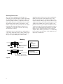
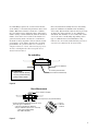
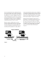
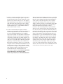
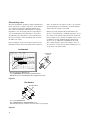
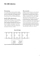
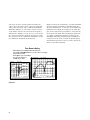
Agilent AN 1287-9
In-Fixture Measurements Using
Vector Network Analyzers
Application Note
Agilent Network Analysis Solutions
Table of Contents
3
3
4
4
5
5
6
7
8
12
13
13
13
15
16
17
17
17
17
18
18
19
19
20
20
22
25
30
32
2
Introduction
The need for fixtures
Measurement errors
Measurement calibration
Calibration kit
Standard definition
Standard class assignment
Fixtures for R&D versus manufacturing
Removing fixture errors
Characterizing calibration standards for SOLT calibration
Characterizing a short
Characterizing an open
How to determine open capacitance
Characterizing a load
Characterizing a thru
TRL/LRM calibration
TRL terminology
How TRL*/LRM* calibration works
TRL* error model
Isolation
Source match and load match
How true TRL/LRM works
(four-sampler receiver architecture only)
Improving raw source match and load match for
TRL*/LRM* calibration
The TRL calibration
Requirements for TRL standards
Fabricating and defining calibration standards for TRL/LRM
Using TDR to evaluate fixtures and standards
Biasing active parts
Conclusion
Introduction
This application note describes the use of vector
network analyzers when making measurements of
components in fixtures. We will explain the need
for fixtures, the selection of fixtures, measurement
error, how to minimize the errors, basic fixture
construction, and the construction and characterization of required calibration standards, if commercial fixtures are not available for your device.
The need for fixtures
Size, weight, and cost constraints along with higher
operating frequencies and advances in technology
are driving the use of smaller and more integrated
packaged parts at the assembly level. Now there
are many nonstandard surface-mount technology
(SMT) packages for many RF (<3 GHz) applications.
The physical dimensions of these parts vary greatly,
due to differing technologies, power-handling
requirements, environmental conditions, and
design criteria. With the wide variety of component sizes and shapes, no single fixture fits all.
Making quality RF measurements on devices with
standard coaxial connectors is relatively easy.
Very accurate measurements can be made using
commercial calibration kits and standard errorcorrection routines found in most network ana
lyzers. Devices without connectors are difficult to
measure since some sort of test fixture is required
to provide electrical and mechanical connection
between the device under test (DUT) and the coaxial-
connector-based test equipment. In addition,
in-fixture calibration standards are often required
to achieve the level of measurement accuracy
demanded by many of today’s devices.
An “ideal” fixture would provide a transparent
connection between the test instrument and the
device being tested. It would allow direct measurement of the DUT, without imposition of the fixture’s
characteristics. In parametric terms, this would
mean the fixture would have no loss, a flat frequency
response with linear phase, no mismatches, be a
precisely known electrical length, and have infinite
isolation between input and output (zero crosstalk).
If we could make such a fixture, calibration would
be unnecessary.
Since it is impossible to make an ideal fixture, we
can only approximate the ideal case. We need to
do this by optimizing the performance of the test
fixture relative to the performance of the DUT. We
can try to make the loss of the fixture smaller than
the specified gain or insertion loss uncertainty of
the DUT. The bandwidth of the fixture needs to be
wider than the desired measurement bandwidth of
the DUT. Mismatch can be minimized with good
design and the use of effective measurement tools
such as time-domain reflectometry (TDR) to identify
the mismatches in the fixture. The electrical length
of the fixture can be measured. Fixture crosstalk need
only be less than the isolation of the device under
test. Since we can only approximate the perfect
fixture, the type of calibration required for any
particular application will depend solely on how
stringent the DUT specifications are.
3
Measurement errors
Measurement calibration
Before we discuss calibration, we need to briefly
discuss what factors contribute to measurement
uncertainty.
A more complete definition of measurement
calibration using the network analyzer and a
description of error models are included in the
network analyzer operating manual. The basic
ideas are summarized here.
Errors in network analyzer measurements can be
separated into three categories:
Drift errors occur when the test system’s performance changes after a calibration has been performed.
They are primarily caused by temperature variation
and can be removed by recalibration.
Random errors vary as a function of time. Since
they are not predictable they cannot be removed
by calibration. The main contributors to random
errors are instrument noise, switch repeatability,
and connector repeatability. The best way to reduce
random errors is by decreasing the IF bandwidth,
or by using trace averaging over multiple sweeps.
Systematic errors include mismatch, leakage, and
system frequency response. In most microwave or
RF measurements, systematic errors are the most
significant source of measurement uncertainty.
The six systematic errors in the forward direction
are directivity, source match, reflection tracking,
load match, transmission tracking, and isolation.
The reverse error model is a mirror image, giving
a total of 12 errors for two-port measurements.
Calibration is the process for removing these
errors from network analyzer measurements.
4
Measurement calibration is a process in which
a network analyzer measures precisely known
devices and stores the vector differences between
the measured and the actual values. The error
data is used to remove the systematic errors from
subsequent measurements of unknown devices.
There are six types of calibrations available with
the vector network analyzer: response, response
and isolation, S11 1-PORT, S22 1-PORT, FULL
2-port, and TRL 2-PORT. Each of these calibration
types solves for a different set of systematic
measurement errors.
A RESPONSE calibration solves for the systematic
error term for reflection or transmission tracking,
depending on the S-parameter that is activated on
the network analyzer at the time of the calibration.
RESPONSE & ISOLATION adds correction for
crosstalk to a simple RESPONSE calibration. An
S11 1-PORT calibration solves for forward error
terms, directivity, source match, and reflection
tracking. Likewise, the S22 1-PORT calibration
solves for the same terms in the reverse. Full
2-PORT and TRL 2-PORT calibrations include forward and reverse error terms of both ports, plus
transmission tracking and isolation.
The type of measurement calibration selected by
the user depends on the device to be measured
(for example one-port or two-port device) and the
extent of accuracy enhancement desired. Further,
a combination of calibrations can be used in the
measurement of a particular device.
The accuracy of subsequent DUT measurements is
dependent on the accuracy of the test equipment,
how well the known devices are modeled, and the
exactness of the error correction model.
Calibration kit
Measurement accuracy is largely dependent upon
calibration standards, and a set of calibration
standards is often supplied as a calibration kit.
Each standard has precisely known or predictable
magnitude and phase response as a function of
frequency. For the network analyzer to use the
standards of a calibration kit, the response of each
standard must be mathematically defined and then
organized into a standard class that corresponds
to the error model used by the network analyzer.
Agilent Technologies currently supplies calibration
kits for most coaxial components. However, when
measuring non-coaxial components it is necessary
to create and define the standards that will be
used with the fixture.
Standard definition
The standard definition describes the electrical
characteristics (delay, attenuation, and impedance)
of each calibration standard. These electrical
characteristics can be derived mathematically
from the physical dimensions and material of each
calibration standard or from the actual measure
response. A Standard Definitions table (see Figure 1)
lists the parameters that are used by the network
analyzer to specify the mathematical model.
Figure 1.
5
Standard class assignment
The standard class assignment organizes calibration
standards into a format that is compatible with the
error models used in measurement calibration. A
class or group of classes corresponds to one of
seven calibration types used in the network analyzer.
A Standard Class Assignments table (see Figure 2)
Figure 2.
6
lists the class assignments for each standard type.
Agilent Application Note 1287-3, Applying Error
Correction to Network Analyzer Measurements,
will provide a more in-depth discussion of network
analyzer basics.
Fixtures for R&D versus manufacturing
Fixtures intended for manufacturing applications
look different than those used in R&D, since the
basic design goals are different. In manufacturing,
high throughput is the overriding concern. A fixture
that allows quick insertion, alignment and clamping
is needed. It must be rugged, since many thousands
of parts will be inserted in the fixture over its
lifetime. Fixtures designed for manufacturing use
tend to be mechanically sophisticated. For R&D
applications the fixtures can be much simpler and
less rugged. They can be PCB-based, and since we
are usually testing only a few devices, we can get
by with soldering parts in and out of the fixture.
Fixturing in R&D versus
Manufacturing
Manufacturing
R&D
• quick insertion, alignment, clamping
• rugged for high-volume use
• compliant contacts
• usually mechanically sophisticated
• solder parts onto fixture
• ruggedness not an issue for low volumes
• soldering handles leaded / leadless parts
• often simple (e.g., PCB with connectors)
Figure 3.
Typical PCB Fixture (with Cal Standards)
Load standard
Short standard
Contact to DUT
Open standard
Thru standard
Coaxial connectors
Launches / Transitions
Figure 4.
This is an example of a typical fixture used in
the R&D application. It incorporates calibration
standards and has a section where the DUT can
be attached.
7
Removing fixture errors
There are three fundamental techniques for
removing errors introduced by a fixture: modeling,
de-embedding, and direct measurement. Each has
relatively simple and more complicated versions
that require greater work but yield more accurate
measurements. The relative performance of the
fixture compared to the specifications of the DUT
being measured will determine what level of
calibration is required to meet the necessary
measurement accuracy.
Calibration based on modeling uses mathematical
corrections derived from an accurate model of the
fixture. Often, the fixture is measured as part of
the process of providing an accurate model.
Modeling requires that we have data regarding the
fixture characteristics. The simplest way to use
this data is with the port extension feature of the
network analyzer. First you perform a full two-port
calibration at the points indicated in Figure 5. This
calibration establishes the reference plane at the
junction of the test port cables. The fixture is then
connected to the test port cables and the reference
plane is then mathematically adjusted to the DUT,
using the port extension feature of the network
analyzer. If the fixture performance is considerably
better than the specifications of the DUT, this technique may be sufficient.
Modeling
Port extensions
Two-port calibration
Mathematically extend
reference plane
assume:
no loss
flat magnitude
linear phase
constant impedance
De-embedding
Two-port calibration
Accurate S-parameter data
(from model or measurement)
Figure 5.
8
external software required
De-embedding requires an accurate linear model
of the fixture, or measured S-parameter data of the
fixture. External software is needed to combine
the error data from a calibration done without the
fixture (using coaxial standards) with the modeled
fixture error. If the error terms of the fixture are
generated solely from a model, the overall measurement accuracy depends on how well the actual
performance of the fixture matches the modeled
performance. For fixtures that are not based on
simple transmission lines, determining a precise
model is usually harder than using the direct
measurement method.
Direct measurement usually involves measuring
physical calibration standards and calculating
error terms. This method is based on how precisely
we know the characteristics of our calibration
standards. The number of error terms that can be
corrected varies considerably depending on the
type of calibration used. Normalization only
removes one error term, while full two-port error
correction accounts for all 12 error terms.
De-embedding
DUT
Two-port calibration
Accurate S-parameter data
(from model or measurement)
De-embedding:
• requires external software
• accuracy is determined by
quality of fixture model
Figure 6.
Direct Measurement
Various calibration standards
DUT
Measurement plane (for cal standards and DUT)
• measure standards to determine systematic errors
• two major types of calibrations:
• response (normalization) calibration
• two-port calibration (vector-error correction)
Various
calibration
standards
• short-open-load-thru (SOLT)
• thru-reflect-line (TRL)
Figure 7.
9
Direct measurements have the advantage that the
precise characteristics of the fixture do not need to
be known beforehand. They are measured during
the calibration process. The simplest form of direct
measurement is a response calibration, which is a
form of normalization. A reference trace is placed
in memory and subsequent traces are displayed as
data divided by memory. A response calibration
only requires one standard each for transmission
(a thru) and reflection (a short or open).
However, response calibration has a serious
inherent weakness due to the lack of correction
for source and load mismatch and coupler/bridge
directivity. Mismatch is especially troublesome
for low-loss transmission measurements (such as
measuring a filter passband or a cable), and for
reflection measurements. Using response calibration
for transmission measurements on low-loss devices
can result in considerable measurement uncertainty
in the form of ripple. Measurement accuracy will
depend on the relative mismatch of the test fixture
in the network analyzer compared to the DUT.
When measuring transmission characteristics
with fixtures, considerable measurement accuracy
improvement can be obtained by performing a
two- port correction at the ends of test cables.
This calibration improves the effective source and
load match of the network analyzer, thus helping
to reduce the measurement ripple, the result of
reflec- tions from the fixture and analyzer’s
test ports.
Response Calibration
thru
DUT
Reference
errors due
to mismatch
Figure 8.
10
Measurement
Two-port calibration provides much more accurate
measurements compared to a response calibration.
It also requires more calibration standards. There
are two basic types of two-port calibration: ShortOpen-Load-Thru (SOLT) and the Thru-Reflect-Line
(TRL). These are named after the types of standards
used in the calibration process.
A calibration at the coaxial ports of the network
analyzer removes the effects of the network analyzer
and any cables or adapters before the fixture;
however, the effects of the fixture itself are not
accounted for. An in-fixture calibration is preferable, but high-quality SOLT standards are not readily available to allow a conventional full two-port
calibration of the system at the desired measurement plane of the device. In microstrip, a short
circuit is inductive, an open circuit radiates energy,
and a high-quality purely resistive load is difficult
to produce over a broad frequency range. The TRL
two-port calibration is an alternative to the traditional SOLT Full two-port calibration technique
that utilizes simpler, more convenient standards
for device measurements in the microstrip
environment.
In all measurement environments, the user must
provide calibration standards for the desired calibration to be performed. The advantage of TRL is
that only three standards need to be characterized
as opposed to four in the traditional SOLT full twoport calibrations. Further, the requirements for
characterizing the T, R, and L standards are less
stringent and these standards are more easily
fabricated.
For more information on network analyzer calibrations, please see Agilent Application Note 1287-3,
Applying Error Correction to Network Analyzer
Measurements.
Two-Port Calibration
Two-port calibration corrects for all major
sources of systematic measurement errors
R
A
B
Crosstalk
Directivity
DUT
Frequency response
reflection tracking (A/R)
transmission tracking (B/R)
Source
Mismatch
Load
Mismatch
Six forward and six reverse error terms
yields 12 error terms for two-port devices
Figure 9.
11
Characterizing calibration standards for
SOLT calibration
Most network analyzers already contain standard
calibration kit definition files that describe the
characteristics of a variety of calibration standards.
These calibration kit definitions usually cover
the major types of coaxial connectors used for
component and circuit measurements, for example
Type-N, 7 mm, 3.5 mm and 2.4 mm. Most high-performance network analyzers allow the user to
modify the definitions of the calibration standards.
This capability is especially important for fixturebased measurements, because the in-fixture calibration standards rarely have the same attributes
as the coaxial standards. Custom calibration
standards, such as those used with fixtures,require
the user to characterize the standards and enter
the definitions into the network analyzer. The
calibration kit definition must match the
actual standards for accurate measurements.
Definitions of the in-fixture calibration standards
can be stored in the analyzer as a custom userdefined calibration kit.
While there are many characteristics used to
describe calibration standards, only a few need to
be modified for most fixture applications. For a
properly designed PCB fixture, only the fringing
capacitance of the open standard and the delay of
the short need to be characterized.
Short-Open-Load-Thru (SOLT)
Calibration
SOLT calibration is attractive for RF fixtures
• simpler and less-expensive fixtures and standards
• relatively easy to make broadband calibration standards
• short, thru are easiest
• open requires characterization
• load is hardest (quality determines corrected directivity)
Figure 10.
12
open
thru
short
load
Characterizing a short
The electrical definition of an ideal short is unity
reflection with 180 degrees of phase shift. All of
the incident energy is reflected back to the source,
perfectly out of phase with the reference. A simple
short circuit from a single conductor to ground
makes a good short standard. For example, the
short can be a few vias (plated through holes) to
ground at the end of a micro-strip transmission
line. If coplanar transmission lines are used, the
short should go to both ground planes.
To reduce the inductance of the short, avoid
excessive length. A good RF ground should be
near the signal trace. If the short is not exactly at
the contact plane of the DUT, an offset length can
be entered (in terms of electrical delay) as part of
the user-defined calibration kit.
Characterizing an open
The open standard is typically realized as an unterminated transmission line. Electrical definition of
an ideal open has “unity reflection with no phaseshift.” The actual model for the open, however, does
have some phase shift due to fringing capacitance.
How to determine open capacitance
Determining the fringing capacitance is only
necessary above approximately 300 MHz. The
fringing capacitance can be measured as follows:
1. Perform a one-port calibration at the end of the
test cable. Use a connector type that is compatible with the fixture. For example, use APC 3.5-mm
standards for a fixture using SMA connectors.
2. Connect the fixture and measure the load standard. This data should be stored in memory and
the display changed to “data minus memory.” This
step subtracts out the reflection of the fixture
connector (assuming good consistency between
connectors), so that we can characterize just
the open. (An alternative is to use time-domain
gating to remove the effect of the connector.)
Determining Open Capacitance
• perform one-port calibration
at end of test cable
• measure load, store data in
memory, display data-mem
• measure short, add port
extension until flat 180° phase
• measure open, read capacitance
from admittance Smith chart
• enter capacitance coefficient(s)
in cal-kit definition of open
1: 228.23 uS 1.2453 mS 209.29 fF 947.000
CH1 S22 1 U FS MHz
PRm
Cor
Del
1
START .050 000 000
GHz
STOP 6.000 000 000
GHz
watch out for "negative" capacitance (due to long or inductive short)
adjust with negative offset-delay in open <or>
positive offset-delay in short
Figure 11.
13
3. Measure the short standard. Set the port extension to get a flat 180 degrees phase response.
To fine-tune the value of port extension, set the
phase-off set value for the trace to 180 degrees
and expand degrees-per-division scale. Mismatch
and directivity reflections may cause a slight
ripple, so use your best judgment for determining the flattest trace, or use marker statistics
(set the mean value to zero).
4. Set the network analyzer display format to
Smith chart, the marker function to Smith chart
format G+jB (admittance) and then measure
the open standard. Markers now read G+jB
instead of the R+jX of an impedance Smith chart.
Admittance must be used because the fringing
capacitance is modeled as a shunt element, not
a series element. The fringing capacitance (typically 0.03 to 0.25 pF) can be directly read at the
frequency of interest using a trace marker. At
RF, a single capacitance value (Co) is generally
adequate for the calibration kit definition of the
open. In some cases, a single capacitance number may not be adequate, as capacitance can vary
with frequency. This is typically true for the
measurements that extend well into the
microwave frequency range. Because capacitance
varies with frequency, at frequencies above
3 GHz it may be better to use a TRL/LRM calibration.
14
When measuring the fringing capacitance, a problem
can arise if the short standard is electrically longer
than the open standard. The measured impedance
of the open circuit then appears to be a negative
capacitor, indicated by a trace that rotates backwards (counter-clockwise) on the Smith chart. This
problem is a result of using an electrically longer
short standard as the 180 degrees phase
reference. The electrically shorter open will then
appear to have positive phase. The remedy for this
is to decrease the port extension until the phase is
monotonically negative. The model for the open will
then have a normal (positive) capacitance value. The
value of the negative offset delay that needs to be
included in the open standard definition is simply
the amount by which port extension was reduced
(for instance, the difference in the port extension
values between the short and the open). In effect,
we have now set the reference plane at the short.
Alternatively, the offset delay of the open can be
set to zero, and a small positive offset delay can be
added to the model of the short standard. This will
set an effective reference plane at the open.
Characterizing a load
An ideal load reflects none of the incident signal,
thereby providing a perfect termination over a
broad frequency range. We can only approximate
an ideal load with a real termination because some
reflection always occurs at some frequency,
especially with non-coaxial actual standards.
At RF, we can build a good load using standard
surface-mount resistors. Usually, it is better to
use two 100-ohm resistors in parallel instead of
a single 50-ohm resistor, because the parasitic
inductance is cut in half. For example, 0805-size
SMT resistors have about 1.2 nH series inductance
and 0.2 pF parallel capacitance. Two parallel
100-ohm 0805 resistors have nearly a 20-dB better
match than a single 50-ohm resistor.
Port Extensions
• port-extension feature of network analyzer
removes linear portion of phase response
• accounts for added electrical length of fixture
• doesn't correct for loss or mismatch
• mismatch can occur from
• launches
• variations in transmission line impedance
After port extensions
applied, fixture phase
response is flat
Frequency
Phase 45 o /Div
Fixture response without
port extensions
Frequency
Figure 12.
15
Characterizing a thru
The thru standard is usually a simple transmission
line between two coaxial connectors on the fixture.
A good thru should have minimal mismatch at
the connector launches and maintain a constant
impedance over its length (which is generally the
case for PCB thrus). The impedance of the thru
should match the impedance of the transmission
lines used with the other standards (all of which
should be 50 ohms).
Since we want the two halves of line to be equal in
electrical length to the thru line, the PCB must be
widened by the length of the DUT.
With a properly designed PC board fixture, the
short (or open) defines a calibration plane to be in
the center of the fixture. This means the thru will
have a length of zero (which is usually not the case
for fixtures used in manufacturing applications,
where a set of calibration standards is inserted
into a single fixture). Since the length is zero, we
do not have to worry about characterizing the loss
of the thru or its phase shift.
Notice in Figure 12, the PC board is wider for the
transmission line where the DUT will be soldered.
Load Standard
CH1 S11
CH2 MEM
log MAG
5 dB/
5 dB/
REF 0 dB
REF 0 dB
two 100-ohm
resistors
PRm
Cor
One 50-ohm SMT resistor
1: -24.229 dB 1 GHz
2: -14.792 dB 3 GHz
2
1
Two 100-ohm SMT resistors
PRm
Cor
1
2
2
1: -41.908 dB 1 GHz
2: -32.541 dB 3 GHz
1
STOP 6 000.000 000 MHz
START .300 000 MHz
• ideal: zero reflection at all frequencies
• can only approximate at best (usually somewhat inductive)
• two 100-ohm resistors in parallel better than a single 50-ohm resistor
Figure 13.
Thru Standard
DUT placed here
thru
• thru is a simple transmission line
• desire constant impedance and minimal mismatch at ends
• PCB is widened by the length of the DUT to insure that both lines are of equal length
Figure 14.
16
TRL/LRM Calibration
TRL terminology
TRL* error maodel
Notice that the letters TRL, LRL, LRM, and TRM
are often interchanged, depending on the standards
used. For example, “LRL” indicates that two lines
and a reflect standard are used; “TRM” indicates
that a thru, reflection, and match standards are
used. All of these refer to the same basic method.
For TRL* two-port calibration, a total of 10 measurements are made to quantify eight unknowns
(not including the two isolation error terms).
Assume the two transmission leakage terms, EXF
and EXR, are measured using the conventional
technique. Although this error model is slightly
different from the traditional Full two-port
12-term model, the conventional error terms may
be derived from it. For example, the forward
reflection tracking (ERF) is represented by the
product of ε10 and ε01. Also notice that the forward
source match (ESF) and reverse load match (ELR)
are both represented by ε11, while the reverse
source match (ESR) and forward load match (ELF)
are both represented by ε22. In order to solve for
these eight unknown TRL* error terms, eight linearly independent equations are required.
How TRL*/LRM* calibration works
The TRL*/LRM* calibration is used in a network
analyzer with a three-sampler receiver architecture,
and relies on the characteristic impedance of
simple transmission lines rather than on a set of
discrete impedance standards. Since transmission
lines are relatively easy to fabricate (in a microstrip, for example), the impedance of these lines
can be determined from the physical dimensions
and substrate’s dielectric constant.
8 Term TRL* Model
Figure 15. 8-term TRL* error model and generalized coefficients
17
Isolation
The first step in the TRL* two-port calibration
process is the same as the transmission step for a
full two-port calibration. For the thru step, the test
ports are connected together directly (zero length
thru) or with a short length of transmission line
(non- zero length thru) and the transmission frequency response and port match are measured in
both directions by measuring all four S-parameters.
For the reflect step, identical high reflection
coefficient standards (typically open or short
circuits) are connected to each test port and
measured (S11 and S22).
For the line step, a short length of transmission
line (different in length from the thru) is inserted
between port I and port 2 and again the frequency
response and port match are measured in both
directions by measuring all four S-parameters.
In total, 10 measurements are made, resulting in
10 independent equations. However, the TRL* error
model has only eight error terms to solve for. The
characteristic impedance of the line standard
becomes the measurement reference and, therefore,
has to be assumed ideal (or known and defined
precisely).
At this point, the forward and reverse directivity
(EDF and EDR), transmission tracking (ETF and ETR),
and reflection tracking (ERF and ERR) terms may be
derived from the TRL* error terms. This leaves the
isolation (EXF and EXR), source match (ESF and ESR)
and load match (ELF and ELR) terms to discuss.
18
Two additional measurements are required to
solve for the isolation terms (EXF and EXR).
Isolation is characterized in the same manner
as the full two-port calibration. Forward and
reverse isolation are measured as the leakage
(or crosstalk) from port 1 to port 2 with each port
terminated. The isolation part of the calibration is
generally only necessary when measuring high-loss
devices (greater than 70 dB).
Note: If an isolation calibration is performed,
the fixture leakage must be the same during the
isolation calibration and the measurement.
Source match and load match
A TRL* calibration assumes a perfectly balanced
test set architecture as shown by the ε11 term,
which represents both the forward source match
(ESF) and reverse load match (ELR), and by the ε22
term, which represents both the reverse source
match (ESR) and forward load match (ELF). However,
in any switching test set, the source and load
match terms are not equal because the transfer
switch presents a different terminating impedance
as it is changed between port 1 and port 2.
For network analyzers that are based on a threesampler receiver architecture, it is not possible to
differentiate the source match from the load match
terms. The terminating impedance of the switch
is assumed to be the same in either direction.
Therefore, the test port mismatch cannot be fully
corrected. An assumption is made that:
forward source match (ESF) = reverse load match
(ELR) = ε11
reverse source match (ESR) = forward load match
(ELF) = ε22
For a fixture, TRL* can eliminate the effects of the
fixture’s loss and length, but does not completely
remove the effects due to the mismatch of the
fixture. This is in contrast to the “pure” TRL
technique used by instruments equipped with
four-sampler receiver architecture.
Note: Because the TRL technique relies on the
characteristic impedance of transmission lines, the
mathematically equivalent method LRM* (for linereflect-match) may be substituted for TRL*. Since
a well-matched termination is, in essence, an
infinitely long transmission line, it is well-suited
for low (RF) frequency calibrations. Achieving a
long line standard for low frequencies is often
physically impossible.
How true TRL/LRM works
(four-sampler receiver architecture only)
The TRL implementation with four-sampler receiver
architecture requires a total of 14 measurements
to quantify 10 unknowns, as opposed to only a
total of 12 measurements for TRL*. (Both include
the two isolation error terms.)
Because of the four-sampler receiver architecture,
additional correction of the source match and load
match terms is achieved by measuring the ratio of
the two “reference” receivers during the thru and
line steps. These measurements characterize the
impedance of the switch and associated hardware
in both the forward and reverse measurement
configurations. They are then used to modify the
corresponding source and load match terms (for
both forward and reverse).
The four-sampler receiver architecture configuration with TRL establishes a higher performance
calibration method over TRL* when making in-fixture measurements, because all significant error
terms are systematically reduced. With TRL*, the
source and load match terms are essentially those
of the raw, “uncorrected” performance of the hardware.
Improving raw source match and load match
for TRL*/LRM* calibration
A technique that can be used to improve the raw
test port mismatch is to add high-quality fixed
attenuators as closely as possible to the measurement plane. The effective match of the system is
improved because the fixed attenuators usually
have a return loss that is better than that of the
network analyzer. Additionally, the attenuators
provide some isolation of reflected signals. The
attenuators also help to minimize the difference
between the port source match and load match,
making the error terms more equivalent.
With the attenuators in place, the effective port
match of the system is improved so that the
mismatch of the fixture transition itself dominates
the measurement errors after a calibration.
19
The TRL Calibration
Requirements for TRL standards
If the device requires bias, it will be necessary to
add external bias tees between the fixed attenuators and the fixture. The internal bias tees of the
analyzer will not pass the bias properly through
the external fixed attenuators. Be sure to calibrate
with the external bias tees in place (no bias
applied during calibration) to remove their
effects from the measurement.
Because the bias tees must be placed after the
attenuators, they essentially become part of the
fixture. Therefore, their mismatch effects on the measurement will not be improved by the attenuators.
Although the fixed attenuators improve the raw
mismatch of the network analyzer system, they
also degrade the overall measurement dynamic
range.
This effective mismatch of the system after
calibration has the biggest effect on reflection
measurements of highly reflective devices.
Likewise, for well-matched devices, the effects
of mismatch are negligible. This can be shown
by the following approximation:
Reflection magnitude uncertainty = ED + ERS11
+ ES(S11)2 + ELS21SI2
Transmission magnitude uncertainty = EX + ETS21
+ ESS11S21 + ELS22S21
where:
ED = effective directivity
ER = effective reflection tracking
ES = effective source match
EL = effective load match
Ex = effective crosstalk
ET = effective transmission tracking
Sxx = S-parameters of the device under test
20
When building a set of TRL standards for a microstrip or fixture environment, the requirements for
each of these standard types must be satisfied.
Types
Requirements
THRU
(Zero length)
No loss. Characteristic impedance
(Z0 ) need not be known.
S21 = S11= 1 ∠ 0°
S11 = S22 = 0
THRU
(Non-zero
length)
Z0 of the thru must be the same as
the line (if they are not the same,
the average impedance is used).
Attenuation of the thru need not
be known.
If the thru is used to set the
reference plane, the insertion phase
or electrical length must be wellknown and specified. If a non-zero
length thru is specified to have zero
delay, the reference plane is established in the middle of the thru.
Types
Requirements (continued)
REFLECT
Reflection coefficient (Γ) magnitude
is optimally 1.0, but need not be
known.
Phase of Γ must known and specified
to within ± 1/4 wavelength or ± 90°.
During computation of the error
model, the root choice in the solution
of a quadratic equation is based on
the reflection data. An error in definition would show up as a 180° error
in the measured phase. Γ must be
identical on both ports. If the reflect
is used to set the reference plane, the
phase response must be well-known
and specified.
LINE/MATCH Z0 of the line establishes the refer(LINE)
ence impedance of the measurement
(i.e. S11 = S22 = 0). The calibration
impedance is defined to be the same
as Z0 of the line. If the Z0 is known
but not the desired value (i.e., not
equal to 50 Ω), the SYSTEMS Z0
selection under the TRL/LRM options
menu is used.
Insertion phase of the line must not
be the same as the thru (zero length
or non-zero length). The difference
between the thru and line must be
between (20° and 160°) ± n x 180°.
Measurement uncertainty will increase
significantly when the insertion phase
nears 0 or an integer multiple of 180°.
Optimal line length is 1/4 wavelength
or 90° of insertion phase relative to
the thru at the middle of the desired
frequency span.
Usable bandwidth for a single thru/
line pair is 8:1 (frequency span:start
frequency).
Multiple thru/line pairs (Z0 assumed
identical) can be used to extend the
bandwidth to the extent transmission
lines are available.
Attenuation of the line need not be
known.
Insertion phase must be known and
specified within ± 1/4 wavelength or
± 90°.
LINE/MATCH Z0 of the match establishes the refer(MATCH)
ence impedance of the measurement.
Γ must be identical on both ports.
21
Fabricating and defining calibration
standards for TRL/LRM
When calibrating a network analyzer, the actual
calibration standards must have known physical
characteristics. For the reflect standard, these
characteristics include the offset in electrical delay
(seconds) and the loss (ohms/second of delay). The
characteristic impedance, OFFSET = Z0, is not used
in the calculations because it is determined by the
line standard. The reflection coefficient magnitude
should optimally be 1.0, but need not be known
since the same reflection coefficient magnitude
must be applied to both ports.
The thru standard may be a zero-length or known
length of transmission line. The value of length
must be converted to electrical delay, just as for
the reflect standard. The loss term must also be
specified.
±N x 180 degrees where N is an integer.) If two
lines are used (LRL), the difference in electrical
length of the two lines should meet these optimal
conditions. Measurement uncertainty will increase
significantly when the insertion phase nears zero
or is an integer multiple of 180 degrees, and this
condition is not recommended.
For a transmission media that exhibits linear phase
over the frequency range of interest, the following
expression can be used to determine a suitable line
length of 1/4 wavelength at the center frequency
(which equals the sum of the start frequency and
stop frequency divided by 2):
Electrical length (cm) = (LINE – 0 length THRU)
Electrical length (cm) =
The line standard must meet specific frequencyrelated criteria, in conjunction with the length
used by the thru standard. In particular, the insertion phase of the line must not be the same as the
thru. The optimal line length is 1/4 wavelength (90
degrees) relative to a zero length thru at the center
frequency of interest, and between 20 and 160
degrees of phase difference over the frequency
range of interest. (Note: these phase values can be
22
(15000 x VF)
f1(MHz) + f2(MHz)
let:
f1 = 1000 MHz
f2 = 2000 MHz
VF = Velocity Factor = 1 (for this example)
Thus, the length to initially check is 5 cm.
Next, use the following to verify the insertion
phase at f1 and f2:
Phase (degrees) = (360 x f x l)
v
where:
f = frequency
l = length of line
v = velocity = speed of light x velocity factor
which can be reduced to the following, using frequencies in MHz and length in centimeters:
Phase (degrees) approx. = 0.012 x f(MHz) x l(cm)
VF
So for an air line (velocity factor approximately 1)
at 1000 MHz, the insertion phase is 60 degrees for
a 5-cm line; it is 120 degrees at 2000 MHz. This line
would be a suitable line standard.
For microstrip and other fabricated standards, the
velocity factor is significant. In those cases, the
phase calculation must be divided by that factor.
For example, if the dielectric constant for a sub-
strate is 10, and the corresponding “effective”
dielectric constant for microstrip is 6.5, then the
“effective” velocity factor equals 0.39 (1 ÷ square
root of 6.5).
Using the first equation with a velocity factor of
0.39, the initial length to test would be 1.95 cm.
This length provides an insertion phase at 1000 MHz
of 60 degrees; at 2000 MHz, 120 degrees (the insertion phase should be the same as the air line
because the velocity factor was accounted for
when using the first equation).
Another reason for showing this example is to
point out the potential problem in calibrating at
low frequencies using TRL. For example, 1/4 wavelength is:
Length (cm) =
7500 x VF
fc
where:
fc = center frequency
Thus, at 50 MHz:
Length (cm) = 7500 = 150 cm or 1.5 m
50 (MHz)
23
Such a line standard would not only be difficult to
fabricate, but its long term stability and usability
would be questionable as well.
either be of zero length or non-zero length. The
same rules for thru and reflect standards used for
TRL apply for TRM.
Thus at lower frequencies and/or very broad band
measurements, fabrication of a “match” or termination may be deemed more practical. Since a termination is, in essence, an infinitely long transmission line, it fits the TRL model mathematically, and
is sometimes referred to as a “TRM” calibration.
TRM has no inherent frequency coverage limitations which makes it more convenient in some
measurement situations. Additionally, because TRL
requires a different physical length for the thru
and the line standards, its use becomes impractical
for fixtures with contacts that are at a fixed
physical distance from each other.
The TRM calibration technique is related to TRL
with the difference being that it bases the characteristic impedance of the measurement on a
matched Z0 termination instead of a transmission
line for the third measurement standard. Like the
TRL thru standard, the TRM THRU standard can
24
For more information on how to modify calibration
constants for TRL/LRM, and how to perform a TRL
or LRM calibration, refer to the “Optimizing
Measurement Results” in the network analyzer
user’s manual.
Using TDR to evaluate fixtures and standards
Using TDR to Evaluate Fixture and Standards
Time-domain reflectometry (TDR) is a helpful tool.
We can distinguish between capacitive and inductive mismatches, and see non-Z0 transmission
lines. TDR can help us determine the magnitude
of and distance to reflections of the fixture and
the calibration standards. Once the fixture has
been designed and fabricated, we can use TDR to
effectively evaluate how well we have minimized
reflections.
impedance
• what is TDR?
• time-domain reflectometry
• analyze impedance versus time
• distinguish between inductive and capacitive transitions
• with gating:
• analyze transitions
• analyzer standards
inductive
transition
Zo
time
capacitive
transition
TDR measurements using a vector network analyzer
start with a broadband sweep in the frequency
domain. The inverse-Fourier transform is used to
transform the frequency-domain data to the timedomain, yielding TDR measurements. The spatial
resolution is inversely proportional to the frequency
span of the measurement. The wider the frequency
span, the smaller the distance that can be resolved.
For this reason, it is generally necessary to make
microwave measurements on the fixture to get
sufficient resolution for analyzing the various
transmissions.
non-Zo transmission line
Figure 16.
TDR Basics Using a Network Analyzer
• start with broadband frequency sweep
(often requires microwave VNA)
• inverse FFT to compute time-domain
• resolution inversely proportionate to
frequency span
CH1 S 22 Re
Cor
50 mU/ REF 0 U
20 GHz
6 GHz
CH1 START 0 s
STOP 1.5 ns
Figure 17.
For example, it may be necessary to measure a fixture
designed for use at 3 GHz with a frequency span of 0.05 GHz
to 20 GHz or even 40 GHz to get the needed resolution.
25
As long as we have enough spatial resolution we
can see the reflections of the connector independently of the reflections of the calibration standards.
With time-domain, we can isolate various sections
of the fixture and see the effects in the frequency
domain. For example, we can choose to look at just
the connector launches (without interference from
the reflections of the calibration standards), or just
the calibration standards by themselves.
Figure 18 shows the performance of a thru standard
used in a fixture intended for manufacturing use.
The time-domain plot, on the left, shows significant
mismatch at the input and output of the thru. The
plot on the right shows performance of the thru in
the frequency domain with and without gating. We
see about a 7-dB improvement in return loss (at
947 MHz) using time-domain gating, resulting in a
return loss for the thru of about 45 dB. The gated
measurement provides a more accurate characterization of the thru standard.
Time-Domain Gating
• TDR and gating can remove undesired reflections
only useful for broadband devices (a load or thru for example)
and broadband fixture
• define gate to only include DUT
• use two-port calibration
CH1 S11&Mlog MAG
5 dB/ REF 0 dB
at ends of test cables
PRm
Cor
CH1 MEM Re
PRm
Cor RISE TIME
29.994 ps
8.992 mm
20 mU/ REF 0 U
2
1: 48.729 mU 638 ps
2: 24.961 mU 668 ps
Gate
1: -45.113 dB 0.947 GHz
2: -15.78 dB 6.000 GHz
3: -10.891 mU 721 ps
1
2
3
thru in time domain
1
CH1 START 0 s
Figure 18.
26
STOP 1.5 ns
thru in frequency domain,
with and without gating
START .050 000 000 GHz
STOP 20.050 000 000 GHz
Time-domain gating can be a very useful tool for
evaluating how well the load is performing. We can
gate out the response of the fixture and just look at
the reflections due to the load standard, provided
we can get enough spatial resolution (this may
require the use of microwave vector network analyzers). The smoother trace on the plot on the left
shows the gated response of a load standard, with
a fairly typical match of about 38 dB at 1 GHz, and
around 30 dB at 2 GHz. The right-hand plot shows
that the load standard looks somewhat inductive,
which is fairly typical.
It is possible to adjust our load standard to compensate for the unavoidable parasitic characteristics that degrade the reflection response. Timedomain gating is an excellent tool for helping to
determine the proper compensation. For example,
we see the effect in both the time and the frequency
domains of adding a small capacitance to cancel
out some of the inductance of the load standard.
Characterizing and Adjusting Load
CH1 S 11&M log MAG 5 dB/ REF 0 dB
PRm
C
Gate
1: -38.805 dB 947 MHz
load mismatch
due to inductance
load in frequency domain,
with and without gating
CH1S11 Re
PRm
Cor
1
100 mU/REF 0 U
2
1: -61.951 mU 707 ps
2: 159.74 mU 749 ps
1
START .050 GHz
STOP 6.000 GHz
START .5 ns
• use time-domain gating to see load
reflections independent from fixture
• use time domain to compensate for imperfect load
(e.g. try to cancel out inductance)
STOP 1.5 ns
Figure 19.
27
When using PCB-based fixtures, performance at
the connector transition is important, and the consistency between connectors is critical. To minimize the effect of connector mismatch when using
multiple connectors on a fixture (a pair for each
calibration standard), there must be consistency
between the connectors and their mechanical
attachments to the fixture. Time-domain measurements are useful for analyzing both connector performance and repeatability; see Figure 21. For
information on making time-domain measurements
and using the gating feature, please see your network analyzer user’s guide.
Connectors on Fixtures
• transition at the connector launch causes reflection due to mismatch
• when cal standards are inserted in fixture, connector match is removed
• when each cal standard has connectors, consistency is very important
gap
Figure 20.
28
Connector Performance
CH1 S11
log MAG
10 dB/
REF 0 dB
PRm
Cor
CH1 START .099 751 243 GHz
CH2 S11
Re
frequency domain
edge connector
with gap
edge connector
Gat
PRm
Cor
1.900 GHz
1_: -23.753 dB
1_: -32.297 dB
right-angle
connector
STOP 20.049 999 843 GHz
50 mU/ REF 0 U
1_ -996 mU
right-angle
connector
edge connector
with gap
Comparing match
of right-angle and
edge-mount connectors
(with and without gap)
time domain
edge connector
CH2 START-500 ps
STOP 1 ns
Figure 21.
Connector Consistency
CH1 S11 -M log MAG
PRm
5 dB/
REF -10 dB
1.900 GHz
1_:-33.392 dB
1_ -43.278 dB
right-angle
connector
Cor
1
frequency domain
Gat
1
edge connector
CH1 START .099 751 243 GHz
CH2 S11 -M Re
STOP 20.049 999 843 GHz
49.6 mU/
REF 50 mU
1_ -8.0261 mU
Use [data - memory]
to check consistency
of connectors
PRm
Cor
1
edge connector
time domain
Gat
right-angle
connector
CH2 START-500 ps
STOP 1 ns
Figure 22.
29
Biasing active parts
Making in-fixture measurements of active parts
requires that DC bias be supplied along with the
RF signal. Traditionally, when bias was needed for
testing transistors, external bias tees were used
in the main RF signal paths. This approach is still
valid today although internal bias tees are provided
by most vector network analyzers.
Many packaged amplifiers and RFICs require that
DC power be supplied on separate pins. This means
that the fixture must provide extra connectors, DC
feedthroughs, wires, or pins for the necessary bias.
These bias connections should present a low DC
impedance. Discrete elements can be placed directly
on the fixture near the DUT to provide proper RF
bypassing and isolation of the DC supply pins. Good
RF bypassing techniques can be essential, as some
amplifiers will oscillate if RF signals couple onto
the supply lines.
Biasing Active Parts
DC Bias
RF
DUT
• can use bias-tees if RF and DC share same line
(many network analyzers contain internal bias tees)
• if separate, fixture needs extra connectors, pins or wires
• proper bypassing is important to prevent oscillation
Figure 23.
30
This is an example of how bias could be supplied
to a transistor. The power supplies are not shown,
but they would be connected to the +V base and
the +V collector nodes. The +V base controls the
collector current, and +V collector controls the
collector-to-emitter voltage on the transistor. For
the base resistors, it is important to use a fairly
large value (such as a 10K ohms), so that the voltage adjustment is not too sensitive. You may find it
convenient to use two digital voltmeters to monitor
the collector current and collector-to-emitter
voltage simultaneously.
Transistor Bias Example
to port-two
bias tee
to port-one
bias tee
50 MHz-20GHz
NETWORK ANALYZER
ACTIVE CHANNEL
Rbase
+Vbase
ENTRY
Rcollector
RESPONSE
(100 Ω)
(10K Ω)
STIMULUS
INSTRUMENT STATE
R
L
T
R CHANNEL
Collector-current
monitor
+Vcollector
S
HP-IB STATUS
PORT 1
PORT 2
5.07 V
7.53 V
Two-port calibration was performed prior
to taking S-parameter data of the transistor.
Collector-voltage
monitor
Figure 24.
31
www.agilent.com
Conclusion
We have covered the principles of in-fixture testing
of components with vector network analyzers. It is
time to determine the source of the fixture. Is the
fixture available commercially or must it be designed
and built? Inter-Continental Microwave is an Agilent
Channel Partner experienced in designing and
manufacturing test fixtures that are compatible
with Agilent network analyzers.
Inter-Continental Microwave contact information:
Inter-Continental Microwave
1515 Wyatt Drive
Santa Clara, CA 95054-1586
Tel: (408) 727-1596
Fax: (408) 727-0105
Fax-on-Demand: (408) 727-2763
Internet: www.icmicrowave.com
If it is necessary to design and build the fixture,
more information on calibration kit coefficient
modification can be found in the appropriate network analyzer user’s manual. A shareware program
that simplifies the process of modifying calibration
kit coefficients is available at www.vnahelp.com.
Agilent Technologies’ Test and Measurement Support, Services, and Assistance
Agilent Technologies aims to maximize the value you receive, while minimizing your
risk and problems. We strive to ensure that you get the test and measurement
capabilities you paid for and obtain the support you need. Our extensive support
resources and services can help you choose the right Agilent products for your
applications and apply them successfully. Every instrument and system we sell
has a global warranty. Two concepts underlie Agilent’s overall support policy: “Our
Promise” and “Your Advantage.”
Our Promise
Our Promise means your Agilent test and measurement equipment will meet
its advertised performance and functionality. When you are choosing new
equipment, we will help you with product information, including realistic performance specifications and practical recommendations from experienced test engineers. When you receive your new Agilent equipment, we can help verify that it
works properly and help with initial product operation.
Your Advantage
Your Advantage means that Agilent offers a wide range of additional expert test
and measurement services, which you can purchase according to your unique technical and business needs. Solve problems efficiently and gain a competitive edge
by contracting with us for calibration, extra-cost upgrades, out-of-warranty repairs,
and onsite education and training, as well as design, system integration, project
management, and other professional engineering services. Experienced Agilent
engineers and technicians worldwide can help you maximize your productivity, optimize the return on investment of your Agilent instruments and systems, and obtain
dependable measurement accuracy for the life of those products.
Agilent Open
www.agilent.com/find/open
Agilent Open simplifies the process of connecting and programming test systems
to help engineers design, validate and manufacture electronic products. Agilent
offers open connectivity for a broad range of system-ready instruments, open
industry software, PC-standard I/O and global support, which are combined to
more easily integrate test system development.
United States:
(tel) 800 829 4444
(fax) 800 829 4433
Canada:
(tel) 877 894 4414
(fax) 800 746 4866
China:
(tel) 800 810 0189
(fax) 800 820 2816
Europe:
(tel) 31 20 547 2111
Japan:
(tel) (81) 426 56 7832
(fax) (81) 426 56 7840
Agilent Email Updates
www.agilent.com/find/emailupdates
Get the latest information on the products and applications you select.
Korea:
(tel) (080) 769 0800
(fax) (080)769 0900
Latin America:
(tel) (305) 269 7500
Taiwan:
(tel) 0800 047 866
(fax) 0800 286 331
Other Asia Pacific
Countries:
(tel) (65) 6375 8100
(fax) (65) 6755 0042
Email: [email protected]
Contacts revised: 05/27/05
For more information on Agilent Technologies’ products, applications or services,
please contact your local Agilent office. The complete list is available at:
www.agilent.com/find/contactus
Product specifications and descriptions in this document subject to change
without notice.
Agilent Direct
www.agilent.com/find/agilentdirect
Quickly choose and use your test equipment solutions with confidence.
© Agilent Technologies, Inc. 1999, 2000, 2006
Printed in USA, January 10, 2006
5968-5329E