1
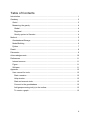
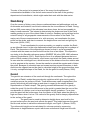
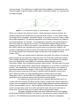
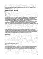
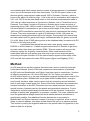
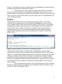
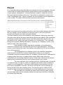
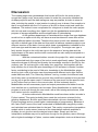
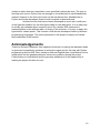
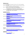
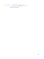
Introducing Lantmäteriet’s gravity data in ArcGIS with implementation of customized GIS functions Mattias Ryttberg Gravity is measured and used by Lantmäteriet to calculate a model of the geoid to get accurate reference heights for positioning. Lantmäteriet are continuously measuring new gravity and height data across Sweden to both complement, replace and to add new data points. This is mainly done by measurements in the field at benchmark points. One of the major reasons for continued measurements on e.g. benchmark points is that the measuring always moves forward which makes the measurements more accurate. More accurate data leads to a more accurate calculation of the geoid due to the more accurate gravity values. A more accurate geoid gives the possibility of more precise positioning across Sweden, due to the more precise height values. Lantmäteriet is in the process of updating their entire database of gravity data. They are also measuring at locations where there are none or sparse with measurements. As a stage in the renewing of their database and other systems the Geodesy department wishes to get an introduction to the ArcGIS environment. By customizations of several ArcGIS functions, Lantmäteriet’s work with the extensive data will get easier and perhaps faster. Customized tools will help make e. g. adding and removing data points easier, as well as making cross validation and several other functions only a click of a button away. Uppsala universitet, Institutionen för geovetenskaper Kandidatexamen i Geovetenskap, 180 hp Självständigt arbete i geovetenskap, 15 hp Tryckt hos Institutionen för geovetenskaper Geotryckeriet, Uppsala universitet, Uppsala, 2013. Självständigt arbete Nr 56 Introducing Lantmäteriet’s gravity data in ArcGIS with implementation of customized GIS functions Mattias Ryttberg Självständigt arbete Nr 56 Introducing Lantmäteriet’s gravity data in ArcGIS with implementation of customized GIS functions Mattias Ryttberg Handledare: Rickard Pettersson Sammanfattning Tyngdkraftsvärden mäts och används av Lantmäteriet för att beräkna en geoid som används för att få noggrann referenshöjd för positionering. Lantmäteriet uppdaterar hela tiden sin databas över tyngdkrafts- och höjddata. Detta för att lägga till, komplettera eller helt ersätta punkter med data. Den största delen av deras mätningar görs i fält på fixpunkter. En av de största anledningarna till att Lantmäteriet fortsätter att mäta på t.ex. gamla fixpunkter är att mätteknologin hela tiden går framåt, vilket leder till bättre mätningar. Mer precis data leder i sin tur till en bättre uträkning av geoiden på grund av mer korrekt tyngdkraftsdata. En mer precis geoid ger möjligheten för en mer precis positionering runtom i Sverige, detta på grund av den ökade säkerheten i höjdbestämningen. Lantmäteriet håller för närvarande på med att uppdatera hela sin databas över mätta punkter I Sverige. De håller också på med att mäta nya punkter där det inte finns några mätningar alls eller där de är få av dem. Som ett led i deras förnyelse av databasen och andra system vill geodesi avdelningen få en introduktion av ArcGIS miljön. Genom att modifiera flera olika funktioner i ArcGIS kan Lantmäteriets arbete med den stora databasen bli enklare och kanske snabbare. Modifierade verktyg kommer att göra deras arbete lättare, som t.ex. att lägga till och ta bort nya punkter, även andra funktioner som korsvalidering och många fler kommer gå snabbt att utföra. Abstract Gravity is measured and used by Lantmäteriet to calculate a model of the geoid to get accurate reference heights for positioning. Lantmäteriet are continuously measuring new gravity and height data across Sweden to both complement, replace and to add new data points. This is mainly done by measurements in the field at benchmark points. One of the major reasons for continued measurements on e.g. benchmark points is that the measuring always moves forward which makes the measurements more accurate. More accurate data leads to a more accurate calculation of the geoid due to the more accurate gravity values. A more accurate geoid gives the possibility of more precise positioning across Sweden, due to the more precise height values. Lantmäteriet is in the process of updating their entire database of gravity data. They are also measuring at locations where there are none or sparse with measurements. As a stage in the renewing of their database and other systems the Geodesy department wishes to get an introduction to the ArcGIS environment. By customizations of several ArcGIS functions, Lantmäteriet’s work with the extensive data will get easier and perhaps faster. Customized tools will help make e. g. adding and removing data points easier, as well as making cross validation and several other functions only a click of a button away. i ii Table of Contents Introduction ................................................................................................................. 1 Geodesy ..................................................................................................................... 2 Geoid ...................................................................................................................... 2 Measuring the gravity .............................................................................................. 4 Global .................................................................................................................. 4 Regional .............................................................................................................. 4 Gravity system in Sweden ................................................................................... 4 Method........................................................................................................................ 5 Geodatabase/Storage ............................................................................................. 6 Model Building ........................................................................................................ 6 Python ..................................................................................................................... 7 Result ......................................................................................................................... 8 Discussion .................................................................................................................. 9 Acknowledgements .................................................................................................. 10 References ............................................................................................................... 11 Internet sources .................................................................................................... 11 Figure .................................................................................................................... 11 Software ................................................................................................................ 11 Appendix................................................................................................................... 13 User manual for tools ............................................................................................ 13 Start a session ................................................................................................... 13 Help window ...................................................................................................... 13 Start and execute tools ...................................................................................... 13 Connect to the geodatabase ............................................................................. 13 Add geoprocessing tool(s) to the toolbar ........................................................... 13 To create a graph .............................................................................................. 13 iii iv Introduction Lantmäteriet is a Swedish authority that is responsible for the mapping of Sweden. This includes mapping of the gravity field and calculations on the surface over Sweden. Since the 1960s they have, more or less accurately, collected point measures of gravity, height and other data. Over the years, this has resulted in over 26 000 points that earlier have been considered sufficient enough when calculating the surface. However the accuracy of these measurements does not achieve the accuracy required today. Most positioning systems use the geoid to calculate the heights above sea level. Therefore it is important for all relevant areas to have an accurate calculation of the geoid on the millimetre scale so that constructions and so forth can rely on the data they get from their positioning systems. If a sewer is being constructed it is important that workers get the right height differences of the surface so the water flows in the right direction, downhill and towards the increasing gravity (Ågren and Engberg, 2010). To get a more accurate calculated model of the geoid the measure grid for gravity must be less than 5 km. For example this is not fulfilled in the N-W Caledonians. The present model of the geoid has in general an uncertainty of around 10-15 mm. The uncertainty is a lot higher though were the measures are sparse, like in the Caledonians were it can be as much as 5-10 cm (Ågren, 2009). During 2010 Lantmäteriet established new goals in the plan Geodesi 2010 which aimed to reduce the general uncertainty to 10 mm by 2015 and to just 5 mm by 2020. This is made possible by, mainly, an update of measured points and the addition of measurements where they are sparse. It is planned that Lantmäteriet shall measure 4000 new gravity points until 2015 as a complement to the existing ones. They have also during the last 30 years updated the national height system to a small grid scale to get a more accurate calculation of height differences (Lantmäteriet, 2013). All these measurements add up to a significant amount of data in their database which is necessary to update but also editing as well as adding of new data and delete the non-accurate points. This update will also enable testing of new software programs to display the data, such as ArcGIS which is a more powerful alternative to the one in use today which is MapInfo. As a first step there are a few simplifications in the software usage that may be of interest for Lantmäteriet, some of which are; A simple way to add new and remove old measuring points. An easy way to interpolate data into a raster for further export. Quickly get meta information on a certain point. An easy way to get information on a reference point for certain point(s). A quick cross validation of data for statistic usage. 1 The aim of the project is to present a few of the many functionalities and customizations available in the ArcInfo environment to the staff of the geodesy department at Lantmäteriet, which might make their work with the data easier. Geodesy Over the course of history many famous mathematicians and philosophers such as Archimedes and Aristotle, have tried to determine the circumference of Earth. During the last 300 years many of the estimates have been close, but not comparable to today’s measurements. The interest in determining the shape and size of the Earth makes geodesy to one of the oldest fields of science. Geodesy can be defined as the scientific study of all geographic measurements of the surface of the Earth. The major part of these measurements is to, with accuracy, set coordinates for given points on the globe, and also to measure the height above sea level and gravity for the points (Smith, 1997). To set coordinates for points accurately you need to consider the Earth as an ellipsoid since it is the sole mathematic shape best reflecting the true shape of Earth. The dimensions of the ellipsoid are chosen so that it, as far as possible, coincide with the mean sea level but still has the form of an ellipse. The ellipsoid in use today in the Swedish reference system SWEREF 99 is the GRS 1980 reference ellipsoid (Lantmäteriet, 2013). Earth has the form of an ellipsoid because the inner parts of Earth consist of the mantle, a fluid mass, and when the Earth rotates around its own axis the centrifugal force, which because of the distance from the rotation axis is at its greatest at the equator, forces the mantle to extend the equator and to flatten the poles. Because of mountain tops and ocean trenches several kilometres in both directions the ellipsoid cannot be used to calculate height of the ground surface since it is only a simplified shape of the Earth, for this the geoid is used (Ekman, 2002). Geoid The geoid is an extension of the sea level through the continents. Throughout the inner part of Earth’s matter there are density variations which give rise to gravity variations across the surface of Earth. These differences create irregularities in the gravity field which will both bulge up and down in regard to the simple ellipsoid representation of Earth’s shape. This gravity powered differences in the gravity is called the geoid. On land the differences in the geoid is greater than the ones of the sea because of a thicker crust on land and higher density variations. For a given point the geoid will be further away from the centre of the Earth when the gravity is high and closer when it is low. The vertical of the gravity field is always perpendicular to the surface of the geoid. The geoid can be used to determine height above sea level for the ground surface since the sea level reflects the geoid. This height between the geoid and the real surface is called the orthometric height, see Figure 1 (Ekman, 2002). The orthometric height can be calculated for unknown points by measuring differences in height between a point with known orthometric height and one with 2 unknown height. This difference in height can then be added or subtracted from the ellipsoid heights to get the height of the surface, orthometric height, for all points with an ellipsoid height. Figure 1. H = orthometric height, N = geoid height, h = ellipsoid height When you measure the height via GNSS, Global Navigation Satellite System, the satellite measures the height from the ellipsoid to the surface. To turn these values into height above the geoid, orthometric height, a conversion has to be made, called the geoidal separation. The geoidal separation is the distance between the ellipsoid and geoid surfaces, N in Figure 1. This separation is positive if the geoid surface is above the ellipsoid, negative if it is below. The difference between the geoid and ellipsoid can be up to about 100 meters in both directions. With the difference known, the GNSS receiver can calculate and convert values to orthometric height for all locations. Depending on the accuracy of the ellipsoid and the measured geoid values of a certain location the orthometric height will be given with variable accuracy (Smith, 1997). There are several ways to determine the geoid. One option is to use the already known gravity data from measurements in the field and calculate the geoid. This is called a gravimetric geoid model. Another option is to determine the heights above the ellipsoid by using GNSS for benchmark points that has a known orthometric height; this is called the geometric geoid model. The latter one only gives values for certain points which mean that an interpolation is in need for a continuous surface. This interpolation can be both good and bad depending on the number of benchmark points and their quality. If the number of points are very extensive and they have a good coverage of the area in question the interpolation can be fairly good. Otherwise there is a high possibility that the model will give to many interpolation errors. The benefit of the GNSS option is that the geoid will be directly applicable to the reference system used by the benchmark points. For determining a geoid model over a national grid the best way is to combine the two methods. By fitting the gravimetric model to the national reference system, then interpolate the difference in geoid heights between the two methods to reduce the interpolation errors. The interpolation will delete any values that deviate much from the mean value for an area and add a mean value were there are no value at all. This will create an even geoid without any sporadic peaks. This latter method has been used when determining the new Swedish geoid model SWEN08_RH2000. It is based on the gravimetric geoid model KTH08 and the 1 570 GNSS/benchmark observation points. By different investigation 3 methods the mean error of the orthometric height across the nation is estimated to be 1-5 cm for this new geoid model. Although, in the N-W mountains and the Baltic Sea where there are sparse with GNSS/benchmark points, the error can be 5-10 cm (Ågren, 2009). Measuring the gravity The gravity can be measured on a regional scale in the field with benchmark points or on a larger global scale. Global The gravity field across Earth varies, but for a certain ellipsoid a mean gravity field can be calculated from a few known points. In comparison to this mean gravity field all local variations of the gravity are set to be gravity anomalies. Through these anomalies the geoid for Earth can be calculated. This geoid will not be very precise though because of the sparse points of measurements it is based on. To complement these measurements the American geodesist W. Kaula worked out a method to calculate a geoid from the disturbances in the satellites orbits. The satellites orbits are affected by the anomalies in the gravity field so that its path and the shape of the path constantly changes. Through several mathematical equations he made it possible to use this disturbance to get gravity values from the anomalies. A combination of these two methods is used today when determining a global geoid (Ekman, 2002). In 2009 the European Space Agency launched the Gravity Field and Steady-State Ocean Circulation Explorer, GOCE, satellite which is continuously measuring the Earth’s gravity field with high precision to make models of the geoid from its measurements (European Space Agency, 2013). Regional When measuring gravity in a benchmark point or in another fixed position Lantmäteriet uses a relative gravimeter. The relative gravimeter is a small instrument that basically measures the stretch of a spring. A weight is attached to the spring and when gravity pulls the weight towards the ground the instrument basically measures how much the spring is stretched and from that calculates the local gravity. Because of this mechanism it is crucial that the instrument is in an absolute leveled position and that it is placed on firm ground, preferably directly on bedrock, to eliminate surrounding noise (Scintrex, 2013). Gravity system in Sweden The current gravity system in use is RG 82, which in total were measured between the years 1981 and 2002. The earlier RG 62 system, measured 1960-1966, is somewhat still in use today but only as a reference when converting the gravity values from RG 62 to the newer RG 82. RG 62 consists of 2 point classes; the first class is the “Pettersson” points which consist of 192 points across Sweden, some of these points have disputable height measurements. The second class of points are a 4 more detailed grid which means that the number of measurements is considerable more, but not as accurate as the first class points. The RG 62 system relies on an absolute gravity measurement made around 1900 in Potsdam, Germany, which is known to be about 14 mGal too high. 1 Gal is the unit for acceleration and is equal to 0.01 m/s². RG 82 on the other hand relies on four absolute measurements made in 1976 with an Italian instrument at 2 locations in Sweden, one in Finland and one in Denmark. From these 4 locations 25 places in Sweden were chosen as points of measuring during 1981-1982 to create a reference grid. The istostasy and the Earth tide were taken in consideration to get a more precise height of the points. Between 1984 and 2002 Lantmäteriet measured 149 new points to complement the existing 25 ones. They were measured in a grid of 50 kilometres. All the 149 points are measured on existing benchmark points for heights. These points have hence fairly accurate values both for gravity and height, standard deviation for gravity is around 0,1 mGal. Most of the 26 000 gravity points in the database today is measured in RG 82 with its 149 reference points. Lantmäteriet has started the work with a new gravity system named RG2000. It will be based on 13 absolute gravimeter stations in Sweden to get more accurate values than those provided by RG82. This new system will serve as the reference system for all gravity measurements. Older measurements will be recalculated with the new system as a reference to get a more accurate gravity. According to the plan Geodesi 2010 the new reference system will be ready under 2015 and will then replace the older RG82 system (Ågren and Engberg, 2010). Method ArcGIS and python are the programs that have been used to create the tools that Lantmäteriet desired. Some of the tools created are customizations of standard ArcGIS tools and Modelbuilder and Python have been used to create them. Versions of different programs are 10.0 for ArcGIS and 2.6.5 for Python. Included in the ArcGIS environment is e.g. the map visualization program ArcMap where most of the work has taken place. Modelbuilder is a program within ArcMap which, through a user friendly interface, helps create custom tools by connecting several standard tools to one single custom made tool. Some of the tools that have been constructed required extensions to ArcGIS. Extensions are more advanced tools that require special licenses, licenses used are the spatial and geostatical extensions. For the interpolation tools the spatial analyst extension has to be activated. It makes the analysis of spatial data, geographic or geometric, possible. The cross validation tool uses the geostatistical analyst extension which makes statistical calculations of spatial data possible. One additional function besides the ones created in Modelbuilder and Python has been created. It is simply a hyperlink, a link to a local library or internet address, that when clicked directs the user to an explorer window. This is done by writing the hyperlink address in the specific table for hyperlinks in the attribute table for all points. 5 Geodatabase/Storage A geodatabase is a way to store all data for a project in one location on the hard drive to organize the data and simplify the searching in the data. The geodatabase combines the storage of spatial data, geometry and feature, with usual archiving. The File geodatabase created for the project houses all tools and features created except for Python scripts which has to be linked to the original Python file from outside the database. All tools created with Modelbuilder are stored in the geodatabase toolbox called “Lantmateriet”. The toolbox is a way to organize all the created tools in one place, just like the whole geodatabase is organizing everything in one place simply to make it easier to share. The geodatabase used in this project is of the single-user type. The other type is the multi-user geodatabase, which houses far more functions, such as versioning. Versioning is a function that keeps a default copy of the geodatabase from which all user customizations are stored as e.g. separate projects. With this type of geodatabase it is also possible to have several simultaneous edits from the same default geodatabase (ESRI, 2013). Model Building With Modelbuilder it is possible to decide which input/output parameters of the standard tool that will be open for editing by the user and which that will not. Most of the custom tools constructed in this project have been so using Modelbuilder, because the ArcToolbox houses most of the required standard tools that can be used to form the custom tools. One of the more simpler tools constructed is the “Select by Attribute” tool that from a user input SQL, Stated Query Language, statement chooses a number of points that fulfill the stated query. Figure 2. The "Select by Attribute" model were P stands for user input. Yellow figures are tools, green ones outputs and blue ones inputs. The first yellow box in Figure 2, Select Layer by Attribute, connects the gravity data points from Lantmäteriet, Points(1), and lets the user choose which attribute to be chosen. The tool creates a selection based on the user query in the layer, Points(2). The next tool makes a temporary layer of all the points, both selected and nonselected points. This “TempLayer” is split were the selected points are exported to a temporary layer, Points with Selected Attribute, which will be displayed on the map. This layer will only contain the selected points and is only stored temporary in the 6 session. The original layer with the gravity data from Lantmäteriet is cleared from the process and returned to its initial state, Points(1). All the tools used in the models are imported straight from ArcToolbox which sets some restrictions to the modification possibility of a tool itself. It is e. g. always possible to choose input variables and set different values etc. when this is an option in the tool. But if the tool does not give the option the use of Modelbuilder may not be sufficient enough. Python Integrated with ArcGIS is the free programming language Python. The Python command line is embedded in the user interface of ArcMap from which tools and more complex Python codes can be executed (ESRI, 2013). Python is a text based language which means that in comparison to Modelbuilder which has a graphical user interface (GUI), a certain tools name is printed as code instead of simply selecting it from a list. For a text based language like Python the possibilities is almost endless because every tool can be modified for its specific intended use (ESRI, 2013). Figure 3. Example script for a tool that can be executed by Python. The first line of code in Figure 3 “import arcpy” tells ArcGIS to import a Python module that allows the user to access the entire ArcGIS library of tools. The script in Figure 3 is a simple SQL statement that calls on the points in the layer with the name “Punkter” as shown under # Input in the figure. From that layer it selects all points that fulfill the statement that the value for table Pettersson = ‘P’ as shown under # Process. As a result the points that fulfill the statement are selected. This tool can be executed directly from the Python command line inside ArcMap or as a script tool from a toolbox. The tool created with Python is the “Zoom to Reference Point” tool which through an iterator searches through all points to find the reference point(s) for any arbitrary point(s) and highlights it/them. 7 Result All of Lantmäteriets geodesy data has been entered into a file geodatabase. All tools constructed have been implemented as geoprocessing tools to ArcMap from the custom toolbox “Lantmateriet”. A toolbar has been created to make the use of all tools as simple as possible for the user. This toolbar is embedded in a project file called “KandArbete.mxd”. Figure 4 shows all the tools created and their appearance on the toolbar. The raster tools have been grouped to save space. Figure 4. The embedded toolbar as it appear in ArcMap, with the raster curtain down. When executing a tool by pushing its button a user input window appears which lets the user decide on a few variables such as input layer or values for points etc., except for the Python tool which executes instantly. The tools created focuses on interpolation, cross validation, adding and removing new point data, statistic summary and selecting points from different SQL statements. In addition to these tools another function has been added which lets the user, via the identify cursor, quickly get meta information for a certain point. This is possible through the hyperlink address attached to 140 points, the “Pettersson” points, in an attribute field in their attribute table. Each created tool has a help section attached to its window which function is to help the user understand all input and output parameters. This help section contains almost the same information as the default ArcGIS one does and is hence fairly extensive. The interpolation tools represent a few of the available interpolation methods found in ArcGIS. A common interpolation is when e.g. an area not completely covered in measured values is considered. A mean value is calculated for all places where there are no measurements made, these mean values are calculated from surrounding measured values. These mean values are then plotted together with all measured values to get a smooth product e.g. a raster. The cross validation tool examines points for a selected area or all points in a selected layer. It looks at a value for a specific point which it then compares to values of surrounding points. If the value for the specific point deviates much the point can be exported to a text file. The text file can then be used to manually go through all the points with deviating values. The deviating point’s values can be correct but they could also be deviating due to a bad measurement or other errors. The join table tool combines two shape layers attribute tables (points) into one shape layer and the summary statistic tool can export text files of statistics for chosen layer and data. 8 Discussion The created single-user geodatabase that houses all files for the entire project, except the Python script, were partly created to make the connection between the ArcMap project file and the data storage as easy as possible, but also to store all data, including the spatial, in one location to make it easy to share. One exception is that it is not possible with the 10.0 version of ArcGIS to store script tools inside the database. This makes it more complicated for a beginner to share the entire project with its tools and everything else. Apart from this the geodatabase accomplish its purpose of storage capabilities and the simplification of data sharing. At the geodesy department of Lantmäteriet the single-user type database would not be an option since they will have several simultaneous users who will be making different edits in the data. Therefore they need a multi-user database which will store a default type of the data and then store all edits as separate projects or as different versions of the data. A server which hosts a geodatabase is needed for the multi-user type and this was not available for this project. The single-user type is fairly similar though to the multi-user type in the aspects of storing data and the import/export of the same and the tools constructed can also easily be adopted to a multiuser database. With the customized toolbar, stored in the project file, which contains all the constructed tools, the usage of the tools is made significantly easier. The toolbar lowers the degree of difficulty and thereby the knowledge required in ArcGIS for the ordinary user. All tools are just a click away from execution, and together with the help interface for all tools little prior knowledge of GIS software is needed. Another factor contributing to the need of little prior knowledge is the Modelbuilder plugin which by just a click of a button can executes several different tools, after that the model has been built. The “Select by Attribute” tool e.g. contain four different tools and if they were not combined into one tool they would have needed to be executed one by one to get the same result. Furthermore the user must find the specific tools in ArcToolbox and run them in the correct order. All this is already done in Modelbuilder and all unnecessary input and output parameters are hidden from the user interface so no confusions can be made. Since Modelbuilder is a quite easy program to work with though the user could, with a little training and exercise, build own custom tools for a specific use. All tools constructed in Modelbuilder could have been written as code in Python instead. This would probably have made the tools more oriented for the geodesy department. But this would have demanded a lot more knowledge in the Python language and an overall higher understanding of programming. Because of this “lack of skill” some of the tools constructed in Modelbuilder may partly contain and calculate less optimized data for the task. This mainly concerns the interpolation models which in some cases, because of the interpolation methods available in ArcMap, do not give the user the desired output raster. Simply put, the four interpolation methods may not be sufficient enough for the geodesy users. Although, with a higher knowledge in Python, custom made interpolation tools could have been 9 written to define how the interpolation more specifically should be done. The time to develop such tools in Python was not enough so it was decided to use Modelbuilder instead. However in the future the tools can be transferred from Modelbuilder to Python and further developed there to build complete customized tools. Another function that has not been developed as much as it could have is the hyperlink addition for the information table of each data point. It is an easy way to quickly get metadata about a specific point. By a simple SQL statement to separate points in the attribute table, or simply in the excel arc, it is easy to paste the hyperlink for certain points. This function could also be developed further by different programming languages. The option presented in this project is simply to illustrate the possibilities of the function. Acknowledgements Thanks to Rickard Pettersson from Uppsala University for making this bachelor thesis in geoscience possible by guidance in writing the report and for the help with Python programming and ArcGIS. Also, thanks to Andreas Engfeldt from Lantmäteriet for the introduction into the geodesy data and continuous guidance during the project. Finally thanks to Lantmäteriet and the geodesy department for the opportunity of making the project for their account. 10 References Ekman, Martin. (2002) Latitud, longitud, höjd och djup. 138 s. Gävle: Kartografiska sällskapet. Smith, James R. (1997) Introduction to geodesy: the history and concepts of modern geodesy. 224 s. New York: John Wiley & Sons, Inc. Ågren, J. Engberg, L. E. (2010) Om behovet av nationell geodetisk infrastruktur och dess förvaltning i framtiden. Geodesi och Geografiska informationssystem. LMV-rapport 2010:11, Gävle: Lantmäteriet Ågren, Jonas. (2009) Beskrivning av nationella geoidmodellerna SWEN08_RH2000 och SWEN08_RH70. Geodesi och Geografiska informationssystem. LMV-Rapport 2009:1, Gävle: Lantmäteriet. Internet sources ESRI (2013). Execute tools. http://help.arcgis.com/en/arcgisdesktop/10.0/help/index.html#/A_quick_to ur_of_executing_tools/002100000001000000/ 2013-04-17 ESRI (2013). Geodatabase. http://www.esri.com/software/arcgis/geodatabase/multi-usergeodatabase 2013-04-22 ESRI (2013). Python command line. http://help.arcgis.com/en/arcgisdesktop/10.0/help/index.html#//00210000 0017000000 2013-04-17 Lantmäteriet (2013). Ellipsoid. http://lantmateriet.se/Global/Kartor%20och%20geografisk%20informatio n/GPS%20och%20m%C3%A4tning/Referenssystem/3Dsystem/Ellipsoid.pdf 2013-04-16 Lantmäteriet (2013). Geodesi. http://www.lantmateriet.se/Global/Kartor%20och%20geografisk%20infor mation/GPS%20och%20m%C3%A4tning/Geodesi/Rapporter_publikation er/Publikationer/Geodesi_2010.pdf 2013-04-12 Scintrex (2013). Gravimeter. http://www.scintrexltd.com/documents/CG5.v2.manual.pdf 2013-04-17 European Space Agency (2013), GOCE Operations. http://www.esa.int/Our_Activities/Operations/GOCE_operations 2013-05-22 Figure Figure 1. Lantmäteriet (2013). Relationship ellipsoid-geoid-surface. http://www.lantmateriet.se/Kartor-och-geografisk-information/GPS-ochgeodetisk-matning/Referenssystem/Geoiden/ 2013-04-19 Software ESRI ® ArcGIS™ 10.0 (Build 3200) http://www.esri.com/ 2013-04-19 11 Python 2.6.5, © 2001-2010 Python Software Foundation http://www.python.org 2013-04-19 12 Appendix User manual for tools Start a session 1. Start a session by double clicking the KandArbete.mxd icon. 2. Inside ArcMap you need to activate the “3D Analyst” or “Spatial Analyst” and the “Geostatistical Analyst” extensions; Customize tabExtensionsApply the extensions in question then close the window. Help window For each tool there is a help window that explains what e.g. all input/output parameters are. This can be accessed by clicking the “Show help” button in the lower part of a tools window. Start and execute tools The customized toolbar holds all tools created it can be found to the upper right, to execute a tool simply press its button. The selected tools window will appear which will allow the user to select output and input parameters etc. To execute the tool simply press OK. The “Zoom to Reference Point” tool requires point(s) with defined reference point(s) to be selected before executing the tool, otherwise nothing will happen. Note: If the “Delete Points” tool is executed without having any point(s) selected the entire data layers point(s) will be deleted. Select the point(s) to be deleted then press the tool button to execute the tool. Connect to the geodatabase To connect ArcMap with the default geodatabase were all the project files are stored, start by opening the “Catalog window, ” inside ArcMap. From the catalog window simply press the “Go to Default Geodatabase, ” button. Add geoprocessing tool(s) to the toolbar To add new tools to the toolbar: Customize tabCustomize Mode (Customize window)Commands tabScroll down to [Geoprocessing Tools]Add Tools…Find your toolbox and add your tool(s)Your tool(s) will appear in the list to the right in the window. Simply drag them into the toolbar. To alter the name and/or symbol simply right click on the tool in the toolbar. You need to have the Customize window open to do this. To create a graph View tabGraphsCreateChoose the file you wish to create your graph from. 13