Download as a PDF - Informatik IV

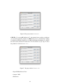
ProFiDo - The Processes Fitting
Toolkit Dortmund
Manual
Falko Bause, Souffian El-Baba, Philipp Gerloff, Alparslan Kirman, Jan Kriege,
Moussa Oumarou
Informatik IV, TU Dortmund
[email protected]
August 4, 2014
Contents
1
Introduction
2
Installation
2.1 License . . . . . . .
2.2 System Requirements
2.2.1 Linux . . . .
2.2.2 Windows . .
2.3 Installing ProFiDo .
2.3.1 Linux . . . .
2.3.2 Windows . .
3
.
.
.
.
.
.
.
3
3
3
4
4
4
4
4
3
Quick Start Guide
3.1 Specification of an Example Workflow . . . . . . . . . . . . . . . . .
3.2 Executing the Workflow . . . . . . . . . . . . . . . . . . . . . . . .
6
6
12
4
Working with ProFiDo
4.1 Commandline Parameters . . . . . . .
4.2 Workflow Specification and Execution
4.2.1 General Outline . . . . . . . .
4.2.2 Building a Workflow . . . . .
4.2.3 Executing a Workflow . . . .
4.3 ProFiDo’s Menu Structure . . . . . .
4.3.1 The File Menu . . . . . . . .
4.3.2 The Workflow Menu . . . . .
4.3.3 The Edit Menu . . . . . . . .
4.3.4 The Settings Menu . . . . . .
4.3.5 The Help Menu . . . . . . . .
4.3.6 Context Menus . . . . . . . .
4.4 Supported Tools . . . . . . . . . . . .
4.4.1 Distribution Fitting . . . . . .
4.4.2 Fitting of Stochastic Processes
4.4.3 Trace Generation . . . . . . .
4.4.4 Statistical Two Sample Tests .
4.4.5 Result Visualisation . . . . .
.
.
.
.
.
.
.
.
.
.
.
.
.
.
.
.
.
.
.
.
.
.
.
.
.
.
.
.
.
.
.
.
.
.
.
.
.
.
.
.
.
.
.
.
.
.
.
.
.
.
.
.
.
.
.
.
.
.
.
.
.
.
.
.
.
.
.
.
.
.
.
.
.
.
.
.
.
.
.
.
.
.
.
.
.
.
.
.
.
.
.
.
.
.
.
.
.
.
.
.
.
.
.
.
.
.
.
.
.
.
.
.
.
.
.
.
.
.
.
.
.
.
.
.
.
.
.
.
.
.
.
.
.
.
.
.
.
.
.
.
.
.
.
.
.
.
.
.
.
.
.
.
.
.
.
.
.
.
.
.
.
.
.
.
.
.
.
.
.
.
.
.
.
.
.
.
.
.
.
.
.
.
.
.
.
.
.
.
.
.
.
.
.
.
.
.
.
.
.
.
.
.
.
.
.
.
.
.
.
.
.
.
.
.
.
.
.
.
.
.
.
.
.
.
.
.
.
.
.
.
.
.
.
.
.
.
.
.
.
.
.
.
.
.
.
.
.
.
.
.
.
.
.
.
.
.
.
.
.
.
.
.
.
.
.
.
.
.
.
.
.
.
.
.
.
.
.
.
.
.
.
.
.
.
.
.
.
.
.
.
.
.
.
.
.
.
.
.
.
.
.
17
17
18
18
18
21
23
23
24
25
25
26
26
27
27
31
37
37
38
A Developing ProFiDo
A.1 Integrating additional tools . . . . . . . . . . . . . . . . .
A.1.1 Job Nodes . . . . . . . . . . . . . . . . . . . . . .
A.1.2 Input and Output Nodes . . . . . . . . . . . . . .
A.2 Test Manager . . . . . . . . . . . . . . . . . . . . . . . .
A.2.1 TestManager class . . . . . . . . . . . . . . . . .
A.2.2 Bash scripts perform_tests.sh and perform_diffs.sh
.
.
.
.
.
.
.
.
.
.
.
.
.
.
.
.
.
.
.
.
.
.
.
.
.
.
.
.
.
.
.
.
.
.
.
.
41
41
41
41
42
42
43
.
.
.
.
.
.
.
.
.
.
.
.
.
.
.
.
.
.
.
.
.
.
.
.
.
.
.
.
.
.
.
.
.
.
.
.
.
.
.
.
.
.
.
.
.
.
.
.
.
.
.
.
.
.
.
.
.
.
.
.
.
.
.
.
.
.
.
.
.
.
.
.
.
.
.
.
.
.
.
.
.
.
.
.
.
.
.
.
.
.
.
.
.
.
.
.
.
.
.
.
.
.
.
.
.
.
.
.
.
.
.
.
.
.
.
.
.
.
.
.
.
.
.
.
.
.
.
.
.
.
.
.
.
.
.
.
.
.
.
.
.
.
.
.
.
.
.
.
.
.
.
.
.
.
.
.
.
.
.
.
.
.
.
.
.
.
.
.
.
.
.
.
.
.
.
.
.
.
.
.
References
45
Index
47
1
List of Figures
1
2
3
4
5
6
7
8
9
10
11
12
13
14
15
16
17
18
19
20
21
22
23
24
25
26
27
28
29
30
31
32
33
34
35
36
37
38
39
40
41
Empty Workflow . . . . . . . . . . . . . . . . . .
Adding an input file node . . . . . . . . . . . . .
Selecting the input filename . . . . . . . . . . . . .
Positioning the input node . . . . . . . . . . . . .
Inserting a job node . . . . . . . . . . . . . . . . .
Example of a parameter window of a job node . . .
Canvas with several job nodes . . . . . . . . . . .
Adding an output file . . . . . . . . . . . . . . . .
Selecting the type of output . . . . . . . . . . . . .
Positioning the output node . . . . . . . . . . . .
Connecting with destination node . . . . . . . . .
Result after connecting two nodes . . . . . . . . .
Example of a complete workflow . . . . . . . . . .
Plot of autocorrelations for the workflow of Fig. 13
Plotter functionality . . . . . . . . . . . . . . . . .
Property window of the Edge View Plot . . . . . .
Property window of the Edge View Print . . . . . .
Complete workflow after positioning points . . . .
Plotter functionality . . . . . . . . . . . . . . . . .
Property window of the Edge View Plot . . . . . .
Property window of the Edge View Print . . . . . .
File Menu . . . . . . . . . . . . . . . . . . . . . .
Workflow Menu . . . . . . . . . . . . . . . . . . .
Edit Menu . . . . . . . . . . . . . . . . . . . . . .
Settings Menu . . . . . . . . . . . . . . . . . . . .
Help Menu . . . . . . . . . . . . . . . . . . . . .
Property window of DistFit . . . . . . . . . . .
Property window of G-FIT . . . . . . . . . . . .
Property window of Momfit . . . . . . . . . . . .
Property window of MAP_EM . . . . . . . . . . . .
Property window of MAP_MOEA . . . . . . . . . .
Property window of JMomfit . . . . . . . . . . .
Property window of ACfit . . . . . . . . . . . .
Property window of MEPfit . . . . . . . . . . . .
Property window of ARIMA Fitting . . . . . .
Property window of ARTAfit . . . . . . . . . . .
Property window of CAPP-Fit . . . . . . . . . .
Property window of Modgen . . . . . . . . . . . .
Property window of Plot . . . . . . . . . . . . .
Property window of Print . . . . . . . . . . . .
Property window of Queue . . . . . . . . . . . .
2
.
.
.
.
.
.
.
.
.
.
.
.
.
.
.
.
.
.
.
.
.
.
.
.
.
.
.
.
.
.
.
.
.
.
.
.
.
.
.
.
.
.
.
.
.
.
.
.
.
.
.
.
.
.
.
.
.
.
.
.
.
.
.
.
.
.
.
.
.
.
.
.
.
.
.
.
.
.
.
.
.
.
.
.
.
.
.
.
.
.
.
.
.
.
.
.
.
.
.
.
.
.
.
.
.
.
.
.
.
.
.
.
.
.
.
.
.
.
.
.
.
.
.
.
.
.
.
.
.
.
.
.
.
.
.
.
.
.
.
.
.
.
.
.
.
.
.
.
.
.
.
.
.
.
.
.
.
.
.
.
.
.
.
.
.
.
.
.
.
.
.
.
.
.
.
.
.
.
.
.
.
.
.
.
.
.
.
.
.
.
.
.
.
.
.
.
.
.
.
.
.
.
.
.
.
.
.
.
.
.
.
.
.
.
.
.
.
.
.
.
.
.
.
.
.
.
.
.
.
.
.
.
.
.
.
.
.
.
.
.
.
.
.
.
.
.
.
.
.
.
.
.
.
.
.
.
.
.
.
.
.
.
.
.
.
.
.
.
.
.
.
.
.
.
.
.
.
.
.
.
.
.
.
.
.
.
.
.
.
.
.
.
.
.
.
.
.
.
.
.
.
.
.
.
.
.
.
.
.
.
.
.
.
.
.
.
.
.
.
.
.
.
.
.
.
.
.
.
.
.
.
.
.
.
.
.
.
.
.
.
.
.
.
.
.
.
.
.
.
.
.
.
.
.
.
.
.
.
.
.
.
.
.
.
.
.
.
.
.
.
.
.
.
.
.
.
.
.
.
.
.
.
.
.
.
.
.
.
.
.
.
.
.
.
.
.
.
.
.
.
.
.
.
.
.
.
.
.
.
.
6
7
7
8
9
9
10
10
11
11
12
13
14
15
16
16
17
20
21
21
22
23
24
25
25
26
28
29
30
31
32
33
34
34
35
36
36
37
38
39
40
1
Introduction
ProFiDo (Processes Fitting Toolkit Dortmund) is a flexible environment written in Java
for realising different steps of input modeling. ProFiDo offers a GUI to combine various command line tools realising steps of data preprocessing, parameter fitting and
analysing the resulting processes into a workflow. In the current version (effective
August 2014), ProFiDo supports fitting of common distributions, Phase-type (PH) distributions, Markovian Arrival Processes (MAPs), Correlated Acyclic Phase-Type Processes (CAPPs), AutoRegressive To Anything (ARTA) processes and AutoRegressive
Integrated Moving Average (ARIMA) models from trace data and the analysis of these
distributions and processes. The theoretical background on these stochastic processes
is out of scope of this manual. Readers not familiar with these processes are referred
to [16, 17] for PH distributions and MAPs, to [15] for CAPP processes, to [10] for
ARTA processes and to [7] for ARIMA models.
For a general overview of ProFiDo’s key features and the motivation that led to the
development of ProFiDo the reader is referred to [1, 4]. Technical documentation on
the different file formats that ProFiDo uses for its configuration, for saving workflows
and for the description of stochastic processes can be found in [2, 3, 6].
This document is structured as follows. Installation instructions for ProFiDo are
given in Sect. 2. Sect. 3 contains an introductory tutorial and Sect. 4 explains the use
of ProFiDo in detail.
2
Installation
The latest version of ProFiDo can be obtained as a zip archive from
http://ls4-www.cs.tu-dortmund.de/profido
The archive contains the GUI ProFiDo and a collection of tools for fitting stochastic processes and result visualisation. The GUI is released under the GPL (see Sect. 2.1)
and the sources are available on the website as well. The included tools are currently
only available as binaries.
2.1
License
ProFiDo is free software, released under the terms of the GNU General Public License version 2 as published by the Free Software Foundation. ProFiDo is distributed
in the hope that it will be useful, but WITHOUT ANY WARRANTY; without even
the implied warranty of MERCHANTABILITY or FITNESS FOR A PARTICULAR
PURPOSE. See the GNU General Public License for more details.
2.2
System Requirements
ProFiDo is available for Linux and Windows. Depending on the operating system
different requirements have to be fulfilled to run ProFiDo.
3
2.2.1
Linux
To run ProFiDo’s GUI only Java is required. However, for full functionality including
all the supported tools for fitting and result visualisation the following system requirements have to be fulfilled:
• Linux
• Java
• wish - Tcl/Tk shell required for converter scripts
• gnuplot - required for creating plots of autocorrelation, cdf and pdf
• R - required for ARIMA fitting and statistical tests [23]
2.2.2
Windows
The Windows version of ProFiDo is bundled with a MSYS1 environment that contains
most of the tools required by ProFiDo. For the Windows version only Java is needed.
2.3
Installing ProFiDo
2.3.1
Linux
1. Extract profido1.3.zip to a local directory (the recommended directory is
~/ProFiDo):
mkdir ~/ProFiDo
unzip profido1.3.zip -d ~/ProFiDo
The directory should now contain four files (profido.jar, software.xml,
profido.sh, gpl-2.0.txt) and a subdirectory (software).
2. If you did not use ~/ProFiDo as installation directory you have to edit the file
software.xml and replace ${HOME}/ProFiDo in line
<softwaresource>${HOME}/ProFiDo/software</softwaresource>
at the beginning of the file with your installation directory.
3. Change to your installation directory and run ./profido.sh to start ProFiDo’s
GUI.
2.3.2
Windows
1. Right click profido1.3_win.zip and select "Extract..." from the files context menu and choose a target folder (the recommended directory is C:\). Note
that the identifier of the selected target folder must not contain a blank or other
white space characters!
1
http://www.mingw.org/wiki/msys/
4
Afterwards the selected directory will hold a subfolder called MinGW which
contains the preconfigured MinGW/MSYS environment and the entire ProFiDo
software.
2. Open the subfolder MinGW/msys/1.0 within the target directory and execute
msys.bat to start a MSYS shell. Within this MSYS shell type cd profido
to change to the ProFiDo directory and run ./profido.sh to start ProFiDo’s
GUI.
5
3
Quick Start Guide
The following sections explain step-by-step how ProFiDo’s GUI can be used to build
up an example workflow description and how this workflow can be executed. This
quick-start guide will only explain the basic functionality that is necessary to specify
the example workflow and gives a first overview of the features of ProFiDo. A detailed
description of ProFiDo that introduces all the features and properties will be given in
Sect. 4.
3.1
Specification of an Example Workflow
In the following we will assume that the user wants to create a simple workflow to
fit MAPs to a given trace file using two different fitting approaches. To assess the
quality of the fitted MAPs some characteristics of the MAPs and the trace file should
be visualised.
1. Starting ProFiDo by calling profido.sh gives a window with an empty canvas as shown in Fig. 1.
Figure 1: Empty Workflow
2. Describing a workflow means essentially to describe a graph with edges and
nodes. So let us start with the first node of the graph describing an input file.
Input files are usually trace files that contain observations from a real system
and that we want to fit with a stochastic process. For selecting an input file click
on Workflow in the menu bar and select Add Input File (see Fig. 2).
This will open a dialog window, where one can select the input file (see Fig. 3).
After that the node which is associated with the input file is placed with a click
into the canvas window (see Fig. 4). For our example workflow we opened the
trace LBL-TCP-3 [22] from the Internet Traffic Archive [25] that was reduced
to contain only the interarrival times. This version of the trace is also available
from ProFiDo’s website (see Sect. 2).
6
Figure 2: Adding an input file node
Figure 3: Selecting the input filename
7
Figure 4: Positioning the input node
3. In a similar manner other nodes can be placed on the canvas. E.g. to insert the
call of a fitting tool into the workflow click on Workflow in the menu bar and
select the specific type of job using Add Job (see Fig. 5). After positioning the
node a window will pop up where job specific parameters can be specified (see
Fig. 6).
For the example workflow two MAP fitting algorithms are added to the workflow, in particular a tool called ACfit that fits a MAP according to the lag-k
autocorrelations of the trace and a tool called JMomfit that uses the empirical
joint moments for fitting. Since both tools expect a PH distribution as input, we
place the tool Momfit that fits a PH distribution according to the moments of a
trace on the canvas.
Since we want to assess the quality of the fitting algorithms we add the tools
Plot and Print to the workflow. Plot can create figures showing different properties of the models like autocorrelations or the distribution function.
Print has a similar function for statistical properties that should be output in
textual format and can for example generate a LATEX table.
Fig. 7 shows the canvas with all tools added so far. Note, that the tool specific
parameters that are entered in the property window from Fig. 6 are displayed
above the different job nodes. Thus, Momfit will use the first 9 empirical
moments from the trace to fit a PH distribution with 3 states and run for 20000
iterations. JMomfit will consider the first 5 × 5 joint moments and ACfit
the first 10 lags of autocorrelation. Plot will create a PostScript (PS) image
plotting the first 10 lags of autocorrelation and Print will create a LATEX table
with the first 5 joint moments. A detailed description of the different tools and
their parameters will be given in Sect. 4.
4. To define the outputs of the workflow, one can specify output nodes. Defining
an output file is similar to specifying an input file. Select Add Output File
8
Figure 5: Inserting a job node
Figure 6: Example of a parameter window of a job node
9
Figure 7: Canvas with several job nodes
in the menu bar (see Fig. 8) and choose the directory where the output file shall
be stored and specify its name. Afterwards a window pops up where you can
select the type of output (see Fig. 9). Finally the node representing the output
file is positioned on the canvas (see Fig. 10). For our example we place two
output nodes on the canvas, one for a PostScript file (lbl_ac.ps) and one for
a LATEX file (lbl_jmom.tex).
Figure 8: Adding an output file
5. To complete the workflow description nodes have to be connected by edges.
In order to connect two nodes by a direct arc first click on the source node
10
Figure 9: Selecting the type of output
Figure 10: Positioning the output node
11
such that the node is highlighted. Afterwards right-click on the destination node
and select the first option Connect output from selected node to
this (see Fig. 11) which results in a directed arc connecting source and destination node (see Fig. 12).
In a similar way all other arcs can be created completing the workflow specification (see Fig. 13).
Of course, arcs may be created at any time during the workflow specification,
not only after all the nodes have been placed.
Each arc contains a label with the model type for the model description that is
propagated between the two nodes. Additionally, a file name is associated with
each connection. ProFiDo will automatically determine an unique file name for
each arc such that no conflicts occur. However, in some cases it is desirable to
manually chose a file name. For example the tools Plot and Print use the
file names as labels for the curves of the plot or for the columns of the table.
Observe from Fig. 13 that we changed the file names at the arcs from JMomfit
and ACfit to Plot and Print to MAP3_JM.xml and MAP3_AC.xml. The
file name can be changed by selecting Edit Connection from the context
menu of the arc.
Figure 11: Connecting with destination node
3.2
Executing the Workflow
Once the workflow specification is complete, the entire workflow can be exported to
a shell script and be executed. Select Export Workflow as Script from the
Workflow menu and choose a file name to export the workflow. ProFiDo will create
two shell scripts (<name>_setup.sh and <name>.sh) that setup all the necessary
tools and execute the tools of the workflow. ProFiDo automatically sorts the order of
execution of the different tools corresponding to the job nodes according to their order
12
Figure 12: Result after connecting two nodes
in the workflow. Call <name>_setup.sh to setup the tools for the workflow. After
that the workflow can be executed by calling <name>.sh.
In addition to the export of the normal workflow an extended workflow with additional report can be created. Select Export Workflow as Script with
Report and choose a file name accordingly. ProFiDo will export the above described
workflow scripts and two additional files (<name>_report.sh and <name>_report.tex)
located in directory Results/Report. The <name>_report.sh script will be
called after the execution of the workflow and creates a versatile PDF report file containing all properties of the workflow and its intermediate as well as final results.
The PDF report file is generated from LATEX files generated by ProFiDo, which can
be used as a basis for further documentation. The LATEX files are located in directory
Results/Report/Files.
Table 1: Joint moments for the workflow from Fig. 13
Joint Moment
1, 1
2, 2
3, 3
4, 4
5, 5
lbl3_dat
1.30
17.42
890.5
107474
21417760
MAP3_JM
1.29
17.65
890.5
105484
22268852
MAP3_AC
1.30
15.97
673.9
70378
14002609
The execution of the example workflow will result in two files as specified by the
13
Figure 13: Example of a complete workflow
14
Autocorrelations for lags 1-10
0.16
lbl3_dat
MAP3_AC
MAP3_JM
0.14
autocorrelation
0.12
0.1
0.08
0.06
0.04
0.02
0
1
2
3
4
5
6
7
8
9
10
lag
Figure 14: Plot of autocorrelations for the workflow of Fig. 13
output nodes in Fig. 13. The plot with the autocorrelations is shown in Fig. 14. Table 1
shows the joint moments created by the Print node. Observe, that the curves in
Fig. 14 and the columns in Table 1 are labeled with MAP3_AC and MAP3_JM which
corresponds to the file names we entered at the incoming arcs of Plot and Print in
Fig. 13.
Once the workflow has been executed, the Edge View functionality can be used
to display intermediate results. In order to do this right-click on the edge and select
the option Plot Details (see Fig. 15). The menu item Plot Details opens a
window similar to the parameters window of the job node Plot (see Fig. 16). After
confirming the values with a click on the OK button the characteristics of the selected
model are displayed in a new window. In addition to the graphical view a text based
display of intermediate results is also possible. To display textual informations select
the option Print Details (see Figs. 15 and 17).
15
Figure 15: Plotter functionality
Figure 16: Property window of the Edge View Plot
16
Figure 17: Property window of the Edge View Print
4
Working with ProFiDo
In the following we will explain in detail how ProFiDo can be used for fitting stochastic
processes. In Sect. 4.2 the workflow specification and execution is presented. Sect. 4.3
gives a detailed overview on ProFiDo’s menu structure and the functions available
from the menu bars. Finally, in Sect. 4.4 we give some background on the tools that
are currently integrated into ProFiDo and introduce their parameters.
4.1
Commandline Parameters
ProFiDo can be called with various commandline parameters to load an existing workflow or to perform automated tests. Most of the commandline parameters are used to
control the integrated Test Manager which is explained in Appendix A in detail. If no
parameters are given ProFiDo will start with an empty canvas.
ProFiDo can be called by
profido.sh [OPTIONS] [INPUT-FILE] [EXPORT-FILE]
where all parameters are optional. [INPUT-FILE] specifies a workflow to be loaded,
[EXPORT-FILE] a file name to store the workflow. [OPTIONS] may be any of the
following:
• -c <file>: Selects a custom configuration file. (Default: software.xml)
• -n: Disables all file existence checks when loading a workflow.
• -nv: Disables the XML validation.
• -h, --help: Displays usage information.
17
• -t <mode> <interactions>: Activates the TestManager in the selected
mode and performs the specified amount of user interactions. (Default: No mode
selected, interactions = 10)
• -d <delay>: Specifies a custom time in milliseconds between two user interactions within the TestManager. (Default: 5)
• -s <seed>: Specifies a custom seed for the TestManager. (Default: Time
since midnight, January 1, 1970 UTC in milliseconds.)
4.2
Workflow Specification and Execution
In ProFiDo the fitting of stochastic processes is described by workflows. Workflows
are composed of different nodes that represent different steps of data preprocessing,
fitting and result visualisation. Each node of the workflow corresponds to a tool that
is responsible for performing one of these steps. The nodes are connected by arcs
to determine the order of execution of the tools and the result propagation from one
tool to the next. In this way it is possible to specify complex workflows consisting of
various connected tools in a graphical manner.
4.2.1
General Outline
A workflow is represented by a graph composed of a minimum of the following nodes:
• At least one input node associated with an input file, which usually is a trace file
or a stochastic process in ProFiDo’s XML interchange format [6].
The first entry of a trace file is the number of subsequent elements in that file.
All other entries are interpreted as data values, e.g. inter-arrival times, packet
sizes etc.
• One or several job nodes each representing a particular tool. Detailed descriptions of the tools will be given in Sect. 4.4.
• One or several output nodes associated with an output file. Possible outputs
are traces, stochastic processes in different formats (like ProFiDo’s XML interchange format or Nsolve’s [18] format for MAP descriptions) and image or
LATEX files for various plots and tables with characteristics of stochastic processes and traces.
An example of a workflow is shown in Fig. 13.
4.2.2
Building a Workflow
Specification of a workflow can be done by placing nodes on the grid and connecting
them with directed arcs. The connection has to observe certain rules.
18
Placing nodes on the grid ProFiDo distinguishes three types of nodes: Input nodes,
job nodes and output nodes.
• Input nodes are the first nodes of a workflow and have no predecessor. Input
nodes are used to specify files that are used as input for the workflow. In most
cases the input nodes will be used to load a trace file.
To add an input node, select Add Input File from the Workflow menu.
Afterwards a file selection window will pop up where you can select the input
file. In the next dialog window the type of the file has to be chosen. After
that, one can place the input node on the grid by clicking on the corresponding
position in the canvas.
• Job nodes are the basic building blocks of a workflow that perform the actual fitting tasks. Each job node corresponds to one of the tools presented in Sect. 4.4.
To place a job node on the grid, select one of the tools from Workflow ->
Add Job. After positioning the job node by clicking on the grid a window
with tool specific parameters is shown. Each job is defined by a set of parameters and the number of parameters might vary dependent on the job type. The
meaning of the parameters is also explained in Sect. 4.4. The user can edit parameters by changing the default values. Each parameter has two check boxes,
where the user can select whether the parameter will be enabled and/or be visible on the grid. Only enabled parameters will later be relevant when calling
the corresponding tool. A summary with all parameters whose visibility flag is
set to true is displayed above the job node on the canvas. Additionally, all parameters are displayed in a tooltip when the mouse pointer is over the job node.
Furthermore an optional description of a parameter is displayed when the user
clicks on the associated question mark ? (cf. Fig. 28).
• Output nodes are the counterpart of input nodes and mark the end of a workflow. Thus, defining output nodes is similar to the definition of input nodes.
Select Workflow -> Add Output File and specify name and location
within the shown file selection window. Afterwards you will be asked to select
the output type of the file. After that the output node can be placed on the grid.
Output nodes are used to specify the results of a workflow that the user is interested in. For example they might be used to save the fitted models or some plots
with characteristics of the models.
Connecting nodes To complete a workflow description the nodes of the workflow
have to be connected by directed arcs. These arcs determine the order of execution
of the different jobs and the propagation of intermediate results, e.g. if two nodes are
connected, the output of the first node will be used as input for the second node.
The connection of two nodes by a directed arc is done as follows. First select the
source node, then right click on the target node. A pop-up menu will appear which
allows different operations. Select Connect output from selected node
to this to connect the two nodes. Note, that two nodes can only be connected,
if the output of the first node is an allowed input for the second node. In particular,
input nodes have no predecessor and output nodes no successor. Input nodes may be
connected with job nodes, if the job node can process the input file and job nodes
19
may always be connected with an output node. Connections between job nodes are
allowed, if the output of the first job matches an expected input of the second job.
Sect. 4.4 contains all the expected inputs and outputs of job nodes.
Usually, an arc is a straight line from one node to another. In some cases this might
not result in the best layout for the workflow, e.g. if the arc crosses other arcs or
nodes. Therefore, each arc comprises one or more (green) points which can be freely
positioned on the canvas to give a more readable graph layout (see Fig. 18). Additional
points may be added by right-clicking on one of the existing points. By default, all
points are automatically positioned by ProFiDo. To position points freely on the canvas
the option Auto Position has to be disabled.
The parameters of a connection are the file type and file name associated with the
output of a node and the order key. The file type is displayed if the option Display
Edge Information is enabled in the Settings Menu. All parameters are also
displayed as a tooltip if the cursor hovers over the corresponding point. The order key
can be used to establish the order of incoming arcs on a node. If a node can process
several incoming file parameters with the same type a lower order key is used first
when the shell script for workflow execution is built. Clicking on an existing point
allows for editing the three parameters of a connection between two nodes, which are
the file name and the file type that are used for storing the output of a node when
executing the workflow and the order key. By default ProFiDo determines file names
such that no conflicts will occur and the user does not have to care about the file names.
However, some job nodes (currently Plot and Print) use the file names as labels in
their output figures and tables. See Fig. 13 in Sect. 3 for an example.
Figure 18: Complete workflow after positioning points
An additional menu item (see Fig. 19) is offered to display characteristics of models (eg. CDF, ACF) directly. With the help of the Plot Details and Print
20
Details menu items it is possible to display intermediate results.
Figure 19: Plotter functionality
It should be noted that the script (cf. Sect. 4.2.3) must have been exported and
executed once before to use the Plot Details and Print Details functionality. A detailed description of the tools Plot and Print will be given in Sect. 4.4.
Clicking on the menu item Plot Details a window similar to the property window of the job node Plot will pop up (see Fig. 20). The behaviour of the item Print
Details is analogous (see Fig. 21).
With a click on the OK button the Plot / Print is executed with the edge file as
input and the characteristics of the selected model are displayed in a new window. To
ensure that everything works as described, the workflow must be saved after exporting.
Otherwise you will be prompted to specify the path of the exported script.
Figure 20: Property window of the Edge View Plot
4.2.3
Executing a Workflow
If the workflow description is complete, it can be exported to a bash script by selecting
Export Workflow as Script from the Workflow menu. Before the script is
21
Figure 21: Property window of the Edge View Print
generated ProFiDo checks the workflow for consistency. A correct workflow has to
fulfill the following conditions:
- A workflow has to be acyclic.
- A workflow must start with at least one input node and terminate with at least
one output node.
- Each input node must have at least one outgoing edge.
- Each output node mut have exactly one incoming edge.
- Each job node must have at least one incoming and one outgoing edge.
If these conditions are met a file dialog pops up where the user has to enter a filename. After entering a filename ProFiDo will generate two shell scripts: <name>.sh
and <name>_setup.sh . The execution of <name>_setup.sh will prepare the
workspace, i.e. setting up all the tools used in the workflow. After that <name>.sh
can be called to execute the actual workflow. <name>.sh contains all the calls to
the tools corresponding to the job nodes of the workflow. ProFiDo will automatically
determine the right order of the calls from the workflow layout. After the execution is
complete, the output files can be found in the location specified by the output nodes of
the workflow. Interim results can be found in directory Results. The file names in
this directory conform to the parameters of the node connections.
In addition to the normal export an extended workflow with additional report can
be created. After selecting Export Workflow as Script with Report ProFiDo
will export the above described workflow scripts and two additional files (<name>_report.sh
and <name>_report.tex). The <name>_report.sh script will be called after the execution of the Workflow and create a versatile PDF report file containing
22
all properties of the workflow and its intermediate as well as final results. All files
referenced and used by the report are in directory Results/Report. Note that report files <name>_report.sh and <name>_report.tex are directly generated
from ProFiDo’s GUI and are not generated by setup scripts.
Note, that the Results and the Report directories are not automatically deleted
by the generated scripts. It is in the user’s responsibility to save files that are still
needed from the folders and to delete them between the execution of different workflows to avoid confusion with old existing files.
4.3
ProFiDo’s Menu Structure
ProFiDo’s GUI offers five menu entries. These are
• File Menu,
• Workflow Menu,
• Edit Menu,
• Settings Menu and
• Help Menu
and will be described in the following. Additional functionality is available via various
context menus described at the end of this section.
4.3.1
The File Menu
The File Menu offers basic functionality for loading and saving workflows. The
menu is shown in Fig. 22.
Figure 22: File Menu
• New Workflow offers the possibility to create a new workflow.
• Load Workflow allows to load a workflow description from a file in XML
format as specified in [3].
• Save Workflow allows to save a workflow in a file using the XML Format
as specified in [3].
• Quit quits ProFiDo.
23
All File Menu options include a check for unsaved changes to the current workflow. A confirmation dialog will pop up remembering to save the current workflow, if
necessary.
4.3.2
The Workflow Menu
This menu contains all the ingredients for specifying a workflow (see Fig. 23). It offers
the following functions:
Figure 23: Workflow Menu
• Add Job offers the possibility to add a new job node into a workflow. For selection one of the available fitting tools supported by ProFiDo have to be chosen.
The tools currently supported by ProFiDo are presented in detail in Sect. 4.4.
• Add Output File. This item allows to insert an output node to the workflow.
• Add Input File. This item allows for the insertion of an input node.
• Change Workflow Name allows to change the name of the current workflow.
• Set Working Directory. The working folder/directory can be set by
clicking on this menu entry. The working folder is that folder/directory which
will be suggested by ProFiDo for storing output files or from where to import
input files.
• Export Workflow as Script. This item allows to export a bash script
which governs the execution of the specified workflow.
• Export Workflow as Script with Report. This item exports the
standard workflow script and all files needed to create the automatic report.
24
• Save Screenshot. This item allows to save a screenshot of the current
canvas content in Portable Network Graphics (PNG) format.
4.3.3
The Edit Menu
Figure 24: Edit Menu
The Edit Menu (cf. Fig. 24) offers basic undo/redo functionality, in particular:
• Undo the last performed action,
• Redo the last cancelled action,
• show all previously performed actions via the Show History item and
• delete the complete history.
Show History displays a list of all previously performed actions with the last
action being on bottom of the list. By selecting one of the previous actions one can
undo all later actions by selecting Move to selected state. It is also possible
to redo the changes by selecting a later action afterwards. The button Create Snapshot
saves the currently visible state of the workflow to an XML file in the ProFiDo directory.
4.3.4
The Settings Menu
This menu (cf. Fig. 25) allows for the definition of preferences, which influence the
GUI’s look and feel.
Figure 25: Settings Menu
• The Scale on resize checkbox determines whether the graph of the workflow will be resized when the window is resized or whether it will maintain its
original size.
25
• Display Grid determines whether a grid will be shown or not.
• Display Edge Information determines whether any information are displayed on the central point of the edge.
• Display Node Information determines whether the visible parameters
of a job node are displayed.
• Via the entries of the Debug menu one can override some of the above settings, i.e. some of the information on edges or nodes are always displayed if the
corresponding item from the menu is selected.
4.3.5
The Help Menu
The Help Menu (cf. Fig. 26) just gives more information about the tool.
Figure 26: Help Menu
4.3.6
Context Menus
Some of the functionality of nodes and edges is available via different context menus
that are selected by a right click on the node or on a green point of an edge.
Input Nodes and Output Nodes
• Connect output from selected node to this: This entry is used
to connect two nodes.
• Delete: Deletes the node
• Change External File Name: Selects another file for the node.
• Change External File Type: Changes the type of the file.
• Edit Comment: Edit the comment containing a description of this file.
Job Nodes
• Connect output from selected node to this: This entry is used
to connect two nodes.
• Delete: Deletes the node
26
• Edit: Opens the attribute window of the job node. The attributes displayed in
those windows depend on the type of job node (see Sect. 4.4 for all job nodes
and their corresponding attributes).
• Change Name: Changes the name of the job node that is displayed in the
canvas.
• Show Commandline Call: Prints the commandline call of the job node
that is used when exporting the workflow to a shell script.
• Edit Comment: Edit the comment containing a description of this job.
Edges
• Delete Connection: Deletes the connection.
• Edit Connection: Opens the attribute window of the edge, where the file
name, file type and order key can be changed (see Sect. 4.2 for an explanation
of these attributes). Additionally one can specify which of the attributes should
be displayed on the canvas.
• Add EdgePoint: Adds an additional point to the edge that can be used to
specify the pathway of the edge.
• Delete EdgePoint: Deletes the edge point provided it is not the sole point
of that edge.
• Auto Position: If enabled the selected edge point will be positioned automatically, otherwise it can be positioned manually within the grid.
• Plot Details: Opens the edge view plot window that can be used to plot
characteristics of the model that is propagated along the edge.
• Print Details: Opens the edge view print window that can be used to print
characteristics of the model that is propagated along the edge.
4.4
Supported Tools
ProFiDo currently supports several tools for fitting and analysing distributions and
stochastic processes that can be integrated into a workflow as job nodes (cf. Figs. 5
and 23). In the following these tools and their parameters will be introduced. Additionally, the generated output and the expected inputs are listed to clarify which of
the job nodes may be connected. We will only briefly introduce the basic ideas of the
different algorithms, but omit the full theoretical background. For the interested reader
some references providing this background information will be given.
4.4.1
Distribution Fitting
ProFiDo currently supports three tools for distribution fitting. DistFIT is a general tool
for fitting various common distributions whereas GFit and Momfit specialise on fitting
PH distributions.
27
DistFit DistFit provides parameter estimation for various common distributions
based on a given trace. For most distribution types the fitting is based on the MLE
(maximum likelihood estimator) [13] . A complete list of supported distributions, their
properties and the corresponding fitting approach can be found on the ProFiDo website
[5]. Fig. 27 shows the parameters of DistFit. Depending on the parameters entered
Figure 27: Property window of DistFit
the tool fits a single distribution or several distributions to the trace and determines the
one with the best likelihood value. The output of the tool is an XML file as specified
in the ProFiDo XML interchange format [6]. It contains the distribution with the
best likelihood value for the given trace as its first distribution tag. All other fitted
distributions (if any) are written as sub tags of a first level <info> tag sorted in order
of their likelihood value. Furthermore each <distribution> tag has an <info>
sub tag containing the likelihood value of the corresponding distribution for the given
trace. Note, that the information from the <info> tag is usually not used by other job
nodes.
• Input: Trace
• Output: Distribution
• Parameters:
– auto: Fit all supported distributions to the trace and select the one with
the best log-likelihood value.
– exponential: Fits an exponential distribution to the trace.
– normal: Fits a normal distribution to the trace.
– lognormal: Fits a lognormal distribution to the trace.
– johnson: Fits a Johnson distribution to the trace.
– uniform: Fits an uniform distribution to the trace.
– triangular: Fits a triangular distribution to the trace.
– erlang: Fits an Erlang distribution to the trace.
– gamma: Fits a gamma distribution to the trace.
28
G-FIT G-FIT [26] implements an EM Algorithm to fit the parameters of hyper
Erlang distributions maximising the likelihood value. Hyper Erlang distributions are a
subclass of PH distributions with a special structure resulting in an efficient algorithm
that can be applied to large traces. G-FIT can operate in two modes: Either a single
hyper Erlang distribution with a given structure is fitted or the best distribution with a
given overall number of states is determined. The parameters of G-FIT are shown in
Fig. 28. G-FIT can either use the complete trace for fitting or work on an aggregated
trace as described in [21].
Figure 28: Property window of G-FIT
• Input: Trace
• Output: PH distribution, MAP
• Parameters:
– Single Erlang: Fits a single hyper Erlang distribution to the trace.
The parameter is specified as a list of numbers, where the first number determines the number of Erlang branches and the following numbers define
the number of phases for each branch, e.g. 3 1 1 1 fits a hyper Erlang
distribution with 3 branches where each branch consists of 1 phase.
– All Erlang: Fits different settings of hyper Erlang distributions with
a given number of states and selects the distribution with the best likelihood value. The parameter is specified as a list of 3 values, where the first
value determines the overall number of states, the second value the minimal number of Erlang branches and the third value the maximal number
of branches. Note, that only one of the parameters Single Erlang or
All Erlang may be enabled.
29
– Conv. e: Determines the value for the convergence check. If the
values between two iterations of the EM algorithm improve less than the
optimisation stops.
– Conv. Check: Determines the type of convergence check. If checked,
the maximal difference between parameter values of the distribution is
used, otherwise the difference between log-likelihood values.
– Logarithmic Trace aggregation: If enabled this value specifies
the number of intervals that are used to aggregate the trace on a logarithmic
scale.
– Uniform Trace aggregation: If enabled this value specifies the
number of intervals that are used to aggregate the trace.
Momfit Momfit [9] fits the parameters of an acyclic PH distribution by applying a
non linear optimisation algorithm according to the moments of the trace. The optimisation approach minimises the least squares difference between the weighted moments
of the trace and the fitted distribution and is independent of the length of the trace.
Fig. 29 shows the property window of Momfit.
Figure 29: Property window of Momfit
• Input: Trace
• Output: PH distribution, MAP
• Parameters:
– Moments: The number of empirical moments of the trace that should be
considered for fitting.
30
– States: The order (i.e. the number of transient states) of the PH distribution.
– The algorithms stops, if either the number of Iterations has been
reached, the difference between the results of two subsequent iterations
is smaller than Epsilon or Time has been reached.
– Seed: Seed of the random number generator that is used to determine the
initial random PH distribution.
4.4.2
Fitting of Stochastic Processes
ProFiDo currently supports two types of stochastic processes, namely MAPs and ARIMA/ARTA/CAPP models, and a variety of different fitting algorithms for these processes:
MAP_EM MAP_EM [8] applies an EM approach to the whole trace. The approach
is time consuming so that it should not be applied to fit MAPs with a larger state
space to long traces. However, since EM algorithms have a monotonic convergence,
the algorithm can be used to improve the likelihood of a MAP that has been fitted by
some other more efficient approach. In case only a trace file is provided as input the
algorithm will start with a random MAP, if additionally an existing MAP is provided
as input, the algorithm will use this MAP as initial solution and improve its likelihood.
The tool specific properties are shown in Fig. 30.
Figure 30: Property window of MAP_EM
• Input: Trace, MAP (optional)
• Output: MAP
• Parameters:
31
– Conv. e and #Iteration are used to specify the stopping criterion
for the algorithm. If either the improvement of the algorithm is less than
or the specified number of iterations have been reached, the algorithm
stops.
– MAP Dims determines the order of the MAP, i.e. the number of states.
– Alpha is a factor used for the randomisation technique.
– Seed of the random number generator used to generate the random initial
MAP.
MAP_MOEA MAP_MOEA [20] combines an EM algorithm for PH distribution fitting with a multi-objective evolutionary algorithm to fit a MAP. Its parameters are
shown in Fig. 31.
Figure 31: Property window of MAP_MOEA
• Input: Trace
• Output: MAP
• Parameters:
– Number of Generation determines how many generations the evolutionary algorithm should use.
32
– Alpha, Mu and Lambda are parameters for the evolutionary algorithm.
They determine the population size α, the number of parent individuals µ
and the number of offspring individuals λ.
– Epsilon: Stopping criterion for the EM part of the algorithm. If the
improvement of the algorithm is less than the EM algorithm will stop.
– #Iteration determines the number of iterations of the EM algorithm
in the first fitting step.
– Dimension determines the order of the MAP, i.e. the number of states.
– Alpha2 is a factor used for the randomisation technique.
– Seed of the random number generator used to generate the random initial
MAP.
– Autocorrelation determines the number of lag-k autocorrelations
that are used for MAP fitting.
JMomfit JMomfit [9] performs a least squares fitting of the weighted joint moments of the trace and the fitted MAP. It is started with a PH distribution that is expanded into a MAP. Consequently, the node expects a trace and a PH distribution as
input. Since only linear least squares problems have to be solved and joint moments
are fitted, the approach is very efficient and the effort is independent of the length of
the trace. The parameter window is shown in Fig. 32.
Figure 32: Property window of JMomfit
• Input: Trace, PH distribution
• Output: MAP
• Parameters:
– Joint Moments: The number n of joint moments to be considered for
fitting. The algorithm will use the first n × n joint moments from the trace.
ACfit ACfit [14] takes a trace and a PH distribution as input and fits a MAP according to the lag-k autocorrelations of the trace. This implies the use of a non linear
optimisation method so that the effort becomes slightly higher than that for joint moment fitting, but the effort is still independent of the trace length. Fig. 33 shows the
parameters of ACfit.
33
Figure 33: Property window of ACfit
• Input: Trace, PH distribution
• Output: MAP
• Parameters:
– Autocorrelation: The number of empirical autocorrelations from the
trace that should be considered for fitting.
MEPfit From a set of moments and joint moments the algorithm constructs two
matrices H0 and H1 as described in [24, 27] and tries to transform them into a valid
MAP description (D0 , D1 ) by searching for a non-singular matrix B such that D0 =
B−1 H0 B and D1 = B−1 H1 B. It should be noted, that the last step might fail, if
there is no MAP that exhibits the desired (joint) moments or if the method does not
find such a MAP. In this case the best matrices that have been found are returned,
which either describe a Matrix Exponential Process (MEP) or may not even describe a
stochastic process at all. Fig. 34 shows the parameters of MEPfit.
Figure 34: Property window of MEPfit
• Input: Trace
• Output: MAP
• Parameters:
– Order: The number of states of the MAP.
34
ARIMA Fitting The free software R [23] contains a large number of statistical methods including methods to determine the parameters of ARIMA models, that are used in
ProFiDo to generate ARIMA processes from trace data. Fig. 35 shows the parameters
of the node ARIMA Fitting.
Figure 35: Property window of ARIMA Fitting
• Input: Trace
• Output: ARIMA process
• Parameters:
– AR Order, Degree of Differencing and MA Order specify the
order of the ARIMA process, i.e. the number of autoregressive coefficients
p, the degree of differencing d and the number of moving average coefficients q.
ARTAfit For a given distribution FY and empirical autocorrelation coefficients of a
trace this approach constructs an ARMA base process, such that the resulting ARTA
process with marginal distribution FY exhibits the desired autocorrelations from the
trace. For more details see [11]. Fig. 36 shows the parameters of the node ARTAfit.
• Input: Distribution, Trace
• Output: ARTA process
• Parameters:
– Autocorrelations: Determines the number of autocorrelation coefficients that are considered for fitting.
– min. AR order, max. AR order, min. MA order, max.
MA order: Determines the order of the base process. ARTAfit will
fit base processes for all possible combinations given by the minimal and
maximal AR and MA order and select the base process with the best result.
35
Figure 36: Property window of ARTAfit
CAPP-Fit For a given PH distribution FY and empirical autocorrelation coefficients
of a trace this approach constructs an ARMA base process, such that the resulting
Correlated Acyclic Phase-Type Process (CAPP) with marginal distribution FY exhibits
the desired autocorrelations from the trace. For more details see [15]. Fig. 37 shows
the parameters of the node CAPP-Fit.
Figure 37: Property window of CAPP-Fit
• Input: PH Distribution, Trace
• Output: CAPP
• Parameters:
36
– Autocorrelations: Determines the number of autocorrelation coefficients that are considered for fitting.
– min. AR order, max. AR order, min. MA order, max.
MA order: Determines the order of the base process. CAPP-Fit will
fit base processes for all possible combinations given by the minimal and
maximal AR and MA order and select the base process with the best result.
4.4.3
Trace Generation
Modgen This job node allows for the generation of a trace from a given model description. Only a single model description is allowed as input. The trace length can
be defined by setting parameter TraceLength. Fig. 38 shows the parameters of the
node Modgen.
Figure 38: Property window of Modgen
• Input: Distribution, PH distribution, MAP, CAPP, ARIMA or ARTA process
• Output: Trace
• Parameters:
– TraceLength determines the length of the generated trace.
4.4.4
Statistical Two Sample Tests
Dist_Tests Job node Dist_Tests applies statistical two sample tests offered by
the statistical software R [23] in this way validating the hypothesis that two samples
are from the same distribution. The result is a LATEX table giving the P-values of the
applied tests. At present, Kolmogorov-Smirnov and Pearson’s Chi-Squared tests are
supported.
Job node Dist_Tests needs no parameters specified by the user and exactly two
inputs, i.e. two input arcs, of type XML-Trace are needed for proper functioning.
• Input: Two Traces
• Output: Table in LATEX format
• Parameters: NONE
37
4.4.5
Result Visualisation
Plot The Plot node helps to visualise model characteristics such as cumulative distribution functions and autocorrelation lags for given model descriptions or traces. Its
properties are shown in Fig. 39.
Figure 39: Property window of Plot
• Input: any number of Traces, distributions, PH distributions, MAPs, CAPPs,
ARIMA and ARTA processes
• Output: Image in PostScript, PDF or PNG format
• Parameters:
– Format: File format of the generated output image. Allowed values are
ps for PostScript, pdf for Portable Document Format or png for Portable
Network Graphics.
– Start and End determine the range on the x-axis that is plotted (cf. Fig. 14).
– Type: Type of plot. Possible values are ac for lag-k autocorrelation coefficients, cdf for the cumulative distribution function, pdf for the probability density function, mom for moments and jmom for joint moments.
For mom the moments E[X i ] for all i in the range from Start to End
are determined for all models and the values relative to the moments of the
first model are plotted. For jmom the joint moments E[X0i X1i ] are used.
Print The Print node offers the possibility to generate LATEX tables containing
several characteristic figures of process descriptions. Currently supported are moments
and joint moments. Fig. 40 shows the tool specific properties.
• Input: any number of Traces, distributions, PH distributions, MAPs, CAPPs,
ARIMA and ARTA processes
• Output: Table in LATEX format (cf. Table 1)
38
Figure 40: Property window of Print
• Parameters:
– Format: File format of the generated output. Currently only latex is
supported.
– Relative: If true the (joint) moments are computed relative to the values
of the first model (i.e. the model resulting from the job node that has been
connected first to the Print node). If false the absolute values are
printed.
– Start and End determine the first and last value to be computed.
– Type: Type of data to be printed. Possible values are ac for lag-k autocorrelation coefficients, cdf for the cumulative distribution function, pdf
for the probability density function, mom for moments and jmom for joint
moments.
Queue The Queue node is an additional way to compare processes. This job node
simulates a single server queue with a trace or stochastic process as input and returns
a plot of the queue length distribution.2 The unit of measurement for the interarrival
times used as input for the queue are in seconds. Fig. 41 shows the tool specific properties. The Queue node expects the service time, the buffer size and the simulation
time as additional parameters. The job node uses OMNeT++ [12] as simulation engine
and therefore the service time must be specified in OMNeT++’s syntax (see below).
• Input: any number of Traces, MAPs, CAPPs, ARTA and ARIMA processes
• Output: Image in PostScript
2
The value given for queue length i is the sum of all time intervals where i customers have been in
the queue divided by the overall simulation time. Note that the given queue length distribution might
vary for different simulation times because of transient behaviour. Note that no confidence intervals are
calculated. For further information on simulation see e.g. [13].
39
Figure 41: Property window of Queue
• Parameters:
– Service-Time: The service time of the server. This value may be either
deterministic or drawn from a probability distribution. See sections 3.6, 8
and 20 from [19] for the available functions and probability distributions.
Note, that the expression must be enclosed in quotation marks and that
OMNeT++ expects a unit of measurement, e.g. "exponential(1.0s)"
draws the service time from an exponential distribution with a mean of 1
second.
Note that the interarrival times used as input for the queue are in seconds.
– Buffer: The maximum length of the queue.
– Sim. Time: The simulation time, including a unit of measurement, e.g.
“175000s”.
40
A
Developing ProFiDo
In the following we provide a brief overview of several approaches that can be used
to extend ProFiDo and introduce tools helping in that process. Sect. A.1 provides an
overview how additional command line tools can be integrated using the XML based
configuration file. In Sect. A.2 a small test suite consisting of some extensions to the
source code and several bash scripts are described.
A.1
Integrating additional tools
ProFiDo provides a flexible environment that can be easily adapted to incorporate additional command line tools (cf. [1]). The GUI is able to handle any kind of command
line tool and exchange format between them and does not impose any limitation on the
software controlled by it.
The tools that can be managed with ProFiDo are specified in the software.xml
file. The general approach of adding new job and input nodes is described below.
For detailed information about the configuration format please refer to the provided
specification[2].
A.1.1
Job Nodes
The main building block of any ProFiDo workflow are the job nodes, where each job
node represents the execution of one command line tool. All tools controlled by the
GUI are required to accept at least one input file and to create at least one output file,
whose file names have to be definable by a command line parameter. By connecting
job nodes, the desired data propagation of results between the jobs is determined and
all file name management will be handled by ProFiDo.
When defining new jobs in the configuration file, the file types accepted and created by the job and the corresponding parameter have to be specified. This allows the
GUI to ensure that only matching job nodes can be connected. In order to accomplish
a more homogeneous environment, it is recommended to specify an XML based exchange format between different job types as we have done in [6]. By defining an input
and output converter for each type of job, ProFiDo is able to manage the conversion
from data propagated within the workflow to the command line tools original accepted
and created file types and vice versa. By encapsulating the actual command line tools
in small hand written bash scripts, even tools that don’t allow the specification of file
names by command line parameters can be integrated in ProFiDo. An example of this
approach can be seen in the integration of G-FIT (cf. [1]).
A.1.2
Input and Output Nodes
As job nodes and their connections are used to represent the execution and data propagation of command line tools, an explicit representation of external files that are entered into and taken from the workflow is required. External files are represented by
input and output nodes. By defining converters for input and output nodes, ProFiDo
is able to manage the conversion from the external file types to the common exchange
format and vice versa.
41
A.2
Test Manager
In order to detect potential errors, a test suite allowing automated tests of the ProFiDo
GUI has been developed. Its central approach is based on comparing exported workflow scripts of a modified ProFiDo version with corresponding reference exports, thus
detecting major errors and inconsistencies caused by any changes made.
It consists of two main parts which are described in the following.
A.2.1
TestManager class
The TestManager superclass within ProFiDo’s source code provides a standardised architecture which allows the simulation of any desired user interaction. In combination
with ProFiDo’s ability to load a workflow from the location specified by its first command line parameter and export it to the location specified by its second parameter,
a series of tests can be automated by a bash script which is described in Sect. A.1.
Launching ProFiDo with the command line parameter -t <test mode> <user interactions> enables the TestManager and specifies the desired number of user interactions.
By providing the additional command line parameter -d <n> a temporal delay between
the user interactions can be specified. Furthermore the software configuration file,
which is software.xml by default can be specified with the -c parameter.
Currently a subclass testing the main GUI by performing a series of random modifications (deleting nodes and edges) to the workflow and undoing these changes afterwards is provided. It is selected by passing workflowPanel as test mode.3 The nodes
and edges that will be deleted are selected randomly. By default, the random number
generator is using the time since midnight, January 1, 1970 UTC as its seed. In order
to reproduce errors that were encountered during previous tests it is possible to specify
the seed manually by using the -s parameter.
E.g., the call
java -jar profido.jar inputfile outputfile \
-c /tmp/mysoftware.xml \
-t workflowPanel 20 \
-d 10 -s 314159265
will start ProFiDo using /tmp/mysoftware.xml as configuration file and seeding the random number generator with 314159265. Upon starting the GUI loads the
input file inputfile and 20 user interactions (removals of nodes and edges) will
be performed with a delay of 10ms between each action. After all user interactions
have been performed the current workflow will be exported as workflow script using
the passed output file outputfile as target location.
Whenever the TestManager is activated, a brief overview of the selected settings is
outputted on the command line. Furthermore the command line call that will execute
the exact same test again is printed out.
3
If x is the number of user interactions min(x, number of nodes) node deletions and afterwards min(x,
number of edges) edge deletions are performed.
42
A.2.2
Bash scripts perform_tests.sh and perform_diffs.sh
Using the above described capabilities of ProFiDo, the script perform_tests.sh
performs a series of tests on an executable jar version of ProFiDo. When executing the
script all workflows located at a specified location are loaded and several test rounds
are performed with every workflow, each consisting of loading, randomly modifying and exporting the workflow using the workflowPanel mode of the TestManager
described above. The exported workflow scripts are named according to the loaded
workflow and are continuously numbered during the test rounds, allowing easy attribution of input workflows to the corresponding export and test round. For a workflow
located at the specified location and named x.sh the exported workflow scripts will
be named x_1.sh, ..., x_m.sh, where m is the number of desired test rounds.4
In order to detect potential errors, the exported scripts are then compared to reference exports of the corresponding workflow. For each workflow located at the specified
workflow folder, a reference export with the same base name is expected to be located
at the specified reference location.5
The actual comparison is done by the script perform_diffs.sh, which outputs an overview containing a list of all exports that did not match the corresponding
reference file. In order to filter differences that will only result in a different order
of execution line-wise alphabetical sorted versions of the input files are compared
additionally. Furthermore lines only containing irrelevant information (e.g. information on the ProFiDo version, user specified folders, etc.) are filtered using grep
before any other processing is done. For a more detailed documentation of script
perform_diffs.sh see the first lines of the script file.
Be aware that the provided scripts can be a substantial help in detecting errors, but
should never be relied on exclusively, as only certain types of errors can be detected
this way.
The perform_tests.sh script takes a series of parameters to specify the files
and folders on which it should operate and the desired amount of tests. The script is
called with the following options
perform_tests.sh <profido jar> <workflow folder> \
<reference folder> <target folder> \
<test count> <actions per test>
where
• <profido jar>
specifies the location of the JAR-File which is used for the tests.
• <workflow folder>
defines the location where the workflows used for the tests are located. Any
XML-file located in this folder will be used for the test.
• <reference folder>
specifies the location where the reference exports of the workflows are located.
4
As ProFiDo creates a setup script for each exported workflow script, additional files named
x_1_setup.sh, ..., x_m_setup.sh will be created.
5
Additionally to the reference workflow script a corresponding reference setup script is expected as
well for each workflow at the specified reference location.
43
A reference export for each workflow in the <workflow folder> is expected to
be located here.
• <target folder>
defines the folder where the exported workflows and report files will be stored.
• <test count>
defines the number of test rounds that should be done on each workflow file.
• <actions per test>
specifies the amount of user interactions (amount of deleted nodes and edges as
described above) that should be done within one test round.
The perform_tests.sh script creates four detailed report files for each workflow found in the workflow folder, listing all differences between the workflows reference exports and the exports created during the test rounds. Additionally sorted
versions of the files are compared to each other as described above. Furthermore a
logfile is created within the target folder listing all command line calls executed by the
script in order to allow easy recreation of results when needed.
Assuming that a folder within the user’s home directory named ProFiDo/test with
two subfolders exists, one containing input workflows and one containing the corresponding reference exports, a sample call performing 4 test rounds on each of the
workflows with 8 user interactions per test round would be of the following form:
./perform_tests.sh ~/ProFiDo/profido.jar \
~/ProFiDo/test/workflows \
~/ProFiDo/test/reference_exports \
~/ProFiDo/test 4 8
44
References
[1] Falko Bause, Peter Buchholz, and Jan Kriege. ProFiDo - The Processes Fitting
Toolkit Dortmund. In Proc. of the 7th International Conference on Quantitative
Evaluation of SysTems (QEST) 2010, pages 87–96, 2010.
[2] Falko Bause, Philipp Gerloff, Alparslan Kirman, Jan Kriege, and Daniel
Scholtyssek.
ProFiDo XML Configuration Format Specification, 2012.
http://www4.cs.uni-dortmund.de/profido.
[3] Falko Bause, Philipp Gerloff, Alparslan Kirman, Jan Kriege, and Daniel
Scholtyssek.
ProFiDo XML Workflow Format Specification, 2012.
http://www4.cs.uni-dortmund.de/profido.
[4] Falko Bause, Philipp Gerloff, and Jan Kriege. ProFiDo - A Toolkit for Fitting Input Models. In Bruno Müller-Clostermann, Klaus Echtle, and Erwin P. Rathgeb,
editors, Proceedings of the 15th International GI/ITG Conference on Measurement, Modelling and Evaluation of Computing Systems and Dependability and
Fault Tolerance (MMB & DFT 2010), volume 5987 of LNCS, pages 311–314.
Springer, 2010.
[5] Falko Bause, Philipp Gerloff, Jan Kriege, and Daniel Scholtyssek. Distribution
Overview, 2014. http://www4.cs.uni-dortmund.de/profido.
[6] Falko Bause and Jan Kriege. ProFiDo XML Interchange Format Specification,
2012. http://www4.cs.uni-dortmund.de/profido.
[7] G.E.P. Box and G.M. Jenkins. Time Series Analysis - forecasting and control.
Holden-Day, 1970.
[8] Peter Buchholz. An EM-algorithm for MAP fitting from real traffic data. In Peter
Kemper and William H. Sanders, editors, Computer Performance Evaluation /
TOOLS, volume 2794 of Lecture Notes in Computer Science, pages 218–236.
Springer, 2003.
[9] Peter Buchholz and Jan Kriege. A Heuristic Approach for Fitting MAPs to Moments and Joint Moments. In Proc. of the 6th International Conference on Quantitative Evaluation of SysTems (QEST 2009), pages 53–62, Los Alamitos, CA,
USA, 2009. IEEE Computer Society.
[10] Marne C. Cario and Barry L. Nelson. Autoregressive To Anything: Time-Series
Input Processes for Simulation. Operations Research Letters, 19(2):51–58, 1996.
[11] Marne C. Cario and Barry L. Nelson. Numerical Methods for Fitting and Simulating Autoregressive-To-Anything Processes. INFORMS J. on Computing,
10(1):72–81, 1998.
[12] R. Hornig and A. Varga. An Overview of the OMNeT++ Simulation Environment. In Proceedings of 1st International Conference on Simulation Tools and
Techniques for Communications, Networks and Systems (SIMUTools), 2008.
45
[13] W. D. Kelton and A. Law. Simulation Modeling and Analysis. McGraw Hill,
2000.
[14] Jan Kriege and Peter Buchholz. An Empirical Comparison of MAP Fitting Algorithms. In Bruno Müller-Clostermann, Klaus Echtle, and Erwin P. Rathgeb,
editors, Proceedings of the 15th International GI/ITG Conference on Measurement, Modelling and Evaluation of Computing Systems and Dependability and
Fault Tolerance (MMB & DFT 2010), volume 5987 of LNCS, pages 259–273.
Springer, 2010.
[15] Jan Kriege and Peter Buchholz. Correlated phase-type distributed random numbers as input models for simulations. Performance Evaluation, 68(11):1247–
1260, 2011.
[16] Marcel F. Neuts. A versatile Markovian point process. Journal of Applied Probability, 16:764–779, 1979.
[17] Marcel F. Neuts. Matrix-geometric solutions in stochastic models. Johns Hopkins
University Press, 1981.
[18] Structured
Markov
Matrix
Market.
dortmund.de/ buchholz/struct-matrix-market.html.
http://www4.cs.tu-
[19] OMNeT++ - Discrete Event Simulation System Version 4.0 User Manual.
[20] Andriy Panchenko. Modelling of Network Processes by Means of Markovian
Arrival Processes. PhD thesis, Fakultät Informatik, TU Dresden, 2007.
[21] Andriy Panchenko and Axel Thümmler. Efficient Phase-type Fitting with Aggregated Traffic Traces. Perform. Eval., 64(7-8):629–645, 2007.
[22] Vern Paxson and Sally Floyd. Wide-area traffic: The failure of Poisson modeling.
IEEE/ACM Transactions on Networking, 3:226–244, 1995.
[23] R Development Core Team. R: A Language and Environment for Statistical Computing. R Foundation for Statistical Computing, Vienna, Austria, 2008. ISBN
3-900051-07-0, http://www.R-project.org.
[24] M. Telek and G. Horváth. A Minimal Representation of Markov Arrival Processes and a Moments Matching Method. Performance Evaluation, 64(912):1153–1168, 2007.
[25] The Internet Traffic Archive. http://ita.ee.lbl.gov/.
[26] Axel Thümmler, Peter Buchholz, and Miklos Telek. A novel approach for phasetype fitting with the EM algorithm. IEEE Trans. Dep. Sec. Comput., 3(3):245–
258, 2006.
[27] A. van de Liefvoort. The Moment Problem for Continuous Distributions. Technical Report WP-CM-1990-02, University of Missouri, Kansas City, 1990.
46
Index
<name>.sh, 12, 22
<name>_report.sh, 13, 22
<name>_report.tex, 13, 22
<name>_setup.sh, 12, 22
? (question mark), 19
ACfit, 8, 33
Add Input File, 6, 19, 24
Add Job, 8, 19, 24
Add Output File, 8, 19, 24
ARIMA, 3, 35
ARTA, 3
ARTA process, 35
ARTAfit, 35
auto, 28
Auto Position points, 20
Autocorrelation fitting, 33
bash script, 21, 24
auto, 28
Erlang, 28
exponential, 28
gamma, 28
Johnson, 28
lognormal, 28
normal, 28
triangular, 28
uniform, 28
distribution fitting, 27
Edit Menu, 23, 25
enabled parameter, 19
Erlang, 28
Evolutionary Algorithm, 32
exponential, 28
Export Workflow as Script, 12, 21, 24
Export Workflow as Script with Report,
13, 22, 24
CAPP, 3, 36
File
CAPPfit, 36
Input, 24
Change Workflow Name, 24
Menu, 23
Chi-Squared test, 37
Output, 18, 24
Clear History, 25
Trace, 18
Connect output from selected node to this, file format documentation
19
configuration, 3
Connection
stochastic processes, 3
of nodes, 12, 19
workflows, 3, 23
Parameter, 20
File Menu, 23
fitting
Debug, 26
of distributions, 27
Default
Fitting Tools
file names, 20
ACfit, 33
Delete History, 25
ARIMA, 35
directed arcs, 19
ARTAfit, 35
Directory
CAPPfit, 36
Set Working, 24
DistFIT, 28
Display
G-FIT, 29
Edge Information, 20, 26
insertion of, 8
Grid, 26
JMomfit, 33
Node Information, 26
MAP_EM, 31
Dist_Tests, 37
MAP_MOEA, 32
DistFIT, 28
MEPfit, 34
DistFit, 27
47
Momfit, 30
G-FIT, 29
gamma, 28
gnuplot, 4
GPL, 3
Grid, 19, 26
Help Menu, 23, 26
History
Clear, 25
Delete, 25
Redo, 25
Show, 25
Undo, 25
Hyper Erlang distribution, 29
info tag, 28
Input file, 6
Input node, 18, 19
Internet Traffic Archive, 6
jmom, 38, 39
JMomfit, 8, 33
Job
Add, 24
Node, 18, 19
Johnson, 28
joint moments, 33, 38
Kolmogorov-Smirnov test, 37
LATEX table, 8, 38
latex, 39
LBL-TCP-3, 6
least squares, 30, 33
Likelihood, 28
Load Workflow, 23
lognormal, 28
MAP, 3
MAP_EM, 31
MAP_MOEA, 32
Matrix Exponential Process, 34
maximum likelihood estimate
MLE, 28
Menu
Bar, 6
Edit, 23, 25
File, 23
Help, 23, 26
Settings, 23, 25
Workflow, 23, 24
MEP, 34
MEPfit, 34
Modgen, 37
mom, 38, 39
moments, 30, 38
Momfit, 30
Node
allowed connections, 19
Connecting, 19
Input, 19
Job, 19
Output, 19
Queue, 39
non linear optimisation algorithm, 30
normal, 28
OMNeT++, 39
order key, 20
Output
File, 18
Formats, 18
Output file, 8
Output node, 8, 18, 19
parameter
description, 19
enabled, 19
visible, 19
PDF, 38
Pearson’s Chi-Squared test, 37
perform_tests.sh, 43
PH, 3
Plot, 8, 38
ac, 38, 39
at edges, 15
cdf, 38, 39
intermediate results, 15
pdf, 38, 39
PNG, 25, 38
points
Auto Position, 20
tooltip, 20
Portable Document Format, 38
48
Portable Network Graphics, 38
PostScript, 38
Print, 8
ProFiDo
acronym, 3
command line parameters, 42
directory
software, 4
gpl-2.0.txt, 4
installation, 3
License, 3
profido.jar, 4
profido.sh, 4, 6
recommended installation directory, 4
software.xml, 4
starting, 4, 6
system requirements, 3
workflow, 18
property window, 8
PS, 38
question mark, 19
Queue, 39
Quit, 23
R, 4, 35
randomisation technique, 32, 33
Redo, 25
result directory, 22
triangular, 28
two sample tests, 37
Kolmogorov-Smirnov test, 37
Pearson’s Chi-Squared test, 37
Undo, 25
uniform, 28
visible parameter, 19
wish, 4
Workflow, 8
connecting nodes, 12
description, 6
edges, 10
execution, 12, 13, 17, 21, 23
export to shell script, 12
layout, 20
load, 23
new, 23
nodes, 8
save, 23
setup, 13, 23
specification, 17, 18
Workflow Menu, 23, 24
Working Directory
Set, 24
Save Screenshot, 25
Save Workflow, 23
Scale on resize, 25
seed of RNG, 31–33
Settings
Debug, 26
Display Edge Information, 20, 26
Display Node Information, 26
Settings Menu, 23, 25
Show History, 25
tag
info, 28
Tcl/Tk, 4
Test Manager, 42
tooltip at points, 20
Trace file, 18
Trace generation, 37
49