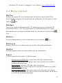
1
ArborSonic 3D
Acoustic Tomograph
User’s Manual
ArborSonic 3D Acoustic Tomograph - User’s Manual - www.arborsonic.com
1 . I n t r o d u c t i o n ................................................................................................... 3
1 . 1 F u n d a m e n t a l s o f a c o u s t i c t e s t i n g ............................................ 3
2 . H a r d w a r e o v e r v i e w ................................................................................... 5
2 . 1 G u a r a n t e e .................................................................................................. 5
2 . 2 T e c h n i c a l d a t a ....................................................................................... 6
2 . 3 P i e z o t r a n s d u c e r s ................................................................................ 6
2 . 4 A m p l i f i e r b o x e s .................................................................................... 7
2 . 5 B a t t e r y b o x .............................................................................................. 8
2 . 6 S e n s o r r e m o v e r ..................................................................................... 9
3 . F a k o p p 3 D S o f t w a r e ............................................................................... 10
3 . 1 R e q u i r e m e n t s ........................................................................................ 10
3 . 2 I n s t a l l a t i o n ............................................................................................ 10
3 . 3 I n t r o d u c t i o n .......................................................................................... 10
3 . 4 M e n u s y s t e m ......................................................................................... 12
3 . 5 T a b s ............................................................................................................. 13
3 . 5 . 1 N o t e s .................................................................................................. 13
3 . 5 . 2 T i m e D a t a ....................................................................................... 14
3 . 5 . 3 T i m e m a t r i x .................................................................................. 15
3 . 5 . 4 P o s i t i o n d a t a ................................................................................ 16
3 . 5 . 5 D i s t a n c e m a t r i x .......................................................................... 19
3 . 5 . 6 V e l o c i t y m a t r i x .......................................................................... 19
3 . 5 . 7 V e l o c i t y m a p ................................................................................ 20
4 . F a k o p p M u l t i l a y e r V i e w e r ................................................................. 23
4 . 1 R e q u i r e m e n t s ........................................................................................ 23
4 . 2 I n s t a l l a t i o n ............................................................................................ 23
4 . 3 U s a g e .......................................................................................................... 23
5 . U s i n g F a k o p p 3 D ...................................................................................... 27
5 . 1 S e t t i n g u p t h e h a r d w a r e ............................................................... 27
5 . 2 S e t t i n g u p t h e B l e t o o t h c o n n e c t i o n ..................................... 30
5 . 3 C o l l e c t i n g t i m e d a t a ....................................................................... 38
5 . 4 I n t e r p r e t i n g t h e r e s u l t s ................................................................. 39
5 . 5 T a k i n g a p a r t .......................................................................................... 40
6 . C o n t a c t s .......................................................................................................... 41
2
ArborSonic 3D Acoustic Tomograph - User’s Manual - www.arborsonic.com
1. Introduction
ArborSonic 3D is designed to evaluate trees, logs and lumber. The equipment is able
to detect holes, decay and cracks in trees by a nondestructive technique. ArborSonic
3D measures the transit time of the stress wave between transducers. The equipment
helps the forester to determine the optimal time for wood felling. Other important
applications are the determination of residual strength of old timbers and the
evaluation of the stiffness of logs.
1.1 Fundamentals of acoustic testing
Testing by tapping is an ancient technique. The woodpecker taps trees and in this way
it is able to find insects under the bark. Physicians also examine by tapping the human
body. The tapping technique is able to examine living trees as well.
The woody material of a healthy tree is a good sound guide while decayed wood is a
sound absorber. The velocity of sound in healthy wood is much higher than in voids or
in decaying wood. This is the reason why the sound avoids defects in the tree.
As stated above, ArborSonic 3D measures the time of sound traveling from one sensor
to another. If there is a hole between the two sensors, the sound can not pass through
the hole and has to travel a longer distance which means a higher traveltime.
ArborSonic 3D uses several sensors and measures the traveltimes between each sensor
pair. In this way internal holes can be mapped.
Figure 1 Sound path in healthy and decayed tree
3
ArborSonic 3D Acoustic Tomograph - User’s Manual - www.arborsonic.com
Figure 2 Holes can be found with time
measured along several lines
4
ArborSonic 3D Acoustic Tomograph - User’s Manual - www.arborsonic.com
2. Hardw are overview
ArborSonic 3D consists of the following hardware parts:
Piezo transducers
Amplifier boxes
Battery box
Cables to connect amplifier boxes and battery box
Caliper for measuring sensor positions
Sensor remover tool
Tape measure
Steel hammer for tapping transducers
Rubber hammer for fixing transducers
Case
Figure 3 Contents of the ArborSonic 3D case
2.1 Guarantee
The ARBORSONIC instrument, including the sensors, is guaranteed for one year. The
guarantee starts on the date displayed on the bill and is valid for the following one
year. Any repair should be sought from the manufacturer. The guarantee does not
cover any breakage caused by misuse or deliberate damage to the instrument.
5
ArborSonic 3D Acoustic Tomograph - User’s Manual - www.arborsonic.com
2.2 Technical data
Total weight incl. case without PC
Battery supply:
Power consumption per amp. box
Instrument case:
Low battery indicator:
Standard deviation of time:
Sensor (start and stop):
RS232 baud rate is fixed:
Databit
Parity
Stopbit
Connection to PC
Permissible temperature range for
use and storage:
8 kg
9V rechargeable battery
60 mW
Peli Case
led
± 2 µs
high sensitivity accelerometer
9600 bps
8
none
1
Bluetooth
0-40°C
2.3 Piezo transducers
One of the most important part of the ArborSonic 3D system are the special piezo
transducers. These transducers can be fixed by the integrated nail on the trunk and can
stand hammer taps so they are very robust. On the other hand the noise-level is very
low allowing for precise measurements.
Figure 4 Piezo transducer with integrated nail
6
ArborSonic 3D Acoustic Tomograph - User’s Manual - www.arborsonic.com
2.4 Amplifier boxes
The sensors are connected to the amplifier boxes with BNC connectors. The sensors
and the connectors on the amplifier boxes are numbered as well, however because the
sensors are identical, you can use any sensor with any amplifier box. The only thing
that matters is the numbering of the connectors, because the system identifies the
measured traveltimes based on this numbering.
There are cables to connect the amplifier boxes. Make sure to apply correct connector
position when connecting as shown on figure. Connect neighbouring amplifier boxes
with the bottom connector of the one box and the side connector of the other box.
Every amplifier box has to be connected to another one.
Figure 5 Apply correct connector positioning
Figure 6 Connect bottom to side
7
ArborSonic 3D Acoustic Tomograph - User’s Manual - www.arborsonic.com
2.5 Battery box
The battery box contains the battery for the system. It has to be connected with the
amplifier boxes, can be connected to any amplifier box, but it is advised to connect it
to the first or last box. There is an ON-OFF switch on the battery box. Keep it turned
off while connecting each component and turn it only on when you start the
measurement. When turned on, you can use the yellow battery checker button which
lights the green led when the battery is OK. Otherwise please change the battery. We
recommend to use a 9V rechargeable battery. Please make sure to apply correct
polarity as shown in the battery container when replacing battery, otherwise the
amplifiers may be damaged. Always keep the unit turned off while changing battery.
The battery box also contains the Bluetooth converter for PC connectivity.
Figure 7 Battery box with ON-OFF switch and battery checker button
Figure 8 Bottom side of battery box for battery replacement.
Always apply correct polarity when changing battery.
8
ArborSonic 3D Acoustic Tomograph - User’s Manual - www.arborsonic.com
2.6 Sensor remover
There is a special tool for removing sensors from the tree. Just attach it to the sensor
and use the weight a couple of times to pull the sensor out. Don’t use this tool to drive
the sensor in.
Figure 9 Sensor remover
9
ArborSonic 3D Acoustic Tomograph - User’s Manual - www.arborsonic.com
3 . A r b o r S o n i c 3 D S o ft w a r e
The traveltimes measured by ArborSonic 3D are transmitted to the software on the
PC. This software calculates the resulting 2-dimensional velocity map of the internal
state of the tree.
3.1 Requirements
-
Windows Vista, XP or 2000 system
10MB free space on your hard disk
CD drive
RS232 port or properly installed USB-RS232 converter cable or Bluetooth
3.2 Installation
To install the software, just run the installer from the CD provided. The installer will
ask for the destination directory and copy the program files. When finished, you can
start the program from the Start Menu.
3.3 Introduction
This program collects end evaluates data from the ArborSonic 3D to PC. It operates
for sensor numbers between 6 and 64. The time data is collected on the RS232 port,
distance data manually through the keyboard. The result is a 2 dimensional velocity
map representing the internal state of the tree. The measurement can be saved to a file
to re-open and re-evaluate later.
The program can be started with the ArborSonic3D.exe, or simply by clicking the
“ARBORSONIC 3D” icon
on your desktop or in the Start Menu. The program
window consists of 3 parts: On the top the menu line and 4 icons below it. The main
area of the window consist of 7 tabs, these are responsible for the data inputs and
evaluation. On the bottom there is a status bar.
10
ArborSonic 3D Acoustic Tomograph - User’s Manual - www.arborsonic.com
The menu system is the following:
-
-
-
File
o
o
o
o
o
Export
o
o
o
o
Help
o
o
New
Open
Save
Save as
Exit
Measurement as HTML
Map as image
Map as data file
Intersection as data file
Help
About
The 7 tabs are:
-
Notes
Time data
Time matrix
Position data
Distance matrix
Velocity matrix
Velocity map
11
ArborSonic 3D Acoustic Tomograph - User’s Manual - www.arborsonic.com
3 .4 M e nu s ys t e m
File/New
Prepares the program for a new measurement, all previous unsaved data will be
deleted. Before it happens, the program asks for confirmation. It is the same as if you
click the
icon.
File/Open
Opens a previously saved measurement. The default extension for ArborSonic3D
measurement files is *.f2d. The program asks for confirmation before the current
unsaved data gets overwritten on the data fields. It is the same as if you click the
icon.
File/Save
Saves the measurement to a file. It is the same as if you click the
icon.
File/Save as
Same as File/Save except that you can save the file with a different filename.
File/Exit
Exits the program. If there are unsaved data, asks for confirmation.
Export
You can export the test results in 3 different forms:
-
-
Measurement as HTML file: export, where the notes, measured time,
geometry information, time, distance and velocity matrices are available
including the image result.
Map as Image: generates a JPG file of the velocity map.
Map as data file: the velocity map can be exported as a matrix to an ASCII
file for further processing.
Intersection as data file: a line intersection can be selected on the velocity
map. This function saves the velocity values versus the distance on the line to
an ASCII file for further processing.
12
ArborSonic 3D Acoustic Tomograph - User’s Manual - www.arborsonic.com
The
and
icons start and stop the serial communication. They are useful for
example if you use a Bluetooth RS232 adapter and it was turned off when the program
started, so the program could not build up the connection at the beginning. Clicking
the disconnect and connect icon in this case can build up the connection. You can
always see the list of opened COM ports in the status bar.
3.5 Tabs
The main screen of the program is divided into 7 tabs. To complete a measurement, go
through each of these tabs and provide the necessary information.
3.5.1 Notes
Figure 10 The notes tab
Channels: number of sensors your ArborSonic3D actually has.
13
ArborSonic 3D Acoustic Tomograph - User’s Manual - www.arborsonic.com
Com port: number of RS232 port your ArborSonic3D uses to connect to PC. You can
set a specific port number between COM1 and COM99. You can also set the port
selection to AUTO. In this case the program tries to open all the ports from COM1 to
COM99. The advantage of AUTO is, that you don't have to know the exact port
number, you only have to connect the unit. The disadvantage is, that the program
opens and therefore allocates all other ports also, but we recommend to use this
setting. On the status bar if Time data tab is active you can see which ports could been
opened. Please note, that serial communication is only active if Time data or Time
matrix tab is selected. You can read more about serial communication
Species: Choose the species of the tree in the Species field. The tree species database
is stored in the species.dat and speciesname.dat. The results depend on the chosen
species. The measured velocity has to be corrected because of the deviation between
the radial and tangential velocity. Software calculates the radial velocity – even if the
velocity measurement has been done in tangential orientation.
Additional notes: you can enter here any kind of comment about the measurement
3.5.2 Time Data
You can see the data coming in from the serial port on this tab. After you hit a sensor,
ArborSonic3D measures the wave propagation time to all the other sensors and sends
the measured data to the PC. The table in the middle of this tab stores these data. The
column number in the table matches the sensor number. The leftmost column of the
table doesn't contain time data, but it refers to the quality of each row, it can have one
of the following values: OK, Invalid or Filtered.
A row is indicated as OK, if it contains exactly one piece of 0 time. Otherwise it is
indicated as Invalid and will not be used during the evaluation process. All the time
data lower than 10 microsec (this value can be changed in fakopp2d.ini, zerolimit) is
stored as 0. Also from the disconnected sensors the program reads 0.
During the data reading there is a filtering algorithm (can be turned off by the
checkbox) that tries to filter the data rows with high standard deviation. It starts
filtering if there are at least 3 OK data rows from a specific sensor. If there is a
difference more than 80 microsecond between any data from the same sensor, the
algorithm selects the most deviating row as Filtered. Filtered rows will not be used
during the evaluation process.
The list on the left of this table shows the number of OK hits to every sensor. At least
3 OK rows are needed from every sensor (this value can be changed in fakopp2d.ini,
minhit). The cell of a row is red if there in not yet enough data. You can delete the
selected data row with the Delete selected button. The last measured line can be
14
ArborSonic 3D Acoustic Tomograph - User’s Manual - www.arborsonic.com
deleted with the Delete last button. The Delete invalid button deletes all the Invalid
rows.
The Clear button deletes all the data at once. During the data collection phase it is
highly recommended to observe the collected data and delete the ones with high
deviation if they are not filtered out automatically. 1-2% deviation between the data
rows can be accepted.
Figure 11 The time data tab after collecting the time data
3.5.3 Time matrix
If there are enough data rows from each sensor, then in this table you can see the
average propagation times between each sensor pair and the standard deviation
between the [] signs. It is highly recommended to check these standard deviation
valueas at each measurement and if you experience high values (above 3%), then go
back to time collection and remove or re-measure some lines.
The standard deviation between the [] signs can be absolute, I this the unit is
microseconds, or it can be relative to the measured average, in this case the unit is
percent. You can switch between these two formats by clicking on the “Standard
deviation in %”.
The time matrix contains the average measured time and the standard deviation.
15
ArborSonic 3D Acoustic Tomograph - User’s Manual - www.arborsonic.com
You can also check here the time difference between the travel time measured in the 2
different directions. The row number of a given cell is the number of sensor hit (start
sensor), the column number is the number of stop sensor. So normally you should get
approximately the same average in the i.th row and j.th column as in the j.th row and
i.th column. If the difference is too high, it can mean that the sensor with higher
average times is not correctly fastened into the tree or it is out of order. If the
difference is greater than 80 microsec (this value can be changed in fakopp2d.ini,
devlimit2), then the program shows a notification.
Figure 12 The time matrix tab during the evaluation.
3.5.4 Position data
You can set the position of the sensors on this tab. You can choose between three
distance templates: Ellipse, Irregular and Longitudinal. In case of Ellipse and Irregular
the transducers are arranged in a single plane on the tree, in Longitudinal case the
transducers are in two planes, see more about this below.
In any case if you are typing the desired distance data, you can move between the
input cells with up/down arrow or the Enter button.
16
ArborSonic 3D Acoustic Tomograph - User’s Manual - www.arborsonic.com
All the distances are in cm.
Ellipse is recommended if the shape of tree is approximately circular or elliptical. In
this case you only have to measure 3 distances: D1 and D2 are the small and large
diameters (perpendicular) of the tree, C is its circumference. After you enter every
data a message appears that contains the distance from the 1st sensor along the
circumference. Place the 1st sensor to one end of the greater diameter, this is the 0
distance. Place all the other sensors to the distances calculated by the program in
clockwise order.
If the shape of the tree trunk is too far from ellipse (D2>2*D1 or C is not the same as
the circumference of an ellipse with D1 and D2 diameters within 15%), you get an
error message.
Figure 13 The ellipse geometry model
Choose Irregular if the shape of tree is not elliptical. In this case you have to measure
(2n-3) distance data, where n is the number of sensors. First place the sensors on the
tree in a plane in clockwise order as you like, but try to keep roughly equal distances
between the sensors. After this you have to measure the distance between the given
sensor pairs. Make sure to type the distance to the correct input field, otherwise the
program will go wrong. The program calculates the coordinates of the sensors from
17
ArborSonic 3D Acoustic Tomograph - User’s Manual - www.arborsonic.com
these data and the image appears, you can use this image to check if the data you
entered was correct.
There is one additional input parameter for both position schemes at the bottom of the
list, this is the Penetration Depth or PD parameter. This is the depth at which the
sensor needles are driven inside the tree from the bark surface. It is necessary, because
when you register the geometry, you measure positions at the bark surface, however
the real propagation of sound starts from the end of the needles. The normal value for
this parameter is 3 cm, but for normal size trees (above 50 cm diameter) this value is
not critical. However, in case of small trees, it is important to enter this parameter
correctly.
Figure 14 The irregular geometry model.
18
ArborSonic 3D Acoustic Tomograph - User’s Manual - www.arborsonic.com
3.5.5 Distance matrix
After every distance data is entered on the position tab, you can check all the distances
in the Distance Matrix. The applied unit is cm.
Figure 15 The Distance Matrix.
3.5.6 Velocity matrix
There is a table on this tab containing the calculated velocities between each sensor.
Because of the time correction (M in the Position Tab, and the Species settings on the
Notes tab) the velocities in the table are not exactly the ratio of distance and measured
time. 90% of the average of of the selected (green background) velocities is used to
calculate the Reference Velocity. The Reference Velocity will be the Vmax value on
the Velocity Map. You can change the format of the shown velocities to percentage by
clicking on the “Show Relative Velocity” button. Clicking it again will change it back
to m/s.
19
ArborSonic 3D Acoustic Tomograph - User’s Manual - www.arborsonic.com
Figure 16 Velocity Matrix and the values selected to determine Reference
Velocity
3.5.7 Velocity map
The result is a 2-dimensional velocity map of the tree.
If there are enough time and distance data, the program calculates the velocity map in
1 or 2 seconds. On the left you can see the color scale. You can choose between
several color scales from Color template field. Vmin and Vmax mean the minimal and
maximal velocities regarding to the colors. You can change them with the + and buttons by 50 m/s steps or type another value into the edit box. The default value of
Vmax comes from the reference velocity. If you move the cursor over the map, the
velocity of the pixel under the cursor appears. The velocity map contains radial
velocities.
There are 3 visualization modes.
3D map shows the velocity map as a 3D surface. With the left mouse button clicked
you can rotate the surface. The coordinates and velocity at the mouse cursor is
displayed in a box. With the right mouse button clicked you can select a line
intersection of the map. This intersection can be exported to file in the Export menu.
20
ArborSonic 3D Acoustic Tomograph - User’s Manual - www.arborsonic.com
2D map shows the same map, the only difference is that it is shown in 2D and only
colors represent the velocity differences. A line intersection can also be selected with
the right mouse button.
Graph mode displays not the reconstructed interval velocity distribution, but the
measured velocity values between the sensors. The color of the lines corresponds for
the velocity values. Moving the mouse over the lines display the line velocity.
The velocity map has two imperfections.
The sound velocity in a hole inside the tree is same as in the air, 340 m/s but the
measured velocity will be remarkably higher. This is because the waves by-passes the
hole and therefore there is no method to measure the exact velocity inside a hole.
Generally, if the velocity decreases somewhere under 90-85% of the average velocity,
then there can be a hole or decay.
The other problem is that if there is a long narrow crack in the tree then it shadows the
nearby area and the result will not show a narrow crack but a much smaller and wider
area at the boundary.
The real resolution of the image depends of the number of sensors used. With 8
sensors you can detect any decay greater than 5% of the whole cross-sectional area.
With 32 transducers this ratio is 2%.
Figure 17 Velocity map visualization in 3D mode
21
ArborSonic 3D Acoustic Tomograph - User’s Manual - www.arborsonic.com
Figure 18 Velocity map visualization in 2D mode
Figure 19 The velocity lines
22
ArborSonic 3D Acoustic Tomograph - User’s Manual - www.arborsonic.com
4. ArborSonic Multilayer View er
If you create measurements of a single tree at several heights, it can be useful to show
the results on a single image in three dimensions. The ArborSonic Multilayer Viewer
solves this problem and assembles 2D images into a 3D reconstruction of the tree.
4.1 Requirements
-
Windows 2000 or higher
2MB free space on your hard disk
.NET Framework v2.0 or later
4.2 Installation
This software is installed along with the ArborSonic 3D software.
4.3 Usage
ArborSonic Multilayer Viewer assembles ready measurements in .f2d files together.
All measurements have to be with same sensor number and tree species. To add a new
layer, click the
button in the toolbar. You can change the display name
of the layer and most importantly set the layer height from the ground in centimeters.
You can later modify the layer options with the
with the
icon. Any layer can be deleted
icon.
23
ArborSonic 3D Acoustic Tomograph - User’s Manual - www.arborsonic.com
Figure 20 Enter layer height when adding new layer
After adding several layers at several heights, you can choose between two view
modes.
You can view each single layer, just like in the ArborSonic 3D software by selecting
the layer itself from the layer list. You can switch between 2D and 3D view mode with
the
icon.
Figure 21 Single layer view mode in 2D
To view the assembled 3D structure, select the project name (topmost element) from
the layer list. You need to have at least 2 layers added for this mode to work.
24
ArborSonic 3D Acoustic Tomograph - User’s Manual - www.arborsonic.com
Figure 22 Multilayer view mode without cutting plane
In multilayer view mode a vertical cutting plane can be inserted between the layers.
This plane shows interpolated values of the two layers. The plane is always in the
middle of the layers and faces the viewer. You can turn on the cutting plane with the
icon.
Figure 23 Multilayer view mode with cutting plane
25
ArborSonic 3D Acoustic Tomograph - User’s Manual - www.arborsonic.com
Each view can be rotated with the mouse. The color template and velocity limits can
be changed the same way as in the ArborSonic 3D software.
A project can be saved with the
icon or saved with a new name with the
An existing project can be loaded with the
started with the
icon. Use the
icon.
icon or a totally new project can be
icon to get some help.
26
ArborSonic 3D Acoustic Tomograph - User’s Manual - www.arborsonic.com
5 . U s i n g Ar b o r S o n i c 3 D
This section describes practical knowledge, tips and tricks for using the ArborSonic
3D system.
5.1 Setting up the hardw are
When going to a new tree, find a relatively clear spot for the case. Examine the tree
and select the height where you would like to do the measurement and decide if the
tree looks elliptical of irregular.
PC or
Laptop
1
8
1
2
2
Battery
unit
7
3
7
8
6
4
5
3
4
5
6
The first step is to attach the sensors. Use the rubber hammer for this purpose. The nail
has to penetrate the bark and a good coupling is very important between the nail and
the wood material, so the sensors have to be so tight that you can not rotate them with
27
ArborSonic 3D Acoustic Tomograph - User’s Manual - www.arborsonic.com
3 outstretched fingers. Coupling is so important, that if you notice later, when tapping
the sensors with the steel hammer that a sensor moved more inside the tree and was
not coupled good enough, you have to fix it with the rubber hammer and start with
tapping all the sensors from the beginning again.
If you choose irregular position mode, you can place the sensors as you like, roughly
the same distance is advised between the sensors, but it is not a requirement. When
you are ready, you have to measure the distances with the caliper between those
sensor pairs which the software asks for.
If you choose ellipse position mode, you need to fix the first transducer at one end of
the large diameter of the tree. Fix the tape around the tree with this only sensor as
shown on the image below. Measure the large and small diameters of the tree with the
caliper and enter these data along with the circumference to the software. The software
will calculate the position of each sensor along the tape on the trunk. Make sure to
remove the line after placing the sensors because steel can act as an acoustic
conductor.
Figure 24 The way to fix the tape with the first transducer
28
ArborSonic 3D Acoustic Tomograph - User’s Manual - www.arborsonic.com
Figure 25 Sensors with tape around the trunk
The sensors need to be placed on a plane perpendicular to the grains. So if the tree is
bent, this plane will not be parallel to the ground, but tilted to the same angle as the
tree is bent.
The next step is to connect the amplifier boxes to the sensors with the BNC
connectors. Make sure not to cross a cable and connect the correct amplifier channels
to the correct sensors because it can mess up your whole measurement. The sensors
are numbered as well, but they are identical so they can be interchanged.
After the amplifier boxes are connected to the sensors you need to connect the
amplifier boxes with each other with the cables provided. Connect neighbouring boxes
with the bottom connector of one box and the side connector of the other and make
sure to apply correct connector positioning as explained in section 2.2. When you are
ready connecting the amplifier boxes, you can connect the battery box, but keep it
turned off while connecting. You can connect it to the first or the last amplifier box as
well.
29
ArborSonic 3D Acoustic Tomograph - User’s Manual - www.arborsonic.com
5.2 Setting up the Bletooth connection
To connect your PC to ArborSonic 3D, you need to set up the Bluetooth connection in
Windows. This process is explained here step by step for Windows XP, but it is
almost the same for other Windows versions.
Step 1: Go to the Control Panel and select Bluetooth, double-click it.
Step 2: Click add.
30
ArborSonic 3D Acoustic Tomograph - User’s Manual - www.arborsonic.com
Step 3: Select My device is set up and ready to be found and click Next. Make sure to
turn the battery box on before clicking next. The green led should light if you press the
yellow button on the battery box. Otherwise the battery should be recharged.
Step 4: Wait until the system finds the converter. If the converter can not be found
make sure again that the battery box is turned on and that your Bluetooth receiver in
your PC is installed properly.
31
ArborSonic 3D Acoustic Tomograph - User’s Manual - www.arborsonic.com
Step 5: If everything works fine, you should see the converter in the list. Select it and
click Next. If Windows can not find your device, try turning Fakopp 3D off and on
again and search again.
Step 6: Select the Use the passkey found in the documentation and type 1234. Click
Next.
32
ArborSonic 3D Acoustic Tomograph - User’s Manual - www.arborsonic.com
Step 7: See as the system sets up the converter.
Step 8: On the final page you can find the COM port numbers. The ArborSonic
software can find these numbers automatically for you, so you don’t need them, unless
you want to test the communication with the HyperTerminal program for Windows.
Click Finish.
33
ArborSonic 3D Acoustic Tomograph - User’s Manual - www.arborsonic.com
Step 9: This is the screen you should see after the successful setup.
Step 10: To test the connection, start the HyperTerminal in Star / Programs /
Accessories / Communication / HyperTerminal. At the start it asks for some telephone
numbers because this program was also used for modem connections; just press cancel
and yes on the first two screens.
34
ArborSonic 3D Acoustic Tomograph - User’s Manual - www.arborsonic.com
Step 11: Give a name to the connection, just any name, it does not matter. Let’s say
f2d.
Step 12: In the COM port list you have to select the outgoing port and click OK.
35
ArborSonic 3D Acoustic Tomograph - User’s Manual - www.arborsonic.com
Step 13: Click the Call icon to start the connection. If it is possible to connect to the
selected COM port, the Bluetooth window should also signalize the connection.
Otherwise try to select a different COM port.
Step 14: Tap a couple of times at any of the sensors to generate some data traffic. You
should have the raw transmitted data on your screen. Now you can be sure that the
communication between ArborSonic 3D and the PC works fine.
36
ArborSonic 3D Acoustic Tomograph - User’s Manual - www.arborsonic.com
Step 15: Start the ArborSonic 3D software, but don’t forget to close HyperTerminal,
otherwise the com port will be blocked and you can not get anything in the
ArborSonic 3D software. Set the number of sensors (channels) you have and select
Auto in the COM port list. You can also select the same COM port which worked in
HyperTerminal, however the Auto mode is recommended because it opens every
COM port in the same time and you don’t have to know the exact port number. The
list of opened COM ports is in the status bar at the bottom. You always have to make
sure that no other program (HyperTerminal, another running ArborSonic 3D software
or anything) uses the COM port.
Step 16: Go to the Time Data tab and tap a couple of times at the sensors. You should
see your data arriving. You can always break and rebuild the connection with the
connect/disconnect icons at the top, so you don’t need to restart the program. The
number of COM port where the last data arrived from is in the status bar at the bottom.
37
ArborSonic 3D Acoustic Tomograph - User’s Manual - www.arborsonic.com
Step 17: Finally, if the communication does not work at any stage, use the standard
method for solving IT problems: turn off the ArborSonic 3D hardware, close every
program and remove the converter from the Bluetooth device list, you can even restart
your PC. Turn on the ArborSonic 3D hardware again, re-install the converter based on
this tutorial and try to get the data again.
5.3 Collecting time data
To get the
ArborSonic
ArborSonic
software. If
sound wave traveltimes between the sensors, you need to start the
3D software after setting up the bluetooth connection. Turn on
3D with the switch on the battery box and start the ArborSonic 3D
you forgot to turn on ArborSonic 3D before you started the software, no
problem. Just click the
icon in the toolbar to disconnect and click the
icon to
connect again. If you still have the Bluetooth Devices window open (see the image of
Step 13 of chapter 6.2), you should see the “Connected” status appear there. If you
would like to switch off ArborSonic 3D while still using the software, you can do it
without any problems, but in case you switch it on again, use the
and
icons to
rebuild the connection.
It is recomended to keep the COM port on AUTO, otherwise you need to know the
exact port number.
If everything looks fine, you can switch to Time data tab and start tapping the sensors.
A good tap is:
- in the direction of the sensor needle
- at the center of the sensor
- with uniform power
- hammer speed is relatively high
- hammer springs immediately back from the sensor head
- at least 1 second between two taps
Bad taps are:
- on the side of the sensor
- with very low or non-uniform power
- hammer remains on the sensor head after tapping
38
ArborSonic 3D Acoustic Tomograph - User’s Manual - www.arborsonic.com
If you make a bad tap, delete it immediately from the time data list with the Dele Last
button. Be careful not to tap on the cable connecting point or on the cable because it
will damage the sensor.
At least 3, but possibly 5 taps are recommended per sensor. When you tapped all the
sensors, examine the collected data and compare rows from the same sensors. Up to
3% deviation is acceptable, but if you find a line to be deviated from the others too
much, select and remove it with the Delete Selected button. If a sensor is not coupled
tight enough to the wood, you may see greater deviations. There is a built-in filtering
for this purpose which you can use by ticking the Auto Filter checkbox which labels
some lines with ‘Filtered’ and these lines will be excluded from the evaluation.
However, it is recommended to do this check and filtering manually as well.
When your batteries are getting tired, you may start receiving 28 microseconds on any
sensor. This is definitely bad data which will damage your whole measurement so
delete lines containing 28s.
You can check the average time deviations after the ± sign in the Time Matrix tab. If
you find some values too high (above 3%), go back to the Time Data tab and review
the data received from / to those sensors. On the left of the time matrix there is a list
labeled with dT. This includes the average deviations of times measured when a
sensor was tapped (start) and when it received the sound wave (stop). If this deviation
is too high, it can also indicate bad coupling.
5.4 Interpreting the results
When enough time data are collected and the sensor positions are registered correctly,
you can move to evaluation on the Velocity Map tab. You are free to choose between
2D and 3D visualization of the interval velocity distribution.
The velocity map has two imperfections.
The sound velocity in a hole inside the tree is same as in the air, 340 m/s but the
measured velocity will be remarkably higher. This is because the waves by-passes the
hole and therefore there is no method to measure the exact velocity inside a hole.
Generally, if the velocity decreases somewhere under 90-85% of the average velocity,
then there can be a hole or decay.
The other problem is that if there is a long narrow crack in the tree then it shadows the
nearby area and the result will not show a narrow crack but a much smaller and wider
area at the boundary.
39
ArborSonic 3D Acoustic Tomograph - User’s Manual - www.arborsonic.com
The real resolution of the image depends of the number of sensors used. With 8
sensors you can detect any decay greater than 5% of the whole cross-sectional area.
With 32 transducers this ratio is 2%.
5.5 Taking apart
When you are ready with the measurement, the parts of the system can be removed on
a backward way. So first turn off the battery box, remove the cables between the
amplifier boxes, remove the sensors from the amplifier boxes and finally remove the
sensors. Please note that if you make another measurement nearby and don!t would
like to take apart all cable connections, you still need to disconnect the sensors from
the amplifier boxes before pulling out the sensors from the tree, otherwise the
connectors may be damaged.
To deattach the sensors from the tree you have two possibilities. First, you can use the
sensor remover which is a very convenient way. Just attach the remover to the sensor,
use the weight a couple of times and the sensor is out.
The other method is the manual method. Grab a sensor so that the sensor head is in
your palm and hold the cable connecting point (but not the cable!) with your fingers.
Start rotating the sensor around the needle there and back and pull it in the same time
while rotating. In this way the can be pulled out.
Don’t use the hammer handle as a support under the cable connecting point to pull the
sensor out, because this applies a sideway force to the needle which can bend or break
it on the long run. Be very careful not to damage the cable during the process.
40
ArborSonic 3D Acoustic Tomograph - User’s Manual - www.arborsonic.com
6 . C o n ta c ts
If you have any question or problems, don’t hesitate to contact us.
Fakopp Bt.
Address:
Fenyo u 26
H-9423, Agfalva
Hungary
Website: www.fakopp.com
E-mail: [email protected]
Tel: +36 99 510 996
Fax: +36 99 33 00 99
41