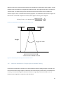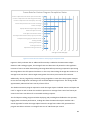
1
Multirotor Unmanned Aerial Vehicle Autonomous Operation in an Industrial Environment using On-‐ board Image Processing Christopher Venables 20496617 Faculty of Engineering, Computing and Mathematics University of Western Australia Supervisors: Prof. Dr. Thomas Bräunl Mr Chris Croft Final Year Project Thesis School of Electrical, Electronic & Computer Engineering University of Western Australia 1st November 2013 Abstract This project aimed to expand on multirotor unmanned aerial vehicle autonomous capabilities through the use of on-board image processing, in outdoor, unmapped environments. This capability would simplify multirotor unmanned aerial vehicle operation and expand on the commercial applications within industrial environments. A multirotor unmanned aerial vehicle was assembled and algorithms and programs were successfully implemented allowing autonomous navigation of GPS waypoints and coloured object tracking using on-board image processing. A remote browser interface was also developed to allow new mission data to be uploaded to the vehicle while carrying out autonomous objectives. The multirotor unmanned aerial vehicle was successfully able to detect and autonomously track a target object by using on-board image processing. Due to the on-board computational limitations enforced by a limited payload, the complete autonomous target object tracking program operates at an average frame rate of 2.85 fps and is capable of reliably tracking a person moving at speeds of up to 10 m/s. This project has demonstrated the validity of on-board image processing for autonomous multirotor unmanned aerial vehicle control with a robust system that is capable of successfully operating in an outdoor, industrial environment. With increased computational power and by modifying the image processing algorithms for the desired tracking target, this system may be suitable for commercial applications including search and rescue, security and policing, data collection and aerial photography and filmography. ii Acknowledgements I would like to thank my supervisor Professor Dr. Thomas Bräunl for enabling this research program and providing extensive advice and encouragement to improve this project. I would also like to thank my external supervisor, Chris Croft, for his funding contribution to enable this project and for his constant advice and enthusiasm. I would also like to thank my project group member, Rory O’Connor, for his assistance and input into the success of this project. I would also like to thank the contributors and authors of the open source libraries and packages that have been used to complete this project, particularly Raspivid, OpenCV and Servoblaster. Finally, I would like to thank my friends and family for their ongoing support and encouragement throughout this project and my entire time at The University of Western Australia. iii Table of Contents ABSTRACT _________________________________________________________________ II ACKNOWLEDGEMENTS _____________________________________________________ III 1 2 3 INTRODUCTION _________________________________________________________ 1 1.1 OBJECTIVES __________________________________________________________ 2 1.2 ENGINEERING DESIGN CRITERIA _____________________________________________ 2 1.3 PROCESS ____________________________________________________________ 4 LITERATURE REVIEW _____________________________________________________ 5 2.1 ATTITUDE CONTROL _____________________________________________________ 5 2.2 ON-BOARD IMAGE DATA CAPTURE ___________________________________________ 8 PROCESS _____________________________________________________________ 12 3.1 MULTIROTOR COMPONENT SELECTION _______________________________________ 12 3.2 MULTIROTOR ASSEMBLY _________________________________________________ 16 3.3 LAWS, REGULATIONS AND RELEVANT STANDARDS ________________________________ 17 3.4 AUTOMATION ________________________________________________________ 19 3.5 AUTONOMOUS CONTROL SYSTEM __________________________________________ 24 3.6 AUTOMATION ALGORITHMS ______________________________________________ 30 3.7 CONTROL INTERFACE ___________________________________________________ 61 3.8 REMOTE BROWSER INTERFACE _____________________________________________ 65 3.9 LOG FILE ___________________________________________________________ 66 3.10 ISSUES AND DIFFICULTIES ________________________________________________ 68 4 5 EXPERIMENTS _________________________________________________________ 73 4.1 IMAGE PROCESSING FRAME RATE TESTS ______________________________________ 73 4.2 ANGLE OF VIEW ______________________________________________________ 77 4.3 OBJECT TRACKING ALGORITHM TESTING ______________________________________ 77 4.4 GPS WAYPOINT NAVIGATION ACCURACY _____________________________________ 78 RESULTS AND DISCUSSION _______________________________________________ 79 5.1 IMAGE PROCESSING FRAME RATE RESULTS _____________________________________ 79 iv 5.2 ANGLE OF VIEW ______________________________________________________ 85 5.3 COLOUR BLOB DETECTION ALGORITHM _______________________________________ 89 5.4 OBJECT TRACKING ALGORITHM ____________________________________________ 90 5.5 GPS WAYPOINT ALGORITHM ____________________________________________ 100 5.6 SAFETY ___________________________________________________________ 101 5.7 COMMUNITY WORK __________________________________________________ 101 6 APPLICATIONS ________________________________________________________ 101 6.1 SEARCH AND RESCUE __________________________________________________ 102 6.2 POLICING __________________________________________________________ 102 6.3 SPORTING EVENT AERIAL FILMOGRAPHY _____________________________________ 103 6.4 GROUND ROBOT COMMUNICATIONS LINK ____________________________________ 104 6.5 INTERFACULTY DISCUSSIONS _____________________________________________ 104 6.6 LIMITATIONS________________________________________________________ 104 7 CONCLUSION _________________________________________________________ 105 8 FUTURE WORK AND RECOMMENDATIONS _________________________________ 108 9 REFERENCES _________________________________________________________ 109 10 APPENDICES ________________________________________________________ 118 APPENDIX A – CONTROL SIGNAL WIRING DIAGRAM ___________________________________ 118 APPENDIX B – RISK ANALYSIS __________________________________________________ 119 APPENDIX C – GENERALISED COMPLETE OBJECT TRACKING PROGRAM ALGORITHM ______________ 120 APPENDIX D – IMAGE PROCESSING FRAME RATE TEST DATA _____________________________ 121 APPENDIX D – ANGLE OF VIEW TESTING ___________________________________________ 123 v Table of Figures Figure 1: Quadcopter motor configuration[3] ___________________________________________ 1 Figure 2: MUAV with four visual identifying markers used by the Vicon system [7] ______________ 6 Figure 3: University of Pennsylvania's GRASP Laboratory [3] ________________________________ 7 Figure 4: ARS Electronica Outdoor Artistic Flying Formation [38] ____________________________ 8 Figure 5: Typical helicopter UAV [6] __________________________________________________ 10 Figure 6: DJI F550 hexacopter star configuration [66] ____________________________________ 14 Figure 7: Fully assembled MUAV ____________________________________________________ 17 Figure 8: Raspberry Pi[5] ___________________________________________________________ 21 Figure 9: Physical Relay Circuit ______________________________________________________ 22 Figure 10: Simplified wiring diagram _________________________________________________ 25 Figure 11: Standard Remote Control Pulse Width Modulation [4]___________________________ 27 Figure 12: Remote Control Receiver PWM Output Signals_________________________________ 27 Figure 13: Simplified GPS Waypoint Navigation Flowchart ________________________________ 31 Figure 14: Converting between an absolute bearing and a bearing relative to the MUAV's orientation ______________________________________________________________________________ 33 Figure 15: Determining current true orientation ________________________________________ 34 Figure 16: Determine current bearing using GPS data over time[2] _________________________ 37 Figure 17: Simplified colour blob tracking algorithm flowchart _____________________________ 41 Figure 18: HSV Hue colour wheel [1] _________________________________________________ 46 Figure 19: Bang-bang control algorithm visualisation ____________________________________ 54 Figure 20: How MUAV movement effects camera field of view when camera is mounted to MUAV frame __________________________________________________________________________ 57 Figure 21: How MUAV movement effects camera field of view when camera is mounted using a gimbal _________________________________________________________________________ 58 Figure 22: Relationship between angle of view and field of view ___________________________ 59 Figure 23: Compass direction distorted by electromagnetic interference _____________________ 72 Figure 24: Defined target GPS waypoints ______________________________________________ 78 Figure 25: Average program frame rate for various image resolutions for converting to an accessible OpenCV image format at full captured image resolution. _________________________________ 80 Figure 26: Average program frame rate for various image resolutions for converting to an accessible OpenCV image format and by downscaling the resolution to 426 x 320. _____________________ 81 Figure 27: Frame rate test results for various program completion states ____________________ 82 vi Figure 28: Individual frame duration for a complete object detection and tracking program, including image saving ____________________________________________________________________ 83 Figure 29: Individual frame duration for a complete object detection and tracking program, excluding image saving ____________________________________________________________________ 84 Figure 30: Horizontal field of view as a function of horizontal image resolution________________ 85 Figure 31: Vertical field of view as a function of vertical image resolution ____________________ 86 Figure 32: Dimensional angle of view as a function of dimensional image resolution ___________ 86 Figure 33: Detected colour blob image overlay _________________________________________ 89 Figure 34: Raw image captured by camera during field testing _____________________________ 89 Figure 35: GPS Latitude of Stationary Ground Target_____________________________________ 90 Figure 36: GPS Longitude of Stationary Ground Target ___________________________________ 91 Figure 37: GPS Latitude of MUAV Tracking Stationary Target ______________________________ 92 Figure 38: GPS Longitude of MUAV Tracking Stationary Target _____________________________ 93 Figure 39: Relative Horizontal Position of Detected Object within Image Frame _______________ 95 Figure 40: Relative Vertical Position of Detected Object within Image Frame _________________ 95 Figure 41: Raspberry Pi left/right control signal output ___________________________________ 97 Figure 42: Raspberry Pi forwards/backwards control signal output _________________________ 97 Figure 43: MUAV tracking a remote control car _________________________________________ 98 Figure 44: Mobile Object Tracking Test _______________________________________________ 99 Figure 45: Comparison of actual path taken vs ideal path for navigating GPS waypoints ________ 100 vii 1 Introduction The past decade has seen a significant amount of research and growing public interest into autonomous Unmanned Aerial Vehicles (UAVs). Autonomous UAVs are vehicles that are able to fly throughout an environment and complete tasks with no human interaction. UAVs can be fitted with a large variety of sensors and equipment to customise their abilities for a multitude of applications, from aerial photography and filmography [8-10] to disaster zone search and rescue [11, 12]. Autonomous UAVs can either be fixed wing aircraft (‘drones’), helicopters or multirotor helicopters. A multirotor UAV (MUAV) is an aerial vehicle with similar flight capabilities to a regular helicopter in that they are capable of moving in 3 dimensions, yawing on the spot and hovering in place [13]. Physically, the MUAV has multiple radial arms that each have a fixed position motor and propeller at the end of the arm. As the position of the motors are fixed, the vehicle is only able to move by varying the speed of each of these motors [13]. The motor configuration of a quadcopter, a MUAV with four rotors, can be seen below in Figure 1. Figure 1: Quadcopter motor configuration[3] My research will focus on MUAVs as they are simple to control at low speed and are therefore more suited to a low speed autonomous operation. Many of the previous studies into MUAV autonomy rely on off-board processing with attitude control and path planning completed at a central ground station computer. While this research has been successful, the MUAVs are unable to operate independently of the ground station processing computer. Therefore, their region of operation is 1 restricted to those areas where they are able to remain in constant communication with the ground station processing computer. A more effective autonomous solution is a fully independent selfcontained system with all data collection and processing completed on-board. Computer vision capabilities are now at the stage where on-board video cameras can be used to control and navigate a MUAV while providing dynamic environment awareness in an unknown environment [13-15]. Additionally, advances such as the Raspberry Pi [16] processor board are able to provide powerful on-board computational abilities that allow image processing and environment awareness to be carried out on board, rather than requiring a ground station computer. Complete on-board processing and sensing allows the MUAV to be able to operate in any environment. For the purposes of this research, an industrial environment is defined as a previously unseen, unknown, unmapped environment void of any specially setup equipment or visual markers. In order to be suitable for commercial application, the autonomous MUAV must be capable of operating in such an environment. Currently the autonomous capabilities of a MUAV in such an environment are limited to GPS waypoint navigation. Suitability for commercial application will be considered throughout this research as while this research does not directly lead to commercial outcomes, it is hoped that this research will provide a framework that is able to be adjusted for the specifics of a commercial objective. Furthermore, it is intended that this research demonstrates the potential capabilities of an autonomous MUAV to business and that it may lead to create awareness and potential uptake within the commercial world. 1.1 Objectives The objectives of this project are to expand upon current MUAV autonomous capabilities using only on-board sensors and on-board processing. The MUAV will detect and track a mobile target using on-board visual image processing. Additionally, this research is complementary to existing MUAV autonomous capabilities, including GPS waypoint navigation. 1.2 Engineering Design Criteria The engineering design constraints and criteria that have restricted and guided the development of this research project, in order of decreasing significance, are: Safety Cost Simplicity Portability 2 Robustness Repeatability Commercial Viability 1.2.1 Safety As a MUAV has the potential to be very dangerous and pose significant danger to the researchers, the general public and property, all measures must be taken to ensure that these risks are minimised wherever possible. The MUAV is to be tested in a controlled and private environment after each modification is made to the MUAV before being tested in the field. Additionally, any field testing must be carried out in an approved location, away from the general public and private property. At all stages of autonomy, the MUAV must be immediately be able to be switched to manual control and be able to perform a controlled self-landing when required. Safety is the most important component of this project and must be strictly observed and maintained throughout all stages of the project. 1.2.2 Cost Project funding for this research project was provided by co-supervisor Chris Croft. Overall funding was limited to approximately $3000. Effective research and planning prior to any purchasing must be undertaken to ensure that the project objectives can be effectively completed with the limited funding. 1.2.3 Simplicity The autonomous system should be simple to operate and interface with to ensure that the autonomous MUAV is able to be operated by an amateur with minimal training and experience. There should be minimal required technical setup procedures or calibration and the system should be fully operatable from a single input device. Additionally, the system should provide adequate feedback to the operator so that the MUAVs autonomous behaviour is transparent and simple to understand. 1.2.4 Portability The autonomous MUAV should be able to operate anywhere, with no lengthy setup required. All sensing equipment and data processing should be conducted on-board to ensure maximum portability. The autonomous MUAV should not require any environmental prior knowledge or special environmental preparation. The system should not be dependent on additional ground 3 control station hardware for effective operation although an optional ground control station may be used for additional operator feedback if desired. 1.2.5 Robustness The autonomous MUAV should be environmentally robust, capable of operating successfully in a range of environments. The nature and characteristics of the environment should not impact performance. 1.2.6 Repeatability The performance of the MUAV autonomous operation should be repeatable and constant, with a high success rate. The system should be effective without restriction on the tracking target’s nature or movement pattern. The system should be immune to changes in the ambient environment and be able to consistently perform in real world situations. 1.2.7 Commercial Viability While this project is purely a research project and does not have direct commercial connections, it is important that commercial viability be considered throughout the project. Care should be taken to ensure that the results of this project are applicable to commercial application. This project should increase awareness of the capabilities of MUAVs and lead to further discussions and collaborations between the university and commercial partners. 1.3 Process The project objectives of increasing the autonomous capabilities of a MUAV in an industrial environment can be separated into the following tasks: Research, purchase and assemble a MUAV Identify how to operate the MUAV autonomously Implement a GPS waypoint navigation algorithm Implement a colour blob detection algorithm Implement an object tracking algorithm Implement a target search algorithm Implement a remote access capability Evaluate success of developed system 4 There has been no previous research involving MUAVs undertaken at UWA therefore the first component of this research is to assemble a MUAV platform that will be capable of autonomous operation. The MUAV then needs to be modified to enable autonomous operation using on-board processing and control. Once the MUAV is able to be operated autonomously, a series of autonomous algorithms will be developed and tested to validate their functionality. A remote access capability will also be developed to allow the operator to interface with the UAV while in operation. Finally, the success of the developed system will be determined through extensive field testing. 2 Literature Review There is a significant amount of research that has been undertaken with direct or indirect applications to MUAV operation. The focus of this previous research is wide ranging from attitude control and stabilisation through to applications and autonomy. The public interest into MUAV capabilities and developments has also dramatically increased over the past three years [17]. The current level of public and academic interest in the MUAV field makes research into MUAVs very interesting. 2.1 Attitude Control The majority of research previously undertaken in the field of MUAVs is based on flight dynamics and attitude control systems .In standard configuration a MUAV is under actuated as it has six degrees of freedom (translation in three dimensions and rotation about three axes) and only four degrees of control (throttle, yaw, pitch and roll)[18, 19]. Therefore, the flight dynamics and attitude control systems required to allow a MUAV to operate is quite complex. Due to the complexity of the system and the costs required to research MUAV flight dynamics with real testing, many studies have focused on simulation to verify the results [19-21]. While the simulation studies assist in providing understanding the flight dynamics of the MUAV, the pure simulation environment may not always perfectly reflect reality. In simulations the MUAV control system may have access to data that is unavailable or inconsistent during an actual flight. 2.1.1 Inertial Measurement Unit Most methods of attitude control rely on data provided by an on-board Inertial Measurement Unit (IMU) [22]. A typical MUAV IMU contains a 3 axis accelerometer, 3 axis gyroscope, a 3 axis magnetometer and a barometer [22, 23]. The raw data from these sensors is non-ideal as the accelerometer suffers from noise, the gyroscope suffers from drift and the magnetometer is dependent on the local nature of the Earth’s field. Fortunately, each sensor is complementary and 5 accurate data can be reconstructed using Kalman filtering, complementary filtering or other methods [21-25]. Due to the quantity of previous research undertaken in this area, this research project will not focus on MUAV flight mechanics or attitude stabilisation and control. Instead, this research project will utilise existing MUAV attitude control methods to expand on MUAV autonomous capabilities. 2.1.2 External Sensors Alternative research into attitude control methods has utilised external sensors and external data processing either in conjunction with or instead of using an on-board IMU. The primary method of external sensor attitude control relies on visual image sensing and processing. Attitude control using external image processing requires the MUAV to be fitted with a number of distinguishable markers [7, 26-29]. Figure 2 shows an example of these visual identifying markers as used for the Vicon visual motion capture system. Figure 2: MUAV with four visual identifying markers used by the Vicon system [7] Using external visual sensors can improve MUAV attitude data accuracy and consistency [26]. Firstly, the external sensors are not subject to drift errors and provides an absolute reference [26]. Secondly, as the sensors are external to the MUAV, they are not weight restricted, can be positioned in a precisely known way and processing can be done on a powerful external computer [27]. This allows for highly accurate attitude tracking and control and also allows for advanced autonomous control of the MUAV. Studies into MUAV autonomy using external visual sensors carry out their testing in a custom designed room with all MUAV tracking and interaction computation and path planning completed at a central ground station computer [7, 27, 28, 30]. The most well-known custom designed UAV 6 development room is the General Robotics, Automation, Sensing and Perception (GRASP) laboratory at University of Pennsylvania [27], shown in Figure 3, which uses the Vicon object tracking system. The laboratory has a five metre cubed flight area that is covered by twenty Vicon MX T40 cameras is capable of capturing up to 2000 frames per second [31, 32]. ETH Zurich also has a similar facility with a ten metre cubed flight area using a similar high speed motion capture system [33]. Figure 3: University of Pennsylvania's GRASP Laboratory [3] The accuracy of the sensor data and the processing power of the processing system have allowed the autonomous MUAV to achieve advanced autonomous capabilities including balancing an inverted pendulum [34], juggling a ball between two MUAVs [35] and throwing and catching a ball as a team [36]. While this research has been successful, its reliance on expensive, specially calibrated facility does not represent the real world, industrial environment that multirotor UAVs are required to operate in. There have been attempts at moving the external visual sensor system outside the custom indoor facility and to an outdoor industrial environment. One such project is the ARS Electronica flying pixels artistic project [37], shown in Figure 4, which attempted to maintain a static formation using external sensors in collaboration with on-board IMU and GPS data. The demonstration relied on a ground control computer for the formation computation and control with each MUAV handling its own attitude stabilisation. Our objective would be to expand on this research by moving the sensors, computation and awareness on-board the UAV. 7 Figure 4: ARS Electronica Outdoor Artistic Flying Formation [38] 2.2 On-board Image Data Capture Visual cameras are a commonly used data rich sensor to provide a MUAV with environmental awareness [13]. The benefit of a visual camera is the richness of the data captured as it can provide full awareness of the environment within the camera’s field of view. The disadvantage is the quantity of data and the processing requirements to derive knowledge of the environment from the image data. The image computation requirements are computationally intensive and therefore the majority of current MUAVs that rely on image capture employ off-board processing [39-45]. 2.2.1 Off-board processing A typical image capture, off-board image processing system consists of a MUAV which is capable of attitude control using on-board sensors and processing, however image data is broadcast to a ground control station which interprets the image data and returns trajectory information to the MUAV [39, 43]. Previous studies have used on-board image capture and off-board processing to provide attitude control of the MUAV in collaboration with an IMU. Optic flow is used to improve the attitude control capabilities through fusing optic flow data with attitude data from a low-cost IMU [39]. Studies have also been conducted into visual servoing to maintain an accurate hover position in a GPS denied 8 environment [40, 46]. The accurate position hover can be achieved with or without a target marker being defined [40, 46]. More advanced image processing can allow the MUAV to autonomously navigate an indoor environment using feature recognition and obstacle detection [41]. These systems also employ Simultaneous Localisation and Mapping (SLAM) algorithms to gain knowledge of their environment to determine how to navigate the environment most effectively [41, 42]. Object detection and tracking can be achieved to allow the MUAV to follow or interact with a target object [43-45] Image processing can also be applied to specific applications such as detecting forest fires [47] or detecting an intruder via motion detection [48]. While using off-board processing has the advantage of using a computationally highly capable ground computer while reducing MUAV weight [41], the method has the disadvantage is that a valid communications link must remain active between the MUAV and the ground control computer at all times [43]. This requirement may limit the range of the MUAV or the environments in which it is able to operate. Therefore, to reduce this limitation the MUAV should be fully self-contained by using all on-board processing [43]. 2.2.2 On board processing MUAV computer vision capabilities are now at the stage where on board video cameras can be used to control and navigate a MUAV while providing dynamic environment awareness in an unknown environment [13-15]. Additionally, advances such as the Raspberry Pi [16] processor board are able to provide relatively powerful on-board computational abilities that may allow image processing and environmental awareness to be carried out on board, rather than requiring a ground station computer. 2.2.2.1 Large Payload UAV Fixed-wing UAVs and helicopter UAVs generally are larger than MUAVs and are petrol powered which means they are commonly capable of carrying a payload of 9kg [49, 50] and potentially up to 95kg [51]. A typical helicopter UAV with a 1.9m rotor diameter is shown below in Figure 5. With large payload capabilities, these UAV form factors are able to carry large computers that are indistinguishable from typical ground station computers on a component level [52]. As a result, many large payload UAVs have similar processing capabilities to off-board image processing systems and have achieved similar levels of autonomy [6, 50, 51, 53, 54]. 9 Figure 5: Typical helicopter UAV [6] Some studies have been undertaken into attitude control and stabilisation exclusively using visual data either instead of using an IMU or as a backup, complementary system [55]. However, the majority of the research uses an IMU for basic attitude control while the visual processing controls higher level path planning and object interactions [6, 56]. A particular focus has been placed on autonomous landing capabilities as then should anything happen while the UAV is operating, it is able to safely land itself, independent of the operator [50, 57]. The designation of an appropriate target landing area can be predefined through a partially known environment, using a previously known aerial image [50]. Alternatively, the UAV can autonomously select a suitable landing site in an approximate GPS defined location by evaluating each potential landing site against multiple criteria and selecting the most optimal landing site [57]. Further studies have focused on providing additional safety to the autonomous UAV operation. Visual servoing has enabled the UAV to identify a fixed object hazard [58] or a relative position in space relative to detected natural landmarks or objects [59]. Identifying the relative position in space can then be used to undertake SLAM algorithms and avoid hazardous interactions with other UAVs operating in the same airspace by communicating their relative position from certain identified natural landmarks [59]. Such localisation capabilities can be extended to flying through obstacle gates by identifying the predefined target gate image and determining that the gate boundary is changing correctly in the captured image when the UAV is flying towards the centre of the obstacle gate [6]. 10 Once an object is able to be reliably identified, the next step is to conduct a search routine to discover the target object. The optimal search trajectories are complex for fixed-wing UAVs as they must continue moving forwards at all times and can only change direction at a moderate rate of change of heading [53]. Helicopters do not face the same search trajectory complexities and therefore object searching can be carried out without extensively focusing on flight path planning [51, 60]. Current search algorithms have successfully been able to search for and detect a target building as indicated by a known symbol and then search for an entrance to the target building [60]. Additionally, by combining the visual image data with infrared image data the UAV is able to search and locate human bodies for search and rescue missions [12, 51] 2.2.2.2 MUAV Unlike large payload UAVs, MUAVs, with a typical payload of less than 2kg [13], are unable to carry powerful, desktop equivalent computers to perform the on-board image processing. MUAVs are typically limited to small board computers, with clock speeds less than 1GHz [56, 61]. Therefore, the computational capabilities and therefore the autonomous capabilities of MUAVs that employ onboard image processing are more limited and has only been demonstrated in a small number of studies. Attitude control can be achieved using pure visual data with on-board image processing without requiring special or previously identified external markers or landmarks in an indoor environment [62, 63]. Alternatively, computer vision can be complemented with an IMU to achieve an accurate hover in space without using GPS [15]. Further, a MUAV is able to record positional changes in an indoor environment using visual data and thereby determine its position in space relative to an initial known point [64]. This positional awareness can enable the MUAV to navigate a predefined flight path within the indoor environment [14]. An additional focus is placed on autonomous landing for convenience and safety reasons. Computer vision assisted autonomous landing can be achieved by detection of the target landing zone as defined by a predefined visual pattern [56, 61]. These autonomous capabilities were all tested in indoor environments as they are dependent on feature rich environment or require the detected objects to be large and clear so that object or pattern recognition is not restricted by the camera’s resolution [14, 56, 61, 62, 64]. 11 3 Process This research project aims to implement an autonomous MUAV capable of object tracking using onboard image processing. This objective will be accomplished with the following steps: Research, purchase and assemble a MUAV Identify how to operate the MUAV autonomously Implement a GPS waypoint navigation algorithm Implement a colour blob detection algorithm Implement an object tracking algorithm Implement a target search algorithm Implement a remote access capability Each of these project components will be discussed in detail below. 3.1 Multirotor Component Selection There has been no previous research undertaken at The University of Western Australia involving multirotor aerial vehicles so my initial project requirement was to design and assemble a multirotor aerial vehicle that would be a suitable platform for my further work. To allow my research to focus on the autonomous capability of the multirotor aerial vehicle, commercially available components were selected to provide an appropriate system capable of manually controlled flight with as minimal required technical work as possible. 3.1.1 Multirotor Component Selection Criteria The component selection for the assembly of the multirotor aerial vehicle was subject to many constraints which limited and guided the selection process. These constraints were considered in addition to the overarching design criteria of the entire project in 1.2. These constraints in order of decreasing significance are: Suitability for modification for autonomous capabilities Modular Availability (local stock) Support and warranty Simplicity (operation and assembly) Adoption rate and existing user base 12 3.1.2 Commercial System Research Complete ready to fly commercial systems were considered as it would reduce the assembly procedure and allow for a more precise focus on this projects goals of expanding MUAV autonomy. The following systems were carefully considered: Draganflyer X4 Draganflyer X8 Asctec Hummingbird Asctec Pelican Gaui 330X-S Quad Flyer Parrot AR Drone 2.0 DJI F450 DJI F550 DJI S800 This research was carried out without knowledge of funding limitations in order to gain an unbiased view of the market. Unfortunately, once funding limitations were revealed, most of these systems were too expensive. Additionally, the Gaui 330X-S Quad Flyer and Parrot AR Drone 2.0 were unsuitable as they were unable to be easily modified for autonomous operation. Based on these findings a system based on the DJI F450 or DJI F550 was deemed most appropriate from the systems considered. The primary difference between the two recommendations is that the DJI F450 is a quadcopter (four rotors) configuration while the DJI F550 is a slight larger hexacopter (six rotors) configuration. The hexacopter star configuration of the DJI F550, as shown in Figure 6, was selected as it provides greater payload capabilities and higher stability in outdoor windy environments where the MUAV will be required to operate compared to a quadcopter [65]. 13 Figure 6: DJI F550 hexacopter star configuration [66] 3.1.3 Component Research The flight controller was the critical component of the MUAV that must be suitable for modification to autonomous operation. Many open source flight controllers were considered instead of the DJI NAZA M flight controller [67] recommended for the DJI F550, as the open source flight controllers allowed operating code to be modified to ensure that the MUAV is able to operate effectively in autonomous mode. The following open source flight controllers were considered: Arducopter Openpilot Paparazzi Pixhawk Mikrokopter KKmulticopter Multiwii Aeroquad After examining each of the above it was determined that the DJI NAZA M offered superior attitude control performance to the open source flight controllers which partially outweighed the benefit from being able to modify the flight controller operating code. Additionally, it was considered desirable that a closed commercial flight controller be used for safety reasons as the commercial 14 flight controller would be professionally configured and thoroughly tested. By being unable to modify the flight controller code there is an assurance that dangerous situations cannot arise through poorly written experimental code. Using a closed commercial flight controller such as the DJI NAZA M ensured that the MUAV would be reliably stabilised at all times and by utilising the autonomous control system discussed in 3.5, full, commercially reliable, manual control could be taken at any time. Furthermore, the DJI NAZA M includes advanced safety features that are automatically activated when required. Firstly, the flight controller actively monitors the remaining battery level and when the battery capacity falls below the minimum capacity threshold level, the MUAV slowly descends and automatically lands if required [68]. Secondly, if communications between the MUAV and the manual remote control transmitter are interrupted, the MUAV will automatically return to the launch site and perform an automatic landing [68]. These two safety features overcome two of the most significant safety risks of operating the MUAV and therefore ensuring these features remain active in autonomous mode is imperative. All remaining MUAV components were then selected to complement the hexacopter configuration and the DJI NAZA M flight controller. 3.1.4 Component Selection Flight Controller DJI NAZA M [67] Motors Model Motors AXi 2217/20 [69] Propellers DJI Plastic 10” [70] Electronic Speed Controllers (ESCs) 30A OPTO [71] Frame DJI F550 [72] Remote Control Battery Transmitter Futaba T14SG 14 Channel 2.4GHz [73] Receiver Futaba R7008SB Revolectrix 60C 3S 11.1V 5000mAh The additional equipment required for autonomous operation is detailed in 3.4.2. 15 3.2 Multirotor Assembly As the frame and major components were a part of a commercially available kit, assembly followed the instructions provided by the manufacturer, DJI [74]. Once assembled, the additional equipment required for autonomous operation had to be mounted and connected. All on-board equipment draws power from the single Lithium-Ion Polymer (LiPo) battery in order to simplify the charging process and to reduce the possibility of sporadic behaviour due to individual component power failures. The flight controller, Raspberry Pi, compass module and motors all require different voltages so multiple power transformers were fitted to supply each device with its desired voltage. All components except for the flight controller and the Raspberry Pi camera board were affixed with Velcro or zip cable ties to allow for the component configuration to be flexible. Depending on the MUAV’s objectives, unrequired sensors or components can be removed to reduce weight and current draw to extend flight time. The flight controller required a strong adhesive attachment in the exact centre of the frame, with an exact orientation so that the sensor data of the flight controller accurately reflects the current MUAV status. The flight controller’s GPS and compass module was attached at the top of a carbon rod to ensure that it was free of any electromagnetic interference caused by the motors or magnified by the metal frame. Finally, the Raspberry Pi board camera was mounted facing directly downwards. It was initially mounted using a Perspex bracket between the two front arms but this was later upgraded to a two axis gimbal as discussed in 3.6.5.3. When assembling care was taken to distinguish the front of the MUAV so that the operator is aware of the MUAVs orientation while in operation. This was achieved by using red radial arms for the front two arms and white radial arms for the remaining four arms. When in operation this is very clear and allows for a more effective operation. The fully assembled MUAV can be seen in Figure 7, just before a test flight was undertaken. 16 Figure 7: Fully assembled MUAV 3.3 Laws, Regulations and Relevant Standards This research project requires the design of an autonomous MUAV and the design is validated with field testing and operation. Before any field operations the relevant laws and regulations had to be examined to ensure that the operator, the university or I were not acting outside the law. Additionally, as wireless transmission is used to control the MUAV and transmit data to the operator while in operation, wireless spectrum regulations were also examined. 3.3.1 UAV Regulations The Civil Aviation Safety Authority (CASA) is a government agency responsible for all aviation safety and regulation in Australia [75]. Their role includes the regulation and enforcement of Unmanned Aircraft System (UAS) operation. Civil Aviation Safety Regulations (CASR) Part 101 – Unmanned aircraft and rocket operations [76, 77] details regulations relevant to the manual or autonomous operation of a MUAV. 17 In Unmanned Aircraft and Rockets – Unmanned Aerial Vehicle (UAV) operations, design specification, maintenance and training of human resources, section 12.1; “A small UAV will not require approval if its operation remains clear designated airspace, aerodromes and populous areas and remains below 400ft AGL.”[76] For this regulation a given area is considered a populous area if “some event … might happen during the operation (in particular, a fault in, or failure of, the aircraft or rocket) to pose an unreasonable risk to the life, safety or property of somebody who is in the area but is not connected with the operation.”[77] In accordance with this regulation, operation of the MUAV below 400 feet is permitted on university grounds provided the area is not populated at the time. The primary flight location for this design project is James Oval in the University of Western Australia, Crawley campus. In accordance with the CASA regulations, the MUAV will only be operated when the area is unpopulated. Certification and licencing is not required if the MUAV is used for educational purposes only[78]. The regulations also refer to autonomous operation in Unmanned Aircraft and Rockets – Unmanned Aerial Vehicle (UAV) operations, design specification, maintenance and training of human resources, section 6.2.2; “Nothing herein is meant to preclude operation of a UAV in an ‘autonomous’ or programmed flight mode, provided that UAV navigation performance can be continuously monitored by the UAV controllers, and that the UAV system and crew are capable of immediately taking active control of the UAV.”[76] As discussed in 3.4.2.2 below, the designed autonomous MUAV has a physical relay switching circuit to allow the operator to take full manual control of the MUAV, in line with the above regulation. The regulations also refer to fail-safe systems in Unmanned Aircraft and Rockets – Unmanned Aerial Vehicle (UAV) operations, design specification, maintenance and training of human resources, section 8.2.2; “A UAV system should incorporate a fail-safe flight termination system (FTS) or autonomous recovery system (ARS), which provides recovery to a predetermined recovery area. This system should operate on demand or automatically following failure to maintain safe flight control or operation within parameters agreed by the operators and CASA.”[76] 18 As discussed in 3.1.3, the DJI NAZA M flight controller includes a GPS return to launch feature that is automatically activated in the event of a communications failure. Due to the wiring system used, this feature is active in manual and autonomous control modes. Finally, the remaining relevant regulations can be summarised by Unmanned Aircraft and Rockets – Model Aircraft, section 101.055; “A person must not operate an unmanned aircraft in a way that creates a hazard to another aircraft, another person, or property.”[77] Safety of the operator, the general public and property must remain the priority at all times. There are additional guidelines, recommendations and policies from the Model Aeronautical Association of Australia (MAAA) regarding MUAV operation. While these documents are not enforceable, the majority of their guidelines where adhered to during this project as they usually aligned with the CASA regulations and provided further guidance. Particular focus was given to: General Rules and Guidelines for the Operation of Model Aircraft[79] Safe Flying Code[80] Self-Guided Model Aircraft (SGMA) Policy[81] Risk Assessment Procedure[82] 3.3.2 Wireless Electromagnetic Spectrum Transmission Regulations The manual remote control, wireless video transmission link and Raspberry Pi Wi-Fi module all use wireless communications to transmit data to or from the MUAV while in operation. The Australian Communications and Media Authority (ACMA) are the government agency responsible for allocating and regulating access to the wireless spectrum[83]. All of the components used in this research project were purchased commercially in Australia so were assumed to meet all the Australian wireless spectrum regulations. These beliefs were confirmed by comparing the component documentation against the relevant regulations[84]. 3.4 Automation While the first component of this research project required the assembly and operation of a MUAV in manual control mode, the majority of the research is focused on automating the MUAV’s operation. 19 3.4.1 Objectives For this project, visual image processing was decided to be the primary sensor and data source. Using image processing allows the MUAV to have a similar perception of its environment as the human operators and those who interact with it. This perception similarity allows a greater understanding of how it operates and allows its operation to be more intuitive to an amateur operator. The simplest manifestation of image processing autonomy is through object detection and tracking. An autonomous algorithm will be developed that allows the MUAV to perform object tracking using on-board image processing. For this research, the focus is on the autonomous operation of the MUAV rather than the intricacies of image processing and computer vision. Therefore, my research will focus on tracking an object using colour as the determination metric. Therefore, the object tracking autonomous algorithm is more correctly described as an autonomous colour blob tracking algorithm. However, it is important that provision be made for the algorithm to be adjusted to variable object tracking with only minor modification required. It is also a criteria of this project that my research is complementary to the existing research in the field. Current industrial environment MUAV autonomous capabilities are currently restricted to GPS waypoint navigation. Therefore, my research should be complementary to GPS waypoint navigation capabilities. To this end, I will develop my own GPS waypoint navigation algorithm and integrate this capability with the image processing and object tracking algorithms to further enhance the capabilities of the autonomous MUAV. One method for integrating the GPS waypoint navigation with the object tracking is to use the GPS data to define an acceptable, safe operating region for the object tracking algorithm. This would allow the MUAV to navigate autonomously within the GPS defined region without fear of static hazards or exceeding a safe operating distance. 3.4.2 Automation Components In order to effectively achieve an autonomous MUAV system capable of on-board image processing and GPS waypoint navigation, subject to the overarching design criteria, the required components were researched and selected as outlined in Table 1. 20 Computation Platform Raspberry Pi [16] Autonomous operation activation device Custom designed physical switching circuit Image capture device Raspberry Pi camera board [85] GPS sensor Qstarz BT-Q818X [86] Compass sensor Xsens Motion Tracker MTi [87] Communications Wi-Fi Module system Ralink Technology, Corp. (Mediatek Inc.) RT5370 Wireless Adapter [88] Wireless Keyboard Logitech K400 Wireless Keyboard and Mouse [89] Table 1: Additional autonomous operation components 3.4.2.1 Computation Platform The Raspberry Pi, shown below in Figure 8, was selected as the primary autonomous computation platform. The Raspberry Pi is a small computer board running a Broadcom BCM2835 system on a chip with an ARM1176JZF-S processor running at 700MHz [16, 90]. The chip also includes 512 MB of RAM and a VideoCore IV GPU that can dramatically improve image data handling performance [90]. The Raspberry Pi Model B retails for $35, has a large range of accessories and an active developer community which means it is well supported and has a large range of libraries available [16]. Additionally, the Raspberry Pi is small with a footprint of 85.6 by 53.98mm and a low power draw of 3.5W which makes it an appropriate choice for the MUAV [16]. Figure 8: Raspberry Pi[5] 21 3.4.2.2 Autonomous Operation Activation Device An activation device is required to switch between manual control mode operation and autonomous control mode operation. As detailed in 3.3.1, according to CASA regulations, the operator of an autonomous UAV must be “capable of immediately taking active control of the UAV.”[76]. This capability could either be achieved through a software switch or a hardware switch. A hardware switch was chosen as this was deemed the more reliable and safer choice. The physical relay switching circuit shown below in Figure 9 was freely available from a previous project supervised by Thomas Bräunl and was suitable for the application. The switching circuit has eight relays (along the top half of the circuit) that multiplex an output signal between two input signals dependent on the state of the master control switch (at the bottom left of the circuit). The master control switch is able to be activated from the manual remote control and multiplexes the input signals to the flight controller between the manual remote control signals and the autonomous Raspberry Pi output signals as detailed in 3.5. Figure 9: Physical Relay Circuit 3.4.2.3 Image Capture Device The Raspberry Pi camera board was selected as the image capture device for the image processing programs. The Raspberry Pi camera board is currently the only camera that is able to utilise the GPU of the Raspberry Pi to capture and encode images [91]. All other cameras that can interact with the Raspberry Pi rely solely on CPU for all tasks which reduces performance. The Raspberry Pi camera measures 25mm by 20mm by 9mm and weighs approximately 3g [92]. It connects to the Raspberry Pi via the Camera Serial Interface (CSI), has a resolution of 5 megapixels and is capable of capturing 1080p HD video at 30 fps (frames per second) [92]. 22 3.4.2.4 GPS Sensor The Qstarz BT-Q818X is a GPS receiver with a 5Hz update rate capable of acquiring a GPS position fix within 35 seconds [86]. The manufacturer reported accuracy is 3m and it outputs data over USB using a serial interface [93]. This sensor does not include any Linux drivers or software therefore any interfacing will have to be done from scratch. This sensor is suitable for this application, however the primary reason for using this particular module is that it was freely available for use as unrequired by a previous project under the supervision of Thomas Bräunl. 3.4.2.5 Compass Sensor The Xsens MTi sensor module contains three dimensional gyroscopes, accelerometers and magnetometers that are able to accurately report attitude and orientation data [87]. The compass component provides a 360° orientation with an accuracy of less than 1° by referencing the Earth Magnetic Field [94]. This sensor outputs data over USB using a serial interface with a data update rate of 120Hz and provides drivers for interfacing with the device [94]. This sensor is not entirely appropriate for this application as it includes additional accelerometers and pitch and roll sensors when only a compass is required. However, it was freely available for use as unrequired by a previous project under the supervision of Thomas Bräunl. 3.4.2.6 Communications System The Logitech K400 Wireless Keyboard and Mouse [89] was used as the primary input device to interact with the Linux terminal environment. Additionally, a Ralink Technology, Corp. (Mediatek Inc.) RT5370 Wireless Adapter [88] provided Wi-Fi capability so that the Raspberry Pi could be accessed and operated remotely. 3.4.3 Automation Program Environment Raspbian, a Debian based breed of Linux, was used as the operating system of the Raspberry Pi. This operating system is specially designed for the Raspberry Pi and allows for custom code to be operated relatively simply. Raspbian also features the X Window System graphical user interface which presents an alternative interaction method to the Linux terminal [95]. All autonomous program code was written in a Windows environment using Notepad++ [96]. The code was then transferred to the Raspberry Pi over Wi-Fi network using a file explorer program WinSCP [97]. WinSCP allows the files and folders of the Linux operating system on the Raspberry Pi 23 to be visible and modifiable from a Windows environment. WinSCP also includes Putty [98] capabilities to allow Linux terminal commands to be issued, run and observed remotely from a Windows environment. The use of the above mentioned software simplified code writing and error correction as I was able to work in the more familiar, more aesthetic and more responsive Windows computer. Additionally, it meant that the Raspberry Pi could remain connected within the hexacopter without a monitor, keyboard and mouse needing to be connected to compile and test the code. 3.4.4 Programming Language The C programming language was chosen as the primary language for the automation code for this project. C was chosen as the code was required to interact on a low level with real world inputs and outputs while performing complex data processing. In addition, the native Raspberry Pi camera code is written in C, so the common language would ease the interaction between the existing code and the newly written automation code. Furthermore, there were numerous image processing libraries available in C which would allow for greater image processing capabilities. The motion tracking module that was used to provide attitude and compass data used C++ code to receive the data from the module. As C is not forward compatible with C++ while C++ is backward compatible with C [99], the main autonomous programs were modified to C++ to allow for interfacing with the motion tracking module. 3.5 Autonomous Control System The simplest method of autonomously controlling the MUAV was by replicating the remote control signals provided to the flight controller with the on-board Raspberry Pi. When in manual remote control configuration, the DJI NAZA M flight controller used accepts the four remote control signals from the on-board remote control receiver [67, 68]. Hijacking the remote control signal inputs to the flight controller provides for a simple autonomous control interface as the Raspberry Pi only needs to create signals to instruct the flight controller how the MUAV should move. The flight controller then handles the complex flight mechanics and attitude stabilisation and provides output signals to the six Electronic Speed Controllers (ESCs) to control each motor individually. The relay circuit described in 3.4.2.2 is used to switch between the manual remote control signals and the autonomous Raspberry Pi signals. The Raspberry Pi is able to perfectly replicate these signals such that the flight controller is unable to differentiate between the manual remote control signals and the autonomous Raspberry Pi signals. This ensures that performance and capabilities of the 24 MUAV are identical in manual or autonomous mode. Importantly, using the DJI flight controller in the autonomous control program ensures that the safety features of the flight controller are still active while the MUAV is in autonomous operation. These features are discussed above in 3.1.3. 3.5.1 Wiring Diagram A simplified wiring diagram showing how all the electronic components interconnect is shown in in Figure 10. A detailed control signal wiring diagram can be found in Appendix A. Figure 10: Simplified wiring diagram In the simplified wiring diagram the system inputs are shown in green and the system output are shown in red. The blue modules are modules that were part of the manual controlled MUAV that was operatable only by remote control. Then, as discussed in 3.5, the manual control signals were intercepted with the additional autonomous operation hardware shown in purple. The orange lines PWM signals that are supplied to the NAZA M flight controller after being multiplexed by the physical switching circuit. 3.5.2 Autonomous Code Activation Control Switch As detailed in 3.4.2.2, the activation control switch is used to multiplex between the manual remote control signals and the autonomous Raspberry Pi signals. In addition, the switch is also used to activate or pause the autonomous program flow. This ensures that the autonomous program begins 25 when autonomous mode is engaged and also allows for the program to be reset from the beginning while in the air. Additionally, as a further failsafe, the Raspberry Pi is instructed to output neutral PWM signals while the autonomous program is deactivated to ensure that if one of the physical switching circuit relays failed, the MUAV would still be mostly controllable. This also ensures that the Raspberry Pi output signals are not in an abnormal state when the autonomous control mode is engaged. 3.5.3 Autonomous Program Auto-start The autonomous programs run as executable files within the Linux environment, either from the graphical user interface or from the terminal. Manually starting the program while in the field is tedious and adds to the complexity of the system. Therefore, the autonomous program was configured to auto-start when the Raspberry Pi is powered on. This was simply achieved by adding an additional command at the end of the regular boot sequence. Manual control to stop and restart the program can still be achieved by the operator if desired but this is not required for regular operation. 3.5.4 PWM Control Signals As discussed in 3.5, the Raspberry Pi must replicate the manual remote control signals provided from the remote control receiver to the flight controller. The signal provided by the remote control receiver and therefore, the signal expected by the flight controller that must be replicated by the Raspberry Pi, is form of Pulse Width Modulation (PWM) [100]. Unlike DC motor PWM which depends on the PWM duty cycle, the signal provided from the remote control receiver to the flight controller depends on the duration of the high pulse. The precise duration of the high pulse is critically important, while the duration of the low pulse is relatively unimportant as long as high pulses are provided at approximately the correct frequency [100]. Standard remote control receivers use a high pulse duration of 1 millisecond as the minimum signal, a high pulse duration of 1.5ms as the neutral position and a high pulse duration of 2 milliseconds as the maximum signal as shown in Figure 11 [4]. 26 Figure 11: Standard Remote Control Pulse Width Modulation [4] An oscilloscope was used to measure the exact signal outputted by the manual remote control receiver for the range of values that the remote control can provide. The data is displayed in Table 2 and shown in Figure 12. The measured cycle duration was 15ms which corresponds to a frequency of 66.67Hz, the high pulse voltage was 3V and the low pulse voltage was 0V. Signal High pulse duration Low 1.10ms Mid 1.50ms High 1.94ms Table 2: Measured receiver PWM data Figure 12: Remote Control Receiver PWM Output Signals 27 As the Raspberry Pi is required to emulate the remote control receiver when the MUAV is in autonomous control mode, the Raspberry Pi must be able to replicate the signals detailed in Table 2 and shown in Figure 12 with adequate quantisation levels to ensure smooth operation. 3.5.5 Raspberry Pi PWM Although the remote control receiver output signals are not regular PWM, a regular PWM signal is still able to effectively replicate the desired signal as if the cycle length is accurately known, the high pulse duration can be specified with the appropriate PWM duty cycle. Therefore, to replicate the remote control receiver output signals, the Raspberry Pi had to output a PWM signal with accurately controllable high pulse duration. Furthermore, the remote control receiver provides four high pulse duration controlled PWM signals to the flight controller, one channel for each of the control inputs provided to the flight controller; throttle, yaw, pitch and roll. Therefore the Raspberry Pi is required to output four PWM signals with accurately controllable high pulse duration simultaneously and continuously. Unfortunately, the Raspberry Pi only has a single pin that is capable of providing PWM output using hardware [101]. Therefore, an additional solution had to be found to allow the Raspberry Pi to replicate the remote control receiver. The first decision was whether to use a hardware or software solution. There are many commercially available PWM controllers which interact with a computer board via serial or I2C and can provide many stable, accurate PWM output signals [102]. However, in order to meet the design criteria of a simple system, and due to space and weight limitation, a hardware solution was considered a suboptimal solution and should only be considered if a software solution could not be found. There were three software solutions considered: Manually controlled PWM WiringPi [103] Servoblaster [104] 3.5.5.1 Manually Controlled PWM A manually controlled PWM signal could be created by setting the output pin to high, waiting the desired time then setting the pin low, and repeating at the necessary frequency. This is not a practical solution because the timing precision capabilities in the user operated code is insufficient. In addition, this approach would be computationally intensive and occupy much of the CPU time. 28 Therefore, a manually controlled PWM signal created by manually switching the output pin state is not suitable. 3.5.5.2 WiringPi WiringPi is a series of GPIO (General Purpose Input and Output) access libraries custom designed for the Raspberry Pi and intended to provide a similar interface to the common Arduino interface [105, 106]. WiringPi is released under the GNU LGPLv3 (Lesser General Public License) which allows the libraries to be freely used as desired but without changing or modifying the libraries [107]. WiringPi includes a software PWM handler which is able to create a PWM signal in software on any Raspberry Pi GPIO pin [103]. However, creating the PWM signal in software does have limitations. Firstly, the library is intended to create a standard PWM signal, not a servo PWM signal as explained in 3.5.4, and therefore, due to noticeable quantisation, the resolution is limited to approximately ten values within the desired range. Additionally, the software created signals increase CPU usage and creating multiple simultaneous PWM signals, as required to operate the MUAV, causes greater signal jitter. Finally, while the software is operated at highest priority possible, it is still subject to Linux operating inconsistencies as detailed in 3.10.2.1.2 [103]. Testing of the WiringPi software PWM signals found that the generated signals were not suitable due to a limited resolution, signal jitter and the inability to simultaneously output multiple PWM signals as required. 3.5.5.3 ServoBlaster ServoBlaster is a software module that utilises Raspberry Pi hardware to accurately drive up to 21 servos with minimal CPU loading [104]. The user interface ServoBlaster module utilises the Pulse Code Modulation (PCM) peripheral to ensure a steady and efficient output signal [104]. The driver creates a circular Direct Memory Access (DMA) control block that is loaded with the correct combination of low and high values. This control block is then rotated through the output port without CPU interaction [104]. The generated output servo PWM signal has a period of approximately 20ms and a high pulse duration that is controllable to multiples of 10𝜇s [104]. The required Linux terminal commands to enable the ServoBlaster module to output the desired PWM signals detailed in 3.5.4 to output port 1 (according to ServoBlaster port numbering) are shown in Table 3. Note that the specified servo value should be the desired high pulse duration as the number of multiples of 10𝜇s. The mid value does 29 not perfectly align with the measured value from the remote control receiver in 3.5.4, but testing using the DJI NAZA M flight controller’s test software indicated that a ServoBlaster value of 152 corresponded to a mid-signal. Desired PWM Signal Required High Pulse Duration ServoBlaster Linux Command Low 1.10ms echo 1 = 110 > /dev/servoblaster Mid 1.50ms echo 1 = 152 > /dev/servoblaster High 1.94ms echo 1 = 194 > /dev/servoblaster Table 3: ServoBlaster Linux terminal commands to create desired PWM signals The required ServoBlaster Linux terminal commands in Table 3 are then used within the autonomous program to autonomously control the MUAV. The created signals were examined using an oscilloscope and within the flight controller’s test software and found to be perfectly stable under any CPU load. Additionally, outputting multiple PWM signals simultaneously did not cause any change in signal stability. Furthermore, the resolution throughout the desired signal range of 84 (maximum value of 194 subtract minimum value of 110) is considered adequate for the desired purposes. Therefore ServoBlaster is the module used to allow the Raspberry Pi to replicate the remote control receiver signals as required. 3.5.5.3.1 ServoBlaster and Camera Module Incompatibility The standard ServoBlaster module [104] is incompatible with the camera module [108]. The standard module uses pin 13 which corresponds to GPIO 27 and is used by the camera port CSI interface [101]. This incompatibility was overcome by removing the reference to pin 13 in the ServoBlaster code and using alternate output pins instead [109]. 3.6 Automation Algorithms Once the Raspberry Pi was able to control the MUAV autonomously, programs needed to be developed to allow the MUAV to autonomously carry out objectives. Autonomous programs were developed to allow the autonomous MUAV to carry out the following objectives: GPS Waypoint Navigation Colour Blob Detection Object Tracking 30 3.6.1 GPS Waypoints Being able to navigate a set of GPS waypoints is a common task for ground or air based autonomous vehicles. While there are commercially available flight controllers that include autonomous GPS waypoint capabilities, the chosen NAZA M flight controller did not possess this capability [67]. Developing a custom autonomous GPS waypoint navigation system would be useful for carrying out autonomous location dependent tasks, but would also provide greater capabilities and environmental awareness to the other autonomous tasks carried out by the multirotor UAV. A simplified algorithm flow diagram for the GPS waypoint navigation algorithm is shown in Figure 13. Each component of the simplified algorithm will be detailed below. Figure 13: Simplified GPS Waypoint Navigation Flowchart 3.6.1.1 GPS Module Interaction The GPS module connected to the Raspberry Pi’s USB port and operated as a serial device. No Linux driver was included with the module therefore code had to be written to read and process data from the module. The serial library of WiringPi [105, 110], WiringSerial [111, 112]was used to interface with the module. The GPS module outputs data at 115200 baud with an update frequency of 5Hz [93]. The module outputs GPS data in 5 different NMEA (National Marine Electronics Association) sentence formats [93, 113, 114]. The GPRMC (Global Positioning System Recommended Minimum Sentence C) sentence is used as it contains the complete data available from the GPS module. The following data is available from the GPRMC sentence [114]: 31 Time Satellite Communication Status Latitude N/S Longitude E/W Speed Direction of travel Date Checksum The above data, and the data from the other 4 available sentences is provided from the GPS as a continuous single character stream. The character stream needs to be captured and processed so that useful data can be extracted from the character stream. The algorithm implemented reads in the character data stream from the GPS module and searches for the beginning of a new data line. The first six characters of the line are then compared to determine if the current line is the desired format to be read. If the line is the correct data format, the algorithm reads in each data term, as separated by “,” and where required converts the supplied character data to numeric data for additional computation. This data is then passed to the higher levels of the autonomous program for processing and the appropriate action. 3.6.1.2 Flight Vectoring To navigate the target GPS waypoints strafing flight vectoring will be used. Strafing towards the target GPS waypoint requires the MUAV to maintain a constant heading in the initial direction (irrespective of the target) and then fly on the relative desired bearing to the target. Actually, for the algorithms implemented below that incorporate strafing, the orientation of the MUAV was not controlled and was allowed to vary due to wind or other external forces. More correctly, the yaw was not controlled at all, but was observed and used to adjust the strafing motion flight vector as required. 3.6.1.3 GPS Module Only To reduce components and therefore increase flight time and responsiveness through reduced weight and reduced power consumption, the first autonomous waypoint algorithm developed utilised only a single GPS data module to provide all the data required by the multirotor UAV. The multirotor UAV then must compare its current GPS position to the target GPS position and then move towards the target accordingly. 32 The required absolute bearing from the multirotor UAV to the target can be determined from the current GPS position and the target GPS position. However, in order for the multirotor UAV to fly towards the target it must also know its current orientation so that it can determine how to fly on the required absolute bearing towards the target. The current direction of travel reported by the GPS module is used to determine the MUAV orientation. The orientation of the MUAV is unknown when the autonomous program begins and therefore, the MUAV does not know how to fly towards the target GPS waypoint. Therefore, the MUAV is instructed to fly direction forwards, relative to its current orientation, and GPS data is collected. The direction of travel achieved by flying forwards is used to determine the current true orientation of the MUAV. As the MUAV was instructed to fly forwards, the direction of travel reported by the GPS module is therefore the current orientation of the MUAV. Now that the orientation of the MUAV is known, the MUAV is able to begin flying towards the target GPS waypoint. When using only the GPS module, the direction of travel is only valid when the MUAV is moving, therefore this algorithm uses the strafing method as outlined in 3.6.1.2. The required true bearing from the current MUAV GPS position to the target GPS waypoint is calculated using the method described in 3.6.1.4. This bearing must then be converted to the MUAV’s frame of reference, to determine the bearing the MUAV should fly at relative to its current orientation as shown in Figure 14 and determined in Equation 1. 𝑅𝑒𝑙𝑎𝑡𝑖𝑣𝑒 𝑏𝑒𝑎𝑟𝑖𝑛𝑔 𝑡𝑜 𝑡𝑎𝑟𝑔𝑒𝑡 = 360 − (𝐶𝑢𝑟𝑟𝑒𝑛𝑡 𝑜𝑟𝑖𝑒𝑛𝑡𝑎𝑡𝑖𝑜𝑛 − 𝑇𝑟𝑢𝑒 𝑏𝑒𝑎𝑟𝑖𝑛𝑔 𝑡𝑜 𝑡𝑎𝑟𝑔𝑒𝑡) Equation 1: Converting an absolute bearing to the MUAV's frame of reference Figure 14: Converting between an absolute bearing and a bearing relative to the MUAV's orientation 33 While the MUAV orientation is not deliberately changed as part of this algorithm, it cannot be assumed to remain constant throughout the flight. The orientation of the MUAV is determined by comparing the GPS reported direction of travel with the intended direction of travel of the MUAV as shown in Figure 15 and detailed in Equation 2 where the previous intended relative bearing was calculated the previous cycle using Equation 1 above. The significant assumption made is that the MUAV has flown exactly on its intended previous flight vector. 𝐶𝑢𝑟𝑟𝑒𝑛𝑡 𝑡𝑟𝑢𝑒 𝑜𝑟𝑖𝑒𝑛𝑡𝑎𝑡𝑖𝑜𝑛 = 𝐺𝑃𝑆 𝑑𝑖𝑟𝑒𝑐𝑡𝑖𝑜𝑛 𝑜𝑓 𝑡𝑟𝑎𝑣𝑒𝑙 − 𝑃𝑟𝑒𝑣𝑖𝑜𝑢𝑠 𝑖𝑛𝑡𝑒𝑛𝑑𝑒𝑑 𝑟𝑒𝑙𝑎𝑡𝑖𝑣𝑒 𝑏𝑒𝑎𝑟𝑖𝑛𝑔 Equation 2: Determining current true orientation Figure 15: Determining current true orientation By performing the above calculations each cycle to recorrect the bearing to the target GPS waypoint, the MUAV will fly toward the target GPS waypoint. The next component of the algorithm is to check the distance from the current GPS position to the target GPS waypoint and determine if the waypoint has been reached using the method discussed in 3.6.1.4. If the distance to the waypoint is less than the chosen threshold then the waypoint has been reached. Otherwise, the MUAV should continue to recorrect its flight vector and fly towards the target GPS waypoint. This algorithm is shown below in the flowchart for Algorithm 1. 34 Start Fly forwards for 3 seconds Determine initial orientation GPS direction of travel is initial orientation Read GPS data Calculate true bearing to target Convert bearing to PWM output signals Calculate relative bearing to target Calculate flight path Fly on calculated flight path for 1 sec Read GPS data Calculate distance to target Check if distance to target is < 8m No Yes End Read GPS data Previous intended relative bearing Calculate true bearing to target Calculate current orientation Convert bearing to PWM output signals Calculate relative bearing to target Unit Delay Recorrect flight path Algorithm 1: GPS Waypoint Navigation using only a GPS module 35 The advantage of this method is that it only requires the GPS module, saving on weight and extra current draw compared to other algorithms which also require a compass module. Therefore, this algorithm has greater flight time due to reduced weight and current draw. This algorithm was field tested under close observation and was unable to successfully reach a target waypoint. Through observation of the MUAV’s actions when the program was active, and close examination of the comprehensive log file generated by the test flight, the assumption that the current direction of travel is solely due to the intended flight vector from the previous cycle was found to be invalid. This assumption is invalid for the following reasons: Imperfect flight vectoring Wind GPS inaccuracy Firstly, due to quantisation effects and other minor calibration effects, the intended flight vector is unable to be perfectly reproduced by the MUAV. This effect is very minor, however for extended flights, it could cause drift errors in the observed MUAV orientation. Performing a recalibration after each target GPS waypoint has been reached would reduce this effect to tolerable levels. Secondly, and more significantly, wind will push the MUAV away from its intended flight vector. The wind can also cause the MUAV to yaw which could strongly invalidate the above assumption. By increasing the algorithm cycle rate, the impact of wind can be reduced. Additionally, a suboptimal solution is to limit the use of this algorithm to relatively calm conditions. While this is a suboptimal solution, the MUAV does not perform consistently or predictably in adverse weather conditions so flight testing had been restricted to calm conditions for safety reasons. Thereby, the effect of wind has been restricted to tolerable levels. Finally, GPS inaccuracies and errors cause the current reported GPS position to fluctuate with an accuracy of 0.1916m as determined in 5.4.1.1. As the reported GPS position can quickly fluctuate around the MUAV’s true position, the reported direction of travel is very inaccurate for low speed operation [115]. The GPS direction of travel can therefore only be considered accurate when operating at speeds greater than ten metres per second [115]. The solution to this problem is by operating at speeds greater than ten metres per second and while the MUAV is capable of operating at speeds up to forty metres per second, the speed in autonomous mode had been restricted to approximately fifteen metres per second for safety reasons. An alternative approach is to dramatically increase the cycle time between movement instructions while collecting GPS data at the standard rate and applying various filters to the data. This would 36 allow the MUAV to act as if it is travelling at the higher required speed to validate the GPS direction of travel data. Furthermore, any GPS inaccuracies could be filtered out of the signal as the data becomes less random and a trend emerges. Unfortunately, increasing the cycle time between movement instructions will cause the effects of imperfect flight vectoring and wind to become much more significant and ensuring the assumption that the current direction of travel is solely due to the intended flight vector remains invalidated. Therefore, the above algorithm is unsuitable for autonomously navigating GPS waypoints. 3.6.1.4 Determining bearing and distance between two GPS points It is important for the MUAV to know the true bearing and distance from its current position to the target GPS waypoint. There were two methods to determine these values that were examined: Flat Earth approximation Haversine great circle method The following experimental data will be used to test the calculation method. Example 1: Calculating bearing from GPS data over time Sample Time GPS Module Data Output Latitude Longitude Current GPS position (1) -31.9797 115.8177 Target GPS waypoint position (2) -31.9800 115.8181 This data is shown in Figure 16 overlaid with a satellite map. This will be used to calculate the true bearing 𝜃 as shown, from the current position, point 1, to the target position, point 2. Figure 16: Determine current bearing using GPS data over time[2] 37 3.6.1.4.1 Flat-Earth approximation If the points are geographically near (less than 20 km) and at the equator , we can use the flat-Earth model [116, 117] to approximate the bearing using basic trigonometry and assuming an equirectangular projection where the latitude and longitude lines form a perfect, equally spaced grid [116]. This method is not thoroughly detailed here for brevity. This method becomes quite inaccurate when the distance between the two GPS positions is large or when the GPS positions are not near the equator due to the great circle effect [116]. This is because as the distance from the equator increases, the longitude lines become closer together while the latitude lines remain at a constant spacing. These two effects mean that this calculation method will be inaccurate when applied in Perth (-31.9522, 115.8589). However, it is fast to compute as only one trigonometric operation is required so it can be useful as a fast approximation when high level accuracy is not required. 3.6.1.4.2 Haversine Formula The Haversine formula calculates the great circle distance between two GPS points [118, 119]. The Haversine formula assumes that the Earth is a perfect sphere and properly accounts for the distortion of longitude line spacing as latitude varies [120]. Therefore, the Haversine is much more accurate away from the equator than the flat Earth model, although it is still imperfect as it does not account for the slightly elliptical shape of the Earth. By not accounting for the elliptical Earth, the Haversine formula slightly overestimates trans-polar distances while underestimating transequatorial distances [117, 121]. For the purposes of GPS waypoint navigation, this slight inaccuracy is irrelevant and the Haversine formula is much more suitable than the flat Earth model. While this method is required more processing than the flat Earth approximation, the Raspberry Pi, with a processing clock speed of 700MHz [90], is fast enough that the processing requirements are completely negligible. The Haversine formula is given in Equation 3 where, d is the distance between the two GPS points, R is the Earth’s radius, (𝜙 ,𝛿 ) and (𝜙 ,𝛿 ) are the latitude and longitude of GPS points one and two. Here, the latitude and longitude are expressed as signed decimal degrees where a positive value means North or East respectively. 𝑑 = 2𝑅𝑠𝑖𝑛 sin 𝜙 −𝜙 2 + cos(𝜙 ) cos(𝜙 ) sin 𝛿 −𝛿 2 Equation 3: Haversine formula [117] 38 Applying the Haversine formula to the data in Example 1, using an Earth radius of 6378.1km as specified by NASA [122]. 𝑑 = 2 × 6378.1 × 𝑠𝑖𝑛 sin −31.9800 − (−31.9797) + cos(−31.9797) cos(−31.9800) sin 2 115.8181 − 115.8177 2 𝑑 = 0.0504165 𝑘𝑚 = 50.4165 𝑚 The bearing between two GPS points is calculated using Equation 4. 𝜃 = tan sin(𝛿 − 𝛿 ) cos(𝜙 ) cos(𝜙 ) sin(𝜙 ) − sin(𝜙 ) cos(𝜙 ) cos(𝛿 − 𝛿 ) Equation 4: Great circle bearing formula [117] Applying the great circle bearing formula to the data in Example 1, will determine the bearing from point 1 to point 2. sin(115.8181 − 115.8177) cos(−31.9800) cos(−31.9797) sin(−31.9800) − sin(−31.9797) cos(−31.9800) cos(115.8181 − 115.8177) 𝜃 = tan 𝜃 = 131.4829° The calculated values reflect reality and are therefore valid to be used in the GPS waypoint navigation programs. 3.6.1.5 GPS Module and Compass This algorithm works in a very similar way to the only GPS module algorithm in 3.6.1.3 except for this algorithm, the orientation of the MUAV is given by a compass module, rather than observed using the GPS direction of travel. Similar to the GPS module only algorithm, this algorithm instructs the MUAV to strafe towards the target GPS waypoint, without controlling the MUAV yaw. The issues with the GPS module only algorithm were due to the assumption that the MUAV orientation could be observed from the GPS direction of travel. As outlined, this assumption was invalid. Using a compass module to determine the orientation completely removes the reliance of the algorithm on the flawed assumption without major modification to the overall algorithm structure. This algorithm is shown below in the flowchart for Algorithm 2. 39 Start Read GPS and compass data Calculate true bearing to target Convert bearing to PWM output signals Calculate relative bearing to target Calculate flight path Fly on calculated flight path for 1 sec Read GPS data Calculate distance to target Check if distance to target is < 8m Yes End No Recorrect flight path Read GPS and compass data Calculate true bearing to target Convert bearing to PWM output signals Calculate relative bearing to target Algorithm 2: GPS Waypoint Navigation with GPS module and compass This algorithm was tested in the field and was successfully able to navigate GPS waypoints with a specified target accuracy of 4m as discussed in 5.5. 40 3.6.1.6 Control Algorithm The control algorithm used to navigate the target GPS waypoints simply instructs the MUAV to fly directly toward the target waypoint at maximum permissible speed until the target has been reached with sufficient accuracy. Additional control algorithms such as PID controllers or Kalman filtering were considered but not implemented as the focus of this component of research was to develop a system that would provide practical results as a precursor to the main research into onboard image processing. Therefore the focus of the GPS waypoint navigation algorithm was on functionality rather than refinement. The simply implemented control algorithm was able to successfully navigate the desired waypoints to the desired accuracy tolerance so further refinement was not deemed necessary. Additionally, as discussed in 5.4.1.1, the GPS module is only accurate to a radius of 3.1916 metres. As the current control algorithm is capable of navigating waypoints to an accuracy of 4 metres, any additional gains and refinements in the flight path will be limited by the hardware inaccuracies of the GPS module. 3.6.2 Colour Blob Tracking The colour blob tracking algorithm can be simplified to the steps outlined in Figure 17 below. This algorithm will be achieved by segmenting the algorithm into: Image capture Colour blob detection Target tracking Each of these segments is discussed in detail below. Figure 17: Simplified colour blob tracking algorithm flowchart 41 3.6.3 Image Capture The Raspberry Pi camera board is intended to be controlled with free, open source software to enable the camera to capture still image photos or video[123]. This software was developed by James Hughes and relies on Multi-Media Abstraction Layer (MMAL) framework to interact with the VideoCore 4 Graphics Processing Unit (GPU) on the Raspberry Pi [90, 124]. MMAL is Broadcom’s Application Programming Interface (API) which Broadcom describes as “a framework which is used to provide a host-side, simple and relatively low-level interface to multimedia components running on VideoCore”[124, 125]. This framework is optimised and designed specifically for the Broadcom BCM2835 System on a Chip (SoC) used by the Raspberry Pi[90]. The MMAL framework is designed to allow developers to write programs that are able to make use of the dedicated GPU hardware in addition to the standard CPU used by most standard programs. As the GPU is capable of parallel processing it is much better suited to image processing tasks than the CPU [126]. By making use of the GPU via the MMAL framework, the overall performance of the image processing will be far greater than using the CPU alone. Using the MMAL framework, James Hughes developed two programs to capture data from the Raspberry Pi board camera and process the data using the GPU[91]. These programs were the basis of the image processing and object detection programs that have been developed as they are capable of providing accessible image data from the camera board in an efficient manner. The two programs are named “raspistill” and “raspivid”, after the approach method either program takes to capture and output image data[91]. 3.6.3.1 Raspistill “Raspistill” is designed to “capture a still frame and encode it to file”[127]. Raspistill captures still image photos and provides the data to the user to be displayed and saved. Using a program that is based on still images is simple to expand upon to allow image processing capabilities. The image capture program can run in its entirety, saving the captured image as a JPEG file. The file can then be opened by the image processing program, processed as desired and perform any actions as required based on its output as outlined in Algorithm 3 below. 42 Start Setup image capture Capture still image using raspistill Terminate image capture Save image as JPEG to a known location Capture image Open the saved JPEG file Convert the JPEG file to a format that can be processed Perform desired image processing Perform required action based on image processing results If desired End Algorithm 3: Generalised still image processing algorithm based on raspistill The advantage of using raspistill is simplicity. Every captured frame is saved as a JPEG file which is then processed by a separate image processing program. The separation of the program allows the programs to be designed and optimised separately and executed sequentially. This allows for a simpler, segmented design process. The disadvantage of this method is that raspistill is run in its entirety for every image frame that is processed. This includes the commands for setting up the camera and image capture conditions and then closing down the capture process. This is wasteful as the unnecessary setup and closing commands are executed every frame, decreasing the frame rate and image processing performance. If the process is desired to operate at high speed with each cycle taking the minimum possible time to complete, it is clear that the unnecessary camera setup and closing commands of the raspistill program would detract from optimal performance. A more logical approach would be to use an 43 image capture program based on video that allows the image processing to be done between frame captures with the image capture system remaining setup and calibrated between frames. Therefore, raspivid is a more optimal choice than raspistill for speed driven applications. 3.6.3.2 Raspivid “Raspivid” is designed to “capture a video stream and encode it to file”[128]. Raspivid captures video and provides the data to the user to be displayed and saved. Using a program based on video capture for live image processing applications requires a different approach to a program based on still photo capture as the video based program is unable to wait until the video is captured and saved before processing. Therefore, the image processing must be done simultaneously or in between the video capture. In other words, the image capture and image processing algorithms must be interconnected and operated simultaneously. The advantage of a video based image processing program is that once initialised, the program is able to capture many frames for processing before finally terminating at the end of the video. In other words, the image capture setup and terminating commands are only run once per video. This is in contrast to the still image program that runs these commands for every image frame. Therefore, the video based system is more efficient as fewer commands must be computed per frame. This greater efficiency improves image capture speed and results in a higher possible frame rate. The disadvantage of a raspivid based image processing program is complexity as the image processing must be done concurrently with the video capture program. This means that the image capture and image processing are now interconnected and cannot be designed independently. The interconnectedness can be seen in Algorithm 4 with the image processing program nested within the video image capture program. 44 Start Setup video capture Capture video frame using raspivid Convert the captured frame to a format that can be processed Perform desired image processing Perform required action based on image processing results If desired Terminate image capture End Algorithm 4: Generalised video image processing algorithm based on raspivid 3.6.4 Colour Blob Detection Once the image has been captured, the next requirement is to process the image, in this case to search for and identify the target colour blob. The image processing was completed using OpenCV libraries [129], using the HSV colour space to easily identify colour blobs [130, 131]. 3.6.4.1 OpenCV OpenCV libraries were used to conduct the image processing required to achieve colour blob detection [129, 132]. OpenCV is open source under a Berkeley Software Distribution (BSD) license 45 and is therefore free for academic and commercial purposes [129, 133]. The libraries of OpenCV are optimised to allow for efficient image processing and using these existing libraries allows this project to focus on applying computer vision to specific applications without the requirement of focusing on the intricacies of efficient image processing. OpenCV was installed and configured for the Raspberry Pi camera board following the method specified by Pierre Raufast [134]. 3.6.4.2 Colour space – HSV To perform colour blob detection, the captured image frame was converted from the RGB (Red, Green Blue) format to HSV (Hue, Saturation, Value) format. The HSV image format is more suitable for colour blob detection as a desired colour target can be defined and subsequent detection is robust to changes in illumination or brightness [130, 131]. Therefore, the object will be detected in low-light conditions or bright conditions which is a robustness that is required in the design criteria. The colour of an object is captured by the hue parameter of the HSV image format. The hue parameter is an angle clockwise around the colour spectrum wheel as shown in Figure 18. As can be seen, red is defined as centred about 0°, green is centred about 120° and blue is centred about 240° [1]. The saturation and value parameters define the colour intensity or pureness, and brightness respectively. And therefore, the hue parameter is the only parameter that needs to be considered to determine colour. Figure 18: HSV Hue colour wheel [1] 46 The hue parameter of the HSV colour format in OpenCV is halved from the regular range of 0° - 360° to a range of 0° - 180° for 8-bit image data [135]. Therefore, the hue value corresponding to the colour red is defined as centred about 0°, green is centred about 60° and blue is centred about 120°. 3.6.4.3 Colour Blob Detection Algorithm The colour blob detection begins from when the image capture algorithm returns the image data in a usable format. The first step is to downscale the image from the maximum capture resolution to a smaller resolution as discussed in 3.6.4.4 to increase the image processing speed while maintaining a maximum field of view. The image data is then converted from the initial RGB format to the HSV format as discussed in 3.6.4.2 to allow colour detection to be conducted. Then a thresholded image is obtained by taking a black image and making a particular pixel white if the hue value of the corresponding pixel is within a predefined desired target range. For testing of the colour blob detection and tracking algorithm, a circular red object was used as the target, among a background of green. Therefore, the program was configured such that pixels with a hue parameter within the ranges of 0° - 20° and 340° - 360° are considered red, and therefore a potential target. As discussed in 3.6.4.2 the hue parameter is halved for 8-bit image data, therefore hue values within the ranges of 0° - 10° and 170° - 180°. This is a relatively loose definition and will include all objects that are loosely considered red. However, this loose definition was acceptable as due to the nature of the test environment, a loose definition of the target guaranteed no false negatives with no false positives when the object is within the simple background from the aerial view. After the hue thresholding, a mask image that is black except for pixels that were determined as the target colour is obtained. This mask image can be used to determine the centroid of the detected object. Once the centroid of the detected object has been determined, the values are converted to a percentage of the current image resolution. Therefore, the algorithm outputs the location of the detected red object within the frame as a percentage from the top left of the image frame. An image overlay is also created to provide feedback to the operator. The thresholded image mask of pixels that are determined to be the target colour is converted to blue and the added to the original captured image. The addition of the blue of the threshold image mask and the detected red pixels results in a bright, unnatural purple colour as shown in 5.3. Additionally, a crosshair is drawn 47 at the centroid of the detected object. Therefore, by viewing the image overlay, the operator can easily see the detected colour blob and its centre. Finally, the raw captured image and the overlayed image are saved for performance evaluation and error correction purposes. To ensure that the saved images do not fill the Raspberry Pi’s storage, only the previous 1000 images are saved, with the images overwriting themselves in a loop for long flights. This algorithm is shown in the flowchart for Algorithm 5 below. Start Downscale the captured image from 1920 x 1080 to 426 x 320 Determine position of colour blob within frame Convert image to HSV format Create image mask of pixels that are detected as red Convert centroid values to percentage from top left of frame Find centroid of detected colour blob Display image overlay with detected colour blob and crosshair Save raw image and image overlay End Algorithm 5: Colour blob detection algorithm 3.6.4.4 Image Downscaling Initially an image with an image resolution of 320 by 240 pixels was captured for image processing. This relatively small size was used to reduce computation time as image processing is computationally intensive. Additionally, image accuracy and detail is not required to perform colour blob detection provided the object is large enough to cover multiple pixels. 48 As shown in 5.1.2, an average frame rate of 29.805 frames per second could be captured and converted to an OpenCV accessible format at an image resolution of 320 by 240 pixels. However, at the maximum image resolution of 1920 by 1080 pixels, the average frame rate was reduced to 1.8477 frames per second. Therefore, the performance benefits of performing image processing on a smaller image are hugely significant. However, the smaller captured image resolution restricts the field of view as the Raspberry Pi board camera records the full resolution of image data and crops the captured image to the desired size. Therefore, as detailed in 5.2, a captured image resolution of 320 by 240 pixel resolution restricted the angle of view to 7.40° by 5.86°, according to Equation 8. The restricted field of view was an issue that was identified while carrying out autonomous test flights. The autonomous MUAV was capable of successfully tracking the detected colour blob while the target was within the field of view. However, sharp unexpected movements of the tracking target or sudden wind interference with the MUAV could cause the tracking target to leave the frame. Once the target had been lost, the tracking had to be aborted and the MUAV would commence searching for the target as discussed in 3.6.5.1.While this issue was expected, it was more significant than expected due to the limited field of view of the camera when operating in the 320 by 240 pixel resolution. The complication is that the maximum image resolution is desired to maximise the camera field of view, while a minimal image resolution is desired to minimise image processing speed. A solution was identified that could meet both of these motives. The camera captures image data at the maximum possible resolution of 1920 by 1080 pixels, then the image is downscaled to a smaller resolution for further image processing by averaging groups of neighbouring pixels together. When downscaling the image aspect ratio (the ratio between image width and height) should remain constant. Therefore the image captured at a resolution of 1920 by 1080 (aspect ratio of 16:9) was downscaled to a resolution of 426 by 320 instead of the initially used 320 by 240 resolution. An aspect ratio of 16:9 is more rectangular than the initial aspect ratio of 4:3 used for the resolution of 320 by 240. For the object tracking program a square aspect ratio 1:1 is ideal because it means that the object tracking performance of the autonomous MUAV is independent of its orientation. However, the default aspect ratio of the Raspberry Pi camera board is 16:9 [85], therefore to achieve a square aspect ratio of 1:1 or an aspect ratio of 4:3, image data is discarded. To maximise the performance of the autonomous MUAV the priority is to capture the widest field of view possible, to ensure the target object has the greatest chance of being within the image frame. Therefore the default aspect ratio of 16:9 is used to capture the maximum field of view, at the expense of object tracking performance symmetry. 49 Capturing image data at the maximum resolution only has a very small processing speed disadvantage to the smaller resolution as the image capture and encoding is performed by the Raspberry Pi’s GPU which is optimised to perform these tasks. Then, the final image has a small resolution which is suitable for further image processing. As shown in 5.1.3, the average frame rate for image data captured at a resolution of 1920 by 1080, downscaled to a resolution of 426 by 320 and converted to a format accessible to OpenCV is 14.7839. While this is about half of the frame rate achieved when capturing image data at the resolution of 320 by 240, the image data has a six times greater horizontal angle of view and a four and a half times greater vertical angle of view, so that the entire field of view is twenty seven times greater than for the captured image resolution of 320 by 240 pixels. Therefore, in this situation, the reduction in frame rate to capture the high resolution image data and downscale is an acceptable trade-off for the dramatically increased field of view. Finally, while there is a decrease in image quality caused by averaging across pixels and discarding image data, this is not detrimental to the colour blob tracking program as that does not require high image detail or resolution. 3.6.5 Moving object tracking The colour blob detection algorithm detailed in 3.6.4.3 provides the location of the detected colour blob as a percentage of the image frame. This value will then be used to control the object tracking algorithm. First, the algorithm checks if a red object has been detected. If no object has been detected, the MUAV either hovers in a stable position until new instructions are given, or begins searching for the target object as discussed in 3.6.5.1. If an object has been detected, the relative position of the detected object within the image frame is passed to the flight control algorithm as discussed in 3.6.4.3. The flight control algorithm uses the current relative position of the detected object within the image frame and outputs the required values to create the PWM signals to be provided to each of the flight controller input channels. The object tracking algorithm implements a strafing motion (see section 3.6.1.2), at a constant height, therefore only the pitch and roll are actively controlled. The values provided by the control algorithm must be outputted by the Raspberry Pi using PWM using one of the methods discussed in section 3.5.5. The object tracking algorithm can be seen below in the flowchart for Algorithm 6. 50 Start Was a red object found? No Should the MUAV search for object? No Hover in place Yes Yes Position of red object within image frame Search Algorithm Determine flight vector End PID Control Algorithm Fly towards object Next image Algorithm 6: Object tracking algorithm 3.6.5.1 Searching for Target Using the object tracking algorithm detailed in Algorithm 6 allows the autonomous MUAV to accurately track a target object provided the object remains within the camera field of view. If the target object is not detected the MUAV must begin searching for the target object. The searching algorithm is separated into two segments; a linear extrapolation and an active search routine. If a target is being successfully tracked and then suddenly leaves the frame, a linear extrapolation is used to attempt to find the target. The MUAV simply moves towards the direction that the target was last observed, thereby assuming that the target left the camera’s field of view by moving directly away from the MUAV in the direction it was previously orientated relative to the MUAV. The MUAV will continue to move in that direction for 3.5 seconds until this search method is considered to have failed and the active search routine is activated. The active search routine requires the MUAV to maintain a constant position and yaw on the spot. Once a full rotation has been completed, the camera is pitched upwards, away from the MUAV, to extend the field of view and another rotation is then conducted. This process continues until the 51 camera is able to observe the horizon and the search is abandoned. At all times throughout the active search routine, the MUAV continues to check whether the object has been identified. If the object has been identified, the search routine is abandoned and the object tracking algorithm resumes. The algorithm flow is visualised below in Algorithm 7. Previous detected object position Start Yes Was object detected in previous 2 seconds? Fly in direction of last detected object PID Control Algorithm No No Is the MUAV currently yawing? Start yawing clockwise Yes Compass data No Has the MUAV completed a rotation? Continue yawing Timeout after 6 secs Yes Increase camera pitch by 10° Image Capture No Has maximum camera pitch been reached? Yes Abandon Search Algorithm 7: Object search algorithm If the object is identified while the camera is pitched upwards, the search process is unable to be trivially abandoned as the camera pitch needs to be returned to a position perpendicular to the ground before the regular tracking algorithm can resume. The MUAV will first fly towards the target, attempting to maintain the object within the central image column. Meanwhile, the MUAV will reduce the pitch of the camera where possible without adjusting too much to cause the detected object to leave the field of view. Once the camera pitch has been returned to its original downward position the regular object tracking algorithm can resume. This process is visualised below in Algorithm 8. 52 Camera pitch adjusted No Was a red object detected? Continue Search Yes Fly towards detected object Control Algorithm Decrease camera pitch if appropriate Control Algorithm Has camera pitch been reduced to initial level? Yes Resume Normal Tracking No Image Capture Algorithm 8: Search algorithm for when camera pitch has been modified The complete program algorithm flow can be seen in Appendix C. 3.6.5.2 Control Algorithm The object detection and tracking algorithm determines the relative position of the target object within the frame and the MUAV must then determine a desired flight vector. During initial testing a bang-bang control algorithm was used to test the validity of the object detection algorithm. This was later upgraded to a PID control system for improved response. More advanced systems were also considered but were found to be unsuitable. 53 3.6.5.2.1 Bang-Bang Control A bang-bang control system implementation simply applied a fixed value flight vector depending on the relative position of the object within the current frame, with no memory. Each dimension was treated separately to further simplify the implementation. The implementation of the bang-bang controller is shown in Figure 19. For any segment the value of left, right, forwards, or backwards is fixed at 30% of the maximum possible flight vector. This restriction allows the MUAV to be able to track at a decent speed while remaining safe. 0% 40% Deadband 60% 100% 0% Left and Forwards Right and forwards only forwards Left only Neutral Right only Left and Backwards Right and backwards only backwards 40% Deadband 60% 100% Figure 19: Bang-bang control algorithm visualisation 54 The bang-bang controller was successfully able to maintain the MUAV above a stationary target object in flight testing but the MUAVs movement was strongly oscillatory and was unstable. The flight testing proved that the underlying object detection and tracking algorithms were appropriate but a more appropriate control algorithm needed to be implemented. The bang-bang controller was not expected to be efficient but was initially used as an effective way to field test the other components of the object tracking algorithm. 3.6.5.2.2 PID Controller To improve on the object tracking capabilities a PID (Proportional, Integral, Derivative) control system was implemented. Two independent PID systems were used for the horizontal and vertical image axes, corresponding to left/right motion and forwards/backwards motion respectively. The program aim was to have the detected target object in the centre of the image frame. Therefore, the dimensional error term was defined as being the difference between the centre of the image frame and the current detected target object’s location within the image frame. Therefore, the control system would output a real number that would be added to the mid PWM output signal to generate the desired PWM output signal. The control system output was clipped to restrict the MUAV to moving at a maximum of 50% of its maximum speed for safety reasons. Initially a single global set of PID coefficients was used for both the horizontal and vertical image axis control dimensions. As detailed in 5.4.1, this was ineffective due to the different angle of view of each dimension of the camera. The captured image aspect ratio is 16:9, so that the horizontal image is 16/9 times larger than the vertical dimension. Therefore, the coefficients of the horizontal image dimension are 16/9 times larger than those for the vertical image dimension. 3.6.5.2.2.1 Tuning The accuracy of the PID control system is limited by the MUAV’s unawareness of its current altitude as the MUAV does not have an accessible barometer or altitude sensor. As detailed in 3.6.6, the altitude of the MUAV determines the field of view of the camera. Therefore, to achieve consistent performance, the optimal PID coefficients are height dependent. As the MUAV is unaware of its current altitude, the appropriate PID coefficients for an operating altitude of 15m are used and it is the responsibility of the operator to ensure that the MUAV is operating at an altitude of approximately 15m. If the MUAV operates below the suggested altitude of 15m, the MUAV will exhibit oscillatory behaviour whereas if the MUAV operates above the 55 suggested altitude of 15m, the MUAV will converge too slowly to allow for effective mobile target tracking. The appropriate coefficients were determined through in field flight testing. 3.6.5.2.3 Additional Filtering A Kalman filter was considered as a potentially more optimal control algorithm however while studying how to effectively implement such a filter, the image and detected target object position was considered for a large series of images captured during test flights. The tracking program applied for these test flights was the complete object tracking program detailed in 4.1.4 with an average frame rate of 1.13 frames per second. At this program frame rate the relative position of the target object within the image frame was effectively random as found when examining the captured image files. The combination of the moving ground target, the moving MUAV, external wind force on the MUAV and minor attitude variations that were not perfectly stabilised by the gimbal, meant that the location of the target object within the next image frame could not be reliably predicted. Additionally, excessive smoothing or data stabilisation was highly undesired as the object tracking program would become less effective and would not react immediately to objects near the edge of the image frame. Therefore the object loss rate would increase and the tracking program would be ineffective. Therefore, the potential benefits of the Kalman filter are significantly reduced by the low data frequency and required instantaneous system response and therefore was not worth implementing. Instead, a greater focus was placed on effectively tuning the PID control system. 3.6.5.3 Gimbal The MUAV moves translationally in 2D space by adjusting its attitude. To move forwards or backwards, the MUAV adjusts its pitch, whereas to move left or right, the MUAV adjusts its roll. This flight characteristic presented a challenge when mounting the camera board as its plane of reference is constantly varying. For an autonomous image detection and tracking program, a fixed position camera mount relative to the MUAV frame was not acceptable. Figure 20 demonstrates how a detected object can be ‘lost’ when the MUAV moves. In this image, the object initially is detected in the left section of the image field of view (as shown by the dotted lines), but moving towards the object causes the MUAV to roll and therefore lose track of the object as the field of view moves according to the attitude change. 56 This effect is particularly challenging for the object tracking program as the MUAV lost track of the object as soon as it started to move. It was necessary that the camera be mounted so that it could always point in a known absolute direction, independent of the attitude of the MUAV. Camera Object Visible Object Not Visible Figure 20: How MUAV movement effects camera field of view when camera is mounted to MUAV frame To overcome this problem a gimbal was used to ensure that the camera was not affected by the MUAV’s attitude changes. The gimbal was designed using two servos, one to eliminate the roll movement and one to eliminate the pitch movement. These servos were driven by signals generated by the flight controller. The same example scenario as in Figure 20, when the camera was mounted directly to the MUAV frame can be seen below in Figure 21, when the camera is mounted using the gimbal. As shown, the detected object remains within the camera field of view as the MUAV attitude changes due to the stabilisation of the gimbal. 57 Camera Camera Servos Servos Object Visible Object Visible Figure 21: How MUAV movement effects camera field of view when camera is mounted using a gimbal 3.6.6 Angle of View The angle of view of the camera is critical to the performance of the autonomous object tracking program. The wider the angle of view, the more likely that the target object is visible to the camera and therefore is able to be tracked. Conversely, the narrower the field of view, the more likely that the target object is not visible to the camera and therefore is not able to be tracked. As discussed in section 3.4.2.3, only the Raspberry Pi board camera is currently able to utilise the GPU of the Raspberry Pi to significantly increase the camera’s image capture and processing speed [123]. Therefore, angle of view was not able to be considered when selecting the appropriate camera as the ability to utilise the GPU far outweighed any possible benefits of greater angle of view. The manufacturer quoted the maximum angle of view of the camera in video mode as 40.00° by 22.78° [85]. Tests were taken to verify these figures and determine the angle of view for varying image resolutions as detailed in 4.2. 58 When the camera is operating perpendicular to the 2D plane the target object moves within, and the distance from the camera to the target object plane is known, the angle of view can be converted to a field of view. The field of view gives the horizontal and vertical distances that are within the cameras angle of view, as measured from the target plane. This relationship can be seen in Figure 22 below and is numerated in Equation 5 below, where Angle of View is given in degrees. 𝐹𝑖𝑒𝑙𝑑 𝑜𝑓 𝑉𝑖𝑒𝑤 = (2 × 𝐻𝑒𝑖𝑔ℎ𝑡) tan 𝐴𝑛𝑔𝑙𝑒 𝑜𝑓 𝑉𝑖𝑒𝑤 𝜋 × 2 180 Equation 5: Relationship between angle of view and field of view Camera Height Angle of view 1 dimensional field of view Figure 22: Relationship between angle of view and field of view 3.6.7 Maximum Acceleration of Target Object for Reliable Tracking If the field and view and the frame rate of the autonomous object tracking program are known, the theoretical maximum target object acceleration that can be reliably tracked can be calculated. More correctly, the maximum target acceleration before the target object leaves the field of view in between new image data is captured can be calculated. 59 A number of assumptions will be made to determine the theoretical maximum target acceleration: The camera is facing directly downwards, perpendicular to the flat ground plane The target object is capable of randomly moving in any direction with unbounded instantaneous acceleration restrictions The tracking MUAV is exactly centred above the target object’s position from the previous image frame and is travelling at the same velocity as the target object was the previous image frame. I.e., object tracking control algorithms are perfect. The frame rate of the camera is constant The first assumption regarding camera position is required so that the previous field of view calculations are valid. The second assumption that the target object moves randomly means that path prediction algorithms or curve fitting is unable to be used. The third assumption, that the tracking control algorithms are perfect is a significant assumption but it allows this calculation to be determined independent of the tracking control algorithm used. The final assumption that the frame rate is constant ensures that the camera acts predictably and reliably. This calculation intends to determine the theoretical maximum target acceleration capable of being tracked based on hardware limitations. The next step would be to determine tracking control algorithms that approach the determined theoretical maximum. The assumptions mean that if the object is within frame, it will be tracked. Also, because the MUAV matches the target’s velocity, the current velocity of the target or MUAV is irrelevant if the origin of the frame of reference is defined as the MUAV. Therefore, the problem is simplified to a stationary MUAV hovering exactly above the centre of the stationary target object. Then, what is the minimum acceleration of the target required for the target to leave the image frame of the MUAV while the MUAV is between image frames. As there are no restrictions on the instantaneous acceleration capabilities of the target object only the average acceleration over the duration of a frame is of interest. Therefore, the target object will leave the MUAV’s image frame if the target object moves the from the centre of the field of view to the closest edge plus an additional distance to ensure that the entirety of the non-zero diameter object has cleared the field of view edge. This must be achieved within a single frame duration for the MUAV to be unaware of the movement of the target object. Therefore the average acceleration over the image frame required for the target object to escape the MUAV is given by Equation 6. 60 1 1 min(𝑓𝑖𝑒𝑙𝑑 𝑜𝑓 𝑣𝑖𝑒𝑤) + 2 min(𝑑𝑖𝑎𝑚𝑒𝑡𝑒𝑟 𝑜𝑓 𝑡𝑎𝑟𝑔𝑒𝑡 𝑜𝑏𝑗𝑒𝑐𝑡) 𝐴𝑣𝑒𝑟𝑎𝑔𝑒 𝑎𝑐𝑐𝑒𝑙𝑒𝑟𝑎𝑡𝑖𝑜𝑛 2 , = 𝑜𝑣𝑒𝑟 𝑓𝑟𝑎𝑚𝑒 𝑑𝑢𝑟𝑎𝑡𝑖𝑜𝑛 𝐹𝑟𝑎𝑚𝑒 𝑑𝑢𝑟𝑎𝑡𝑖𝑜𝑛 Equation 6: Generalised maximum average acceleration of target object that is capable of being tracked. Note: Because of the derivation method used, Equation 6 expresses the minimum average acceleration of the target object required to be unable to be tracked. Since, acceleration is continuous, this can also be treated as the maximum average acceleration of the target object that is capable of being tracked. The value of this parameter for the test flights undertaken for this research project is calculated in 5.2 for the relevant parameter values. 3.7 Control Interface Autonomous vehicles will often be subject to slight variations in their instructed objectives due to the current conditions of the operating location. Additionally, sometimes the details of the autonomous vehicles’ objective will be unknown until the location is able to be assessed by an operator. Therefore, it is important that autonomous coded instructions of the MUAV are able to be modified in the field, safely and practically. Initially, all coded instructions given to the MUAV for autonomous mode operation were pre-set and unable to easily be modified in the field. This meant that the MUAV’s autonomous behaviour and instructions had to be determined prior to operation, without knowing the current conditions that may affect the MUAV’s autonomous objectives. The only way instruction modification could be made in the field was by accessing the autonomous code file on the Raspberry Pi, viewing the code from the Linux environment using the wireless video transmission headset, and using a wireless keyboard[89] to make adjustments to the code. The code would then be locally recompiled and able to be used to carry out the modified autonomous objective. This method was difficult, error prone and slow as the video transmission headset was not intended to be used for viewing text files [136138]. This method also did not allow for the modified code to be tested in the laboratory before operation. Therefore, for safety reasons and practicality reasons this method of autonomous instruction modification was not a valid option. A method of providing the multirotor UAV with modified autonomous operation instructions was required that would be simpler, faster and safer. It was important that the code would not need to be recompiled in the field, reducing errors and increasing operational confidence and safety. Rather, 61 the code should be able to be compiled once, prior to laboratory testing, and then accept new specific instruction data provided in the field. There are multiple ways that simple modification of the multirotor UAV instructions in the field could be achieved: Remote control transmitter input Local terminal input Remote desktop application input Remote browser input 3.7.1 Remote Control Transmitter Input The remote control transmitter used (Futaba T14SG 14 Channel 2.4GHz [73]) has the capacity for 14 controllable and transmittable channels [139]. Four of these channels are used to control the four signal inputs to the flight controller for manual flight. Another channel is used for manual pitch control of the camera through the gimbal control (detailed in 3.6.5.3). A sixth channel is used to switch between GPS stabilised, attitude stabilised or return to launch modes on the flight controller. A two position switch is used as the seventh channel as the control signal to toggle between manual control mode operation and autonomous control mode operation as detailed in 3.5. This switch signal is also used to activate the autonomous program as detailed in 3.5.2. While this method of input is simple and useful for some control applications, it is only suitable for switch states and is unable to provide characters, strings or richer data. Therefore an additional solution must also be examined. 3.7.2 Local terminal input The autonomous multirotor UAV program is run from the terminal environment of Linux on the Raspberry Pi. This allows the program to output messages to the terminal screen while the program is operating to provide feedback to the operator. The system is also capable of accepting keyboard input from this terminal environment and providing the data to the running program as an input. There are two ways that the system can request and capture user input: Blocking Non-blocking 62 3.7.2.1 Blocking Blocking keyboard input causes the entire program to pause and wait for input data from the keyboard [140]. This was not suitable for modifying the multirotor UAV’s autonomous instructions as it is unknown when new instruction data will be provided and the autonomous program should not pause and wait for input data while in operation. The program could be configured to block and request instruction data during system setup, however for the situations where there is no new instruction data provided it is desired that the system should be able to automatically start when switch on and operate without the operator being required to progress through multiple data entry fields. 3.7.2.2 Non-blocking Non-blocking keyboard input captures the key that is pressed while the input data is requested, without pausing the program flow [141]. Therefore, in order to reliably capture a key press, the key should be pressed for a period of time before and after the non-blocking keyboard input data is requested to ensure that the data is received. This method of keyboard input is only practical for accepting a single keystroke when operating in a terminal environment with constant output data updates and is not suitable for providing complex data parameters to the running program [142]. In addition to the above concerns with local terminal keyboard data input, such a system would still require the operator to use the video transmission headset to view text data which is difficult and undesirable. Furthermore, it requires a wireless keyboard to provide input which has a limited range. The Logitech K400 combination wireless keyboard and mouse that was used to interface with the Raspberry Pi has a limited “wireless range of up to 10m”[89] which further limits instruction data input to while the multirotor UAV is on the ground. Therefore, local terminal input is not a suitable method for providing updated autonomous instruction data to the multirotor UAV. 3.7.3 Remote Desktop Application Input Many autonomous vehicle systems include a remote desktop client that is used to observe the autonomous vehicle’s status and provide updated objective information to the autonomous vehicle [143, 144]. A comprehensive remote desktop application can be run on a laptop in the field and provide rich data to the operator. It also allows for updated instruction data to be transmitted back to the autonomous vehicle. Updated instruction data can be entered by the operator at their own pace and then sent to the autonomous vehicle, to be processed when the vehicle is ready. 63 When considering a remote desktop application it is important to consider the method of connection between the remote computer running the application and the autonomous vehicle. The simplest connection method between a remote computer and the Raspberry Pi on-board the multirotor UAV is via Wi-Fi. The Raspberry Pi is able to connect to or host an ad-hoc Wi-Fi network using a Mediatek RT5370 2.4GHz USB network access receiver [88] to facilitate the data transfer between the remote computer and the multirotor UAV. The maximum outdoor range of the Raspberry Pi hosted ad-hoc Wi-Fi network was tested to be approximately 200m which would enable updated autonomous instructions to be provided to the multirotor UAV while it is in the airborne and operating autonomously. Provided safety systems are in place, being able to provide new instruction data to the multirotor UAV while it is operating autonomously is incredibly useful. The disadvantage of using a remote desktop application is that such an application is quite complex to create as the graphical user interface should be intuitive and simple to operate as well as being very robust to errors [143]. Furthermore, different applications may need to be developed for Windows and OSX operating systems so that it is accessible to all operators. 3.7.4 Remote Browser Input A remote browser based input system provides flexibility in that it can be operated on any remote computer, tablet or smartphone available to the operator. The flexibility to allow smartphone use is a great advantage of this system as while a computer may not be available to the operator in the field, a smartphone is likely to always be available. While such a system is likely to be not as comprehensive as a desktop application, it is simpler to implement. It is also simpler to manage as any changes can be done on the server side instead of distributing upgrades to all users as would be required with a desktop application. This system shares many of the advantages of the remote desktop application in that the user is able to use their own separate computer, tablet or smartphone which has a more familiar user interface compared to the local terminal input solution. This familiarity will allow users to be more confident when using the system which in turn will increase its use and effectiveness. Similar to the remote desktop application in 3.7.3, the dependence on Wi-Fi to transfer data also allows the browser system to be used up to a distance of 200m, and can therefore even be used while the multirotor UAV is in operation. Additionally, a browser based system does not require any software to be installed on the user’s computer and provides the user the flexibility of hardware choice for their needs. For example, a simple adjustment could be completed on a smartphone while more complex adjustments could be completed on a laptop. 64 3.8 Remote Browser Interface For this project a remote browser input system will be implemented as it provides the optimal balance of usability and ease of implementation. Such a system will require the user to navigate their web browser to a predefined web address, enter the desired autonomous instruction data and submit the data to be transferred to the multirotor UAV. 3.8.1 Implementing the Remote Browser Input System The first requirement of a remote browser data input system is that the remote device is able to connect to the Raspberry Pi on the multirotor UAV via Wi-Fi. A wired Ethernet connection could also work however this has been discounted due to the limitations this would place on the system. As the browser input system is intended to be operated in the field, there will not be an available Wi-Fi network for the Raspberry Pi and remote computer to connect to. Therefore, an ad hoc network must be created directly between the Raspberry Pi and the remote computer. As the remote computer hardware can be changed on demand, the Raspberry Pi must host the ad hoc network and allow the remote computer to connect to it. 3.8.1.1 Locally Hosted Ad Hoc Network An ad hoc network is a direct interconnection between multiple devices without a central access point or network infrastructure [145]. The MUAV uses the Mediatek RT5370 Wi-Fi module [88] which is capable of hosting an ad hoc network. Then software must be installed on the Raspberry Pi to allow it to create the ad hoc network. Hostapd [146] to host an ad hoc network in conjunction with dnsmasq [147] to assign IP addresses to other computers that connect to the ad hoc network. I was then able to connect to the Raspberry Pi from my Lenovo X1 Carbon Touch Windows 8 laptop or my Samsung Galaxy S3 Android smartphone. 3.8.1.2 Local Web Server Once network communications between the Raspberry Pi on board the multirotor UAV and the remote computer, a web server must be established on the Raspberry Pi so that the remote computer is able to interface with it. Apache2 [148], which is a common web server package was installed on the Raspberry Pi. Apache2 allows the remote computer to view files hosted on the Raspberry Pi through a web browser. 65 3.8.1.3 Common Gateway Interface Programming (CGI) CGI programming is a web server interfacing method that allows a remote user to interface with, supply data or receive data from the remote web server [149, 150]. The CGI scripts were written in C in order to maintain compatibility with the autonomous MUAV programs. The user data is provided to the CGI script through the URL string which is specially formatted to allow data to be retrieved. The CGI script can then complete the required tasks and provide data to the user via HTML displayed in the web browser. 3.8.1.4 Example Browser Interface URL String An example of a URL string that could be entered in the remote web browser to provide data to the operating MUAV is: http://10.0.0.1/cgi-bin/pid3?Kpx=0.5&Kpy=0.28125&Ki=0&Kd=0&campitch=190 The IP address of the MUAV is 10.0.0.1, this is the default IP address for the locally hosted Raspberry Pi ad-hoc Wi-Fi network. The cgi-bin refers to the folder that contains the CGI scripts and the pid3 refers to the specific script that should be run. The ‘?’ indicates that the following is data to be provided to the CGI script and the following terms are the provided data parameters, separated by ‘&’ symbols. This example is updating the PID parameters for PID tuning and testing as well as updating the default camera pitch angle to ensure that the camera is positioned perpendicular to the ground. 3.9 Log File It is crucial when testing and operating an autonomous robotic vehicle that comprehensive data records are captured and stored in order to troubleshoot and evaluate the performance and operation of the vehicle. Therefore, code was written to allow the autonomous programs operating on the multirotor UAV to store important input data, processed data and important decisions. These details are stored in a text file that can be examined after the test or operation has been completed. For the GPS waypoint navigation program the following information was recorded in the log file each time new updated data was attained: Program initialisation status Activation switch status GPS data 66 Compass data PWM output signals Current target waypoint Distance to target waypoint Calculated parameters to navigate from current position to target waypoint o ΔLatitude o ΔLongitude o Required true bearing o Required relative bearing (relative to current orientation) For the colour blob tracking and search program the following information was recorded in the log file each time new updated data was attained: Current image frame number File path where image has been saved Whether an object has been detected within the current frame Detected position of centre of detected object within image frame Time between current and previous image frame Current frame rate Shortest time between frames to this point Longest time between frames to this point Activation switch status PID control system coefficients PWM output signals Search status information Compass data GPS data In addition to the above recorded text data, the raw and processed images were saved so that the performance of the program can be more effectively evaluated. While the process of recording data to the log file would decrease the speed and performance of the overall program, it is crucial that the program is able to be monitored and evaluated. Furthermore, since the program operates at a high speed, it is difficult to monitor its performance in real time, 67 therefore a log file is necessary so that the program performance can be evaluated thoroughly after the test flight. Many errors and suboptimal methods were determined and corrected based on the data within the log files captured from test flights. In addition, much of the data used in this document to quantify the program performance was determined using the log file. However, despite the clear importance of the log file, system performance was still a priority so data recording was minimised as much as was practical. Each log file was named using the current data and time according to the Raspberry Pi’s on-board clock. This ensured that a unique log file was created for each test flight without overwriting previous log files. Using the data and time also allowed each log file to be accurately matched to the corresponding test flight when reviewing multiple log files after a test session. 3.10 Issues and Difficulties There were a number of challenges and difficulties in successfully implementing the 3.10.1 Flight controller incorrect inputs As discussed in 3.5, the Raspberry Pi must replicate the remote control receiver signals and provide those signals to the flight controller when the MUAV is operating autonomously. One potential issue that had to be examined was how the MUAV behaved if the Raspberry Pi malfunctioned during flight and stopped providing signals to the flight controller. As the flight controller is no longer receiving instructions it was unclear as to how the MUAV would react. A particular concern is that the signals could default to zero cause the MUAV to crash. Testing of a Raspberry Pi output signal failure was undertaken by removing the Raspberry Pi power supply while the autonomous program was operating which the flight controller was connected to the Assistant Software [151]. The Assistant Software provided by the manufacturer is able to show the input signals as interpreted by the flight controller so that the flight controller’s reaction can be monitored and tested easy and safely. When the Raspberry Pi power supply was removed, the interpreted flight controller inputs all reverted back to the middle position. In flight this would correspond to maintaining a constant height and position. The flight controller reverts to a default neutral hover when no input signals are detected. Additionally, it is unaffected by the potentially invalid signals sent to the flight controller 68 by disrupting a PWM signal mid cycle. Therefore a potential Raspberry Pi failure while operating autonomously would not pose any danger. An additional test was carried out to see what effect switching from an active manual mode to invalid or absent autonomous Raspberry Pi signals. In this scenario the interpreted inputs of the flight controller became locked as the signal applied to its inputs before the switch to absent signals was made. The interpreted inputs were locked at these values until valid autonomous input signals were received or until the MUAV was switched back to manual control mode. This is a potentially dangerous outcome as if the interpreted input signals become locked at extreme values the MUAV may be locked in a dangerously fast movement. To eliminate this danger it is therefore critical to ensure that when switching from manual control mode to autonomous control mode all control signals are neutral, in their default middle positions. Additionally, the status of the Raspberry Pi must be confirmed before switching to autonomous control mode to ensure that valid autonomous signals are being provided to avoid the signal lock situation. With these risk abatement provisions in place the likelihood of this scenario occurring is now very low and the potential danger is low as the physical relay circuit allows the operator to gain full manual control immediately if any signal lock situation did arise. 3.10.2 Frame rate issue with raspivid based code Consistent performance and frame processing duration is an issue with the autonomous image processing program as identified in section 5.1.5. There are four primary reasons for these inconsistencies: Camera data load Linux OS complications Image saving and data writing OpenCV Image Display 3.10.2.1.1 Camera Data Load Sudden and fast variations in the camera image frame scene requires more data and a temporary increase in the variable bit rate to adequately capture the scene. Conversely, slowly varying or static scenes require a much lower bit rate to adequately capture the scene. As there is more data required for a sudden scene variation, there is more data that requires image processing. Therefore, the time required to process the frame will increase. This is a major contributor to the variation in frame processing duration and is unfortunately very difficult to eliminate. 69 The aerial view of the target tracking scenario has scene transitions that are relatively slow and noncomplex. Throughout the duration of the flight, the background is likely to stay approximately the same, with a small target object moving about the frame, with lighting conditions remaining approximately stable. Unfortunately, when the operational frame rate is low, even a slowly changing, noncomplex scene can appear fast and sudden. As shown in section 5.1.4, the operational frame rate of the full autonomous colour blob detection and object tracking program is approximately 2.85 frames per second. Therefore, all scenes will appear fast paced to the camera and therefore the camera data load effect remains significant. This effect can be avoided by using a constant bit rate instead of a variable bit rate for video frame encoding. However, this is an undesirable option as a constant bit rate forces low data frames to be padded to the higher data rate. Therefore, the processing speed of all frames is reduced to the worst case. So while a constant bit rate ensures consistency, it dramatically reduces the average frame rate. Conversely, a variable bit rate allows each frame to be processed in the shortest time possible which increases the average frame rate at the expense of consistency. 3.10.2.1.2 Linux OS Complications The Linux Raspbian operating system used on the Raspberry Pi is a full operating system that performs many background tasks while the autonomous program is operating. If the autonomous MUAV program is attempting to operate at maximum speed, the program requires full 100% CPU usage. Therefore, there is no idle CPU time available for the operating system to complete the background tasks. Instead, the CPU interrupts the running program at various times to complete the required background tasks [152]. This interruption can be variable and can cause unexpected delays to the processing duration of an image frame. One solution to this issue is to allocate program rest time each program cycle, allocating CPU time to the operating system. Unfortunately, the operating system does not require CPU time at a regular rate, instead requiring random bursts of CPU time at random intervals [152]. Additionally, the operating system is often unable to wait for program idle time to perform its required actions, instead requiring immediate processing and interrupting the running program to allow the tasks to complete. In this way, the operating system advantages of simpler interfacing and more available libraries and support are counteracted by the limited system priority of user programs. The operating system remains the system priority and unavoidably causes program performance inconsistencies. 70 3.10.2.1.3 Image Saving and Data Writing Saving images is a slow process and can have a significant time requirement uncertainty. An image with a resolution of 426 by 320 has a data size of about 300kB and when capturing multiple image frames each second this becomes a significant data quantity. Additionally, because the program only stores the previous 1000 image frames in order to prevent memory overflow, the system must overwrite previous files. This leads to significant data fragmentation and a significant, highly variable performance reduction [153, 154]. This effect is clearly observable in 5.1.5. Additionally, this effect is strongly related to the camera data load discussed in 3.10.2.1.1 as a more complex image requires more data to represent and therefore requires more data space to save the image. As this effect has a dramatic reduction on the autonomous program performance, images are not saved during test flights. While the saved image frames were useful for troubleshooting during development they are not required for the functional system. 3.10.3 OpenCV Image Display OpenCV does not directly handle image display, instead leaving display tasks to the operating system [132]. When an image is to be displayed the OpenCV program must switch threads to provide CPU time to the operating system to display the image [155, 156]. The switch thread code instructs the CPU to switch for 1ms (the minimum possible input), however, this only defines the minimum wait duration [157]. The minimum actual delay caused by this statement is approximately 100ms and the program must wait until the operation system has completed any tasks required and hands back control to the active program [155, 156]. Therefore, displaying the image using OpenCV not only is slow, but it also has the potential to cause unexpected delays. This effect is even more pronounced when the active program is constantly utilising 100% of CPU (due to intensive image processing), so that the operating system is not provided with program idle time to complete its required operating system overhead tasks. While the delays and inconsistencies caused by displaying the image are not desirable, it is considered necessary to provide visual feedback of the autonomous MUAVs program state to the operator. Furthermore, any other display method would also suffer similar issues as this is an operating system issue rather than an implementation issue [157]. 71 3.10.4 Motor Interference with Compass The Xsens Motion Tracker MTi [87] module was used to provide orientation information to the MUAV. This module used the Earth’s magnetic field to determine the MUAV’s orientation with reference to magnetic north. Unfortunately, the MUAV’s motors and high current power circuitry created its own electromagnetic field which overwhelmed the Earth’s magnetic field. Therefore the compass module provided sporadic orientation information as shown in Figure 23. In this figure the radial distance represents time, with the origin representing the beginning of the test. Throughout the duration of the test the MUAV was manually controlled so that it was always facing north to within twenty degrees. North West East South Figure 23: Compass direction distorted by electromagnetic interference As can be seen in Figure 23, the compass data correctly initially indicated the MUAV was facing north. It also correctly indicated the compass direction correctly at the end, for a radius greater than the second dotted circle. These two regions represent the time the MUAV was on the ground, with its propellers powered down. Therefore there is no electromagnetic interference caused by the motors or power circuitry. The region in between the two interior dotted circles correspond to when the MUAV was flying and creating electromagnetic interference. In this region the compass direction appears random and is therefore unusable and unable to be filtered. This randomness is caused by the variation in currents supplied to each motor to maintain attitude stabilisation. 72 To overcome this problem, the Xsens Motion Tracker MTi [87] module was positioned as far from the motors and power circuitry as possible. Further testing indicated that the new position was appropriate and the compass data was now reliable. 4 Experiments A series of tests and experiments were carried out to evaluate the success of the developed autonomous capabilities. The cycle rate of the autonomous program is a critical parameter as if the cycle is too low, then the MUAV will perform inadequately, therefore the cycle rate of the developed programs was carefully examined. The angle of view of the camera was also tested as the angle of view has a direct correlation with the MUAVs ability to track a fast moving object. An additional concern is the accuracy of the GPS on-board the MUAV, so a test was devised to accurately test the GPS module accuracy. Finally, the object tracking capabilities of the autonomous MUAV were tested to evaluate the object tracking capability. 4.1 Image Processing Frame Rate Tests The frame rate achieved by the image processing, colour blob detection and tracking program is the critical parameter that affected program performance. Operating at a high frame rate ensures that the autonomous MUAV can track rapidly moving targets effectively and accurately. A slow frame rate decreases the effectiveness of the object tracking program as the program is has long periods in which it does not receive data. This means that the target is more likely to be tracked inaccurately and lost if the target makes sudden unexpected movements. Where appropriate, the image resolution will be adjusted from the minimum resolution of 320 by 240 pixels through to the maximum resolution of 1920 by 1080 pixels. Each of the tests are carried out in almost identical conditions to eliminate frame rate discrepancies due to a changing image scene as explained in 3.10.2.1.1. The tests are conducted in a dim, indoor room with a constant image. The Raspberry Pi is connected to a HDMI monitor, Wi-Fi module and a wireless keyboard. Each test was carried out for 5 minutes to ensure that any initialisation effects are averaged out over the duration of the test. In each of these tests, three performance parameters will be measured; the shortest frame, the longest frame and the average frame rate. The shortest frame and longest frame are measured in milliseconds and show the minimum and maximum image frame length recorded during the test. For the final colour blob detection and tracking program to be effective, the range of frame lengths 73 should be small so that data arrives at deterministic intervals. This is necessary for optimal performance of control and data processing algorithms and also to meet the overarching design criteria of repeatability. It is crucial that the autonomous MUAV will reliably react in the same way to the same scenario, which relies on a deterministic interval between data captures. The average frame rate is obviously a crucial metric as discussed above and throughout this design project the objective is to maximise the frame rate of the autonomous program, while meeting the other design objectives, to ensure for a smoother and more accurate object tracking program. Experiments will be carried out at various stages of the colour blob detection and tracking program to determine the effect of each component on overall performance and processing speed. This data can then be used to identify processing speed bottlenecks and areas that must be optimised to improve overall performance. 4.1.1 Maximum Raw Video Data Capture Rate In order to quantify how the image processing and MUAV control code effects the operating frame rate a benchmark must be established. This experiment will determine the maximum frame rate achievable for a range of potential image parameters using the raw video image data capture program with no additional image processing. The data from this experiment can be seen in Appendix D.1 and is discussed in 5.1.1. 4.1.2 Maximum Frame Rate with Conversion to OpenCV Image Format at Full Captured Image Resolution The natural data captured by the Raspberry Pi board camera using Raspivid is unable to be directly used with OpenCV’s image processing libraries [91]. Therefore, the captured image frames must be converted to OpenCV’s own image format before further image processing can be done. Since the image processing code was originally written in C, the IplImage type is the required image data format for OpenCV library usage [132]. This default type converts the data to a RGB format which is the default format for image processing [132]. Converting the image data from the raw captured format to the OpenCV format is an intensive process that must be completed by the CPU. This test calculates the frame rates achieved when capturing image data and converting the image data to an IplImage data type, ready for further image processing with OpenCV libraries. The data from this experiment can be seen in Appendix D.2 and is discussed in 5.1.2 74 4.1.3 Maximum Frame Rate with Conversion to OpenCV Image Format with Image Downscaling As detailed in 3.6.4.4, while it is desirable to capture data at the maximum resolution to increase the angle of view, the image can then be downscaled to a lower resolution to increase image processing performance. Image data is captured at the maximum 1920 by 1080 image resolution and downscaled to a resolution of 426 by 320. This experiment demonstrates the effectiveness of this method. The data from this experiment can be seen in Appendix D.2 and is discussed in 5.1.3. 4.1.4 Maximum Frame Rate for Various Completion Levels of the Autonomous Program In order to optimise the autonomous program to achieve the highest possible frame rate it was crucial to identify which components of the program were causing significant delay. Therefore, the frame rate data was recorded for various levels of completion of the entire autonomous program. This method was chosen rather than attempting to record the time required for each coded line as the program is interconnected and it was critical to identify how particular lines of code effected the overall program performance. The tests were completed with a raw image data capture resolution of 1920 by 1080 which was downscaled to a resolution of 426 by 320. The following levels of program completion were examined: 1. Conversion to OpenCV image format without image resolution downscaling 2. Conversion to OpenCV image format with image resolution downscaling 3. Detect the centroid of the red object 4. Detect and track the red object (The minimum object tracking program) 5. Detect and track the red object with program activation switch 6. Detect and track the red object with program activation switch while logging and displaying data 7. Conversion to OpenCV image format with image resolution downscaling and saving the raw image 8. Conversion to OpenCV image format with image resolution downscaling and display the raw image 9. Detect the centroid of the red object and display image overlay 10. Detect and track the red object with program activation switch, logging data, displaying data, saving and displaying the raw and overlay image (The complete object tracking program) 75 11. Detect and track the red object and record GPS data 12. Detect and track the red object and record compass data 13. Detect and track and search for the red object with program activation switch, logging data, displaying data, saving and displaying the raw and overlay image, recording GPS and compass data and search 14. The fully optimised object tracking and search program (Final tracking and search program) The data from this experiment can be seen in Appendix D.4 and is discussed in 5.1.4. 4.1.5 Frame Duration Consistency In addition to the average frame rate, another important metric to the overall autonomous program performance is frame duration consistency. When running the program within an operating system it is difficult to constantly have complete full control of all tasks. There are inconsistencies that can arise through operating system task interruption or unknown data access issues. The frame duration consistency will be examined by recording the duration of every frame during program operation. The program used for this test is the complete object tracking program without additional GPS, compass or searching capabilities. The program identifies and tracks the target object while saving the images, displaying the image overlay and logging and printing data. The results of this experiment are discussed in 5.1.5. 4.1.6 Observation Effect One very important effect that must be considered when viewing all the above results is that the act of undertaking frame rate and frame length testing does itself impact on the results. The only way to measure the frame rate and frame length of the program is by adding additional code to measure these parameters. Therefore, measuring the frame rate and frame length adds to the computation that must be done during each frame and therefore decreases the frame rate slightly. However, this effect is very minimal as, aware of this effect, the measuring code was minimised as much as possible. The time taken to process the measurement calculations was measured by running the commands as a block 1,000,000 times with the Raspberry Pi. This test took 1.1943 seconds to complete meaning that a single block would take 1.1943𝜇𝑠 or 1.1943 × 10 seconds. Therefore based on the above data, for the minimum recorded frame length of 17ms (minimum recorded frame duration for all testing in Appendix D), the measurement calculations contributed only 0.007% of the entire frame 76 length as calculated below in Equation 7. Therefore, while the observation effect is unavoidable, its effect is negligible and does not impact the results. 𝑀𝑎𝑥𝑖𝑚𝑢𝑚 𝑝𝑒𝑟𝑐𝑒𝑛𝑡𝑎𝑔𝑒 𝑜𝑓 𝑓𝑟𝑎𝑚𝑒 𝑇𝑖𝑚𝑒 𝑟𝑒𝑞𝑢𝑖𝑟𝑒𝑑 𝑓𝑜𝑟 𝑚𝑒𝑎𝑠𝑢𝑟𝑒𝑚𝑒𝑛𝑡 𝑐𝑎𝑙𝑐𝑢𝑙𝑎𝑡𝑖𝑜𝑛𝑠 = 𝑙𝑒𝑛𝑔𝑡ℎ 𝑢𝑠𝑒𝑑 𝑓𝑜𝑟 𝑚𝑒𝑎𝑠𝑢𝑟𝑒𝑚𝑒𝑛𝑡 𝑀𝑖𝑛𝑖𝑚𝑢𝑚 𝑓𝑟𝑎𝑚𝑒 𝑙𝑒𝑛𝑔𝑡ℎ = 1.1943 × 10 𝑠𝑒𝑐𝑜𝑛𝑑𝑠 = 0.007% 17 × 10 𝑠𝑒𝑐𝑜𝑛𝑑𝑠 Equation 7: Measurement time as a percentage of minimum frame length 4.2 Angle of View The angle of view of the camera is critical to the performance of the object tracking capabilities of the MUAV as described in 3.6.6. Tests were conducted to determine angle of view of the camera for various resolutions. The Raspberry Pi board camera was set up perfectly perpendicular to a large, flat wall. The camera then recorded video images at varying resolutions and the horizontal and vertical distances captured in the image, as measured at the wall, were recorded. Using the horizontal and vertical distances captured in the image and the perpendicular distance from the camera to the wall, the angle of view can be calculated using Equation 5. This test was conducted at multiple distances from the wall and an average angle of view was calculated for each image resolution. The results of this test are discussed in 5.2. 4.3 Object Tracking Algorithm Testing The performance of the object detection and tracking algorithms was evaluated through extensive field testing. The MUAV initially tracked a stationary target and once this capability was proven, it was tested tracking a mobile target. 4.3.1 Stationary Target Object Tracking The initial test of the object tracking algorithm required the autonomous MUAV to track a stationary target object. This would allow the image processing and object detection algorithms to be evaluated and provide an evaluation of the suitability of the control algorithm used. The GPS data from the MUAV was recorded and the compared to the data captured from a secondary GPS module and Raspberry Pi placed on the target object. By using the same GPS module and data access functions on both the ground and on-board the MUAV, the ground module can act as a control case and allow the GPS data collected on-board the MUAV to be compared against a real world benchmark. Furthermore, the data from the ground GPS module can be examined to determine the limitations of the sensor. The results from this test are discussed in 5.4.1. 77 4.3.2 Mobile Object Tracking To test the mobile object tracking capabilities, a person carried the target object around at walking pace, varying their direction unpredictably. After this test the person began moving at a light jog to further test the MUAV’s capabilities. Finally, a target object was fitted to a remote control car and the MUAV was instructed to track the ground vehicle. The results of these tests are detailed in 5.4. 4.3.3 Test search algorithm The object searching algorithm was tested during the object tracking tests by moving the target quickly in an unexpected direction. The MUAV was unable to track the very fast moving target and therefore the target left the frame. The target object was then maintained a relatively short distance away from the edge of the MUAV’s field of view and the MUAV attempted to relocate the object. The results from these tests are discussed in 5.4.3. 4.4 GPS Waypoint Navigation Accuracy A series of GPS waypoints for the MUAV to autonomous navigate were preconfigured within the GPS waypoint navigation program. The MUAV then attempted to navigate the prescribed GPS waypoints and the actual path taken, as recorded by the on-board GPS module, was compared to the ideal path. The test flight took place on James Oval at The University of Western Australia using the defined GPS waypoints shown in Figure 24. The three target will be navigated anticlockwise, visiting each waypoint twice. The results from this experiment are shown in 5.5. Figure 24: Defined target GPS waypoints 78 5 Results and Discussion Field testing validated that all algorithms were successfully implemented and the MUAV performs all objectives as desired. The MUAV was able to navigate a series of six GPS waypoints with a defined GPS waypoint target accuracy of a four metre radius. The MUAV was also successfully able to detect and track a mobile target that was capable of tracking a target moving about unpredictably at a light jogging pace. The MUAV was also able to search for the target object when the target object could not be detected within the image frame. 5.1 Image Processing Frame Rate Results Multiple tests were undertaken to examine the operational frame rate of the image processing programs. The results of these tests are detailed below. 5.1.1 Maximum Raw Video Data Capture Rate The maximum capture rate of the Raspberry Pi and Raspberry Pi camera board was tested and found that at any video resolution from 320 x 240 up to 1920 x 1080, the system was able to maintain a constant average frame rate of 29.8050 frames per second. The camera board has physical capabilities to capture images at greater than 30 fps (frames per second) for lower resolutions but this has not yet been incorporated into the closed GPU encoding program [91]. The data for this test can be found in Appendix D.1. 5.1.2 Maximum Frame Rate with Conversion to OpenCV Image Format at Full Captured Image Resolution Converting the captured image data to an accessible data format is an intensive process that must be completed by the CPU. As seen in Figure 25, the maximum frame rate when converting to the OpenCV accessible image format is strongly inversely proportional to captured image resolution. The data to construct this graph can be found in Appendix D.2. 79 Frame Rate vs Image Resolution Average Frame Rate (fps) 35 30 25 20 15 10 5 0 320 x 240 426 x 240 640 x 480 960 x 720 1280 x 720 1280 x 960 1920 x 1080 Image Resolution Figure 25: Average program frame rate for various image resolutions for converting to an accessible OpenCV image format at full captured image resolution. In the above figure, both the 320 by 240 resolution and the 426 by 240 resolution both have the same average frame rate which violates the inverse relationship between resolution and average frame rate. However, this is simply because the maximum possible frame rate, as identified in 5.1.1 is 30 frames per second so both the 320 by 240 resolution and 426 by resolution reach this maximum and have their average frame rate capped at approximately 30 frames per second. 5.1.3 Maximum Frame Rate with Conversion to OpenCV Image Format with Image Downscaling As discussed in 3.6.4.4, downscaling the image resolution allows for the maximum field of view while maintaining a reasonable processing speed. Figure 26 shows the test results obtained for capturing image data at various resolutions, downscaling the image to a resolution of 426 x 320 and converting the image data to the OpenCV image format. The data to construct this graph can be found in Appendix D.3. 80 Frame Rate vs Image Resolution Average Frame Rate (fps) 35 30 25 20 15 10 5 0 320 x 240 426 x 240 640 x 480 960 x 720 1280 x 720 1280 x 960 1920 x 1080 Image Resolution Figure 26: Average program frame rate for various image resolutions for converting to an accessible OpenCV image format and by downscaling the resolution to 426 x 320. The average frame rate is still inversely proportional to the captured image resolution however the reduction in frame rate is less significant than when processing at the full captured image resolution. The average frame rate of approximately 15 frames per second for a captured image resolution of 1920 by 1080 is deemed an appropriate trade-off for the additional field of view gained as detailed in 3.6.4.4. 5.1.4 Maximum Frame Rate for Various Completion Levels of the Autonomous Program The tests were completed with a raw image data capture resolution of 1920 by 1080 which was downscaled to a resolution of 426 by 320. The data from this test is detailed in Appendix D.4 and shown below in Figure 27. 81 Frame Rate for Various Program Completion States Convert to OpenCV format at full captured resolution Convert to OpenCV format with image downscaling Convert to OpenCV format and display raw image Convert to OpenCV format and save raw image Detect red object Display detected object image overlay Detect red object and track Track object with activate switch Track object with activate switch, log and print data Complete tracking program without search Tracking and GPS Tracking and Compass Tracking and Search Optimised Tracking and Search 0 2 4 6 8 10 12 14 16 18 Average Frame Rate (fps) Figure 27: Frame rate test results for various program completion states Figure 27 clearly indicates that as additional functionality is added to the autonomous object detection and tracking program, the average frame rate decreases. Of particular is the significant increase in frame rate when downscaling the image data before processing compared to processing the image data at the full captured resolution. In this case, downscaling the image data results in an average frame rate than is almost eight times greater than when processed at full resolution. Additionally, the very large delays caused by saving image data is seen when the program attempts to save the raw image after converting to the accessible OpenCV image format. Just saving the file approximately reduced the frame rate by a factor of five. The absolute minimum program required to track the target object is labelled “Detect red object and track” in Figure 27 and as shown this is able to operate at an average frame rate of 5.5 frames per second. This frame rate allows for a reasonable tracking response. The final object tracking program includes displaying and providing data feedback to the operator, logging data to evaluate performance, reading data from the GPS and compass modules and a search algorithm for when the target object leaves the image frame. When fully optimised this program was able to achieve an average frame rate of 2.85 frames per second. 82 5.1.5 Frame Duration Consistency Frame duration consistency was evaluated by measuring the duration of every frame for a complete object tracking test program. As seen in Appendix D.4, the programs that included image saving had the greatest frame duration inconsistency in the tests completed in 5.1.4. Therefore, the frame duration consistency was examined for a complete object detection and tracking program, including image saving. Then an additional test was done using the exact program except excluding image saving. 5.1.5.1 Program Includes Image Saving The summarised data from this test is shown in Table 4 with the complete results shown in Figure 28. The complete data was not included in this report for brevity. Shortest frame Longest frame Average frame duration 247 ms 10765 ms 956.62 ms Table 4: Summarised frame rate consistency data including image saving Figure 28: Individual frame duration for a complete object detection and tracking program, including image saving 83 As can be seen in Figure 28, the frame duration is very volatile when the each image frame is saved. For the test data displayed in Figure 28, 9.90% of frames have a frame duration greater than twice the average frame duration. With the longest frame duration in this test recorded at 10765ms. This performance inconsistency will clearly have significant detrimental effects on the autonomous MUAV’s object tracking capabilities. Test flights for programs that included image data saving did not perform adequately, with the target object leaving the image frame even when moving at very slow speed. 5.1.5.2 Program Excludes Image Saving The summarised data from this test is shown in Table 5 with the complete results shown in Figure 29Figure 28. The complete data was not included in this report for brevity. Shortest frame Longest frame Average frame rate 155 ms 2538 ms 366.46 ms Table 5: Summarised frame rate consistency data excluding image saving Figure 29: Individual frame duration for a complete object detection and tracking program, excluding image saving 84 As can be seen in Figure 29, the frame duration is very stable such that only 0.38% of frames have a frame duration greater than twice the average. The exact reason for the single frame with a very large duration is unknown but as it was only occurred once during testing it was deemed an acceptable event. Additionally, the reason for the frame duration linearly increasing throughout the majority of the test before falling back to a constant level was investigated but was unable to be determined. However, the variation in the baseline average frame rate is approximately 100ms and is therefore not significant to the autonomous MUAVs object tracking capabilities. 5.2 Angle of View The angle of view of the Raspberry Pi camera was measured for various image resolutions as detailed in 4.2. The measured data for these tests can be found in Appendix D. The measured data is displayed below in Figure 30, Figure 31 and Figure 32. Figure 30: Horizontal field of view as a function of horizontal image resolution 85 Figure 31: Vertical field of view as a function of vertical image resolution Figure 32: Dimensional angle of view as a function of dimensional image resolution 86 The above three figures shown that as expected, there is a linear relationship between the image resolution and the angle of view. A line of best fit can be calculated for the horizontal and vertical data angle of view data in Figure 32. For the horizontal dimension data the line of best fit is 𝐴𝑛𝑔𝑙𝑒 𝑜𝑓 𝑉𝑖𝑒𝑤 = 0.0186 × 𝑅𝑒𝑠𝑜𝑙𝑢𝑡𝑖𝑜𝑛 + 1.9410 For the vertical dimension data the line of best fit it 𝐴𝑛𝑔𝑙𝑒 𝑜𝑓 𝑉𝑖𝑒𝑤 = 0.0202 × 𝑅𝑒𝑠𝑜𝑙𝑢𝑡𝑖𝑜𝑛 + 0.4554 Technical data provided by the manufacturer of the Raspberry Pi camera board stated that at the maximum still image resolution of 2592 by 1944 pixels, the angle of view is 54 by 41 degrees [85]. The values predicted by the above calculated lines of best fit are: 𝐻𝑜𝑟𝑖𝑧𝑜𝑛𝑡𝑎𝑙 𝐴𝑛𝑔𝑙𝑒 𝑜𝑓 𝑉𝑖𝑒𝑤 = 0.0186 × 2592 + 1.9410 = 50.15° 𝑉𝑒𝑟𝑡𝑖𝑐𝑎𝑙 𝐴𝑛𝑔𝑙𝑒 𝑜𝑓 𝑉𝑖𝑒𝑤 = 0.0202 × 1944 + 0.4554 = 39.72° The calculated values differ from the manufacturer quoted values by 7.13% and 3.11% respectively. While there is some difference between the calculated values and the theoretical values, they are accurate enough that the experimental results are validated. Additionally, there may be differences in how the manufacturer calculated value was determined compared to the experimental method used. As can be seen above, the line of best fit for both the horizontal and vertical angle of view to resolution is very similar. For a flat, regular lens, the horizontal and vertical lines of best fit should be equal. Therefore, a combined line of best fit is applied to the cumulative horizontal and vertical data to find an overall relationship between resolution and angle of view: 𝐴𝑛𝑔𝑙𝑒 𝑜𝑓 𝑉𝑖𝑒𝑤 = 0.0192 × 𝑅𝑒𝑠𝑜𝑙𝑢𝑡𝑖𝑜𝑛 + 1.2552 Equation 8: Averaged line of best fit between image resolution and dimensional field of view for the Raspberry Pi camera board Using this relationship the values predicted for the resolution of 2592 by 1944 is: 𝐻𝑜𝑟𝑖𝑧𝑜𝑛𝑡𝑎𝑙 𝐴𝑛𝑔𝑙𝑒 𝑜𝑓 𝑉𝑖𝑒𝑤 = 0.0192 × 2592 + 1.2552 = 51.02° 𝑉𝑒𝑟𝑡𝑖𝑐𝑎𝑙 𝐴𝑛𝑔𝑙𝑒 𝑜𝑓 𝑉𝑖𝑒𝑤 = 0.0192 × 1944 + 1.2552 = 38.58° 87 The calculated values now differ from the manufacturer quoted values by 5.52% and 5.90% respectively. This relationship is equally low biased for both the horizontal and vertical dimensions and is therefore more appropriate to use for further calculation. 5.2.1 Maximum Acceleration of Target Object for Reliable Tracking The calculated line of best fit for angle of view as a function of resolution (Equation 8) can be substituted into Equation 5 to determine the dimensional field of view of the Raspberry Pi camera board as a function of image resolution. 𝐹𝑖𝑒𝑙𝑑 𝑜𝑓 𝑉𝑖𝑒𝑤 = (2 × 𝐻𝑒𝑖𝑔ℎ𝑡) tan 0.0192 × 𝑅𝑒𝑠𝑜𝑙𝑢𝑡𝑖𝑜𝑛 + 1.2552 𝜋 × 2 180 = (2 × 𝐻𝑒𝑖𝑔ℎ𝑡) tan(1.6755 × 10 × 𝑅𝑒𝑠𝑜𝑙𝑢𝑡𝑖𝑜𝑛 + 1.0954 × 10 ) Equation 9: Dimensional field of view as a function of image resolution for the Raspberry Pi camera board. Substituting Equation 9 into the generalised maximum average acceleration that is capable of being tracked from Equation 6 determines the maximum acceleration of the target object that is capable of being tracked as a function of image resolution for the Raspberry Pi camera board. 𝑀𝑎𝑥𝑖𝑚𝑢𝑚 𝑡𝑎𝑟𝑔𝑒𝑡 𝑜𝑏𝑗𝑒𝑐𝑡 𝑎𝑐𝑐𝑒𝑙𝑒𝑟𝑎𝑡𝑖𝑜𝑛 𝑡ℎ𝑎𝑡 𝑖𝑠 𝑎𝑏𝑙𝑒 𝑡𝑜 𝑏𝑒 𝑟𝑒𝑙𝑖𝑎𝑏𝑙𝑦 𝑡𝑟𝑎𝑐𝑘𝑒𝑑 1 1 (2 × 𝐻𝑒𝑖𝑔ℎ𝑡) tan 1.6755 × 10 × min(𝑟𝑒𝑠𝑜𝑙𝑢𝑡𝑖𝑜𝑛) + 1.0954 × 10 + 𝑀𝑖𝑛. 𝑑𝑖𝑎𝑚𝑒𝑡𝑒𝑟 𝑜𝑓 𝑡𝑎𝑟𝑔𝑒𝑡 𝑜𝑏𝑗𝑒𝑐𝑡 2 2 , = 𝑀𝑖𝑛𝑖𝑚𝑢𝑚 𝑓𝑟𝑎𝑚𝑒 𝑑𝑢𝑟𝑎𝑡𝑖𝑜𝑛 (2 × 𝐻𝑒𝑖𝑔ℎ𝑡) tan 1.6755 × 10 = × min(𝑟𝑒𝑠𝑜𝑙𝑢𝑡𝑖𝑜𝑛) + 1.0954 × 10 , + min(𝑑𝑖𝑎𝑚𝑒𝑡𝑒𝑟 𝑜𝑓 𝑡𝑎𝑟𝑔𝑒𝑡 𝑜𝑏𝑗𝑒𝑐𝑡) 2 × 𝐹𝑟𝑎𝑚𝑒 𝑑𝑢𝑟𝑎𝑡𝑖𝑜𝑛 Equation 10: Maximum acceleration of target object that is capable of being tracked as a function of image resolution for the Raspberry Pi camera board. The appropriate parameters for the test purposes of the MUAV can be substituted into Equation 10 to find the maximum acceleration that the MUAV is theoretically able to track reliably. Test flights are conducted at an altitude of 15 metres with image data captured at an image resolution of 1920 by 1080 pixels. The diameter of the circular target object used for testing is 0.50 metres and the average frame duration of the complete object tracking program is 2.85 as detailed in 5.1.4. Therefore, the maximum target object average acceleration over a frame duration that is able to be reliably tracked is; 88 𝑀𝑎𝑥𝑖𝑚𝑢𝑚 𝑡𝑎𝑟𝑔𝑒𝑡 𝑜𝑏𝑗𝑒𝑐𝑡 𝑎𝑐𝑐𝑒𝑙𝑒𝑟𝑎𝑡𝑖𝑜𝑛 𝑡ℎ𝑎𝑡 𝑖𝑠 𝑎𝑏𝑙𝑒 𝑡𝑜 𝑏𝑒 𝑟𝑒𝑙𝑖𝑎𝑏𝑙𝑦 𝑡𝑟𝑎𝑐𝑘𝑒𝑑 (2 × 15) tan 1.6755 × 10 × min(1920,1080) + 1.0954 × 10 , = 2× + 0.5 1 2.849781 = 9.02𝑚𝑠 While the determination of this figure was subject to a number of assumptions that are not valid in real world situations, it provides a valid benchmark to compare the real world results against. 5.3 Colour Blob Detection Algorithm The colour blob detection algorithm is successful at identifying the target coloured object among a background that is of a different colour during laboratory and field testing. Figure 34 below shows the raw image captured by the Raspberry Pi camera board during a field test flight. The target red object can clearly be seen in the centre of the image. The colour blob detection algorithm was then applied and the image overlay was generated as discussed in 3.6.4.3. Figure 33 below shows the overlay which has coloured all detected colour blob pixels a bright purple and placed a crosshair at the centroid of the colour blob. It can be seen that the colour blob has been perfected identified and the centroid has been accurately determined. Figure 34: Raw image captured by camera during field testing Figure 33: Detected colour blob image overlay 89 5.4 Object Tracking Algorithm 5.4.1 Stationary Target Object Tracking The autonomous object tracking algorithm was very effective at maintaining a steady hover above a target that was stationary. The algorithm was able to adjust to wind very rapidly and remained above the target with very little translational movement. The accuracy of this steady hover was tested using GPS data as outlined in 4.3.1. 5.4.1.1 Stationary Ground Target GPS Data The GPS data from the stationary ground target is shown below in Figure 35 and Figure 36. As the ground target was stationary for the entire test, this data is considered the control case and indicates the GPS hardware inconsistencies. Figure 35: GPS Latitude of Stationary Ground Target 90 Figure 36: GPS Longitude of Stationary Ground Target Figure 35 and Figure 36 above show that even though the target and GPS sensor were stationary there were slight variations in the GPS position data. The maximum change in latitude corresponded to a ground distance of 0.3336m and the maximum change in longitude corresponded to a ground distance of 0.1886m (using the Haversine distance formula). When both of these dimensional inconsistencies are considered together, the radius of uncertainty of measuring a stationary point is 0.1916m as shown in Equation 11. 𝐷𝑖𝑎𝑚𝑒𝑡𝑒𝑟 𝑜𝑓 𝑢𝑛𝑐𝑒𝑟𝑡𝑎𝑖𝑛𝑡𝑦 = 0.3336 + 0.1886 = 0.3832𝑚 𝑅𝑎𝑑𝑖𝑢𝑠 𝑜𝑓 𝑢𝑛𝑐𝑒𝑟𝑡𝑎𝑖𝑛𝑡𝑦 = 𝐷𝑖𝑎𝑚𝑒𝑡𝑒𝑟 𝑜𝑓 𝑈𝑛𝑐𝑒𝑟𝑡𝑎𝑖𝑛𝑡𝑦 0.3832 = = 0.1916𝑚 2 2 Equation 11: GPS radius of uncertainty The average and standard deviation values were calculated for the GPS latitude and longitude values and are shown in Table 6. Latitude Longitude Mean -31.98139672° 115.8177° Standard Deviation 7.94032E-07° 6.3011E-07° Table 6: Statistical values for GPS position of stationary GPS module 91 The standard deviations can be converted to ground distance using the Haversine formula. The GPS latitude distance standard deviation is 0.0890m and the GPS longitude distance standard deviation is 0.0377m. Therefore, while there are surges which can cause the MUAV to drift up to 0.1916m away from the target position, on average the MUAV remains within 0.0890m of the target position. The radius of uncertainty only shows the potential inconsistency in measuring a stationary point. It does not compare the reported position to the absolute ground truth. Therefore the accuracy of the GPS module must be the sum of the manufactures rated accuracy of the GPS module (3m [93]) and the radius of uncertainty (0.1916m). Therefore, the reported GPS position from the GPS module can only be considered accurate to a radius of 3.1916m. 5.4.1.2 MUAV Tracking Stationary Target GPS Data The MUAV was instructed to track the stationary ground target at an altitude of approximately 15m in mildly windy conditions and GPS data was recorded. The recorded data is displayed below in the following graphs. Figure 37: GPS Latitude of MUAV Tracking Stationary Target 92 The reported GPS latitude position varies from a minimum of -31.981448° to a maximum of 31.981363° which corresponds to a ground distance of 9.452m (using the Haversine distance formula). As shown below in Figure 39 and Figure 40, the MUAV initially started with the object not centred in the image frame, therefore the MUAV initially moved towards the object before beginning to track accurately. By removing the initial object finding section which is seen in Figure 37 as the first decrease in latitude, the ground distance tracking accuracy reduces to 6.227m (using the Haversine distance formula). Figure 38: GPS Longitude of MUAV Tracking Stationary Target The reported GPS longitude position varies from a minimum of 115.817655° to a maximum of 115.81771° which corresponds to a ground distance of 5.187m (using the Haversine distance formula). 93 When both of these dimensional tracking accuracies are considered together, the radius of tracking accuracy for a stationary target is 4.0522m as shown in Equation 12. 𝐷𝑖𝑎𝑚𝑒𝑡𝑒𝑟 𝑜𝑓 𝑡𝑟𝑎𝑐𝑘𝑖𝑛𝑔 𝑎𝑐𝑐𝑢𝑟𝑎𝑐𝑦 = 6.227 + 5.187 = 8.1044𝑚 𝑅𝑎𝑑𝑖𝑢𝑠 𝑜𝑓 𝑡𝑟𝑎𝑐𝑘𝑖𝑛𝑔 𝑎𝑐𝑐𝑢𝑟𝑎𝑐𝑦 = 𝐷𝑖𝑎𝑚𝑒𝑡𝑒𝑟 𝑜𝑓 𝑡𝑟𝑎𝑐𝑘𝑖𝑛𝑔 𝑎𝑐𝑐𝑢𝑟𝑎𝑐𝑦 8.1044 = = 4.0522𝑚 2 2 Equation 12: Radius of tracking accuracy for a stationary target The average and standard deviation values were calculated for the GPS latitude and longitude values and are shown in Table 7. Latitude Longitude Mean -31.98141399° 115.8176792° Standard Deviation 1.49033E-05° 1.40088E-05° Table 7: Statistical values for the GPS position of the MUAV tracking a stationary target The standard deviations can be converted to ground distance using the Haversine formula. The GPS latitude distance standard deviation is 1.657m and the GPS longitude distance standard deviation is 1.32m. Therefore, while there are surges which can cause the MUAV to drift up to 4.0522m away from the target position, on average the MUAV remains within 1.657m of the target position. Additionally, the mean GPS values of the MUAV from Table 7 can be compared to the mean GPS values of the target from Table 6. The mean latitude values differ by 1.72725× 10 while the mean longitude values differ by 2.05499× 10 . This corresponds to a ground distance difference of 5.471m. This difference is primarily due to the camera mount not being perfectly perpendicular to the ground. Therefore, the MUAV believes it is centred directly above the object but due to the slight camera angle it is actually offset from the target. This would not detrimentally affect the MUAVs ability to dynamically track an object. The performance of the proportional control algorithm can be seen below in Figure 39 and Figure 40. As detailed in 3.6.5.2, the image processing program component outputs the relative horizontal and vertical position of the detected target object within the image frame. The control algorithm then attempts to correct this value to 50, the image frame midpoint. It can be seen that both the horizontal and vertical dimensions exhibit noisy oscillatory behaviour with the target object remaining within the central 40% of each dimension of the image frame, or the central 16% (40% × 94 40%) of the entire image frame. Most critically, throughout the entire test the MUAV remained locked on to the target object and was therefore effective at maintaining a relatively constant position above the target object. Figure 39: Relative Horizontal Position of Detected Object within Image Frame Figure 40: Relative Vertical Position of Detected Object within Image Frame 95 Despite the system being able to effectively maintain locked on to the target object, it is clear from Figure 39 and Figure 40 that the control algorithm is suboptimal. Of particular note is that the relative vertical position of the detected object is significantly more oscillatory than the relative horizontal position of the detected object. This behaviour is due to a single proportional control parameter being used in the control algorithm for each dimension, while each dimension has a drastically different field of view. For this test, image data was captured at a resolution of 1920 by 1080 and downscaled to 426 by 320 for further processing. Using Equation 9 from 3.6.6 the captured resolution of 1920 by 1080 corresponds to a field of view of 10.36m by 5.83m for an operating height of 15m, as calculated in Equation 13. 𝐻𝑜𝑟𝑖𝑧𝑜𝑛𝑡𝑎𝑙 𝐹𝑖𝑒𝑙𝑑 𝑜𝑓 𝑉𝑖𝑒𝑤 = (2 × 15) tan(1.6755 × 10 𝑉𝑒𝑟𝑡𝑖𝑐𝑎𝑙 𝐹𝑖𝑒𝑙𝑑 𝑜𝑓 𝑉𝑖𝑒𝑤 = (2 × 15) tan(1.6755 × 10 × 1920 + 1.0954 × 10 ) = 10.36𝑚 × 1080 + 1.0954 × 10 ) = 5.83𝑚 Equation 13: Testing field of view Note that the horizontal field of view is 16/9 of the vertical field of view, according the 16:9 aspect ratio. Therefore, while the proportional control parameter is reasonably appropriate for the horizontal dimension, it causes significant oscillation for the vertical dimension. The average and standard deviation values were calculated for the relative position of the detected target object within the image frame for each dimension and are shown in Table 8. The standard deviation for the vertical dimension is 1.59 times the standard deviation for the horizontal dimension further demonstrating the inadequacy of the singular proportional control parameter. Horizontal Vertical Mean 49.8291 % 54.4425 % Standard Deviation 4.8292 % 7.6913 % Table 8: Statistical values for relative position of detected target object within the image frame The standard deviation values are still relatively small indicating that the algorithm is generally effective. However the oscillatory behaviour is suboptimal and therefore the control algorithm needs to be improved. Similar conclusions can be reached by examining the Raspberry Pi output signals to the flight controller that control the MUAVs translational movement. These values can be seen in Figure 41 and Figure 42 where a short PWM high pulse duration equates to left or forwards and a long PWM high pulse duration equation to right or backwards. The midpoint value is a PWM high pulse duration of 1.52𝜇s. 96 Figure 41: Raspberry Pi left/right control signal output Figure 42: Raspberry Pi forwards/backwards control signal output 97 As with the relative position of the detected target object within the image frame, the vertical dimension is significantly more oscillatory than the horizontal dimension for the same reasons discussed above. Additional tests were undertaken and the modifications to the control parameters discussed in 3.6.5.2.2.1 meant that the system was now capable of tracking a mobile target object. 5.4.2 Mobile Object Tracking Test flights were conducted were the MUAV attempted to track a person holding the target object as they walked or jogged about the test area and tracking a remote control car that was fitted with a target object. A picture of the MUAV tracking the remote control car (with a small red bucket on top of the car) is shown in Figure 43. Figure 43: MUAV tracking a remote control car 98 The results of a mobile object tracking test are shown in Figure 44. In this test, the target object was carried at walking pace in a moderate circle on James Oval at The University of Western Australia Figure 44: Mobile Object Tracking Test As seen in the above figure, the MUAV was successfully able to track the mobile target object for the majority of the test. It can be seen that the tracking control algorithm is not perfect as it does not perfectly follow the ground target’s position, however it does remain reasonably accurate and within the MUAV’s field of view for the majority of the test. The top right corner of the figure shows an example of when the MUAV is unable to detect the target object within its image frame correctly. In this case the searching algorithm was initiated. 5.4.3 Searching for lost target In Figure 44, the MUAV lost the target object in the top right portion of the figure. It can be seen that the MUAV acted erratically at first, likely because it had falsely identified an alternative target object. However, it soon realised that it was no longer tracking the intended target object and began the search procedure. By yawing on the spot and adjusting the camera pitch, the MUAV was able to successfully relocate the target object and fly towards it to continue the object tracking. 99 5.5 GPS Waypoint Algorithm The GPS waypoint navigation algorithm was successfully field tested, with the MUAV successfully navigating the predefined series of waypoints outlined in 4.4. A series of three GPS waypoints was designated on James Oval at The University of Western Australia as shown in Figure 24. The MUAV was instructed to fly from its initial position to GPS target waypoint 1. Once the first waypoint had been reached to a tolerance of 4 metres, the MUAV proceeded to waypoint 2 and 3 before completing a secondary loop of the waypoints. A plot of the MUAVs actual path taken during the test compared to the ideal path is shown in Figure 45. This plot was drawn on the Raspberry Pi using OpenCV drawing functions. Figure 45: Comparison of actual path taken vs ideal path for navigating GPS waypoints The red and yellow dots indicate the MUAV’s initial and final position respectively and the green dots show the defined target GPS waypoints. The red line indicates the ideal path between the target waypoints while the blue line indicates the actual path taken by the MUAV during the test flight. It can be seen that the MUAV is generally able to successfully navigate the desired GPS waypoints however limitations in GPS data accuracy and the control algorithm lead to minor imperfections in the result. For the purposes of this research the minor imperfections are considered acceptable and the algorithm is successfully able to navigate the desired GPS waypoints. 100 5.6 Safety Safety is the absolute priority at all times for this research project and has had an impact at all stages of the design process. The most important result of this research project is that there were zero safety incidents throughout the duration of this project. While there were instances where the autonomous program did not perform as expected in the field, the autonomous control system discussed in 3.5 allowed the operator to regain full manual control and resolve the situation before the situation became dangerous. 5.7 Community Work An important component of this project has been increasing public awareness and acceptance of MUAVs. Whenever test flights have been undertaken, members of the public approach the operator and want to know more information about what the MUAV is, how it operates and what it can do. I always try to be very accommodating and answer whatever questions they may have, while also reinforcing the safety and reliability of the MUAV as I am aware that public acceptance is a crucial requirement for the widespread adoption of MUAV to undertake and complete a broad range of objectives. Additionally, at The University of Western Australia’s open day on 11/08/2013, MUAV demonstrations were conducted and a stall was manned to inform the public of what research is being undertaken at The University of Western Australia. A thorough risk analysis was completed to ensure the safety of the demonstrations carried out on open day. Demonstrations and discussions were also conducted for visiting international delegations and school groups to both increase the awareness and support for MUAV and encourage tertiary education. 6 Applications The results of this research project can be applied to numerous meaningful applications with minimal required modification to the physical MUAV or to the autonomous programs. Examples of potential applications are: Search and rescue Policing Sporting Event Aerial Filmography Ground Robot Communications Link 101 6.1 Search and Rescue The program developed within this research enabled the MUAV to search a small region for a target object using visual processing. If an infrared camera was fitted instead of the standard visual camera, then the developed program could then be used to search for a target object within the infrared spectrum. This system could then be used to search for lost or injured people within remote areas or areas that are difficult for traditional search methods to access. A more complex search path could be determined using GPS waypoints to allow the MUAV to effectively search a large area. The advantage of this system is that it is highly portable when compared to other current methods of aerial search. Manned aeroplanes or helicopters are expensive to operate, are not portable and require take-off and landing spaces that may not be available nearby. Fixed wing UAVs also require take-off and landing spaces that may be unavailable. Additionally, MUAVs are highly manoeuvrable and are able to hover in place to search intricate land formations such as crevices, chasms or even caves that traditional aerial search platforms are unable to access. As the autonomous capabilities and reliability of the MUAV is proven through many hours of flight testing, the MUAV could even operate fully independently, allowing the operator to perform their own search tasks or even operate multiple MAUVs at once. Therefore the autonomous MUAV has the ability to increase the labour efficiency of the search process. Furthermore, as the cost of a MUAV is insignificant compared to the value of a human life, the MUAV may be able to operate in conditions that manned aerial searching is unable to operate in such as heavy fog (assuming the MUAV is fitted with sensors that are able to pierce the fog to identify the target). The MUAV could also assist by delivering resources or materials to the detected person in distress if a rescue is not immediately viable. The MUAV could land or hover very near to the detected person to deliver the materials accurately, safely and without impact damage when compared to dropping materials from a fixed wing aircraft or lowering from a helicopter. While this system may not be appropriate for all search and rescue applications, as the value of a successful rescue mission is so significant, investment in MUAVs is worthwhile even if they are only able to assist in a limited capacity. 6.2 Policing Similar to the search and rescue application discussed above in 6.1, a MUAV that has been equipped with an infrared camera may be able to assist police by tracking a fleeing target. While the current program and hardware is likely to be capable of reliably tracking a fleeing target, with slightly more 102 powerful hardware such an application would be possible. Additionally, similar to the search and rescue application, the MUAV could be used to search for a suspect who is attempting to evade police by hiding in a remote area. Currently, these two applications often require the police dog squad to track a target or search for a hiding suspect. While the dog squad is effective, the dogs are very expensive, when considering the amount of training they require, and therefore there are financial risks to sending the valuable dog to interact with a possibly dangerous suspect. Additionally, dogs represent a logistical challenge as they are limited in number and therefore may not be available when required, require a skilled handler and are physically large to transport. A MUAV in comparison is significantly cheaper than a fully trained police dog and is much easier to transport so that every police car could potentially be equipped with a MUAV. Additionally, many suspect tracking situations employ the police helicopter for aerial infrared vision and tracking. While this is effective, the upfront and continued expense of a manned helicopter is significant when compared to a MUAV and due to the cost, the number of manned helicopters is limited which presents a challenge when multiple situations are occurring simultaneously. Finally, if the MUAV is fully automated it does not require a skilled operator and the operator does not need to halt their other activities while the MUAV performs its autonomous objectives. Therefore the capabilities of the MUAV can be enjoyed without impacting on the ability of the police officer to carry out their own required tasks. 6.3 Sporting Event Aerial Filmography MUAVs are starting to gain popularity for providing aerial vision of a sporting event. The problem with current systems is that they require a two man team to operate; one to fly the MUAV and one to control the camera. For sports where there is an individual object or participant that the camera should be following, the results of this project may simplify the MUAV operation. For example, yacht racing involves many vessels all some distance apart, moving in a predictable manner and due to the course’s large scale, aerial vision is the optimal solution. Using the algorithms and programs detailed above, the MUAV could be instructed to autonomously track the target yacht, allowing for a single operator to handle the camera control and the MUAV control. While the algorithms would be capable of providing adequate footage and simplifying the control process, the autonomous system is unlikely to be implemented as maintaining a constant tracking perspective would not provide the visual dynamics and artistry that the broadcaster is likely to desire. 103 6.4 Ground Robot Communications Link Ground robots are often required to traverse with significant obstructions that may impact the reliability of the communications link between the remote operator and the robot. This is especially true for search and rescue disaster inspection robots or bomb disposal robots. A MUAV may be capable of hovering above the ground robot and act as a communications link between the remote operator and the ground robot. As the MUAV is able to maintain line of sight with both the remote operator and the ground robot, the reliability of communications can be dramatically improved. While the MUAV could be operated manually, if the ground robot is visually identifiable, the above algorithms and programs would allow the MUAV to autonomously remain in a stable hover above the ground robot without manual intervention. 6.5 Interfaculty Discussions Discussions were held and relationships were formed to identify potential applications with other faculties at The University of Western Australia. The faculty of agriculture identified potential applications for aerial surveying and data collection to provide farmers with a more complete understanding of crop behaviour. The faculty of geography indicated that aerial surveying is a useful and they are currently examining how a MUAV may be able to provide useful data using a commercially available platform. The faculty of Arts identified that the MUAV may be able to assist in capturing images of Aboriginal rock wall art that is in areas difficult to access by foot. 6.6 Limitations There are a number of limitations that prevent MUAVs from reaching widespread adoption and use for a number of real world applications. 6.6.1 Battery Life They primary limitation preventing the autonomous MUAV from being used for the aforementioned applications is battery life. The battery life of the MUAV used for this research project was measured at an average maximum of twelve minutes for a non-aggressive flight with minimal payload in calm weather conditions. Once the MUAV was fitted with the required sensors and equipment to perform autonomously and in moderately windy conditions, this flight time was reduced to an average of 8 minutes. This is likely to not be long enough for most applications and explains why the adoption of MUAVs for commercial application has been relatively slow. 104 6.6.2 Autonomous Confidence Current autonomous MUAV systems are still in their infancy and therefore, while advanced autonomous capabilities may be demonstrated, more work and awareness is required before the general public is willing to trust an autonomous MUAV. As these systems are gradually introduced the general public is likely to begin to accept them and be willing to place confidence into the proven autonomous systems. 6.6.3 Laws and Regulations Operating a MUAV in autonomous control mode without direct observation or the capacity to immediately regain full manual control is against CASA regulations [76]. Regulation changes or alternative control systems are required if autonomous MUAVs are to be able to pursue all the applications to which they could be applied. 7 Conclusion The objective of this research was to expand on the autonomous capabilities of MUAVs with a primary focus on on-board image processing. This research attempted to provide a demonstration of the capabilities of an autonomous MUAV to encourage further research and increase awareness of the potential for commercial application. To accomplish the project objectives, a MUAV was purchased and assembled and modified to allow the MUAV to be controlled autonomously. Algorithms and programs were developed to enable the MUAV to autonomously navigate a series of GPS waypoints or track a mobile ground target using onboard image processing. The MUAV is also able to attempt to relocate the target object if the target is not detected within the captured image frame. The primary limitation to the performance of the image detection and tracking programs was the relatively low computational power of the on-board Raspberry Pi computer used for data and image processing, as necessitated by the payload restrictions of the MUAV. Due to the computational limitations, the final object detection and tracking program operated at an average frame rate of 2.85 frames per second for a captured image resolution of 1920 by 1080 pixels. The developed programs were thoroughly field tested to evaluate their performance in real world conditions. At the operational altitude of 15 metres, the camera provided a field of view of approximately 10.36 by 5.83 metres which implied a theoretical maximum target object acceleration that is able to be reliably tracked of 9.02 metres per second per second. 105 Flight testing was completed in an outdoor, industrial environment that was previously unseen, unknown, unmapped and void of any special equipment, apart from the predefined target object, to aid the MUAV in its autonomous objectives. The flight tests demonstrated that the MUAV was successfully able to track the target object when moving at a walking or jogging pace. Object tracking at greater speeds was achieved however these results were not consistently repeatable for all tests. The MUAV was also able to relocate the target object with approximately 50% consistency when the target object had been lost while tracking. A series of GPS waypoints were consistently autonomously navigated to an accuracy tolerance of 4 metres. Finally, the developed remote browser interface enabled autonomous programs to be easily modified or updated while in the field. The MUAV’s ability to autonomously track a moving ground target in an outdoor, industrial environment is had not been previously demonstrated in the academic community. The successful demonstration of these capabilities encourages additional research to further the environmental awareness and automated independence of the MUAVs to allow for more complex and rewarding autonomous objectives to be achieved. The results of this project, with slight modification, could find application in search and rescue, policing, aerial filmography or robot group communication however the primary application is as the foundation for future academic or commercial research and development. The results of this project must be evaluated against the following factors which were identified as the project’s design criteria: Safety Cost Simplicity Portability Robustness Repeatability Commercial Viability Safety was maintained throughout this project by ensuring that full manual control was always instantly obtainable. As a result, there were zero safety incidents throughout the duration of this project. The economic limitation was met as very little additional components were required after the initial MUAV purchase which meant that the complete system cost was less than $3000. 106 The system was kept simple and portable as all sensors and processing equipment were on-board the MUAV. Additionally, the MUAV could be completely controlled using the standard remote control transmitter, including activating the autonomous operation program. Further operator feedback was provided with a wireless video receiver headset that displayed operational data and a live image that displayed the current image processing state. As an optional addition, any Wi-Fi capable device could be used to interact with the MUAV through the device’s web browser. The robustness of the autonomous system was unable to be fully determined as all testing was performed above green grassy fields. While the system should be able to perform equally well above any environment, assuming the target object can still be clearly defined, testing in alternative environments was unable to be conducted as approval was not granted to fly in alternative locations, outside of university grounds. The repeatability of the autonomous system was demonstrated as many successful test flights were completed. The autonomous MUAV was able to perform in a range of conditions for a range of tests. Finally, commercial viability was not precisely demonstrated as the current autonomous behaviour does not have exact commercial applications. However, the affordability, simplicity, portability, repeatability and effectiveness of the autonomous system presented does demonstrate that a similar system is suitable for commercial application. In conclusion, the objectives of this project have been met and an autonomous MUAV system has been developed that expands on existing MUAV autonomous capabilities through on-board image processing to enable object detection and tracking. 107 8 Future Work and Recommendations Future research work can improve the performance of the developed autonomous systems by further optimising the autonomous programs to increase the program frame rate or by improving the control algorithm. Additionally, stricter and more advanced target object definitions could be developed to increase the robustness of the program. An infrared Raspberry Pi camera board is now available [16] which could enable research into human detection and tracking using similar algorithms. A worthwhile expansion on this project is to use the GPS data to define a safe flying region that the MUAV is permitted to operate in. This could allow the MUAV to be given more ability to free roam the environment to complete objectives without fear of interacting with a static hazard. The MUAV could be instructed to fly a predefined search pattern, searching for predefined target objects. The MUAV could then hover over the object to determine a reliable GPS location and report the GPS location of any detected objects to the operator. The autonomous capabilities could be expanded further by defining a search region rather than a search path. Then the MUAV would need to determine how to search the region to find all target objects within the area. Additionally, the MUAV could be instructed to carry out certain objectives when a target object is detected such as vary the MUAV’s altitude, perform an autonomous landing or capture sensor data. Further environmental awareness could be achieved through additional sensors or by adjusting the pitch of the camera to scan the nearby environment. This could enable the MUAV to gain awareness of static or dynamic hazards and take evasive action to avoid any potential collision. Another worthwhile research focus would be the implementation of an altitude sensor, either sonar or a barometer. Providing altitude data would enable the object tracking control algorithms to be dependent on altitude as required and would also enable auto take-off and landing so that the entire flight process can be fully automated. Additionally, to gain full control of the MUAV, an open source flight controller could be implemented instead of the closed DJI NAZA M flight controller. This would enable full programmable control over all aspects of the MUAV’s operation and allow for greater interconnection between the image processing unit and the flight controller. As was identified, the major limitation of current MUAVs is the battery life limitations. Therefore, research could be undertaken into improving the energy efficiency of the MUAV or examining other ways to extend the flight time to allow for extended autonomous missions. Finally, the remote interface between a remote device and the MUAV could be expanded to allow the remote device to function as a full ground control station with comprehensive data feedback and functional control input capabilities. 108 9 References [1] [2] [3] [4] [5] [6] [7] [8] [9] [10] [11] [12] [13] [14] [15] K. Starks. (2008, 11/07/2013). Example: HSV shading. Available: http://www.texample.net/tikz/examples/hsv-shading/ CopyPasteMap. (13/09/2013). Plot and Display Multiple Markers on Google Maps! Available: http://www.copypastemap.com/ DJI. (2013, 23/09/2013). Multi-rotor Aircraft. Available: http://wiki.djiinnovations.com/en/index.php/Multi-rotor_Aircraft Society_of_Robots. (2013, 15/10/2013). Actuators - Servos. Available: http://www.societyofrobots.com/actuators_servos.shtml elinux, "A birds eye view from the Rpi beta board (model B)," RPiFront.jpg, Ed., ed: eLinux, 2012. F. Andert, F.-M. Adolf, L. Goormann, and J. Dittrich, "Autonomous Vision-Based Helicopter Flights Through Obstacle Gates," Journal of Intelligent and Robotic Systems, vol. 57, pp. 259-280, 2010/01/01 2010. G. Ducard and R. D''Andrea, "Autonomous quadrotor flight using a vision system and accommodating frames misalignment," in Industrial Embedded Systems, 2009. SIES '09. IEEE International Symposium on, 2009, pp. 261-264. M. Bryson, A. Reid, F. Ramos, and S. Sukkarieh, "Airborne vision-based mapping and classification of large farmland environments," Journal of Field Robotics, vol. 27, pp. 632-655, 2010. T. Shiino, K. Kawada, T. Yamamoto, M. Komichi, and T. Nishioka, "Gimbals control with the camera for aerial photography in RC helicopter," in Control, Automation and Systems, 2008. ICCAS 2008. International Conference on, 2008, pp. 1135-1139. L. Xin and Y. Lian, "Design and Implementation of UAV Intelligent Aerial Photography System," in Intelligent Human-Machine Systems and Cybernetics (IHMSC), 2012 4th International Conference on, 2012, pp. 200-203. R. Ventura and P. U. Lima, "Search and Rescue Robots: The Civil Protection Teams of the Future," in Emerging Security Technologies (EST), 2012 Third International Conference on, 2012, pp. 12-19. M. A. Goodrich, B. S. Morse, C. Engh, J. L. Cooper, and J. A. Adams, "Towards using Unmanned Aerial Vehicles (UAVs) in Wilderness Search and Rescue: Lessons from field trials," Interaction Studies, vol. 10, pp. 453-478, 2009. S. Gupte, P. I. T. Mohandas, and J. M. Conrad, "A survey of quadrotor Unmanned Aerial Vehicles," in Southeastcon, 2012 Proceedings of IEEE, 2012, pp. 1-6. T. Krajnik, M. Nitsche, S. Pedre, L. Preucil, and M. E. Mejail, "A simple visual navigation system for an UAV," in Systems, Signals and Devices (SSD), 2012 9th International Multi-Conference on, 2012, pp. 1-6. L. R. Garcia-Carrillo, E. Rondon, A. Dzul, A. Sanche, and R. Lozano, "Hovering quad-rotor control: A comparison of nonlinear controllers using visual 109 [16] [17] [18] [19] [20] [21] [22] [23] [24] [25] [26] [27] [28] [29] [30] feedback," in Decision and Control (CDC), 2010 49th IEEE Conference on, 2010, pp. 1662-1667. (2013, 08/04/2013). Raspberry Pi. Available: http://www.raspberrypi.org/ Google. (2013, 12/10/2013). Quadcopter. Available: http://www.google.com/trends/explore?q=quadcopter C. A. Pascucci, "Unpublished - Design, Construction and Model Predictive Control of a Quadcopter Autonomous Aerial Vehicle," University of Siena, Central Library Engineering, BSc Thesis - Master of Science in Computer Engineering 27/09/2010. L. DongBin, T. C. Burg, X. Bin, and D. M. Dawson, "Output Feedback Tracking Control of an Underactuated Quad-Rotor UAV," in American Control Conference, 2007. ACC '07, 2007, pp. 1775-1780. R. Baranek and F. Solc, "Modelling and control of a hexa-copter," in Carpathian Control Conference (ICCC), 2012 13th International, 2012, pp. 19-23. K. Sebesta and N. Boizot, "A Real-Time Adaptive High-gain EKF, Applied to a Quadcopter Inertial Navigation System," Industrial Electronics, IEEE Transactions on, vol. PP, pp. 1-1, 2013. Ø. M. a. K. E. Skjønhaug, "Unpublished - Modeling, Design and Experimental Study for a Quadcopter System Construction," University of Agder, Master's Thesis 2011. I. Sa and P. Corke, "System identification, estimation and control for a cost effective open-source quadcopter," in Robotics and Automation (ICRA), 2012 IEEE International Conference on, 2012, pp. 2202-2209. J. Wendel, O. Meister, C. Schlaile, and G. F. Trommer, "An integrated GPS/MEMS-IMU navigation system for an autonomous helicopter," Aerospace Science and Technology, vol. 10, pp. 527-533, 9// 2006. D. Lee, H. Jin Kim, and S. Sastry, "Feedback linearization vs. adaptive sliding mode control for a quadrotor helicopter," International Journal of Control, Automation and Systems, vol. 7, pp. 419-428, 2009/06/01 2009. M. Achtelik, Z. Tianguang, K. Kuhnlenz, and M. Buss, "Visual tracking and control of a quadcopter using a stereo camera system and inertial sensors," in Mechatronics and Automation, 2009. ICMA 2009. International Conference on, 2009, pp. 2863-2869. N. Michael, D. Mellinger, Q. Lindsey, and V. Kumar, "The GRASP Multiple MicroUAV Testbed," Robotics & Automation Magazine, IEEE, vol. 17, pp. 56-65, 2010. C. Yinan and T. Inanc, "Multiple Air Robotics Indoor Testbed," in Control and Decision Conference (CCDC), 2012 24th Chinese, 2012, pp. 3487-3492. D. Gurdan, J. Stumpf, M. Achtelik, K. M. Doth, G. Hirzinger, and D. Rus, "Energyefficient Autonomous Four-rotor Flying Robot Controlled at 1 kHz," in Robotics and Automation, 2007 IEEE International Conference on, 2007, pp. 361-366. E. Altug, J. P. Ostrowski, and R. Mahony, "Control of a quadrotor helicopter using visual feedback," in Robotics and Automation, 2002. Proceedings. ICRA '02. IEEE International Conference on, 2002, pp. 72-77 vol.1. 110 [31] [32] [33] [34] [35] [36] [37] [38] [39] [40] [41] [42] [43] [44] [45] Vicon_Motion_Systems_Ltd. (2011, 12/04/2013). U. Pennsylvania GRASP Lab. Available: http://www.vicon.com/CaseStudy/Details/5 Souvr. (2008, 12/04/2013). Vicon T40 Optical Capture Camera. Available: http://en.souvr.com/product/200905/1963.html P. D. R. D'Andrea. (2013, 12/04/2013). Flying Machine Arena. Available: http://www.flyingmachinearena.org/ M. a. D. A. Hehn, R., "A flying inverted pendulum," Robotics and Automation (ICRA), 2011 IEEE International Conference on, 2011. M. a. L. Muller, S. and D'Andrea, R., "Quadrocopter ball juggling," Intelligent Robots and Systems (IROS), 2011 IEEE/RSJ International Conference on, 2011. R. a. M. Ritz, M. and D'Andrea, R., "Cooperative Quadrocopter Ball Throwing and Catching," IEEE/RSJ International Conference on Intelligent Robots and Systems, 2012. A. E. Solutions. (2012, 07/04/2013). Quadcopter Dance Ensemble. Available: http://www.aec.at/quadcopter/en/ D. J. Hill. (2012, Spotted! Swarm of Quadcopters Produce Eerie, Mesmerizing Lightshow in Night Sky. [Electronic Article]. Available: http://singularityhub.com/2012/09/07/spotted-swarm-of-quadcoptersproduce-eerie-mesmerizing-lightshow-in-night-sky/ F. Kendoul, I. Fantoni, and K. Nonami, "Optic flow-based vision system for autonomous 3D localization and control of small aerial vehicles," Robotics and Autonomous Systems, vol. 57, pp. 591-602, 6/30/ 2009. Z. Tianguang, K. Ye, M. Achtelik, K. Kuhnlenz, and M. Buss, "Autonomous hovering of a vision/IMU guided quadrotor," in Mechatronics and Automation, 2009. ICMA 2009. International Conference on, 2009, pp. 2870-2875. J. G. Vaibhav Ghadiok, Wei Ren, "On the design and development of attitude stabilization, vision-based navigation, and aerial gripping for a low-cost quadrotor," Autonomous Robots, vol. 33, pp. 41-68, 01/08/2012 2012. S. Grzonka, G. Grisetti, and W. Burgard, "A Fully Autonomous Indoor Quadrotor," Robotics, IEEE Transactions on, vol. 28, pp. 90-100, 2012. F. Kendoul, K. Nonami, I. Fantoni, and R. Lozano, "An adaptive vision-based autopilot for mini flying machines guidance, navigation and control," Autonomous Robots, vol. 27, pp. 165-188, 2009/10/01 2009. Z. Tianguang, L. Wei, M. Achtelik, K. Kuhnlenz, and M. Buss, "Multi-sensory motion estimation and control of a mini-quadrotor in an air-ground multi-robot system," in Robotics and Biomimetics (ROBIO), 2009 IEEE International Conference on, 2009, pp. 45-50. A. Barrientos and J. Colorado, "Miniature quad-rotor dynamics modeling & guidance for vision-based target tracking control tasks," in Advanced Robotics, 2009. ICAR 2009. International Conference on, 2009, pp. 16. 111 [46] [47] [48] [49] [50] [51] [52] [53] [54] [55] [56] [57] [58] M. A. Olivares-Mendez, P. Campoy, I. Mellado-Bataller, and L. Mejias, "See-andavoid quadcopter using fuzzy control optimized by cross-entropy," in Fuzzy Systems (FUZZ-IEEE), 2012 IEEE International Conference on, 2012, pp. 1-7. L. Merino, F. Caballero, J. R. Martínez-de Dios, J. Ferruz, and A. Ollero, "A cooperative perception system for multiple UAVs: Application to automatic detection of forest fires," Journal of Field Robotics, vol. 23, pp. 165-184, 2006. S. Schwertfeger, A. Birk, and H. Bulow, "Using iFMI spectral registration for video stabilization and motion detection by an Unmanned Aerial Vehicle (UAV)," in Safety, Security, and Rescue Robotics (SSRR), 2011 IEEE International Symposium on, 2011, pp. 61-67. A. Cesetti, E. Frontoni, A. Mancini, P. Zingaretti, and S. Longhi, "A single-camera feature-based vision system for helicopter autonomous landing," in Advanced Robotics, 2009. ICAR 2009. International Conference on, 2009, pp. 1-6. A. Cesetti, E. Frontoni, A. Mancini, P. Zingaretti, and S. Longhi, "A Vision-Based Guidance System for UAV Navigation and Safe Landing using Natural Landmarks," Journal of Intelligent and Robotic Systems, vol. 57, pp. 233-257, 2010/01/01 2010. P. Rudol and P. Doherty, "Human Body Detection and Geolocalization for UAV Search and Rescue Missions Using Color and Thermal Imagery," in Aerospace Conference, 2008 IEEE, 2008, pp. 1-8. D. Rosenbaum, F. Kurz, U. Thomas, S. Suri, and P. Reinartz, "Towards automatic near real-time traffic monitoring with an airborne wide angle camera system," European Transport Research Review, vol. 1, pp. 11-21, 2009/03/01 2009. C. Geyer, "Active target search from UAVs in urban environments," in Robotics and Automation, 2008. ICRA 2008. IEEE International Conference on, 2008, pp. 2366-2371. J. Lai, L. Mejias, and J. J. Ford, "Airborne vision-based collision-detection system," Journal of Field Robotics, vol. 28, pp. 137-157, 2011. I. Mondragón, M. Olivares-Méndez, P. Campoy, C. Martínez, and L. Mejias, "Unmanned aerial vehicles UAVs attitude, height, motion estimation and control using visual systems," Autonomous Robots, vol. 29, pp. 17-34, 2010/07/01 2010. K. Wenzel, P. Rosset, and A. Zell, "Low-Cost Visual Tracking of a Landing Place and Hovering Flight Control with a Microcontroller," Journal of Intelligent and Robotic Systems, vol. 57, pp. 297-311, 2010/01/01 2010. T. Templeton, D. H. Shim, C. Geyer, and S. S. Sastry, "Autonomous Vision-based Landing and Terrain Mapping Using an MPC-controlled Unmanned Rotorcraft," in Robotics and Automation, 2007 IEEE International Conference on, 2007, pp. 1349-1356. L. Mejías, S. Saripalli, P. Campoy, and G. S. Sukhatme, "Visual servoing of an autonomous helicopter in urban areas using feature tracking," Journal of Field Robotics, vol. 23, pp. 185-199, 2006. 112 [59] [60] [61] [62] [63] [64] [65] [66] [67] [68] [69] [70] [71] [72] [73] [74] [75] L. Merino, J. Wiklund, F. Caballero, A. Moe, J. R. M. De Dios, P. E. Forssen, et al., "Vision-based multi-UAV position estimation," Robotics & Automation Magazine, IEEE, vol. 13, pp. 53-62, 2006. E. N. Johnson, A. A. Proctor, H. Jincheol, and A. R. Tannenbaum, "Visual search automation for unmanned aerial vehicles," Aerospace and Electronic Systems, IEEE Transactions on, vol. 41, pp. 219-232, 2005. S. Lange, N. Sunderhauf, and P. Protzel, "A vision based onboard approach for landing and position control of an autonomous multirotor UAV in GPS-denied environments," in Advanced Robotics, 2009. ICAR 2009. International Conference on, 2009, pp. 1-6. C. B. Yigit and E. Altug, "Visual attitude stabilization of a unmanned helicopter in unknown environments with an embedded single-board computer," in Robotic and Sensors Environments (ROSE), 2012 IEEE International Symposium on, 2012, pp. 49-54. V. V. Hafner, F. Bachmann, O. Berthold, M. Schulz, and M. Mueller, "An autonomous flying robot for testing bio-inspired navigation strategies," in Robotics (ISR), 2010 41st International Symposium on and 2010 6th German Conference on Robotics (ROBOTIK), 2010, pp. 1-7. L. García Carrillo, A. Dzul López, R. Lozano, and C. Pégard, "Combining Stereo Vision and Inertial Navigation System for a Quad-Rotor UAV," Journal of Intelligent & Robotic Systems, vol. 65, pp. 373-387, 2012/01/01 2012. A. Gongora. (2013, 05/04/2013). Quad vs Hexa vs Octo-copter. (Radial and coaxial) Advantages-Disadvantages? Available: http://diydrones.com/forum/topics/quad-vs-hexa-vs-octo-copter JamCopters, "Hexacopter F550 DJI," ed. www.jamcopters.cz, 2013. DJI. (2013, 18/05/2013). NAZA-M. Available: http://www.dji.com/product/naza-m/ DJI, "Naza - M (V2): Quick Start Guide," 1.20 ed: DJI-Innovations.com, 2013. modelmotors. (2006, 24/11/2013). AXI 2217/20 Gold Line. Available: http://www.modelmotors.cz/?page=61&product=2217&serie=20&line=GOLD DJI. (2012, 22/10/2013). DJI Releases 1038 10-Inch Propeller. Available: http://www.dji.com/dji-releases-1038-10-inch-propeller/ DJI. (2013, 22/10/2013). ESC. Available: http://wiki.djiinnovations.com/en/index.php/ESC DJI. (2013, 22/10/2013). Flame Wheel ARF KIT. Available: http://www.dji.com/product/flame-wheel-arf/ Futaba. (2013, 17/10/2013). 14SG - 14-Channel 2.4GHz Computer Radio System. Available: http://www.futaba-rc.com/systems/futk941014sg/index.html DJI. (2013, 14/10/2013). DJI - The Future of Possible. Available: http://www.dji.com/ CASA. (2013, 12/03/13). Australian Government - Civil Aviation Safety Authority. Available: http://www.casa.gov.au/ 113 [76] Unmanned Aircraft and Rockets - Unmanned Aerial Vehicle (UAV) operations, design specification, maintenance and training of human resources, CASA, 2002. [77] Unmanned Aircraft and Rockets - Model Aircraft, CASA, 2002. [78] Unmanned Aircraft Systems, A. G.-C. A. S. Authority, 2011. [79] General Rules and Guidelines for the Operation of Model Aircraft, M. A. A. o. Australia, 2012. [80] Safe Flying Code, M. A. A. o. Australia, 2008. [81] Self Guided Model Aircraft (SGMA) Policy, M. A. A. o. Australia, 2012. [82] Risk Assessment Procedure, M. A. A. o. Australia, 2007. [83] ACMA. (2013, 15/05/13). ACMA. Available: http://www.acma.gov.au/ [84] Australian Radiofrequency Spectrum Allocations Chart, A. G.-A. C. a. M. Authority, 2008. [85] eLinux. (2013, 27/09/2013). Rpi Camera Module. Available: http://elinux.org/Rpi_Camera_Module [86] Q. I. Co. (2013, 05/07/13). BT-Q818X Features. Available: http://www.qstarz.com/Products/GPS%20Products/BT-Q818X-F.htm [87] Xsens. (2013, 12/07/13). MTi. Available: http://www.xsens.com/en/general/mti [88] Mediatek. (2013, 02/10/2013). RT5270. Available: http://www.mediatek.com/_en/01_products/04_pro.php?sn=1007 [89] Logitech. (2013, 17/09/2013). Logitech Wireless Touch Keyboard K400. Available: http://www.logitech.com/en-au/product/wireless-touch-keyboardk400 [90] Broadcom_Corporation, "BCM2835 ARM Peripherals," Broadcom Europe Ltd., 406 Science Park Milton Road Cambridge CB4 0WW2012. [91] J. Hughes, "Raspicam," in RaspberryPi/userland, v1.2 ed: github.com, 2013. [92] element14. (2013, 18/10/2013). Raspberry Pi Camera Board. Available: http://downloads.element14.com/raspberry-pi-camera/ [93] Qstarz, "BT-Q818X: eXtreme66-CH Performance Bluetooth A-GPS Receiver," Qstarz International Co.2008. [94] Xsens, "MTi and MTx User Manual and Technical Documentation," 15/10/2010 2010. [95] xorg. (2013, 23/10/2013). X.Org Foundation - xorg. Available: http://www.x.org/ [96] D. Ho, "Notepad++," ed, 2011. [97] "WinSCP - Free SFTP, SCP and FTP client for Windows," ed, 2013. [98] S. Tatham, "PuTTY: A Free Telnet/SSH Client," ed, 2013. [99] S. Clamage. (2011, 02/08/2013). Mixing C and C++ Code in the Same Program. Available: http://www.oracle.com/technetwork/articles/servers-storagedev/mixingcandcpluspluscode-305840.html [100] Jan. (2011, 15/10/2013). Servo control interface in detail. Available: http://www.pololu.com/blog/17/servo-control-interface-in-detail 114 [101] eLinux. (2013, 28/06/2013). RPi Low-level peripherals. Available: http://elinux.org/RPi_Low-level_peripherals [102] eLinux. (2013, 16/05/2013). RPi Expansion Boards. Available: http://elinux.org/RPi_Expansion_Boards [103] G. Henderson. (2013, 11/04/2013). Software PWM Library. Available: http://wiringpi.com/reference/software-pwm-library/ [104] R. Hirst. (2013, 28/06/2013). ServoBlaster. Available: https://github.com/richardghirst/PiBits/tree/master/ServoBlaster [105] G. Henderson. (2013, 15/04/2013). WiringPi. Available: http://wiringpi.com/ [106] Arduino. (2013, 09/04/2013). Arduino. Available: http://www.arduino.cc/ [107] (2013, 07/04/2013). GNU Lesser General Public License. Available: http://www.gnu.org/copyleft/lesser.html [108] jamesh. (2013, 28/06/2013). Issue with getting camera to work. Available: http://www.raspberrypi.org/phpBB3/viewtopic.php?t=39996&p=363072 [109] recantha2. (2013, 28/06/2013). Camera Module, PWM, GPIO. Available: http://www.raspberrypi.org/phpBB3/viewtopic.php?p=351471 [110] G. Henderson, "WiringPi," Gadgetoid, Ed., ed: GitHub, 2013. [111] G. Henderson, "wiringSerial.h," in WiringPi, ed: GitHub, 2012. [112] G. Henderson. (2013, 15/06/2013). Serial Library. Available: https://projects.drogon.net/raspberry-pi/wiringpi/serial-library/ [113] NMEA. (2012, 28/06/13). National Marine Electronics Association. Available: http://www.nmea.org/ [114] NMEA, "NMEA 0183," ed, 2012. [115] J. Mehaffey. (1998, 13/09/2013). GPS Bearing to Next Waypoint versus indicated Direction of Travel. Available: http://gpsinformation.net/main/gpsbearing.htm [116] B. Chamberlain. (1996, 23/07/2013). Computing Distances. Available: http://www.cs.nyu.edu/visual/home/proj/tiger/gisfaq.html [117] C. Veness. (2012, 17/08/2013). Calculate distance, bearing and more between Latitude/Longitude points. Available: http://www.movabletype.co.uk/scripts/latlong.html [118] N. A. M. Nordin, Z. A. Zaharudin, M. A. Maasar, and N. A. Nordin, "Finding shortest path of the ambulance routing: Interface of A<sup>∗</sup> algorithm using C# programming," in Humanities, Science and Engineering Research (SHUSER), 2012 IEEE Symposium on, 2012, pp. 1569-1573. [119] Z. U. A. Lodhi, A. Basit, A. F. Khan, A. Waheed, and M. Nasir, "Sensor Fusion Based Data Parser of a GPS Receiver for UAV Systems," in Instrumentation, Measurement, Computer, Communication and Control (IMCCC), 2012 Second International Conference on, 2012, pp. 95-99. [120] B. D. Kifana and M. Abdurohman, "Great Circle Distance Methode for Improving Operational Control System Based on GPS Tracking System," International Journal on Computer Science & Engineering, vol. 4, pp. 647-662, 2012. 115 [121] A. Hedges. (2002, 14/08/2013). Finding distances based on Latitude and Longitude. Available: http://andrew.hedges.name/experiments/haversine/ [122] D. D. R. Williams. (2013, 17/08/2013). Earth Fact Sheet. Available: http://nssdc.gsfc.nasa.gov/planetary/factsheet/earthfact.html [123] J. Hughes, "RaspiCam Documentation," RaspberryPi.org, Ed., ed: RaspberryPi.org, 2013. [124] popcornmix, "Multi-Media Abstraction Layer (MMAL)," in Userland/interface, D. Cobley, Ed., ed. Github.com: Broadcom Europe Ltd, 2013. [125] Broadcom_Corporation. (2013, 27/04/2013). Broadcom. Available: http://www.broadcom.com/ [126] S. Asano, T. Maruyama, and Y. Yamaguchi, "Performance comparison of FPGA, GPU and CPU in image processing," in Field Programmable Logic and Applications, 2009. FPL 2009. International Conference on, 2009, pp. 126-131. [127] J. Hughes, "Raspistill.c," in Raspicam, v1.2 ed: github.com, 2013. [128] J. Hughes, "Raspivid.c," in Raspicam, v1.2 ed: github.com, 2013. [129] OpenCV. (2013, 27/05/2013). OpenCV. Available: http://opencv.org/ [130] C. Baisheng and Y. Lei, "Indoor and outdoor people detection and shadow suppression by exploiting HSV color information," in Computer and Information Technology, 2004. CIT '04. The Fourth International Conference on, 2004, pp. 137-142. [131] C. Faliang, Z. Guoqiang, W. Xiaolin, and C. Zhenxue, "PTZ camera target tracking in large complex scenes," in Intelligent Control and Automation (WCICA), 2010 8th World Congress on, 2010, pp. 2914-2918. [132] G. B. A. Kaehler, Learning OpenCV - Computer Vision with the OpenCV Library, 1st ed. California: O'Reilly Media, Inc., 2008. [133] O. S. Initiative. (1999, 28/05/2013). The BSD 3-Clause License. Available: http://opensource.org/licenses/BSD-3-Clause [134] P. Raufast. (2013, 19/04/2013). OpenCV and Pi Camera Board. Available: http://thinkrpi.wordpress.com/2013/05/22/opencv-and-camera-board-csi/ [135] opencv_dev_team. (2013, 13/05/2013). Miscellaneous Image Transformations. Available: http://docs.opencv.org/modules/imgproc/doc/miscellaneous_transformations. html [136] Fat_Shark-RC_Vision_Systems, "Dominator Specification Document Rev A," ed: fatshark.com, 2012. [137] Fat_Shark-RC_Vision_Systems, "Dominator User Manual," D ed: fatshark.com, 2012. [138] Fat_Shark-RC_Vision_Systems. (2013, 29/09/2013). Dominator. Available: http://www.fatshark.com/product/1722.html [139] Futaba, "14 Channel Computer System 14SG - Instruction Manual," I. Hobbico, Ed., ed, 2012. 116 [140] GNU. (2013, 02/08/2013). Waiting for Input or Output. Available: http://www.gnu.org/software/libc/manual/html_node/Waiting-forI_002fO.html [141] D. Kegel. (1999, 02/08/2013). Introduction to non-blocking I/O. Available: http://www.kegel.com/dkftpbench/nonblocking.html [142] cybertron. (2009, 17/08/2013). Non-blocking Reading of Stdin in C++. Available: http://www.coldestgame.com/site/blog/cybertron/non-blocking-reading-stdinc [143] L. Poli, "User Interface for a Group of Mobile Robots," Final Year Project Thesis University of Western Australia, 03/06/2013 2013. [144] M. Oborne. (2013, 26/04/2013). Mission Planner. Available: http://planner.ardupilot.com/ [145] D. B. A. D. A. Mishra. (2008, 11/10/2013). Introduction to Ad hoc Networks. Available: http://www.cs.jhu.edu/~cs647/intro_adhoc.pdf [146] J. Malinen, "hostapd: IEEE 802.11 AP, IEEE 802.1X/WPA/WPA2/EAP/RADIUS Authenticator," ed, 2013. [147] S. Kelley, "Dnsmasq," ed, 2013. [148] T. A. S. Foundation, "Apache - HTTP Server Project," ed, 2012. [149] Connolly. (2009, 11/09/2013). CGI: Common Gateway Interface. Available: http://www.w3.org/CGI/ [150] T. A. S. Foundation, "The Common Gateway Interface (CGI) Version 1.1," ed: The Internet Society, 2004. [151] DJI, "NAZA-M Assistant Software," 2.18 ed: DJI, 2013. [152] J. Hooman. (2013, 11/10/2013). Real-time Linux Basics. Available: http://www.cs.ru.nl/~hooman/DES/RealtimeLinuxBasics.pdf [153] E. Moore. (2011, 05/10/2013). SD Card Speed Guide. Available: http://sdcardspeed-guide.articles.r-tt.com/ [154] H.-K. Nienhuys. (2008, 05/10/2013). Flash drive fragmentation: does it affect performance? Available: http://www.lagom.nl/misc/flash_fragmentation.html [155] S. Emami. (2011, 09/07/2013). cvWaitKey(). Available: http://opencvusers.1802565.n2.nabble.com/cvWaitKey-td6099533.html [156] OpenCV. (2011, 09/07/2013). WaitKey. Available: http://opencv.willowgarage.com/wiki/documentation/c/highgui/WaitKey [157] OpenCV. (2013, 09/07/2013). waitKey. Available: http://docs.opencv.org/modules/highgui/doc/user_interface.html 117 10 Appendices Appendix A – Control Signal Wiring Diagram Raspberry Pi GPIO DJI NAZA M Flight Controller 1 LED A E T GPS R U X1 X2 Power Wireless Receiver 1 2 3 4 5 6 7 8 26 Switching Circuit Control Signal A signal signal V V GND GND A out out B A B A out out B A B A out out B A B A out out B B signal V GND 118 Appendix B – Risk Analysis The following risk analysis was completed in preparation of the open day demonstrations at The University of Western Australia. The analysis was prepared using templates and risk categorising information provided by the university. 119 Appendix C – Generalised Complete Object Tracking Program Algorithm Start Setup video capture Capture video frame using raspivid Downscale the captured image from 1920 x 1080 to 426 x 320 Determine position of colour blob within frame Convert image to HSV format Create image mask of pixels that are detected as red Convert centroid values to percentage from top left of frame Find centroid of detected colour blob Display image overlay with detected colour blob and crosshair Save raw image and image overlay Is the camera currently at a pitch angle? Yes Control Algorithm Fly towards detected object Decrease camera pitch if appropriate Has camera pitch been reduced to initial level? Yes No No Was a red object found? Yes Was a red object detected? Control Algorithm No Should the MUAV search for object? No No Hover in place End Resume Normal Tracking Yes Yes Position of red object within image frame Previous detected object position Was object detected in previous 2 seconds? Yes Determine flight vector Fly in direction of last detected object PID Control Algorithm PID Control Algorithm No No Fly towards object Continue Is the MUAV currently yawing? Compass data Start yawing clockwise Yes No Has the MUAV completed a rotation? If desired Terminate image capture End Timeout after 6 secs Continue yawing Yes Increase camera pitch by 10° Image Capture No Has maximum camera pitch been reached? Yes Give up search 120 Appendix D – Image Processing Frame Rate Test Data Appendix D.1 – Maximum Raw Video Data Capture Rate Resolution (px) Shortest frame (ms) Longest frame (ms) Average Frame Rate (fps) 320 x 240 426 x 240 640 x 480 960 x 720 1280 x 720 1280 x 960 1920 x 1080 20 21 20 19 21 22 22 63 48 47 48 46 45 45 29.8078 29.8061 29.8042 29.8035 29.8050 29.8038 29.8045 Appendix D.2 – Maximum Frame Rate with Conversion to OpenCV Image Format at Full Captured Image Resolution Resolution (px) Shortest frame (ms) Longest frame (ms) Average Frame Rate (fps) 320 x 240 426 x 240 640 x 480 960 x 720 1280 x 720 1280 x 960 1920 x 1080 17 22 61 140 188 250 435 58 64 139 267 313 415 664 29.8050 29.8047 13.1980 5.8332 4.3212 3.2374 1.8477 Appendix D.3 – Maximum Frame Rate with Conversion to OpenCV Image Format with Image Downscaling Image data is downscaled from the captured resolution to 426 by 240 pixels. Captured Resolution (px) Shortest frame (ms) Longest frame (ms) Average Frame Rate (fps) 320 x 240 426 x 240 640 x 480 960 x 720 1280 x 720 1280 x 960 1920 x 1080 23 24 28 33 38 40 53 71 71 72 84 107 94 115 29.0137 28.7019 27.2474 24.0451 21.1049 19.5810 14.7839 121 Appendix D.4 – Maximum Frame Rate for Various Completion Levels of the Autonomous Program Program Test Shortest Longest Ave frame Number frame (ms) frame (ms) rate (fps) 1 479 548 2.033745 2 53 113 15.63312 3 100 185 8.38543 4 153 257 5.492018 5 224 375 3.775832 6 314 1110 2.825781 7 62 22583 2.686636 8 63 301 12.256787 Display detected object image overlay 9 129 225 7.000479 Complete tracking program 10 291 9881 1.127344 Tracking and GPS 11 303 939 2.883044 Tracking and Compass 12 214 1293 2.783178 Tracking, GPS and Compass 13 169 1019 2.862160 Tracking and Search 14 354 10956 1.466051 Final Optimised Tracking and Search 15 282 1312 2.849781 Convert to OpenCV image format at full resolution Convert to OpenCV image format with downscaling Detect red object Detect red object and track (Minimum tracking program) Detect red object and track with activate switch Detect red object, track, activate switch, log and print data Convert to OpenCV image format and save raw image Convert to OpenCV image format and display raw image 122 Appendix D – Angle of View Testing Field of View for Perpendicular Resolution (px) 2.130m 320 x 240 426 x 240 640 x 480 960 x 720 1280 x 720 1280 x 960 1600 x 1200 1920 x 1080 Horizontal Average Angle Distance to Wall (m) Dimension of View (°) 3.070m 4.680m 0.38 0.6 7.20 0.29 0.42 5.21 Vertical 0.27 0.19 Horizontal 0.35 0.53 0.78 9.53 Vertical 0.19 0.29 0.42 5.21 Horizontal 0.51 0.78 1.17 13.92 Vertical 0.39 0.53 0.82 10.04 Horizontal 0.83 1.16 1.69 20.61 Vertical 0.59 0.82 1.27 15.21 Horizontal 1.05 1.51 2.34 26.33 Vertical 0.59 0.82 1.27 15.21 Horizontal 1.05 1.51 2.34 26.33 Vertical 0.8 1.08 1.63 19.72 Horizontal 1.38 1.87 2.98 32.26 Vertical 0.92 1.43 2.18 24.44 Horizontal 1.58 2.3 3.37 36.39 Vertical 0.89 1.24 1.9 22.26 123