Download arXiv:hep-ph/0208011 v1 1 Aug 2002

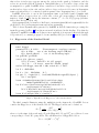
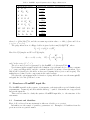
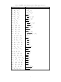
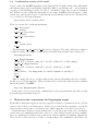
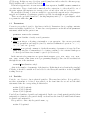
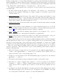
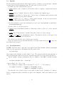
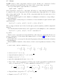
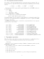
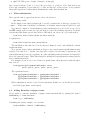
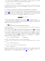
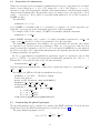
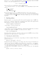
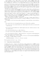
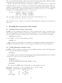
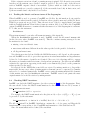
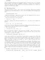
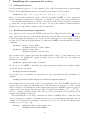
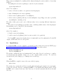
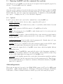
Laboratoire de Physique Théorique LAPTH
Chemin de Bellevue, B.P. 110, F-74941 Annecy-le-Vieux, Cedex, France.
Laboratory of Particle Physics, Joint Institute for Nuclear Research,
141 980 Dubna, Moscow Region, Russian Federation
arXiv:hep-ph/0208011 v1 1 Aug 2002
LAPTH-926/02
LanHEP—
a package for automatic generation
of Feynman rules in field theory
Version 2.0
A. V. Semenov
2002
LanHEP — a package for automatic generation of Feynman rules in field
theory. Version 2.0
Abstract. The LanHEP program for Feynman rules generation in momentum representation is presented. It reads the Lagrangian written in a compact form, close to the one used
in publications. It means that Lagrangian terms can be written with summation over indices
of broken symmetries and using special symbols for complicated expressions, such as covariant
derivative and strength tensor for gauge fields. The output is Feynman rules in terms of physical fields and independent parameters. This output can be written in LaTeX format and in
the form of CompHEP model files, which allows one to start calculations of processes in the
new physical model. Although this job is rather straightforward and can be done manually, it
requires careful calculations and in modern theories with many particles and vertices, such as
supersymmetric models, can lead to errors and misprints. The program allows one to introduce
into CompHEP new gauge theories as well as various anomalous terms.
E-mail: [email protected]
WWW page: http://theory.sinp.msu.ru/~semenov/lanhep.html
Introduction
LanHEP has been designed as part of the CompHEP package [1], a software for automatic
calculations in high energy physics. CompHEP allows symbolic computation of the matrix
element squared of any process with up to 6 incoming and outgoing particles for a given physical
model (i.e. a model defined by a set of Feynman rules as a table of vertices in the momentum
representation) and then numerical calculation of cross-sections and various distributions.
The main purpose of the new option given by LanHEP is to easily introduce new models.
LanHEP makes possible the generation of Feynman rules for propagators and vertices in momentum representation starting from the Lagrangian defined by a user in some simple format
very similar to canonical coordinate representation. The user should prepare a text file with
description of all Lagrangian terms in the format close to the form used in standard publications. Of course, the user has to describe all particles and parameters appearing in Lagrangian
terms.
The main LanHEP features are:
• LanHEP expands expression and combines similar terms;
• it performs the Fourier transformation by replacing derivatives with momenta of particles;
• it writes Feynman rules in the form of four tables in CompHEP format as well as tables
in LaTeX format;
• user can define the substitution rules, for example for covariant derivative;
• it is possible to define multiplets, and (if necessary) their components;
• user can write Lagrangian terms with Lorentz and multiplet indices explicitly or omit
indices (all or some of them);
• LanHEP performs explicit summation over the indices in the Lagrangian, if the corresponding components for multiplets and matrices are introduced;
• several tests can be applied to check the correctness of the Lagrangian;
• supersymmetric theories can be described using superpotential formalism;
• BRST invariance of the Lagrangian can be tested, and ghost interaction can be constructed;
• LanHEP allows the user to introduce vertices with 4 fermions or 4 colored particles (such
vertices can’t be introduced directly in CompHEP) by means of auxiliary field with constant propagator;
The LanHEP software is written in C programming language. The first version [2] was
released in August 1996.
1
1.1
Getting started with LanHEP
QED
We start with a simple exercise, illustrating the main ideas and features of LanHEP. The first
physical model is Quantum Electrodynamics.
The QED Lagrangian is
1
LQED = − Fµν F µν + ēγ µ (i∂µ + ge Aµ )e − mēe
4
3
model QED/1.
parameter ee=0.31333:’elementary electric charge’.
spinor e1/E1:(electron, mass me=0.000511).
vector A/A:(photon).
let F^mu^nu=deriv^mu*A^nu-deriv^nu*A^mu.
lterm -1/4*(F^mu^nu)**2 - 1/2*(deriv^mu*A^mu)**2.
lterm E1*(i*gamma*deriv+me)*e1.
lterm ee*E1*gamma*A*e1.
Figure 1: LanHEP input file for the generation of QED Feynman rules
and the gauge fixing term in Feynman gauge has the form
1
LGF = − (∂µ Aµ )2 .
2
Here e(x) is the spinor electron-positron field, m is the electron mass, Aµ (x) is the vector photon
field, F µν = ∂µ Aν − ∂ν Aµ , and ge is the elementary electric charge.
The LanHEP input file to generate the Feynman rules for QED is shown in Fig. 1.
First of all, the input file consists of statements. Each statement begins with one of the
reserved keywords and ends by a full-stop ’.’ symbol.
First line says that this is a model with the name QED and number 1. This information is supplied for CompHEP, the name QED will be displayed in its list of models. In CompHEP package
each model is described by four files: ’varsN.mdl’, ’funcN.mdl’, ’prtclsN.mdl’, ’lgrngnN.mdl’ ,
where N is the very number specified in the model statement.
The model statement stands first in the input file. If this statement is absent, LanHEP
does not generate the four standard CompHEP files, but just builds the model and prints a
diagnostic, if errors are found.
The second line in the input file contains declaration of the model parameter, denoting
elementary electric charge ge as ee. For each parameter used in the model one should declare
its numeric value and an optional comment (it is also used in CompHEP menus).
The next two lines declare particles. Statement names spinor, vector correspond to the
particle spin. So, we declare electron denoted by e1 (the corresponding antiparticle name is
E1) and photon denoted by A (with antiparticle name being A, since the antiparticle for photon
is identical to particle).
After the particle name we give in brackets some options. The first one is the full name of
the particle, used in CompHEP; the second option declares the mass of this particle.
The let statement in the next line declares the substitution rule for symbol F.
∂
Predefined name deriv, which is reserved for the derivative ∂x
, will be replaced after the
Fourier transformation by the momentum of the particle multiplied by −i.
The rest of the lines describe terms in the Lagrangian. Here the reserved name gamma denotes
Dirac’s γ-matrices.
One can see that the indices are written separated with the caret symbol ’ˆ’. Note that in
the last two lines we have omitted indices. It means that LanHEP restores omitted indices
automatically. Really, one can type the last term in the full format:
lterm ee*E1^a*gamma^a^b^mu*A^mu*e1^b.
µ
It corresponds to ge ēa γab
eb Aµ with all indices written. Note that the order of objects in the
monomial is important to restore indices automatically.
4
1.2
QCD
Now let us consider the case of Quantum Chromodynamics. The Lagrangian for the gluon
fields reads
1
a
,
LY M = − F aµν Fµν
4
where
a
Fµν
= ∂µ Gaν − ∂ν Gaµ − gs f abc Gbµ Gcν ,
Gaµ (x) is the gluon field, gs is the strong coupling constant and f abc are purely imaginary
structure constants of the SU(3) color group.
The quark kinetic term and its interaction with the gluon has the form
LF = q̄i γ µ ∂µ qi + gs λaij q̄i γ µ qj Gcµ ,
where λaij are Gell-Mann matrices.
Gauge fixing terms in Feynman gauge together with the corresponding Faddev-Popov ghost
term are
1
− (∂µ Gµa )2 + igs f abc c̄a Gbµ ∂ µ cc ,
2
where (c, c̄) are unphysical ghost fields.
The corresponding LanHEP input file is shown in Fig. 2.
model QCD/2.
parameter gg=1.117:’Strong coupling’.
spinor q/Q:(quark, mass mq=0.01, color c3).
vector G/G:(gluon, color c8, gauge).
let F^mu^nu^a = deriv^nu*G^mu^a - deriv^mu*G^nu^a gg*f SU3^a^b^c*G^mu^b*G^nu^c.
lterm -F**2/4-(deriv*G)**2/2.
lterm Q*(i*gamma*deriv+mq)*q.
lterm i*gg*f SU3*ccghost(G)*G*deriv*ghost(G).
lterm gg*Q*gamma*lambda*G*q.
Figure 2: Input file for the generation of QCD Feynman rules
Table 1: QCD Feynman rules generated by LanHEP in LaTeX output format
Fields in the vertex
Gµp η̄qG η G r
q̄ap
qbq
Gµr
Gµp
Gνq
Gρr
Gµp
Gνq
Gρr
Variational derivative of Lagrangian by fields
−gs pµ3 fpqr
µ r
gs γab
λpq
Gσs
gs fpqr (pν3 g µρ − pρ2 g µν − pµ3 g νρ + pρ1 g µν + pµ2 g νρ − pν1 g µρ )
gs2 (g µρ g νσ fpqt frst − g µσ g νρfpqt frst + g µν g ρσ fprt fqst
+g µν g ρσ fpst fqrt − g µσ g νρ fprt fqst − g µρ g νσ fpst fqrt )
Since QCD uses objects with color indices, one has to declare the indices of these objects.
There are three types of color indices supported by LanHEP. These types are referred as color
c3 (color triplets), color c3b (color antitriplets), and color c8 (color octets). One can see
5
that color c3 index type appears among the options in the quark q declaration, and the
color c8 one in the gluon G declaration. Antiquark Q has got color index of type color c3b
as antiparticle to quark. LanHEP allows contraction of an index of type color c3 only with
another index of type color c3b, and two indices of type color c8. Of course, in Lagrangian
terms each index has to be contracted with its partner, since Lagrangian has to be a scalar.
LanHEP allows also to use in the Lagrangian terms a predefined symbol lambda with
the three indices of types color c3, color c3b, color c8 corresponding to Gell-Mann λmatrices. Symbol f SU3 denotes the structure constant f abc of color SU(3) group (all three
indices have the type color c8).
Option gauge in the declaration of G allows to use names ghost(G) and ccghost(G) for the
ghost fields c and c̄ in Lagrangian terms and in let statements.
Table 1 shows Feynman rules generated by LanHEP in LaTeX format after processing the
input file presented in Fig. 2. Four gluon vertex rule is indicated in the last line. Note that the
output in CompHEP format has no 4-gluon vertex explicitly; it is expressed effectively through
3-leg vertices by a constant propagator of some auxiliary field (see section 9 for more details).
1.3
Higgs sector of the Standard Model
model Higgs/1.
parameter EE = 0.31333 : ’Electromagnetic coupling constant’,
SW = 0.4740 : ’sin of the Weinberg angle (PDG-94)’,
CW = Sqrt(1-SW**2) : ’cos of the Weinberg angle’.
let g=EE/SW, g1=EE/CW.
vector A/A: (photon, gauge),
Z/Z:(’Z boson’, mass MZ = 91.187, gauge),
’W+’/’W-’: (’W boson’, mass MW = MZ*CW, gauge).
scalar H/H:(Higgs, mass MH = 200, width wH = 1.461).
let B = -SW*Z+CW*A.
let W = {’W+’, CW*Z+SW*A, ’W-’}.
let phi = { -i*gsb(’W+’), (vev(2*MW/EE*SW)+H+i*gsb(Z))/Sqrt2 },
Phi = anti(phi).
lterm -2*lambda*(phi*anti(phi)-v**2/2)**2 where
lambda=(g*MH/MW)**2/16, v=2*MW*SW/EE.
let D^a^b^mu =(deriv^mu+i*g1/2*B^mu)*delta(2)^a^b
+i*g/2*taupm^a^b^c*W^mu^c,
Dc^a^b^mu=(deriv^mu-i*g1/2*B^mu)*delta(2)^a^b
-i*g/2*taupm^a^b^c*anti(W)^mu^c.
lterm D^a^b^mu*phi^b*Dc^a^c^mu*Phi^c.
Figure 3: Input file for the Higgs sector of the Standard Model
The third example illustrates using the multiplets in the framework of LanHEP. Let us
consider the Higgs sector of the Standard Model. The Higgs doublet can be defined as
Φ=
W
( 2M
ess
−iWf+
√
+ H + iZf )/ 2
!
,
where sw is the sinus of the weak angle, H is the Higgs field, Zf and Wf± are goldstone bosons
corresponding to Z and W ± gauge fields. The self-interaction of Higgs field read as
LH = −2λ(ΦΦ∗ − υ 2/2)2 ,
6
Table 2: LanHEP output: Feynman rules for Higgs self-interaction
Fields in the vertex
H H H
H
WF+
H
ZF
H
H
H
H
H
WF+
H
H
ZF
2
eM H
− 12 M
W sw
WF−
2
eM H
− 12 M
W sw
ZF
ZF
WF−
WF+
WF−
ZF
ZF
ZF
2
2
2
2
2
2
2
2
2
2
2
− 14 Me WM2H
sw 2
WF−
WF+
2
− 34 Me WM2H
sw 2
H
WF+
ZF
Variational derivative of Lagrangian by fields
eM H 2
− 32 M
W sw
WF−
− 14 Me WM2H
sw 2
− 12 Me WM2H
sw 2
− 14 Me WM2H
sw 2
ZF
− 34 Me WM2H
sw 2
ZF
where λ = (gMH /MW )2 /16, and the vaccuum expectation value υ = 2MW /g (here and below
g = e/sw , g ′ = e/cw .)
The gauge interaction of a Higgs doublet is given by the term (Dµ Φ)(D µ Φ)∗ , where
~ µ.
Dµ = ∂µ + ig ′ Bµ /2 + ig~τ W
Here B is U(1) singlet and W is SU(2) triplet,
Bµ = −sw Zµ + cw Aµ ,
Wµ+

Wµa = 
 cw Zµ + sw Aµ  ,
−
Wµ


and ~τ is the vector (τ + , τ 3 , τ − ).
The above model can be represented by the LanHEP code shown in Table 3.
New features in this example include the definition of special symbols for coupling constants
g, g ′ , gauge and Higgs fields, and the covariant derivative by means of let statement. Note
that in the declaration for the fields we have used dummy indices (vector and isospin). The
multiplets are defined by the components in the curly brackets.
Note that the option gauge in the declaration of gauge fields allows to use the name gsb(Z)
and gsb(’W+’) for the goldstone bosons.
2
Structure of LanHEP input file
The LanHEP input file is the sequence of statements, each starts with a special identifier (such
as parameter, lterm etc) and ends with the full-stop ’.’ symbol. Statement can occupy several
lines in the input file.
This section is aimed to clarify the syntax of LanHEP input files, i.e. the structure of the
statements.
2.1
Constants and identifiers
First of all, each word in any statement is either an identifier or a constant.
Indentfiers are the names of particles, parameters etc. Examples of identifiers from the
previous section are particle names
7
Table 3: LanHEP output: Feynman rules for Higgs gauge interaction
Fields in the vertex
Aµ W + ν WF−
Aµ
WF+
W −ν
Aµ
WF+
WF−
H
W +µ
W −ν
H
W +µ
WF−
H
WF+
W −µ
H
Zµ
Zν
H
Zµ
ZF
W +µ
WF−
Zν
W +µ
WF−
ZF
WF+
W −µ
Zν
WF+
W −µ
ZF
WF+
WF−
Variational derivative of Lagrangian by fields
ieMW g µν
−ieMW g µν
−e(pµ2 − pµ3 )
eMW µν
g
sw
− 12 siew (pµ1 − pµ3 )
1 ie
(pµ2 − pµ1 )
2 sw
eMW µν
g
cw 2 sw
− 12 cwiesw (pµ1 −
sw µν
g
− ieMcW
w
1 e
(pµ3 − pµ2 )
2 sw
ieMW sw µν
g
cw
1 e
(pµ1 − pµ3 )
2 sw
2
w )e
(pµ1 − pµ2 )
− 12 (1−2s
cw sw
Zµ
Aµ
Aν
WF+
WF−
Aµ
H
W +ν
WF−
Aµ
H
WF+
W −ν
Aµ
W +ν
WF−
ZF
Aµ
WF+
W −ν
ZF
Aµ
WF+
WF−
2e2 g µν
1 ie2 µν
g
2 sw
2
g µν
− 12 ie
sw
H
W +µ
H
H
Zµ
H
W +µ
WF−
Zν
H
WF+
W −µ
Zν
2
− 12 sew g µν
2
− 12 sew g µν
(1−2sw 2 )e2 µν
g
cw sw
Zν
H
1 e2 µν
g
2 sw 2
W −ν
e2
1
g µν
2 cw 2 sw 2
Zν
2
− 12 ie
g µν
cw
1 ie2 µν
g
2 cw
1 e2 µν
g
2 sw 2
W +µ
WF+
W −ν
W +µ
W −ν
ZF
W +µ
WF−
Zν
ZF
1 e2 µν
g
2 cw
WF+
W −µ
Zν
ZF
1 e2 µν
g
2 cw
WF+
WF−
Zµ
Zν
ZF
Zµ
pµ3 )
WF−
ZF
Zν
ZF
1 e2 µν
g
2 sw 2
1 (1−2sw 2 )2 e2 µν
g
2
cw 2 sw 2
1
e2
g µν
2 cw 2 sw 2
8
e1 E1 A q Q G
The first word in each statement is also an identifier, defining the function which this statement
performs. The identifiers are usually combinations of letters and digits starting with a letter.
If an identifier does not respect this rule, it should be quoted. For example, the names of W ±
bosons must be written as ’W+’ and ’W-’, since they contain ’+’ and ’–’ symbols.
Constants can be classified as
• integers: they consist of optional sign followed by one or more decimal digits, such as
0
1
-1
123
-98765
Integers can appear in Lagrangian terms, parameter definition and in other expressions.
• Floating point numbers include optional sign, several decimal digits of mantissa with an
embedded period (decimal point) with at least one digit before and after the period, and
optional exponent. The exponent, if present, consist of letter E or e followed by an optional
sign and one or more decimal digits. Valid examples of floating point numbers are
1.0
-1.0
0.000511
5.11e-4
Floating point numbers are used only as parameter values (coupling constants, particle
masses etc). They can not be explicitly used in Lagrangian terms.
• String constants may include arbitrary symbols. They are used as comments in parameter
statements, full particle names in the declaration of a particle, etc. Examples from the
previous section are
electron
photon
If a string constant contains any character besides letters and digits or does not begin with
a letter, it should be quoted. For example, the comments in QED and QCD input files
(see previous section) contain blank spaces, so they are quoted:
’elementary electric charge’
’Strong coupling’
2.2
Comments
User can include comments into the LanHEP input file in two ways. First, symbol ’%’ denotes
the comment till the end of current line. Second way allows one to comment any number of lines
by putting a part of input file between ’/*’ (begin of comment) and ’*/’ (end of comment)
symbols.
2.3
Including files
LanHEP allows the user to divide the input file into several files. To include the file file, the
user should use the statement
read file.
The standard extension ’.mdl’ of the file name may be omitted in this statement.
Another way to include a file is provided by the use statement as
use file.
The use statement reads the file only once, next appearances of this statement with the same
argument do nothing. This function prevents multiple reading of the same file. This form
can be used mainly to include some standard modules, such as declaration of Standard Model
particles to be used for writing some extensions of this model.
9
2.4
Conditional processing of the model
Let us consider the LanHEP input files for the Standard Model with both the t’Hooft-Feynman
and unitary gauges. It is clear that these input files differ by several lines only — the declaration
of gauge bosons and Higgs doublet. It is more convenient to have only one model definition
file. In this case the conditional statements are necessary. LanHEP allows the user to define
several keys, and use these keys to branch among several variants of the model. The keys have
to be declared by the keys statement:
keys name1=value1, name2=value2, ... .
Then one can use the conditional statements:
do if key==value1.
actions1
do else if key==value2.
actions2
do else if key==value3.
...
do else.
default actions
end if.
The statements do else if and do else are not obligatory. The value of the key is a number
or symbolic string. An example of using these statement in the Standard model may read:
keys Gauge=unitary.
do if Gauge==Feynman.
vector Z/Z:(’Z-boson’,mass MZ = 91.187, width wZ = 2.502, gauge).
do else if Gauge==unitary.
vector Z/Z:(’Z-boson’,mass MZ = 91.187, width wZ = 2.502).
do else.
write(’Error: key Gauge must be either Feynman or unitary’).
quit.
end if.
Thus, to change the choice of gauge fixing in the generated Feynman rules it is enough to
modify one word in the input file. There is another way, to set the key value from the command
line at the launch of LanHEP:
lhep -key Gauge=Feynman filename.
If the value of key is set from the command line at the program launch, the value for this
key in the keys statement is ignored.
3
Objects in the expressions for Lagrangian terms
Each symbol which may appear in algebraic expressions (names of parameters, fields, etc) has
a fixed order of indices and their types. If this object is used in any expression, one should
write its indices in the same order as they were defined when the object has been declared.
Besides the types of indices corresponding to the color SU(3) group: color c3 (color triplet),
color c3b (color antitriplet) and color c8 (color octet) described in the previous example,
there are default types of indices for Lorentz group: vector, spinor and cspinor (antispinor).
User can also declare new types of indices corresponding to the symmetries other than color
10
SU(3) group. In this case any object (say, particle) may have indices related to this new group.
This possibility will be described in Section 8.
If an index appears twice in some monomial of an expression, LanHEP assumes summation
over this index. Types of such indices must allow the contraction, i.e. they should be one of
the pairs: spinor and cspinor, two vector, color c3 and color c3b, two color c8.
In general the following objects are available to appear in the expressions for a Lagrangian:
integers and identifiers of parameters, particles, specials, let-substitutions and arrays.
2
There are also predefined
√ symbols i, denoting imaginary unit i (i = −1) and Sqrt2, which
is a parameter with value 2.
3.1
Parameters
Parameters are scalar objects (i.e. they have no indices). Parameters denote coupling constants,
masses and widths of particles, etc. To introduce a new parameter one should use the parameter
statement, which has the generic form
parameter name=value:comment.
• name is an identifier of newly created parameter.
• value is an integer or floating point number or an expression. One can use previously
declared parameters and integers joined by standard arithmetical operators ’+’, ’-’,
’*’, ’/’, and ’**’ (power).
• comment is an optional comment to clarify the meaning of parameter, it is used in CompHEP help windows. Comment has to be a string constant, so if it contains blank spaces
or other special characters, it must be quoted (see Section 3).
In the extression for parameters one can use functions sqrt, pow, sin, asin, cos, acos,
tan, atan, atan2, fabs (same as in C programming language). One can add new functions
through the use of the statement
external func(function, arity).
Arity is the number of arguments of the function. If this function is absent in the standard
C library, it should be written in C and added to the library file usrlib.a in the CompHEP
working directory.
3.2
Particles
Particles are objects to denote physical particles. They may have indices. It is possible to
use three statements to declare a new particle, at the same time the second and the third
statements define the corresponding Lorentz index:
scalar P/aP:(options).
spinor P/aP:(options).
vector P/aP:(options).
P and aP are identifiers of particle and antiparticle. In the case of truly neutral particles (when
antiparticle is identical to the particle itself) one should use the form P/P with identical names
for particle and antiparticle.
It is possible to write only the particle name, e.g.
scalar P:(options).
11
In this case the name of corresponding antiparticle is generated automatically. It satisfies the
usual CompHEP convention, when the name of antiparticle differs from particle by altering the
case of the first letter. So for electron name e1 automatically generated antiparticle name will
be E1. If the name contains symbol ’+’ it is replaced by ’–’ and vice versa.
The option is comma-separated list of options for a declared particle, and it may include the
following items:
• the first element in this list must be the full name of the particle, (e.g. electron and
photon in our example.) Full name is a string constant, so it should be quoted if it
contains blanks, etc.
• mass param=value defines the mass of the particle. Here param is an identifier of a new
parameter, which is used to denote the mass; value is its value, it has the same syntax as in
the parameter statement, comment for this new parameter being generated automatically.
If this option omitted, the mass is assumed to be zero.
• width param=value declares the width of the particle. It has the same syntax as for mass
option.
• itype is a type of index of some symmetry; one can use default index types for color SU(3)
group (see QCD example in Section 2). It is possible to use user-defined index types (see
Section 8) and Lorentz group indices vector, spinor, cspinor.
• left or right says that the massless spinor particle is an eigenstate of (1 − γ 5 )/2 or
(1 + γ 5 )/2 projectors, so this fermion is left-handed or right-handed.
• gauge declares the vector particle as a gauge boson. This option generates the corresponding ghosts and goldstone bosons names for the named particle (see below).
When a particle name is used in any expression (in Lagrangian terms), one should remember
that the first index is either a vector or a spinor (if this particle is not a Lorentz scalar). Then
the indices follow in the same order as index types in the options list. So, in the case of quark
declaration (see the QCD example) the first index is spinor, and the second one is color triplet.
There are several functions taking particle name as an argument which can be used in
algebraic expressions. These functions are replaced with auxiliary particle names, which are
generated automatically.
• Ghost field names in gauge theories are generated by the functions ghost(name) →
’name.c’ and ccghost(name) → ’name.C’ (see for instance Table 1). Here and below
name is the name of the corresponding gauge boson.
• Goldstone boson field name in the t’Hooft-Feynman gauge is generated by the function
gsb(name) → ’name.f’.
• The function anti(name) generates antiparticle name for the particle name.
• The name for a charge conjugate spinor particle ψ c = C ψ̄ T is generated by the function
cc(name) → ’name.c’. Charge conjugate fermion has the same indices types and ordering, however index of spinor type is replaced by the index type cspinor and vice
versa.
• vev(expr) is used in the Lagrangian for vacuum expectation values. Function vev ensures
that deriv*vev(expr) is zero. In other words, vev function forces LanHEP to treat expr
as a scalar particle which will be replaced by expr in Feynman rules.
12
3.3
Specials
Besides parameters and particles other indexed such as γ-matrices, group structure constants,
etc may appear in the Lagrangian terms. We refer such objects as specials.
Predefined specials of the Lorentz group are:
• gamma stands for the γ µ -matrices. It has three indices of spinor, cspinor and vector
types.
• gamma5 denotes γ 5 matrix. It has two indices of spinor and cspinor types.
• moment has one index of vector type. At the stage of Feynman rules generation this
symbol is replaced by the particle moment.
• deriv is replaced by −ipµ , where pµ is the particle moment. It has one vector index.
Note that deriv*A*B means (∂A)B, not ∂(AB).
• For the derivative of a product, derivp(expr) can be used. derivp(A*B) is equivalent to
deriv*A*B+A*deriv*B.
Specials of the color SU(3) group are:
• lambda denotes Gell-Mann λ-matrices. It has three indices: color c3, color c3b and
color c8.
• f SU3 is the SU(3) structure constant. It has three indices of color c8 type.
• eps c3 and eps c3b are antisymmetric tensors. The first has 3 indices of the type color
c3, and the second 3 color c3b indices.
Note that for specials the order of indices types is fixed.
Users can declare new specials with the help of a facility defined in Section 8 to introduce
user-defined indices types.
3.4
Let-substitutions
LanHEP allows the user to introduce new symbols and then substitute them in Lagrangian
terms by some expressions. Substitution has the generic form
let name=expr.
where name is the identifier of newly defined object. The expression has the same structure as
those in Lagrangian terms, however here expression may have free (non-contracted) indices.
Typical example of using a substitution rule is a definition of the QED covariant derivative
as
let Deriv^mu=deriv^mu + i*ee*A^mu.
corresponding to Dµ = ∂µ + ige Aµ .
More complicated example is the declaration σ µν ≡ i(γ µ γ ν − γ ν γ µ )/2 matrices:
let sigma^a^b^mu^nu = i*(gamma^a^c^mu*gamma^c^b^nu
- gamma^a^c^nu*gamma^c^b^mu)/2.
Note that the order of indices types of new symbol is fixed by the declaration. So, first two
indices of sigma after this declaration are spinor and antispinor, third and fourth are vector
indices.
13
3.5
Arrays
LanHEP allows to define components of indexed objects. In this case, contraction of indices
will be performed as an explicit sum of products of the corresponding components.
An object with explicit components has to be written as
{expr1, expr2 ..., exprN }^i
where expressions correspond to components. All indices of components (if present) have to
be written at the each component, and the index numbering components has to be written
after closing curly bracket. Of course, all the components must have the same types of free
(non-contracted) indices.
Arrays are usually applied for the definition of multiplets and matrices corresponding to
broken symmetries.
Typical example of arrays usage is a declaration of electron-neutrino isospin doublet l1 (and
antidoublet L1)
let l1^a^I = { n1^a, e1^a}^I, L1^a^I = { N1^a, E1^a}^I.
Here we suppose that n1 was declared as the spinor particle (neutrino), with the antiparticle
name N1.
Note that the functions anti and cc can be applied also to the multiplets, so the construction
let l1^a^I = { n1^a, e1^a}^I, L1^a^I = anti(l1)^a^I.
is possible.
Matrices can be represented as arrays which have other arrays as components. However, it
is more convenient to declare them with dummy indices, see Section 5.4 (the same is correct
for multiplets also).
It is possible also to use arrays directly in the Lagrangian, rather than only in the declaration
of let-substitution.
When LanHEP is launched, it has already declared some frequently used matrices. They
are:
• tau1, tau2, tau3 are τ -matrices τ1 , τ2 , τ3 :
τ1 =
0 1
1 0
!
,
τ2 =
0 −i
i 0
!
,
τ3 =
1
0
0 −1
!
;
• tau is a vector ~τ = (τ1 , τ2 , τ3 );
√
• taup and taum are matrices τ ± = (τ 1 ± iτ 2 )/ 2;
• taupm is a vector (τ + , τ 3 , τ − );
• eps is the antisymmetrical tensor ε (ε123 = 1);
• Tau1, Tau2, Tau3 are generators of SU(2) group adjoint representation (3-dimensional
analog of τ -matrices) T 1 , T 2 , T 3 with commutative relations [Ti , Tj ] = −iǫijk Tk :


0 −1 0
1 
0 1 
T 1 = √  −1
,
2
0
1 0


0 i 0
1 

T 2 = √  −i 0 −i  ,
2
0 i 0
√
• Taup and Taum corresponds to T ± = (T 1 ± iT 2 )/ 2;
• Taupm is a vector T~ = (T + , T 3, T − ).
14


1 0
0

0 
T3 =  0 0
;
0 0 −1
3.6
Two-component notation for fermions
It is possible to write the Lagrangian using two-component notation for fermions. The connection between two-component and four-component notations is summarized by the following
relations:
!T
!T
!
!
ξ
η
η
ξ
c
c
.
,
ψ̄ =
ψ̄ = ¯
,
ψ = ¯ ,
ψ=
η̄
ξ
ξ
η̄
If the user has declared a spinor particle p (with antiparticle P), the LanHEP notation for
its components is:
ξ → up(p)
η̄ → down(p)
η → up(cc(p)) or up(P)
ξ¯ → down(cc(p)) or down(P)
To use the four-vector σ̄ µ one should use the statement
special sigma:(spinor2,spinor2,vector).
Note that the sigma object is not defined by default, thus the above statement is required. It is
possible also to use another name instead of sigma (this object can be recognized by LanHEP
by the types of its indices).
LanHEP uses the following rules to convert the two-component fermions to four-component
ones (we use PR,L = (1 ± γ 5 )/2):
η1 ξ2 = ψ̄1 PL ψ2
η̄1 ξ¯2 = ψ̄1 PR ψ2
ξ1 ξ2 = ψ̄1c PL ψ2
ξ¯1 ξ¯2 = ψ̄1 PR ψ2c
ξ1 η2 = ψ̄1c PL ψ2c
ξ¯1 η̄2 = ψ̄1c PR ψ2c
η1 η2 = ψ̄1 PL ψ2c
η̄1 η̄2 = ψ̄1c PR ψ2
ξ¯1 σ µ ξ2 = ψ̄1 γ µ PL ψ2
η̄1 σ µ η2 = ψ̄1c γ µ PL ψ2c
4
up(P1)*up(p2)
down(P1)*down(p2)
up(p1)*up(p2)
down(P1)*down(P2)
up(p1)*up(P2)
down(p1)*down(P2)
up(P1)*up(P2)
down(p1)*down(p2)
down(P1)*sigma*up(p2)
down(p1)*sigma*up(P2)
→
→
→
→
→
→
→
→
P1*(1-gamma5)/2*p2
P1*(1+gamma5)/2*p2
cc(p1)*(1-gamma5)/2*p2
P1*(1+gamma5)/2*cc(P2)
cc(p1)*(1-gamma5)/2*cc(P2)
cc(p1)*(1+gamma5)/2*cc(P2)
P1*(1-gamma5)/2*cc(P2)
cc(p1)*(1+gamma5)/2*p2
→ P1*gamma*(1-gamma5)/2*p2
→ cc(p1)*gamma*(1-gamma5)/2*cc(P2)
Lagrangian expressions
When all parameters and particles necessary for the introduction of a (physical) model are
declared, one can enter Lagrangian terms with the help of the lterm statement:
lterm expr.
Elementary objects of expression are integers, identifiers of parameters, particles, specials,
let-substitutions, and arrays.
These elementary objects can be combined by the usual arithmetic operators as
• expr1+expr2 (addition),
• expr1–expr2 (subtraction),
• expr1*expr2 (product),
• expr1/expr2 (fraction; here expr2 must be a product of integers and parameters),
15
• expr1**N (Nth power of expr1; N must be an integer).
One can use brackets ’(’ and ’)’ to force the precedence of operators. Note, that indices can
follow only elementary objects symbols, i.e. if A1 and A2 were declared as two vector particles
then valid expression for their sum is A1^mu+A2^mu, rather than (A1+A2)^mu.
4.1
Where-substitutions
More general form of expressions involves where-substitutions:
expr where subst.
In the simple form subst is name=repl or several constructions of this type separated by
comma ’,’. In the form of such kind each instance of identifier name in expr is replaced by repl.
Note that in contrast to let-substitutions, where-substitution does not create a new object.
LanHEP simply replaces name by repl, and then processes the resulting expression. It means
in particular that name can not have indices, although it can denote an object with indices:
lterm F**2 where F=deriv^mu*A^nu-deriv^nu*A^mu.
is equivalent to
lterm (deriv^mu*A^nu-deriv^nu*A^mu)**2.
The substitution rule introduced by the keyword where is active only within the current
lterm statement.
More general form of where-substitution allows to use several name=repl substitution rules
separated by semicolon ’;’. In this case expr will be replaced by the sum of expressions; each
term in this sum is produced by applying one of the substitution rules from semicolon-separated
list to the expression expr. This form is useful for writing the Lagrangian where many particles
have a similar interaction.
For example, if u,d,s,c,b,t are declared as quark names, their interaction with the gluon
may read as
lterm gg*anti(psi)*gamma*lambda*G*psi where
psi=u; psi=d; psi=s; psi=c; psi=b; psi=t.
The equivalent form is
lterm gg*U*gamma*lambda*G*u + gg*D*gamma*lambda*G*d +
gg*C*gamma*lambda*G*c + gg*S*gamma*lambda*G*s +
gg*T*gamma*lambda*G*t + gg*B*gamma*lambda*G*b.
Where-substitution can also be used in let statement. In this case one should use brackets:
let lsub=(expr where wsub=expr1).
4.2
Adding Hermitian conjugate terms
It is possible to generate hermitian conjugate terms automatically by putting the symbol
AddHermConj to lterm statement:
lterm expr + AddHermConj.
Continuing the former example, one can write:
lterm a*H*H*h + b*H**3 + AddHermConj.
16
Note, that the symbol AddHermConj adds the hermitian conjugate expressions to all terms
in the lterm statement. It means in particular that in the statement
lterm expr1 + (expr2 + AddHermConj).
the conjugate terms are added to both expr1 and expr2 . Thus, one should not place selfconjugate terms in the lterm statement where AddHermConj present (or one should supply
these terms with 1/2 factor).
4.3
Using the superpotential formalism in the MSSM and its extensions
In supersymmetric models (in particular, in the Minimal Supersymmetric Standard Model
(MSSM) [3]) one makes use of the superpotential — a polynomial W depending on scalar fields
Ai (superpotential also can be defined in terms of superfields, we do not consider this case).
Then, there is the contribution to the Lagrangian: Yukawa terms in the form
1
−
2
∂2W
Ψi Ψj + H.c.
∂Ai ∂Aj
!
and Fi∗ Fi terms, where Fi = ∂W/∂Ai (for more details, see [3] and references therein).
To use this formalism in LanHEP, one should define first the multiplets of matter fields
and then define the superpotential through the let-substitution statement. The example of the
MSSM with a single generation may read:
keep lets W.
let W=eps*(mu*H1*H2+ml*H1*L*R+md*H1*Q*D+mu*H2*Q*U).
Here symbols H1, H2, L, R, Q, U, D are defined somewhere else as doublets and singlets in
terms of scalar particles.
Note that before the definition of W this symbol should appear in the keep lets statement.
It is necessary to notify LanHEP that let-substitutions (multiplets) at the definition of W should
not be expanded. Without this statement, the representation used by LanHEP for W will not
contain symbols of multiplets but only the particles which were used at multiplets definition.
Since W was declared in the keep lets statement and contains the symbols of multiplets,
one can evaluate the variational derivative of W by one or two multiplets, e.g. df(W,H1) or
df(W,H1,L). Thus the Yukawa terms may be written:
lterm - df(W,H1,H2)*fH1*fH2 - ...
+ AddHermConj.
Here fH1, fH2 are fermionic partners of corresponding multiplets.
To introduce the Fi∗ Fi terms one needs to declare the conjugate superpotential, e.g. Wc, and
write:
lterm - df(W,H1)*df(Wc,H1c) - ....
A better way is to use the function dfdfc(W,H1) instead:
lterm - dfdfc(W,H1) - ....
The function evaluates the variational derivative, multiply it by the conjugate expression and
returns the result. Moreover, it can introduce auxiliary fields to split vertices with 4 color
particles (in the case of CompHEP output); see Section 9 for more details.
17
4.4
Generation of counterterms
Ultraviolet divergencies in renormalized quantum field theories are compensated by renormalization of wave functions φi → φi (1 + δzi ), masses Mi → Mi + δMi , charges ei → ei + δei ,
and may be some other Lagrangian constants. Such transformation of the Lagrangian assumes
changes in the Feynman rules. In particular vertices are changed due to the appearence of new
terms — counterterms. It is possible to treat this transformation at 1-loop level by means of
LanHEP package.
The statement
transform obj -> expr.
forces LanHEP to substitute symbol of a parameter or a particle, obj, by the expression expr
when this object appears in the Lagrangian expressions of the Lagrangian.
For example, if the electric charge e in QED is renormalized than the statement
transform e -> e+d e.
makes LanHEP substitute each occurence of e symbol in further expressions by e+d e. Of
course, e and d e should be declared as parameters before this statement.
The transform statement is very similar to the let statement and uses the same syntax
for expression expr. It has however two advantages. First, one does not need to introduce new
name for transformed parameter or field. Second, if one has the LanHEP file for some physical
model, it is enough to add counterterms statements into the input file just after the statements
declaring parameters and particles.
In 1-loop approximation renormalization parameters appear in expressions only at first
power, i.e. δZi δZj = 0, where δZi means all renormalization parameters (δei , δMi , δzi , ...).
This should be done with the help of the following statement
infinitesimal d Z1, d Z2, ..., d Zn.
It declares that a monomial should be omitted if it contains more than one of parameters d Z1,
d Z2, ..., d Zn.
An example for QED model with renormalization reads as:
parameter e = 0.3133: ’Electric charge’.
vector A/A:photon.
spinor e1/E1:(electron, mass me=0.000511).
parameter d e, d me, d e1, d A.
infinitesimal d e, d me, d e1, d A.
transform e -> e*(1+d e), me -> me+d me,
A -> A*(1+d A),
e1 -> e1 + d e1*e1,
E1 -> E1 + d e1*E1.
lterm e*E1*(i*gamma*deriv+gamma*A+me)*e1.
4.5
Constructing the ghost Lagrangian
The ghost Lagrangian can be constructed by means of the BRST formalism. To use it, the user
should first declare the BRST transformations for fields (see Section 6.4).
The gauge-fixing Lagrangian reads as:
1
1
LGF = G− G+ + |GZ |2 + |Gγ |2 ,
2
2
18
where Gi (i = ±, γ, Z) are gauge-fixing functions. The ghost Lagrangian ensures the BRST
invariance of the entire Lagrangian and can be written as ([7])
LGh = −c̄i δBRST Gi + δBRST L̃Gh .
where δBRST L̃Gh is an overall function, which is BRST-invariant.
So, for the photon and Gγ = (∂ · A), the LanHEP code for gauge-fixing and ghost terms
reads as:
let G A = deriv*A.
lterm -G A**2/2.
lterm -’A.C’*brst(G A).
Here the brst function is used to get BRST-transformation of the specified expression.
The inverse BRST transformation can also be used. One can declare the transformations
for the fields by means of brsti transform. The function brsti(expr) can be used in lterm
statements.
5
Omitting indices
Physicists usually do not write all possible indices in the Lagrangian terms. LanHEP also
allows a user to omit indices. This feature can simplify the introduction of the expressions and
makes them more readable. Compare two possible forms:
lterm E1^a*gamma^a^b^mu*A^mu*e1^b.
µ
corresponding to ge ēa (x)γab
eb (x)Aµ (x), and
lterm E1*gamma^mu*e1*A^mu.
corresponding to ge ē(x)γ µ e(x)Aµ (x)). Furthermore, while physicists usually write vector indices
explicitly in the formulas, in LanHEP vector indices also can be omitted:
lterm -i*ee*E1*gamma*e1*A.
Generally speaking, when the user omits indices in the expressions, LanHEP faces two problems:
which indices were omitted and how to contract indices.
5.1
Restoring the omitted indices
When the indexed object is declared the corresponding set of indices is assumed. Thus, if the
quark q is declared as
spinor q:(’some quark’, color c3).
its first index is spinor and the second one belongs to the color c3 type. If both indices are
omitted in some expression, LanHEP generates them in the correspondence to order (spinor,
color c3). However, if only one index is written, for example in the form q^a, LanHEP has
to recognize whether the index a is of color c3 or of spinor types.
To solve this problem LanHEP looks up the list of indices omitting order. By default this
list is set to
[spinor, color c3, color c8, vector]
19
The algorithm to restore omitted indices is the following. First, LanHEP assumes that
user has omitted indices which belong to the first type (and corresponding antitype) from this
list. Continuing the consideration of our example with particle q one can see that since this
particle is declared having one spinor index (the first type in the list) LanHEP checks whether
the number of indices declared for this object without spinor index equals the number of
indices written explicitly by user. In our example (when user has written q^a) this is true. In
the following LanHEP concludes that the user omitted the spinor index and that explicitly
written index is of color c3 type.
In other cases, when the supposition fails if the user has omitted indices of the first type in
the list of indices omitting order, LanHEP goes to the second step. It assumes that user has
omitted indices of first two types from this list. If this assumption also fails, LanHEP assumes
that the user has omitted indices of first three types in the list and so on. At each step LanHEP
subtracts the number of indices of these types assumed to be omitted from the full number of
indices declared for the object, and checks whether this number of resting indices equals the
number of explicitly written indices. If LanHEP fails when the list of indices omitting order is
completed, error message is returned by the program.
Note that if the user would like to omit indices of some type, he must omit all indices of
this type (and antitype) as well as the indices of all types which precede in the list of indices
omitting order.
For example, if object Y is declared with one spinor, two vector and three color c8 indices,
than
• the form Y^a^b^c^d^e^f means that the user wrote all the indices explicitly;
• the form Y^a^b^c^d^e means that the user omitted spinor index and wrote vector and
color c8 ones;
• the form Y^a^b means that the user omitted spinor and color c8 indices and wrote only
two vector ones;
• the form Y means that the user omitted all indices;
• all other forms, involving different number of written indices, are incorrect.
One can say that indices should be omitted in the direct correspondence with abrupting the
list of indices omitting order from left to right.
One could change the list of indices omitting order types by the statement SetDefIndex.
For example, for default setting it looks like
SetDefIndex(spinor, color c3, color c8, vector).
Each argument in the list is a type of index.
5.2
Contraction of restored indices
A dummy index can be contracted only with some another dummy index. LanHEP expands
the expression and restores indices in each monomial. LanHEP reads objects in the monomial
from the left to the right and checks whether the restored indices are present. If such index
appears LanHEP seeks for the restored index of the appropriate type at the next objects.
Note, that the program does not check whether the object with the first restored index has
another restored index of the appropriate type. Thus, if F is declared as let-substitution for the
strength tensor of electromagnetic field (with two vector indices) then expression F*F (as well
as F**2) after processing dummy indices turns to the implied form F^mu^nu*F^mu^nu rather
than F^mu^mu*F^nu^nu.
20
This algorithm makes the contractions to be sensitive to the order of objects in the monomial.
Let us look again at the QED example. Expression E1*gamma*A*e1 (as well as A*e1*gamma*E1)
leads to correct result where the vector index of photon is contracted with the same index of
γ-matrix, spinor index of electron is contracted with antispinor index of γ-matrix and antispinor index of positron is contracted with spinor index of γ-matrix. However the expression
E1*e1*A*gamma leads to the wrong form E1^a*e1^a*A^mu*gamma^b^c^mu, because the first
antispinor index after the electron belongs to positron. Spinor indices of gamma stay free (noncontracted) since no more objects with appropriate indices (so, LanHEP will report an error
since Lagrangian term is not a scalar).
Note, that in the vertex with two γ-matrices the situation is more ambiguous. Let’s look at
the term corresponding to the electron anomalous magnetic moment ē(x)(γ µ γ ν − γ ν γ µ )e(x)Fµν .
The correct LanHEP expression is
e1*(gamma^mu*gamma^nu - gamma^nu*gamma^mu)*E1*F^mu^nu
Here vector indices can’t be omitted, since it lead to the contraction of vector indices of γmatrices. One can see also that the form
e1*E1*(gamma^mu*gamma^nu - gamma^nu*gamma^mu)*F^mu^nu
will correspond to the expression ē(x)e(x)Sp(γ µ γ ν )Fµν . Here LanHEP has got scalar Lorentzinvariant expression in the Lagrangian term, so it has no reason to report an error.
These examples mean that the user should clearly realize how the indices will be restored
and contracted, or (s)he has to write all indices explicitly.
5.3
Let-substitutions
Another problem arises when the dummy indices stay free, this is the case for the let statement. LanHEP allows only two ways to avoid ambiguity in the order of indices types: either
user specifies all the indices at the name of new symbol and free indices in the corresponding
expression, or he should omit all free indices.
In the latter case the order of indices types is defined following the order of free dummy
indices in the first monomial of the expression. For example if A1 and A2 are vectors and c1
and c2 are spinors, the statement
let d=A1*c1+c2*A2.
declares a new object d with two indices, the first is a vector index and the second is a spinor index according to their order in the monomial A1*c1. Of course, each monomial in the expression
must have the same types of free indices.
5.4
Arrays
The usage of arrays with dummy indices allows us to define matrices conveniently. For example,
the declaration of τ -matrices (defined in Section 3.5) can be written as
let tau1 = {{0, 1}, { 1, 0}}.
let tau2 = {{0, i}, {-i, 0}}.
let tau3 = {{1, 0}, { 0,-1}}.
One can see that in such way of declaration a matrix is written ”column by column”.
The declaration of objects with three ‘explicit’ indices can be done using the objects already
defined. For example, when τ -matrices are defined as before, it is easy to define the vector
~τ ≡ (τ1 , τ2 , τ3 ) as
let tau = {tau1, tau2, tau3}.
21
The object tau has three indices, first pair selects the element of the matrix, while the matrix
itself is selected by the third index, i.e. tau^i^j^a corresponds to τija .
On the other hand, the declaration of structure constants of a group is more complicated.
Declaring such an object one should bear in mind that omitting indices implies that in a
sequence of components the second index of an object is changed after the full cycle of the first
index, the third index is changed after the full cycle of the second one, etc. For example, a
declaration of the antisymmetrical tensor εabc can read as
let eps = {{{0,0,0}, {0,0,-1}, {0,1,0}},
{{0,0,1}, {0,0,0}, {-1,0,0}},
{{0,-1,0}, {1,0,0}, {0,0,0}}}.
One can easily see that the components are listed here in the following order:
ε111 , ε211 , ε311 , ε121 , ε221 , ε321 , ε131 , ... ε233 , ε333 .
The declaration of more complex objects such as SU(3) structure constants can be made in the
same way.
6
Checking the correctness of the model
6.1
Checking electric charge conservation
LanHEP can check whether the introduced vertices satisfy electric charge conservation law.
This option is available, if the user declares some parameter to denote elementary electric charge
(say, ee in QED example), and than indicate, which particle is a photon by the statement
SetEM(photon, param).
So, in example of Section 1 this statement could be
SetEM(A,ee).
Electric charge of each particle is determined by analyzing its interaction with the photon.
LanHEP checks whether the sum of electric charges of particles in each vertex equals zero.
6.2
Testing Hermitian conjugate terms
LanHEP is able to check the correctness of the hermitian conjugate terms in the Lagrangian.
To do this, user should use the statement:
CheckHerm.
For example, let us consider the following (physically meaningless) input file, where a charged
scalar field is declared and cubic terms are introduced:
scalar h/H.
parameter a,b,c.
lterm a*(h*h*H+H*H*h)+b*h*h*H+c*H*H*h + h**3.
CheckHerm.
The output of LanHEP is the following (here 2 is the symmetry factor):
CheckHerm: vertex (h, h, h): conjugate (H, H, H) not found.
CheckHerm: inconsistent conjugate vertices:
(H, h, h)
(H, H, h)
2*a
<->
2*a
2*b
<->
(not found)
(not found)
<->
2*c
22
If the conjugate vertex is not found, a warning message is printed. If both vertices are present
but they are inconsistent, more detailed output is provided. For each couple of the incorrect
vertices LanHEP outputs 3 kinds of monomials: 1) those which are found in both vertices
(these monomials are correctly conjugated), 2) the monomials found only in first vertex, and
3) the monomials found only in the second vertex.
6.3
Probing the kinetic and mass terms of the Lagrangian
When LanHEP is used to generate CompHEP model files, the information about particles
propagators is taken from the particle declaration, where particle mass and width (for BreitWigner’s propagators) are provided. Thus, the user is not obliged to supply kinetic and mass
terms in lterm statements. Even if these terms are written, they do not affect the CompHEP
output. LanHEP allows user to examine whether the mass sector of the Lagrangian is consistent.
To do this, use the statement
CheckMasses.
This statement must be put after all lterm statements of the input file.
When the CheckMasses statement is used, LanHEP creates the file named masses.chk
(in the directory where LanHEP was started). This file contains warning messages if some
inconsistencies are found:
• missing or incorrect kinetic term;
• mass terms with mass different from the value specified at the particle declaration;
• off-diagonal mass terms.
Note that in more involved models like the MSSM the masses could depend on other parameters and LanHEP is not able to prove that expressions in actual mass matrix and in parameters
declared to be the masses of particles are identical. Moreover, it is often impossible to express
the masses as formulas written in terms of independent parameters. For this reason LanHEP
evaluates the expressions appearing in the mass sector numerically (based on the parameter
values specified by the user).
It is typical for the MSSM that some fields are rotated by unitary matrices to diagonalize
mass terms. In some cases, values of mixing matrices elements can not be expressed by formulas
and need to be evaluated numerically. LanHEP can recognize the mixing matrix if the elements
of this matrix were used in OrthMatrix statement. LanHEP restores and prints the mass
original matrix before fields rotation by mixing matrix.
6.4
Checking BRST invariance
LanHEP can check the BRST invariance (see the reviews in [5, 6]) of the Lagrangian. First,
the user should declare the BRST transformations for the fields in the model by means of
brst transform statement:
brst transform field -> expression.
For example, the BRST transformation for the photon δAµ = ∂µ cA + ie(Wµ+ c− − Wµ− c+ ) can
be prescribed by the statement:
brst transform A -> deriv*’A.c’+i*EE*(’W+’*’W-.c’-’W-’*’W+.c’).
The file ’sm brst.mdl’ in LanHEP distribution contains the code for gauge and Higgs fields
transformation corresponding to the CompHEP implementation of the Standard model.
Since the transformations are defined, the statement
23
CheckBRST.
enables the BRST transformation for Lagrangian terms (so it should be placed before the first
lterm statement). The output is CompHEP or LaTeX file. Certainly, if the Lagrangian is
correct, the output files are empty. However some expressions identical to zero could be not
simplified and remain in the output.
6.5
Extracting vertices
New statement allows to extract a class of vertices into separate file. This feature is useful in
checking large models with thousands of vertices, such as the MSSM. The statement has the
form
SelectVertices(file, vlist ).
Here file is a file name to output selected vertices, and vlist determines the class of vertices.
The pattern vlist may have two possible formats.
In the first format vlist is a list of particles:
[P1, P2, P3, ... Pn ]
All vertices consisting only of the listed particles P1, P2,... are extracted. For example, the
pattern
[A, Z, ’W+’, ’W-’, e1, E1, n1, N1]
selects vertices of leptons of first generation interaction with gauge fields and the self-interaction
of gauge fields (we used here particles notation of CompHEP).
The second format reads
[P11/P12../P1n, P21/.../P2m, ... ]
Here are several groups of particles, each group is joined by slash ’/’ symbol. Selected vertices
have the number of legs equal to the number of groups in the list, each leg in the vertex
corresponds to one group. For example,
[e1/E1/n1/N1, e1/E1/n1/N1, A/Z/’W+’/’W-’]
selects vertices with two legs corresponding to leptons, third leg is gauge boson. Thus, this
pattern extracts vertices of leptons interactions with gauge bosons. Note that the vertices of
gauge bosons interaction are not selected in this case. If a group consists of one particle, it
must be typed twice to enable second format (e.g. [P1/P1, P2/P2, P3/P3] for the vertex
consisting of particles P1, P2, P3.
It is possible to specify some options in SelectVertices statement. The WithAnti option
adds antiparticle names for each particle in the list (in the first format) or in the each group (in
the second format. The Delete option removes selected vertices from the LanHEP’s internal
vertices list, so these vertices are not written in output file lgrngN.mdl (lgrngN.tex). This
could be useful if SelectVertices statements are supposed to distribute all vertices which
should be in the model, than some ’unexpected’ vertices can be found in output lgrngN.mdl
file.
An example of lepton-gauge vertices selection could read as
SelectVertices( ’lept-gauge.mdl’, [e1/n1, e1/n1, A/Z/’W+’], WithAnti, Delete).
24
7
7.1
Simplifying the expression for vertices
Orthogonal matrices
If some parameters appear to be the elements of the orthogonal matrix such as quark mixing
Cabbibo-Kobayashi-Maskava matrix, one should declare them by the statement
OrthMatrix( {{a11 , a12 , a13 }, {a21 , a22 , a23 }, {a31 , a32 , a33 }} ).
where aij denote the parameters. Such a declaration permits LanHEP to reduce expressions
which contain these parameters by taking into account the properties of the orthogonal matrices.
Note that this statement has no relation to the arrays; it just declares that these parameters
aij satisfy the correspondent relations. Of course, one can declare further a matrix with these
parameters as components by means of the let statement.
7.2
Reducing trigonometric expressions
Some physical models, such as the MSSM and general Two Higgs Doublet Model [4], involve
large expressions built up of trigonometric functions. In particlular, after the diagonalization
of the Lagrangian in the Higgs sector, in the models mentioned above two angles, α and β,
are introduced, thus the Lagrangian may be written in LanHEP notation using the following
definitions:
parameter sa=0.5:’sinus alpha’,
ca=Sqrt(1-sa**2):’cosine alpha’.
parameter sb=0.9:’sinus beta’,
cb=Sqrt(1-sb**2):’cosine beta’.
One can find in the output expressions like sa*cb+ca*sb = sin(α + β) and much more complicated ones. To simplify the output and make it more readable the user can define new
parameters, for example:
parameter sapb=sa*cb+ca*sb:’sin(a+b)’.
In order to force LanHEP to substitute the expression sa*cb+ca*sb by the parameter sapb,
one should use the statement
SetAngle(sa*cb+ca*sb=sapb).
It is possible also to substitute an expressions by any polynomial involving paramters, for
example,
SetAngle((sa*cb+ca*sb)**2+(sa*cb-ca*sb)**2=sapb**2+samb**2).
where samb should be previously declared as a parameter. Note, that LanHEP expands both
expressions before setting the substitution rule. The left-hand side expression can also contain
symbols defined by let statement. In the Lagrangian expressions LanHEP expresses powers of
cosines, ca**N and cb**N through sines using recursively the formula cosN α = cosN −2 (1 −
sin2 α) to combine all similar terms. The same procedure is performed for the left-hand side
expression in SetAngle statement.
If the substitution for one angle combination is defined, LanHEP offers to define the other
ones for expressions consisting of parameters used in previous SetAngle statements. In our
example, for all expressions consisting of parameters ca, cb, sa, sb, the following message
is printed (e.g. for cos(α + β)):
Warning:
undefined angle combination; use:
SetAngle(ca*cb-sa*sb=aa000).
25
Here aa000 is an automatically generated parameter. The message is printed only once for
each expression. This feature is disabled by default; to enable producing these messages, one
should issue the statement
option UndefAngleComb=1.
7.3
Heuristics for trigonometric expressions
LanHEP can apply several heuristic algorithms to simplify these expressions. For each angle
α, the user should declare parameters for sin α, cos α, sin 2α, cos 2α, tan α. Than one should
use the angle statement:
angle sin=p1, cos=p2, sin2=p3, cos2=p4, tan=p5, texname=name.
Here pN — parameter identifiers, name — LaTeX name for angle, it is used to generate automatically LaTeX names for trigonometric functions of this angle if these names are not set
explicitly by SetTexName statement. This statement should immediately follow the declaration
of the parameters for sin α and cos α. Only the sin and cos options are obligatory. Other
parameters (i.e. sin 2α, cos 2α, tan α) should be declared if these parameters are defined before
sin α and cos α. If the former parameters will be declared in terms of latter ones, they are
recognized automatically and they need not appear in angle statements.
For example, the declaration for trigonometric functions of β angle in MSSM may read:
parameter tb=2.52:’Tangent beta’.
parameter sb=tb/Sqrt(1+tb**2):’Sinus beta’.
parameter cb=Sqrt(1-sb**2):’Cosine beta’.
angle sin=sb, cos=cb, tan=tb, texname=’\\beta’.
parameter s2b=2*sb*cb:’Sinus 2 beta’.
parameter c2b=cb**2-sb**2:’Cosine 2 beta’.
Here the parameters s2b and c2b are recognized automatically by LanHEP as sin 2α and cos 2α
since they are declared in terms of sa, ca parameters.
For a couple of angles ( α, β in this example) the user should declare the parameters for
sin(α + β), cos(α + β), sin(α − β), and cos(α − β) to allow using all implemented heuristics:
parameter
parameter
parameter
parameter
sapb=sa*cb+ca*sb
samb=sa*cb-ca*sb
capb=ca*cb-sa*sb
camb=ca*cb+sa*sb
:
:
:
:
’sin(a+b)’.
’sin(a-b)’.
’cos(a+b)’.
’cos(a-b)’.
These parameters are recognized as trigonometric functions automatically, by analysis of the
right-side expressions.
It is possible to control the usage of heuristics by the statement:
option SmartAngleComb=N.
where N is a number:
0 heuristics are switched off;
1 heuristics are switched on (by default);
2 same as 1, prints the generated substitution rule if the simplified expressions consists of
more than 3 monomials;
3 same as 1, prints all generated substitution rule.
26
4 same as 1, prints all generated substitution rule and some intermediate expressions (debug
mode).
The substitution rules are printed as SetAngle statement and can be used for manual improvement of expressions.
7.4
LaTeX output
LanHEP generates LaTeX output instead of CompHEP model files if the user set -tex in the
command line to start LanHEP. Three files are produced: ’varsN.tex’, ’prtclsN.tex’ and
’lgrngN.tex’. The first file contains names of parameter used in physical model and their
values. The second file describes the particles, together with propagators derived from the
vertices.
The last file lists introduced vertices. LanHEP uses Greek letters µ, ν, ρ... for vector indices,
letters a, b, c... for spinor ones and p, q, r... for color indices (and for indices of other groups, if
they were defined).
It is possible to inscribe names for particles and parameters to use them in LaTeX output.
It can be done by the statement
SetTexName([ ident=texname, ... ]).
Here ident is an identifier of particle or parameter, and texname is string constant containing
LaTeX command. Note, that for introducing backslash ’\’ in quoted string constant one should
type it twice: ’\\’.
For example, if one has declared neutrino with name n1 (and name for antineutrino N1) than
the statement
SetTexName([n1=’\\nu^e’, N1=’\\bar{\\nu}^e’]).
makes LanHEP to use symbols ν e and ν̄ e for neutrino and antineutrino in LaTeX tables.
8
Declaration of new index types and indexed objects
8.1
Declaring new groups
Index type is defined by two keywords1 : group name and representation name. Thus, color
triplet index type color c3 has group name color and representation name c3.
LanHEP allows user to introduce new group names by the group statement:
group gname.
Here gname is a string constant, which becomes the name of newly declared group.
Representation names for each group name must be declared by the statement
repres gname:(rlist)
where rlist is a comma-separated list of representation names declaration for the already declared group name gname. Each such declaration has the form either rname or rname/crname.
In the first case index which belongs to the gname rname type can be contracted with another
index of the same type; in the second case index of gname rname type can be contracted only
with an index of gname crname type.
For example, definition for color SU(3) group with fundamental, conjugate fundamental and
adjoint representations looks like:
1 The
exception is Lorentz group, corresponding indices types are defined by a single keyword.
27
group color:SU(3).
repres color:(c3/c3b,c8).
So, three index types can be used: color c3, color c3b, color c8. The contraction of
these indices is allowed by pairs (color c3, color c3b) and (color c8, color c8) indices.
8.2
Declaring new specials
Specials with indices of user-defined types can be declared by means of special statement:
special name:(ilist).
Here name is the name of new symbol, and ilist is a comma-separated list of indices types. For
example, Gell-Mann matrices can be defined as (although color group and its indices types are
already defined):
special lambda:(color c3, color c3b, color c8).
To define Dirac’s γ-matrices one can use the command
special gamma:(spinor, cspinor, vector).
8.3
Arrays
Array, i.e. the object with explicit components, can also have the user-defined type of index.
In this case generic form of such object is
{ expr1, expr2 ... ,exprN ; itype }
where N expressions expr1 ... exprN of N components are separated by comma, and itype is
an optional index type. If itype is omitted LanHEP uses default group name wild and index
type wild N, where N is a number of components in the array.
9
Splitting the vertices with 4 colored particles
The CompHEP Lagrangian tables do not describe explicitly the color structure of a vertex.
If color particles are present in the vertex, the following implicit contractions are assumed
(supposing p, q, r are color indices of particles in the vertex):
• δpq for two color particles A1p , A2q ;
• λrpq for three particles, which are color triplet, antitriplet and octet;
• f pqr for three color octets.
Other color structures are forbidden in CompHEP.
So, to introduce the 4-gluon vertex f pqr Gqµ Grν f pstGsµ Gtν one should split this 4-legs vertex
p
:
into 3-legs vertices f pqr Gqµ Grν Xµν
G
G
G
G
G
X
→
G
G
G
+
G
G
G
28
G
G
G
+
X
X
G
G
p
Here the field Xµν
is a Lorenz tensor and color octet, and this field has constant propagator.
If gluon name in CompHEP is ’G’, the name ’G.t’ is used for this tensor particle; its indices
denoted as ’m ’ and ’M ’ (’ ’ is the number of the particle in table item).
The described transformation is performed by LanHEP automatically and transparently for
the user. Each vertex containing 4 color particles is split to 2 vertices which are joined by an
automatically generated auxiliary field.
The same technique is applied in the MSSM where more vertices with 4 color particles appear:
vertices with 2 gluons and 2 squarks and vertices with 4 squarks. However, the large amount
of vertices with 4 squarks requires many auxiliary fields, which can easily break CompHEP
limitations on the particles number. It is possible however to reduce significantly the number
of vertices and auxiliary fields if one introduce auxiliary fields at the level of multiplets.
The vertices with 4 squarks come from DD and F ∗ F terms. For example, there is the term
1 a
D D a in the Lagrangian,
2 G G
a
DG
= gs (Q∗i λa Qi + D ∗ λa D + D ∗ λa D),
where Q, D, U are squarks multiplets, and λ is Gell-Mann matrix. Instead of evaluating this
expression and that splitting all vertices independently, one can introduce one color octet
a a
auxiliary field ξ a and write this Lagrangian term as DG
ξ .
i
i
Other DD terms contain both color and colorless particles. Thus, the term DA
DA
with
i
DA
= g1 (Q∗ T i Q + L∗ T i L + H1∗ T i H1 + H2∗ T i H2 ),
can be represented as
g1 (Q∗ T i Q)ξ i + g12 (Q∗ T i Q)(L∗ T i L + H1∗ T i H1 + H2∗ T i H2 ) + g12 (L∗ T i L + H1∗ T i H1 + H2∗ T iH2 )2
where ξ i is the triplet of auxiliary fields. This terms can also be written in the another form:
g1 (Q∗ T i Q + L∗ T i L)ξ i + g12 (Q∗ T i Q + L∗ T i L)(H1∗ T iH1 + H2∗ T i H2 ) + g12 (H1∗ T i H1 + H2∗ T i H2 )2 ,
where all vertices with 4 scalars (except vertices with Higgs particles) are splitted. Although
the latter splitting is not obligatory, it can reduce significantly the amount of vertices.
The similar technique is applicable to the F ∗ F terms, with the transformation Fi∗ Fi →
Fi∗ ξi∗ + Fi ξi .
Thus, we distinguish two types of vertices splitting: splitting at multiplet level and splitting
at vertices level. Note that splitting the vertices with two gluons and two squarks must be done
at vertices level after combining the similar terms, otherwise they would contain the elements
of squark mixing matrices.
The vertices splitting at multiplet level is implemented in LanHEP mainly for MSSM needs.
The first case refers to DD terms. The user should declare several let-substitutions and then
put in lterm statement the squared sum:
let a1=g*Q*tau*q/2,
a2=g*L*tau*l/2,
a3=g*H1*tau*h1/2,
a4=g*H2*tau*h2/2.
lterm - ( a1 + a2 + a3 + a4 ) ** 2 / 2.
In this case LanHEP looks for the square of the sum of several let-substitution symbols, each
containing two color or merely scalar particles. If such expression is found, it is replaced as in
the previous formulas.
The vertices splitting in F ∗ F terms is performed by dfdfc function (see previous section).
After taking the variational derivative the monomials with two color or scalar particles (except
29
Higgs ones) are multiplied by auxiliary fields, thus mediating the vertices with 4 color (scalar)
particles.
The multiplet level vertices splitting is controlled by the statement
option SplitCol1=N.
where N is a number:
-1 remove all vertices with 4 color particles from Lagrangian;
0 turn off multiplet level vertices splitting;
1 allows vertices splitting with 4 color multiplets;
2 allows vertices splitting with any 4 scalar multiplets except Higgs ones (more generally,
any multiplets containing vev’s).
The value of this option can be set to different values before executing different lterm statements.
The vertices level splitting is performed after combining similar terms of the Lagrangian.
This splitting can be controlled by the statement
option SplitCol2=N.
where N is a number:
0 disable vertex level splitting;
1 enable vertex level splitting (only for vertices with 4 color particles).
For CompHEP output, the default value is 2 for SplitCol1 and 1 for SplitCol2. For LaTeX
output, default value is 0 for both options.
10
Installation
To install LanHEP on your computer, you should get the archive file from the WWW-page
http://theory.sinp.msu.ru/~semenov/lanhep.html. Unpack the archive:
gunzip lhep2000.tar.gz
tar xf lhep2000.tar
The archive contains the directory lanhep with C source files. If you do not have gcc compiler,
you should tune the makefile, change ’gcc’ to the compiler which you have. To create the
executable file (called lhep), go to lanhep directory and type
make
When LanHEP is complied, remove the source files by typing
make clean
The archive also contains the subdirectory mdl with startup file and examples for several physical models. Add the directory containing LanHEP to your PATH environment variable. Then
LanHEP can be started from any other directory, it can find automatically files in the mdl
directory.
30
11
Running LanHEP and the command line options
As mentioned above, LanHEP can read the model description from the input file prepared by
the user. To start LanHEP write the command
lhep filename options
where the possible options are described in the next section. If the filename is omitted, LanHEP
prints it’s prompt and waits for the keyboard input. In the last case, user’s input is copied into
the file lhep.log and can be inspected in the following. To finish the work with LanHEP,
type ’quit.’ or simply press ^D (or ^Z at MS DOS computers).
11.1
Options
Possible options, which can be used in the command line to start LanHEP are:
-OutDir directory Set the directory where output files will be placed.
-InDir directory Set the default directory where to search files, which included by read
and use statements.
-tex LanHEP generates LaTeX files instead of CompHEP model tables.
-frc If -tex option is set, forces LanHEP to split 4-fermion and 4-color vertices just as it
is made for CompHEP files.
-texLines num Set number of lines in LaTeX tables to num. After the specified number
of lines, LanHEP continues writing current table on the next page of LaTeX the output.
Default value is 40.
-texLineLength num Controls width of the Lagrangian table. Default value is 35, user
can vary table width by changing this parameter.
-nocdot removes \cdot commands between the parameters symbols in the LaTeX output.
This option is useful when all parameters have prescribed LaTeX names.
-c4 produces the output files for CompHEP version 4x.xx, which has slightly different
format than 3x.xx.
-allvrt produces CompHEP-like ouput with all vertices of the Lagrangian, including 1leg and 2-leg ones which contribute to the mass matrix. Vertices with more than 4 legs
are also in the output (this is not supported by CompHEP now).
-evl num For the lengthly expression in a vertex (more then num monomials) an auxiliary
variable is generated, and the expression is stored in the parameters table. This allows to
increase significantly the speed of symbolic calculation of the matrix element by CompHEP.
num=2 is recommended.
Acknowlegements
This work was supported in part by the CERN–INTAS grant 99–0377 and by RFFR grant
01-02-16710. Author thanks A.Belyaev, G.Bélanger, F.Boudjema, F.Cuypers, M.Dubinin,
A.Gladyshev, V.Ilyin for fruitful discussions, valuable proposals, and testing the program.
31
References
[1] E. Boos et al., INP MSU–94–36/358, SNUTP 94-116 (Seoul, 1994); hep-ph/9503280
P. Baikov et al., Physical Results by means of CompHEP, in Proc.of X Workshop on High
Energy Physics and Quantum Field Theory (QFTHEP-95), ed.by B.Levtchenko, V.Savrin,
Moscow, 1996, p.101 , hep-ph/9701412
A.Pukhov, E.Boos, M.Dubinin, V.Edneral, V.Ilyin, D.Kovalenko, A.Kryukov, V.Savrin,
S.Shichanin, and A.Semenov. ”CompHEP - a package for evaluation of Feynman diagrams
and integration over multi-particle phase space. User’s manual for version 33.” Preprint
INP MSU 98-41/542; hep-ph/9908288.
[2] A. Semenov. LanHEP — a package for automatic generation of Feynman rules. User’s
manual. INP MSU 96–24/431, Moscow, 1996; hep-ph/9608488
A. Semenov. Nucl.Inst.&Meth. A393 (1997) p. 293.
A. Semenov. LanHEP - a package for automatic generation of Feynman rules from the
Lagrangian. Updated version 1.3. INP MSU Preprint 98–2/503.
[3] J. Rosiek. Phys. Rev. D41 (1990) p. 3464.
[4] J.F. Gunion, H.E. Haber, G. Kane and S. Dawson. The Higgs Hunter Guide, AddisonWesley, 1990.
[5] T. Kugo, I. Ojima. Phys. Lett. 73B (1978) 459.
[6] L. Baulieu. Phys. Rep. 129 (1985) 1–74.
[7] F. Boudjema, private communication.
32
Contents
1 Getting started with LanHEP
1.1 QED . . . . . . . . . . . . . . . . . . . . . . . . . . . . . . . . . . . . . . . . . .
1.2 QCD . . . . . . . . . . . . . . . . . . . . . . . . . . . . . . . . . . . . . . . . . .
1.3 Higgs sector of the Standard Model . . . . . . . . . . . . . . . . . . . . . . . . .
2 Structure of LanHEP input file
2.1 Constants and identifiers . . . . . .
2.2 Comments . . . . . . . . . . . . . .
2.3 Including files . . . . . . . . . . . .
2.4 Conditional processing of the model
3
3
5
6
.
.
.
.
.
.
.
.
.
.
.
.
.
.
.
.
.
.
.
.
.
.
.
.
.
.
.
.
.
.
.
.
.
.
.
.
.
.
.
.
.
.
.
.
.
.
.
.
.
.
.
.
.
.
.
.
.
.
.
.
.
.
.
.
.
.
.
.
.
.
.
.
7
7
9
9
10
3 Objects in the expressions for Lagrangian terms
3.1 Parameters . . . . . . . . . . . . . . . . . . . . .
3.2 Particles . . . . . . . . . . . . . . . . . . . . . . .
3.3 Specials . . . . . . . . . . . . . . . . . . . . . . .
3.4 Let-substitutions . . . . . . . . . . . . . . . . . .
3.5 Arrays . . . . . . . . . . . . . . . . . . . . . . . .
3.6 Two-component notation for fermions . . . . . . .
.
.
.
.
.
.
.
.
.
.
.
.
.
.
.
.
.
.
.
.
.
.
.
.
.
.
.
.
.
.
.
.
.
.
.
.
.
.
.
.
.
.
.
.
.
.
.
.
.
.
.
.
.
.
.
.
.
.
.
.
.
.
.
.
.
.
.
.
.
.
.
.
.
.
.
.
.
.
.
.
.
.
.
.
.
.
.
.
.
.
.
.
.
.
.
.
.
.
.
.
.
.
10
11
11
13
13
14
15
.
.
.
.
.
.
.
.
.
.
.
.
.
.
.
.
.
.
.
.
.
.
.
.
.
.
.
.
4 Lagrangian expressions
4.1 Where-substitutions . . . . . . . . .
4.2 Adding Hermitian conjugate terms .
4.3 Using the superpotential formalism in
4.4 Generation of counterterms . . . . .
4.5 Constructing the ghost Lagrangian .
. . . . . . . . .
. . . . . . . . .
the MSSM and
. . . . . . . . .
. . . . . . . . .
. . . . . . . .
. . . . . . . .
its extensions
. . . . . . . .
. . . . . . . .
.
.
.
.
.
.
.
.
.
.
.
.
.
.
.
.
.
.
.
.
.
.
.
.
.
.
.
.
.
.
.
.
.
.
.
15
16
16
17
18
18
5 Omitting indices
5.1 Restoring the omitted indices
5.2 Contraction of restored indices
5.3 Let-substitutions . . . . . . .
5.4 Arrays . . . . . . . . . . . . .
.
.
.
.
.
.
.
.
.
.
.
.
.
.
.
.
.
.
.
.
.
.
.
.
.
.
.
.
.
.
.
.
.
.
.
.
19
19
20
21
21
.
.
.
.
.
22
22
22
23
23
24
.
.
.
.
25
25
25
26
27
.
.
.
.
.
.
.
.
.
.
.
.
.
.
.
.
.
.
.
.
.
.
.
.
.
.
.
.
.
.
.
.
.
.
.
.
.
.
.
.
.
.
.
.
.
.
.
.
6 Checking the correctness of the model
6.1 Checking electric charge conservation . . . . . . . . .
6.2 Testing Hermitian conjugate terms . . . . . . . . . .
6.3 Probing the kinetic and mass terms of the Lagrangian
6.4 Checking BRST invariance . . . . . . . . . . . . . .
6.5 Extracting vertices . . . . . . . . . . . . . . . . . . .
7 Simplifying the expression for vertices
7.1 Orthogonal matrices . . . . . . . . . .
7.2 Reducing trigonometric expressions . .
7.3 Heuristics for trigonometric expressions
7.4 LaTeX output . . . . . . . . . . . . . .
8 Declaration of new index
8.1 Declaring new groups .
8.2 Declaring new specials
8.3 Arrays . . . . . . . . .
types
. . . .
. . . .
. . . .
.
.
.
.
.
.
.
.
.
.
.
.
.
.
.
.
.
.
.
.
.
.
.
.
.
.
.
.
.
.
.
.
.
.
.
.
.
.
.
.
.
.
.
.
.
.
.
.
.
.
.
.
.
.
.
.
.
.
.
.
.
.
.
.
.
.
.
.
.
.
.
.
.
.
.
.
.
.
.
.
.
.
.
.
.
.
.
.
.
.
.
.
.
.
.
.
.
.
.
.
.
.
.
.
.
.
.
.
.
.
.
.
.
.
.
.
.
.
.
.
.
.
.
.
.
.
.
.
.
.
.
.
.
.
.
.
.
.
.
.
.
.
.
.
.
.
.
.
.
.
.
.
.
.
.
.
.
.
.
.
.
.
.
.
.
.
.
.
.
.
.
.
.
.
.
.
.
.
.
.
.
.
.
.
.
.
and indexed objects
27
. . . . . . . . . . . . . . . . . . . . . . . . . . . . 27
. . . . . . . . . . . . . . . . . . . . . . . . . . . . 28
. . . . . . . . . . . . . . . . . . . . . . . . . . . . 28
33
9 Splitting the vertices with 4 colored particles
28
10 Installation
30
11 Running LanHEP and the command line options
31
11.1 Options . . . . . . . . . . . . . . . . . . . . . . . . . . . . . . . . . . . . . . . . 31
34