Download A Simulink Tutorial

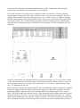
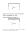
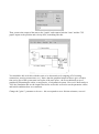
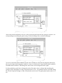
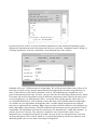
A Simulink Tutorial
(www.cee.uc.edu/~juber/e_reserves/cee627/simulink_tut1.html)
With simulink building a dynamic model can actually be fun. It is also powerful enough to do real
work, once you learn some of its advanced features (i.e., it is not a waste of time to learn). In fact,
we will only use some of the rather basic features of simulink for the models we build, and you are
free (and encouraged) to explore some other features that will help you with problems you want to
solve. Basically you can think of a simulink model as like describing a wiring diagram of your
system, where the variables flow on wires and are changed, or transformed, by various devices.
(The notes on the spring-mass system provide perhaps a better brief introduction to this idea.) Let's
build a simulink model for the linear spring-mass system with viscous damping:
x1
x 2
x2
k
x1
m
k1
x2
m
First, you need to start the matlab application, which you do in Unix by typing "matlab" at the shell
prompt, or in Windows by double-clicking (rapidly clicking the left mouse button twice) on the
matlab icon, which you will find buried somewhere with a bunch of other icons. This will get you to
the ">>" matlab prompt. Type "simulink" to start simulink, and bring up the main simulink window
(your windows may look somewhat different, depending on the machine and operating system):
Let's go though the basic functions of this window first. On top is a list of items that are associated
with pull-down menus. These will be duplicated on your model workspace (see below), so for the
most part they are not too important here. Exept for the "file" menu, which you will use to create a
new model workspace or to bring up a file browser to access an existing (saved) model.
Each of the block icons correspond to a category of transformations that will be used to describe the
dynamic system. You will mostly use the transformations described in "Sources," "Sinks," "Linear,"
"Nonlinear," and "Connections." The "Sources" icon contains a suite of signal generators, such as
random number generators and wave (sinusoidal, square, etc.) generators, that can be used to
provide time-varying inputs that drive your dynamic system (these are exogenous inputs, or external
inputs, meaning that their dynamics are described externally to the model). The "Sinks" category
will mainly be used to access the "Scope" and XY graphs to which you will connect the system
"wires" to get a "readout." The "Linear" category contains all the possible ways to transform a
variable linearly, such as different types of gains. It also has the basic "integrator" block that we
will use extensively to model our first-order dynamic systems. The "nonlinear" block contains
1
various specific and general nonlinear transformations, and the "connections" block includes
various ways to connect the wires and blocks in your diagram.
Now what we'd like to do is open a new workspace to start a new model. To do this, press the
mouse button to bring up the "file" menu, and select "new" to create a new workspace. You'll be
prompted later to name the model when you want to save it. What you'll get is a blank workspace
with the same headings as the main simulink window. Now go up to the main window and doubleclick on the "linear" icon, which will bring up another window containing all the possible linear
transformations. Arrange these three windows how you want them. You'll get something like the
following:
Actually, you'll not have the integrator block in your model workspace yet. To get it there is simple
- just press (and hold) the left mouse button over the integrator block, and then "drag" a copy over
the to workspace wherever you want it to be (don't worry, you can move it again in just the same
way). Go ahead and do this now.
But why did we start with the integrator block? You'll recall that the integrator integrates its input to
produce its output. Thus if the input is dx/dt then the output is x. What we are going to do first is
graphically build the right hand side of the second ordinary differential equation (o.d.e.) listed
above. This will be what goes into the left side of the integrator block, and then what comes out the
right side will be x2. Got it? So, let's proceed to build up the right hand side of this o.d.e., which is
just the linear summation of the two state variables x1 and x2. So what we'll need is two gain blocks
and a sum block to sum the result. The sum block will be first because it assembles the two parts of
2
dx2/dt. So drag a "sum" block over from the "linear" menu and position it to the left of the
integrator:
How did the connecting line get there? Easy, just use the mouse, and first click on the output side of
the sum block (the little "out" arrow) and next on the input side of the integrator (i.e., from tail to
head of the vector). Go ahead and do that. Next, notice that the sum block by default has two inputs
and both are added together. We want two inputs, but we want them to be subtracted (this is
because we want the constants k/m and k1/m to be positive, as by convention we often wish that
model parameters are positive). So, to open up the "sum" dialog box, double-click on it - you'll get
the following:
Notice that you can change the number of inputs by simply editing the number of +/- signs that
appear in the list. Change the two "+" signs to two "-" signs and then select "done" to close the
dialog input. This is the way (double-clicking on an icon) that you bring up the dialog box for any
icon. Each icon has its own dialog box for changing parameters and describing briefly its function.
The "help" button gives a bit more detail, but to really know what each icon does in detail, you'll
have to consult the simulink reference guide. For our purposes we'll mostly be able to go on the
brief help that is available on the dialog.
Now we're going to get some more practice connecting blocks and just using the simulink interface.
First, drag two "gain" blocks from the linear library to the workspace. Alternatively, you can drag
one block over and then press and hold the right mouse button over the gain block to drag a copy of
it. This is sometimes useful since then the new block will have the same parameter values of its
parent. Connect both the gain blocks to the sum block in the usual way. You should get something
like this:
3
Notice that the lower connection between "gain 1" and "sum" is highlighted with little square
blocks. These are significant, and are called "handles." You can deselect that line by clicking the
mouse button on the white background (on nothing), or you can select a different line (show its
handles) by clicking on the desired line. Anyway, the significance of the handles is how they allow
you to move the position of the connection, to make it look better.
For example, positioning the mouse pointer on one of the handles and dragging it repositions only
that vertex of the connection, with the other lines stretching to meet it:
But sometimes you'd rather move an entire line, without changing its orientation. To do this, select
a connection segment that terminates in a handle at each end. Then drag it to its new position, like
this (I moved the vertical line between the gain and the sum blocks):
4
Another thing that is useful to do is create a new line from an existing one (i.e., "tap" into a line
with a bit of solder). This is easy to do - just position the pointer where you want to create the new
line and drag the right mouse button - this creates a new connection oriented vertically,
horizontally, or at a 45 degree angle, depending on which direction you drag. Experiment with this.
Once you release the mouse button, you are left with a line segment with an arrow on the end
(presuming you didn't connect the line to another block yet). You can then select this arrow just like
the output of a block to draw another line segment, perhaps in another direction. Practice this selecting the arrow and dragging the mouse and releasing the mouse button, and doing it again in
another direction. Perhaps you'll end up with something like this:
Which I really don't want there at all, because the mass spring model doesn't require a second
output from the gain 1 block. To get rid of it, just select it (showing its handles) and then select
"cut" from the "edit" menu along the window border. (You can experiment with the other "edit"
functions.) This works in general - for any connection and any block.
What happened to the first "gain" block? It is now about twice its original size. That's just to
illustrate that you can also change the size of the block icons too, in the same way. Just select the
icon (showing its four handles at the corners) and drag one of the handles to size the icon how you
5
want it. You can also drag the icon whereever you want it by selecting not a single handle, but
dragging the body of the icon to where you want it. The connections move along with it.
Now let's just finish off the diagram, since we know pretty much how to use the simulink interface.
Now we said before that the output from the integrator block was going to be x2. Thus if we were to
assign the "gain 1" block to be the viscous damping (a constant times the velocity - or x2) then we
want to have a connection from the output of the integrator to the input of "gain 1". Do this now,
and then position the line to where you'd like it.
But now what is the input to the "gain" block - the position of the mass, or x1? Well, this has to be
constructed as the integration of dx1/dt, or the right hand side of the first o.d.e. above - which is just
x2. Thus we need to drag another integrator block over and connect that as well to the output of the
first integrator block. Do this, and then connect the output of the second integrator block to the
"gain" block, so the diagram looks something like this:
Now stop and convince yourself that the above graphical depiction is actually and accurate
representation of the dynamical system we are trying to solve. You'll notice that I've put in labels
for the two main lines in the diagram - a feature that is usually helpful. And easy. Just click the left
mouse button about where you want the text, and then start typing. You can then move the selected
text just like you can move a block (actually, it is a "text" block).
While you're at it, open up the "output" and the "connections" icons, and select the "mux"
multiplexer block, the "graph" block, and the "XY graph" block, as shown above. The "mux" block
just takes multiple inputs and produces a single - vector - output. This is handy because most
simulink blocks can handle vector inputs as well as scalar inputs, and sometimes it is useful or
essential to have connections carry vector quantities. For example, what we will do is to multiplex
the two variables, position and velocity, to produce a single output vector containing two elements the position and the velocity. This single vector will be sent to the "graph" block, which is set up to
display any number of signals simultaneously. Thus if we send it a two element vector, it will
display those two as output over time, and if we sent it a 10 element vector it would display all of
those. This is just handier than having two separate graphs, and also teaches us a very powerful
aspect of simulink that you might use to advantage in the future - that most of its blocks can process
vector as well as scalar inputs.
Open up the "mux" dialog and change the number of inputs to 2 instead of 3:
6
Then, connect the output of the mux to the "graph", and connect both the "mux" and the "XY
graph" inputs to the position and velocity lines, something like this:
You should be able to do this with the tools we've discussed so far (tapping off of existing
connections, moving connections, etc.). Notice that the graphical output will now give us both a
time series plot of the system state and a plot of the state space - the two traditionaly ways of
graphically illustrating the orbits, or trajectories, of a dynamical system. Now we're about ready to
"run" the simulation and see the output. But before we do this we need to set the parameter values
and initial conditions how we want them.
Change the "gain 1" parameter to be zero - this corresponds to zero friction resistance, correct?:
7
Also set the initial conditions to be zero velocity and an initial stretch of the spring to position +10 corresponding to stretching the guitar string 10 units, holding it there, and then letting go:
You can see that the initial conditions for the state variables are stored in the integrator blocks. By
the way, the input to the integrator could be a vector, in which case I'd specifiy the initial condition
in matlab matrix notation. I did change the value in the correct integrator block, right?
It's also probably a good idea to change the scale of the plots, since we know that stretching the
spring 10 units will produce a range of positions from -10 to +10 (without friction). Open the dialog
box for the Graph and change it, and verify that the scale for the XY graph (phase space plot) is o.k.
too:
8
In general you also need to set up the simulation parameters for the numerical algorithms used to
integrate the dynamical system to determine the trajectory. Open the "simulation control" dialog by
selecting "parameters" from the "simulation" menu along the top of the window:
Simulink offers you 7 different numerical algorithms. We will learn more about some of these a bit
later. But you need to know that the particular numerical algorithms can make a big difference in
terms of the efficiency with which a problem is solved. The Simulink user's manual has a nice
general introduction to this topic. For now, you can select the 5th order Runge-Kutta scheme, which
is accurate and an efficient method so long as different components of the solution (the state space)
are not changing on very different time scales - one much more rapidly than the others (this is a
very informal definition of "stiff" problems). Note that most of the simulink numerical algorithms
are variable step size algorithms, meaning they take a variable length integration step along the
trajectory to approximate the solution. Bigger steps are taken when the solution is not changing very
much, and smaller steps otherwise. Thus the minimum and maximum step size parameters are usercontrollable. The algorithms will select the actual step size automatically - within these bounds - to
satisfy a local error criterion. The "tolerance" parameter sets a bound on the relative local
integration error, meaning basically the error that can occur at any one integration step. Note that
obviously this kind of error control, which is very useful and practical, can not say much by itself
about the global error over the entire time range of integration.
9
Now you can have some fun - run the simulation by selecting "start" from the "simulation" pulldown menu. Adjust the graph windows as they pop up automatically (and right on top of one
another, on my workstation). For the current parameter values, you'll get something like this:
Where the phase space is on the left and the time-series on the right. You can stop the simulation
any time using the "stop" button on the "simulation" menu, and then start again if you like using
"start". Or, you can restart from the beginning without stopping by selecting "restart." Or, you can
"pause" the solution and then resume from the paused point (not the initial conditions) by using
"pause" and "continue". Another neat trick is to use a floating "scope" block (one that is not
connected) from the "Sinks" library and then when you click any line while a simulation is running,
the scope will change to display the state on the line over time (a disadvantage is that you don't get
any scales, just the signal). It is possible to change simulation (or block) parameters "on the fly"
while a simulation is running, and see the effect. Play with these things for a while, until you get
bored with this example.
How about printing a graph of the solution? The best way is to run a simulation and place the values
of the state variables, along with the time of the simulation, on the matlab workspace. This gives
you all the flexibility of matlab with which to process the graphics. Let's learn by an example. First
open the "Sinks" icon again, and drag over two "to workspace" blocks. Then drag a "clock" block
from the "Sources" library. Connect them up like the following:
10
This will take the vector output of the state from the output of the "mux" block and put it into a
matrix variable named 'x' available from the matlab workspace (as usual, you open the "to
workspace" block to set the name of the variable). Similarly, the output of the "clock" icon, which
you can think of as a timer that runs exactly at the simulation speed, is put into a vector variable
named 't' that is available from the matlab workspace. Run the simulation again now, and stop it
after some time.
Go to the main matlab workspace window, and type the command 'whos'. This should show the
variables that are now available. Then type the command 'plot(t,x)' which will plot the time versus
each state variable (which are each stored as a column in the matrix 'x'). See the plot? O.K., now
you can just type 'print' and that plot will be sent to the default printer. You can type 'help print' in
the matlab workspace for details about options. (and also 'help plot' for details about the 'plot'
command).
11