Download HP1 Tutorials II - PC

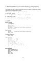
HP1 Tutorials II
(HYDRUS-1D + PHREEQC)
0.0014
Concentration [mol/kg]
0.0012
0.001
Cl
0.0008
Ca
Na
0.0006
K
0.0004
0.0002
0
0
14400
28800
43200
57600
72000
86400
Time [s]
Diederik Jacques* and Jirka Šimůnek#
*
Waste and Disposal, SCK•CEN, Mol, Belgium
#
Department of Environmental Sciences
University of California, Riverside, USA
November, 2009
PC-Progress, Prague, Czech Republic
© 2009 J. Šimůnek. All rights reserved.
2
List of Tutorials:
Table of Contents
3
Abstract
4
1. HP1 Tutorial 1: Transport and Dissolution of Gypsum and Calcite 5
1.1. Input
1.2. Output
1.3. Overview of Selected Results: Profile Data
1.4. Overview of Selected Results: Time Series
2. HP1 Tutorial 2: Transport and Cation Exchange (a single pulse)
2.1. Input
2.2. Output
5
9
12
13
15
15
19
3. HP1 Tutorial 3: Transport and Cation Exchange (multiple pulses) 20
3.1. Input
3.2. Output
20
22
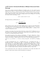
4. HP1 Tutorial 4: Horizontal Infiltration of Multiple Cations and
Cation Exchange
4.1. Definition of the Geochemical Model and its Parameters
4.2. Input
4.3. Output
5. References
23
24
25
30
33
3
Abstract
Jacques, D., and J. Šimůnek, HP1 Tutorials II, PC Progress, Prague, Czech Republic, 2009.
The purpose of this short report is to documents four simple tutorials for the version 2.0 of HP1.
HP1 is a comprehensive modeling tool in terms of available chemical and biological reactions
that was recently developed by coupling HYDRUS-1D with the PHREEQC geochemical code of
Parkhurst and Appelo [1999]. This coupling resulted in the very flexible simulator, HP1, which
is an acronym for HYDRUS1D-PHREEQC [Jacques and Šimůnek, 2005; Jacques et al., 2006].
The combined code contains modules simulating (1) transient water flow in variably-saturated
media, (2) the transport of multiple components, (3) mixed equilibrium/kinetic biogeochemical
reactions, and (4) heat transport. HP1 is a significant expansion of the individual HYDRUS-1D
and PHREEQC programs by combining and preserving most or all of the features and
capabilities of the two codes into a single numerical model. The code uses the Richards equation
for variably-saturated flow and advection-dispersion type equations for heat and solute transport.
However, the program can now simulate also a broad range of low-temperature biogeochemical
reactions in water, the vadose zone and in ground water systems, including interactions with
minerals, gases, exchangers, and sorption surfaces, based on thermodynamic equilibrium,
kinetics, or mixed equilibrium-kinetic reactions. Various additional applications of HP1 were
presented by [Jacques and Šimůnek, 2005, and Jacques et al., 2006, 2008a,b].
Four tutorials are currently presented in this report. The first tutorial involves the Transport and
Dissolution of Gypsum and Calcite, the second and third tutorials the Transport and Cation
Exchange during a single pulse and multiple pulses, respectively; and finally the fourth tutorial
involves Horizontal Infiltration of Multiple Cations and Cation Exchange. More tutorials will be
included in future versions of this brief report.
4
1. HP1 Tutorial 1: Transport and Dissolution of Gypsum and Calcite
Sulfate-free water is infiltrated in a 50-cm long homogeneous soil column under steady-state
saturated flow conditions. The reactive minerals present in the soil column are calcite (CaCO3)
and gypsum (CaSO4.2H2O), both at a concentration of 2.176 x 10-2 mmol/kg soil.
Physical properties of the soil column are as follows:
Porosity = 0.35
Saturated hydraulic conductivity = 10 cm/day
Bulk density = 1.8 g/cm³
Dispersivity = 1 cm.
The input solution contains 1 mM CaCl2 and is in equilibrium with the atmospheric partial
pressure of oxygen and carbon dioxide. The initial soil solution is in equilibrium with the
reactive minerals and with the atmospheric partial pressure of oxygen. As a result of these
equilibria, the initial soil solution contains only Ca and oxidized components of S and C.
Calculate the movement of dissolution fronts of calcite and gypsum over a period of 2.5 days.
1.1. INPUT
Project Manager
Button: "New"
Name: "HP1-1"
Description: "Dissolution of calcite and gypsum in the soil profile"
Button: "OK"
Main Processes
Heading: Dissolution of calcite and gypsum in the soil profile
Uncheck: "Water Flow" (Note: this is a steady-state water flow)
Check: "Solute Transport"
Select: "HP1 (PHREEQC)"
Button: "Next"
Geometry Information
Depth of the Soil Profile: 50 (cm)
Button: "Next"
Time Information
Final Time: 2.5 (days)
Maximum Time Step: 0.05
Button: "Next"
Print Information
Unselect: T-Level information
5
Select: Print at Regular Time Interval
Time Interval: 0.025 (d)
Print Times: Number of Print times: 5
Button: "Next"
Print Times
Button: "Default"
Button: "OK"
HP1 – Print and Punch Controls
Check: "Make GNUplot Templates"
This allows easy visualization of time series and profile data for variables, which are
defined in the SELECTED_OUTPUT section below in this dialog window and also
defined later in the Additional Output part of the Solute Transport – HP1
Definitions dialog.
Button: "Next"
Water Flow – Iteration Criteria
Button: "Next"
Water Flow – Soil Hydraulic Model
Button: "Next"
Water Flow – Soil Hydraulic Parameters
Qs: 0.35
Ks: 10 (cm/d)
Button: "Next"
Water Flow – Boundary Conditions
Upper Boundary Condition: Constant Pressure Head
Lower Boundary Condition: Constant Pressure Head
Button: "Next"
Solute Transport – General Information
Stability Criteria: 0.25 (to limit the time step)
Number of Solutes: 6
Button: "Next"
Solute Transport – HP1 Components and Database Pathway
Six Components: Total_O, Total_H, Ca, C(4), Cl, S(6)
Note: Redox sensitive components should be entered with the secondary master species,
i.e., with their valence state between brackets. The primary master species of a redox
sensitive component, i.e., the element name without a valence state, is not recognized as a
component to be transported. Therefore, the primary master species C can not be entered
here; one has to enter either C(4) or C(-4). Also S is not allowed; one has to enter either
6
S(6) or S(-2). Note that the HYDRUS GUI will not check if a correct master species is
entered. Because the redox potential is high in this example (a high partial pressure of
oxygen), the secondary master species C(-4) and S(-2) are not considered.
Check: "Create PHREEQC.IN file using HYDRUS GUI"
Button: "Next"
Solute Transport – HP1 Definitions
Definitions of Solution Composition
Define the initial condition, i.e., the solution composition of water in the soil
column, with the identifier 1001:
• Pure water
• Bring it in equilibrium with gypsum, calcite, and O(0), to be in
equilibrium with the partial pressure of oxygen in the atmosphere
Define the boundary condition, i.e., the solution composition of water entering the
soil column, with the identifier 3001:
• Ca-Cl solution
• Use pH to obtain the charge balance of the solution
• Adapt the concentration of O(0) and C(4) to be in equilibrium with the
atmospheric partial pressure of oxygen and carbon dioxide, respectively
solution 1001
equilibrium_phases 1001
gypsum
calcite
O2(g) -0.68
save solution 1001
end
solution 3001
-units mmol/kgw
pH 7 charge
Cl 2
Ca 1
O(0) 1 O2(g) -0.68
C(4) 1 CO2(g) -3.5
Button: "OK"
Geochemical Model
Define for each node the geochemical model. Note that the initial amount of a
mineral must be defined as mol/1000 cm³ soil (i.e., 2.176 x 10-5 mol/kg soil * 1.8
kg/1000 cm³).
7
Equilibrium_phases 1-101
gypsum 0 3.9E-5
calcite 0 3.9E-5
O2(g) -0.68
Button: "OK"
Additional Output
Define the additional output to be written to selected output files.
selected_output
-totals Ca Mg Cl S C
-equilibrium_phases gypsum calcite
Button: "OK"
Button: "Next"
Solute Transport – Solute Transport Parameters
Bulk D. = 1.8 (g/cm³)
Disp: 1 cm
Button: "Next"
Solute Transport – Boundary Conditions
Upper Boundary Condition
Bound. Cond. 3001
Soil Profile – Graphical Editor
Menu: Conditions -> Initial Conditions -> Pressure Head
Button: "Edit Condition"
Select All
Top Value: 0
Menu: Conditions -> Observation Points
Button: "Insert"
Insert 5 observation nodes, one for every 10 cm
Menu: File -> Save Data
Menu: File –> Exit
Soil Profile – Summary
Button: "Next"
Run Application
8
1.2. OUTPUT
The standard HYDRUS output can be viewed using commands in the right Post-Processing part
of the project window. Only the total concentrations of the components, which were defined in
“Solute Transport – HP1 Components” can be viewed using the HYDRUS-GUI.
HP1 creates a number of additional output files in the project folder. The path to the project
folder is displayed in the Project Manager:
File -> Project Manager
Directory: gives the path to the project group folder
Input and output files of a given project are in the folder: directory\project_name
where
directory is the project group folder
project is the project name
Following HP1 output files are created for the HP1-1 project:
Createdfiles.out
Phreeqc.out
HP1-1.hse
An ASCII text file containing a list of all files created by HP1 (in
addition to the output files created by the HYDRUS module of
HP1);
An ASCII text file, which is the standard output file created by the
PHREEQC-module in HP1;
An ASCII text file, tab-delimited, that includes a selected output of
all geochemical calculations in HP1 carried out before actual
transport calculations. Inspection of this file can be done with any
spreadsheet, such as MS Excel;
obs_nod_chem21.out
obs_nod_chem41.out
obs_nod_chem61.out
obs_nod_chem81.out
obs_nod_chem101.out A series of ASCII files, tab-delimited, with the selected output for
the defined observation nodes (21, 41, 61, 81, and 101) at specific
times (every 0.025 days). Numerical values can be seen by opening
this file in a spreadsheet, such as Excel. A single plot of time series
at five observation nodes can be generated for each geochemical
variable with the ts_*.plt files using the GNUPLOT graphical
program (see below);
nod_inf_chem.out
An ASCII file, tab-delimited, with the selected output for a
complete soil profile at the defined observation times. Numerical
values can be seen by opening this file in a spreadsheet such as
Excel. A single plot of the profile data at different observation
times can be generated for each geochemical variable with the
pd_*.plt files using GNUPLOT (see below);
ts_pH.plt
pd_pH.plt
9
ts_pe.plt
pd_pe.plt
ts_tot_Ca.plt
pd_tot_Ca.plt
ts_tot_Cl.plt
pd_tot_Cl.plt
ts_tot_S.plt
pd_tot_S.plt
ts_tot_C.plt
pd_tot_C.plt
ts_eq_gypsum.plt
pd_eq_gypsum.plt
ts_eq_calcite.plt
pd_eq_calcite.plt
ts_d_eq_gypsum.plt
pd_d_eq_gypsum.plt
ts_d_eq_calcite.plt
pd_d_eq_calcite.plt
An ASCII file containing command line instructions to generate a
plot of pH or pe using GNUPLOT;
An ASCII file containing command line instructions to generate a
plot with total concentrations of Ca, Cl, S and C using GNUPLOT;
note that this information can also be viewed using the HYDRUS
GUI;
An ASCII file containing command line instructions to generate a
plot with the amount of the minerals gypsum and calcite with
GNUPLOT;
An ASCII file containing command line instructions to generate a
plot with the change in amount of the minerals gypsum and calcite
with GNUPLOT;
To view these various plots, the GNUPLOT code needs to be installed on your computer.
GNUPLOT is freeware software that can be downloaded from http://www.gnuplot.info/. Note
that GNUPLOT (the wgnuplot.exe program for the Windows OS) is usually, after being
downloaded, in the gnuplot\bin folder and does not require any additional special installation.
After opening the Windows version of GNUPLOT by clicking on wgnuplot.exe, a plot can be
directly generated by carrying out these commands:
File->Open
Browse to the project folder
Open the template file of interest (*.plt)
The figure can be adapted using line commands (see tutorials on the internet). After adaptations,
the command lines can be saved to be used later on.
The default terminal for the plots is Window. We illustrate here only how a plot can be
transferred to another terminal:
Set terminal emf
10
Set output "name.emf"
Replot
Set terminal window
Replot
A name.emf file is created in the project directory.
11
0
0
-10
-10
Distance (cm)
Distance (cm)
1.3. Overview of Selected Results: Profile Data
-20
-30
-50
-50
5.5
6
6.5
0 days
0.50 days
7
7.5
pH
8
8.5
9
1.00 days
1.50 days
5.5
9.5
6
6.5
0 days
0.50 days
2.00 days
2.50 days
0
0
-10
-10
Distance (cm)
Distance (cm)
-30
-40
-40
-20
-30
-40
7
7.5
pH
1.00 days
1.50 days
8
8.5
9
9.5
2.00 days
2.50 days
-20
-30
-40
-50
-50
0
0.004
0.008
0.012
Total concentration of Ca (mol/kg water)
0 days
0.50 days
1.00 days
1.50 days
0.016
0
0.004
0.008
0.012
Total concentration of S (mol/kg water)
0 days
0.50 days
2.00 days
2.50 days
0
0
-10
-10
Distance (cm)
Distance (cm)
-20
-20
-30
-40
1.00 days
1.50 days
0.016
2.00 days
2.50 days
-20
-30
-40
-50
-50
0
1e-005
2e-005
3e-005
gypsum (mol/1000 cm³ of soil)
0 days
0.50 days
1.00 days
1.50 days
4e-005
0
1e-005
0 days
0.50 days
2.00 days
2.50 days
2e-005
3e-005
4e-005
calcite (mol/1000 cm³ of soil)
1.00 days
1.50 days
5e-005
2.00 days
2.50 days
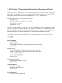
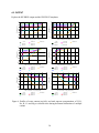
Figure 1. Profiles of pH (top left), total aqueous C concentration (top right), total aqueous Ca
concentration (middle left), total aqueous S concentration (middle right), the amount
of gypsum (bottom left) and the amount of calcite (bottom right) at selected print
times during dissolution of calcite and gypsum.
12
Total concentration of C (mol/kg water)
1.4. Overview of Selected Results: Time Series
9.5
9
8.5
pH
8
7.5
7
6.5
6
5.5
0
0.5
1
1.5
Time (days)
0.008
0.004
0
1
1.5
Time (days)
-10.0 cm
-20.0 cm
-30.0 cm
2e-005
1e-005
0
2
2.5
0.5
1
1.5
Time (days)
2
2.5
-40.0 cm
-50.0 cm
0.016
0.012
0.008
0.004
0
0
0.5
1
1.5
Time (days)
-10.0 cm
-20.0 cm
-30.0 cm
-40.0 cm
-50.0 cm
2
2.5
-40.0 cm
-50.0 cm
5e-005
calcite (mol/1000 cm³ of soil)
4e-005
gypsum (mol/1000 cm³ of soil)
3e-005
-10.0 cm
-20.0 cm
-30.0 cm
0.012
0.5
4e-005
-40.0 cm
-50.0 cm
0.016
0
5e-005
2.5
Total concentration of S (mol/kg water)
Total concentration of Ca (mol/kg water)
-10.0 cm
-20.0 cm
-30.0 cm
2
6e-005
3e-005
2e-005
1e-005
4e-005
3e-005
2e-005
1e-005
0
0
0
0.5
-10.0 cm
-20.0 cm
-30.0 cm
1
1.5
Time (days)
2
2.5
0
0.5
-10.0 cm
-20.0 cm
-30.0 cm
-40.0 cm
-50.0 cm
1
1.5
Time (days)
2
2.5
-40.0 cm
-50.0 cm
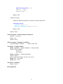
Figure 2. Time series of pH (top left), total aqueous C concentration (top right), total aqueous
Ca concentration (middle left), total aqueous S concentration (middle right), the
amount of gypsum (bottom left) and the amount of calcite (bottom right) at selected
depths (observation nodes) during dissolution of calcite and gypsum.
13
14
2. HP1 Tutorial 2: Transport and Cation Exchange (a single pulse)
This example is adapted from Example 11 of the PHREEQC manual [Parkhurst and Appelo,
1999]. We will simulate the chemical composition of the effluent from an 8-cm column
containing a cation exchanger. The column initially contains a Na-K-NO3 solution in equilibrium
with the cation exchanger. The column is flushed with three pore volumes of a CaCl2 solution.
Ca, K and Na are at all times in equilibrium with the exchanger. The simulation is run for one
day; the fluid flux density is equal to 24 cm/d (0.00027777 cm/s).
The column is discretized into 40 finite elements (i.e., 41 nodes). The example assumes that the
same solution is initially associated with each node. Also, we use the same exchanger
composition for all nodes.
The initial solution is Na-K-NO3 solution is made by using 1 x 10-3 M NaNO3 and 2 x 10-4 M
KNO3 M. The inflowing CaCl2 solution has a concentration of 6 x 10-4 M. Both solutions were
prepared under oxidizing conditions (in equilibrium with the partial pressure of oxygen in the
atmosphere). The amount of exchange sites (X) is 1.1 meq/1000 cm³ soil. The log K constants
for the exchange reactions are defined in the PHREEQC.dat database and do not have to be
therefore specified at the input.
In this example, only the outflow concentrations of Cl, Ca, Na, and K are of interest.
2.1. INPUT
Project Manager
Button "New"
Name: CEC-1
Description: Transport and Cation Exchange, a single pulse
Button "OK"
Main Processes
Heading: Transport and Cation Exchange, a single pulse
Uncheck "Water Flow" (steady-state water flow)
Check "Solute Transport"
Select “HP1 (PHREEQC)”
Button "Next"
Geometry Information
Depth of the soil profile: 8 (cm)
Button "Next"
Time Information
Time Units:
Final Time:
Seconds (Note that you can also just put it in days, this would also
be OK)
86400 (s)
15
Initial Time Step:
180
Minimum Time Step: 180
Maximum Time Step: 180 (Note: constant time step to have the same conditions as in
the original comparable PHREEQC calculations).
Button "Next"
Print Information
Number of Print Times: 12
Button "Select Print Times"
Button "Next"
Print Times
Button: "Default"
Button: "OK"
HP1 – Print and Punch Controls
Button: "Next
Water Flow - Iteration Criteria
Lower Time Step Multiplication Factor: 1
Button "Next"
Water Flow - Soil Hydraulic Model
Button "Next"
Water Flow - Soil Hydraulic Parameters
Catalog of Soil Hydraulic Properties: Loam
Qs: 1 (Note: to have the same conditions as in the original comparable PHREEQC
calculations)
Ks: 0.00027777 (cm/s)
Button "Next"
Water Flow - Boundary Conditions
Upper Boundary Condition: Constant Pressure Head
Lower Boundary Condition: Constant Pressure Head
Button "Next"
Solute Transport - General Information
Number of Solutes: 7
Button "Next"
Solute Transport – HP1 Components and Database Pathway
Add seven components: Total_O, Total_H, Na, K, Ca, Cl, N(5)
Check: "Create PHREEQC.IN file Using HYDRUS GUI"
Button: "Next"
16
Solute Transport – HP1 Definitions
Definitions of Solution Composition
Define the initial condition 1001:
• K-Na-N(5) solution
• use pH to charge balance the solution
• Adapt the concentration of O(0) to be in equilibrium with the partial
pressure of oxygen in the atmosphere
Define the boundary condition 3001:
• Ca-Cl solution
• Use pH to charge balance the solution
• Adapt the concentration of O(0) to be in equilibrium with the partial
pressure of oxygen in the atmosphere
Solution 1001 Initial condition
-units mmol/kgw
pH 7 charge
Na 1
K 0.2
N(5) 1.2
O(0) 1 O2(g) -0.68
Solution 3001 Boundary solution
-units mmol/kgw
pH 7 charge
Ca 0.6
Cl 1.2
O(0) 1 O2(g) -0.68
Geochemical Model
Define for each node (41 nodes) the geochemical model, i.e., the cation exchange
assemblage X (0.0011 moles / 1000 cm³) and equilibrate it with the initial
solution (solution 1001).
EXCHANGE 1-41 @Layer 1@
X 0.0011
-equilibrate with solution 1001
Button: "OK"
Additional Output
Since output is required only for the total concentrations and such output is
available in the automatically generated file obs_node.out, there is not need to
define additional output.
Button: "Next"
17
Solute Transport - Transport Parameters
Bulk Density: 1.5 (g/cm3)
Disp.:
0.2 (cm)
Button "Next"
Solute Transport - Boundary Conditions
Upper Boundary Condition:
Concentration Flux
Add the solution composition number (i.e., 3001) for the upper boundary condition
Lower Boundary Condition:
Zero Gradient
Button "Next"
Soil Profile - Graphical Editor
Menu: Conditions->Profile Discretization
or Toolbar: Ladder
Number (from sidebar):
41
Menu: Conditions->Initial Conditions->Pressure Head
or Toolbar: red arrow
Button "Edit condition", select with Mouse the entire profile and specify 0 cm pressure
head.
Menu: Conditions->Observation Points
Button "Insert", Insert a node at the bottom
Menu: File->Save Data
Menu: File->Exit
Soil Profile - Summary
Button "Next"
Close Project
Run project
Note: This exercise will produce following warnings: "Master species N(3) is present in solution
n but is not transported.". The same warning occurs for N(0). N(3) and N(0) are two secondary
master species from the primary master species N. Only the secondary master species N(5) was
defined as a component to be transported (Solute Transport – HP1 Components). HP1, however,
checks if all components, which are present during the geochemical calculations, are defined in
the transport model. If not, a warning message is generated. In our example, the concentrations
of the components N(0) and N(3) are very low under the prevailing oxidizing conditions.
Therefore, they can be neglected in the transport problem. If you want to avoid these warnings,
you have to either include N(0) and N(3) as components to be transported or define an alternative
using
primary
master
species
representing
nitrate
(such
as
Nit-)
SOLUTION_MASTER_SPECIES and SOLUTION_SPECIES.
18
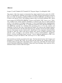
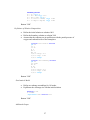
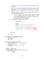
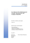
2.2. OUTPUT
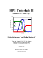
Display results for “Observation Points” or “Profile Information”. Alternatively, the Figure 3
graph can be created using information in the output file obs_nod.out.
0.0014
Concentration [mol/kg]
0.0012
0.001
Cl
0.0008
Ca
Na
0.0006
K
0.0004
0.0002
0
0
14400
28800
43200
57600
72000
86400
Time [s]
Figure 3. Outflow concentrations of Cl, Ca, Na and K for the
single-pulse cation exchange example.
Results for this example are shown in Figure 3, in which concentrations for node 41 (the last
node) are plotted against time. Chloride is a conservative solute and arrives in the effluent at
about one pore volume. The sodium initially present in the column exchanges with the incoming
calcium and is eluted as long as the exchanger contains sodium. The midpoint of the
breakthrough curve for sodium occurs at about 1.5 pore volumes. Because potassium exchanges
more strongly than sodium (larger log K in the exchange reaction; note that log K for individual
pairs of cations are defined in the database and therefore did not have to be specified), potassium
is released after sodium. Finally, when all of the potassium has been released, the concentration
of calcium increases to a steady-state value equal to the concentration of the applied solution.
19
3. HP1 Tutorial 3: Transport and Cation Exchange (multiple pulses)
This example is the same as the one described in the previous example, except that time variable
concentrations are applied at the soil surface.
Following sequence of pulses are applied at the top boundary:
0 – 8 hr: 6 x 10-4 M CaCl2
8 – 18 hr: 5 x 10-6 M CaCl2, 1 x 10-3 M NaNO3, and 2 x 10-4 M KNO3
18 – 38 hr: 6 x 10-4 M CaCl2
38 – 60 hr: 5 x 10-6 M CaCl2, 1 x 10-3 M NaNO3, and 8 x 10-4 M KNO3
3.1. INPUT
Project Manager
Click on CEC-1
Button "Copy"
New Name: CEC-2
Description: Transport and Cation Exchange, multiple pulses
Button "OK", "Open"
Main Processes
Heading:
Transport and Cation Exchange, multiple pulses
Button "Next"
Geometry Information
Button "Next"
Time Information
Time Units:
hours
Final Time:
60 (h)
Initial Time Step:
0.1
Minimum Time Step: 0.1
Maximum Time Step:
0.1
Check Time-Variable Boundary Conditions
Number of Time-Variable Boundary Records:
Button "Next"
Print Information
Number of Print Times: 12
Button "Select Print Times"
Default
Button "OK"
Button "Next"
20
4
Solute Transport – HP1 Definitions
Definitions of Solution Composition
Add additional boundary solution compositions with numbers 3002 and 3003.
Define a bottom boundary solution: Solution 4001 – pure water
Solution 3002 Boundary solution
-units mmol/kgw
ph 7 charge
Na 1
K 0.2
N(5) 1.2
Ca 5E-3
Cl 1E-2
O(0) 1 O2(g) -0.68
Solution 3003 Boundary solution
-units mmol/kgw
ph 7 charge
Na 1
K 0.8
N(5) 1.8
Ca 5E-3
Cl 1E-2
O(0) 1 O2(g) -0.68
solution 4001 bottom boundary solution
#pure water
Button: "OK"
Button: "Next"
Time-Variable Boundary Conditions
Fill in the time, and the solution composition number for the top boundary
Time
8
18
38
60
cTop
3001
3002
3001
3003
cBot
4001
4001
4001
4001
Soil Profile - Graphical Editor
Menu: Conditions->Observation Points
Button "Insert", Insert node at 2, 4, 6, and 8 cm
Menu: File->Save Data
Menu: File->Exit
Soil Profile - Summary
Button "Next"
Calculations - Execute HP1
21
3.2. OUTPUT
After the program finishes, explore the output files.
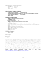
Total concentration of K (mol/kg water)
Figure 4 gives the K concentration at different depths in the profile. Figure 5 shows the outflow
concentration. The first pulse is identical to the single pulse project. Then additional solute
pulses of different solution compositions will restart the cation exchange process depending on
the incoming solution composition.
0.0012
0.001
0.0008
0.0006
0.0004
0.0002
0
0
10
20
30
Time (hours)
40
60
-6.0 cm
-8.0 cm
-2.0 cm
-4.0 cm
Figure 4.
50
Time series of K concentrations at four depths for the
multiple-pulse cation exchange example.
Concentrations (mol/kg water)
0.0012
0.001
0.0008
0.0006
0.0004
0.0002
0
0
10
20
30
Time (hours)
Na
Cl
40
K
50
60
Ca
Figure 5. Outflow concentrations for the multiple-pulse cation
exchange example.
22
4. HP1 Tutorial 4: Horizontal Infiltration of Multiple Cations and Cation
Exchange
This exercise simulates horizontal infiltration of multiple cations (Ca, Na, and K) into the
initially dry soil column. It is vaguely based on experimental data presented by Smiles and Smith
[2004]. The cation exchange between particular cations is described using the Gapon Exchange
equation [White and Zelazny, 1986]. For an exchange reaction on an exchange site X involving
two cations N and M with charge n and m:
N1/nX + 1/m M = M1/mX + 1/n N
(1)
the Gapon selectivity coefficient KGMN is:
[M1 / m X ] ⎡⎢⎣N n + ⎤⎥⎦ 1 / n
K GMN =
[N 1 / n X ] ⎡⎢⎣ M m + ⎤⎥⎦ 1 / m
(2)
where [] denotes activity. The activity of the exchange species is equal to its equivalent fraction.
The Gapon selectivity coefficients for Ca/Na, Ca/K and Ca/Mg exchange are KGCaNa = 2.9, KGCaK
= 0.2, and KGCaMg = 1.2. It is assumed that the cation exchange capacity cT (molckg-1 soil) is
constant and independent of pH.
Consider a soil column 20-cm long with an initial water content of 0.075. Infiltration occurs on
the left side of the column under a constant water content equal to the saturated water content.
Consider a free drainage right boundary condition.
Some physical parameters of the column are: bulk density = 1.75 g/cm³ ; dispersivity = 10 cm ;
the soil water retention characteristic and unsaturated hydraulic conductivity curve are described
with the van Genuchten – Mualem model [van Genuchten, 1980] with following parameters: θs =
0.307, θr = 0 , α = 0.259 cm-1 , n = 1.486 , Ks = 246 cm / day, and l = 0.5. The CEC is 55 meq/kg
soil.
As initial concentrations take: [Cl] = 1 mmol/kg water, [Ca] = 20 mmol/kg water, [K] = 2
mmol/kg water, [Na] = 5 mmol/kg water, [Mg] = 7.5 mmol/kg water, and [C(4)] = 1 mmol/kg
water. The pH is 5.2, and the solution contains an unknown concentration of SO24 as a major
anion. The inflowing solution has the following composition: [Ca] = 0.002345 mol/kg water,
[Na] = 0.01 mol/kg water, [K] = 0.0201 mol/kg water, [Mg] = 0, and [Cl] = 0.035 mol/kgw. The
pH is 3.2, and the solution contains an unknown concentration of SO42- as a major anion.
Look at profile data of the water content, pH, concentrations of the cations and anions, and
amounts of sorbed cations. Express sorbed concentrations in meq/kg soil.
23
4.1. DEFINITION OF THE GEOCHEMICAL MODEL AND ITS PARAMETERS
1. The CEC should be expressed in mol/1000 cm3 soil in HP1. Recalculate the amount of
CEC.
[Answer: 0.09625 mol / 1000 cm³ soil]
2. Define the thermodynamic data for describing the exchange process with the Gapon
convention and the Gapon selectivity coefficients.
A new master exchange species has to be defined, say G.
The exchange reactions (Eq. 1) have to be written in terms of half reactions:
GGGG-
+
+
+
+
K+ = KG
Na+ = NaG
0.5 Ca+2 = Ca0.5G
0.5 Mg+2 = Mg0.5G
(3)
(4)
(5)
(6)
with appropriate values of the exchange coefficients. Thus, log KGK, log KGNa, log KGCa,
and log KGMg are needed for equations 3, 4, 5, and 6, respectively. It is assumed that the
log KG value for the half reaction with Na is 1, i.e., log KGNa = 0.0. The thermodynamic
constants for the other half reactions can then be calculated from the defined Gapon
selectivity coefficients.
Calculate log KGK, log KGCa, and log KGMg.
Solution:
Exchange reactions are written in terms of half reactions. The reaction:
Na-G + 0.5 Ca2+ = Na+ + Ca0.5-G KGCaNa
can be written as the sum of two half reactions:
(1) G- + Na+ = Na-G
(2) G- + 0.5 Ca2+ = Ca0.5-G
KGNa
KGca
Consequently:
log(KGCaNa) = log(KGCa) - log(KGNa)
We express the exchange coefficients relative to Na+. Thus, taking log(KGNa) equals
to 0, log(KGCa) = log(KGCaNa). Similarly, for the reaction:
K-G + 0.5 Ca2+ = K+ + Ca0.5-G KGCaK
24
the following two half reactions can be written:
(1) G- + K+ = K-G
(2) G- + 0.5 Ca2+ = Ca0.5-G
KGK
KGca
Then, log(KGCaK) = log(KGCa) - log(KGK). And similarly, log(KGK) = log(KGCa) log(KGCaK). The same reasoning is applied also to derive KGMg.
[Answer: Log KGK = 1.16
Log KGCa = 0.462
Log KGMg = 0.383]
4.2. INPUT
Project Manager
Button "New"
Name: CEC-3
Description: Horizontal Infiltration with Cation Exchange
Button "OK"
Main Processes
Heading: Horizontal Infiltration with Cation Exchange
Check "Water Flow"
Check "Solute Transport"
Select “HP1 (PHREEQC)”
Button "Next"
Geometry Information
Depth of the soil profile: 20 (cm)
Decline from vertical axes: 0 (horizontal flow)
Button "Next"
Time Information
Time Units:
Minutes
Final Time:
144 (min)
Initial Time Step:
0.01
Minimum Time Step: 0.01
Maximum Time Step: 2
Button "Next"
Print Information
Number of Print Times: 6
Button "Select Print Times"
Button "Default(log)"
Button "OK"
25
Button "Next"
HP1 – Print and Punch Controls
Select: Make GNUPLOT templates
Button: "Next
Water Flow - Iteration Criteria
Lower Time Step Multiplication Factor: 1.3
Button "Next"
Water Flow - Soil Hydraulic Model
Button "Next"
Water Flow - Soil Hydraulic Parameters
Catalog of Soil Hydraulic Properties: Loam
Qr: 0
Qs: 0.307
Alpha: 0.259 (cm-1)
n: 1.486
Ks: 0.170833 (cm/min)
Button "Next"
Water Flow - Boundary Conditions
Initial Conditions: in Water Contents
Upper Boundary Condition: Constant Water Content
Lower Boundary Condition: Free Drainage
Button "Next"
Solute Transport - General Information
Number of Solutes: 9
Button "Next"
Solute Transport – HP1 Components and Database Pathway
Add the nine components: Total_O, Total_H, Ca, Na, K, Mg, Cl, C(4), S(6)
Check: "Create PHREEQC.IN file using HYDRUS GUI"
Button: "Next"
Solute Transport – HP1 Definitions
Additions to Thermodynamic Database
•
•
Define the master exchange species G
Define the master species. An identical reaction for the master exchange
species has to be included.
EXCHANGE_MASTER_SPECIES
G G-
26
EXCHANGE_SPECIES
G- = G-; log_k 0
G- + K+ = KG; log_k 1.16
G- + Na+ = NaG; log_k 0
G- + 0.5 Ca+2 = Ca0.5G; log_k 0.462
G- + 0.5 Mg+2 = Mg0.5G; log_k 0.383
Button: "OK"
Definitions of Solution Compositions
•
•
•
Define the initial solution as solution 1001
Define the boundary solution as solution 3001
Assume that the solutions are in equilibrium with the partial pressure of
oxygen and carbon dioxide of the atmosphere
solution 1001 initial solution
pH 5.2
Cl 1
Ca 20
K 2
Na 5
Mg 7.5
C(4) 1 CO2(g) -3.5
O(0) 1 O2(g) -0.68
S(6) 1 charge
solution 3001 boundary solution
pH 3.2
Ca 2.345
Na 10
K 20
Cl 35
C(4) 1 CO2(g) -3.5
O(0) 1 O2(g) -0.68
S(6) 1 charge
Button: "OK"
Geochemical Model
•
•
Define an exchange assemblage for 101 nodes
Equilibrate the exchange site with the initial solution
Exchange 1-101
G 0.09625
-equilibrate with solution 1001
Button: "OK"
Additional Output
27
•
•
•
Add SELECTED_OUTPUT to ask for output of total concentrations of the
components
Add USER_PUNCH to save the absorbed concentrations as meq/kg soil. The
default output in HP1 for an exchange species is mol/kg water. This can be
asked by –molalities NaG in SELECTED_OUTPUT or as a basic
statement (10 punch mol("NaG")) in USER_PUNCH. Basic statements to
convert 'mol/kg water' to 'meq/kg soil' can be added to USER_PUNCH. The
following two variables are needed:
o The bulk density: use the HP1-specific BASIC statement
bulkdensity(number), where number is the cell number of a given
node, to obtain the bulk density for a given node. The number of the
cell is obtained by the BASIC statement cell_no.
o The water content: obtained as tot("water").
Add meaningful headings for the punch output.
SELECTED_OUTPUT
-totals Cl Ca K Na Mg S
USER_PUNCH
-headings Sorbed_Ca@meq/kg_soil Sorbed_Mg@meq/kg_soil
Sorbed_Na@meq/kg_soil Sorbed_K@meq/kg_soil
-start
10 bd = bulkdensity(cell_no) #kg/1000cm³ soil
40 PUNCH mol("Ca0.5G")*tot("water")/bd*1000 #in meq/kg
50 PUNCH mol("Mg0.5G")*tot("water")/bd*1000 #in meq/kg
60 PUNCH mol("NaG")
*tot("water")/bd*1000 #in meq/kg
70 PUNCH mol("KG")
*tot("water")/bd*1000 #in meq/kg
-end
Button: "OK"
Button: "next"
Solute Transport – Solute Transport Parameters
Bulk Density: 1.75 (g/cm3)
Disp: 10 (cm)
Button "Next"
Solute Transport - Boundary Conditions
Upper Boundary Condition:
Concentration Flux
Bound. Cond.: 3001
Lower Boundary Condition:
Zero Gradient
Button "Next"
Soil Profile - Graphical Editor
Menu: Conditions -> Initial Conditions -> Water content
Button: "Edit Condition"
Select All
28
Top Value: 0.075
Button: "Edit Condition"
Select first node
Value: 0.307
Menu: Conditions -> Observation Points
Button: "Insert"
Insert 4 observation nodes at 3, 6, 9, and 12 cm
Menu: File -> Save Data
Menu: File –> Exit
Soil Profile - Summary
Button "Next"
Calculations - Execute HP1
29
4.3. OUTPUT
0
0
-5
-5
Distance (cm)
Distance (cm)
Explore the HYDRUS output and the GNUPLOT templates.
-10
-15
-15
-20
0.05
-20
0.1
0.15
0.2
0.25
0.3
Mass of water (kg/1000 cm³ of soil)
12.00 min
27.47 min
62.90 min
0
0.35
0
0
-5
-5
-10
-15
0.01
0.015
0.02
0.025
0.03
Total concentration of Cl (mol/kg water)
12.00 min
27.47 min
62.90 min
0.035
144.00 min
-10
-15
-20
0.0045
0.006
0.0075
Total concentration of Na (mol/kg water)
0 min
2.29 min
5.24 min
12.00 min
27.47 min
62.90 min
-20
0.001
0.009
0.002
0.003
0.004
0.005
0.006
0.007
Total concentration of K (mol/kg water)
0 min
2.29 min
5.24 min
144.00 min
0
-5
-5
Distance (cm)
0
-10
-15
-20
0.008
0.005
0 min
2.29 min
5.24 min
144.00 min
Distance (cm)
Distance (cm)
0 min
2.29 min
5.24 min
Distance (cm)
-10
12.00 min
27.47 min
62.90 min
0.008
144.00 min
-10
-15
0.01
0.012
0.014
0.016
0.018
0.02
Total concentration of Ca (mol/kg water)
0 min
2.29 min
5.24 min
12.00 min
27.47 min
62.90 min
0.022
-20
0.003
0.004
0.005
0.006
0.007
Total concentration of Mg (mol/kg water)
0 min
2.29 min
5.24 min
144.00 min
12.00 min
27.47 min
62.90 min
0.008
144.00 min
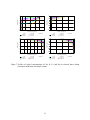
Figure 6. Profiles of water content (top left), and total aqueous concentrations of Cl, K,
Na, K, Ca and Mg at selected times during horizontal infiltration of multiple
cations.
30
0
-5
-5
Distance (cm)
Distance (cm)
0
-10
-15
-15
-20
-20
0.6
0.7
0.8
0.9
Sorbed Na (meq/kg soil)
0 min
2.29 min
5.24 min
12.00 min
27.47 min
62.90 min
1
1.1
3
6
0 min
2.29 min
5.24 min
144.00 min
0
0
-5
-5
Distance (cm)
Distance (cm)
-10
-10
-15
9
Sorbed K (meq/kg soil)
12.00 min
27.47 min
62.90 min
12
15
144.00 min
-10
-15
-20
-20
27
28
0 min
2.29 min
5.24 min
29
30
31
32
Sorbed Ca (meq/kg soil)
12.00 min
27.47 min
62.90 min
33
34
13
14
0 min
2.29 min
5.24 min
144.00 min
15
Sorbed Mg (meq/kg soil)
12.00 min
27.47 min
62.90 min
16
17
144.00 min
Figure 7. Profiles of sorbed concentrations of Na, K, Ca and Mg at selected times during
horizontal infiltration of multiple cations.
31
32
5. References
Jacques, D., and J. Šimůnek, User Manual of the Multicomponent Variably-Saturated Flow and
Transport Model HP1, Description, Verification and Examples, Version 1.0, SCK•CENBLG-998, Waste and Disposal, SCK•CEN, Mol, Belgium, 79 pp., 2005.
Jacques D., J. Šimůnek, D. Mallants, and M. Th. van Genuchten, Operator-splitting errors in
coupled reactive transport codes for transient variably saturated flow and contaminant
transport in layered soil profiles, J. Contam. Hydrology, 88, 197-218, 2006.
Jacques D., J. Šimůnek, D. Mallants, and M. Th. van Genuchten, Modeling coupled hydrological
and chemical processes: Long-term uranium transport following mineral phosphorus
fertilization, Vadose Zone Journal, doi:10.2136/VZJ2007.0084, Special Issue “Vadose Zone
Modeling”, 7(2), 698-711, 2008a.
Jacques D., J. Šimůnek, D. Mallants, and M. Th. van Genuchten, Detailed modeling of coupled
water flow, solute transport and geochemical reactions: Migration of heavy metals in a
podzol soil profile, Geoderma, 145, 449-461, 2008b.
Parkhurst, D. L., and C. A. J. Appelo, User's guide to PHREEQC (Version 2) – A computer
program for speciation, batch-reaction, one-dimensional transport and inverse geochemical
calculations. Water-Resources Investigations, Report 99-4259, Denver, Co, USA, 312 pp,
1999.
Šimůnek, J., M. Šejna, H. Saito, M. Sakai, and M. Th. van Genuchten, The HYDRUS-1D
Software Package for Simulating the Movement of Water, Heat, and Multiple Solutes in
Variably Saturated Media, Version 4.0, HYDRUS Software Series 3, Department of
Environmental Sciences, University of California Riverside, Riverside, California, USA, pp.
315, 2008.
Smiles, D. E., and C. J. Smith, Absorption of artificial piggery effluent by soil: A laboratory
study, Australian J. of Soil Res., 42, 961-975, 2004.
van Genuchten, M. Th., A closed-form equation for predicting the hydraulic conductivity of
unsaturated soils, Soil Sci. Soc. Am. J., 44, 892-898, 1980.
White, N., and L. W. Zelazny, Charge properties in soil colloids, In: Soil Physical Chemistry,
edited by D. L. Sparks, CRC Press, BOCA Raten, Florida, 1986.
33