Download Taylor User`s Manual

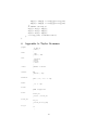
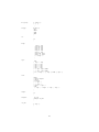
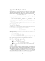
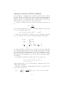
Taylor User’s Manual
Àngel Jorba <[email protected]>
Maorong Zou <[email protected]>
November 13, 2001
1
What is Taylor
Taylor is an ODE solver generator. It reads a system of ODEs and it outputs
an ANSI C routine that performs a single step of the numerical integration of
these ODEs, by means of the Taylor method. Each step of integration chooses
the step and the order in an adaptive way trying to keep the local error below a
given threshold, and to minimize the global computational effort. There is also
support for several extended precision arithmetics.
2
Obtaining Taylor
Taylor is available via anonymous ftp from
ftp://ftp.math.utexas.edu:/pub/mzou
ftp://ftp.maia.ub.es:/pub/angel
(US)
(Europe)
You can also download taylor on the web using the URLs
http://www.math.utexas.edu/users/mzou/taylor/
http://www.maia.ub.es/~angel/taylor/
(US)
(Europe)
Taylor is released under the GNU Public License (GPL), so anybody with
Internet access is free to get it and to redistribute it. The latest version is 1.3.8.
3
Installing Taylor
Taylor runs only on a Unix system. It has been tested under Linux, SunOS
and Solaris. It should compile and run on other variant of unices.
After downloading the distribution taylor-x.y.z.tgz, where x.y.z is the
version number, unpack the archive using the command
tar xvzf taylor-x.y.z.tgz
or, if your version of tar does not handle compressed files, you can also use
gzip -dc taylor-x.y.z.tgz | tar xvf 1
This will create a directory Taylor-x.y. Change to this directory.
Now, to compile taylor, run make. It will produce the executable taylor in
the current directory. You need an ANSI C compiler and lex/yacc parser generator to compile taylor. Using gcc and flex/bison is highly recommended.
To install taylor, simply copy the executable taylor and the manual page
src/taylor.1 to their destination directories. You can put the binary in one
of your directories or, if you have the right permissions, in a system directory,
cp taylor /usr/local/bin/taylor
In this case, you may also want to install the man page,
cp src/taylor.1 /usr/local/man/man1/taylor.1
4
Running Taylor
4.1
Input Syntax
To use taylor, the first order of business is to prepare an input ASCII file with
the system of ODEs. Input to taylor consists of statements of the form
id = expr;
diff(var, tvar) = expr;
where tvar is the time variable and expr is a valid mathematical expression
made from numbers, the time variable, the state variables, elementary functions
sin, cos, tan, arctan, sinh, cosh, tanh, exp, and log, using the four arithmetic
operators and function composition. For example
a = sin(1) + log(1 + exp(-0.5));
b = a + cos(0.1);
c = a+b;
ff = sin(x+t) * exp(-x*x);
diff(x,t) = c * ff - tan(t);
are all valid statements.
Taylor also understands if-else expressions and non-nested sums. For
example, taylor accepts the following statements:
ss = sum( i*sin(i * x)+ i *cos(i*t), i=1,10);
diff(x,t) = ss;
diff(y,t) = if(y>t) { if(y>0.0) { y } else { 1-y }
else
{ y+t};
}
The detailed input syntax is given in Appendix A.
4.2
Overall
Once the input file is ready, there are two main steps in the construction of the
Taylor integrator.
2
First, we should ask taylor to produce the code to compute the jet of derivatives and the automatic step size (and degree) control. This code is arithmeticindependent, in the sense that the real numbers are declared as MY FLOAT (type
to be defined later) and the arithmetic operations have been replaced by C
macros. Hence, the selection of basic arithmetic only depends on the definition
of these macros.
The second step is to ask taylor to produce a header file with a concrete
definition of the type MY FLOAT and the macros that define the basic arithmetic.
This file is included by the previous C file with the jet of derivatives and the
step size control, so that the C preprocessor can substitute these macros by the
code for the desired arithmetic.
We provide header files to use some extended precision arithmetics (later
we give a concrete list), but none of these libraries is included in the taylor
package; the user is supposed to retrieve and install them separately.
To use an arithmetic different from the ones mentioned here, the user only
needs to introduce the corresponding function calls in the header file.
The two previous steps can be combined in a single one, by asking taylor
to put everything (jet, step size and headers) in a single file.
The next section contains a simple example, using the standard double precision of the computer. Next, in Section 5.2, we will show all the options of the
taylor program.
4.3
Example 1
Let’s save the next four lines in the ASCII file lorenz.eq1. It specifies the
famous Lorenz equation.
RR = 28.0;
diff(x,t) = 10.0* (y - x);
diff(y,t) = RR * x - x*z - y;
diff(z,t) = x* y - 8.0* z /3.0;
After saving the file lorenz.eq1, let’s ask taylor to generate a solver for us. A
first possibility is to invoke taylor as follows
taylor -name lrnz -o lorenz.c -jet -step lorenz.eq1
taylor -name lrnz -o taylor.h -header
The first line creates the file lorenz.c (-o flag) with the code that computes the
jet of derivatives (-jet flag) and the step size control (-step flag); the ODE
description is read from the input file lorenz.eq1. The flag -name is to tell
taylor the name we want for the function that performs a single step of the
numerical integration; in this case the name is taylor step lrnz (the string
after the -name flag is appended to the string taylor step to get the name
of this function). The detailed description of the parameters of this function
is in Section 5.3. The second line produces a header file (named taylor.h)
needed to compile lorenz.c, that also contains the prototypes of the functions
3
in lorenz.c (this is the reason for using again the flag -name) so the user may
also want to include it to have these calls properly declared. As we have not
specified the kind of arithmetic we want, this header file will use the standard
double precision of the computer.
Then, the user only needs to call this integration routine to compute a
sequence of points on a given orbit – this is similar to the standard use of most
numerical integrators, like Runge-Kutta or Adams-Bashford.
As an example, let us ask taylor to create a very simple main program for
the Lorenz system,
taylor -name lrnz -o main_lrnz.c -main_only lorenz.eq1
Now we can compile and link these files,
gcc -O3 main_lrnz.c lorenz.c -lm -s
to produce a binary that will ask us for an initial condition and will print a
table of values of the corresponding orbit to the screen. A look at this main
program will give you an idea of how to call the Taylor integrator.
There are other ways of invoking taylor. For instance,
taylor -o lorenz.c lorenz.eq1
produces a single output file lorenz.c that includes the header file, a small
main program, the step size control code and the function to compute the jet
of derivatives. In this sense, lorenz.c contains a full program ready to be
compiled and run:
gcc -O3 lorenz.c -lm
If we run the binary (a.out), the output looks like
Enter
Enter
Enter
Enter
Enter
Enter
Enter
Initial xx[0]: 0.1
Initial xx[1]: 0.2
Initial xx[2]: 0.3
start time: 0.0
stop time: 0.3
absolute error tolerance: 0.1e-16
relative error tolerance: 0.1e-16
0.1
0.166068
0.296904
0.508526
0.823022
1.26605
1.86192
2.63611
3.21698
0.2
0.355113
0.643972
1.10588
1.79068
2.75389
4.04596
5.71608
6.96047
0.3
0.266465
0.238433
0.225988
0.239631
0.299485
0.440512
0.718778
0.995948
0.0
0.0467065
0.0968925
0.142787
0.18375
0.220385
0.253231
0.282924
0.3
4
The output of a.out are the values of the state variables, in the order as they
appear in the input file, plus the value of the time variable. For our last example,
each row of the output are values of x, y, z and t.
4.3.1
On the “automatically generated” main program
Since we did not specify the initial conditions in our last example, the main
program asks us to input them at run time. Initial values, error tolerance and
stop conditions can be specified in the input file. We stress that this information
is only used to produce the main() driving function.
The syntax for specifying initial values is:
initial_values = expr, expr, ..., expr;
For example:
initial_values = cos(0.1)*2, 0.4, exp(0.5);
For time step, error tolerance and stop conditions, taylor uses a few reserverd variables (names). They are:
start_time = expr;
/*
stop_time = expr;
/*
absolute_error_tolerance = expr; /*
relative_error_tolerance = expr; /*
number_of_steps=expr;
/*
start time */
stop time: stop condition */
absolute error tolerance */
relative error tolerance */
stop condition */
Here the right hand expressions must reduce to real constants. stop_time and
number_of_steps provide two mechanisms to stop the integrator. The solver
will stop when either condition is met. Please be advised that expressions
here are evaluated in double precision first, and pass the result to the macro
MakeMyFloatC(var,string_form,double_value).
For example, we can add the following lines to lorenz.eq1.
initial_values= 0.1, 0.2, 0.3;
start_time= 0.0;
stop_time = 0.3;
absolute_error_tolerance = 0.1e-16;
relative_error_tolerance = 0.1e-16;
4.3.2
Using extended precision
As it has been mentioned before, taylor has support for some extended precision
arithmetics. For instance, assume we want to build a Taylor integrator for the
Lorenz example, using the GNU Multiple Precision library.
The code for the jet of derivatives and the step size (and order) control does
not depend on the arithmetic. So, we can use the same file as before, or to build
it again,
taylor -name lrnz -o lorenz.c -jet -step lorenz.eq1
5
The differences are in the header file:
taylor -name lrnz -o taylor.h -gmp -header
The flag -gmp instructs taylor to produce a header file to use the gmp library.
As an example, we can ask taylor to generate a (very simple) main program
for this case,
taylor -name lrnz -o main_lrnz.c -main_only -gmp lorenz.eq1
We stress that the gmp library is not included in or package. In what follows,
we assume that it is already installed in the computer.
gcc -O3 main_lrnz.c lorenz.c -lgmp -s
We have also assumed that the gmp library is somewhere in the default path
used by your compiler to look for libraries, otherwise you will need to tell the
compiler (-L flag for gcc) where to find that library.
Important note: Extended precision libraries usually require some specific
initializations that must be done by the main program. The subroutines produced by taylor will produce wrong results if these initializations are not done
properly. We strongly suggest you to read the documentation that comes with
these libraries before using them.
5
User’s guide
The next sections contain detailed information about the options of the taylor
program, as well as a more complete description of the produced code.
The syntax of the input file has already been explained in Section 4.1, except
by the use of extern variables. extern variables are used to set parameters in
the vector field, from any place of the program.
5.1
Using External Variables
In some cases, a vector field can depend on one or several parameters and the
user is interested in changing them at runtime. Moreover, for vector fields that
depends on lots of constants, e.g. power or fourier expansions, it is desirable
to have a separate procedure to read in those constants, rather than entering
them by hand into the ODE definitions. Taylor understands external variables
and external arrays. It treats them as constants when computing the taylor
coefficients. Listed below is a short example.
/* declare some external vars */
extern MY_FLOAT e1, e2, coef[10], freq[10];
diff(x,t) = e1 * y;
diff(y,t) = -x + e2*sum( coef[i] * sin( freq[i] * t), i = 0, 9);
6
Let’s save the above in perturbation.eq1, and ask taylor to generate a solver
for us.
taylor -jet -o perturbation.c -name perturbation perturbation.eq1
taylor -name perturbation -header -o taylor.h
We’ll have to write a driver for our integrator.
/* save in main3.c */
#include <stdio.h>
#include <math.h>
#include "taylor.h"
/* these are the variables the vector fields
* depends on.
*/
MY_FLOAT e1, e2, coef[10], freq[10];
int main(int
{
MY_FLOAT
double
double
int
int
argc, char **argv)
xx[2], t;
h, abs_err, rel_err, h_return;
log10abs_err, log10rel_err, endtime;
i, nsteps = 1000, order=10, direction=1;
step_ctrl_method=2;
/* read in e1, e2, coef[] and freq[]
* here, we just assign them to some
* values
*/
e1 = e2 = 1.0;
for(i = 0; i < 10; i++) {
coef[i] = 1.0;
freq[i] = 0.1*(double) i;
}
/* set initiaial conditions */
xx[0] = 0.1;
xx[1] = 0.2;
t
= 0.0;
/* control parameters
*/
h= 0.001;
abs_err = 1.0e-16;
rel_err = 1.0e-16;
log10abs_err = log10(abs_err);
log10rel_err = log10(rel_err);
endtime = 10.0;
7
/* integrate 100 steps */
while( -- nsteps > 0 && h_return != 0.0 ) {
/* do something with xx and t. We just print it */
printf("%f %f %f\n", xx[0],xx[1],t);
taylor_step_perturbation(&t, &xx[0], direction,
step_ctrl_method,log10abs_err, log10rel_err,
&endtime, &h_return, &order);
}
}
Now we can compile perturbation.c and man3.c and run the executable.
gcc main3.c perturbation.c -lm
./a.out
5.2
Command Line Options
Taylor support the following command line options.
Usage: ./taylor
[-name ODE_NAME]
[-o outfile]
[-doubledouble | -qd_real | -dd_real | -gmp
-gmp_precision PRECISION]
[-main | -header | -jet | -main_only]
[-step STEP_CONTROL_METHOD]
[-u | -userdefined] STEP_SIZE_FUNCTION_NAME ORDER_FUNCTION_NAME
[-f77]
[-sqrt]
[-headername HEADER_FILE_NAME]
[-debug] [-help] [-v] file
Let us explain them in detail.
• -name ODE_NAME
This option specifies a name for the system of ODEs. The output functions will have the specified name appended. For example, if we run
taylor with the option -name lorenz, the output procedures will be
taylor_step_lorenz and taylor_coefficients_lorenz. If name is not
specified, taylor appends the input filename (with non-alpha-numeric
characters replaced by _) to its output procedure names. In the case
when input is the standard input, the word _NoName will be used.
• -o outfile
This option specifies an output file. If not specified, taylor writes its
output to the standard output.
8
• -doubledouble
This option, combined with the -header flag, signals taylor to generate a header file to be compiled and linked with Keith Martin Briggs’
doubledouble library (quadruple precision). The output code needs to be
compiled by a C++ compiler. See
http://www.btexact.com/people/briggsk2/doubledouble.html
for more information about this library.
Note: If the -header flag is not used, this flag is ignored.
• -qd real, -dd real
These two options, combined with the -header flag, force taylor to generate a header file for the quad-double library written by David Bailey et
al. This library supports both the double-double precision (-dd real flag)
and the quad-double precision (-qd real flag). The output code needs to
be compiled by a C++ compiler. See
http://www.nersc.gov/~dhbailey/mpdist/mpdist.html
for more info.
Note: If the -header flag is not used, these flags are ignored.
• -gmp
This option, combined with the -header flag, tells taylor to generate
a header file for the GNU multiprecision library. Please note that the
current version of GMP (version 3.1) does not contain implementation of
transcendental mathematical functions. For more info, visit
http://www.swox.com/gmp/
Note: If the -header flag is not used, this flag is ignored.
• -gmp_precision PRECISION
This flag is almost equivalent to -gmp; the only difference is when a main()
program is generated. If -gmp is used the main program asks, at runtime,
for the lenght (in bits) of the mantissa of the gmp floating point types. If
-gmp precision PRECISION is used, the main program will set the precision to PRECISION without prompting the user.
• -main
Informs taylor to generate a very simple main() driving routine. This
option is equivalent to the options -main only -jet -step 1, so it produces a “ready-to-run” C file.
• -header
This option tells taylor to output the header file. The header file contains
the definition of the MY FLOAT type (the type used to declare real variables), macro definitions for arithmetic operations and elementary mathematical function calls. In other words, this file header file is responsible
9
for the kind of arithmetic used for the numerical integration. Hence, the
flag -header must be combined with one of the flags -doubledouble,
-gmp, -qd real or -dd real to produce a header file for the corresponding arithmetic. If none of these flags is specified, the standard double
precision arithmetic will be used.
Moreover, if the flag -name ODE NAME is also used, the header file will also
contain the prototypes for the main functions of the Taylor integrator.
• -jet
This option asks taylor to generate only the code that computes the taylor
coefficients. The generated routine is
MY_FLOAT **taylor_coefficients_ODE_NAME(
MY_FLOAT t, /* input: value of the time variable
*/
MY_FLOAT *x, /* input: value of the state variables
*/
int
order /* input: order of the taylor polynomial */
)
The code needs a header file (defining the macros for the arithmetic) in
order to be compiled into object code. The default header filename is
taylor.h. The header filename can be changed using -headername NAME
(see below). You can also use the -header option to include the necessary
macros in the output file.
• -main_only
This option asks taylor to generate only the main() driving routine. It is
useful when you want to separate different modules in different files. The
main driving routine has to be linked with the step size control procedure
and the jet derivative procedure to run.
• -step STEP_SIZE_CONTROL_METHOD
This option asks taylor to generate only the order and step size control
code supplied by the package. If combined with the -main or -main only
flags, the value STEP SIZE CONTROL METHOD is used in the main program
to specify the step size control. The values of STEP SIZE CONTROL METHOD
can be 0 (fixed step and degree), 1, 2 and 3 (user defined step size control;
in this case you have to code your own step size and degree control). If
the flags -main and -main only are not used, this value is ignored.
The generated procedure is also the main call to the numerical integrator:
int taylor_step_ODE_NAME(MY_FLOAT *time,
MY_FLOAT *xvars,
int
direction,
int
step_ctrl_method,
double
log10abserr,
10
double
MY_FLOAT
MY_FLOAT
int
log10relerr,
*endtime,
*stepused,
*order)
This code needs the header file to be compiled (see the remarks above).
Given an initial condition (time,xvars), this function computes a new
point on the corresponding orbit. The meaning of the parameters is explained in Section 5.3.
• -userdefined STEP_SIZE_FUNCTION_NAME ORDER_FUNCTION_NAME
This flag is to specify the names of your own step size and order control
functions. Then, the code produced with the flag -step includes the calls
to your control functions; to use them, you must set step ctrl method
to 3 (see Section 5.3.1).
For more details (like the parameters for these control functions) look at
the source code produced by the -step flag.
• -f77
This option forces taylor to output a C wrapper routine for the function
taylor_step_ODE_NAME that can be called from Fortran. This flag is
meant to be used with the -step flag, so the wrapper will be stored in the
same file as the step size control. The prototype of the rutine is
void taylor_f77_ODE_NAME__(MY_FLOAT
MY_FLOAT
int
int
double
double
MY_FLOAT
MY_FLOAT
int
int
*time,
*xvars,
*direction,
*step_ctrl_method,
*log10abserr,
*log10relerr,
*endtime,
*stepused,
*order,
*flag)
The meaning of these parameters is explained in Section 5.3.3.
• -sqrt
This option tells taylor to use the function sqrt instead of pow when
3
evaluating terms like (x + y)− 2 . The use of sqrt instead of pow produces
code that runs faster.
• -headername HEADER_FILE_NAME
When taylor generates the code for the jet and/or step size control, it
assumes that the header file will be named taylor.h. This flag forces
taylor to change the name of the file to be included by the jet and/or step
11
size control procedures to the new name HEADER FILE NAME. Of course, the
user is then responsible for creating such a header file by combining the
flags -o HEADER FILE NAME and -header. For instance,
taylor -name lz -o l.c -jet -step -headername l.h lorenz.eq1
stores the code for the jet of derivatives and step size control in the file
l.c. Moreover, l.c includes the header file l.h. This file has to be created
separately:
taylor -name lz -o l.h -header
• -debug or -v
Print some debug info to stderr.
• -help (or -h)
Print a short help message.
The default options are set to produce a full C program, using the standard
double precision of the computer:
-main_only -header -jet -step 1
5.3
The Output Routines
Taylor outputs two main procedures. The first one is the main call for the
integrator and the second one is a function that computes the jet of derivatives.
For details on some other routines generated by taylor (like degree or step size
control), see the comments in the generated source code.
5.3.1
The numerical integrator
Its prototype is:
int taylor_step_ODE_NAME(MY_FLOAT
MY_FLOAT
int
int
double
double
MY_FLOAT
MY_FLOAT
int
*time,
*xvars,
direction,
step_ctrl_method,
log10abserr,
log10relerr,
*endtime,
*stepused,
*order);
The function taylor_step_ODE_NAME does one step of numerical integration of
the given system of ODEs, using the control parameters passed to it. It returns
1 if endtime is reached, 0 otherwise.
12
Parameters:
• time
on input: time of the initial condition
on output: new time
• xvars
on input: initial condition
on output: new condition, corresponding to the (output) time ti
• direction
flag to integrate forward or backwards.
1: forward
−1: backwards
Note: this flag is ignored if step ctrl method is set to 0.
• step ctrl method
flag for the step size control. Its possible values are:
0: no step size control, so the step and order are provided by the user.
The parameter ht is used as step, and the parameter order (see below)
is used as the order.
1: standard stepsize control. it uses an approximation to the optimal
order and to the radius of convergence of the series to approximate
the ’optimal’ step size. It tries to keep the absolute and relative errors
below the given values. See the paper for more details.
2: as 1, but adding an extra condition on the stepsize h: the terms of
the series – after being multiplied by the suitable power of h – cannot
grow.
3: user defined stepsize control. The code has to be included in the
routine compute timestep user defined (see the code). The user
must also include code for the selection of degree, in the function
compute order user defined.
• log10abserr
decimal log of the absolute accuracy required.
• log10relerr
decimal log of the relative accuracy required.
• endtime
if NULL, it is ignored. if step ctrl method is set to 0, it is also ignored.
otherwise, if next step is going to be outside endtime, reduce the step size
so that the new time time is exactly endtime (in that case, the function
returns 1).
• ht
on input: ignored/used as a time step (see parameter step ctl method)
on output: time step used
13
• order
input: this parameter is only used if step ctrl method is 0, or if you
add the proper code for the case step ctrl method=3.
If step ctrl method is 0, its possible values are:
< 2: the program will select degree 2,
≥ 2: the program will use this degree.
output: degree used.
Returned value:
• 0: ok.
• 1: ok, and time=endtime.
5.3.2
The jet of derivatives
Its prototype is
MY_FLOAT **taylor_coefficients_ODE_NAME(MY_FLOAT t,
MY_FLOAT *x,
int order);
taylor_coefficients_ODE_NAME returns a static two dimensional arrary. The
rows are the Taylor coefficients of the state variables.
Parameters
• t: value of the time variable. It is used only when the system of ODEs is
nonautonomous.
• x: value of the state variables.
• order: degree of Taylor polynomial.
If you want to compute several jets at the same point but with increasing
orders, then you should consider using the call
MY_FLOAT **taylor_coefficients_ODE_NAMEA(MY_FLOAT t,
MY_FLOAT *x,
int order,
int rflag)
(note the “A” at the end of the name). The first three parameters have the same
meaning as before, and the meaning of the fourth one is:
0: the jet is computed from order 1 to order order.
1: the jet is computed starting from the final order of the last call, up to order.
Care must be exercised if you invoke this routine with rflag=1. If you
modify the Taylor coefficients and/or the base point, you need to restore them
before the next call.
The algorithm used to generate the Taylor coefficients is described in Appendix A.
14
5.3.3
The Fortran 77 wrapper
The produced C code cannot be directly called from a Fortran program, because
Fortran sends all the parameters by address while the C code expects some of
them by value. So, to call this package from a Fortran program we need a
wrapping C routine that receives all the parameters by address and calls the
integration routine properly. The -f77 flag produces such a routine:
void taylor_f77_ODE_NAME__(MY_FLOAT
MY_FLOAT
int
int
double
double
MY_FLOAT
MY_FLOAT
int
int
*time,
*xvars,
*direction,
*step_ctrl_method,
*log10abserr,
*log10relerr,
*endtime,
*stepused,
*order,
*flag)
This routine should be called as
call taylor_f77_ODE_NAME(...)
Note that, in the call, we have removed the string “ ” at the end of the name.
The reason is that the standard GNU compiler (g77) adds “ ” at the end of
the name of the procedures and the C compiler (gcc) does not.
Important note: different compilers could use different alterations of these
names. So, if your compilers are not g77/gcc, you may need to modify the name
of this routine accordingly.
The meaning of the parameters is the same as in the C main call (see Section 5.3.1), except that here we have an extra parameter at the end of the call,
that contains the value returned by the C procedure:
• flag
on input: ignored
on output: it can return the values
0: ok.
1: ok, and time=endtime.
5.4
Write a Driving Routine
The main driving routine produced by the -main flag of taylor is rather simple,
it just keeps on integrating the system and print out the solution along the way.
This may be enough for some tasks, but it is definitely too primitive for real
applications. In this section, we provide two sample driving routines. These
examples demonstrate what you need to do to write your own driving routes.
The input files are provided in the doc subdirectory in the taylor distribution.
We first ask taylor to generate a integrator and a header file for us.
15
taylor -o lorenz.c -jet -step -name lorenz lorenz.eq1
taylor -o taylor.h -header
The first command will produce a file lorenz.c with no driving routine in it.
This file will be compiled and linked with our main driving routine. The second
command generates the header file taylor.h. It is needed in lorenz.c and our
main driving function.
Using the Supplied Integrator
Our first example is very similar to the driving routine generated by taylor. It
uses the one step integrator provided by taylor.
/* save as main1.c */
#include <stdio.h>
#include <math.h>
#include "taylor.h"
int main(int argc, char **argv)
{
MY_FLOAT xx[3], t;
double
h, abs_err, rel_err, h_return, log10abs_err;
double
log10rel_err, endtime;
int
nsteps = 100, step_ctrl_method = 2, direction = 1;
int
order = 10;
/* set initial conditions */
xx[0] = 0.1;
xx[1] = 0.2;
xx[2] = 0.3;
t
= 0.0;
/* control parameters
*/
h= 0.001;
abs_err = 1.0e-16;
rel_err = 1.0e-16;
log10abs_err = log10(abs_err);
log10rel_err = log10(rel_err);
endtime = 10.0;
/* integrate 100 steps */
while( -- nsteps > 0 && h_return != 0) {
/* do something with xx and t. We just print it */
printf("%f %f %f %f\n", xx[0],xx[1],xx[2],t);
taylor_step_lorenz(&t, &xx[0], direction,
step_ctrl_method,log10abs_err, log10rel_err,
&endtime, &h_return, &order);
}
}
After saving the code in main1.c, you can compile them using the command
16
gcc lorenz.c main1.c -lm
and run the executable a.out as before.
Write Your Own Driver
This example provides a skeleton for writing your own one step integrator.
/* save as main2.c */
#include <stdio.h>
#include <math.h>
#include "taylor.h"
MY_FLOAT **taylor_coefficients_lorenz(MY_FLOAT, MY_FLOAT *, int);
int main(int argc, char **argv)
{
MY_FLOAT xx[3], tmp[3], t, **coef;
int
j, order=20, nsteps = 100;
double
step_size;
/* set initiaial conditions */
xx[0] = 0.1;
xx[1] = 0.2;
xx[2] = 0.3;
t
= 0.0;
/* control parameters
*/
step_size= 0.1;
/* integrate 100 steps */
while( -- nsteps > 0) {
/* do something with xx and t. We just print it */
printf("%f %f %f %f\n", xx[0], xx[1], xx[2], t);
/* compute the taylor coefficients */
coef = taylor_coefficients_lorenz(t, xx, order);
/* now we have the taylor coefficients in coef,
* we can analyze them and choose a best step size.
* Here we just integrate use the given stepsize.
*/
tmp[0] = tmp[1] = tmp[2] = 0.0;
for(j=order; j>0; j--) /* sum up the taylor polynomial */
{
tmp[0] = (tmp[0] + coef[0][j])* step_size;
17
tmp[1] = (tmp[1] + coef[1][j])* step_size;
tmp[2] = (tmp[2] + coef[2][j])* step_size;
}
/* advance one step */
xx[0] = xx[0] + tmp[0];
xx[1] = xx[1] + tmp[1];
xx[2] = xx[2] + tmp[2];
t += step_size; /* advance time */
}
}
6
Appendix A: Taylor Grammar
program:
/* empty */
| stmts ’;’
;
stmts:
stmt
| stmts ’;’ stmt
;
stmt:
derivative
| define
| declare
| control
;
control:
initials:
INITIALV ’=’ initials
;
expr
| initials ’,’ expr
;
derivative:
DIFF ’(’ id ’,’ id ’)’ ’=’ expr
;
define:
id
’=’
expr
;
declare:
EXTRN
;
settype declrs
declrs:
declare_one
| declrs ’,’ declare_one
;
declare_one:
decl_id
| declare_one
;
decl_array
decl_id:
ID
;
18
decl_array:
’[’ INTCON ’]’
| ’[’ ’]’
;
settype:
/* empty */
| INT
| SHORT
| CHAR
| REAL
;
id:
ID
;
bexpr:
|
|
|
|
|
|
|
|
;
expr EQ expr
expr NEQ expr
expr GE expr
expr GT expr
expr LE expr
expr LT expr
bexpr AND bexpr
bexpr OR
bexpr
’(’ bexpr ’)’
expr:
|
|
|
|
|
|
|
|
;
term
expr ’^’ expr
expr ’*’ expr
expr ’/’ expr
expr ’+’ expr
expr ’-’ expr
’-’ expr
%prec UNARY
’+’ expr
%prec UNARY
IF ’(’ bexpr ’)’ ’{’ expr ’}’ ELSE ’{’ expr ’}’
term:
idexpr
| idexpr arrayref
| INTCON
| FLOATCON
| ’(’ expr ’)’
| ’(’ error ’)’
| idexpr ’(’ expr ’)’
| SUM
’(’ expr ’,’ idexpr
;
’=’ expr ’,’ expr ’)’
idexpr:
ID
;
arrayref:
one_idx
| arrayref one_idx
;
one_idx:
’[’ expr ’]’
;
19
Appendix: The Taylor method
Taylor method is one of the best known one step method for solving ordinary
differential equations numerically. The idea is to advance the solution using a
truncated Taylor expansion of the variables about the current solution. Let
y0 = f (t, y)
y(t0 ) = y0
(1)
be an initial value problem and let h be the integration step. To find y(t0 + h),
we expand y around t0 and obtain
1
1
y(t0 + h) = y(t0 ) + y0 (t0 )h + y00 (t0 )h2 + · · · + y(k) (t0 )hk + · · · (2)
2!
k!
A numeric approximation of y(t0 + h) is obtained by truncating (2) at a predetermined order.
The main problem connected with the Taylor method is the need to compute
higher derivatives y00 , y000 , · · · , y(k) .
Van der Pol’s Equation
To illustrate how to derive an integration scheme using the Taylor method, let’s
look at a special case of the famous Van der Pol’s equation
x0
y0
= y
= (1 − x2 )y − x
(3)
with initial value (x, y) = (2, 0). The second and third order derivatives of x, y
with respect to time are
x00
y 00
x000
y 000
=
=
=
=
(1 − x2 )y − x
x3 − x − 2xy 2 + (x4 − 2x2 )y
x3 − x − 2xy 2 + (x4 − 2x2 )y
2x3 − x5 + (−1 + 5x2 + 3x4 − x6 )y + (−8x + 4x3 )y 2 − 2y 3
(4)
Hence a third order Taylor method for the initial value problem (3) is
xn
yn
xn+1
=
+
h
yn+1 yn
(1 − x2n )yn − xn 1
(1 − x2n )yn − xn
+
h2
3
2! xn − xn − 2xn yn2 + (x4n − 2x2n )yn
1
x3n − xn − 2xn yn2 + (x4n − 2x2n )yn
+
h3
3
5
2
4
6
3
2
3
2x
−
x
+
(−1
+
5x
+
3x
−
x
)y
+
(−8x
+
4x
)y
−
2y
3!
n
n
n
n
n
n
n
n
n
n
x0
2
=
y0
0
As one can see from these equations, expressions for higher order derivatives are
quite complicated, and the complexity increases dramatically as order increases.
This difficulty is precisely the reason that Taylor method is not widely used.
Fortunately, for initial value problems where f is composed of polynomials
and elementary functions, the higher order derivatives can be generated automatically. In fact, this is precisely the motivation of writting taylor.
20
Automatic Generation of Taylor Coefficients
The algorithm for computing Taylor coefficients recursively has been known
since the 60s and is commonly referenced as automatic differentiation in the
literature. It has been employed in software packages such as ATOFMT. A
detailed description of the algorithm can be found in [1] (see more references
therein). Here we give a brief account of the idea involved.
Let f (t) be an analytic function and denote the ith Taylor coefficient at t0
by
(f )i =
f i (t0 )
i!
where f i (t) is the ith derivative of f at t0 . The Taylor expansion of f (t) around
t0 can be conveniently expressed as
f (t0 + h) = (f )0 + (f )1 h + (f )2 h2 + · · · + (f )n hn · · ·
Let (p)i , (q)i be the ith Taylor coefficients of p, q at t0 . The Taylor coefficients
for p ± q, pq and p/q can be obtained recursively using the following rules.
(p ± q)i
=
(pq)i
=
p
q i
=
(5)
(p)i ± (q)i
i
X
(p)r (q)i−r
r=0
(
)
i
X
1
p
(p)i −
(q)r
q
q i−r
r=1
To compute the Taylor coefficients for (1), one first decomposes the right hand
side of the differential equation into a series of simple expressions by introducing
new variables, such that each expression involves only one arithmetic operation.
These expressions are commonly called code lists. One then uses the recursive
relations (5) and the initial values to generate the Taylor coefficients for all the
the variables.
For example, the Van der Pol equation (3) can be decomposed as
u1 = x, u2 = y, u3 = 1, u4 = u1 u1
u5 = u3 − u4 , u6 = u5 u2 , u7 = u6 − u1
u01 = u2 , u02 = u7
Using the initial value (x0 , y0 ) = (2, 0), the Taylor coefficients of all ui s can be
easily generated using (5).
The Taylor coefficients for elementary functions can also be generated recursively. Some of the rules are:
i−1 1X
r(a + 1)
a
a−
(p )i =
(p)i−r (pa )r where a is a real constant
p r=0
i
21
(ep )i
=
(ln p)i
=
(sin p)i
(cos p)i
i−1 X
r p
(e )r (p)i−r
i
r=0
)
(
i−1 X
1
r
1−
(p)i −
(p)r (ln p)i−r
p
i
r=1
=
=
1−
i−1 X
r+1
r=0
i−1 X
i
−
r=0
(tan−1 p)i
=
i−1 X
r+1
i
1−
r=0
(cos p)i−1−r (p)r+1
r
i
(sin p)i−1−r (p)r+1
1
1 + p2
r
(p)k−r
References
[1] À. Jorba, M. Zou: A software package for the numerical integration of ODE
by means of high-order Taylor methods. Preprint, 2001.
22