1
NPIC
Table of Contents
CHAPTER 1 Principles of Programming
1.1 A quick history of computing .............................................................................. 7
1.1.1Early devices and algorithms ............................................................................. 7
1.1.2The first mechanical efforts ............................................................................... 7
1.1.3The difference engine ........................................................................................ 7
1.1.4The first electronic computers ........................................................................... 8
1.1.5Transistors replace tubes.................................................................................... 8
1.1.6 The evolution of programming languages ........................................................ 8
1.1.7 Integrated circuits and operating systems ......................................................... 9
1.1.8 Microprocessors and PCs.................................................................................. 9
1.1.9 The Internet: computers and communication ................................................... 9
1.1.10 AI - the search for thinking machines............................................................. 9
1.2 Some Remarks about Programming .................................................................. 10
1.2.1 Programming Languages ................................................................................ 10
1.3.Hardware/Software Interaction.......................................................................... 11
1.3.1 Source Code, compiling, and execution ......................................................... 11
1.3.2 Running a program ......................................................................................... 11
1.3.3 Fetch-Decode-Execute cycle .......................................................................... 12
1.4.Computer software and languages ..................................................................... 12
1.4.1Computerised problem solving ........................................................................ 12
1.4.2 Software types................................................................................................. 12
1.4.3 Language types ............................................................................................... 13
1.4.4 High level languages....................................................................................... 13
1.4.6 The C++ programming language .................................................................... 14
1.5. Problem solving and software development ..................................................... 15
1.5.1Software Engineering....................................................................................... 15
1.5.2 Software life cycle .......................................................................................... 15
1.5.3 Problem solving process ................................................................................. 15
1.5.4 Program development ..................................................................................... 15
1.5.5 Incremental development................................................................................ 16
1.5.6 Design and analysis......................................................................................... 16
1.5.7 Top-down design ............................................................................................ 16
1.5.7 Algorithms ...................................................................................................... 17
1.6 Small scale programming management ............................................................. 17
CHAPTER 2 A Survey of Programming Techniques
2.1 Unstructured Programming................................................................................ 20
2.2 Procedural Programming ................................................................................... 20
2.3 Modular Programming....................................................................................... 21
2.4 An Example with Data Structures...................................................................... 22
2.4.1 Handling Single Lists...................................................................................... 22
2.4.2 Handling Multiple Lists .................................................................................. 24
2.5 Modular Programming Problems....................................................................... 24
- 1-
NPIC
2.5.1 Explicit Creation and Destruction................................................................... 24
2.5.2 Decoupled Data and Operations ..................................................................... 25
2.5.3 Missing Type Safety ....................................................................................... 25
2.5.4 Strategies and Representation ......................................................................... 26
2.6 Object-Oriented Programming........................................................................... 27
CHAPTER 3 Abstract Data Types
3.1 Handling Problems............................................................................................. 29
3.2 Properties of Abstract Data Types ..................................................................... 30
3.3 Importance of Data Structure Encapsulation ..................................................... 32
3.4 Generic Abstract Data Types ............................................................................. 33
3.5 Notation.............................................................................................................. 33
3.6 Abstract Data Types and Object-Orientation..................................................... 34
3.7 Implementation of Abstract Data Types ............................................................ 34
CHAPTER 4 Basic Concepts of Object-Oriented Programming
4.1 Class................................................................................................................... 38
4.2 Object................................................................................................................. 38
4.3 Message.............................................................................................................. 39
4.4 Summary ............................................................................................................ 40
4.5 Relationship ....................................................................................................... 41
4.5.1 A-Kind-Of relationship................................................................................... 41
4.5.2 Is-A relationship.............................................................................................. 42
4.5.3 Part-Of relationship......................................................................................... 43
4.5.4 Has-A relationship .......................................................................................... 43
4.6 Inheritance.......................................................................................................... 44
4.6.1 Inheritance....................................................................................................... 44
4.6.2 Multiple Inheritance........................................................................................ 45
4.7 Abstract Classes ................................................................................................. 48
4.8 Template Class................................................................................................... 49
4.9 Static and Dynamic Binding .............................................................................. 51
4.10 Polymorphism .................................................................................................. 52
CHAPTER 5 Introduction to C
5.1 The C Programming Language.......................................................................... 57
5.1.1 Data Types ...................................................................................................... 57
5.1.2 Statements ....................................................................................................... 58
5.1.3 Expressions and Operators.............................................................................. 60
5.1.4 Functions......................................................................................................... 65
5.1.5 Pointers and Arrays......................................................................................... 65
5.1.6 A First Program............................................................................................... 66
CHAPTER 6 from C To C++
6.0 History of C++ ................................................................................................... 69
6.1 Basic Extensions ................................................................................................ 69
6.1.1 Data Types ...................................................................................................... 70
- 2-
NPIC
6.1.2 Functions......................................................................................................... 72
6.2 First Object-oriented Extensions........................................................................ 73
6.2.1 Classes and Objects......................................................................................... 73
6.2.2 Constructors .................................................................................................... 75
6.2.3 Destructors ...................................................................................................... 77
6.3. Simple C++ Program…………………………………………………………72
6.4 Variables ......................................................................................................... 87
6.5Reserved words................................................................................................... 75
6.6 Declaration of variables ..................................................................................... 76
6.7Constants & declaration of Constants................................................................. 77
6.8 General form of C++ Program........................................................................... 78
6.9 Input/output........................................................................................................ 79
6.10 Structure Design............................................................................................... 90
6.10.1 Conditional Control Structures ..................................................................... 81
6.10.2 Relational Expressions.................................................................................. 89
6.11 Logical Expressions ......................................................................................... 90
6.12 Repetition Control Structures .......................................................................... 92
6.13 Other forms of Repetition Control Structures.................................................. 96
CHAPTER 7 The Assignment statement
7.1 The Assignment statement................................................................................. 98
7.2 Priority of Operators ........................................................................................ 100
7.3 Type Conversions ............................................................................................ 101
7.4 Example Program: Temperature Conversion................................................... 101
7.5 Example Program: Pence to Pounds and Pence............................................... 102
7.6 Increment and Decrement Operators ............................................................... 103
7.7 Specialized Assignment Statements ................................................................ 104
7.8 Formatting of output ........................................................................................ 104
7.9 Example Program: Tabulation of sin function................................................. 106
CHAPTER 8 Statements
8.1The if statement................................................................................................. 108
8.1.1Examples of if statements .............................................................................. 109
8.2The if-else Statement ........................................................................................ 110
8.2.1Examples of if-else statements....................................................................... 111
8.2.2Example Program: Wages Calculation .......................................................... 111
8.2.3Example Program: Pythagorean Triples ........................................................ 112
8.2.4 Example Program: Area and Perimeter of Rectangle ................................... 113
8.3Nested if and if-else statements ........................................................................ 114
8.4The switch statement......................................................................................... 116
8.4.1Examples of switch statements ...................................................................... 117
8.5The while statement .......................................................................................... 118
8.5.1Example while loop: Printing integers........................................................... 119
8.5.2Example while loop: Summing Arithmetic Progression ............................... 119
8.5.3 Example while loop: Table of sine function ................................................. 120
8.5.4Example while loop: Average, Minimum and Maximum Calculation.......... 121
- 3-
NPIC
8.5.5 Example Program: Student mark processing................................................ 122
8.5.6 Example Program: Iterative evaluation of a square root .............................. 125
8.6The do-while statement..................................................................................... 127
8.6.1Example Program: Sum of Arithmetic Progression....................................... 128
8.6.2Example Program: Valid Input Checking...................................................... 128
8.6.3Example Program: Student Mark Processing (2)........................................... 129
8.7The for statement .............................................................................................. 130
8.7.1Example for statement: Print 10 integers....................................................... 130
8.7.2Example for statement: Print table of sine function....................................... 131
8.7.3 Example Program: Student Mark Processing (3).......................................... 131
8.7.4 Example Program: Generation of Pythagorean Triples ................................ 132
CHAPTER 9 Functions
9.1Top-down design using Functions .................................................................... 135
9.2The need for functions ...................................................................................... 136
9.3The mathematical function library in C++ ....................................................... 137
9.4 Introduction to User-defined functions in C++................................................ 138
9.4.1Functions with no parameters ........................................................................ 139
9.4.2 Functions with parameters and no return value ............................................ 141
9.4.3 Functions that return values .......................................................................... 142
9.4.3.1Example function: sum of squares of integers............................................ 144
9.4.3.2Example Function: Raising to the power.................................................... 144
9.5 Call-by-value parameters ................................................................................. 145
9.5.1Further User-defined functions in C++.......................................................... 146
9.5.2 Call-by-reference parameters........................................................................ 146
9.5.2.1Example Program: Invoice Processing ....................................................... 147
CHAPTER 10 Arrays
10.1 What is an array? …………………………………………………………..144
10.2 Arrays in C++ ................................................................................................ 153
10.3 Declaration of Arrays..................................................................................... 154
10.4 Accessing Array Elements............................................................................. 154
10.5 Initialization of arrays .................................................................................... 156
10.5.1Example Program: Printing Outliers in Data ............................................... 156
10.5.2Example Program: Test of Random Numbers ............................................. 158
10.6 Arrays as parameters of functions.................................................................. 159
10.7 Strings in C++................................................................................................ 161
10.7.1 String Output............................................................................................... 162
10.7.2 String Input ................................................................................................. 162
CHAPTER 11 Streams and External Files
11.1Streams............................................................................................................ 166
11.2Connecting Streams to External Files............................................................. 166
11.3Testing for end-of-file..................................................................................... 168
CHAPTER 12 Extending Classes
- 4-
NPIC
12.1 Inheritance...................................................................................................... 170
12.1.1 Types of Inheritance ................................................................................... 171
12.1.2 Construction................................................................................................ 171
12.1.3 Destruction.................................................................................................. 173
12.1.4 Multiple Inheritance.................................................................................... 173
12.2 Polymorphism ................................................................................................ 173
12.3 Abstract Classes ............................................................................................. 175
12.4 Operator Overloading .................................................................................... 175
12.5 Friends............................................................................................................ 177
12.6 How to Write a Program ................................................................................ 178
12.6.1 Compilation Steps....................................................................................... 178
12.6.2 A Note about Style...................................................................................... 179
- 5-
NPIC
Chapter 1
Principles of Programming
- 6-
NPIC
Principles of Programming
1
1.1 A quick history of computing
1.1.1 Early devices and algorithms
Computer software is based on ``algorithms'' formalized sequences of
actions/calculations which can be followed to guarantee the correct solution of a
problem
Algorithms long pre-dated computers
o From the ancient Greek's we have Euclid's algorithm for calculating
greatest common divisors
o From the Chinese we have the abacus, complete with algorithms for
addition, multiplication, division, etc.
o From the 1600's the slide rule was used to perform multiplication,
division, calculate square roots, logarithms, etc.
1.1.2 The first mechanical efforts
o 1642: Blaise Pascal creates an adding machine that automatically carries from
one column to the next
o 1801: the Jacquard loom is invented - the pattern of the resulting fabric is
programmed using a loop of punched cards
o 1890's: Hollerith uses punched cards and a mechanical punch/sorting system
are used to carry out the US census (his company later to be a key player in
formulation of IBM)
o 1930's: Konrad Zuse, Alan Turing and others begin fundamental work on
electromechanical systems and algorithms to carry out complex computations
(Both systems used for cryptographic and missile prototypes during the war.)
1.1.3 The difference engine
o
In the mid-1800's Charles Babb age worked extensively on complex
calculating devices:
the Difference engine: for calculating nautical tables
The Analytical engine: for more general calculations
- 7-
NPIC
o
Ada King, Countess of Lovelace, closely associated with these projects, is
widely regarded as the first programmer
1.1.4 The first electronic computers
o
o
o
o
o
o
o
Eckert, Mauchly, and von Neumann co-develop many of the central ideas
for modern computer systems
The ``von Neumann'' architecture is still the key model: CPU, memory,
long-term storage, communication bus, and peripherals
First computers were hard-wired, had to physically exchange cables to
create different programs
Early systems included ENIAC, ILLIAC, and UNIVAC (late 1940's)
Machines cost hundreds of thousands of dollars, require tens of thousands
of vacuum tubes and relays, huge space requirements, breakdowns
frequent
The `stored program' concept a key idea: have a system which can use
sequences of instructions stored internally
Alan Turing develops theories of computation, the Turing machine
successfully models describable computation processes
1.1.5 Transistors replace tubes
The next generation of computers: transistors replace vacuum tubes
Tape drives make long-term storage and retrieval of data practical
Improved memory systems allow faster operation and more flexible
programming
o Machines become much smaller, faster, cheaper, and more reliable
o Computers now practical for large organizations
o 1952 CBS computers accurately predict results of presidential election, but
results withheld because announcers don't believe them until it's all over
o
o
o
1.1.6 The evolution of programming languages
o
o
FORTRAN compiler first developed in 1957
Grace Hopper (eventually Rear Admiral in US navy) key player in
development of first compiler, and the COBOL programming language
(1960).
She
is
also
credited
with
coining
the
term
``bug''
o
Programming vastly enhanced by freedom from assembly language and
availability of subroutines and more advanced programming structures
- 8-
NPIC
o
Programming and software engineering techniques become key areas of
research
1.1.7 Integrated circuits and operating systems
o
o
o
o
o
o
Integrated circuits allow thousands of logic devices to be placed in a single
``chip''
Again speed and reliability increase, size and cost decrease
Use of software operating systems vastly enhances usability and
productivity of large systems
IBM starts the 360 series - enables a new generation of massive software
projects and tremendous machine flexibility
Improvement in data input and output techniques
Computers now affordable for medium-sized businesses
1.1.8 Microprocessors and PCs
o
o
o
o
o
o
o
1971 first microprocessors and floppy disks available, mostly ``build-ityourself'' kits
1975-76 Steve Jobs and Steve Wozniak start up Apple computers
Bill Gates starts with a BASIC compiler for the Altair, founds Microsoft
Numerous other small systems started (Tandy, Commodore etc)
1981 IBM, overwhelmingly dominates business computer market, now
enters PC market
1982 Times man of the year is the computer
1984 the Mac introduced with window-based graphics, later copied by
Microsoft for the Windows system - the PC wars are on!
1.1.9 The Internet: computers and communication
o
o
o
o
o
o
o
o
1969 Arpanet commissioned by US DoD
1970 connected to ALOHA net, 15 sites by 1971, international links added
in 1973
1974 TCP (transmission control program) and FTP (file transfer protocol)
introduced
1976 Queen Elizabeth tries out email for the first time
1979 USENET news groups created
Early 1980's see widespread connections to networks by universities
1000 hosts in 1984
10000 hosts in 1987
100000 hosts in 1989
1000000 hosts in 1992
Gopher released 1991, WWW released 1992
Mosaic takes web by storm 1993 - incredible traffic growth on web
1.1.10 AI - the search for thinking machines
- 9-
NPIC
1940's Alan Turing suggests the "Turing Test" of machine intelligence
1950's Minsky and McCarthy set up the Artificial Intelligence Department
at MIT
o 1970's ELIZA, difficulty of AI becoming obvious
o 1980's to present
Neural networks, self-training systems
Expert systems - seeking answers in complex search spaces
Natural language processing - fundamental `hardness' of natural
languages
July '97 Deep Blue - IBM chess machine beats Kasparov in
repeated matches
o
o
1.2 Some Remarks about Programming
Programming is a core activity in the process of performing tasks or solving problems
with the aid of a computer. An idealized picture is:
[Problem or task specification] - COMPUTER - [solution or completed task]
Unfortunately things are not (yet) that simple. In particular, the "specification" cannot be
given to the computer using natural language. Moreover, it cannot (yet) just be a
description of the problem or task, but has to contain information about how the problem
is to be solved or the task is to be executed. Hence we need programming languages.
There are many different programming languages, and many ways to classify them. For
example, "high-level" programming languages are languages whose syntax is relatively
close to natural language, whereas the syntax of "low-level" languages includes many
technical references to the nuts and bolts (0's and 1's, etc.) of the computer. "Declarative"
languages (as opposed to "imperative" or "procedural" languages) enable the programmer
to minimize his or her account of how the computer is to solve a problem or produce a
particular output. "Object-oriented languages" reflect a particular way of thinking about
problems and tasks in terms of identifying and describing the behavior of the relevant
"objects". Smalltalk is an example of a pure object-oriented language. C++ includes
facilities for object-oriented programming, as well as for more conventional procedural
programming.
Proponents of different languages and styles of languages sometimes make extravagant
claims. For example, it is sometimes claimed that (well written) object-oriented programs
reflect the way in which humans think about solving problems. Judge for yourselves!
1.2.1 Programming Languages
All computers have an internal machine language, which they execute directly. This
language is coded in a binary representation and is very tedious to write. Most
- 10-
NPIC
instructions will consist of an operation code part and an address part. The operation code
indicates which operation is to be carried out while the address part of the instruction
indicates which memory location is to be used as the operand of the instruction. For
example in a hypothetical computer successive bytes of a program may contain:
Operation
code
00010101
00010111
Address
Meaning
10100001
10100010
load c(129) into accumulator
add c(130) to accumulator
store c(accumulator) in location
00010110
10100011
131
Where c( ) means `the contents of' and the accumulator is a special register in the CPU.
This sequence of code then adds the contents of location 130 to the contents of the
accumulator, which has been previously loaded with the contents of location 129, and
then stores the result in location 131. Most computers have no way of deciding whether a
particular bit pattern is supposed to represent data or an instruction.
Programmers using machine language have to keep careful track of which locations they
are using to store data, and which locations are to form the executable program.
Programming errors, which lead to instructions being overwritten with data, or erroneous
programs, which try to execute part of their data, are very difficult to correct. However
the ability to interpret the same bit pattern as both an instruction and as data is a very
powerful feature; it allows programs to generate other programs and have them executed.
1.3.Hardware/Software Interaction
1.3.1 Source Code, compiling, and execution
Once a programmer has decided how to solve a problem, they need to write the solution
out in a valid programming language (e.g. C++). Source code is the program created in a
``human-readable'' format, e.g. when we write code-using C++. The computer cannot
directly run this human-readable format, so when you go to run the program a compiler
(such as gcc or g++) must first be used to translate the source code into executable code.
The compiler translates the source code into another format, one that the computer can
run or execute. Source code is generally portable (can be used on different machines)
whereas executables rely on machine-specific information
1.3.2 Running a program
Executable programs (as well as source code) are stored on secondary storage (usually
disk drives).To execute a program it must be copied into main memory, and space set
aside for variables, subroutine calls etc. Every individual instruction, and every piece of
data, exists at some unique location (or address) in memory .To execute a program; the
computer keeps track of the memory address of the next instruction it must execute.
Execution then consists of repeatedly:
- 11-
NPIC
o
o
o
Fetching the next instruction to be executed
Decoding the instruction (deciding what must be done)
Executing the instruction (and deciding which instruction must be
executed next)
1.3.3 Fetch-Decode-Execute cycle
This cycle of events is being constantly repeated while the computer is turned on.
When a program is running, a copy of it is stored in memory
The CPU uses a register (the program counter) to keep track of which program
instruction is going to be executed next
Using the communications bus and the value in the program counter, the CPU
asks memory to look up (fetch) the next instruction
Long instructions may take several fetch stages
The instruction is stored somewhere within the CPU (possibly in an instruction
register) and the program counter is adjusted to `point at' the next instruction
The CPU decodes the instruction, to determine what action needs to take place
Finally, the CPU carries out, or executes the instruction.
The cycle is now complete, and can start again for the next instruction.
1.4.Computer software and languages
1.4.1Computerised problem solving
There are two key skills for developing software solutions to problems:
1. Developing a plan or algorithm for solving the problem
o Requires a good understanding of the problem from the user's perspective
o Requires an understanding of the general solution techniques and data
storage structures which are likely to be effective
o Requires a clear description of each phase of the solution in a logical and
correct fashion
2. Expressing the problem in a particular programming language
o Must select a language supported by the development and target systems
o The language should be appropriate for the kind of problem being
addressed
o The programmer needs fluency in the language
1.4.2 Software types
Software is often classified into two broad groups:
Systems software
o Used for managing the hardware and controlling user access to it
- 12-
NPIC
Aims at making the system more efficient, easier to use, more reliable, etc.
Applications software
o Software actually initiated by the user to solve a problem or achieve some
end
o Includes word processing, databases, email, web browsers, games, etc
o
In career terms, programmers often specialize in one or the other, but the development
and problem solving skills for both are similar.
1.4.3 Language types
There are many different programming languages, divided into categories such as:
Machine language
o Binary sequences (0's and 1's) which represent an instruction in the control
logic of a specific CPU type
Assembly language
o Mnemonics corresponding to machine language (e.g. JSR DECOUT instead
of 0100111010000000)
High level language
o Instructions corresponding to a common kind of solution step, e.g. write
(x) to print out the value of x
`Lower level' languages closely reflect a machine's hardware characteristics, `Higher
level' languages come closer to natural language solutions
1.4.4 High level languages
Are meant to correspond (roughly) to the way humans describe solutions
Are more abstract than low level languages, and therefore are portable between
machines
Compilers translate high level language instructions into machine code for later
execution
Often a single HLL instruction will be represented by several machine code
instructions
Are often tailored to specific kinds of problems:
o FORTRAN - scientific calculation
o COBOL - report generation, handling business data
o C, C++ - general purpose problem solving languages
- 13-
NPIC
1.4.5 High level language examples
Every language has its own rules but there are distinct similarities Below we show how
different languages might print out the numbers from 5 to 10
Pascal
Fortran
99, X=5,10,1
PRINT X
99 CONTINUE
for x := 5 to 10 do
begin
write(x);
end;
C
C++
for (x=5; x<=10; x=x+1)
{
printf("%d", x);
}
for (x=5; x<=10; x=x+1)
{
cout << x;
}
DO
And for two low-level languages:
MC68000 assembly language
MC68000 executable
MOVE.L
LOOP: MOVE.L
ADDI.W
JSR
DBRA
00100000101111000000000000000100
0010000000000010
00000110010000000000000000000110
0100111010000000
01010001110010101111111111110100
#4,D2
D2,D0
#6,D0
DECOUT
D2,LOOP
1.4.6 The C++ programming language
We will program using the C++ (high level) language
The C programming language was developed by Kernighan and Ritchie at Bell
Labs in the early 1970's
It is a powerful general-purpose language, developed to work closely with the
Unix operating system
C++ is a descendant of the C programming language (really it is C with a bunch
of extra bells and whistles)
C++ is an object-oriented language - that is, it incorporates many special features
to encapsulate and manipulate user-defined kinds of data
Most of the OO features of C++ will be discussed in the CSCI 161
- 14-
NPIC
1.5. Problem solving and software development
1.5.1Software Engineering
Small programs (less than 5000 lines) can be reliably developed by one person
Most software is developed in much larger environments - with teams of
programmers or even collections of teams
Managing large projects involves many more organizational difficulties than the
small single-person projects
Software engineering is the study of processes by which large projects can be
developed
We will try to help you develop skills which will make you comfortable in both
environments
1.5.2 Software life cycle
- The stages a typical piece of software goes through, from initial conception to
obsolescence
1. Analysis - specifying exactly what the problem is and what are the requirements
for an acceptable solution
2. Design - developing a detailed solution to the problem
3. Coding - turning the design into a working program
4. Testing/verification - ensuring the software is correct
5. Maintenance - fixing, enhancing, adapting the software
6. Obsolescence - abandoning a program which is no longer effectively maintainable
1.5.3 Problem solving process
We want to build good problem solving skills for software development
This means skills which can successfully be used to tackle larger and more
complex problems
The design/documentation techniques may seem like overkill for small problems,
THE PRACTICE IS IMPORTANT, AND VASTLY WORTHWHILE LATER ON
Planning, organization, and documentation prevent a great deal of grief in
program development and maintenance
1.5.4 Program development
Maintenance of programs will not be heavily emphasized in this course (though it will be
very important in later courses) so our main development concerns will be
1.
2.
3.
4.
Analyzing the problem we're given
Developing a solution technique (algorithm)
Documenting the program/technique
Translating (implementing) the technique into code
- 15-
NPIC
5. Compiling and running the program
6. Testing the results with appropriate data
Steps 3 through 6 will be repeated until the program handles all the test cases correctly
1.5.5 Incremental development
When implementing, compiling, and testing
DO THIS AND SAVE YOURSELF
HIDEOUS NIGHTMARES
1.
2.
3.
4.
5.
First get a skeleton (outline) solution for the problem
Get it implemented, running, and tested
Flesh out one more part of the program
Get it implemented, running, and tested
Repeat steps 3 and 4 until the whole thing is done
If you design and code the whole thing in one fell swoop then try to compile/debug it you
may find the problems overwhelming
1.5.6 Design and analysis
Analysis includes:
o Determining the input data for the program
o Determining the output that must be produced
o Identifying any information needed to get from the inputs to the output
Design consists primarily of working out an algorithm
That is, a step by step procedure for solving the problem (based on the
analysis)
1.5.7 Top-down design
Many problems are too large to immediately grasp and solve all the details, top-down
design tries to address this issue
Take a problem, divide it into smaller logical sub-problems, and remember how
they fit together
For each sub-problem, divide it into still smaller sub-problems
Continue sub-dividing until each little problem is small enough to be easily solved
Solving a collection of small problems thus allows us to solve one much larger
problem
Experience will make you more and more adept at this division process
- 16-
NPIC
1.5.7 Algorithms
Once you've divided a problem into its logical sub-problems, and thought out a solution
to each, we can turn this into an algorithm
Algorithms can be written as a sequence of ordered (numbered) steps
Steps numbered at the same level are intended to be performed in sequence
Sub-steps can be introduced corresponding to the sub-problems
E.g. - trying to get `unlost':
1. Get directions
1.1 Find a local
1.2 Ask them where you are
2. Go to your destination
1.6 Small scale programming management
By programming in the small we mean programs written quickly, usually by a single
individual, and for which low design and documentation standards are acceptable. By
design or circumstance, many projects during a student's academic years seem to fall into
this category. This is usually only the case if the software has a short expected life span
(several months or less), does not perform any critical functions, and is only going to be
used by the developer or by a tolerant experienced user. For programming in the small,
many developers traditionally produce little (if any) documentation beyond the
commenting in the code and (perhaps) a short user manual or help facility. There are still
a number of methods we may use to produce quality code (these will become even more
important in later semesters when you start working on team projects).
1.6.1 Small project planning and organization
There are two common approaches to small, informal projects:
Working to a specific goal
Working to a specific time frame
In the first case, there is an exact goal for the software capabilities, and we work on the
software until that target is met. In the second case, we have a set of goals and qualities,
but a fixed time frame, so we attain as many of the goals and as high quality as possible
in the allotted time. A rough breakdown of the time spent on small projects is likely to
look something like this:
10-15% of the total time is spent on identifying exactly what the product
capabilities should/will be and planning the project
40-50% of the time is spent on design and implementation
25-30% of the time is spent on testing, debugging, and refining
- 17-
NPIC
10-15% of the time is spent on documenting
Throughout your computing coursework you encounter ways to effectively identify and
record product requirements, carry out design and implementation, conduct appropriate
verification and validation, and adequately plan and document software. Many of the
techniques discussed will be "overkill" for small projects. In this opening section, we will
discuss some of the common design ideas that should be followed even on the smallest of
programs. Perhaps the most important rule of thumb is to write down everything. Keep a
written record of
All you have learned about the requirements for the product
All the design decisions you made (how to modularize, which ADTs to use,
which algorithms to use) and why you made those decisions.
All the test cases you have thought of and all the test data you have used
All the features that need to be described in online help (if available) or user
manuals (if available)
It is probably also worth keeping multiple versions of the source code: often you will
introduce bugs or other problems into the code, and having a copy of a previous version
to back up to can save a great deal of time and effort "rediscovering" the right way to do
things.
- 18-
NPIC
Chapter 2
A Survey of Programming Techniques
A Survey of Programming Techniques
- 19-
2
NPIC
This chapter is a short survey of programming techniques. We use a simple example to
illustrate the particular properties and to point out their main ideas and problems.
Roughly speaking, we can distinguish the following learning curve of someone who
learns to program:
Unstructured programming,
Procedural programming,
Modular programming and
Object-oriented programming.
2.1 Unstructured Programming
Usually, people start learning programming by writing small and simple programs
consisting only of one main program. Here ``main program'' stands for a sequence of
commands or statements, which modify data, which is global throughout the whole
program. We can illustrate this as shown in figure 2.1 below
Figure 2.1: Unstructured programming. The main program directly operates on global data.
As you should all know, these programming techniques provide tremendous
disadvantages once the program gets sufficiently large. For example, if the same
statement sequence is needed at different locations within the program, the sequence
must be copied. This has lead to the idea to extract these sequences, name them and
offering a technique to call and return from these procedures.
2.2 Procedural Programming
A procedure call is used to invoke the procedure. After the sequence is processed, flow
of control precedes right after the position where the call was made figure 2.2
- 20-
NPIC
Figure 2.2: Execution of procedures. After processing flow of controls proceed where the call was made.
Introducing parameters as procedures of procedures, (sub procedures) programs can now
be written more structured and error free. For example, if a procedure is correct, every
time it is used it produces correct results. Consequently, in cases of errors you can narrow
your search to those places, which are not proven to be correct.
Now a program can be viewed as a sequence of procedure calls. The main program is
responsible to pass data to the individual calls, the data is processed by the procedures
and, once the program has finished, the resulting data is presented. Thus, the flow of data
can be illustrated as a hierarchical graph, a tree, as shown in figure 2.3 for a program with
no sub procedures.
Figure 2.3: Procedural programming. The main program coordinates calls to procedures and hands over
appropriate data as parameters.
To sum up: Now we have a single program, which is divided into small pieces called
procedures. To enable usage of general procedures or groups of procedures also in other
programs, they must be separately available. For that reason, modular programming
allows grouping of procedures into modules.
2.3 Modular Programming
With modular programming procedures of a common functionality are grouped together
into separate modules. A program therefore no longer consists of only one single part. It
is now divided into several smaller parts which interact through procedure calls and
which form the whole program as shown in figure 2.4.
- 21-
NPIC
Figure 2.4: Modular programming. The main program coordinates calls to procedures in separate modules
and hands over appropriate data as parameters.
Each module can have its own data. This allows each module to manage an internal state,
which is modified by calls to procedures of this module. However, there is only one state
per module and each module exists at most once in the whole program.
2.4 An Example with Data Structures
Programs use data structures to store data. Several data structures exist, for example lists,
trees, arrays, sets, bags or queues to name a few. Each of these data structures can be
characterized by their structure and their access methods.
2.4.1 Handling Single Lists
You all know singly linked lists, which use a very simple structure, consisting of
elements, which are strung together, as shown in figure 2.5.
Figure 2.5: Structure of a singly linked list.
Singly linked lists just provide access methods to append a new element to their end and
to delete the element at the front. Complex data structures might use already existing
ones. For example a queue can be structured like a singly linked list. However, queues
provide access methods to put a data element at the end and to get the first data element
(first-in first-out (FIFO) behavior).
Suppose you want to program a list in a modular programming language such as C or
Modula-2. As you believe that lists are a common data structure, you decide to
implement it in a separate module. Typically, this requires you to write two files: the
interface definition and the implementation file. Within this chapter we will use a very
simple pseudo code, which you should understand immediately. Let's assume, that
- 22-
NPIC
comments are enclosed in ``/* ... */''. Our interface definition might then look similar to
that below:
/*
* Interface definition for a module which implements
* a singly linked list for storing data of any type.
*/
MODULE Singly-Linked-List-1
BOOL list_initialize();
BOOL list_append(ANY data);
BOOL list_delete();
list_end();
ANY list_getFirst();
ANY list_getNext();
BOOL list_isEmpty();
END Singly-Linked-List-1
Interface definitions just describe what is available and not how it is made available. You
hide the information of the implementation in the implementation file. This is a
fundamental principle in software engineering, so let's repeat it: You hide information of
the actual implementation (information hiding). This enables you to change the
implementation, for example to use a faster but more memory consuming algorithm for
storing elements without the need to change other modules of your program: The calls to
provided procedures remain the same.
The idea of this interface is as follows: Before using the list one has to call list_initialize()
to initialize variables local to the module. The following two procedures implement the
mentioned access methods append and delete. The append procedure needs a more
detailed discussion. Function list_append() takes one argument data of arbitrary type.
This is necessary since you wish to use your list in several different environments; hence,
the type of the data elements to be stored in the list is not known beforehand.
Consequently, you have to use a special type, ANY which allows assigning data of any
type to it. The third procedure list_end() needs to be called when the program terminates
to enable the module to clean up its internally used variables. For example you might
want to release allocated memory. With the next two procedures list_getFirst() and
list_getNext() a simple mechanism to traverse through the list is offered. Traversing can
be done using the following loop:
ANY data;
data <- list_getFirst();
WHILE data IS VALID DO
doSomething(data);
data <- list_getNext();
END
Now you have a list module, which allows you to use a list with any type of data
elements. But what, if you need more than one list in one of your programs?
- 23-
NPIC
2.4.2 Handling Multiple Lists
You decide to redesign your list module to be able to manage more than one list. You
therefore create a new interface description, which now includes a definition for a list
handle. This handle is used in every provided procedure to uniquely identify the list in
question. Your interface definition file of your new list module looks like this:
/*
* A list module for more than one list.
*/
MODULE Singly-Linked-List-2
DECLARE TYPE list_handle_t;
list_handle_t list_create();
list_destroy(list_handle_t this);
BOOL
list_append(list_handle_t this, ANY data);
ANY
list_getFirst(list_handle_t this);
ANY
list_getNext(list_handle_t this);
BOOL
list_isEmpty(list_handle_t this);
END Singly-Linked-List-2;
You use DECLARE TYPE to introduce a new type list_handle_t, which represents your
list handle. We do not specify, how this handle is actually represented or even
implemented. You also hide the implementation details of this type in your
implementation file. Note the difference to the previous version where you just hide
functions or procedures, respectively. Now you also hide information for an user defined
data type called list_handle_t. You use list_create() to obtain a handle to a new thus
empty list. Every other procedure now contains the special parameter this, which just
identifies the list in question. All procedures now operate on this handle rather than a
module global list. Now you might say, that you can create list objects. Its handle can
uniquely identify each such object and only those methods are applicable which are
defined to operate on this handle.
2.5 Modular Programming Problems
The previous section shows, that you already program with some object-oriented
concepts in mind. However, the example implies some problems, which we will outline
2.5.1 Explicit Creation and Destruction
In the example every time you want to use a list, you explicitly have to declare a handle
and perform a call to list_create() to obtain a valid one. After the use of the list you must
explicitly call list_destroy() with the handle of the list you want to be destroyed. If you
want to use a list within a procedure, say, foo() you use the following code frame:
PROCEDURE foo() BEGIN
list_handle_t myList;
myList <- list_create();
/* Do something with myList */
- 24-
NPIC
...
list_destroy(myList);
END
Let's compare the list with other data types, for example an integer. Integers are declared
within a particular scope (for example within a procedure). Once you've defined them,
you can use them.
Once you leave the scope (for example the procedure where the integer was defined) the
integer is lost. It is automatically created and destroyed. Some compilers even initialize
newly created integers to a specific value, typically 0 (zero).
Where is the difference to list ``objects''? The lifetime of a list is also defined by its
scope, hence, it must be created once the scope is entered and destroyed once it is left. On
creation time a list should be initialized to be empty. Therefore we would like to be able
to define a list similar to the definition of an integer. A code frame for this would look
like this:
PROCEDURE foo() BEGIN
list_handle_t myList; /* List is created and initialized */
/* Do something with the myList */
...
END /* myList is destroyed */
The advantage is, that now the compiler takes care of calling initialization and
termination procedures as appropriate. For example, this ensures that the list is correctly
deleted, returning resources to the program.
2.5.2 Decoupled Data and Operations
Decoupling of data and operations leads usually to a structure based on the operations
rather than the data: Modules group common operations (such as those list_...()
operations) together. You then use these operations by providing explicitly the data to
them on which they should operate. The resulting module structure is therefore oriented
on the operations rather than the actual data. One could say that the defined operations
specify the data to be used. In object-orientation, structure is organized by the data. You
choose the data representations which best fit your requirements. Consequently, the data
rather than operations structure your programs. Thus, it is exactly the other way around:
Data specifies valid operations. Now modules group data representations together.
2.5.3 Missing Type Safety
In our list example we have to use the special type ANY to allow the list to carry any data
we like. This implies, that the compiler cannot guarantee for type safety. Consider the
following example, which the compiler cannot check for correctness
- 25-
NPIC
PROCEDURE foo() BEGIN
SomeDataType data1;
SomeOtherType data2;
list_handle_t myList;
myList <- list_create();
list_append(myList, data1);
list_append(myList, data2); /* Oops */
...
list_destroy(myList);
END
It is in your responsibility to ensure that your list is used consistently. A possible solution
is to additionally add information about the type to each list element. However, this
implies more overheads and does not prevent you from knowing what you are doing.
What we would like to have is a mechanism, which allows us to specify on which data
type the list should be defined. The overall function of the list is always the same,
whether we store apples, numbers, cars or even lists. Therefore it would be nice to
declare a new list with something like:
list_handle_t<Apple> list1; /* a list of apples */
list_handle_t<Car> list2; /* a list of cars */
The corresponding list routines should then automatically return the correct data types.
The compiler should be able to check for type consistency.
2.5.4 Strategies and Representation
The list example implies operations to traverse through the list. Typically a cursor is used
for that purpose which points to the current element. This implies a traversing strategy,
which defines the order in which the elements of the data structure are to be visited. For a
simple data structure like the singly linked list one can think of only one traversing
strategy. Starting with the leftmost element one successively visits the right neighbors
until one reaches the last element. However, more complex data structures such as trees
can be traversed using different strategies. Even worse, sometimes-traversing strategies
depend on the particular context in which a data structure is used. Consequently, it makes
sense to separate the actual representation or shape of the data structure from its
traversing strategy. What we have shown with the traversing strategy applies to other
strategies as well. For example insertion might be done such that an order over the
elements is achieved or not.
- 26-
NPIC
2.6 Object-Oriented Programming
Object-oriented programming solves some of the problems just mentioned. In contrast to
the other techniques, we now have a web of interacting objects, each house-keeping its
own state figure 2.6
Figure 2.6: Object-oriented programming. Objects of the program interact by sending messages to each
other.
Consider the multiple lists example again. The problem here with modular programming
is, that you must explicitly create and destroy your list handles. Then you use the
procedures of the module to modify each of your handles. In contrast to that, in objectoriented programming we would have as many list objects as needed. Instead of calling a
procedure, which we must provide with the correct list handle, we would directly send a
message to the list object in question. Roughly speaking, each object implements its own
module allowing for example many lists to coexist. Each object is responsible to initialize
and destroy itself correctly. Consequently, there is no longer the need to explicitly call a
creation or termination procedure.
You might ask: So what? Isn't this just a more fancy modular programming technique?
You were right, if this would be all about object-orientation. Fortunately, it is not.
Beginning with the next chapters additional features of object-orientation are introduced
which make object-oriented programming to a new programming technique
- 27-
NPIC
Chapter 3
Abstract Data Types
- 28-
NPIC
Abstract Data Types
3
Within this section we introduce abstract data types as a basic concept for objectorientation and we explore concepts used in the list example of the last section in more
detail.
3.1 Handling Problems
The first thing with which one is confronted when writing programs is the problem.
Typically you are confronted with ``real-life'' problems and you want to make life easier
by providing a program for the problem. However, real-life problems are nebulous and
the first thing you have to do is to try to understand the problem to separate necessary
from unnecessary details: You try to obtain your own abstract view, or model, of the
problem. This process of modeling is called abstraction and is illustrated in Figure 3.1
Figure 3.1: Create a model from a problem with abstraction
The model defines an abstract view to the problem. This implies that the model focuses
only on problem related stuff and that you try to define properties of the problem. These
properties include
The data which are affected and
The operations, which are identified by the problem.
As an example consider the administration of employees in an institution. The head of the
administration comes to you and ask you to create a program, which allows administering
the employees. Well, this is not very specific. For example, what employee information is
needed by the administration? What tasks should be allowed? Employees are real persons
who can be characterized with many properties; very few are:
- 29-
NPIC
Name,
Size,
Date of birth,
Shape,
Social security number,
Room number,
Hair color,
Hobbies.
Certainly not all of these properties are necessary to solve the administration problem.
Only some of them are problem specific. Consequently you create a model of an
employee for the problem. This model only implies properties, which are needed to fulfill
the requirements of the administration, for instance name, date of birth and social
number. These properties are called the data of the (employee) model. Now you have
described real persons with help of an abstract employee. There must be some operations
defined with which the administration is able to handle the abstract employees. For
example, there must be an operation, which allows you to create a new employee once a
new person enters the institution. Consequently, you have to identify the operations,
which should be able to be performed on an abstract employee. You also decide to allow
access to the employees' data only with associated operations. This allows you to ensure
that data elements are always in a proper state. For example you are able to check if a
provided date is valid.
To sum up, abstraction is the structuring of a nebulous problem into well-defined entities
by defining their data and operations. Consequently, these entities combine data and
operations. They are not decoupled from each other.
3.2 Properties of Abstract Data Types
The example of the previous section shows, that with abstraction you create a welldefined entity, which can be properly handled. These entities define the data structure of
a set of items. For example, each administered employee has a name, date of birth and
social number.
The data structure can only be accessed with defined operations. This set of operations is
called interface and is exported by the entity. An entity with the properties just described
is called an abstract data type (ADT). Figure 3.2 shows an ADT, which consists of an
abstract data structure and operations. Only the operations are viewable from the outside
and define the interface.
- 30-
NPIC
Figure 3.2: An abstract data type (ADT).
Once a new employee is ``created'' the data structure is filled with actual values: You
now have an instance of an abstract employee. You can create as many instances of an
abstract employee as needed to describe every real employed person.
Characteristics of an ADT :
Definition (Abstract Data Type) An abstract data type (ADT) is characterized by the
following properties:
1. It exports a type.
2. It exports a set of operations. This set is called interface.
3. Operations of the interface are the one and only access mechanism to the type's data
structure.
4. Axioms and preconditions define the application domain of the type.
With the first property it is possible to create more than one instance of an ADT as
exemplified with the employee example. In the first version we have implemented a list
as a module and were only able to use one list at a time. The second version introduces
the ``handle'' as a reference to a ``list object''. From what we have learned now, the
handle in conjunction with the operations defined in the list module defines an ADT List:
1. When we use the handle we define the corresponding variable to be of type List.
2. The interface to instances of type List is defined by the interface definition file.
3. Since the interface definition file does not include the actual representation of the
handle, it cannot be modified directly.
4. The application domain is defined by the semantically meaning of provided operations.
Axioms and preconditions include statements such as
``An empty list is a list.''
``Let l=(d1, d2, d3, ..., dN) be a list. Then l.append(dM) results in l=(d1,
d2, d3, ..., dN, dM).''
``The first element of a list can only be deleted if the list is not empty.''
However, all of these properties are only valid due to our understanding of and our
discipline in using the list module. It is in our responsibility to use instances of List
according to these rules.
- 31-
NPIC
3.3 Importance of Data Structure Encapsulation
The principle of hiding the used data structure and to only provide a well-defined
interface is known as encapsulation. Why is it so important to encapsulate the data
structure? To answer this question considers the following mathematical example where
we want to define an ADT for complex numbers. For the following it is enough to know
that complex numbers consists of two parts: real part and imaginary part. Both parts are
represented by real numbers. Complex numbers define several operations: addition,
subtraction, multiplication or division to name a few. Axioms and preconditions are valid
as defined by the mathematical definition of complex numbers. For example, it exists a
neutral element for addition.
To represent a complex number it is necessary to define the data structure to be used by
its ADT. One can think of at least two possibilities to do this:
Both parts are stored in a two-valued array where the first value indicates the real
part and the second value the imaginary part of the complex number. If x denotes
the real part and y the imaginary part, you could think of accessing them via array
subscription: x=c[0] and y=c[1].
Both parts are stored in a two-valued record. If the element name of the real part
is r and that of the imaginary part is i, x and y can be obtained with: x=c.r and
y=c.i.
Point 3 of the ADT definition says that for each access to the data structure there must be
an operation defined. The above access examples seem to contradict this requirement. Is
this really true? Let's look again at the two possibilities for representing imaginary
numbers. Let's stick to the real part. In the first version, x equals c [0]. In the second
version, x equals c.r. In both cases x equals ``something''. It is this ``something’’, which
differs from the actual data structure used. But in both cases the performed operation
``equal'' has the same meaning to declare x to be equal to the real part of the complex
number c: both cases archive the same semantics. If you think of more complex
operations the impact of decoupling data structures from operations becomes even
clearer. For example the addition of two complex numbers requires you to perform an
addition for each part. Consequently, you must access the value of each part, which is
different for each version. By providing an operation ``add'' you can encapsulate these
details from its actual use. In an application context you simply ``add two complex
numbers'' regardless of how this functionality is actually archived. Once you have created
an ADT for complex numbers, says Complex, you can use it in the same way like wellknown data types such as integers.
Let's summarize this: The separation of data structures and operations and the constraint
to only access the data structure via a well-defined interface allows you to choose data
structures appropriate for the application environment.
- 32-
NPIC
3.4 Generic Abstract Data Types
ADTs are used to define a new type from which instances can be created. As shown in
the list example, sometimes these instances should operate on other data types as well.
For instance, one can think of lists of apples, cars or even lists. The semantically
definition of a list is always the same. Only the type of the data elements change
according to what type the list should operate on. This additional information could be
specified by a generic parameter, which is specified at instance creation time. Thus an
instance of a generic ADT is actually an instance of a particular variant of the ADT. A list
of apples can therefore be declared as follows:
List<Apple> listOfApples;
The angle brackets now enclose the data type for which a variant of the generic ADT List
should be created. listOfApples offers the same interface as any other list, but operates on
instances of type Apple.
3.5 Notation
As ADTs provide an abstract view to describe properties of sets of entities, their use is
independent from a particular programming language. Each ADT description consists of
two parts:
Data: This part describes the structure of the data used in the ADT in an informal
way.
Operations: This part describes valid operations for this ADT, hence, it describes
its interface. We use the special operation constructor to describe the actions,
which are to be performed once an entity of this ADT is created, and destructor
to describe the actions, which are to be performed once an entity is destroyed. For
each operation the provided arguments as well as preconditions and
postconditions are given.
As an example the description of the ADT Integer is presented. Let k be an integer
expression:
ADT Integer is
Data
A sequence of digits optionally prefixed by a plus or minus sign. We refer to this
signed whole number as N.
Operations
Constructor
Creates a new integer.
Add (k)
Creates a new integer, which is the sum of N and k.
Consequently, the postconditions of this operation is sum = N+k.
- 33-
NPIC
Sub (k)
Similar to add, this operation creates a new integer of the difference of both
integer values. Therefore the postconditions for this operation is sum = N-k.
set(k)
Set N to k. The postconditions for this operation is N = k.
...
End
The description above is a specification for the ADT Integer. Please notice, that we use
words for names of operations such as ``add''. We could use the more intuitive ``+'' sign
instead, but this may lead to some confusion: You must distinguish the operation ``+''
from the mathematical use of ``+'' in the postconditions. The name of the operation is just
syntax whereas the semantics is described by the associated pre- and postconditions.
However, it is always a good idea to combine both to make reading of ADT
specifications easier. Real programming languages are free to choose an arbitrary
implementation for an ADT. For example, they might implement the operation add with
the infix operator ``+'' leading to a more intuitive look for addition of integers.
3.6 Abstract Data Types and Object-Orientation
ADTs allow the creation of instances with well-defined properties and behavior. In
object-orientation ADTs are referred to as classes. Therefore a class defines properties of
objects, which are the instances in an object-oriented environment.
ADTs define functionality by putting main emphasis on the involved data, their structure,
operations as well as axioms and preconditions. Consequently, object-oriented
programming is ``programming with ADTs'': combining functionality of different ADTs
to solve a problem. Therefore instances (objects) of ADTs (classes) are dynamically
created, destroyed and used.
3.7 Implementation of Abstract Data Types
The last section introduces abstract data types (ADTs) as an abstract view to define
properties of a set of entities. Object-oriented programming languages must allow
implementing these types. Consequently, once an ADT is implemented we have a
particular representation of it available.
Consider again the ADT Integer. Programming languages such as Pascal, C, Modula-2
and others already offer an implementation for it. Sometimes it is called int or integer.
Once you've created a variable of this type you can use its provided operations. For
example, you can add two integers:
int
i =
j =
k =
i, j, k;
1;
2;
i + j;
/*
/*
/*
/*
Define
Assign
Assign
Assign
three integers */
1 to integer i */
2 to integer j */
the sum of i and j to k */
- 34-
NPIC
Let's play with the above code fragment and outline the relationship to the ADT Integer.
The first line defines three instances i, j and k of type Integer. Consequently, for each
instance the special operation constructor should be called. In our example, the compiler
internally does this. The compiler reserves memory to hold the value of an integer and
``binds'' the corresponding name to it. If you refer to i you actually refer to this memory
area which was ``constructed'' by the definition of i. Optionally, compilers might choose
to initialize the memory, for example, they might set it to 0 (zero).
The next line
i = 1;
Sets the value of i to be 1. Therefore we can describe this line with help of the ADT
notation as follows:
Perform operation set with argument 1 on the Integer instance i. This is written as
follows: i.set(1).
We now have a representation at two levels. The first level is the ADT level where we
express everything that is done to an instance of this ADT by the invocation of defined
operations. At this level, pre- and postconditions are used to describe what actually
happens. In the following example, these conditions are enclosed in curly brackets.
{Precondition: i = n where n is any Integer}
i.set(1)
{ Postconditions: i = 1 }
Don't forget that we currently talk about the ADT level! Consequently, the conditions are
mathematical conditions. The second level is the implementation level, where an actual
representation is chosen for the operation. In C the equal sign ``='' implements the set()
operation. However, in Pascal the following representation was chosen:
i := 1;
In either case, the ADT operation set is implemented.
Let's stress these levels a little bit further and have a look at the line
k = i + j;
Obviously, ``+'' was chosen to implement the add operation. We could read the part ``i +
j'' as ``add the value of j to the value of i'', thus at the ADT level this results in
{Precondition: Let i = n1 and j = n2 with n1, n2 particular Integers}
i.add(j)
{ Postconditions: i = n1 and j = n2 }
- 35-
NPIC
The postconditions ensure that i and j do not change their values. Please recall the
specification of adds. It says that a new Integer is created the value of which is the sum.
Consequently, we must provide a mechanism to access this new instance. We do this with
the set operation applied on instance k:
{Precondition: Let k = n where n is any Integer }
k.set(i.add(j))
{ Postconditions: k = i + j }
As you can see, some programming languages choose a representation, which almost
equals the mathematical formulation used in the pre- and postconditions. This makes it
sometimes difficult to not mix up both levels.
- 36-
NPIC
Chapter 4
Basic Concepts of Object-Oriented
Programming
- 37-
NPIC
Basic Concepts of Object-Oriented Programming 4
The previous sections already introduce some ``object-oriented'' concepts. However, they
were applied in a procedural environment or in a verbal manner. In this section we
investigate these concepts in more detail and give them names as used in existing objectoriented programming languages.
4.1 Class
A class is an actual representation of an ADT. It therefore provides implementation
details for the data structure used and operations. We play with the ADT Integer and
design our own class for it:
class Integer {
attributes:
int i
methods:
setValue(int n)
Integer addValue(Integer j)
}
In the example above as well as in examples, which follow, we use a notation, which is
not programming language specific. In this notation class {...} denotes the definition
of a class. Enclosed in the curly brackets are two sections attributes: and methods:
which define the implementation of the data structure and operations of the
corresponding ADT. Again we distinguish the two levels with different terms: At the
implementation level we speak of ``attributes’’, which are elements of the data structure
at the ADT level. The same applies to ``methods’’, which are the implementation of the
ADT operations.
In our example, the data structure consists of only one element: a signed sequence of
digits. The corresponding attribute is an ordinary integer of a programming language. We
only define two methods setValue() and addValue() representing the two operations set
and add.
Definition (Class) A class is the implementation of an abstract data type (ADT). It
defines attributes and methods, which implement the data structure and operations of the
ADT, respectively. Instances of classes are called objects. Consequently, classes define
properties and behavior of sets of objects.
4.2 Object
- 38-
NPIC
We have talked of instances of abstract employees. These instances are actual
``examples'' of an abstract employee; hence, they contain actual values to represent a
particular employee. We call these instances objects. Objects are uniquely identifiable by
a name. Therefore you could have two distinguishable objects with the same set of
values. This is similar to ``traditional'' programming languages where you could have,
say two integers i and j both of which equal to ``2''. Please notice the use of ``i'' and ``j'' in
the last sentence to name the two integers. We refer to the set of values at a particular
time as the state of the object.
Definition (Object) An object is an instance of a class. It can be uniquely identified by its
name and it defines a state, which is represented by the values of its attributes at a
particular time.
The state of the object changes according to the methods, which are applied, to it. We
refer to this possible sequence of state changes as the behavior of the object:
Definition (Behavior) The behavior of an object is defined by the set of methods, which
can be applied on it.
We now have two main concepts of object-orientation introduced, class and object.
Object-oriented programming is therefore the implementation of abstract data types or, in
more simple words, the writing of classes. At runtime instances of these classes, the
objects, achieve the goal of the program by changing their states. Consequently, you can
think of your running program as a collection of objects. The question arises of how these
objects interact? We therefore introduce the concept of a message in the next section.
4.3 Message
A running program is a pool of objects where objects are created, destroyed and
interacting. This interacting is based on messages, which are sent from one object to
another asking the recipient to apply a method on itself. In our pseudo programming
language we could create new objects and invoke methods on them. For example, we
could use
Integer i;
/* Define a new integer object */
i.setValue(1); /* Set its value to 1 */
to express the fact, that the integer object i should set its value to 1. This is the message
``Apply method setValue with argument 1 on yourself.'' sent to object i. We notate the
sending of a message with ``.''. This notation is also used in C++; other object-oriented
languages might use other notations, for example ``- ''.
Sending a message asking an object to apply a method is similar to a procedure call in
``traditional'' programming languages. However, in object-orientation there is a view of
autonomous objects, which communicate with each other by exchanging messages.
Objects react when they receive messages by applying methods on themselves. They also
may deny the execution of a method, for example if the calling object is not allowed to
- 39-
NPIC
execute the requested method. In our example, the message and the method which should
be applied once the message is received have the same name: We send ``setValue with
argument 1'' to object i which applies ``setValue(1)''.
Definition (Message) A message is a request to an object to invoke one of its methods. A
message therefore contains
The name of the method and
The arguments of the method.
Consequently, invocation of a method is just a reaction caused by receipt of a message.
This is only possible, if the method is actually known to the object.
Definition (Method) A method is associated with a class. An object invokes a method as
a reaction to receipt of a message.
4.4 Summary
To view a program as a collection of interacting objects is a fundamental principle in
object-oriented programming. Objects in this collection react upon receipt of messages,
changing their state according to invocation of methods which might cause other
messages sent to other objects..
Figure 4.4: A program consisting of four objects.
- 40-
NPIC
In this figure, the program consists of only four objects. These objects send messages to
each other, as indicated by the arrowed lines. Note that the third object sends itself a
message. How does this view help us developing software? To answer this question let's
recall how we have developed software for procedural programming languages. The first
step was to divide the problem into smaller manageable pieces. Typically these pieces
were oriented to the procedures, which were taken place to solve the problem, rather than
the involved data. As an example consider your computer. Especially, how a character
appears on the screen when you type a key. In a procedural environment you write down
the several steps necessary to bring a character on the screen:
1. Wait, until a key is pressed.
2. Get key value
3. Write key value at current cursor position
4. Advance cursor position
You do not distinguish entities with well-defined properties and well-known behavior. In
an object-oriented environment you would distinguish the interacting objects key and
screen. Once a key receive a message that it should change its state to be pressed, its
corresponding object sends a message to the screen object. This message requests the
screen object to display the associated key value.
4.5 Relationship
4.5.1 A-Kind-Of relationship
Consider you have to write a drawing program. This program would allow drawing of
various objects such as points, circles, rectangles, triangles and many more. For each
object you provide a class definition. For example, the point class just defines a point by
its coordinates:
class Point {
attributes:
int x, y
methods:
setX(int newX)
getX()
setY(int newY)
getY()
}
You continue defining classes of your drawing program with a class to describe circles. A
circle defines a center point and a radius:
class Circle {
attributes:
int x, y,
radius
- 41-
NPIC
methods:
setX(int newX)
getX()
setY(int newY)
getY()
setRadius(newRadius)
getRadius()
}
Comparing both class definitions we can observe the following:
Both classes have two data elements x and y. In the class Point these elements
describe the position of the point, in the case of class Circle they describe the
circle's center. Thus, x and y have the same meaning in both classes: They
describe the position of their associated object by defining a point.
Both classes offer the same set of methods to get and set the value of the two data
elements x and y.
Class Circle ``adds'' a new data element radius and corresponding access
methods.
Knowing the properties of class Point we can describe a circle as a point plus a radius
and methods to access it. Thus, a circle is ``a-kind-of'' point. However, a circle is
somewhat more ``specialized''. We illustrate this graphically as shown in Figure 5.1
Figure 5.1: Illustration of ``a-kind-of'' relationship
In this and the following figures, classes are drawn using rectangles. Their name always
starts with an uppercase letter. The arrowed line indicates the direction of the relation;
hence, it is to be read, as Circle is A-kind-of Point.'
4.5.2 Is-A relationship
The previous relationship is used at the class level to describe relationships between two
similar classes. If we create objects of two such classes we refer to their relationship as an
``is-a'' relationship. Since the class Circle is a kind of class Point, an instance of Circle,
say a circle, is a point. Consequently, each circle behaves like a point. For example, you
can move points in x direction by altering the value of x. Similarly, you move circles in
this direction by altering their x value. Figure 5.2 illustrates this relationship. In this and
the following figures, objects are drawn using rectangles with round corners. Their name
only consists of lowercase letters.
Figure 5.2: Illustration of ``is-a'' relationship
- 42-
NPIC
4.5.3 Part-Of relationship
You sometimes need to be able to build objects by combining them out of others. You
already know this from procedural programming, where you have the structure or record
construct to put data of various types together. Let's come back to our drawing program.
You already have created several classes for the available figures. Now you decide that
you want to have a special figure, which represents your own logo, which consists of a
circle and a triangle. (Let's assume, that you already have defined a class Triangle.) Thus,
your logo consists of two parts or the circle and triangle are part-of your logo:
class Logo {
attributes:
Circle circle
Triangle triangle
methods:
set(Point where)
}
We illustrate this in Figure 5.3
Figure 5.3: Illustration of ``part-of'' relationship.
4.5.4 Has-A relationship
This relationship is just the inverse version of the part-of relationship. Therefore we can
easily add this relationship to the part-of illustration by adding arrows in the other
direction (Figure 5.4).
Figure 5.4: Illustration of ``has-a'' relationship.
- 43-
NPIC
4.6 Inheritance
4.6.1 Inheritance
With inheritance we are able to make use of the a-kind-of and is-a relationship. As
described there, classes, which are a-kind-of, another class share properties of the latter.
In our point and circle example, we can define a circle, which inherits from point:
class Circle inherits from Point {
attributes:
int radius
methods:
setRadius(int newRadius)
getRadius()
}
Class Circle inherits all data elements and methods from point. There is no need to define
them twice: We just use already existing and well-known data and method definitions.
On the object level we are now able to use a circle just as we would use a point, because
a circle is-a point. For example, we can define a circle object and set its center point
coordinates:
Circle acircle
acircle.setX(1)
acircle.setY(2)
acircle.setRadius(3)
/* Inherited from Point */
/* Added by Circle */
``Is-a'' also implies, that we can use a circle everywhere where a point is expected. For
example, you can write a function or method, say move(), which should move a point in x
direction:
move(Point apoint, int deltax) {
apoint.setX(apoint.getX() + deltax)
}
As a circle inherits from a point, you can use this function with a circle argument to move
its center point and, hence, the whole circle:
Circle acircle
...
move(acircle, 10)
/* Move circle by moving */
/* its center point */
Let's try to formalize the term ``inheritance'':
Definition (Inheritance) Inheritance is the mechanism, which allows a class A to inherit
properties of a class B. We say ``A inherits from B''. Objects of class A thus have access
to attributes and methods of class B without the need to redefine them. The following
- 44-
NPIC
definition defines two terms with which we are able to refer to participating classes when
they use inheritance.
Definition (Super class/Subclass) If class A inherits from class B, then B is called super
class of A. A is called subclass of B. Objects of a subclass can be used where objects of
the corresponding super class are expected. This is due to the fact that objects of the
subclass share the same behavior as objects of the super class.
In the literature you may also find other terms for ``super class'' and ``subclass''. Super
classes are also called parent classes. Subclasses may also be called child classes or just
derived classes. Of course, you can again inherit from a subclass, making this class the
super class of the new subclass. This leads to a hierarchy of super class/subclass
relationships. If you draw this hierarchy you get an inheritance graph. A common
drawing scheme is to use arrowed lines to indicate the inheritance relationship between
two classes or objects. In our examples we have used ``inherits-from''. Consequently, the
arrowed line starts from the subclass towards the super class as illustrated in Figure 6.1.
Figure 6.1: A simple inheritance graph
In the literature you also find illustrations where the arrowed lines are used just the other
way around. The direction, in which the arrowed line is used, depends on how the
corresponding author has decided to understand it. Anyway, within this tutorial, the
arrowed line is always directed towards the super class. In the following sections an
unmarked arrowed line indicates ``inherit-from''.
4.6.2 Multiple Inheritance
One important object-oriented mechanism is multiple inheritances. Multiple inheritances
do not mean that multiple subclasses share the same super class. It also does not mean
that a subclass can inherit from a class which itself is a subclass of another class. Multiple
inheritances mean that one subclass can have more than one super class. This enables the
subclass to inherit properties of more than one super class and to ``merge'' their
properties.
As an example consider again our drawing program. Suppose we already have a class
String that allows convenient handling of text. For example, it might have a method to
append other text. In our program we would like to use this class to add text to the
possible drawing objects. It would be nice to also use already existing routines such as
- 45-
NPIC
move() to move the text around. Consequently, it makes sense to let a draw able text have
a point, which defines its location within the drawing area. Therefore we derive a new
class DrawableString that inherits properties from Point and String as illustrated in
Figure 6.2
Figure 6.2: Derive a draw able string, which inherits properties of Point, and String
In our pseudo language we write this by simply separating the multiple super classes by
comma:
class DrawableString inherits from Point, String {
attributes:
/* All inherited from superclasses */
methods:
/* All inherited from superclasses */
}
We can use objects of class DrawableString like both points and strings. Because a
drawablestring is-a point we can move them around
DrawableString dstring
...
move(dstring, 10)
...
Since it is a string, we can append other text to them:
dstring.append("The red brown fox ...")
Now it's time for the definition of multiple inheritance:
Definition (Multiple Inheritance) If class A inherits from more than one class, ie. A
inherits from B1, B2, ..., Bn, we speak of multiple inheritance. This may introduce
- 46-
NPIC
naming conflicts in A if at least two of its super classes define properties with the same
name.
The above definition introduces naming conflicts, which occur if more than one
superclass of a subclass use the same name for either attributes, or methods. For an
example, let's assume, that class String defines a method setX (), which sets the string to a
sequence of ``X'' characters. The question arises, what should be inherited by
DrawableString? These conflicts can be solved in at least two ways:
The order in which the super classes are provided define which property will be
accessible by the conflict-causing name. Others will be ``hidden''.
The subclass must resolve the conflict by providing a property with the name and
by defining how to use the ones from its super classes.
The first solution is not very convenient as it introduces implicit consequences depending
on the order in which classes inherit from each other. For the second case, subclasses
must explicitly redefine properties, which are involved in a naming conflict. A special
type of naming conflict is introduced if a class D multiply inherits from super classes B
and C which themselves are derived from one super class A. This leads to an inheritance
graph as shown in Figure 6.3
Figure 6.3: A name conflict introduced by a shared super class of super classes used with multiple
inheritance.
The question arises what properties class D actually inherits from its super classes B and
C. Some existing programming languages solve this special inheritance graph by deriving
D with
The properties of A plus
The properties of B and C without the properties they have inherited from A.
- 47-
NPIC
Consequently, D cannot introduce naming conflicts with names of class A. However, if B
and C add properties with the same name, D runs into a naming conflict. Another
possible solution is, that D inherits from both inheritance paths. In this solution, D owns
two copies of the properties of A: B and one by C inherit one.
Although multiple inheritances is a powerful object-oriented mechanism the problems
introduced with naming conflicts have lead several authors to ``doom'' it. As the result of
multiple inheritances can always be achieved by using (simple) inheritance some objectoriented languages even don't allow its use. However, carefully used, under some
conditions multiple inheritance provides an efficient and elegant way of formulating
things.
4.7 Abstract Classes
With inheritance we are able to force a subclass to offer the same properties like their
super classes. Consequently, objects of a subclass behave like objects of their super
classes. Sometimes it makes sense to only describe the properties of a set of objects
without knowing the actual behavior beforehand. In our drawing program example, each
object should provide a method to draw itself on the drawing area. However, the
necessary steps to draw objects depend on its represented shape. For example, the
drawing routine of a circle is different from the drawing routine of a rectangle.
Let's call the drawing method print (). To force every draw able object to include such
method, we define a class DrawableObject from which every other class in our example
inherits general properties of draw able objects:
abstract class DrawableObject {
attributes:
methods:
print()
}
We introduce the new keyword abstract here. It is used to express the fact that derived
classes must ``redefine'' the properties to fulfill the desired functionality. Thus from the
abstract class' point of view, the properties are only specified but not fully defined.
Derived classes must provide the full definition including the semantics of the properties.
Now, every class in our drawing program example inherits properties from the general
drawable object class. Therefore, class Point changes to:
class Point inherits from DrawableObject {
attributes:
int x, y
methods:
setX(int newX)
getX()
setY(int newY)
- 48-
NPIC
getY()
print()
/* Redefine for Point */
}
We are now able to force every drawable object to have a method called print, which
should provide functionality to draw the object within the drawing area. The superclass of
all drawable objects, class DrawableObject, does not provide any functionality for
drawing itself. It is not intended to create objects from it. This class rather specifies
properties, which must be defined by every derived class. We refer to this special type of
classes as abstract classes:
Definition (Abstract Class) A class A is called abstract class if it is only used as a
superclass for other classes. Class A only specifies properties. It is not used to create
objects. Derived classes must define the properties of A.
Abstract classes allow us to structure our inheritance graph. However, we actually don't
want to create objects from them: we only want to express common characteristics of a
set of classes.
4.8 Template Class
When defining a class, we actually define a user-defined type. Some of these types can
operate on other types. For example, there could be lists of apples, list of cars, lists of
complex numbers of even lists of lists. At the time, when we write down a class
definition, we must be able to say that this class should define a generic type. However,
we don't know with which types the class will be used. Consequently, we must be able to
define the class with help of a ``placeholder'' to which we refer as if it is the type on
which the class operates. Thus, the class definition provides us with a template of an
actual class. The actual class definition is created once we declare a particular object.
Let's illustrate this with the following example. Suppose, you want to define a list class
which should be a generic type. Thus, it should be possible to declare list objects for
apples, cars or any other type.
template class List for T {
attributes:
...
/* Data structure needed to implement */
/* the list */
methods:
append(T element)
T getFirst()
T getNext()
bool more()
}
The above template class List looks like any other class definition. However, the first line
declares List to be a template for various types. The identifier T is used as a placeholder
for an actual type. For example, append () takes one element as an argument. The type of
- 49-
NPIC
this element will be the data type with which an actual list object is created. For example,
we can declare a list object for apples if a definition for the type Apple exists:
List for Apple appleList
Apple anApple,
anotherApple
appleList.append(anotherApple)
appleList.append(anApple)
The first line declares appleList to be a list for apples. At this time, the compiler uses the
template definition, substitutes every occurrence of T with Apple and creates an actual
class definition for it. This leads to a class definition similar to the one that follows:
class List {
attributes:
...
/* Data structure needed to implement */
/* the list */
methods:
append(Apple element)
Apple getFirst()
Apple getNext()
bool more()
}
This is not exactly, what the compiler generates. The compiler must ensure that we can
create multiple lists for different types at any time. For example, if we need another list
for, say pears, we can write:
List for Apple appleList
List for Pear pearList
...
In both cases the compiler generates an actual class definition. The reason why both do
not conflict by their name is that the compiler generates unique names. However, since
this is not viewable to us, we don't go in more detail here. In any case, if you declare just
another list of apples, the compiler can figure out if there already is an actual class
definition and use it or if it has to be created.
List for Apple aList
List for Apple anotherList
Thus, will create the actual class definition for a List and will reuse it for another List.
Consequently, both are of the same type. We summarize this in the following definition:
Definition (Template Class)
If a class A is parameterized with a data type B, A is called template class. Once an
object of A is created, an actual data type replaces B. This allows the definition of an
actual class based on the template specified for A and the actual data type. We are able to
- 50-
NPIC
define template classes with more than one parameter. For example, directories are
collections of objects where each object can be referenced by a key. Of course, a
directory should be able to store any type of object. But there are also various
possibilities for keys. For instance, they might be strings or numbers. Consequently, we
would define a template class Directory that is based on two type parameters, one for the
key and one for the stored objects.
4.9 Static and Dynamic Binding
In strongly typed programming languages you typically have to declare variables prior to
their use. This also implies the variable's definition where the compiler reserves space for
the variable. For example, in Pascal expressions like
var i : integer;
Declares variable i to be of type integer. Additionally, it defines enough memory space to
hold an integer value. With the declaration we bind the name i to the type integer. This
binding is true within the scope in which i is declared. This enables the compiler to check
at compilation time for type consistency. For example, the following assignment will
result in a type mismatch error when you try to compile it:
var i : integer;
...
i := 'string';
We call this particular type of binding ``static'' because it is fixed at compile time.
Definition (Static Binding)
If the type T of a variable is explicitly associated with its name N by declaration, we say,
that N is statically bound to T. The association process is called static binding.
There exist programming languages, which are not using explicitly typed variables. For
example, some languages allow introducing variables once they are needed:
...
/* No appearance of i */
i := 123 /* Creation of i as an integer */
The type of i is known as soon as its value is set. In this case, i is of type integer since we
have assigned a whole number to it. Thus, because the content of i is a whole number, the
type of i is integer.
Definition (Dynamic Binding)
If the type T of a variable with name N is implicitly associated by its content, we say, that
N is dynamically bound to T. The association process is called dynamic binding
- 51-
NPIC
Both bindings differ in the time when the type is bound to the variable. Consider the
following example, which is only possible with dynamic binding:
if somecondition() == TRUE then
n := 123
else
n := 'abc'
endif
The type of after if statement depends on the evaluation of some condition ().
4.10 Polymorphism
Polymorphism allows an entity (for example, variable, function or object) to take a
variety of representations. Therefore we have to distinguish different types of
polymorphism, which will be outlined here.
The first type is similar to the concept of dynamic binding. Here, the type of a variable
depends on its content. Thus, its type depends on the content at a specific time:
v := 123
/* v is integer */
...
/* use v as integer */
v := 'abc' /* v "switches" to string */
...
/* use v as string */
Definition (Polymorphism (1)
The concept of dynamic binding allows a variable to take different types dependent on
the content at a particular time. This ability of a variable is called polymorphism.
Another type of polymorphism can be defined for functions. For example, suppose you
want to define a function <EM>isNull() which returns TRUE if its argument is 0 (zero)
and FALSE otherwise. For integer numbers this is easy:
boolean isNull(int i) {
if (i == 0) then
return TRUE
else
return FALSE
endif
However, if we want to check this for real numbers, we should use another comparison
due to the precision problem:
boolean isNull(real r) {
if (r < 0.01 and r > -0.99) then
return TRUE
else
- 52-
NPIC
return FALSE
endif
In both cases we want the function to have the name is Null. In programming languages
without polymorphism for functions we cannot declare these two functions because the
name is Null would be doubly defined.
Without polymorphism for functions, doubly defined names would be ambiguous.
However, if the language would take the parameters of the function into account it would
work. Thus, functions (or methods) are uniquely identified by:
o The name of the function (or method)
o The types of its parameter list.
Since the parameter list of both is Null functions differ, the compiler is able to figure out
the correct function call by using the actual types of the arguments:
var i : integer
var r : real
i=0
r = 0.0
...
if (isNull(i)) then ... /* Use isNull(int) */
...
if (isNull(r)) then ... /* Use isNull(real) */
Definition (Polymorphism (2)
If a function (or method) is defined by the combination of its name and the list of types of
its parameters we speak of polymorphism. This type of polymorphism allows us to reuse
the same name for functions (or methods) as long as the parameter list differs. Sometimes
this type of polymorphism is called overloading.
The last type of polymorphism allows an object to choose correct methods.
Consider the function move() again, which takes an object of class Point as its argument.
We have used this function with any object of derived classes, because the is-a relation
holds. Now consider a function display() which should be used to display drawable
objects. The declaration of this function might look like this:
display(DrawableObject o) {
...
o print()
...
- 53-
NPIC
}
We would like to use this function with objects of classes derived from DrawableObject:
Circle acircle
Point apoint
Rectangle arectangle
display(apoint) /* Should invoke apoint.print() */
display(acircle) /* Should invoke acircle.print() */
display(arectangle) /* Should invoke arectangle.print() */
The actual method should be defined by the content of the object o of function display().
Since this is somewhat complicated, here is a more abstract example:
class Base {
attributes:
methods:
virtual foo()
bar()
}
class Derived inherits from Base {
attributes:
methods:
virtual foo()
bar()
}
demo(Base o) {
o.foo()
o.bar()
}
Base abase
Derived aderived
demo(abase)
demo(aderived)
In this example we define two classes Base and Derived. Each class defines two methods
foo() and bar(). The first method is defined as virtual. This means that if this method is
invoked its definition should be evaluated by the content of the object. We then define a
function demo() which takes a Base object as its argument. Consequently, we can use this
function with objects of class Derived as the is-a relation holds. We call this function
with a Base object and a Derivedobject, respectively. Suppose, that foo() and bar() are
defined to just print out their name and the class in which they are defined. Then the
output is as follows:
foo() of Base called.
bar() of Base called.
foo() of Derived called.
- 54-
NPIC
bar() of Base called.
Why is this so? Let's see what happens. The first call to demo() uses a Base object. Thus,
the function's argument is ``filled'' with an object of class Base. When it is time to invoke
method foo() it's actual functionality is chosen based on the current content of the
corresponding object o. This time, it is a Base object. Consequently, foo() as defined in
class Base is called. The call to bar() is not subject to this content resolution. It is not
marked as virtual. Consequently, bar() is called in the scope of class Base. The second
call to demo() takes a Derived object as its argument. Thus, the argument o is filled with
a Derived object. However, o itself just represents the Base part of the provided object a
derived. Now, the call to foo() is evaluated by examining the content of o hence, it is
called within the scope of Derived. On the other hand, bar() is still evaluated within the
scope of Base.
Definition (Polymorphism (3)
Objects of super classes can be filled with objects of their subclasses. Operators and
methods of subclasses can be defined in two contexts:
o Based on object type, leading to an evaluation within the scope of the superclass.
o Based on object content, leading to an evaluation within the scope of the
contained subclass.
The second type is called polymorphism.
- 55-
NPIC
Chapter 5
Introduction to C
- 56-
NPIC
Introduction to C
5
This section is the first part of the introduction to C++. Here we focus on C from which
C++ was adopted. C++ extends the C programming language with strong typing, some
features and - most importantly - object-oriented concepts.
5.1 The C Programming Language
Developed in the late 1970s, C gained a huge success due to the development of UNIX,
which was almost entirely written in this language. In contrast to other high level
languages, programmers for programmers wrote C. Thus it allows sometimes, say, weird
things, which in other languages such as Pascal are forbidden due to its bad influence on
programming style. Anyway, when used with some discipline, C is as good a language as
any other.
The comment in C is enclosed in /* ... */. Comments cannot be nested.
5.1.1 Data Types
Table 7.1 describes the built-in data types of C. The specified Size is measured in bytes
on a 386 PC running Linux 1.2.13. The provided Domain is based on the Size value. You
can obtain information about the size of a data type with the sizeof operator.Variables
of these types are defined simply by preceding the name with the type:
int an_int;
float a_float;
long long a_very_long_integer;
With struct you can combine several different types together. In other languages this is
sometimes called a record:
struct date_s {
int day, month, year;
} aDate;
The above definition of aDate is also the declaration of a structure called date_s. We
can define other variables of this type by referencing the structure by name:
struct date_s anotherDate;
We do not have to name structures. If we omit the name, we just cannot reuse it.
However, if we name a structure, we can just declare it without defining a variable:
struct time_s {
int hour, minute, second;
};
- 57-
NPIC
We are able to use this structure as shown for another Date. This is very similar to a
type definition known in other languages where a type is declared prior to the definition
of a variable of this type. Variables must be defined prior to their use. These definitions
must occur before any statement, thus they form the topmost part within a statement
block.
Table 5.1: Built-in types.
5.1.2 Statements
- 58-
NPIC
C defines all usual flow control statements. Statements are terminated by a semicolon
``;''. We can group multiple statements into blocks by enclosing them in curly brackets.
Within each block, we can define new variables:
{
int i;
/* Define a global i */
i = 1;
/* Assign i the value 0 */
{
/* Begin new block */
int i;
/* Define a local i */
i = 2;
/* Set its value to 2 */
}
/* Close block */
/* Here i is again 1 from the outer block */
}
The ‘for’ statement is the only statement which really differs from for statements of
other languages. All other statements more or less only differ in their syntax. What
follows are two blocks, which are totally equal in their functionality. One uses the while
loop while the other the for variant:
{
int ix, sum;
sum = 0;
ix = 0;
while (ix < 10) {
sum = sum + 1;
ix = ix + 1;
}
/* initialization */
/* condition */
/* step */
}
{
int ix, sum;
sum = 0;
for (ix = 0; ix < 10; ix = ix + 1)
sum = sum + 1;
}
To understand this, you have to know, that an assignment is an expression.
- 59-
NPIC
Table 5.2 lists all flow control statements:
5.1.3 Expressions and Operators
In C almost everything is an expression. For example, the assignment statement ``=''
returns the value of its right-hand operand. As a ``side effect'' it also sets the value of the
left-hand operand. Thus,
ix = 12;
- 60-
NPIC
Sets the value of ix to 12 (assuming that ix has an appropriate type). Now that the
assignment is also an expression, we can combine several of them; for example:
kx = jx = ix = 12;
What happens? The first assignment assigns kx the value of its right-hand side. This is the
value of the assignment to jx. But this is the value of the assignment to ix. The value of
this latter is 12, which is returned to jx, which is returned to kx. Thus we have expressed
ix = 12;
jx = 12;
kx = 12;
in one line.
Truth in C is defined as follows. The value 0 (zero) stands for FALSE. Any other value is
TRUE. For example, the standard function strcmp() takes two strings as argument and
returns -1 if the first is lower than the second, 0 if they are equal and 1 if the first is
greater than the second one. To compare if two strings str1 and str2 are equal you often
see the following if construct:
if (!strcmp(str1, str2)) {
/* str1 equals str2 */
}
else {
/* str1 does not equal str2 */
}
The exclamation mark indicates the boolean NOT. Thus the expression evaluates to
TRUE only if strcmp() returns 0.
Expressions are combined of both terms and operators. The first could be constants,
variables or expressions. From the latter, C offers all operators known from other
languages. However, it offers some operators, which could be viewed as abbreviations to
combinations of other operators. Table 7.3 lists available operators. The second column
shows their priority where smaller numbers indicate higher priority and same numbers,
same priority. The last column lists the order of evaluation.
You already know most of these operators. However, some need some more description.
First of all notice that the binary Boolean operators &, ^ and | are of lower priority than
the equality operators == and! =. Consequently, if you want to check for bit patterns as in
if ((pattern & MASK) == MASK) {
...
}
You must enclose the binary operation into parenthesis
- 61-
NPIC
Table 7.3: Operators.
The increment operators ++ and
can be explained by the following example. If you
have the following statement sequence
a = a + 1;
- 62-
NPIC
b = a;
you can use the pre-increment operator
b = ++a;
Similarly, if you have the following order of statements:
b = a;
a = a + 1;
you can use the post-increment operator
b = a++;
Thus, the pre-increment operator first increment it’s associated variable and then returns
the new value, whereas the post-increment operator first returns the value and then
increments its variable. The same rules apply to the pre- and post-decrement operator
.
Function calls, nested assignments and the increment/decrement operators cause side
effects when they are applied. This may introduce compiler dependencies, as the
evaluation order in some situations is compiler dependent. Consider the following
example, which demonstrates this:
a[i] = i++;
The question is, whether the old or new value of i is used as the subscript into the array a
depends on the order the compiler uses to evaluate the assignment.
The conditional operator?: is an abbreviation for a commonly used if statement. For
example to assign max the maximum of a and b we can use the following if statement:
if (a > b)
max = a;
else
max = b;
These types of if statements can be shorter written as
max = (a > b) ? a : b;
The next unusual operator is the operator assignment. We are often using assignments of
the following form
expr1 = (expr1) op (expr2)
for example
i = i * (j + 1);
- 63-
NPIC
In these assignments the left-hand value also appears on the right side. Using informal
speech we could express this as ``set the value of i to the current value of i multiplied by
the sum of the value of j and 1''. Using a more natural way, we would rather say
``Multiply i with the sum of the value of j and 1''. C allows us to abbreviate these types of
assignments to
i *= j + 1;
We can do that with almost all binary operators. Note, that the above operator assignment
really implements the long form although ``j + 1'' is not in parenthesis.
The last unusual operator is the comma operator,. It is best explained by an example:
i = 0;
j = (i += 1, i += 2, i + 3);
This operator takes its arguments and evaluates them from left to right and returns the
value of the rightmost expression. Thus, in the above example, the operator first evaluates
``i += 1'' which, as a side effect, increments the value of i. Then the next expression
``i += 2'' is evaluated which adds 2 to i leading to a value of 3. The third expression is
evaluated and its value returned as the operator's result. Thus, j is assigned 6.
The comma operator introduces a particular pitfall when using n-dimensional arrays with
. A frequent error is to use a comma separated list of indices to try to access an
element:
int matrix[10][5]; // 2-dim matrix
int i;
...
i = matrix[1,2]; // WON'T WORK!!
i = matrix[1][2]; // OK
What actually happens in the first case is, that the comma-separated list is interpreted as
the comma operator. Consequently, the result is 2, which leads to an assignment of the
address to the third five elements of the matrix! Some of you might wonder, what C does
with values, which are not used. For example in the assignment statements we have seen
before,
ix = 12;
jx = 12;
kx = 12;
we have three lines which each return 12. The answer is, that C ignores values, which are
not used. This leads to some strange things. For example, you could write something like
this:
ix = 1;
4711;
jx = 2;
But let's forget about these strange things. Let's come back to something more useful.
Let's talk about functions.
- 64-
NPIC
5.1.4 Functions
As C is a procedural language it allows the definition of functions. Procedures are
``simulated'' by functions returning ``no value''. This value is a special type called void.
Functions are declared similar to variables, but they enclose their arguments in
parenthesis (even if there are no arguments, the parenthesis must be specified):
int sum(int to); /*
int bar();
/*
void foo(int ix, int
/*
Declaration of sum with one argument */
Declaration of bar with no arguments */
jx);
Declaration of foo with two arguments */
To actually define a function, just add its body:
int sum(int to) {
int ix, ret;
ret = 0;
for (ix = 0; ix < to; ix = ix + 1)
ret = ret + ix;
return ret;
/* return function's value */
} /* sum */
C only allows you to pass function arguments by value. Consequently you cannot change
the value of one argument in the function. If you must pass an argument by reference you
must program it on your own. You therefore use pointers.
5.1.5 Pointers and Arrays
One of the most common problems in programming in C (and sometimes C++) is the
understanding of pointers and arrays. In C (C++) both are highly related with some small
but essential differences. You declare a pointer by putting an asterisk between the data
type and the name of the variable or function:
char *strp;
/* strp is `pointer to char' */
You access the content of a pointer by de referencing it using again the asterisk:
*strp = 'a';
/* A single character */
As in other languages, you must provide some space for the value to which the pointer
points. A pointer to characters can be used to point to a sequence of characters: the string.
Strings in C are terminated by a special character NUL (0 or as char '
have strings of any length. Strings are enclosed in double quotes:
strp = "hello";
- 65-
'). Thus, you can
NPIC
In this case, the compiler automatically adds the terminating NUL character. Now, strp
points to a sequence of 6 characters. The first character is `h', the second `e' and so forth.
We can access these characters by an index in strp:
strp[0]
strp[1]
strp[2]
strp[3]
strp[4]
strp[5]
/*
/*
/*
/*
/*
/*
h */
e */
l */
l */
o */
\0 */
The first character also equals ``*strp'' which can be written as ``*(strp + 0)''. This leads
to something called pointer arithmetic and which is one of the powerful features of C.
Thus, we have the following equations:
*strp == *(strp + 0) == strp[0]
*(strp + 1) == strp[1]
*(strp + 2) == strp[2]
...
Note that these equations are true for any data type. The addition is not oriented to bytes;
it is oriented to the size of the corresponding pointer type!
The strp pointer can be set to other locations. Its destination may vary. In contrast to that,
arrays are fix pointers. They point to a predefined area of memory, which is specified in
brackets:
char str[6];
You can view str to be a constant pointer pointing to an area of 6 characters. We are not
allowed to use it like this:
str = "hallo";
/* ERROR */
Because this would mean, to change the pointer to 'h'. We must copy the string into the
provided memory area. We therefore use a function called strcpy() which is part of the
standard C library.
strcpy(str, "hallo"); /* Ok */
Note however, that we can use str in any case where a pointer to a character is expected,
because it is a (fixed) pointer.
5.1.6 A First Program
Here we introduce the first program which is so often used: a program which prints
``Hello, world!'' to your screen:
#include <stdio.h>
- 66-
NPIC
- 67-
NPIC
Chapter 6
From C To C++
- 68-
NPIC
From C To C++
6
6.0 History of C++
This section presents extensions to the C language, which were introduced by C++. It
also deals with object-oriented concepts and their realization. C++ is an object-oriented
programming language. Initially named “c with classes”, C++ was developed by Bjarne
Stroustrup at A T & T Bell Laboratories in Murray Hill, New Jersey, USA, in the early
eighties. Stroustrup, an admirer of Simula 67 and a strong supporter of C, wanted to
combine the best of both languages & create a more powerful language that could support
object-oriented programming features and still retain the power & elegance of C. The
result was C++. Therefore C++ is an extension of C with a major addition of class
construct feature of Simula 67. Since the class was a major addition to the original to the
original C language, Stroustrup called the language ‘C with classes”. However, later in
1983,the name changed to C++. The idea of C++ comes from the C increment operator
++, thereby suggesting that C++ is an augmented version of C.
C++ is a superset of C. Most of what we already know about C applies to C++ also.
Therefore all C programs are also C++ programs. However there are a few minor
differences that will prevent a C program to run under c++ complier.
The 3 most important features that C++ adds on to C are classes, functions overloading &
operator overloading. These features enable us to create abstract data types, inherit
properties from existing data types & support the polymorphism thus making C++ a truly
object-oriented language. The object-oriented features in C++ allow programmers to
build large programs with clarity, extensibility & ease of maintenance, incorporating the
spirit & efficiency of C. The addition of new features has transformed C from a language
that currently facilities top-down, structured design, to one that provides bottom-up,
object-oriented design.
6.1 Basic Extensions
The following sections present extensions to already introduced concepts of C.
Section presents object-oriented extensions. C++ adds a new comment which is
introduced by two slashes (//) and which lasts until the end of line. You can use both
comment styles, for example to comment out large blocks of code:
/* C comment can include // and can span over
several lines. */
// /* This is the C++ style comment */ until end of line
In C you must define variables at the beginning of a block. C++ allows you to define
variables and objects at any position in a block. Thus, variables and objects should be
defined where they are used.
- 69-
NPIC
6.1.1 Data Types
C++ introduces a new data type called reference. You can think of them as if they were
``aliases'' to ``real'' variables or objects. As an alias cannot exist without its corresponding
real part, you cannot define single references. The ampersand (&) is used to define a
reference. For example:
int ix;
int &rx = ix;
/* ix is "real" variable */
/* rx is "alias" for ix */
ix = 1;
rx = 2;
/* also rx == 1 */
/* also ix == 2 */
References can be used as function arguments and return values. This allows to pass
parameters as reference or to return a ``handle'' to a calculated variable or object.
The table 6.1is adopted from 1and provides you with an overview of possible
declarations. It is not complete in that it shows not every possible combination and some
of them have not been introduced here, because we are not going to use them. However,
these are the ones that you will probably use very often.
Table 6.1: Declaration expressions.
In C and C++ you can use the modifier const to declare particular aspects of a variable
(or object) to be constant. The next table 6.2 lists possible combinations and describes
their meaning. Subsequently, some examples are presented which demonstrate the use of
const.
- 70-
NPIC
Table 6.2: Constant declaration expressions.
Now let's investigate some examples of constant variables and how to use them. Consider
the following declarations (again from 1):
int i;
int *ip;
int *
const
const
const
//
//
//
const cp = &i;
//
int ci = 7;
//
int *cip;
//
int * const cicp = &ci; //
//
just an ordinary integer
uninitialized pointer to
integer
constant pointer to integer
constant integer
pointer to constant integer
constant pointer to constant
integer
The following assignments are valid:
i = ci;
*cp = ci;
cip = &ci;
cip = cicp;
//
//
//
//
//
//
//
assign constant integer to integer
assign constant integer to variable
which is referenced by constant pointer
change pointer to constant integer
set pointer to constant integer to
reference variable of constant pointer to
constant integer
The following assignments are invalid:
ci = 8;
*cip = 7;
cp = &ci;
ip = cip;
//
//
//
//
//
//
cannot change constant integer value
cannot change constant integer referenced
by pointer
cannot change value of constant pointer
this would allow to change value of
constant integer *cip with *ip
When used with references some peculiarities must be considered. See the following
example program:
#include <stdio.h>
int main() {
const int ci = 1;
const int &cr = ci;
int &r = ci;
// create temporary integer for reference
// cr = 7;
// cannot assign value to constant reference
r = 3;
// change value of temporary integer
- 71-
NPIC
print("ci == %d, r == %d\n", ci, r);
return 0;
}
When compiled with GNU g++, the compiler issues the following warning:
Conversion from `const int' to `int &' discards const
What actually happens is, that the compiler automatically creates a temporary integer
variable with value of ci to which reference r is initialized. Consequently, when changing
r the value of the temporary integer is changed. This temporary variable lives as long as
reference r.
Reference cr is defined as read-only (constant reference). This disables its use on the left
side of assignments. You may want to remove the comment in front of the particular line
to check out the resulting error message of your compiler.
6.1.2 Functions
C++ allows function overloading.For example, we can define two different functions
max(), one which returns the maximum of two integers and one which returns the
maximum of two strings:
#include <stdio.h>
int max(int a, int b) {
if (a > b) return a;
return b;
}
char *max(char *a, char * b) {
if (strcmp(a, b) > 0) return a;
return b;
}
int main() {
printf("max(19, 69) = %d\n", max(19, 69));
printf("max(abc, def) = %s\n", max("abc", "def"));
return 0;
}
The above example program defines these two functions, which differ in their parameter
list, hence, they define two different functions. The first printf() call in function main()
issues a call to the first version of max(), because it takes two integers as its argument.
Similarly, the second printf() call leads to a call of the second version of max().
References can be used to provide a function with an alias of an actual function call
argument. This enables to change the value of the function call argument, as it is known
from other languages with call-by-reference parameters:
- 72-
NPIC
void foo(int byValue, int &byReference) {
byValue = 42;
byReference = 42;
}
void bar() {
int ix, jx;
ix = jx = 1;
foo(ix, jx);
/* ix == 1, jx == 42 */
}
6.2 First Object-oriented Extensions
In this section we present how the object-oriented concepts of section 4are used in C++.
6.2.1 Classes and Objects
C++ allows the declaration and definition of classes. Instances of classes are called
objects. There we have developed a class Point. In C++ this would look like this:
class Point {
int _x, _y;
// point coordinates
public:
// begin interface section
void setX(const int val);
void setY(const int val);
int getX() { return _x; }
int getY() { return _y; }
};
Point apoint;
This declares a class Point and defines an object apoint. You can think of a class
definition as a structure definition with functions (or ``methods''). Additionally, you can
specify the access rights in more detail. For example, _x and _y are private, because
elements of classes are private as default. Consequently, we explicitly must ``switch'' the
access rights to declare the following to be public. We do that by using the keyword
public followed by a colon: Every element following this keyword is now accessible
from outside of the class.
We can switch back to private access rights by starting a private section with private:.
This is possible as often as needed:
class Foo {
// private as default ...
public:
// what follows is public until ...
private:
- 73-
NPIC
// ... here, where we switch back to private ...
public:
// ... and back to public.
};
Recall that a structure struct is a combination of various data elements, which are
accessible from the outside. We are now able to express a structure with help of a class,
where all elements are declared to be public:
class Struct {
public:
// Structure elements are public by default
// elements, methods
};
This is exactly what C++ does with struct. Structures are handled like classes. Whereas
elements of classes (defined with class) are private by default, elements of structures
(defined with struct) are public. However, we can also use private: to switch to a
private section in structures.
Let's come back to our class Point. Its interface starts with the public section where we
define four methods. Two for each coordinate to set and get its value. The set methods
are only declared. Their actual functionality is still to be defined. The get methods have a
function body: They are defined within the class or, in other words, they are inlined
methods.
This type of method definition is useful for small and simple bodies. It also improves
performance, because bodies of inlined methods are ``copied'' into the code wherever a
call to such a method takes place.
On the contrary, calls to the set methods would result in a ``real'' function call. We define
these methods outside of the class declaration. This makes it necessary; to indicate to
which class a method definition belongs to. For example, another class might just define
a method setX() which is quite different from that of Point. We must be able to define the
scope of the definition; we therefore use the scope operator ``::'':
void Point::setX(const int val) {
_x = val;
}
void Point::setY(const int val) {
_y = val;
}
Here we define method setX() (setY()) within the scope of class Point. The object apoint
can use these methods to set and get information about itself:
Point apoint;
apoint.setX(1);
// Initialization
- 74-
NPIC
apoint.setY(1);
//
// x is needed from here, hence, we define it here and
// initialize it to the x-coordinate of apoint
//
int x = apoint.getX();
The question arises about how the methods ``know'' from which object they are invoked.
This is done by implicitly passing a pointer to the invoking object to the method. We can
access this pointer within the methods as this. The definitions of methods setX() and
setY() make use of class members _x and _y, respectively. If invoked by an object, these
members are ``automatically'' mapped to the correct object. We could use this to
illustrate what actually happens:
void Point::setX(const int val) {
this->_x = val;
// Use this to reference invoking
// object
}
void Point::setY(const int val) {
this->_y = val;
}
Here we explicitly use the pointer this to explicitly de reference the invoking object.
Fortunately, the compiler automatically ``inserts'' these de references for class members,
hence, we really can use the first definitions of setX() and setY(). However, it sometimes
make sense to know that there is a pointer this available which indicates the invoking
object.
Currently, we need to call the set methods to initialize a point object. However, we would
like to initialize the point when we define it. We therefore use special methods called
constructors.
6.2.2 Constructors
Constructors are methods which are used to initialize an object at its definition time. We
extend our class Point such that it initializes a point to coordinates (0, 0):
class Point {
int _x, _y;
public:
Point() {
_x = _y = 0;
}
void setX(const int
void setY(const int
int getX() { return
int getY() { return
val);
val);
_x; }
_y; }
- 75-
NPIC
};
Constructors have the same name of the class (thus they are identified to be constructors).
They have no return value. As other methods, they can take arguments. For example, we
may want to initialize a point to other coordinates than (0, 0). We therefore define a
second constructor taking two integer arguments within the class:
class Point {
int _x, _y;
public:
Point() {
_x = _y = 0;
}
Point(const int x, const int y) {
_x = x;
_y = y;
}
void setX(const int
void setY(const int
int getX() { return
int getY() { return
};
val);
val);
_x; }
_y; }
Constructors are implicitly called when we define objects of their classes:
Point apoint;
Point bpoint(12, 34);
// Point::Point()
// Point::Point(const int, const int)
With constructors we are able to initialize our objects at definition time as we have
requested it in section 2 for our singly linked list. We are now able to define a class List
where the constructors take care of correctly initializing its objects.
If we want to create a point from another point, hence, copying the properties of one
object to a newly created one, we sometimes have to take care of the copy process. For
example, consider the class List, which allocates dynamically memory for its elements. If
we want to create a second list, which is a copy of the first, we must allocate memory and
copy the individual elements. In our class Point we therefore add a third constructor,
which takes care of correctly copying values from one object to the newly created one:
class Point {
int _x, _y;
public:
Point() {
_x = _y = 0;
}
Point(const int x, const int y) {
_x = x;
- 76-
NPIC
_y = y;
}
Point(const Point &from) {
_x = from._x;
_y = from._y;
}
void setX(const int
void setY(const int
int getX() { return
int getY() { return
};
val);
val);
_x; }
_y; }
The third constructor takes a constant reference to an object of class Point as an argument
and assigns _x and _y the corresponding values of the provided object.
This type of constructor is so important that it has its own name: copy constructor. It is
highly recommended that you provide for each of your classes such a constructor, even if
it is as simple as in our example. The copy constructor is called in the following cases:
Point apoint;
Point bpoint(apoint);
Point cpoint = apoint;
// Point::Point()
// Point::Point(const Point &)
// Point::Point(const Point &)
With help of constructors we have fulfilled one of our requirements of implementation of
abstract data types: Initialization at definition time. We still need a mechanism, which
automatically ``destroys'' an object when it gets invalid (for example, because of leaving
its scope). Therefore, classes can define destructors.
6.2.3 Destructors
Consider a class List. Elements of the list are dynamically appended and removed. The
constructor helps us in creating an initial empty list. However, when we leave the scope
of the definition of a list object, we must ensure that the allocated memory is released.
We therefore define a special method called destructor, which is called once for each
object at its destruction time:
void foo() {
List alist;
...
}
//
//
//
//
List::List() initializes to
empty list.
add/remove elements
Destructor call!
Destruction of objects take place when the object leaves its scope of definition or is
explicitly destroyed. The latter happens, when we dynamically allocate an object and
release it when it is no longer needed. Destructors are declared similar to constructors.
Thus, they also use the name prefixed by a tilde (~ ) of the defining class:
class Point {
int _x, _y;
public:
- 77-
NPIC
Point() {
_x = _y = 0;
}
Point(const int x, const int y) {
_x = xval;
_y = yval;
}
Point(const Point &from) {
_x = from._x;
_y = from._y;
}
~Point() { /* Nothing to do! */ }
void setX(const int
void setY(const int
int getX() { return
int getY() { return
};
val);
val);
_x; }
_y; }
Destructors take no arguments. It is even invalid to define one, because destructors are
implicitly called at destruction time: You have no chance to specify actual arguments.
6.3 Simple C++ Program
Before looking at how to write C++ programs consider the following simple example
program.
//
//
//
//
Sample program
IEA September 1995
Reads values for the length and width of a rectangle
and returns the perimeter and area of the rectangle.
#include <iostream.h>
void main()
{
int length, width;
int perimeter, area;
// declarations
cout << "Length = ";
// prompt user
cin >> length;
// enter length
cout << "Width = ";
// prompt user
cin >> width;
// input width
perimeter = 2*(length+width);
// compute perimeter
area = length*width;
// compute area
cout << endl
<< "Perimeter is " << perimeter;
cout << endl
<< "Area is " << area
<< endl;
// output results
} // end of main program
The following points should be noted in the above program:
- 78-
NPIC
1. Any text from the symbols // until the end of the line is ignored by the compiler.
This facility allows the programmer to insert Comments in the program. Every
program should at least have a comment indicating the programmer's name, when
it was written and what the program actually does. Any program that is not very
simple should also have further comments indicating the major steps carried out
and explaining any particularly complex piece of programming. This is essential
if the program has to be amended or corrected at a later date.
2. The line
3. #include <iostream.h>
must start in column one. It causes the compiler to include the text of the named
file (in this case iostream.h) in the program at this point. The file iostream.h is
a system supplied file which has definitions in it which are required if the
program is going to use stream input or output. All your programs will include
this file. This statement is a compiler directive -- that is it gives information to
the compiler but does not cause any executable code to be produced.
4. The actual program consists of the function main which commences at the line
void main()
All programs must have a function main. Note that the opening brace ({) marks
the beginning of the body of the function, while the closing brace (}) indicates the
end of the body of the function. The word void indicates that main does not
return a value. Running the program consists of obeying the statements in the
body of the function main.
5. The body of the function main contains the actual code, which is executed by the
computer and is enclosed, as noted above, in braces {}.
6. A semi-colon terminates every statement, which instructs the computer to do
something. Symbols such as main(), { } etc. are not instructions to do something
and hence are not followed by a semi-colon.
7. Sequences of characters enclosed in double quotes are literal strings. Thus
instructions such as
cout << "Length = "
send the quoted characters to the output stream cout. The special identifier endl
when sent to an output stream will cause a newline to be taken on output.
- 79-
NPIC
8. All variables that are used in a program must be declared and given a type. In this
case all the variables are of type int, i.e. whole numbers. Thus the statement
int length, width;
Declares to the compiler that integer variables length and width are going to be
used by the program. The compiler reserves space in memory for these variables.
9. Values can be given to variables by the assignment statement, e.g. the statement
area = length*width;
Evaluates the expression on the right-hand side of the equals sign using the
current values of length and width and assigns the resulting value to the variable
area.
10. Layout of the program is quite arbitrary, i.e. new lines, spaces etc. can be inserted
wherever desired and will be ignored by the compiler. The prime aim of
additional spaces, new lines, etc. is to make the program more readable. However
superfluous spaces or new lines must not be inserted in words like main, cout, in
variable names or in strings (unless you actually want them printed).
6.4 Variables
A variable is the name used for the quantities, which are manipulated by a computer
program. For example a program that reads a series of numbers and sums them will have
to have a variable to represent each number as it is entered and a variable to represent the
sum of the numbers.
In order to distinguish between different variables, they must be given identifiers, names
which distinguish them from all other variables. This is similar to elementary algebra,
when one is taught to write ``Let stand for the acceleration of the body ...''. Here is an
identifier for the value of the acceleration. The rules of C++ for valid identifiers state
that:
An identifier must:
start with a letter
consist only of letters, the digits 0-9, or the underscore symbol _
not be a reserved word
Reserved words are otherwise valid identifiers that have special significance to C++.. For
the purposes of C++ identifiers, the underscore symbol, _, is considered to be a letter. Its
use as the first character in an identifier is not recommended though, because many
library functions in C++ use such identifiers. Similarly, the use of two consecutive
underscore symbols, __, is forbidden.
- 80-
NPIC
The following are valid identifiers
length days_in_year DataSet1 Profit95
Int _Pressure first_one first_1
although using _Pressure is not recommended.
The following are invalid:
days-in-year 1data int first.val throw
Identifiers should be chosen to reflect the significance of the variable in the program
being written. Although it may be easier to type a program consisting of single character
identifiers, modifying or correcting the program becomes more and more difficult. The
minor typing effort of using meaningful identifiers will repay itself many fold in the
avoidance of simple programming errors when the program is modified.
At this stage it is worth noting that C++ is case-sensitive. That is lower-case letters are
treated as distinct from upper-case letters. Thus the word main in a program is quite
different from the word Main or the word MAIN.
6.5 Reserved words
The syntax rules (or grammar) of C++ define certain symbols to have a unique meaning
within a C++ program. These symbols, the reserved words, must not be used for any
other purposes. The reserved words already used are int and void. All reserved words
are in lower-case letters. The table below lists the reserved words of C++.
C++ Reserved Words and and_eq
asm
bitor
char
default
else
false
if
namespace
or
register
sizeof
template
typedef
using
while
break
case
const
const_cast
do
double
explicit
export
for
friend
int
long
not
not_eq
private
protected
return
short
static_cast struct
throw
true
typename
union
void
volatile
xor_eq
bool
class
delete
enum
float
inline
new
or_eq
reinterpret_cast
static
this
typeid
virtual
xor
- 81-
auto
bitand
catch
continue
dynamic_cast
extern
goto
mutable
operator
public
signed
switch
try
unsigned
wchar_t
NPIC
Some of these reserved words may not be treated as reserved by older compilers.
However you would do well to avoid their use. Other compilers may add their own
reserved words. Typical are those used by Borland compilers for the PC, which add near,
far, huge, cdecl, and pascal.
Notice that main is not a reserved word. However, this is a fairly technical distinction,
and for practical purposes you are advised to treat main, cin, and cout as if they were
reserved as well.
6.6 Declaration of variables
In C++ (as in many other programming languages) all the variables that a program is
going to use must be declared prior to use. Declaration of a variable serves two purposes:
It associates a type and an identifier (or name) with the variable. The type allows
the compiler to interpret statements correctly. For example in the CPU the
instruction to add two integer values together is different from the instruction to
add two floating-point values together. Hence the compiler must know the type of
the variables so it can generate the correct add instruction.
It allows the compiler to decide how much storage space to allocate for storage of
the value associated with the identifier and to assign an address for each variable
which can be used in code generation.
For the moment only four variable types are considered, namely, int, float, bool and
char. These types hold values as follows:
int
variables can represent negative and positive integer values (whole numbers).
There is a limit on the size of value that can be represented, which depends on the
number of bytes of storage allocated to an int variable by the computer system
and compiler being used. On a PC most compilers allocate two bytes for each int
which gives a range of -32768 to +32767. On workstations, four bytes are usually
allocated, giving a range of -2147483648 to 2147483647. It is important to note
that integers are represented exactly in computer memory.
float
variables can represent any real numeric value, that is both whole numbers and
numbers that require digits after the decimal point. The accuracy and the range of
numbers represented is dependent on the computer system. Usually four bytes are
allocated for float variables, this gives an accuracy of about six significant
figures and a range of about
to
. It is important to note that float
values are only represented approximately.
bool
variables can only hold the values true or false. These variables are known as
boolean variables in honour of George Boole, an Irish mathematician who
invented boolean algebra.
- 82-
NPIC
char
variables represent a single character -- a letter, a digit or a punctuation character.
They usually occupy one byte, giving 256 different possible characters. The bit
patterns for characters usually conform to the American Standard Code for
Information Interchange (ASCII).
Examples of values for such variables are:
int
123
-56
0
float
16.315
-0.67
31.567
char
'+'
'A'
'a'
5645
'*'
'7'
A typical set of variable declarations that might appear at the beginning of a program
could be as follows:
int i, j, count;
float sum, product;
char ch;
bool passed_exam;
which declares integer variables i, j and count, real variables sum and product, a
character
variable
ch,
and
a
boolean
variable
pass_exam.
A variable declaration has the form:
type identifier-list;
type specifies the type of the variables being declared. The identifier-list is a list of the
identifiers of the variables being declared, separated by commas.
Variables may be initialised at the time of declaration by assigning a value to them as in
the following example:
int i, j, count = 0;
float sum = 0.0, product;
char ch = '7';
bool passed_exam = false;
which assigns the value 0 to the integer variable count and the value 0.0 to the real
variable sum. The character variable ch is initialized with the character 7. i, j, and
product have no initial value specified, so the program should make no assumption
about their contents.
6.7 Constants and the declaration of constants
Often in programming numerical constants are used, e.g. the value of . It is well
worthwhile to associate meaningful names with constants. These names can be associated
with the appropriate numerical value in a constant declaration. The names given to
constants must conform to the rules for the formation of identifiers as defined above. The
following constant declaration
const int days_in_year = 365;
- 83-
NPIC
defines an integer constant days_in_year which has the value 365. Later in the program
the identifier days_in_year can be used instead of the integer 365, making the program
far more readable.
The general form of a constant declaration is:
const type constant-identifier = value ;
type is the type of the constant, constant-identifier is the identifier chosen for the
constant, which must be distinct from all identifiers for variables, and value is an
expression involving only constant quantities that gives the constant its value. It is not
possible to declare a constant without giving it an initial value.
Another advantage of using constant declarations is illustrated by the following
declaration:
const float VatRate = 17.5;
This defines a constant VatRate to have the value 17.5, however if the Government later
changes this rate then instead of having to search through the program for every
occurrence of the VAT rate all that needs to be done is to change the value of the constant
identifier VatRate at the one place in the program. This of course only works if the
constant identifier VatRate has been used throughout the program and its numeric
equivalent has never been used.
Constant definitions are, by convention, usually placed before variable declarations.
There is no limit on how many constant declarations can be used in a program. Several
constant identifiers of the same type can be declared in the same constant declaration by
separating each declaration by a comma. Thus
const int days_in_year = 365,
days_in_leap_year = 366;
Note that it is illegal in C++ to attempt to change the value of a constant.
6.8 General form of a C++ Program
At this stage the programs considered will fit into the following general format:
// Introductory comments
// file name, programmer, when written or modified
// what program does
#include <iostream.h>
void main()
{
constant declarations
- 84-
NPIC
variable declarations
executable statements
}
Note that it makes complex programs much easier to interpret if, as above, closing
braces} are aligned with the corresponding opening brace {. However other conventions
are used for the layout of braces in textbooks and other C++ programmers' programs.
Also additional spaces, new lines etc. can also be used to make programs more readable.
The important thing is to adopt one of the standard conventions and stick to it
consistently.
6.9 Input and Output
Input and output use the input stream cin and the output stream cout. The input
stream cin is usually associated with the keyboard and the output stream cout is usually
associated with the monitor.
The following statement waits for a number to be entered from the keyboard and assigns
it to the variable number:
cin >> number;
The general form of a statement to perform input using the input stream cin is:
cin input-list;
where input-list is a list of identifiers, each identifier preceded by the input operator >>.
Thus
cin >> n1 >> n2;
would take the next two values entered by the user and assign the value of the first one to
the variable n1 and the second to the variable n2.
The program must read a value for each variable in the input-list before it executes any
more statements. The order in which the values are entered must correspond to the order
of the variables in the input-list and they must be of the same type as the corresponding
variable. They should be separated by spaces. Normally, the C++ system will not pass
any values to the variables in the input-list until a complete line of input has been read,
i.e. until the return or enter key has been pressed. If more values are supplied than are
required to give each variable in the input-list a value, the unused values will be used for
any subsequent input statements using cin. For example given the following declarations
and input statement:
int count, n;
float value;
cin >> count >> value >> n;
- 85-
NPIC
the user could enter
23
-65.1 3
to assign 23 to count, -65.1 to value and 3 to n. There is no indication in the data of
which value is to be associated with which variable; the order of the data items must
correspond to the order of the variables in the input list. Spaces or new lines should
separate the data items on input. Any number of these will be skipped over before or
between data items. Thus the input above could equally well have been entered as:
23
-65.1
3
The following statement outputs the current value of the variable count to the output
stream cout, which is usually associated with the monitor. The value will be printed on
the current line of output starting immediately after any previous output.
cout << count;
The general form of a statement to perform output using the output stream cout is:
cout output-list;
Where output-list is a list of variables, constants, or character strings in quotation marks,
each preceded by the output operator <<. The output operator displays the value of the
item that follows it. The values are displayed in the order in which they appear in the
output-list. A new line is taken if the special end-of-line character endl is output. If an
endl is not output, the output line will either be chopped off at the right hand edge of the
screen or it may wrap round on to the next line. Do not rely on either behaviour as
different computer systems may do things differently. Thus
cout << "Hello there" << endl;
will print Hello there on the current output line and then take a new line for the next
output. The statements:
float length, breadth;
cout << "Enter the length and breadth: ";
cin >> length >> breadth;
cout << endl << "The length is " << length;
cout << endl << "The breadth is " << breadth << endl;
will display, if the user enters 6.51 and 3.24 at the prompt, the following output:
The length is 6.51
The breadth is 3.24
Note that a value written to cout will be printed immediately after any previous value
with no space between. In the above program the character strings written to ‘cout’ each
end with a space character. The statement
cout << length << breadth;
Would print out the results as
- 86-
NPIC
6.513.24
which is obviously impossible to interpret correctly. If printing several values on the
same line remember to separate them with spaces by printing a string in between them as
follows:
cout << length << " " << breadth;
6.10 Structured design
6.10.1 Conditional Control Structures
In designing programs it is best to proceed with algorithm/program design in a top-down
structured manner, that is by first recognizing the major components of the solution,
then expressing the solution as a sequence of these major components and then
expanding the major components themselves similarly. Consider the example C++
program that computes the area and perimeter of a rectangle when a user enters the length
and width. A possible initial algorithm is as follows, where each step is numbered:
1. Enter the length and width of the rectangle.
2. Calculate the area and perimeter of the rectangle.
3. Output the area and the perimeter.
Notice that the idea of sequence has been used here, that is that the operations are carried
out in the order they are written. This is the simplest way of structuring the solution to a
problem. Each step in the above is now expanded as follows:
1. Enter
1.1 Prompt user to enter length
1.2 Enter length
1.3 Prompt user to enter width
1.4 Enter width
2. Calculate
2.1 Calculate perimeter as twice sum
of length and width
2.2 Calculate area as product of length and width
3. Output
3.1 Output perimeter
3.2 Output area
At this stage the problem has now been completely solved independent of the language
the program is to be written in. It is now simple to write the program in any suitable
programming language. Unfortunately not all problems are so simple to solve. Frequently
the simple idea of sequence used above is insufficient to describe the solution of many
- 87-
NPIC
problems.
Consider the following problem:
Write a program, which enters the number of hours, worked in a week and
an hourly rate of pay of an employee. The program should output the wage
of the employee. The employee is paid at the normal hourly rate for the
first forty hours and subsequently at one and a half times the hourly rate.
The problem solution now appears fairly straightforward and modeling it on the previous
case an algorithm is written as follows:
1. Enter the hours worked and the hourly rate.
2. Calculate the wage.
3. Output the wage.
However in attempting to expand step 2, the simple idea of sequence is not sufficient.
This is because if the number of hours worked is less than or equal to forty then the final
wage is the number of hours multiplied by the hourly rate whereas if more than forty
hours are worked then it is the hourly rate for the first forty hours and one and a half
times the hourly rate for the remaining hours. Thus the truth of a condition `number of
hours less than or equal to forty' determines which calculation should be carried out. Such
a conditional statement has already been encountered. There it was introduced as being a
statement, which tests a condition, and depending on the result of the test carries out one
operation or another. Thus using a conditional statement the algorithmic solution above
could be expanded as follows:
1. Enter
1.1 Prompt user for hours worked.
1.2 Enter hours worked.
1.3 Prompt user for hourly rate.
1.4 Enter hourly rate.
2. Calculate wage
2.1 If hours worked is less than or equal to forty
then
2.1.1 calculate normal wage.
otherwise
2.1.2 calculate over hours wage.
3. Output the wage
The details of working out the wage are not important here, what is important is that in
describing the solution a conditional statement was used. Conditional statements are often
characterized by the words
if condition then A else B
- 88-
NPIC
which carries out the process A if the condition evaluates to true and otherwise carries
out the process B. All programming languages have some form of conditional statement.
The conditional statements available in C++ are considered in the following few lessons.
6.10.2 Relational Expressions
A condition or logical expression is an expression that can only take the values true or
false. A simple form of logical expression is the relational expression. The following is
an example of a relational expression:
x < y
which takes the value true if the value of the variable x is less than the value of the
variable y.
The general form of a relational expression is:
operand1 relational-operator operand2
The operands can be either variables, constants or expressions. If an operand is an
expression then the expression is evaluated and its value used as the operand. The
relational-operators allowable in C++ are:
< less than
> greater than
<= less than or equal to
>= greater than or equal to
== equals
!= not equals
Note that equality is tested for using the operator == since = is already used for assigning
values to variables.
The condition is true if the values of the two operands satisfy the relational operator, and
false otherwise.
Examples using Relational Operators
i < 10
total <= 1000.0
count != n
discriminant < 0.0
x * x + y * y < r*r
Obviously, depending on the values of the variables involved, each of the above
relational expressions is true or false. For example if x has the value 3, y is 6, and r is
- 89-
NPIC
10, the last expression above evaluates to true, whereas if x was 7 and y was 8 then it
would evaluate to false.
The value of a logical expression can be stored in a bool variable for later use. Any
numerical expression can be used for the value of a condition, with 0 being interpreted as
false and any non-zero value as true.
This means that the value returned by a relational expression could be used in arithmetic.
Programmers often do this but it is a practice not to be recommended. It leads to a
program that is difficult to understand.
6.11 Logical Expressions
It is possible to specify more complex conditions than those, which can be written using
only the relational operators described above. Since the value of a condition has a
numerical interpretation it could be operated on by the usual arithmetic operators, this is
not to be recommended. There are explicit logical operators for combining the logical
values true and false.
The simplest logical operator is not which is represented in C++ by !. It operates on a
single operand, and returns false if its operand is true and true if its operand is false.
The operator and, represented by &&, takes two operands and is true only if both of the
operands are true. If either operand is false, the resulting value is false.
or is the final logical operator and is represented by ||. It results in true if either of its
operands is true. It returns false only if both its operands are false.
The logical operators can be defined by truth tables as follows. Note that F is used for
false and T is used for true in these tables.
Not ! And &&
A !A A B A && B
F T F FF
TF F TF
TFF
TTT
Or ||
A B A || B
F FF
F TT
TFT
TTT
These tables show that not reverses the truth-value of the operand, that the and of two
operands is only true if both operands are true and that the or of two operands is true if
either or both of its operands are true. Using these logical operators more complex
conditions can now be written.
If i has the value 15, and j has the value 10, then the expression (i > 10) && (j > 0)
is evaluated by evaluating the relation i > 10 (which is true), then evaluating the
- 90-
NPIC
relation j > 0 (which is also true), to give true. If j has the value
then the second
relation would be false, so the overall expression would be false. If i has the value 5,
then the first relation would be false and the expression will be false irrespective of the
value of the second relation. C++ does not even evaluate the second relation in this
situation. Similarly, if the first relation is true in an or (||) expression then the second
relation will not be evaluated. This short-circuit evaluation enables many logical
expressions to be efficiently evaluated.
Examples using logical operators
(i < 10) && (j > 0)
((x + y) <= 15) || (i == 5)
!((i >= 10) || (j <= 0))
(i < 10) && 0
Note that in the last example an actual truth value ( 0 - false) was used as one of the
operands of &&, this means that whatever the value of i this logical expression evaluates
to false (Why?). In these examples brackets have been used to make the order of
application of operators clear. However, in the main, they are not strictly necessary if the
precedence rules already considered for arithmetic operators are extended to include
relational and logical operators. The consequent extended Operator Precedence Table
for C++ is:
highest - evaluate first
()
! + * / %
+ < <= > >=
== !=
&&
||
=
brackets
logical not, unary plus, unary minus
multiply, divide, modulus
add, subtract
less than, less than or equal,
greater than, greater than or equal
equal, not equal
logical and
logical or
assignment
lowest - evaluate last
Be careful not to confuse the assignment operator = with the logical equality operator ==.
Using this table with the following expression
x + y < 10 && x/y == 3 || z != 10
shows that the operators are evaluated in the order /, +, <, ==, !=, && and ||. This is
equivalent to bracketing the expression as follows:
((((x + y) < 10) && ((x/y) == 3)) || (z != 10))
- 91-
NPIC
Similarly the expressions written in bracketed form above could be written without
brackets as:
i <
x +
!(i
i <
10 && j > 0
y <= 15 || i == 5
>= 10 || j <= 0)
10 && 0
Now that logical expressions (or conditions) in C++ have been covered it is possible to
move on and look at the conditional control structures in C++.
6.12 Repetition Control Structures
In previous section it was shown that algorithms can be described using a few concepts,
namely, sequence, conditional execution (or selection) and repetition. The idea of
assignment was also used. This section considers repetition control structures They are
further expanded below.
Example One: Using a while loop
The following algorithm illustrates several techniques. The requirement is for a program
which given a set of positive data values will output the minimum value, the maximum
value and the average value of the data values.
Before starting on the algorithmic description it must be decided how termination of the
data is to be signaled. It would be irritating to the user if after each data entry a yes or no
reply had to be given to a question asking whether there was any more data. Equally it
might be difficult (and error-prone) for the user to give a count of the number of data
elements before processing starts. In this case a better way is to make use of the fact that
all the numbers are positive, if the user then enters a negative number when there are no
more numbers to process then the program can easily recognise this entry as not being a
data entry and hence terminate the entry of data. This technique of placing a sentinel to
terminate an input list is commonplace.
It must also be decided what should happen when there is no input, that is the user enters
a negative number initially. Also it must be known what type of numbers are entered, are
they whole numbers or real numbers? Hence the following improved requirement
specification:
A user is to enter positive real values from the keyboard when prompted
by the program. To signal end of input the user enters a negative number.
When data entry has terminated the program should output the minimum
positive value entered, the maximum positive value entered and the
average of the positive values entered. If there is no data entry (the user
enters a negative number initially) then the program should output a
message indicating that no data has been entered.
- 92-
NPIC
In this program as each number is entered it must be compared with zero to check if it is
the sentinel value that terminates input. Each positive number must be added to an
accumulated sum and a count of the number of numbers entered must be incremented (so
the average can be found). Also each positive number entered must be compared with the
minimum/maximum entered so far and if necessary these values are updated. This means
that while the entered number is positive it must be processed. Thus a first attempt at an
algorithm might be:
initialise.
enter first value.
while (value is positive)
{
process value.
enter a value.
}
if no data entry
then output `no data entry'
otherwise
{
evaluate average.
output results.
}
As usual the first thing done in this algorithm is an initialize step. This will be
expanded later once the details of the rest of the algorithm have been finalized. The
process value statement must carry out various tasks. The sum of the input data values
must be accumulated and a count of the number of values entered must be incremented.
The data value read in must be compared with the minimum/maximum so far input and if
necessary these values are updated. Hence the expansion of process value is:
process value:
add value to accumulated sum.
add one to count of number of values.
if value is bigger than saved maximum then
put value in saved maximum.
if value is less than saved minimum then
put value in saved minimum.
Looking at this expansion it is obvious that prior to the first entry to the loop the
following variables require initialization:
1. a variable for the accumulated sum -- this must start at zero.
2. a variable for the number of values -- again this starts at zero.
3. variables for the saved maximum and minimum -- at the first execution of
process value the only previous value is the first value, hence the initialization
is to set the saved maximum and the saved minimum to this value.
Hence the beginning of the program can be expanded to:
set sum to zero.
set count to zero.
enter first value.
- 93-
NPIC
set saved minimum and saved maximum
to this value.
If no data is entered then this can be recognized by the fact that count will be zero after
execution of the while statement. Finding the average merely requires dividing the sum
by the count of values and output is fairly obvious. Thus the final version is:
set sum to zero.
set count to zero.
enter first value.
set minimum and maximum to this value.
while (value is positive)
{
add value to sum.
add one to count.
if value is bigger than maximum then
set maximum to value.
if value is smaller than minimum then
set minimum to value.
read a value.
}
if count is zero
then output `no data entry'
else {
set average to sum/count.
output count, average, maximum and minimum.
}
Note that if no data is entered then the terminating negative value will be assigned to
minimum and maximum. This does not matter because in this case no use is made of
these variables.
Example Two: Using a while loop
A set of marks are available for a class of students. For each student the following details
are available:
a
a
a
a
a
candidate number - 4 digits
percentage examination mark for subject 1
percentage coursework mark for subject 1
percentage examination mark for subject 2
percentage coursework mark for subject 2
A program is required which will read in the marks as above for each student and will
output for each student, in one line, the above information together with a final mark for
each subject. The final mark in each subject is 70% of the examination mark plus 30% of
the coursework mark. The average final mark for each subject should also be output. End
of input is to be signaled by input of a negative candidate number. A first algorithmic
description of the required program is:
initialise.
- 94-
NPIC
enter candidate number.
while candidate number is positive
{
enter marks for candidate.
process marks.
output results for candidate.
enter candidate number.
}
calculate subject averages.
output subject averages.
A little thought shows that two accumulation variables will be required to sum the two
final subject marks, and since an average has to be found the number of students must be
counted. Initially these sums and the count must be initialized to zero and in process
marks the marks must be added to the sums and the count incremented. Including these
features the algorithmic description is expanded to:
set sum1 and sum2 to zero.
set count to zero.
enter candidate number.
while candidate number is positive
{
enter s1, cw1, s2, cw2.
// the four candidate marks
increment count.
set final1 to 0.7*s1+0.3*cw1.
set final2 to 0.7*s2+0.3*cw2.
add final1 to sum1.
add final2 to sum2.
output candidate number, s1, cw1, s2, cw2, final1, final2.
enter candidate number.
}
set subject1 average to sum1/count.
set subject2 average to sum2/count.
output subject1 average.
output subject2 average.
Note that this algorithm would fail if the first candidate number entered were negative.
The statement loop in the while statement would not be executed and hence count
would retain its initial value of zero. This would lead to a division by zero when an
attempt was made to calculate the averages. It is often difficult to decide whether a
program should cope gracefully with non-existent data, after all why would a user use the
program if they had no data to enter? However a typing error may lead to the entry of
unsuitable data and it is preferable that the program should recover gracefully from this
situation rather than fail with an obscure run-time error later. This algorithm could do this
by either checking the sign of the first candidate number entered and terminating with a
suitable message if it is negative or could recognize the situation by checking that count
is non-zero before proceeding to calculate the average.
Adding various facilities to it could extend this algorithm, for example indicating for each
student whether they have passed judged by some criteria. See the exercises for possible
extensions for you to try.
- 95-
NPIC
6.13 Other forms of Repetition Control Structures
The while statement used above executes a statement while some condition remains true.
Sometimes it is more natural to repeat something until some condition becomes true. The
repetition portion of the first version of the algorithm could be written in the alternative
form:
initialise.
Enter first
repeat
{
process
enter a
}
until value
value.
value.
value.
is negative.
If this version is executed using some positive values terminated by a negative value then
it has exactly the same effect as the version using the while statement. However its
behaviour is different if a negative number is entered first. In the repeat-until statement
the termination condition is tested after the body of the loop has been executed once.
Hence in this example the negative value entered first would be processed, giving a result
when none was expected and then another entry value would be expected. Hence the
repeat-until statement cannot be easily used in situations where it might not be necessary
to execute the body of the loop. In this case it is better to use the while statement which
tests a continuation condition before executing the body of the loop.
Another form of repetition control is often required, that is to repeat some statement a
known number of times. This can be done with a while statement. For example to execute
a statement n times could be implemented as follows:
set count to zero.
while count is less than n
{
statement.
increment count.
}
There are several things that the programmer has to get right here, the initial value of
count, the condition and remembering to increment count inside the loop body. It would
be simpler to use a construct like:
repeat n times
{
statement.
}
Many loops fall into this simple category. The following problem identifies a related
form of repetition control structure.
Write a program to enter a value for n and output a table of the squares of
the numbers from 1 to n.
An algorithm to solve this problem could be written as follows:
for i taking values from 1 to n do
- 96-
NPIC
{
output i and i squared.
take a new line.
}
It is normal in the forms `repeat n times' and `for i taking values from start to finish' to
not execute the body of the loop if n is zero or if the start value is greater than the finish
value.
The most basic of repetition control structures is the while control structure since all the
others can be simulated by it. However the others are useful in some cases, particularly
the for control structure. They all have equivalents in C++.
- 97-
NPIC
Chapter 7
The Assignment statement
The Assignment statement
7
7.1 The Assignment statement
The main statement in C++ for carrying out computation and assigning values to
variables is the assignment statement. For example the following assignment statement:
- 98-
NPIC
average = (a + b)/2;
assigns half the sum of a and b to the variable average. The general form of an
assignment statement is:
result = expression ;
The expression is evaluated and then the value is assigned to the variable result. It is
important to note that the value assigned to result must be of the same type as result.
The expression can be a single variable, a single constant or involve variables and
constants combined by the arithmetic operators listed below. Rounded brackets () may
also be used in matched pairs in expressions to indicate the order of evaluation.
+ addition
- subtraction
* multiplication
/ division
% remainder after division (modulus)
For example
i = 3;
sum = 0.0;
perimeter = 2.0 * (length + breadth);
ratio = (a + b)/(c + d);
The type of the operands of an arithmetic operator is important. The following rules
apply:
if both operands are of type int then the result is of type int.
if either operand, or both, are of type float then the result is of type float.
if the expression evaluates to type int and the result variable is of type float then
the int will be converted to an equivalent float before assignment to the result
variable.
if the expression evaluates to type float and the result variable is of type int then
the float will be converted to an int, usually by rounding towards zero, before
assignment to the result variable.
The last rule means that it is quite easy to lose accuracy in an assignment statement. As
already noted the type of the value assigned must be the same type as the variable to
which it is assigned. Hence in the following example in which i is a variable of type int
i = 3.5;
the compiler will insert code to convert the value 3.5 to an integer before carrying out the
assignment. Hence the value 3 will be assigned to the variable i. The compiler will
- 99-
NPIC
normally truncate float values to the integer value, which is nearer to zero. Rounding to
the nearest integer is not carried out.
A similar problem arises with the division operator. Consider the following rule:
The result of a division operator between two int operands is of type int. It gives
the result truncated towards zero if the result is positive, the language does not
define what should happen if the result is negative. This of course means that it is
very easy to lose accuracy if great care is not taken when using division with
integer variables.
For example the statement
i = 1/7;
will assign the value zero to the integer variable i. Note that if the quotient of two
integers is assigned to a float then the same loss of accuracy still occurs. Even if i in the
above assignment was a variable of type float 1/7 would still be evaluated as an integer
divided by an integer giving zero, which would then be converted to the equivalent float
value, i.e. 0.0, before being assigned to the float variable i.
The modulus operator % between two positive integer variables gives the remainder when
the first is divided by the second. Thus 34 % 10 gives 4 as the result. However if either
operand is negative then there are ambiguities since it is not well defined in C++ what
should happen in this case. For example 10 % -7 could be interpreted as 3 or -4. Hence
it is best to avoid this situation. All that C++ guarantees is that
i % j = i - (i / j) * j
7.2 Priority of Operators
Another problem associated with evaluating expressions is that of order of evaluation.
Should
a + b * c
be evaluated by performing the multiplication first, or by performing the addition first?
i.e. as
(a + b) * c or as a + (b * c) ?
C++ solves this problem by assigning priorities to operators; operators with high priority
are then evaluated before operators with low priority. Operators with equal priority are
evaluated in left to right order. The priorities of the operators seen so far are, in high to
low priority order:
( )
- 100
-
NPIC
* / %
+ =
Thus
a + b * c
is evaluated as if it had been written as
a + (b * c)
because the * has a higher priority than the +. If the + was to be evaluated first then
brackets would need to be used as follows:
(a + b) * c
If in any doubt use extra brackets to ensure the correct order of evaluation.
It is also important to note that two arithmetic operators cannot be written in succession,
use brackets to avoid this happening.
7.3 Type Conversions
The rules stated above mean that division of integers will always give an integer result. If
the correct float result is required, then the compiler must be forced to generate code that
evaluates the expression as a float. If either of the operands is a constant, then it can be
expressed as a floating point constant by appending a .0 to it, as we have seen. Thus
assuming that n is an int variable, 1/n does not give the correct reciprocal of n except in
the situation n=1. To force the expression to be evaluated as a floating-point expression,
use 1.0/n.
This solves the problem when one of the operands is a constant, but to force an
expression involving two int variables to be evaluated as a float expression, at least
one of the variables must be converted to float. This can be done by using the cast
operation:
f = float(i)/float(n);
The type float is used as an operator to give a floating-point representation of the
variable or expression in brackets. Notice that f = float(i/n); will still evaluate the
expression as an int and only convert it to float after the integer division has been
performed.
Other types can be used to cast values too. int(x) will return the value of x expressed as
an int. Similarly, char(y) will return the character corresponding to the value y in the
ASCII character set.
7.4 Example Program: Temperature Conversion
- 101
-
NPIC
The following program converts an input value in degrees Fahrenheit to the
corresponding value in degrees Centigrade. Note how the constant mult has been defined
using an expression. A constant can be defined using an expression as long as the
operands in the expression are numeric constants or the names of constants already
defined. Also note that the constant has been given the value 5.0/9.0, if it had been
defined by 5/9 then this would have evaluated to zero (an integer divided by an integer)
which is not the intention.
//
//
//
//
Convert Fahrenheit to Centigrade
Enters a Fahrenheit value from the user,
converts it to centigrade and outputs
the result.
#include <iostream.h>
void main()
{
const float mult = 5.0/9.0;
// 5/9 returns zero
// integer division
const int sub = 32;
float fahr, cent;
cout << "Enter Fahrenheit temperature: ";
cin >> fahr;
cent = (fahr - sub) * mult;
cout << "Centigrade equivalent of " << fahr
<< " is " << cent << endl;
7.5 Example Program: Pence to Pounds and Pence
The following program converts an input value in pence to the equivalent value in pounds
and pence. Note how integer division has been used to find the whole number of pounds
in the value of pence by dividing pence by 100. Also how the % operator has been used to
find the remainder when pence is divided by 100 to produce the number of pence left
over.
// Convert a sum of money in pence into the equivalent
// sum in pounds and pence.
#include <iostream.h>
void main()
{
int pence, pounds;
cout << "Enter the amount in pence: ";
cin >> pence;
cout << pence << " pence is ";
pounds = pence / 100; // note use of integer division
pence = pence % 100; // modulus operator -> remainder
cout << pounds << " pounds and "
<< pence << " pence" << endl;
- 102
-
NPIC
7.6 Increment and Decrement Operators
There are some operations that occur so frequently in writing assignment statements that
C++ has shorthand methods for writing them.
One common situation is that of incrementing or decrementing an integer variable. For
example:
n = n + 1;
n = n - 1;
C++ has an increment operator ++ and a decrement operator --. Thus
n++; can be used instead of n = n + 1;
n--; can be used instead of n = n - 1;
The ++ and -- operators here have been written after the variable they apply to, in which
case they are called the postincrement and postdecrement operators. There are also
identical preincrement and predecrement operators which are written before the
variable to which they apply. Thus
++n; can be used instead of n = n + 1;
--n; can be used instead of n = n - 1;
Both the pre- and post- versions of these operators appear to be the same from the above,
and in fact it does not matter whether n++ or ++n is used if all that is required is to
increment the variable n. However both versions of the increment and decrement
operators have a side effect which means that they are not equivalent in all cases. These
operators as well as incrementing or decrementing the variable also return a value. Thus
it is possible to write
i = n++;
What value does i take? Should it take the old value of n before it is incremented or the
new value after it is incremented? The rule is that a postincrement or postdecrement
operator delivers the old value of the variable before incrementing or decrementing the
variable. A preincrement or predecrement operator carries out the incrementation first
and then delivers the new value. For example if n has the value 5 then
i = n++;
would set i to the original value of n i.e. 5 and would then increment n to 6. Whereas
i = ++n;
would increment n to 6 and then set i to 6.
For the moment this notation will only be used as a shorthand method of incrementing or
decrementing a variable.
- 103
-
NPIC
7.7 Specialized Assignment Statements
Another common situation that occurs is assignments such as the follows:
sum = sum + x;
in which a variable is increased by some amount and the result assigned back to the
original variable. This type of assignment can be represented in C++ by:
sum += x;
This notation can be used with the arithmetic operators +, -, *, / and %. The general form
of such compound assignment operators is:
variable op= expression
which is interpreted as being equivalent to:
variable = variable op ( expression )
the expression is shown in brackets to indicate that the expression is evaluated first before
applying the operator op. The following example illustrate the use of compound
assignment operators.
total += value; or total = total + value;
prod *= 10;
or prod = prod * 10;
x /= y + 1;
or x = x/(y + 1);
n %= 2;
or n = n % 2;
Except for the case of the compound modulus operator %= the two operands may be any
arithmetic type. The compound modulus operator requires that both operands are integer
types.
7.8 Formatting of output
It is assumed that all output would be formatted using the default settings. The default
settings print integers using as many characters as are required and real values are printed
with up to six decimal digits (some compilers give six digits after the decimal point).
Consider the following portion of C++. This portion uses a construct not covered yet,
namely, a for statement. The for statement is used for implementing loops and will be
covered later. The statement starting with for has the effect of executing the statements
between the braces {} as i takes the values 1, 2, 3 and 4.
for (i=1; i<5; i++)
{
cout << "Enter an integer value: ";
cin >> x;
cout << x << "
" << sqrt(x) << endl;
}
- 104
-
NPIC
then output as follows might be produced:
1
1
5
2.23607
1678
40.9634
36
6
This is very untidy and difficult to read, it would be preferable if it could appear as
follows:
1
5
1678
36
1.00000
2.23607
40.96340
6.00000
with the least significant digits of the integers aligned and the decimal points in the real
numbers aligned. It is possible to achieve this degree of control on the output format by
using output manipulators.
Before looking at manipulators scientific notation for the display of floating point
numbers is considered. Scientific notation allows very large or very small numbers to be
written in a more convenient form. Thus a number like 67453000000000000 is better
written as
and a number like 0.0000000000001245 is better written as
. C++ allows this type of notation by replacing the `ten to the power of'
by e or E. Thus the above numbers could be written in C++ as 6.7453e16 and 1.245e-13.
These forms can be used in writing constants in C++ and in input and output. On output,
if a number is too large to display in six digits then scientific notation will be used by
default. For example 12345678.34 might be output as 1.23457e+07.
The first manipulator considered is setiosflags, this allows the output of floating point
numbers to be
fixed format i.e. no scientific notation
fixed
scientific scientific notation
showpoint displays decimal point and trailing zeros
The flags that are to be set are specified in the setiosflags manipulator as follows:
setiosflags(ios::flagname)
If more than one flag is to be set then another ios::flagname can be included, separated
by a | from the other setting in the above call. Thus the following output statement would
set fixed format with the decimal point displayed:
cout << setiosflags(ios::fixed | ios::showpoint);
This would ensure that a number like 1.0 would be displayed as 1.0 rather than as 1.
These flags remain in effect until explicitly changed.
- 105
-
NPIC
Another useful manipulator is the setprecision manipulator, this takes one parameter
which indicates the number of decimal places of accuracy to be printed. This accuracy
remains in effect until it is reset. The setprecision manipulator may be used when
none of the iosflags have been set. However there is some confusion over what
constitutes precision, some compilers will produce n digits in total and others n digits
after the point when setprecision(n) is used on its own. However if it is used after the
flags fixed or scientific have been set it will produce n digits after the decimal point.
For the moment the most suitable setting of the iosflags for output are fixed and
showpoint.
The following portion of C++
float x, y;
x = 12.2345,
y = 1.0;
cout << setiosflags(ios::fixed | ios::showpoint)
<< setprecision(2);
cout << x << endl
<< y << endl;
would output
12.23
1.00
that is, in fixed format with two places after the point and the point displayed. Without
the ios flag set to showpoint y would have been printed as 1. If the decimal points have
to be aligned then the field width has to be set. This is done using the setw manipulator
which takes a single parameter which indicates the width of field in which the output
value is to be placed. The value is placed right-justified in the field. The field width
remains in effect only for the next data item displayed. Thus if the lines:
cout << setw(7) << x << endl
<< setw(7) << y << endl;
were added to the above portion of code the output would be:
12.23
1.00
12.23
1.00
Note 1: The file iomanip.h must be included if the above manipulators are to be used.
There are many more facilities available by using input/output manipulators but the
above is enough to allow the writing of programs that produce sensible formatting of
output in most cases.
Note 2: The output width is reset to the default after every variable is output, so that it
was necessary to use setw(7) twice, once before each variable that was output.
7.9 Example Program: Tabulation of sin function
The following example program tabulates values of the sin function, using manipulators
to align the output neatly in columns. In this case, i takes values 0, 1, 2, ... 16.
- 106
-
NPIC
// IEA Oct 1995
// Outputs a table of x and sin(x)
// Uses manipulators for output
#include <iostream.h>
#include <math.h>
#include <iomanip.h>
void main()
{
float x;
int i;
cout << setiosflags(ios::fixed | ios::showpoint);
for (i = 0; i <= 16; i++ )
{
x = 0.1 * i;
cout << setprecision(1) << setw(4) << x;
cout << setprecision(6) << setw(10) << sin(x) << endl;
}
}
produces nicely aligned tabular output as follows:
0.0
0.1
0.2
0.3
.
.
.
1.5
1.6
0.000000
0.099833
0.198669
0.295520
0.997495
0.999574
Note how the iosflags were set at the beginning but that the precision and width were
set individually in the cout stream output as required.
- 107
-
NPIC
Chapter 8
Statements
Statements
8
8.1The if statement
In order to produce algorithms, it must be possible to select the next statement to execute
on the basis of some condition. The if statement is the simplest form of conditional or
selection statement in C++. The following if statement
- 108
-
NPIC
if (x > 0.0)
cout << "The value of x is positive";
will print out the message ` The value of x is positive' if x is positive.
The general form of the if statement is:
if (condition)
statement
where condition is any valid logical expression or a bool variable. The statement can be a
single C++ statement of any kind and must be terminated by a semi-colon. It can also be
a compound statement, which is a sequence of statements enclosed in left and right braces
and acts as a single statement. A semi-colon does not follow the closing right brace.
8.1.1Examples of if statements
The following if statement adds x to a variable sum if x is positive:
if (x > 0.0)
sum += x;
The following if statement also adds x to sum but in addition it adds 1 to a count of
positive numbers held in the variable poscount:
if (x >= 0.0)
{
sum += x;
poscount++;
}
Note the use of the addition/assignment operator, and of the increment operator. Note
how in the second example a compound statement has been used to carry out more than
one operation if the condition is true. If this had been written as follows:
if (x >= 0.0)
sum += x;
poscount++;
then if x was greater than zero the next statement would be executed, that is x would be
added to sum. However the statement incrementing poscount would then be treated as
the next statement in the program, and not as part of the if statement. The effect of this
would be that poscount would be incremented every time, whether x was positive or
negative.
The statements within a compound statement can be any C++ statements. In particular,
another if statement could be included. For example, to print a message if a quantity is
negative, and a further message if no overdraft has been arranged:
if ( account_balance < 0 )
{
cout << "Your account is overdrawn.
<< account_balance << endl;
- 109
-
Balance "
NPIC
if ( overdraft_limit == 0 )
cout << "You have exceeded your limit. << endl;
}
In this case, the same effect could have been achieved using two if statements, and a
more complex set of conditions:
if ( account_balance < 0 )
cout << "Your account is overdrawn. Balance "
<< account_balance << endl;
if ( account_balance < 0 && overdraft_limit == 0 )
cout << "You have exceeded your limit. << endl;
8.2The if-else Statement
A simple if statement only allows selection of a statement (simple or compound) when a
condition holds. If there are alternative statements, some, which need to be executed
when the condition holds, and some, which are to be executed, when the condition does
not hold. This can be done with simple if statements as follows:
if (disc >= 0.0)
cout << "Roots are real";
if (disc < 0.0 )
cout << "Roots are complex";
This technique will work so long as the statements which are executed as a result of the
first if statement do not alter the conditions under which the second if statement will be
executed. C++ provides a direct means of expressing this selection. The if-else
statement specifies statements to be executed for both possible logical values of the
condition in an if statement.
The following example of an if-else statement writes out one message if the variable
disc is positive and another message if disc is negative:
if (disc >= 0.0)
cout << "Roots are real";
else
cout << "Roots are complex";
The general form of the if-else statement is:
if ( condition )
statementT
else
statementF
If the condition is true then statementT is executed, otherwise statementF is executed.
Both statementF and statementT may be single statements or compound statements.
Single statements must be terminated with a semi-colon.
- 110
-
NPIC
8.2.1Examples of if-else statements
The following if-else statement adds x to a sum of positive numbers and increments a
count of positive numbers if it is positive. Similarly if x is negative it is added to a sum of
negative numbers and a count of negative numbers is incremented.
if (x >= 0.0)
{
sumpos += x;
poscount++;
}
else
{
sumneg += x;
negcount++;
}
8.2.2Example Program: Wages Calculation
An algorithm was developed to calculate wages depending on hours worked and on
whether any overtime had been worked. This can now be written in C++. The program is
listed below:
// IEA 1996
// Program to evaluate a wage
#include <iostream.h>
void main()
{
const float limit = 40.0,
overtime_factor = 1.5;
float hourly_rate,
// hourly rate of pay
hours_worked, // hours worked
wage;
// final wage
// Enter hours worked and hourly rate
cout << "Enter hours worked: ";
cin >> hours_worked;
cout << "Enter hourly_rate: ";
cin >> hourly_rate;
// calculate wage
if (hours_worked <= limit)
wage = hours_worked * hourly_rate;
else
wage = (limit + (hours_worked - limit) * overtime_factor)
* hourly_rate;
// Output wage
cout << "Wage for " << hours_worked
<< " hours at " << hourly_rate
<< " is " << wage
<< endl;
}
- 111
-
NPIC
Note that this program contains the minimal amount of comment that a program should
contain. Comments have been used to:
indicate who wrote the program, when it was written and what it does.
describe the main steps of the computation.
indicate what the program variables represent.
Also note how constants have been used for the number of hours at which the overtime
weighting factor applies and the weighting factor itself. Hence if subsequent negotiations
change these quantities the program is easily changed
8.2.3Example Program: Pythagorean Triples
Write a program to input two integer values
and
, where
and to output the
corresponding Pythagorean triple
,
and
. This is now extended
so that the values of
and entered by the user are validated to ensure that
is
greater than . A suitable algorithmic description is:
enter values for m and n.
if m is greater than m
then
{
calculate the pythagorean numbers
from m and n.
output the pythagorean numbers.
}
otherwise output a warning message.
This algorithmic description is now easily converted into the following C++ program:
// IEA 1996
// Program to produce pythagorean triples
// with input validation.
#include <iostream.h>
void main()
{
int m, n;
// entered by user to generate triple
int t1, t2, t3; // The values of the triple
// input from user
cout << "Input values for m and n, m > n : ";
cin >> m >> n;
// now validate m and n
if (m > n)
{
t1 = m*m-n*n;
- 112
-
NPIC
t2 = 2*m*n;
t3 = m*m+n*n;
cout << "The triple corresponding to "
<< m << " and " << n << " is "
<< t1 << " " << t2 << " " << t3
<< endl;
}
else
cout <<
<<
<<
<<
<<
"m must be greater than n!"
endl
"you entered m as " << m
" and n as " << n
endl;
}
Note that the values of m and n entered by the user are printed as part of the output. This
is good practice. Programs should not only display results but should give some
indication of the data that produced the results. In this case the input data set was
produced in full since it was small. In situations where the input data set was large it
might not be realistic to reproduce it all but an indication such as
Results produced from Data Set No 23
might be output. This is vital if a listing of results is to mean anything at a future date.
8.2.4 Example Program: Area and Perimeter of Rectangle
An algorithm which given two values for the breadth and height of a rectangle would
output the area and perimeter of the rectangle. However depending on whether the
breadth and height were equal or not different messages would be output indicating
whether it was a rectangle or a square. A suitable algorithm for this would be
enter values for breadth and height.
evaluate perimeter.
evaluate area.
if breadth is equal to height
then
output 'area and perimeter of square are '
otherwise
output 'area and perimeter of rectangle are'.
output area and perimeter.
This algorithm is then easily converted into a C++ program as follows:
//
//
//
//
IEA 1996
Calculates area and perimeter of a rectangle
after input of breadth and height. Distinguishes
a square from a rectangle.
#include <iostream.h>
void main()
- 113
-
NPIC
{
int breadth, height; // of rectangle
int perimeter, area; // of rectangle
// input breadth and height
cout << "Enter breadth and height: ";
cin >> breadth >> height;
// calculate perimeter and area
perimeter = 2*(breadth+height);
area = breadth*height;
if (breadth == height)
cout << "Area and perimeter of square are ";
else
cout << "Area and perimeter of rectangle are ";
// output area and perimeter
cout << area << " " << perimeter
<< endl;
}
Note how portions of the algorithmic description have been used as comments within the
program. Remember that successive values sent to the output stream cout will each be
printed immediately after the previous output value. Hence in the program above the
printing of the actual values for the area and perimeter will be printed directly after the
information string on the same line. If a new line is required then send the end of line
marker endl to cout.
8.3Nested if and if-else statements
The if-else statement allows a choice to be made between two possible alternatives.
Sometimes a choice must be made between more than two possibilities. For example the
sign function in mathematics returns -1 if the argument is less than zero, returns +1 if the
argument is greater than zero and returns zero if the argument is zero. The following C++
statement implements this function:
if (x < 0)
sign = -1;
else
if (x == 0)
sign = 0;
else
sign = 1;
This is an if-else statement in which the statement following the else is itself an ifelse statement. If x is less than zero then sign is set to -1, however if it is not less than
zero the statement following the else is executed. In that case if x is equal to zero then
sign is set to zero and otherwise it is set to 1.
Novice programmers often use a sequence of if statements rather than use a nested ifelse statement. That is they write the above in the logically equivalent form:
if (x < 0)
sign = -1;
if (x == 0)
- 114
-
NPIC
sign = 0;
if (x > 0)
sign = 1;
This version is not recommended since it does not make it clear that only one of the
assignment statements will be executed for a given value of x. Also it is inefficient since
all three conditions are always tested.
If nesting is carried out to too deep a level and indenting is not consistent then deeply
nested if or if-else statements can be confusing to read and interpret. It is important to
note that an else always belongs to the closest if without an else.
When writing nested if-else statements to choose between several alternatives use
some consistent layout such as the following:
if ( condition1 )
statement1 ;
else if ( condition2 )
statement2 ;
...
else if ( condition-n )
statement-n ;
else
statement-e ;
Assume that a real variable x is known to be greater than or equal to zero and less than
one. The following multiple choice decision increments count1 if 0
increments count2 if 0.25
increments count4 if 0.75
0.5, increments count3 if 0.5
x
x
x
x
0.25,
0.75 and
1.
if (x < 0.25)
count1++;
else if (x < 0.5)
count2++;
else if (x < 0.75)
count3++;
else
count4++;
Note how the ordering of the tests here has allowed the simplification of the conditions.
For example when checking that x lies between 0.25 and 0.50 the test x < 0.50 is only
carried out if the test x < 0.25 has already failed hence x is greater than 0.25. This
shows that if x is less than 0.50 then x must be between 0.25 and 0.5.
Compare the above with the following clumsy version using more complex conditions:
- 115
-
NPIC
if (x < 0.25)
count1++;
else if (x >= 0.25 && x < 0.5)
count2++;
else if (x >= 0.5 && x < 0.75)
count3++;
else
count4++;
8.4The switch statement
In the last Lesson it was shown how a choice could be made from more than two
possibilities by using nested if-else statements. However a less unwieldy method in
some cases is to use a switch statement. For example the following switch statement
will set the variable grade to the character A, B or C depending on whether the variable i
has the value 1, 2, or 3. If i has none of the values 1, 2, or 3 then a warning message is
output.
switch (i)
{
case 1 :
grade =
break;
case 2 : grade =
break;
case 3 : grade =
break;
default : cout <<
<<
break;
'A';
'B';
'c';
i
" not in range";
}
The general form of a switch statement is:
switch (
selector
{
case label1: statement1;
break;
case label2: statement2;
break;
...
case labeln: statementn;
break;
default: statementd; // optional
break;
}
The selector may be an integer or character variable or an expression that evaluates to an
integer or a character. The selector is evaluated and the value compared with each of the
case labels. The case labels must have the same type as the selector and they must all be
different. If a match is found between the selector and one of the case labels, say labeli ,
then the statements from the statement statement until the next break statement will be
executed. If the value of the selector cannot be matched with any of the case labels then
the statement associated with default is executed. The default is optional but it should
only be left out if it is certain that the selector will always take the value of one of the
- 116
-
NPIC
case labels. Note that the statement associated with a case label can be a single statement
or a sequence of statements (without being enclosed in curly brackets).
8.4.1Examples of switch statements
The following statement writes out the day of the week depending on the value of an
integer variable day. It assumes that day 1 is Sunday.
switch (day)
{
case 1 : cout <<
break;
case 2 : cout <<
break;
case 3 : cout <<
break;
case 4 : cout <<
break;
case 5 : cout <<
break;
case 6 : cout <<
break;
case 7 : cout <<
break;
default : cout <<
break;
}
"Sunday";
"Monday";
"Tuesday";
"Wednesday";
"Thursday";
"Friday";
"Saturday";
"Not an allowable day number";
If it has already been ensured that day takes a value between 1 and 7 then the default
case may be missed out. It is allowable to associate several case labels with one
statement. For example if the above example is amended to write out whether day is a
weekday or is part of the weekend:
switch (day)
{
case 1 :
case 7 : cout << "This is a weekend day";
break;
case 2 :
case 3 :
case 4 :
case 5 :
case 6 : cout << "This is a weekday";
break;
default : cout << "Not a legal day";
break;
}
Remember that missing out a break statement causes control to fall through to the next
case label -- this is why for each of the days 2-6 `This is a weekday' will be output.
Nested if-else statements can always replace switches, but in some cases this may be
clumsier. For example the weekday/weekend example above could be written:
- 117
-
NPIC
if (1 <= day && day <= 7)
{
if (day == 1 || day == 7)
cout << "This is a weekend day";
else
cout << "This is a weekday";
}
else
cout << "Not a legal day";
However the first example becomes very tedious--there are eight alternatives! Consider
the following:
if (day == 1)
cout << "Sunday";
else if (day == 2)
cout << "Monday";
else if (day == 3)
cout << "Tuesday";
.
.
else if (day == 7)
cout << "Saturday";
else
cout << "Not a legal day";
8.5The while statement
The following piece of C++ illustrates a while statement. It takes a value entered by the
user and as long as the user enters positive values it accumulates their sum. When the
user enters a negative value the execution of the while statement is terminated.
sum = 0.0;
cin >> x;
while (x > 0.0)
{
sum += x;
cin >> x;
}
The variable sum which is to hold the accumulated sum is initialised to zero. Then a value
for x is entered so that x has a value before being tested in the condition x > 0.0. Note
that the value of x is updated in the body of the while loop before returning to test the
condition x > 0.0 again.
The general form of a while statement is:
while ( condition
statement
)
- 118
-
NPIC
While the condition is true the statement is repeatedly executed. The statement may be a
single statement (terminated by a semi-colon) or a compound statement. Note the
following points:
1. It must be possible to evaluate the condition on the first entry to the while
statement. Thus all variables etc. used in the condition must have been given
values before the while statement is executed. In the above example the variable
x was given a value by entering a value from the user.
2. At least one of the variables referenced in the condition must be changed in value
in the statement that constitutes the body of the loop. Otherwise there would be no
way of changing the truth-value of the condition, which would mean that the loop
would become an infinite loop once it had been entered. In the above example x
was given a new value inside the body of the while statement by entering the
next value from the user.
3. The condition is evaluated before the statement is executed. Thus if the condition
is initially false then the statement is never executed. In the above example if the
user entered a negative number initially then no execution of the body of the
while loop would take place.
8.5.1Example while loop: Printing integers
The following while statement prints out the numbers 1 to 10, each on a new line.
int i;
i = 1;
while (i <= 10)
{
cout << i << endl;
i++;
}
8.5.2Example while loop: Summing Arithmetic Progression
The following portion of C++ uses a while statement to produce the sum 1+2+3+ ...+n,
where a value for n is entered by the user. It assumes that integer variables i, n and sum
have been declared:
cout << "Enter a value for n: ";
cin >> n;
sum = 0;
i = 1;
while (i <= n)
{
sum += i;
i++;
}
cout << "The sum of the first " << n
- 119
-
NPIC
<< " numbers is " << sum << endl;
There are several important points to note here:
1. The condition i <= n requires that i and n must have values before the while
loop is executed. Hence the initialization of i to 1 and the entry of a value for n
before the while statement.
2. It is possible that a while loop may not be executed at all. For example if the user
entered a value 0 for n then the condition i <= n would be false initially and the
statement part of the while loop would never be entered.
3. When accumulating the sum of a sequence the variable in which we accumulate
the sum must be initialized to zero before commencing the summation. Note also
that if the user entered a value for n that was less than 1 then the initialization of
sum would mean that the program would return zero as the accumulated total -- if
n is zero this is certainly a sensible value.
4. There is no unique way to write a while statement for a particular loop. For
example the loop in this example could have been written as follows:
5. i = 0;
6. while (i < n)
7.
{
8.
i = i + 1;
9.
sum = sum + i;
10.
}
Without changing the result.
8.5.3 Example while loop: Table of sine function
The following program produces a table of x and sin(x) as x takes values 0 to 90
degrees in steps of 5 degrees. Note that the C++ sin function takes an argument in
radians, not in degrees. In the program below sin(radian) returns the sine of an angle
radian expressed in radians.
// IEA Oct. 95
// Tabulates x and sin(x)
#include <iostream.h>
#include <math.h>
// because we are going to use
// a mathematical function
void main()
{
const float degtorad = M_PI/180;
// convert degrees
// to radians
int degree = 0;
// initialise degrees to zero
float radian;
// radian equivalent of degree
// Output headings
cout << endl << "Degrees" << "
sin(degrees)"
<< endl;
- 120
-
NPIC
// Now loop
while (degree <= 90)
{
radian = degree * degtorad;
// convert degrees to
// radians
cout << endl << "
" << degree << "
"
<< sin(radian);
degree = degree + 5; // increment degrees
}
cout << endl;
}
Note that the mathematical constant
is defined in the mathematical library as M_PI.
8.5.4Example while loop: Average, Minimum and Maximum Calculation
A user is to enter positive float values from the keyboard when prompted by the program.
To signal end of input the user enters a negative integer. When data entry has terminated
the program should output the minimum value entered, the maximum value entered and
the average of the positive values entered. If there is no data entry (the user enters a
negative number initially) then the program should output a message indicating that no
data has been entered.
The final version of the algorithm was:
set sum to zero.
set count to zero.
enter first value.
set minimum and maximum to this value.
while (value is positive)
{
add value to sum.
add one to count.
if value is bigger than maximum then
set maximum to value.
if value is smaller than minimum then
set minimum to value.
read a value.
}
if count is zero
then output `no data entry'
else {
set average to sum/count.
output count, average, maximum and minimum.
}
The above algorithm can be written in C++ as follows:
//
//
//
//
IEA Aug 96
Reads in positive data until a negative number
is entered and calculates the average and the
maximum and minimum of the positive entries.
- 121
-
NPIC
#include <iostream.h>
void main()
{
float value, sum;
float average, minimum, maximum;
int count;
// initialise
sum = 0.0;
count = 0;
cout << "Enter a value: ";
cin >> value;
minimum = value;
maximum = value;
while (value >= 0.0)
{
// process value
sum += value;
count++;
if (value > maximum)
maximum = value;
else if (value < minimum)
minimum = value;
// get next value
cout << "Enter a value: ";
cin >> value;
}
if (count == 0)
cout << "No data entry" << endl;
else
{
average = sum / count;
cout << "There were " << count <<
cout << "Average was " << average
cout << "Minimum was " << minimum
cout << "Maximum was " << maximum
}
}
" numbers" << endl;
<< endl;
<< endl;
<< endl;
8.5.5 Example Program: Student mark processing
A set of marks is available for a class of students. For each student the following details
are available:
a
a
a
a
a
candidate number - 4 digits
percentage examination mark for subject 1
percentage coursework mark for subject 1
percentage examination mark for subject 2
percentage coursework mark for subject 2
A program is required which will read in the marks as above for each student and will
output for each student, in one line, the above information together with a final mark for
each subject. The final mark in each subject is 70% of the examination mark plus 30% of
the coursework mark. The average final mark for each subject should also be output. End
- 122
-
NPIC
of input is to be signaled by input of a negative candidate number. A first algorithmic
description of the required program is:
initialise.
enter candidate number.
while candidate number is positive
{
enter marks for candidate.
process marks.
output results for candidate.
enter candidate number.
}
calculate subject averages.
output subject averages.
A little thought shows that two accumulation variables will be required to sum the two
final subject marks, and since an average has to be found the number of students must be
counted. Initially these sums and the count must be initialized to zero and in process
marks the marks must be added to the sums and the count incremented. Including these
features the algorithmic description is expanded to:
set sum1 and sum2 to zero.
set count to zero.
enter candidate number.
while candidate number is positive
{
enter s1, cw1, s2, cw2.
// the four candidate marks
increment count.
set final1 to 0.7*s1+0.3*cw1.
set final2 to 0.7*s2+0.3*cw2.
add final1 to sum1.
add final2 to sum2.
output candidate number, s1, cw1, s2, cw2, final1, final2.
enter candidate number.
}
set subject1 average to sum1/count.
set subject2 average to sum2/count.
output subject1 average.
output subject2 average.
This is then easily translated into the following program - the main function only is listed.
void main()
{
int candno;
// candidate number
int s1, cw1, s2, cw2; // candidate marks
int final1, final2;
// final subject marks
int count;
// number of students
int sum1, sum2;
// sum accumulators
int subav1, subav2;
// subject averages
const float EXAMPC = 0.7, // mark weightings
CWPC = 0.3;
// initialise
sum1 = 0;
- 123
-
NPIC
sum2 = 0;
count = 0;
// enter candidate number
cout << "Input candidate number: ";
cin >> candno;
while (candno >= 0)
{
// enter marks
cout << "Input candidate marks: ";
cin >> s1 >> cw1 >> s2 >> cw2;
// process marks
count++;
final1 = int(EXAMPC*s1 + CWPC*cw1);
final2 = int(EXAMPC*s2 + CWPC*cw2);
sum1 += final1;
sum2 += final2;
// output candidate number and marks
cout << candno << " "
<< s1 << " " << cw1 << " "
<< s2 << " " << cw2 << " "
<< final1 << " " << final2
<< endl;
// enter next candidate number
cout << "Input candidate number (negative to finish): ";
cin >> candno;
}
// evaluate averages
subav1 = sum1/count;
subav2 = sum2/count;
// output averages
cout << endl << "Subject1 average is " << subav1
<< endl << "Subject2 average is " << subav2
<< endl;
}
Note that this program would fail if the first candidate number entered was negative. The
statement loop in the while statement would not be executed and hence count would
retain its initial value of zero. This would lead to a division by zero when an attempt was
made to calculate the averages. It is often difficult to decide whether a program should
cope gracefully with non-existent data, after all why would a user use the program if they
had no data to enter? However a typing error may lead to the entry of unsuitable data and
it is preferable that the program should recover gracefully from this situation rather than
fail with an obscure run-time error later. This program could do this by either checking
the sign of the first candidate number entered and terminating with a suitable message if
it is negative or could recognize the situation by checking that count is non-zero before
proceeding to calculate the average.
Adding various facilities to it could extend this program, for example indicating for each
student whether they have passed judged by some criteria. See the exercises for possible
extensions for you to try.
- 124
-
NPIC
8.5.6 Example Program: Iterative evaluation of a square root
Frequently in solving scientific problems iterative methods are used. In an iterative
method a first approximation to a solution of the problem is produced, then some method,
which improves the accuracy of the solution, is used repeatedly until two successive
approximations agree to the accuracy required. This process could be described
algorithmically as follows:
produce first approximation in a variable old_app.
produce a better approximation as a function
of old_app in a variable new_app.
while old_app and new_app are not close enough
{
set old_app equal to new_app.
produce a better approximation as a function
of old_app in the variable new_app.
}
A simple problem that can be solved in this way is that of finding the square root of a
positive number. If old is an approximation to the square root of a number x then a better
approximation, new, is given by:
For example taking 3 as an approximation to the square root of 10 gives the following
sequence of approximations:
old
new
3
(3 + 10/3)/2 = 3.17
3.17 (3.17 + 10/3.17)/2 = 3.1623
3.1623 (3.1623 + 10/3.1623)/2 = 3.162278
It can be seen that the sequence of approximations is rapidly converging to the correct
value, which is 3.16227766. This may not always be true in every application of iterative
methods, but in the case of square roots it will always happen as long as the first
approximation chosen is positive.
In the algorithmic description above the phrase `while old_app and new_app are not
close enough' was used. How do we test this? In the square root example it might be
decided that the new approximation would be accepted as the correct value of the root
when it differed by less than 0.0005 from the previous approximation. This would mean
that the estimate of the root was correct to three decimal places. It might be tempting to
write the test as
- 125
-
NPIC
while ((new_app-old_app) > 0.0005)
but in the second iteration this test would give 3.1623-3.17 > 0.0005 which is
equivalent to -0.0077 > 0.0005 which is false, causing the iteration process would stop
prematurely. The problem is that if new_app-old_app is ever negative then since a
negative number can never be greater than a positive number the condition will become
false however large the difference between new_app and old_app! The solution to this
problem is to test the absolute magnitude, without regard to sign, of new_app and
old_app. C++ has a function fabs(x) which returns the absolute value of x i.e. x if x is
positive and -x if x is negative. Using this function the test could be written:
while (fabs(new_app-old_app) > 0.0005)
which solves the problem above. In general if trying to find if two quantities are within
some tolerance of each other then test the absolute value of the difference between
them against the tolerance. However there is another difficulty with the above. Consider
the following approximations:
Exact value Approximation
100
100.1
0.1
0.2
Which of these approximations is the most accurate? They both have an absolute error of
0.1 but in one case the error is 0.1% of the quantity being approximated and in the other it
is 100% of the quantity being approximated. Thus if these approximations were used as a
multiplying factor in the next stage of a computation then in one case the answer would
be a small fraction larger than it should be whereas in the other case the answer would be
twice what it should be! Thus the relative size of the error with respect to the quantity
being approximated is important. In the square root problem if x was 0.000001, with
square root 0.001, then two successive approximations 0.0015 and 0.00108 would have a
difference less than 0.0005 and hence 0.00108 would be accepted as a result. However
this result would be 8% in error. Hence it is always safer to test the relative error against
the tolerance, this ensures that results of different sizes have the same number of
significant figures correct. Hence if three significant figures were required in the result
the test should be:
while (fabs((new_app-old_app)/new_app) > 0.0005)
Since the square root of a negative number is not defined (in real arithmetic) no attempt
should be made to use this algorithm if the value input is negative. Also if the input is
zero, which has square root zero, the use of this algorithm will lead to a division by
something approaching zero. This should be avoided by making zero a special case.
Hence the program:
void main()
{
const float tol = 0.000005; // relative error tolerance
float value;
- 126
-
NPIC
float old_app, new_app;
cout << "Square root of a number"
<< endl << endl;
cout << "Enter a positive number: ";
cin >> value;
if (value < 0.0)
cout << "Cannot find square root of negative number"
<< endl;
else
if (value == 0.0)
cout << "square root of "
<< value
<< " is 0.0"
<< endl;
else
{
old_app = value; // take value as first approximation
new_app = (old_app + value/old_app)/2;
while (fabs((new_app-old_app)/new_app) > tol)
{
old_app = new_app;
new_app = (old_app + value/old_app)/2;
}
cout << "square root of "
<< value
<< " is " << new_app
<< endl;
}
}
8.6The do-while statement
The following example is a version using a do-while statement of the problem
considered at the beginning of the Lesson on the while statement. The program has to
accept positive numbers entered by a user and to accumulate their sum, terminating when
a negative value is entered.
sum = 0.0;
cin >> x;
do {
sum += x;
cin >> x;
}
while (x > 0.0);
Again the accumulator variable sum is initialised to zero and the first value is entered
from the user before the do-while statement is entered for the first time. The statement
between the do and the while is then executed before the condition x > 0.0 is tested.
This of course is different from the while statement in which the condition is tested
before the statement is executed. This means that the compound statement between the do
and the while would be executed at least once, even if the user entered a negative value
initially. This value would then be added to sum and the computer would await entry of
- 127
-
NPIC
another value from the user! Thus do-while statements are not used where there is a
possibility that the statement inside the loop should not be executed.
The general form of the do-while statement is:
do
statement
while ( condition ); // note the brackets!
In the do-while statement the body of the loop is executed before the first test of the
condition. The loop is terminated when the condition becomes false. As noted above the
loop statement is always executed at least once, unlike the while statement where the
body of the loop is not executed at all if the condition is initially false. The statement may
be a single statement or a compound statement. The effect of a do-while statement can
always be simulated by a while statement so it is not strictly necessary. However in some
situations it can be more convenient than a while statement.
8.6.1Example Program: Sum of Arithmetic Progression
The following loop produces the sum 1+2+3+ ...+n, where a value for n is entered by the
user:
cout << "Enter a value for n: ";
cin >> n;
sum = 0;
i = 1;
do
{
sum += i;
i++;
}
while (i <= n)
If the user entered a value of 0 for n then the value of 1 would be returned as the value of
sum. This is obviously incorrect and, as noted above, is because the loop statement of a
do-while loop is always executed at least once. In this case if the entered value of n is
zero then the loop statement should not be entered at all! Thus if there is any possibility
that some valid data may require that a loop be executed zero times then a while
statement should be used rather than a do-while statement.
8.6.2Example Program: Valid Input Checking
The do-while statement is useful for checking that input from a user lies in a valid range
and repeatedly requesting input until it is within range. This is illustrated in the following
portion of C++ program:
bool accept;
float x;
// indicates if value in range
// value entered
- 128
-
NPIC
float low, high;
// bounds for x
// assume low and high have suitable values
do {
cout << "Enter a value (" << low <<" to "
<< high << "):";
cin >> x;
if (low <= x && x <= high)
accept = true;
else
accept = false;
}
while (!accept);
Note the use of the logical operator not (!) operating on the boolean value, to invert its
truth value.
Another way of controlling the loop is to assign the value of the condition directly to
accept. At first sight, this may appear strange, but the condition is already being
evaluated as either true or false, so it makes sense to replace the if-else statement
with
accept = low <= x && x <= high;
8.6.3Example Program: Student Mark Processing (2)
The program written using a do-while loop. The do-while loop would be:
cin >> candno;
do {
// enter marks
cout << "Input candidate marks: ";
cin >> s1 >> cw1 >> s2 >> cw2;
// process marks
count = count+1;
final1 = int(EXAMPC*s1+CWPC*cw1);
final2 = int(EXAMPC*s2+CWPC*cw2);
sum1 = sum1+final1;
sum2 = sum2+final2;
// output marks
cout << candno << " "
<< s1 << " " << cw1 << " "
<< s2 << " " << cw2 << " "
<< final1 << " " << final2
<< endl;
// enter candidate number
cout << "Input candidate number (negative to finish): ";
cin >> candno;
} while (candno >= 0);
This is not completely equivalent to the while statement version. Consider what happens
if the user initially enters a negative candidate number--they would be surprised to then
- 129
-
NPIC
be asked for further data and another candidate number! If there is at least one candidate
then the two versions are equivalent.
8.7The for statement
Frequently in programming it is necessary to execute a statement a fixed number of times
or as a control variable takes a sequence of values. For example consider the following
use of a while statement to output the numbers 1 to 10. In this case the integer variable i
is used to control the number of times the loop is executed.
i = 1;
while (i <= 10)
{
cout << i << endl;
i++;
}
In such a while loop three processes may be distinguished:
1. Initialization - initialize the control variable i (i = 1).
2. Test expression - evaluate the truth-value of an expression (i <= 10).
3. Update expression - update the value of the control variable before executing the
loop again (i++).
These concepts are used in the for statement which is designed for the case where a loop
is to be executed starting from an initial value of some control variable and looping until
the control variable satisfies some condition, meanwhile updating the value of the control
variable each time round the loop.
The general form of the for statement is:
for ( initialise ; test ; update )
statement
which executes the initialize statement when the for statement is first entered, the test
expression is then evaluated and if true the loop statement is executed followed by the
update statement. The cycle of (test;execute-statement;update) is then continued until the
test expression evaluates to false, control then passes to the next statement in the
program.
8.7.1Example for statement: Print 10 integers
The equivalent for statement to the while statement
for (i = 1; i <= 10; i++)
cout << i << endl;
- 130
-
NPIC
Which initially sets i to 1, i is then compared with 10, if it is less than or equal to 10 then
the statement to output i is executed, i is then incremented by 1 and the condition i <=
10 is again tested. Eventually i reach the value 10, this value is printed and i is
incremented to 11. Consequently on the next test of the condition the condition evaluates
to false and hence exits is made from the loop.
8.7.2Example for statement: Print table of sine function
The following loop tabulates the sin function from x = 0.0 to x = 1.6 in steps of 0.1.
int i;
float x;
for (i = 0; i <= 16; i++)
{
x = 0.1 * i;
cout << x << " " << sin(x) << endl;
}
Note how an integer variable i is used to control the loop while inside the loop the
corresponding value of x is calculated as a function of i. This is preferable to the
following:
float x;
for (x = 0.0; x <= 1.6; x += 0.1)
cout << x << " " << sin(x) << endl;
The problem with the above is that floating point variables are not held exactly, thus 0.1
might be represented by something slightly larger than 0.1. Then after continually adding
0.1 to x the final value that should be 1.6 may actually be something like 1.60001. Thus
the test x <= 1.6 would fail prematurely and the last line of the table would not be
printed. This could be corrected by making the test x <= 1.605 say.
In general it is probably best to use integer variables as control variables in for loops.
8.7.3 Example Program: Student Mark Processing (3)
The program from previous section could also be modified to use the for statement to
control the loop. This cannot be done without changing the specification of the input data.
If the specification was changed so that the number of students was entered before the
examination marks then a for statement could be used as follows:
void main()
{
int candno;
// candidate number
int s1, cw1, s2, cw2; // candidate marks
int final1, final2;
// final subject marks
int count;
// number of students
int sum1, sum2;
// sum accumulators
int subav1, subav2;
// subject averages
int i;
// for loop control variable
const float EXAMPC = 0.7,
CWPC = 0.3;
// initialise
- 131
-
NPIC
sum1 = 0;
sum2 = 0;
// enter number of students
cout << "Enter number of students: ";
cin >> count;
for (i=0; i<count; i=i+1)
{
// enter candidate number and marks
cout << "Input candidate number and marks: ";
cin >> candno >> s1 >> cw1 >> s2 >> cw2;
// process marks
final1 = int(EXAMPC*s1+CWPC*cw1);
final2 = int(EXAMPC*s2+CWPC*cw2);
sum1 = sum1+final1;
sum2 = sum2+final2;
// output marks
cout << candno << " "
<< s1 << " " << cw1 << " "
<< s2 << " " << cw2 << " "
<< final1 << " " << final2
<< endl;
}
// evaluate averages
subav1 = sum1/count;
subav2 = sum2/count;
// output averages
cout << endl << "Subject1 average is " << subav1
<< endl << "Subject2 average is " << subav2
<< endl;
}
Note that if zero or a negative number is entered for the number of students then this
program will fail, an attempted division by zero will be encountered (why?). This could
be fixed by putting in a validation check on the number of students when this is entered
by the user.
8.7.4 Example Program: Generation of Pythagorean Triples
A Pythagorean triple is a set of three integers
triple can be produced from two integers
,
and
- 132
-
and
,
such that
as follows:
. Such a
NPIC
To generate a list of Pythagorean triples m could be allowed to take values from its
minimum possible value (2) up to some maximum value entered by the user. For each
value of n from 1 up to m-1 the corresponding triple could then be evaluated and output.
An algorithmic description for this is:
enter and validate a maximum value for m.
for each value of m from 2 to maximum do
{
for each value of n from 1 to m-1 do
{
evaluate and print a triple.
}
}
This description uses a for loop, a looping construct that repeats the loop statement as
some control variable takes a sequence of values. Also note that one for loop is nested
inside another, this is very common. From this description the following C++ program is
easily produced:
void main()
{
int max,
// maximum value of m to be used
m, n,
// control variables for loops
t1, t2, t3; // pythagorean triple
// enter and validate max
do {
cout << "Enter a maximum value for m ( >1 ): ";
cin >> max;
}
while (max < 2);
// loop on m from 2 to max
for (m=2; m <= max; m++)
{
// now loop on n from 1 to m-1
for (n=1; n < m; n++)
{
// evaluate and print triple
t1 = m*m-n*n;
t2 = 2*m*n;
t3 = m*m+n*n;
cout << t1
<< " " << t2
<< " " << t3
<< endl;
}
}
}
- 133
-
NPIC
- 134
-
NPIC
Chapter 9
Functions
Functions
9
9.1Top-down design using Functions
A suitable algorithmic description for such a program might be:
repeat
enter hours worked and hourly rate.
produce wage.
prompt user `any more data?'
- 135
-
NPIC
read reply
until reply is no
Since an algorithm has already been produced which outputs the wage given the hours
worked and the hourly rate the description of this could now be used as the expansion of
produce wage. This re-use of an algorithm from a previous program saves time in
developing an algorithm again and if the algorithm has been previously tested and
verified to be correct also reduces the chances of error. The best mechanism for this reuse of an algorithm is to incorporate it into a function. The function is given a name and
is supplied with the input parameters (or arguments) of the problem and returns the
results as output parameters. Thus the description for the calculation of the wage could be
placed in a function called, say, calcwage. This function would take the hours worked
and the hourly rate as input parameters and would return the wage as output. This
function is then called to produce the wage when values are available for the hours
worked and the hourly rate. The algorithm above could then be written:
repeat
Enter hours worked and hourly rate.
Call the function calcwage(hours,rate,wage).
print out wage.
prompt user `any more data?'
read reply.
until reply is no.
Apart from its use in this program the function calcwage might possibly be used in other
programs in the future, which required the calculation of wages. Another advantage of
the above approach is that if the rules for calculating wages are changed then only the
function calcwage need be changed. Thus if the solution of a problem has been neatly
encapsulated into a function which has been comprehensively tested and debugged then it
can be incorporated into subsequent programs. This obviously saves much work and
removes some sources of error. Ultimately everyone in an organization could use this
function in their programs without even having to understand how to actually solve the
problem himself or herself.
9.2The need for functions
A rationale for the use of functions has been given above. Basically they save work in
that having solved a problem once it need not be solved again if there exists a function to
solve the problem given the particular parameters for this instance of the problem. In
addition the function can be comprehensively tested and hence a possible source of error
is eliminated in future programs. These reasons are now expanded upon:
1. When solving large problems it is usually necessary to split the problem down
into a series of sub-problems, which in turn may be split into further sub-problems
- 136
-
NPIC
etc. This is usually called a top-down approach. This process continues until
problems become of such a size that a single programmer can solve them. This
top-down approach is essential if the work has to be shared out between a team of
programmers, each programmer ending up with a specification for a part of the
system, which is to be written as a function (or functions). While writing a single
function the programmer is able to concentrate on the solution of this one problem
only and is thus more likely to be able to solve the problem and make less errors.
This function can now be tested on its own for correctness.
2. In a particular organization or industry it may be found that in carrying out the
top-down approach some tasks occur very frequently. For example the operation
of sorting a file of data into some order occurs frequently in data-processing
applications. Thus a library of such commonly used functions can be built up and
re-used in many different programs. This obviously saves much work and cuts
down errors if such functions have already been well tested.
3. There are many very specialized problem areas, not every programmer can know
every area. For example many programmers working in scientific applications
will frequently use mathematical function routines like sine and cosine, but would
have no idea how to write such routines. Similarly a programmer working in
commercial applications might know very little about how an efficient sorting
routine can be implemented. However a specialist can write such routines, place
them in a public library of functions and all programmers can benefit from this
expertise by being able to use these efficient and well tested functions.
Before looking at how functions are implemented in C++ the use of the mathematical
function routines supplied in C++ is considered.
9.3The mathematical function library in C++
The functions sin and fabs have already been used in programs in previous Lessons. For
example
cout << endl << " " << degree << "
"
<< sin(radian);
occurred. This statement used sin(radian) as a call of the C++ function with the name
sin which returns as its value the sine of the angle (in radians) which is given as its input
parameter (in this case the variable radian). In this use of a function there are no output
parameters, the single result that the function produces is returned to the calling program
via the name of the function.
Some of the mathematical functions available in the C++ mathematics library are listed
below.
acos(x) inverse cosine, -1 <= x <= +1, returns value in radians in range 0 to PI
asin(x) inverse sine, -1 <= x <= +1, returns value in radians in range 0 to PI
atan(x) inverse tangent, returns value in radians in range -PI/2 to PI/2
cos(x)
returns cosine of x, x in radians
- 137
-
NPIC
returns sine of x, x in radians
tan(x)
returns tangent of x, x in radians
exp(x)
exponential function, e to power x
log(x)
natural log of x (base e), x > 0
sqrt(x) square root of x, x >= 0
fabs(x) absolute value of x
floor(x) largest integer not greater than x
ceil(x) smallest integer not less than x
sin(x)
In all these functions the parameter x is a floating-point value. The x is used as a formal
parameter that is it is used to denote that a parameter is required and to allow the effect
of the function to be described. When the function is called then this formal parameter is
replaced by an actual parameter. The actual parameter can be a constant, a variable or
an expression. An expression may include a call of another function.
These functions are called by quoting their name followed by the actual parameter
enclosed in rounded brackets, for example, exp(x+1). The function call can then be used
anywhere in an expression that an ordinary variable may be used. Hence the following
examples:
y = sin(3.14159);
z = cos(a) + sin(a);
factor = sin(theta)/(sin(delta) - sin(delta-theta));
theta = acos(1.0/sqrt(1 - x*x));
if (sin(x) > 0.7071)
cout << "Angle is greater than 45 degrees";
cout << "The value is " << exp(-a*t)*sin(a*t);
The file math.h must be included in any program that is going to use any functions from
this library. math.h also defines some constants which may be used. For example M_PI
can be used for and M_E can be used for .
9.4 Introduction to User-defined functions in C++
C++ allows programmers to define their own functions. For example the following is a
definition of a function which given the co-ordinates of a point (x,y) will return its
distance from the origin.
float distance(float x, float y)
// Returns the distance of (x, y) from origin
{
float dist; //local variable
dist = sqrt(x * x + y * y);
return dist;
}
- 138
-
NPIC
This function has two input parameters, real values x and y, and returns the distance of
the point (x,y) from the origin. In the function a local variable dist is used to
temporarily hold the calculated value inside the function.
The general form of a function definition in C++ is as follows:
function-type function-name( parameter-list )
{
local-definitions;
function-implementation;
}
If the function returns a value then the type of that value must be specified in
function-type. For the moment this could be int, float or char. If the function
does not return a value then the function-type must be void.
The function-name follows the same rules of composition as identifiers.
The parameter-list lists the formal parameters of the function together with their
types.
The local-definitions are definitions of variables that are used in the functionimplementation. These variables have no meaning outside the function.
The function-implementation consists of C++ executable statements that
implement the effect of the function.
9.4.1Functions with no parameters
Functions with no parameters are of limited use. Usually they will not return a value but
carry out some operation. For example consider the following function, which skips three
lines on output.
void skipthree(void)
// skips three lines on output
{
cout << endl << endl << endl;
}
Note that the function-type has been given as void, this tells the compiler that this
function does not return any value. Because the function does not take any parameters the
parameter-list is empty, this is indicated by the void parameter-list. No local variables
are required by this function and the function implementation only requires the sending of
three successive end of line characters to the output stream cout. Note the introductory
comment that describes what the function does. All functions should include this
information as minimal comment.
Since this function does not return a value it cannot be used in an expression and is called
by treating it as a statement as follows:
- 139
-
NPIC
skipthree();
Even though there are no parameters the empty parameter list () must be inserted.
When a function is called the C++ compiler must insert appropriate instructions into the
object code to arrange to pass the actual parameter values to the function code and to
obtain any values returned by the function. To do this correctly the compiler must know
the types of all parameters and the type of any return value. Thus before processing the
call of a function it must already know how the function is defined. Defining any
functions that are used in the main program before the main program can do this, for
example the function skipthree could be incorporated in a program as follows:
#include <iostream.h>
void skipthree(void)
// Function to skip three lines
{
cout << endl << endl << endl;
}
void main()
{
int ....;
float ....;
cout << "Title Line 1";
skipthree();
cout << "Title Line 2";
.
.
}
However this has disadvantages, namely:
The main program tends to convey much more information of use in
understanding the program than do individual functions. So it is better if the main
program comes first. However this means that the compiler meets the call of a
function before it meets the definition of the function.
If using functions from a library of functions then the main program is linked with
the pre-compiled object code of the functions. Thus while compiling the main
program on its own the compiler has no knowledge of the function definitions.
The way round both the problems above is to use Function prototypes. A function
prototype supplies information about the return type of a function and the types of its
parameters. This function prototype is then placed before the main program that uses the
function. The full function definition is then placed after the main program or may be
contained in a separate file that is compiled separately and linked to the main program
later. The function prototype is merely a copy of the function heading. Thus the function
prototype for the function skipthree is:
void skipthree(void);
- 140
-
NPIC
which would be included in the program file as follows:
#include <iostream.h>
void skipthree(void);
// function prototype
void main()
{
int ....;
float ....;
cout << "Title Line 1";
skipthree();
cout << "Title Line 2";
.
.
}
// Now the function definition
void skipthree(void)
// Function to skip three lines
{
cout << endl << endl << endl;
}
In fact when using functions from the stream libraries and the mathematical libraries
prototypes are required for these functions. This is handled by including the files
iostream.h and math.h which, among other things, contain the function prototypes.
9.4.2 Functions with parameters and no return value
The function of the previous section is not very useful, what if four lines were to be
skipped, or two lines? It would be much more useful if it was possible to tell the function
how many lines to skip. That is the function should have an input parameter, which
indicates how many lines should be skipped.
The function skipthree() is now changed to the function skip which has a parameter n
indicating how many lines have to be skipped as follows:
void skip(int n)
// Function skips n lines on output
{
int i;
// a local variable to this function
// now loop n times
for (i = 0; i < n; i++)
cout << endl;
}
As before this function does not return a value hence it is declared as having type void. It
now takes an integer parameter n which indicates the number of lines to be skipped. The
parameter list then consists of a type and a name for this formal parameter. Inside the
body of the function (enclosed in {}) a loop control variable i is declared. This variable
is a local variable to the function. A local variable defined within the body of the
- 141
-
NPIC
function has no meaning, or value, except within the body of the function. It can use an
identifier name that is used elsewhere in the program without there being any confusion
with that variable. Thus changing the value of the local variable i in the function skip
will not affect the value of any other variable i used elsewhere in the program. Similarly
changing the value of a variable i used elsewhere in the program will not affect the value
of the local variable i in skip.
The function is called in the same manner as skipthree() above, but a value must be
given for the parameter n. Thus all the following calls are acceptable:
void main()
{
int m = 6, n = 3;
...............;
skip(m);
.......;
skip(m + n);
............;
skip(4);
.......;
}
however the call:
skip (4.0);
would not be acceptable because the actual parameter type must match the formal
parameter type given in the definition of the function.
In writing the function prototype for a function with parameters it is not necessary to
detail the formal names given to the parameters of the function, only their types. Thus a
suitable function prototype for the parameterized version of skip would be:
void skip(int); // function prototype
9.4.3 Functions that return values
One of the most useful forms of function is one that returns a value that is a function of
its parameters. In this case the type given to the function is that of the value to be
returned. Thus consider the function, previously considered, which given the co-ordinates
of a point (x,y) will return its distance from the origin:
float distance(float x, float y)
// Returns the distance of (x, y) from origin
{
float dist; //local variable
dist = sqrt(x * x + y * y);
return dist;
}
- 142
-
NPIC
The function prototype for this function is:
float distance(float, float); // function prototype
This function introduces several new features. Note the following:
The function has been given the type float because it is going to return a float
value.
The parameter-list now has two parameters, namely, x and y. Each parameter is
declared by giving its type and a comma separates name and successive parameter
declarations.
A local variable dist has been declared to temporarily hold the calculated
distance.
Because this function returns a value it includes a return statement, which
returns the value. In a statement return value the value may be a constant, a
variable or an expression. Hence the use of the local variable dist was not
essential since the return statement could have been written:
return sqrt(x*x + y*y);
When the function is called the formal parameters x and y are replaced by actual
parameters of type float and in the same order, i.e. the x co-ordinate first. Since the
function returns a value it can only be used in an expression.
Hence the following examples of the use of the above function in a program in which it is
declared:
float a, b, c, d, x, y;
a = 3.0;
b = 4.4;
c = 5.1;
d = 2.6;
x = distance(a, b);
y = distance(c, d);
if (distance(4.1, 6.7) > distance(x, y))
cout << "Message 1" << endl;
A function may have several return statements. This is illustrated in the following
function which implements the algorithm for evaluating the square root previously
considered.
float mysqrt(float x)
// Function returns square root of x.
// If x is negative it returns zero.
{
const float tol = 1.0e-7; // 7 significant figures
float xold, xnew;
// local variables
if (x <= 0.0)
return 0.0;
// covers -ve and zero case
- 143
-
NPIC
else
{
xold = x;
// x as first approx
xnew = 0.5 * (xold + x / xold); // better approx
while (fabs((xold-xnew)/xnew) > tol)
{
xold = xnew;
xnew = 0.5 * (xold + x / xold);
}
return xnew;
// must return float value
}
} // end mysqrt
If the function has type void then it must not return a value. If a void function does
return a value then most compilers will issue some form of warning message that a return
value is not expected.
9.4.3.1Example function: sum of squares of integers
The following function returns the sum of the squares of the first n integers when it is
called with parameter n.
// This function returns the sum of squares of the
// first n integers
int sumsq(int n)
{
int sum = 0;
int i;
for (i = 1; i <= n; i++)
sum += i * i;
return sum;
} // End of sumsq
A typical use of sumsq is:
float sumsquare;
int number;
cout << "Enter number (>= 0): ";
cin >> number;
sumsquare = sumsq(number);
9.4.3.2Example Function: Raising to the power
This function returns the value of its first parameter raised to the power of its second
parameter. The second parameter is an integer, but may be 0 or negative.
float power(float x, int n)
{
float product = 1.0;
int absn;
int i;
if ( n == 0)
return 1.0;
else
- 144
-
NPIC
{
absn = int(fabs(n));
for (i = 1; i <= absn; i++)
product *= x;
if (n < 0)
return 1.0 / product;
else
return product;
}
} // end of power
A typical use of the power function is shown below
float x, y;
int p;
cout << "Enter a float and an integer: ";
cin >> x >> p;
y = power(x, p);
y = power(x + y, 3);
9.5 Call-by-value parameters
Suppose the function power above is now amended to include the statement
n++;
just before the final closing } and the following statements are executed:
p = 4;
y = power(x, p);
cout << p;
What would be printed out for the value of p? In fact instead of the value 5 that you
might expect p would still have the value 4. This is because the parameter has been
passed by value. This means that when the function is called a copy of the value of the
actual parameter used in the call is passed across to the memory space of the function.
Anything that happens inside the function to this copy of the value of the parameter
cannot affect the original actual parameter. All the examples that have been considered
have used call-by-value parameters. This is because all the parameters used have been
input parameters. To make a parameter call-by-value it is specified in the parameter list
by giving its type followed by its name.
Thus if a parameter is only to be used for passing information into a function and does
not have to be returned or passed back from the function then the formal parameter
representing that parameter should be call-by-value. Note also that since the function
cannot change the value of a call-by-value parameter in the calling program strange side
effects of calling a function are avoided.
- 145
-
NPIC
9.5.1Further User-defined functions in C++
The only method used to return information to the calling program was by the function
returning a single value. Frequently it is necessary to write functions that return more
than one value. For example a function that took a sum of money in pence might have to
return the equivalent sum in pounds and pence. To allow information to be returned to the
calling program C++ allows information to be returned by parameters. To allow a
parameter to return a value it must be declared to be a call-by-reference parameter.
9.5.2 Call-by-reference parameters
Values cannot be returned to the calling program via call-by-value parameters because
the function only operates on a copy of the value of the parameters, not on the actual
parameter itself. If it is required to return a value by a parameter then the address of the
actual parameter used in the function call must be passed to the function. The function
can then use this address to access the actual parameter in its own space in the calling
program and change it if required. Thus what we are passing is a reference to the
parameter. Hence call-by-reference parameters.
To indicate that a parameter is called by reference an & is placed after the type in the
parameter list. Any change that is made to that parameter in the function body will then
be reflected in its value in the calling program.
For example consider the following function to evaluate the solution of a quadratic
equation:
//
//
//
//
//
solves the quadratic equation a*x*x+b*x+c = 0.
If the roots are real then the roots are
returned in two parameters root1 and root2 and
the function returns true, if they are complex
then the function returns false.
bool quadsolve(float a,
float b,
float c,
float& root1,
float& root2)
//
//
//
//
//
IN coefficient
IN coefficient
IN coefficient
OUT root
OUT root
{
float disc;
// local variable
disc = b * b - 4 * a * c;
if (disc < 0.0)
return false;
else
{
root1 = (-b + sqrt(disc))/(2 * a);
root2 = (-b - sqrt(disc))/(2 * a);
return true;
- 146
-
NPIC
}
}
Note that the roots, which are output parameters, have been declared to be reference
parameters, while the coefficients are input parameters and hence are declared to be value
parameters. The function prototype would have the following form:
int quadsolve(float, float, float, float&, float&);
This might be called in a program as follows:
float c1, c2, c3;
float r1, r2;
.
.
if (quadsolve(c1, c2, c3, r1, r2))
cout << "Roots are " << r1 << " and " << r2 << endl;
else
cout << "Complex Roots" << endl;
Note how the return value has been used to discriminate between the situation where the
roots are real and are found in the two output parameters and the case where the roots are
complex and no values for the roots are returned.
9.5.2.1Example Program: Invoice Processing
Details of an invoice are available as follows:
The number of items on the invoice - n
For each item
an item code (6 digits), a quantity and
a unit cost (pounds,pence)
Thus a typical set of input values for an invoice might be:
3
161432 5 6 50
543289 10 2 25
876234 2 10 75
Indicating that there are three items on the invoice, the first item having an item code of
161432, an order quantity of 5 and a unit price of six pounds fifty pence. Assume that the
days date will also be entered.
Write a C++ program to enter details of such an invoice and to output an invoice, which
indicates the total cost of each item and the total cost of the invoice together with full
details. The above details might produce an invoice as follows:
Invoice date: 10/6/96
Item
quantity
161432
543289
5
10
unit price
6.50
2.25
total price
32.50
22.50
- 147
-
NPIC
876234
2
10.75
21.50
Total
76.50
A first attempt at an algorithm might be:
initialise.
enter date.
enter number of items into n.
output headings.
for n items do
{
enter a record.
calculate total cost of item.
accumulate total invoice cost.
write line of invoice.
}
output total cost.
Assume that there are four programmers available to implement this program. There are
four major operations inside the for loop hence each programmer could be given one
operation to implement. The best way to do this is to use a function for each operation.
Each programmer can then be given a precise definition of a function.
For example considers the operation enter a record. This function must read in the
integer quantities item number, quantity and unit price in pounds and pence. Hence it has
no input parameters and four output parameters. A definition of the function could then
be written as follows:
Function name: dataentry
Operation:
Enter a record
Description:
Enters four integers from the current
input line and returns their values.
Parameters:
Output parameter int itemno
Output parameter int quantity
Output parameter int unitpounds
Output parameter int unitpence
Similarly the other functions could be specified as follows:
Function name : calccost
Operation
: Calculates the cost for a single item.
Description
: Given the unit price of an item in
pounds and pence and the quantity of
the item calculates the total cost in
pounds and pence.
Parameters
: Input parameter int quantity
input parameter int unitpounds
input parameter int unitpence
output parameter int totalpound
output parameter int totalpence
Function name : acctotal
Operation
: Accumulates the total cost of invoice
Description
: Given current total invoice cost and
the total cost of an invoice item
calculates the new total invoice cost.
Parameters
: input parameter int totalpound
input parameter int totalpence
- 148
-
NPIC
Function name :
Operation
:
Description
:
Parameters
:
input & output parameter int invpound
input & output parameter int invpence
writeline
Writes a line of the invoice.
Given the item reference number, the
quantity, the unit price and total
price of an item outputs a line of
the invoice.
input parameter int itemno
input parameter int quantity
input parameter int unitpounds
input parameter int unitpence
input parameter int totalpound
input parameter int totalpence
In terms of these functions the main program could be written as follows:
void main()
{
int i,
// control variable
n,
// number of items
itemno,
// item reference number
quantity,
// quantity of item
unitpounds,
unitpence, // unit item price
totalpound,
totalpence, // total item price
invpound,
invpence;
// total invoice price
// initialise
invpound = 0; // total value of invoice has to be
invpence = 0; // set to zero initially
// Enter number of items
cout << "Enter number of items on invoice: ";
cin >> n;
// Headings
cout << " Item
quantity unit price total price"
<< endl << endl;
// For n items
for (i=1; i<=n; i++)
{
dataentry(itemno, quantity, unitpounds, unitpence);
calccost(quantity, unitpounds, unitpence, totalpound,
totalpence);
acctotal(totalpound, totalpence, invpound, invpence);
writeline(itemno, quantity, unitpounds, unitpence,
totalpound, totalpence);
}
// write total line
cout << "
Total
"
<< invpound
<< "."
<< invpence << endl;
}
SAMPLE DATA
- 149
-
NPIC
5
1234
2345
3456
4567
5678
7 2 71
3 15 99
4 10 95
100 1 5
25 5 67
Using the function specifications above the functions can now be written and tested
separately. For example calccost could be written as follows:
void calccost(int q, int ul, int up,
int& totl, int& totp)
// Calculates the quantity q times the unit cost in
// pounds and pence in ul and up and places the
// result in pounds and pence in totl and totp
{
int p;
p = q * up;
totp = p % 100;
totl = q * ul + p/100;
}
To test this function on its own a driver program would have to be written. A driver
program is a simple program that allows the programmer to enter values for the
parameters of the function to be tested and outputs the results. A suitable driver program
to test the above function could be:
// IEA 1996
// Driver program to test calccost
#include <iostream.h>
// function prototype
void calccost(int, int, int, int&, int&);
void main()
{
int quant, unitl, unitp, totall, totalp;
// stop on negative quantity
cout << "Enter quantity: ";
cin >> quant;
while (quant >= 0)
{
cout << "Enter unit cost (pounds pence): ";
cin >> unitl >> unitp;
calccost(quant, unitl, unitp, totall, totalp);
cout << endl
<< quant << " times "
<< unitl << " pounds "
<< unitp << " pence "
<< " is "
<< totall << " pounds "
- 150
-
NPIC
<< totalp << " pence ";
cout << endl << "Enter quantity: ";
cin >> quant;
}
}
// function definition here
When testing functions try to use one example of each of the cases that can occur. For
example using the above driver program to show that calccost works for 7 times 1.10 is
not a complete test since it does not generate any `carry' from the pence to the pounds.
An additional test on say 6 times 1.73 checks that the carry works. Choosing a set of test
data to adequately validate a function requires much thought.
- 151
-
NPIC
Chapter 10
Arrays
Arrays
10
10.1 What is an Array?
An array is a set of variables, represented by a single name. The individual variables are
called elements & are identifies by index numbers. The following example declares an
array with 10 elements.
int x[10];
The first element in the array has an index number of zero. Therefore, the above array has
10 elements from 0 to 9.
- 152
-
NPIC
Variables in a program have values associated with them. During program execution
these values are accessed by using the identifier associated with the variable in
expressions etc. In none of the programs written so far have very many variables been
used to represent the values that were required. Thus even though programs have been
written that could handle large lists of numbers it has not been necessary to use a separate
identifier for each number in the list. This is because in all these programs it has never
been necessary to keep a note of each number individually for later processing. For
example in summing the numbers in a list only one variable was used to hold the current
entered number which was added to the accumulated sum and was then overwritten by
the next number entered. If that value were required again later in the program there
would be no way of accessing it because the value has now been overwritten by the later
input.
If only a few values were involved a different identifier could be declared for each
variable, but now a loop could not be used to enter the values. Using a loop and assuming
that after a value has been entered and used no further use will be made of it allows the
following code to be written. This code enters six numbers and outputs their sum:
sum = 0.0;
for (i = 0; i < 6; i++)
{
cin >> x;
sum += x;
}
This of course is easily extended to n values where n can be as large as required.
However if it was required to access the values later the above would not be suitable. It
would be possible to do it as follows by setting up six individual variables:
float a, b, c, d, e, f;
and then handling each value individually as follows:
sum
cin
cin
cin
cin
cin
cin
= 0;
>> a;
>> b;
>> c;
>> d;
>> e;
>> f;
sum
sum
sum
sum
sum
sum
+=
+=
+=
+=
+=
+=
a;
b;
c;
d;
e;
f;
which is obviously a very tedious way to program. To extend this solution so that it
would work with more than six values then more declarations would have to be added,
extra assignment statements added and the program re-compiled. If there were 10000
values imagine the tedium of typing the program (and making up variable names and
remembering which is which)!
To get round this difficulty all high-level programming languages use the concept of a
data structure called an Array
10.2 Arrays in C++
- 153
-
NPIC
An array is a data structure, which allows a collective name to be given to a group of
elements which all, has the same type. An individual element of an array is identified by
its own unique index (or subscript).
An array can be thought of as a collection of numbered boxes each containing one data
item. The number associated with the box is the index of the item. To access a particular
item the index of the box associated with the item is used to access the appropriate box.
The index must be an integer and indicates the position of the element in the array. Thus
the elements of an array are ordered by the index.
10.3 Declaration of Arrays
An array declaration is very similar to a variable declaration. First a type is given for the
elements of the array, then an identifier for the array and, within square brackets, the
number of elements in the array. The number of elements must be an integer.
For example data on the average temperature over the year in Britain for each of the last
100 years could be stored in an array declared as follows:
float annual_temp[100];
This declaration will cause the compiler to allocate space for 100 consecutive float
variables in memory. The number of elements in an array must be fixed at compile time.
It is best to make the array size a constant and then, if required, changing the value of the
constant can change the program to handle a different size of array,
const int NE = 100;
float annual_temp[NE];
then if more records come to light it is easy to amend the program to cope with more
values by changing the value of NE. This works because the compiler knows the value of
the constant NE at compile time and can allocate an appropriate amount of space for the
array. It would not work if an ordinary variable was used for the size in the array
declaration since at compile time the compiler would not know a value for it.
10.4 Accessing Array Elements
Given the declaration above of a 100-element array the compiler reserves space for 100
consecutive floating point values and accesses these values using an index/subscript that
takes values from 0 to 99. The first element in an array in C++ always has the index 0,
and if the array has n elements the last element will have the index n-1.
An array element is accessed by writing the identifier of the array followed by the
subscript in square brackets. Thus to set the 15th element of the array above to 1.5 the
following assignment is used:
annual_temp[14] = 1.5;
- 154
-
NPIC
Note that since the first element is at index 0, then the ith element is at index i-1. Hence
in the above the 15th element has index 14.
An array element can be used anywhere an identifier may be used. Here are some
examples assuming the following declarations:
const int NE = 100,
N = 50;
int i, j, count[N];
float annual_temp[NE];
float sum, av1, av2;
A value can be read into an array element directly, using cin
cin >> count[i];
The element can be increased by 5,
count[i] = count[i] + 5;
or, using the shorthand form of the assignment
count[i] += 5;
Array elements can form part of the condition for an if statement, or indeed, for any
other logical expression:
if (annual_temp[j] < 10.0)
cout << "It was cold this year "
<< endl;
for statements are the usual means of accessing every element in an array. Here, the first
NE elements of the array annual_temp are given values from the input stream cin.
for (i = 0; i < NE; i++)
cin >> annual_temp[i];
The following code finds the average temperature recorded in the first ten elements of the
array.
sum = 0.0;
for (i = 0; i <10; i++)
sum += annual_temp[i];
av1 = sum / 10;
Notice that it is good practice to use named constants, rather than literal numbers such as
10. If the program is changed to take the average of the first 20 entries, then it all too easy
to forget to change a 10 to 20. If a const is used consistently, then changing its value will
be all that is necessary.
For example, the following example finds the average of the last k entries in the array. k
could either be a variable, or a declared constant. Observe that a change in the value of k
will still calculate the correct average (provided k<=NE).
- 155
-
NPIC
sum = 0.0;
for (i = NE - k; i < NE; i++)
sum += annual_temp[i];
av2 = sum / k;
Note- C++ does not check that the subscript that is used to reference an array element
actually lies in the subscript range of the array. Thus C++ will allow the assignment of a
value to annual_temp[200], however the effect of this assignment is unpredictable. For
example it could lead to the program attempting to assign a value to a memory element
that is outside the program's allocated memory space. This would lead to the program
being terminated by the operating system. Alternatively it might actually access a
memory location that is within the allocated memory space of the program and assign a
value to that location, changing the value of the variable in your program, which is
actually associated with that memory location, or overwriting the machine code of your
program. Similarly reading a value from annual_temp[200] might access a value that
has not been set by the program or might be the value of another variable. It is the
programmer's responsibility to ensure that if an array is declared with n elements then no
attempt is made to reference any element with a subscript outside the range 0 to n-1.
Using an index, or subscript, that is out of range is called Subscript Overflow. Subscript
overflow is one of the commonest causes of erroneous results and can frequently cause
very strange and hard to spot errors in programs.
10.5 Initialization of arrays
The initialization of simple variables in their declaration has already been covered. An
array can be initialized in a similar manner. In this case the initial values are given as a
list enclosed in curly brackets. For example initializing an array to hold the first few
prime numbers could be written as follows:
int primes[] = {1, 2, 3, 5, 7, 11, 13};
Note that the array has not been given a size, the compiler will make it large enough to
hold the number of elements in the list. In this case primes would be allocated space for
seven elements. If the array is given a size then this size must be greater than or equal to
the number of elements in the initialization list. For example:
int primes[10] = {1, 2, 3, 5, 7};
would reserve space for a ten element array but would only initialize the first five
elements
10.5.1Example Program: Printing Outliers in Data
The requirement specification for a program is:
- 156
-
NPIC
A set of positive data values (200) is available. It is required to find the
average value of these values and to count the number of values that are
more than 10% above the average value.
Since the data values are all positive a negative value can be used as a sentinel to signal
the end of data entry. Obviously this is a problem in which an array must be used since
the values must first be entered to find the average and then each value must be compared
with this average. Hence the use of an array to store the entered values for later re-uses.
An initial algorithmic description is:
initialise.
enter elements into array and sum elements.
evaluate average.
scan array and count number greater than
10% above average.
output results.
This can be expanded to the complete algorithmic description:
set sum to zero.
set count to zero.
set nogt10 to zero.
enter first value.
while value is positive
{
put value in array element with index count.
add value to sum.
increment count.
enter a value.
}
average = sum/count.
for index taking values 0 to count-1
if array[index] greater than 1.1*average
then increment nogt10.
output average, count and nogt10.
In the above the variable nogt10 is the number greater than 10% above the average
value. It is easy to argue that after exiting the while loop, count is set to the number of
positive numbers entered. Before entering the loop count is set to zero and the first
number is entered, that is count is one less than the number of numbers entered. Each
time round the loop another number is entered and count is incremented hence count
remains one less than the number of numbers entered. But the number of numbers
entered is one greater than the number of positive numbers so count is therefore equal to
the number of positive numbers.
A main() program written from the above algorithmic description is given below:
void main()
{
const int NE = 200;
float sum = 0.0;
int count = 0;
int nogt10 = 0;
//
//
//
//
maximum no of elements in array
accumulates sum
number of elements entered
counts no greater than 10%
- 157
-
NPIC
float x;
float indata[NE];
float average;
int i;
//
//
//
//
//
above average
holds each no as input
array to hold input
average value of input values
control variable
// Data entry, accumulate sum and count
// number of +ve numbers entered
cout << "Enter numbers, -ve no to terminate: " << endl;
cin >> x;
while (x >= 0.0)
{
sum = sum + x;
indata[count] = x;
count = count + 1;
cin >> x;
}
// calculate average
average = sum/count;
// Now compare input elements with average
for (i = 0; i < count; i++)
{
if (indata[i] > 1.1 * average)
nogt10++;
}
// Output results
cout << "Number of values input is " << n;
cout << endl
<< "Number more than 10% above average is "
<< nogt10 << endl;
}
SAMPLE DATA
1 2 3 4 5 6 7 8 12 32 23 34 45 45 56 67 78 67 56 65 54 32 23 12 7 4 1 5
6 9 24 42 1 56
Since it was assumed in the specification that there would be less than 200 values the
array size is set at 200. In running the program less than 200 elements may be entered, if
n elements where n < 200 elements are entered then they will occupy the first n places in
the array indata. It is common to set an array size to a value that is the maximum we
think will occur in practice, though often not all this space will be used.
10.5.2Example Program: Test of Random Numbers
The following program simulates the throwing of a dice by using a random number
generator to generate integers in the range 0 to 5. The user is asked to enter the number of
trials and the program outputs how many times each possible number occurred.
An array has been used to hold the six counts. This allows the program to increment the
correct count using one statement inside the loop rather than using a switch statement
- 158
-
NPIC
with six cases to choose between variables if separate variables had been used for each
count. Also it is easy to change the number of sides on the dice by changing a constant.
Because C++ arrays start at subscript 0 the count for an i occurring on a throw is held in
the i-1th element of this count array. By changing the value of the constant die_sides
the program could be used to simulate a die_sides-sided die without any further change.
#include <iostream.h>
#include <stdlib.h>
#include <time.h>
// time.h and stdlib.h required for
// random number generation
void main()
{
const int die_sides = 6;
int count[die_sides];
//
int no_trials,
//
roll,
//
i;
//
float sample;
//
// maxr-sided die
// holds count of each
possible value
number of trials
random integer
control variable
random fraction 0 .. 1
// initialise random number generation and count
// array and input no of trials
srand(time(0));
for (i=0; i < die_sides; i++)
count[i] = 0;
cout << "How many trials? ";
cin >> no_trials;
// carry out trials
for (i = 0; i < no_trials; i++)
{
sample = rand()/float(RAND_MAX);
roll = int ( die_sides * sample);
// returns a random integer in 0 to die_sides-1
count[roll]++;
// increment count
}
// Now output results
for (i = 0; i < die_sides; i++)
{
cout << endl << "Number of occurrences of "
<< (i+1) << " was " << count[i];
}
cout << endl;
}
10.6 Arrays as parameters of functions
In passing an array as a parameter to a function it is passed as a reference parameter.
What is actually passed is the address of its first element. Since arrays are passed by
reference this means that if the function changes the value of an element in an array that
is a parameter of the function then the corresponding actual array of the call will have
that element changed.
- 159
-
NPIC
Though an array is passed as a reference parameter an & is not used to denote a reference
parameter. However it must be indicated to the compiler that this parameter is an array by
appending [] to the formal parameter name. Thus to declare an array of real values as a
parameter requires the parameter to be specified as follows:
..., float A[],...
This is the same as a normal array declaration but the size of the array is not specified.
This is illustrated in the following example which returns the average value of the first n
elements in a real array.
float meanarray(int n,
// IN no of elements
float A[])
// IN array parameter
// This function returns the average value of
// the first n elements in the array A which
// is assumed to have >= n elements.
{
float sum = 0.0;
// local variable to
// accumulate sum
int i;
// local loop control
for (i = 0; i < n; i++)
sum += A[i];
}
return sum/n;
// end meanarray
If when this function was called the value given for the parameter n was greater than the
number of elements in the actual array replacing the parameter A then an incorrect result
would be returned.
The function meanarray could be used as follows:
const int NE = 100;
float average, data[NE];
int i, m;
cout << "Enter no of data items (no more than "
<< NE << "): ";
cin >> m;
for (i = 0; i < m; i++)
cin >> data[i];
average = meanarray(m, data);
An array can also be an output parameter, consider the following example in which the
function addarray adds two arrays together to produce a third array whose elements are
the sum of the corresponding elements in the original two arrays.
void addarray(int size,
// IN size of arrays
- 160
-
NPIC
const float A[],
const float B[],
float C[])
//
//
//
//
// IN input array
// IN input array
// OUT result array
Takes two arrays of the same size as input
parameters and outputs an array whose elements
are the sum of the corresponding elements in
the two input arrays.
{
int i;
// local control variable
for (i = 0; i < size; i++)
C[i] = A[i] + B[i];
} // End of addarray
The function addarray could be used as follows:
float one[50], two[50], three[50];
.
.
addarray(20, one, two, three);
Note that the parameter size could have been replaced with any value up to the size that
was declared for the arrays that were used as actual parameters. In the example above the
value of 20 was used which means that only the first 20 elements of the array three are
set.
Also note that the input parameters A and B have been declared in the function head as
being of type const float. Since they are input parameters they should not be changed
by the function and declaring them as constant arrays prevents the function from
changing them.
10.7 Strings in C++
So far the only form of character information used has been single character, which are
defined as being of type char. Character strings have also been used in output.
A new data type is now considered, namely, the character string, which is used to
represent a sequence of characters regarded as a single data item. In C++ strings of
characters are held as an array of characters, one character held in each array element.
In addition a special null character, represented by `\0', is appended to the end of the
string to indicate the end of the string. Hence if a string has n characters then it requires
an n+1 element array (at least) to store it. Thus the character `a' is stored in a single byte,
whereas the single-character string "a" is stored in two consecutive bytes holding the
character `a' and the null character.
A string variable s1 could be declared as follows:
- 161
-
NPIC
char s1[10];
The string variable s1 could hold strings of length up to nine characters since space is
needed for the final null character. Strings can be initialized at the time of declaration just
as other variables are initialized. For example:
char s1[] = "example";
char s2[20] = "another example"
would store the two strings as follows:
s1
|e|x|a|m|p|l|e|\0|
s2
|a|n|o|t|h|e|r| |e|x|a|m|p|l|e|\0|?|?|?|?|
In the first case the array would be allocated space for eight characters that is space for
the seven characters of the string and the null character. In the second case the string is
set by the declaration to be twenty characters long but only sixteen of these characters are
set, i.e. the fifteen characters of the string and the null character. Note that the length of a
string does not include the terminating null character.
10.7.1 String Output
A string is output by sending it to an output stream, for example:
cout << "The string s1 is " << s1 << endl;
would print
The string s1 is example
The setw(width) I/O manipulator can be used before outputting a string, the string will
then be output right-justified in the field width. If the field width is less than the length of
the string then the field width will be expanded to fit the string exactly. If the string is to
be left-justified in the field then the setiosflags manipulator with the argument
ios::left can be used.
10.7.2 String Input
When the input stream cin is used space characters, newline etc. are used as separators
and terminators. Thus when inputting numeric data cin skips over any leading spaces and
terminates reading a value when it finds a white-space character (space, tab, newline etc.
). This same system is used for the input of strings, hence a string to be input cannot start
with leading spaces, also if it has a space character in the middle then input will be
terminated on that space character. The null character will be appended to the end of the
string in the character array by the stream functions. If the string s1 was initialized as in
the previous section, then the statement
cin << s1;
would set the string s1 as follows when the string "first" is entered (without the double
quotes)
|f|i|r|s|t|\0|e|\0|
- 162
-
NPIC
Note that the last two elements are a relic of the initialization at declaration time. If the
string that is entered is longer than the space available for it in the character array then
C++ will just write over whatever space comes next in memory. This can cause some
very strange errors when some of your other variables reside in that space!
To read a string with several words in it using cin we have to call cin once for each
word. For example to read in a name in the form of a Christian name followed by a
surname we might use code as follows:
char christian[12], surname[12];
cout << "Enter name ";
cin >> christian;
cin >> surname;
cout << "The name entered was "
<< christian << " "
<< surname;
The user as would just type the name, for example,
Ian Aitchison
and the output would then be
The name entered was Ian Aitchison
It would be useful if the user of a program could enter the name of the data file that was
to be used for input during that run of the program. The following example illustrates
how this may be done. It assumes that a file name for an input file must be entered and
also a file name for an output file.
//
//
//
//
//
IEA 1996
Example program which copies a specified
input file to a specified output file.
It is assumed that the input file holds a
sequence of integer values.
#include <iostream.h>
#include <fstream.h>
int main()
{
ifstream ins;
ofstream outs;
char infile[20], outfile[20];
int i;
// declare input and output
// file streams
// strings for file names
// ask user for file names
cout << "Enter input file name: ";
cin >> infile;
cout << "Enter output file name: ";
cin >> outfile;
// Associate file names with streams
ins.open(infile);
- 163
-
NPIC
if (ins.fail())
{
cout << "Could not open file " <<
<< " for input" << endl;
return 1; // exit with code 1 for
}
outs.open(outfile);
if (outs.fail())
{
cout << "Could not open file " <<
<< " for output" << endl;
return 1; // exit with code 1 for
}
infile
failure
outfile
failure
// input from input file and copy to output file
ins >> i;
while (!ins.eof())
{
outs << i << " ";
ins >> i;
}
outs << endl;
// close files
ins.close();
outs.close();
return 0; //return success indication.
}
This program assumes that the file names entered by the user do not contain more than 19
characters. Note how a space character was output after each integer to separate the
individual values in the output file.
Chapter 11
- 164
-
NPIC
Streams and External Files
Streams and External Files
11
So far all input and output has been done by obtaining data from the input stream cin and
sending output to the output stream cout. These streams have been connected to the
keyboard and screen respectively. There are many situations when these facilities are not
sufficient. For example:
1. When the amount of data to be entered to a program is very large or when a
program is to be executed at a later date with the same data. This may happen
while developing and testing a program with a set of test data.
2. When the data for a program has been produced by another computer program.
3. When a permanent record of the output of a program is required.
In all these cases External Files are required. Thus if a program requires a significant
amount of data to be entered then the data can be entered on a file using a text editor and
- 165
-
NPIC
this file used as the input medium while developing and testing the program. Similarly
output can be sent to a file so that a permanent record of results is obtained.
11.1Streams
In C++ data is written to and from streams. A stream is :
a sequence of characters
connected to a device or to a (disk) file
referred to by name
The streams cin and cout, which are connected to the keyboard and the screen
respectively, have already been considered. When using these streams the file
iostream.h must be included in the program.
C++ allows other streams to be set up. These streams must be declared just as identifiers
are declared. Thus streams that are to be used for input are declared as having the type
ifstream and those that are used for output are declared as having the type ofstream.
Once a stream has been declared it must be connected to an external file.
If streams are going to be used the file fstream.h must be included in the program.
11.2Connecting Streams to External Files
The stream must first be declared. The names for streams follow the same rules of
formation as identifiers. Thus the following declaration declares the stream ins for input
and the stream outs for output:
ifstream ins; // input stream
ofstream outs; // output stream
To connect these streams to the appropriate external files the open function is used. The
open function is a member function of the stream class and to connect the stream ins to a
file indata.dat the following statement is used:
ins.open("indata.dat");
The general form for a stream with identifier streamname and a file with name filename
is:
streamname.open(filename);
If the file indata.dat did not exist or could not be found then this open function will
fail. Failure of the open function is tested by using the function streamname.fail()
which returns true if the open function failed. When using the open function failure
should always be tested for as in the following example:
- 166
-
NPIC
ifstream ins;
ins.open("indata.dat");
if (ins.fail())
{
cout << "Error opening file indata.dat"
<< endl;
return 1;
}
In this example it is assumed that the failure occurs within the main() program. This
means that the return statement exits the main program and hence the program is
terminated. The value 1 that is returned indicates to the operating system that the program
has terminated with an error condition. As the main program now returns a value it must
be declared as having the type int rather than void.
Having connected the external files to the streams any input/output from/to these streams
will then be from/to the connected files.
In the following example two streams are declared, one for input called ins and another
for output called outs. These streams are then connected to files with names indata.dat
and results.dat respectively by:
int main()
{
ifstream ins;
ofstream outs;
ins.open("indata.dat");
if (ins.fail())
{
cout << "Error opening indata.dat"
<< endl;
return 1;
}
outs.open("results.dat");
if (outs.fail())
{
cout << "Error opening results.dat"
<< endl;
return 1;
}
.
.
All access to these files now uses the declared stream names ins and outs and the
input/output operators << and >>. Input/output manipulators can also be used on the
output stream.
Thus a data item is entered from the stream ins by:
ins >> x;
and results are output to the stream outs by:
outs << "Result is " << setw(6) << count << endl;
- 167
-
NPIC
11.3Testing for end-of-file
In the above the functions open and fail have been attached to a stream name. Another
function that can be attached to a stream name is the end-of-file condition, eof. This
condition is set true when an attempt is made to read beyond the end of a file, otherwise it
is set to false. Unlike some other languages the end-of-file character is actually entered
and the eof function returns true when it is entered. For example to read values from a
file and evaluate their average then the following code could be used:
#include <iostream.h>
#include <fstream.h>
#include <iomanip.h>
int main()
{
int n;
float x, sum, average;
ifstream ins;
// input stream
ofstream outs;
// output stream
ins.open("indata.dat");
// open files, exit program if fail
if (ins.fail())
{
cout << "Can't open indata.dat" <<endl;
return 1; //exit with code 1 for failure
}
outs.open("results.dat");
if (outs.fail())
{
cout << "Can't open results.dat" << endl;
return 1; //exit with code 1 for failure
}
// Initialise and let user know something is happening
sum = 0.0;
n = 0;
cout << "Reading input file " << endl;
// read from file, accumulate sum and output average
// to output file.
ins >> x; // if file was empty then eof would now be true
while (!ins.eof())
{
sum += x;
n++;
ins >> x;
}
average = sum / n;
cout << "Writing results to file " << endl;
outs << "The average of " << n << " numbers is "
<< setprecision(2)
<< average << endl;
ins.close();
// Close all files - GOOD PRACTICE
outs.close();
return 0;
// indicate success
- 168
-
NPIC
}
SAMPLE DATA
34.23 67.32 12.98 37.29
Note that at the end the streams ins and outs were closed. While some operating
systems will do this automatically when your program terminates it is good practice to
always close files before exiting a program. If this is not done then sometimes not all of
the output is written to the file.
If the program was to be run again with data from a different file then the only way this
could be done would be to edit the program above and replace each occurrence of
indata.dat with the name of the other input file. This is obviously inconvenient and it is
much better to allow the user to enter the file name at run-time.
- 169
-
NPIC
Chapter 12
Extending Classes
Extending Classes
12
12.1 Inheritance
In our pseudo language, we formulate inheritance with ``inherits from''. In C++ a colon
replaces these words. As an example let's design a class for 3D points. Of course we want
to reuse our already existing class Point. We start designing our class as follows:
class Point3D : public Point {
int _z;
public:
Point3D() {
setX(0);
setY(0);
_z = 0;
}
- 170
-
NPIC
Point3D(const int x, const int y, const int z) {
setX(x);
setY(y);
_z = z;
}
~Point3D() { /* Nothing to do */ }
int getZ() { return _z; }
void setZ(const int val) { _z = val; }
};
12.1.1 Types of Inheritance
You might notice again the keyword public used in the first line of the class definition
(its signature). This is necessary because C++ distinguishes two types of inheritance:
public and private. As a default, classes are privately derived from each other.
Consequently, we must explicitly tell the compiler to use public inheritance.
The type of inheritance influences the access rights to elements of the various super
classes. Using public inheritance, everything, which is declared private in a superclass,
remains private in the subclass. Similarly, everything, which is public, remains public.
When using private inheritance the things are quite different as is shown in table 9.1
The leftmost column lists possible access rights for elements of classes. It also includes a
third type protected. This type is used for elements which should be directly usable in
subclasses but which should not be accessible from the outside. Thus, one could say
elements of this type are between private and public elements in that they can be used
within the class hierarchy rooted by the corresponding class. The second and third
column shows the resulting access right of the elements of a superclass when the subclass
is privately and publically derived, respectively
Table 12.1: Access rights and inheritance
12.1.2 Construction
When we create an instance of class Point3D its constructor is called. Since Point3D is
derived from Point the constructor of class Point is also called. However, this constructor
is called before the body of the constructor of class Point3D is executed. In general, prior
to the execution of the particular constructor body, constructors of every superclass are
called to initialize their part of the created object.
- 171
-
NPIC
When we create an object with
Point3D point(1, 2, 3);
the second constructor of Point3D is invoked. Prior to the execution of the constructor
body, the constructor Point() is invoked, to initialize the point part of object point.
Fortunately, we have defined a constructor, which takes no arguments. This constructor
initializes the 2D coordinates _x and _y to 0 (zero). As Point3D is only derived from
Point there are no other constructor calls and the body of Point3D(const int, const int,
const int) is executed. Here we invoke methods setX() and setY() to explicitly override the
2D coordinates. Subsequently, the value of the third coordinate _z is set.
This is very unsatisfactory as we have defined a constructor Point() which takes two
arguments to initialize its coordinates to them. Thus we must only be able to tell, that
instead of using the default constructor Point() the parameterized Point(const int, const
int) should be used. We can do that by specifying the desired constructors after a single
colon just before the body of constructor Point3D():
class Point3D : public Point {
...
public:
Point3D() {
Point3D(
const int
const int
const int
_z = z;
}
...
};
... }
x,
y,
z) : Point(x, y) {
If we would have more super classes we simply provide their constructor calls as a
comma separated list. We also use this mechanism to create contained objects. For
example, suppose that class Part only defines a constructor with one argument. Then to
correctly create an object of class Compound we must invoke Part() with its argument:
class Compound {
Part part;
...
public:
Compound(const int partParameter) : part(partParameter) {
...
}
...
};
This dynamic initialization can also be used with built-in data types. For example, the
constructors of class Point could be written as:
- 172
-
NPIC
Point() : _x(0), _y(0) {}
Point(const int x, const int y) : _x(x), _y(y) {}
You should use this initialization method as often as possible, because it allows the
compiler to create variables and objects correctly initialized instead of creating them with
a default value and to use an additional assignment (or other mechanism) to set its value.
12.1.3 Destruction
If an object is destroyed, for example by leaving its definition scope, the destructor of the
corresponding class is invoked. If this class is derived from other classes their destructors
are also called, leading to a recursive call chain.
12.1.4 Multiple Inheritance
C++ allows a class to be derived from more than one superclass, as was already briefly
mentioned in previous sections. You can easily derive from more than one class by
specifying the super classes in a comma-separated list:
class DrawableString : public Point, public DrawableObject {
...
public:
DrawableString(...) :
Point(...),
DrawableObject(...) {
...
}
~DrawableString() { ... }
...
};
We will not use this type of inheritance in the remainder of this tutorial. Therefore we
will not go into further detail here.
12.2 Polymorphism
In our pseudo language we are able to declare methods of classes to be virtual, to force
their evaluation to be based on object content rather than object type. We can also use
this in C++:
class DrawableObject {
public:
virtual void print();
};
Class DrawableObject defines a method print() which is virtual. We can derive from this
class other classes:
class Point : public DrawableObject {
- 173
-
NPIC
...
public:
...
void print() { ... }
};
Again, print() is a virtual method, because it inherits this property from DrawableObject.
The function display() which is able to display any kind of drawable object, can then be
defined as:
void display(const DrawableObject &obj) {
// prepare anything necessary
obj.print();
}
When using virtual methods some compilers complain if the corresponding class
destructor is not declared virtual as well. This is necessary when using pointers to
(virtual) subclasses when it is time to destroy them. As the pointer is declared as
superclass normally its destructor would be called. If the destructor is virtual, the
destructor of the actual referenced object is called (and then, recursively, all destructors
of its superclasses). Here is an example adopted from 1:
class Colour {
public:
virtual ~Colour();
};
class Red : public Colour {
public:
~Red();
// Virtuality inherited from Colour
};
class LightRed : public Red {
public:
~LightRed();
};
Using these classes, we can define a palette as follows:
Colour *palette[3];
palette[0] = new Red;
// Dynamically create a new Red object
palette[1] = new LightRed;
palette[2] = new Colour;
The newly introduced operator new creates a new object of the specified type in dynamic
memory and returns a pointer to it. Thus, the first new returns a pointer to an allocated
object of class Red and assigns it to the first element of array palette. The elements of
palette are pointers to Colour and, because Red is-a Colour the assignment is valid.
- 174
-
NPIC
The contrary operator to new is delete which explicitly destroys an object referenced by
the provided pointer. If we apply delete to the elements of palette the following
destructor calls happen:
delete palette[0];
// Call destructor ~Red() followed by ~Colour()
delete palette[1];
// Call ~LightRed(), ~Red() and ~Colour()
delete palette[2];
// Call ~Colour()
The various destructor calls only happen, because of the use of virtual destructors. If we
would have not declared them virtual, each delete would have only called ~ Colour()
(because palette[i] is of type pointer to Colour).
12.3 Abstract Classes
Abstract classes are defined just as ordinary classes. However, some of their methods are
designated to be necessarily defined by subclasses. We just mention their signature
including their return type, name and parameters but not a definition. One could say, we
omit the method body or, in other words, specify ``nothing''. This is expressed by
appending ``= 0'' after the method signatures:
class DrawableObject {
...
public:
...
virtual void print() = 0;
};
This class definition would force every derived class from which objects should be
created to define a method print(). These method declarations are also called pure
methods.
Pure methods must also be declared virtual, because we only want to use objects from
derived classes. Classes, which define pure methods, are called abstract classes.
12.4 Operator Overloading
If we recall the abstract data type for complex numbers, Complex, we could create a
C++ class as follows:
class Complex {
double _real,
_imag;
public:
Complex() : _real(0.0), _imag(0.0) {}
Complex(const double real, const double imag) :
_real(real), _imag(imag) {}
Complex add(const Complex op);
- 175
-
NPIC
Complex mul(const Complex op);
...
};
We would then be able to use complex numbers and to ``calculate'' with them:
Complex a(1.0, 2.0), b(3.5, 1.2), c;
c = a.add(b);
Here we assign c the sum of a and b. Although absolutely correct, it does not provide a
convenient way of expression. What we would rather like to use is the well known ``+'' to
express addition of two complex numbers. Fortunately, C++ allows us to overload almost
all of its operators for newly created types. For example, we could define a ``+'' operator
for our class Complex:
class Complex {
...
public:
...
Complex operator +(const Complex &op) {
double real = _real + op._real,
imag = _imag + op._imag;
return(Complex(real, imag));
}
...
};
In this case, we have made operator + a member of class Complex. An expression of the
form
c = a + b;
is translated into a method call
c = a.operator +(b);
Thus, the binary operator + only needs one argument. The first argument is implicitly
provided by the invoking object (in this case a).
However, an operator call can also be interpreted as a usual function call, as in
c = operator +(a, b);
In this case, the overloaded operator is not a member of a class. It is rather defined
outside as a normal overloaded function. For example, we could define operator + in this
way:
- 176
-
NPIC
class Complex {
...
public:
...
double real() { return _real; }
double imag() { return _imag; }
// No need to define operator here!
};
Complex operator +(Complex &op1, Complex &op2) {
double real = op1.real() + op2.real(),
imag = op1.imag() + op2.imag();
return(Complex(real, imag));
}
In this case we must define access methods for the real and imaginary parts because the
operator is defined outside of the class's scope. However, the operator is so closely
related to the class, that it would make sense to allow the operator to access the private
members. Declaring it to be a friend of class Complex can do this.
12.5 Friends
We can define functions or classes to be friends of a class to allow them direct access to
its private data members. For example, in the previous section we would like to have the
function for operator + to have access to the private data members _real and _imag of
class Complex. Therefore we declare operator + to be a friend of class Complex:
class Complex {
...
public:
...
friend Complex operator +(
const Complex &,
const Complex &
);
};
Complex operator +(const Complex &op1, const Complex &op2) {
double real = op1._real + op2._real,
imag = op1._imag + op2._imag;
return(Complex(real, imag));
}
You should not use friends very often because they break the data hiding principle in its
fundamentals. If you have to use friends very often it is always a sign that it is time to
restructure your inheritance graph.
- 177
-
NPIC
12.6 How to Write a Program
Until now, we have only presented parts of or very small programs, which could easily be
handled in one file. However, greater projects, say, a calendar program, should be split
into manageable pieces, often called modules. Modules are implemented in separate files
and we will now briefly discuss how modularization is done in C and C++. This
discussion is based on UNIX and the GNU C++ compiler. If you are using other
constellations the following might vary on your side. This is especially important for
those who are using integrated development environments (IDEs), for example, Borland
C++.
Roughly speaking, modules consist of two file types: interface descriptions and
implementation files. To distinguish these types, a set of suffixes is used when compiling
C and C++ programs.
Table 12.2: Extensions and file types.
In this tutorial we will use .h for header files, .cc for C++ files and .tpl for template
definition files. Even if we are writing ``only'' C code, it makes sense to use .cc to force
the compiler to treat it as C++. This simplifies combination of both, since the internal
mechanism of how the compiler arrange names in the program differs between both
languages.
12.6.1 Compilation Steps
The compilation process takes .cc files, preprocesses them (removing comments, add
header files) and translates them into object files . Typical suffixes for that file type
are .o or .obj.
After successful compilation the set of object files is processed by a linker. This program
combine the files, add necessary libraries and creates an executable. Under UNIX this
file is called a.out if not other specified. These steps are illustrated in Figure 12.1
- 178
-
NPIC
Figure 12.1: Compilation steps
With modern compilers both steps can be combined. For example, our small example
programs can be compiled and linked with the GNU C++ compiler as follows
(``example.cc'' is just an example name, of course):
gcc example.cc
12.6.2 A Note about Style
Header files are used to describe the interface of implementation files. Consequently,
they are included in each implementation file, which uses the interface of the particular
implementation file. As mentioned in previous sections this inclusion is achieved by a
copy of the content of the header file at each preprocessor #include statement, leading to
a ``huge'' raw C++ file.
To avoid the inclusion of multiple copies caused by mutual dependencies we use
conditional coding. The preprocessor also defines conditional statements to check for
various aspects of its processing. For example, we can check if a macro is already
defined:
#ifndef MACRO
#define MACRO /* define MACRO */
...
#endif
The lines between #ifndef and #endif are only included, if MACRO is not already
defined. We can use this mechanism to prevent multiple copies:
/*
** Example for a header file which `checks' if it is
** already included. Assume, the name of the header file
- 179
-
NPIC
** is `myheader.h'
*/
#ifndef __MYHEADER_H
#define __MYHEADER_H
/*
** Interface declarations go here
*/
#endif /* __MYHEADER_H */
__MYHEADER_H is a unique name for each header file. You might want to follow the
convention of using the name of the file prefixed with two underbars. The first time the
file is included, __MYHEADER_H is not defined, thus every line is included and processed.
The first line just defines a macro called __MYHEADER_H. If accidentally the file should be
included a second time (while processing the same input file), __MYHEADER_H is defined,
thus everything leading up to the #endif is skipped.
- 180
-


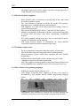
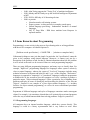


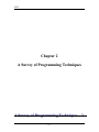

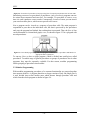

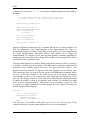
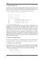
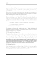
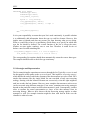


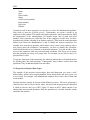
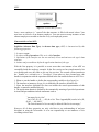
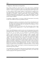


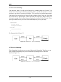


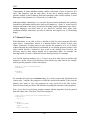


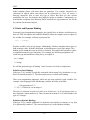
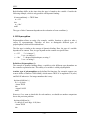


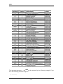


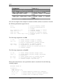

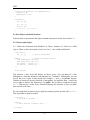

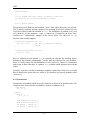
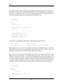
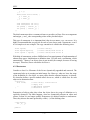

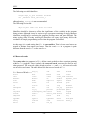
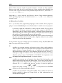
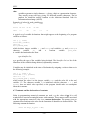

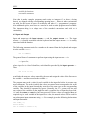


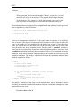
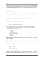

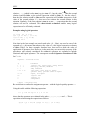
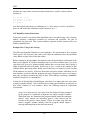
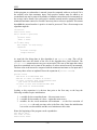
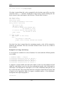


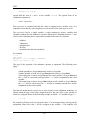
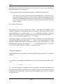
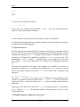
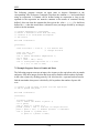
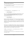


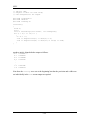

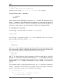


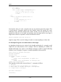
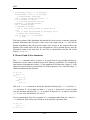


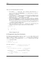
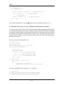

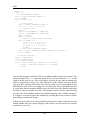


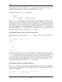
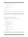

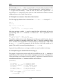
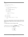
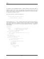


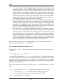
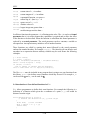
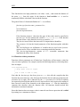

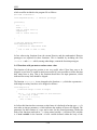
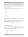
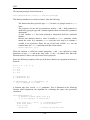
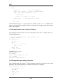

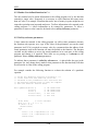
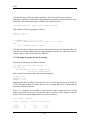
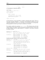
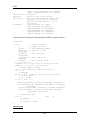
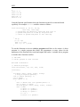


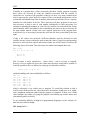
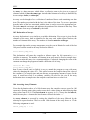
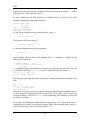

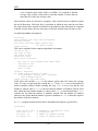
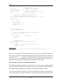
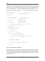
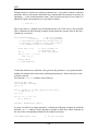
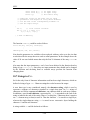


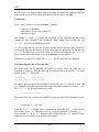
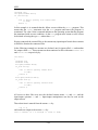
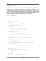


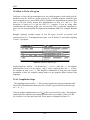
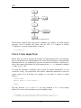
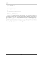







![Olympus µ[mju:]-mini DIGITAL](http://vs1.manualzilla.com/store/data/007181998_1-9144a7fcfac5b4a8090058e0c5c18757-150x150.png)