1
Jaguar User Manual
Jaguar 7.5
User Manual
Schrödinger Press
Jaguar User Manual Copyright © 2008 Schrödinger, LLC. All rights reserved.
While care has been taken in the preparation of this publication, Schrödinger
assumes no responsibility for errors or omissions, or for damages resulting from
the use of the information contained herein.
Canvas, CombiGlide, ConfGen, Epik, Glide, Impact, Jaguar, Liaison, LigPrep,
Maestro, Phase, Prime, PrimeX, QikProp, QikFit, QikSim, QSite, SiteMap, Strike, and
WaterMap are trademarks of Schrödinger, LLC. Schrödinger and MacroModel are
registered trademarks of Schrödinger, LLC. MCPRO is a trademark of William L.
Jorgensen. Desmond is a trademark of D. E. Shaw Research. Desmond is used with
the permission of D. E. Shaw Research. All rights reserved. This publication may
contain the trademarks of other companies.
Schrödinger software includes software and libraries provided by third parties. For
details of the copyrights, and terms and conditions associated with such included
third party software, see the Legal Notices for Third-Party Software in your product
installation at $SCHRODINGER/docs/html/third_party_legal.html (Linux OS) or
%SCHRODINGER%\docs\html\third_party_legal.html (Windows OS).
This publication may refer to other third party software not included in or with
Schrödinger software ("such other third party software"), and provide links to third
party Web sites ("linked sites"). References to such other third party software or
linked sites do not constitute an endorsement by Schrödinger, LLC. Use of such
other third party software and linked sites may be subject to third party license
agreements and fees. Schrödinger, LLC and its affiliates have no responsibility or
liability, directly or indirectly, for such other third party software and linked sites,
or for damage resulting from the use thereof. Any warranties that we make
regarding Schrödinger products and services do not apply to such other third party
software or linked sites, or to the interaction between, or interoperability of,
Schrödinger products and services and such other third party software.
Revision A, September 2008
Contents
Document Conventions ................................................................................................... xiii
Chapter 1: Introduction ....................................................................................................... 1
1.1 About This Manual .................................................................................................... 1
1.2 Running Schrödinger Software .............................................................................. 2
1.3 Citing Jaguar in Publications .................................................................................. 2
Chapter 2: Running Jaguar From Maestro ........................................................... 3
2.1 Sample Calculation ................................................................................................... 3
2.2 The Jaguar Panel ....................................................................................................... 6
2.3 The Edit Job Dialog Box .......................................................................................... 8
2.4 Molecular Structure Input ........................................................................................ 9
2.4.1 Cartesian Format for Geometry Input ............................................................... 10
2.4.2 Variables in Cartesian Input .............................................................................. 10
2.4.3 Constraining Cartesian Coordinates ................................................................. 11
2.4.4 Z-Matrix Format for Geometry Input ................................................................. 11
2.4.5 Variables and Dummy Atoms in Z-Matrix Input................................................. 13
2.4.6 Constraining Z-Matrix Bond Lengths or Angles ................................................ 14
2.4.7 Counterpoise Calculations ................................................................................ 14
2.4.8 Specifying Coordinates for Hessian Refinement............................................... 16
2.5 Reading Files ........................................................................................................... 17
2.6 Setting Charge and Multiplicity ............................................................................ 18
2.7 Cleaning up Molecular Geometries...................................................................... 18
2.7.1 Quick Geometry Optimization ........................................................................... 19
2.7.2 Symmetrization ................................................................................................. 19
2.8 Writing Files ............................................................................................................. 20
2.9 Running Jobs ........................................................................................................... 21
2.9.1 Output Handling ................................................................................................ 22
2.9.2 Job Submission Options ................................................................................... 23
2.9.3 Starting and Monitoring Jobs ............................................................................ 24
Jaguar 7.5 User Manual
iii
Contents
2.10 Running Jaguar Batch Jobs .............................................................................. 24
2.11 Output...................................................................................................................... 26
2.12 J2 Theory Calculations ........................................................................................ 27
2.13 Binding Energies of Hydrogen-Bonded Complexes ....................................... 27
Chapter 3: Options .............................................................................................................. 31
3.1 Molecule Settings .................................................................................................... 31
3.2 Basis Sets ................................................................................................................. 32
3.3 Density Functional Theory (DFT) Settings ......................................................... 37
3.4 Hartree-Fock and CIS Settings ............................................................................. 42
3.5 Local MP2 Settings ................................................................................................. 42
3.6 Generalized Valence Bond (GVB) Settings......................................................... 45
3.7 GVB-LMP2 Settings ................................................................................................ 45
3.8 SCF Settings ............................................................................................................ 47
3.8.1 Accuracy Level.................................................................................................. 47
3.8.2 Convergence Criteria ........................................................................................ 48
3.8.3 Convergence Methods ...................................................................................... 49
3.8.4 Orbital Treatment .............................................................................................. 50
3.9 Solvation Settings ................................................................................................... 51
3.9.1 Poisson-Boltzmann Solvation Model................................................................. 51
3.9.2 Solvation Model 6 ............................................................................................. 53
3.10 Properties ............................................................................................................... 55
3.10.1 Charges from Electrostatic Potential Fitting .................................................... 56
3.10.2 Mulliken Population Analysis........................................................................... 57
3.10.3 Multipole Moments.......................................................................................... 57
3.10.4 Natural Bond Orbital (NBO) Analysis.............................................................. 58
3.10.5 Polarizability and Hyperpolarizability .............................................................. 58
3.10.6 NMR Shielding Constants............................................................................... 59
3.10.7 Atomic Fukui Indices....................................................................................... 60
3.10.8 Molecular Properties from SM6 Calculations.................................................. 60
iv
Jaguar 7.5 User Manual
Contents
3.11 Frequencies and Related Properties ................................................................. 61
3.11.1 Frequencies .................................................................................................... 61
3.11.2 Atomic Masses................................................................................................ 61
3.11.3 Scaling of Frequencies.................................................................................... 62
3.11.4 Animation of Frequencies ............................................................................... 64
3.11.5 Infrared Intensities .......................................................................................... 65
3.11.6 Thermochemical Properties............................................................................ 65
3.12 Surfaces .................................................................................................................. 66
Chapter 4: Optimizations and Scans ...................................................................... 71
4.1 Geometry Optimization: The Basics .................................................................... 71
4.1.1 SCF and Geometry Convergence..................................................................... 72
4.1.2 The Initial Hessian ............................................................................................ 73
4.1.3 Coordinate Systems.......................................................................................... 74
4.2 Constraining Coordinates...................................................................................... 74
4.2.1 Freezing Specific Coordinates .......................................................................... 75
4.2.2 Applying Harmonic Constraints......................................................................... 76
4.2.3 Applying Constraints by Using Variables .......................................................... 77
4.2.4 Applying Dynamic Constraints .......................................................................... 78
4.3 Transition-State Optimizations ............................................................................. 78
4.3.1 Transition-State Search Method........................................................................ 79
4.3.2 Specifying Structures for the Reaction.............................................................. 80
4.3.3 Searching Along a Particular Hessian Eigenvector........................................... 81
4.3.4 Refinement of the Initial Hessian ...................................................................... 82
4.4 Geometry Scans ...................................................................................................... 84
4.4.1 Setting up Scans in Maestro ............................................................................. 84
4.4.2 Setting up Input Files for Scans ........................................................................ 86
4.4.3 Constraining Coordinates for Torsional Scans .................................................. 87
4.4.4 Restarting Scans .............................................................................................. 88
4.4.5 Scan Results..................................................................................................... 88
4.5 Intrinsic Reaction Coordinate Calculations ....................................................... 88
Jaguar 7.5 User Manual
v
Contents
Chapter 5: Output ................................................................................................................. 93
5.1 Summarizing Jaguar Results ................................................................................ 93
5.1.1 Reporting Final Results From One or More Jobs ............................................. 96
5.1.2 Reporting Intermediate Results ........................................................................ 97
5.1.3 Reporting Results for Each Atom...................................................................... 98
5.2 Output From a Standard HF Calculation ............................................................. 98
5.3 Output File Content for Various Calculation Types ........................................ 102
5.3.1 DFT ................................................................................................................. 103
5.3.2 LMP2............................................................................................................... 103
5.3.3 GVB ................................................................................................................ 104
5.3.4 Geometry or Transition-State Optimization ..................................................... 105
5.3.5 Solvation ......................................................................................................... 108
5.3.5.1 Output from a PBF Calculation ............................................................. 108
5.3.5.2 Output from an SM6 Calculation ........................................................... 112
5.3.6 Geometry Optimization in Solution ................................................................. 115
5.3.7 Properties ....................................................................................................... 115
5.3.7.1 Multipole Moments and Charge Fitting .................................................. 115
5.3.7.2 Polarizabilities and Hyperpolarizabilities................................................ 117
5.3.7.3 Electron Density .................................................................................. 119
5.3.7.4 Mulliken Populations ............................................................................ 119
5.3.7.5 Atomic Fukui Indices ............................................................................ 120
5.3.7.6 NBO Calculations ................................................................................ 122
5.3.8 Frequency, IR Intensity, and Thermochemistry Output ................................... 122
5.3.9 CIS Calculations ............................................................................................. 124
5.3.10 Basis Set....................................................................................................... 125
5.3.11 Methods ........................................................................................................ 128
5.4 Options for Extra Output...................................................................................... 128
5.5 File Output Options ............................................................................................... 132
5.6 Output Options for Orbitals ................................................................................. 133
5.7 The Log File ............................................................................................................ 136
vi
Jaguar 7.5 User Manual
Contents
Chapter 6: Using Jaguar................................................................................................ 139
6.1 Choosing an Initial Guess ................................................................................... 139
6.1.1 Overview ......................................................................................................... 139
6.1.2 GVB Initial Guess............................................................................................ 140
6.1.3 Initial Guess for Molecules Containing Transition Metals................................ 141
6.2 SCF Convergence.................................................................................................. 142
6.3 Geometry Optimization ........................................................................................ 143
6.4 Setting Up GVB Calculations .............................................................................. 144
6.5 Restarting Jobs and Using Previous Results .................................................. 144
6.6 Conformational Searches .................................................................................... 146
6.7 Generating Input Files for GAUSSIAN .................................................................. 147
Chapter 7: Theory .............................................................................................................. 149
7.1 The Pseudospectral Method ............................................................................... 149
7.2 Pseudospectral Implementation of the GVB Method ..................................... 151
7.3 GVB-RCI Wave Functions .................................................................................... 155
7.4 Pseudospectral Local MP2 Techniques ............................................................ 157
7.5 Density Functional Theory .................................................................................. 160
Chapter 8: The Jaguar Input File ............................................................................. 163
8.1 General Description of the Input File................................................................. 163
8.1.1 Input File Format............................................................................................. 163
8.1.2 Sections Describing the Molecule and Calculation ......................................... 164
8.2 The zmat, zmat2, and zmat3 Sections ............................................................... 166
8.3 The zvar, zvar2, and zvar3 Sections ................................................................... 168
8.4 The coord and connect Sections ....................................................................... 169
8.4.1 Constrained Coordinates ................................................................................ 169
8.4.2 Specifying Bonds for Internal Coordinates with a connect Section................. 171
Jaguar 7.5 User Manual
vii
Contents
8.5 The gen Section ..................................................................................................... 171
8.5.1 Units Keywords ............................................................................................... 172
8.5.2 Covalent Bonding Keyword ............................................................................. 172
8.5.3 Molecular State Keywords (Charge and Multiplicity)....................................... 173
8.5.4 Atomic Mass Keyword..................................................................................... 173
8.5.5 Symmetry-Related Keywords.......................................................................... 173
8.5.6 GVB and Lewis Dot Structure Keywords ........................................................ 174
8.5.7 LMP2 Keywords .............................................................................................. 175
8.5.8 DFT Keywords ................................................................................................ 177
8.5.9 CIS and TDDFT Keywords.............................................................................. 185
8.5.10 Geometry Optimization and Transition-State Keywords................................ 185
8.5.11 Geometry Scan Keywords ............................................................................ 191
8.5.12 Intrinsic Reaction Coordinate (IRC) Keywords.............................................. 192
8.5.13 Solvation Keywords....................................................................................... 194
8.5.14 Properties Keywords ..................................................................................... 195
8.5.15 Frequency-Related Keywords ....................................................................... 199
8.5.16 Basis Set Keywords ...................................................................................... 200
8.5.17 Keywords for SCF Methods .......................................................................... 201
8.5.18 Initial Guess Keywords.................................................................................. 206
8.5.19 Localization Keywords .................................................................................. 208
8.5.20 File Format Conversion Keywords ................................................................ 209
8.5.21 Standard Output Keywords ........................................................................... 212
8.5.22 File Output Keywords.................................................................................... 214
8.5.23 Output Keywords for Each Iteration .............................................................. 215
8.5.24 Orbital Output Keywords ............................................................................... 216
8.5.25 Grid and Dealiasing Function Keywords ....................................................... 218
8.5.26 Memory Use Keywords ................................................................................. 220
8.5.27 Plotting Keywords ......................................................................................... 222
8.6 The gvb Section ..................................................................................................... 225
8.7 The lmp2 Section ................................................................................................... 226
8.8 The atomic Section ............................................................................................... 227
8.8.1 General Format of the atomic Section ........................................................... 227
8.8.2 Keywords That Specify Physical Properties.................................................... 229
viii
Jaguar 7.5 User Manual
Contents
8.8.3 Basis, Grid, Dealiasing Function, and Charge Usage for Individual Atoms .... 230
8.8.4 Defining Fragments......................................................................................... 235
8.9 The hess Section ................................................................................................... 236
8.10 The guess and guess_basis Sections............................................................. 237
8.11 The pointch Section ............................................................................................ 239
8.12 The efields Section ............................................................................................. 239
8.13 The ham Section.................................................................................................. 240
8.14 The orbman Section ........................................................................................... 240
8.15 The echo Section................................................................................................. 241
8.16 The path Section ................................................................................................. 241
8.17 NBO Sections ....................................................................................................... 244
Chapter 9: Other Jaguar Files ................................................................................... 245
9.1 The Basis Set File.................................................................................................. 245
9.1.1 Basis Set Format ............................................................................................ 245
9.1.2 Effective Core Potential Format ...................................................................... 247
9.1.3 Customizing Basis Sets .................................................................................. 249
9.2 The Initial Guess Data File ................................................................................... 250
9.3 The Dealiasing Function File............................................................................... 252
9.3.1 File Format and Description............................................................................ 253
9.3.2 Sample File ..................................................................................................... 255
9.4 The Grid File ........................................................................................................... 257
9.4.1 File Format and Description............................................................................ 257
9.5 The Cutoff File........................................................................................................ 260
9.6 The Lewis File ........................................................................................................ 262
9.6.1 Describing Bonding Types in the Lewis File.................................................... 264
9.6.2 Describing Hybridization Types in the Lewis File ............................................ 265
9.6.3 Setting van der Waals Radii From Lewis File Data ......................................... 267
9.6.4 Default Behavior for Setting Radii ................................................................... 270
Jaguar 7.5 User Manual
ix
Contents
Chapter 10: Running Jobs ........................................................................................... 273
10.1 The jaguar Command ......................................................................................... 273
10.1.1 Selecting an Execution Host ......................................................................... 275
10.1.2 Selecting Particular Jaguar Executables....................................................... 276
10.1.3 Running a Jaguar Job From the Command Line .......................................... 276
10.1.4 Killing a Jaguar Job....................................................................................... 278
10.1.5 Converting File Formats................................................................................ 279
10.2 Running Multiple Jobs: jaguar batch .............................................................. 282
10.2.1 Batch Input File Format................................................................................. 282
10.2.2 Running jaguar batch.................................................................................... 286
10.2.3 Batch Input File Examples ............................................................................ 287
10.2.3.1 Pipelined Jobs ................................................................................... 288
10.2.3.2 Running Jobs from Input in a Specified Directory ................................ 288
10.2.4 Using Python Scripts with jaguar batch ........................................................ 289
10.2.4.1 counterpoise.py ................................................................................. 289
10.2.4.2 hydrogen_bond.py ............................................................................. 290
10.2.4.3 distributed_scan.py ............................................................................ 291
Chapter 11: Troubleshooting....................................................................................... 293
11.1 Problems Getting Started .................................................................................. 293
11.1.1 The SCHRODINGER Environment Variable................................................. 293
11.1.2 Including the jaguar Command in Your Path................................................. 294
11.1.3 Problems Starting Maestro ........................................................................... 295
11.1.4 Problems Related to Your Temporary Directory............................................ 296
11.1.5 Problems Running Jaguar Calculations on Other Nodes.............................. 297
11.2 Other Problems.................................................................................................... 298
Chapter 12: Parallel Jaguar ......................................................................................... 301
12.1 General Installation Information ....................................................................... 301
12.2 Linux-x86 Installation ......................................................................................... 302
12.2.1 Configuration With a Queueing System........................................................ 304
12.2.2 Configuration Without a Queueing System................................................... 304
x
Jaguar 7.5 User Manual
Contents
12.2.3 Testing and Troubleshooting Parallel Job Problems...................................... 305
12.3 SGI Linux-ia64 (Altix) Installations................................................................... 306
12.4 Linux-ia64 (non-SGI) Installations.................................................................... 306
12.5 Building Jaguar’s MPI Compatibility Libraries .............................................. 307
Chapter 13: The pKa Prediction Module ............................................................. 309
13.1 Theory of pKa Calculation ................................................................................. 310
13.1.1 Ab initio Quantum Chemical Calculation of pKa Values ................................ 310
13.1.2 Empirical Corrections.................................................................................... 312
13.2 Predicting pKa Values in Complex Systems ................................................. 313
13.2.1 Conformational Flexibility .............................................................................. 313
13.2.2 Equivalent Sites ............................................................................................ 314
13.2.3 Multiple Protonation Sites ............................................................................. 315
13.3 Training Set Results............................................................................................ 315
13.4 Running pKa Calculations ................................................................................. 317
13.4.1 Activating the pKa Module ............................................................................. 317
13.4.2 Running pKa Calculations from Maestro ....................................................... 317
13.4.3 Jaguar Input Files for pKa Calculations ......................................................... 320
13.4.4 Running pKa Calculations from the Command Line...................................... 320
13.4.5 Monitoring pKa Calculations.......................................................................... 322
13.4.6 Choice of Initial Geometry ............................................................................ 322
13.4.7 Recalculating pKa Values with New Parameters .......................................... 323
13.5 Developing Your Own pKa Correction Parameters ....................................... 324
Getting Help ........................................................................................................................... 327
References .............................................................................................................................. 331
Index ............................................................................................................................................ 341
Keyword Index ...................................................................................................................... 355
Jaguar 7.5 User Manual
xi
xii
Jaguar 7.5 User Manual
Document Conventions
In addition to the use of italics for names of documents, the font conventions that are used in
this document are summarized in the table below.
Font
Example
Use
Sans serif
Project Table
Names of GUI features, such as panels, menus,
menu items, buttons, and labels
Monospace
$SCHRODINGER/maestro
File names, directory names, commands, environment variables, and screen output
Italic
filename
Text that the user must replace with a value
Sans serif
uppercase
CTRL+H
Keyboard keys
Links to other locations in the current document or to other PDF documents are colored like
this: Document Conventions.
In descriptions of command syntax, the following UNIX conventions are used: braces { }
enclose a choice of required items, square brackets [ ] enclose optional items, and the bar
symbol | separates items in a list from which one item must be chosen. Lines of command
syntax that wrap should be interpreted as a single command.
File name, path, and environment variable syntax is generally given with the UNIX conventions. To obtain the Windows conventions, replace the forward slash / with the backslash \ in
path or directory names, and replace the $ at the beginning of an environment variable with a
% at each end. For example, $SCHRODINGER/maestro becomes %SCHRODINGER%\maestro.
In this document, to type text means to type the required text in the specified location, and to
enter text means to type the required text, then press the ENTER key.
References to literature sources are given in square brackets, like this: [10].
Jaguar 7.5 User Manual
xiii
xiv
Jaguar 7.5 User Manual
Jaguar User Manual
Chapter 1
Chapter 1:
Introduction
1.1
About This Manual
The Jaguar User Manual is intended to help you perform ab initio calculations for a variety of
methods, parameters, and calculated properties. Jaguar can be run from the command line or
from the Maestro graphical user interface (GUI). Online help is available in the GUI, although
the information in this manual is generally more comprehensive.
Chapter 2 contains information you will need to run Jaguar, including information about using
the GUI, geometry input formats, specifying file names for input and output, displaying molecular geometries, symmetrizing geometries, and setting run-time parameters, such as the
machine that will perform the calculation. We suggest you start by trying the sample calculation in Section 2.1. If the calculation runs successfully, you can proceed to the rest of the
chapter to learn how to input molecular structures and run jobs. If you have problems starting
Maestro or running the sample calculation, see the troubleshooting information in Chapter 11.
Chapters 3 and 4 describe the available calculation options, which allow you to specify which
properties you want the program to calculate and which methods you want it to use. Chapter 3
includes information on using generalized valence bond (GVB), restricted configuration interaction (RCI), Møller-Plesset second-order perturbation theory, and density functional theory
(DFT) techniques; calculating solvation energies, vibrational frequencies, hyperpolarizabilities, multipole moments, and other properties; fitting charges; specifying basis sets; and
various other options. Chapter 4 describes optimizations of the molecular structure, transitionstate searches, and geometry scans.
Chapter 5 describes how to summarize Jaguar output and the output or printing options available from the GUI. The output file containing the primary Jaguar output is first described for
cases where no Output options have been selected. Next, the output given when various Output
settings are turned on is explained. Finally, the log file is described.
Chapter 6 contains tips and suggestions for using Jaguar. The chapter includes some general
tips for different sorts of calculations: a description of how to restart calculations, how to incorporate results from previous runs, and some tips on using both Jaguar and GAUSSIAN.
Chapter 7 describes some of the theory behind the pseudospectral method and the electron
correlation methods used in Jaguar. This chapter includes information on pseudospectral
implementations of GVB and local MP2 techniques, and a brief description of density functional theory.
Jaguar 7.5 User Manual
1
Chapter 1: Introduction
Chapter 8 describes the Jaguar input file in detail. You may find this chapter especially useful if
you want to run some jobs without using the GUI. Chapter 9 describes other Jaguar files that
are necessary for calculations. You may skip Chapter 8 and Chapter 9 if you want to run all
jobs from the GUI, but you might want to skim them anyway to find out more about Jaguar and
the methods it uses.
Chapter 10 provides information on submitting jobs from the command line, and running
multiple Jaguar jobs using batch scripts.
Chapter 11 contains troubleshooting hints concerning various problems you might encounter,
especially when first setting up Jaguar on your system. Chapter 12 contains information on
running calculations on parallel computers. Chapter 13 describes the pKa calculation module.
1.2
Running Schrödinger Software
To run any Schrödinger program on a Unix platform, or start a Schrödinger job on a remote
host from a Unix platform, you must first set the SCHRODINGER environment variable to the
installation directory for your Schrödinger software. To set this variable, enter the following
command at a shell prompt:
csh/tcsh:
setenv SCHRODINGER installation-directory
bash/ksh:
export SCHRODINGER=installation-directory
Once you have set the SCHRODINGER environment variable, you can start Maestro with the
following command:
$SCHRODINGER/maestro &
It is usually a good idea to change to the desired working directory before starting Maestro.
This directory then becomes Maestro’s working directory. For more information on starting
Maestro, including starting Maestro on a Windows platform, see Section 2.1 of the Maestro
User Manual.
1.3
Citing Jaguar in Publications
The use of this product should be acknowledged in publications as:
Jaguar, version 7.5, Schrödinger, LLC, New York, NY, 2008.
2
Jaguar 7.5 User Manual
Jaguar User Manual
Chapter 2
Chapter 2:
Running Jaguar From Maestro
The Maestro interface to Jaguar can simplify the preparation and submission of jobs. You can
run Maestro on one machine, display it to another, and start a Jaguar calculation on yet another
machine. The main part of the interface is the Jaguar panel, which you use to prepare job input.
Without the Jaguar panel, you would have to create input files with particular formats in order
to run Jaguar. Maestro creates these input files for you, based on information you provide, and
submits the job. This frees you from learning the input format and program sequences, and
instead allows you to concentrate on the science.
Try the sample calculation in Section 2.1 to get some experience running Jaguar and to make
sure your system is set up properly. If you have problems starting or using Maestro or
performing the calculation, you may be able to solve them using the troubleshooting suggestions in Chapter 11. If any problems persist, contact your system manager or Schrödinger.
The rest of this chapter describes the basics of running Jaguar from Maestro, including
entering a geometry and submitting a job. Jaguar has a wide range of options for different
kinds of calculations. Setting these from Maestro is described in Chapter 3. Jaguar can perform
many kinds of calculations, such as geometry optimizations, transition-state searches, and
various coordinate scans. Setting up these calculations is described in Chapter 4. Jaguar also
provides special capabilities for pKa prediction and accurate calculations with J2 theory. J2
theory calculations are described in this chapter; pKa calculations are described in Chapter 13.
The footnotes describe Jaguar input file keywords and sections that correspond to particular
GUI settings. If you are working from Maestro, you can ignore these footnotes, but you may
later find them helpful if you decide to use input files to submit jobs without using Maestro, or
if you want to edit keywords directly using the Edit Job dialog box.
2.1
Sample Calculation
This section provides instructions for running a sample calculation on the water molecule. The
sample calculation runs only if Jaguar has been correctly installed. If the calculation does not
run, try the suggestions in Chapter 11, or see your system manager or the person who installed
Jaguar at your site. Contact Schrödinger if you cannot resolve the installation problems.
First, log on to a machine where the Maestro and Jaguar software is installed. Change to the
directory where you want the Jaguar output files for the sample job to be written, then start
Maestro by entering the command
Jaguar 7.5 User Manual
3
Chapter 2: Running Jaguar From Maestro
$SCHRODINGER/maestro &
If $SCHRODINGER is in your PATH environment variable, you can simply type maestro. Once
Maestro is running, choose Single Point Energy from the Jaguar submenu of the Applications
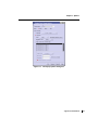
menu to open the Jaguar panel for a single point energy calculation (see Figure 2.1 on page 7).
The next step is to enter a molecular geometry (structure). You can enter the structure by hand
or read it from a file.
To enter the structure by hand, you can use the Edit Job window. Click the Edit button, select
the Structure option, then click in the text area and type the following lines:
O
H1
H2
0.0
0.753108
-0.753108
0.0
0.0
0.0
-0.1135016
0.4540064
0.4540064
The labels begin with element symbols, O and H. The numerals 1 and 2 appended to the
hydrogen labels distinguish between the atoms. The next three numbers on each line give the x,
y, and z Cartesian coordinates of the atoms in the geometry, in angstroms. The number of
spaces you type does not matter, as long as you use at least one space to separate different
items. When you finish entering the water geometry, click OK.
To read in the structure, click Read, then navigate to the following directory:
$SCHRODINGER/jaguar-vversion/samples
where version is the 5-digit version number of your Jaguar software. Select H2O.in from the
file list, and click OK.
Whichever method of entry you chose, the molecular structure should now be shown in the
Workspace. If you entered the geometry by hand, the structure is a scratch entry. You can run
the job with a scratch entry, but the results will not be incorporated into the Project Table
unless you make it a named entry. To do so, click the Create entry from Workspace button in
the toolbar, and name the entry H2O.
When you finish setting up your calculation, click the Start button. The Start dialog box is
displayed (see Figure 2.5 on page 22). In this dialog box you can make settings for running the
job. In the Output section, you can select an option for incorporation of results. Choose
Replace existing entries.
In the Job section, you can provide a job name, select the execution host, the number of
processors, and the scratch directory. The entry name, H2O, appears in the Name text box. The
names of the input, output, and log files for your job depend on the name you provide: the
4
Jaguar 7.5 User Manual
Chapter 2: Running Jaguar From Maestro
Jaguar input file is named jobname.in, the output file is named jobname.out, and the log file
is named jobname.log, where jobname is the text that appears in the Name text box.
The default execution host (the machine that the job will run on) is selected in the Host option
menu. This default is localhost, which means the machine on which Maestro is running. The
host name is followed by the number of available processors in parentheses. If Jaguar is
installed on more than one machine at your site, you can change the choice of execution host
by selecting another host from the option menu. The Scratch directory option menu displays
the directory on the execution host that will be used during the calculation to store temporary
files. You should check that the directory already exists on the execution host. If it does not
exist, you should create it.
You should not need to change any other settings. Click the Start button to start the job. After
you start the job, the Monitor panel is displayed. This panel is automatically updated to show
the progress of your job. As each separate program in the Jaguar code finishes running, its
completion is noted in the log text area. When the program scf is running, the Monitor panel
displays the energy and other data of each iteration. See Section 5.7 on page 136 on the log file
for more information on this data. You can close the Monitor panel by clicking the Close
button. If you want to reopen it later, you can do so by choosing Monitor Jobs from the Applications menu in the main window.
When the job finishes, its output file is copied to the directory from which you started Maestro.
The output file ends with the extension .out. For instance, if you entered the job name h2o, the
output file would be h2o.out.
If you want to exit Maestro, choose Quit from the Maestro menu in the Maestro main window.
The Quit dialog box permits you to save a log file of the Maestro session. For this exercise,
choose Quit, do not save log file. A warning dialog box is displayed, which permits you to save
the Maestro scratch project. For this exercise, choose Discard.
To check that the job ran correctly, change to the directory where the output file was stored and
enter the following command:
diff -w jobname.out $SCHRODINGER/jaguar-vversion/samples/H2O.out
If there is no output from this command, the job ran correctly. If there is output, examine the
differences between the two files to see if the differences are significant.
If you are satisfied with the results of this sample run, continue this chapter to learn more about
using Maestro. If you were unable to run the sample calculation, see the troubleshooting
suggestions in Chapter 11.
Jaguar 7.5 User Manual
5
Chapter 2: Running Jaguar From Maestro
2.2
The Jaguar Panel
The Jaguar panel is the main interface between Maestro and Jaguar. In this panel, you can set
up input files for a range of Jaguar jobs, and start the jobs. To open the panel, choose the task or
calculation type from the Jaguar submenu of the Applications menu in the main window. The
available tasks are:
•
•
•
•
•
•
•
Single Point Energy
Optimization
Relaxed Coordinate Scan
Rigid Coordinate Scan
Transition State Search
Reaction Coordinate
Initial Guess Only
Below these tasks in the menu are several calculation types that are run as Jaguar batch jobs:
•
•
•
•
pKa
Hydrogen Bond
Counterpoise
J2
The input for these calculations is described in this chapter and Chapter 13.
Most of the Jaguar panel is occupied by a set of tabs in which you can make settings for jobs.
These tabs are described in Chapter 3 and Chapter 4. At the top of the panel is a section for
selecting the source of job input. The Use structures from option menu has three choices:
• Workspace (included entries)—the structures that are displayed in the Workspace.
• Selected entries—the structures that are selected in the Project Table. These need not be
the same as the included entries.
• Selected structure files—the structures that are in the files listed in the Files text box. You
can navigate to the desired files using the Browse button. When you click OK in the file
selector that is displayed, the file name is added to the list in the Files text box.
If you select either of the first two sources of job input, the results of the calculations can be
incorporated into the Maestro project. If you run from structure files, the results cannot be
incorporated automatically.
You can select multiple structures as input for many kinds of Jaguar calculations. When you
do, Maestro creates a Jaguar batch script that runs the calculation for each structure independently. These independent calculations can be run across multiple processors. For more information, see Section 2.9 on page 21.
6
Jaguar 7.5 User Manual
Chapter 2: Running Jaguar From Maestro
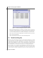
Figure 2.1. The Jaguar panel.
Below the tabs is the Job text box, in which a summary of the calculation type is displayed, and
below this text box is a row of buttons:
• Start—Opens a dialog box in which you can make selections for running the job and
incorporating the output, and then start the job. See Section 2.9 on page 21.
• Read—Opens a file browser for selecting a Jaguar input file to read in. See Section 2.5 on
page 17.
• Write—Opens a file browser for writing the current geometry and settings in the Jaguar
panel as an input file or for writing the current settings as a batch script.
Jaguar 7.5 User Manual
7
Chapter 2: Running Jaguar From Maestro
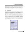
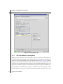
Figure 2.2. The Edit Job dialog box with Structure selected.
• Edit—Opens the Edit Job dialog box, in which you can edit the contents of the input file.
Any changes you make in this dialog box are reflected in the settings in the Jaguar panel.
You can also add keywords that are not available as GUI settings—see the next section.
• Reset—Resets all the settings in the Jaguar panel to the default state for the selected task.
• Close—Closes the Jaguar panel.
• Help—Opens the help viewer at the topic for the currently displayed tab.
2.3
The Edit Job Dialog Box
While most of the common settings for Jaguar jobs can be made in the Jaguar panel, you might
need to make changes to the settings, add keywords to the input file for options that are not
available from the Jaguar panel, or make changes to the geometry. You can make these
changes in the Edit Job dialog box, which you open by clicking Edit in the Jaguar panel. Apart
from standard editing tools, this dialog box has special tools for editing Jaguar input files.
The basic editing tools are contained in the File and Edit menus. The File menu allows you to
save the current state of the input file to disk (Write), and to cancel all your changes without
closing the dialog box (Revert). The Edit menu provides Cut, Copy, and Paste options for
8
Jaguar 7.5 User Manual
Chapter 2: Running Jaguar From Maestro
cutting and pasting within Maestro, but you cannot use these to copy text from another application. To copy and paste text from another application (or from Maestro), highlight the text, then
middle-click where you want the text to be pasted. The text in the paste buffer is saved when
you close the dialog box, so you can copy text between input files.
The Edit Job dialog box has two editing modes: Input File and Structure. By default, the entire
input file is available for editing. In Structure mode, only the geometry is displayed, and a
Structure menu is added to the menu bar. If you are editing geometries for a transition state
search or an IRC scan, all three geometries can be edited. The editing area has tabs for each of
these geometries, labeled Reactant, Product, and Transition State.
The Structure menu provides options for modifying the geometry input. The Convert to
Z-matrix and Convert to Cartesians options switch between Z-matrix format and Cartesian
format. The option Assign Unique Atom Labels converts all atom labels to the form El#, where
El is the standard element symbol (Fe for iron, for instance) and # is the atom number in the
input list (1 for the first atom, 2 for the second, and so on). This option guarantees that all
atoms have unique atom labels, which is required by Jaguar. Unique atom labels are assigned
automatically if Jaguar detects any ambiguity in the labels. You can display the atom labels in
the Workspace by choosing View Atom Labels. The remaining option on the Structure menu is
useful for transition state searches, but not for other Jaguar jobs. This option is described in
Section 4.3 on page 78.
The changes you make are automatically saved in the Maestro project, and are reflected in the
panel settings. You can view the changes to the geometry in the Workspace by clicking
Preview.
Note:
2.4
Counterpoise atoms, constraints and coordinates for Hessian refinement should not be
added in this dialog box: they are removed when you close the dialog box.
Molecular Structure Input
After you start Maestro, the first task for setting up any Jaguar calculation is to enter a molecular structure (geometry).1 You can create a structure using Maestro’s Build panel, you can use
the Jaguar panel to read in a file as described in Section 2.5 on page 17, or you can enter and
edit the geometry yourself, in Cartesian (x, y, z) coordinates or in Z-matrix format, using the
Edit Job dialog box. This section describes the input formats for Cartesian and Z-matrix geometries. The geometry input is used to set constraints of bond lengths or angles for geometry
optimization and to specify atoms for a counterpoise calculation. These aspects of geometry
input are explained in this section as well.
1.
The geometry input is in the zmat and zvar sections of the input file.
Jaguar 7.5 User Manual
9
Chapter 2: Running Jaguar From Maestro
The geometries that you enter are displayed in the Workspace, in which you can rotate and
translate the structure, change the geometry, display in various representations, and perform
many other tasks. For information on Maestro, see the Maestro User Manual.
2.4.1
Cartesian Format for Geometry Input
The Cartesian geometry input format can consist of a simple list of atom labels and the atomic
coordinates in angstroms in Cartesian (x, y, z) form. For example, the input
O
H1
H2
0.000000
0.000000
0.000000
0.000000
0.753108
-0.753108
-0.113502
0.454006
0.454006
describes a water molecule. Each atomic label must start with the one- or two-letter element
symbol, and may be followed by additional characters, as long as the atomic label has eight or
fewer characters and the atomic symbol remains clear. For example, HE5 would be interpreted
as helium atom 5, not hydrogen atom E5. The atom label is case-insensitive. The coordinates
may be specified in any valid C format, but each line of the geometry input should contain no
more than 80 characters.
2.4.2
Variables in Cartesian Input
Coordinates can also be specified as variables, whose values are set below the list of atomic
coordinates. This makes it easier to enter equal values and also makes it possible to keep
several atoms within the same plane during a geometry optimization.
To use variables, type the variable name (zcoor, for instance) where you would normally type
the corresponding numerical value for each relevant coordinate. You can prefix any variable
with a + or – sign. When you have entered the full geometry, add one or more lines setting the
variables. For instance, the Cartesian input
O
0.000000
H1 0.000000
H2 0.000000
ycoor=0.753108
0.000000 -0.113502
ycoor
zcoor
-ycoor
zcoor
zcoor=0.454006
describes the same water coordinates as the previous Cartesian input example. If you
performed a geometry optimization using this input structure, its ycoor and zcoor values
might change, but their values for one hydrogen atom would always be the same as those for
the other hydrogen atom, so the molecule would retain C2v symmetry.
The variable settings can also be separated from the coordinates by a line containing the text
Z-variables. For instance, the following input is equivalent to the previous example:
O
10
0.000000
0.000000
Jaguar 7.5 User Manual
-0.113502
Chapter 2: Running Jaguar From Maestro
H1 0.000000
H2 0.000000
Z-variables
ycoor=0.753108
zcoor=0.454006
ycoor
-ycoor
zcoor
zcoor
Note that if Cartesian input with variables is used for an optimization, Jaguar performs the
optimization using Cartesian coordinates instead of generating redundant internal coordinates,
and the optimization will not make use of molecular symmetry.
2.4.3
Constraining Cartesian Coordinates
As described in the previous section, you can force Cartesian coordinates to remain the same
as each other during an optimization by using variables. You can also specify Cartesian coordinates that should be frozen during a geometry optimization by adding a “#” sign after the coordinate values. For example, if you add constraints to the zcoor variables in the water input
example, as listed below,
O
0.000000
H1 0.000000
H2 0.000000
ycoor=0.753108
0.000000 -0.113502
ycoor
zcoor#
-ycoor
zcoor#
zcoor=0.454006
and perform a geometry optimization on this molecule, the H atoms would be allowed to move
only within the xy plane in which they started.
If frozen Cartesian coordinates are included in the input for an optimization, Jaguar uses Cartesian coordinates for the optimization rather than generating redundant internal coordinates, and
the optimization does not make use of molecular symmetry.
2.4.4
Z-Matrix Format for Geometry Input
Like Cartesian geometries, Z-matrix-format geometries also specify atoms by atom labels that
begin with the one- or two-letter element symbol. The atom label is case-insensitive. The
element symbol may be followed by additional characters, as long as the atom label has eight
or fewer characters and the element symbol is still clear.
The first line of the Z-matrix should contain only one item: the atom label for the first atom.
For example,
N1
This atom is placed at the origin. The second line contains the atom label for atom 2, the identifier of atom 1, and the distance between atoms 1 and 2. Identifiers can either be atom labels or
atom numbers (the position in the list: 1 for the first atom, 5 for the fifth atom listed, and so
Jaguar 7.5 User Manual
11
Chapter 2: Running Jaguar From Maestro
on). In this example, the identifier for the first atom could be either “N1” or “1.” The second
atom is placed along the positive z-axis. For example,
N1
C2
N1
1.4589
places the carbon atom (C2) at (0.0, 0.0, 1.4589) in Cartesian coordinates. Distances between
atoms must be positive.
The third line is made up of five items: the atom label for atom 3, the identifier of one of the
previous atoms, the distance between this atom and atom 3, the identifier of the other previous
atom, and the angle defined by the three atoms. In this example,
N1
C2
C3
N1
C2
1.4589
1.5203
N1
115.32
the final line states that atoms C3 and C2 are separated by 1.5203 Å and that the C3–C2–N1
bond angle is 115.32°. The bond angle must be between 0° and 180°, inclusive. The third atom
(C3 in this case) is placed in the xz plane (positive x).
The fourth line contains seven items: the atom label for atom 4, an atom identifier, the distance
between this atom and atom 4, a second atom identifier, the angle defined by these three atoms,
a third atom identifier, and a torsional angle. In this example,
N1
C2
C3
O4
N1
C2
C3
1.4589
1.5203
1.2036
N1
C2
115.32
126.28
N1
150.0
the last line states that atoms O4 and C3 are 1.2036 units apart, that the O4–C3–C2 bond angle
is 126.28°, and that the torsional angle defined by O4–C3–C2–N1 is 150.0°. This information
is sufficient to uniquely determine a position for O4. If the first three atoms in the torsional
angle definition were collinear or very nearly collinear, O4’s position would be poorly defined.
You should avoid defining torsional angles relative to three collinear (or nearly collinear)
angles. In such a case you should use dummy atoms to define the torsional angle (see
Section 2.4.5 on page 13).
The torsional angle is the angle between the plane formed by the first three atoms (in this case
N1–C2–C3) and the plane formed by the last three atoms (in this case C2–C3–O4). Looking
from the second to the third atom (C2 to C3), the sign of the angle is positive if the angle is
traced in a clockwise direction from the first plane to the second plane, and negative if the
angle is traced counterclockwise.
An alternative for specifying the fourth atom’s position is to use a second bond angle instead of
a torsional angle. To specify another bond angle, add 1 or −1 to the end of the line. The second
12
Jaguar 7.5 User Manual
Chapter 2: Running Jaguar From Maestro
bond angle is the angle between the first, second, and fourth atoms (in the example above, the
O4–C3–N1 angle). Since there are two possible positions for the atom which meet the angle
specifications, the position is defined by the scalar triple product r12⋅ (r23 × r24), where rij = ri −
rj is the vector pointing from atom j to atom i. If this product is positive, the value at the end of
the line should be 1. If it is negative, the value should be −1. You should use torsional angles
instead of second bond angles if you want to perform a constrained geometry optimization,
however, since Jaguar cannot interpret any constraints on bond lengths or angles for geometries containing second bond angles.
All additional lines of the Z-matrix should have the same form as the fourth line. The complete
Z-matrix for the example molecule (the 150˚ conformation of glycine) is
N1
C2
C3
O4
O5
H6
H7
H8
H9
H10
N1
C2
C3
C3
N1
N1
C2
C2
O5
2.4.5
1.4589
1.5203
1.2036
1.3669
1.0008
1.0004
1.0833
1.0782
0.9656
N1
C2
C2
C2
C2
N1
N1
C3
115.32
126.28
111.39
113.55
112.77
108.89
110.41
111.63
N1 150.0
N1 -31.8
C3 -69.7
C3
57.9
H6 170.0
H6
52.3
C2 -178.2
Variables and Dummy Atoms in Z-Matrix Input
Bond lengths or angles can also be specified as variables below the Z-matrix itself. This feature
makes it easier to input equal values (such as C–H bond lengths or H–C–H bond angles for
methane), and also makes it possible to keep several distances or angles the same as each other
during an optimization.
To use variables, type the variable name (chbond, for instance) where you would type the
corresponding value (such as a C–H bond length in Å) for each relevant occurrence of that
value. You can prefix any variable with a + or – sign. After you type the full Z-matrix, define
the variables by adding one or more lines at the bottom, such as
chbond=1.09
HCHang=109.47
As for Cartesian input, you can separate the variable settings from the coordinates by a line
containing the text Z-variables.
Defining dummy atoms can make the assignment of bond lengths and angles easier. Dummy
atoms are a way of describing a point in space in the format used for an atomic coordinate
without placing an atom at that point. The symbols allowed for dummy atoms are X or Du. An
example of the use of a dummy atom for CH3OH input follows:
C
Jaguar 7.5 User Manual
13
Chapter 2: Running Jaguar From Maestro
O
H1
X1
H2
H3
H4
C
C
C
C
C
O
2.4.6
1.421
1.094
1.000
1.094
1.094
0.963
O
O
X1
X1
C
107.2
129.9
54.25
54.25
108.0
H1
H1
H1
H1
180.0
90.0
-90.0
180.0
Constraining Z-Matrix Bond Lengths or Angles
To freeze bond lengths or angles during a geometry optimization, add a # sign after the coordinate values. For example, to fix the HOH bond angle of water to be 106.0˚, you could enter the
following Z-matrix:
O
H1
H1
O
O
0.9428
0.9428
H1
106.0#
In a geometry optimization on this input geometry, the bond angle remains frozen at 106˚
throughout the optimization, although the bond lengths would vary. For more details, see
Section 4.2 on page 74, which describes how to set up constraints for optimizations.
To constrain two geometric parameters to be the same during a geometry optimization, use
variables in Z-matrix input (see Section 2.4.5 on page 13). To freeze variables during an optimization, add a # sign to the end of the variable setting in the variable definition section. In this
example, the C–H bond is frozen at 1.09 Å:
chbond=1.09#
2.4.7
HCHang=109.47
Counterpoise Calculations
Following the procedure of Boys and Bernardi [29], a counterpoise calculation is often used to
correct for the problem of basis set superposition error (BSSE), which arises when an incomplete basis set is used in the calculation of the binding energy of a complex consisting of two or
more molecules. The calculation of a counterpoise-corrected binding energy for a dimeric
complex actually consists of seven calculations:
• Geometry optimization of the complex (calculation 1)
• Geometry optimization of each of the two molecular fragments in their own basis sets
(calculations 2, 3)
• Single-point calculations of each of the fragments in their own basis sets at the geometries that they adopt in the complex (calculations 4, 5)
• Single-point counterpoise calculations on each fragment at the geometries that they adopt
in the complex using the basis set of the complex (calculations 6, 7)
14
Jaguar 7.5 User Manual
Chapter 2: Running Jaguar From Maestro
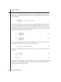
The usual, uncorrected binding energy would be calculated as:
∆E bind = E 1 – ( E 2 + E 3 )
where the energy subscripts refer to the calculations listed above. The counterpoise correction
to the binding energy expresses the artificial gain in energy of each molecular fragment when it
can use the basis functions of the other fragment in addition to its own basis functions:
∆E cp = ( E 4 – E 6 ) + ( E 5 – E 7 )
Calculated in this way, the counterpoise correction is a positive number, and it is added to
∆E bind to yield the final binding energy. Counterpoise corrections are often several kilocalories per mole in magnitude, and decrease as the size of the basis set increases.
In the input files for jobs 6 and 7, the atoms of one fragment must be marked as counterpoise
atoms (also called “ghost atoms”) so that only their basis functions are used. In Jaguar, a counterpoise atom is indicated by appending a @ to the atom label. For example, to calculate the
interaction energy of a water molecule with a methanol molecule, the zmat section for one
counterpoise job would have the atoms of for methanol marked as counterpoise atoms:
&zmat
O1@
H2@
C3@
H4@
H5@
H6@
O7
H8
H9
&
-0.3380316687
-0.3206434752
0.9752459717
0.9478196867
1.5357440779
1.5357440779
-0.4959747210
-1.0372322234
-1.0372322234
0.9068671477
-0.0520359937
1.3666159794
2.4513855069
1.0497731323
1.0497731323
-1.9447535985
-2.1494734847
-2.1494734847
0.0000000000
0.0000000000
0.0000000000
0.0000000000
-0.8817844743
0.8817844743
0.0000000000
0.7574958845
-0.7574958845
In the other counterpoise job, the zmat section would have the atoms of the water molecule
marked as counterpoise atoms:
&zmat
O1
H2
C3
H4
H5
H6
O7@
H8@
H9@
&
-0.3380316687
-0.3206434752
0.9752459717
0.9478196867
1.5357440779
1.5357440779
-0.4959747210
-1.0372322234
-1.0372322234
0.9068671477
-0.0520359937
1.3666159794
2.4513855069
1.0497731323
1.0497731323
-1.9447535985
-2.1494734847
-2.1494734847
0.0000000000
0.0000000000
0.0000000000
0.0000000000
-0.8817844743
0.8817844743
0.0000000000
0.7574958845
-0.7574958845
Jaguar 7.5 User Manual
15
Chapter 2: Running Jaguar From Maestro
You can also indicate counterpoise atoms in an atomic section by setting their nuclear charge
to zero in the ’charge’ column (see Section 8.8.3 on page 230).
To automate the calculation of a counterpoise-corrected binding energy for a complex
consisting of two non-covalently bound molecules, you can choose Counterpoise from the
Jaguar submenu of the applications menu. The panel that opens can be used to set up and run
the counterpoise job, which uses the Jaguar batch script counterpoise.py. This panel
contains only the Molecule, Theory, SCF, and Optimization tabs. See Section 10.2.4 on
page 289 for details on the counterpoise.py script, which you can also use from the
command line.
For LMP2 calculations (see Section 3.5 on page 42), the LMP2 correction is already designed
to avoid basis set superposition error, so we advise computing only the SCF counterpoise
correction term.
2.4.8
Specifying Coordinates for Hessian Refinement
If you are optimizing a molecular structure to obtain a transition state, you might want to refine
the Hessian used for the job. Section 4.3 on page 78 explains the methods used for transitionstate optimizations, including Hessian refinement. This subsection explains only how to edit
your input to specify particular coordinates for Hessian refinement. (Whether or not you refine
particular coordinates, you can specify a certain number of the lowest eigenvectors of the
Hessian for refinement, as described in Section 4.3.4 on page 82—the Hessian can be refined
in both ways in the same job.)
If you type an asterisk (*) after a coordinate value, Jaguar computes the gradient of the energy
both at the original geometry and at a geometry for which the asterisk-marked coordinate has
been changed slightly, and uses the results to refine the initial Hessian to be used for the optimization. To request refinement of a coordinate whose value is set using a variable, add an
asterisk to the end of the variable setting in the variable definition section.
For instance, either of the following two input geometries will have the same effect: a job that
includes Hessian refinement will use both O–H bonds and the H–O–H angle in the refinement.
O1
H2
H3
O1
O1
1.1*
1.1*
H2
108.0*
or
O1
H2
O1
ohbond
H3
O1
ohbond
ohbond = 1.1*
16
H2
Jaguar 7.5 User Manual
108.0*
Chapter 2: Running Jaguar From Maestro
Molecular symmetry or the use of variables, either of which may constrain several coordinate
values to be equal to each other, can reduce the number of coordinates actually used for refinement. For example, for the second water example shown above, only two coordinates are actually refined (the O–H bond distance, which is the same for both bonds, and the H–O–H angle).
The same would be true for the first example if molecular symmetry were used for the job.
2.5
Reading Files
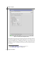
If you already have Jaguar input files containing geometries (either with or without information on the type of calculation to perform), you can read them using the Jaguar Read dialog
box, which you open by clicking the Read button in the Jaguar panel. This dialog box is a file
selector with the usual file browsing tools: a Filter text box, a Directories list, a Files list, and a
Selection text box. By default, information is displayed for the current working directory.
When you read a Jaguar input file, you can read the geometry only, or you can read the entire
input file. To read just the geometry, choose Geometry only from the Read as option menu. To
read the entire input file, choose Geometry and settings from the Read as option menu. If you
read in a geometry only from a file, Jaguar also tries to obtain information on the molecular
charge. If you read the geometry and settings, the settings are used to determine the Jaguar
task, which might not be the task with which you opened the Jaguar panel. For example, if you
chose Single Point Energy, then read an input file for a geometry optimization including the
settings, the task is reset to Optimization.
Figure 2.3. The Jaguar Read dialog box.
Jaguar 7.5 User Manual
17
Chapter 2: Running Jaguar From Maestro
The structures in the input file are added as entries in the Project Table, named with the stem of
the input file name by default. For example, reading h2o.in creates an entry named h2o.
To read geometries from files generated or used by other programs, you must import them into
Maestro using the Import panel. The files are imported using the file format conversion
program, Babel [26], and must be in a format recognized by Babel. Maestro does not read any
information other than the geometry from these files. If you want other information, such as a
Hessian, you can cut and paste it into a Jaguar input file.
2.6
Setting Charge and Multiplicity
Apart from the geometry, the main setting that you might want to make in an otherwise default
calculation is to set the molecular charge and the spin multiplicity. You can set these quantities
in the Molecule tab. The default molecular charge is determined by the formal charges on the
atoms in the Workspace. The default spin multiplicity is 1 (singlet) if the molecule has an even
number of electrons, and 2 (doublet) if it has an odd number of electrons. You can change the
charge by entering a value in the Molecular charge text box,2 and you can change the spin
multiplicity by entering a value in the Spin Multiplicity (2S+1) text box.3 The spin multiplicity is
always displayed in this text box. If the molecular charge and spin multiplicity settings you
make do not agree with your molecular input—for instance, if your molecule has an odd
number of electrons and you set the spin multiplicity to 1—Maestro warns you of the inconsistency, and you must choose consistent values to submit a job.
The charge and spin multiplicity can be stored in the Project Table as properties of the molecule. To do so, click Create Properties. For any entry that has these properties set, you can set
the charge and spin multiplicity for the calculation by selecting Use charge and multiplicity
from Project Table.
2.7
Cleaning up Molecular Geometries
The molecular geometry sometimes needs improvement before you perform calculations. For
example, it might not have the desired molecular symmetry, or it might be far from the
minimum (or transition state). Maestro has options to clean up the geometry for calculations in
both of these cases. The options are available from the Build panel, which you can open by
clicking the Open/Close Build panel toolbar button in the main window.
2.
3.
18
Keyword molchg in the gen section.
Keyword multip in the gen section.
Jaguar 7.5 User Manual
Chapter 2: Running Jaguar From Maestro
2.7.1
Quick Geometry Optimization
You can clean up the geometry by clicking the Clean up geometry button on the Build toolbar:
Maestro first performs a quick charge-equilibration (Qeq) calculation to obtain partial charges
for all atoms in the system, and then uses those charges in an energy minimization, based on
Goddard and Rappe’s Universal Force Field (UFF). Because UFF includes parameters for all
elements in the periodic table, it can be used for inorganic complexes as well as organic
compounds. During the UFF minimization, a status box is displayed. To stop the minimization,
click Stop in this status box.
The convergence criteria for the cleanup minimization are deliberately set fairly loose, so that
even fairly large systems can be optimized interactively. The practical size limit is about 300
atoms. In addition, a time limit is imposed on the minimization to keep it from running excessively long. As a result, you might find that the geometry continues to change if you perform a
second cleanup minimization on a cleaned-up structure.
UFF cleanup minimization is useful for quickly bringing a distorted molecule back into the
neighborhood of the ab initio minimum-energy geometry, in preparation for full ab initio
geometry optimization. However, it is no substitute for ab initio optimization because UFF is a
relatively simple force field. It is probably a good idea to perform a cleanup minimization after
creating a new molecule in the Build panel. On the other hand, performing a cleanup minimization on a molecule that has already undergone ab initio minimization is likely to move the
molecule away from the ab initio minimum. Also, you should be careful to avoid cleaning up a
structure that has been prepared as an initial guess for a transition-state search.
2.7.2
Symmetrization
By default, Jaguar takes advantage of molecular symmetry4 whenever possible, in order to save
CPU time. Both Abelian and non-Abelian point groups are recognized. Generally, you should
symmetrize the geometry if you plan to use symmetry in the calculation itself. Otherwise, the
input coordinates may not be accurate enough for the desired symmetry to be recognized.
You can symmetrize the molecule by choosing Symmetrize Workspace from the Edit menu.
The Symmetrize Workspace dialog box is displayed.
The point group symmetry is determined as follows. After the molecule is translated so that the
center of mass is at the origin of the coordinate system and rotated so that the principal axes of
4.
Keyword isymm = 8 in the gen section.
Jaguar 7.5 User Manual
19
Chapter 2: Running Jaguar From Maestro
inertia are aligned on the coordinate axes, symmetry operations (reflections, rotations, and
inversions) are applied to determine the point group of the molecule.
When Maestro checks whether a symmetry operation produces an equivalent structure, the
coordinates of the two structures only have to be the same to within a prescribed tolerance, that
is, each pair of symmetry-related atoms is within a distance specified by the tolerance. The
value of the tolerance can be specified in the Tolerance text box, and is 0.04 Å by default. This
value ensures that the highest symmetry is found in most cases. By changing the value and
clicking the Find Point Group button, you can determine whether there is a lower (or higher)
symmetry point group that approximately describes the structure, and use that group to
symmetrize the molecule instead of the default.
The tolerance is also used when the molecule is symmetrized. After translation and rotation,
the coordinates of the atoms are adjusted to reflect the symmetry group accurately. The
maximum displacement permitted is the tolerance specified. A large tolerance yields the
highest symmetry, but may cause the coordinates to be changed significantly. A small tolerance
may yield a lower symmetry, but results in smaller coordinate changes. The main Jaguar
programs use a small tolerance (1.0 x 10⁻⁶ bohr), which should result in molecular energy
changes of 1 microHartree or less.
You can turn the use of symmetry off5 in the Molecule tab. For methods such as GVB, LMP2,
GVB-LMP2, and for some properties, such as IR intensities or hyperpolarizabilities, symmetry
is not yet implemented and is disabled automatically for the job.
If you are comparing calculations from geometries that differ only slightly, you must use
caution when symmetrizing coordinates. For example, a small symmetry-breaking change can
be removed if its magnitude is smaller than the tolerance you have set, which establishes what
changes are acceptable. In this case, you should inspect the symmetrized coordinates in the
Edit Job dialog box to insure that symmetrizing had the desired effect and did not discard any
important information about the molecular geometry.
2.8
Writing Files
When you are satisfied with the molecular geometry and the settings that you have made, you
can either run the job, or save the geometry and settings for later use. Running jobs is described
in the next section. To save your input, click the Write button at the foot of the Jaguar panel.
The Jaguar Write dialog box is displayed. This dialog box is a file selector with the usual file
browsing tools: a Filter text box, a Directories list, a Files list, and a Selection text box. By
default, information is displayed in the lists and the filter for the current working directory.
5.
20
Keyword isymm = 0 in the gen section.
Jaguar 7.5 User Manual
Chapter 2: Running Jaguar From Maestro
Figure 2.4. The Jaguar Write dialog box.
If you want to write a Jaguar input file containing the geometry and the settings, choose Jaguar
input from the File Format option menu. When you click OK, a Jaguar input file is created that
is suitable for running a calculation, whether from Maestro or from the command line.
If you want to use the settings for a series of calculations on different molecules, you can write
a batch script, by choosing Jaguar batch script from the File Format option menu. When you
click OK, a Jaguar batch script is created that contains settings (gen section) and batch
commands, but no geometry, so that you can run this script with any geometry. To make use of
this script, you can select Run Batch File from the Jaguar submenu of the Applications menu in
the main window.
You can also use Maestro to export structures to a variety of formats, using the Babel file
conversion program (see Section 10.1.5 on page 279). See Chapter 3 of the Maestro User
Manual for more information on exporting structures.
2.9
Running Jobs
Maestro provides several ways of running Jaguar jobs. You can select a task from the Jaguar
submenu of the Applications menu, make settings, then start the job; you can select a set of
preexisting input files and run them as a single job by selecting Run Input Files from the Jaguar
submenu; or you can run a job using a preexisting Jaguar batch file with one or more structures
as input by selecting Run Batch File from the Jaguar submenu.
Jaguar 7.5 User Manual
21
Chapter 2: Running Jaguar From Maestro
Figure 2.5. The Start dialog box.
Whenever you run a calculation with multiple structures as input that does not have any geometry-dependent settings, a Jaguar batch script is created to run the calculation on each structure.
You can submit a job either from Maestro or from the command line. Information on submitting jobs from the command line with the jaguar run command can be found in Section 10.1
on page 273. This section describes the submission of jobs from Maestro.
Regardless of what kind of job you run or where the input is obtained from, you can submit the
Jaguar job by clicking the Start button in the relevant panel. The Start dialog box (Figure 2.5)
is displayed, in which you can enter information on how and where to launch a job. This dialog
box has two sections: the Output section and the Job section. For more detailed information on
this dialog box, see Section 4.2 of the Job Control Guide.
2.9.1
Output Handling
In the Output section you can choose how the results are incorporated into Maestro at the end
of the job, using the Incorporate option menu. The four options are described in Section 4.8 of
the Job Control Guide.
If your job input is a scratch entry, an alert box (Figure 2.6) is displayed when you click Start,
before the Start dialog box is displayed. This box prompts you to create a named entry from
the scratch entry. If you then click Run With Scratch, Do not incorporate is automatically
selected in the Start dialog box, and the Incorporate controls are unavailable. The job can be
run, but it cannot be incorporated into the project.
The local directory where input and output files created by Jaguar are written is determined by
the setting in the Directory tab of the Preferences panel. The default local job directory is the
directory from which you read the input file, if you read one, or the directory you were in when
you started Maestro. See page 29 of the Maestro Overview for more information.
22
Jaguar 7.5 User Manual
Chapter 2: Running Jaguar From Maestro
Figure 2.6. Scratch entry alert box.
2.9.2
Job Submission Options
In the Job section, you can provide a job name, select the execution host, the number of
processors, and the scratch directory. The choices available in the Job section depend on the
schrodinger.hosts configuration file. See Section 2.1 of the Job Control Guide for more
information on this file.
The job name can be entered in the Name text box. The names of the input, output, and log
files for your job depend on this name: the Jaguar input file is named jobname.in, the output
file is named jobname.out, and the log file is named jobname.log. For instance, if the job
name is h2o, the results are stored in a file called h2o.out within the local job directory. If the
structure is a scratch entry, a default name is selected.
The execution host (the machine that the job will run on) can be selected from the Host option
menu. This menu lists all the hosts available in the schrodinger.hosts file. The default
execution host is localhost, which means the machine on which Maestro is running. The host
name is followed by the number of available processors in parentheses.
If the host you choose has multiple processors, you can run Jaguar in parallel on that host. You
can enter the number of processors to use in the CPUs text box. The default is one processor.
Note:
You can distribute batch jobs over multiple processors only if you are using the default
batch script or the current settings for the batch script. The exception is pKa jobs,
which can be run on two processors, because they consist of two independent jobs.
You cannot run MPI parallel jobs as batch jobs.
The Scratch directory option menu displays a list of directories on the execution host that can
be used to store temporary files. A subdirectory with the given job name (h2o, for example) is
created within the temporary directory, and the files from the calculation are stored in this
subdirectory. If the subdirectory and directory do not have sufficient disk space for the job, the
job fails. If the temporary directory does not exist, you should create it, or choose a directory
which already exists. If none of the temporary directory choices already exist and you do not
want to create the necessary directories, you can change the schrodinger.hosts file so that
the option menu offers you different choices (see Section 2.1 of the Job Control Guide).
Jaguar 7.5 User Manual
23
Chapter 2: Running Jaguar From Maestro
2.9.3
Starting and Monitoring Jobs
When you are satisfied with the settings, start the job by clicking Start. The Monitor panel
opens, and displays the Jaguar log file for the job. As the job runs, this file is updated. If you
close the Monitor panel, the updating ceases. You can reopen the panel later by choosing
Monitor Jobs from the Applications menu. To monitor the job again, select it in the table and
click Monitor. See the Chapter 5 of the Job Control Guide for more information on job control
and monitoring.
Any additional jobs that you submit run concurrently. If you exit Maestro, any Jaguar jobs still
running continue to run to completion.
2.10 Running Jaguar Batch Jobs
You can run multiple Jaguar calculations in a single run using Jaguar batch scripts. Some of the
kinds of calculations you can run with a batch script are:
• Multiple independent jobs with predetermined input files
• The same type of job for several input geometries
• A series of jobs in which later jobs use files generated during earlier jobs
Several Jaguar batch scripts are included with Jaguar. You can also write your own batch
scripts or save job settings as a batch script in the Jaguar Write dialog box. Maestro writes
temporary batch scripts and runs a batch job whenever you run jobs with multiple structures as
input that do not have geometry-dependent settings. Section 10.2 on page 282 provides details
on batch scripts.
Jaguar batch jobs can be run from the Run Batch File panel, which you open by choosing Run
Batch File from the Jaguar submenu of the Applications menu. To run a batch job, you must
select a script and a source of structures, and start the job. If you select Jaguar input files for the
structural input, you can choose whether to use or ignore the settings in the input files.
Figure 2.7. The Run Batch File panel.
24
Jaguar 7.5 User Manual
Chapter 2: Running Jaguar From Maestro
Figure 2.8. The Select Batch Script panel.
To select a script, you can enter the path in the Script text box, or click Browse and choose a
script in the Select Batch Script panel. This panel is a file selector with the usual file browsing
tools. By default, information is displayed in the lists and the filter for the current working
directory. To select one of the supplied Jaguar scripts, click Jaguar Scripts in the Directory
section, then select the script. When you select a script, the Notes text area shows comments
from the batch script.
When you have chosen the directory, choose a script from the list of scripts, then click OK. The
built-in scripts are described briefly in Table 2.1.
The input files that you select can be pre-existing input files, or files created from the current
structure in the Workspace or from Project Table entries. These choices are available from the
Source of structures option menu in the Run Batch File panel. If you choose Workspace or
Selected entries, the structures are written to a single Maestro file, and the Jaguar input files
are created later by the batch facility.
To select pre-existing files, choose Selected structure files from the Source of structures option
menu, then enter a comma-separated list of file names in the Files text box, or click Browse.
The Browse button opens a standard file selector, labeled Select Batch Inputs, with the current
directory and its files listed. You can select either Jaguar input files or Maestro files for input. If
you select Maestro files, Jaguar input files are constructed later. To select multiple files, use
Jaguar 7.5 User Manual
25
Chapter 2: Running Jaguar From Maestro
SHIFT to select a range of items and CTRL to select or deselect a single item without affecting
other items. When you have made a selection, click OK. The input files are passed to the batch
script in the order in which they appear in the list. To process input files in a particular order,
you must name them so that they appear in the correct order in the list.
After you finish selecting the batch script and input files, click Start to launch the batch job.
The Monitor panel opens and shows the batch log file (.blog) for the batch job, which logs the
completion of each Jaguar job launched from the batch script. The information is automatically
updated as the Jaguar jobs run.
Table 2.1. Description of built-in batch scripts
Script
Description
JOBS.bat
Run a sequence of jobs specified by the input files.
geopt-DFT-I.bat
Preoptimize a geometry at the BLYP/6-31G level, then optimize at the
BLYP/6-31G* level.
geopt-DFT-II.bat
Do geometry preoptimizations at the HF/6-31G and BLYP/6-31G*
level, then optimize at the B3LYP/cc-pVTZ(-f) level.
geopt-DFT-III.bat
Do geometry preoptimizations at the HF/6-31G, BLYP/6-31G* and
B3LYP/6-31G* level, then optimize at the B3LYP/cc-pVTZ(-f) level.
j2.bat
Run a J2 theory calculation [27].
pka.bat
Run a pKa calculation. See Chapter 13 for details.
counterpoise.py
Run a counterpoise calculation. See Section 2.4.7 and Section 10.2.4.
distributed_scan.py
Distribute a 1D or 2D scan job over multiple processors. Automatically used from Maestro when multiple processors are requested. See
Section 10.2.4.
hydrogen_bond.py
Calculate binding energy of two molecules that are hydrogen-bonded.
See Section 2.13 and Section 10.2.4.
2.11 Output
A Jaguar log file contains comments on the progress of a job. If the job was started from
Maestro, the log file is written to the local job directory. The log file notes when each section
of Jaguar is complete, as well as noting data from each iteration in an SCF calculation as it is
calculated. You can view this file in the Monitor panel, which is displayed when a job is
launched or when you choose Monitor from the Applications menu in the main window. See
Section 5.7 on page 136 for more information on this file.
26
Jaguar 7.5 User Manual
Chapter 2: Running Jaguar From Maestro
The primary Jaguar output is contained in the output file, which is created in the scratch directory of the host on which the calculation is run, and is copied back to the local host when the
job finishes. The output file is described in Chapter 5.
2.12 J2 Theory Calculations
If you want to calculate energies accurately, you can perform J2 theory calculations [27] using
a predefined batch script. The J2 batch script performs a B3LYP/6-31G* geometry optimization and frequency calculation, followed by single point GVB/LMP2 calculations using the ccpvtz(-f) and cc-pvtz++ basis sets at the B3LYP optimized geometries. These single-point
calculations are used to determine a basis set correction energy. A parameterized electron-pair
correction energy is also added. The final J2 energy is an absolute enthalpy at 298K. The finite
temperature effects are calculated from the B3LYP frequencies. The J2 results do not include a
standard heat of formation, because the relevant calculations for the constituent atoms are not
made. J2 theory calculations cannot be performed for structures containing atoms that are
heavier than Ar.
To run J2 theory calculations, choose J2 from the Jaguar submenu of the Applications menu.
The Jaguar panel has only the Molecule and SCF tabs, because all other input is predefined.
When you have selected the structures and made any settings, click Start.
You can also use the jaguar j2 command to run the calculation from the command line:
jaguar j2 [options] input-files
This command executes jaguar batch. You can run the calculation on a remote host or in
parallel by specifying the relevant command options. See Section 10.2 on page 282 for details
on jaguar batch commands, including command line options.
2.13 Binding Energies of Hydrogen-Bonded Complexes
To calculate an accurate binding energy for an intermolecular hydrogen-bonded complex, you
can use the Jaguar batch script hydrogen_bond.py (see Section 10.2.4.2 on page 290 for
instructions), either from Maestro or from the command line (on UNIX). This script automates
a multi-step protocol in which the binding energy is calculated using two correlation-consistent
basis sets (cc-pVTZ(-f) and cc-pVQZ(-g)) and LMP2 theory, including corrections for basis
set superposition error. The final correction to the binding energy uses two parameters from a
fit of the energies to reference energies that were obtained from CCSD(T) calculations extrapolated to the basis set limit. The binding energies are accurate to within 0.5 kcal/mol when
compared to the extrapolated CCSD(T) energies.
Jaguar 7.5 User Manual
27
Chapter 2: Running Jaguar From Maestro
Figure 2.9. The Jaguar panel for hydrogen bond calculations.
The protocol is based on that described in Ref. 28, except that all geometry optimizations are
carried out using X3LYP/6-31G** instead of LMP2/cc-pVTZ(-f). The X3LYP density functional gives very good geometries for hydrogen-bonded complexes and is much faster than
LMP2. The energy calculations, however, are still carried out using LMP2 with the
cc-pVTZ(-f) and cc-pVQZ(-g) basis sets.
An option is provided to use the DFT energies rather than the LMP2 energies. In a test for a
series of ten hydrogen-bonded complexes, the RMS error using the DFT energies was 0.72
kcal/mol, while the RMS error using the default LMP2 method was 0.34 kcal/mol. Other
options are provided to control the optimization process.
28
Jaguar 7.5 User Manual
Chapter 2: Running Jaguar From Maestro
To run a hydrogen bond binding energy calculation, choose Hydrogen Bond from the Jaguar
submenu of the Applications menu.
The panel that opens has controls for defining the molecular state, and for choosing which
structures to optimize:
• Optimize all structures—Optimize the complex and the two molecules that make up the
complex.
• Optimize individual molecules, but not the complex—Optimize the two molecules that
make up the complex, but not the complex itself, which retains its input geometry.
• Do not optimize any structures—Use the input geometry for all calculations: do not perform any optimizations.
• Freeze all torsions during optimizations—Optimize the complex and the two molecules
that make up the complex, but freeze all torsions (dihedral angles) in the optimization and
optimize only the bond lengths and bond angles. This helps convergence with weaklybound systems.
You can also select Fast mode to use the DFT energies instead of the LMP2 energies.
When the job finishes, the optimized structure of the complex is incorporated into the project,
with the binding energy, in kcal/mol, as a property.
Jaguar 7.5 User Manual
29
30
Jaguar 7.5 User Manual
Jaguar User Manual
Chapter 3
Chapter 3:
Options
Jaguar provides a wide range of options for performing different kinds of calculations, for
controlling the convergence of calculations, and for controlling the output of calculations.
Most of these options can be set in the various tabs of the Jaguar panel. The options that are
common to nearly all calculations are set in the following six tabs:
•
•
•
•
Molecule—charge, spin, symmetry, basis set.
Theory—HF, DFT, LMP2, GVB, GVB-LMP2, CIS, restricted/unrestricted SCF.
SCF—SCF convergence
Properties—frequencies, surfaces, ESP charges, Mulliken populations, NBO analysis,
multipole moments, polarizabilities
• Solvation—solvent, reference energy
• Output—printout options, output files
The remaining tabs that can appear in the Jaguar panel vary according to the task: Optimization, Transition State, IRC, Scan. These tabs are described in Chapter 4, along with other information about optimizations and scans. Output options are described in Chapter 5. This chapter
describes the settings that can be made in the Molecule, Theory, SCF, Properties, and Solvation
tabs.
The footnotes in this chapter indicate the Jaguar input file keywords and sections that correspond to settings made in the GUI. If you are working from the GUI, you can ignore these
footnotes, but you may find them helpful if you decide to use input files to submit jobs without
using the GUI, or if you want to edit keywords directly by using the Edit Job window described
in Section 2.3 on page 8.
3.1
Molecule Settings
The top part of the Molecule tab provides controls for the molecular charge, the spin multiplicity, and the application of molecular symmetry. Setting charge and spin multiplicity was
discussed in Section 2.6 on page 18. Briefly, you can enter the charge and spin multiplicity in
text boxes, or you can use values that are listed in the Project Table. If you choose the latter,
you can create the corresponding properties and enter values for them if they don’t exist.
By default, Jaguar takes advantage of molecular symmetry in order to obtain CPU savings.
Both Abelian and non-Abelian point groups are recognized. You can select whether to use the
full symmetry,1 Abelian symmetry (D2h and subgroups),2 or turn the use of symmetry off3 in
Jaguar 7.5 User Manual
31
Chapter 3: Options
the Symmetry option menu. For information on how to make sure the symmetry of your input
structure is treated as you expect, see Section 2.7.2 on page 19.
For some calculations, including GVB, LMP2, GVB-LMP2 calculations and calculations of IR
intensities or hyperpolarizabilities, symmetry is not implemented and is disabled automatically
during the job.
3.2
Basis Sets
In the lower part of the Molecule tab, you can choose a basis set4 from the three option menus
labeled Basis Set, Polarization, and Diffuse. The Basis Set option menu provides access to all
the basis sets available to Jaguar. If an option or menu is dimmed, it is incompatible with the
rest of your input (for instance, the basis set could be missing basis functions for some atom or
atoms in your molecule). Basis sets that do not have pseudospectral grids and dealiasing functions are listed in italics in the Basis Set option menu.
If you do not choose a basis set for a calculation, Jaguar uses the 6-31G** basis set if 6-31G**
basis functions are available for all atoms in the input, and otherwise uses the LACVP** basis
set by default. These basis sets are described in more detail below.
The Polarization option menu provides the choices none, *, and **. In general, the ** option
places polarization functions on all atoms except for transition metals, and the * option places
polarization functions on all atoms except for transition metals, H, and He. The tables below
describe in detail the atoms that have polarization functions in each basis set. The correlationconsistent basis sets (cc-pVnZ) are intrinsically polarized.
The Diffuse option menu provides the choices + and ++. The ++ option places diffuse functions
on all atoms, while the + option places diffuse functions on all atoms except H and He. Diffuse
functions are useful for calculations on van der Waals complexes or molecules that include
atoms with negative charges.
For the basis set that you select, a message giving the number of functions and stating whether
pseudospectral grids are available and whether ECPs are used is displayed below the controls.
Table 3.1 lists the available basis sets in Jaguar that do not use effective core potentials. The
table indicates the atoms these basis sets can describe and shows which sets include the options
of polarization and diffuse functions. The cc-pVDZ and cc-pVTZ basis sets include polarization functions by definition.
1.
2.
3.
4.
32
Keyword isymm = 8 in the gen section.
Keyword isymm = 8 and idoabe=1 in the gen section.
Keyword isymm = 0 in the gen section.
Keyword basis in the gen section.
Jaguar 7.5 User Manual
Chapter 3: Options
Figure 3.1. The Molecule tab.
Table 3.1 also indicates the method used for the calculation: the fast pseudospectral method or
the slower analytic method, in which four-center, two-electron integrals are computed explicitly. The analytic method is used only when optimized pseudospectral grids and dealiasing
function sets for one or more atoms in the molecule are not available. For molecules whose
atoms are all in the range H–Ar in the periodic table, we recommend using the 6-31G** basis
set (the default choice), which is one basis set that permits pseudospectral calculations.
The column headed “# of d fns.” indicates whether d shells include the five real spherical functions d xy , d xz , d yz , d x2 – y2 , and d 2 z 2 – x2 – y2 , all with the same angular momentum (l = 2), or
whether d shells include the six Cartesian d functions d x2 , d y2 , d z 2 , d xy , d xz , and d yz . This
Jaguar 7.5 User Manual
33
Chapter 3: Options
choice also affects the dimension of the Fock matrix for diagonalization. To override this selection, select the Number of D functions option that corresponds to your preference, or set the
keyword numd in the gen section of the input file, as described in Section 8.5.16 on page 200.
The orbital coefficients are always printed out in terms of the six Cartesian functions. For basis
sets with f functions, the real spherical set of 7 f functions is always used.
The references describing the basis sets are in the References list at the back of this manual.
Table 3.1. Available basis sets that do not include effective core potentials
34
Basis Set
Atoms
Included
Options
Method
# of
d fns.
Refs.
STO-3G
H-Xe
* (Na-Xe)
analytic
5
79-83
3-21G
H-Xe
* (Na-Ar),
+ (Li-Ar),
++ (H-Ar)
H–Ar pseudospectral (analytic
with + or ++), K–Xe analytic
6
84-86
4-21G
H-Ne
*, **
analytic
6
87
6-21G
H-Ar
*, **
analytic
6
84-86
4-31G
H-Ne
*, **
analytic
6
88-93
6-31G
H-Ar
*, **; +, ++
pseudospectral
6
89-94
6-311G
H-Ar
*, **, +, ++
pseudospectral
5
96-99
6-311G-3df3pda
H-Ar
+, ++
analytic
5
96-99
6-31G(tm)
H-Zn
*, **; +, ++
for H-Ar
H-Ar pseudospectral, K-Zn analytic
6
89-95
m6-31G(tm)
K-Zn
analytic
6
100
D95V
H, Li-Ne
*, **
analytic
6
101
D95
H, Li-Ne,
Al-Cl
*, **
H, Li, C-F, Si-Cl pseudospectral,
others analytic
6
101
MSV
H-Ru, Pd-Xe
analytic
5
102
cc-pVDZ
H-He, B-Ne,
Al-Ar
+, ++
H, C-F, Si-Cl pseudospectral,
others analytic; +, ++ analytic
5
103106
cc-pVDZ(-d)
(without d
functions)
H-He, B-Ne,
Al-Ar
+, ++
H, C-F, Si-Cl pseudospectral,
others analytic; +, ++ analytic
5
103106
cc-pVTZ
H-Ar, Ca,
Ga-Kr
+, ++
H, He, B-Na, Al-Ar, As-Br
pseudospectral, others analytic
5
103106
Jaguar 7.5 User Manual
Chapter 3: Options
Table 3.1. Available basis sets that do not include effective core potentials (Continued)
Basis Set
Atoms
Included
Options
Method
# of
d fns.
Refs.
cc-pVTZ(-f)
(without f
functions)
H-Ar, Ca,
Ga-Kr
+, ++
H, He, B-Na, Al-Ar, As-Br
pseudospectral, others analytic
5
103106
cc-pVQZ(-g)
(without g
functions)
H-Ar, Ca,
Ga-Kr
+, ++
H, C-F, S, Cl, Br, pseudospectral,
others analytic; +, ++ analytic
5
103
MIDIX
H, Li, C-F,
Si-Cl, Br, I
H, C-F, P-Cl pseudospectral; Li,
Si, Br, I analytic
5
107109
TZV
H-Kr
*,** (Sc-Zn
p only)
analytic
5
110
TZV(f)
H-Kr
*,* (Sc-Zn p
and f)
analytic
5
110
a. This basis is referred to in the literature as 6-311G(3df-3pd).
The other available basis sets, which are listed in Table 3.2, include effective core potentials
(ECPs). The names of eight of these basis sets begin with “LA” to indicate they were developed at Los Alamos National Laboratory. If the next character in the name is a “V,” the basis
set is valence-only, containing only the highest s and p shells for main group atoms and the
highest s, p, and d shells for transition metals. For example, 5s and 5p would be included for
tellurium, and 6s, 5d, and 6p for tungsten. “LAV1” indicates that the basis set has been fully
contracted to form a minimal basis set, “LAV2” that the last Gaussian has been uncontracted to
form a double zeta basis, and “LAV3” that all of the s functions and the last p and d Gaussian
have been uncontracted.
Names starting with “LACV” indicate that the basis set also includes the outermost core
orbitals (e.g., 5s5p6s5d6p for W). The last letter in each LA basis set name refers to the basis
set used for atoms not described by ECPs: S indicates the STO-3G basis set, D indicates the
D95V basis set, and P indicates the 6-31G set developed by Pople and coworkers. (Note that in
addition, for some atoms, the LACVD and LACVP basis sets use the same basis functions as
the LAV3D and LAV3P basis sets, respectively.)
The Los Alamos effective core potentials, which were developed by Hay and Wadt, include
one-electron mass-velocity and Darwin relativistic corrections for elements beyond Kr.
The Cundari-Stevens ECP basis set [118], named CSDZ, has been provided to cover the
lanthanides. This basis set uses a relativistic effective core potential for the inner core electrons
and treats the outer core and valence electrons with a 4s/4p/2d/2f basis set.
Jaguar 7.5 User Manual
35
Chapter 3: Options
Table 3.2. Basis sets contained in Jaguar that include effective core potentials
Basis Set
Atoms in ECP
Other Atoms
Options
Refs.
LAV1S
Na-La, Hf-Bi
H-Ne (STO-3G)
* (H-Ne)
111-112
LAV2D
Na-La, Hf-Bi
H, Li-Ne (D95V)
*, ** (H, Li-Ne)
111-112
LAV2P
Na-La, Hf-Bi
H-Ne (6-31G)
*, ** (H-Ne); +, ++
(H-Ne)
111-112
LAV3D
Na-La, Hf-Bi
H, Li-Ne (D95V)
*, ** (H, Li-Ne)
111-112
LAV3P
Na-La, Hf-Bi
H-Ne (6-31G)
*, ** (H-Ne); +, ++
(H-Ne)
111-112
LACVD
K-Cu, Rb-Ag,
Cs-La, Hf-Au
H, Li-Ne (D95V); Na-Ar,
Zn-Kr, Cd-Xe, Hg-Bi
(LAV3D)
*, ** (H, Li-Ne)
113
LACVP
K-Cu, Rb-Ag,
Cs-La, Hf-Au
H-Ar (6-31G); Zn-Kr,
Cd-Xe, Hg-Bi (LAV3P)
*, ** (H-Ar); +, ++
(H-Ar)
113
LACV3P
K-Cu, Rb-Ag,
Cs-La, Hf-Au
H-Ar (6-311G); Zn-Kr,
Cd-Xe, Hg-Bi (LAV3P)
*, ** (H-Ar); +, ++
(H-Ar, plus metal diffuse d)
114
cc-pVTZ-pp
Ga-Kr, In-Xe
H-Ar, Ca (cc-pVTZ)
+, ++
115-117
cc-pVTZ-pp(-f)
Ga-Kr, In-Xe
H-Ar, Ca (cc-pVTZ(-f))
+, ++
115-117
CSDZ
Ce-Lu
H-Ar (6-31G); Zn-Kr,
Cd-Xe, Hg-Bi (LAV3P);
K-Cu, Rb-Ag, Cs-La,
Hf-Au (LACVP)
*, ** (H-Ar); +, ++
(H-Ar)
118
ERMLER2
K-Lr
H-Ar: 6-31G
*, ** (H-Ar, Sc-Kr,
Y-Xe, Hf-Rn) +, ++
(H-Ar, Ga-Kr, In-Xe,
Tl-Rn)
119-126
The ECP basis set developed by Ermler and coworkers [119-124], named ERMLER2, is also
available. The basis set provided is the “small core” set that includes the outer core orbitals in
the valence space, in the same way as the LACV basis sets. The basis set is a double-zeta
contraction in which the outermost primitive function in each symmetry has been uncontracted. The core is treated by a relativistic effective core potential for all elements. For Tl-Rn
the refitted ECPs have been taken from Wildman et al. [125], but the basis set from the original
ECPs has been retained, because the new basis sets are much larger, and do not match the basis
sets for the other elements. Polarization and diffuse functions for the 4p, 5p, and 6p elements
and polarization functions for the 3d, 4d, and 5d elements have been added from the relativistic
all-electron double-zeta set of Dyall [126].
36
Jaguar 7.5 User Manual
Chapter 3: Options
In Table 3.2, the atoms described by the effective core potential are listed first, followed by the
atoms described by the alternate basis set or sets. The other table entries provide the same
information as that given in the previous table, except that the polarization functions are only
applied to atoms obtained from the non-ECP basis sets, with the exception of the ERMLER2
basis sets. All ECP basis sets use five d functions, as described earlier in this section.
Currently, the LACVP, LAV3P, LACV3P, and CSDZ basis sets use the pseudospectral method,
while all other ECP basis sets use the analytic method, with the exception of Br and I in the ccpVTZ-pp and cc-pVTZ-pp(-f) basis sets. We strongly recommend using either the LACVP or
the LACV3P basis set for non-lanthanide molecules containing atoms beyond Ar in the periodic table, especially for studies involving charge transfer, d0 metals, or correlated wave functions. The LACV3P basis set seems to give substantial improvements over the LACVP basis
set for HF, LDA, and B3LYP atomic state splittings. The LACV3P++ basis set, which includes
a diffuse d function on any metal atoms, is useful for calculations on anions or low-spin M(0)
complexes of the late first row metals.
3.3
Density Functional Theory (DFT) Settings
The density functional theory module in Jaguar allows you to employ a variety of functionals
to describe exchange and correlation for either open or closed shell systems. The theory is
described in Section 7.5 on page 160. This section describes how to set up a DFT calculation in
Jaguar. You can perform DFT geometry optimizations, solvation calculations, charge fitting,
and all other calculations and properties available for Hartree-Fock wave functions.
DFT calculations are selected by choosing DFT (Density Functional Theory) from the Level of
theory option menu in the Theory tab. When you make this choice, controls for DFT calculation are displayed below this menu.
If you are doing calculations for an open-shell molecule, you can run a spin-restricted5
(RODFT) or a spin-unrestricted6 (UDFT) calculation. The default is a spin-restricted calculation. To run a UDFT calculation, select Spin-unrestricted.
You can run calculations for excited states of a closed-shell molecule using time-dependent
density functional theory (TDDFT). TDDFT has been implemented in Jaguar [185] using the
Tamm-Dancoff approximation [30]. To run a TDDFT calculation, select Excited state
(TDDFT), then enter the number of excited states in the Number of excited states text box. You
should select more excited states than you are actually interested in, for two reasons. The first
is that the initial guess might not accurately reflect the final states, and the second is to ensure
that near-degeneracies are accounted for. You can also set the number of TDDFT iterations.
5.
6.
Keyword iuhf = 0 in the gen section.
Keyword iuhf = 1 in the gen section.
Jaguar 7.5 User Manual
37
Chapter 3: Options
Figure 3.2. The Theory tab showing DFT controls.
The Grid density menu determines the grid for DFT calculations. By default, DFT calculations
use grids with a medium point density, but finer density grids are also available. You can
choose between Medium,7 Fine,8 or Maximum9 grid density. If you read an input file that
contained some other grid density, the grid density is set to Other, otherwise this option is
unavailable. If you choose a grid density from this menu, the previous grid density specification is replaced.
7.
8.
9.
38
Keywords gdftmed = –10, gdftfine = –11, and gdftgrad = –12 in the gen section.
Keywords gdftmed, gdftfine, and gdftgrad = –13 in the gen section.
Keywords gdftmed = gdftfine = gdftgrad = –14 in the gen section.
Jaguar 7.5 User Manual
Chapter 3: Options
The most commonly used functionals can be selected from the option menus in the Functionals
section. There are three classes of functionals available: local density functionals, gradientcorrected pure density functionals, and hybrid functionals, which include a Hartree-Fock
exchange contribution as well as local and nonlocal functionals. Most of the hybrid methods
employ either the parameters developed for Becke’s three-parameter method [32, 33] (Becke
3) or the parameters developed for Becke’s Half & Half method [31]. The option menus also
contain some recently developed hybrid and non-hybrid functionals. The functionals available
from the option menus are described below.
LDA (Local Density Functionals)
Functionals with local exchange only:
• HFS10: Slater local exchange functional [34]
• Xalpha11: Xα local exchange functional [34]
Functionals with local exchange and local correlation:
• SVWN12: Slater local exchange functional [34], Vosko-Wilk-Nusair (VWN) local correlation functional [35]
• SVWN513: Slater local exchange functional [34], Vosko-Wilk-Nusair 5 (VWN5) local
correlation functional [35]
Gradient-Corrected Functionals
• BLYP14: Exchange: Slater local functional [34], Becke 1988 nonlocal gradient correction
[37]; correlation: Lee-Yang-Parr local and nonlocal functionals [38]
• BPW9115: Exchange: Slater local functional [34], Becke 1988 nonlocal gradient correction [37]; correlation: Perdew-Wang 1991 GGA-II local and nonlocal functionals [36]
• BP8616: Exchange: Slater local functional [34], Becke 1988 non-local gradient correction
[37]; correlation: Perdew-Zunger 1981 local functional [39], Perdew 1986 gradient correction functional [40]
• BP86-VWN517: Exchange: Slater local functional [34], Becke 1988 nonlocal gradient correction [37]; correlation: Vosko-Wilk-Nusair (VWN) local functional [35], Perdew 1986
gradient correction functional [40]
10.
11.
12.
13.
14.
15.
16.
17.
Keyword dftname = hfs in the gen section.
Keyword dftname = xalpha in the gen section.
Keyword dftname = svwn in the gen section.
Keyword dftname = svwn5 in the gen section.
Keyword dftname = blyp in the gen section.
Keyword dftname = bpw91 in the gen section.
Keyword dftname = bp86 in the gen section.
Keyword dftname = bp86-vwn5 in the gen section.
Jaguar 7.5 User Manual
39
Chapter 3: Options
• PWPW9118: Exchange: Slater local functional [34], Perdew-Wang 1991 gradient correction functional [36]; correlation: Perdew-Wang 1991 GGA-II local and nonlocal functionals [36]
• PBE19: Perdew-Burke-Ernzerhof local and nonlocal exchange and correlation functional
[47]
• HCTH40720: Hamprecht-Cohen-Tozer-Handy functional [45] including local and nonlocal exchange and correlation, reparametrized with a training set of 407 molecules by
Boese and Handy [46]
• M06-L21: Parameterization by Zhao and Truhlar of various functionals that include gradient and kinetic energy spin density functionals [56]
• OLYP22: Exchange: Slater local functional [34], OPTX nonlocal exchange of Handy and
Cohen [48]; correlation: Lee-Yang-Parr local and nonlocal functionals [38]
Hybrid Functionals
• B3LYP23: Exchange: exact HF, Slater local functional [34], Becke 1988 nonlocal gradient
correction [37]; correlation: Vosko-Wilk-Nusair (VWN) local functional [35], Lee-YangParr local and nonlocal functional [38]. See refs. 32 and 33.
• B3PW9124: Exchange: exact HF, Slater local functional [34], Becke 1988 nonlocal gradient correction [37]; correlation: Perdew-Wang 1991 local and GGA-II nonlocal functional [36]
• B3P8625: Exchange: exact HF, Slater local exchange functional [34], Becke 1988 nonlocal gradient correction [37]; correlation: Vosko-Wilk-Nusair (VWN) local functional
[35], Perdew 1986 nonlocal gradient correction [40]
• B97-126: Reparametrization of Becke’s 1997 hybrid functional [42] by Hamprecht,
Cohen, Tozer, and Handy [45]
• B9827: Becke’s 1998 hybrid functional including the Laplacian of the density and kinetic
energy density terms as well as gradient terms [43]
• SB9828: Schmider and Becke reparametrization of Becke’s 1998 functional [44]
18.
19.
20.
21.
22.
23.
24.
25.
26.
27.
40
Keyword dftname = pwpw91 in the gen section.
Keyword dftname = pbe in the gen section.
Keyword dftname = hcth407 in the gen section.
Keyword dftname = m06-l in the gen section.
Keyword dftname = olyp in the gen section.
Keyword dftname = b3lyp in the gen section.
Keyword dftname = b3pw91 in the gen section.
Keyword dftname = b3p86 in the gen section.
Keyword dftname = b97-1 in the gen section.
Keyword dftname = b98 in the gen section.
Jaguar 7.5 User Manual
Chapter 3: Options
• BHandH29: 50% exact HF exchange, 50% Slater local exchange functional [34]
• BHandHLYP30: Exchange: 50% exact HF exchange, 50% Slater local exchange functional
[34]; correlation: Lee-Yang-Parr local and nonlocal functionals [38]
• X3LYP31: Extension of B3LYP by Xu and Goddard to include Perdew-Wang 1991 gradient correction exchange functional [36], with exchange parametrized to fit Gaussian
exchange density [52]
• MPW1K32: Reoptimization of mPW1PW91 functional parameter for prediction of reaction barrier heights, by Lynch, Fast, Harris, and Truhlar [51]
• MPW1PW9133: Hybrid functional including modification of Perdew-Wang gradient correction exchange functional, by Adamo and Barone [49]. Exchange: Exact HF exchange,
Slater local functional [34], Perdew-Wang 1991 gradient correction functional [36]; correlation: Perdew-Wang 1991 GGA-II local and nonlocal functionals [36]
• PWB6K34: Reoptimization of MPWB1K functionals for simultaneous accuracy of bond
energies, barrier heights, and nonbonded interactions, by Zhao and Truhlar [53]
• PW6B9535: Reoptimization of MPW1B95 functionals for simultaneous accuracy of bond
energies, barrier heights, and nonbonded interactions, by Zhao and Truhlar [53]
• PBE036: Functional due to Adamo and Barone [50] based on PBE functional. 25% exact
HF exchange, 75% PBE non-local exchange. Correlation: Perdew-Burke-Ernzerhof [47]
local and nonlocal correlation. Also known as PBE1PBE.
• M0537: Hybrid functional parametrized for broad accuracy, including noncovalent interactions, kinetics, and interactions with metals, by Zhao, Schultz, and Truhlar [54, 55]
• M05-2X38: Hybrid functional with larger HF exchange component, similar to M05 but
parametrized for nonmetals, by Zhao, Schultz, and Truhlar [54, 55]
• M06-HF39: Zhao and Truhlar functional with full HF exchange and M06 local functionals
that eliminates long-range self-interaction. [57]
28.
29.
30.
31.
32.
33.
34.
35.
36.
37.
38.
39.
Keyword dftname = sb98 in the gen section.
Keyword dftname = bhandh in the gen section.
Keyword dftname = bhandhlyp in the gen section.
Keyword dftname = x3lyp in the gen section.
Keyword dftname = mpw1k in the gen section.
Keyword dftname = mpw1pw91 in the gen section.
Keyword dftname = pwb6k in the gen section.
Keyword dftname = pw6b95 in the gen section.
Keyword dftname = pbe0 in the gen section.
Keyword dftname = m05 in the gen section.
Keyword dftname = m05-2x in the gen section.
Keyword dftname = m06-hf in the gen section.
Jaguar 7.5 User Manual
41
Chapter 3: Options
• M0640: Zhao and Truhlar functional, parametrized with metallic systems, for organometallic and inorganometallic chemistry and noncovalent interactions [58]
• M06-2X41: Zhao and Truhlar functional, parametrized for nonmetals, for main-group thermochemistry, kinetics, noncovalent interactions, and electronic excitation energies to
valence and Rydberg states [58]
• O3LYP42: Exchange: exact HF, Slater local functional [34], OPTX nonlocal functional of
Handy and Cohen [48]; correlation: Lee-Yang-Parr local and nonlocal functionals [38]
The names of the functionals in this list are valid values of the keyword dftname, which you
can use in the gen section of the input file to specify the functional. The names are case-insensitive.
3.4
Hartree-Fock and CIS Settings
In addition to selecting unrestricted (UHF) or spin-restricted (ROHF) treatment of open-shell
molecules, the controls available when you choose HF (Hartree-Fock) from the Level of theory
option menu allow you to set up configuration interaction singles (CIS) calculations for excited
states. These calculations are only available for a closed-shell Hartree-Fock reference wave
function. To do a CIS calculation, select Excited state (CIS).43 You can then enter the number
of states you want to generate in the Number of excited states text box,44 and set a limit on the
number of iterations in the diagonalization procedure in the Maximum CIS iterations text box.45
You should consider including more excited states than you need, to ensure that you include
the states of interest and cover any near-degeneracies.
3.5
Local MP2 Settings
The LMP2 (Local MP2) option46 of the Level of theory option menu allows you to set up a local
Møller-Plesset second-order perturbation theory [59–62] calculation. The local MP2 (LMP2)
method greatly reduces the basis set superposition errors that can arise from the canonical MP2
method [62]. The LMP2 method is much faster than canonical MP2, and typically recovers
98% of the canonical MP2 energy correction. The pseudospectral implementation of LMP2 is
described in Section 7.4 on page 157.
40.
41.
42.
43.
44.
45.
46.
42
Keyword dftname = m06 in the gen section.
Keyword dftname = m06-2x in the gen section.
Keyword dftname = o3lyp in the gen section.
Keyword icis = 1 in the gen section.
Keyword nroot in the gen section.
Keyword maxciit in the gen section.
Keyword mp2 = 3 in the gen section.
Jaguar 7.5 User Manual
Chapter 3: Options
For closed-shell systems, you can perform LMP2 geometry optimizations, charge fitting,
solvation calculations, and many other options available with HF wave functions. For openshell systems, you can perform gas-phase energy and geometry optimizations but not property
calculations. All local MP2 geometry optimizations employ analytic gradients.
For calculations of LMP2 dipole moments, Jaguar computes a coupled perturbed Hartree-Fock
(CPHF) wave function, which can be computationally expensive. However, since CPHF
methods lead to a better description of the charge density, we recommend computing LMP2
dipole moments as well for any calculation for which you need to compute accurate LMP2
electrostatic potential (ESP) fitted charges. For details, see Section 3.10.1 on page 56 and
Section 3.10.3 on page 57.
Figure 3.3. The Theory tab showing LMP2 controls.
Jaguar 7.5 User Manual
43
Chapter 3: Options
Jaguar’s implementation of the local MP2 method requires basis sets that allow the pseudospectral method to be used. This basis set information can be found in Section 3.2 on page 32.
A warning is displayed if you choose a non-pseudospectral calculation.
The reference wave function is produced through a localization of the usual Hartree-Fock
reference wave function, using a unitary transformation of the occupied canonical HartreeFock orbitals. (This localization procedure does not change the reference energy.) The default
localization procedure is Pipek-Mezey [64] localization,47 but you can choose Boys [63] localization48 or an alternate Pipek-Mezey localization49 (see Section 8.5.7 on page 175). These
schemes are available from the Valence localization method option menu.
In LMP2, unlike in canonical MP2, the correlating virtual space for each occupied orbital is
limited to those orbitals that are localized on the atoms of the local occupied Hartree-Fock
orbital. The localization of the occupied orbitals makes this limitation of the virtual space a
good approximation, and leads to a reduction in the basis set superposition error. In the limit
that all local virtual orbitals are assigned to every occupied orbital, the local MP2 method and
the canonical MP2 method are exactly equivalent.
All calculation types available for LMP2 wave functions are also available with the “local
local” MP2 method, which allows you to treat only some atoms at the LMP2 level, while the
remaining atoms are treated at the HF level. Local local MP2 calculations use orbitals that are
localized on the specified atom pairs. After the localization of the canonical Hartree-Fock
orbitals, the atomic orbital coefficients for each localized orbital are summed for each atom,
and the orbital is considered localized on the two atoms whose coefficient sums are largest. If
the largest coefficient sum on one atom is more than ten times as large as the coefficient sum on
any other atom, the localized orbital is considered to be localized on that single atom, and that
localized orbital will be included in any LMP2 calculation for which that atom is specified in
any requested LMP2 atom pairs.
Jaguar includes a setting for a local LMP2 calculation that treats all atoms bonded to atoms of
other elements—“heteroatom pairs”—at the LMP2 level. These heteroatom pairs do not
include C atoms bonded only to C and H atoms, so hydrocarbon fragments are not correlated.
We recommend this setting for solvation calculations using LMP2. To request such a calculation, select Hetero atom pairs50 in the LMP2 pairs section. For other kinds of local LMP2 calculations, you must set up the pairs in an lmp2 section by editing the input file. See Section 3.5
on page 42 for more information. If you add an lmp2 section, the Level of theory is set to Other.
Correlation of orbitals on atom pairs in a virtual space that is restricted to those atoms is not the
optimal choice when the orbitals are delocalized, as they are in aromatic systems such as
47.
48.
49.
50.
44
Keyword loclmp2v = 2 in the gen section.
Keyword loclmp2v = 1 in the gen section.
Keyword loclmp2v = 3 in the gen section.
Keywords iheter = 1 in the gen section.
Jaguar 7.5 User Manual
Chapter 3: Options
benzene. Such delocalized orbitals are represented in valence bond theory by resonance structures. To handle aromatic systems, you can delocalize the LMP2 pairs over neighboring atoms
in the ring (partial delocalization),51 or over the whole ring (full delocalization).52 These
options are available from the Resonance menu. This feature is only available for aromatic
rings of 6 or fewer atoms.
3.6
Generalized Valence Bond (GVB) Settings
The GVB option of the Level of theory option menu allows you to request a Generalized
Valence Bond Perfect-Pairing (GVB-PP) [22] calculation and to set the GVB pairs for that
calculation. The theory behind GVB calculations is explained in Chapter 7. GVB calculations
include what is sometimes called “non-dynamical” electron correlation.
To run a GVB calculation, you must define atom pairs (and orbital types) that you want to be
treated with the GVB method. In the GVB Pairs section of the Theory tab, you can select All
atom pairs or Heteroatom pairs. Heteroatom pairs include all atom pairs except C atoms
bonded only to C and H atoms. If you compute solvation free energies using GVB or LMP2, as
described in Section 3.9 on page 51, we recommend using heteroatom pairs for the GVB
calculation for the most efficient results, since solvation free energy calculations often use radii
optimized for calculations with heteroatom pairs set. (See Section 9.6 on page 262 for more
details.) If you want to select other pairs, you can do so by adding a gvb section to the input
file. If you add a gvb section, the Level of theory is set to Other.
The GVB method in Jaguar does not include the concept of resonance. Consequently, the GVB
pair input for a molecule such as benzene, for example, should include alternate single and
double bonds for its carbon ring. If you perform a GVB geometry optimization on a molecule
with equal, resonating bonds (like the carbon bonds in benzene), you should force the optimizer to keep their bond distances the same, even if the input lists different bond orders for the
bonds. To impose this restriction, use Z-matrix form for your geometry input and set all relevant bonds equal to the same variable. See Section 2.4.4 on page 11 and Section 2.4.6 on
page 14 for more information.
3.7
GVB-LMP2 Settings
Jaguar’s pseudospectral GVB-LMP2 module allows this multireference perturbation method to
be applied to medium and large molecules with reasonable CPU, memory, and disk use. The
method has been shown to give highly accurate conformational energies [20].
51. Keyword ireson = 1 in the gen section.
52. Keyword ireson = 2 in the gen section.
Jaguar 7.5 User Manual
45
Chapter 3: Options
Figure 3.4. The Theory tab showing GVB controls.
For GVB-LMP2 calculations, Jaguar first performs an SCF calculation of the reference GVB
wave function using the GVB pairs specified in the input. Next, the program applies an LMP2
perturbative correction to the energy. The LMP2 calculation is performed on the entire system,
even if only part of the system was treated at the GVB level.
To set up a GVB-LMP2 calculation, choose GVB-LMP2 from the Level of theory option menu
in the Theory tab. The calculation is performed on all atom pairs. If you want to restrict the
atom pairs used, you must edit the input file and add the appropriate keywords. You can control
the localization of the orbitals and the delocalization due to resonance just as for Hartree-Fock
based LMP2 calculations—see Section 3.5 on page 42.
46
Jaguar 7.5 User Manual
Chapter 3: Options
We advise using GVB-LMP2 primarily for single-point energy calculations since Jaguar
cannot compute GVB-LMP2 atomic charges or analytic gradients. For best results with GVBLMP2, first run your calculations with the 6-31G** basis set, then change the basis set in the
restart file to cc-pVTZ(-f) and restart the job. (See Section 6.5 on page 144 for a description of
how to restart jobs.) This procedure will generally be significantly faster than running a
GVB-LMP2/cc-pVTZ(-f) job from scratch.
3.8
SCF Settings
The SCF tab includes various settings that control the type of calculation and how the calculation is performed, including the accuracy level, the convergence method and criteria, and the
orbital symmetry and localization.
3.8.1
Accuracy Level
Jaguar can use integrals evaluated on a grid with the pseudospectral method and fully analytic
integrals. The grids used for various SCF iterations and the accuracy with which parts of the
calculation are done greatly affect the timing, and sometimes the accuracy, of the entire calculation. You can adjust the grids and the set of cutoff values determining these factors using the
Accuracy level option menu. For more information on grids and cutoffs, see Section 9.4 on
page 257 and Section 9.5 on page 260.
The default Quick setting53 allows fast calculations to be performed, using several different
pseudospectral grid types, and cutoffs that should generally produce well-converged energies.
The Accurate setting,54 which corresponds to tighter cutoffs (and therefore somewhat slower
calculations), also uses a variety of pseudospectral grids. If you choose the Ultrafine setting,55
the cutoffs are even tighter (very accurate), and only the ultrafine pseudospectral grid type is
used. The Ultrafine setting may be helpful for cases with convergence or accuracy problems,
but increases the computational cost by a factor of two to three.
The final choice is Fully analytic,56 which turns off the pseudospectral method and uses the
analytic methods for all integrals [128,129]. This choice is significantly slower than the pseudospectral method.
53.
54.
55.
56.
Keyword iacc = 3 in the gen section.
Keyword iacc = 2 in the gen section.
Keyword iacc = 1 in the gen section.
Keyword nops = 1 in the gen section.
Jaguar 7.5 User Manual
47
Chapter 3: Options
Figure 3.5. The SCF tab.
3.8.2
Convergence Criteria
SCF calculations finish when the calculations converge, the maximum number of iterations is
exceeded, or Jaguar determines that the calculation cannot converge. The maximum number of
iterations and the convergence criteria are set in the Convergence criteria section.
You can set the maximum number of SCF iterations in the Maximum iterations text box.57
Generally, Hartree-Fock calculations for simple organic molecules converge in fewer than 10
57. Keyword maxit in the gen section.
48
Jaguar 7.5 User Manual
Chapter 3: Options
iterations, while complex calculations using higher-level methods or involving open shells can
take a few extra iterations. Molecules that include transition metals can converge more slowly.
The default energy convergence criterion,58 which can be set in the Energy change text box, is
5.0×10⁻⁵ Hartrees. When the change in total energy on consecutive iterations is less than this
value, the energy is converged. For polarizability calculations the default is 1.0×10⁻⁶ Hartrees.
If the energy difference is less than 1% of the previous energy difference, however, this convergence criterion is overridden for that iteration and the calculation continues.
The default density convergence criterion,59 which can be set in the RMS density matrix
change text box, is 5.0×10⁻⁶. When the RMS difference in density matrix elements between
two iterations is less than this value, the density is converged. For polarizability and hyperpolarizability calculations, if the energy convergence criterion described in the previous paragraph is satisfied first, the calculation ends even if the RMS density matrix element change
criterion has not been met, and vice versa.
3.8.3
Convergence Methods
Jaguar provides a range of options for controlling the convergence of SCF calculations. These
options are available in the Convergence methods section.
Level shifting adds a constant to the diagonal of the Fock matrix for the virtual orbitals before
diagonalization. This reduces the mixing of the occupied and virtual orbitals, and damps the
changes in the orbitals. As a result, the convergence is slower, but this method often helps
otherwise intractable cases to converge. Level shifting is normally varied during the course of
an SCF calculation without having to explicitly set a value. Useful SCF level shift values are
generally in the range 0.3–1.0. You can set the constant in the SCF Level shift text box.60
Thermal smearing populates the virtual orbitals using a Fermi-Dirac distribution with a given
temperature, allowing orbitals other than the default orbitals to be populated. The temperature
is progressively reduced so that the true occupied orbitals are the only ones populated at the
end of the calculation. This procedure makes it easier for orbitals to switch if they are not in the
default initial guess but are in the converged wave function. To use thermal smearing, choose a
method from the Thermal smearing option menu61 and enter a value in the Initial temperature
text box.62 More information on this method can be found on page 205.
58.
59.
60.
61.
62.
Keyword econv in the gen section.
Keyword dconv in the gen section.
Keyword vshift in the gen section.
Keyword ifdtherm in the gen section.
Keyword fdtemp in the gen section.
Jaguar 7.5 User Manual
49
Chapter 3: Options
Finally, you can attempt to force convergence by selecting the Force convergence option.63
This option starts with a large level shift and adjusts the value during the calculation, and runs
at ultrafine accuracy level. Use this option with caution.
To speed up convergence, Jaguar uses one of a number of convergence acceleration schemes,
which are available from the Convergence scheme option menu. We recommend using the
default Direct Inversion in the Iterative Subspace (DIIS)64 or GVB-DIIS65 SCF convergence
schemes [11, 127] whenever possible. The DIIS method generally performs better, but for jobs
with SCF convergence problems, GVB-DIIS may give improved convergence. The DIIS
method can be used with any wave function, including those with multiple open shells and
multiple GVB pairs. You can also use the OCBSE convergence scheme66 [22], although it is
generally much slower than DIIS.
3.8.4
Orbital Treatment
Convergence difficulties can be encountered when orbitals of different symmetries swap. You
can fix the population in each symmetry by selecting Fixed symmetry populations.67 This
option is useful when you are running calculations on different occupations of degenerate d
orbitals, or if you want to converge on a state that is not the ground state but can be distinguished by the occupations of orbitals of different symmetries.
By default, the final wave function is not localized.68 You can localize the valence orbitals after
the wave function is computed with either the Boys69 procedure [63] or the Pipek-Mezey70
procedure [64], by choosing from the Final localization option menu. The Boys procedure
2
localizes the doubly-occupied orbitals by maximizing the term Σ ij 〈ϕ i|r |ϕ i〉 – 〈ϕ j|r |ϕ j〉 .
Pipek-Mezey localization is performed by maximizing the sum of the squares of the atomic
Mulliken populations for each atom and occupied orbital. See Section 5.6 on page 133 to find
out how to print the localized orbitals resulting from either method.
Both of the available localization methods scale as N3 with basis set size. However, the use of
molecular symmetry is turned off for the entire job whenever you perform a final localization,
so for fastest results you might want to run a job without localization, then restart the job after
turning on localization in the new input file. See Section 6.5 on page 144 for information on
restart files and restarting jobs.
63.
64.
65.
66.
67.
68.
69.
70.
50
Keyword iacscf=1 in the gen section.
Keyword iconv = 1 in the gen section.
Keyword iconv = 4 in the gen section.
Keyword iconv = 3 in the gen section.
Keyword ipopsym=1 in the gen section.
Keyword locpostv = 0 in the gen section.
Keyword locpostv = 1 in the gen section.
Keyword locpostv = 2 in the gen section.
Jaguar 7.5 User Manual
Chapter 3: Options
3.9
Solvation Settings
Jaguar can treat solvated molecular systems with a self-consistent reaction field method, using
either a standard Poisson-Boltzmann solver [15, 158]71 or the solvation model 6 (SM6)
approach [159]72. These two models are treated in the next two subsections.
3.9.1
Poisson-Boltzmann Solvation Model
With the standard Poisson-Boltzmann solver, you can compute solvation free energies and
minimum-energy solvated structures or solvated transition states. The solvation free energy
from a geometry optimization is computed as the difference between the energy of the optimized gas phase structure and the energy of the optimized solvated structure.
Jaguar first calculates the usual gas phase wave function and from that the electrostatic potential, and fits that potential to a set of atomic charges, as described in Section 3.10.1 on page 56.
These charges are passed to the Poisson-Boltzmann solver, which then determines the reaction
field by numerical solution of the Poisson-Boltzmann equations and represents the solvent as a
layer of charges at the molecular surface (which serves as a dielectric continuum boundary).
These solvent point charges are returned to Jaguar’s SCF program, which performs another
quantum mechanical wave function calculation, incorporating the solvent charges. This
process is repeated until self-consistency is obtained. The cost is roughly twice that of a gas
phase calculation.
Solvation free energies can be computed with HF, DFT, GVB, or LMP2 wave functions. For
GVB or local LMP2 solvation free energy calculations, we recommend using heteroatom pairs
for the most efficient results, particularly since solvation free energy calculations often use
radii optimized for calculations that use heteroatom pairs. See Section 9.6 on page 262 for
more details; see Section 3.5 on page 42 and Section 3.6 on page 45 for information on setting
LMP2 or GVB pairs.
In addition to calculating solvated free energies, you can also calculate properties analytically
for solvated species. The CPHF equations are solved in the reaction field to produced solvated
perturbed wave functions, which are then used to calculate the properties.
Solvent parameters are set in the Solvation tab. To select the standard Poisson-Boltzmann
model, choose PBF from the Solvent model option menu. You can choose the solvent from the
Solvent option menu, and Jaguar performs a solvation calculation, setting the appropriate
dielectric constant73 and probe radius.74 The dielectric constant [69] and probe radius [70]
values set by Jaguar for various solvents are shown in Table 3.3.
71. Keyword isolv = 2 in the gen section.
72. Keyword isolv = 5 in the gen section.
73. Keyword epsout in the gen section.
Jaguar 7.5 User Manual
51
Chapter 3: Options
Table 3.3. Parameters for various solvents
Solvent
Dielectric Constant
Probe Radius
1,2-dichloroethane
10.65
2.51
benzene
2.284
2.60
carbon tetrachloride
2.238
2.67
chlorobenzene
5.708
2.72
chloroform
4.806
2.52
cyclohexane
2.023
2.78
dichloromethane
8.93
2.33
dimethyl sulfoxide (DMSO)
47.24
2.41
dimethylformamide
36.7
2.49
methanol
33.62
2.00
nitrobenzene
35.74
2.73
tetrahydrofuran
7.6
2.52
water
80.37
1.40
To use a solvent that is not on this option menu, you can define it by choosing Other and
changing the entries for Dielectric constant, Molecular weight, and Density. The latter two
values are used to calculate the probe radius (in angstroms; see reference 70).
If you compute the solvation free energy of a minimum-energy or transition-state structure
optimized in solution, your calculation should compare the energy of the optimized solvated
structure to the energy of the optimized gas-phase structure. Therefore, by default, geometry
optimizations in solution are performed only after an optimized gas-phase structure is
computed.75 However, if you want only an optimized structure in solution and do not care
about the computed solvation free energy, you can skip the gas phase geometry optimization
by selecting Input structure76 or Value77 under Gas phase reference energy. These options
allow you to use a reference energy other than that of the optimized gas phase structure.
74.
75.
76.
77.
52
Keyword radprb in the gen section.
Keyword nogas = 0 in the gen section.
Keyword nogas = 2 in the gen section.
Keyword nogas = 1 in the gen section.
Jaguar 7.5 User Manual
Chapter 3: Options
Figure 3.6. The Solvation tab.
3.9.2
Solvation Model 6
Jaguar can treat solvated molecular systems using the SM6 model [159]. In an SM6 calculation, Jaguar first performs a gas-phase energy calculation. The polarization free energy of the
system is computed in another SCF calculation, with a reaction field based on the Generalized
Born approximation [160–162]. The partial atomic charges needed for this calculation are
obtained from Charge Model 4 (CM4) [159], and the derivatives of the polarization free energy
with respect to the electron density are determined analytically [163]. The cost of carrying out
a solution-phase SCRF calculation with SM6 is roughly the same as that of a gas-phase SCF
calculation.
Jaguar 7.5 User Manual
53
Chapter 3: Options
The SM6 solvation free energy is a sum of two terms, the electronic-nuclear-polarization
(ENP) term from the SCRF calculation and a cavity-dispersion-solvent-structure (CDS) term.
The former (ENP) accounts for bulk electrostatic effects and the latter (CDS) accounts for firstsolvation-shell effects [164, 165]. The solvation free energy is computed by adding to the freeenergy difference between the converged solution-phase wave function and the converged gasphase wave function an additional free-energy term that depends on the solvent accessible
surface area (SASA) [166] of the molecular system and a set of empirical functions called
atomic surface tensions. The first-solvation-shell effects that are accounted for by this additional free-energy term include, but are not limited to, cavitation, dispersion interactions,
partial covalency of hydrogen bonds to the solvent, and deviations of the dielectric constant of
the solvent bath immediately surrounding the molecule from that of the pure solvent. Since the
atomic surface tensions are empirical they also make up, to some extent, for systematic errors
in the theoretical model.
The computed solvation free energy from an SM6 calculation is for a temperature of 298 K and
uses a standard-state concentration of 1 M in both the gaseous and solution phases. Solvation
free energies in the literature are often tabulated using a standard-state gas phase pressure of 1
atm. To convert solvation free energies to a standard state that uses a gas-phase pressure of 1
atm, add +1.89 kcal/mol to the computed solvation free energy.
Solution-phase geometry optimizations cannot be carried out with SM6. As a result, solvation
free energies can only be computed using rigid geometries. However, because the parameters
contained in SM6 were developed using rigid molecular geometries optimized in the gas
phase, doing this does not lead to a significant reduction in the accuracy of the results for most
systems. Additionally, it has been shown that the solvation free energies obtained using SM6
are typically not very sensitive to the level of theory used to compute the molecular geometry,
so that a molecular geometry obtained from any reasonable gas-phase or solution-phase calculation can be used as input for an SM6 calculation.
To run an SM6 solvation calculation, choose SM6 from the Solvent model option menu in the
Solvation tab. The solvent is automatically set to Water, which is the only choice available with
SM6. SM6 can be used with any of the DFT methods available in Jaguar or with the HartreeFock approximation, along with the MIDIX, 6-31G*, 6-31+G*, or 6-31+G** basis sets. If you
use the MIDIX basis set, you must also select 6D for the Number of D functions in the Molecule tab, or set numd=6 in the gen section.
54
Jaguar 7.5 User Manual
Chapter 3: Options
3.10 Properties
For each kind of wave function, Jaguar can calculate various molecular properties. The range
of available properties depends on the wave function. These calculations are normally
performed using the converged SCF wave function. By default, none of the properties are
computed, but you can compute them by changing the settings in the Properties tab. The
exception is that SM6 solvation calculations produce some population and charge properties
by default. These are described in Section 3.10.8 on page 60. Properties can be computed for
molecules that are solvated with the Poisson-Boltzmann solvation model.
Figure 3.7. The Properties tab showing controls for ESP charges.
Jaguar 7.5 User Manual
55
Chapter 3: Options
The Properties tab has a table of available properties, and an area below the table where
controls for a property are displayed when you select the table row for the property. To include
the calculation of a property in a job, select the check box in the Calculate column.
Vibrational frequencies (and related properties) and surfaces are discussed in later sections.
This section focuses on the remaining properties.
3.10.1 Charges from Electrostatic Potential Fitting
Jaguar can fit a set of point charges to best reproduce the molecular electrostatic potential
(ESP) as represented on a grid [72, 73]. These monopoles can be located either at the atomic
centers78 or at the atomic centers and the bond midpoints,79 depending on the selection from
the Fit ESP to option menu. The atomic charges are written to the output Maestro (.mae) structure file and are available in Maestro as the partial charge. These charges can then be used in
other applications, such as MacroModel or QikProp.
For electrostatic potential fitting of an LMP2 wave function, you should also compute a dipole
moment for more accurate results, since the charge fitting will then include a coupled
perturbed Hartree-Fock (CPHF) term as well. You might also want to constrain the charge
fitting to reproduce the dipole moment, as described below. Because the CPHF term is computationally expensive, it is not included in LMP2 charge fitting by default.
The fit can be constrained to reproduce the dipole moment (and other higher moments, if specified) exactly, by choosing the combination of moments from the Constraints option menu.80
(For LMP2 wave functions, only dipole moments are available.) Keep in mind that the more
constraints you apply to electrostatic potential fitting, the less accurately the charge fitting will
describe the Coulomb field around the molecule. The dipole moment from fitting charges only
is generally very close to the quantum mechanical dipole moment as calculated from the wave
function. Constraining the charge fitting to reproduce the dipole moment is generally not a
problem, but you might obtain poor results if you constrain the fitting to reproduce higher
multipole moments. However, this option is useful for cases such as molecules with no net
charge or dipole moment.
If both electrostatic potential fitting and multipole moment calculations are performed, the
moments are also computed from the fitted charges for purposes of comparison.
The electrostatic potential is itself computed on a grid. By default, this grid has the same form
as the other pseudospectral grids: it is formed by merging sets of spherical shells, whose grid
points are centered on each nucleus. The Spherical option is selected by default in the Grid type
section.81 An alternative is to use a regular lattice of grid points [73], by choosing Rectangular
78. Keyword icfit = 1 in the gen section.
79. Keyword icfit = 2 in the gen section.
80. Keyword incdip in the gen section.
56
Jaguar 7.5 User Manual
Chapter 3: Options
in the Grid type section.82 You can then set the spacing in bohr between points in this lattice in
the text box.83 For either grid type, points within the molecular van der Waals surface are
discarded. The van der Waals surface used for this purpose is constructed using DREIDING
[74] van der Waals radii for hydrogen and for carbon through argon, and universal force field
[71] van der Waals radii for all other elements. These radii are listed in Table 8.43. The radius
settings can be altered by making vdw settings in the atomic section of an input file, as
described in Section 8.8 on page 227.
You can also print out the values of the electrostatic potential at grid points whose locations
you specify—see Section 8.5.14 on page 195.
3.10.2 Mulliken Population Analysis
Mulliken populations [75] can be computed for each atom, giving a representation of the molecule as a set of nuclear-centered point charges.84 For open shell cases, Mulliken spin populations are also computed when Mulliken populations are requested. If you choose to calculate
both Mulliken populations and multipole moments, the multipole moments are computed from
the atomic Mulliken populations as well as from the wave function.
Mulliken populations can be computed for each basis function as well as for each atom,85 or
for each bond between neighboring atoms, as well as by atom and basis function,86 by
choosing the appropriate option in the Method section.
3.10.3 Multipole Moments
Jaguar can compute multipole moments through hexadecapole for HF, GVB, or DFT wave
functions, and can compute dipole moments for LMP2 wave functions. Moments are
computed with respect to the center of mass of the molecule. Note that LMP2 dipole moments
can be computationally expensive, since computing them accurately requires coupled
perturbed Hartree-Fock calculations.
By default, all moments are calculated. You can restrict the order of the moments with the
keyword ldips in the gen section. If you select one of the higher-order moments, all moments
of lower order are also calculated. If atomic charges are computed either by fitting of the electrostatic potential [72, 73] or by Mulliken population analysis [75], the multipole moments are
also calculated from these point charges for comparison.
81.
82.
83.
84.
85.
86.
Keyword gcharge = –1 in the gen section.
Keyword gcharge = –2 in the gen section.
Keyword wispc in the gen section.
Keyword mulken = 1 in the gen section.
Keyword mulken = 2 in the gen section.
Keyword mulken = 3 in the gen section.
Jaguar 7.5 User Manual
57
Chapter 3: Options
The dipole moment and its cartesian components are written to the output structure file (.mae)
and incorporated as properties in the Project Table. It can be displayed in the Workspace by
choosing Dipole Moment from the Display menu. The dipole moment is displayed as a lilac
arrow pointing from negative to positive, with the base of the arrow at the coordinate origin.
3.10.4 Natural Bond Orbital (NBO) Analysis
When you select NBO analysis87 a default Natural Bond Orbital (NBO) analysis is performed
at the end of the Jaguar job. The output from the NBO analysis is included in the Jaguar output
file. Other options for NBO calculations can also be specified in the nbo section or in the core,
choose, and nrtstr sections of the Jaguar input file. It is not possible to run NEDA (Natural
Energy Decomposition Analysis) calculations from Jaguar, however. For more details on NBO
input and output, see the NBO 5.0 Manual, or visit the NBO web site, http://
www.chem.wisc.edu/~nbo5.
3.10.5 Polarizability and Hyperpolarizability
You can calculate polarizabilities and first and second hyperpolarizabilities by selecting Polarizability/Hyperpolarizability in the Properties table and making the appropriate choice from the
Property/Method option menu. The calculations can be done analytically or with a finite field.
The analytic method [18] calculates the polarizability and hyperpolarizabilities by solving the
coupled perturbed Hartree-Fock (CPHF) equations.88 In general, this method is superior to the
finite field method, but the CPHF option can be used only with closed-shell and unrestricted
open-shell wave functions. The analytic method is supported for molecules in the gas phase
and in solution.
The options for the finite field method [17] can use a 3-point,89 5-point,90 or 7-point91 finite
difference method, which uses the results from a number of SCF calculations: one with no field
and several with electric fields that are multiples of +E and –E in the x, y, and z directions. E is
0.024 au by default. You can use a different value by entering it in the Finite field text box.
Both hyperpolarizability methods are run without using molecular symmetry. Also, for any
polarizability calculation, the energy convergence criterion, which is set in the SCF tab, is set
by default to 1.0×10⁻⁶.
For more information see Section 5.3.7 on page 115 and Section 8.5.14 on page 195.
87.
88.
89.
90.
91.
58
Empty nbo section in the input file
Keyword ipolar = –1 and –2 in the gen section.
Keyword ipolar = 1 (for alpha) or 2 (for alpha and beta) in the gen section.
Keyword ipolar = 5 in the gen section.
Keyword ipolar = 7 in the gen section.
Jaguar 7.5 User Manual
Chapter 3: Options
Figure 3.8. The Properties tab showing controls for polarizabilities.
3.10.6 NMR Shielding Constants
Gas-phase and solution-phase NMR shielding constants are available for closed-shell and
unrestricted open-shell wave functions [19].92 To calculate chemical shifts, you should calculate NMR shielding constants for the reference molecules for each element of interest, in the
same basis set and with the same method as for the molecule of interest.
Shielding constants are returned as atom-level properties in the Maestro output file. You can
use these values for atom selection, for example, or you can display them in labels.
92. Keyword nmr = 1 in the gen section.
Jaguar 7.5 User Manual
59
Chapter 3: Options
Shieldings are calculated for all atoms, including those with ECPs. Shielding constants for
atoms whose core is represented by an ECP should be treated with caution, because the main
contributions come from the core tail of the valence orbitals, which is largely absent at ECP
centers. Chemical shifts derived from these shielding constants might display the correct
trends, but are likely to have the wrong magnitude.
3.10.7 Atomic Fukui Indices
Atomic Fukui indices, derived from Mulliken populations for the HOMO and LUMO orbitals,
can be computed for both the electron density and the spin density. They are available for
closed-shell and open-shell SCF (HF or DFT) wave functions. The indices are returned as
atom-level properties in the Maestro output file. You can use these values to select atoms, or
you can display them in labels, for example. For more information, see Section 5.3.7.5 on
page 120.
3.10.8 Molecular Properties from SM6 Calculations
When an SM6 calculation is carried out in Jaguar, several additional molecular properties are
automatically calculated because they are necessary for the SM6 calculation.
• Löwdin Population Analysis— Löwdin populations [167, 168] are computed for each
atom in the gas phase and in the solution phase.
•
Redistributed Löwdin Population Analysis—When basis sets containing diffuse functions (that is, 6-31+G* or 6-31+G**) are specified with SM6, redistributed Löwdin populations [169] are computed for each atom in the gas phase and in the solution phase.
• Mayer Bond Orders—Mayer bond orders [170–172] are computed between each pair of
atoms in the gas phase and in the solution phase. To print the Mayer bond order matrix,
you must specify ip378=2 in the gen section.
• CM4 Partial Atomic Charges—CM4 partial atomic charges [159] are computed for each
atom in the gas phase and in the solution phase, according to
q kCM4 = q 0k +
∑ ( Dk, m + C k, m Bk, m )Bk, m
m≠k
where the summation goes over atoms m in the molecule, q k0 is the partial atomic charge
from either a Löwdin population analysis (nondiffuse basis sets) or a redistributed Löwdin population analysis (diffuse basis sets), B k , m is the Mayer bond order between k and
m, and C and D are empirical parameters that depend on the basis set and on the atomic
number of k and m. Currently, CM4 parameter sets are only available for the basis sets
used by SM6.
60
Jaguar 7.5 User Manual
Chapter 3: Options
3.11 Frequencies and Related Properties
By selecting Vibrational frequencies93 in the Properties tab, you can request calculations of
frequencies, infrared (ir) intensities, and thermochemical properties: heat capacity, entropy,
enthalpy, and Gibbs free energy. The results of frequency calculations can be animated in
Maestro.
3.11.1 Frequencies
Vibrational frequency calculations are available for HF, GVB, LMP2, and DFT wave functions
in gas phase or in solution, but are not available for GVB-LMP2 calculations. Numerical
frequencies cannot be computed for unrestricted HF or DFT wave functions.
For gas phase HF and DFT jobs with basis sets that allow pseudospectral calculations and do
not include f functions, Jaguar computes analytic frequencies. (See Section 3.2 on page 32 for
more information on basis sets.) Otherwise, Jaguar uses energies obtained at perturbed geometries to calculate the numerical derivatives of the analytically computed forces.
Analytic frequency calculations are much faster than numerical frequency calculations.
However, when frequencies are calculated analytically, molecular symmetry is turned off for
the job. Therefore, if you want to compute analytic frequencies for large, highly symmetric
molecules, you should first run any other computationally intensive portions of the job (such as
geometry optimization), then use the restart file as input for an analytic frequency job. (See
Section 6.5 on page 144 for information on generating restart files and restarting jobs.) If you
want to calculate frequencies numerically instead, make the keyword setting nmder=2 in the
gen section of the input file, as described in Section 8.5 on page 171.
To compute frequencies and any frequency-related properties from the Hessian available at the
end of a job (either an initial Hessian, if it was never updated, or the updated Hessian), select
Use available Hessian94.
3.11.2 Atomic Masses
For frequency calculations the atomic mass used for each element is that of its most abundant
isotope by default.95 However, you can choose to use an average of the isotopic masses,
weighted by the abundance of the isotopes, by selecting Average isotopic masses96 from the
Atomic masses option menu.
93.
94.
95.
96.
Keyword ifreq = 1 in the gen section.
Keyword ifreq = –1 in the gen section.
Keyword massav = 0 in the gen section.
Keyword massav = 1 in the gen section.
Jaguar 7.5 User Manual
61
Chapter 3: Options
Figure 3.9. The Properties tab showing controls for vibrational frequencies.
3.11.3 Scaling of Frequencies
Because the errors in quantum mechanical calculations of frequencies are often fairly predictable, it is sometimes desirable to scale frequencies by one or more factors. Scaling methods
can also improve calculations of thermochemical properties, which use the scaled frequencies.
In Jaguar, two options are available for frequency scaling: the Pulay et al. Modified Scaled
Quantum Mechanical Force Fields (SQM) method [77] for B3LYP calculations using the
6-31G* basis set, and standard frequency scaling, in which all frequencies are simply multiplied by a single parameter.
62
Jaguar 7.5 User Manual
Chapter 3: Options
The SQM method alters the frequencies by scaling the Hessian elements themselves (in
internal coordinates), using 11 different scale factors, which depend on the type of stretch,
bend, or torsion. This method was parametrized using B3LYP calculations for 30 molecules
containing C, H, N, O, and Cl, using the 6-31G* basis set. Jaguar permits the SQM scaling
method to be used only for B3LYP/6-31G* frequency jobs. You can turn on SQM scaling by
selecting Pulay SQM method (B3LYP 6-31G* factors).97 The method is off98 by default.
Alternatively, for any type of frequency job, you can multiply all frequencies by the same scale
factor by selecting Scaling factor,99 and selecting a combination of method and basis set from
the option menu, or selecting User-defined from the option menu and entering a factor in the
text box. Table 3.4 lists the recommended scale factors for various methods and basis sets.
These factors are used when you make a selection from the option menu. The factors in the
table are from Ref. 78 and are optimized for the best agreement with experiment for the
frequencies themselves. Ref. 78 also includes scale factors suitable for use when lowfrequency vibrations are of particular interest, for zero-point vibrational energies, and for
prediction of enthalpy and entropy. Other scale factors may be available in the literature.
Table 3.4. Recommended frequency scale factors for various combinations of SCF method and
basis set (taken from Ref. 78)
SCF Method
Basis Set
Scale Factor
HF
3-21G
0.9085
HF
6-31G*
0.8953
HF
6-31+G*
0.8970
HF
6-31G**
0.8992
HF
6-311G**
0.9051
MP2
6-31G*
0.9434
MP2
6-31G**
0.9370
MP2
6-311G**
0.9496
BLYP
6-31G*
0.9945
BP86
6-31G*
0.9914
B3LYP
6-31G*
0.9614
B3P86
6-31G*
0.9558
B3PW91
6-31G*
0.9573
97. Keyword isqm = 1 in the gen section.
98. Keyword isqm = 0 in the gen section.
99. Keyword scalfr in the gen section.
Jaguar 7.5 User Manual
63
Chapter 3: Options
Figure 3.10. The Vibration panel.
3.11.4 Animation of Frequencies
Maestro can display vibrational animations based on Jaguar frequency data. This data is
written in a file with a .vib extension when you perform a frequency calculation. For calculations that use a Project Table entry as the source of input, the vibrational data is incorporated
when the job finishes, and a Vib column is added to the Project Table. The Vib column has a
button labeled V for each entry that has vibrational data—much like the Surf column has for
surface data. Clicking the button opens the Vibration panel, in which you can select the
frequency to be animated and control the amplitude and speed of the animation. You can
switch modes and change entries during the animation.
If the frequency job was not incorporated, you can read the restart file into the Jaguar panel,
then import the vibrational data by choosing Import Vibrational Data from the Selection menu
in the Project Table panel.
To view vibrational animations from calculations run with previous versions of Jaguar, you can
quickly generate the .vib file using the Jaguar restart file from a frequency calculation using
the following procedure:
1. Read the restart file into the Jaguar panel.
The structure is displayed in the Workspace and an entry is created in the Project Table.
2. Choose Initial Guess Only from the Jaguar submenu of the Applications menu.
3. In the Properties tab, select Vibrational frequencies in the table, then select Use available
Hessian in the Vibrational frequencies section.
4. Run the job.
64
Jaguar 7.5 User Manual
Chapter 3: Options
An alternative to steps 2 and 3 is to edit the input file, and in the gen section, change ifreq=1 to
ifreq=–1, and add igonly=1. The former setting means “use available Hessian for calculating
frequencies” and the latter setting means “skip the SCF.”
The job should take only a few seconds, even for a large molecule. When the job finishes, a
new entry is added to the Project Table that includes a V button in the Vib column, with which
you can open the Vibration panel.
You can also generate a Molden input file after a frequency calculation, enabling you to visualize the frequencies with this program. See Section 8.5.22 on page 214 for more information
on writing a Molden input file.
3.11.5 Infrared Intensities
Infrared intensities can be computed analytically for closed shell HF wave functions in which
the basis set does not have any effective core potentials, or numerically for HF, GVB, or DFT
wave functions. To calculate infrared intensities for each frequency in km/mol, select IR Intensities.100 For closed-shell HF calculations of IR intensities, molecular symmetry is not used.
For calculations for which frequencies are computed numerically, the numerical derivative of
the dipole moment is used for IR intensity calculations.
Analytic IR intensities are only available with closed-shell HF calculations. If you want IR
intensities for molecules in which the frequencies would normally be calculated analytically,
the frequencies must be computed numerically, by setting nmder=2 in the gen section.
3.11.6 Thermochemical Properties
Thermochemistry calculations of the constant volume heat capacity (Cv), internal energy (U),
entropy (S), enthalpy (H), and Gibbs free energy (G) at standard temperature and pressure are
performed by default whenever vibrational frequencies are calculated. Rotational symmetry
numbers, which identify the number of orientations of a molecule which can be obtained from
each other by rotation, and zero point energies are also computed. You can calculate these
properties only if you are also computing vibrational frequencies.
With the settings in the Thermochemistry section, you can set the temperatures and the pressure used for calculations of these quantities. The pressure101 (in atm) used for thermochemical
calculations is 1.0 by default, and the initial temperature102 (in K) is 298.15 by default. To
compute thermochemical properties at more than one temperature, specify the differences
between temperatures using the Increment103 text box and the number of temperatures at which
100.Keyword irder = 1 in the gen section.
101.Keyword press in the gen section.
102.Keyword tmpini in the gen section.
103.Keyword tmpstp in the gen section.
Jaguar 7.5 User Manual
65
Chapter 3: Options
to compute thermochemical properties in the Number of steps104 text box. The defaults are
10.00 K and 1 step (meaning only one temperature is used).
By default, thermochemical output is in units of kcal/mol (for H and G) and cal/mol K (for Cv
and S). For output in units of kJ/mol and J/mol K instead, select kJ/mol under Output.105
3.12 Surfaces
By selecting Surfaces (MO, density, potential) in the Properties tab, you can generate electrostatic potential,106 electron density,107 electron spin density,108 and orbital data109 that can be
visualized using the surface display options in Maestro. Orbital surfaces can be generated only
for SCF and GVB wave functions: MP2 calculations do not generate natural orbitals that could
be used for surfaces. For GVB wave functions, surfaces are generated for the natural orbitals.
If you localize the orbitals, the surfaces are generated for the localized orbitals. You can
generate data for all surfaces in the same run. The data for each surface is written to a separate
.vis file. You can generate surfaces for each point in a geometry scan.
The data for the property (“volume” data) is tabulated on a three-dimensional rectangular grid.
The box containing the grid encompasses the van der Waals radii of all atoms in the molecule.
You can adjust the box size within the range −1 to +25 Å, and you can change the density of
grid points within the range 1–25 points/Å, using the Box size adjustment110 and Grid
density111 text boxes in the Surfaces section.
The orbital selection controls depend on whether you have an initial guess or not. If you do not
have an initial guess, you can select the orbitals to plot in a range relative to the HOMO and
LUMO. If you do have an initial guess, a list is displayed with the orbital index, energy, and
occupation. You can select a range of orbitals from this list with the SHIFT key. If the wave
function is spin-unrestricted, you can choose alpha and beta orbitals independently.
When the job to generate the data finishes, the surfaces are imported into Maestro and the first
surface is displayed. For geometry scans, the surfaces are associated with the correct point in
the scan.
104.Keyword ntemp in the gen section.
105.Keyword ip28 = 2 in the gen section.
106.Keyword iplotesp = 1 in the gen section.
107.Keyword iplotden = 1 in the gen section.
108.Keyword iplotspn = 1 in the gen section.
109.Keywords iorb1a, iorb2a, iorb1b, iorb2b in the gen section.
110.Keywords xadj, yadj, zadj in the gen section.
111.Keyword plotres = 1 in the gen section.
66
Jaguar 7.5 User Manual
Chapter 3: Options
Figure 3.11. The Properties tab showing controls for surfaces.
If your molecule is not already an entry in the Project Table, the surfaces are not automatically
incorporated. To display the surfaces, create an entry in the Project Table for the chosen molecule and select it, then choose Import from the Surfaces submenu of the Display menu. The
Import Surface / Volume Data dialog box is displayed, and you can navigate to the .vis files
for the surfaces and import them. Then choose Surface Table from the Surfaces submenu of the
Display menu to open the Surface Table panel.
You can view multiple surfaces for the same molecule, but they are superimposed. If you want
to view multiple surfaces (e.g., plots for several orbitals) from the same molecule side-by-side,
you must duplicate the Project Table entry for the molecule as many times as you have orbitals
to view, then display a separate orbital surface for each entry.
Jaguar 7.5 User Manual
67
Chapter 3: Options
Figure 3.12. The Surface Table panel.
In addition to displaying isosurfaces for the data generated by Jaguar, you can display the value
of the property for which you generated the data as a color map on another surface that is
generated by Maestro. For example, you can display the value of the electrostatic potential on
the van der Waals surface generated by Maestro. To do this, select the surface that you want to
map the data to in the Surface Table panel, and click Display Options. In the Display Options
dialog box, select Map values from volume data and choose a volume from the list below.
For a tutorial guide to generating and displaying orbital surfaces, see Section 3.4 of the Jaguar
Quick Start Guide.
68
Jaguar 7.5 User Manual
Chapter 3: Options
Figure 3.13. The Display Options dialog box.
Jaguar 7.5 User Manual
69
70
Jaguar 7.5 User Manual
Jaguar User Manual
Chapter 4
Chapter 4:
Optimizations and Scans
For Hartree-Fock, GVB, LMP2, and DFT calculations in gas phase or in solution, Jaguar can
use calculated analytic gradients to optimize the molecular geometry to a minimum-energy
structure or a transition state. In addition to locating stationary points, Jaguar can calculate
points along one or more coordinates, with or without optimizing the other coordinates. These
scans include intrinsic reaction coordinate (IRC) and minimum energy path (MEP) scans as
well as geometry scans of specified coordinates.
There are five tasks on the Jaguar submenu of the Applications menu that support optimizations and scans:
•
•
•
•
•
Optimization1
Relaxed Coordinate Scan
Rigid Coordinate Scan
Transition State Search2
Reaction Coordinate3
Throughout this chapter, footnotes indicate the Jaguar input file keywords and sections that
correspond to particular GUI settings. If you are working from the GUI, you can ignore these
footnotes, but you may find them helpful if you decide to use input files to submit jobs without
using the GUI or if you want to edit keywords directly by using the Edit Job window described
in Section 2.3 on page 8.
4.1
Geometry Optimization: The Basics
To perform a geometry optimization, you need a guess at the geometry and the direction in
which to search, a set of coordinates to optimize, and some criteria for when the optimization
is complete. The search direction is obtained from the gradient of the energy and the initial
Hessian. The general settings for geometry optimizations are in the Optimization tab of the
Jaguar panel (Figure 4.1). This tab is present for all of the tasks listed above except Rigid Coordinate Scan, for which no optimization takes place. Four of the tasks have tabs in which
settings are made that are specific to the task. These tabs—Transition State, Scan, and IRC—
are described in later sections.
1.
2.
3.
Keyword igeopt = 1 in the gen section.
Keyword igeopt = 2 in the gen section.
Keyword irc = 1 in the gen section.
Jaguar 7.5 User Manual
71
Chapter 4: Optimizations and Scans
Figure 4.1. The Optimization tab.
4.1.1
SCF and Geometry Convergence
During geometry optimization, Jaguar adjusts the convergence criteria for the SCF calculations
at each geometry step for efficiency. For the initial iterations of an optimization, the SCF calculations are performed at the Quick accuracy level described in Section 3.8.1 on page 47 (unless
the input contains a transition metal, in which case the accuracy level is Accurate). However,
for the last few geometry iterations, the accuracy level for the SCF calculations is reset to the
Accurate level, which uses tighter cutoffs and denser pseudospectral grids than the Quick level.
For optimizations to minimum-energy structures or transition states, the convergence criterion
for SCF calculations is chosen to assure accurate analytic gradients. For these jobs, a wave
72
Jaguar 7.5 User Manual
Chapter 4: Optimizations and Scans
function is considered converged when the root mean squared (RMS) change in density matrix
elements is less than the RMS density matrix element change criterion,4 whose default value is
5.0 x 10⁻⁶. (The SCF calculations during an optimization to a minimum-energy structure or
transition state do not use the energy convergence criterion used by other SCF calculations.)
The RMS density matrix element criterion may be set in the SCF tab.
The geometry is considered to have converged when the energy of successive geometries and
the elements of the analytic gradient of the energy and the displacement have met the convergence criteria. These criteria are all affected by the choices in the Convergence criteria section,
Default5 or Loose;6 the loose criteria are all five times larger than the default criteria. For optimizations in solution, the default criteria are multiplied by a factor of three, and a higher
priority is given to the energy convergence criterion. Thus, if the energy change criterion is met
before the gradient and displacement criteria have been met, the geometry is considered
converged. See Section 8.5.10 on page 185 for details on the geometry optimization convergence criteria or information on how to edit the input file to set them directly.
In case the optimization process does not converge, you can set an upper limit on the number
of steps taken, by entering a value in the Maximum steps7 text box The default is 100. Many
cases will meet the convergence criteria after ten or fewer geometries are computed. However,
input containing very floppy molecules, transition metal complexes, poor initial geometries, or
poor initial Hessians may require many more cycles, and in particularly bad cases may also
require you to stop the calculation and restart it with a change in one or more of the other
default settings described below.
4.1.2
The Initial Hessian
To perform an optimization, Jaguar first needs to read or generate an initial Hessian (second
derivative matrix or force constant matrix). The Hessian and the gradient are used to define a
search direction that should result in a lowering of the energy.
You can provide Jaguar with a Hessian in the hess section of an input file, as described in
Section 8.9 on page 236. For instance, if you restart a geometry optimization from a previous
job, as described in Section 6.5 on page 144, Jaguar automatically uses the Hessian provided in
your input file. If you want to provide an initial Hessian in the input file, choose Other8 from
the Initial Hessian option menu.
If your input file does not contain a Hessian, you can use the Initial Hessian option menu in the
Optimization tab to specify what kind of initial Hessian Jaguar should generate. You can select
4.
5.
6.
7.
8.
Keyword dconv in the gen section.
Keyword iaccg = 2 in the gen section.
Keyword iaccg = 3 in the gen section.
Keyword maxitg in the gen section.
Keyword inhess = 2 in the gen section.
Jaguar 7.5 User Manual
73
Chapter 4: Optimizations and Scans
from among several internal guesses: the Fischer-Almlöf Hessian9 [67], the Schlegel Hessian10
[68], or the unit matrix.11 For most cases, the Schlegel or Fischer-Almlöf options are the best
choices. The Schlegel guess is the default.
The final option, Quantum-mechanical,12 is to have Jaguar compute the initial Hessian. This
calculation is the most time-consuming of the initial Hessian options. Theoretically, it is the
best option for cases where the other Hessian choices are inadequate, although in practical
terms, other steps taken to improve optimizations are likely to be more cost-effective.
4.1.3
Coordinate Systems
The coordinate system you choose for optimization can have a substantial impact on the
convergence of the optimization. The ideal set of coordinates is one in which the energy
change along each coordinate is maximized, and the coupling between coordinates is minimized. The default coordinate system used by Jaguar is redundant internal coordinates.13 In
most cases, this set of coordinates proves to be the most efficient.
There are cases where geometry optimizations with this set can fail. One example is when a
group of atoms becomes collinear, and the internal coordinates become ill-defined. When this
happens, Jaguar chooses a new set of redundant internal coordinates. If this process fails, you
can restart the optimization with a different choice of coordinates.
Jaguar provides two other coordinate systems, which are available from the Coordinates option
menu in the Optimization tab: Cartesian14 and Z-matrix.15 Cartesian coordinates avoid the problems of collinear coordinate sets, but an optimization in Cartesian coordinates is likely to take
longer than one in redundant internal coordinates. Using the Z-matrix coordinates is the other
alternative. Choosing a set of Z-matrix coordinates that produces an efficient optimization is
not a trivial task, and requires an understanding of the coupling between simple internal coordinates. You can mix Cartesian and Z-matrix coordinates in the geometry definition (zmat
section), but if you do, you cannot use either of these two options for geometry optimizations.
4.2
Constraining Coordinates
When you optimize the geometry of a molecule, you might want to freeze certain coordinates,
or constrain them to be equal to each other. Freezing coordinates reduces the number of free
parameters in the optimization, and may reduce the number of steps to convergence, or allow
9.
10.
11.
12.
13.
14.
15.
74
Keyword inhess = –1 in the gen section.
Keyword inhess = 0 in the gen section.
Keyword inhess = 1 in the gen section.
Keyword inhess = 4 in the gen section.
Keyword intopt = 1 in the gen section.
Keyword intopt = 0 in the gen section.
Keyword intopt = 2 in the gen section.
Jaguar 7.5 User Manual
Chapter 4: Optimizations and Scans
you to converge a difficult optimization in stages. Constraining coordinates can be used to
enforce symmetry, in either Z-matrix coordinates or Cartesian coordinates.
4.2.1
Freezing Specific Coordinates
To constrain specific coordinates to their original values during an optimization, you can use
the controls in the Add New Constraint section of the Optimization tab, or you can edit the input
file. (The Edit Job dialog box provides a convenient way of editing the input file.)
Using the Add New Constraint section of the Optimization tab (see Figure 4.1 on page 72), you
can pick atoms in the Workspace to define the coordinates to freeze. First choose the coordinate type—Angle, Cartesian, Dihedral, or Distance—from the Type option menu, then choose
Atoms or Bonds from the Pick option menu, then pick the required number of atoms or bonds
in the Workspace to define the coordinate. The coordinate and its type are listed in the
Constraints table. If you choose Cartesian, you can choose which combination of coordinates
(x, y, or z) to freeze from the Constrain in option menu. For protein dihedral angles, you can
also select one of the standard angles by clicking Select and selecting the desired angle.
When you define constraints in this way, internal coordinates are added to a coord section,
with a # sign to indicate that the coordinate is frozen, and Cartesian coordinate constraints are
added to the zmat section, by adding a # sign after the constrained coordinates. This means
that the zmat section must be in the right format for the constraint.
If you edit the input file to add constraints, you can freeze a specific coordinate by adding a “#”
sign at the end of its value in your geometry input, in either the zmat or the zvar section. For
example, to fix the HOH bond angle of water at 106.0 , you could use the following Z-matrix:
O
H1
H2
O
O
0.9428
0.9428
H1
106.0#
If you performed a geometry optimization on this input geometry, the bond angle would
remain frozen at 106˚ while the bond lengths varied.
To freeze a variable during an optimization, add a “#” sign to the end of the variable setting. In
this example, the C–H bond is frozen at 1.09 Å:
chbond=1.09#
HCHang=109.47
You can also freeze a variable by adding a “#” sign to the variable in the Z-matrix or the Cartesian coordinate list. For example, in the following input for optimization of a water molecule,
the H atoms are only allowed to move within the xy plane in which they started.
O
H1
H2
0.000000
0.000000
0.000000
0.000000
ycoor
-ycoor
-0.113502
zcoor#
zcoor#
Jaguar 7.5 User Manual
75
Chapter 4: Optimizations and Scans
ycoor=0.753108
zcoor=0.454006
If frozen Cartesian coordinates are included in the input for an optimization, Jaguar uses Cartesian coordinates for the optimization rather than generating redundant internal coordinates, and
the optimization does not make use of molecular symmetry.
You can also freeze the average of a set of all possible dihedral angles about a given bond. This
average is called a “natural torsional coordinate”. To set up a natural torsional coordinate, you
specify the bond in a coord section and mark it with #nt, as in the example below. Jaguar
automatically determines all of the torsional angles about this bond, averages them, and
constrains the averaged coordinate to its initial value in an optimization.
&coord
C1 C2 #nt
&
4.2.2
Applying Harmonic Constraints
Sometimes you don’t want to entirely freeze the value of a coordinate, but allow it to vary
within defined limits. You can then optimize the geometry while allowing for small variations
of coordinates that you know should remain essentially the same. You can achieve this end by
applying harmonic constraints. Harmonic constraints are additional potential energy terms in
the form of a harmonic potential with a given force constant k, centered at an atom or on a
particular internal coordinate value. The constraint can include a region where the potential is
zero inside the constrained area. The form of the potential is as follows:
V = (k ⁄ 2)(d – a)
2
d>a
2
d < –a
= (k ⁄ 2)(d + a)
= 0
–a < d < a
For atomic (Cartesian) harmonic constraints, the value of d is the distance from the atom. For
internal coordinate harmonic constraints (bond length, bond angle, or dihedral angle), the
value of d is the difference between the coordinate value and its desired value: d = r – c ,
where r is the coordinate and c is the center or target value. The constraint is then more like a
dynamic constraint, in which the coordinate is at the target value at the end of the optimization.
These extra potential energy terms are listed in the output and used to determine geometry
convergence, but they are not included in the final energy.
Harmonic constraints must be set in the coord section of the input file, and can be set on the
Cartesian position of an atom or on any bond length, angle, or dihedral angle. To set a
harmonic constraint, adding #hc or #HC after the coordinate, followed by the force constant. If
you want to specify a region of zero potential, add the half-width of this region, a, after the
76
Jaguar 7.5 User Manual
Chapter 4: Optimizations and Scans
force constant. If you want to specify a target value c for an internal coordinate, it must follow
the radius a. A target value cannot be specified for a Cartesian harmonic constraint. The units
of the force constant, the half-width, and the target coordinate values are specified by the gen
section keywords iunit and eunit.
The Cartesian position is specified by a single atom label, as in the following example.
&coord
C1 #hc 10.0
&
The following example specifies a harmonic constraint on a bond length, with a force constant
of 10.0 kcal mol–1 Å–1, a width of 0.1 Å, and a target bond length of 1.5 Å:
&coord
C1 C2 #hc 10.0 0.1 1.5
&
In this constraining potential, the bond length can vary freely between 1.4 Å and 1.6 Å, but the
energy rises if it goes outside this region.
4.2.3
Applying Constraints by Using Variables
When you define a set of coordinates, bond lengths or bond angles in terms of a variable, these
coordinates, bond lengths or bond angles are constrained to be the same during a geometry
optimization. The variable becomes the optimization parameter, and the coordinates, bond
lengths or bond angles are set to the value of the variable at each optimization step.
The effect of using variables depends upon the format of your input structure. If your input
structure is in Z-matrix format, you can set several bond length or angle coordinates to the
same variable. For input in Cartesian format, you can use variables to keep several atoms
within the same plane during an optimization by setting their coordinates along one axis to the
same variable.
To use variables to set coordinate values from the Edit Job dialog box, first type the variable
name (zcoor, for instance) where you would normally type the corresponding numerical value
for each relevant coordinate. You can put a + or – sign immediately before any variable, and
you may use several variables if you want. When you have entered the full geometry, add one
or more lines setting the variables.
For instance, in a geometry optimization using the following Cartesian input
O
0.000000
H1 0.000000
H2 0.000000
ycoor=0.753108
0.000000 -0.113502
ycoor
zcoor
-ycoor
zcoor
zcoor=0.454006
Jaguar 7.5 User Manual
77
Chapter 4: Optimizations and Scans
the H atoms remain in the same xy plane and the same xz plane: the molecular symmetry is
preserved.
Optimizations are run without symmetry when Cartesian input with variables is used.
4.2.4
Applying Dynamic Constraints
Dynamic constraints, also called “soft” or “harmonic” constraints, are implemented by means
of Lagrange multipliers. A dynamic constraint on a geometric coordinate is met gradually
during the course of an optimization. One advantage of using a dynamic constraint on a variable is that you can choose a value that is different from its current value. For example, if you
have a complex structure whose conformation you want to change, and you know that
changing a particular torsional angle would cause parts of the molecule to crash into each other
if the torsional angle’s value were suddenly imposed, you can instead specify the desired value
for the torsion as a dynamic constraint. The optimizer changes the torsion gradually during the
optimization, so that the final torsional angle is as close as possible to the desired torsional
angle.
Defining dynamic constraints is handled in the coord section, which is described in Section 8.4
on page 169. You can make a constraint dynamic by editing the input file or by using the
controls in the Optimization tab.
To make a constraint in the Constraints table dynamic, select the table row, then select Dynamic
in the Selected constraint section next to the table and enter the value that you want the
constraint to converge on in the Target value text box. This value is copied to the Target column
of the table, and added to the variable definition in the coord section.
4.3
Transition-State Optimizations
To perform transition-state searches with Jaguar, you can use either a simple quasi-Newton
method that searches for the transition state nearest to the initial geometry, or quadratic
synchronous transit (QST) methods, also known as synchronous transit quasi-Newton (STQN)
searches. We generally recommend using QST methods any time you can provide both reactant and product geometries.
To set up a transition-state search, choose Transition State Search16 from the Jaguar submenu
of the Applications menu in the main window. You can set optimization parameters that are not
unique to transition-state searches in the Optimization tab. The Transition state tab contains
controls for settings that are specific to transition-state searches, including selection of the
reactant and product geometries.
16. Keyword igeopt = 2 in the gen section.
78
Jaguar 7.5 User Manual
Chapter 4: Optimizations and Scans
This section describes various transition-state search options. For information on general
settings that are useful for all types of geometry optimizations, see Section 4.1 on page 71.
4.3.1
Transition-State Search Method
The first choice listed in the Transition State tab is the Search method, which can be set to
Standard,17 LST,18 or QST.18 The default choice is Standard because it does not require more
than one input geometry, but if you can provide product and reactant geometries, we recommend selecting LST. If you also have a good guess for the transition state, select QST.
Both the LST option and the QST option set up a QST-guided search. If you select LST, Jaguar
generates a transition-state guess by interpolating between the reactant and product geometries. By default, this linear synchronous transit (LST) transition-state guess is midway
between the reactant and product geometries. This choice is indicated by the default value of
0.5 for the Initial LST guess19 setting. To pick a transition-state guess closer to the reactant
geometry, change this setting to a number between 0 and 0.5; to pick a guess closer to the
product geometry, set the Initial LST guess value to a number between 0.5 and 1.0.
For the first few steps of a QST-guided search, the optimizer is restricted to searching along the
circular curve connecting the reactant, transition-state guess, and product structures. This
restriction prevents the optimizer from being led far astray by the inaccuracies of the guess
Hessian, and prevents it from exploring transition states that do not correspond to the reaction
of interest. During these steps, the optimizer approaches the maximum-energy structure along
the reactant-to-product curve, and also greatly improves the Hessian.
Once it has obtained the improved Hessian and transition-state guess, the optimizer removes
the requirement that the search must be along the curve between the structures. For all subsequent steps in the search, the optimizer follows the Hessian eigenvector that is most similar to
the tangent of the circular curve. (If no Hessian eigenvector is sufficiently similar to the tangent
to the curve, the optimizer follows the lowest eigenvector.)
If you have a fairly good transition-state guess but cannot provide reactant or product structures, you can still use the standard, non-QST method. This optimizer attempts, at each step, to
maximize the energy along the lowest-frequency eigenvector of the Hessian and to minimize
along all other coordinates. This process is well-defined and straightforward when the Hessian
has exactly one negative frequency, indicating that the structure is near a saddle point. The
negative-eigenvalue mode, which is sometimes known as the reaction coordinate, is referred to
as the transition vector in this chapter.
17. Keyword iqst = 0 in the gen section.
18. Keyword iqst = 1 in the gen section.
19. Keyword qstinit in the gen section.
Jaguar 7.5 User Manual
79
Chapter 4: Optimizations and Scans
Figure 4.2. The Transition State tab.
4.3.2
Specifying Structures for the Reaction
Structure selection for transition state searches operates differently from structure selection for
other tasks. The controls at the top of the Jaguar panel are not available. Instead, you select
structures for the reaction from the entries in the Project Table using the controls in the Structures section of the Transition State tab. When you choose a search method, the controls for
selecting the structures that you must provide become available. You can either type the entry
name in the text box, or click Choose to open an entry selector and select the entry. To display
any of these structures in the Workspace, click the inclusion button to the left of the entry
80
Jaguar 7.5 User Manual
Chapter 4: Optimizations and Scans
name. The diamond is checked when the structure is displayed. Click the button again to undisplay the structure.
The structures that you specify for the reaction must have the atoms listed in the same order.
One way of ensuring the correct ordering is to build one structure in Maestro, then modify it to
generate the other one or two. For an example, see the Jaguar Quick Start Guide. If the atoms
are not in the correct order, you must edit the geometries to place them in the correct order.
For best results, the reactant and product structures should not be radically different from the
transition state. For instance, to find the transition state in a bond-breaking reaction, it would
be better to provide a product structure in which the breaking bond was fairly long and weak
than a true minimum-energy structure in which the bond had completely dissociated.
The reactant and product structures are added to the zmat2 and zmat3 sections of the input file
for QST searches, and to the zmat and zmat2 sections for LST searches. If you want to edit the
structures, you can do so in the Edit Job dialog box. When you select Structure in this dialog
box, the three structures are available in separate tabs, labeled Reactant, Product, and Transition State. If you want to use the same Z-matrix for all geometries, choose Standardize
Z-matrix format from the Structures menu. You can then set any variables to the desired values.
If you want to apply constraints in the search, you must add them to the “main” geometry. The
main geometry for the job is the topmost in the Structures section: the transition state for standard and QST searches, and the reactant for LST searches. To add constraints, click the inclusion button for the main geometry, then add the constraints in the Optimization tab (see
Section 4.2 on page 74).
4.3.3
Searching Along a Particular Hessian Eigenvector
If you are using the standard (non-QST-guided) transition-state optimization method, you can
specify a Hessian eigenvector for the optimizer to follow. The choices of eigenvector are available from the Search along option menu: Lowest Hessian eigenvector20 (the default), the
Lowest non-torsional mode,21 the Lowest bond-stretch mode,22 or a User selected eigenvector.23 You also have access to these search directions if you are doing an LST search, in
addition to the Reactant-product path.24
Under certain circumstances, you might want to direct your transition-state search using these
options, rather than having the optimizer simply minimize along the lowest Hessian eigenvector found for each iteration. The Lowest non-torsional mode and Lowest bond-stretch mode
20.
21.
22.
23.
24.
Keyword itrvec = 0 in the gen section.
Keyword itrvec = –1 in the gen section.
Keyword itrvec = –2 in the gen section.
Keyword itrvec > 0 in the gen section.
Keyword itrvec = –5 in the gen section.
Jaguar 7.5 User Manual
81
Chapter 4: Optimizations and Scans
options can be useful for steering the optimizer to a particular type of transition state—for
instance, for a study of a bond-breaking reaction, you can avoid converging to a torsional transition state by choosing Lowest bond-stretch mode.
If you know the index number of the eigenvector along which you would like to minimize (a
particular bond stretch, for instance), you can make the optimizer follow that eigenvector by
choosing User selected eigenvector and specifying the eigenvector number in the Eigenvector
text box.25 You can identify the index number by running one geometry optimization iteration
(see Section 4.1.1 on page 72 for more information) and examining the output summary of the
Hessian eigenvectors, which indicates the dominant internal coordinates and their coefficients
for each eigenvector.
You can also determine the eigenvector to follow from a vibrational frequency calculation.
However, because different mass-weighting schemes are used in vibrational frequency calculations and transition state searches, it is possible for the two calculations to produce a different
number of negative Hessian eigenvalues for a non-stationary point. If you select the mode to
follow based on the results of a vibrational frequency calculation, you might discover that the
mode actually followed is different, and that the number of negative Hessian eigenvalues has
changed. There are two ways around this problem. The preferred way is to use the QST-guided
algorithm, which automatically selects the mode that best connects the reactant and product
geometries with the transition state guess geometry. In this case there is no need to select an
eigenvector (or to set the itrvec keyword). If you do not wish to use the QST method, then you
should check the output file from your transition-state search job while it is running to ensure
that the desired mode was selected. For each negative Hessian eigenvalue, Jaguar prints out the
internal coordinates that dominate the corresponding eigenvector. If you find that the wrong
mode is being followed, kill the job and select the desired eigenvector index, either in the GUI
or by setting itrvec in the gen section of the input file.
The order and the character of the eigenvectors can change during an optimization. To ensure
that the optimization follows the eigenvector that most closely correlates with the one chosen
in the previous iteration, select Follow same eigenvector.26 Otherwise, the optimization follows
the eigenvector of the same index number as the previous iteration.27
4.3.4
Refinement of the Initial Hessian
The quality of the Hessian in the initial steps of a transition-state optimization can have a
marked effect on the speed of the job, since the Hessian controls the direction the optimization
takes on a potential energy surface in the search for an appropriate saddle point. The QST25. Keyword itrvec > 0 in the gen section, where itrvec is the relevant eigenvector number for the selected eigenvector.
26. Keyword ifollow = 1 in the gen section.
27. Keyword ifollow = 0 in the gen section.
82
Jaguar 7.5 User Manual
Chapter 4: Optimizations and Scans
guided transition search method effectively refines the Hessian automatically in the first steps
along the circular curve connecting the reactant, transition-state guess, and product.
With the standard, non-QST-guided optimization method, if a coordinate with a negative force
constant (Hessian eigenvalue) exists, it is critical for this transition vector to be properly identified as efficiently as possible, since it leads to the transition state. Consequently, for transitionstate searches with the standard optimizer, when the initial Hessian chosen is a guess Hessian
(one not calculated numerically or read from a restart file), it can be helpful to refine the
Hessian during the calculation before using it to compute any new geometries.
Hessian refinement is especially likely to improve transition-state optimizations that employ
eigenvector following (described in Section 4.3.3 on page 81), because any eigenvector
selected for following should be accurate enough to be a reasonable representation of the final
transition vector.
To refine an initial Hessian, select Hessian refinement in the Transition State tab, then enter the
number of low-frequency Hessian eigenvectors to be used in the refinement in the Lowfrequency modes28 text box. By default, no eigenvectors are used—that is, no refinement is
performed unless the input specifies particular coordinates for refinement. Hessians can be
refined using any number of the lowest-frequency Hessian eigenvectors. Refinements involve
SCF and gradient calculations for displacements along these modes, which allow more accurate information about the most important modes to be included in the Hessian.
You can also specify particular coordinates for Hessian refinement. If you put an asterisk (*)
after a coordinate value, Jaguar computes the gradient of the energy both at the original geometry and at a geometry for which the asterisk-marked coordinate has been changed slightly, and
uses the results to refine the initial Hessian to be used for the optimization. To request refinement of a coordinate whose value is set using a variable, add an asterisk to the end of the variable setting in the line at the end of the geometry input that defines the variables. For instance,
either of the following two input geometries would use both O–H bonds and the H–O–H angle
in a Hessian refinement:
O1
H2
H3
O1
O1
1.1*
1.1*
H2
108.0*
or
O1
H2
O1
ohbond
H3
O1
ohbond
ohbond = 1.1*
H2
108.0*
28. Keyword nhesref = 3 in the gen section.
Jaguar 7.5 User Manual
83
Chapter 4: Optimizations and Scans
Molecular symmetry or the use of variables, either of which may constrain several coordinate
values to be equal to each other, can reduce the number of coordinates actually used for refinement. For example, for the second water input example shown above, only two coordinates
will actually be refined: the O–H bond distance, which is the same for both bonds, and the H–
O–H angle. The same would be true for the first example if molecular symmetry were used.
4.4
Geometry Scans
Geometry scans are a series of jobs run with input files that vary only in the value of one or
more variables used to define an internal or Cartesian coordinate in the input structure. You can
perform a “relaxed scan,” finding minimum-energy geometries while holding one or more
coordinates fixed to various values, or a “rigid scan”, varying only the scan coordinates. To
scan over a coordinate, you must first define the coordinate as a variable, then define the values
that the coordinate must take. The maximum number of points per coordinate is 360. You can
set up geometry scans from Maestro or you can create an input file with the appropriate
sections.
When an internal coordinate is scanned, the last atom in the coordinate definition is the atom
that is moved, along with any other atoms that are attached to it. Jaguar will not allow you to
scan the distance between two atoms in a ring. This is because it is not possible to change the
distance coordinate without changing some other coordinate.
4.4.1
Setting up Scans in Maestro
To set up a scan from Maestro, choose Relaxed coordinate scan or Rigid coordinate scan from
the Jaguar submenu of the Applications menu. The Jaguar panel opens with the tabs that are
relevant to the chosen coordinate scan type. After you have made settings in the other tabs, you
can set up the coordinates and their values in the Scan tab.
Coordinates can be added to the scan using the Add New Coordinate section and picking atoms
or bonds in the Workspace. To set up a coordinate, first choose a coordinate type from the Type
option menu. The allowed coordinate types and the number of atoms to pick for each are:
84
Cartesian-X
X coordinate of an atom. Pick one atom.
Cartesian-Y
Y coordinate of an atom. Pick one atom.
Cartesian-Z
Z coordinate of an atom. Pick one atom.
Distance
Distance between two atoms. Pick two atoms or one bond.
Angle
Angle between three atoms. Pick three atoms or two bonds.
Dihedral
Dihedral angle between four atoms. Pick four atoms or three bonds.
Jaguar 7.5 User Manual
Chapter 4: Optimizations and Scans
Figure 4.3. The Scan tab.
When you have chosen a coordinate type, select Pick and choose an object from the Pick option
menu. You can pick Atom for Cartesian coordinates, and Atom and Bond for all other types of
coordinates. If you pick atoms for a distance, angle, or dihedral, they need not be bonded to
each other. The atoms are marked in the Workspace as you pick them, and each coordinate is
marked in the Workspace and entered in the Defined coordinates table as it is completed. The
last atom picked is the atom that is moved during the scan, with its attachments.
The Defined coordinates table displays information on the scan coordinates: the definition, the
type, and the number of steps. The total number of structures to be calculated is reported below
the table, and is the product of the numbers in the Steps column.
Jaguar 7.5 User Manual
85
Chapter 4: Optimizations and Scans
To set the values for the coordinate, select the row for the coordinate in the table, then enter the
starting value, the final value, and the increment in the Selected Coordinate section. The
Current value and Number of steps text boxes are noneditable. The number of steps is calculated from the values you provide.
Once you have defined all the coordinates and their values, click Start to start the job, or click
Write to write out the input file for the job. If you are running a scan over one or two coordinates, you can select multiple processors for the job, and the scan will be distributed over the
available processors.
4.4.2
Setting up Input Files for Scans
To create an input file for a coordinate scan, you set up an input file with the coordinates
defined as variables and the variable values defined as described below. For a relaxed scan, the
job must be a geometry optimization; for a rigid scan, it must be an energy calculation.
You can define a variable in the geometry input (as described in Section 2.4.5 on page 13), or
you can define variables in the coord section. Using the coord section allows you to define
variables that are not part of the Z matrix geometry input. To define a variable in the coord
section, add the variable name after the # sign in the coordinate definition. For example, the
following input file section defines a coordinate HH as the distance between H1 and H2.
&coord
H1 H2 # HH
&
The values taken by a variable are defined in a zvar section.
To specify the values that a variable will take in a scan, you can assign a list of values to the
variable in the format at number-list, or you can assign the initial value, specified by either
number or from number, and two specifications from the following list, in the order given in
the list:
• to number—specify the final value of the coordinate
• by number—specify the step size
• in integer—specify the number of steps
Here, integer means an appropriate integer and number means an appropriate real number. If
you specify the initial and final values, they are always among the values set. For example,
varying a coordinate from 0 to 120 by a step size of 30 takes 5 steps: 0, 30, 60, 90, and 120.
As an example, to vary the angle HCCH over the values {0, 30, 60, 90, 120, 150, 180}, you
could use any one of the following lines:
HCCH = from 0 to 180 by 30
86
Jaguar 7.5 User Manual
Chapter 4: Optimizations and Scans
HCCH = 0 to 180 in 7
HCCH = from 0 by 30 in 7
You can also set a coordinate to a set of specific values using the word at. With this format, the
values of the scanned coordinate do not have to be evenly spaced. For example, this line would
vary the angle HCCH over the values {0, 30, 60, 70, 80, 90, 120, 150}:
HCCH = at 0 30 60 70 80 90 120 150
You can define up to five scan coordinates at once. The first scan coordinate will be in the
innermost loop—that is, the scanner will run through all values of the first scan coordinate
before updating the others, and so on, finally looping last over the last scan coordinate.
For each geometry in the scan, the default initial guess for the wave function and the default
initial Hessian are taken from the previous geometry. You can change this behavior using the
scanguess and scanhess keywords in the gen section of the input file.
4.4.3
Constraining Coordinates for Torsional Scans
In most cases, more than one set of atoms can be used to define a torsional angle. This means
that if you want to scan a torsional angle, the torsional profile may depend upon the particular
set of atoms chosen to represent the torsional angle, since the scan coordinate itself must be
constrained. The way around this is to define what is called a “natural torsional coordinate”,
whose value is an average of all possible torsional coordinate values about a specified bond. To
do this, you only need to specify the bond in a coord section and mark it with #nt to designate
it as a natural torsional coordinate. Jaguar automatically determines all of the torsional angles
about this bond, averages them, and constrains the averaged coordinate to its initial value in an
optimization.
Because a natural torsional coordinate is an averaged value, it is not possible to scan this coordinate. To map out the potential about a torsion that is specified by a natural torsional coordinate, you would also specify an additional dihedral angle and scan that angle.
As an example, suppose you want to map out the torsional potential about the C–C bond in 1chloro-1-fluoroethane. You would specify the C–C bond as the natural torsion, and scan a dihedral angle, say the F–C–C–Cl angle. Your coord and zvar sections would look like this:
&coord
C1 C2 # nt
F3 C1 C2 Cl4 # s
&
&zvar
s = 0 to 180 by 30
&
Jaguar 7.5 User Manual
87
Chapter 4: Optimizations and Scans
4.4.4
Restarting Scans
Scan jobs do not store a record of their progress. If you want to restart a scan job that stopped
prematurely, you must edit the restart file to ensure that the scan starts at the appropriate point.
4.4.5
Scan Results
The results of scan jobs started from Maestro are incorporated into the Project Table. Each
scan point is added as a separate entry to the table, with the energy and scan coordinates as
properties. If you want to submit a particular scan point to Jaguar for refinement, you can
select the corresponding entry as the source of job input. You can use the plot facility to display
plots of the energy as a function of a particular coordinate, for example.
If the calculation for any point fails to converge, this point is skipped and the calculation
proceeds to the next point. The failure is noted in the output.
For one- and two-dimensional scans, Jaguar writes .grd files, which can be read by Maestro
and displayed in the 1D Plot and 2D Plot panels. These panels display interactive plots and
interactive contour plots, respectively. For more information on these panels, see Section 8.3 of
the MacroModel User Manual. The panels were originally designed for the display of dihedral
angle scans for MacroModel. You can use any kind of scan except at scans, i.e. scans that
supply a list of coordinate values.
If you generated surfaces in the scan job, the surfaces are incorporated along with the structures at each point.
If you want to make use of the Jaguar input files for individual scan points, you can extract
them from the file jobname.steps.in, which is written to the working directory whenever a
scan is performed. This file contains the geometry specifications for each geometry in the scan,
along with the calculated energies, keywords, and forces. Each input section in the
jobname.steps.in file terminates with the string END_OF_INPUT., which you can use to
determine where to split the file.
4.5
Intrinsic Reaction Coordinate Calculations
Intrinsic Reaction Coordinate (IRC) calculations can be used to check that the given transition
state is the expected transition state for the reaction of interest. IRC calculations start at a transition state and move downhill in energy along the reaction path toward a minimum of the
potential energy surface, calculating a series of points in which all geometric variables orthogonal to the path are optimized.
88
Jaguar 7.5 User Manual
Chapter 4: Optimizations and Scans
Figure 4.4. The IRC tab.
IRC scans have been implemented in Jaguar using the methods described in Ref. 180. The
implementation includes both IRC and minimum energy path (MEP) calculations. The difference between the two is that the reaction coordinate for the IRC path is mass-weighted,
whereas the reaction coordinate for the minimum energy path is not.
IRC calculations can be set up from Maestro or by adding keywords to an input file (see
Section 8.5.12 on page 192). To set up an IRC or minimum energy path calculation from
Maestro, you must first perform a transition-state calculation and read in the restart file, then
choose Reaction Coordinate from the Jaguar submenu of the Applications menu.
Jaguar 7.5 User Manual
89
Chapter 4: Optimizations and Scans
The calculation requires an accurate Hessian for the transition state. You can precalculate the
Hessian and read it in from the restart file, or calculate the Hessian as part of the IRC or MEP
calculation. To read the Hessian, choose Other29 from the Initial Hessian option menu in the
Optimization tab; to calculate the Hessian, choose Quantum-mechanical.30 Do not use any of
the other options from this menu, because it is important to have an accurate Hessian.
If you precalculate the Hessian and read it in, the symmetry of the transition state is used for
the entire calculation. If the IRC path breaks symmetry, you should turn symmetry off (in the
Molecule tab). If you calculate the Hessian as part of the IRC or MEP calculation, symmetry is
turned off in the Hessian evaluation and remains off for the remainder of the run.
IRC and MEP calculations can be run in either direction from the transition state. You can
select the direction of the scan from the Direction option menu.31 The direction of the reaction
coordinate can be defined by supplying the reactant structure and the product structure in the
Structures section of the IRC tab. These geometries are selected in the same way as for a transition state search—see Section 4.3.2 on page 80. The same rules for atom numbering in the
reactant and product structures apply as for transition state searches. If you do not supply the
reactant and product structures, Jaguar defines the forward direction using the rules described
in Section 8.5.12 on page 192.
You can run an IRC scan from a point that is not a transition state, by selecting Downhill from
the Direction option menu,32 and providing the geometry as if it were a transition state. For
these calculations, you do not need an initial guess of the Hessian. The scan follows the gradient from the initial point. Downhill mode is set automatically in the restart file for IRC jobs.
The default calculation generates 6 points in both forward (toward the products) and backward
(toward the reactants) directions from the transition state, at an interval of 0.1 in the reaction
coordinate. You can enter the number of points in the Number of IRC points text box,33 and the
step size in the IRC step size text box.34 You can also limit the number of geometry optimization steps at each point in the Maximum optimization steps per point text box.35 This value overrides any value set in the Optimization tab.
Finally, for an IRC calculation, Use mass-weighted coordinates must be selected.36 For an
MEP calculation, this option must be deselected.37
29.
30.
31.
32.
33.
34.
35.
36.
37.
90
Keyword inhess = 2 in the gen section.
Keyword inhess = 4 in the gen section.
Keyword ircmode in the gen section.
Keyword ircmode = downhill in the gen section.
Keyword ircmax in the gen section.
Keyword ircstep in the gen section.
Keyword ircmxcyc in the gen section.
Keyword irc = 2 in the gen section.
Keyword irc = 1 in the gen section.
Jaguar 7.5 User Manual
Chapter 4: Optimizations and Scans
When the calculation finishes, the structures at the IRC (or MEP) points are automatically
incorporated as separate entries in the Project Table, and the reaction coordinate is incorporated as a property. You can then sort the entries based on this property, and display them in
sequence using the ePlayer. For an example, see Section 3.7 of the Jaguar Quick Start Guide.
Jaguar 7.5 User Manual
91
92
Jaguar 7.5 User Manual
Jaguar User Manual
Chapter 5
Chapter 5:
Output
The output from a Jaguar run always includes a Jaguar output file, which contains the primary
output; a log file, which contains a job summary that is updated as the job is being run; and a
Maestro-formatted file, which contains the geometry and properties in a form that can be read
by Maestro and other Schrödinger software. If you request other output options in the Output
tab of the Jaguar panel, various other files can also be generated as output.
This chapter begins with a description of the jaguar results utility, which can be used to
obtain summaries of Jaguar results. The chapter continues with a description of the Jaguar
output file for a standard Hartree-Fock calculation, followed by a discussion of the changes in
the output for various other calculation options and the output options that can be set in the
Output tab. The final section explains the log file, which is the file displayed in the Monitor
panel as a job runs.
Throughout this chapter, footnotes indicate the Jaguar input file keywords and sections that
correspond to particular GUI settings. If you are working from the GUI, you can ignore these
footnotes, but you may find them helpful if you decide to use input files to submit jobs without
using the GUI.
5.1
Summarizing Jaguar Results
You can obtain summaries of Jaguar results in simple table form by using the following
command
jaguar results [option-list] [output-file-list]
Jaguar searches the output files you specify for the information you request through the
command options. The order of the options determines the order in which the corresponding
data is printed. The options are listed in Table 5.1, grouped into classes. You can also obtain a
list of supported options by entering the command
jaguar results -help
The tables produced by jaguar results can describe results from one job or several jobs. The
results can be restricted to final results from each job listed (the default), or can include intermediate results (SCF energies for each geometry in an optimization, for instance). By default,
each line lists information that pertains to the entire input structure, but you can also request
some kinds of information for each individual atom in the structure. Each of these types of
Jaguar 7.5 User Manual
93
Chapter 5: Output
results tables are described below. Data values for each output file are printed with results for
each job on a separate line.
Table 5.1. Options for the jaguar results command
Option
Meaning
Job and molecular information options:
-jobname
job name
-longjobname
job name, with wider output
-stoich
stoichiometry
-weight
molecular weight
-basis
basis set
-nbasis
number of basis functions
-nelectron
number of electrons
-npair
number of electron pairs
-nsigma
number of sigma electron pairs
-npi
number of pi electron pairs
-natom
number of atoms
-symmetry
molecular symmetry
-nsymm
symmetry number
-charge
molecular charge
-multip
spin multiplicity
-s2
spin: <S**2>
-sz2
spin: Sz*<Sz+1>
-method
SCF/post-SCF method
Energy-related options:
94
-energy
final molecular energy
-enuc
nuclear repulsion energy
-egas
gas-phase energy
-esoln
solution-phase energy
-esolv
solvation free energy
-esolute
solute energy
Jaguar 7.5 User Manual
Chapter 5: Output
Table 5.1. Options for the jaguar results command (Continued)
Option
Meaning
-esolvent
solvent energy
-ereorg
solvent reorganization energy
-homo
HOMO energies
-lumo
LUMO energies
-gap
HOMO-LUMO energy gap
-zpe
zero-point energy
-entropy
entropy (S) at 298.15 K
-enthalpy
enthalpy (H) at 298.15 K
-gibbs
Gibbs free energy (G) at 298.15 K
-cv
heat capacity (Cv) at 298.15 K
-int_energy
internal energy (U) at 298.15 K
-Utot
Total internal energy (Utot) at 298.15 K, including the SCF energy and zeropoint energy
-Htot
Total enthalpy (Htot) at 298.15 K, including the SCF energy and zero-point
energy
-Gtot
Total Gibbs free energy (Gtot) at 298.15 K, including the SCF energy and zeropoint energy
-pka
pKa
-pkb
pKb
-dipole
total dipole moment
Geometry optimization options:
-iterg
geopt iteration number
-stepg
geopt step number
-zvar name
z-variable value (must be followed by zvar name)
-grms
rms gradient
-gmax
maximum gradient component
-drms
rms displacement
-dmax
maximum displacement
-echange
energy change
Jaguar 7.5 User Manual
95
Chapter 5: Output
Table 5.1. Options for the jaguar results command (Continued)
Option
Meaning
Timing options:
-time
total cpu time for job
-tscf
total time in scf (cumulative)
-trwr
total time in rwr (cumulative)
-tder1b
total time in der1b (cumulative)
SCF information options:
number of scf iterations
-iter
Per-atom information options:
-atoms
atom names
-atomnums
atomic numbers
-coords
cartesian atomic coordinates
-forces
cartesian atomic forces
-charges
ESP atom-centered charges
Options for printing of title and intermediate results:
-title
print column titles
-titleonly
print only the column titles
-all
report results every geometry iteration
-allscf
report results for each scf calculation
-allder1b
report results for each der1b
5.1.1
Reporting Final Results From One or More Jobs
By default, each row of the Jaguar results table (except the title row) corresponds to the final
results from a Jaguar output file that was listed in the jaguar results command. For instance,
if you entered the command
jaguar results -energy RuCp2.out piperidine.out
from a directory containing the output files RuCp2.out and piperidine.out, you would get a
very simple table like this:
-480.726524
-250.470399
96
Jaguar 7.5 User Manual
Chapter 5: Output
where the first line lists the final energy from the job RuCp2 and the second lists the final
energy from the job piperidine.
If you use the option -title, the table has column headings indicating the type of information
listed. The columns appear in the table in the same order they are listed in the jaguar results
command. For instance, the command
jaguar results -title -jobname -method -energy h2o.out \
h2o_b3lyp.out
(where h2o.out and h2o_b3lyp.out are output files from jobs at the Hartree-Fock and
B3LYP density functional theory levels, respectively) gives the table
Jobname
Method
================
h2o
h2o_b3lyp
===========
HF
B3LYP
Energy
[hartree]
============
-76.023641
-76.418721
with the job name, method, and energy listed from left to right in the same order they were in
the jaguar results command. If you want to see ahead of time what the column headings of
your table would look like without any results listed, use the -titleonly option.
The Jaguar results tables can list both information describing the job run (for instance, its
name, the basis set and SCF method used, or the stoichiometry of the molecule) and information about the results of the job (for example, the final energy or dipole moment). Each of these
types of information appears in a column in the table.
5.1.2
Reporting Intermediate Results
By default, only the final results are reported for each job; therefore, for instance, a table of
results from three jobs would have three rows of information. However, you can also request
that information from each geometry, SCF, or gradient calculation be reported in a different
row of the results table. For instance, the command
jaguar results -title -all -iterg -echange -gmax -grms \
drms dftg.out
-dmax -
here produces a table showing the convergence of a BLYP geometry optimization of water:
Geopt
iter
====
1
2
3
4
Energy
[change]
===========
-2.04E-03 .
-7.04E-05 .
-1.04E-06 #
Gradient
[max]
===========
3.22E-02 .
3.85E-03 .
4.19E-04 *
3.05E-05 #
Gradient
[rms]
===========
2.65E-02 .
3.18E-03 .
3.82E-04 .
2.52E-05 #
Displace.
[max]
===========
5.53E-02 .
2.79E-02 .
1.45E-03 *
6.13E-05 #
Displace.
[rms]
===========
4.88E-02 .
1.70E-02 .
1.01E-03 *
5.13E-05 #
Jaguar 7.5 User Manual
97
Chapter 5: Output
The last section of Table 5.1 lists options for specifying when to report intermediate and final
results from jobs. The -all option, which lets you track the progress of a geometry or transition-state optimization, is likely to be the most useful of the options. The -allscf option can
be used for intermediate results in complex non-optimizations, such as solvation jobs.
5.1.3
Reporting Results for Each Atom
By default, each line of output from a jaguar results command lists information that
pertains to the entire input structure, but you can also request some kinds of information for
each individual atom in the structure. The options that let you print tables of coordinates,
forces, or charges for individual atoms are listed in the per-atom information options section of
Table 5.1. You should not use the atom-related options with any of the options that request
information pertaining to the entire molecule (the -energy option, for instance).
5.2
Output From a Standard HF Calculation
The contents of a Jaguar output file vary according to the calculation and output selections
made. This section describes the output file for a standard, default, single point, closed shell
Hartree-Fock calculation. Section 5.3 on page 102 describes the variations in the output file for
the calculation options described in Chapter 3.
All output files begin with a line listing the job name, the machine upon which the job ran, and
the time the job was started, followed by the general copyright information for the version of
Jaguar which was used for the run. The rest of this section describes output from each individual Jaguar program run for a default calculation.
The output from the program pre begins with a description of the calculation to be performed:
the job name, the directory containing the executables used to run the job, the directory for
temporary files, comments from the input file (if any), and the names and paths of any nondefault data files used for the calculation (see Section 8.1 on page 163 and Chapter 9).
Next, the basis set used for the calculation, the molecule’s net charge and multiplicity, and the
number of basis functions used for the calculation are specified. This information is followed
by the molecular geometry input, which gives the atom label and coordinates for each atom. (If
the atom labels provided in the geometry are not unique—for instance, if two hydrogens are
each called “h”—this information is preceded by a list of original atom labels and new atom
labels assigned by the program.)
The molecule’s symmetry is analyzed, a process which may involve translating and rotating
the molecule. These procedures are noted in the output file, along with the point group used for
the calculation, the nuclear repulsion energy, and the symmetrized geometry, which is used for
the rest of the calculation.
98
Jaguar 7.5 User Manual
Chapter 5: Output
One-electron integrals are calculated by the onee program, which prints the smallest eigenvalue of the overlap matrix S and the number of canonical orbitals used for the calculation.
Canonical orbital eigenvectors with very small eigenvalues (less than 5.0 x 10⁻⁴) are removed
and thus are not counted. The eigenvalue cutoff can be controlled by setting the keyword cut20
to the desired value in the gen section of the input file. The number of canonical orbitals can
also be controlled by setting the keyword ncanorb in the gen section of the input file.
The program hfig constructs a starting wave function (initial guess) for a Hartree-Fock calculation. The output from the program hfig for a default calculation begins with the line, “initial
wave function generated automatically from atomic wave functions.” Next, a table lists the
number of orbitals, and of occupied orbitals in each shell, having each irreducible representation for the appropriate point group. Finally, the orbital occupation for each shell is listed; an
occupation of “1.000” indicates a closed shell. An example, for a calculation of water using a
6-31G** basis set, follows:
start of program hfig
initial wave function generated automatically from atomic wave functions
Irreducible
Total no
representation orbitals
A1
12
A2
2
B1
4
B2
7
-----------------------Orbital occupation/shell
No of occupied orbitals
Shell_1 Shell_2
...
3
0
1
1
1.000
end of program hfig
If the molecule contains a transition metal atom, there may be several ways of occupying the d
orbitals. In this case, hfig prints a list of the possible states, and continues with the first of
these. It is possible, however, that a different initial occupation of the metal d orbitals would
lead to a lower energy wave function. To see whether this is the case, you should run an SCF
calculation for each of the possible degenerate states, by selecting the state with the istate
keyword. An example for the FeH4 molecule follows.
Low energy states below 0.005000 hartree:
State
1
2
3
4
5
6
Rel. Energy
0.00000000
0.00000224
0.00062053
0.00062276
0.00071513
0.00071737
MOs:
9 10 11 12 13
metal d occupations
2
1
1
0
0
1
2
1
0
0
2
1
0
1
0
1
2
0
1
0
2
1
0
0
1
1
2
0
0
1
Jaguar 7.5 User Manual
99
Chapter 5: Output
WARNING: The lowest energy configurations are
degenerate. The MO numbers with occupied metal
d orbitals are given in the table above. Jaguar
will use the first configuration, but you can
select a different state configuration number
from the table above with the istate keyword.
Using state configuration
1:
2
1
1
0
0
In this example, Jaguar has found six possible occupations of the five metal d orbitals that have
essentially the same energy. The table shows which MO numbers correspond to the metal d
orbitals (9-13 in this example), the occupation numbers (0, 1 or 2 electrons per orbital), and the
relative energy, in hartrees. The lowest energy is the reference energy and is always 0.0.
The probe program, which follows hfig and ensures orthogonalization, has no significant
output.
The output for the grid generation done by the program grid lists the number of grid points for
each atom, as well as the total number of grid points, for each grid used in the application of
the pseudospectral method. If you would like more information about these grids, see
Section 9.4 on page 257. The rwr program, which generates the Q operators needed for the
pseudospectral method, runs next, but has no significant output.
An example of the output from the next program, scf, again for a water molecule, is given here
and is explained below.
start of
number of
number of
number of
number of
number of
number of
number of
number of
number of
number of
SCF type:
etot
etot
100
program scf
electrons..........
alpha electrons....
beta electrons.....
orbitals, total....
core orbitals......
open shell orbs....
occupied orbitals..
virtual orbitals...
hamiltonians.......
shells.............
HF
i
t
e
r
u
p
d
t
d
i
i
s
i
c
u
t
g
r
i
d
1
2
N
Y
N
Y
5
6
M
M
Jaguar 7.5 User Manual
10
5
5
25
5
0
5
20
1
1
total energy
energy
change
RMS
density
change
maximum
DIIS
error
-75.61350567257
-75.99456008691
3.8E-01
1.6E-02
6.2E-03
3.3E-01
6.9E-02
Chapter 5: Output
etot
etot
etot
etot
Energy
(A)
(E)
(I)
(L)
(N)
3
4
5
6
Y
N
Y
Y
Y
Y
Y
N
6
2
6
6
M
U
M
M
-76.01904109359
-76.02333233097
-76.02361760760
-76.02364072535
components, in hartrees:
Nuclear repulsion............
Total one-electron terms.....
Total two-electron terms.....
Electronic energy............
Total energy.................
SCFE: SCF energy: HF
HOMO energy:
LUMO energy:
2.4E-02
4.3E-03
2.9E-04
2.3E-05
1.7E-03
7.6E-04
1.7E-04
0.0E+00
9.33000672144
-123.34165776264
37.98801031585
-85.35364744679
-76.02364072535
-76.02364072535 hartrees
2.9E-02
4.7E-03
1.5E-03
0.0E-00
(E+I)
(A+L)
iterations:
6
-0.49745
0.21516
Orbital energies/symmetry label:
-20.55693 A1
-1.34635 A1
-0.49745 B1
0.21516 A1
1.09266 A1
1.13459 A1
1.41126 A1
1.80256 A2
-0.71380
0.30862
1.16904
1.82999
B2
B2
B1
A1
-0.56828 A1
1.01720 B2
1.29575 B2
end of program scf
The output from the program scf begins with a list of information detailing various numbers
of electrons, orbitals, Hamiltonians used for the calculation, shells, and the calculation type.
Next, the energy output from the SCF iterations is shown in table form. Some of the text for the
column headings should be read down rather than across. The number of the iteration is
provided first in each row, followed by a “Y” or “N” indicating whether the Fock matrix was
updated or not. When the Fock matrix is updated, the changes are made using a difference
density matrix whose elements reflect the changes in the density matrix elements from the
previous iteration to the current one.
The next entry indicates whether the DIIS convergence scheme was used for that iteration. As
above, “Y” or “N” indicate yes or no. The DIIS method produces a new estimate of the Fock
matrix as a linear combination of previous Fock matrices, including the one calculated during
that iteration. DIIS, which is enabled by default, usually starts on the second iteration, and is
not used on the final iteration. If the entry in this column reads “A,” it indicates that DIIS was
not used for that iteration, but the density matrix was averaged.
The cutoff set for each iteration is indicated under the “icut” heading. Cutoff sets are explained
in the cutoff file description in Section 9.5 on page 260.
Jaguar 7.5 User Manual
101
Chapter 5: Output
The grid column lists the grid used for that iteration, which must be one of the grid types
coarse (signified by a C), medium (M), fine (F), or ultrafine (U). See Section 8.5.25 on
page 218 and Section 9.4 on page 257 if you want more information on grids and grid types.
The total energy for the molecule in Hartrees appears in the next column, followed by the
energy change from the previous iteration to the current one.
The RMS density change column provides the root mean square of the change in density
matrix elements from the previous iteration to the current one.
In the last column, the maximum DIIS errors listed provide a measure of convergence by
listing the maximum element of the DIIS error vector. For HF and DFT closed shell calculations, the DIIS error vector is given by FDS – SDF in atomic orbital space, where F, D, and S
are the Fock, density, and overlap matrices, respectively. For open shell and GVB cases, the
definition of the error vector is given in reference 11.
After the energy information for each SCF iteration, a summary of the components of the final,
converged energy is given. Each of these energies is labeled with a letter (for example, “A” for
the nuclear repulsion), and information to the right of some of the energies describes the relations between the components in terms of these letters. A line below the table summarizes the
calculation type and energy, as well as the number of SCF iterations.
If the input system’s spin multiplicity is not singlet, the summary of the SCF output also
includes a breakdown of the two-electron contribution to the energy into Coulomb and
exchange parts. For each of these parts, the contribution from each Hamiltonian is listed.
The highest occupied molecular orbital (HOMO) and lowest unoccupied molecular orbital
(LUMO) energies are listed next. Finally, the energies for each occupied orbital and for the ten
lowest-energy virtual orbitals are provided, with each orbital identified by a symmetry label.
Virtual orbitals and eigenvalues are determined in the same manner as in ref. 130. The virtual
f ( 2J – K ) , where f is the occupation of each
orbitals are obtained by diagonalizing H 0 +
orbital (1 for a closed shell). For closed shell Hartree-Fock calculations, this definition yields
the standard orbitals and eigenvalues.
∑
Finally, the CPU time for the job, the machine upon which the job ran, and its time of completion are noted at the end of the output file.
5.3
Output File Content for Various Calculation Types
Any time you make a non-default setting for a calculation, the output from the program pre
notes the non-default options chosen. This output appears above the molecular geometry
output from the pre program. This section describes the changes in output for various calculation settings described in Chapter 3.
102
Jaguar 7.5 User Manual
Chapter 5: Output
Generally, only the format changes that result from these settings are discussed below. Naturally, these settings will often change the data listed. Options that have no significant impact on
the output format are not discussed in this section.
5.3.1
DFT
If you use density functional theory for the SCF calculation, the output above the SCF table
lists the functional or combination of functionals used. The energy information for DFT calculations includes the breakdown of the two-electron energy into Coulomb and exchange-correlation terms. For DFT calculations, virtual orbitals are obtained by diagonalizing
H0 +
f ( 2J + V xc ) , where f is the occupation of each orbital (1 for a closed shell). For
closed shell calculations, this definition yields the standard orbitals and eigenvalues.
∑
The scf output from post-SCF DFT energy evaluations (GVB-DFT calculations, for instance)
first lists the standard output for the HF, GVB, or DFT SCF calculation, then lists the energy
breakdown and total energy from the post-SCF DFT analysis. Since the post-SCF DFT treatment does not change the wave function, no orbital output is reported from this step.
The output from the program pre for non-default options contains the detailed description of
customized functional combinations for SCF or post-SCF DFT calculations.
5.3.2
LMP2
If you perform a local MP2 calculation, the output from the programs pre and hfig is somewhat different from that of a Hartree-Fock calculation, since the use of symmetry is turned off
automatically for LMP2 calculations. The output from the program scf includes the Coulomb
and exchange contributions to the two-electron terms for these calculations, and the symmetry
labels are not included in the output of orbital energies.
The program loclmp2, which computes localized orbitals, runs after scf in an LMP2 calculation, and its output notes the number of orbitals that are localized. Below that output, the
output from the program lmp2 appears.
For local MP2 calculations, the output begins by listing the localized orbitals involved in the
local MP2 treatment—namely, the localized orbitals centered on one or both atoms in the pairs
of atoms for which an LMP2-level treatment was requested.
All LMP2 output includes a description of the type of orbitals used in the MP2 calculation.
First, it lists the total number of orbitals. Next, it lists the number of frozen core and valence
MP2 orbitals. The numbers of core and valence orbitals will be affected by whether you use
valence electrons only or all electrons for the atoms in the calculation. Next, the numbers of
occupied and virtual orbitals for the molecule are listed. The list ends with the number of
exchange Hamiltonians.
Jaguar 7.5 User Manual
103
Chapter 5: Output
Some information on the convergence of the LMP2 energy correction appears below the list of
orbital information, followed by the Hartree-Fock energy and the LMP2 energy correction,
which gives the improvement to the energy over the HF value. The total LMP2 energy (the HF
energy plus the correction) is given immediately afterwards. (If your job is a local MP2 calculation and you want to see the energy from each LMP2 pair, use the gen section keyword
setting ip170=2, as described in Section 8.5.21 on page 212.)
5.3.3
GVB
If a GVB calculation is performed from a Hartree-Fock initial guess, the pre program output
lists a table of GVB pair information below the list of non-default options. Since the use of
symmetry is turned off automatically for GVB calculations, the output from the programs pre
and hfig is somewhat different than for a Hartree-Fock calculation. Also, the program gvbig
runs after hfig, if the GVB initial guess is being generated from the HF initial guess.
The output from the scf program is more extensive than for a default HF calculation. First, the
number of GVB pairs and the number of GVB orbitals are added to the list of electron and
orbital information preceding the table of SCF iteration information. Secondly, the summary of
the SCF output is followed by a breakdown of the two-electron contribution to the energy into
Coulomb and exchange parts. For each of these parts, the contribution from each GVB Hamiltonian is listed. After this information, the intra-pair exchange energies and their sum are
listed. Finally, a table of GVB pair information is given. Here is an example of this GVB information in the SCF output, for a water molecule with two GVB sigma pairs:
Total
37.90378136033
25.77166631229
6.02807668738
6.02990515066
0.03711925295
0.03701395705
Total two-electron terms
Hamiltonian 1........
Hamiltonian 2........
Hamiltonian 3........
Hamiltonian 4........
Hamiltonian 5........
Coulomb
46.96140169504
32.84704880440
6.99023521309
6.99271668375
0.06576591758
0.06563507622
Exchange
-9.05762033471
-7.07538249211
-0.96215852571
-0.96281153309
-0.02864666463
-0.02862111917
List of Intra-Pair K Energies
-0.03983705429
-0.03981442075
Sum of Intra-Pair K Energy...
-0.07965147505
GVB pair information:
first natural orbital
---------------------pair orb ham shl ci coeff.
---- --- --- --- ----------1
4
2
2 0.995433818
2
5
3
3 0.995443725
104
Jaguar 7.5 User Manual
second natural orbital
-----------------------ci energy
orb ham shl ci coeff.
overlap
lowering
--- --- --- ----------- ----------- ----------6
4
4 -0.095454256 0.824997160 0.020103338
7
5
5 -0.095350881 0.825171705 0.020091467
Chapter 5: Output
SCFE: SCF energy: GVB
-76.06328826029 hartrees
iterations:
8
Each row in the GVB pair information table lists the pair number, the orbital number (after all
core and open orbitals have been assigned numbers), Hamiltonian number (after the core
Hamiltonian and any open Hamiltonians have been assigned numbers), and shell number (after
the core shell and any open shell have been assigned numbers) corresponding to each natural
orbital, and CI coefficient corresponding to each GVB natural orbital in the pair. Next, the
overlap between the two corresponding non-orthogonal orbitals for that pair is listed, followed
by the CI energy lowering, which is a guide to the energy change resulting from the inclusion
of the second natural orbital in the calculation.
If a GVB calculation is performed from a Hartree-Fock converged wave function, the program
scf runs twice, once to obtain the HF converged wave function, and once to perform the final
GVB calculation. The SCF output from the first scf run will look like the SCF output from a
standard HF calculation; the output from the second run will have the format described above
for a GVB calculation from an HF initial guess.
5.3.4
Geometry or Transition-State Optimization
The output format description for optimizations in this subsection applies to calculations of
either minimum-energy structures or transition states. Although the Hessians used during these
calculations are different, the Jaguar programs run are the same, and the output format is very
similar. (Exceptions are described below.)
If you calculate an optimized molecular structure, a transition state, or forces, any SCF calculations during the run use the RMS density change convergence criterion described in
Section 3.8 on page 47 instead of the usual energy convergence criterion. Therefore, these SCF
calculations often proceed for several more iterations than single point energy calculations.
If you select forces only for the Optimize geometry setting, the programs der1a, rwr, and
der1b will run after scf does. The forces felt by each atom in the unoptimized geometry will
be output from der1b, in a table listing each atom and the components of the force upon it in
the x, y, and z directions. The x, y, and z components of the total force on the molecule are
listed in the last line, and provide a judge of how accurate the force calculations are in most
cases, since they should generally be zero. An example of this force table for a water molecule
optimization follows:
forces (hartrees/bohr) : total
atom
---1
label
----O
x
------------0.000000E+00
y
------------0.000000E+00
z
-------------2.620407E-05
Jaguar 7.5 User Manual
105
Chapter 5: Output
2
H1
3
H2
----------total
0.000000E+00
0.000000E+00
------------0.000000E+00
-6.462331E-05
6.462331E-05
------------0.000000E+00
1.291533E-04
1.291533E-04
------------2.321025E-04
When force calculations or optimizations of a system’s minimum energy structure or transition
state are performed at the LMP2 level, the program der1b never runs. Instead, forces are
calculated by the programs lmp2der, lmp2gda, and lmp2gdb. The last of these programs
provides a table of output listing the forces on each atom in the same format as the sample
table above.
For geometry optimizations, Jaguar prints bond length and angle information in the output
from the program pre. If you have constrained bond lengths or angles of the geometry so that
they are frozen during the optimization, as described in Section 4.2 on page 74, the constraints
are also listed in the pre output.
At the end of the first SCF calculation, the programs der1a, rwr, and der1b run, calculating
the forces felt by each atom in the unoptimized geometry and writing them to the output file, as
described above.
These force results are followed by the output from the program geopt, which includes a
number indicating how many times it has been called, in the “start of program geopt” line.
Every time geopt is called, this number is updated. However, since geopt can be called for
Hessian refinement steps as well as for generating new geometries during an optimization, and
since geometry optimizations occasionally revert back to a previous geometry and “restart” the
calculation from there, the next line of the geopt output reports what sort of step is being
performed and numbers that step accordingly.
If the program detects that the input lists separate fragments, each of which contain only atoms
unbonded to the atoms in any other fragment, as for a van der Waals complex, then the number
of fragments is listed near the start of the geopt output.
For transition-state optimizations, the eigenvalues of the nuclear Hessian are reported the first
time geopt runs. If the initial Hessian is being refined, the coordinates for the refinement and
their eigenvalues are listed. (If a coordinate you have specified is inappropriate because of
symmetry restrictions or other constraints, the output will indicate the problem.) The geopt
output then lists information on the current (original) geometry’s gradient elements, describes
the small step it will use to alter the first coordinate used in the Hessian refinement, describes
the internal coordinates and optimization variables as stretches, bends, or torsions, and indicates how it generates a new geometry by altering the relevant coordinate by the amount
described by the step size.
The new geometry generated for Hessian refinement is used to obtain energy and gradient
information, a process that requires the programs onee, grid, and rwr to run and generate
106
Jaguar 7.5 User Manual
Chapter 5: Output
output in the usual formats. This is followed by output from the program scf, which now starts
with the calculation type and the table showing the energy output from each SCF iteration
(skipping the listed information about electrons, orbitals, and so on). The output continues with
output in the usual formats from der1a, rwr, and der1b. The information obtained on that
geometry is then used in geopt, which runs a second time, reporting similar information about
the planned changes to the molecular structure for the next Hessian refinement step (if there is
one) and reporting the change in total energy from the original geometry to the geometry for
the first Hessian refinement step as well. This process of altering single coordinates from the
original geometry and calculating energies and gradients for the changed geometry continues
until all requested Hessian refinement steps have been performed, which the output indicates
with a line beginning “Hessian optimization completed.” At that point, geopt performs a
geometry optimization step from the original geometry, and the optimization continues until
convergence.
For transition-state optimizations, the output for iterations that follow any Hessian refinement
includes information identifying the transition vector used for that iteration. This output
includes the transition vector’s eigenvalue and the stretches, bends, or torsions that are its most
important components.
For any optimization iteration using level shifting, after any relevant lines of geopt output
described above, some information on the computed level shift (which may then be adjusted to
satisfy step-size constraints) is included in the output. For optimization steps past the first
geometry change, the change in total energy from the previous geometry to the newly calculated geometry (in Hartrees) is listed next.
The geopt output then lists the maximum element of the analytic gradient calculated by the
earlier programs; the root mean square of the gradient elements; the step size predicted for the
geometry change, the trust radius for that iteration and, if it is smaller than the step size, the
factor used to scale the step size so it is no larger than the trust radius; the maximum element of
nuclear displacement; and the root mean square element of the nuclear displacement. The
predicted energy change for the new structure generated by geopt is also listed.
The values for the energy change, gradient, and nuclear displacement described in the previous
paragraph are important because they are each tested against the convergence criteria determined by the Convergence criteria setting in the Optimization tab, as described in Section 4.1
on page 71, or, alternatively, the criteria set by the gconv keywords in the input file. The
criteria are described in detail in Section 8.5.10 on page 185. If the gradients are converged and
the energy change is below 2.5 x 10⁻⁷, the optimization stops (unless it is on the first geometry
optimization iteration). Similarly, if the gradients are converged and one of the gradient criteria
is 5 times lower than the convergence level, then the optimization stops if the energy change is
less than 2.5 x 10⁻⁶.
Jaguar 7.5 User Manual
107
Chapter 5: Output
The symbol following each quantity used to judge convergence indicates how well converged
it is. The symbol “.” indicates convergence criteria that are not satisfied, “*” indicates criteria
that are satisfied, “#” indicates criteria that are quite well satisfied, “!” indicates values that are
essentially zero. If the convergence criteria mentioned are not met, and if the maximum
number of iterations has not been exceeded, the output notes “molecular structure not yet
converged...” and the optimization continues.
The output next lists the movement of the center of mass. If the output option for the bond
length and angles is enabled, the output then lists this information for the new structure.
Finally, the nuclear repulsion energy for the new geometry is listed.
If the molecular structure was not yet converged and the maximum number of geometry optimization iterations allowed was not reached in the previous iteration, the output from more
geometry optimization iterations follow. The output from each iteration begins with onee,
grid, and rwr output in the usual formats, and continues with output from scf, which now
starts with the calculation type and the energy output from each SCF iteration (skipping the
listed information about electrons, orbitals, and so on). The output further continues with
output in the usual formats from der1a, rwr, and der1b, winding up with the output from
geopt. The last such geometry optimization iteration contains, in the geopt output, either the
line, “Geometry optimization complete,” or the line, “stopping optimization: maximum
number of iterations reached,” depending on whether the convergence criteria were met before
the maximum number of iterations was reached.
5.3.5
5.3.5.1
Solvation
Output from a PBF Calculation
Performing a solvation calculation involves several iterations in which the wave functions for
the molecule in the gas phase are calculated. The program ch performs electrostatic potential
fitting, which represents the wave function as a set of point charges on the atomic centers. The
interactions between the molecule and the solvent are evaluated by Jaguar’s Poisson-Boltzmann solver, which fits the field produced by the solvent dielectric continuum to another set of
point charges. These charges are passed back to scf, which performs a new calculation of the
wave function for the molecule in the field produced by the solvent point charges. Electrostatic
potential fitting is performed on the new wave function, the solvent-molecule interactions are
reevaluated by the Poisson-Boltzmann solver, and so on, until the solvation free energy for the
molecule converges.
For solvation calculations on neutral systems in water whose atoms all have atomic numbers
under 19 (H-Ar), by default, the program pre evaluates the Lewis dot structure for the molecule or system and assigns atomic van der Waals radii accordingly. (For more information on
this process, see Section 9.6 on page 262.) These van der Waals radii are used to form the
108
Jaguar 7.5 User Manual
Chapter 5: Output
boundary between the solvent dielectric continuum and the solute molecule. The Lewis dot
structure and van der Waals radii information both appear in the output from the program pre.
The radii are listed under the heading “vdw2” in the table of atomic information below the
listing of non-default options. See Section 8.8 on page 227, which describes the atomic section
of the input file, if you want information on the other information in this table.
After the pre output, the usual output appears for the first, gas-phase calculation, except that
the energy breakdown for the scf output also describes the electron-nuclear and kinetic contributions to the total one-electron terms in the energy, as well as the virial ratio –V/T, where V is
the potential energy and T is the kinetic energy. This ratio should be –2 if the calculation satisfies the virial theorem.
After the first scf output, the output from the first run of the program ch appears. Since
performing a solvation calculation enables electrostatic potential fitting to atomic centers, the
usual output for that option, which is described in Section 5.3.7 on page 115, is included every
time output from the program ch appears in the output file. The post program writes out the
necessary input files for the Poisson-Boltzmann solver; this step is noted in the output file.
The next output section comes from the Poisson-Boltzmann solver. The output includes information on the area (in Å2) of the molecular surface formed from the intersection of spheres
with the van der Waals radii centered on the various atoms; the reaction field energy in kT
(where T = 298 K), which is the energy of the interaction of the atom-centered charges with the
solvent; the solvent-accessible surface area (in Å2), which reflects the surface formed from the
points whose closest distance from the molecular surface is equal to the probe radius of the
solvent; and the cavity energy in kT, which is computed to be the solvation energy of a
nonpolar solute whose size and shape are the same as those of the actual solute molecule, as
described in reference [15].
The output from the program solv follows the Poisson-Boltzmann solver results, giving the
number of point charges provided by the solver to model the solvent, the sum of the surface
charges, the nuclear repulsion energy already calculated by Jaguar, the nuclear-point charge
energy representing the energy of interaction between the molecule’s nuclei and the solvent
point charges, and the point-charge repulsion energy, which is calculated but not used by the
rest of Jaguar because it is irrelevant to the desired solvation results.
After this output, the output for the second solvation iteration begins. The output from scf
comes first, giving the results for the molecule-and-solvent-point-charges system. An example,
from the first solute-with-solvent-point-charges scf run in a calculation of 6-31G** water in
cyclohexane, using the Jaguar solver, is given here:
Jaguar 7.5 User Manual
109
Chapter 5: Output
start of program scf
i
t
e
r
u
p
d
t
d
i
i
s
i
c
u
t
g
r
i
d
RMS
density
change
maximum
DIIS
error
etot
1 N N 2 U
-76.03588607997
6.8E-04
etot
2 Y Y 6 M
-76.03615425936 2.7E-04 1.9E-04
etot
3 Y N 6 M
-76.03617415619 2.0E-05 0.0E+00
Energy components, in hartrees:
(A) Total zero-electron terms....
9.35161183359
(B)
Nuclear-nuclear............
9.33000672144
(C)
Nuclear-solvent............
0.02160511215
(E) Total one-electron terms..... -123.39806065860
(F)
Electron-nuclear........... -199.21812919134
(G)
Electron-solvent...........
-0.03443064237
(H)
Kinetic....................
75.85449917511
(I) Total two-electron terms.....
38.01027466882
(L) Electronic energy............
-85.38778598978
(N) Total quantum mech. energy...
-76.03617415619
(O) Gas phase energy.............
-76.02364072535
(P) Solution phase energy........
-76.02607108661
(Q)
Total solute energy........
-76.02334862596
(R)
Total solvent energy.......
-0.00641276511
(S)
Solute cavity energy.......
0.00369030447
(U) Reorganization energy........
0.00029209939
(V) Solvation energy.............
-0.00243036126
6.6E-03
1.8E-03
0.0E+00
total energy
SCFE: SCF energy: HF
HOMO energy:
LUMO energy:
energy
change
-76.03617415619 hartrees
(E+I)
(A+L)
(Q+R+S)
(N-C-G)
(C/2+G/2)
(Q-O)
(P-O)
iterations:
3
-0.49985
0.22469
Orbital energies/symmetry label:
-20.55803 A1
-1.34624 A1
-0.49985 B1
0.22469 A1
1.09275 A1
1.13045 A1
1.41452 A1
1.80375 A2
-0.71287
0.31901
1.16509
1.82851
B2
B2
B1
A1
-0.57176 A1
1.01892 B2
1.29393 B2
end of program scf
As for any later solvation iterations, the scf output begins with the calculation type and the
table of energy results for each iteration, skipping the list of information about the molecule’s
electrons and orbitals. The energy information below the table includes several additional
terms, whose relations to each other are described with the usual alphabetic labels. First, the
total of the terms with no electron contribution is listed (term (A)), followed by terms (B) and
(C), the nuclear-nuclear and nuclear-solvent energies.
110
Jaguar 7.5 User Manual
Chapter 5: Output
Next, the total one-electron energy is listed, along with its three components, the electronnuclear, electron-solvent, and kinetic energies. The total two-electron energy, and the total of
the one- and two-electron energies, the electronic energy, follow. Term (N), the total of the
zero-, one-, and two-electron terms, is then listed, with the label “Total quantum mech.
energy.” This term corresponds to the final energy from the scf energy table for that iteration,
and includes the entire energies for the molecule-solvent interactions.
The output next includes the gas phase and the solution phase energies for the molecule, since
these terms are, of course, necessary for solvation energy calculations. The first solution phase
energy component is the total solute energy, which includes the nuclear-nuclear, electronnuclear, kinetic, and two-electron terms, but no terms involving the solvent directly. The
second component of the solution phase energy is the total solvent energy, which is computed
as half of the total of the nuclear-solvent and electron-solvent terms, since some of its effect
has already changed the solute energy. Third, a solute cavity term, which computes the solvation energy of a nonpolar solute of identical size and shape to the actual solute molecule, as
described in reference [15], is included. The last solution phase energy component (shown
only if it is nonzero) is term (T), the first shell correction factor, which depends on the functional groups in the molecule, with atoms near the surface contributing most heavily.
Finally, the list ends with the reorganization energy and the solvation energy. The reorganization energy is the difference between the total solute energy and the gas phase energy, and does
not explicitly contain solvent terms. The final solvation energy is calculated as the solution
phase energy described above minus the gas phase energy.
The results of the self-consistent reaction field iterations so far performed are summarized after
the scf output in the output from the program sole. An example from the final SCRF iteration
of water in cyclohexane follows:
start of program sole
SCRF
solvation energy
iteration
Hartrees
kcal/mol
0
0.0000000
0.0000
1
-0.0024304
-1.5251
2
-0.0027473
-1.7240
3
-0.0027918
-1.7519
stopping: solvation energy converged
iterations:
3
sfinal:
-1.7519 kcal/mol
end of program sole
The solvation energy is listed in Hartrees and in kcal/mol, and the note below it reads either
solvation energy not yet converged... or stopping: solvation energy
converged, depending on whether the solvation energy has changed by less than the Solvation
Jaguar 7.5 User Manual
111
Chapter 5: Output
convergence criterion, which is described in Section 3.9 on page 51. If the solvation energy
has converged, the output from the sole program includes a line summarizing the solvation
energy iterations and result.
The output from ch and post appears below the sole output. If the solvation energy has
converged, the ch output reflects the system’s final atomic charges. If the solvation energy has
not converged, these charges and the Poisson-Boltzmann solver’s files generated by the post
program are passed to the solver again, and the solvation iterations continue as previously
described, until solvation energy convergence is reached.
5.3.5.2
Output from an SM6 Calculation
When an SM6 solvation calculation is performed in Jaguar, the gas-phase wave function is first
calculated, followed by the solution-phase wave function. Once the solution-phase calculation
has completed, the various components of the solvation free energy are printed out. Atomic
Löwdin populations, atomic redistributed Löwdin populations (if diffuse basis functions are
used), Mayer bond orders, and CM4 partial atomic charges in the gas phase and solution phase
are also computed as part of a normal SM6 calculation.
Below, the output from an SM6 calculation of methylamine in water (B97-1/6-31G* level of
theory) is given. The input file that was used to generate this output is given here:
&gen basis=6-31g* dftname=b97-1 isolv=5 nops=1 econv=1.0D-8
&
&zmat
N
-0.760740
0.000000
-0.137251
H
-1.124354
-0.811712
0.387157
H
-1.124358
0.811709
0.387157
C
0.709471
0.000000
0.018344
H
1.090939
0.000000
1.056719
H
1.113065
-0.885399
-0.490174
H
1.113060
0.885402
-0.490171
&
After the gas-phase SCF calculation is complete, molecular properties are computed and
printed out from the program ch. For SM6 calculations, these include, in addition to any other
molecular properties that you specify, atomic Löwdin populations, atomic redistributed
Löwdin populations (if diffuse basis functions are used), and CM4 partial atomic charges. This
output is given here:
start of program ch
Atomic charges from Lowdin population analysis:
Atom
Charge
112
N1
-.56393
Jaguar 7.5 User Manual
H2
.25338
H3
.25338
C4
-.37504
H5
.12513
Chapter 5: Output
Atom
Charge
H6
.15354
sum of atomic charges:
H7
.15354
.000000
Atomic charges from CM4:
Atom
Charge
N1
-.71682
H2
.28490
Atom
Charge
H6
.06138
H7
.06138
sum of atomic charges:
H3
.28490
C4
-.01083
H5
.03508
.000000
end of program ch
Once all of the gas-phase molecular properties have been computed, the solution-phase SCRF
calculation is performed. Output from this part of the calculation is printed out from the
program scf. This output is given here:
start of program scf
...
Energy
(A)
(E)
(F)
(H)
(I)
(J)
(K)
(L)
(M)
components, in hartrees:
Nuclear repulsion............
Total one-electron terms.....
Electron-nuclear...........
Kinetic....................
Total two-electron terms.....
Coulomb....................
Exchange+Correlation.......
Electronic energy............
-V/T.........................
41.63186441281
-210.89225113857
-305.78785135039
94.89560021182
73.44429831554
87.59822151704
-14.15392320150
-137.44795282303
2.00970000923
(E+I)
(-(A+F+I)/H)
Just as for the gas-phase SCF calculation, the program scf lists energetic results for each iteration of the solution-phase calculation. Then the various components, (A)−(M), of the solution-phase energy or free energy, are given. These terms have the same meaning as for the
converged gas-phase wave function, except the values listed in this table correspond to the
converged solution-phase wave function. In particular, the quantity called electronic energy is
not the sum of the internal electronic energy of the solute plus the polarization free energy; it is
only the former. Similarly, the polarization free energy is not included in the one-electron electron-nuclear energy.
Jaguar 7.5 User Manual
113
Chapter 5: Output
Immediately following this output, the various components of the solution-phase free energy
are printed out. This output is given here:
Summary of solvation calculation by SM6
-------------------------------------------------------------------------------solvent: water
-------------------------------------------------------------------------------(0) E-EN(g) gas-phase elect-nuc energy
-95.816407393 a.u.
(1) E-EN(liq) elec-nuc energy of solute
-95.816088410 a.u.
(2) G-P(liq) polarization free energy of solvation
-3.787 kcal/mol
(3) G-ENP(liq) elect-nuc-pol free energy of system
-95.822122793 a.u.
(4) G-CDS(liq) cavity-dispersion-solvent structure
free energy
-1.154 kcal/mol
(5) G-P-CDS(liq) = G-P(liq) + G-CDS(liq) = (2) + (4)
-4.941 kcal/mol
(6) G-S(liq) free energy of system = (1) + (5)
-95.823961858 a.u.
(7) DeltaE-EN elect-nuc reorganization
energy of solute molecule (7) = (1) - (0)
.200 kcal/mol
(8) DeltaG-ENP elect-nuc-pol free energy
of solvation (8) = (3) - (0)
-3.586 kcal/mol
(9) DeltaG-S free energy of solvation
(9) = (6) - (0)
-4.741 kcal/mol
--------------------------------------------------------------------------------
The value listed in the first line, E-EN(g), is the total electronic and nuclear energy in the gas
phase, as reported for the gas-phase SCF calculation. It is followed by the internal solute
energy in the solution phase, E-EN(liq), as reported for the solution-phase SCF calculation.
Next is the polarization free energy of solvation, G-P(liq), that results from using the
converged solution-phase partial atomic charges. The sum of the solute’s internal energy in the
solution phase, E-EN(liq), and the polarization free energy, G-P(liq), is listed in the next
row (this sum is called G-ENP(liq)), followed by the first-solvation-shell contribution to the
solvation free energy G-CDS(liq). The next line lists the sum G-P(liq) + G-CDS(liq)
which is called G-P-CDS(liq). After G-P-CDS(liq) is listed, the output shows the total
solution-phase free energy of the system, GS(liq), which is the sum of E-EN(liq) and G-PCDS(liq).
The values for Delta-EN, DeltaG-ENP, and DeltaG-S are listed in the final three rows.
Delta-EN is the energy difference between the total internal energy in the solution phase,
E-EN(liq), and the total energy in the gas phase, E-EN(g). This energy should always be
positive because it represents the energy that was spent distorting the optimized gas-phase
molecular orbitals in order to polarize the molecular system. DeltaG-ENP is the solvation free
energy computed without adding first-solvation-shell contributions. The final value listed this
table, DeltaG-S, is the standard-state free energy of solvation of the system, for a temperature
of 298 K and for a standard state that uses a concentration of 1 M in both the gaseous and solution phases.
114
Jaguar 7.5 User Manual
Chapter 5: Output
After the various components of the solvation free energy have been printed out, molecular
properties in the solution phase are printed out from the program ch. These have the same form
as for the gas phase properties, shown above.
For expert users, advanced output can be obtained by specifying ip378 = 2 in the gen section
of the input file. When this option is specified, the gas-phase and solution-phase Mayer bond
order matrix, the atomic radii used to calculate G-P(liq) and G-CDS(liq), a breakdown of
G-CDS(liq) and G-P(liq) by atom, and a table listing the individual contributions to GCDS(liq) are printed out.
5.3.6
Geometry Optimization in Solution
Geometry optimizations in solution contain output in the formats described in the previous two
subsections, but the optimization output and the solvation calculation output alternates as the
calculation proceeds. First, by default, Jaguar computes a gas phase optimized geometry, for
which the output is the same as that described above for a standard optimization. Next, the
SCRF procedure is used to compute a wave function for the solvated system, as for a single
point solvation energy calculation. When the solvation energy has converged, Jaguar runs the
program pbf once more to get the solvation-related gradient. This pbf output does not contain
the usual solvent accessible surface area and cavity energy terms. The programs der1a, dsolv,
rwr, and der1b then compute the forces, with the force table in the der1b output in the usual
manner, and the program geopt computes the new molecular structure, as usual. For each new
structure generated during the optimization, Jaguar first performs the SCRF calculation, then
obtains the forces (in solution), and finally generates a new structure. The calculation proceeds
until the geometry optimization convergence criteria are reached. The convergence criteria for
optimizations in solution are three times larger than they are for optimizations in the gas phase.
For solvated geometry optimizations, the solvation energy is computed as the difference
between the energy of the optimized gas phase structure and the energy of the solvated structure that was optimized in solution.
5.3.7
Properties
If you make any non-default selections from the Properties tab, the program ch runs and writes
the results to the output file after the SCF iterations, if any.
5.3.7.1
Multipole Moments and Charge Fitting
When multipole moments are calculated, the x, y, and z components of the dipole moment and
the total magnitude of the dipole moment µ are reported in debye, followed by information on
any requested higher-order moments and the corresponding traceless higher-order moment
tensors. An example of the output for the dipole and quadrupole moments of water follows:
Jaguar 7.5 User Manual
115
Chapter 5: Output
Moments from quantum mechanical wave function:
Dipole Moments (Debye)
X=
0.0000
Y=
2.1470
Z=
0.0000
Quadrupole Moments (Debye-Ang)
XX=
-4.0828
YY=
-5.7670
ZZ=
XY=
0.0000
XZ=
0.0000
YZ=
Traceless Quadrupole Moments (Debye-Ang)
XX-YY=
1.6843
2ZZ-XX-YY=
XY=
0.0000
XZ=
0.0000
YZ=
Tot=
2.1470
-7.1340
0.0000
-4.4182
0.0000
If electrostatic potential charge fitting to atomic centers is performed, the output lists the
number of grid points from the charge grid, which is used for the charge fit. It then describes
the constraint or constraints for the fit, followed by the calculated atomic charges and their
sum. The root mean square error of the charge fitting is also reported; this error is calculated
from examining the Coulomb field at each grid point that would result from the fitted charges,
and comparing it to the actual field.
If electrostatic potential fitting to atomic centers and bond midpoints is performed, the bond
midpoints are treated as “dummy atoms” and their descriptions and coordinates are provided
before the grid points information. The bond charges from the fit are provided, with the label
“bond,” along with those on the atomic centers. An example for water follows:
dummy atom x4
dummy atom x5
atom
O
H1
H2
x4
x5
is between
is between
x
0.0000000000
0.7531080000
-0.7531080000
0.3765540000
-0.3765540000
2 and
3 and
angstroms
y
-0.1135016000
0.4540064000
0.4540064000
0.1702524000
0.1702524000
gridpoints used for charge fit
out of a possible maximum of
1
1
z
0.0000000000
0.0000000000
0.0000000000
0.0000000000
0.0000000000
4162
4188
Electrostatic potential fitting constrained to reproduce
total charge:
yes
dipole moment:
no
traceless quadrupole moment: no
traceless octupole moment:
no
Atomic charges from electrostatic potential:
Atom
Charge
116
O
-0.31208
H1
0.63681
Jaguar 7.5 User Manual
H2
x4
x5
0.63681 -0.48077 -0.48077
Chapter 5: Output
sum of atomic charges:
RMS Error
0.000000
8.26E-04 hartrees
If the fit is constrained to reproduce the dipole moment (or dipole and higher moments), or any
other time both electrostatic potential fitting and multipole moment calculations are performed,
new moments can be calculated from the fitted charges, as described in Section 3.10.1 on
page 56. The output from ch begins with the moments calculated for the quantum mechanical
wave function, in the format for multipole moment calculations. Next, the electrostatic potential fitting information is provided, as described above. Finally, the components and totals of
the moments recalculated using the electrostatic potential charges are reported.
5.3.7.2
Polarizabilities and Hyperpolarizabilities
If you calculate polarizabilities and hyperpolarizabilities with the coupled perturbed HF
method, the tensor elements in au appear in the output from the program cpolar, which runs
after the SCF calculation. Alternatively, if you use the finite field method to calculate the polarizability and/or first hyperpolarizability of the molecule, the output includes data from all the
SCF calculations involved. (See Section 3.10 on page 55 for details on the methods used to
calculate polarizability and hyperpolarizability.) The data from the program scf includes the
virial ration –V/T. Before each SCF calculation used for the polarizability evaluation, the
program polar runs and outputs the electric field (in au) used for the SCF calculation whose
output appears immediately afterwards. When all calculations needed for the finite difference
method have been performed, the program polar outputs the polarizability tensor in au, the
first hyperpolarizability tensor in au, if it has been calculated, and the dipoles from each SCF
calculation, along with information about the electric fields used for the dipole calculations.
An example of output from a polarizability and hyperpolarizability calculation follows:
polarizability (in
alpha(x x)= 5.551
alpha(y x)= 0.000
alpha(z x)= 0.000
AU):
alpha(x y)= 0.000 alpha(x z)= 0.000
alpha(y y)= 5.245 alpha(y z)= 0.000
alpha(z y)= 0.000 alpha(z z)= 11.890
alpha= 7.562
Dalpha= 6.497
first hyperpolarizability (in AU):
beta(x,x,x)= 0.000
beta(y,y,y)= 0.000
beta(z,z,z)= -10.206
beta(x,y,y)= 0.000
beta(x,z,z)= 0.000
beta(y,x,x)= 0.000
beta(y,z,z)= 0.000
beta(z,x,x)= 0.435
Jaguar 7.5 User Manual
117
Chapter 5: Output
beta(z,y,y)=
beta(x,y,z)=
sum beta(x)=
sum beta(y)=
sum beta(z)=
beta= -5.620
0.404
0.000
0.000
0.000
-9.367
second hyperpolarizability (in AU):
gamma(x,x,x,x)= 9.110
gamma(y,y,y,y)= 11.758
gamma(z,z,z,z)= 28.020
gamma(x,x,x,y)= 0.000
gamma(x,x,x,z)= 0.000
gamma(x,x,y,y)= 1780.861
gamma(x,x,y,z)= 0.000
gamma(x,x,z,z)= -2.950
gamma(x,y,y,y)= 0.000
gamma(x,y,y,z)= 0.000
gamma(x,y,z,z)= 0.000
gamma(x,z,z,z)= 0.000
gamma(y,y,y,z)= 0.000
gamma(y,y,z,z)= -5.235
gamma(y,z,z,z)= 0.000
gamma= 718.848
After the tensor matrix elements the program prints various sums of these matrix elements. For
the polarizability, the quantities α and ∆α are reported as alpha and Dalpha, defined as follows:
α = ( α xx + α yy + α zz ) ⁄ 3
2
∆α =
2
( α xx – α yy ) + ( α yy – α zz ) + ( α zz – α xx )
2
For the first hyperpolarizability, three sums are reported, which are defined by the following
expression
Σβ q = β qxx + β qyy + β qzz
where q can be x, y, or z. The average hyperpolarizability β is defined by
3
β = ------ ( µ x Σβ x + µ y Σβ y + µ z Σβ z )
5µ
where µ is the dipole moment. The average second hyperpolarizability γ is defined by
1
γ = --5
118
∑ ∑ γ ppqq
p
q
Jaguar 7.5 User Manual
Chapter 5: Output
where p and q run over the three coordinates, x, y, and z.
5.3.7.3
Electron Density
If you choose to calculate the electron density, the output from the program elden appears
below the SCF output. The output lists the number of grid points used for the electron density
calculation and the total number of electrons found over the grid. The main output file does not
include the charges and grid points for the calculation; that information can be found in the
output file jobname.chdens, where jobname.in is the input file for the Jaguar job. The file
jobname.chdens lists the Cartesian coordinates and the electron density in au, respectively,
for each grid point.
5.3.7.4
Mulliken Populations
If you calculate Mulliken populations by atom, the atomic charges and their sum is given under
the heading “Atomic charges from Mulliken population analysis.” If you calculate them by
basis function, the atomic charge output is preceded by a section labeled “Mulliken population
for basis functions,” listing the atom label, basis function index, basis function type (S for s, X
for px, etc.), and calculated population. If you calculate them by bond, the populations by atom
and basis function are given as well. An example for water in a 6-31G** basis set follows.
Mulliken Bond Populations: first nearest neighbor
Atom1 Atom2 Pop. Atom1 Atom2 Pop. Atom1 Atom2 Pop.
H1
O
0.314 H2
O
0.314
Atom1 Atom2
Pop
Mulliken Bond Populations: second nearest neighbor
Atom1 Atom2 Pop. Atom1 Atom2 Pop. Atom1 Atom2 Pop.
H2
H1
-0.025
Atom1 Atom2
Pop
Mulliken population for basis functions
atom func. type
population
O
1
S
1.9954
O
2
S
0.8942
O
3
X
0.8034
O
4
Y
0.9514
O
5
Z
1.1426
O
6
S
0.8865
O
7
X
0.4669
O
8
Y
0.6649
O
9
Z
0.8332
O
10
XX
0.0085
O
11
YY
0.0024
O
12
ZZ
0.0052
O
13
XY
0.0142
O
14
XZ
0.0000
O
15
YZ
0.0021
H1
16
S
0.4950
Jaguar 7.5 User Manual
119
Chapter 5: Output
H1
H1
H1
H1
H2
H2
H2
H2
H2
17
18
19
20
21
22
23
24
25
S
X
Y
Z
S
S
X
Y
Z
0.1263
0.0185
0.0138
0.0111
0.4950
0.1263
0.0185
0.0138
0.0111
Atomic charges from Mulliken population analysis:
Atom
Charge
O
-0.67059
H1
0.33530
sum of atomic charges:
H2
0.33530
0.000000
You may find it helpful to select the Gaussian function list (basis set) setting in the Output tab if
you want to have more information about the basis functions. More information on this output
option is given in Section 5.4 on page 128.
If both Mulliken populations and multipole moments are calculated, the multipole moments
are calculated from the atomic Mulliken populations as well as directly from the wave function, as noted in Section 3.10.2 on page 57. The output lists the multipole moments from the
wave function, as described earlier; the Mulliken populations, as described just above; and
finally, the recalculated moments resulting from the Mulliken charges, in the same format used
for the earlier moment output.
5.3.7.5
Atomic Fukui Indices
Jaguar calculates atomic Fukui indices according to the method specified in Refs 183 and 184.
These indices are based on Fukui functions, which are partial derivatives of the electron or spin
density with respect to a change in either the electron count or the unpaired spin count. A
change in the electron count would be induced by reaction with another molecule, or by any
external charge transfer mechanism. A change in the number of unpaired electron spins would
be induced by electromagnetic radiation so as to produce an electronically excited state of
different spin multiplicity.
Due to the assumption of the frozen-orbital approximation, the Fukui functions may be simply
calculated from the MO expansion coefficients and the atomic basis functions. The integrated
Fukui functions may then be calculated in terms of the MO expansion coefficients and the
atomic overlap matrix elements. In this form the integrated Fukui functions are calculated the
same way as Mulliken populations. It follows that the atomic Fukui index denoted f_NN for
the HOMO is simply half of the atom’s contribution to the Mulliken population of the HOMO.
120
Jaguar 7.5 User Manual
Chapter 5: Output
(The factor of one half is due to the fact that the Fukui function for the electron density integrates to 1, while the Mulliken population of a filled molecular orbital is 2.)
Atomic Fukui indices are an attempt to quantify the anticipated reactivity of a molecule in
various types of reactions. For a given reference atom in a series of related molecules, one can
rank the molecules according to the values of a particular Fukui index for that atom. The
greater the index value, the more reactive the molecule is at that atomic site for the particular
type of reaction that is implied by the type of Fukui index. One set of Fukui indices is associated with the HOMO, and another set with the LUMO. Each index includes two subscripts that
can take the values N or S, which represent the electron density and the spin density, respectively. The two indices indicate the nature of the partial derivative on which the index is based.
The first index indicates the property that responds to a change in the property indicated by the
second index. Thus, f_NS indicates the change in the electron density about an atom when the
molecule undergoes a reaction in which its spin multiplicity changes.
The greater the magnitude of an index, the greater the change in electron or spin density near
the atom of interest. Positive values associated with indices related to the LUMO indicate an
increase in electron or spin density, while positive values associated with HOMO indices indicate a decrease in electron or spin density. Use f_NS or f_SS to predict reactivity in processes
occurring at constant N. Use f_SN or f_NN to predict reactivity in processes occurring at
constant S.
Here is some example output from a B3LYP/6-31G** calculation on pyridine:
-----------------------------------------------------------------------Atomic Fukui indices:
HOMO
LUMO
------------------------------- ------------------------------Atom
f_NN
f_NS
f_SN
f_SS
f_NN
f_NS
f_SN
f_SS
-------- ------- ------- ------- ------- ------- ------- ------- ------N1
0.7181 0.2086 0.0000 0.5094
0.3008 -0.2086 0.0000 0.5094
C2
0.0550 -0.0328 0.0000 0.0877
0.1205 0.0328 0.0000 0.0877
C3
0.0486 -0.0093 0.0000 0.0579
0.0672 0.0093 0.0000 0.0579
C4
0.0024 -0.1588 0.0000 0.1611
0.3199 0.1588 0.0000 0.1611
C5
0.0486 -0.0093 0.0000 0.0579
0.0672 0.0093 0.0000 0.0579
C6
0.0550 -0.0328 0.0000 0.0877
0.1205 0.0328 0.0000 0.0877
H8
0.0175 0.0084 0.0000 0.0091
0.0007 -0.0084 0.0000 0.0091
H9
0.0155 0.0076 0.0000 0.0079
0.0003 -0.0076 0.0000 0.0079
H10
0.0065 0.0023 0.0000 0.0042
0.0019 -0.0023 0.0000 0.0042
H11
0.0155 0.0076 0.0000 0.0079
0.0003 -0.0076 0.0000 0.0079
H12
0.0175 0.0084 0.0000 0.0091
0.0007 -0.0084 0.0000 0.0091
------------------------------------------------------------------------
Jaguar 7.5 User Manual
121
Chapter 5: Output
Pyridine is a nucleophile, which is reflected in the large value for the HOMO f_NN index. The
HOMO is dominated by the lone pair of electrons on the nitrogen atom. When pyridine reacts
with a substrate, these electrons are donated to form the new bond to the substrate, and thus are
lost from the HOMO.
Some points to remember:
• The values for f_NN and f_SS sum to 1
• The values for f_NS and f_SN sum to 0
• The values for f_SN are zero for all atoms if you use a spin-restricted formalism when
performing the calculation.
f_NN and f_SS are normally positive numbers for all atoms. Negative values are artifacts, and
will usually be negligibly small in magnitude. These artifacts have the same origin as negative
Mulliken populations.
5.3.7.6
NBO Calculations
Output for NBO calculations appears under the heading “Jaguar NBO 5.0.”
5.3.8
Frequency, IR Intensity, and Thermochemistry Output
If you calculate vibrational frequencies, any SCF calculations during the run use the RMS
density change convergence criterion described in Section 3.8 on page 47 instead of the usual
energy convergence criterion. Therefore, these SCF calculations often proceed for several
more iterations than single point energy calculations do.
To compute the Hessian for vibrational frequencies, Jaguar calculates the second derivatives
either analytically or numerically as the derivatives of the analytical first derivatives,
depending on the type of calculation (see Section 3.11 on page 61 for details). Whenever
numerical second derivatives are computed after an SCF calculation—whether for frequency
output, for an initial Hessian, or for updating during geometry optimization—the programs
nude, onee, hfig, grid, rwr, scf, der1a, rwr, and der1b run, setting up and performing SCF
calculations and evaluating analytic gradients at 6Natom perturbed geometries (unless the
number of perturbed geometries needed is reduced by the use of molecular symmetry). After
the calculations at the perturbed geometry, Jaguar performs one final calculation at the unperturbed geometry. (The Jaguar programs run may vary slightly for non-HF calculations, as
described earlier in this section.) After the data from all perturbed geometries is collected, the
program nude prints the numerical first derivatives in a force table similar to the usual geometry optimization force table described earlier in this section. The output then lists the matrix
indices of the most asymmetrical Hessian element before symmetrization. (The symmetrized
numerical Hessian is not printed in the output, but can be found in the restart file, which is
discussed in Section 6.5 on page 144.)
122
Jaguar 7.5 User Manual
Chapter 5: Output
For either analytic or numerical frequency calculations, the output from the program freq
contains the actual frequencies and normal modes from the computed Hessian, or from the last
available Hessian (generally the initial Hessian guess) if you used the Use available Hessian
choice to request vibrational frequencies. The output from the program freq first lists the
harmonic frequencies in cm–1 and their symmetries (if symmetry is on for the job), then the
normal modes. The system’s thermochemical properties, the constant volume heat capacity
(Cv), entropy (S), enthalpy (H), internal energy (U), Gibbs free energy, and logarithm of the
partition function (ln Q) are then listed for the specified pressure and temperatures, as well as
at 0 K. Here is an example of this output from a vibrational frequency calculation on FOOF:
start of program freq
harmonic frequencies in cm**-1, reduced masses in amu,
force constants in mDyne/A, and
normal modes in cartesian coordinates:
IR intensities in km/mol
frequencies
symmetries
intensities
reduc. mass
force const
f1
X
f1
Y
f1
Z
o1
X
o1
Y
o1
Z
o2
X
o2
Y
o2
Z
f2
X
f2
Y
f2
Z
208.85
A
0.48
5.84
0.15
0.04113
0.11637
-0.06710
0.01465
-0.03534
0.07971
-0.01465
0.03534
0.07971
-0.04113
-0.11637
-0.06710
555.11
A
0.22
4.35
0.79
0.08347
0.05538
0.04044
-0.03712
0.11710
-0.04803
0.03712
-0.11710
-0.04803
-0.08347
-0.05538
0.04044
Thermochemical properties at
rotational symmetry number:
rotational temperatures (K):
vibrational temperatures:
mode:
1
2
temp. (K):
300.48
798.68
707.73
1135.28
B
66.55
4.39
3.33
0.00885
-0.07045
-0.07517
-0.01051
0.08368
0.10699
-0.01051
0.08368
-0.10699
0.00885
-0.07045
0.07517
B
9.07
4.66
1.37
0.06928
0.05480
0.02627
-0.08228
-0.06509
0.10082
-0.08228
-0.06509
-0.10082
0.06928
0.05480
-0.02627
1145.49
A
34.46
4.47
3.46
-0.00551
0.06790
0.07145
-0.03085
-0.10738
-0.08487
0.03085
0.10737
-0.08487
0.00551
-0.06790
0.07145
1162.53
A
0.43
7.14
5.69
-0.00792
0.02561
0.02804
0.16720
0.02016
-0.03330
-0.16720
-0.02016
-0.03330
0.00792
-0.02561
0.02804
1.0000 atm
2
1.122334
3
1018.26
0.289429
4
1633.42
0.255263
5
1648.10
6
1672.61
Thermodynamic properties calculated assuming an ideal gas
Jaguar 7.5 User Manual
123
Chapter 5: Output
In the table below, the units for temperature
are kelvins, the units for U, H, and G are
kcal/mol and the units for Cv and S are cal/(mol K)
The zero point energy (ZPE):
7.026 kcal/mol
is not included in U, H, or G in the table below
T =
trans.
rot.
vib.
elec.
total
298.15 K
U
--------0.889
0.889
0.568
0.000
2.345
Cv
--------2.981
2.981
4.495
0.000
10.457
S
--------38.654
22.198
3.038
0.000
63.891
H
--------1.481
0.889
0.568
0.000
2.938
Total internal energy, Utot (SCFE + ZPE + U):
Total enthalpy, Htot (Utot + pV):
Total Gibbs free energy, Gtot (Htot - T*S):
G
---------10.044
-5.730
-0.338
0.000
-16.111
ln(Q)
--------16.95158
9.67056
0.57052
0.00000
27.19266
-348.207340 hartrees
-348.206396 hartrees
-348.236753 hartrees
end of program freq
If infrared intensities were calculated, several additional programs are run after the first run of
the program scf. These programs compute the derivatives of the dipole moment, which are
needed to calculate the IR intensities. The IR intensities are listed in the frequencies table
described above.
5.3.9
CIS Calculations
Output from CIS calculations of excited states lists the selected excited states with the excitation energy from the ground state in eV and the transition wavelength, the orbital excitations
involved in the CI wave function, and the transition dipole moment and oscillator strength. The
following example is for H2O.
Excited State 1: 9.3904 eV 132.03 nm
orbitals in
excitation
CI coeff.
------------ --------5 => 6 -0.95735
5 => 11 -0.26823
Transition dipole moment (debye):
X= 0.0000 Y= -1.3726 Z= 0.0000 Tot= 1.3726
124
Jaguar 7.5 User Manual
Chapter 5: Output
Oscillator strength, f= 0.0671
---------------------------------------------------------------------------Excited State 2: 11.5077 eV 107.74 nm
orbitals in
excitation
CI coeff.
------------ --------5 => 7 -0.82270
5 => 10 -0.55056
5 => 14 -0.11504
Transition dipole moment (debye):
X= 0.0000 Y= 0.0000 Z= 0.0000 Tot= 0.0000
Oscillator strength, f= 0.0000
----------------------------------------------------------------------------
From this example, the lowest excited state of water is mostly a transition from orbital #5 (the
HOMO) to orbital #6 (the LUMO). The transition dipole moment is the amplitude that is used
to evaluate the oscillator strength, which is a measure of the transition probability. Oscillator
strengths near 1 indicate strongly allowed transitions. From the above output, an electronic
transition to the second excited state of water is not a dipole-allowed transition, due to
symmetry, while the transition to the first excited state is predicted to be only weakly allowed.
5.3.10 Basis Set
If you selected Gaussian function list (basis set) in the Output tab or set ip1=2 in the gen
section, a list of atoms and the basis set used for each atom is given, followed by two tables
that provide information about the basis set.
The functions in a basis set are made up of polynomials of the appropriate degree multiplied by
2
linear combinations of Gaussian primitives of the form N exp(– zr ) , where N is a normalization constant and z is the exponent of the primitive Gaussian. If the linear combination has only
one Gaussian primitive, the function is called uncontracted; otherwise, it is called a contracted
Gaussian. Each shell is defined by a product of a polynomial and a Gaussian primitive.
The shell information table is printed first. An example for water with a 6-31G** basis set is
given below. The first column indicates which atom the shell is centered on. The second
column lists the shell numbers, which increase consecutively for each atom. The values in the
third column mean different things depending on their sign. The positive numbers mean that
the basis function currently being described is composed of that number of primitive Gaussians, starting with the primitive Gaussian for that row and including the appropriate number of
rows immediately below it. The negative numbers’ magnitudes indicate the first shell which
contributes to the same contracted Gaussian function. In the example below, the first row has a
jcont value of 6, indicating that the first basis function being described is a contracted Gaussian
Jaguar 7.5 User Manual
125
Chapter 5: Output
composed of that primitive Gaussian and the primitives in the next five rows. The jcont values
of −1 in the next five rows indicate that the primitive Gaussians being described are components in a contracted function whose first primitive Gaussian term is listed in the first row.
The values in the column marked “ishl” take on nonzero values when basis functions corresponding to different l values, as described in the next column, use primitive Gaussians with
the same exponents. Positive values indicate that the same exponents are used in the shell listed
that number of rows down; a value of −1 indicates that the exponents are provided from a shell
listed earlier. The l values in the next column indicate the angular momentum: a value of 1
corresponds to an s function, 2 indicates a p function, 3 a d function, and so on. The nfsh values
are zero-based pointers to the basis function list.
The column labeled z lists the exponents for the primitive Gaussians, while the “coef” column
lists the coefficient of their contribution to the linear combination comprising the basis function. Note that the uncontracted basis functions, those with jcont values of 1, have “coef”
values of exactly 1. Finally, the product of the “coef” value and the normalization constant for
the primitive Gaussian shell, N, is listed in the column labeled “rcoef.”
Gaussian Functions - Shell information
atom
---O
O
O
O
O
O
O
O
O
O
O
O
O
O
O
H1
H1
H1
H1
H1
H2
126
s
h
e
l
l
--1
2
3
4
5
6
7
8
9
10
11
12
13
14
15
1
2
3
4
5
1
j
c
o
n
t
--6
-1
-1
-1
-1
-1
3
-7
-7
3
-10
-10
1
1
1
3
-1
-1
1
1
3
i
s
h
l l
-- -0 1
0 1
0 1
0 1
0 1
0 1
3 1
3 1
3 1
-1 2
-1 2
-1 2
1 1
-1 2
0 3
0 1
0 1
0 1
0 1
0 2
0 1
Jaguar 7.5 User Manual
n
f
s
h
--0
0
0
0
0
0
1
1
1
2
2
2
5
6
9
15
15
15
16
17
20
z
---------5484.6716600
825.2349460
188.0469580
52.9645000
16.8975704
5.7996353
15.5396162
3.5999336
1.0137618
15.5396162
3.5999336
1.0137618
0.2700058
0.2700058
0.8000000
18.7311370
2.8253944
0.6401217
0.1612778
1.1000000
18.7311370
coef
---------0.0018311
0.0139502
0.0684451
0.2327143
0.4701929
0.3585209
-0.1107775
-0.1480263
1.1307670
0.0708743
0.3397528
0.7271586
1.0000000
1.0000000
1.0000000
0.0334946
0.2347270
0.8137573
1.0000000
1.0000000
0.0334946
rcoef
--------0.8317237
1.5308156
2.4771485
3.2562811
2.7928934
0.9549377
-0.6179340
-0.2757209
0.8142076
3.1169443
2.4014375
1.0543604
0.2669562
0.2774320
1.1138249
0.2149354
0.3645712
0.4150514
0.1813806
1.6057611
0.2149354
Chapter 5: Output
H2
H2
H2
H2
2
3
4
5
-1
-1
1
1
0
0
0
0
1
1
1
2
20
20
21
22
2.8253944
0.6401217
0.1612778
1.1000000
0.2347270
0.8137573
1.0000000
1.0000000
0.3645712
0.4150514
0.1813806
1.6057611
The second table, an example of which follows below, shows information for the Cartesian
components of each shell. For instance, the entries X, Y, and Z for the tenth shell correspond to
px, py, and pz functions. The normalization for each Cartesian component depends on the
powers of x, y and z in the polynomial for the component. For l = 2 and higher, the normalization can be different for different components. The “rmfac” values provide the ratio of the
normalization to that of the first component listed, which is the xl component.
Gaussian Functions - Normalized coefficients
s
h t
e y
l p
atom l e
---- -- -O
1 S
O
2 S
O
3 S
O
4 S
O
5 S
O
6 S
O
7 S
O
8 S
O
9 S
O
10 X
Y
Z
O
11 X
Y
Z
O
12 X
Y
Z
O
13 S
O
14 X
Y
Z
O
15 XX
YY
ZZ
XY
XZ
YZ
H1
1 S
f
n
-1
1
1
1
1
1
2
2
2
3
4
5
3
4
5
3
4
5
6
7
8
9
10
11
12
13
14
15
16
z
--------5484.671660
825.234946
188.046958
52.964500
16.897570
5.799635
15.539616
3.599934
1.013762
15.539616
rcoef
---------0.831724
1.530816
2.477149
3.256281
2.792893
0.954938
-0.617934
-0.275721
0.814208
3.116944
3.599934
2.401438
1.013762
1.054360
0.270006
0.270006
0.266956
0.277432
0.800000
1.113825
18.731137
0.214935
rmfac
---------1.000000
1.000000
1.000000
1.000000
1.000000
1.000000
1.000000
1.000000
1.000000
1.000000
1.000000
1.000000
1.000000
1.000000
1.000000
1.000000
1.000000
1.000000
1.000000
1.000000
1.000000
1.000000
1.000000
1.000000
1.000000
1.732051
1.732051
1.732051
1.000000
rcoef*rmfac
----------0.831724
1.530816
2.477149
3.256281
2.792893
0.954938
-0.617934
-0.275721
0.814208
3.116944
3.116944
3.116944
2.401438
2.401438
2.401438
1.054360
1.054360
1.054360
0.266956
0.277432
0.277432
0.277432
1.113825
1.113825
1.113825
1.929201
1.929201
1.929201
0.214935
Jaguar 7.5 User Manual
127
Chapter 5: Output
H1
H1
H1
H1
2
3
4
5
H2
H2
H2
H2
H2
1
2
3
4
5
S
S
S
X
Y
Z
S
S
S
S
X
Y
Z
16
16
17
18
19
20
21
21
21
22
23
24
25
2.825394
0.640122
0.161278
1.100000
0.364571
0.415051
0.181381
1.605761
18.731137
2.825394
0.640122
0.161278
1.100000
0.214935
0.364571
0.415051
0.181381
1.605761
1.000000
1.000000
1.000000
1.000000
1.000000
1.000000
1.000000
1.000000
1.000000
1.000000
1.000000
1.000000
1.000000
0.364571
0.415051
0.181381
1.605761
1.605761
1.605761
0.214935
0.364571
0.415051
0.181381
1.605761
1.605761
1.605761
The table is followed by a list indicating the number of electrons in each atom that are treated
with an effective core potential.
5.3.11 Methods
If the DIIS convergence method is not used, the “maximum DIIS error” column is not printed
for the table giving data from the SCF iterations. Also, if the OCBSE convergence scheme is
selected, the Coulomb and exchange contributions to the total two-electron terms are listed in
the SCF summary below the table.
If a fully analytic calculation is performed (see Section 3.2 on page 32), the programs grid
and rwr are not run, because the all-analytic method does not use this code.
If you select a Final localization method, the output from the program local appears after the
output from any SCF iterations and lists the orbitals that are localized. (If you want to print out
the localized orbitals, you should make the appropriate selection in the Output tab, as described
in Section 5.6 on page 133.)
5.4
Options for Extra Output
The options available in the Output tab of the Jaguar panel under Extra detail to be written to
output file are described in this section. These options are presented as a list, from which you
can select multiple items with the SHIFT and CTRL keys.
The output generated from these options appears in the output file for the job. If you make a
non-default setting, the output from the program pre prints the non-default options chosen.
This output appears above the molecular geometry output from pre, and gives the non-default
values of the keywords referred to in footnotes throughout this section.
128
Jaguar 7.5 User Manual
Chapter 5: Output
Figure 5.1. The Output tab.
Echo input file and parameter list
If you turn this output option on, the output from the program pre includes an echo of the input
file, a description of the path, which indicates the Jaguar programs run, and a list of keyword
settings, including those made by default, and program parameters.1 This option is likely to be
useful primarily for people who have a detailed knowledge of the code itself.
1.
echo section constructed, and keywords mtest = 2 and ip24 = 2 in the gen section.
Jaguar 7.5 User Manual
129
Chapter 5: Output
Memory, disk, and i/o information
The memory information provided by this option is given for most of the routines used during
the run, under the heading “dynamic memory statistics.”2 Current and maximum values for the
number of arrays, their size in 8-byte words, and their size in bytes, as well as the type of variables used (e.g., real*8), are listed. The total and index i/o for the J and K matrices, in Mwords,
are also provided after the energy output from the SCF iterations.
Detailed timing information
If you select this option, the CPU time in seconds spent in various Jaguar programs is listed in
the output.3
Geometries in atomic units also
This option allows you to print the geometry output in atomic units as well as in the default
units, angstroms.4
Multipole moments in atomic units also
If you choose to calculate multipole moments by making the appropriate setting in the Properties tab, this option allows you to list them in the output file in atomic units as well as in the
default units, debye.5
Bond lengths and angles
When this option is turned on, the internuclear distances in angstroms are listed for all nearest
neighbor atoms in the output from the program pre, and the bond angles in degrees are given
as well.6 The atoms are indicated with the atom labels assigned in the geometry input. When
you optimize a geometry, this option is turned on automatically. For geometry optimizations,
bond lengths and angles are also listed with the output from the program geopt.
Connectivity table
The connectivity table provided by this option describes roughly how closely the atoms
interact.7 Connectivity partially determines whether molecular fragments exist, the content of
the initial Hessian, and many other properties of a calculation. The assignment of dealiasing
functions for the pseudospectral method also depends upon the connectivities shown in this
table, which reflect the neighbor ranges defined in the .daf file. (See Section 9.3 on page 252
2.
3.
4.
5.
6.
7.
130
Keyword ip5 = 2 in the gen section.
Keyword ip6 = 2 in the gen section.
Keyword ip26 = 2 in the gen section.
Keyword ip25 = 2 in the gen section.
Keyword ip11 = 2 in the gen section.
Keyword ip12 = 2 in the gen section.
Jaguar 7.5 User Manual
Chapter 5: Output
for more information.) All of the diagonal entries are 0, indicating that the row atom and the
column atom for the matrix element are the same atom. An entry of 1 indicates that the row
atom and the column atom are considered to be bonded, because they are separated by a
distance less than the sum of their covalent radii times the variable covfac, which is 1.2 by
default and is also described in Section 8.5.2 on page 172. If a connectivity table entry is 2, the
corresponding row and column atoms are each bonded to some same third atom, by the definition of bonding described above. An entry of 3, 4, or more means that the atoms are within the
third, fourth, or higher neighbor range of each other.
Geometry optimization details
If this option is selected,8 additional information about the progress of a geometry optimization
is printed. This output often helps reveal the cause of any problems with optimizations.
Overlap matrix
The overlap matrix S for the basis functions is printed in five-column blocks if this option is
selected.9 Since the matrix is symmetric, the upper triangle is not printed.
One-electron Hamiltonian
The one-electron matrices representing kinetic energy and the sum of kinetic energy, nuclear
attraction, and point charge-electron interactions is printed in atomic orbital space in fivecolumn blocks if this option is selected.10 Since the matrices are symmetric, the upper triangles
are not printed.
Gaussian function list (basis set)
By selecting this option, you can print out information about the Gaussian functions that make
up the basis set.11
Gaussian function list (derivatives)
By selecting this option, you can print out information about the derivatives of the basis set
functions in terms of primitive Gaussians.12 The format and information is the same as that
discussed for the Gaussian function list (basis set) option immediately above.
8.
9.
10.
11.
12.
Keyword ip192 = 2 in the gen section.
Keyword ip18 = 2 in the gen section.
Keyword ip19 = 2 in the gen section.
Keyword ip1 = 2 in the gen section.
Keyword ip8 = 2 in the gen section.
Jaguar 7.5 User Manual
131
Chapter 5: Output
5.5
File Output Options
The options available in the Output tab of the Jaguar panel under Write input files in the
selected formats are described in this section. These options are presented as a list, from which
you can select multiple items with the SHIFT and CTRL keys. These output options generate
additional files. For each of the options described below, the relevant file appears in the same
directory as the output file. Each file name is in the form jobname.suffix, where the different
suffixes for each kind of file are described below.
If you make a setting in the Output tab, the output from the program pre lists the non-default
options chosen. This output appears above the molecular geometry output from pre, and gives
the non-default values of the keywords referred to in footnotes in this section.
Gaussian input file (.gau)
When this option is selected, a file in the format of a GAUSSIAN input file is created, with the
suffix .gau.13 The file information includes the molecular geometry, the basis set name, and
the type of calculation to be performed, as well as the molecular charge and the spin multiplicity of the molecule and any relevant effective core potential information. If symmetry is
turned off, that setting will be entered into the .gau file.
For GVB calculations, you should specify GVB pairs; Jaguar will also generate a GVB initial
guess, which will be included in the .gau file. For more information on setting up GAUSSIAN
input files, see Section 6.7 on page 147.
GAMESS input file (.gamess)
To write out an input file for the program GAMESS, you can select this option.14 The resultant
file’s suffix will be .gamess. The file will include the molecular geometry, the basis set, and
some information on the type of calculation to be performed, as well as the molecular charge
and the spin multiplicity of the molecule and any relevant effective core potential information.
SPARTAN archive file (.arc)
You can use this option to generate a SPARTAN 4.0 archive file with the suffix .arc.15
XYZ file (.xyz)
If you set this option, Jaguar creates a file in XYZ format with the suffix .xyz.16 The file
contains all geometries generated during the course of the job, except that for solvated geometry optimizations, the file only contains the solvated structures.
13.
14.
15.
16.
132
Keyword ip160 = 2 in the gen section.
Keyword ip168 = 2 in the gen section.
Keyword ip165 = 3 in the gen section.
Keyword ip175 = 2 in the gen section.
Jaguar 7.5 User Manual
Chapter 5: Output
5.6
Output Options for Orbitals
Orbital information can be printed to the output file as well. Several possible choices are available in the Orbital Coefficients section of the Output tab. If you choose to print out orbital information, the output from the program pre lists the non-default options chosen above the
molecular geometry output from pre, and indicates the keywords referred to in footnotes
throughout this section.
You can select options that determine the point at which orbitals are printed out from the
Calculation Stage list. To select multiple items, you can use the SHIFT and CTRL keys in
combination with clicks. The available items are:
• At end of job—Print the orbitals at the end of the job.17
• After HF initial guess—Print orbitals used for the HF initial guess.18
• After SCF—Print orbitals in atomic orbital space after the SCF converges.19
• After final localization—Print orbitals after the localization procedure, if Boys or PipekMezey localization of the wave function has been requested.20
• Each iteration (in CO space)—Print orbitals after each SCF iteration in canonical orbital
space.21 (Canonical orbital eigenvectors with very small eigenvalues are removed from
the calculation before the SCF process.) The number of orbitals printed depends on
whether five or six d functions are specified for the basis set, as described in Section 3.2
on page 32.
• Each iteration (in AO space)—Print orbitals after each SCF iteration in atomic orbital
space.22
By default, no orbitals are printed in the output file, so None is selected by default in the
Orbitals option menu.23 If you select Occupied orbitals, all occupied orbitals, including GVB
natural orbitals, are printed.24 If the All orbitals option is selected, all occupied orbitals and ten
virtual orbitals are printed.25 To change the default of ten virtual orbitals, see the keyword
ipvirt in Section 8.5.24 on page 216. The virtual orbitals are obtained by diagonalizing
H0 +
f ( 2J – K ) , where f is the fractional occupation of each orbital (1 for a closed shell).
∑
17.
18.
19.
20.
21.
22.
23.
24.
25.
Keyword ip102 in the gen section.
Keyword ip105 in the gen section.
Keyword ip104 in the gen section.
Keyword ip107 in the gen section.
Keyword ip101 in the gen section.
Keyword ip103 in the gen section.
This setting corresponds to having all of the orbital output keywords set to 1.
Relevant orbital output keyword set to 2, 3, 4, 5, or 6 in the gen section, depending on the format setting chosen.
Relevant orbital output keyword set to 7, 8, 9, 10, or 11 in the gen section, depending on the format setting chosen.
Jaguar 7.5 User Manual
133
Chapter 5: Output
The format for printing the selected orbitals can be chosen from the Format option menu. The
choices available are:
•
•
•
•
•
Large elements as f5.2, labels, in list26
All elements as f10.5, labels, in table27
All elements as f19.15, in list28
All elements as f8.5, in list29
All elements as e15.6, in table30
Examples of each of these style options appear below.
In the first option listed, the phrase “large elements” indicates that only coefficients larger than
a particular value (generally .05) are listed. The notations “f5.2” and the like refer to standard
Fortran formats. The word “labels” indicates that the atom identifiers (for instance, “h2”) and
the basis function types (for instance, S for s, Z for pz, or XX for dxx) are shown. Note that in
canonical orbital space, the labels indicating atom identifiers and basis function types are
meaningless.
The output for each style is shown in either table form or list form. When the orbital output is
in table form, each function’s coefficient for each orbital is shown, with the functions shown in
numbered rows and the orbitals in numbered columns. When it is in list form, each orbital is
listed in turn, with the basis function coefficients listed in order. For the third and fourth
options, those with f19.15 and f8.5 formatting, all coefficients are listed, in order but without
numbering. The three styles presented in list form also include information on the occupation
and energy of each orbital.
If you generate output in the f19.15 or f8.5 formats, you can use it for input in the guess section
of an input file, which is described in detail in Section 8.10 on page 237, or for input to GAUSSIAN (guess=cards).
Here are some examples of output for each of these style options. The output shown is from
output files generated from a calculation of water with a 6-31G** basis set, for occupied
orbitals after the SCF iterations. Only the first two occupied orbitals are shown in each case,
and not all functions are shown; these gaps are indicated by [...].
26.
27.
28.
29.
30.
134
Relevant orbital output keyword set to 2, 7, or 12 in the gen section, depending on which orbitals are printed.
Relevant orbital output keyword set to 3, 8, or 13 in the gen section, depending on which orbitals are printed.
Relevant orbital output keyword set to 4, 9, or 14 in the gen section, depending on which orbitals are printed.
Relevant orbital output keyword set to 5, 10, or 15 in the gen section, depending on which orbitals are printed.
Relevant orbital output keyword set to 6, 11, or 16 in the gen section, depending on which orbitals are printed.
Jaguar 7.5 User Manual
Chapter 5: Output
For the Format option Large elements as f5.2, labels, in list:
1 Orbital Energy
-20.555133 Occupation
S
O
0.99
2 Orbital Energy
-1.345597 Occupation
S
S
Z
S
O
-0.21 0.47 0.09 0.42
S
H1
0.15
S
H2
0.15
[...]
1.000000 Symmetry A1
1.000000 Symmetry A1
For the Format option All elements as f10.5, labels, in table:
eigenvalues1 O
2 O
[...]
5 O
6 O
[...]
16 H1
[...]
21 H2
[...]
25 H2
S
S
1
-20.55513
0.99466
0.02122
2
-1.34560
-0.21055
0.47102
Z
S
0.00155
0.00430
0.08586
0.41777
S
0.00000
0.14851
S
0.00000
0.14851
Z
0.00025
-0.01342
3
[...]
For the Format option All elements as f19.15, in list:
1 Orbital Energy
-20.555133 Occupation 1.000000 Symmetry A1
0.994661070265476 0.021223773328496 0.000000000000000 0.000000000000000
0.001550431863529 0.004301782758377 0.000000000000000 0.000000000000000
-0.000190485390547 -0.003952404680376 -0.003763985866478 -0.003807504316264
0.000000000000000 0.000000000000000 0.000000000000000 -0.000004988565650
-0.000343482092802 0.000000000000000 0.000372571507087 0.000252040203901
-0.000004988565650 -0.000343482092802 0.000000000000000 -0.000372571507087
0.000252040203901
2 Orbital Energy
-1.345597 Occupation 1.000000 Symmetry A1
-0.210549363265932 0.471018758398392 0.000000000000000 0.000000000000000
0.085862488931510 0.417774726334513 0.000000000000000 0.000000000000000
0.031498167188452 0.001405346737926 0.006172871870042 0.008194082815896
0.000000000000000 0.000000000000000 0.000000000000000 0.148513692384474
0.013067257872503 0.000000000000000 -0.022047889711935 -0.013419565122871
0.148513692384474 0.013067257872503 0.000000000000000 0.022047889711935
-0.013419565122871
[...]
For the Format option All elements as f8.5, in list:
1 Orbital Energy
-20.555133 Occupation 1.000000 Symmetry A1
0.99466 0.02122 0.00000 0.00000 0.00155 0.00430 0.00000 0.00000-0.00019
-0.00395-0.00376-0.00381 0.00000 0.00000 0.00000 0.00000-0.00034 0.00000
0.00037 0.00025 0.00000-0.00034 0.00000-0.00037 0.00025
2 Orbital Energy
-1.345597 Occupation 1.000000 Symmetry A1
-0.21055 0.47102 0.00000 0.00000 0.08586 0.41777 0.00000 0.00000 0.03150
0.00141 0.00617 0.00819 0.00000 0.00000 0.00000 0.14851 0.01307 0.00000
-0.02205-0.01342 0.14851 0.01307 0.00000 0.02205-0.01342
[...]
Jaguar 7.5 User Manual
135
Chapter 5: Output
For the Format option All elements as e15.6, in table:
1
1
9.946611E-01
2
2.122377E-02
[...]
5
1.550432E-03
6
4.301783E-03
[...]
16
-4.988566E-06
[...]
21
-4.988566E-06
[...]
25
2.520402E-04
5.7
2
-2.105494E-01
4.710188E-01
3
[...]
8.586249E-02
4.177747E-01
1.485137E-01
1.485137E-01
-1.341957E-02
The Log File
The log file, an output file which appears in the local job directory, provides information on the
progress of a run. The current contents of a job’s log file is displayed in the Monitor panel. The
log file notes when each program within Jaguar is complete, as well as noting data from each
SCF iteration. The data from the SCF iterations is shown in table form. Some of the text for the
column headings should be read down rather than across.
For the table of SCF iteration information, the number of the iteration is provided first in each
row, followed by a “Y” or “N” indicating whether the Fock matrix was updated or not. The
Fock matrix is updated using the difference in density matrix between iterations to accumulate
contributions.
The next entry indicates whether the DIIS convergence scheme was used for that iteration, also
with a “Y” or “N.” The DIIS method produces a new estimate of the Fock matrix as a linear
combination of previous Fock matrices, including the one calculated during that iteration.
DIIS, which is enabled by default, usually starts on the second iteration, and is not used on the
final iteration. If the entry in this column reads “A,” it indicates that DIIS was not used for that
iteration, but the density matrix was averaged.
The cutoff set for each iteration is indicated under the “icut” heading. Cutoff sets are explained
in the .cutoff file description in Section 9.5 on page 260.
The grid column lists the grid used for that iteration, which must be one of the grid types
coarse (signified by a C), medium (M), fine (F), or ultrafine (U). See Section 8.5.25 on
page 218 and Section 9.4 on page 257, for more information on grids and grid types.
The total energy for the molecule in Hartrees appears in the next column, followed by the
energy change, which is the difference in energy from the previous iteration to the current one.
The RMS density change column provides the root mean square of the change in density
matrix elements from the previous iteration to the current one.
136
Jaguar 7.5 User Manual
Chapter 5: Output
Finally, the maximum DIIS error column provides a measure of convergence by listing the
maximum element of the DIIS error vector. For HF calculations, the DIIS error vector is given
by FDS – SDF in atomic orbital space, where F, D, and S are the Fock, density, and overlap
matrices, respectively. For open shell and GVB cases, the definition of the error vector is given
in reference 11.
If you are not running a default, single-point, Hartree-Fock calculation, the log file generally
contains information generated from other Jaguar programs used for the run as well. This
information is often a summary of what is written to the Jaguar output file. For a more detailed
description of the information in the log file, see the previous sections of this chapter.
After all the individual programs necessary for that job have finished running, a note appears in
the log file listing the name and location of the output file. When the job is finished, this too is
noted in the log file.
Jaguar 7.5 User Manual
137
138
Jaguar 7.5 User Manual
Jaguar User Manual
Chapter 6
Chapter 6:
Using Jaguar
This chapter provides some information on how to use Jaguar to obtain the results you want. It
includes information on setting up an initial guess (especially for transition metal systems)
convergence of SCF and geometry optimizations, setting up certain kinds of calculations,
restarting jobs, and using Maestro and Jaguar to set up GAUSSIAN input.
6.1
Choosing an Initial Guess
The speed of convergence, and sometimes simply obtaining convergence, depends critically on
the initial guess. In the development of Jaguar, we have attempted to provide default initial
guesses of high quality. These defaults are described below. However, there are situations in
which the default initial guess for the molecule of interest does not lead to convergence or does
not lead to the correct state. Some suggestions on how to obtain alternative initial guesses are
provided in this section.
6.1.1
Overview
By default, for non-GVB calculations on simple closed-shell systems with no transition metals,
Jaguar constructs the initial wave function from orbitals that give the best overlap with previously calculated orbitals from atomic calculations.1 The algorithm used is described in Ref. 14.
This method compares well with the semi-empirical schemes that other ab initio programs use
to obtain initial guesses. Other methods for the initial guess can be selected with the iguess
keyword, including diagonalizing the one-electron Hamiltonian2 (which is rarely the best
guess), and using a superposition of atomic densities,3 which provides a similar quality initial
guess to the default. However, in cases where the default guess does not lead to the desired
result, this guess could provide an alternative that does.
Jaguar also provides a unique initial guess feature to improve SCF convergence (both HF and
DFT) for transition-metal-containing systems which is based upon ligand field theory. As
described in Ref. 21, research at Schrödinger has established that poor convergence of these
systems is very often due to problems with the trial wave function’s orbital shapes and occupations. This initial guess method takes advantage of user-provided information on charges and
spins of fragments within the system, as described in Section 6.1.3 on page 141, although such
1.
2.
3.
Keyword iguess = 10 in the gen section.
Keyword iguess = 0 in the gen section.
Keyword iguess = 11 in the gen section.
Jaguar 7.5 User Manual
139
Chapter 6: Using Jaguar
information is not required. If you have an antiferromagnetic system, this algorithm does not
work, but you can set keywords to ensure that you have the correct guess. See Section 6.1.3 on
page 141 for details.
You can also consider performing a calculation on a related system for which you can more
easily obtain convergence—for example, one that is ionized—and then use the results of this
system as an initial guess for the system of interest. When you restart a calculation with an
input file generated during a previous run, the wave function from the earlier run is read from
the guess section and used as an initial guess. The guess section is described in Section 8.10 on
page 237. Jaguar can read in an initial guess in one basis set and transform it to the basis set
requested for the calculation (unless either basis set uses effective core potentials).
If you suspect that the initial guess is leading to the wrong state, you can run a calculation with
the initial guess only, by choosing Initial Guess Only from the Jaguar submenu of the Applications menu, or setting igonly=1. You can then examine the orbitals in the output. If you also
generate orbitals surfaces (in the Properties tab—see Section 3.12 on page 66), you can
examine the orbitals in Maestro to see if they are what you expect. If the occupied orbitals are
not correct, you can swap them by including an orbman section in the input file—see
Section 8.14 on page 240 for more information. When you swap orbitals, you might also want
to fix the orbital populations in each symmetry, by selecting Fixed symmetry populations in the
SCF tab, or setting ipopsym=1. By default, populations in each symmetry are allowed to vary,
so that if the default initial guess is incorrect, there is a chance of converging to the correct
state. Of course, you must use symmetry4 for this strategy to be effective.
6.1.2
GVB Initial Guess
For GVB calculations, the GVB initial guess is automatically constructed from the HartreeFock initial guess by piecewise localization.5 Another option is to use a converged HF wave
function as the basis for the GVB initial guess.6 Because this choice requires two SCF calculations, one for HF and one for GVB, it is considerably more expensive than using the GVB
initial guess. You might want to try this option if you encounter convergence difficulties.
The third possibility for the GVB initial guess is to read in a GVB wave function from the
input file’s guess section and to use that as the initial guess for the calculation.7
4.
5.
6.
7.
140
Keyword isymm = 8 in the gen section.
Keyword ihfgvb = 2 in the gen section, or keyword ihfgvb = 0 if iguess is not 1
Keyword ihfgvb = 1 in the gen section
Keywords ihfgvb = 0 and iguess = 1 in the gen section
Jaguar 7.5 User Manual
Chapter 6: Using Jaguar
6.1.3
Initial Guess for Molecules Containing Transition Metals
For transition-metal-containing systems, particularly organometallics, you can often obtain
superior results by improving the initial guess wave function. Jaguar automatically generates
high-quality initial guesses for transition-metal-containing compounds; if you supply the
program with information about the charges and spins of the “fragments” in the compounds, it
uses that information when generating the guess. Here, a fragment is defined as either a collection of one or more transition metals that are bonded together, or one or more non-transitionmetal atoms bonded together. Put another way, each fragment is simply a group of atoms that
would be bonded together even if all bonds between transition metal atoms and non-transitionmetal atoms were broken. Typically, the system is broken into ligand fragments and transition
metal fragments, or adsorbate fragments and cluster fragments. For example, for ferrocene, the
iron atom is one fragment, and the two cyclopentadienyl ligands are two additional fragments.
To supply Jaguar with information on charges and spins for its high-quality initial guess for a
transition-metal-containing system, you need to edit the input file, either from the Edit Job
dialog box (which you open by clicking the Edit button) or from a terminal window. First, add
the following lines to the bottom of the input file:
&atomic
atom
formal
&
multip
(The exact number of spaces between words does not matter.)
Fill in information for each fragment under the headings atom, formal, and multip. You
should add a single line for each fragment with a formal charge or a non-singlet spin multiplicity. The first entry in the line (under the heading atom) should be the atom label of any
atom in the fragment. The next entry (under the heading formal, and separated from the first
entry by one or more spaces) should be the formal charge of the entire fragment. The third
entry (under the heading multip) should be the spin multiplicity of the fragment. If C1 is in
one ring of ferrocene and C6 is in the other ring, then the following atomic section could be
used to help generate the initial guess:
atom
Fe
C1
C6
&
formal
+2
-1
-1
multip
1
1
1
Fragments with no formal charge and singlet spin (water, for example) do not need to be listed
in the atomic section, because Jaguar assumes a default formal charge of 0 and multiplicity of
1 for each fragment. Note, however, that any charge or spin multiplicity settings in the atomic
section must be compatible with any settings for overall charge and spin specified by the
Jaguar 7.5 User Manual
141
Chapter 6: Using Jaguar
molchg and multip keywords in the gen section. For more information about the atomic
section, see Section 8.8 on page 227.
After saving the input file with the atomic section, you can run it in Jaguar in the usual manner.
You do not need to set iguess, because Jaguar will choose the most appropriate guess for the
system under study.
If you have an antiferromagnetic system, the standard transition-metal initial guesses do not
work. For an antiferromagnetic system containing two metal atoms that are not bonded, you
can use a 2spin column in the atomic section to set up the initial guess. When the metals are
within bonding distance, or when there are more than two metals, you should assign the metal
atoms to separate fragments using the frag column of the atomic section. Finally, add formal
and 2spin values in the atomic section.
Transition-metal systems can have multiple states based on different occupations of the d
orbitals. If this is the case, the initial guess routine prints the possible states, and by default
continues with the first state. However, this state might not be the lowest state. You should run
calculations on all the possible states in turn to locate the true ground state. You can select
states by setting the istate keyword in the gen section to the index of the state listed in the
output from hfig. An example of this output is given in Section 5.2 on page 98. If you want to
examine the coefficients of the MOs to see which state is which, set ip105=7.
6.2
SCF Convergence
Generally, Hartree-Fock wave functions for simple organic molecules converge in fewer than
10 iterations, while complex calculations involving higher-level methods or open shells may
take a few extra iterations. Molecules which include transition metals generally converge more
slowly, however. Make sure your job has really converged and did not simply end because it
reached the maximum number of SCF iterations, a number set in the SCF tab.
If a job gives poor SCF convergence, you can try either modifying the convergence methods
used or improving the initial guess. To modify the convergence methods, try any or all of the
following settings:
• Change the Accuracy level setting in the SCF tab to Ultrafine. This corresponds to the keyword setting iacc=1, which causes the job to use denser pseudospectral grids and tighter
cutoffs, and generally increases computational costs by a factor of two to three. Note,
however, that as of Jaguar v7.0 this action is no longer necessarily because if Jaguar
detects that the SCF is not converging, it automatically sets iacc=1.
• Select GVB-DIIS from the Convergence scheme option menu in the SCF tab. Generally,
DIIS is the better choice, but the GVB-DIIS convergence scheme sometimes leads to convergence when DIIS does not. The GVB-DIIS scheme works by ensuring that each new
142
Jaguar 7.5 User Manual
Chapter 6: Using Jaguar
set of occupied orbitals has maximum overlap with the previous set. The advantage of
this is that oscillations due to frequently changing occupations are damped. The disadvantage is that if the initial guess occupies the wrong orbitals, the SCF can converge to an
excited state.
• Set the SCF level shift in the SCF tab to 0.5 or 1.0. The higher the setting, the more the
energies of the virtual orbitals are increased before diagonalization, and the more the
mixing of the real and virtual orbitals is reduced. High SCF level shifts can slow convergence by several iterations, but can often help otherwise intractable cases to converge.
Because jobs with SCF level shifts are slightly more likely to converge to excited states,
you may also want to restart these jobs without any SCF level shift. As of Jaguar 7.0, a
level shift of 1.0 is used automatically if Jaguar detects that the SCF is not converging.
• If the calculation is a DFT job, use finer DFT grids. You can adjust this setting from the
Grid density option menu in the Theory tab. This setting also increases the computational
cost.
• As a last resort, try setting iacscf to 1 or 4 (see Table 8.28 on page 202 for descriptions of
these settings). This keyword can help when pseudospectral error is particularly high, but
it works by removing more eigenvectors from the overlap matrix. This effectively reduces
the size of the basis set, which means that if you want to compare energies for two different molecules, you need to use the same value for iacscf. You might need to increase the
setting of maxit to 100 or more when using this keyword.
6.3
Geometry Optimization
If you have built a structure in Maestro, or suspect that the structure is not very close to the
optimized geometry, it can be useful to perform a geometry cleanup. To clean up a geometry in
Maestro using molecular mechanics with a universal force field (UFF, available for all
elements), click the Geometry Cleanup button in the Build panel.
For flexible molecules, which might adopt one of several possible conformations, you might
consider performing a conformational search with MacroModel. See Chapter 9 of the MacroModel User Manual for more information.
If you are performing a geometry optimization and are not starting from a high-quality initial
molecular structure, you might want to do a “quick and dirty” calculation to obtain a somewhat
better geometry, then perform a more accurate calculation by starting with the results you have
generated already. For example, if you wanted to perform an LMP2 geometry optimization,
Jaguar 7.5 User Manual
143
Chapter 6: Using Jaguar
you could start by performing a Hartree-Fock geometry optimization, then restart the calculation using the HF results in an LMP2 geometry optimization. See Section 6.5 for a description
of restarting calculations and incorporating previous results in a later run.
Whenever you are doing a geometry optimization, make sure that you really do obtain a
converged structure; the run ends before converging if you reach the maximum number of iterations allowed (as set in the Optimization tab). If it did not reach convergence, you can restart
the run, as described in Section 6.5.
6.4
Setting Up GVB Calculations
For most molecules, Lewis dot structures give a reasonable idea of what GVB pairs you should
consider setting. If you want to automatically assign pairs by Lewis dot structure for input files
generated and submitted outside the GUI, see Section 8.5.6 on page 174. You do not have to
assign all possible GVB pairs. You can set GVB pairs in any order.
If you are studying a dissociating bond, you should assign all reasonable GVB pairs for that
bond. For some purposes, such as for dipole moment calculations, you may find that assigning
only pairs for bonds between two different atoms is sufficient. Bonds to hydrogen atoms can
also be ignored for some cases.
You should not assign GVB lone pairs if you are using a minimal basis set, since the basis set
does not have enough degrees of freedom to handle the lone pair. When assigning lone pairs,
you should only put one GVB lone pair on atoms from the nitrogen group, two for those from
the oxygen group, three for the fluorine group, and one for the carbon group. In the last case,
assigning lone pairs is only reasonable when the atom is bonded to only two neighbors. If you
assign one GVB lone pair for an atom, you should also assign any other possible GVB lone
pairs on that atom.
6.5
Restarting Jobs and Using Previous Results
Sometimes, you may find it useful to restart a job, either because you want to refine the results
and do not want to start from the beginning of the calculation, because you want to alter the
calculation slightly but want to use an initial guess or geometry from the previous run, or
because you encountered some sort of problem that prevented the job from finishing. New
input files, which are also called restart files, generated during each job can be used to restart
the jobs. These files are automatically written to your local job directory at the end of a run; if
the run did not finish, you can usually find the new input file by following the directions at the
end of this section.
144
Jaguar 7.5 User Manual
Chapter 6: Using Jaguar
The restart file contains all the information needed for a new run, incorporating the results
from the first run. This file contains the same job settings you made for the original input file
for the job, but also contains the results of the job—the final wave function, the final geometry,
and the like. Thus, if you want to restart the calculation with the wave function and other data
already calculated, you can just read in the new input file. The file name is jobname.**.in,
where the asterisks represent a two-digit number. This number is 01 if the name of the input
file for the job from which it was generated is not in this form, and is otherwise set to the
number after that assigned to the current input file. These files overwrite any other existing files
of the same name.
As an example, if you run the job h2o, the restart file generated during the run is called
h2o.01.in. You could then read this file, as described in Section 2.5 on page 17, and use it to
continue on with the calculation, possibly after making some changes to the calculation
requested. The new input file generated during this second run would be called h2o.02.in.
If you want to start a new job where the previous job left off, you need only read the new input
file in, then make any changes you think are necessary—for example, you could change the
SCF energy convergence criterion in the SCF tab. Similarly, if you want to perform an additional calculation once a geometry has been optimized, you can read in the restart file as input
for the second job and make any necessary changes to it, such as selecting a GVB calculation
instead of Hartree-Fock. Section 2.5 on page 17 contains information on reading input files in
the GUI. See Chapter 8 if you would like more information on input files.
Note that if you restart a run, you may not get exactly the same results as you would if you had
simply performed a longer run in the first place, even if the calculation type is the same. The
methods used in Jaguar sometimes use data from previous iterations, if this information is
available, but the data may not be stored in the new input file. For example, the DIIS convergence scheme uses Fock matrices from all previous iterations for the run, and Fock matrices
are not stored in new input files. However, calculations should ultimately converge to the same
answer within a standard margin of error whether they are restarted or not.
If your run aborted or was killed before completion, and you want to restart the calculation or
start another calculation where that one left off, you can look for a file called restart.in. The
file is located in a subdirectory whose name is the same as the job’s, and which is found within
the temp directory for the job, which was listed in the Start panel.
By default, the restart.in file is written out at the end of the Jaguar programs for calculating
the initial guess, performing the SCF iterations, and calculating a new geometry for geometry
optimizations, as well as at the end of each SCF iteration. (To turn off restart.in file generation, the input file output keywords ip151 and/or ip152 in the gen section should be set to 0.)
The restart.in file is overwritten each time, so that the final version is written either at the
end of the run or just prior to any problems encountered.
Jaguar 7.5 User Manual
145
Chapter 6: Using Jaguar
6.6
Conformational Searches
Jaguar and MacroModel can be combined into a very powerful tool for finding the preferred
conformations of molecules. MacroModel is used to perform the search through conformational space to identify the lowest-energy conformations. Jaguar is then used to refine the
geometries of the lowest-energy conformers. Redundant conformers can then be removed from
the data set.
When performing conformational searching of ligands, we recommend either the mixed
torsional sampling/low-mode algorithm, or the ligand torsional search method (ConfGen). The
former algorithm combines a random search of torsional space with an extensive following of
low-mode eigenvectors on the potential energy surface to ensure good sampling of low-energy
torsions. The ligand torsion search method does not use any random sampling and therefore
avoids the problem of generating the same conformers repeatedly. This method analyzes the
molecular structure to identify torsions which might have associated minima, and it generates
all potential minimum-energy structures systematically. However, the quality of the
conformers it produces is not high, and more work may be needed to correct the structures. See
Chapter 9 of the MacroModel User Manual and the ConfGen User Manual for more information about these conformational search methods.
By default, each conformer that is found by the search algorithm is minimized using the
selected force field. Some minimizations may not converge within the limit of minimization
steps. This is not necessarily a problem, but if you want to ensure that you only use fully minimized structures as input to Jaguar, there are two ways to do it. The first is to simply increase
the limit on the number of minimization steps while performing the conformational search.
However, this can be expensive when large numbers of conformers are generated, because you
will probably refine only a subset of these with Jaguar. If you expect the number of conformers
to be large, the second approach is to decrease the limit on the number of minimization steps
while performing the search so that it finishes quickly. After the search has finished and the
results have been incorporated into the Project Table, you can select a subset of them and minimize them all using a MacroModel multiple minimization. At this point you would use a high
limit on the number of minimization steps to ensure that all minimizations converge.
After running the conformational search from Maestro, the results are incorporated into the
Project Table, ranked so that the lowest-energy structures are uppermost. At this point you
should examine the results and select an appropriate subset of conformers for refinement with
Jaguar. Then choose Optimization from the Jaguar submenu of the Applications menu. At the
top of the Jaguar panel, choose Selected entries from the Use structures from option menu.
Jaguar’s default calculation settings, B3LYP/6-31G**, are appropriate for refining the structures of conformers, so at this point you can simply click the Start button and launch your job.
If the host or queue on which you want to run the job has as many CPUs available as there are
146
Jaguar 7.5 User Manual
Chapter 6: Using Jaguar
conformers and you have sufficient license tokens, you can set the number of CPUs to the
number of conformers. All conformers are optimized at the same time, on separate processors,
for maximum efficiency.
When the Jaguar optimization results are incorporated into the project, you can use the MacroModel redundant conformer elimination tool to remove any duplicate structures, in case some
of the conformers that appeared to be different at the MM level were refined to the same structure at the QM level. See Chapter 17 of the MacroModel User Manual for more information on
this tool.
6.7
Generating Input Files for GAUSSIAN
We recognize that some Jaguar users also use GAUSSIAN for calculations. Therefore, Jaguar
can generate or read GAUSSIAN input files. If you plan to perform GVB calculations with
GAUSSIAN, you may find this feature particularly useful, since you can use Jaguar to generate a
high-quality GVB initial guess automatically.
You can use the GUI as a convenient tool to create GAUSSIAN input files. The output file that is
produced from the Jaguar run and whose name ends in .gau can be used as a GAUSSIAN input
file. The .gau file requests an HF or ROHF (restricted open-shell Hartree-Fock) calculation,
whichever is appropriate for the number of electrons in the system, unless you choose to
specify another method. Details applying only to constructing an input file for a GVB calculation are discussed below.
To create a .gau file, select the Gaussian input file (.gau) option in the Output tab. If you are
just creating a GAUSSIAN input file and you do not want to use Jaguar to generate a converged
wave function, you can save some time by choosing Initial Guess Only from the Jaguar
submenu of the Applications menu, or using the Edit Job dialog box to add the keyword setting
igonly=1 (initial guess only) to the gen section of the input file.
The information in the .gau file depends on the information you have provided. The file
always contains a molecular geometry (in Cartesian coordinates and angstroms); instructions
for how to input geometries are available in Section 2.4 on page 9. The file also specifies the
molecular charge and the spin multiplicity of the molecule. If you want either of these values to
be non-zero, you can make the appropriate settings in the Molecule tab. You can also set the
name of the basis set you want to provide in the .gau file (for example, STO-3G) using the
Molecule tab. (The default basis set choice is 6-31G**.)
To actually generate the .gau file, you need to run the Jaguar job you have just specified. See
Section 2.9 on page 21 for information on running jobs.
Jaguar 7.5 User Manual
147
Chapter 6: Using Jaguar
Making Input Files for GVB Calculations
To set up the .gau file for a GVB calculation, you should specify the GVB pairs in the Theory
tab. See Section 3.6 on page 45 for information on setting up GVB calculations.
If you have selected a GVB calculation, symmetry is automatically turned off, and the .gau
file also specifies nosymm. You might want to delete this setting from the .gau file after it is
produced.
The .gau file also contains a Jaguar-generated initial guess if you have selected a GVB calculation, and notes that this trial wave function is to be used as an initial guess for the GAUSSIAN
run (“guess=cards”). If you have chosen to do an initial-guess-only calculation, as described
above, the initial guess is generated from Jaguar’s GVB initial guess routine. Otherwise, the
initial guess provided in the .gau file is the final wave function resulting from the Jaguar SCF
calculation performed starting from the GVB initial guess.
Other Jaguar Options for the .gau File
You can use a Jaguar input file to run a Jaguar job which generates a .gau file. See Chapter 8
for a description of input files. Selecting the Gaussian input file (.gau) output option described
above corresponds to setting the output keyword ip160 to 2 in the gen section of the input file.
You can create or edit Jaguar input files by hand, making keyword settings corresponding to all
of the relevant options described above; see Chapter 8 for details. If you want, you can make
some of the desired settings in the GUI, use the Jaguar Write dialog box to save a Jaguar input
file, and edit it by hand later to set other keywords.
You can generate additional information for the .gau file by setting the output keyword ip160
in the gen section of the input file to 3, 4, or 5. Setting this keyword to 3 lets you provide an
initial guess within the .gau file (as described for GVB calculations above) even if you are
doing a non-GVB calculation. Setting it to 5 allows you to explicitly provide the basis set
itself, rather than just the basis set name, within the .gau file. This option is useful for specifying basis sets which are included in Jaguar but not in GAUSSIAN. Setting ip160 to 4 allows
you to include both the initial guess and the basis set in the .gau file.
Writing Orbitals for GAUSSIAN
You can write orbitals from Jaguar in the format used by GAUSSIAN (for its “guess=cards”
option) by choosing to print the appropriate orbitals from the Output tab, which is described in
Section 5.6 on page 133. You must choose the f19.15 or f8.5 format from the Format option
menu.
148
Jaguar 7.5 User Manual
Jaguar User Manual
Chapter 7
Chapter 7:
Theory
This chapter contains a description of some of the theory behind the methods used in Jaguar.
Section 7.1 describes the pseudospectral method itself. Section 7.2 Section 7.3 and Section 7.4
describe GVBGVB-RCI, and LMP2 calculations and how the pseudospectral method
improves computational scaling and efficiency for these methods. Section 7.5 contains a brief
description of density functional theory. Chapter 3 includes information about performing
Jaguar calculations using the techniques described here.
7.1
The Pseudospectral Method
Like conventional ab initio electronic structure codes, Jaguar solves the Schrödinger equation
iteratively, using self-consistent field methods to calculate the lowest-energy wave function
within the space spanned by the selected basis set. For calculations on large molecules, both
conventional and pseudospectral techniques must recalculate key integral terms for each SCF
iteration, since storage costs for these terms are prohibitive.
Most of the fundamental integrals calculated in the pseudospectral method [1-9] are computed
in physical space, on a grid, rather than in the spectral space defined by the basis functions. The
pseudospectral method takes the density matrix from the wave function at the beginning of
each SCF iteration and the values of the integrals on the grid points and manipulates them to
produce the necessary operators on the grid, then assembles the Fock matrix by transforming
these components back into spectral space, where the Fock matrix is used in the usual way to
generate the wave function for the next iteration.
For medium and large molecules, the additional overhead of the pseudospectral method in
computing the transformation between physical and spectral space is vastly outweighed by the
advantages of evaluating the integrals in physical space. The matrix needed for the transformation from physical to spectral space [7] can be assembled before the SCF iterations by calculating the least-squares operator Q, which is given by the equation
Q = S [ R† wR ] –1 R† w
(1)
where S is the analytic overlap matrix between the fitting functions and the basis set, R is the
matrix of fitting functions evaluated at the grid points, and w is a diagonal matrix of grid
weights. The fitting functions used to construct the matrix R include both basis functions and
dealiasing functions, which are chosen in order to span the function space represented by the
Jaguar 7.5 User Manual
149
Chapter 7: Theory
grid more completely than the basis functions alone. The operator Q can be calculated for the
relevant basis functions using several different sets of grid points, where each set of points
defines a grid type, ranging from coarse to ultrafine.
In practice, not all possible Q ig elements are calculated for each basis function i and each grid
point g, because most basis functions drop off sharply enough that they have no significant
value on some or most grid points. These functions are classified as short-range functions and
are grouped together by atom, while the remaining functions are classified as long-range functions, which are all considered to be in one single group [13].
Since Q does not depend on the wave function itself, it can be fully computed before the SCF
procedure. However, since the Q for each grid type contains Nbasis x Ngrid elements, where
Nbasis is the number of basis functions and Ngrid the number of grid points (which is generally
larger than Nbasis), we sometimes reduce memory demands by only computing and storing the
Nbasis x Nfit matrix S [ R† wR ] –1 in the program rwr, for cases where the Q for that grid type is
only needed for one SCF iteration. We then assemble the full Q during the SCF iteration for
which it is needed.
After the program rwr has generated the Q or S [ R† wR ] –1 matrix, the program scf takes the
initial orbitals and iteratively modifies them with the pseudospectral method until convergence.
This process involves calculating the values of the necessary integrals on the grid points, and
actually assembling the Fock matrix from the computed information. The three-center, oneelectron pseudospectral integrals on the grid points are defined by
A klg =
ϕ k ( 1 )ϕ l ( 1 )
- dr 1 g
∫ --------------------------r1 g
(2)
where ϕ k and ϕ l are basis functions and the index g represents a grid point. These integrals
are calculated for all combinations of basis functions and grid points not eliminated by cutoffs,
and the Fock matrix is assembled from its Coulomb and exchange matrix components J ij and
K ij , which are calculated in physical space and transformed back into spectral space by the
following equations:
J ij =
∑ Qig ∑ Aklg Dkl
g
K ij =
R jg
∑ Qig ∑ A jn g ∑ Dnm Rmg
g
(3a)
kl
n
(3b)
m
where D is the usual spectral space density matrix, R jg is the value of the function j at grid
point g, and A klg is given by Equation (2). The grid points used for each SCF iteration are
150
Jaguar 7.5 User Manual
Chapter 7: Theory
determined by the grid type (coarse, medium, fine, or ultrafine) chosen for that iteration. The
number of arithmetic operations involved in the assembly of the matrices J and K in
Equation (3a) and Equation (3b) scales formally as N3, as opposed to the N4 scaling for the
matrix assembly in the conventional spectral space algorithm.
Jaguar actually uses the pseudospectral method described above for the majority of the computationally intensive two-electron integral terms, but calculates the one-electron and some of the
largest and most efficiently computed two-electron terms analytically [13]. For the Coulomb
matrix elements, we calculate the analytic terms
∑ ( i j kl )Dkl
kl
for cases in which i, j, k, and l meet certain cutoff criteria and the two-electron integral (ij|kl) is
of the form (aa|aa), (aa|ab), (aa|bb), (ab|ab), or (aa|bc), where a, b, and c indicate the atom
upon which the function is centered. Similar correction terms are computed for the exchange
operator, as detailed in ref. 13. The corresponding pseudospectral terms, as defined by
Equation (3a) and Equation (3b) for the appropriate choices of i, j, k, and l, must be subtracted
from the pseudospectral J and K elements as well. This combined pseudospectral/analytic
approach allows Jaguar to take advantage of the strengths of both methods, since it can largely
maintain the pseudospectral method speedups for a particular grid, and can also use a coarser
grid than a purely numerical calculation would allow.
7.2
Pseudospectral Implementation of the GVB Method
The pseudospectral method has also been extended to electron correlation methods, particularly for Generalized Valence Bond (GVB) [22] calculations. Highly refined GVB initial guess
[14] and convergence [11] algorithms have been automated within Jaguar, allowing the scaling
advantages of the pseudospectral method to be maintained for GVB calculations. The method
yields very accurate excitation energies, rotational barriers, and bond energies for many molecules, and GVB calculations with Jaguar are typically 10 to 100 times more efficient than the
best conventional GVB programs, even for molecules as small as ten atoms [6].
In the GVB approach, each bond or other electron pair is described by two non-orthogonal
orbitals, whose contributions to the bond description are obtained variationally. The bond
description can thus change smoothly from a description with two atomic-like orbitals at large
bond distances to a description with bond-like orbitals at short distances. This improvement
over Hartree-Fock, which treats bonds as having equal amounts of covalent and ionic character, allows GVB to describe charge transfer reactions and bond breaking and formation accurately, and also gives better results for other molecular properties than an HF treatment alone
can provide.
Jaguar 7.5 User Manual
151
Chapter 7: Theory
The goal of a GVB calculation, then, is to obtain pairs of GVB orbitals ψpa and ψpb, where p
ranges from 1 to the number of GVB pairs Ngvb, that lead to a minimum energy for the molecular wave function
N gvb
Ψ =
∏ ( ψ pa ψ pb + ψ pb ψ pa ) ( αβ – βα )
(4)
p=1
For a given p, the orbitals ψpa and ψpb form a pair that describes a particular bond or other pair
of electrons. Under the perfect pairing restriction, the GVB orbitals within a pair are not
orthogonal, although they are each orthogonal to all GVB orbitals in other pairs. For computational purposes, it is useful to form orthogonal GVB natural orbitals ψpg and ψpu from the GVB
orbitals ψpa and ψpb and their overlap Sp, as follows:
( ψ pa + ψ pb )
ψ pg = -----------------------------2(1 + S p)
(5a)
( ψ pa – ψ pb )
ψ pu = ----------------------------2(1 – S p)
(5b)
The ψpg orbitals generally have bonding character, while the ψpu orbitals are anti-bonding. The
contribution to the GVB wave function from each pair is given by
( C pg ψ pg ψ pg – C pu ψ pu ψ pu ) ( αβ – βα )
(6)
where the GVB configuration interaction (CI) coefficients Cpg and Cpu satisfy the following
equations:
C pg
(1 + S p)
--------- = ------------------C pu
(1 – S p)
(7a)
C 2pg + C 2pu = 1
(7b)
Solving for the optimal GVB orbitals is therefore a matter of determining both the GVB
natural orbitals and the GVB CI coefficients that minimize the energy of the GVB wave function. This energy is given by the equation
152
Jaguar 7.5 User Manual
Chapter 7: Theory
2 N gvb
∑
E =
2N gvb
2C µ2 h µµ
∑
+
µ
( a µν J µν + b µν K µν )
(8)
µν
where µ and ν range over all GVB natural orbitals (bonding and anti-bonding), and where
these orbitals are expanded in terms of the basis functions, as shown here:
N basis
ψu =
∑
c iµ ϕ i
(9)
i
The terms hµµ, Jµν, and Kµν are defined by:
N basis
∑
h µµ = 〈ψ µ|h |ψ µ〉 =
N basis
=
∑
c iµ c jµ h ij
(10a)
ij
c iµ c jµ 〈i|h | j〉
ij
N basis
J µν = ( µµ νν ) = 〈ψ ν|J µ |ψ ν〉 =
N basis
=
∑
c iν c jν
∑
µ
c iν c jν J ij
c kµ c lµ ( i j kl )
kl
N basis
K µν = ( µν µν ) = 〈ψ ν|K µ |ψ ν〉 =
N basis
=
∑
ij
(10b)
ij
N basis
ij
∑
N basis
c iν c jν
∑
∑
µ
c iν c jν K ij
(10c)
ij
c kµ c lµ ( ik jl )
kl
and the quantities aµν and bµν obey the following rules:
2
a µµ = C µ , b µµ = 0 ;
(11a)
a µν = 0 , b µν = – C µ C ν
for µ and ν in the same pair ( µ ≠ ν ); and
(11b)
Jaguar 7.5 User Manual
153
Chapter 7: Theory
2
2
2
2
a µν = 2C µ C ν , b µν = – C µ C ν
(11c)
for µ and ν in different pairs.
Examining the variation of the energy E with respect to the basis set coefficients c gives the
equations for the Fock operator corresponding to each GVB natural orbital:
ν
2N gvb
2
F ij = C µ h ij +
∑
ν
ν
(a µν J ij + b µν K ij )
(12)
ν
Each orbital’s Fock operator thus depends on the other orbitals’ Coulomb and exchange operators.
At the beginning of each SCF iteration, the scf program is provided with a set of proposed
natural orbitals and a set of CI coefficients that dictate the contribution of each natural orbital
to the GVB orbitals. For that set of GVB natural orbitals, the program first solves for revised
CI coefficients by evaluating the Coulomb and exchange matrix elements for those orbitals and
diagonalizing the two-by-two matrices Yp in the basis of the two natural orbitals in pair p, as
described by these equations:
p
Y C
Y
p
p
pg, pg
p
= C E
p
1
= h pg, pg + --- J pg, pg +
2
N gvb
+
(13a)
N gvb
∑ C qg (2J qg, pg – K qg, pg )
2
(13b)
q≠ p
∑ C qu (2J qu, pg – K qu, pg )
2
q≠ p
1
p
Y pu, pu = h pu, pu + --- J pu, pu +
2
N gvb
+
N gvb
∑ C qg (2J qg, pu – K qg, pu )
2
(13c)
q≠ p
∑ C qu (2J qu, pu – K qu, pu )
2
q≠ p
1
p
p
Y pg, pu = Y pu, pg = --- K pg, pu
2
(13d)
In practice, since the CI coefficients are mutually interdependent, they are determined using a
self-consistent iterative procedure.
154
Jaguar 7.5 User Manual
Chapter 7: Theory
Next, holding the CI coefficients fixed, the program evaluates the energy and the Fock matrix
and adjusts the basis set coefficients describing the GVB natural orbitals accordingly, in basically the same manner used for the usual HF treatment. The revised orbitals and CI coefficients
are then used in the next SCF iteration, and the process continues until both the GVB natural
orbitals and the CI coefficients have converged.
The GVB treatment can also be applied to open shell cases, or restricted to certain electron
pairs. These variations are described in Ref. 22, which also provides much more detail about
the GVB methods and equations. The ability to restrict the use of GVB to particular electron
pairs is an important strength of the method. This feature allows computationally inexpensive
correlation of critical regions in very large molecules.
7.3
GVB-RCI Wave Functions
The GVB-RCI (restricted configuration interaction) wave function is the simplest multideterminantal reference wave function that properly dissociates to open-shell fragments regardless
of the spin multiplicity of the fragments. A critical advantage of GVB-RCI is that the GVB and
RCI computations can be confined to a localized region of the molecule. The GVB-RCI
method is therefore particularly useful for evaluating bond energies and bond formation and
breaking, as well as for studies of open shell radicals and other systems for which it is important to avoid spin contamination problems.
The version of GVB-RCI within Jaguar uses pseudospectral numerical methods and a novel
internal contraction scheme in which a GVB-PP wave function is used as a correlated mean
field reference state [12]. This implementation of GVB-RCI can be used to generate highly
accurate GVB-RCI wave functions, with energies within about 0.1 kcal/mol of results from allanalytical integral calculations [12]. The internal contraction scheme used restricts the number
of CI coefficients in the RCI calculation to ~n3, where n is the number of GVB pairs, yet is in
excellent agreement with a fully uncontracted CI which by contrast would contain 2nn3 CI
coefficients (the number of uncontracted determinants).
The GVB-RCI program within Jaguar generates a correlated wave function from intra-pair
excitations of the GVB reference wave function described in Section 7.2, using a highly effective contraction procedure to reduce the length of the CI expansions. The program employs the
pseudospectral method to speed up integral evaluation, and systematically includes the most
important configurations to make the calculation more practical, with minimal loss of accuracy
relative to the fully uncontracted expansion.
The spatial states for an RCI pair are constructed from the same natural orbitals as those used
for the GVB reference wave function, ψpg and ψpu , but in addition to the GVB spatial state
from Equation (6), rewritten here:
Jaguar 7.5 User Manual
155
Chapter 7: Theory
2
2
ξ p0 = C pg ψ pg – C pu ψ pu
(14a)
the RCI spatial states include the orthogonal complements ξp1 and ξp2:
ξ p1 = ψ pg ψ pu
2
(14b)
2
ξ p2 = C pu ψ pg + C pg ψ pu
(14c)
Just as the GVB method allows the user to correlate particular electron pairs for maximal efficiency, the RCI treatment can be applied to any user-specified subset of the GVB pairs. A GVB
mean field procedure is then used to evaluate a Coulomb-exchange mean field operator
describing the effect of the non-excited GVB pairs on the RCI pairs. This treatment effectively
reduces the two-electron part of the Hamiltonian to the space of the RCI coordinates. Even for
cases with many RCI pairs, the configurations are restricted to those with only a small number
of excitations and use the mean field treatment for each configuration’s calculation.
The RCI spatial states ξp1 add an extra complication to the necessary evaluation of Coulomb
and exchange matrix elements using the natural orbitals ψpg and ψpu . For the GVB case, it is
sufficient to compute the following matrix elements (corresponding to Equation (10b) and
Equation (10c)):
1
µµ
J νν = ( µµ vv ) = µ ( 1 )µ ( 1 ) -------- ν ( 2 )ν ( 2 )
µ ∈ {ψ pg , ψ pu} ,
r 12
ν ∈ {ψ qg , ψ qu}
1
µν
K µν = ( µν µv ) = µ ( 1 )ν ( 1 ) -------- µ ( 2 )ν ( 2 )
r 12
where the µ and ν can each be any natural orbital. For the RCI pairs, on the other hand, all
matrix elements of the form:
αβ
J γδ = ( αβ γδ )
( α, β ∈ {ψ pg , ψ pu} , γ , δ ∈ {ψ qg, ψ qu} ) ,
αγ
K βδ = ( αγ βδ )
are needed, where the α and β natural orbitals are from the same RCI pair p (and may be the
same natural orbital), while the γ and δ natural orbitals are from the same RCI pair with index
q. The complicated part of the calculation of the Coulomb and exchange operators, then, is
evaluating matrix elements in atomic orbital (AO) space and using the AO-space matrix
156
Jaguar 7.5 User Manual
Chapter 7: Theory
elements to produce the matrix elements in the natural orbital space, a process that normally
requires a four-index transformation.
By using the pseudospectral method, however, Jaguar reduces the scaling of the evaluation of
each Coulomb or exchange matrix operator in basis function space from N4 to N3, and solves
for the necessary matrix elements with a two-index transformation rather than an expensive
four-index transformation. For simplicity, this process is described for the Coulomb matrix
elements only; the equations for K are similar. First, the usual three-center, one-electron integrals Aklg are evaluated in spectral space (see Equation (2)). The Coulomb matrix elements Jγδg
are then evaluated in physical space for all γδ corresponding to orbital products of each RCI
pair, ψpgψpg , ψpgψpu , and ψpuψpu , using the equation
J γδg =
∑ ckγ clδ Aklg
(15)
kl
ij
These matrix elements are transformed into spectral space to form J γδ , where i and j are basis
function indices, using the pseudospectral method in the usual manner described in Section 7.1
on page 149:
ij
J γδ = 〈i|J γδ | j〉 = Q ig J γδg R jg
(16)
where Q is the pseudospectral least-squares operator and Rjg is the value of the basis function j
at grid point g. A final two-index transformation,
αβ
J γδ =
∑ ciα c jβ J γδ
ij
(17)
ij
is performed to obtain the matrix elements in the natural orbital basis.
When Jaguar has obtained all Coulomb and exchange operators, it performs an iterative diagonalization of the Hamiltonian to obtain the RCI coefficients. The Davidson method is used for
this step.
7.4
Pseudospectral Local MP2 Techniques
Second order Møller-Plesset perturbation theory (MP2) is perhaps the most widely used ab
initio electron correlation methodology, recovering a large fraction of the correlation energy at
a relatively low computational cost. The method greatly improves Hartree-Fock treatments of
properties such as transition states, dispersion interactions, hydrogen bonding, and conformational energies. However, the scaling of conventional MP2 algorithms with system size is
formally nN4, where N is the number of basis functions and n the number of occupied orbitals,
Jaguar 7.5 User Manual
157
Chapter 7: Theory
due to the necessity of carrying out a four index transformation from atomic basis functions to
molecular orbitals. In principle, it is possible to reduce this scaling by using integral cutoffs, as
for Hartree-Fock calculations. However, the reduction is noticeably less effective in MP2,
particularly for the large, correlation-consistent basis sets that are required for accurate correlation effects on observable quantities. Thus, MP2 techniques have traditionally been used
primarily for small molecules.
Several years ago, Pulay and coworkers [60, 61] formulated a version of MP2 in which the
occupied orbitals are first localized (e.g., via Boys localization [63]) and the virtual space
correlating such orbitals are then truncated to a local space, built from the atomic basis functions on the local atomic centers orthogonalized to the occupied space. Another critical advantage of LMP2 (as for other localized correlation methods such as GVB and GVB-RCI) is that
one can very precisely control which region of the molecule is correlated, reducing CPU costs
enormously. The method has been shown to yield an accuracy for relative energies that is, if
anything, superior to conventional MP2, due to elimination of basis set superposition error
[62]. However, localized MP2 implementations in conventional electronic structure codes have
not yet led to substantial reductions in CPU time, since the first few steps of the necessary fourindex transformation are unaffected by localization of the occupied orbitals, and the localized
orbitals have tails that extend throughout the molecule.
We have carried out extensive tests demonstrating the accuracy and computational efficiency of
the pseudospectral implementation of LMP2, as detailed in ref. 16. In the pseudospectral
approach, we assemble two-electron integrals over molecular orbitals directly and are thus able
to fully profit from the huge reduction in the size of the virtual space in Pulay’s theory.
Formally, the PS implementation of LMP2 scales as nN3; however, various types of cutoffs and
multigrid procedures can reduce this to ~N2. In fact, for calculations involving both the
6-31G** and Dunning cc-pVTZ basis sets, we find a scaling ~N2.7 with system size.
The physical idea behind the LMP2 method is that if the molecular orbitals are transformed so
that they are localized on bonds or electron pairs, correlation among the occupied pairs can be
described by the local orbital pairs and their respective local pair virtual spaces defined from
the atomic orbitals on the relevant atom or pair of atoms. The localized orbitals can be generated by any unitary transformation of the canonical orbitals. For LMP2, we use Boys-localized
2
[63] orbitals, for which the term Σ ij 〈ϕ i|r |ϕ i〉 – 〈ϕ j|r |ϕ j〉 is maximized. The local virtual
space for each atom is defined by orthogonalizing its atomic basis functions against the localized molecular orbitals. The correlating orbitals included in the local virtual space are thus
mostly near the atom itself, but because of the orthogonalization procedure, they are not particularly well localized.
The Jaguar LMP2 program uses Pulay’s method [60, 61, 62] to expand the first order wave
(1)
function correction Ψ as a linear combination of determinants formed by exciting electrons
from localized orbitals i and j to local virtual space correlation orbitals p and q:
158
Jaguar 7.5 User Manual
Chapter 7: Theory
Ψ
(1)
=
∑ ∑ C ij Ψij
pq
pq
(18)
i ≥ j pq
For local MP2, we must iteratively solve the following equation, which has been derived in
pq
detail by Pulay and Sæbo, for the coefficients C ij :
(2)
T ij
= K ij + FC ij S + SC ij F
– S
∑
k
(19)
F ik C kj + F kj C ik S = 0
Here F is the Fock matrix, S is the overlap matrix, and T is the residual matrix defined by this
equation. The exchange matrix Kij is restricted to the dimensions of the virtual space corresponding to the occupied localized molecular orbitals i and j. The simplest updating scheme
for the coefficients is to obtain updated coefficients C ij ′ iteratively from the equation:
pq
T ij
pq
pq
(C ij )′ = C ij + ------------------------------------------ε i + ε j – ε p∗ – ε q∗
(20)
where εi and εj are the matrix elements Fii and Fjj in the localized molecular orbital basis and εp
and εq are the eigenvalues of the Fock matrix in the local virtual basis.
From the Cij coefficients and the exchange matrices Kij, Jaguar computes the second order
(2)
energy correction E
from the equations:
E
(2)
=
∑ 〈 K ij C˜ji 〉
(21a)
i≥ j
C̃ji = ( 1 + δ ij ) –1 ( 4Cij – 2Cji )
(21b)
where the bracket in Equation (21a) denotes a trace and δij is 1 if i = j and 0 otherwise.
Computing the exchange matrix elements for Equation (21a) is approximately 80% of the
work for an energy correction computation, while generating the Cij coefficients comprises
about 20% of the work.
Jaguar performs localized MP2 calculations using pseudospectral methods, evaluating integrals over grid points in physical space in a manner similar to that described for HF and GVB
calculations in Section 7.1 on page 149 and Section 7.2 on page 151. The two-electron
exchange integrals needed for Equation (21a) are evaluated over grid points g as follows:
Jaguar 7.5 User Manual
159
Chapter 7: Theory
pq
K ij =
∑ Qig A jqg R pg
(22)
g
where Qig is the least squares fitting operator for molecular orbital i on grid point g, Rpg is the
physical space representation of virtual orbital p, and Ajqg is the three-center, one-electron integral over the occupied molecular orbital j and the local virtual orbital q. The last term is related
to the three-center, one-electron integrals in atomic orbital space, Aklg, described in
Equation (2), by
A jqg =
∑ ckj clq Aklg
(23)
kl
The summation is performed in two steps, first summing over k to form intermediates Ajlg,
A jlg =
∑ ckj Aklg ,
(24)
k
then summing over l to yield the integrals in molecular orbital space
A jqg =
∑ clq A jlg .
(25)
l
Jaguar’s local MP2 module also includes analytical corrections similar to those described
earlier for Hartree-Fock and GVB calculations, and a length scales algorithm, both of which
are explained in reference 13.
7.5
Density Functional Theory
Density functional theory (DFT) is based on the Hohenberg-Kohn theorem [133], which states
that the exact energy of a system can be expressed as a functional depending only on the electron density. In the Kohn-Sham implementation of DFT [134], this density is expressed in
terms of Kohn-Sham orbitals {ψi}:
ρ(r) = 2
occ.
∑ ψi( r ) 2
(26)
i
similarly to the density expression used for Hartree-Fock SCF calculations. For simplicity, we
consider only closed shell systems in this overview of the method.
160
Jaguar 7.5 User Manual
Chapter 7: Theory
The Kohn-Sham orbitals are expressed as a linear combination of basis functions χ i ( r ) , and
the coefficients for this expansion are solved iteratively using a self-consistent field method, as
for Hartree-Fock. However, DFT includes exchange and/or correlation density functionals
within the Fock matrix used for the SCF procedure. For DFT calculations, the Hartree-Fock
exchange term Kij in the Fock matrix is replaced by the exchange-correlation potential matrix
xc
elements V ij :
xc
V ij =
∂ f xc [ρ,∇ρ]
∂ f xc [ρ,∇ρ]
- χ i ( r )χ j ( r ) + 2 ---------------------------- ∇ ⋅ ( χ i ( r )χ j ( r ) )
∫ d r --------------------------∂ρ
∂γ
where f xc [ρ,∇ρ] is an exchange-correlation functional and γ is
(27)
∇ρ ⋅ ∇ρ .
The exchange-correlation functional f xc [ρ,∇ρ] is usually separated into exchange and correlation functional components that are local or non-local in the density:
f xc [ρ,∇ρ] = f x [ ρ ] + f x, NL [ρ,∇ρ] + f c [ ρ ] + f c, NL [ρ,∇ρ]
(28)
Under the local density approximation (LDA), the non-local functionals f x, NL [ρ,∇ρ] and
f c, NL [ρ,∇ρ] are ignored; when either or both of these terms are included, the generalized
gradient approximation (GGA), also known as the non-local density approximation (NLDA),
applies. The local and non-local exchange and correlation functionals available within Jaguar
are described in Section 3.3 on page 37 and its references.
The electronic ground state energy E0 is given by
E0= 2
1
1
∑ ∫ drψ i – --2- ∇ 2 ψ i + ∫ drV nuc(r)ρ(r) + --2- ∫ drJ (r)ρ(r) + ∫ dr f xc [ρ,∇ρ]
(29)
i
(in Hartree atomic units), where Vnuc is the nuclear potential and J is the Coulomb potential.
Therefore, for a given exchange-correlation functional, it is possible to solve iteratively for
Kohn-Sham orbitals ψ i ( r ) and the resulting density ρ to yield a final DFT energy.
A more detailed description of density functional theory can be found in Refs. 135 and 136.
Jaguar 7.5 User Manual
161
162
Jaguar 7.5 User Manual
Jaguar User Manual
Chapter 8
Chapter 8:
The Jaguar Input File
This chapter describes the Jaguar input file and how to use it to run Jaguar from the command
line. You might want to run Jaguar from the command line in order to submit a job at a later
time when computers are less busy, to use batch scripts to run multiple jobs in succession, to
submit jobs from a non-X terminal, or to automate job submission with input files created by
using other programs or by creating and editing input files yourself.
The sections in this chapter discuss the Jaguar input file format, describing the general file
format first, then describing each section of the input file, starting with the geometry input
(zmat) and the keyword (gen) sections.
In the tables of this chapter, default values of keywords are set in bold italic.
8.1
General Description of the Input File
The input file often begins with an optional line indicating the version number of Jaguar, such
as v60012. The other parts of the input file are either single lines composed of options in
capital letters followed by arguments on the same line; sections describing the molecule and
the calculation, whose formats will be described later in this chapter; or comments.
8.1.1
Input File Format
The input file should have the following format, where square brackets denote optional entries,
and entries in italics represent a character string with no spaces:
[comments]
{sections describing molecule & calculation}
[BASISFILE:file-path/name.basis]
[ATOMIGFILE:file-path/name.atomig]
[DAFFILE:file-path/name.daf]
[GRIDFILE:file-path/name.grid]
[CUTOFFFILE:file-path/name.cutoff]
[LEWISFILE:file-path/name.lewis]
[GPTSFILE:file-path/name]
[PBFPRMFILE:file-path/name]
The last eight lines are only rarely used. Therefore, your Jaguar input files will generally take a
form as simple as
Jaguar 7.5 User Manual
163
Chapter 8: The Jaguar Input File
{sections describing molecule & calculation}
where only the zmat section, which contains the geometry, is actually required.
The .basis, .atomig, .daf, .grid, .cutoff, and .lewis data files are described in
Chapter 9. If you want to use non-default choices for any of these files, you can specify their
paths and names on the appropriate lines of the input file. If a file name ends with .Z (for
example, BASISFILE: erwin.basis.Z), Jaguar copies the file and uncompresses it. You can
specify a file on another host, or under another account name on that host, by listing the file
name in the format host:fullpath or user@host:fullpath.
The GPTSFILE line allows you to use grid points and weights from an input file for any one
grid used during the calculation. The file should have a line for each grid point, and each line
should list, in order, the x, y, and z Cartesian coordinates (in angstroms) and the weight for that
grid point. Grid weights are only used in charge fitting, so if you don’t want to use them, use 0
as a placeholder. For information about how to use this grid in a Jaguar calculation, see
Section 8.5.25 on page 218.
The PBFPRMFILE line allows you to specify the path to the parameter file for the Poisson-Boltzmann solver. The default file is $SCHRODINGER/jaguar-vversion/data/pbf.prm. This
file contains parameters for the grids and numerical methods used.
Comments in the input file are ignored by Jaguar.
8.1.2
Sections Describing the Molecule and Calculation
The rest of the input file is composed of named sections. The sections may appear in any order.
Character case (upper or lower) is ignored; therefore, either case, or a combination of the two,
may be used. Equals signs (=), commas (,), blank spaces ( ), and tabs are all considered
spacing characters; however, if you plan to use the GUI, we suggest that you use equals signs
between a keyword and its value, and avoid using them anywhere else. Blank lines, or multiple
spacing characters in a row, are equivalent to a single spacing character and thus may be used
to improve readability.
The gen section contains a list of the general keywords which control the calculation. Defaults
are provided for all unspecified keywords. The other sections contain lists, such as atomic
coordinates. The sections are listed in Table 8.1. Each section has a distinct format; the formats
are described in detail in the rest of this chapter. Keywords in the gen section can have integer,
real, or character string values. Generally, valid integer values are limited to a small set which
differs for each keyword. Real values can optionally include a “d” or “e” floating point power
of ten. Character string keyword values may be limited to a small set, as for a basis set description, or may allow a general string like a file name.
164
Jaguar 7.5 User Manual
Chapter 8: The Jaguar Input File
Each section is delineated by a pair of “&” or “$” characters. The section name follows immediately after the first “&” or “$.” Thus, for example, the general keyword section may begin
with “&gen” or “$gen” and ends with “&” or “$.” Within the gen section, allowed keywords
are followed by numerical arguments giving their values, whose meanings are explained in
Section 8.5 on page 171. At least one spacing character must precede and follow each keyword
or keyword/value pair.
Table 8.1. Sections for Jaguar input files
Section
Description
zmat
Contains list of atomic coordinates describing molecular geometry, in Cartesian or
Z-matrix format.
zvar
Sets values for zmat section variables.
coord
Specify particular internal coordinates to be used for optimization.
connect
Specify particular internal coordinates to be used when generating coordinates for
optimization.
tvec
Specify reaction coordinate at transition state for IRC calculations.
gen
Sets general control keywords, including those describing the calculation performed,
the grids, dealiasing functions, and cutoff parameters used, the electrostatic, geometry,
and solvation properties calculated and the parameters used, and the output generated.
gvb
Sets GVB pairs.
lmp2
Sets LMP2 pairs for local local MP2 calculations and delocalization of LMP2 pairs.
atomic
Sets atom-specific properties, including atomic masses (for isotopes), van der Waals
radii for PBF solvation calculations, and basis functions for individual atoms.
hess
Allows input of initial nuclear Hessian.
guess
Allows input of initial wave function.
guess_basis
Specification of the basis set for the initial guess in the guess section.
pointch
Adds independent point charges.
efields
Adds electric field or fields.
ham
Allows user input of Hamiltonian.
orbman
Allows orbitals to be reordered or linearly combined.
echo
One-word section indicating that the input file should be echoed in the output file.
path
Specifies execution path, listing order of Jaguar programs to be run.
nbo
Requests NBO (Natural Bond Orbital) calculation.
Jaguar 7.5 User Manual
165
Chapter 8: The Jaguar Input File
Table 8.1. Sections for Jaguar input files (Continued)
Section
Description
core
Specifies $CORE keylist for NBO calculation.
choose
Specifies $CHOOSE keylist for NBO calculation.
nrtstr
Specifies $NRTSTR keylist for NBO calculation.
For example,
&gen iguess=0 molchg=1 &
sets the iguess and molchg keywords of the gen section to 0 and 1, respectively. Sections may
span multiple lines, and more than one section may appear in a line. However, a gen section
keyword and its value must be on the same line. The following example is interpreted in the
same way as the gen section example given above:
This is a comment.
&gen iguess=0
molchg=1 &
This is also a comment.
8.2
The zmat, zmat2, and zmat3 Sections
The molecular geometry must be described in the zmat section. Details on entering a geometry
through the GUI can be found in Section 2.3 on page 8 and Section 2.4 on page 9. The units for
the geometry are set by the iunit keyword of the gen section; by default, these units are
angstroms and degrees.
If the geometry is in Cartesian coordinates, each line must contain four items: an atom name
and the (x, y, z) coordinates. Each item should have at most 80 characters. The atomic label
should begin with the one- or two-letter elemental symbol, in either uppercase or lowercase
characters. Additional alphanumeric characters may be added, as long as the atomic symbol
remains clear—for instance, HE5 would be interpreted as helium atom 5, not hydrogen atom
E5. Up to eight characters can be given in an atomic label. A sample Cartesian zmat section
for a water molecule is:
&zmat
O
0.000000
H1 0.000000
H2 0.000000
&
0.000000
0.753108
-0.753108
-0.113502
0.454006
0.454006
A zmat section in Z-matrix format should not include lines defining variables (which are set in
the zvar section described in Section 8.3 on page 168), and should not contain any comment
166
Jaguar 7.5 User Manual
Chapter 8: The Jaguar Input File
lines, but otherwise should have the same format as described in Section 2.4.4, Section 2.4.5,
and Section 2.4.6. Section 2.4.6 also includes a description of how to specify bond length or
angle constraints on the Z-matrix coordinates for geometry optimizations.
You can orient the molecule or system using a label on the same line as the zmat section label.
This orientation label should begin with the word orient, which is followed by an option in
the form ab, –ab, a–b, or –a–b, where a and b are each either x, y, or z (for example, &zmat
orient x-y). Jaguar places the first atom in the Z-matrix at the origin, the second along the aaxis (in the negative direction for –a), and the third atom in the ab plane, in the quadrant determined by the positive or negative signs of a and b.
To perform counterpoise calculations, you can specify counterpoise atoms, which have the
usual basis functions for that element but include no nuclei or electrons, by placing an @ sign
after the atom labels. For example, to place sodium basis functions at the Cartesian coordinates
(0.0, 0.0, 1.0), you could include the following line in a Cartesian input file:
Na1@
0.0
0.0
1.0
You can also input counterpoise atoms for geometries in Z-matrix format.
If you are optimizing a molecular structure to obtain a minimum or a transition state, you
might want to refine the Hessian used for the job. (See Section 4.3 on page 78 for information
on the methods used for transition-state optimizations, including Hessian refinement.) If you
add an asterisk (*) to a coordinate value, Jaguar computes the gradient of the energy both at the
original geometry and at a geometry for which the asterisk-marked coordinate has been
changed slightly, and will use the results to refine the initial Hessian to be used for the optimization. (To request refinement of a coordinate whose value is set using a variable, add an
asterisk (*) to the end of the variable setting in the zvar section line that defines the variables.)
For instance, a job that included Hessian refinement that was run with the following zmat
section would use both O–H bonds and the H–O–H angle in the refinement:
&zmat
O1
H2
O1
H3
O1
&
1.1*
1.1*
H2
108.0*
Molecular symmetry or the use of variables, either of which may constrain several coordinate
values to be equal to each other, can reduce the number of coordinates actually used for refinement. For instance, for the water input example shown above, only two coordinates will actually be refined (the O–H bond distance, which is the same for both bonds, and the H–O–H
angle) if molecular symmetry is used for the job.
Certain types of transition-state optimizations require that you enter two or three geometries
(see Section 4.3 on page 78 for details). For these jobs, you can input the second and third
Jaguar 7.5 User Manual
167
Chapter 8: The Jaguar Input File
geometries (Geometry 2 and Geometry 3) in the zmat2 and zmat3 sections. The order of
atoms in the input must be the same as in the zmat section. Alternatively, if the changing coordinates in the zmat section are set using variables, you can leave out the zmat2 and zmat3
sections and specify the second and third geometries by adding zvar2 and zvar3 sections,
which will be used in combination with the zmat section to define the second and third geometries. See Section 8.3 for details.
8.3
The zvar, zvar2, and zvar3 Sections
The zvar section should contain a list of equations setting the values of any variables in the
geometry input in the zmat section, in the same units used for the zmat section. Here is a
sample zvar section:
&zvar
ycoor=0.753108
&
zcoor=0.454006
For an optimization, to constrain (freeze) all bond lengths or angles set to a particular variable,
you should add a # sign to the end of the zvar section equation setting that variable. Similarly,
to request Hessian refinement of a coordinate whose value is determined by a variable setting
in the zvar section, just add an asterisk (*) to the end of the equation that sets the variable value
in the zvar section. For example, the zvar section
&zvar
ycoor=0.753108#
&
zcoor=0.454006
would freeze all ycoor values to 0.753108 during an optimization job.
Certain types of transition-state optimizations require that you enter two or three geometries
(see Section 4.3 on page 78 for details). For these jobs, you can specify variables for the
second and/or third geometries in the zvar2 and zvar3 sections. If no zmat2 or zmat3 sections
exist, these variables are used in combination with the zmat section to define the second and
third geometries.
The equation that defines a variable can also specify a range of values for coordinate scans.
You can assign a list of values to the variable in the format at number-list, or you can assign
the initial value, specified by number or from number, and two values from the following list,
in the order given in the list:
• The final value of the coordinate, specified by to number
• The step size, specified by by number
• The number of steps, specified by in integer
168
Jaguar 7.5 User Manual
Chapter 8: The Jaguar Input File
Here, integer means an appropriate integer and number means an appropriate real number. See
Section 4.4.2 on page 86 for information and examples.
8.4
The coord and connect Sections
For some geometry or transition-state optimizations, you might want to specify that the optimizer use particular internal coordinates. For example, if you study a bond-forming reaction,
you can require Jaguar to use the bond in question as an internal coordinate even when the
bond distance is very long. You also might want to generate your own list of internal coordinates for cases that involve multiple separate (unbonded) fragments.
It is often useful to specify internal coordinates for pairs of atoms that are on separate sections
of a large floppy molecule, but are close to being in van der Waals contact. Otherwise, small
changes in a torsional coordinate far away from these atoms can then lead to steep changes in
the energy. Adding explicit coordinates for these non-bonded contacts makes it possible for the
optimization algorithm to control their approach more effectively.
To control the internal coordinates used in an optimization, you should first make sure that
Jaguar is going to generate internal coordinates for the job. Optimization jobs generate and use
redundant internal coordinates unless you have set the keyword intopt in the gen section of
your input file. (See Section 8.5.10 on page 185 for more details.)
To specify that particular bonds or angles should be included in the internal coordinates generated and used for an optimization, use a coord section. Each line of a coord section should
contain a list of atoms used to specify a bond, bond angle, or torsional angle coordinate to be
included among the internal coordinates generated by Jaguar.
8.4.1
Constrained Coordinates
If you want to hold a coordinate fixed at its initial value throughout the job, add the entry “#” to
the end of the line (after one or more spaces).
As an example, the coord section
&coord
C1 C2
C1 C2
C1 C2
&
C3 #
C3 C4
requests that the set of internal coordinates include the C1–C2 bond, the C1–C2–C3 bond
angle (which is to be held frozen throughout the optimization), and the C1–C2–C3–C4 torsion.
Jaguar 7.5 User Manual
169
Chapter 8: The Jaguar Input File
You can specify a value after the # sign, separated by a space. If this value is different from the
current value of the coordinate according to the geometry, it will be used as a dynamic
constraint. For example, consider the following zmat section for water, in which the distance
between the two hydrogen atoms is 1.507 angstroms:
&zmat
o
h1
o
h2
o
&
0.95
0.95
h1
105
Now suppose you want to optimize the geometry subject to the constraint that the distance
between the hydrogen atoms is 2.0 Å. Then you would add the following coord section:
&coord
h1 h2 # 2.0
&
You can specify a variable after the # sign, separated by a space. The values that the variable
takes must be given in a zvar section. The following example defines a variable HH as the
distance between H1 and H2.
&coord
H1 H2 # HH
&
For torsional (dihedral) angles, you can fix the “natural torsional angle” by specifying the bond
about which rotation can take place, followed by #nt or #NT (no spaces), as in the following
example.
&coord
C1 C2 #nt
&
The natural torsional angle is the average of all the torsional angles that can be defined using
this bond and the atoms bonded to either end of it. The main use of the natural torsional angle
is in coordinate scans, where it permits an averaged torsional potential to be obtained. See
Section 4.4.3 on page 87 for more information.
Harmonic constraints can be set on the Cartesian position of an atom or on any bond length,
angle, or dihedral angle by adding #hc or #HC after the coordinate. The Cartesian position is
specified by a single atom label, as in the following example.
&coord
C1 #hc 10.0
&
170
Jaguar 7.5 User Manual
Chapter 8: The Jaguar Input File
Two atom labels specify a bond, three labels a bond angle, and four labels a dihedral angle, as
usual. The value of a force constant for the harmonic potential must follow #hc or #HC, in units
specified by the gen section keywords iunit and eunit. The force constant can be followed by
the radius a of a region in which the constraining potential is zero, and this radius can be
followed by a target value for the coordinate if it is an internal coordinate. A target value
cannot be specified for a Cartesian harmonic constraint. The following example specifies a
harmonic constraint on a bond length, with a force constant of 10.0 kcal mol–1 Å–1, a radius of
0.5 Å, and a target bond length of 1.5 Å:
&coord
C1 C2 #hc 10.0 0.5 1.5
&
8.4.2
Specifying Bonds for Internal Coordinates with a connect
Section
You can use a connect section to specify the bonds used by Jaguar in its generation of internal
coordinates. Each line of a connect section should list two atoms by either their atom labels
(such as H2 for a hydrogen) or their atom numbers (such as 3 for the third atom listed in the
zmat section input). Here is a sample connect section:
&connect
C1 C2
C2 C3
&
The two atoms on each line of the connect section are then treated as nearest neighbors by the
program when it generates redundant internal coordinates for the optimization. Consequently,
the internal coordinates generated by Jaguar include the bond between those two atoms and
angles between those two atoms and any other atoms that are nearest neighbors to either of
them. For the sample connect section above, for instance, the redundant internal coordinates
would include the C1–C2 bond, the C2–C3 bond, and the C1–C2–C3 angle in addition to
whatever internal coordinates would be generated without the connect section.
8.5
The gen Section
The keywords of the gen section allow control over how the calculation is performed. Many of
these keywords can be set from the GUI. See Chapter 3 and Chapter 5 for details.
Throughout this section, the default values for keywords are indicated in bold italics. The
keywords for geometry input are described first, followed by those relating to correlation
methods, optimization to a minimum-energy structure or transition state, calculations in solution, calculation of various molecular properties, basis sets, SCF methods, and output. These
Jaguar 7.5 User Manual
171
Chapter 8: The Jaguar Input File
subsections correspond to the order of information in Chapter 3 and Chapter 5. Finally,
keywords relating to grids and dealiasing functions, cutoff parameters, and memory usage are
described.
8.5.1
Units Keywords
The keywords iunit, eunit, and espunit set units for geometry, energy, and electrostatic potential units. The iunit keyword, whose default value is 1, describes what units the geometry is
assumed to have, as indicated in Table 8.2. It also sets the length units for plot grids and for the
location of point charges. The eunit keyword sets the energy units for thermochemical properties and for harmonic potentials used for harmonic constraints. The espunit keyword sets the
units for output of electrostatic potentials.
Table 8.2. Options for the keyword iunit
Keyword
Value
Description
iunit
0
Geometry units are bohr and radians
1
Geometry units are angstroms and degrees
2
Geometry units are bohr and degrees
3
Geometry units are angstroms and radians
1
Energy units are kcal/mol
2
Energy units are kJ/mol
1
Electrostatic potential in units of kcal mol-1 electron-1. (Useful for
comparing molecules)
2
Electrostatic potential in units of kT electron-1 at 298.15 K. (Useful for
comparing molecules)
3
Electrostatic potential in atomic units.
4
Electrostatic potential in units of kcal mol-1.
5
Electrostatic potential in kT mol-1 at 298.15 K.
eunit
espunit
8.5.2
Covalent Bonding Keyword
The real-valued keyword covfac determines which atoms are considered to be bonded. Two
atoms are bonded if they are closer to each other than covfac times the sum of their covalent
radii, which are listed in Table 8.46. The default value for this variable is 1.2.
172
Jaguar 7.5 User Manual
Chapter 8: The Jaguar Input File
8.5.3
Molecular State Keywords (Charge and Multiplicity)
The keywords that describe the input molecule’s charge and spin multiplicity are shown in
Table 8.3. These keywords correspond to GUI options described in Section 2.6 on page 18.
Table 8.3. Keywords to describe the molecular state
Keyword
Value
Description
molchg
any
Overall charge on molecule, excluding point charges set in pointch
section (default is 0)
multip
>0
Spin multiplicity: 1 for singlet, 2 for doublet, etc. (default is 1, except
for ihamtyp=0, when multip=2 by default)
8.5.4
Atomic Mass Keyword
The keyword massav determines the atomic masses used for any atoms whose masses or
isotopes are not specifically set in the atomic section (see Section 8.8 on page 227). The
masses used are from ref. 141.
Table 8.4. Keyword to describe the atomic masses used
Keyword
Value
Description
massav
0
Use masses of most abundant isotopes as atomic masses
1
Use average isotopic masses as atomic masses, where averages are
weighted according to natural abundance of isotopes
8.5.5
Symmetry-Related Keywords
By default, for most calculations, Jaguar takes advantage molecular symmetry to reduce
computing time, as described in Section 2.7.2 on page 19. Several integer-valued keywords
shown in Table 8.5 describe how the program uses symmetry.
Table 8.5. Symmetry-related keywords in Jaguar
Keyword
Value
Description
isymm
0
Do not use symmetry
1
Rotate atomic grids to match molecular symmetry, if possible
2
Change grids to get molecular symmetry, if necessary
8
Use symmetry in preprocessing and SCF
Jaguar 7.5 User Manual
173
Chapter 8: The Jaguar Input File
Table 8.5. Symmetry-related keywords in Jaguar (Continued)
Keyword
Value
Description
ipopsym
0
Allow change in number of electrons in each irreducible representation (default for HF and DFT closed-shell jobs)
1
Don’t allow number of electrons in each irreducible representation to
change (default for non-HF, non-DFT and open-shell calculations)
0
Allow non-Abelian point group symmetry assignment
1
Allow only Abelian point group symmetry assignment
idoabe
8.5.6
GVB and Lewis Dot Structure Keywords
The ihfgvb keyword allows you to specify the initial guess to be used for a generalized valence
bond (GVB) calculation. By default, ihfgvb is set to 0. The ihfgvb keyword is described in
Section 8.5.18 on page 206.
GVB pairs are set in the gvb section, where pairs to be used in an RCI (restricted configuration
interaction) calculation are also specified, and a GVB calculation will be performed any time
one or more GVB pairs are described in the input file. This includes the use of the igvball
keyword.
You can find Lewis dot structures by setting the appropriate keywords, and you can also use
one of these structures to set GVB pairs automatically. The appropriate keywords are listed in
Table 8.6.
The Lewis dot structure code finds several alternative Lewis dot structures for resonant molecules, assigning bonds as single, double, or triple bonds unambiguously. (For instance, it finds
two structures for benzene, depending on the assignment of the pi bonds.) For these cases, you
might want to run Jaguar with lewdot=–1 and lewstr=0, which will cause it to print out all
Lewis dot structures it finds, then exit. At that point, you can figure out which structure you
want to use to set the GVB pairs, set lewstr, igvball, and igvbsel accordingly, and set
lewdot=1.
If you know there is only one reasonable Lewis dot structure for the molecule, you can set
igvball and igvbsel. At that point, lewdot and lewstr are set to 1 by default.
The values for igvbsel are easier to remember if you associate the number 1 with sigma pairs,
2 with pi pairs, and 4 with GVB lone pairs. Then, to print out any combination of these pair
types, you set igvbsel to equal the sum of the numbers associated with the pair types you want
to print.
174
Jaguar 7.5 User Manual
Chapter 8: The Jaguar Input File
Table 8.6. Keywords for evaluation of Lewis dot structures and application of that information to
GVB pair settings
Keyword
Value
Description
lewdot
0
Do not find Lewis dot structure(s) or use them to set GVB pairs
1
Find Lewis dot structure(s) and continue on with calculation
(lewdot=1 by default if igvball > 0)
–1
Find Lewis dot structure(s) and exit without performing SCF or other
later calculations
0
Print all Lewis dot structures if lewdot=1 or –1
>0
Use structure number lewstr for output and/or setting GVB pairs
(lewstr=1 by default if igvball > 0)
0
Do not select any GVB pairs based on Lewis dot structure
1
Select GVB pairs for any atoms according to igvbsel and Lewis dot
structure lewstr
2
Select heteroatom GVB pairs only, according to igvbsel and Lewis dot
structure lewstr (heteroatom pairs are all pairs whose atoms are different elements, except for C–H pairs)
1
Select only sigma GVB pairs
2
Select only pi and second pi GVB pairs
3
Select only sigma, pi, and second pi GVB pairs
4
Select only lone GVB pairs
5
Select only lone and sigma GVB pairs
6
Select only lone, pi, and second pi GVB pairs
7
Select sigma, pi, second pi, and lone GVB pairs (default when igvball
> 0)
lewstr
igvball
igvbsel
8.5.7
LMP2 Keywords
The mp2 keyword allows you to request a local Møller-Plesset perturbation theory (LMP2)
calculation. By default, LMP2 is off. For more information on the local MP2 method, see
Section 3.5 on page 42 and Section 7.4 on page 157. LMP2 keywords are given in Table 8.7.
LMP2 calculations require a basis set that allows the pseudospectral method to be used. See
Table 3.1 on page 34 and Table 3.2 on page 36 to obtain this basis set information. Because the
available basis sets are not designed for core correlation, you should not use the mp2=1
setting. Calculations performed with this setting are likely to be misleading and can have large
pseudospectral error.
Jaguar 7.5 User Manual
175
Chapter 8: The Jaguar Input File
Local MP2 calculations use the LMP2 method for all atoms unless the lmp2 section (described
in Section 8.7 on page 226) is used to set local LMP2 pairs or unless the keyword iheter is set
to 1. The iheter and mp2 keyword settings are described in Table 8.7.
For LMP2 calculations, Jaguar needs to obtain localized orbitals. By default, Jaguar uses the
Pipek-Mezey method to perform the localization. If Pipek-Mezey localization does not
converge for a particular case, you might want to try Boys localization by changing the settings
for the keywords loclmp2c and loclmp2v, as indicated in Table 8.7. If you are performing a set
of calculations to compare against each other, you should use the same localization method for
all of the calculations.
Table 8.7. Keyword settings for local MP2 calculations
Keyword
Value
Description
mp2
0
Do not run LMP2 calculation
1
Correlate core and valence electrons (not recommended: see text)
3
Run LMP2 calculation (for valence electrons only)
0
Treat all atoms with LMP2 if LMP2 is on unless lmp2 section exists; if
LMP2 is on and lmp2 section exists, set atom pairs in lmp2 section
1
Treat only heteroatom pairs (atoms in bonds with atoms of other elements, except C atoms bonded only to C and/or H) and any pairs set in
lmp2 section at LMP2 level, other atoms at HF level
0
Do not delocalize LMP2 pairs over other atoms
1
Calculate Lewis dot structure of molecule (by setting lewdot = 1), then
delocalize LMP2 pairs on any bond in an aromatic ring of <7 atoms over
neighboring atoms in the aromatic ring
2
Calculate Lewis dot structure of molecule (by setting lewdot = 1), then
delocalize LMP2 pairs on any bond in an aromatic ring of <7 atoms over
all atoms in the aromatic ring
0
Do not delocalize any pairs listed in lmp2 section (default for all calculations except those with iqst>0 and/or ireson>0)
1
Treat all LMP2 pairs, but delocalize any pairs in lmp2 section as indicated there, or (default for QST-guided transition-state searches) delocalize any pairs on atoms with breaking or forming bonds
2
Perform a local local MP2 calculation, treating only pairs listed in the
lmp2 section at the LMP2 level, and also delocalize any pairs in lmp2
section as indicated there
iheter
ireson
idelocv
176
Jaguar 7.5 User Manual
Chapter 8: The Jaguar Input File
Table 8.7. Keyword settings for local MP2 calculations (Continued)
Keyword
Value
Description
loclmp2c
0
Do not localize core orbitals for LMP2 calculation
1
Perform Boys localization on core orbitals for LMP2 calculation
2
Perform Pipek-Mezey localization on core orbitals for LMP2 calculation,
maximizing Mulliken atomic populations
3
Perform Pipek-Mezey localization on core orbitals for LMP2 calculation,
maximizing Mulliken basis function populations
1
Perform Boys localization on valence orbitals for LMP2 calculation
2
Perform Pipek-Mezey localization on valence orbitals for LMP2 calculation, maximizing Mulliken atomic populations
3
Perform Pipek-Mezey localization on valence orbitals for LMP2 calculation, maximizing Mulliken basis function populations
loclmp2v
8.5.8
DFT Keywords
To use density functional theory (DFT), you should set the dftname keyword. You can also use
the idft keyword, which was the only option in versions of Jaguar prior to 5.0. If you want to
evaluate the (non-self-consistent) energy of the final, post-SCF wave function using a particular set of functionals, you can use the jdft keyword. Most DFT options described here are also
available from the GUI, as described in Section 3.3 on page 37. For information on setting the
keywords associated with grids for DFT calculations, see Section 8.5.25 on page 218.
The dftname keyword can be given as a standard functional name, as listed in Table 8.8, or it
can be constructed from a set of functional name strings for exchange and correlation functionals, which are listed in Table 8.9. The corresponding values of idft are listed along with the
functional name strings. For example, dftname=bp86 specifies the BP86 functional, and is a
combination of b for exchange and p86 for correlation.
Table 8.8. Standard functional names for the dftname keyword
Name
Description
hfs
Slater local exchange functional [34]
xalpha
Xα local exchange functional [34].
hfb
Slater local exchange functional [34], Becke 1988 non-local gradient correction to
exchange [37].
hfpw
Slater local exchange functional [34], Perdew-Wang 1991 GGA-II nonlocal
exchange [36].
Jaguar 7.5 User Manual
177
Chapter 8: The Jaguar Input File
Table 8.8. Standard functional names for the dftname keyword (Continued)
178
Name
Description
bp86-vwn5
Exchange: Slater local functional [34], Becke 1988 non-local gradient correction
[37]; correlation: Vosko-Wilk-Nusair (VWN) local functional [35], Perdew 1986
gradient correction functional [40].
pwpw91
Exchange: Slater local functional [34], Perdew-Wang 1991 gradient correction
functional [36]; correlation: Perdew-Wang 1991 GGA-II local and nonlocal functionals [36].
hcth407
Hamprecht-Cohen-Tozer-Handy functional including local and nonlocal exchange
and correlation, reparametrized with a training set of 407 molecules by Boese and
Handy [46].
pbe
Perdew-Burke-Ernzerhof local and nonlocal exchange and correlation functional
[47].
pbe0
pbe1pbe
Functional due to Adamo and Barone [50] based on PBE functional. Exchange:
0.25 HF exchange, 0.75 PBE non-local exchange. Correlation: Perdew-BurkeErnzerhof [47] local and nonlocal correlation. Also known as PBE1PBE. Either
name can be used for the keyword value.
blyp
Exchange: Slater local functional [34], Becke 1988 nonlocal gradient correction
[37]; correlation: Vosko-Wilk-Nusair (VWN) local functional [35], Lee-Yang-Parr
local and nonlocal functional [38]
olyp
Slater local exchange [34], OPTX nonlocal exchange of Handy and Cohen [48]
with Lee-Yang-Parr local and nonlocal correlation functionals [38]
b3lyp
Exchange: exact HF, Slater local functional [34], Becke 1988 nonlocal gradient
correction [37]; correlation: Vosko-Wilk-Nusair (VWN) local functional [35],
Lee-Yang-Parr local and nonlocal functional [38]
x3lyp
Extension of B3LYP by Xu and Goddard to include Perdew-Wang 1991 gradient
correction exchange functional [36], with exchange parametrized to fit Gaussian
exchange density [52].
o3lyp
Hybrid functional using HF exchange, Slater local exchange [34], and OPTX nonlocal exchange of Handy and Cohen [48], with Lee-Yang-Parr local and nonlocal
correlation functionals [38]
b3pw91
Exchange: exact HF, Slater local functional [34], Becke 1988 non-local gradient
correction [37]; correlation: Perdew-Wang 1991 local and GGA-II nonlocal functional [36].
b3p86
Exchange: exact HF, Slater local exchange functional [34], Becke 1988 nonlocal
gradient correction [37]; correlation: Vosko-Wilk-Nusair (VWN) local functional
[35] and Perdew 1986 nonlocal gradient correction [40]
bhandh
50% exact HF exchange, 50% Slater local exchange functional [34].
Jaguar 7.5 User Manual
Chapter 8: The Jaguar Input File
Table 8.8. Standard functional names for the dftname keyword (Continued)
Name
Description
bhandhlyp
Exchange: 50% exact HF exchange, 50% Slater local exchange functional [34];
correlation: Lee-Yang-Parr local and nonlocal functional [38].
b97-1
Reparametrization of Becke’s 1997 hybrid functional [42] by Hamprecht, Cohen,
Tozer, and Handy [45].
b98
Becke’s 1998 hybrid functional including the Laplacian of the density and kinetic
energy density terms as well as gradient terms [43].
sb98
Schmider and Becke reparametrization of Becke’s 1998 functional [44].
mpw1pw91
Hybrid functional including modification of Perdew-Wang gradient correction
exchange functional, by Adamo and Barone [49]. Exchange: 25% exact HF
exchange, 75% Slater local functional [34] and Perdew-Wang 1991 gradient correction functional [36]; correlation: Perdew-Wang 1991 GGA-II local and nonlocal functionals [36].
mpw1k
Reoptimization of mPW1PW91 functional parameter for prediction of barrier
heights, by Lynch, Fast, Harris, and Truhlar [51].
pwb6k
Reoptimization of MPWB1K functional for simultaneous accuracy of bond energies, barrier heights, and nonbonded interactions, by Zhao and Truhlar [53].
pw6b95
Reoptimization of MPW1B95 functional for simultaneous accuracy of bond energies, barrier heights, and nonbonded interactions, by Zhao and Truhlar [53].
m05
Hybrid functional parametrized for broad accuracy, including noncovalent interactions, kinetics, and interactions with metals, by Zhao, Schultz, and Truhlar [54,
55].
m05-2x
Hybrid functional with larger HF exchange component, similar to M05 but parametrized for nonmetals, by Zhao, Schultz, and Truhlar [54, 55].
m06
Zhao and Truhlar functional, parametrized with metallic systems, for organometallic and inorganometallic chemistry and noncovalent interactions [58]
m06-2x
Zhao and Truhlar functional, parametrized for nonmetals, for main-group thermochemistry, kinetics, noncovalent interactions, and electronic excitation energies to
valence and Rydberg states [58]
m06-l
Zhao and Truhlar gradient-corrected functional [56]
m06-hf
Zhao and Truhlar functional with full HF exchange and M06 local functionals that
eliminates long-range self-interaction [57]
If you choose to use the idft keyword, you can construct a combined functional from the available local and nonlocal exchange and correlation functionals. Positive values of idft describe
both the exchange and correlation functionals. The value of idft can be broken down in the
form idft = 10000*i + 1000*j + 100*k + 10*l + m, or idft = ijklm, where the values of j, k, l,
Jaguar 7.5 User Manual
179
Chapter 8: The Jaguar Input File
and m determine the exchange and correlation functionals and i specifies particular coefficients
for the functionals. The functionals themselves are determined as described in Table 8.10
through Table 8.13.
Table 8.9. Functional name strings for construction of the dftname keyword
Name String
idft Value
Functional Description
s
1
Slater local exchange
xa
9
Xα local exchange
b
11
Becke 1988 nonlocal exchange, Slater local exchange
pw
41
Perdew-Wang 1991 GGA-II nonlocal exchange, Slater local
exchange
vwn
100
Vosko-Wilk-Nusair local correlation
vwn5
200
Vosko-Wilk-Nusair 5 local correlation
pl
300
Perdew-Zunger 1981 local correlation
p86
1300
Perdew-Zunger 1981 local correlation, Perdew 1986 nonlocal
gradient correction
pw91
4400
Perdew-Wang GGA-II 1991 local and nonlocal correlation
lyp
2000
Lee-Yang-Parr local and nonlocal correlation
For instance, if idft=1301, the DFT calculation uses the Slater local exchange functional and
the Perdew-Zunger local correlation functional with Perdew’s 1986 non-local correlation functional. A typical local density approximation (LDA) calculation could use idft=101, while
idft=2011 sets the popular NLDA choice called BLYP. If you specify the Lee-Yang-Parr functional, which contains local and non-local terms, you may not specify a local correlation functional (i.e., if j=2, k must be 0) unless you are using the Becke 3 parameter hybrid method, as
described below.
If the value of i in idft is 1 or 2, the functionals given by j, k, l, and m are combined using coefficients determined by the appropriate hybrid method, as indicated in Table 8.14.
For the half & half hybrids, half of the exact exchange is automatically included with half of
the selected exchange functional. The coefficient of any local correlation functional or nonlocal exchange or correlation functional is also set to 0.5. You must specify a Slater or Xa local
exchange functional for a half & half hybrid, and if you use the Lee-Yang-Parr functional, you
may not specify a local correlation functional.
180
Jaguar 7.5 User Manual
Chapter 8: The Jaguar Input File
Table 8.10. Values of m in idft (where idft = ijklm)
m in idft
Local Exchange Functional (or Exact Exchange)
m=0
exact exchange (Hartree-Fock)
m=1
Slater
m=9
Xα
Table 8.11. Values of l in idft (where idft = ijklm)
l in idft
Non-local Exchange Functional
l=0
none
l=1
Becke 1988 nonlocal term only
l=3
Becke 1998 (B98) nonlocal exchange functional
l=4
Perdew-Wang GGA-II 1991 nonlocal exchange only
l=6
Schmider and Becke 1998 (SB98) nonlocal exchange functional
l=7
HCTH407 nonlocal exchange functional
l=8
B97-1 nonlocal exchange functional
l=9
PBE nonlocal exchange functional
Table 8.12. Values of k in idft (where idft = ijklm)
k in idft
Local Correlation Functional
k=0
none
k=1
Vosko-Nusair-Wilk (VWN)
k=2
VWN5
k=3
Perdew-Zunger, 1981
k=4
Perdew-Wang GGA-II, 1991 (local correlation only)
Table 8.13. Values of j in idft (where idft = ijklm)
j in idft
Non-local Correlation Functional
j=0
none
j=1
Perdew 1986 nonlocal gradient correction
j=2
Lee-Yang-Parr local and nonlocal correlation
Jaguar 7.5 User Manual
181
Chapter 8: The Jaguar Input File
Table 8.13. Values of j in idft (where idft = ijklm) (Continued)
j in idft
Non-local Correlation Functional
j=3
HCTH407 nonlocal correlation functional
j=4
Perdew-Wang GGA-II 1991 nonlocal correlation only
j=6
Becke 1998 (B98) nonlocal correlation functional
j=7
Schmider and Becke 1998 (SB98) nonlocal correlation functional
j=8
B97-1 nonlocal correlation functional
j=9
PBE nonlocal correlation functional
Table 8.14. Values of i in idft (where idft = ijklm)
i in idft
Hybrid Method
i=0
none
i=1
half & half (functional coefficients are all 0.5)
i=2
Becke 3 parameter (parameters from ref. 32)
i=3
Becke 1998 (B98)
i=4
Schmider and Becke 1998 (SB98)
i=5
Becke 1997 reparametrized (B97-1)
For Becke 3-parameter hybrids, you need to specify a Slater or Xα local exchange functional,
a non-local exchange functional, a local correlation functional, and a non-local correlation
functional (i.e., j, k, l, and m must all be non-zero if i is 2). Even when you use the Lee-YangParr functional in a Becke 3 parameter hybrid, you must list a purely local correlation functional, which will be used to adjust the local correlation contribution. For Becke 3 parameter
hybrids that do not include the Lee-Yang-Parr functional, the coefficients of the exact HF
exchange and of the local exchange, non-local exchange, local correlation, and non-local
correlation functionals are 0.2, 0.8, 0.72, 1.0, and 0.81, respectively. If the Lee-Yang-Parr functional is used in a Becke 3 parameter hybrid, its coefficient is 0.81, and the coefficient of the
local correlation functional used is 0.19.
If idft=–1, the values of the keywords xhf, xexl1, xexl9, and xexnln determine the contributions of the exact exchange and the exchange functionals, while the keywords xcorln and
xcornln control the contributions of the correlation functionals, as listed in Table 8.15. For
example, with idft=–1, xhf=0.332, xexl1=0.575, and xcorl1=0.575, and with all other xex
and xcor keywords set to zero, the exchange is treated with a combination of the exact
exchange and the Slater local functional, while the correlation functional is pure VWN.
182
Jaguar 7.5 User Manual
Chapter 8: The Jaguar Input File
If you want to evaluate the energy of the final, post-SCF wave function using a particular functional or combination of functionals, you should use the keyword jdft. This keyword can take
on the same values as idft, and the meanings for each value are the same as those described
above for idft. If jdft=–1, you can set up a customized functional using the keywords yhf,
yexl1, yexl9, yexnln, ycorln, and ycornln, which correspond to the keywords in Table 8.15
(e.g., xexl1). If you do a post-SCF DFT energy evaluation, you should not perform a geometry
optimization or calculate the solvation energy, polarizability, or any other properties.
Table 8.15. Functional coefficient keywords
Keyword
Corresponding Functional (or Exact Exchange)
xhf
exact exchange (Hartree-Fock)
xexl1
Slater local exchange functional
xexl9
Xα local exchange functional
xexnl1
Becke 1988 nonlocal gradient correction to exchange
xexnl3
Becke 1998 (B98) local and nonlocal exchange functional
xexnl4
Perdew-Wang GGA-II, 1991 nonlocal exchange functional
xexnl6
Schmider and Becke 1998 (SB98) local and nonlocal exchange functional
xexnl7
HCTH407 local and nonlocal exchange functional
xexnl8
B97 local and nonlocal exchange functional
xexnl9
PBE local and nonlocal exchange functional
xexnl11
Perdew-Wang 1991 exchange as modified by Adamo and Barone (mPW)
xexnl12
mPW as modified by Zhao and Truhlar for PWB6K
xexnl13
mPW as modified by Zhao and Truhlar for PW6B95
xexnl14
M05 local and non-local exchange functional
xexnl15
M05-2X local and non-local exchange functional
xexnl16
M06-L local and non-local exchange
xexnl17
M06-HF local and non-local exchange
xexnl18
M06 local and non-local exchange
xexnl19
M06-2X local and non-local exchange
xexnl20
OPTX non-local exchange
Jaguar 7.5 User Manual
183
Chapter 8: The Jaguar Input File
Table 8.15. Functional coefficient keywords (Continued)
Keyword
Corresponding Functional (or Exact Exchange)
xcorl1
VWN local correlation functional
xcorl2
VWN5 local correlation functional
xcorl3
Perdew-Zunger 1981 local correlation functional
xcorl4
Perdew-Wang GGA-II 1991 local correlation functional
xcornl1
Perdew 1986 non-local gradient correction
xcornl2
Lee-Yang-Parr local and nonlocal correlation functional
xcornl3
HCTH407 local and nonlocal correlation functional
xcornl4
Perdew-Wang GGA-II 1991 nonlocal correlation functional
xcornl6
Becke 1998 (B98) local and nonlocal correlation functional
xcornl7
Schmider and Becke 1998 (SB98) local and nonlocal correlation functional
xcornl8
B97-1 local and nonlocal correlation functional
xcornl9
PBE nonlocal correlation functional
xcornl11
B95 nonlocal correlation functional [41]
xcornl12
B95 as modified by Zhao and Truhlar for PWB6K
xcornl13
B95 as modified by Zhao and Truhlar for PW6B95
xcornl14
M05 local and non-local exchange
xcornl15
M05-2X local and non-local exchange
xcornl16
M06-L local and non-local correlation
xcornl17
M06-HF local and non-local correlation
xcornl18
M06 local and non-local correlation
xcornl19
M06-2X local and non-local correlation
For DFT jobs, the keyword vshift is set to 0.2 for hybrid methods or 0.3 for non-hybrid
methods by default, and the keyword idenavg is set to 1 by default, to aid convergence.
More complete descriptions and references for each DFT functional and hybrid are given in
Section 3.3 on page 37.
184
Jaguar 7.5 User Manual
Chapter 8: The Jaguar Input File
8.5.9
CIS and TDDFT Keywords
The configuration interaction singles (CIS) and time-dependent density-functional theory
(TDDFT) methods can be used after a closed-shell SCF calculation to generate information on
excited states. The output includes energies, oscillator strengths and transition dipole moments
for excitations from the ground state.
The keywords used to control the CIS or TDDFT calculation are listed in Table 8.16. A
TDDFT calculation is performed if a density functional has been specified, otherwise a CIS
calculation is performed. The rest of the calculation should be set up as a closed-shell SCF
calculation.
You should not normally need to set nrestart, because the program determines how many iterations it can do with the amount of memory available.
Table 8.16. Keywords for CIS and TDDFT calculations
Keyword
Value
Description
icis
0
Do not do a CIS or TDDFT calculation
1
Do a CIS or TDDFT calculation
nroot
>0
Number of roots to find. Default value is 1.
dconvci
1.0e-2
Convergence criterion for the norm of the residual vector (default is 1e-5
for a non-pseudospectral calculation)
econvci
1.0e-5
Convergence criterion for the change in energy (default is 1e-8 for a
non-pseudospectral calculation)
nrestart
>0
Number of iterations before restarting
0
Determine number of iterations before restarting automatically
32
Maximum number of iterations used
maxciit
8.5.10 Geometry Optimization and Transition-State Keywords
Many of the keyword settings for optimization of minimum-energy structures and transition
states described in this subsection can be made from the GUI, as described in Chapter 4, which
also contains more details about the methods used for optimizations.
Table 8.17 contains general optimization keywords that apply to all kinds of optimizations.
Most default values for the integer keywords are indicated in bold italics, and only the values
listed in the table are allowed. In cases where the default is different for optimizations to
minimum-energy structures than it is for transition-state optimizations, both defaults are in
bold italics, and the cases for which each is a default are explained in the keyword description.
Jaguar 7.5 User Manual
185
Chapter 8: The Jaguar Input File
Table 8.18 lists keywords specific to transition-state optimizations. Table 8.19 lists keywords
that are used to specify the initial Hessian, control Hessian updating, and modify the Hessian
when using it to update the geometry.
Table 8.17. General geometry optimization keywords
Keyword
Value
Description
igeopt
0
Do not optimize molecular geometry
1
Optimize minimum-energy structure
–1
Calculate forces but do not perform geometry optimization
2
Optimize transition-state geometry
0
For optimizations in solution, perform gas phase geometry optimization
first (to get accurate solvation energy)
1
For optimizations in solution, skip gas phase geometry optimization and
compute solvation energies using esolv0 value (from input file) as gas
phase energy (should yield same structure as nogas=0)
2
For optimizations in solution, skip gas phase geometry optimization and
compute solvation energies using energy of initial structure as gas phase
energy (should yield same structure as nogas=0)
0
Use Cartesian coordinates for optimization
1
Use internally generated redundant internal coordinates for optimization
(including any from coord or connect sections, if they exist)
2
Use internal coordinates from input Z-matrix for optimization (note: if
geometry input is in Cartesian format or contains a second bond angle
rather than a torsional angle for any atom, intopt is reset to 1)
0
If calculating forces, compute analytic derivatives of energy
1
If calculating forces, compute numerical derivatives of energy (obtained
from calculations on 6 Natom perturbed geometries by moving each atom
pertnd bohr in positive or negative x, y, or z direction)
2
Calculate frequencies numerically
0
Do not compute DFT grid weight derivatives
1
Compute DFT grid weight derivatives (and second derivatives if using
CPHF)
2
Compute DFT grid weight derivatives and gradient from grid translation
(symmetry will be turned off)
3
Compute DFT grid weight derivatives and gradient from grid translation
and rotation (symmetry will be turned off)
nogas
intopt
nmder
needgwd
186
Jaguar 7.5 User Manual
Chapter 8: The Jaguar Input File
Table 8.17. General geometry optimization keywords (Continued)
Keyword
Value
Description
maxitg
>0
Maximum number of optimization iterations (maximum number of
structures generated); default is 100
iaccg
2
Use default convergence criteria shown in Table 8.21
3
Perform quicker, coarser calculation by multiplying convergence criteria
shown in Table 8.21 by 5
4
Solution-phase criteria; a factor of 3 times the criteria shown in
Table 8.21
0
Use GDIIS method (Geometry optimization by Direct Inversion in the
Iterative Subspace) [140] to get new geometry
1
Don’t use GDIIS method
<0
Zero out gradients along frozen coordinates
0 or 1
Project out gradient components in constrained coordinates
>1
Apply constraints using Lagrange multipliers
0
Optimize all bond lengths not specifically constrained in zmat section
1
Constrain (freeze) all bond lengths for optimization
0
Optimize all bond angles not specifically constrained in zmat section
1
Constrain (freeze) all bond angles for optimization
0
Optimize all torsional angles not specifically constrained in zmat section
1
Constrain (freeze) all torsional angles for optimization
0
Do not save intermediate structures in the .mae output file.
2
Save intermediate structures in the .mae output file.
nogdiis
ilagr
nooptr
noopta
nooptt
ip472
Table 8.18. Keywords for transition-state optimizations
Keyword
Value
Description
iqst
0
Perform standard (non-QST) transition-state search
1
Use quadratic synchronous transit (QST) methods to guide transitionstate search. Sets itrvec to –5
0.5
Distance of LST transition-state initial guess between reactant and product geometries. Range is 0.0 to 1.0.
qstinit
Jaguar 7.5 User Manual
187
Chapter 8: The Jaguar Input File
Table 8.18. Keywords for transition-state optimizations (Continued)
Keyword
Value
Description
ifollow
0
For each optimization iteration, select a new eigenvector to follow
1
For each optimization iteration, follow eigenvector that most closely
correlates with one followed previously
0
Select lowest Hessian eigenvector as transition vector
>0
Select eigenvector number itrvec as transition vector (see Section 4.3 on
page 78). Sets ifollow to 1.
–1
Select lowest non-torsional eigenvector as transition vector
–2
Select lowest stretching eigenvector as transition vector
–5
Select eigenvector which best represents reaction path
itrvec
Table 8.19. Keywords for control of the Hessian
Keyword
Value
Description
inhess
–1
Use Fischer-Almlöf guess for Hessian
0
Use Schlegel guess for Hessian (default choice only if no hess section
exists)
1
Use unit matrix for initial Hessian
2
Use Cartesian input Hessian found in hess section (inhess=2 automatically if non-empty hess section exists)
4
Compute and use quantum mechanical Hessian
2
Refine initial Hessian using Powell updates [142]
3
Refine initial Hessian using mixed Murtagh-Sargent/Powell updates
[143]
4
Refine initial Hessian using Murtagh-Sargent updates [144]
nhesref
>0
Number of lowest-frequency Hessian eigenvectors used in Hessian
refinement (default is 0)
pertnd
0.05
Displacement (in atomic units) used for Hessian refinement or calculations of numerical forces or frequencies.
ihuptyp
0
Don’t update Hessian
1
Update Hessian each iteration using BFGS (Broyden-Fletcher-GoldfarbShanno) method [145] (default for minimum-energy structure optimizations)
irefhup
188
Jaguar 7.5 User Manual
Chapter 8: The Jaguar Input File
Table 8.19. Keywords for control of the Hessian (Continued)
Keyword
irfo
Value
Description
2
Update Hessian using Powell method [142]
3
Update Hessian using mixed Murtagh-Sargent/Powell method [143]
(default for transition-state optimizations)
4
Update Hessian using Murtagh-Sargent method [144] (not recommended)
–1
Compute quantum mechanical Hessian at each geometry; sets inhess=4
0
Before using Hessian to update geometry, modify it by sign-flipping or
reverting to an older Hessian [141]
1
Before using Hessian to update geometry, modify it by RFO (rational
function optimization) level shifting [146]. Default for geometry optimizations that do not use dynamic constraints.
2
Before using Hessian to update geometry, modify it by P-RFO (partitioned rational function optimization) level shifting [146]. Default for
transition-state searches. Automatically set for geometry optimizations
that use dynamic constraints.
In order to avoid changing the geometry too much because of an unusually shaped potential
well or an inaccuracy in the Hessian, Jaguar restricts the norm of the changes to the Cartesian
or internal coordinates to be less than a certain trust radius, which is defined in atomic units
(bohrs and/or radians). The trust radius can vary from one iteration to another (itradj=1) or it
can be fixed (itradj=0). Keywords controlling the use of a trust radius are listed in Table 8.20.
If the trust radius is fixed, it remains the same throughout the optimization except when Jaguar
determines that changing it will lead to better convergence for problem jobs. This setting is the
default for optimizations to minimum-energy structures. If the trust radius is allowed to vary
(the default for transition-state optimizations), Jaguar keeps geometry changes within the
region that is well-described by the Hessian by increasing the trust radius when the Hessian is
correctly predicting energy changes and decreasing it when the predictions are inaccurate.
The keywords shown in Table 8.21 may be used to specify the geometry convergence criteria,
or these criteria may be scaled to five times their default values with the keyword setting
iaccg=3 for a quicker, coarser calculation. The first four keywords listed in Table 8.21 have
units of hartrees/bohr, gconv5 and gconv6 have units of bohrs, and gconv7 has units of
hartrees.
SCF calculations performed for each new structure generated during an optimization are
judged to be converged when they meet the criterion for the root mean square of the change in
Jaguar 7.5 User Manual
189
Chapter 8: The Jaguar Input File
Table 8.20. Keywords for trust radius adjustment
Keyword
Value
Description
itradj
0
Use same trust radius throughout optimization (default for minimumenergy structure optimizations)
1
Adjust trust radius using Culot/Fletcher heuristic [145, 147] (default for
transition-state optimizations)
–1
Adjust trust radius using Simons’ cubic potential model [148] (not recommended with Jaguar)
0
Apply trust radius by truncating Newton-Raphson step(s)
1
Apply trust radius by level shifting of Hessian to reduce resultant step
size
trust
0.3
Initial trust radius, in atomic units (bohr and/or radians): if norm of proposed displacements exceeds trust radius, step size is reduced as
described by itrcut (default is 0.3, except for solvated cases or transitionstate optimizations, when it is 0.1)
tradmx
0.3
Maximum trust radius allowed during optimization for itradj>0; see
trust information (default is 0.3, except for solvated cases, when it is 0.1)
tradmn
0.01
Minimum trust radius allowed during optimization for itradj>0; see
trust information
tremx
0.25
Trust radius reduction criterion; if relative error between actual and predicted energy changes is more than tremx and itradj>0, trust radius is
reduced
trgmx
0.0
Trust radius reduction criterion; for itradj>0 and trgmx>0, if absolute
error in a component of predicted gradient exceeds trgmx hartrees/bohr,
trust radius is reduced
treok
0.2
Criterion for increasing trust radius; if itradj=2 and relative error
between actual and predicted energy changes is less than treok, trust
radius is increased (treok default is 0.2)
trescal
2.0
Scale factor for trust radius adjustment; used only when itradj=2
itrcut
density matrix elements, which is controlled by the keyword dconv; the usual SCF energy
convergence criterion (econv) is ignored for optimizations.
If you want to save the structure at each step of a geometry optimization in a Maestroformatted file, set ip472=2. You can also extract the structures from the output file to a Maestro
file with the command
jaguar babel -ijagout jobname.out -omacmod filename.mae
190
Jaguar 7.5 User Manual
Chapter 8: The Jaguar Input File
If you import the structures into Maestro, you should set the color scheme manually: it is not
set correctly on import.
Table 8.21. Geometry convergence criteria keywords
Keyword
Default value
Convergence Criterion For
gconv1
4.5×10⁻⁴
Maximum element of gradient
gconv2
3.0×10
–4
rms of gradient elements
gconv3
1.0×10
–2
Maximum Newton-Raphson step (not currently used)
gconv4
1.0×10⁻²
gconv5
1.8×10
–3
Maximum element of nuclear displacement
1.2×10
–3
rms of nuclear displacement elements
5.0×10
–5
Difference between final energies from previous and current
geometry optimization iterations
gconv6
gconv7
rms Newton-Raphson step (not currently used)
8.5.11 Geometry Scan Keywords
Keywords for defining the initial wave function and the initial Hessian for geometry scans
(coordinate scans) are listed in Table 8.22. These keywords can also be used with IRC scans.
Table 8.22. Keywords for geometry scans
Keyword
Value
Description
scanhess
0
Use the final Hessian from the last geometry step as the initial Hessian
for the next step.
1
Use the Hessian specified by the inhess setting as the initial Hessian
for the next step. The Hessian in a hess section is only used for the
first step unless inhess is explicitly set to 2.
0
For geometry scans, use converged wave function from previous step
as initial guess for current geometry
1
For each step in a geometry scan, generate the initial guess wave function according to the iguess setting
scanguess
Jaguar 7.5 User Manual
191
Chapter 8: The Jaguar Input File
8.5.12 Intrinsic Reaction Coordinate (IRC) Keywords
IRC scans have been implemented in Jaguar using the methods described in Ref. [180]. The
implementation includes IRC and minimum energy path (MEP) calculations. The calculations
start at a transition state and move downhill in energy along the reaction path toward a
minimum of the potential energy surface. They are mainly used to check that the given transition state is indeed the expected transition state for the reaction of interest. The keywords for
IRC and MEP calculations are listed in Table 8.23.
The “forward” and “reverse” directions are defined as follows. The first set of conditions that
constitutes a valid definition is used.
1. If two additional geometries are entered in the zmat2 and zmat3 sections, they are
assumed to be the geometries for the reactant (in zmat2) and product (in zmat3). The forward direction is defined as moving from reactant to product.
2. If a vector is entered in the tvec section, it defines the forward direction. An example of
such a vector is as follows:
&tvec
C2 H3 * 0.5
O1 C2 H3 * -1.0
&
This definition produces a composite coordinate that is the sum of 0.5 times the distance
between atoms C2 and H3 and –1.0 times the angle O1-C2-H3.
Coordinates comprising this composite can be any combination of bond stretches (2
atoms listed), angle bends (3 atoms), and dihedral angles or torsions (4 atoms). Atom
labels or index numbers for the atoms can be used in specifying atoms. Coordinate coefficients, specified by including an asterisk followed by a value after the last atom are
optional. The default coefficient value is 1.0. The forward direction is the direction that
makes the composite coordinate defined in this section larger.
3. The Hessian eigenvector for the imaginary frequency mode with the most negative eigenvalue of the Hessian is used to define the forward direction. The phase of the eigenvector
is chosen so that the largest coefficient is positive, and the forward direction is the direction that increases the coordinate for the largest coefficient.
IRC calculations can be done in either Cartesian coordinates (specified with intopt=0), or
redundant internal coordinates (intopt=1), which is the default.
IRC in anything but the “downhill” mode requires a Hessian, which must either be entered in
the hess section or calculated analytically. The latter is specified with inhess=4 in the gen
section. Initial guess Hessians are not useful, as they do not have any imaginary frequencies.If
a Hessian is entered in the hess section (whether directly or from a restart file for a calculation
192
Jaguar 7.5 User Manual
Chapter 8: The Jaguar Input File
Table 8.23. Keywords for IRC calculations
Keyword
Value
Description
irc
0
Do not do IRC calculation
1
Do IRC calculation with non-mass-weighted coordinates (minimum
energy path scan)
2
Do IRC with mass-weighted coordinates
forward
Find IRC points in “forward” direction from the transition state
reverse
Find IRC points in “reverse” direction from the transition state
downhill
Find IRC points by moving downhill from an initial geometry that is not
a transition state
both
Find IRC points in both “forward” and “reverse” directions from the
transition state
ircmax
6
Maximum number of IRC points to be found in any direction. Must be a
positive integer.
ircmxcyc
30
Maximum number of geometry iterations to calculate each IRC point.
Must be a positive integer.
ircstep
0.1
Step size taken for each IRC point, in bohrs amu-1/2 or radians amu-1/2
ircgcut
1.0
Scale factor for the cutoff that is used to determine whether the gradient
is too small to locate the next IRC point. Use values that are less than 1.
ip472
0
Do not save the IRC structures in the .mae output file.
2
Save the IRC structures in the .mae output file and write the reaction
coordinate value as a property.
ircmode
that performed a Hessian evaluation) and symmetry is on, the IRC calculation might not
produce any points or might not produce points on the actual reaction path if the transition
state has higher symmetry than the reaction path. If this is the case, you should turn symmetry
off (isymm=0 in the gen section). If you evaluate the Hessian with inhess=4 in the gen section,
symmetry is turned off for analytic Hessian calculations, and the subsequent IRC calculations
are done without symmetry.
The IRC calculation can fail if the step size is too small. The warning message states that the
vector used to determine the step is too small. You can increase the step size by setting ircstep
in the gen section.
The IRC calculation can also fail if the potential energy surface is very flat, and the gradient
that is used to find the next IRC point is too small. You can reduce the magnitude of the cutoff
for determining when the gradient is too small with the keyword ircgcut, which should be set
Jaguar 7.5 User Manual
193
Chapter 8: The Jaguar Input File
to a value less than 1.0. If you set this keyword, you should be careful not to set it so small that
it does not filter out “noise” in the gradient.
The restart file for an IRC job includes the geometry of the last found IRC point. This geometry is in the zmat section. An ircmode=downhill setting is included in the gen section regardless of the initial setting, as a restart job proceeds downhill from the last found IRC point. If the
job has not proceeded far enough to have found another IRC point, no ircmode=downhill
setting is included.
8.5.13 Solvation Keywords
Most of the solvation keywords correspond to GUI options described in Section 3.9 on
page 51. The allowed values for the solvation keywords are described in Table 8.24. Defaults
for some of these keywords are not indicated in bold italics, since the keywords’ default values
generally depend on other keywords. (By default, Jaguar calculations are performed in the gas
phase, so isolv=0 and all other solvation keywords are irrelevant.) The default values for the
real-valued parameters are for water. The solvent can be specified with the solvent keyword
instead of the dielectric constant and probe radius; this keyword sets these two quantities.
For solvated geometry optimizations, the trust keyword, which is described in Section 8.5.10
on page 185, has a default value of 0.1 instead of its usual default of 0.3.
Table 8.24. Keywords for solvation calculations
Keyword
Value
Description
isolv
0
Do not perform a solvation calculation
2
Perform a solvation calculation using a Poisson-Boltzmann solver
5
Perform a solvation calculation using SM6. This is the only solvation
keyword that should be specified when performing SM6 calculations.
0
Do not include solute cavity energy term in solvation calculation
1
Include solute cavity energy term (default when the solvent is water)
2
Force calculation of cavity energy term
0
Do not include first shell correction factor term in solvation energy
1
Include first shell correction factor term in solvation energy (default for
most calculations in water; turns on Lewis dot keyword ivanset=1 by
default)
0
Do not set van der Waals radii according to Lewis dot structure
icavity
isurf
ivanset
194
Jaguar 7.5 User Manual
Chapter 8: The Jaguar Input File
Table 8.24. Keywords for solvation calculations (Continued)
Keyword
Value
Description
1
Set van der Waals radii according to Lewis dot structure lewstr (1st
structure by default); see Section 8.5.6 on page 174, and Section 9.6 on
page 262
0
Combine terms for all one-electron matrices
1
Keep kinetic energy terms, nuclear attraction integrals, and point charge
terms separate (Note: if isolv=1 or 2, kesep=1 by default)
0
Compute gradients in solvent with method used in Jaguar 3.5 and earlier
1
Compute gradients in solvent with more robust method for Jaguar 4.0
on
epsout
80.37
Outer dielectric constant of solvent
epsin
1.0
Inner dielectric constant of solvent [175]
radprb
1.40
Radius of solvent probe molecule
sconv
1.5×10⁻⁵
Solvation energy convergence criterion in Hartrees
esolv0
number
Gas phase energy of molecule, in Hartrees; used in some restart (new
input) files for solvation jobs
solvent
string
Solvent name: water, benzene, chlorobenzene, cyclohexane,
carbon_tet (carbon tetrachloride), dichloroethane (1,2-dichloroethane), methanol, nitrobenzene, dmso (dimethyl sulfoxide),
chloroform, dichloromethane, dimethylformamide,
tetrahydrofuran.
kesep
isolvg
8.5.14 Properties Keywords
Keywords to request calculation of molecular properties, including multipole moments and
charge fitting properties are listed in Table 8.25, most of which correspond to GUI options
described in Section 3.10 on page 55. Only the values listed in the table are allowed.
Analytic polarizabilities α and hyperpolarizabilities β and γ are available for HF, UHF, DFT,
and UDFT methods. The definition of β changed with Jaguar 5.5, and differs by a factor of
−0.5 from that used in previous versions of Jaguar. The new definition is now consistent with
that used in GAUSSIAN. The definitions of polarizabilities α, first hyperpolarizabilities β, and
second hyperpolarizabilities γ, are:
Jaguar 7.5 User Manual
195
Chapter 8: The Jaguar Input File
2
α ij = –
3
d E
d Fi dFj
β ijk =
dE
d Fi dFj dFk
4
γ ijkl =
dE
d Fi dFj dFk dFl
If you want to calculate polarizabilities with the old definition, you must set iopt332=332 in
the gen section, and you can only calculate α and β for closed-shell wave functions.
Table 8.25. Keywords for property calculations
Keyword
Value
Description
icfit
0
Do not do electrostatic potential fitting
1
Fit electrostatic potential to atomic centers (default for PBF solvation
calculations)
2
cfiterr
1.0×10
Allowed error in electrostatic potential charge fitting when fitting is
constrained to reproduce multipole moments
wispc
0.75
Spacing in bohrs of rectangular grid for electrostatic potential fitting
incdip
0
Use only total charge as constraint in electrostatic potential fitting
1
Use charge and dipole moment as constraints in electrostatic potential
(ESP) fitting
11
Use charge, dipole moment, and quadrupole moment as constraints in
electrostatic potential (ESP) fitting
111
Use charge, dipole moment, quadrupole moment, and octupole
moment as constraints in electrostatic potential (ESP) fitting
ijk
Compute ESP fitted charges using total charge as a constraint, also
constraining to dipole moment if k=1, to quadrupole moment if j=1,
and to octupole moment if i=1
–1
Do all incdip options sequentially
1
Do not calculate any multipole moments
2
Calculate dipole moments
3
Calculate dipole and quadrupole moments
4
Calculate dipole, quadrupole, and octupole moments
5
Calculate dipole, quadrupole, octupole, and hexadecapole moments
0
Do not calculate polarizabilities or hyperpolarizabilities
–2
Calculate polarizabilities α and first and second hyperpolarizabilities
β and γ using CPHF method
ldips
ipolar
196
Fit electrostatic potential to atomic centers and bond midpoints
–6
Jaguar 7.5 User Manual
Chapter 8: The Jaguar Input File
Table 8.25. Keywords for property calculations (Continued)
Keyword
Value
Description
–1
Calculate polarizabilities α and hyperpolarizabilities β using CPHF
method
1
Calculate polarizabilities using 3-point finite field method
2
Calculate polarizabilities and hyperpolarizabilities using 3-point finite
field method
5
Calculate polarizabilities and hyperpolarizabilities using 5-point finite
field method
7
Calculate polarizabilities and hyperpolarizabilities using 7-point finite
field method
efield
0.024
Electric field for polarizability and hyperpolarizability calculations, in
au (default is 0.006 for ipolar=1)
ldens
0
Do not calculate electron density
1
Calculate electron density on grid (grid choice set by grid keyword
geldens; ultrafine grid used by default)
–1
Calculate electron density on grid and write chdens file in a format
that can be converted to a file Anthony Nicholls’ program Grasp can
read, using ps2grasp.f (available from Schrödinger; run with
geldens=–3 and denspc=0.3 or smaller for best results)
denspc
0.75
Spacing in bohrs of rectangular grid for electron density calculation
mulken
0
Do not calculate Mulliken populations
1
Calculate Mulliken populations by atom
2
Calculate Mulliken populations by basis function and by atom
3
Calculate Mulliken bond populations
0
Do not calculate NMR shielding constants
1
Calculate NMR shielding constants
0
Do not calculate atomic Fukui indices.
1
Calculate atomic Fukui indices [183, 184].
0
Do not calculate stockholder charges by Hirshfeld partitioning.
1
Calculate stockholder charges by Hirshfeld partitioning [182].
6-31G
Specify basis used for promolecule in Hirshfeld partitioning of electron density for stockholder charge calculation.
nmr
fukui
stockholder_q
hirshfeld_basis
Jaguar 7.5 User Manual
197
Chapter 8: The Jaguar Input File
The finite field methods corresponding to ipolar > 0 differ in the data they use for numerical
differentiation. The 3-point method uses the results from seven SCF calculations: one with no
field, one with a field of E (whose input is described below) in the x direction, one with a field
of –E in the x direction, and four others with fields of +E and –E in the y and z directions. The
5-point method uses the same data as the 3-point method, as well as data from SCF calculations using fields of +aE and –aE in the x, y, and z directions, where a is some constant. Similarly, the 7-point method uses the same data as the 3-point method, plus data obtained using
fields of +aE, –aE, +bE, and –bE in the x, y, and z directions, where a and b are some
constants. By default the magnitude of the electric field E is 0.024 au. If you want to use a
different value, set the efield keyword to the desired value.
All polarizability methods are run with symmetry off—that is, the keyword isymm is set to 0
automatically if ipolar ≠ 0. Similarly, for any polarizability calculation, the keyword econv,
which gives the energy convergence criterion, is set by default to 1.0×10⁻⁶ (although if the
calculation first satisfies the criterion dictated by the keyword dconv, the energy convergence
criterion is ignored).
When charge fitting is constrained to reproduce multipole moments (that is, when incdip>0),
the keyword cfiterr determines whether the multipole moment constraint is too restrictive to
produce adequate charges: if the error in the total resultant charges is more than cfiterr, the
charge fitting is rerun with a lower multipole moment constraint. The keyword wispc is used to
set the spacing of the rectangular grid for electrostatic potential fitting when the grid keyword
gcharge=–2. Similarly, the keyword denspc is used to set the spacing of the electron density
rectangular grid when ldens=1 and the grid keyword geldens=–3. The efield keyword allows
you to specify an electric field for finite field polarizability and hyperpolarizability calculations. The default value shown in Table 8.25 applies when ipolar > 1. For ipolar=1 (3-point,
polarizability-only calculations), the default value is 0.006 au.
If you want to print out the electrostatic potential at grid points that you specify, add the
keyword settings gcharge=–6 and ip172=2 to the gen section of your input file. The
gcharge=–6 setting instructs Jaguar to use the grid points and weighting factors in a file whose
name and location are specified by the GPTSFILE line in the input file (see Section 8.1 on
page 163). The ip172=2 setting instructs Jaguar to write out a file named jobname.resp
containing the electrostatic potential data (see the text under Table 8.33).
Gas-phase NMR shielding constants are available for closed-shell and unrestricted open-shell
wave functions. To calculate chemical shifts, you should calculate NMR shielding constants
for the reference molecules for each element of interest, in the same basis set and with the
same method as for the molecule of interest.
By default, shieldings are calculated for all atoms, including those with ECPs. Shielding
constants for atoms whose core is represented by an ECP should be treated with caution,
198
Jaguar 7.5 User Manual
Chapter 8: The Jaguar Input File
because the main contributions come from the core tail of the valence orbitals, which is largely
absent at ECP centers. Chemical shifts derived from these shielding constants might display
the correct trends, but are likely to have the wrong magnitude.
8.5.15 Frequency-Related Keywords
For jobs that include a calculation of vibrational frequencies, various frequency-related properties can also be computed by setting the appropriate keywords. Most of these keywords, which
are listed in Table 8.26, correspond to GUI options described in Section 3.11 on page 61. Only
the values listed in the table are allowed.
Table 8.26. Keywords for frequency-related properties
Keyword
Value
Description
ifreq
0
Do not calculate frequencies (second derivatives)
1
Get frequencies from Hessian of second derivatives of energy
–1
Calculate frequencies from most recent Hessian (from end of optimization or from initial Hessian if initial Hessian was never updated)
maxitcp
35
Maximum number of CPHF iterations
rmscp
5×10⁻⁵
CPHF convergence threshold
imw
0
Print normal modes in cartesian coordinates without mass-weighting
1
Print normal modes in mass-weighted cartesian coordinates
0
Do not scale frequencies using Pulay’s Modified Scaled Quantum
Mechanical Force Fields (SQM) method
1
Scale frequencies using Pulay’s SQM method, and use scaled frequencies for thermochemical calculations (only allowed for B3LYP calculations with the 6-31G* basis set)
scalfr
>0
Scale vibrational frequencies by this factor (default is 1.0), and use
scaled frequencies for thermochemical calculations
irder
0
Do not compute dipole derivatives or IR intensities for vibrational frequencies
1
Compute derivatives of dipole moment and IR intensities for vibrational frequencies (see text for details)
freqcut
10.0
Threshold in cm–1 for inclusion of frequencies in zero-point energy
calculations and thermochemical analysis.
press
>0
Pressure for thermochemical calculations from frequencies, in atm;
default is 1.0
isqm
Jaguar 7.5 User Manual
199
Chapter 8: The Jaguar Input File
Table 8.26. Keywords for frequency-related properties (Continued)
Keyword
Value
Description
tmpini
>0
Initial temperature for thermochemical calculations, in K; default is
298.15
tmpstp
>0
Temperature step size (difference between consecutive temperatures)
for thermochemical calculations, in K; default is 10.0
ntemp
>0
Number of temperatures at which thermochemical properties are computed; default is 1
The thermochemical properties are listed in cal/mol K and kcal/mol by default. Use the output
option eunit=2 for output in J/mol K and kJ/mol.
When the calculation of vibrational frequencies is requested with ifreq=1 for closed-shell
Hartree-Fock calculations, intensities for the IR-active vibrational modes are automatically
calculated (irder is set to 1 automatically). For any other level of theory, you must explicitly
set irder=1, and the derivatives must be calculated numerically by setting nmder=2. The
calculation of IR intensities involves the calculation of the dipole moment derivatives. If you
only want to calculate dipole moment derivatives using the Hartree-Fock method but don’t
want to do the frequency calculation that is normally required to get them, you must set up a
special path section (see Section 8.16 on page 241) with the appropriate sequence of executables to run. The path section to use is:
&path pre onee hfig probe grid rwr scf ira rwr irb &
You must also set irder=1, isymm=0, and ifreq=1. The ifreq setting is necessary to force tight
accuracy in the SCF, but no frequency calculation is actually performed.
To compute partial frequencies for a fragment, you must first define the fragments in the
atomic section, then make the setting freqfrag=fragno in the gen section of the input file for
the frequency calculation. These settings are in addition to any other frequency-related
settings.
8.5.16 Basis Set Keywords
The character string keyword basis allows you to override the default basis set (6-31G**). This
keyword should be a string describing the standard basis and any desired polarization and
diffuse functions. The string describing the standard basis should be chosen from the first
column of Table 3.1 on page 34 or Table 3.2 on page 36. Lowercase or uppercase letters can be
used. The polarization and diffuse function options are described by adding *, **, +, or ++
immediately after the basis name. The meaning of these symbols is also described in
Section 3.2 on page 32. Neither polarization nor diffuse functions are used if none of these
200
Jaguar 7.5 User Manual
Chapter 8: The Jaguar Input File
options are specified. The tables in Section 3.2 list the basis sets and indicate which options
and atoms Jaguar currently accepts for each.
The other keyword relating to the basis set, numd, allows you to choose whether to use five or
six d functions in each d shell. If you do not set numd explicitly, the number of d functions is
set automatically, depending on the basis set, as described in Section 3.2. Possible settings for
numd are shown in Table 8.27.
Table 8.27. Keyword to determine the number of d functions
Keyword
Value
Description
numd
5
Use 5 d functions, regardless of basis set
6
Use 6 d functions, regardless of basis set
8.5.17 Keywords for SCF Methods
Many of the keywords that control the SCF calculation can be set from the SCF tab as
described in Section 3.8 on page 47. (The other keyword settings corresponding to SCF tab
settings are described in Section 8.5.19.)
The SCF keywords are described in Table 8.28. The keyword settings for convergence are
somewhat complicated, and the defaults vary, depending on the settings of other keywords.
The keywords for convergence thresholds are econv, the energy convergence criterion, which
is the maximum difference in energy between one SCF iteration and the next required for
convergence, and dconv, the criterion for the root mean square change in density matrix
elements. The default value of econv is normally 5.0×10⁻⁵ hartrees. However, for polarizability
or hyperpolarizability calculations, econv is 1.0×10⁻⁶ hartrees by default. When the root mean
squared change in density matrix elements for a polarizability, hyperpolarizability, or geometry
optimization calculation is less than dconv, whose default value is 5.0×10⁻⁶, the calculation is
considered to have converged.
By default, calculations use the DIIS (or GVB-DIIS) convergence scheme, which generates an
estimate of the Fock matrix that is a linear combination of current and previous Fock matrices
determined to minimize the norm of the error vector. The keyword maxdiis, sets the maximum
number of Fock matrices (default 10) that are used for this scheme during any iteration. The
keyword stdiis gives an error criterion: DIIS is started when the largest value of the DIIS error
vector is less than the value of stdiis (hartrees), which is 100.0 by default. In general, after
GVB-DIIS starts, any density matrix averaging requested by the keywords iteravg and istavg
(explained in Table 8.28) is turned off.
Jaguar 7.5 User Manual
201
Chapter 8: The Jaguar Input File
The keyword vshift sets the amount the virtual orbital energies are increased before diagonalization, in atomic units. This keyword can be used to reduce mixing of the real and virtual
orbitals, which sometimes helps convergence. By default, vshift is zero, except for DFT calculations, when the default is 0.2 (for hybrid methods) or 0.3 (for non-hybrid methods). Nondefault values should probably be on the order of 0.1–0.5.
The iacscf keyword may be employed if other attempts to converge the SCF fail. This can be
useful especially for transition metal-containing systems or clusters. Start with iacscf = 1 and if
that does not work then try iacscf = 4. iacscf = 2 was developed especially for hemes and
related molecules, while iacscf = 3 was effective for graphitic systems. Energies obtained with
iacscf = 2 or 3 can be directly compared to energies obtained without using iacscf. Energies
obtained using iacscf = 1 or 4 can only be compared to other energies obtained using the same
value of iacscf, because these two settings reduce the number of canonical orbitals used.
Table 8.28. Keywords for methods used in the SCF convergence procedures
Keyword
Value
Description
iuhf
0
Restricted open-shell (ROHF or RODFT) calculation
1
Unrestricted (UHF or UDFT) calculation
0
Convergence via Fock matrix diagonalization
1
DIIS convergence scheme (default choice for most non-GVB calculations;
see iconv=4)
3
OCBSE convergence scheme
4
GVB-DIIS convergence scheme (default for GVB, open shell singlet calculations, and calculations whose initial guess is obtained from H0)
0
Calculate energy, but do not update wave function (do only one iteration)
>0
Perform a maximum of maxit SCF iterations (default value is 48)
0
Use physical constants and conversion factors equivalent to those used in
GAUSSIAN 86
1
Use physical constants and conversion factors equivalent to those used in
GAUSSIAN 88, 90, 92
1
Only ultrafine grid used; “tight” cutoffs Set automatically when large
energy changes and oscillations are detected.
2
Accurate: mixed grid types, accurate cutoffs (default choice for transition
metals, sometimes for other atoms beyond Ar)
3
Quick: mixed grid types, looser cutoffs
iconv
maxit
newcon
iacc
202
Jaguar 7.5 User Manual
Chapter 8: The Jaguar Input File
Table 8.28. Keywords for methods used in the SCF convergence procedures (Continued)
Keyword
Value
Description
iacscf
0
Make no special adjustments (variable vshift, cutoff adjustments, etc.) for
convergence
1
Start with level shift (vshift) of 5.0 and decrement over 10 iterations to
0.8; remove overlap eigenvectors if their associated eigenvalues are less
than 5e-3; keep number of canonical orbitals fixed during optimization;
run at ultrafine accuracy level and with tight cutoffs
2
Start with level shift (vshift) of 6.0 and decrement over 12 iterations to
0.8; vary level shift during run by raising it when SCF is restarted (here,
when the energy rises by 0.0001 au)
3
Use extreme cutoffs (maximal analytic corrections) while still allowing
medium pseudospectral grids for some iterations
4
Same as iacscf=1, except with maximal analytic corrections
0
Do not retry SCF if convergence failure is detected.
1
Retry SCF with iacc=1 and vshift=1.0 if a convergence failure is detected.
0
Abort SCF if checks indicate convergence failure.
1
Ignore checks that would abort the SCF before it has reached the maximum iterations.
0
2J – K formed for core when convenient
1
J and K for core are kept separate
maxdiis
10
Number of Fock matrices to use in DIIS extrapolation
noatcor
0
Analytic corrections calculated
1
No analytic corrections calculated
0
Use pseudospectral method to calculate J and K operators
1
Construct J and K from analytic four-center two-electron integrals (no
grid used)
0
Fock matrix updating [149] set on or off automatically
1
No Fock matrix updating (set iacc=1 if you set noupdat=1)
0
Do not average density matrices and adjust orbitals accordingly (unless
istavg keyword requests averaging)
>0
For iterations whose number is n*iteravg + 1, where n is an integer, revise
orbitals so that they correspond to average of density matrices from preceding and current iterations
retryscf
noabortscf
jksep
nops
noupdat
iteravg
Jaguar 7.5 User Manual
203
Chapter 8: The Jaguar Input File
Table 8.28. Keywords for methods used in the SCF convergence procedures (Continued)
Keyword
Value
Description
istavg
0
Do not average density matrices and adjust orbitals accordingly (unless
iteravg keyword requests averaging)
>0
For iterations whose number is ≤ istavg, revise orbitals so that they correspond to average of density matrices from preceding and current iterations
0
Grid choice is automatic
1
All calculations done on coarse grid
2
All calculations done on medium grid
3
All calculations done on fine grid
4
All calculations done on ultrafine grid
0
Converge in the usual fashion
1
Do density averaging before DIIS starts, mixing in some of old orbitals
with new orbitals (default for DFT calculations)
0
Skip diagonalization of Fock matrix on last iteration
1
Diagonalize Fock matrix on last iteration
0
Evaluate integrals simultaneously over s and p basis functions with the
same exponents (“superblocks”)
1
Evaluate integrals separately for s and p basis functions which have the
same exponents
2
Use superblocks for all integrals except for gradient
1
Do Amng integrals once in SCF routine
2
Do Amng integrals twice in SCF routine—required for GVB, optional for
HF
ichange
≠0
Change all cutoffs (except those related to S eigenvalues, bc pairs, or ab
distance cutoff for exchange) by a factor of 10 to the ichange power
dconv
5×10⁻⁶
econv
–5
5×10
SCF energy convergence threshold in hartrees: maximum difference in
energy between one SCF iteration and the next required for convergence.
Default is 1e-6 for polarizability and hyperpolarizability.
stdiis
100.0
DIIS initiation threshold: DIIS is started when the largest value of the
DIIS error vector is less than this value.
noauto
idenavg
lastwv
nosuper
itwice
204
Jaguar 7.5 User Manual
SCF density convergence threshold: RMS change in density matrix.
Chapter 8: The Jaguar Input File
Table 8.28. Keywords for methods used in the SCF convergence procedures (Continued)
Keyword
Value
Description
vshift
0.0
Level shift for virtual orbitals: the amount the virtual orbital energies are
increased before diagonalization, in hartrees. Default for pure DFT is 0.3,
for hybrid DFT is 0.2.
ifdtherm
0
Do not use thermal smearing in DFT or HF calculations
1
Use fractional occupation number (FON) method for thermal smearing
[150]
2
Use pseudo-fractional occupation number (pFON) method for thermal
smearing [150]
fdtemp
10000
Initial temperature in K for thermal smearing
icanorb
0
Allow number of canonical orbitals to vary during calculation
1
Fix number of canonical orbitals during calculation
>0
Number of canonical orbitals to keep during calculation
ncanorb
Another method for controlling SCF convergence is thermal smearing [150], which improves
convergence in difficult cases by using a fictitious temperature to fractionally occupy all
orbitals, occupied and virtual, and then decrease the temperature until convergence is reached.
The orbital occupation numbers are represented by a Fermi-Dirac function,
n = 1 ⁄ ( 1 + exp ( ( ε – ε F ) ⁄ kT ) ) . Two methods for determining the occupation numbers have
been implemented, FON (fractional occupation number) and pFON (pseudo-FON). In the
FON method, the Fermi energy is determined so that the resulting occupations sum to the total
number of electrons. In the pFON method, a Fermi energy is assigned halfway between the
HOMO and LUMO energies and then the resulting occupations found from this Fermi energy
are renormalized so that they sum to the total number of electrons.
Thermal smearing is turned on using the keyword ifdtherm. A value of 1 selects the FON
method; a value of 2 selects the pFON method. You can use thermal smearing with the RHF,
ROHF, UHF, DFT, RODFT, and UDFT methods. The number of alpha and beta electrons is
kept the same during thermal smearing. Thermal smearing can be used with or without
symmetry, and it can be used with the ipopsym keyword.
You can set the initial temperature using the fdtemp keyword. The units of fdtemp are Kelvin.
The default initial temperature is 10,000 K. The temperature decreases as a function of the rms
density change. When the density is close to the convergence threshold, the temperature is set
to zero.
The number of canonical orbitals kept in an SCF calculation is controlled by the cut20
keyword. Eigenvectors of the overlap matrix, i.e. canonical orbitals, are discarded in a calculaJaguar 7.5 User Manual
205
Chapter 8: The Jaguar Input File
tion if their eigenvalues are less than cut20. It may be necessary to fix the number of canonical
orbitals during a calculation, such as during a geometry optimization or scan, or between
calculations, such as when comparing energies of related structures. You can set the number of
canonical orbitals with the ncanorb keyword, and you can fix the number of canonical orbitals
to the number determined for the initial structure by setting icanorb=1. When ncanorb is set
to a value less than the number of basis functions, the canonical orbitals with the lowest eigenvalues of the overlap matrix are discarded until there are ncanorb orbitals left. Setting
ncanorb sets icanorb to a positive value.
8.5.18 Initial Guess Keywords
Table 8.29 lists the keywords related to the initial guess and the meaning of the values each
keyword can take on. Most of the keyword values in Table 8.29 correspond to options
described in Section 3.8 on page 47.
Table 8.29. Initial guess keywords
Keyword
Value
Description
atguess
0
No effect
1
Generate a spherically averaged atomic wave function for use in the
default.atomig file (see Section 9.2 on page 250).
0
No effect
1
Use initial guess or input wave function for any post-SCF calculations,
skipping SCF step. No J, K, or Fock matrices are created, therefore
properties that require any of these matrices cannot be calculated.
0
Generate initial guess by diagonalizing one-electron Hamiltonian
1
Read initial guess from guess section from input file or from guess file
specified in WAVEFNFILE line (iguess=1 automatically if input file
contains non-empty guess section)
10
Construct initial guess from orbitals that give best overlap with atomic
orbitals in default.atomig (or other .atomig file listed in input
file) obtained by SCF calculations on atoms (note that if guess section
exists, this is not the default choice)
11
Construct initial guess from orbitals whose densities, when summed,
best agree with the sum of the densities of the atomic orbitals in
default.atomig (or other atomig file listed in input file) obtained
by SCF calculations on atoms
igonly
iguess
206
Jaguar 7.5 User Manual
Chapter 8: The Jaguar Input File
Table 8.29. Initial guess keywords (Continued)
Keyword
ihfgvb
ihamtyp
ioss
istate
Value
Description
25
For a system that contains transition metal atoms, construct a highquality initial guess using ligand field theory as described in Ref. 21.
Not available for GVB calculations.
30
For a system that contains transition metal atoms, construct a highquality initial guess using ligand field theory including d-d repulsion,
as described in Ref. 21. Not available for GVB calculations.
0
a) Read in GVB initial guess from guess section if iguess=1, and do
not run hfig or gvbig programs, or b) Compute it from HF initial
guess (whose origin is determined by iguess) if iguess ≠ 1
1
Converge HF wave function (where the initial guess is determined by
iguess) and use converged HF wave function as input to program
gvbig to get GVB initial guess
2
Calculate a GVB initial guess from HF initial guess, whose origin is
determined by setting iguess
0
Construct Hamiltonian using standard core, open, and GVB orbitals
2
Make highest two orbitals in initial guess an open-shell singlet pair
(ROHF only)
3
Input Hamiltonian in ham section (ihamtyp=3 by default if a nonempty ham section exists)
0
Use the default open-shell guess.
1
Set up an “open-shell singlet” initial guess by mixing the LUMO into
the HOMO, and set isymm=0 and iuhf=1. See text.
0
Use the default state selection when there are degenerate states in transition-metal systems. Same as setting istate=1.
n
Perform calculation on state number n. n is the index of the state in the
output from hfig for degenerate states in transition-metal systems.
If you want to perform an “open-shell singlet” calculation using UDFT or UHF, set ioss=1.
This option replaces the alpha and beta HOMO with a mixture of the HOMO and LUMO, as
follows:
ϕ
α
ϕ
β
HOMO
= ( ϕ HOMO + ϕ LUMO ) ⁄ 2
HOMO
= ( ϕ HOMO – ϕ LUMO ) ⁄ 2
Jaguar 7.5 User Manual
207
Chapter 8: The Jaguar Input File
The orbitals are taken from a closed-shell starting guess. The LUMO remains the same. This
option also sets isymm=0 and iuhf=1. Do not use this keyword for transition metals, for which
you should use the 2spin column in an atomic section to set up an antiferromagnetic guess.
Note:
This starting guess does not correspond to the open-shell singlet state, but is a mixture
of singlet closed-shell and triplet open-shell states. The final wave function in a UHF
calculation will not necessarily correspond to what would be obtained in an ROHF
calculation, and might be a mixture of a singlet and a triplet state. You should check
the value of S2 in the output to determine the extent of spin contamination. In UDFT
calculations, exchange is handled differently, and all that can be concluded is that the
final density represents the lowest state. This is more correctly described as a spinpolarized method rather than an open-shell singlet method; for UDFT it yields the
correct dissociation behavior for a sigma bond.
In the transition metal initial guess section (tmig), Jaguar generates a set of states with all
possible d orbital occupations. You can select one of these states by setting istate to the state
index. This capability is useful when there are degenerate states, such as in highly symmetric
transition metal complexes. When degenerate states are encountered, Jaguar prints a warning
message that lists the states with a state index number, and by default continues the calculation
with the first state. This calculation might not converge to the ground state, so you should run
calculations for each state to determine which is the desired state. To run a calculation with
another state, set istate to the state index number listed in the output.
8.5.19 Localization Keywords
For any Jaguar job, the final wave function can be localized after it is computed. Localization
can also be used to provide localized orbitals for the LMP2 method; see Section 8.5.7 on
page 175 for details. The keywords in Table 8.30describe the available options for final wave
function localization. See Section 3.8.4 on page 50 for a description of the localization
methods and the GUI settings related to localization.
When the keyword ixtrboy described in Table 8.30 is set to 1, an additional procedure is added
on to the Boys localization process. Boys orbitals may be unphysical for multiple bonds, since
they create multiple “banana” bonds between pairs of atoms rather than forming sigma-like,
pi-like, and related orbitals. The Boys orbitals for multiple bonds may therefore be diagonalized using the one-electron Hamiltonians. The output for this procedure begins with a table of
the Mulliken populations for each orbital on each atom, which reveals multiple bonds, as
described in the following table. Every “bond pair space” made up of all orbitals with significant Mulliken populations on the same pair of atoms is diagonalized, and the output indicates
the number of these bond pair spaces found and the ordering of the new orbitals by their oneelectron Hamiltonian values. If you choose to print out Boys orbitals by setting the print
keyword ip107 to 2, it is these final orbitals which are printed.
208
Jaguar 7.5 User Manual
Chapter 8: The Jaguar Input File
Table 8.30. Keywords related to localization of orbitals
Keyword
Value
Description
locpostc
0
Do not localize core orbitals of final wave function
1
Perform Boys localization on core orbitals of final wave function
2
Perform Pipek-Mezey localization on core orbitals of final wave function, maximizing Mulliken atomic populations
3
Perform Pipek-Mezey localization on core orbitals of final wave function, maximizing Mulliken basis function populations
–1
Mix the core and valence orbitals before localization, then localize
according to the locpostv setting
0
Do not localize valence orbitals of final wave function
1
Perform Boys localization on valence orbitals of final wave function
2
Perform Pipek-Mezey localization on valence orbitals of final wave
function, maximizing Mulliken atomic populations
3
Perform Pipek-Mezey localization on valence orbitals of final wave
function, maximizing Mulliken basis function populations
0
Do not order orbitals at end of Boys localization
1
Order orbitals by their one-electron energy at the end of Boys localization
0
Do not try to diagonalize multiple-bond orbitals at the end of the Boys
localization
1
Try to diagonalize multiple-bond orbitals at the end of the Boys localization—see text in this subsection
locpostv
iordboy
ixtrboy
8.5.20 File Format Conversion Keywords
You can call the program Babel [26] from Jaguar to generate files in any of a variety of
formats, although the files produced by Babel contain only geometries, not calculation settings.
The output can be generated at the end of each iteration in a geometry optimization or at the
end of any job. To generate such an output file, you must set the format keyword for the chosen
file type. The format keywords and file types supported are shown in Table 8.31.
If you want to generate an output file in a particular format only at the end of a job, you should
use a keyword setting of the form babel=outext, where outext is one of the possible format
keywords listed in Table 8.31. You can set babel more than once, using separate babel=outext
assignments, if you want to generate several files.
Jaguar 7.5 User Manual
209
Chapter 8: The Jaguar Input File
To generate output files at the end of each iteration in an optimization, set the babelg keyword
to the appropriate output extension string. Like the babel keyword, the babelg keyword can be
set more than once to generate files in several formats.
As files are generated with Babel during Jaguar runs, they are immediately copied back to the
relevant output directory. Files generated from jobs with babel keyword settings have names of
the form jobname.outext (for instance, h2o.spar), where jobname is the usual job name and
outext is the format keyword, which is used as the output extension. Files generated from
geometry optimizations with babelg settings have names of the form jobname#.outext, where
# is a four-digit number corresponding to the iteration number (for example, 0001 for the first
geometry iteration), and all letters in the job name are converted to lower case by Babel. Note
that you can use a babelg keyword setting to write structures generated during an optimization
as the optimization proceeds.
Table 8.31. Output format keywords and file types for babel file format conversions
210
Format Keyword
File Type
alc
Alchemy file
bs
Ball and Stick file
bgf
MSI BGF file
bmin
MacroModel file
box
DOCK 3.5 box file
caccrt
Cacao Cartesian file
cacint
Cacao Internal file
cache
CAChe MolStruct file
c3d1
Chem3D Cartesian 1 file
c3d2
Chem3D Cartesian 2 file
cdct
ChemDraw Conn. Table file
diag
DIAGNOTICS file
dock
Dock Database file
wiz
Wizard file
contmp
Conjure Template file
cssr
CSD CSSR file
dpdb
Dock PDB file
feat
Feature file
Jaguar 7.5 User Manual
Chapter 8: The Jaguar Input File
Table 8.31. Output format keywords and file types for babel file format conversions (Continued)
Format Keyword
File Type
fhz
Fenske-Hall ZMatrix file
gamin
Gamess Input file
gcart
Gaussian Cartesian file
gzmat
Gaussian Z-matrix file
gotmp
Gaussian Z-matrix tmplt file
gr96A
GROMOS96 (A) file
gr96N
GROMOS96 (nm) file
hin
Hyperchem HIN file
icon
Icon 8 file
idatm
IDATM file
sdf
MDL Isis SDF file
jagz
Jaguar Z-Matrix file
jagc
Jaguar Cartesian file
m3d
M3D file
macmol
Mac Molecule file
macmod
Macromodel file
micro
Micro World file
mm2in
MM2 Input file
mm2out
MM2 Output file
mm3
MM3 file
mmads
MMADS file
mdl
MDL Molfile file
miv
MolInventor file
mopcrt
Mopac Cartesian file
mopint
Mopac Internal file
csr
MSI Quanta CSR file
pcmod
PC Model file
pdb
PDB file
Jaguar 7.5 User Manual
211
Chapter 8: The Jaguar Input File
Table 8.31. Output format keywords and file types for babel file format conversions (Continued)
Format Keyword
File Type
psz
PS-GVB Z-Matrix file
psc
PS-GVB Cartesian file
report
Report file
smiles
SMILES file
spar
Spartan file
mol
Sybyl Mol file
mol2
Sybyl Mol2 file
maccs
MDL Maccs file
torlist
Torsion List file
tinker
Tinker XYZ file
unixyz
UniChem XYZ file
xyz
XYZ file
xed
XED file
For either babel or babelg keyword settings, you can use an optional extra extension for the
file name by setting babel (or babelg) to a keyword in the form outext.opt, where opt is any
extension you want to use. For instance, if you made the setting babel= gzmat.gau in a Jaguar
input file called h2o.in, the resulting job would create a Gaussian input file called
h2o.gzmat.gau.
You can also convert file formats from the command line using the jaguar babel and
jagconvert utilities. See Section 10.1.5 on page 279 for information on these utilities.
8.5.21 Standard Output Keywords
The keywords listed in Table 8.32 are the standard print options. They are all set to 1 by
default, and the result is that none of the information that the keywords select is printed. Many
of the print options can be turned on from the GUI, as described in Section 5.4 on page 128.
The keyword setting ip6=3 provides much more detailed timing information than the setting
ip6=2. Similarly, the keyword setting ip192=3 provides more detailed output than ip192=2;
the ip192=3 setting includes the Hessian.
The keyword setting kesep=1, which is normally part of a solvation calculation (see Table 8.24
on page 194), causes the virial ratio, −V/T, to be printed out at the end of each SCF calculation.
212
Jaguar 7.5 User Manual
Chapter 8: The Jaguar Input File
Table 8.32. Output keywords and their settings
Keyworda
Value
Description
ip1
2
Gaussian function list for basis set
ip3
2
Gaussian function list for dealiasing functions
ip4
2
Number of dealiasing functions used
ip5
2
Memory, disk, and i/o information
ip6
2
Timing information (user CPU and user+system CPU)
–2
Timing information (user cpu and wall clock)
ip7
2
Grid shell locations
ip8
2
Gaussian function list for derivatives of basis functions
ip11
2
Bond lengths and angles
3
Same as setting ip11=2, but includes all internuclear distances
(regardless of connectivity) and torsions
4
Same as setting ip11=3, but includes all possible angles (regardless of
atom connectivity)
5
Same as setting ip11=4, but includes all possible torsions (regardless
of atom connectivity)
ip12
2
Connectivity table
ip13
2
Eigenvectors and eigenvalues of overlap matrix
ip18
2
Overlap matrix
ip19
2
One-electron Hamiltonian
ip20
2
Additional output from RwR, including inverse condition numbers
and dealiasing functions associated with small eigenvalues of RwR
ip23
2
Additional DFT grid information
ip24
2
All keyword settings, including internal ones
ip25
2
Multipole moments in atomic units (and Debye)
ip26
2
Geometries in bohr as well as Angstroms
ip70
2
Extra geometry optimization details
ip170
2
Localized orbital locations and LMP2 pair energies for local LMP2
calculations (full local LMP2 energy correction is sum of pair energies)
ip173
2
Fock matrix in Boys-localized orbital space
Jaguar 7.5 User Manual
213
Chapter 8: The Jaguar Input File
Table 8.32. Output keywords and their settings (Continued)
Keyworda
Value
Description
ip192
2
Extra optimization-related information, such as the quadratic energy
error
3
Same as setting ip192=2, but includes more detailed information such
as the Hessian
ip193
2
Numerical Hessian in freq output
ip194
2
Diagonal force constants in internal coordinates
3
Same as setting ip194=2, but also includes off-diagonal force constants if they are larger than a factor (0.01 by default) times the geometric mean of the corresponding off-diagonal elements; the value of
the factor can be set using the opt194 keyword
4
All diagonal and off-diagonal force constants are printed
a. When any of the keywords is set equal to 1, the corresponding output is not generated.
8.5.22 File Output Keywords
The file output keywords are the options that cause files other than the usual log and output
files to be created. All but one of these keywords are set to 1 by default, meaning that the file is
not created.
The file output keyword ip151 controls whether or not a Jaguar restart file is written. It is the
only file output keyword whose default value of 1 indicates that it is on. When ip151 is set to 1,
the file restart.in is created in the temp directory for the job at the end of the last completed
Jaguar program, writing over any previously generated restart.in file for the job. The file
restart.in contains the results from the run, including the new geometry if the run that
produced it was a geometry optimization. This input file can therefore be used to restart the
calculation. At the end of the job, the restart input file is copied to your local job directory
(under the name jobname.01.in, unless that file already exists, otherwise jobname.02.in or
jobname.03.in, and so on). To turn off ip151, you must set it to 0.
Setting ip472=2 writes structures at each step of a geometry optimization or an IRC scan to the
Maestro-formatted output (.mae) file.
The other file output keywords control whether files for various other programs such as
GAMESS are written out during a Jaguar job. The effect of setting each of these keywords to 2
is shown in Table 8.33. Many of these options can be turned on from the GUI, as described in
Section 5.5 on page 132.
214
Jaguar 7.5 User Manual
Chapter 8: The Jaguar Input File
Table 8.33. Effect of setting output keywords for files to 2
Keyworda
Description of What Is Printed When ipi = 2
ip90
Molden orbitals file (.molf file)
ip160
GAUSSIAN 92 input file (.gau file) (see text for ip160=3, 4, or 5)
ip163
GAUSSIAN 92 basis set (.gbs file)
ip164
MQM basis set (.bas file)
ip165
SPARTAN 4.0 archive file; appears in temp directory as spart.arc (to write
.arc file to local job directory instead, use ip165=3)
ip168
GAMESS input file (.gamess file)
ip172
RESP (Restrained Electrostatic Potential [151]) file (.resp file) Set to 3 to
include grid weights.
ip175
XMol file (.xyz file) with geometries generated during optimization
ip177
AIMPAC (.wfn file) which works with RHF/ROHF but not UHF
a. See text in this subsection for information on ip151 and on other options for ip160.
Additional settings are available for ip160 and ip165. When ip165=3, the SPARTAN 4.0
archive file is written to the local job directory as jobname.arc. When ip160=3, an initial
guess is included in the .gau file generated by the run (by default, .gau files generated for
GVB calculations include initial guesses, but those for other calculations do not). If SCF iterations are performed, the initial guess for the .gau file is obtained from the resulting wave function; otherwise, it is generated from the appropriate Jaguar initial guess routine. When
ip160=5, the basis set is included explicitly in the .gau file, rather than just the basis set name.
When ip160=4, the trial wave function and the basis set are included.
The format of the .resp file created with the ip172 keyword is as follows. The first line
contains the number of atoms and the number of grid points at which the electrostatic potential
was evaluated. The cartesian coordinates of the atoms in bohrs are given next, one atom per
line. Each subsequent line contains information for one grid point: the electrostatic potential
value in hartrees, the coordinates of the grid point in bohrs, and, if ip172=3, the grid weights.
8.5.23 Output Keywords for Each Iteration
The information in Table 8.34 concerns output which can be printed out every SCF iteration if
the keyword is set to 2. The information is not printed if the keyword is set to 1.
The option ip152 is the only one whose default value of 1 indicates that it is on. When ip152 is
set to 1, the file restart.in is created in the temp directory for the job at the end of the last
Jaguar 7.5 User Manual
215
Chapter 8: The Jaguar Input File
completed iteration (overwriting the restart.in file created from the previous iteration). This
input file can then be used to restart the calculation. To turn off ip152, you must set it to 0.
Table 8.34. Effect of setting output keywords for each iteration to 2
Keyworda
Description of What Is Printed When ipi = 2
ip15
DIIS coefficients
ip17
Energy components
ip110
Density matrix (if Fock matrix updating was not performed during that iteration)
or density difference matrix (if Fock matrix updating was done)
ip121
All J and K matrices, in atomic orbital space
ip122
Fock matrix in atomic orbital space (HF) or molecular orbital space (GVB)
ip123
Fock matrix in canonical orbital space
ip149
GVB data: f, a, b, etc.
ip188
Debug printing for automatic cutoff/convergence scheme
ip201
Total electronic density integrated on the DFT grid
a. See text in this subsection for information on ip152.
8.5.24 Orbital Output Keywords
Orbital information can be printed out as well. The orbital keywords determine what orbitals
are printed in the output, at what stage they are printed, and the format.
The keyword ipvirt determines how many of the virtual orbitals are printed in the output file
and in the restart (new input) file. Virtual orbitals are printed in order of increasing energy. The
virtual orbitals are obtained by diagonalizing H 0 +
f ( 2J – K ) , where f is the fractional
occupation of each orbital (1 for a closed shell). If ipvirt=–1, all virtual orbitals are printed in
the output and restart files; otherwise, ipvirt virtual orbitals are printed (if that many virtual
orbitals exist). By default, ipvirt=10.
∑
Several possible formats and levels of information can be requested for each other keyword
determining the orbitals printed. The choice of keywords, which are listed in Table 8.35, determines the stage (or stages) at which orbitals are printed; the keyword values determine which
orbitals are printed and the format of the printing. These settings can generally also be made
from the GUI, as described in Section 5.6 on page 133.
216
Jaguar 7.5 User Manual
Chapter 8: The Jaguar Input File
Table 8.35. Keywords that specify when to print orbitals
Keyword
Prints Orbitals
ip100
For initial guess from before SCF (generally redundant with ip105)
ip101
In canonical orbital space (each SCF iteration)
ip102
At end of job
ip103
In atomic orbital space (each SCF iteration)
ip104
In atomic orbital space after SCF
ip105
For HF initial guess
ip106
For GVB initial guess
ip107
After Boys or Pipek localization
Table 8.36 explains the possible values for the orbital output options, aside from 1, the default,
which turns off printing. The variable n in the table can be either 0, 5, or 10. If it is 0, all occupied orbitals, including GVB natural orbitals, are printed. If n is 5, all occupied orbitals and
ipvirt virtual orbitals are printed (or all virtuals if ipvirt=–1). Setting n to 10 causes only the
GVB non-orthogonal orbitals to be printed.
Table 8.36. Dependence of the format and type of orbital output on the value of ipx
Value of ipxa
2+n
3+n
4+n
5+n
6+n
Format
f5.2
f10.5
f19.15
f8.5
e15.6
Atom, basis function type
shown
Y
Y
N
N
N
Orbital occupation indicated
Y
N
Y
Y
N
Coefficients printed
large
all
all
all
all
Form shown
list
table
list
list
table
a. The value of n determines which orbitals (e.g., occupied) are printed; x determines the stage at
which orbitals are printed (see Table 8.35).
For example, ip106=10 means that all orbitals are to be printed in Fortran f8.5 format after the
GVB initial guess is created. The options ip105 ≥ 12 are not valid; use ip100 instead. In canonical orbital space, the atom and function type labels are meaningless. If a keyword is set to 4, 5,
9, or 10, the orbitals can be used for input in the guess section or for GAUSSIAN (guess=cards).
Jaguar 7.5 User Manual
217
Chapter 8: The Jaguar Input File
When the orbital output is in table form, each function’s coefficient for each orbital is shown,
with the functions shown in numbered rows and the orbitals in numbered columns. When it is
in list form, each orbital is listed in turn, with the function coefficients listed in order. When
ipx = 2 + n, only coefficients larger than a particular value (generally .05) are listed, and the
atom identifiers (for instance, h2) and function types (for instance, S for s, Z for pz) are shown.
When ipx = 4 + n or ipx = 5 + n, all coefficients are listed, in order but without numbering.
For examples of the output that shows up in the output file for a calculation of water with a
6-31G** basis set for various values of ip104, see the five examples given at the end of
Section 5.6 on page 133. The five examples correspond to ip104=2, ip104=3, ip104=4,
ip104=5, and ip104=6, in that order. Only the first two occupied orbitals are shown in each
case, and not all functions are shown; those gaps are indicated by [...].
8.5.25 Grid and Dealiasing Function Keywords
The grid and dealiasing function keywords allow the user to select from among the various sets
of grids and dealiasing functions available in the grid and dealiasing (.grid and .daf) input
files, which are described in Section 9.3 on page 252 and Section 9.4 on page 257, and from
the grids generated within Jaguar. These keywords are used to specify which grid or dealiasing
sets correspond to particular descriptions; this correspondence is often indicated by keyword
values depending on the order of sets in the grid and dealiasing input files.
For density functional theory calculations, the grid keywords gdftmed, gdftfine, gdftgrad,
gdftder2, and gdftcphf select various predefined grids for the SCF (gdftmed and gdftfine),
gradient, second derivative and CPHF calculations. The grids are indexed with negative
numbers. The default values for these keywords are −10, −11, −12, −8, and −9. They can be
assigned other values: for example, −13 corresponds to an ultrafine grid, and –14 to the largest
DFT grid that can be defined in Jaguar, which has 125 radial shells and uses an angular offset
of 30 (434 angular points per shell) with no pruning. To use such a grid throughout a geometry
optimization, you would set the following keywords:
gdftmed=-14
gdftfine=-14
gdftgrad=-14
You can also define your own DFT grids using three keywords, which specify the number of
radial shells, the number of angular points per shell, the pruning scheme, and the distribution
of the radial shells. The keywords and their settings have the form:
ndfgrdX1=nr
ndfgrdX2=na
idfgrdX=pqq
218
Jaguar 7.5 User Manual
Chapter 8: The Jaguar Input File
where X is m, f, g, u, d, or c, signifying “medium,” “fine,” “gradient,” “ultrafine,” “second
derivatives,” and “CPHF,” and correspond to grids −10, −11, −12, −13, −8, and −9; nr is the
number of radial shells, na is the angular grid entry number from Table 9.1; p is a number
denoting the radial shell distribution scheme; and qq is a two-digit number denoting the
pruning scheme. The possible values for p are 1 (geometric distribution [176], the default for
medium, fine, and gradient grids), 2 (Becke’s Gauss-Chebyshev distribution [177]), 3
(described in ref [178]) and 4 (the Mura-Knowles distribution [179], the default for the
ultrafine, second derivative, CPHF, and grid –14). The values of qq can be 00, 11, 22, or 33. 00
is the default for the medium grid, 11 is the default for the fine and gradient grids, and 33 is the
default for the second derivative, CPHF, and ultrafine grids. 22 turns off pruning.
The value for ndfgrdX2 is interpreted as an offset, to be added to the angular value for each
radial shell that is determined from the pruning scheme. You can get more information about
both pseudospectral and DFT grids for a job by setting ip23=2 in the input file.
Table 8.37 shows the types of grids that can be specified for portions of the calculation that do
not involve density functional theory. Generally, these grid types are used for pseudospectral
SCF iterations or for charge fitting.
Table 8.37. Pseudospectral, charge-fitting, and electron density grid types
Namea
Description
coarse
Least expensive, least accurate level
medium
Used for most SCF iterations
fine
Sometimes used for a limited number of iterations
ufine
Ultrafine; most accurate level
grad
Used in gradient computation
lmp2
Grid used for LMP2 energy calculations
lmp2grad
Grid used for LMP2 gradient calculations
charge
Grid used for charge fitting
eldens
Used for electron density calculations
a. These names are used in the grid-related keywords described in Table 8.38.
The grid-related keywords and their allowed and default values are given in Table 8.38, where
name corresponds to one of the grid types listed in Table 8.37. As an example, gmedium=2
indicates that the medium grid to be used is the second one listed in the .grid file, while
geldens=–3 indicates that an electron density calculation should use a cubic grid.
Jaguar 7.5 User Manual
219
Chapter 8: The Jaguar Input File
Table 8.38. Keywords for specification of length scales for sorting of basis functions, grid usage,
and dealiasing function usage
Keyword
Value
Description
Default for
lname
1
Only one length scale used
lcoarse
2
Basis functions are sorted into
short- and long-range
lmedium, lfine, lufine, lgrad
>0
Specifies which parameter set from
.grid file should be used for grid
(e.g., 2 for second)
gcoarse (1), gmedium (2), gfine (3),
gufine (4), ggrad (4), glmp2 (4),
glmp2grad (2), geldens (4)
–1
Use spherical charge fitting grid
generated within Jaguar for grid
listed by name
gcharge
–2
Use cubic charge-fitting grid generated within Jaguar for grid listed by
name
none
–3
Use cubic electron density grid generated within Jaguar for grid listed
by name
none
–6
Use grid and weights from file specified by GPTSFILE line in input file
for grid listed by name
none
>0
Specifies which dealiasing function
from the .daf file should be used
dcoarse (1), dmedium (2), dfine (3),
dufine (4), dgrad (5)
gname
dname
You can read in your own set of grid points and weights by using the gname=–6 option and the
GPTSFILE line of the input file, which is described in Section 8.1 on page 163.
8.5.26 Memory Use Keywords
Some of the memory use for Jaguar can be controlled through keywords. These keywords may
be particularly useful if you are experiencing problems running jobs due to memory-related
failures, as described in Section 11.2 on page 298.
Memory-use keywords are listed in Table 8.39, along with their default values and a description of their uses. If you want to change some memory use but do not have a detailed knowledge of the code, do not change the variable mxpr.
Finally, the iq keywords allow you to choose when to compute the full least-squares fitting
matrix Q from the smaller matrix S [ R† wR ] –1 and whether to store it on disk. Names and
default values (in bold italics) for these keywords are indicated in Table 8.40. If a grid is used
220
Jaguar 7.5 User Manual
Chapter 8: The Jaguar Input File
Table 8.39. Keywords related to memory and disk use
Keyword
Default
Description
idynmem
256
Dynamic memory (in MB) to be allocated for LMP2 calculations.
Suggested optimum value is machine memory − 256.
mxstrip
200
Information for matrix elements evaluated on basis functions
stored in core in strips of mxstrip*N words, rather than N2 words
at a time (where N is the number of basis functions).
mxpage
1000
For pseudospectral evaluation of J and K on grid points in program scf, memory is allocated ngblok*mxpage words at a time as
needed, where ngblok is a parameter currently set to 128.
nbuck
64
Grid blocks are split up into subblocks whose points are all on the
same atom and in the same region of space, with at most nbuck
points, where nbuck ≤ ngblok (ngblok is the maximum number of
grid points per grid block, currently set to 128).
nbcmax
1000000
Maximum memory (in words) used by overlap and kinetic energy
integral package, excluding final matrices themselves.
ndisk
5000
Atomic strips of J and K are kept in core rather than on disk if (#
basis functions) x (# Hamiltonians) < ndisk. #Hamiltonians=1 for
closed shell and 2 for open-shell.
mxpr
100
Pairs of dealiasing functions are organized so that each group’s
pairs have the same angular momentum values (e.g., a group with
pairs with an s and a p function). The number of pairs in each
group evaluated at the same time by subroutine novoro is
restricted so that it is ≤ mxpr.
zmpmem
1.0
For LMP2 single-point and gradient code, maximum total size
allowed for arrays holding partially transformed integrals on grid
is 60 MB x zmpmem.
only once per calculation, as the fine, ultrafine and gradient grids generally are, setting its
iqname value to 0 saves disk space and costs no CPU time. Setting the iqname values for other
grids to 0 adds some CPU cost, but saves some disk space.
Note:
If you set iqgrad, you must set iqufine to the same value.
Jaguar 7.5 User Manual
221
Chapter 8: The Jaguar Input File
Table 8.40. Keywords to determine when to compute the full least-squares fitting matrix Q
Keyword
Value
Description
iqcoarse
0
For coarse grid, compute Q on the fly in the program scf
1
For coarse grid, compute Q in the program rwr and store on disk
for later use
0
For medium grid, compute Q on the fly in the program scf
1
For medium grid, compute Q in the program rwr and store on
disk for later use
0
For fine grid, compute Q on the fly in the program scf
1
For fine grid, compute Q in the program rwr and store on disk for
later use
0
For ultrafine grid, compute Q on the fly in the program scf
1
For ultrafine grid, compute Q in the program rwr and store on
disk for later use
0
For gradient grid, compute Q on the fly in the program scf
1
For gradient grid, compute Q in the program rwr and store on
disk for later use
0
For LMP2 grid, compute Q on the fly in the program scf
1
For LMP2 grid, compute Q in the program rwr and store on disk
for later use
0
For LMP2 gradient grid, compute Q on the fly in the program scf
1
For LMP2 gradient grid, compute Q in the program rwr and store
on disk for later use
iqmedium
iqfine
iqufine
iqgrad
iqlmp2
iqlmp2grad
8.5.27 Plotting Keywords
You can generate a plot file, using keywords in the gen section, that contains the values of the
density, the spin density, the electrostatic potential, or orbital amplitudes. The data values are
tabulated on a rectangular grid (the “box”), which is generated automatically and encompasses
the van der Waals radii of all atoms in the molecule. The plot file can be used by Maestro and
other programs to display surfaces for a particular value of the density, potential, or amplitude.
The length units for the grid are set with the iunit keyword.
The possible values of the plotting keywords are given in Table 8.41. See Section 3.12 on
page 66 for information on setting up plot data using the GUI.
222
Jaguar 7.5 User Manual
Chapter 8: The Jaguar Input File
Orbital amplitude data can only be generated for SCF and GVB wave functions: MP2 calculations do not generate natural orbitals that could be used for generating surfaces.
Table 8.41. Keywords for generating plot data
Keyword
Value
Meaning
iplotden
0
Do not generate electron density data
1
Generate electron density data
0
Do not generate electron spin density data
1
Generate electron spin density data
0
Do not generate electrostatic potential data
1
Generate electrostatic potential data
–3
Generate electrostatic potential data
–2
Generate electron density data
–1
Generate data for all alpha orbitals
0
Do not generate any alpha orbital data
>0
Index of first alpha orbital for which to generate data
homo±n
Index of first alpha orbital for which to generate data, relative to highest
occupied molecular orbital (HOMO). n can be any positive integer.
lumo±n
Index of first alpha orbital for which to generate data, relative to lowest
unoccupied molecular orbital (LUMO). n can be any positive integer.
>0
Index of last alpha orbital for which to generate data. Ignored unless
iorb1a is positive.
homo±n
Index of last alpha orbital for which to generate data relative to highest
occupied molecular orbital (HOMO). Ignored unless iorb1a is positive.
n can be any positive integer.
lumo±n
Index of last alpha orbital for which to generate data relative to lowest
unoccupied molecular orbital (LUMO). Ignored unless iorb1a is positive. n can be any positive integer.
–1
Generate data for all beta orbitals
0
Do not generate any beta orbital data
>0
Index of first beta orbital for which to generate data. Ignored for
restricted wave functions.
homo±n
Index of first beta orbital for which to generate data, relative to highest
occupied molecular orbital (HOMO). Ignored for restricted wave functions. n can be any positive integer.
iplotspn
iplotesp
iorb1a
iorb2a
iorb1b
Jaguar 7.5 User Manual
223
Chapter 8: The Jaguar Input File
Table 8.41. Keywords for generating plot data (Continued)
Keyword
Value
Meaning
lumo±n
Index of first beta orbital for which to generate data, relative to lowest
unoccupied molecular orbital (LUMO). Ignored for restricted wave
functions. n can be any positive integer.
>0
Index of last beta orbital for which to generate data. Ignored unless
iorb1b is positive.
homo±n
Index of last beta orbital for which to generate data, relative to highest
occupied molecular orbital (HOMO). Ignored unless iorb1b is positive.
n can be any positive integer.
lumo±n
Index of last beta orbital for which to generate data, relative to lowest
unoccupied molecular orbital (LUMO). Ignored unless iorb1b is positive. n can be any positive integer.
plotres
2.5
Number of points per unit length. The length units are defined by the
iunit keyword. The default given here is in points/bohr.
xmaxadj
0.0
Amount to adjust the box boundary on the +x-axis. Can be positive or
negative.
xminadj
0.0
Amount to adjust the box boundary on the -x-axis. Can be positive or
negative.
xadj
0.0
Amount to adjust the x dimension of the box. Half the adjustment is
added to each boundary. Can be positive or negative.
ymaxadj
0.0
Amount to adjust the box boundary on the +y-axis. Can be positive or
negative.
yminadj
0.0
Amount to adjust the box boundary on the −y-axis. Can be positive or
negative.
yadj
0.0
Amount to adjust the y dimension of the box. Half the adjustment is
added to each boundary. Can be positive or negative.
zmaxadj
0.0
Amount to adjust the box boundary on the +z-axis. Can be positive or
negative.
zminadj
0.0
Amount to adjust the box boundary on the -z-axis. Can be positive or
negative.
zadj
0.0
Amount to adjust the z dimension of the box. Half the adjustment is
added to each boundary. Can be positive or negative.
plotfmt
.vis or
vis
Set the format and file extension for plot files to .vis (the default Maestro format).
.plt or
plt
Set the format and file extension for plot files to .plt.
iorb2b
224
Jaguar 7.5 User Manual
Chapter 8: The Jaguar Input File
When the job is run, each type of output requested is written to a file whose name depends on
jobname, the name for the job (for example, h2o), and the type of information being plotted.
The file name stem is jobname_density for a density plot, jobname_spin for a spin density
plot, and jobname_potential for a potential plot. Orbital plot information is written to separate files for each orbital. The orbital file name stems are of the form jobname_spin_MO_#,
where spin can be alpha or beta, and # is the orbital index number. For instance, the fifth
orbital from the job h2o would be written to the file h2o_alpha_MO_5.vis.
A .plt file begins with an echo of the plot section used to generate it. The rest of the lines in
the .plt file contain values of the relevant property to be plotted on the grid, first varying the z
coordinate, then the y coordinate, then the x coordinate (the loop over z values is the innermost
loop). The .vis file is a binary file.
Note:
8.6
The plot section is deprecated, but is still generated internally and written to the .plt
file. You can still include a plot section in an input file.
The gvb Section
The gvb section, whose GUI equivalent is described in Section 3.6 on page 45, is not keywordbased. The section should contain the pair settings, in any order, unless you are using the Lewis
dot structure keywords described in Section 8.5.6 on page 174. Each line describing a bond
pair should contain three integers, which specify the type of bond (1 for sigma, 2 for pi, 3 for a
second pi in a triple bond) and the atom number labels of the two atoms in the GVB pair. Each
line describing a lone pair should contain a number identifying the lone pair, followed by the
number or atom label of the atom associated with the lone pair, and the same atom number or
label repeated once more. Either all or none of the lone pairs on an atom should be specified as
GVB lone pairs, and these GVB lone pairs should be identified by consecutive numbers
starting with 101. Thus, if the molecule had one lone pair on atom 2 and two on atom 5, the
lines describing them would contain the numbers “101 2 2”, “101 5 5”, and “102 5 5”.
Three more entries may be added onto the ends of all of the lines specifying the pairs; these
entries are present in new input files generated during or after calculations. The first value, if it
is present, is either 0 or 1, where a 0 entry is a place holder, and a 1 entry indicates that a
restricted configuration interaction (RCI) calculation including that pair will be performed. (By
default, the pair will not be included in an RCI calculation.) The next two values, if they exist,
give the CI coefficients for the first and second GVB natural orbitals in each pair. The first
coefficient should always be positive, and its magnitude should always be greater than that of
the second coefficient, which should always be negative. These coefficients are included in
new input files so that if you restart the calculation with the new input file, the contributions of
each GVB natural orbital are known.
Jaguar 7.5 User Manual
225
Chapter 8: The Jaguar Input File
The sample gvb section that follows sets a sigma bond pair with RCI on between atom 1 and
atom 2 and two lone pairs on atom 1.
&gvb
1
1 2
101 1 1
102 1 1
&
8.7
1
The lmp2 Section
The lmp2 section, whose GUI equivalent is described in Section 3.5 on page 42, is not
keyword based. The section should contain a line for each atom pair describing atoms to be
treated at the LMP2 level. Each line describing an LMP2 pair should begin with two atom
numbers or labels, which specify the two atoms in the pair. Pairs can be listed in any order.
The following lmp2 section requests treatment of atoms 6, 9, and 10 in the zmat section at the
LMP2 level and all other atoms at the Hartree-Fock level. Atom 9 is bonded to atoms 6 and 10.
&lmp2
6
9
9 10
&
You can also use the lmp2 section of the Jaguar input file to list particular LMP2 pairs and
request that they be delocalized over listed atoms. With LMP2 delocalization, the space of
correlating virtual orbitals for an LMP2 occupied orbital is extended to include orbitals on
nearby atoms.
To delocalize a bond pair on two particular atoms over a space including orbitals on a set of
other atoms, add a line to the lmp2 section listing the atom labels or numbers of the two atoms
upon which the bond pair is located by default, followed by the atom numbers or labels of the
atoms over which the pair is to be delocalized. Next, set the keyword idelocv in the gen section
to 1 (to treat all LMP2 pairs in the system) or 2 (to perform a “local local” MP2 calculation
with only the pairs listed in the lmp2 section treated at the LMP2 level). For example, the
following gen and lmp2 sections request a local local MP2 calculation with the C2–C3 bond
pair delocalized over C1 and C4 as well as over C2 and C3:
&gen
mp2=3
idelocv=2
&
&lmp2
C2 C3 C1 C4
&
226
Jaguar 7.5 User Manual
Chapter 8: The Jaguar Input File
For QST-guided transition-state searches with LMP2 wave functions, LMP2 delocalization
will automatically be performed over neighboring atoms for any bonds present in one structure
and not in another, unless the input file contains the gen section keyword setting idelocv=0.
8.8
The atomic Section
The atomic section allows you to specify data for different atoms in a molecule. This data can
include basis sets for each individual atom, or atomic masses, a feature that allows isotope
calculations. You can also use the atomic section to define groups of atoms called “fragments”,
where each fragment can then be converted to dummy atoms or counterpoise atoms or used to
define a part of the system for which you want to compute a numerical Hessian. Restart files
may include atomic sections as well, in order to keep information about charge fitting or other
properties calculated previously.
In addition, atomic sections can be used to supply information about transition-metalcontaining systems that is used to generate high-quality initial guesses for these systems. See
Section 6.1.3 on page 141 for more information on using atomic sections in this manner.
8.8.1
General Format of the atomic Section
After the &atomic line, the atomic section should list sets of atomic input values. Each of
these sets is a free-format table. The first row of the table lists the keywords whose values are
to be set for each atom. This row is the column heading row. Subsequent rows list the values
for the keywords for each relevant atom. For instance, in the following atomic section:
&atomic
atom mass
H1
2.00
H2
2.00
atom vdw2
O
1.55
&
vdw2
1.20
1.20
the keywords are atom (the atom label or number), mass (the nuclear mass in amu), and vdw2
(the van der Waals radii for PBF solvation), and the lines for the atoms H1 and H2 specify that
these atoms have a nuclear mass of 2.00 amu (deuterium) and solvation van der Waals radii of
1.2 Å, while the line for atom O specifies a solvation van der Waals radius of 1.55 Å for this
atom. It is not necessary to list information for atoms that are to be treated in the default
manner. Keywords are case insensitive. Columns can be given in any order. All entries in a row
should be separated by one or more spaces or tabs, but columns do not need to be aligned.
Jaguar 7.5 User Manual
227
Chapter 8: The Jaguar Input File
The atom column must be included in every set of atomic input values. The atom identifiers
can be either atom labels (such as H1 or O in the example above) or atom index numbers (such
as 2 for the second atom listed in the zmat input). Atom label input is case sensitive.
If you do not want to set a value for a given atom, you can use a “?” or “–” to indicate that the
default value should be used. Alternatively, you may leave the values blank for values at the
end of the row. For instance, either of the sections below has the same effect as the first atomic
section example listed above.
&atomic
atom mass
H1
2.00
H2
2.00
O
?
&
&atomic
atom vdw2
H1
1.20
H2
1.20
O
1.55
&
vdw2
1.20
1.20
1.55
mass
2.00
2.00
Atoms may be described in more than one set of atomic input values, but the same keyword
cannot be used more than once for the same atom. For example, the following syntax is
supported:
&atomic
atom basis
C1 6-31g*
atom formal
C1 1
&
but the following syntax is not supported:
&atomic
atom basis
C1 6-31g*
atom basis
C1 cc-pVTZ
&
To print an atomic section in the restart file that contains information for all atoms, not just
some, set the output keyword ip29 to 2. If an atomic section exists or if ip29=2 in the input
file, the atomic section is echoed in the output from the program pre.
228
Jaguar 7.5 User Manual
Chapter 8: The Jaguar Input File
8.8.2
Keywords That Specify Physical Properties
The keywords that specify physical properties of atoms are listed and defined in Table 8.42.
Values for these keywords can appear in restart files.
Table 8.42. Keywords for physical properties in the atomic section
Keyword
Description
isotope
Isotopic number (integer, e.g., 2 for deuterium); overridden by atom’s mass setting
if it exists
mass
Nuclear mass in amu
esp
Electrostatic potential fitted point charge (or request to fit charge to dummy atom;
see text)
formal
Formal charge (integer value) on atom
multip
Spin multiplicity of atom (or fragment containing atom)
2spin
Number of unpaired alpha or beta electrons on atom; positive value for alpha spin,
negative value for beta spin.
mulk
Mulliken population
vdw
van der Waals radii (in Å) for charge fitting
vdw2
van der Waals radii (in Å) for PBF solvation. Not applicable to SM6 solvation.
cov
Covalent radius in Å (used to determine bonding and other properties)
The formal keyword is useful for solvation jobs (because the van der Waals radii are adjusted
according to the chemical structure found by Jaguar) and for generating an improved initial
guess for transition-metal-containing systems (along with the multip keyword). See
Section 6.1.3 on page 141 for more information on using this improved initial guess method.
The esp keyword can be used to freeze the charge on an atom to a particular value while fitting
charges to other atoms, leave an atom out of charge fitting, or fit a charge to a dummy atom. If
the esp column entry for an atom is set to a real number, the atomic charge for that atom will be
held fixed to that number during charge fitting. If the esp column entry for an atom is set to “n”
or “no” (or 0), the atom will not be included in charge fitting. If the esp column entry for a
dummy atom is “y” or “yes,” it will be included in the charge fit.
Several warnings apply to the use of the esp column. First, the esp settings must not be inconsistent with the symmetry used for the rest of the job. Second, you should be careful not to
overconstrain the charge fitting job. Third, if you are including any dummy atoms in the charge
fitting, it may be advisable to perform the charge fitting in a separate job (based on the restart
Jaguar 7.5 User Manual
229
Chapter 8: The Jaguar Input File
file), for which the charge fitting grid has been altered to include points around the dummy
atoms by including a grid column in the atomic section, with “y” or “yes” entries for the
dummy atoms, as described below.
The van der Waals surface used for charge fitting is constructed using DREIDING [74] van der
Waals radii for hydrogen and for carbon through argon, and universal force field [71] van der
Waals radii for all other elements. These radii are listed in Table 8.43, and can be changed
using the vdw keyword.
The van der Waals radii for PBF solvation calculations are listed in Table 8.44, and can be
changed using the vdw2 keyword. The radii for the elements H, C, N, O, F, P, Cl, Br, and I can
be adjusted by Jaguar in some functional groups. See Section 9.6 on page 262 for more information on how Jaguar uses these radii in solvation calculations.
The van der Waals and intrinsic Coulomb radii for SM6 calculations are listed in Table 8.45.
These values cannot be changed.
The covalent radii used to determine which atoms are bonded are given in Table 8.46. Two
atoms are considered to be bonded if the distance between them is less than covfac times the
sum of their covalent radii, where covfac is a gen section keyword with a default value of 1.2.
These radii can be changed using the cov keyword. See page 130 and Section 8.5.2 on
page 172 for more information on how Jaguar uses and presents covalent radii and bonding
information.
8.8.3
Basis, Grid, Dealiasing Function, and Charge Usage for
Individual Atoms
The basis keyword allows you to specify the basis sets used to treat particular atoms. The
string provided to describe the basis set should be chosen from the first column of the tables in
Section 3.2. Lowercase or uppercase letters can be used. Polarization and diffuse functions can
be added by appending *, **, +, or ++ immediately after the basis name. The meaning of these
symbols is also described in Section 3.2.
If you use an atomic section to specify different basis sets for one or more atoms than the basis
set used for the other atoms in the input, you should not change any basis set assignments if
you later restart that job. For instance, if you run a job whose input file, mixmol.in, contains
an atomic section that specifies different basis sets for different atoms, you can generate a new
input file (restart file) called mixmol.01.in from the job, but if you use this input file for a
second job (restarting the old calculation), you may not change the atomic section at all; otherwise, the program misinterprets the initial guess specified in the guess section in
mixmol.01.in. Alternatively, you can delete the guess section completely and then change
the atomic section.
230
Jaguar 7.5 User Manual
H
Be
B6
C7
N 8
O 9
1.181
F 10 Ne
He
2.308 2.217 2.147 2.070 1.958 1.958
V 24 Cr 25 Mn 26 Fe 27 Co 28 Ni 29 Cu 30 Zn 31 Ga 32 Ge 33 As 34 Se 35 Br 36 Kr
2.042 1.949 1.831 1.702 1.736 1.736
13 Al 14 Si 15 P 16 S 17 Cl 18 Ar
5
2
2.259 1.851 1.761 1.570 1.585 1.534 1.477 1.560 1.420 1.377 1.647 1.353 2.174 2.148 2.185
2.057 1.821 1.673 1.562 1.583 1.526 1.499 1.481 1.464 1.450 1.574 1.424 2.232 2.196 2.210 2.235 2.250 2.202
55 Cs 56 Ba 57 La 72 Hf 73 Ta 74 W 75 Re 76 Os 77 Ir 78 Pt 79 Au 80 Hg 81 Tl 82 Pb 83 Bi
1.906 1.700 1.647 1.587 1.572 1.511 1.480 1.456 1.436 1.417 1.748 1.381 2.192 2.140 2.115 2.103 2.095 2.071
37 Rb 38 Sr 39 Y 40 Zr 41 Nb 42 Mo 43 Tc 44 Ru 45 Rh 46 Pd 47 Ag 48 Cd 49 In 50 Sn 51 Sb 52 Te 53 I 54 Xe
2.308 2.308
19 K 20 Ca 21 Sc 22 Ti 23
1.226 1.373
11 Na 12 Mg
1.597
3 Li 4
1
Table 8.43. Van der Waals radii (in Angstroms) used in calculation of electrostatic potential (ESP) fitted charges
Chapter 8: The Jaguar Input File
Jaguar 7.5 User Manual
231
232
H
Jaguar 7.5 User Manual
Be
B6
C7
N 8
O 9
1.181
F 10 Ne
He
2.249 2.147 2.074 1.900 1.974 1.934
V 24 Cr 25 Mn 26 Fe 27 Co 28 Ni 29 Cu 30 Zn 31 Ga 32 Ge 33 As 34 Se 35 Br 36 Kr
2.042 1.900 1.600 1.600 1.682 1.621
13 Al 14 Si 15 P 16 S 17 Cl 18 Ar
5
2
2.259 1.851 1.761 1.570 1.585 1.534 1.477 1.560 1.420 1.377 1.647 1.353 2.174 2.148 2.185
2.057 1.821 1.673 1.562 1.583 1.526 1.499 1.481 1.464 1.450 1.574 1.424 2.232 2.196 2.210 2.235 2.250 2.202
55 Cs 56 Ba 57 La 72 Hf 73 Ta 74 W 75 Re 76 Os 77 Ir 78 Pt 79 Au 80 Hg 81 Tl 82 Pb 83 Bi
1.906 1.700 1.647 1.587 1.572 1.511 1.480 1.456 1.436 1.417 1.748 1.381 2.192 2.140 2.115 2.103 2.095 2.071
37 Rb 38 Sr 39 Y 40 Zr 41 Nb 42 Mo 43 Tc 44 Ru 45 Rh 46 Pd 47 Ag 48 Cd 49 In 50 Sn 51 Sb 52 Te 53 I 54 Xe
1.491 1.510
19 K 20 Ca 21 Sc 22 Ti 23
1.226 1.373
11 Na 12 Mg
1.150
3 Li 4
1
Table 8.44. Van der Waals Radii (in Angstroms) for PBF solvation calculations (Radii can be reassigned for atoms whose radius
values below are shown in bold italics, since Jaguar generally adjusts radii for atoms in certain functional groups. See Section 3.9,
Section 9.6, and the default.lewis data file for more information on van der Waals radius assignments for solvation calculations.)
Chapter 8: The Jaguar Input File
H
2.00
Be
1.73
B6
C7
N 8
O 9
F 10 Ne
1.40
He
2.10
1.80
1.80 1.75 1.88
2.12 2.02
V 24 Cr 25 Mn 26 Fe 27 Co 28 Ni 29 Cu 30 Zn 31 Ga 32 Ge 33 As 34 Se 35 Br 36 Kr
2.00
2.00
1.70 1.55 1.52 1.47 1.54
1.57 1.61
13 Al 14 Si 15 P 16 S 17 Cl 18 Ar
5
2
2.00
2.00
2.00
2.00
2.00
1.63
1.40
1.39
1.87
2.00
1.85
1.90
2.00
2.00
2.00
2.00
2.00
2.00
2.00
2.00
2.00
1.74
1.66
1.55
1.96
2.02
2.00
2.00
2.00
2.00
2.00 2.00 2.00 2.00 2.00 2.00 2.00 2.00 2.00 1.63 1.72 1.58 2.93 2.17 2.00 2.06 1.98 2.16
55 Cs 56 Ba 57 La 72 Hf 73 Ta 74 W 75 Re 76 Os 77 Ir 78 Pt 79 Au 80 Hg 81 Tl 82 Pb 83 Bi 84 Po 85 At 86 Rn
2.00
1.80 2.02
2.60
Y 40 Zr 41 Nb 42 Mo 43 Tc 44 Ru 45 Rh 46 Pd 47 Ag 48 Cd 49 In 50 Sn 51 Sb 52 Te 53 I 54 Xe
2.00
37 Rb 38 Sr 39
2.00
K 20 Ca 21 Sc 22 Ti 23
2.75
19
2.27
11 Na 12 Mg
1.82
1.20
1.02
3 Li 4
1
Table 8.45. Atomic radii (in angstroms) used for SM6 solvation calculations. For elements where two values for the atomic radius is
listed, the first value is the van der Waals radius that, along with the solvent radius, is used to compute the solvent accessible
surface area (SASA), and the second value is the intrinsic Coulomb radius that is used to compute the polarization free energy. For
all other elements, the van der Waals radius and intrinsic Coulomb radius are the same. Values for the actinides and lanthanides are
2.00.
Chapter 8: The Jaguar Input File
Jaguar 7.5 User Manual
233
234
Jaguar 7.5 User Manual
0.32
Li 4
3
Be
6
C7
N 8
O 9
0.93
F 10 Ne
He
1.18 1.11 1.06 1.02 0.99 0.98
V 24 Cr 25 Mn 26 Fe 27 Co 28 Ni 29 Cu 30 Zn 31 Ga 32 Ge 33 As 34 Se 35 Br 36 Kr
0.82 0.77 0.75 0.73 0.72 0.71
13 Al 14 Si 15 P 16 S 17 Cl 18 Ar
5
2
2.35
1.98
1.69
1.44
1.34
1.30
1.28
1.26
1.27
1.30
1.34
1.49
1.48
1.47
1.46
2.16 1.91 1.62 1.45 1.34 1.30 1.27 1.25 1.25 1.28 1.34 1.48 1.44 1.41 1.40 1.36
55 Cs 56 Ba 57 La 72 Hf 73 Ta 74 W 75 Re 76 Os 77 Ir 78 Pt 79 Au 80 Hg 81 Tl 82 Pb 83 Bi
1.33
1.31
2.03 1.74 1.44 1.32 1.22 1.18 1.17 1.17 1.16 1.15 1.17 1.25 1.26 1.22 1.20 1.16 1.14 1.12
37 Rb 38 Sr 39 Y 40 Zr 41 Nb 42 Mo 43 Tc 44 Ru 45 Rh 46 Pd 47 Ag 48 Cd 49 In 50 Sn 51 Sb 52 Te 53 I 54 Xe
1.54 1.36
19 K 20 Ca 21 Sc 22 Ti 23
1.23 0.90
11 Na 12 Mg
H
1
Table 8.46. Covalent Radii (in angstroms) used to evaluate levels of interaction (such as bonds) between atoms Generally, Jaguar
considers two atoms bonded if the distance between them is less than covfac times the sum of their covalent radii, where covfac is
keyword with a default value of 1.2. These radius settings can be altered by making cov settings in the atomic section of an input file,
as described in Section 8.8.)
Chapter 8: The Jaguar Input File
Chapter 8: The Jaguar Input File
Table 8.47. Keywords for listing basis, grid, dealiasing function, and charge information for individual atoms in an atomic section
Keyword
Value
Description
basis
n, no, or none
Use no basis functions on atom
basis-name
Use basis functions from specified basis set on atom
n, no, or none
Do not include any grid points on atom
only
Include grid points on atom, but no basis functions, dealiasing
functions, or nuclear charge
n, no, or none
Do not include any dealiasing functions on atom
only
Include dealiasing functions on atom, but no basis functions, grid
points, or nuclear charge
n, no, or none
Treat atom as a counterpoise atom—do not include nucleus or electrons for atom
only
Include nuclear charge on atom, but no basis functions, grid points,
or dealiasing functions
grid
daf
charge
Three other keywords shown in Table 8.47 allow you to specify whether to include grid points,
dealiasing functions, or nuclear charges for listed atoms. The values “n,” “no,” “none,” and
“only” are not case sensitive. You can use the atomic section to specify counterpoise atoms,
and that settings in the atomic section take precedence over Z-matrix counterpoise input. In the
atomic section, counterpoise atoms are indicated by using an entry of “n” in the column entitled “charge” (see Table 8.47). Also, note that any other word or letter, such as the “Y” entries
that may appear in restart files, indicates that the grid, dealiasing function, or charged particles
for that atom are included (the usual default for the grid, daf, and charge keywords).
8.8.4
Defining Fragments
You can use the frag keyword in the atomic section to specify that all atoms with the same
frag entry be treated in the same fragment. You can then request that all the atoms in one fragment be treated as dummy atoms or counterpoise atoms, or used as the only atoms for which
numerical frequencies will be calculated (where Hessian elements for other atoms are zero).
The default frag value for each atom is 0, meaning it is not considered part of any fragment. To
assign a group of atoms to the same fragment, in the frag column of the atomic section, enter
the same value for each atom.
To treat all atoms in a fragment as counterpoise atoms, set icpfrag=fragno in the gen section
of the input file, where fragno is the integer fragment label from the frag column of the atomic
section. To treat them all as dummy atoms, make the keyword setting idelfrag=fragno in the
Jaguar 7.5 User Manual
235
Chapter 8: The Jaguar Input File
gen section. To compute partial frequencies for a particular fragment, make the setting
freqfrag=fragno in the gen section of a frequency input file.
One further use of fragments is for antiferromagnetic systems, for which standard transition
metal initial guesses do not work. For an antiferromagnetic system containing two metal atoms
that are not bonded, you can use a 2spin column to set up the initial guess. When the metals are
within bonding distance, or when there are more than two metals, you should assign the metal
atoms to separate fragments using the frag column of the atomic section. Finally, add formal
and 2spin values in the atomic section.
8.9
The hess Section
If an input file has a non-empty hess section, the keyword inhess in the gen section is set to 2
automatically, and a Hessian is read in from the hess section. Since for a Hessian H, Hij = Hji,
only the elements with j ≤ i are read in, and the program symmetrizes the matrix itself later.
Since the Hessian has dimensions of 3N×3N, where N is the number of atoms (including
dummy atoms), it may be large, so files listing all elements in each row by order of rows could
be unwieldy and difficult for the user to read. Therefore, the Hessian is assumed to be
presented in blocks composed of five columns each (with the last block possibly having fewer
than five columns, if 3N is not a multiple of five). The format used for the hess section is the
same as that used in GAUSSIAN files or BIOGRAF (.hes) files. All Hessian elements for
dummy atoms should be set to 0 (as they are in Jaguar output).
Each set of elements from a block of five columns should be preceded by a line containing one
or more arbitrary integer labels; for instance, column labels could be convenient for keeping
track of the elements when looking at the hess section. All of the elements within a fivecolumn block for which j (the column indicator) is less than or equal to i (the row indicator) are
then read in, one row at a time. Each row of five or fewer matrix elements starts with an arbitrary integer label; this integer is not used in the program, but can be used to label the row, for
example. When the relevant matrix elements from that entire five-column block have been read
in, the next block is read in the same way, until all of the matrix elements for the lower triangle
of the matrix have been entered.
For example, in the unlikely event that you wanted to enter this Hessian:
236
11
21
31
41
51
61
71
81
21
22
32
42
52
62
72
82
31
32
33
43
53
63
73
83
41
42
43
44
54
64
74
84
51
52
53
54
55
65
75
85
Jaguar 7.5 User Manual
Chapter 8: The Jaguar Input File
61
62
63
64
65
66
76
86
71
72
73
74
75
76
77
87
81
82
83
84
85
86
87
88
you would need to enter the elements from the bottom triangle of the Hessian (shown in bold)
in the following way:
&hess
j
i
i
i
i
i
i
i
i
j
i
i
i
&
11
21
31
41
51
61
71
81
22
32
42
52
62
72
82
33
43
53
63
73
83
66
76
86
77
87
88
44
54
64
74
84
55
65
75
85
where i and j indicate integer labels not actually used by the program.
8.10 The guess and guess_basis Sections
If an input file has a non-empty guess section, the keyword iguess in the gen section is set to 1,
and an initial guess for the wave function is read from the guess section. If the label basgss, is
given, the coefficients given in the guess section are interpreted as coefficients of functions
from the basis set specified with this label. For instance,
&guess
basgss=6-31g**
If no basgss setting is given or if basgss is set to non_standard, the basis set for the guess is
that specified by the basis keyword setting in the gen section. You should ensure that the initial
guess given in the guess section is for the this basis set. Otherwise, a poor or meaningless
guess is obtained and the calculation might not converge. Similarly, the ordering of the basis
functions within the set being used must be the same as that used for the ordering of coefficients in the guess section.
This next line of the section should begin with a set of coefficients describing the contribution
of each function in the basis set to the first molecular orbital, and continue on with similar
coefficient sets for each molecular orbital. A single line, whose content is unimportant, should
Jaguar 7.5 User Manual
237
Chapter 8: The Jaguar Input File
precede each molecular orbital’s set of coefficients. If you like, you can use this line to label
the molecular orbital for your own convenience.
If you choose to write the occupied orbitals, or occupied and virtual orbitals, from one run and
use them in the guess section for another run, you must make sure to choose a proper format.
From the Orbitals window in the GUI, you could select occupied orbitals or all orbitals from the
What option menu and all elements as f19.15, in list or all elements as f8.5, in list from the How
option menu for the original run, as described in Section 5.6 on page 133, and the resulting
orbital output could be copied from the output file into the guess section of the input file for the
next run. Similarly, you could set the relevant orbital output keyword to 4, 5, 9, or 10 in the gen
section of the input file for the first run, as described in Section 8.5.24 on page 216, and use the
resulting output file’s orbital output in the guess section of the input file for the next run.
A sample guess section for water with an STO-3G basis set follows. The oxygen is atom 1, and
for each molecular orbital, coefficients for the oxygen’s 1s, 2s, 2px, 2py, and 2pz orbitals are
input. The 1s coefficient for the first hydrogen atom follows, followed by the 1s coefficient for
the second hydrogen.
&guess basgss=sto-3g
1: orbital energy = -.20251577D+02
.99421641D+00 .25847131D-01 .31906711D-02
.88241647D-15
.26760209D-02 -.55838749D-02 -.55838749D-02
2: orbital energy = -.12575489D+01
-.23376569D+00 .84444935D+00 .94117884D-01
-.39742456D-17
.78936818D-01 .15559441D+00 .15559441D+00
3: orbital energy = -.59385470D+00
.30846088D-09 -.13714419D-08 -.39372414D+00 .21348436D-14
.46944485D+00 .44922200D+00 -.44922200D+00
4: orbital energy = -.45973017D+00
.10403593D+00 -.53816730D+00 .57914834D+00 -.40089482D-14
.48573263D+00 .29510298D+00 .29510298D+00
5: orbital energy = -.39261707D+00
.26538042D-15 -.27636653D-14 .26424743D-14 .10000000D+01
.56164871D-15 .78183836D-15 .26536093D-14
&
The guess_basis section is only needed if the basis set for the guess in the guess section is nonstandard: that is, it consists of multiple basis sets. This section lists each atom for which the
basis is not defined by the basis keyword in the gen section, along with the basis set for the
atom. An example is given below.
&guess_basis
27
cc-pvtz(-f)
28
cc-pvtz(-f)
33
cc-pvtz(-f)
34
cc-pvtz(-f)
&
238
Jaguar 7.5 User Manual
Chapter 8: The Jaguar Input File
8.11 The pointch Section
The pointch section describes the locations and magnitudes of a set of point charges. Up to
200,000 point charges may be used.
Each line of the pointch section should contain four real numbers, the first specifying the point
charge in atomic units, and the next three specifying its (x, y, z) coordinates in the same units
used for the geometry (angstroms by default, but bohrs if the iunit keyword in the gen section
is set to 0 or 2; see Section 8.5.1 on page 172 for more information).
The sample pointch section below puts one point charge of charge +1 at location (0, 0, −0.2)
and another of charge –1 at location (0, 0, 0.4).
&pointch
1.0 0 0 -0.2
-1.0 0 0 0.4
&
Note that point charges should not contribute to the value of the net molecular charge, molchg,
given in the gen section.
If you include a non-empty pointch section in the input file for a job, the output from the
program pre includes a table of fixed charge information describing the point charges. This
table appears in the output file immediately after the molecular geometry output.
8.12 The efields Section
If you would like to calculate wave functions or molecular properties in the presence of an
electric field, you may use the efields section to describe this field. The x, y, and z components
of the electric field should be specified, in atomic units, on the same line. The requested properties will then be calculated for the molecule in the presence of this field. The scf output will
also include nuclear-electric field and electron-electric field terms.
The convention used in Jaguar for electric fields is to add a term of E ⋅ r to the no-field Fock
matrix, where E is the electric field and r is the electron position. The contribution due to the
interaction between the field and each nucleus of position ri and charge qi is – q i ( E ⋅ r i ) .
The efields section can contain more than one line, describing several different fields. In that
case, the calculations for each given field will be performed in turn. Up to 100 electric fields
can be specified.
Jaguar 7.5 User Manual
239
Chapter 8: The Jaguar Input File
8.13 The ham Section
By using the ham section and setting the gen section calculation keyword ihamtyp to 3, you
can specify the exact coefficients used to calculate the electronic energy for open shell calculations. The electronic energy is given by the equation
E =
∑ f i hii + ∑ ( aij J ij + bij K ij )
i
ij
where the sums are over orbitals [22]. The number of electron pairs per orbital in each orbital i
is indicated by fi, which can be listed in the ham section, and the one-electron Hamiltonian for
that orbital is given by hii. The terms aij and bij are coefficients which can also be specified in
the ham section, and the Jij and Kij terms are Coulomb and exchange terms for pairs of orbitals
i and j. Orbitals which have the same aij and bij coefficients and number of electron pairs fi are
considered to be in the same shell.
The first line in the ham section should indicate the number of core orbitals for the molecule.
Next, each shell is described in turn. The first line of each shell description should contain two
numbers, the first an integer indicating the number of orbitals in that shell, and the second a
real number indicating fi, the number of electron pairs in each orbital of that shell. The next line
should contain the aij terms for any orbital in the shell, where j < i and j is not a core orbital.
The last line describing the shell lists all bij terms for any orbital in the shell, where j < i and j is
not a core orbital.
8.14 The orbman Section
The orbman section allows you to reorder orbitals in the guess section of a restart file, or to
form linear combinations of orbitals. The format of the orbman section is as follows:
&orbman
hfiglcmo
&
i, j, α
k, l, β
end
where i, j, k, and l are integers indicating the ith, jth, kth, and lth orbitals before mixing (i.e., χi,
χj, χk, and χl), and α and β are angles (in degrees) indicating the degree of mixing. The
command hfiglcmo mixes the orbitals to form orbitals χ new
, χ new
, χ new
, and χ new
i
j
k
l
according to the following equations:
new
= χ i cos α + χ j sin α
new
= χ j cos α – χ i sin α
χi
χj
240
Jaguar 7.5 User Manual
Chapter 8: The Jaguar Input File
new
= χ k cos β + χ l sin β
new
= χ l cos β – χ k sin β
χk
χl
Note that an angle of 90° permutes the two orbitals, reversing the sign of one.
Each combination operation is performed independently, and the operations are performed in
the order they are listed in the orbman section. Each rotation involving a previously altered
orbital uses the new, transformed orbital generated by the earlier operations. After all manipulations have been specified, the word “end” should be included.
For UHF wave functions, the syntax is modified slightly, and the alpha and beta spin-orbitals
are designated by hfiglcmoa and hfiglcmob:
&orbman
hfiglcmoa
hfiglcmob
&
i, j, α
p, q, γ
k, l, β
r, s, δ
end
end
8.15 The echo Section
The echo section contains only its own label, and requests a copy of the input file to be printed
in the output file.
&echo &
8.16 The path Section
The path section allows you to specify the execution path, which determines the order of the
Jaguar (or other) programs to be run. If no path section exists, Jaguar will use the default path
resulting from the settings in other sections of the input file.
The items listed in a path can be either Jaguar programs, UNIX commands, or other programs
accessible from the executable directory. If a program or command is not accessible from the
executable directory, you must specify the full path for that program, with a “/” character at the
beginning of the path.
Table 8.48 gives a brief description of each Jaguar program.
The simplest form available for the path section is a list of the programs to be run, as in the
following example:
&path pre hfig grid rwr &
Jaguar 7.5 User Manual
241
Chapter 8: The Jaguar Input File
Table 8.48. Individual programs included in Jaguar
242
Program
Description
jexec
Driver program for all Jaguar executables (note: inclusion of jexec in path will
cause recursive Jaguar calculations)
pre
Reads and checks input (including path, if any), performs symmetry analysis, and
calculates terms dependent on geometry (e.g., nuclear repulsion energy)
onee
Calculates one-electron integrals and effective core potential (ECP) contribution to
one-electron Hamiltonian, when relevant
hfig
Calculates Hartree-Fock initial guess
probe
Ensures orthogonalization
grid
Generates grids
rwr
Generates Q operators
gvbig
Calculates GVB initial guess
scf
Performs self-consistent field calculation
rci
Performs RCI calculation
ch
Evaluates electrostatic properties (multipole moments, electrostatic potential fitting, Mulliken populations)
lmp2dip
Calculates dipole moments for LMP2 wave functions
cpolar
Finds polarizabilities and hyperpolarizabilities using coupled perturbed HF
method
polar
Finds polarizabilities and hyperpolarizabilities using finite field method
elden
Calculates electron density on set of grid points
local
Performs localization of orbitals
lmp2
Performs local second-order Møller-Plesset perturbation theory calculation
cis
Performs CI singles and TDDFT calculation
der1a,
der1b
Calculate analytic one- and two-electron first derivatives
lmp2der,
lmp2gda,
lmp2gdb
Calculate analytic one- and two-electron first derivative terms for LMP2 wave
functions
nude
Calculates numerical second derivatives of energy (as numerical derivatives of the
analytical gradient)
freq
Calculates vibrational frequencies and related properties
Jaguar 7.5 User Manual
Chapter 8: The Jaguar Input File
Table 8.48. Individual programs included in Jaguar (Continued)
Program
Description
ira, irb
Calculate dipole derivative terms needed for calculation of IR intensities
geopt
Performs geometry optimization
pbf
Solves Poisson-Boltzmann equations for solvation calculation
solv
Performs solvation calculation with Poisson-Boltzmann solver
sm6
Performs solvation calculation with SM6
sole
Checks solvation energy convergence
dsolv
Computes solvation-related gradient terms for solvated geometry optimizations
post
Processes files, output, etc. at end of run
timex
Checks CPU time for entire run
machid
Utility program; returns machine information (not used in Jaguar calculations)
It is not actually necessary to list pre in paths, since the pre program will always be run.
If you want to run additional programs after a standard Jaguar calculation, you can use the
word path to indicate the default path, as below:
&path path executable-list &
More complicated paths involve looping over programs until the last Jaguar program in the
loop indicates that convergence is reached. The first program in the section of the path to be
looped over is preceded by a loop label, and the last is followed by a goto label, where each
of these labels is followed by the same character string. Nested loops are also allowed. The
following path illustrates a loop which will cause the programs pre, onee, grid, and ig to run
once, the series of programs rwr, scf, der1a, rwr, der1b, and geopt to run until the convergence criteria for geometry optimization are satisfied, and the program post to run once.
&path pre onee grid hfig loopa1 rwr scf der1a rwr der1b geopt gotoa1 post &
If you put a jump label between a loop label and a goto label, where jump is followed by the
same character string that follows loop and goto (jumpa1 for the above path, for instance),
the path will jump to the end of the loop after the goto label, and will exit the loop, when the
jump label indicates that the convergence criterion for that program is reached.
Note that since loops only exit when convergence is reached, the program before a goto or
jump label must have such a criterion. The three programs that can precede a goto or jump
label are scf (when it is being used for solvation runs), geopt, and nude.
Jaguar 7.5 User Manual
243
Chapter 8: The Jaguar Input File
Sometimes you might want a path to include a command of more than one word—for instance,
you might want to use the UNIX command mv old-filename new-filename to rename a file. In
that case, you can enter the path section in such a way that each line contains a single
command. To enter the path this way, you must include the word line after the &path (or
$path) label at the beginning of the path section.
8.17 NBO Sections
To request a Natural Bond Orbital (NBO) analysis at the end of the Jaguar job, include an nbo
section in your input file. If the section is empty, as it is here:
&nbo &
a default NBO analysis is performed. Options for NBO calculations that are specified in the
$NBO keylist can be included in the nbo section, in the format required by the NBO program.
Likewise, if you want to specify options for the $CORE, $CHOOSE, or $NRTSTR keylists, you
should include them in core, choose, and nrtstr sections in the Jaguar input file. The information in all these sections is copied unchanged into NBO keylists of the same name and passed
to the NBO program. Jaguar’s interface to NBO 5.0 does not support the $DEL keylist, which
means that Natural Energy Decomposition Analysis (NEDA) is not supported. The $DELH
keylist is also not supported.
If you sets nboden=1 and mp2=3 in the gen section, the LMP2 density is used in the NBO
analysis. If nboden=0 or is not set at all, the HF density is used. NBO calculations require an
SCF calculation to be performed first.
For more details on NBO input and output, see the NBO 5.0 Manual, or visit the NBO web
site, http://www.chem.wisc.edu/~nbo5.1
1.
244
Please see the notice regarding third party programs and third party Web sites on the copyright page at the front
of this manual.
Jaguar 7.5 User Manual
Jaguar User Manual
Chapter 9
Chapter 9:
Other Jaguar Files
Jaguar needs certain types of files in order to run a job. An input file must be created, of course,
but additional files specifying the basis functions, data for the initial guesses, dealiasing functions, grids, and cutoffs used during a run are generally necessary as well. Unless other files are
specified in the input data, Jaguar uses the files default.basis, default.atomig,
default.daf, default.grid, and default.cutoff, which are in the data directory. For
many solvation calculations, Jaguar also uses the file default.lewis. All of these files are
provided in the Schrödinger product distribution.
If you want to use other data files than those described above, you can create a new data directory and put files in it whose names and formats match those described above. When you run a
job, you can edit the input file and add BASISFILE, ATOMIGFILE, DAFFILE, GRIDFILE,
CUTOFFFILE, or LEWISFILE lines with the paths and names of the files you want to use. See
Section 8.1 on page 163 for more details. You should avoid naming a .cutoff file
accurate.cutoff, quick.cutoff, or solvent.cutoff, because the program assumes you
are using an outdated file and resets the name to default.cutoff.
This chapter contains descriptions of the basis, atomic initial guess, dealiasing function, grid,
cutoff, and Lewis files. Even if you do not plan on creating your own versions of these files,
you might want to skim this chapter if you are curious about the methods used in Jaguar.
9.1
The Basis Set File
The basis sets available for use in Jaguar appear in the file default.basis, in the standard
data directories. Portions of this file are shown in this section; you might want to refer to them
as you read the description of the file. Basis sets at the top of the file do not contain effective
core potentials, and will be described first. The basis sets with effective core potentials, whose
names begin with “LA,” will be described later.
9.1.1
Basis Set Format
Each basis set description begins with a blank line. The next line (or lines) must begin with the
word BASIS, followed by one space. That label is followed by one or more names of the basis
set to be described: the name of the basis set as given in Table 3.1 on page 34 or Table 3.2 on
page 36, and any other names which describe the same basis set (e.g., STO-3G and STO3G).
The basis set names are separated by commas, and must include * and/or + characters, if those
Jaguar 7.5 User Manual
245
Chapter 9: Other Jaguar Files
are allowed for that basis set. (** or ++ character strings are sufficient to describe the * and +
cases also, and the * characters can be listed either before or after the + characters.) The next
notation in the line, “5D” or “6D,” sets the default number of functions for d shells when using
that basis set, as described in Section 3.2 on page 32.
“Backup” basis set names, which are each preceded by the word BACKUP, may follow on the
same line. If any sets are listed after the word BACKUP, it indicates that if an atom is not found
in the current basis set, its basis function will be obtained from the list of backup basis sets. If
there is more than one backup name listed, the basis function for the atom comes from the first
backup set listed that contains that atom. Note that the numbers of d shells specified in the
backup basis sets is ignored. Also, polarization or diffuse functions are chosen according to the
basis set specified by the calculation; that is, *, **, +, or ++ options on backup basis sets are
ignored if they do not agree with the options on the basis set chosen for the calculation.
The basis set description continues with a set of lines describing the basis functions on each
atom. The information for each atom begins with a line containing the element symbol (e.g.,
He). The atomic symbol must not be preceded by any spaces or characters. The next line
begins with the type of function (S, P, or D, for instance). If this label is SP, the corresponding
set of data describes an s and a p function whose Gaussians have the same exponents. The next
number in that line is the polarization/diffuse function parameter. If it is 1, it indicates a polarization function which is included in the basis set if the basis set name ends in an *, as
described in Section 3.2 on page 32. If the number is 2, it indicates a ** basis set function; if –
1, a + basis set function; if –2, a ++ basis set function. Otherwise, the number should be 0.
The rest of the numbers on that line determine the way that Jaguar will contract some of the
functions, and the “range” of each function. The numbers before the dash (–) describe how
many of the functions are included in that contraction. For example, if there were two such
numbers, 2 and 1, the line would indicate that Jaguar would contract the first two Gaussians
provided immediately below into one contracted function, and would treat the third Gaussian
as an uncontracted function.
If you want to add or change a basis set to a .basis file, you should probably contract together
all Gaussians whose exponents are greater than 0.3. The default.basis information generally follows this rule, although there are some exceptions (see the Li s and p function information in the sample file below for an example).
The numbers after the dash describe the range of each such function. There should be one such
number for each contraction number before the dash. A zero indicates that the contracted function will be treated as a long-range function, while a 1, 2, 3, or 4 indicate various types of
short-range functions. These assignments help determine the symmetrization of the Fock
matrix components by the “side choosing” method described in Ref. 13. These range values
are only used in pseudospectral calculations, so if your basis set will be used for non-pseudo-
246
Jaguar 7.5 User Manual
Chapter 9: Other Jaguar Files
spectral calculations, use 0 as a place holder for each range value. Pseudospectral calculations
require that grids and dealiasing functions exist for the basis set. These are defined in the
default.grid and default.daf files, respectively; see below.
The Gaussians in the contraction are listed next, with the first number in each of these lines
describing the exponent for the Gaussian, and the second its coefficient in the contraction. The
Gaussians should be listed in decreasing size of exponent. If both s and p functions are being
described, the second number on the line corresponds to the coefficient for that Gaussian in the
s function’s contraction, and the third number corresponds to the p function’s contraction coefficient. The data for that atom ends with a line containing 4 * characters, with no spaces or
other characters preceding them.
When all of the atoms for that basis set have been listed, ending with the obligatory **** line,
the next basis set is listed, in the same manner described above.
The beginning of the default.basis file is shown below to illustrate most of these points.
BASIS STO-3G*,STO3G*,STO-3*,STO3* 5D
H
S
0
2 1
1 0
3.42525091400000
0.154328967294599
0.623913729800000
0.535328142281266
0.168855404000000
0.444634542184440
****
He
S
0
3
2
6.36242139400000
0.154328967291452
1.15892299900000
0.535328142270350
0.313649791500000
0.444634542175373
****
Li
S
0
3
4
16.1195747500000
0.154328967293323
2.93620066300000
0.535328142276839
0.794650487000000
0.444634542180763
SP
0
1 2
1 0
0.636289746900000
-9.996722918659862E-02
0.147860053300000
0.399512826086407
4.808867839999999E-02
0.700115468876179
****
9.1.2
0.155916274998087
0.607683718592546
0.391957393095192
Effective Core Potential Format
Basis sets containing effective core potentials (ECPs) are described in a slightly more complicated fashion. First, the string ECP must appear between the 5D or 6D label and the BACKUP
Jaguar 7.5 User Manual
247
Chapter 9: Other Jaguar Files
label. This string indicates that the basis set description contains information about the effective core potential associated with the basis set.
As for the basis sets without effective core potentials, each atom in the set is described in turn.
The description begins with the basis function, which is in the same format as those described
above. After a line with two asterisks (**), the effective core potential is described.
The first line in the effective core potential description contains the element symbol (e.g., Na)
and two numbers. The first number is the maximum angular momentum in the core, and the
second gives the number of electrons replaced by the effective core potential. Next, the information for various angular projectors is listed. The first set of information contains the local
components of the ECP and should begin with a line starting D_AND_UP, F_AND_UP, or
G_AND_UP, which indicates that the maximum angular momentum to be described is 2, 3, or 4.
Following that line, the different terms for this angular projector are given. Each line describes
2
a term of the form Ce –αr r n – 2 , listing the parameters n, α, and C (from left to right) in a free
format. Next, the angular projectors are listed in increasing order (S, P, D, etc.) in the same
fashion.
A line with four * characters appears the end of the description of each atom’s ECP. When all
atoms have been described in turn, the next basis set is described.
The example below shows the beginning of the description in default.basis of the LAV2D
and LAV2P basis sets. Note that these basis sets only differ in their choice of what basis set to
use for atoms that are not described by the effective core potential.
BASIS LAV2D**,LANL1DZ** 5D ECP BACKUP D95V**
BASIS LAV2P** 5D ECP BACKUP 6-31G**
Na
S
0
1 1
1 0
0.497200000000000
-0.275357400000000
5.600000000000000E-02
1.09899690000000
S
0
1
0
2.210000000000000E-02
1.00000000000000
P
0
1 1
1 0
0.669700000000000
-6.838450000000000E-02
6.360000000000000E-02
1.01405500000000
P
0
1
0
2.040000000000000E-02
1.00000000000000
**
Na
2 10
D_AND_UP
1
175.55025900
-10.00000000
2
35.05167910
-47.49020240
2
7.90602700
-17.22830070
2
2.33657190
-6.06377820
2
0.77998670
-0.72993930
248
Jaguar 7.5 User Manual
Chapter 9: Other Jaguar Files
S-D
0
243.36058460
1
41.57647590
2
13.26491670
2
3.67971650
2
0.97642090
P-D
0 1257.26506820
1
189.62488100
2
54.52477590
2
13.74499550
2
3.68135790
2
0.94611060
****
9.1.3
3.00000000
36.28476260
72.93048800
23.84011510
6.01238610
5.00000000
117.44956830
423.39867040
109.32472970
31.37016560
7.12418130
Customizing Basis Sets
If you want to set up your own .basis file, you can do so, if you use the format described
above. Generally, you must also create an altered version of the .atomig file, which is
described in Section 9.2, although if you are just adding polarization functions to the basis set,
and these functions are identified by the polarization/diffuse function parameter described
earlier in this section, you can continue to use the usual .atomig file. Make sure your new
.basis file contains the 6-31G basis set, because the initial guess program needs this basis set.
If you alter the basis functions in the default.basis file only slightly, you can use the same
names for the basis sets. If you change them a great deal, you should use a new name, so that
Jaguar will not attempt to use grids or dealiasing functions that do not match the new basis set.
If you change a basis set name to something Jaguar does not recognize, runs using that basis
set will use all-analytic methods (see Section 3.8.1 on page 47 or the information on the input
file gen section keyword nops in Section 8.5.17 on page 201).
To use the file in a Jaguar calculation, you must add a line in the form
BASISFILE: filename
to the input file for the job. You can specify a file on another host, or under another account
name on that host, by listing the file name in the format host:fullpath, or user@host:fullpath.
To make it easier to add basis sets to Jaguar, a script called makejbasis has been provided that
converts basis sets in GAUSSIAN 94 format, as downloaded from the PNNL web site, into
Jaguar format. The basis set download page of the PNNL web site is at
http://www.emsl.pnl.gov/forms/basisform.html
When you download the basis sets, you must save the data in text format, not HTML format.
The syntax of the makejbasis command is
Jaguar 7.5 User Manual
249
Chapter 9: Other Jaguar Files
$SCHRODINGER/utilities/makejbasis input-filename output-filename
where input-filename is the name of the GAUSSIAN 94 format data file, and output-filename is
the name of the Jaguar format basis set file. The script is a Perl script. If Perl is not installed in
/usr/bin, you can run this script by prefacing the command with perl.
Because Jaguar currently cannot use g or higher basis functions, basis functions with angular
momentum g or higher are removed from the basis set and a warning is displayed. If a basis set
contains an ECP with h or higher potential (projectors with angular momentum g or higher),
the entire basis set for that element is not converted, and a warning is displayed. The reason for
discarding the entire basis set is that the ECP is not valid for molecular calculations if some
projectors are removed from the ECP.
The script does not automatically distinguish polarization or diffuse functions from regular
basis functions. If polarization or diffuse functions are included in the basis set, and you want
to be able to select them by using ’*’ or ’+’, then you must edit the output from the script and
add the appropriate data to mark the basis function as a polarization or a diffuse function as
described on page 246. Otherwise Jaguar treats them as part of the standard basis set, as it does
for cc-pVTZ, for example.
Note:
9.2
Any basis sets you add will only be available for non-pseudospectral calculations,
because they do not have associated grids and dealiasing functions.
The Initial Guess Data File
The file default.atomig contains the results of Hartree-Fock calculations on atoms for
various basis sets. By default, the initial guess is constructed from wave functions in this file.
When the basis set to be used for the calculation is 6-31G, MSV, LAV2P, LAV2D, LAV3P,
LAV3D, LACVP, or LACVD (or any variant of these sets involving polarization or diffusion
functions, such as 6-31G*), the initial guess is formed from wave functions obtained from
atomic calculations in that basis set (ignoring polarization and diffusion functions). Therefore,
if you change the .basis file, you need to change the .atomig file correspondingly, and vice
versa.
For other basis sets, the wave functions used to construct the initial guess are obtained by
projecting the appropriate atomic wave function in default.atomig onto the basis set actually being used for the molecular calculation. The 6-31G wave function is used whenever
possible; when a 6-31G atomic wave function is not listed for a particular atom, the MSV wave
function is used for that atom. For atoms beyond Xe in calculations using the LAV1S basis set,
the LAV2P atomic results are used.
250
Jaguar 7.5 User Manual
Chapter 9: Other Jaguar Files
As in the default.basis file, the basis sets listed in the default.atomig file are listed in
turn, and for each basis, the information for each atom is listed. Each basis set section begins
with a blank line, which is followed by one or more lines reading BASIS, followed by one
space, and ending with the name or names (separated by a space and/or comma) of all basis
sets for which the atomic calculations listed immediately after that line apply. The basis set
names are listed in Table 3.1 on page 34 and Table 3.2 on page 36.
Next, the information for each atom follows. The first line lists the atomic symbol for the atom,
followed by information which is simply a comment and is not read in. The next line lists two
numbers. The first of these numbers gives the number of basis functions for that atom and basis
set, as listed in the default.basis file, and the second gives the number of electrons for that
atom included in an effective core (0 for the basis sets whose names do not start with “LA”).
The line after that lists the orbital number (1 if it is the first orbital listed for that atom, 2 if it is
the second, and so on), the orbital occupation (i.e, the number of electron pairs in that orbital),
and the orbital energy in Hartrees. That orbital’s coefficients for each basis function for the
given atom and basis set(s) follow on the next line(s).
When all of the orbitals for that atom have been specified, a line with 4 * characters indicates
the end of the information for that atom, and the data for the other atoms is listed. Similar
information for each other basis set follows.
If you want to set up your own .atomig file, you can do so, if you use the format described
above. To use the file in a Jaguar calculation, you must add a line saying
ATOMIGFILE: filename
to the input file for the job. You can specify a file on another host, or under another account
name on that host, by listing the file name in the format host:filename, or user@host:filename.
If you need to generate the atomic wave functions for your basis set in the default.atomig file,
you must run a series of atomic calculations (one for each element covered by the basis set)
using the atguess=1 setting in the gen section. Set the basis keyword appropriately, but do
not include any polarization or diffuse functions, as these are not occupied for the neutral atom.
Do not set any other keywords. There is no need to set the multiplicity, because all valence
orbitals will be equally (and usually fractionally) occupied. After the job runs, copy the wave
function in the restart file into the default.atomig file. You only need to copy the occupied
orbitals plus any virtual orbitals that complete the shell. For example, because Li and Be are in
the second row, you will need to include the three unoccupied 2p orbitals.
Jaguar 7.5 User Manual
251
Chapter 9: Other Jaguar Files
9.3
The Dealiasing Function File
When Jaguar fits a function’s grid point values to a basis set to find the applicable basis set
coefficients for the function, it uses dealiasing functions to reduce errors. The dealiasing functions span the function space determined by the grid more completely than the basis functions,
so a function on the grid can be better described using the dealiasing functions than by the
basis functions alone. The basis set coefficients for the function can then be determined by
using the overlap between the dealiasing functions and the basis set functions, which is determined analytically.
Some basis functions die off slowly and require long-range functions centered on each atom in
the molecule, while others die off quickly over distance and can be described with short-range
dealiasing functions centered on the nearby atoms. The latter type can employ different
dealiasing functions, depending on the distance between the atom upon which the relevant
basis function is centered and the atom upon which the short-range dealiasing functions are to
be centered. If the atoms are the same, “home atom” dealiasing functions are used; otherwise,
the distance between the two atoms determines whether the dealiasing functions used should
be those for first-order or one of the other higher-order neighbors.1 If the two atoms are further
away than the farthest neighbor range specified, no dealiasing functions on one atom are used
in calculating the contribution of a short-range basis function centered on the other atom.
The dealiasing functions themselves are simple polynomials multiplied by Gaussian functions,
and are s-type, p-type, and so on, depending on the polynomial. Uncontracted dealiasing functions are simply formed by specifying the exponent of the Gaussian function. Contracted
dealiasing functions are defined as linear combinations of the appropriate type of functions; the
coefficients and exponents for the linear combination are the same as those used in the basis set
for the contracted basis functions for the relevant function types (1s, 2s, 2px, etc., depending on
the molecule and the basis set). Thus, a dealiasing uncontracted function can be specified by
dictating the type (s, p, d, etc.) and the exponent desired for the Gaussian, while a contracted
Gaussian function can be specified by dictating the type and referencing which set of contraction coefficients and exponents are desired.
Section 9.3.1 below describes the file that determines the dealiasing functions for a calculation.
Sets of dealiasing functions must be provided for each grid used in the calculation. Comments
about a sample file refer to the sample .daf file in Section 9.3.2.
1.
252
To see this connectivity information for a system, set ip12 = 2 in the gen section.
Jaguar 7.5 User Manual
Chapter 9: Other Jaguar Files
9.3.1
File Format and Description
The first line of a dealiasing function file contains a character string which includes the version
number of Jaguar. This string should be “dafv” followed immediately by four digits giving the
version number times 100. Lead zeros are added if necessary.
The second line has two integers. The first integer gives the number of dealiasing function sets
provided for each atom type; each set is used for a particular grid during the calculation. The
ordering of the sets used for each grid type is determined by the parameters named dcoarse,
dmedium, and so on, which are specified in the gen section of the input file. By default, the
coarse grid is listed first, then the medium, fine, ultrafine, and gradient grids, in that order.
The second number in the second line gives the number of ranges described in each of these
dealiasing function sets. The ranges correspond to particular RwR blocks for the calculation.
One of these ranges is the long range, basically covering the whole molecule; another is the
home atom range, which actually only includes the relevant atom itself; and the rest are
increasingly large neighbor ranges. The number of ranges should currently not exceed 10. The
sample file’s second line indicates that for each basis set, five dealiasing function sets are specified for each atom, and that each of these sets contains dealiasing functions for a total of six
ranges: the long-range functions, the functions for the home atom, and the functions for four
other neighbor ranges.
The distances defining the neighbor ranges are set in the next line of real values, in units of
bohr. Note, however, that generally only the third neighbor range is actually used. The first
distance specifies that if the basis function whose coefficient is being evaluated is to be approximated by short-range dealiasing functions, then the dealiasing functions for first-order neighbors will be used for each atom within this distance of the atom upon which the basis function
is centered (except for the basis function atom itself, for which the home atom dealiasing functions will be used). The second distance defines which atoms are considered second-order
neighbors to each other, and so on. Since the number of neighbor ranges includes not only
these ranges but also the long range over the entire molecule and the home atom range
consisting of the relevant atom itself, the number of neighbor ranges actually specified in this
line of the .daf file should be two less than the number of ranges listed in the previous line.
Thus, in the sample file, the distances listed specify the neighbor ranges for first- through
fourth-order neighbors.
The rest of the .daf file contains the dealiasing function sets for each atom type within each
basis set. The data for each basis set should begin with a line listing the basis set name (as
listed in Table 3.1 on page 34 and Table 3.2 on page 36), including the “*” characters indicating the polarization functions (e.g., 6-31G**). The first line for each atom type for that basis
set should list three integers: the atomic number for that atom type, the number of uncontracted
dealiasing functions about to be listed for each neighbor range in each set, and the corre-
Jaguar 7.5 User Manual
253
Chapter 9: Other Jaguar Files
sponding number of contracted dealiasing functions. In the sample file, the first atom whose
dealiasing functions are listed is hydrogen, since the atomic number listed is 1. The same line
says that ten uncontracted functions and two contracted functions will be specified for each
range in the five sets of dealiasing functions for hydrogen.
The second line for the same atom type should list real dealiasing exponents for each uncontracted function. The exponents specify what functions can be used. For instance, in the sample
file, hydrogen’s s-type uncontracted basis function from the first exponent would be
2
N 1 e –.040634r , while the p-type uncontracted basis function for the same exponent would be
2
N 2 re –.040634r . N1 and N2 are normalization constants.
Below those two lines, the dealiasing function sets for that atom type should be listed set by
set. By default, the first set will be used for the coarse grid, the second for the medium grid,
and so on, with the last set corresponding to the gradient. This ordering can be changed in the
gen section of the input file. Each set should contain a line for each neighbor range; the longrange functions should be specified first, then the home atom functions, then the functions for
each neighbor range, in increasing order. Within each line, there should be several integers, one
for each uncontracted function, then one for each contracted function. These integers dictate
how to construct the actual functions from the exponents (just given in the .daf file for uncontracted functions, and already established in the .basis file for contracted functions) and
contraction coefficients for contracted functions (also established in the .basis file). If the
value is 1, an s-type function will be constructed using the relevant exponent or exponents; if 2,
a p-type function; if 4, a d-type function; if 8, an f-type function; and if 16, a g-type function.
To construct more than one of these types of functions with the same exponent or exponents,
the relevant numbers should be added together (for instance, 1 + 2 + 4 = 7 for s, p, and d).
The exponent or exponents for each of these functions are determined by the position of the
entry in the row. The uncontracted functions are described first, in the same order as their exponents were listed earlier, and the contracted functions corresponding to the contracted functions found in the .basis file are described next, in the same order as in the basis set file.
Uncontracted functions in the basis set file should be ignored. Finally, the first derivatives of
the basis set file contracted functions will be calculated, and the values listed for these “extra”
functions correspond to the functions generated this way, in order of the function they were
generated from and, within that order, of increasing complexity (s before p, etc.). For instance,
if the basis set contained contracted functions for 1s, 2s, and 2p orbitals, the derivatives would
be listed in the following order: a p-type function resulting from the derivative of the 1s function, a p-type function resulting from the derivative of the 2s function, an s-type function
resulting from the first term of the derivative of the 2p function, and a d-type function resulting
from the second term of the derivative of the 2p function.
The last six lines of the sample .daf file correspond to the gradient dealiasing function set for
He (note that the atomic number specified for those five dealiasing function sets was 2). The
254
Jaguar 7.5 User Manual
Chapter 9: Other Jaguar Files
first line of this set describes this set’s long-range dealiasing functions centered on the He
atom, which will be used when coefficients for long-range basis functions are to be calculated,
as explained above. The second value on this line, 3, dictates that uncontracted s-type and ptype (1 + 2 = 3) basis functions are to be constructed using the second exponent provided for
this atom (0.145957). The second line of the set, which describes this set’s He-centered
dealiasing functions to be used when calculating the coefficients for He-centered short-range
basis functions (the home atom line of the set), has a value of 1 entered in the eleventh column,
meaning that an s-type contracted function will be calculated using the exponents provided for
the first contracted function for He in the basis set. Since this basis set only provides one
contracted function for He, the 1s function, whose derivative is a p-type function, the last
number entered on that line (2) dictates that a p-type function be constructed, using the
contraction coefficients and exponents that correspond to that derivative function, as explained
in the previous paragraph.
9.3.2
Sample File
The following sample .daf file lists the dealiasing set for H and He for a 6-31G** basis set.
Blank lines may be added for readability, and data may be spread over multiple lines.
dafv0300
5 6
3.0 5.0 7.0 9.0
BASIS 6-31G**
<-- number of sets/atom, number of rows/set
<-- neighbors cutoffs distances (neighbors = row# - 2)
1 10 2 (H)
0.040634 0.080953 0.161278 0.321306 0.640122 1.275283 2.540684 5.061679 10.084136
1.100000
0
0
0
0
0
0
3
0
0
0
0
0
3
7
7
3
0
0
3
0
3
0
0
0
0
0
2
2
0
0
0
5
5
1
0
0
0
0
0
0
0
0
0
0
0
0
0
0
0
0
0
0
0
0
0
2
2
2
0
0
0
1
1
1
0
0
0
0
0
0
0
0
0
0
0
0
0
0
3
0
0
0
0
0
3
7
7
3
0
0
3
0
3
0
0
0
0
0
2
2
0
0
0
5
5
1
0
0
0
0
0
0
0
0
0
0
0
0
0
0
0
0
0
0
0
0
0
2
2
2
0
0
0
1
1
1
0
0
0
0
0
0
0
0
0
0
0
0
3
3
3
0
3
7
7
3
3
0
3
0
0
0
2
2
0
5
5
1
0
0
0
0
0
0
0
0
0
0
0
0
0
2
2
2
0
1
1
1
0
0
0
0
Jaguar 7.5 User Manual
255
Chapter 9: Other Jaguar Files
0
0
0
0
0
0
0
0
0
0
0
0
0
0
0
0
0
0
0
0
0
0
0
0
0
0
0
0
0
0
3
3
3
0
0
0
3
7
7
3
0
0
3
0
3
0
0
0
0
0
2
2
0
0
0
5
5
1
0
0
0
0
0
0
0
0
0
0
0
0
0
0
0
0
0
0
0
0
0
2
2
2
0
0
0
1
1
1
0
0
0
0
0
0
0
0
0
0
0
0
0
0
3
3
3
0
0
0
3
7
7
3
0
0
3
0
3
0
0
0
0
0
2
2
0
0
0
5
5
1
0
0
0
0
0
0
0
0
0
0
0
0
0
0
0
0
0
0
0
0
0
2
2
2
0
0
0
1
1
1
0
0
0
2
2
2
0
0
2 10 2 (He)
0.071497 0.145957 0.297964 0.608279 1.241774 2.535023 5.175131 10.564786 21.567514
1.100000
256
0
0
0
0
0
0
3
0
0
0
0
0
3
7
7
3
0
0
3
0
3
0
0
0
0
0
2
2
0
0
0
5
5
1
0
0
0
0
0
0
0
0
0
0
0
0
0
0
0
0
0
0
0
0
0
2
2
2
0
0
0
1
1
1
0
0
0
0
0
0
0
0
0
0
0
0
0
0
3
0
0
0
0
0
3
7
7
3
0
0
3
0
3
0
0
0
0
0
2
2
0
0
0
5
5
1
0
0
0
0
0
0
0
0
0
0
0
0
0
0
0
0
0
0
0
0
0
2
2
2
0
0
0
1
1
1
0
0
0
0
0
0
0
0
0
0
0
0
0
0
3
3
3
0
0
0
3
7
7
3
0
0
3
0
3
0
0
0
0
0
2
2
0
0
0
5
5
1
0
0
0
0
0
0
0
0
0
0
0
0
0
0
0
0
0
0
0
0
0
2
2
2
0
0
0
1
1
1
0
0
0
0
0
0
0
0
0
0
0
0
0
0
3
3
3
0
0
0
3
7
7
3
0
0
3
0
3
0
0
0
0
0
2
2
0
0
0
5
5
1
0
0
0
0
0
0
0
0
0
0
0
0
0
0
0
0
0
0
0
0
0
2
2
2
0
0
0
1
1
1
0
0
0
0
0
0
0
0
Jaguar 7.5 User Manual
Chapter 9: Other Jaguar Files
0
0
0
0
0
0
3
3
3
0
0
0
9.4
3
7
7
3
0
0
3
0
3
0
0
0
0
0
2
2
0
0
0
5
5
1
0
0
0
0
0
0
0
0
0
0
0
0
0
0
0
0
0
0
0
0
0
2
2
2
0
0
0
1
1
1
0
0
0
2
2
2
0
0
The Grid File
The grid input file (.grid file) determines the grids used during the calculation. Each grid
type, for example, “coarse” or “ultrafine,” is constructed from grids assigned to each atom in
the molecule. For any basis set for which the pseudospectral method is used, the grid file must
contain grids for each grid type used, where each of these grid types in turn requires atomic
grids for each element in the molecule. Grids can be assigned to grid types in the input file
using the gen section keywords gcoarse, gmedium, and so on.
9.4.1
File Format and Description
The first line of a .grid file contains a character string which includes the version number of
Jaguar. This string should be gridv followed immediately by four digits giving the version
number times 100. Leading zeroes are added if necessary.
The next line should consist of an integer which gives the number of grid types described in the
file. For instance, this number would be six if the grids specified were of the types coarse,
medium, fine, ultrafine, eldens (for electron density calculations), and gradient. By default,
Jaguar uses the coarse grid for electron density calculations and the ultrafine grid for gradient
calculations, and the “extreme” grid is included for testing purposes, so the number of grid
types in the file default.grid is actually five. Jaguar uses the grids upon each atom in the
molecule provided by the .grid file to generate molecular grids.
All grids for each basis set are then listed in turn. The basis set is identified with a BASIS line
and containing its name, and is followed by a blank line.
Each molecular grid description starts with two comment lines, usually a blank line followed
by a descriptive line. The next line contains an integer flag which determines which points
from the atomic grids for the atoms in a molecule are included in the molecular grid. Jaguar
generates a boundary plane between the two atoms and perpendicular to the vector between
them, disposing of any points from one atom that are on the other atom’s side of the boundary
plane. The integer flag determines the location of this plane: if the flag is 0, the plane is located
so that the ratio of the distances of the atoms to the plane is the same as the ratio of their covalent radii, while if it is –1, the boundary plane is set where the grid point density from each
atom, on the vector between the atoms, is equal. The grid point density is determined as a
Jaguar 7.5 User Manual
257
Chapter 9: Other Jaguar Files
spline fit of the density for each shell, where each shell’s density is determined as the number
of points for that shell divided by the shell volume, which is the volume between the spheres
whose radii are the average of the current and previous shell radii, and the current and
following shell radii.
After the flag for the grid, information for each atomic grid is provided. The first line of each
atomic grid section contains two integers, one providing the atomic number for that atom and
the other giving the number of shells to be described. Currently, this second number should be
30 or less. The next line contains that number of entries defining the radial shell spacing,
listing the radius of each shell in bohr. Grid points for that shell will be placed at that radius, in
a pattern determined by the integers given in the third line. This last line of integers represents
the density of the angular grid for each shell. The values are explained below.
The default.grid file for Jaguar version 7.5 begins as follows:
gridv0220
5 24
BASIS 6-31G
coarse grid
-1
1 6
0.23021 0.71955 1.74518 2.82595 3.94135 6.40743
1 3 7 7 3 1
2 7
0.20699
1 3 7 9
3 7
0.59584
1 3 7 9
0.45860 0.97184 1.61794 2.40119 3.26487 5.20964
7 3 1
1.69094 3.39571 5.30494 7.49262 11.30338 16.61803
7 3 1
Blank lines have been added between atomic grids for readability. Data may be spread over
multiple lines.
As explained above, the beginning of the default.grid file indicates that five grid types are
listed for each atom (corresponding to the coarse, medium, fine, ultrafine, and gradient grids.
All coarse grids for 6-31G (with or without the polarization functions indicated by the **) will
set the boundary plane between atoms (described earlier) at the point where the grid point
densities are the same for the two atoms, because of the “–1” flag. Next, seven shells apiece are
specified for H (atomic number 1), He (atomic number 2), and Li (atomic number 3). The
actual default.grid file continues with a list of coarse atomic grids for the other atoms in the
basis set, followed by the medium, fine, and ultrafine atomic grids in the same format, before
proceeding to define the grids for another basis set in the same manner.
258
Jaguar 7.5 User Manual
Chapter 9: Other Jaguar Files
The possible values of the numbers on the angular grid line are listed in Table 9.1, along with
the corresponding number of points per angular shell and the degree of the highest spherical
harmonic which the grid integrates exactly, when relevant. The full references are provided in a
section beginning on page 331.
Table 9.1. Number of points per angular shell and degree of the highest spherical harmonic
exactly integrated by grids specified by various entries on the angular grid line
Entry
Points
Degree
Reference for Grid
1
6
3
Un 3-1 (Stroud), p.294 [152]
2
8
3
Un 3-2 (Stroud), p.294 [152]
3
12
3
U3 3-1 (McLaren), p.296 [152]
4
14
5
Un 5-2 (Albrecht & Collatz), p.294 [152]
5
18
5
Un 5-1 (Albrecht & Collatz), p.294 [152]
6
18
5
Un 5-1 (Albrecht & Collatz), p.294 [152]
7
24
5
Un 5-4 (Stroud), p.295 [152]
8
26
7
Un 7-1 (Albrecht & Collatz), p.295 [152]
9
38
9
9.1 (Lebedev) [153]
10
38
9
9.1 (Lebedev) [153]
11
42
9
9.2 (Lebedev) [153]
12
44
9
9.3 (Lebedev) [153]
13
44
9
9.4 (Lebedev) [153]
14
50
11
U3 11-1 (McLaren), p.301 [152]; 11.1 (Lebedev) [153]
15
54
11
11.2 (Lebedev) [153]
16
56
11
U3 11-2 (Stroud), p.301 [152]
17
60
11
11.3 (Lebedev) [153]
18
60
11
11.3 (Lebedev) [153]
19
78
13
13.2 (Lebedev) [153]
20
78
13
13.3 (Lebedev) [153]
21
86
15
15.1 (Lebedev) [153]
22
90
15
15.2 (Lebedev) [153]
23
90
15
15.2 (Lebedev) [153]
24
110
17
17.1 (Lebedev) [153]
Jaguar 7.5 User Manual
259
Chapter 9: Other Jaguar Files
Table 9.1. Number of points per angular shell and degree of the highest spherical harmonic
exactly integrated by grids specified by various entries on the angular grid line (Continued)
Entry
Points
Degree
Reference for Grid
25
116
17
17.2 (Lebedev) [153]
26
146
19
19 (Lebedev) [154]
27
146
19
19 (Lebedev) [154]
28
194
23
23 (Lebedev) [154]
29
302
29
29 (Lebedev) [155]
30
434
35
Lebedev [156]
9.5
The Cutoff File
The cutoff file specifies parameters to be used for the various iterations of an SCF calculation.
The file to be used is determined by the CUTOFFFILE entry in the input file, as described in
Section 8.1 on page 163. If the input file has no such entry, Jaguar uses the file
default.cutoff from the data directory. If the CUTOFFFILE entry is accurate.cutoff,
solvent.cutoff, or quick.cutoff, the program interprets the setting as default.cutoff.
The first line of a cutoff file contains a character string that includes the version number of
Jaguar. This should be cutv followed by four digits giving the version number times 100.
Leading zeroes are added if necessary. A comment on the same line can follow the version
string.
The next five lines each have five numbers. Each line describes a particular level of accuracy to
be used for the calculation. The first line provides the information necessary to run a calculation with all ultrafine pseudospectral grids and with “tight” cutoffs, and corresponds to an
accuracy level setting of Ultrafine from the GUI, as described in Section 3.8.1 on page 47, or to
the keyword setting iacc = 1 in the gen section of the input file, as described in Section 8.5.17
on page 201. The second line gives the parameters for the accurate level (iacc = 2), while the
third line provides information for the quick level (iacc = 3). The last two lines are filled with
zeroes, since they are required, but are not yet used.
In each of these rows, the columns describe which cutoff sets are used for various SCF iterations. The cutoff sets themselves are provided later in the file, and dictate the level of analytic
corrections, the grid, and the non-default values of the gen section cutoff keywords (cut1, for
example). The cutoff sets are described in more detail below. The columns reflect a scheme in
which calculations are broken down into preliminary and final sets of iterations. The iterations
from the beginning of the first SCF calculation in a run are considered to be part of the preliminary set, while the iterations from the end of the first SCF calculation, or from any subsequent
260
Jaguar 7.5 User Manual
Chapter 9: Other Jaguar Files
set of SCF iterations, are considered to be part of the final set. For instance, for a solvation
calculation, the SCF iterations for the analysis of the converged gas phase wave function are
preliminary iterations followed by final iterations, while the SCF iterations for all subsequent
SCF calculations (those including the solvent effects) are final iterations. Jaguar determines
how many iterations are preliminary and how many are final for the initial SCF calculation.
The number in the first column in each of the five accuracy level lines dictates the cutoff set
used for the first iteration in the preliminary sequence: if the number is a 1, the first cutoff set
listed in the file is used; if it is a 5, the fifth is used, and so on. The number in the second
column provides the cutoff set used for updates during the preliminary sequence of iterations.
The third and fourth columns describe the cutoff sets used for the first and updating iterations
in the final sequence, respectively. Finally, the last column dictates the cutoff sets used for nonSCF calculations, as for gradient calculations.
The first six lines of the default.cutoff file, which illustrate these points, are:
cutv0300
1 1 1 1 7
3 5 1 4 7
5 6 2 6 8
0 0 0 0 0
0 0 0 0 0
max. accuracy (prelim,prelim update,final,final update,gradient)
accurate
quick/solvent
The rest of the .cutoff file consists of the cutoff sets. Each set is specified by one line with
four integers, sometimes followed by lines containing explicit cutoff keyword values, and
ending with a blank line. The four integers represent the variables jcor and kcor (described
below), the grid number, and the number of cutoff values to follow immediately below. The
grid number should be 1 for the coarse grid, 2 for the medium grid, 3 for the fine grid, and 4 for
the ultrafine grid, 5 for the charge grid, 6 for the gradient grid, 7 for the electron density cubic
grid, 8 for the DFT medium grid, or 10 for the DFT gradient grid, where these grids are specified by the keywords gcoarse, gmedium, gfine, gufine, gcharge, ggrad, geldens, gdftmed,
and gdftgrad. Section 8.5.25 on page 218 contains more information on these keywords.
The next lines specify each cutoff by number (e.g., 22 for the variable cut22) and value. Thus,
the cutoff set:
5 2 4 3
21 1.0e-3
22 3.0
24 1.0e-2
set 3
means that jcor is 5, kcor is 2, the ultrafine grid is used, and that three cutoff values which
differ from the defaults follow. The next three lines set the cutoff values cut21, cut22, and
cut24. If you need more information on cutoffs, contact Schrödinger.
Jaguar 7.5 User Manual
261
Chapter 9: Other Jaguar Files
The variables jcor and kcor determine what analytic corrections are calculated for a particular
SCF iteration. The meanings of their possible values are shown in Table 9.2. The variables a, b,
and c in the table refer to distinct atoms.
To perform an all-analytic calculation, you can set the keyword nops in the gen section of the
input file to 1. All-analytic calculations use the cutoff keyword values in the .cutoff file, but
ignore the jcor, kcor, and pseudospectral grid information.
Table 9.2. Determination of calculations of analytic corrections for SCF iterations
Variable
Value
Descriptiona
jcor
0
No Coulomb terms calculated analytically
1
Atomic analytic corrections of the form <aa|aa> calculated for J
3
Analytic corrections of the form <aa|aa> and <aa|bb> calculated
for J
4
Analytic corrections of the form <aa|aa>, <aa|ab>, <aa|bb>, and
<aa|bc> calculated for J
5
Analytic corrections of the form <aa|aa>, <aa|ab>, <aa|bb>,
<ab|ab>, and <aa|bc> calculated for J (diatomic + <aa|bc>)
0
No exchange terms calculated analytically
1
Atomic analytic corrections of the form <aa|aa> calculated for K
2
Diatomic analytic corrections of the form <aa|aa>, <aa|ab>,
<aa|bb>, and <ab|ab> calculated for K
kcor
a. a, b, and c refer to distinct atoms.
9.6
The Lewis File
The Lewis file determines how van der Waals radii for calculations using the Jaguar solvation
module are set according to chemical functional groups. By default, for neutral molecules in
water, the program calculates a Lewis dot structure for the molecule or system, scans the Lewis
file for radius information for each atom and sets radii for relevant atoms, then sets any radii
not determined by the Lewis file according to the atomic section or the standard, default value.
Settings for radii not included in the Lewis file are described in Section 3.9 on page 51 and
Section 8.8 on page 227, and are listed in Table 8.44 on page 232. If you do not want the
atomic radii that determine the dielectric continuum boundary to change according to the
chemical environment of the atom, set the solvation keyword isurf to 0 in the gen section.
Otherwise, Jaguar will alter some radii for neutral molecules by using the default.lewis file
262
Jaguar 7.5 User Manual
Chapter 9: Other Jaguar Files
from the data directory, unless you specify your own .lewis file in a LEWISFILE line in the
input file, as described in Section 8.1 on page 163.
If radii are set according to a Lewis file, Jaguar first computes a Lewis dot structure for the
input geometry to determine each atom’s bonds and hybridization type. The element and
chemical environment of each atom determine its atom type. When Jaguar reads the Lewis file,
it sets the atom’s van der Waals radius to the value dictated by the first atom type description in
the Lewis file that matches that atom. For instance, if the atom were a methyl carbon and the
first atom type description in the file was of a carbon bound to a hydrogen, the radius would be
set to the radius matching that description, even if a later line in the Lewis file described a
carbon bound to three hydrogens.
Atom types are determined by an atom’s element and by any combination of the following
other properties:
• Hybridization (for example, sp2)
• Bonding type, which is determined by the bond orders of the bond(s) the atom forms and
the element(s) to which the atom is bonded
• Hybridization type, which describes the hybridization and element of atoms to which the
original atom is bonded
• Ring size: the size of the ring the atom is in (for instance, 6 for a carbon in benzene)
• Aromaticity of the ring the atom is in, if any. An aromatic ring is defined here by the
Huckel Rule: if the ring contains 4n + 2 pi electrons, where n is any non-negative integer,
it is considered to be aromatic.
The Lewis file first determines the bonding types and hybridization types that will be recognized, then lists atomic radii for various atom types. The file contains different versions of this
information for LMP2 calculations than it does for other wave function types. Therefore, the
first non-blank line of the file should begin:
CALCULATION TYPE 01
(with any comment allowed after this string), indicating that the information following that line
is for HF, DFT, or GVB wave functions. After all the information in the file for these calculations, the file should contain this line:
CALCULATION TYPE 02
followed by information for LMP2 wave functions.
Jaguar 7.5 User Manual
263
Chapter 9: Other Jaguar Files
9.6.1
Describing Bonding Types in the Lewis File
The bonding type information for HF, DFT, or GVB wave functions should follow the first line
describing the calculation type. The first line of this information should begin
BONDING TYPE 01
and the rest of the bonding type information should not contain any blank lines except the last
line, which signals the end of bonding type information.
Bonding type information should be listed for each relevant element in turn. The information
for the first atom should follow immediately after the BONDING TYPE 01 label. The first character of the information for that atom should begin with the atom’s atomic number. The
following lines should describe up to five “groups” of bonds for that atom. Each group must
begin with the word
Group
(with no leading spaces) and must contain information for bond orders 1, 2, and 3, with a
comment identifying each bond order. The group is a list of bonded atoms and bond orders for
the element being described—for example, Group 2 for carbon could describe C=C and C=O
bonds by specifying that for bond order 2, Group 2 contains two elements with atom numbers
6 and 8. The first line under each bond order label must list the number of elements in the
group for that bond order (2 for the example); if this number is nonzero, the next line must list
the atomic numbers for those elements (6 and 8 in the example).
Here is the beginning of a sample .lewis file illustrating a list of bonding type information for
carbon, including some comments to further explain the file format:
CALCULATION TYPE 01
(HF/DFT/GVB)
BONDING TYPE 01 INFORMATION
6
CARBON
Group 1: C-H bonds (only “Group”
Bond order: 1 (this should be
1 element
1 (the atomic number of H)
Bond order: 2 (this should be
0 elements
Bond order: 3 (this should be
0 elements
Group 2: C=C and C=O bonds
Bond order: 1
0 elements
Bond order: 2
2 elements
6 8
264
Jaguar 7.5 User Manual
must be here; the rest is a comment)
a non-blank comment line)
a non-blank comment line)
a non-blank comment line)
Chapter 9: Other Jaguar Files
Bond order: 3
0 elements
The number of spaces at the beginning of the lines described above is irrelevant for all lines
except the Group lines.
After all the groups have been specified for a particular atom, the file should contain a line
containing three asterisks (***) to indicate the next element’s bonding types are about to be
described (in the same format). After all desired bonding types are described for all appropriate
elements, the bonding type information should end with a blank line.
9.6.2
Describing Hybridization Types in the Lewis File
The hybridization type information in the Lewis file includes up to five groups for each
element described, where each group indicates a set of elements and hybridizations for those
elements. The hybridization applies to the atom to which the original element is bonded. The
information for hydrogen’s first group, for instance, could list C (atomic number 6) with sp2
hybridization, allowing a later line in the Lewis file to set a particular radius for hydrogen
atoms bonded to sp2 carbons.
The format of the hybridization type information is very similar to that of the bonding type
information. The first line of this information (for HF, GVB, or DFT calculations) should begin
HYBRIDIZATION TYPE 01
and the rest of the hybridization type information should not contain any blank lines except the
last line, which signals the end of hybridization type information.
Hybridization type information should be listed for each relevant element in turn. The information for the first atom should follow immediately after the HYBRIDIZATION TYPE 01 label.
The first character of the information for that atom should begin with the atom’s atomic
number. The following lines should describe up to five hybridization “groups” for that atom.
Each group must begin with the word
Group
(with no leading spaces). The group is a list of bonded atoms for all relevant hybridization
types of those bonded atoms—for instance, Group 2 for hydrogen could describe hydrogens
bonded to sp carbons by listing carbon’s atomic number under an sp hybridization label.
Because there is no default number of hybridizations described for each group (unlike for the
bonding type information, where each group contained sets for three bond orders), the first line
under each group label must begin with the number of hybridizations described for that group
(after any number of spaces).
Jaguar 7.5 User Manual
265
Chapter 9: Other Jaguar Files
The next line dictates a hybridization for the bonded elements about to be described. Hybridization labels must start with five spaces, followed by one of the following character strings:
s hybridization
p hybridization
d hybridization
sp hybridization
sp2 hybridization
sp3 hybridization
sp3d hybridization
sp3d2 hybridization
For each hybridization, the bonded elements with that hybridization are then listed in two lines,
the first indicating the number of elements and the second indicating the elements themselves,
as for the bonding type information.
Information for any following atoms should be preceded by a line with three asterisks, and a
blank line indicates the end of the hybridization type information, as for the bonding type
information.
The beginning of the hybridization information in a sample .lewis file, illustrating a list of
hybridization type information for hydrogen and carbon, is shown below, with some comments
to further explain the file format:
HYBRIDIZATION TYPE 01 INFORMATION
1 HYDROGEN
Group 1: H-C(sp2) bonds
1 hybridization
sp2 hybridization (“sp2 hybr...” MUST have 5 spaces before it)
1 element
6
Group 2: H-O(sp3) bonds
1 hybridization
sp3 hybridization
1 element
8
***
6 CARBON
Group 1: C-C(sp3) bonds
1 hybridization
sp3 hybridization
1 atom
6
The number of spaces at the beginning of the lines described above is irrelevant for all lines
except the “Group” lines and the hybridization labels.
After all desired hybridization types are described for all appropriate elements, the hybridization type information should end with a blank line.
266
Jaguar 7.5 User Manual
Chapter 9: Other Jaguar Files
9.6.3
Setting van der Waals Radii From Lewis File Data
The Lewis file can be used to make non-default choices for van der Waals radii of atoms in
particular chemical environments, or even to reset the default radii for particular elements.
After the lewis program analyzes an input geometry’s Lewis dot structure, it sets the atom’s
van der Waals radius to the value dictated by the first atom type description of element and
chemical environment in the Lewis file that matches that atom with no contradiction. If no such
matching description exists in the Lewis file, the atom is assigned the default radius for that
element.
Atom type descriptions in the Lewis file should be preceded by a heading beginning
RADII TYPE 01
for information applying to HF, GVB, or DFT wave functions, or
RADII TYPE 02
for information for LMP2 wave functions. After that, each atom type description is listed.
Blank lines are allowed in an atom type description list, and as long as some spacing exists
between numbers and comments on each line, the number of spacing characters is irrelevant.
However, keep in mind that the order of the atom type descriptions is important since the first
matching description will always be used.
Each line describing an atom type has six integers, one real number, and an optional comment,
in that order. The integers describe the atom type, while the real number sets the radius in
angstroms for that atom type. The six integers describe the following characteristics, in turn:
• Atomic number (for instance, 6 for carbon)
• Hybridization of the atom itself
• Bonding type of the atom (elements it is bound to and order of those bonds)
• Hybridization type of the atom (hybridization and elements of atoms to which it is
bound)
• Size of ring (if any) the atom is in
• Aromaticity of that ring according to Huckel Rule (aromatic rings have 4n + 2 pi electrons, where n is a non-negative integer)
All six integer values and a corresponding radius value must always be listed in an atom type
description line, and the atomic number must correspond to an actual element. However, any or
all of the other five integer values can be set to –1, a wild card entry indicating that any value
for that characteristic matches that atom type description. To reset a default radius for
Jaguar 7.5 User Manual
267
Chapter 9: Other Jaguar Files
hydrogen, for instance, you could put the following line before any other descriptions of
hydrogen atoms:
1
-1
-1
-1
-1
-1
1.10
H all 1.1, ignoring chemical environment
and the van der Waals radius for all hydrogen atoms would be set to 1.10 Å.
To describe the hybridization of the atom itself, the atom type description line’s second integer
should take on one of the values indicated in Table 9.3.
Table 9.3. Lewis file hybridization numbers and corresponding hybridization types
Hybridization
Number
Corresponding
Hybridization Type
1
s hybridization
2
p hybridization
3
d hybridization
5
sp hybridization
6
sp2 hybridization
7
sp3 hybridization
8
sp3d hybridization
9
sp3d2 hybridization
The description of the atom’s bonding type uses the groups listed in the bonding type information described in Section 9.6.1 on page 264 (unless it is –1). Any positive integer for bonding
type describes the number of bonds the atom has in each of the bonding type groups for its
element and/or the number of all other bonds the atom has. A bonding type group describes
elements of bonded atoms and orders of those bonds, as described in Section 9.6.1. The third
integer in an atom type description line determines how many bonds the atom forms of each
bonding type group g for an atom of a particular element, where g indicates the order of the
bonding type groups listed for that element. The number of bonds from group g is indicated by
the 10g digit in the integer.
For example, if g were 1 and the atom being described were carbon, g would correspond to the
first bonding type group listed for carbon, and a bonding type integer value of 40 (4 x 101)
would indicate that the carbon atom in question had four bonds from carbon’s Group 1
bonding type information. If the Lewis file contained the bonding type information example
provided in Section 9.6.1, which included the lines:
6
268
CARBON
Jaguar 7.5 User Manual
Chapter 9: Other Jaguar Files
Group 1: C-H bonds (only “Group” must be here; the rest is a comment)
Bond order: 1 (this should be a non-blank comment line)
1 element
1 (the atomic number of H)
the integer value of 40 would describe a methane carbon. The same sample Lewis file information, whose key Group 2 information for carbon appears in these lines:
Group 2: C=C and C=O bonds
Bond order: 1
0 elements
Bond order: 2
2 elements
6 8
would mean that this radius information line
6
-1
120
-1
-1
-1
2.00
C in H2-C=C or H2-C=O
would describe a carbon atom (6) with one bond from carbon’s Group 2 (a double bond to
either C or O) and two bonds from carbon’s Group 1 (single bonds to H), and would set such
an atom’s radius to 2.00 Å (unless another matching description preceded that line).
The rightmost digit in the integer describing bonding type specifies the number of bonds
formed by the atom which are not of any of the forms described in the groups for that atom’s
bonding type information. A double or triple bond counts as one bond, not two or three, and
lone pairs should not be included in the bond count.
The digits of the bonding type integer must describe all of an atom’s bonding in order to match
the atom information. For example, if the Lewis file described above contained no group for
C–C bonds in the bonding type information, the integer “200” would only describe a carbon
atom with one double bond to another C or O and no other bonds, while the integer “202”
would adequately describe a carbon with one double bond to another carbon and two single
bonds to other carbon atoms.
The fourth integer in an atom type description, which describes hybridization type, or the
elements and hybridization of the atoms to which an atom is bound, works almost the same
way as the integer describing bonding type. As it does for bonding types, the digit g places
from the rightmost digit in the integer represents the gth group in the hybridization type information for that element (see Section 9.6.2 on page 265 for more information), while the rightmost digit specifies the number of bonds to elements and hybridization types that do not fit into
any of the groups described for the element of the atom being evaluated. For example, suppose
only one hybridization group were described for carbon in the sample Lewis file, as follows:
6 CARBON
Group 1: C-C(sp3) bonds
1 hybridization
Jaguar 7.5 User Manual
269
Chapter 9: Other Jaguar Files
sp3 hybridization
1 atom
6
Then this atom type description line in a Lewis file would accurately match the middle carbon
in propylene (H2C=CH–CH3):
6
-1
-1
12
-1
-1
2.00
C in H2-C=C or H2-C=O
as would the following line, which also contains the proper settings for the middle carbon’s
hybridization and bonding type:
6
6
111
12
-1
-1
2.00
C in H2-C=C or H2-C=O
As for the integer describing bonding type, the total of the digits in the fourth integer should be
the same as the number of bonds (three for this example, remembering that the double bond
counts as one bond)—that is, all bonds should be accounted for (unless, of course, the integer
is –1).
The fifth and sixth integers describe the ring the atom is in, if any. If the fifth integer is a positive number n, it indicates that the atom description corresponds to an atom in a ring of size n.
For example, a benzene carbon is in a ring of size 6. If the fifth number is a negative number –
n, the description corresponds to an atom in a ring of size n or smaller, unless the fifth integer
is –1, in which case the question of the atom’s ring environment is ignored completely. The
size n should not be more than 20.
The sixth integer indicates whether the description corresponds to an atom in an aromatic ring
as defined by the Huckel Rule (4n + 2 electrons in ring, where n is a non-negative integer). If
the sixth integer is 1, the description corresponds to an aromatic ring; if it is 0, the description
corresponds to a non-aromatic ring; and if it is –1, the aromaticity of the ring is irrelevant.
Note, however, that aromaticity is not evaluated if the fifth integer (describing ring size) is –1.
To describe aromaticity without regard to ring size, you should generally set the fifth integer to
–20 and the sixth to 1, corresponding to atoms in aromatic rings of size 20 or less.
9.6.4
Default Behavior for Setting Radii
The radius settings contained in Jaguar’s default.lewis file are used for any relevant atoms
in all default solvation calculations in water with Jaguar’s solvation module, except for calculations on ions or on molecules containing atoms with atomic numbers greater than 18. By
default, the program uses the first Lewis dot structure generated to evaluate the radii, and the
solvation calculation also includes a correction term (the first shell correction factor) that
depends on that Lewis dot structure. If the Lewis dot structure does not correspond to that
desired for the molecule, the keyword lewstr should be changed to correspond to a better
structure, as described in Section 8.5 on page 171. To avoid using Lewis dot structures for
270
Jaguar 7.5 User Manual
Chapter 9: Other Jaguar Files
either correction terms or radius settings, set the gen section keyword isurf to 0. To use Lewis
dot structures to set radii but not for correction terms, isurf should be 0 but the keyword
ivanset should be 1. All Lewis dot keywords are explained in Section 8.5.6 on page 174.
The radius settings in the file default.lewis, which appears in the standard data directory,
were optimized for HF, GVB, and LMP2 solvation calculations in water with Jaguar’s solvation module that included the default correction terms for the cavity and surface area. The
molecules used for radius optimization were the molecules containing carbon, hydrogen,
oxygen, nitrogen, and sulfur from reference 157. All calculations used a 6-31G** basis set.
Geometries were obtained from gas phase optimizations at the HF, GVB, and LMP2 levels.
For both the geometry optimizations and the solvation energy calculations, the GVB and
LMP2 treatment was restricted to heteroatom pairs.
Jaguar 7.5 User Manual
271
272
Jaguar 7.5 User Manual
Jaguar User Manual
Chapter 10
Chapter 10:
Running Jobs
Running, monitoring and controlling jobs is done by the Schrödinger job control facility. This
facility has both a graphical user interface in the Maestro Monitor panel and a command-line
interface in the jobcontrol command. The job control facility handles scratch directory
creation and cleanup, and ensures that each job has a unique scratch directory. Output files are
copied to the working directory while the job is running. Detailed information on Job Control
can be found in the Job Control Guide. Some of this information is repeated here.
If you intend to run jobs on various hosts, you must provide information on the hosts to the job
control facility through a file named schrodinger.hosts. How to provide this information is
described in Section 2.1 of the Job Control Guide.
In addition to using the job control facility, you can use the jaguar command to perform a
number of job submission tasks. The jaguar command is described in the following section,
and creating batch scripts to submit multiple Jaguar jobs is described in the subsequent section.
10.1 The jaguar Command
You can use the jaguar command on UNIX platforms to perform the following tasks, among
others:
•
•
•
•
Run a job on any machine at your site, with any installed version of Jaguar
Kill a Jaguar job that you started on any machine at your site
List the machines on which Jaguar is installed
List the jobs that are running on a particular machine
If Jaguar is installed on more than one machine at your site, you can use the jaguar command
on one machine to run, kill, or list Jaguar jobs on another machine, even if you are not logged
in to the second machine. This section describes in some detail how and when to use the
jaguar command.
The syntax of the jaguar command is
jaguar [command] [options]
where command is any of the commands listed in Table 10.1. If the jaguar command is not in
your path, you must precede it with $SCHRODINGER, i.e. $SCHRODINGER/jaguar. The
options may be given in any order, and may precede any options specific to the command.
Jaguar 7.5 User Manual
273
Chapter 10: Running Jobs
Table 10.1. Commands for the jaguar command
274
Command
Description
run [version-args]
[runargs] jobnames
Start the Jaguar jobs whose job names are listed, using the specified version information and run time options.
batch [batch-options] script
[jobnames]
Start a Jaguar batch job using the specified script. The optional
job names specify input files for the script. See Section 10.2 on
page 282 for more information on this command.
pka jobname
Start a Jaguar pKa calculation.
j2 jobname
Start a Jaguar J2 calculation.
babel [babel-options]
Perform a file format conversion using Babel.
nbo
Run an NBO calculation.
results options
Summarize results from the output file using the options specified. See Section 5.1 on page 93 for more information on this
command.
jobs [ jobnames | jobids |
status | all ]
Show the status of the specified running Jaguar jobs or list the
jobs that have the specified status. The all option shows the status of all jobs, including completed jobs. The output lists the job
ID, the job name, the status.
kill { jobnames | jobids |
status }
Kill the specified Jaguar jobs or all jobs that have the specified
status. This command is processed immediately.
purge [jobnames | jobids ]
Remove records for the specified jobs from the job database. If
no jobname is given, all completed jobs are purged.
stop [ jobnames | jobids |
status ]
Stop the specified Jaguar jobs or all jobs that have the specified
status when the currently running executable has finished.
machid
Report the hardware and software configuration. This command
gives the same output as the $SCHRODINGER/machid command.
platform
Report information on the hardware platform. This command
gives the same output as the $SCHRODINGER/platform command.
scripts
List the available batch scripts.
sysreq
Report any system requirements for Jaguar and whether they are
met.
help
Display a command syntax summary including a list of valid
commands.
Jaguar 7.5 User Manual
Chapter 10: Running Jobs
The jobnames argument to the jaguar command is a list of names. Each name in the list is the
name of a Jaguar job that is run, and each name also specifies an input file. The name can be
given with or without a .in extension. If the .in extension is given, Jaguar removes it to form
the job name. If the .in extension is not given, Jaguar adds it to form the input file name.
For example, the commands
jaguar run h2o
jaguar run h2o.in
both run a Jaguar job with the job name h2o and the input file h2o.in.
The job control functions of the jaguar command (jobs, kill, stop, and purge) are now
interfaces to the jobcontrol command with Jaguar selected as the program. For instance,
jaguar jobs actually executes
jobcontrol -list program=jaguar
In addition to running the commands listed in Table 10.1, you can use the jaguar command
with the standard Job Control options listed in Table 4.3 and Table 4.4 of the Job Control
Guide to obtain information about Jaguar versions and hosts available. To find out about
versions available on remote hosts, you can add the qualifier -HOST hostname. For example, to
check whether version 4.2 of Jaguar is installed on the host freda, you could use the following
command:
jaguar -WHICH -HOST freda -REL v42
Further examples are given in the next few sections.
10.1.1 Selecting an Execution Host
If Jaguar is installed on several machines at your site, you can use the jaguar command to
help determine which host you should use to run your job. To determine which local machines
are available for running Jaguar jobs, enter the command
jaguar -HOSTS
The hosts listed are those in the schrodinger.hosts file that are being used by the jaguar
command. If you find that the list of hosts is incomplete, you may need to edit the
schrodinger.hosts file indicated on the first line of the command output. See Section 2.1 of
the Job Control Guide for a description of the schrodinger.hosts file.
Jaguar 7.5 User Manual
275
Chapter 10: Running Jobs
10.1.2 Selecting Particular Jaguar Executables
By default, Jaguar looks for the executables available for the machine upon which you want to
run a Jaguar job, then uses the most recent Jaguar executables for that machine type. However,
if you have several differing sets of Jaguar executables at your site, such as different versions
of Jaguar or executables for different machine types, you can choose to run your Jaguar job
with a non-default choice of executables.
To determine which sets of Jaguar executables are available, enter the command
jaguar -LIST
to find out about executables on the current host, or
jaguar -LIST -HOST hostname
to find out about executables on another machine.
10.1.3 Running a Jaguar Job From the Command Line
The jaguar run command lets you run a Jaguar job using the Jaguar input file you specify and
any of the jaguar run command options shown in Table 10.2 and described below. Many of
these options are standard Job Control options. You can also use the Job Control version
options. See Section 4.3 of the Job Control Guide for more information.
Note:
The single-letter options -h and -v are no longer supported. The options -F, -n, -p,
-s, and -w are still supported, but we cannot guarantee that they will continue to be
supported. You should use the new equivalents.
To run a Jaguar job, you first need a Jaguar input file. The file should be named in the form
jobname.in.You can create an input file using the GUI (see Section 2.3 on page 8 for more
information). If you create or edit an input file using a text editor, make sure its format agrees
with that described in Chapter 8.
You can run a single Jaguar job from the command line with the command
jaguar run jobname[.in]
where jobname is the stem of your input file name, jobname.in. Jaguar supplies the .in
extension if you omit it. With this command, the job runs on the machine upon which you have
submitted the command, and uses the most recent version of Jaguar.
To run a Jaguar job on another machine, use a command in this form:
jaguar run -HOST hostname jobname
276
Jaguar 7.5 User Manual
Chapter 10: Running Jobs
Table 10.2. Options for the jaguar run command
Option
Effect
Default Behavior
-HOST
hostname
Run a Jaguar job on the specified host or
submit a Jaguar job to the specified batch
queue. (Replaces -h.)
Run a Jaguar job on the local host
-USER
username
Specify the user name to be used for
remote jobs. Must be used with -HOST.
Use the same user name as on the job
submission host.
-WAIT
Wait for the Jaguar job to finish before
returning control to the shell. (Replaces
-w.)
Return control to the shell immediately.
-keepscr
Keep temporary files and temp directory
for job at end of job. (Replaces -s.)
Temporary files are cleaned out of temp
directory and temporary directory is
removed at end of job
-SAVE
Copy temporary files in a .zip file back
to launch directory.
Temporary files are cleaned out of temp
directory and temporary directory is
removed at end of job
-PROCS
nprocs
Use nprocs processors for a parallel job.
(Replaces -p.)
Run a serial job
-NICE
Run Jaguar executables with nice -19.
(Replaces -n.)
Jaguar executables are run without nice
-FORCE
Force the scratch directory to be overwritten if it exists. (Replaces -F.)
Abort the job if a scratch directory
named for the job already exists
-t
Write time stamps to the log file after
each executable has run
Write time stamps to the log file at the
start and the end of a job
-DEBUG
Print debug information in the terminal
window. This information is useful if you
need to contact technical support.
Do not print debug information.
where your input file is named jobname.in and hostname is one of the hosts in the file
schrodinger.hosts. For instance, if you were logged into a machine named alpha and
wanted to run a job named ch4 on a machine named beta, you would enter
jaguar run -HOST beta ch4
To run a Jaguar job on the machine hostname with a particular, non-default set of executables,
you can use the command
jaguar run -HOST hostname -VER version jobname
Jaguar 7.5 User Manual
277
Chapter 10: Running Jobs
where version is any string that appears in one of the executable directories listed for that host
by the command
jaguar -LIST -HOST hostname
The string must be unique to ensure that the desired executables are selected.
The jaguar run command has several other command line options, as shown in Table 10.2.
For example,
jaguar run -NICE -SAVE jobname
causes executables to be run with a lower CPU scheduling priority (see man page on nice) and
leaves all temporary files generated during the job in the temporary directory.
To submit a series of independent jobs, you can replace jobname with a list of input file names.
If you do not specify a host, or specify a single host, the jobs run sequentially. If you specify
multiple hosts with the -HOST option, the jobs are distributed over the hosts specified. When a
host finishes running a job, it starts the next job, until there are no more jobs to be run. The list
of hosts must be separated by spaces and enclosed in quotes. For hosts that have more than one
processor, you can append the number of processors to use to the host name, separated by a
colon, as in the following example.
jaguar run -HOST beta:2 ch4 nh3
You can also use jaguar batch to run multiple jobs. If you want to provide Maestro files as
input, you must use jaguar batch: you cannot use jaguar run. See Section 10.2 on page 282
for more information.
10.1.4 Killing a Jaguar Job
The jaguar kill command lets you kill any Jaguar job you are running on any host. When
you use the jaguar kill command, the temporary directory for your job still exists and
contains all files generated during the job, and no output files are copied back to your output
directory.
To kill one of your Jaguar jobs, enter the command
jaguar kill jobname
This command checks all hosts for the specified job and kills all instances of the job with the
name jobname. To kill a specific job, use the job ID (which is unique) instead of the job name.
You cannot kill stranded jobs with jaguar kill because the job control facility does not have
the necessary information about those jobs.
278
Jaguar 7.5 User Manual
Chapter 10: Running Jobs
10.1.5 Converting File Formats
Jaguar uses the Babel program [26] to convert between many of the file formats used in
computational chemistry. Babel can read over 40 kinds of input and output file types, and
writes both cartesian and Z-matrix geometry specifications. Babel is used in the GUI to read
and write files that are not in Jaguar or Maestro format. You can also request Jaguar to write
out files during a job run using the babel or babelg keywords (see Section 8.5.20 on page 209
for more information).
To convert file formats from the command line, you can use the jaguar babel command. The
syntax of the command is:
jaguar babel [-v] -iinput-format input-file [-h|-d] [range]
-ooutput-format [output-file] [-split]
The -i and -o arguments are required to set the input and output formats, respectively. The
output format keywords are listed in Table 8.31 on page 210; the input format keywords are
listed in Table 10.3.
Note that the format keywords are not used for file extensions, as they are when you use the
babel and babelg keywords in a Jaguar input file. The input and output file names given in the
jaguar babel command are used as they are. If you omit the output file name, or if you give
CON as the output file name, the output is written to standard output.
You can add hydrogen atoms to a structure when you do a conversion using the -h option, and
you can delete hydrogen atoms from a structure, using the -d option.
Babel can convert multi-structure files to other multi-structure files or to a set of single structure files. You must supply both an input file name and an output file name if you are
converting a multi-structure file.
You can select the structures to convert by specifying the range input argument. A valid ranges
is in the form "number1-number2", or the word all to select all structures. The quotes are
required. For Jaguar output files, the last structure is converted if no range is given; otherwise,
the first structure is converted by default.
To generate a set of single structure files, use the -split keyword. The names of these files
have a four-digit index number inserted before the file extension. For example, to write individual Jaguar input files (Cartesian) for the 5th through 10th intermediate structures in a Jaguar
geometry optimization run, type the command
jaguar babel -ijagout job.out "5-10" -ojagc iter.in -split
The files iter0001.in, iter0002.in, ... iter0006.in are written by Babel.
Jaguar 7.5 User Manual
279
Chapter 10: Running Jobs
Table 10.3. Input format keywords and file types for babel file format conversions
280
Format Keyword
File Type
alc
Alchemy file
prep
AMBER PREP file
bs
Ball and Stick file
bgf
MSI BGF file
car
Biosym .CAR file
boog
Boogie file
caccrt
Cacao Cartesian file
cadpac
Cambridge CADPAC file
charmm
CHARMm file
c3d1
Chem3D Cartesian 1 file
c3d2
Chem3D Cartesian 2 file
cssr
CSD CSSR file
fdat
CSD FDAT file
gstat
CSD GSTAT file
dock
Dock Database file
dpdb
Dock PDB file
feat
Feature file
fract
Free Form Fractional file
gamout
GAMESS Output file
gzmat
Gaussian Z-Matrix file
gauout
Gaussian 92 Output file
g94
Gaussian 94 Output file
gr96A
GROMOS96 (A) file
gr96N
GROMOS96 (nm) file
hin
Hyperchem HIN file
sdf
MDL Isis SDF file
jagin
Jaguar Input file
jagout
Jaguar Output file
m3d
M3D file
Jaguar 7.5 User Manual
Chapter 10: Running Jobs
Table 10.3. Input format keywords and file types for babel file format conversions (Continued)
Format Keyword
File Type
macmol
Mac Molecule file
macmod
Macromodel file
micro
Micro World file
mm2in
MM2 Input file
mm2out
MM2 Output file
mm3
MM3 file
mmads
MMADS file
mdl
MDL MOLfile file
molen
MOLIN file
mopcrt
Mopac Cartesian file
mopint
Mopac Internal file
mopout
Mopac Output file
pcmod
PC Model file
pdb
PDB file
psin
PS-GVB Input file
psout
PS-GVB Output file
msf
Quanta MSF file
schakal
Schakal file
shelx
ShelX file
smiles
SMILES file
spar
Spartan file
semi
Spartan Semi-Empirical file
spmm
Spartan Molecular Mechanics file
mol
Sybyl Mol file
mol2
Sybyl Mol2 file
wiz
Conjure file
unixyz
UniChem XYZ file
xyz
XYZ file
xed
XED file
Jaguar 7.5 User Manual
281
Chapter 10: Running Jobs
Babel cannot read Maestro-formatted files. For conversions between Schrödinger file formats
that are not recognized by Babel, there is a file conversion utility, jagconvert. This utility
reads and writes Jaguar input (.in) and output (.out) files and Maestro (.mae) files. The
utility is located in $SCHRODINGER/utilities. The command syntax is as follows:
jagconvert [intype] infile outtype outfile
where intype is one of -ijag, -ijin, -ijout, -imae, or -imultimae, and outtype is one of
–ojin, -omae, or -omultimae. The input file is assumed to be a Jaguar input file if no input
type is explicitly given. MacroModel files are read in using -imae. If you convert a file that
contains multiple structures, only the first structure in the file is converted to the new format.
10.2 Running Multiple Jobs: jaguar batch
If you need to run series of Jaguar jobs frequently, you can create batch scripts that define the
jobs and run them using the jaguar batch command. For instance, you might want to study
the dissociation of a bond by evaluating the molecule’s energy at various appropriate bond
lengths; scan a potential energy surface; or perform a Hartree-Fock-level geometry optimization and then evaluate the energy of the new structure using LMP2 or DFT techniques.
To use jaguar batch, you need a batch input file (whose name should end in .bat) and at
least one input file. The input files can provide structures (in either Maestro or Jaguar format)
or can provide templates for running the calculations. The batch input file tells jaguar batch
how to create a Jaguar input file or modify a template input file for each Jaguar job. These
modifications can include changes to particular bond lengths and angles of the structure,
changes in the wave function or job type (such as changing an HF geometry optimization input
file to a DFT single-point energy calculation input file), changes in the files or directories used
for jobs, and virtually all other settings made in input files. One batch input file can be used to
request several different input files, either from one template input file or from several different
templates. The jaguar batch command then generates the input files and runs the corresponding jobs, either consecutively if only one host has been specified, or by distributing the
jobs over the specified hosts.
10.2.1 Batch Input File Format
Batch input files can include directives, job specifications, UNIX commands, and comments.
Lines that contain comments must begin with a # symbol, and lines that contain Unix
commands must begin with a % symbol. Blank lines can also be used in the batch script, and
are ignored.
The available directives are summarized in Table 10.4. The directives apply to all jobs
described below them, unless a later line of the same type replaces them. Any OUTDIR, TEMP,
282
Jaguar 7.5 User Manual
Chapter 10: Running Jobs
EXEC, or FLAGS directive replaces any earlier setting made by the same directive, and any of
these settings can be reset to their default values with the value NONE (for instance,
FLAGS=NONE). An OPTIONS = directive clears all previously set options and creates a new
options list. An OPTIONS + directive adds new options to the options list or redefines options
already in the options list.The syntax for the options set by OPTIONS directives is described
later and summarized in Table 10.5.
Table 10.4. Batch input file directives
Directive
Action
EXEC = directory
Set the directory for the Jaguar executable. This directory can be any
directory listed by jaguar -LIST.
OUTDIR = directory
Set the directory to which output from jobs will be written. The
default is the job submission directory. This directory is created automatically if it does not exist.
SCRATCH = directory
Set the scratch directory. Equivalent to specifying the
JAGUAR_SCRATCH environment variable.
TMPDIR = directory
Set the scratch directory root. Equivalent of tmpdir setting in
schrodinger.hosts.
WORKDIR directory [files]
Create the specified directory and use it as the working directory for
input and output. Copy the specified files into the directory. The
default is the job submission directory.
FLAGS = options
Specify jaguar run command line options
OPTIONS {=|+} options
Set options to apply to subsequent jobs. Options can be specified over
multiple lines by using = on the first line and + on subsequent lines.
Options are listed in Table 10.5.
OUTFILES {=|+} files
Copy the specified files from WORKDIR to OUTDIR at the end of the
job. The file list can be spread over multiple lines by using = on the
first line and + on subsequent lines. If set to _ALL_, then output files
from all subjobs are copied; if set to _LAST_, only the output files
from the last subjob are copied. The default is _ALL_. The files that
are copied become the output files of the batch job.
STRUCTOUT = file
Specify the structure output (Maestro) file of the batch job. This is a
file in WORKDIR that is copied to OUTDIR at the end of the job, and
that will be monitored and incorporated by Maestro.
IGNORE_ERRORS
Continue to the next job if a job step fails. The default is to stop execution of the batch script and exit.
PURGE_JOBDB
Purge the job record for each job after it finishes.
EXIT
Exit from the batch script.
Jaguar 7.5 User Manual
283
Chapter 10: Running Jobs
The syntax for job specifications is as follows:
template-name [new-name [options]]
Each job specification defines a single Jaguar job. For each job, the following steps are taken:
1. The template file template-name.in is read.
This file is read from the current working directory.
2. Any options that are defined are applied to the contents of the template file.
Options that are given on the job specification line override options that are specified with
an OPTIONS directive. Option syntax is given below.
3. A new input file, new-name.in is created.
The new file is written to the directory specified by a WORKDIR directive or, if no WORKDIR
directive has been given, to the current working directory. If new-name is not specified,
new-name is set to template-name. If the file new-name.in already exists, it is overwritten, unless you use the -r option described later in this section.
4. The Jaguar job is run using jaguar run with this new file as input.
The command line options for the Jaguar job are specified by the FLAGS directive. Temporary files generated during the job are written to the subdirectory new-name in the
scratch directory, and output files are written to the directory listed on the OUTDIR line, if
given, or from the current working directory.
The template job name can either be the stem of an existing input file or the string $JOB. If the
string $JOB is used, the batch script is run multiple times, substituting for $JOB the job names
that are provided as arguments to the jaguar batch command. For example, for the job specification
h2o
h2o_dft
dftname=b3lyp
the file h2o.in is read, the keyword setting dftname=b3lyp is added to the gen section of the
input, and the new input is written to the file h2o_dft.in. The same effect is achieved with the
job specification
$JOB
$JOB_dft
dftname=b3lyp
and running jaguar batch with the job name h2o as an argument.
If no options are specified, the Jaguar job is run using the template file as input. For example, if
you had a set of input files jobname1.in, jobname2.in, jobname3.in, you could use the
following batch input file to run Jaguar for each input file in order:
284
Jaguar 7.5 User Manual
Chapter 10: Running Jobs
jobname1
jobname2
jobname3
Options for each Jaguar job can be set in preceding OPTIONS directives or by an options list
appearing in the job specification. An options list appearing in the job specification applies
only to that job. Options specified in an OPTIONS directive apply to all subsequent jobs, unless
superseded by a later OPTIONS = directive or by the options list for the job.
These job options can specify any of the following items for the relevant jobs:
• Keyword settings in the gen section of the Jaguar input file
• Paths and names of data files, such as the basis set file or the grid file
• Sections to remove from the template input file: for example, the guess section if you are
changing basis sets
• Substitution of a specified number or string for one already in the template input file
The format for each of these options and an example of each kind are shown in Table 10.5.
Option assignments must not have spaces around the = or == operators. Host names cannot be
included in any of the paths described in the table. You should avoid using any of the characters "$!\<>? in a substitution pattern.
Table 10.5. Definition of options that are applied to a template file to generate an input file
Change
Format
Examples
set keywords
keyword=new-value, or keyword=NONE to remove a setting
basis=lav3p**
dftname=b3lyp
igeopt=NONE
specify a data file path
and name
filetype=fullpathname, or filetype=NONE to return to default
choice for that file type
BASISFILE=/usr/es/my.bas
ATOMIGFILE=NONE
DAFFILE=NONE
GRIDFILE=NONE
CUTOFFFILE=NONE
GPTSFILE=NONE
WAVEFNFILE=NONE
remove a section
RMSECTION=section-name
RMSECTION=guess
RMSECTION=gvb
clear the gen section
except for the multip
and molchg settings
RESETGEN
Jaguar 7.5 User Manual
285
Chapter 10: Running Jobs
Table 10.5. Definition of options that are applied to a template file to generate an input file
Change
Format
Examples
insert a filea at the top of
the input
ADDTOP=filename
ADDTOP=guess.txt
append a filea to the
input
ADDEND=filename
ADDEND=guess.txt
substitute a value for a
variable
old-pattern==new-pattern.
Do not use any of the characters
"*$!\<>? in either pattern
bond==1.5
torang==170.0
a. Filename must not end in .in, as this is taken as an input file.
These options and the other line types in a batch input file are illustrated in the sample files in
the next subsection. Directions on how to submit a batch job follow in the final subsection.
10.2.2 Running jaguar batch
You can start Jaguar batch jobs from Maestro or from the command line. Maestro automatically creates a simple batch job when you specify multiple structures as input to any Jaguar
task. See Section 2.10 on page 24 for more information on using Maestro to run batch jobs.
The syntax of the jaguar batch command is:
jaguar batch [command-options] batchfile[.bat] [joblist]
If the batch script batchfile.bat uses $JOB in job specifications, you must supply the list of
jobs to substitute in joblist. In the command, the suffix .bat is optional: if it is missing, it is
added to the stem, batchfile. The current directory is searched first for the batch file. If a batch
file is not found, the batch scripts directory in the installation, $SCHRODINGER/jaguarvversion/scripts, is searched. The scripts in this directory are described in Table 2.1 on
page 26.
The Job Control options -REL, -VER, -HOST, -USER, and -WAIT can be used in the jaguar
batch command. For distributed batch jobs you can specify a list of hosts with the -HOST
option. The host names in the list must be separated by spaces, and if there is more than one
host, the list must be enclosed in quotes. If a host has more than one processor, you can select
multiple processors either by repeating the host name or by appending a colon and the number
of processors to the host name, e.g. cluster:32.
There are also some unique command options for the jaguar batch command, which are
summarized in Table 10.6.
286
Jaguar 7.5 User Manual
Chapter 10: Running Jobs
Table 10.6. The jaguar batch command line options
Option
Description
-c
Create input files, but don’t run the batch job.
-nolocal
Do not run in the local directory.
–r
Restart option. Skip execution of steps that are completed, i.e., steps that have input
files and completed output files. The default action is to generate Jaguar input files from
template files even if they overwrite previously existing files, and run the corresponding
job step.
–l
Lists jobs that would be run if jaguar batch were called without options, but does
not generate any files or run any jobs
–s
Lists jobs that would be run and shows the contents of the input files that would be generated if jaguar batch were called without options, but does not generate any files or
run any jobs
The -r option is a restart option, which prevents jaguar batch from overwriting existing
Jaguar input and output files and from running the job steps that created them. The -l and -s
options permit you to see what jaguar batch would do, but do not actually allow it to
generate any new input files or run any Jaguar jobs.
The jaguar batch command accepts both Jaguar input files (jobname.in) and Maestro files
(jobname.mae) as input, and you can specify both on the same command line. Maestro files
are used as a source of structures only, and jaguar batch creates a Jaguar input file for each
structure in the Maestro file, using the commands in the batch script. In this case, there is no
template to be modified. You can create the batch script and the Maestro input file from the
Jaguar panels in Maestro and submit the batch job for execution, or save the files to disk and
run them later from the command line or from Maestro.
If you run remote batch jobs, by default the input and output directories must be on a disk
system that is available to both the submission and the execution host, such as a cross-mounted
disk or an NFS file system. This behavior corresponds to the use of the -LOCAL option. If you
want to remove this restriction, run the batch job with the –nolocal option. The individual
jobs in the batch script are run in their own local directories, which may be on the remote host.
10.2.3 Batch Input File Examples
Batch scripts can be used in multiple ways. In this section, two examples are provided for the
following scenarios:
1. Pipelined scripts, in which the output from one job provides the input to a subsequent job.
The pKa batch script is an example. Here we provide an example that performs an opti-
Jaguar 7.5 User Manual
287
Chapter 10: Running Jobs
mization at a medium level of theory followed by single-point calculations at a higher
level of theory.
2. A script that uses the input files in one directory as templates and writes all new files into
the launch directory. This kind of script is useful for running jobs with different options
on the same structure files.
10.2.3.1
Pipelined Jobs
Suppose you have ten different molecules and you want to optimize the geometry of each one
at the B3LYP/6-31G* level of theory, and then do two single-point energy calculations on the
optimized geometry, one using B3LYP/6-311+G* and the other using LMP2/6-311+G*. The
batch file for this process, given below, would read in each molecular geometry from an
existing input file, make the necessary keyword changes, and perform the calculations:
# B3LYP/6-31G* geometry optimization
$JOB $JOB_dft_opt igeopt=1 basis=6-31g* dftname=b3lyp
# remove igeopt setting for the following single# point calculations and change basis set to 6-311+G*
OPTIONS = igeopt=NONE basis=6-311+g*
# run B3LYP single-point calculation
$JOB_dft_opt.01 $JOB_dft_sp
# change level of theory to LMP2 and run single-point calculation
$JOB_dft_opt.01 $JOB_lmp2_sp dftname=NONE mp2=3
10.2.3.2
Running Jobs from Input in a Specified Directory
The script below runs jobs for a set of input files in a specified directory using two different
sets of options, and places the output in subdirectories of the launch directory.
# Define protocol #1
OPTIONS= basis=midi dftname=x3lyp icfit=1
# Create the job directory and cd into it. All job files will be
# written to this directory if WORKDIR and OUTDIR are set to the same
# directory name.
WORKDIR= protocol1
OUTDIR= protocol1
# Get the input files, append "-proto1" to each, add the OPTIONS
# keywords, and run them through Jaguar.
$JOB
288
$JOB-proto1
Jaguar 7.5 User Manual
Chapter 10: Running Jobs
# Now go back to the original launch directory, create the directory
# for protocol2, and repeat the calculations using protocol #2
OPTIONS= basis=cc-pvtz dftname=x3lyp icfit=1
WORKDIR= protocol2
OUTDIR= protocol2
$JOB
$JOB-proto2
To run this script for the files in the subdirectory structures, you would use the command:
jaguar batch template.bat structures/*.in
The input files are copied from the structures to the directory specified by WORKDIR, modified with keywords and renamed as specified in the batch script, and then submitted to Jaguar.
The output file, the log file and the restart file are written to the directory specified by OUTDIR.
10.2.4 Using Python Scripts with jaguar batch
In addition to Jaguar batch scripts, the jaguar batch command also accepts a Python script
as the batch script. You can only run jaguar batch with a Python script from the command
line.
The Python package provided with Schrödinger software provides Python language extensions
to analyze and manipulate structures, including reading and writing a variety of file formats;
interfaces to Maestro, including support for creating customized user interfaces; and functions
to interface with the Schrödinger Job Control facility. For more information, see the document
Scripting with Python.
The Jaguar software distribution includes two Python scripts, counterpoise.py and
hydrogen_bond.py. These scripts are described in the sections below.
10.2.4.1
counterpoise.py
The script counterpoise.py can be used to calculate a counterpoise-corrected binding
energy of a complex consisting of two non-covalently bound molecules. You can run this script
from Maestro, as described in Section 2.4.7 on page 14, or you can run this script from the
command line using the following syntax:
jaguar batch counterpoise filename
where filename can be either a Jaguar input file or a Maestro structure file. A job directory
called filename_counterpoise is created in the current working directory, and the job files
for all calculations are written to this directory. When the job finishes, a file named file-
Jaguar 7.5 User Manual
289
Chapter 10: Running Jobs
name_counterpoise.out is written to the current working directory. This file contains the
counterpoise-corrected binding energy and the counterpoise correction energy.
If the basis set and level of theory are not specified in the input file, then each job runs using
the same default settings as for Jaguar jobs launched from Maestro: the default level of theory
is DFT with the B3LYP functional, the default basis set is 6-31G**, and no geometry optimization is performed. You can specify keyword settings in the input file if it is a Jaguar input file,
but you can also specify settings on the command line. For example, if you want to optimize
the geometries of the fragments and of the complex using the X3LYP functional, then you
would use the following command:
jaguar batch counterpoise filename --keyword=igeopt=1
--keyword=dftname=x3lyp
10.2.4.2
hydrogen_bond.py
The script hydrogen_bond.py can be used to calculate the total binding energy of a
hydrogen-bonded complex of two molecules. See Section 2.13 on page 27 for details on the
computational protocol. You can use this script from Maestro, as described in Section 2.13 on
page 27, or from the command line. The command syntax is as follows:
$SCHRODINGER/jaguar batch hydrogen_bond [options] filenames
where filenames are one or more Jaguar input files or Maestro structure files (only one file type,
not a mixture of both), and the options are described in Table 10.7.
Table 10.7. Options for the hydrogen_bond.py script
Option
Description
-nocorr
Do not apply final energy corrections or extrapolations.
-noopt
Do not perform any optimizations. Useful if the input geometries are already
accurate.
-noopt_complex
Do not optimize the geometry of the complex. Useful if the input geometry
for the comples is already accurate.
-noopt_torsions
Freeze all torsions during optimizations. Gradients associated with weak torsions can be noisy, causing the optimizer to wander and take more cycles than
necessary for convergence.
-fast
Fast mode: use extrapolated DFT energies to calculate binding energy instead
of LMP2 energies. This mode is not quite as accurate as the normal mode.
For each complex, a job directory called name_hydrogen_bond is created in the current
working directory, where name is the stem of the structure file name, and the job files for that
290
Jaguar 7.5 User Manual
Chapter 10: Running Jobs
complex are written to this directory. When the job finishes, a file called
name_hydrogen_bond.out is written to the current working directory. The content of this
file should be self-explanatory:
-------------------------------------------------------------------Hydrogen bond energy calculation for h2o-h2co.in
Energy units are kcal/mol
BSSE-corrected
(cc-pVTZ(-f)
BSSE-corrected
(cc-pVQZ(-g)
cc-pVTZ(-f) binding energy:
BSSE correction:
1.08)
cc-pVQZ(-g) binding energy:
BSSE correction:
0.41)
-3.98
-4.37
Extrapolated binding energy: -4.77
-------------------------------------------------------------------The binding energy calculated with the two basis sets is printed, along with the corresponding
BSSE corrections. As the size of the basis set increases, the size of the BSSE is expected to
decrease, and the binding energy is expected to increase in magnitude. The binding energy
extrapolated to the basis set limit is printed last. For especially weakly-bound systems, it occasionally happens that the energy obtained with the cc-pVTZ(-f) basis set is slightly lower than
that obtained with the larger cc-pVQZ(-g) basis set1. In this situation the usual two-point basis
set extrapolation formula cannot be used, so the energy is instead corrected using a simple
linear correction of the LMP2/cc-pVQZ(-g) energies to the CCSD(T) reference energies. The
output file clearly indicates when this has happened. The binding energy will still be quite
accurate to within 0.5 kcal/mol when compared to the CCSD(T) energy.
10.2.4.3
distributed_scan.py
This script splits up a 1D or 2D scan job into multiple jobs that can be distributed over multiple
processors, and is used automatically by Maestro for such a job. The script accepts a single
input file that defines the scan job. The processors are specified using the -HOST job control
option (see page 38 of the Job Control Guide). The results are collated into a single output
when all jobs have finished.
1.
This is likely due to the fact that the BSSE corrections are calculated only for the Hartree-Fock part of the wave
function rather than for the full LMP2 wave function (which would be more expensive). The error in this
approximation amounts to a few tenths of a kcal/mol.
Jaguar 7.5 User Manual
291
292
Jaguar 7.5 User Manual
Jaguar User Manual
Chapter 11
Chapter 11:
Troubleshooting
Naturally, we hope that you will never need to use this chapter. However, if you have problems
using Jaguar, you may find useful advice here. If you don’t, feel free to contact us as described
on page 328.
For problems with settings, you might find the information you need in the online help. You
can obtain help from any panel by clicking its Help button. The Help panel is displayed with
the appropriate topic selected.
11.1 Problems Getting Started
If you are having problems starting Maestro or submitting jobs, read this section.
Your local system manager should have already installed Jaguar. If the command
$SCHRODINGER/maestro &
does not work because the maestro command does not exist or if you get an error message
regarding installation, contact this person.
The exact wording of error messages you get when trying to run Jaguar might differ from the
error messages described here, depending on your hardware and X implementation. Remember
that your X server is either your workstation or the machine that acts as the server for your X
terminal, the display host is the workstation or terminal at which you are sitting, and you are
trying to start Jaguar as an X client on some machine not necessarily serving as your X server.
Some of the issues addressed here are standard X windows or UNIX issues, and consulting
your X and UNIX documentation may help. Also, you may be able to avoid repeatedly
entering commands described in this section by including them in your .login, .cshrc, or
other startup files in your home directory.
If you can start Maestro but you have problems submitting jobs, skip to Section 11.1.4 on
page 296 and Section 11.1.5 on page 297.
11.1.1 The SCHRODINGER Environment Variable
Before running Jaguar on any particular machine, you must set the environment variable
SCHRODINGER to point to the installation directory on that machine. This is the directory
Jaguar 7.5 User Manual
293
Chapter 11: Troubleshooting
containing Jaguar version 7.5, which is in a subdirectory called jaguar-vxxxxx, where xxxxx
is the five-digit version number.
To check whether the SCHRODINGER environment variable is set, enter the command
echo $SCHRODINGER
If the output from this command is a directory containing Jaguar, you can skip the rest of this
subsection.
If you determine that the SCHRODINGER environment variable has not been defined, you must
set it. If you don’t know where the installation directory is, ask the person who installed
Jaguar. Then, depending on your shell, enter one of the following commands:
csh/tcsh:
setenv SCHRODINGER installation-directory
bash/ksh:
export SCHRODINGER=installation-directory
You should also set the SCHRODINGER environment variable in your shell startup file (in the
.cshrc file in your home directory if you are running C shell, for instance) by adding the
setenv or export command to the file, so that it is defined for any shell that is used, whether
interactively or in a batch job.
11.1.2 Including the jaguar Command in Your Path
The command jaguar is actually a short script that finds the appropriate version of Jaguar to
run and passes on any relevant options to the main Jaguar program. If you have set the
SCHRODINGER environment variable, you can run Jaguar jobs using the command
$SCHRODINGER/jaguar. It is usually more convenient to include the installation directory in
your PATH (or path) environment variable, so that you do not need to type $SCHRODINGER/.
To determine whether jaguar is in your path, enter the command
jaguar help
If the output from this command is a description of how to use the jaguar command, Jaguar is
already in your path, and you can skip the rest of this subsection. Otherwise, if the output was
an error message like
jaguar - Command not found
you can add the installation directory to your path as follows.
294
csh/tcsh:
setenv PATH installation-directory:$PATH
bash/ksh:
export path = (installation-directory $path)
Jaguar 7.5 User Manual
Chapter 11: Troubleshooting
11.1.3 Problems Starting Maestro
If you have problems when you try to start Maestro, they are likely to involve permissions
needed to do things over a network. Most of these problems never arise if the machines you are
using are within a local network. If you are using only local hosts and still have these problems, you might ask your system manager for advice in addition to following the instructions
given here.
If you get the message:
Error: Can’t Open display
you are probably trying to start Maestro from a machine that is not acting as your X server, and
this machine does not know what your display is. Before starting Maestro, you can specify the
display with the following command, substituting the name of your X server or terminal for
displayhost.
csh/tcsh:
setenv DISPLAY displayhost:0.0
sh/bash/ksh:
export DISPLAY=displayhost:0.0
The error message
Xlib: connection to “displayhost:0.0” refused by server
Xlib: Client is not authorized to connect to Server
Error: Can’t Open display
usually means one of two things. First, if you are not the person who initially logged on to the
X server, you cannot bring up any type of X window on the display. In this case you should log
out and log in as yourself. Second, if your X server and the host from which you start Maestro
(the “launch host”) are not the same machine, the X server might not recognize the right of that
host to display. To correct this problem, type the following in a window on your X server:
xauth nextract - displayhost:0.0 | rsh ihost xauth nmerge Here, ihost should be replaced by the name of the launch host. Also, the “remote shell”
command should be used for rsh; usually /bin/ucb/rsh serves this purpose, but rsh gives /
usr/bin/remsh on some machines. If the restricted shell rsh precedes the remote shell
version in your path, you must use the full path name. If the xauth command listed above
results in the message xauth: Command not found., your path probably does not include /
usr/bin/X11, and you should include /usr/bin/X11 in your path. You could also substitute
/usr/bin/X11/xauth for xauth in the command and try again. If the xauth command yields
Permission denied, the rsh command was not allowed, and you should read the paragraphs
on rsh and rcp commands in Section 11.1.5 on page 297.
Jaguar 7.5 User Manual
295
Chapter 11: Troubleshooting
If you have problems running the xauth command described in the above paragraph, an alternative is to simply type:
xhost +ihost
on your X server. This command allows anyone (including yourself) logged onto ihost to run X
programs on displayhost. Since this command is a potential security risk, it is not recommended as a permanent solution.
If you are using an SGI and you get an error message like this:
dgl error (getservbyname): unknown service sgi-dgl/tcp
it means Jaguar is unable to find the SGI Distributed Graphics Library. The file /etc/
services should contain this information in a line beginning sgi-dgl. If this line is
commented out (that is, if it begins with a “#” character) you can try uncommenting it. If you
continue to have this problem and it is affecting the GUI performance you should ask your
system administrator for help.
11.1.4 Problems Related to Your Temporary Directory
When you run a Jaguar job, Jaguar generates various files it needs during the calculation within
a temporary directory (often within a directory called /scr, /tmp, or something similar). At
the end of the job, the program deletes most files in this directory by default, copying back
only the output file and any other files you requested. If you get an error related to temporary
directory space when you try to run Jaguar, the program is probably having trouble getting
access to the temporary directory space it needs to run.
If you are using Maestro to run jobs, you can tell what temporary space Jaguar will try to use
by looking at the Scratch directory setting in the Start dialog box. The program actually makes
a subdirectory named after the job within this directory and writes files there. For instance, if a
person with the user name erwin has a Scratch directory listing of /scr for a job called h2o,
Jaguar attempts to create the directory /scr/erwin/h2o and write files there during the job.
If your job gives error messages related to the temporary directory, you should check to make
sure that the temporary directory listed in the Start dialog box exists and that you have write
permission within that directory. For example, if the output
Error creating or cd-ing to temp directory:
/scr/erwin/h2o
appeared in the h2o.log file for erwin’s job, it could be because /scr/erwin did not exist or
because erwin did not have permission to make the subdirectory h2o within it. If you are
running parallel or distributed jobs, you might not have permission to create a directory on one
of the hosts.
296
Jaguar 7.5 User Manual
Chapter 11: Troubleshooting
You might need someone to create the appropriate temporary directory or change permissions
on it from the root account. Use the command ls -l to get information on ownership of your
temporary directory or the directory above it. If you need to be able to create a subdirectory
within a directory owned by root or another account that does not belong to you and for which
you do not have write permission, contact your system administrator for help.
11.1.5 Problems Running Jaguar Calculations on Other Nodes
In order to launch jobs on other nodes and for these nodes to copy files back to the host from
which they were submitted, the nodes must be able to run rsh (remote shell) and rcp (remote
copy) commands on each other. If you get a “Permission denied” error when trying to start a
job, the rsh command is not being allowed. This problem may occur even if the job submission host (the “submission host”) and the host where the calculation is to be performed (the
“execution host”) are the same. The best method to test whether this problem is occurring is to
issue individual rsh commands at a submission host command line prompt, such as
rsh execution-host who
where you substitute the name of the host where you want to perform the calculation for execution-host.
If both the local and execution hosts are on the same local network, ask your system manager
about allowing rsh commands between the two, which could be done in several ways,
depending on your system. One way is to list hosts which are allowed to connect using rsh to
a given host in its /etc/hosts.equiv file. It may be necessary to include the name of the
submission host in its own /etc/hosts.equiv file if the calculation is to be done on the
submission host. See your system manager or your UNIX documentation concerning trusted
hosts, NIS domains, or networking for more information.
If you get an error which refers to problems writing or changing to a temp directory for the job,
you should make sure that you have permission to write to the directory specified in the
Scratch directory option menu in the Start dialog box, and that you have permission to create
that directory if it does not already exist.
If you are unable to allow rsh commands as described above (e.g., your local and execution
hosts are not local to each other), you must include the local machine in a .rhosts file in your
home directory on the execution host, and vice versa. If you have the same user name on both
nodes, a line in the .rhosts file only needs to contain the entire host name. For more information, see the rhosts man page on your machine.
One further complication can result if you have distinct user names on the local and execution
hosts. In this case, you may get an error like one of the following:
Jaguar 7.5 User Manual
297
Chapter 11: Troubleshooting
Login incorrect
remshd: Login incorrect
rshd: xxxx-xxxx The remote user login is not correct.
This problem generally occurs only when the local and execution hosts are on separate local
area networks. To handle these distinct sites, you must use a personal schrodinger.hosts
file. Each host line in the file should include your user name on that host in the following
format:
host:
sgi username@calculation-hostname
where the name of the machine in the host: field matches that in the uname -n command
output for that machine, username is replaced by your user name, and calculation-hostname is
replaced by the name of your execution host. See the Section 2.1 of the Job Control Guide for
details on how to construct your own schrodinger.hosts file.
11.2 Other Problems
Some other problems you may encounter are detailed below, along with solutions or explanations.
• You cannot read in a particular file as input. Make sure you are choosing a file of the
right file type. Also, make sure the file name, and not just its directory, is really showing
up in the Selection text box before you click OK.
• The molecular structure for the calculation is not what you expected it to be. If you read
in a Jaguar input file, the geometry is obtained from that file, unless you edit the geometry
after reading the file. Any geometry you entered before reading the file is erased. Also, if
you symmetrize the geometry or set symmetry on for the calculation, as described in
Section 2.7.2 on page 19, Jaguar may make small changes to the molecular geometry. If
these changes are a problem, you should avoid symmetrizing the geometry and possibly
turn the symmetry option off as well.
• The calculation is not what you expected it to be. If you read in a Jaguar input file some of
the settings in the file take precedence over settings previously made in the GUI. See
Section 2.5 on page 17 for more details. Also, certain settings affect other settings automatically—for instance, if you choose to calculate polarizabilities, the energy convergence criterion can be reset to 1.0 x 10⁻⁶.
• For a GVB job, the program exits early and the output states that you need a different
number of lone pairs on a particular atom. As described in Section 6.4 on page 144, you
must specify lone pairs for either all or none of the lone pairs on any particular atom.
Change the lone pair information and try running the calculation again.
298
Jaguar 7.5 User Manual
Chapter 11: Troubleshooting
• The SCF calculation does not converge properly, or frequencies or other properties look
wrong. If the geometry entered is of poor quality, the calculation may not converge properly, which may also lead to inaccurate calculation of molecular properties. If you are
performing a geometry optimization, check to see whether the geometry changes are reasonable; if you are performing a single-point calculation, make sure the structure entered
is appropriate. You might want to minimize the structure with a molecular mechanics
program first. If the structure is reasonable, convergence problems should not occur, and
we would appreciate it if you would describe them to us at the address given on page 328,
preferably by e-mailing us the input, output, and log files for the job with a brief explanation. To get converged results in the meantime, you can try using level shifting and/or setting the accuracy level to Ultrafine, both of which are described in Section 3.8.3 on
page 49 and Section 3.8.1 on page 47. The calculation will be slower, but convergence
may be better for problem cases.
• The settings available in the Start dialog box are not what you expected them to be. Many
of the options are determined by the schrodinger.hosts file used for the job. This file
is the schrodinger.hosts file found in the directory from which Maestro was started, if
it exists; otherwise, it is the schrodinger.hosts file in your home directory, if that file
exists; and if neither of those two files exists, the default schrodinger.hosts file for the
submission host is used. If you are using a different schrodinger.hosts file from what
you expect, or if you are working with a new version of Jaguar and a new
schrodinger.hosts file has been installed on your computer, you should examine the
schrodinger.hosts file for the job and make sure it is in the correct form and that the
settings are appropriate. See the Job Control Guide for a description of the
schrodinger.hosts file.
• The job fails with a memory-related error (“Memory fault,” “out of memory,” or “no
memory available for array,” for example) or the log file indicates “Killed” for the job.
Your job may have failed because the machine was too heavily loaded, in which case
rerunning the job when the load is lower could solve the problem. Otherwise, you might
want to try an appropriate setting from Section 8.5.26 on page 220 to avoid a problem for
a large job, or you (and/or your system manager) might want to investigate increasing the
maximum virtual size or the “soft” limit allowed for memory on your machine. Contact
us, as described on page 328, if you would like any tips for setting memory use for your
machine.
Jaguar 7.5 User Manual
299
300
Jaguar 7.5 User Manual
Jaguar User Manual
Chapter 12
Chapter 12:
Parallel Jaguar
The parallel implementation of Jaguar is based on MPI (Message Passing Interface). Jaguar
can run on SMP (symmetric multi-processing) shared-memory architectures, such as workstations that contain multiple processors, and it can run on distributed-memory architectures, such
as Linux Beowulf clusters. Jaguar can also run on clusters in which each node contains
multiple processors. The development of parallel Jaguar is discussed in references [173] and
[174].
The following kinds of jobs can be run in parallel:
•
•
•
•
HF and DFT single-point calculations
HF and DFT geometry optimizations
HF and DFT second derivative calculations (vibrational frequencies)
Closed-shell LMP2 single-point calculations
Jobs that cannot be run in parallel mode include:
•
•
•
•
•
•
•
Jobs that use all-analytic SCF methods
LMP2 jobs other than closed-shell single-point calculations
LMP2 jobs with more processors than LMP2 orbitals
GVB and GVB-LMP2 jobs
CPHF (hyper)polarizability and NMR jobs
Jobs using more processors than there are atoms in the input structure
Jobs that use the Jaguar batch facility, including pKa jobs
If the number of jobs that you would like to run is greater than or equal to the number of
processors available, then the most efficient way to run them is to launch them all at once but
use just one processor per job. This is because parallelization is never 100% efficient.
12.1 General Installation Information
Parallel Jaguar is available for all supported platforms except for Windows. On Unix platforms, the parallel Jaguar executables are installed by default when you install Jaguar. After
installation, the hosts on which you want to run Jaguar may need to be configured for parallel
execution. Installation and configuration instructions are given in the Installation Guide, and
are repeated below.
Jaguar 7.5 User Manual
301
Chapter 12: Parallel Jaguar
In addition to host configuration, the file $SCHRODINGER/schrodinger.hosts must be edited
to add entries for the parallel hosts. Each parallel host entry must include a processors line
that indicates how many CPUs are available on that host. This information is used in the GUI
to display the maximum number of processors available for a host, and to check that this limit
is not exceeded. For computer clusters that do not use queuing software, an entry must be
included for each node, and the value of processors for each node should be the total number
of processors available in the cluster. For computer clusters that do use queuing software, host
entries must be included for each queue, and the value of processors for each entry should be
the total number of processors available in the cluster. See the Job Control Guide for details of
the format for the schrodinger.hosts file.
For all platforms, you should use local disks for scratch space. Performance is significantly
reduced if a network-mounted scratch disk is used. Also, avoid using scratch directories that
are actually symbolic links. Using symbolic links for scratch directories is known to prevent
Jaguar jobs from running, especially under Linux. For example, if /scratch is actually a
symbolic link to /scr, specify /scr in the schrodinger.hosts file rather than /scratch.
12.2 Linux-x86 Installation
For Jaguar to run in parallel on a multiprocessor machine, the Linux kernel must be compiled
to support symmetric multiprocessing (SMP). This is usually the case on modern computers.
The launcher for an MPI calculation is usually called mpirun or mpiexec. Jaguar runs the
MPI launcher from within its top-level driver program, so you should never use mpirun yourself to launch Jaguar.
Under Linux, Jaguar is dynamically linked to two MPI compatibility libraries of our own
design. These libraries are located in $SCHRODINGER/jaguar-vversion/lib/Linux-x86.
The library named libcmp.so contains all of Jaguar’s MPI functionality. The other library,
libprun.so, contains code for constructing the mpirun launch command.
For Linux, there are many implementations of MPI, and the first step is to decide which one
you want Jaguar to use. The simplest choice is MPICH-1, built to use ordinary TCP/IP
communication, because this is what Jaguar uses by default, and it is usually included in
current Linux distributions.
MPICH-1 indicates that the implementation of MPICH follows version 1 of the MPI standard.
MPICH-2 is also available, which follows version 2 of the MPI standard. There are many other
implementations of MPI, and even MPICH-1 is often built to use special network switches
such as Myrinet or GigabitEthernet. In order for Jaguar to use any of these alternative MPI
implementations, you must recompile at least the libcmp.so compatibility library. You only
need to recompile libprun.so if the launcher for your MPI implementation is not called
mpirun, or does not use the same command-line options as the mpirun from MPICH-1. To
302
Jaguar 7.5 User Manual
Chapter 12: Parallel Jaguar
build either of Jaguar’s MPI compatibility libraries, follow the instructions in Section 12.5 on
page 307.
In our experience, MPI-2, high-performance MPI implementations, and specialized network
switches have little impact on Jaguar’s parallel speed or scaling. For the most part, Jaguar’s
calculation times are CPU-bound rather than message-passing-bound, although this may not
hold true for calculations on molecules with very large numbers of atoms or basis functions.
If you want to use MPICH-1 but do not have it installed, you can download the source code
from the Argonne National Laboratory website (http://www-unix.mcs.anl.gov/mpi/mpich11)
and compile it yourself. The instructions to do this are contained in the downloaded package.
When you build MPICH from the source code, set the RSHCOMMAND environment variable to
either rsh or ssh (depending on which protocol you want to use for remote communication)
before you run the configure script. When you run the configure script, include the
following option:
--with-device=ch_p4
If you use rsh instead of ssh, you should set SCHRODINGER_RSH=rsh in your shell startup
script before launching Jaguar jobs, so that Job Control also uses rsh (by default Job Control
uses ssh).
The following environment variables must be set in your .bashrc or .cshrc file, or in the
system-wide equivalent file. Do not use .bash_profile, .profile, or .login, because
those files are not sourced for the shells spawned by mpirun; and do not use the env setting in
schrodinger.hosts.
SCHRODINGER=path-to-SCHRODINGER-installation
JAGUAR_EXEC=$SCHRODINGER/jaguar-vjversion/bin/Linux-x86
MMSHARE_EXEC=$SCHRODINGER/mmshare-vmversion/bin/Linux-x86
REMOTE_JAGUAR_EXEC=$SCHRODINGER/jaguar-vjversion/bin/Linux-x86
REMOTE_MMSHARE_EXEC=$SCHRODINGER/mmshare-vmversion/bin/Linux-x86
LD_LIBRARY_PATH=$SCHRODINGER/mmshare-vmversion/lib/Linux-x86:
$SCHRODINGER/jaguar-vjversion/lib/Linux-x86
MPICH=path-to-MPICH-installation
PATH=$MPICH/bin:$PATH
where jversion is the 5-digit Jaguar version number, and mversion is the 5-digit mmshare
version number.
When many users want to run parallel Jaguar jobs, it may be convenient to have the system
administrator place the above environment settings in a file that can be sourced by each user’s
1.
Please see the notice regarding third party programs and third party Web sites on the copyright page at the front
of this manual.
Jaguar 7.5 User Manual
303
Chapter 12: Parallel Jaguar
shell startup script. In this case, when Jaguar is upgraded and the above pathnames must be
changed, only one file needs to be edited.
If the installation directory is different on different hosts—for example, if you have a Linux
cluster on which SCHRODINGER=/opt/schrodinger, and a desktop computer on which
SCHRODINGER=/software/schrodinger—you must make the SCHRODINGER setting dependent upon the value of HOSTNAME in your shell startup scripts, so that the correct installation
directory is located on each host.
12.2.1 Configuration With a Queueing System
If you intend to run parallel Jaguar jobs on a computer cluster, we recommend that you install
a queueing system, such as SGE or PBS, to handle the assignment of cluster nodes to the job
processes. Schrödinger supports SGE, PBS, and LSF by default. If you want to use some other
queueing system, you must set up the appropriate scripts so that Job Control recognizes the
queueing system. See Section 3.2 of the Job Control Guide for more information.
To launch a parallel job, supply the name of the queue after the -HOST option:
$SCHRODINGER/jaguar run -PROCS ncpus -HOST queue-name input-file
12.2.2 Configuration Without a Queueing System
If you intend to run parallel Jaguar jobs on a multiprocessor workstation, or on a small group
of workstations, and without any queueing software, then follow the instructions in this
section.
Edit the schrodinger.hosts file in the directory where Jaguar was installed, and list in it the
names of all hosts on which you want to be able to run parallel jobs. The host names in
schrodinger.hosts need not include the domain name. See the Job Control Guide for details
on the format of the schrodinger.hosts file. Here is an example of what the
schrodinger.hosts could look like:
host:
schrodinger:
tmpdir:
processors:
!
host:
schrodinger:
tmpdir:
processors:
!
host:
304
Jaguar 7.5 User Manual
homer
/apps/Schrodinger
/scr
2
marge
/apps/Schrodinger
/scr
2
bart
Chapter 12: Parallel Jaguar
schrodinger: /apps/Schrodinger
tmpdir:
/scr
processors: 1
To launch a parallel job, specify the hosts to be used as a quoted, space-separated list following
the -HOST option of the jaguar run command. For example:
$SCHRODINGER/jaguar run -HOST “homer homer bart bart” -PROCS 4 input-file
12.2.3 Testing and Troubleshooting Parallel Job Problems
If you do not have any Jaguar input files to use for testing, you can use the H2O.in input file in
the $SCHRODINGER/jaguar-vjversion/samples directory. If you have never tested your
MPI installation, do this first before trying to run Jaguar. MPICH comes with its own basic
tests—see the MPICH documentation for instructions.
After ensuring that the MPI installation works, try running a 2-processor Jaguar job using the
H2O.in sample file. Do not try to use more than 2 processors for this test, because the molecule is too small. Run this test as a local job (i.e., do not use the -HOST option) and do not use
any queue if possible. This eliminates the queue as a source of trouble if this test happens to
fail. If you are using a computer cluster and intend to use a queue eventually, be sure to run this
test on a slave node of the cluster, not the master node. If this test succeeds, then try running
the same job under the control of the queue.
You can tell whether a job is running in parallel by looking at its log file (jobname.log). If the
job is running in parallel, the third line of the log file will contain, for example,
Running on
2 processors
If there is no such line, the job is running in serial mode.
You can obtain useful debug output from Job Control by supplying the -DDEBUG option on the
command line. The Jaguar driver program prints out the complete mpirun command that it
constructs if you include the -VV option on the command line. The -DDEBUG output is written
to a file called jobid.jlog in the working directory. The -VV output is written to the
jobname.log file, and to a file called setup.log in the working directory.
To debug the MPI code, you can pass options to the mpirun command using the
SCHRODINGER_MPI_FLAGS environment variable, by setting this variable to the quoted list of
mpirun options. See the documentation for mpirun for information on what options are available
You can obtain verbose output from MPICH’s p4 communication device by setting
SCHRODINGER_MPI_DEBUG=yes. This output is written to the jobname.out file.
Jaguar 7.5 User Manual
305
Chapter 12: Parallel Jaguar
12.3 SGI Linux-ia64 (Altix) Installations
The minimum system requirements for SGI are: Message-Passing Toolkit (MPT) 1.10 and
Array Services 3.7. The MPT and Array Services packages must be installed by the system
administrator for your computer because the installation requires root permission. Both of
these packages are installed from RPMs that are part of the SGI ProPack software package.
Following are installation instructions:
1. Install the MPT package if it is not already installed. You can check to see if MPT is
already installed with the following command:
rpm -q sgi-mpt
2. Install Array Services if it is not already installed. You can check to see if Array Services
is installed with the following command:
rpm -q sgi-arraysvcs
3. Start the array services daemon with the following command:
/etc/init.d/array start
This daemon can be configured to start automatically at system startup with the command
chkconfig array on
You should also check that the Scientific Computing Software Library (SCSL) for distributed
shared memory (SDSM), libsdsm.so, is installed. On Altix machines running SLES 10 this
library is not installed by default. You can obtain the library by installing the SCSL package,
which is available from http://www.sgi.com/products/evaluation/2.
12.4 Linux-ia64 (non-SGI) Installations
If you intend to run Jaguar in parallel using MPICH-1 on an itanium2 (ia64) system that is not
an SGI Altix system, follow these instructions:
1. Change to the $SCHRODINGER/jaguar-vversion/lib/Linux-ia64 directory.
2. Make backup copies of the libcmp.so and libprun.so libraries.
3. Copy the four libraries in the disabled_lib directory into the current directory:
cp ../../disabled_lib/Linux-ia64/*.so .
2.
306
Please see the notice regarding third party programs and third party Web sites on the copyright page at the front
of this manual.
Jaguar 7.5 User Manual
Chapter 12: Parallel Jaguar
The versions of the libcmp.so and libprun.so libraries that you have just copied into the
lib directory are compatible with MPICH-1. The two dummy libraries, libmpi.so and
libsdsm.so, are required to satisfy the dynamic library dependencies of the executables on
non-Altix machines. To use Jaguar and MPICH-1, please follow the instructions for Linux-x86
in Section 12.2 on page 302, but note that any references to Linux-x86 should be replaced with
Linux-ia64.
If you do not wish to use MPICH-1 with Jaguar, you will need to compile the two MPI
compatibility libraries, as described in Section 12.5.
12.5 Building Jaguar’s MPI Compatibility Libraries
If you wish to use an MPI implementation other than MPICH-1, or an MPICH-1 implementation that has been built to use a special network switch, you will need to compile the two MPI
compatibility libraries that Jaguar uses. The source code for these libraries is included with the
Jaguar distribution, in the file $SCHRODINGER/jaguar-vversion/lib/Linux-arch/
schrodinger_mpi.tar.gz. The library named libcmp.so contains all of Jaguar’s MPI
functionality. The other library, libprun.so, contains code for constructing the mpirun
launch command, which Jaguar runs from within its driver. To compile these libraries, unpack
the schrodinger_mpi.tar.gz file referred to above and follow the instructions in the
README provided in it.
Jaguar 7.5 User Manual
307
308
Jaguar 7.5 User Manual
Jaguar User Manual
Chapter 13
Chapter 13:
The pKa Prediction Module
Schrödinger’s pKa prediction module represents the first attempt to use ab initio quantumchemical methods to reliably predict pKa values in aqueous media [181]. The module uses a
combination of correlated ab initio quantum chemistry, a self-consistent reaction field (SCRF)
continuum treatment of solvation, and empirical corrections to repair deficiencies in both the
ab initio and continuum solvation models. This combination leads to high accuracy for a wide
range of organic compounds, in conjunction with tractable computational requirements.
The user interface has been designed to avoid the necessity of running the many individual jobs
required to assemble the various components of the calculation. Schrödinger has optimized
each of the components for the best tradeoffs of accuracy versus efficiency. The empirical
correction terms, which have been developed for ionizable groups relevant to the chemical and
pharmaceutical industries, are specifically designed to work with the basis sets, electron correlation levels, and solvation model of the ab initio methodology. The transferability of the
corrections has been tested by examining a sizeable set of test molecules.
Several features of the method distinguish it from purely empirical, fragment-based
approaches, which are complementary to the present product. First, we expect that the use of
ab initio quantum chemistry rather than fragment table lookups and interpolation will lead to a
substantially wider range of applicability, as well as significantly higher precision when the
compound in question is not a direct entry in the empirical table. Second, our methods allow
for a reasonable treatment of conformational effects, which are in general entirely missing
from fragment-based methods. Optimal use of the methodology in this fashion is accomplished
by performing solution phase conformational searches with MacroModel. Third, the method
can handle multiple protonation states in a systematic fashion.
This chapter is divided into four sections. First, the basic theory of pKa calculations is
explained, including a discussion of the empirical correction approach. Then, a discussion of
key issues in using the program in complex situations (conformational flexibility, multiple
protonation states) is given. Thirdly, results from our internal suite of test cases are presented.
Finally, a practical tutorial describing how to set up, run, and interpret jobs is presented.
Jaguar 7.5 User Manual
309
Chapter 13: The pKa Prediction Module
13.1 Theory of pKa Calculation
13.1.1 Ab initio Quantum Chemical Calculation of pKa Values
The calculation of the pKa of a molecule in aqueous solution can be represented as a thermodynamic cycle:
BH+(g)
A
B
BH+(aq)
B(g) + H+(g)
C
D
B(aq) + H+(aq)
The strategy in our pKa module is to calculate parts A, B, and C of the above cycle, whereupon
the actual pKa, which is related to D by
1
pK a = --------------- D
2.3RT
can be obtained by summing the free energy changes for these three components and the
experimental value of –259.5 kcal/mol for the solvation free energy change of a proton.
Segment A is the gas phase reaction:
BH+ (g)
A
B(g) + H+ (g)
The gas phase free energy difference between the protonated and deprotonated states can be
computed via the usual relations
A = ∆H – T∆S
= E B(g) – E BH+(g) + 5 ⁄ 2 RT – T∆S
Evaluation of this expression requires the following quantum chemical calculations:
1. Geometry optimization of the protonated and deprotonated species. Quantum chemical
methods generally carry out a conjugate gradient optimization and hence cannot search
for multiple minima. We assume here that there is only a single, well-defined conformational minimum and that a good initial guess, obtained, for example, from molecular
mechanics or semiempirical quantum chemistry, is available. Density functional theory,
particularly the hybrid methods that include Hartree-Fock exchange, have been shown to
provide good quality geometries; we utilize B3LYP/6-31G* geometry optimization.
310
Jaguar 7.5 User Manual
Chapter 13: The pKa Prediction Module
2. Accurate single-point energies at each optimized geometry must be evaluated. These single-point calculations are carried out at a significantly higher level of theory than the
geometry optimization, but since only one energy is required, the overall cost of this step
is less than that for geometry optimization. In recent publications, and in our own extensive unpublished work, the B3LYP method with large basis sets has been shown to yield
excellent gas phase energetics for deprotonation reactions, with errors typically in the 1-3
kcal/mol range. We use the cc-pVTZ(+) basis set of Dunning and coworkers in the
present methodology. The cc-pVTZ(+) basis set represents a mixed basis set where ccpVTZ+ is used for atoms involved in the deprotonation reaction, while cc-pVTZ covers
the rest. The residual errors in the DFT calculations appear to be relatively constant for a
given functional group as the substituents are altered, and hence can be largely removed
by the empirical corrections.
3. The solvation free energy of the protonated and deprotonated species must be computed.
We have chosen to do this using the gas phase geometries, an approximation that we have
tested and shown to be sufficient for the present purposes (some of the errors induced are
compensated by the empirical parameterization).
As we have discussed extensively in several publications, empirical optimization of parameters
is absolutely necessary to obtain accurate solvation free energies from SCRF calculation, no
matter what the level of electron correlation. Continuum solvation methods do not rigorously
treat effects at the dielectric boundary, which therefore must be adjusted to fit experiment.
For neutral species, we have optimized parameters (both dielectric radii and surface tension
terms) by fitting to experimental gas to water solvation free energy data for small molecules.
Agreement to within a few tenths of a kcal/mole can be obtained for most functional groups.
However, parameterization of the model for ionic species in this fashion cannot lead to high
levels of accuracy, because there are large error bars on the experimental data (typically 5-10
kcal/mole). An error of 5 kcal/mol in the solvation free energy that was not systematic would
lead to huge errors in pKa calculations. This is because in determining the pKa there is a cancellation of two very large terms: the gas phase deprotonation energy (which favors the protonated state) and the solvation free energy (which favors the deprotonated state). Errors in either
term therefore can be a small percentage of the total energy but lead to very large errors in the
resulting calculated pKa.
To overcome this problem, the parameters for ions are fitted directly to experimental pKa data.
If the gas phase quantum chemistry and neutral solvation are reliably computed, then the solvation free energy of the ionic species becomes the remaining unknown quantity. Since pKa
measurements are carried out to quite high precision (in contrast to direct measurements of
ionic solvation), fitting to this data does not lead to the large uncertainties that would be associated with the ionic solvation data. Additionally, there is an exceptionally large database of
known pKa values for a wide range of chemical functional groups.
Jaguar 7.5 User Manual
311
Chapter 13: The pKa Prediction Module
In general, the dielectric radii of ions (particularly negative ions) are expected to be smaller
than that for the corresponding neutral species, due to the phenomenon of electrostriction. In
our fitting procedure, the ionic radii are adjusted to yield the smoothest and most consistent
results for the members of the training set for each functional group. For anions, special radii
are assigned to the principal location of the negative charge; for cations, radii are assigned to
hydrogens on the proton acceptor and to the proton acceptor itself. Functional groups for
which radii have been developed are listed in Table 13.1 on page 316. For novel functional
groups with divergent electronic properties, reparameterization of the model to a subset of
experimental data is advisable, as the results are rather sensitive to these quantities. However,
the current model is able to robustly handle substituent and conformational effects once a functional group is parameterized.
In our work on neutral solvation, we have found that it is necessary to supplement parameterization of dielectric radii with surface area terms to correct for first shell hydrogen bonding. A
purely electrostatic model is incapable, by itself, of properly describing such interactions for
all molecules. For ions, these terms are expected to be even larger and more important, as the
magnitude of the first shell hydrogen bonding interactions are 3-5 times larger than in neutral
species. However, what we have done in the present model is to incorporate these corrections
into our overall empirical fitting scheme, described below. In this fashion, all of the errors associated with the various components of the method are subsumed into a small number of parameters characteristic of the functional group in question.
13.1.2 Empirical Corrections
The results of the above calculation can be assembled to yield a raw pKa value. Because of the
intrinsic errors involved in each step, it is necessary to apply an empirical correction scheme to
the raw data to yield good agreement with experiment. The validity of this scheme can be
assessed only by comparison with experimental data. For the most important functional
groups, we have examined a large and diverse set of molecules (including those containing
polyfunctional groups and conformational flexibility) to evaluate the robustness of the methodology. For the molecules considered below, it appears to be quite satisfactory. For example, for
protonation of nitrogens in heterocycles, an average prediction accuracy of 0.19 is obtained
over 16 molecules whose pKa values range from 0.65 to 9.17.
Our empirical corrections take the simple linear form:
pK a = a pK a (raw) + b
That is, we assume that the correction terms obey a linear free-energy relationship. The b term
is similar to our previously employed surface tension corrections for solvation of neutral
species. The linear term takes into account the significant variation in charge on the ionizable
312
Jaguar 7.5 User Manual
Chapter 13: The pKa Prediction Module
group as a function of substituents. Consider, for example, carboxylic acids. The charge on the
oxygens in the CO2– moiety varies by as much as 0.45 eu when electron-withdrawing substituents (such as in oxalic acid) are replaced by electron donating substituents (such as in propionic acid). This change in charge alters the hydrogen-bonding first-shell correction term as
well as the solvation free energy computed by the SCRF calculation. Since changes in the raw
pKa are well correlated with these charge shifts, linearly scaling the correction term to the raw
pKa is capable of capturing this effect.
While corrections to the solvation model are the dominant terms in our empirical corrections,
there are also intrinsic errors in the gas phase DFT calculations, which are implicitly incorporated into the correction scheme. The assumption is that these errors are systematic for a given
functional group. This means that the DFT calculations are required only to reproduce the relative energetic changes produced by modification of substituents, a less demanding task than
absolute pKa prediction. As the accuracy goal (0.5 pKa units) is beyond the capabilities of the
raw DFT calculations, empirical corrections are necessary.
13.2 Predicting pKa Values in Complex Systems
The algorithm described in Section 13.1 on page 310 can be straightforwardly applied in the
simplest cases, which are characterized as follows:
1. There is only one relevant ionizable group in the molecule.
2. There is a single relevant conformation of the molecule, and this conformation is valid for
both the protonated and deprotonated form.
An example of this situation is acetic acid. However, it is also possible to use the module in
more complex situations. In the following sections, we explain how this is accomplished.
13.2.1 Conformational Flexibility
First, consider the case in which assumption (1) above holds, but the protonated and deprotonated states can each exist in multiple conformations, which might be energetically competitive. There are several possible ways in which the conformational problem can be addressed. In
the current release, method 1 below has been automated. It is still possible to carry out the
strategies outlined in method 2, however at present you must run multiple jobs and manually
assemble the data into a final result.
1. Perform calculations on one protonated and one deprotonated conformation, which are
assumed to dominate the phase space due to being lowest in energy in their class. This is
a reasonable assumption for many problems. Note that the lowest-energy conformation
can be different for the protonated state and the deprotonated state. In many cases there
Jaguar 7.5 User Manual
313
Chapter 13: The pKa Prediction Module
are obvious electrostatic reasons why a conformational change upon protonation or
deprotonation would occur. The program is set up to accept a different conformation for
each species.
The selection of the appropriate conformation can be nontrivial. Our recommendation is
to do a solution phase conformational search in MacroModel, using the OPLS_2005
force field and the GB/SA continuum solvent model. This is a very fast procedure and
gives a reasonable ordering of conformational free energies in solution. This procedure
has been automated and can be used from Maestro. Alternatively, you can either construct the conformation by hand or use a gas-phase conformational search. Preliminary
results indicate that there are situations where a solution-phase conformational search is
necessary to obtain accurate results.
2. Perform quantum chemical calculations for multiple conformations, generated from a
MacroModel solution phase conformational search, and use all of this information to
compute the pKa. Two ways of doing this are
a. Pick the conformer that has the lowest solution-phase free energy for each protonation state and compute the pKa from this value. This method is analogous to (1)
above but allows for imprecision in the conformational search protocol. It also takes
more CPU time.
b. Carry out a statistical mechanical average over conformations to determine the average pKa. The assumption made if this option is chosen is that the midpoint of the
pKa titration curve is achieved when the total population of the deprotonated state,
summing over all deprotonated conformations, is equal to the total population of the
protonated state, also summing over all conformations. This approach should be
more accurate than that described in (a), although how important statistical effects
are in practice remains to be ascertained.
13.2.2 Equivalent Sites
Some molecules have two or more equivalent sites for protonation or deprotonation. Examples
include ethanediamine, the analogous dicarboxylic acid, or the molecule melamine, which has
three equivalent sites. In this situation, a statistical correction factor arises from increased
entropy of the appropriate species. Jaguar does not automatically recognize equivalent sites, so
you must make this correction by hand to the result obtained from running the pKa prediction
module. The correction factor is log10(N2), where N is the number of equivalent sites, and the
power of 2 comes from the fact that there are two particles involved: H+ and the species being
protonated. The correction factors for two and three equivalent sites (298 K) are:
• 2 equivalent sites: bases +0.60, acids –0.60.
• 3 equivalent sites: bases +0.95, acids –0.95.
314
Jaguar 7.5 User Manual
Chapter 13: The pKa Prediction Module
The CH acid parameters include this correction, so it should not be added in for CH acids.
13.2.3 Multiple Protonation Sites
Many molecules have several sites, which can have different pKa values. Consider a case with
two distinct possible protonation sites for which we want to calculate the pKa of site 1. Then
the following situations are possible:
1. The two pKa values are well separated and the pKa of site 1 is higher than that of site 2. In
this case, site 2 will be deprotonated when site 1 is being titrated in an experiment. The
pKa calculation for site 1 is run with site 2 in the deprotonated state.
2. The two pKa values are well separated and the pKa of site 2 is higher than that of site 1. In
this case, site 2 will be protonated when site 1 is being titrated in an experiment. The pKa
calculation for site 1 is run with site 2 in the protonated state.
3. The two pKa values are unknown, or the pKa values are close together. In this case, there
are a total of four protonation states to run: both sites protonated, one site protonated (two
cases), and no sites protonated. If one obtains data for these four cases, the titration curve
can be assembled and one can make comparison with experiment.
Cases (1) and (2) are straightforward to handle. When the ionizable groups are close together
in the molecule, the calculated pKa may not be as accurate because the two groups could
interact in ways that the existing parameterization cannot handle. For case (3), you must run
two separate pKa jobs, each of which handles two of the four protonation states, and build the
titration curve by hand.
13.3 Training Set Results
Table 13.1 presents a summary of the results for the functional groups for which parameters
are available, including the average and maximum deviation from experiment. The functional
groups are classified as acids and bases: for bases, it is the pKa of the conjugate acid that is
computed. Unless otherwise noted, the values are for aqueous solution.
The largest set of test cases examined have been for carboxylic acids and nitrogen bases in
heterocyclic rings. The latter cases have minimal conformational flexibility and hence should
be easier to handle, and this is indeed reflected in the remarkably low average error of 0.2 and
maximum error of 0.4 that we observe.
The carboxylic acids include some examples with polyfunctional groups and significant flexibility. We have not carried out an exhaustive analysis of the conformational energetics for these
cases; hence much of the deviation from experiment that we report may be due to this. Nevertheless, the errors are quite respectable.
Jaguar 7.5 User Manual
315
Chapter 13: The pKa Prediction Module
The largest overall error is that for alcohols. This is to be expected because the experimental
values themselves are subject to greater uncertainty. Most of the pKa values are higher than 14,
so the leveling effect of hydroxide makes the determination of the aqueous pKa difficult.
Table 13.1. Functional groups for which pKa parameters are available
Functional Group
RMS
Deviation
Maximum
Absolute
Deviation
ACIDS
alcohol
1.0
2.5
enol
0.4
phenol
0.2
0.3
carboxylic acid
0.6
1.5
carboxylic acid, conjugated
0.5
0.9
thiol
0.4
0.6
thiophenol
0.2
0.6
o-nitrophenol
0.6
1.4
sulfonamide
0.7
1.5
hydroxamic acid
0.6
1.4
imide
0.9
1.5
barbituric acid
0.2
0.4
tetrazole
0.6
1.4
pyrazoline
0.6
1.1
NH acid
1.5
2.8
CH acid
1.6
3.4
primary amine
0.5
0.8
secondary amine
0.5
0.9
tertiary amine
0.4
1.1
aniline
0.2
0.6
amidine
0.3
0.5
ACIDS in DMSO
BASES
316
Jaguar 7.5 User Manual
Chapter 13: The pKa Prediction Module
Table 13.1. Functional groups for which pKa parameters are available (Continued)
Functional Group
RMS
Deviation
Maximum
Absolute
Deviation
hydrazinea
0.3
0.6
heterocycle
0.2
0.4
benzodiazepine
0.3
0.3
guanidine
0.5
0.8
pyrrole
0.2
0.3
c
0.2
0.3
b
indole
a. for protonation at the substituted N
b. for C-2 protonation
c. for C-3 protonation
13.4 Running pKa Calculations
pKa calculations consist of a series of calculations on the protonated form and on the deprotonated form of the target molecule, followed by an empirical correction. The calculations are
performed using a Jaguar batch script. You need only supply an input file with the acidic or
basic atom marked, and use the batch script to run the calculation. You can set up pKa calculations in Maestro, or prepare the input files in a text editor and submit the jobs from the
command line.
13.4.1 Activating the pKa Module
The pKa module is installed automatically when you install Jaguar, but you need a special
license to run pKa calculations in addition to the regular Jaguar license. When you request a
Jaguar license, you should explicitly indicate in your license request that you want to run pKa
calculations.
13.4.2 Running pKa Calculations from Maestro
To set up and submit pKa calculations from the Jaguar panel in Maestro, choose pKa from the
Jaguar submenu of the Applications menu. The Jaguar panel opens with a modified Molecule
tab displayed. In this tab, you can choose the pKa atom in several ways:
Jaguar 7.5 User Manual
317
Chapter 13: The pKa Prediction Module
Figure 13.1. The Molecule tab for pKa calculations.
• Select Pick (to the right of the Use this atom text box) and pick the desired atom in the
Workspace structure. You should ensure that there is only one entry in the Workspace
when you pick the pKa atom.
• Enter the atom label in the Use this atom text box. The atom label is the label used in the
input file, and corresponds to the atom name in Maestro. To display atom names for the
Workspace structure, choose Atom name from the Label atoms button menu in the main
toolbar.
318
Jaguar 7.5 User Manual
Chapter 13: The pKa Prediction Module
• Select Use pKa atoms from the Project Table. When you select this option, the Project
Table opens if it is not already open. If there is no pKa atom property in the Project Table,
you can add the property and a value for the entry in the Workspace by selecting Pick to
add atoms to Project Table, then picking an atom in the Workspace structure. To add values for other entries, include them in the Workspace and pick the appropriate atom in
each entry. Make sure that this property is defined for each structure whose pKa you want
to calculate.
The pKa atom should be the acidic hydrogen atom in an acid, or the basic atom in a base. You
can use the conjugate acid or base as input, but you should chose the hydrogen for a conjugate
acid such as an ammonium ion or the heavy atom for the conjugate base such as a carboxylate.
You can submit a pKa job for multiple molecules by choosing an option from the Use structures from option menu and including or selecting the target molecules or reading the input
files. For the last option, the input files must already include the pKa atom designation.
If you want to run pKa calculations for each site in a single molecule that has multiple protonation or deprotonation sites, you can duplicate the entries (select Duplicate from the Entry menu
in the Project Table panel), designate the pKa atom for each entry, and submit a job with the
original and duplicated entries as input.
If you want to perform a conformational search on the protonated and the deprotonated species
with MacroModel before the pKa calculation is performed, select Perform conformational
searches on input structures. The lowest-energy conformer is used for each species. This
option requires a MacroModel license.
The other tabs available for pKa calculations are the SCF tab, in which you can make settings
to control the SCF convergence, and the Solvent tab, in which you can choose the solvent. If
you chose a pKa atom for a CH acid or an NH acid, you must choose DMSO as the solvent;
otherwise the solvent should be water. These are the only solvent choices for pKa calculations.
Once you have selected the target molecule or molecules, set the pKa atom, selected the
solvent, and adjusted settings for the SCF convergence, click Start and make job settings in the
Start dialog box, then click Start again to submit the job. See Section 2.9 on page 21 for information on job settings. You can distribute a job for multiple molecules across multiple processors.
The pKa value is added as an entry-level property and as an atom-level property for the pKa
atom to the Maestro output file. When the pKa jobs are incorporated on completion, the property is listed in the Project Table, and you can also use the atom-level property for purposes
such as labeling.
Jaguar 7.5 User Manual
319
Chapter 13: The pKa Prediction Module
13.4.3 Jaguar Input Files for pKa Calculations
You can prepare a Jaguar input file for a pKa calculation using a text editor. The input file must
contain a molecular geometry and a labeled pKa atom. The pKa atom is either an acidic
hydrogen in acids or conjugate acids, or a non-hydrogen atom to be protonated in bases or
conjugate bases.
The pKa atom can be marked by setting the gen section keyword ipkat to either the atom’s
name, or to the atom’s order number in the zmat section.
Here are two equivalent input file examples for formic acid:
&zmat
C1
1.0590559100
O2
0.8609619100
O3
2.2130316700
H1
2.8258867600
H2
0.3281776900
&
&gen
ipkat=H1
&
&zmat
C1
1.0590559100
O2
0.8609619100
O3
2.2130316700
H1
2.8258867600
H2
0.3281776900
&
&gen
ipkat=4
&
0.0794463600
1.1054614700
-0.6129886300
-0.1221771000
-0.4358328800
0.3608319800
-0.2390046100
0.3489813100
-0.2269021000
1.0011835800
0.0794463600
1.1054614700
-0.6129886300
-0.1221771000
-0.4358328800
0.3608319800
-0.2390046100
0.3489813100
-0.2269021000
1.0011835800
When the pKa job is run, Jaguar checks that the functional group containing the designated pKa
atom has correction parameters available. If it does not, the job fails immediately, and an error
message explaining the problem is printed to jobname.out.
If you want to calculate a raw pKa value using the Jaguar methods but without correction
factors, you can set ipkaraw=1 in the gen section of the input file. You might want to do this
when developing your own correction factors (see Section 13.5 on page 324).
13.4.4 Running pKa Calculations from the Command Line
To submit a pKa job for a single molecule using the command line, use the following
command:
320
Jaguar 7.5 User Manual
Chapter 13: The pKa Prediction Module
jaguar pka [-PROCS nproc] [-csrch] {jobname|acid-and-base-files}
If the acid and base conformations are similar, you need only specify one input file,
jobname.in, which can contain a structure for an acid or a base.
If the acid and base conformations are different, you can specify input files for both the acid
and the base. If you do, you must give two filenames, in one of the following forms:
acidfile -deprot basefile
basefile -prot acidfile
-prot acidfile -deprot basefile
-deprot basefile -prot acidfile
The input file name for the acid is acidfile.in; the input file name for the base is basefile.in.
In this description, “acid” means either the acid or the protonated base, and “base” means the
base or the deprotonated acid. If you want to run a conformational search on both protonated
and deprotonated species, using MacroModel, include the -csrch option. The lowest-energy
conformer is taken for each species.
The structures that are specified in these files must have the same protonation state. Thus, if
you specify an acid in acidfile.in, the file basefile.in must also contain a structure for the
acid, but in the conformation that is appropriate to the conjugate base. Jaguar automatically
changes the protonation state and adjusts the charge when it uses these structures. The same
rules apply to the structure as for a single input file: if you are doing calculations for an acid,
both structures must be protonated, and if you are doing calculations for a base, both structures
must be deprotonated. So, for example, if you performed a conformational search with MacroModel on an amine and its corresponding ammonium ion, you would have to remove a proton
from the ammonium ion structure before putting it in the acidfile.in input file.
The number of processors used for parallel execution is nproc, and must be either 1 or 2. If you
select two processors, the acid and base sections of the job are initiated as separate Jaguar jobs.
Selecting more processors does not run the separate Jaguar jobs in parallel.
If you want to run more than one pKa job with a single command, you must use the jaguar
batch command, and specify pka.bat as the batch file:
jaguar batch [options] pka.bat jobname1 [ jobname2 ... ]
The input files for the pKa jobs must be in the format described above. Use of the wildcard in
job names is allowed. You cannot specify separate protonated and deprotonated species with
the batch command. The command options are described in Chapter 10.
Jaguar 7.5 User Manual
321
Chapter 13: The pKa Prediction Module
13.4.5 Monitoring pKa Calculations
The pKa calculations can be monitored from the Maestro Monitor panel or by looking at the file
pka.*.blog (where * is a process identification number).
For each molecule Jaguar creates a jobname_pka subdirectory in the local directory and writes
the input and output for each job step there. The input and output filenames have suffixes
appended to jobname that explain what is calculated in each step. These suffixes are listed in
Table 13.2.
Table 13.2. File suffixes for pKa calculations
Suffix
Job Step Explanation
dft_h
B3LYP/6-31G* geometry optimization for conjugate acid
nrg_h
B3LYP/cc-pVTZ(-f)(+) single point energy for conjugate acid
solv_h
B3LYP/6-31G**(+) single point solution phase calculation for conjugate acid
pr#_h
input file preparation runs for conjugate acid
dft
B3LYP/6-31G* geometry optimization for conjugate base
nrg
B3LYP/cc-pVTZ(-f)(+) single point energy for conjugate base
solv
B3LYP/6-31G**(+) single point solution phase calculation for conjugate base
pr#
input file preparation runs for conjugate base
The energies of the gas-phase optimized structures and the solvation energies for the protonated and deprotonated forms are extracted from the output files and written to a file named
jobname.jres in the jobname_pka directory. The pKa value is then calculated from the data
in this file and is written to the output file, jobname.out. For example, here is the final output
file for methylamine:
This molecule was recognized as a primary amine.
Correction factors have been applied, and have an RMSD of 0.5.
The pKa for ’methylamine’ is: 10.3
13.4.6 Choice of Initial Geometry
It is very important to choose the lowest energy conformer for the pKa calculations. If you have
MacroModel, we recommend you use it to perform a conformational search on the protonated
and deprotonated forms of your molecule. The Jaguar distribution comes with a Python script
that automatically runs the conformational searches on both forms of the molecule and then
runs the pKa calculation. To use this script from Maestro, select Perform conformational
322
Jaguar 7.5 User Manual
Chapter 13: The pKa Prediction Module
searches on input structures in the Molecule tab of the Jaguar panel. The input molecule is
automatically protonated or deprotonated. Both species then undergo a conformational search
using mixed torsional/low-mode sampling with the OPLS_2005 force field and water as the
solvent. The lowest-energy structure for each species is then used in a subsequent Jaguar pKa
calculation.
If you run pKa jobs from the command line, use this command to run the same tasks described
above:
$SCHRODINGER/jaguar pka -csrch input_file
Note that you only need to provide a single input structure. As long as you have the pKa atom
marked correctly, the script protonates or deprotonates the structure to form the conjugate
species as appropriate.
If your input file is called thcd24.in, for example, the conformational searches are
performed in a subdirectory of your working directory named thcd24_csrch. The new input
files containing the best conformers are named thcd24_prot.in and thcd24_deprot.in,
and are written to your working directory. The pKa job directory is always named after the
protonated species, so it is called thcd24_prot_pka in this case. The output file containing
the calculated pKa is named thcd24_prot.out. Your original input file is not overwritten.
13.4.7 Recalculating pKa Values with New Parameters
The utility script jaguar_pka can be used to recalculate pKa values using parameters for a
specified functional group. The calculation takes the raw energies from a pKa calculation and
applies the correction factors for the specified functional group. The syntax of the command is
$SCHRODINGER/utilities/jaguar_pka [options] jobname.in
The options are listed in Table 13.3.
As an example, if Jaguar has calculated the pKa for an aniline, and you want to see what the
pKa would be if it had been corrected using the parameters for primary amines, you could
change into the jobname_pka directory and run the following command:
$SCHRODINGER/utilities/jaguar_pka -f "primary amine" jobname.in
The output looks something like this:
This molecule was specified by the user as a primary amine.
Correction factors have been applied, and have an RMSD of 0.5.
The pKa for ’2clphnh2’ is: 5.7
Jaguar 7.5 User Manual
323
Chapter 13: The pKa Prediction Module
Table 13.3. Options for the jaguar_pka script.
Option
Description
-i
Run in identification mode, to identify the current functional group.
-f name
Specify the name of the functional group whose correction factors are to be used.
The name of the functional group must be specified in lower case, and must be one
of the functional group names listed in the pka_match.xml file. The standard
names are the same as those in Table 13.1 except that they are always expressed in
the singular, not plural, and given in lower case.
-j filename
Specify an alternate .jres file. Default is jobname.jres)
-m filename
Specify an alternate pka_match.xml file. Default is $SCHRODINGER/mmsharevversion/data/jaguar/pka_match.xml.
-o filename
Specify a Maestro output file.
-s solvent
Specify a solvent. The solvent must be one for which pKa parameters are available.
13.5 Developing Your Own pKa Correction Parameters
If you want to develop your own pKa parameters, you can do so by adding information to the
file that contains the parameters that Jaguar uses to correct its calculated pKa values,
$SCHRODINGER/mmshare-vversion/data/jaguar/pka_match.xml. This file also
contains the SMARTS patterns that enable Jaguar to recognize functional groups. You can thus
extend Jaguar’s ability to calculate pKa values for new functional groups simply by adding the
appropriate SMARTS patterns and correction parameters to this file.
A description of the XML file format standard is beyond the scope of this document, but the
format is very simple and resembles HTML in its use of tags to enclose sections of ordinary
text. The tags identify the purpose of the enclosed text. For example, the pKa module information for carboxylic acids looks like this:
<functional_group name="carboxylic acid" jaguar_id="4">
<jaguar f1="0.4451" f2="-0.2516"/>
<smarts>
[#1]O[CX3]=O
</smarts>
<smarts>
[OX1-][CX3]=O
</smarts>
</functional_group>
where name is a double-quoted string that describes the functional group, jaguar_id is an
optional arbitrary index number for the functional group, and f1 and f2 are the pKa correction
324
Jaguar 7.5 User Manual
Chapter 13: The pKa Prediction Module
factors. The first SMARTS pattern describes the acidic form of the molecule, while the second
SMARTS pattern describes the basic form of the molecule. For more information on SMARTS
patterns, see the web page http://www.daylight.com/dayhtml/doc/theory/theory.smarts.html.1
The two pKa correction factors, f1 and f2, come from a linear fit of the calculated pKa values
to the experimental values for a particular training set of molecules. f1 is the slope and f2 is
the intercept. You can perform linear fits with many commonly available software programs.
Here are some suggestions for selecting a set of molecules to use as a training set for the development of new pKa correction parameters:
• Select molecules for which the experimental pKa values are accurately known. Aqueous
pKa values near 14 and beyond, or near 0 and beyond, are not generally accurate because
of the difficulty in measuring the concentration of acid or base in the presence of high
concentrations of hydronium or hydroxide (the leveling effect).
• All of the experimental pKa values must be in the same solvent at the same temperature,
plus or minus a few degrees. pKa values in mixed solvents are not a good choice. This is
because the continuum solvation model used by Jaguar requires the specification of a single solvent dielectric constant and probe radius, and it is not known how these parameters
should be specified for a mixed solvent system, especially when the degree of preferential
solvation of the solute is unknown.
• Try to obtain experimental pKa values that cover as wide a pKa range as possible for the
given functional group. This ensures that the fitting parameters are broadly applicable to
molecules containing that functional group.
• The more molecules you use in the training set, the more clearly you can see how well the
calculated pKa correlates with the experimental pKa, and the better idea you will have of
the RMS error.
• Do not select training set molecules that contain symmetrically equivalent functional
groups. An additional correction term is required in this case to account for the increased
entropy when degenerate sites are present. This correction can be applied manually, as
needed, after the f1 and f2 correction factors have been automatically applied by Jaguar—see Section 13.2.2 on page 314.
1.
Please see the notice regarding third party programs and third party Web sites on the copyright page at the front
of this manual.
Jaguar 7.5 User Manual
325
326
Jaguar 7.5 User Manual
Jaguar User Manual
Getting Help
Schrödinger software is distributed with documentation in PDF format. If the documentation is
not installed in $SCHRODINGER/docs on a computer that you have access to, you should install
it or ask your system administrator to install it.
For help installing and setting up licenses for Schrödinger software and installing documentation, see the Installation Guide. For information on running jobs, see the Job Control Guide.
Maestro has automatic, context-sensitive help (Auto-Help and Balloon Help, or tooltips), and
an online help system. To get help, follow the steps below.
• Check the Auto-Help text box, which is located at the foot of the main window. If help is
available for the task you are performing, it is automatically displayed there. Auto-Help
contains a single line of information. For more detailed information, use the online help.
• If you want information about a GUI element, such as a button or option, there may be
Balloon Help for the item. Pause the cursor over the element. If the Balloon Help does
not appear, check that Show Balloon Help is selected in the Help menu of the main window. If there is Balloon Help for the element, it appears within a few seconds.
• For information about a panel or the tab that is displayed in a panel, click the Help button
in the panel. The help topic is displayed in your browser.
• For other information in the online help, open the default help topic by choosing Help
from the Help menu on the main menu bar or by pressing CTRL+H. This topic is displayed in your browser. You can navigate to topics in the navigation bar.
If you do not find the information you need in the Maestro help system, check the following
sources:
•
•
•
•
•
•
Maestro User Manual, for detailed information on using Maestro
Maestro Command Reference Manual, for information on Maestro commands
Maestro Overview, for an overview of the main features of Maestro
Maestro Tutorial, for a tutorial introduction to basic Maestro features
Jaguar Quick Start Guide, for a tutorial introduction to Jaguar
Jaguar Frequently Asked Questions pages, at
https://www.schrodinger.com/Jaguar_FAQ.html
The manuals are also available in PDF format from the Schrödinger Support Center. Information on additions and corrections to the manuals is available from this web page.
Jaguar 7.5 User Manual
327
Getting Help
If you have questions that are not answered from any of the above sources, contact Schrödinger
using the information below.
E-mail:
USPS:
Phone:
Fax:
WWW:
FTP:
[email protected]
Schrödinger, 101 SW Main Street, Suite 1300, Portland, OR 97204
(503) 299-1150
(503) 299-4532
http://www.schrodinger.com
ftp://ftp.schrodinger.com
Generally, e-mail correspondence is best because you can send machine output, if necessary.
When sending e-mail messages, please include the following information:
•
•
•
•
•
•
•
All relevant user input and machine output
Jaguar purchaser (company, research institution, or individual)
Primary Jaguar user
Computer platform type
Operating system with version number
Jaguar version number
mmshare version number
On UNIX you can obtain the machine and system information listed above by entering the
following command at a shell prompt:
$SCHRODINGER/utilities/postmortem
This command generates a file named username-host-schrodinger.tar.gz, which you
should send to [email protected]. If you have a job that failed, enter the following
command:
$SCHRODINGER/utilities/postmortem jobid
where jobid is the job ID of the failed job, which you can find in the Monitor panel. This
command archives job information as well as the machine and system information, and
includes input and output files (but not structure files). If you have sensitive data in the job
launch directory, you should move those files to another location first. The archive is named
jobid-archive.tar.gz, and should be sent to [email protected] instead.
More information on the postmortem command can be found in Appendix A of the Job
Control Guide.
On Windows, machine and system information is stored on your desktop in the file
schrodinger_machid.txt. If you have installed software versions for more than one
release, there will be multiple copies of this file, named schrodinger_machid-N.txt,
where N is a number. In this case you should check that you send the correct version of the file
328
Jaguar 7.5 User Manual
Getting Help
(which will usually be the latest version). If Maestro fails, you can copy the information from
the DOS window from which Maestro was launched. To do so, use the window manager menu
(in the top left corner of the window): point to Edit, then Select All, and press ENTER. The text
is now in the buffer and can be pasted into a message.
Jaguar 7.5 User Manual
329
330
Jaguar 7.5 User Manual
Jaguar User Manual
References
The first 18 references listed below provide general information about the algorithms used in
Jaguar and some of their applications. Their titles are included in the listings. The other listings
in this section are referenced throughout this manual.
1.
Friesner, R. A. Solution of Self-Consistent Field Electronic Structure Equations by a
Pseudospectral Method. Chem. Phys. Lett. 1985, 116, 39.
2.
Friesner, R. A. Solution of the Hartree-Fock equations by a pseudospectral method:
Application to diatomic molecules. J. Chem. Phys. 1986, 85, 1462.
3.
Friesner, R. A. Solution of the Hartree-Fock equations for polyatomic molecules by a
pseudospectral method. J. Chem. Phys. 1987, 86, 3522.
4.
Friesner, R. A. An Automatic Grid Generation Scheme for Pseudospectral Self-Consistent Field Calculations on Polyatomic Molecules. J. Phys. Chem. 1988, 92, 3091.
5.
Ringnalda, M. N.; Won, Y.; Friesner, R. A. Pseudospectral Hartree-Fock calculations on
glycine. J. Chem. Phys. 1990, 92, 1163.
6.
Langlois, J. -M.; Muller, R. P.; Coley, T. R.; Goddard, W. A., III; Ringnalda, M. N.;
Won, Y.; Friesner, R. A. Pseudospectral generalized valence-bond calculations: Application to methylene, ethylene, and silylene. J. Chem. Phys. 1990, 92, 7488.
7.
Ringnalda, M. N.; Belhadj, M.; Friesner, R. A. Pseudospectral Hartree-Fock theory:
Applications and algorithmic improvements. J. Chem. Phys. 1990, 93, 3397.
8.
Won, Y.; Lee, J. -G.; Ringnalda, M. N.; Friesner, R. A. Pseudospectral Hartree-Fock
gradient calculations. J. Chem. Phys. 1991, 94, 8152.
9.
Friesner, R. A. New Methods for Electronic Structure Calculations on Large Molecules.
Ann. Rev. Phys. Chem. 1991, 42, 341.
10.
Pollard, W. T.; Friesner, R. A. Efficient Fock matrix diagonalization by a Krylov-space
method. J. Chem. Phys. 1993, 99, 6742.
11.
Muller, R. P.; Langlois, J. -M.; Ringnalda, M. N.; Friesner, R. A.; Goddard, W. A., III. A
generalized direct inversion in the iterative subspace approach for generalized valence
bond wave functions. J. Chem. Phys. 1994, 100, 1226.
Jaguar 7.5 User Manual
331
References
332
12.
Murphy, R. B.; Friesner, R. A.; Ringnalda, M. N.; Goddard, W. A., III. Pseudospectral
Contracted Configuration Interaction From a Generalized Valence Bond Reference. J.
Chem. Phys. 1994, 101, 2986.
13.
Greeley, B. H.; Russo, T. V.; Mainz, D. T.; Friesner, R. A.; Langlois, J. -M.; Goddard,
W. A., III; Donnelly, R. E., Jr., Ringnalda, M. N. New Pseudospectral Algorithms for
Electronic Structure Calculations: Length Scale Separation and Analytical Two-Electron Integral Corrections. J. Chem. Phys. 1994, 101, 4028.
14.
Langlois, J. -M.; Yamasaki, T.; Muller, R. P.; Goddard, W. A. Rule Based Trial wave
functions for Generalized Valence Bond Theory. J. Phys. Chem. 1994, 98, 13498.
15.
Tannor, D. J.; Marten, B.; Murphy, R.; Friesner, R. A.; Sitkoff, D.; Nicholls, A.; Ringnalda, M.; Goddard, W. A., III; Honig, B. Accurate First Principles Calculation of
Molecular Charge Distributions and Solvation Energies from Ab Initio Quantum
Mechanics and Continuum Dielectric Theory. J. Am. Chem. Soc. 1994, 116, 11875.
16.
Murphy, R. B.; Beachy, M. D.; Friesner, R. A.; Ringnalda, M. N. Pseudospectral Localized MP2 Methods: Theory and Calculation of Conformational Energies. J. Chem.
Phys. 1995, 103, 1481.
17.
Lu, D.; Marten, B.; Cao, Y.; Ringnalda, M. N.; Friesner, R. A.; Goddard, W. A., III. Ab
initio Predictions of Large Hyperpolarizability Push-Pull Polymers: Julolidinyl-n-isoxazolone and Julolidinyl-n-N,N’-diethylthiobarbituric acid. Chem. Phys. Lett. 1995, 242,
543.
18.
Cao, Y.; Friesner, R. A. Molecular (hyper)polarizabilities computed by pseudospectral
methods. J. Chem. Phys. 2005, 122, 104102.
19.
Cao, Y.; Beachy, M. D.; Braden, D. A.; Morrill, L. A.; Ringnalda, M. N.; Friesner, R. A.
Nuclear-magnetic-resonance shielding constants calculated by pseudospectral methods.
J. Chem. Phys. 2005, 122, 224116.
20.
Murphy, R. B.; Pollard, W. T.; Friesner, R. A. Pseudospectral localized generalized
Møller-Plesset methods with a generalized valence bond reference wave function:
Theory and calculation of conformational energies. J. Chem. Phys. 1997, 106, 5073.
21.
Vacek, G.; Perry, J. K.; Langlois, J. -M. Chem. Phys. Lett. 1999, 310, 189.
22.
Bobrowicz F. W.; Goddard, W. A., III. Chapter 4. In Modern Theoretical Chemistry:
Methods of Electronic Structure Theory; Schaefer, H. F., III, Ed., 3; Plenum: New York,
1977.
23.
BIOGRAF manual.
24.
MacroModel manual.
Jaguar 7.5 User Manual
References
25.
Frisch, M. J.; Trucks, G. W.; Head-Gordon, M.; Gill, P. M. W.; Wong, M. W.; Foresman,
J. B.; Johnson, B. G.; Schlegel, H. B.; Robb, M. A.; Replogle, E. S.; Gomperts, R.;
Andres, J. L.; Raghavachari, K.; Binkley, J. S.; Gonzalez, C.; Martin, R. L.; Fox, D. J.;
DeFrees, D. J.; Baker, J.; Stewart, J. J. P.; Pople, J. A. GAUSSIAN 92. Gaussian, Inc.:
Pittsburgh, PA, 1992.
26.
Babel version 1.6, copyright © 1992-96 W. Patrick Walters and Matthew T. Stahl, All
Rights Reserved. (Permission of authors granted to incorporate Babel into Jaguar.)
27.
Dunietz, B. D.; Murphy, R. B.; Friesner, R. A. Calculation of enthalpies of formation by
a multi-configurational localized perturbation theory - application for closed shell cases.
J. Chem. Phys. 1999, 110, 1921.
28.
Kaminski, G. A.; Maple, J. R.; Murphy, R. B.; Braden, D. A.; Friesner, R. A. J. Chem.
Theory Comput. 2005, 1, 248.
29.
Boys, S. F.; Bernardi, F. Mol. Phys. 1970, 19, 553.
30.
Hirata, S.; Head-Gordon, M. Chem. Phys. Lett. 1999, 314, 291.
31.
Becke, A. D. J. Chem. Phys. 1993, 98, 1372.
32.
Becke, A. D. J. Chem. Phys. 1993, 98, 5648.
33.
Stephens, P. J.; Devlin, F. J.; Chabalowski, C. F.; Frisch, M. J. J. Phys. Chem. 1994, 98,
11623.
34.
Slater, J. C. Quantum Theory of Molecules and Solids, Vol. 4: The Self-Consistent Field
for Molecules and Solids. McGraw-Hill: New York, 1974.
35.
Vosko, S. H.; Wilk, L.; Nusair, M. Can. J. Phys. 1980, 58, 1200.
(The VWN correlation functional is described in the paragraph below equation [4.4] on
p. 1207, while the VWN5 functional is described in the caption of Table 5 and on
p. 1209.)
36.
Perdew, J. P. In Electronic Structure Theory of Solids; Ziesche, P., Eschrig, H., Eds.;
Akademie Verlag: Berlin, 1991. Perdew, J. P.; Chevary, J. A.; Vosko, S. H.; Jackson, K.
A.; Pederson, M. R.; Singh, D. J.; Fiolhais, C. Phys. Rev. B 1992, 46, 6671.
37.
Becke, A. D. Phys. Rev. A 1988, 38, 3098.
38.
Lee, C.; Yang, W.; Parr, R. G. Phys. Rev. B 1988, 37, 785; implemented as described in
Miehlich, B.; Savin, A.; Stoll, H.; Preuss, H. Chem. Phys. Lett. 1989, 157, 200.
39.
Perdew, J. P.; Zunger, A. Phys. Rev. B 1981, 23, 5048.
40.
Perdew, J. P. Phys. Rev. B 1986, 33, 8822; and Perdew, J. P. Phys. Rev. B (Erratum)
1986, 34, 7406.
Jaguar 7.5 User Manual
333
References
334
41.
Becke, A. D. J. Chem. Phys. 1996, 104, 1040.
42.
Becke, A. D. J. Chem. Phys. 1997, 107, 8554.
43.
Becke, A. D. J. Chem. Phys. 1998, 109, 2092.
44.
Schmider, H. L.; Becke, A. J. Chem. Phys. 1998, 109, 8188; Schmider, H. L.; Becke, A.
J. Chem. Phys. 1998, 108, 9624.
45.
Hamprecht, F. A.; Cohen, A. J.; Tozer, D. J.; Handy, N. C. J. Chem. Phys. 1998, 109,
6264.
46.
Boese, A. D.; Handy, N. C. J. Chem. Phys. 2001, 114, 5497.
47.
Perdew, J. P.; Burke, K.; Ernzerhof, M. Phys. Rev. Lett. 1996, 77, 3865; Phys. Rev. Lett.
(Erratum) 1997, 78, 1386.
48.
Handy, N. C.; Cohen, A. J. Mol. Phys. 2001, 99, 403.
49.
Adamo, C.; Barone, V. J. Chem. Phys. 1998, 108, 664.
50.
Adamo, C.; Barone, V. J. Chem. Phys. 1999, 110, 6158.
51.
Lynch, B. J.; Fast, P. L.; Harris, M.; Truhlar, D. G. J. Phys. Chem. A 2000, 104, 4811.
52.
Xu, X; Goddard, W. A., III. Proc. Natl. Acad. Sci. U.S.A. 2004, 101, 2673.
53.
Zhao, Y.; Truhlar, D. G. J. Phys. Chem. A 2005, 109, 5656.
54.
Zhao, Y.; Schultz, N. E.; Truhlar, D. G. J. Chem. Phys. 2005, 123, 161103.
55.
Zhao, Y.; Schultz, N. E.; Truhlar, D. G. J. Chem. Theory Comput. 2006, 2, 364.
56.
Zhao, Y.; Truhlar, D. G. J. Chem. Phys. 2006, 125, 194101.
57.
Zhao, Y.; Truhlar, D. G. J. Phys. Chem. A 2006, 110, 13126.
58.
Zhao, Y.; Truhlar, D. G. Theor. Chem. Acc. 2006, in press.
59.
Møller, C.; Plesset, M. S. Phys. Rev. 1934, 46, 618.
60.
Sæbø, S.; Pulay, P. Theor. Chim. Acta 1986, 69, 357.
61.
Sæbø, S.; Pulay, P. Ann. Rev. Phys. Chem. 1993, 44, 213.
62.
Sæbø, S.; Tong, W.; Pulay, P. J. Chem. Phys. 1993, 98, 2170.
63.
Foster, J. M.; Boys, S. F. Rev. Mod. Phys. 1960, 32, 300.
64.
Pipek, J.; Mezey, P. G. J. Chem. Phys. 1989, 90, 4916.
65.
Harding, L. B.; Goddard, W. A., III. J. Am. Chem. Soc. 1975, 97, 6293.
Jaguar 7.5 User Manual
References
66.
Carter, E. A.; Goddard, W. A., III. J. Chem. Phys. 1987, 86, 862.
67.
Fischer, T. H.; Almlöf, J. J. Phys. Chem. 1992, 96, 9768.
68.
Schlegel, H. B. Theor. Chim. Acta 1984, 66, 333.
69.
CRC Handbook of Chemistry and Physics; Weast, R. C., Ed.; 60th edition; CRC Press:
Boca Raton, FL, 1979. Dielectric constants for 20 deg. C were used.
70.
Water’s probe radius is set to 1.40 to reproduce solvation energies properly. All other
probe radii are calculated from r 3 = ( 3m∆ ) ⁄ ( 4πρ ) (1024 A3/cm3), where r is the solvent
probe radius in Angstroms, m is the molecular mass obtained by dividing the molecular
weight given in ref. [69] in grams per mole by 6.02 x 10²³, ∆ is the packing density, and
ρ is the density in g/cm3 at 20 deg. C obtained from ref. [69]. Finding the actual ∆ would
require a detailed knowledge of the structure of the liquid. Currently, all ∆ values for
these liquids are assumed to be 0.5. (For FCC lattices, ∆ is 0.7405, and for BCC lattices,
∆ is 0.6802.)
71.
Rappé, A. K.; Casewit, C. J.; Colwell, K. S.; Goddard, W. A.; Skiff, W. M. J. Am. Chem.
Soc. 1992, 114, 10024.
72.
Chirlian, L. E.; Francl, M. M. J. Comput. Chem. 1987, 8, 894; Woods, R. J.; Khalil, M.;
Pell, W.; Moffat, S. H.; Smith, V. H., Jr. J. Comput. Chem. 1990, 11, 297.
73.
Breneman, C. M.; Wiberg, K. B. J. Comput. Chem. 1990, 11, 361.
74.
Mayo, S. L.; Olafson, B. D.; Goddard, W. A., III. J. Phys. Chem. 1990, 94, 8897.
75.
Mulliken, R. S. J. Chem. Phys. 1955, 23, 1833.
76.
Glendening, E. D.; Badenhoop, J. K.; Reed, A. E.; Carpenter, J. E.; Bohmann, J. A.;
Morales, C. M.; Weinhold, F. NBO 5.0; Theoretical Chemistry Institute: University of
Wisconsin, Madison, WI, 2001.
77.
Baker, J.; Jarzecki, A. A.; Pulay, P. J. Phys. Chem A 1998, 102, 1412.
78.
Scott, A. P.; Radom, L. J. Phys.Chem. 1996, 100, 16502.
79.
Hehre, W. J.; Stewart, R. F.; Pople, J. A. J. Chem. Phys. 1969, 51, 2657.
80.
Hehre, W. J.; Ditchfield, R.; Stewart, R. F.; Pople, J. A. J. Chem. Phys. 1970, 52, 2769.
81.
Pietro, W. J.; Levi, B. A.; Hehre, W. J.; Stewart, R. F. Inorg. Chem. 1980, 19, 2225.
82.
Pietro, W. J.; Blurock, E. S.; Hout, R. F., Jr.; Hehre, W. J.; DeFrees, D. J.; Stewart, R. F.
Inorg. Chem. 1980, 20, 3650.
83.
Collins, J. B.; Schleyer, P. von R.; Binkley, J. S.; Pople, J. A. J. Chem. Phys. 1976, 64,
5142.
Jaguar 7.5 User Manual
335
References
84.
Binkley, J. S.; Pople, J. A.; Hehre, W. J. J. Am. Chem. Soc. 1980, 102, 939.
85.
Gordon, M. S.; Binkley, J. S.; Pople, J. A.; Pietro, W. J.; Hehre, W. J. J. Am. Chem. Soc.
1982, 104, 2797.
86.
Pietro, W. J.; Francl, M. M.; Hehre, W. J.; DeFrees, D. J.; Pople, J. A.; Binkley, J. S. J.
Am. Chem. Soc. 1982, 104, 5039.
87.
Pulay, P.; Fogarasi, G.; Pang, F.; Boggs, J. E. J. Am. Chem. Soc. 1979, 101, 2550.
88.
Dill, J. D.; Pople, J. A. J. Chem. Phys. 1975, 62, 2921.
89.
Ditchfield, R.; Hehre, W. J.; Pople, J. A. J. Chem. Phys. 1971, 54, 724.
90.
Hehre, W. J.; Pople, J. A. J. Chem. Phys. 1972, 56, 4233.
91.
Binkley, J. S.; Pople, J. A. J. Chem. Phys. 1977, 66, 879.
92.
Hariharan, P. C.; Pople, J. A. Theor. Chim. Acta 1973, 28, 213.
93.
Hehre, W. J.; Ditchfield, R.; Pople, J. A. J. Chem. Phys. 1972, 56, 2257.
94.
Francl, M. M.; Pietro, W. J.; Hehre, W. J.; Binkley, J. S.; Gordon, M. S.; DeFrees, D. J.;
Pople, J. A. J. Chem. Phys. 1982, 77, 3654.
95.
Rassolov, V. A.; Pople, J. A.; Ratner, M. A.; Windus, T. L. J. Chem. Phys. 1998, 109,
1223.
96.
Clark, T.; Chandrasekhar, J.; Spitznagel, G. W.; Schleyer, P. von R. J. Comput. Chem.
1983, 4, 294.
97.
Frisch, M. J.; Pople, J. A.; Binkley, J. S. J. Chem. Phys. 1984, 80, 3265.
98.
Krishnan, R.; Binkley, J. S.; Seeger, R.; Pople, J. A. J. Chem. Phys. 1980, 72, 650.
99.
McLean, A. D.; Chandler, G. S. J. Chem. Phys. 1980, 72, 5639.
100. Mitin, A. V.; Baker, J.; Pulay, P. J. Chem. Phys. 2003, 118, 7775.
101. Dunning, T. H., Jr.; Hay, P. J. Chapter 1 in Modern Theoretical Chemistry: Methods of
Electronic Structure Theory; Schaefer, H. F., III, Ed.; Plenum: New York, 1977; Vol. 3.
102. Rappé, A. K.; Goddard, W. A. Unpublished work.
103. Dunning, T. H., Jr., J. Chem. Phys. 1989, 90, 1007.
104. Kendall, R. A.; Dunning, T. H., Jr.; Harrison, R. J. J. Chem. Phys. 1992, 96, 6796.
105. Woon, D. E.; Dunning, T. H., Jr. J. Chem. Phys. 1993, 98, 1358.
106. Woon, D. E.; Dunning, T. H., Jr. J. Chem. Phys. 1994, 100, 2975.
336
Jaguar 7.5 User Manual
References
107. Easton, R. E.; Giesen, D. J.; Welch, A.; Cramer, C. J.; Truhlar, D. G. Theor. Chim. Acta
1996, 93, 281.
108. Thompson, J. D.; Winget, P.; Truhlar, D. G. Phys. Chem. Comm. 2001, 16, 1.
109. Li, J.; Cramer, C. J.; Truhlar, D. G. Theor. Chem. Acc. 1998, 99, 192.
110. Schafer, A.; Huber, C.; Ahlrichs, R. J. Chem. Phys. 1994, 100, 5829.
111. Hay, P. J.; Wadt, W. R. J. Chem. Phys. 1985, 82, 270.
112. Hay, P. J.; Wadt, W. R. J. Chem. Phys. 1985, 82, 284.
113. Hay, P. J.; Wadt, W. R. J. Chem. Phys. 1985, 82, 299.
114. The LACV3P basis set is a triple-zeta contraction of the LACVP basis set developed
and tested at Schrödinger, Inc.
115. Peterson, K. A. J. Chem. Phys. 2003, 119, 11099.
116. Peterson, K. A.; Figgen, D.; Goll, E; Stoll, H.; Dolg, M. J. Chem. Phys. 2003, 119,
11113.
117. Metz, B.; Stoll, H.; Dolg, M. J. Chem. Phys. 2000, 113, 2563.
118. Cundari, T. R.; Stevens, W. J. J. Chem. Phys. 1993, 98, 5555.
119. Hurley, M.; Pacios, L. F.; Christiansen, P. A.; Ross, R. B.; Ermler, W. C. J. Chem. Phys.
1986, 84, 6840.
120. Lajohn, L.; Christiansen, P. A.; Ross, R. B.; Atashroo, T.; Ermler, W. C. J. Chem. Phys.
1987, 87, 2812.
121. Ross, R. B.; Powers, J. M.; Atashroo, T.; Ermler, W. C.; Lajohn, L.; Christiansen, P. A.
J. Chem. Phys. 1990, 93, 6654.
122. Ross, R. B.; Gayen, S.; Ermler, W. C. J. Chem. Phys. 1994, 100, 8145.
123. Ermler, W. C.; Ross, R. B.; Christiansen, P. A. Int. J. Quantum Chem. 1991, 40, 829.
124. Nash, C. S.; Bursten, B. E.; Ermler, W. C. J. Chem. Phys. 1997, 106, 5133.
125. Wildman, S. A.; DiLabio, G. A.; Christiansen, P. A. J. Chem. Phys. 1997, 107, 9975.
126. Diffuse and polarization functions for Ga-Kr, In-Xe, Tl-Rn taken from Dyall, K. G.
Theor. Chim. Acta 1998, 99, 366; diffuse functions for rare gases extrapolated from
those for the other elements in the row. Polarization functions for Sc-Zn, Y-Cd, Hf-Hg
taken from Dyall, K. G. Theor. Chem. Acc 2004, 112, 403; Theor. Chim. Acta 2007, 117,
483; Dyall, K. G. and Gomes, A. S. P., in preparation.
Jaguar 7.5 User Manual
337
References
127. Hamilton, T. P.; Pulay, P. J. Chem. Phys. 1986, 84, 5728; Pulay, P. J. Comput. Chem.
1982, 3, 556; Pulay, P. Chem. Phys. Lett. 1980, 73, 393.
128. Obara, S.; Saika, A. J. Chem. Phys. 1986, 84, 3963.
129. Gill, P. M. W.; Head-Gordon, M.; Pople, J. A. J. Chem. Phys. 1990, 94, 5564; Gill, P. M.
W.; Head-Gordon, M.; Pople, J. A. Int. J. Quantum Chem. 1989, S23, 269; HeadGordon, M.; Pople, J. A. J. Chem. Phys. 1988, 89, 5777.
130. Murphy, R. B.; Messmer, R. P. J. Chem. Phys. 1993, 98, 10102.
131. For information on Molden, see the Molden web site http://www.caos.kun.nl/~schaft/
molden/molden.html.
132. Stewart, J. J. P. MOPAC 6; QCPE #455.
133. Hohenberg, P.; Kohn, W. Phys. Rev. B 1964, 136, 864.
134. Kohn, W.; Sham, L. J. Phys. Rev. A 1965, 140, 1133.
135. Parr, R. G.; Yang, W. Density-Functional Theory of Atoms and Molecules; Oxford: New
York, 1989.
136. Density Functional Methods in Chemistry; Labanowski, J. K., Andzelm, J. W., Eds.;
Springer-Verlag: Berlin, 1991.
137. Colle, R.; Salvetti, O. J. Chem. Phys. 1990, 93, 534.
138. Kraka, E. Chem. Phys. 1992, 161, 149.
139. Audi, G.; Wapstra, A. H. Nuclear Phys. 1995, A595 4, 409.
140. Császár, P.; Pulay, P. J. Mol. Struct. 1984, 114, 31.
141. Schlegel, H. B. J. Comput. Chem. 1982, 3, 214.
142. Powell, M. J. D. Math. Prog. 1971, 1, 26.
143. Bofill, J. M. J. Comp. Chem. 1994, 15, 1.
144. Murtagh, B. A.; Sargent, R. W. H. Comp. J. 1970, 13, 185.
145. Fletcher, R. In Practical Methods of Optimization; Wiley: New York, 1987.
146. Banerjee, A.; Adams, N.; Simons, J.; Shepard, R. J. Phys. Chem. 1985, 89, 52.
147. Culot, P.; Dive, G.; Nguyen, V. H.; Ghuysen, J. M. Theor. Chim. Acta 1992, 82, 189.
148. Simons, J.; Jorgensen, P.; Taylor, H.; Ozment, J. J. Phys. Chem. 1983, 87, 2745.
338
Jaguar 7.5 User Manual
References
149. Häser, M.; Ahlrichs, R. J. Comput. Chem. 1989, 10, 104; Cremer, D.; Gauss, J. J.
Comput. Chem. 1986, 7, 274; Almlöf, J.; Faegri, K., Jr.; Korsell, K. J. Comput. Chem.
1982, 3, 385.
150. Rabuck, A. D.; Scuseria, G. E. J. Chem. Phys. 1999, 110, 695.
151. Bayly, C. I.; Cieplak, P.; Cornell, W. D.; Kollman, P. A. J. Phys. Chem. 1993, 97, 10269.
152. Stroud, A. H. Approximate Calculation of Multiple Integrals; Prentice-Hall: New York,
1971.
153. Lebedev, V. I. Zh. vychisl. Mat. mat. Fiz. 1975, 15, 48-54.
154. Lebedev, V. I. Zh. vychisl. Mat. mat. Fiz. 1976, 16, 293-306.
155. Lebedev, V. I. Sibirsk. Mat. Zh. 1977, 18, 132-142.
156. Lebedev, V. I. In Theory of Cubature Formula and Numerical Mathematics (in Russian);
Sobolev, S. L, Ed. “Nauka” Sibirsk, Otdel.: Novosibirsk, 1980; pp 110-114.
157. Cramer, C. J.; Truhlar, D. G. J. Comp. Aided Mol. Design 1992, 6, 629.
158. Marten, B.; Kim, K.; Cortis, C.; Friesner, R. A.; Murphy, R. B.; Ringnalda, M. N.;
Sitkoff, D.; Honig, B. New Model for Calculation of Solvation Free Energies: Correction of Self-Consistent Reaction Field Continuum Dielectric Theory for Short-Range
Hydrogen-Bonding Effects. J. Phys. Chem. 1996, 100, 11775.
159. Kelly, C. P.; Cramer, C. J.; Truhlar, D. G. SM6: A Density Functional Theory
Continuum Solvation Model for Neutrals, Ions, and Ion−Water Clusters. J. Chem.
Theory Comput. 2005, 1, 1133.
160. Hoijtink, G. J.; Boer, E. D.; Meij, P. H. v. D.; Weijland, W. P. Recl. Trav. Chim. PaysBas. 1956, 75, 487.
161. Tucker, S. C.; Truhlar, D. G. Chem. Phys. Lett. 1989, 157, 164.
162. Still, W. C.; Tempczyk, A.; Hawley, R. C.; Hendrickson, T. J. Am. Chem. Soc. 1990,
112, 6127.
163. Zhu, T.; Li, J.; Hawkins, G. D.; Cramer, C. J.; Truhlar, D. G. Density Functional Solvation Model Based on CM2 Atomic Charges. J. Chem. Phys. 1998, 109, 9117.
164. Cramer, C. J.; Truhlar, D. G. In Reviews in Computational Chemistry; Boyd, D. B.,
Lipkowitz, K. B., Eds.; VCH Publishers: New York, 1995; Vol. 6; pp 1.
165. Cramer, C. J.; Truhlar, D. G. Chem. Rev. 1999, 99, 2161.
166. Liotard, D. A.; Hawkins, G. D.; Lynch, G. C.; Cramer, C. J.; Truhlar, D. G. Improved
Methods for Semiempirical Solvation Models. J. Comput. Chem. 1995, 16, 422.
Jaguar 7.5 User Manual
339
References
167. Löwdin, P.-O. J. Chem. Phys. 1950, 18, 365.
168. Baker, J. Theor. Chim. Acta 1985, 68, 221.
169. Thompson, J. D.; Xidos, J. D.; Sonbuchner, T. M.; Cramer, C. J.; Truhlar, D. G.
PhysChemComm 2002, 5, 117.
170. Mayer, I. Chem. Phys. Lett. 1983, 97, 270.
171. Mayer, I. Chem. Phys. Lett. 1985, 117, 396.
172. Mayer, I. Int. J. Quantum. Chem. 1986, 29, 73.
173. Chasman, D.; Beachy, M. D.; Wang, L.; Friesner, R. A. Parallel Pseudospectral Electronic Structure. I. Hartree-Fock Calculations. J. Comput. Chem. 1998, 19, 1017.
174. Beachy, M. D.; Chasman, D.; Murphy, R. B.; Friesner, R. A. Parallel Pseudospectral
Electronic Structure. II. Localized Møller-Plesset Calculations. J. Comput. Chem. 1998,
19, 1030.
175. Jang, Y. H.; Sowers, L. C.; Cagin, T.; Goddard, W. A., III. J. Phys. Chem. A 2001, 105,
274.
176. Langlois, J. -M. Ph.D. Dissertation, California Institute of Technology, Pasadena, CA,
1994.
177. Perez-Jorda, J. M.; Becke, A. D.; San-Fabian, E. J.Chem. Phys. 1994, 100, 6520.
178. Baker, J.; Andzelm, J.; Scheiner, A.; Delley, B. J.Chem. Phys. 1994, 101, 8894.
179. Mura, M. E.; Knowles, P. J. J. Chem. Phys. 1996, 104, 9848.
180. Gonzalez, C.; Schlegel, H. B. J. Chem. Phys. 1989, 90, 2154; J. Chem. Phys. 1990, 94,
5523.
181. Klicic, J. J.; Friesner, R. A.; Liu, S.-Y.; Guida, W. C. J. Phys. Chem. A 2002, 106, 1327.
182. De Proft, F.; Van Alsenoy, C.; Peeters, A.; Langenaeker, W.; Geerlings, P. J. Comp.
Chem. 2002, 23, 1198.
183. Contreras, R. R.; Fuentealba, P.; Galvan, M.; Perez, P. Chem. Phys. Lett. 1999, 304, 405.
184. Chamorro, E.; Perez, P. J. Chem. Phys. 2005, 123, 114107.
185. Ko, C.; Malick, D. K.; Braden, D. A.; Friesner, R. A.; Martinez, T. J. J. Chem. Phys.
2008, 128, 104103.
340
Jaguar 7.5 User Manual
Index
A
accuracy level.............................................. 47, 72
keyword .................................................... 202
accurate energetics ............................................ 27
acidic site, designating for pKa calculations ... 320
AIMPAC .wfn file, keyword ......................... 215
all-analytic calculation, keyword .................... 203
analytic gradient of energy................................ 73
convergence criteria.................................... 73
keywords........................................... 186, 191
analytic integral corrections
keyword .................................................... 203
specifying in .cutoff file ..................... 262
theory........................................................ 151
angles—see bond angles
antiferromagnetic systems ...................... 142, 236
atom labels
format ........................................... 10, 11, 166
in output...................................................... 98
orbital output .................................... 134, 218
atomic charges—see charges, atomic
atomic masses
for frequency calculations .......................... 61
keyword .................................................... 173
setting in atomic section ................... 227–229
atomic properties, setting in atomic
section .................................................. 227–236
atomic units—see units
.atomig file
default ....................................................... 245
description and format...................... 250–251
specifying in input file .............................. 163
atoms
counterpoise........................................ 15, 235
dummy........................................................ 13
B
babel
using to convert file formats ............. 209–212
using to read input files............................... 18
.basis file
description and format...................... 245–249
specifying in input file .............................. 163
basis functions
contracted ......................................... 125, 126
derivatives of, list in output ...................... 213
file containing ................................... 245–249
for individual atoms.......................... 230–235
in counterpoise calculations ......... 14–16, 167
keyword for printing ................................. 213
listing in output......................................... 120
Mulliken populations for .......................... 119
number of...................................... 32, 98, 251
output................................................ 125–128
type, as listed in output............................. 134
uncontracted ..................................... 125, 126
basis set ....................................................... 32–37
conversion to Jaguar format...................... 249
diffuse functions ......................... 32, 200, 246
file containing ................................... 245–249
for individual atoms.................................. 230
for initial guess ......................... 140, 237, 250
for SM6 solvation ....................................... 54
in generated GAUSSIAN input file.............. 147
keyword for list in output ......................... 213
keywords................................................... 200
listed in output ............................................ 98
names.................................................... 34–36
polarization functions ........... 32–37, 200, 246
specifying for GAUSSIAN input ......... 148, 215
with ECP, in output................................... 125
basis set superposition error.......... 14, 42, 44, 158
batch input file
example..................................................... 287
format ............................................... 282–286
batch jobs
jaguar batch command for ................ 282–287
remote ....................................................... 287
running from Maestro........................... 24–26
batch scripts .................................................... 282
built-in ........................................................ 26
selecting in Maestro.................................... 25
BFGS method for Hessian updating, keyword 188
BIOGRAF .hes files, format ........................ 236
bond angles
freezing all ................................................ 187
freezing for geometry
optimization......................... 14, 75–76, 168
in Z-matrix.................................................. 12
output keyword ......................................... 213
bond dissociation, assigning GVB pairs for ... 144
bond lengths
freezing all ................................................ 187
Jaguar 7.5 User Manual
341
Index
freezing for geometry
optimization......................... 14, 75–76, 168
in Z-matrix.................................................. 11
output keyword ......................................... 213
bonding types, describing in lewis files .......... 264
bonds, specifying for internal coordinates ...... 171
Boys localization............................................... 50
keywords........................................... 177, 209
orbital printing .................. 128, 133, 209, 217
output from ............................................... 128
C
canonical orbital space, output in.................... 216
Cartesian coordinates
format for geometry...................... 10–11, 166
freezing for geometry optimization 11, 75–76
ch program ..................................................... 242
output from ....................... 108, 109, 112–122
charge fitting—see ESP fitting, Mulliken
population analysis
charge, molecular
keywords................................................... 173
setting in Maestro ....................................... 18
charges, atomic
CM4............................................................ 60
from ESP fit ................................................ 56
keyword for formal ................................... 229
Mulliken ..................................................... 57
stockholder (Hirshfeld)............................. 197
chemical shifts .......................................... 59, 198
CIS calculations ........................................ 42, 185
cis program................................................... 242
command options, jaguar run .................. 277
comment lines
batch script................................................ 282
input file............................................ 163, 166
configuration interaction (CI)
CI singles calculations........................ 42, 185
energy lowering for GVB pair natural
orbitals ................................................... 105
GVB-RCI theory ...................................... 155
connectivity
keyword for bonding ................................ 172
output keyword ......................................... 213
output option..................................... 130–131
constraints
dynamic .............................................. 78, 170
342
Jaguar 7.5 User Manual
equivalent coordinates ................................ 77
for geometry optimization ....... 11, 14, 74–76,
168, 187
frozen coordinates .............................. 75, 169
harmonic ............................................. 76, 170
natural torsional angle .................. 76, 87, 170
transition state searches .............................. 81
contour plots...................................................... 88
conventions, document.................................... xiii
convergence criteria
geometry optimization........ 73, 107, 189–190
SCF energy ......................................... 49, 145
SCF energy, keyword................................ 201
solvation energy, keyword ........................ 195
convergence problems, troubleshooting.......... 299
convergence schemes ........................................ 50
DIIS .................................................... 50, 128
keywords........................................... 201–202
OCBSE ............................................... 50, 128
coordinates
Cartesian, in geometry input....................... 10
constraining and freezing ..................... 74–78
for refinement of Hessian ..................... 16, 83
reaction ............................................... 89, 192
redundant internal....................................... 74
scan ....................................................... 84–87
Coulomb field, charge fitting to ...................... 116
Coulomb operator (J) ...................................... 203
keyword for output ................................... 216
obtaining i/o information for .................... 130
pseudospectral assembly of .............. 150–151
counterpoise calculations .................... 14–16, 167
defining fragments for .............................. 235
Python script for ....................................... 289
specifying atoms for ................................. 235
coupled perturbed Hartree-Fock (CPHF) terms
for LMP2 dipole moments.................... 43, 57
for LMP2 ESP fitted charges ................ 43, 56
covalent radii................................................... 230
cpolar program............................................ 242
cpu time........................................................... 213
Culot-Fletcher method for trust radius adjustment,
keyword ....................................................... 190
.cutoff file.......................................... 260–262
default ....................................................... 245
description and format.............................. 260
specifying in input file .............................. 163
Index
cutoff methods .................................... 47, 72, 202
cutoffs ..................................... 203, 204, 260–262
shown in output ................................ 101, 136
D
.daf file
default ....................................................... 245
description and format...................... 252–257
neighbor ranges ........................................ 252
specifying in input file .............................. 163
dealiasing functions .................................. 33, 252
choices for calculation.............................. 253
contracted ................................. 252, 254–255
keyword for list in output ......................... 213
keywords........................................... 218–220
long-range................................. 252, 254, 255
neighbor ranges for................... 130, 252–253
ordering of sets ......................................... 254
output of number used .............................. 213
short-range................................ 252–253, 255
uncontracted ............................. 252, 253, 254
default.atomig file................................. 250
delocalization of LMP2 pairs.................. 176, 226
density difference matrix
keyword for output of ............................... 216
RMS of elements in output............... 102, 136
density functional theory (DFT) . 37–42, 160–161
hybrid methods ..................................... 39–42
keywords................................... 177–184, 218
output from ............................................... 103
standard functionals.............................. 39–42
time-dependent ........................................... 37
density matrix
convergence criterion............................ 49, 72
convergence criterion, keyword................ 201
in DIIS error vector........................... 102, 137
keyword for output ................................... 216
density—see electron density, spin density
der1a program .............................................. 242
output from ....................................... 105–108
der1b program .............................................. 242
output from ....................................... 105–108
derivatives of basis functions .......................... 131
keyword for list in output ......................... 213
dftname values
name strings for construction of ............... 180
standard functional names ........................ 177
DFT—see density functional theory
dielectric constant
keywords................................................... 195
keywords for ............................................. 195
setting in the Solvation tab ......................... 52
dielectric continuum method—see pbf program
DIIS convergence scheme................. 50, 101, 136
keyword for coefficient output.................. 216
keywords........................................... 201–202
output........................................................ 102
dipole moment—see multipole moments
Direct Inversion in the Iterative Subspace
method—see DIIS convergence scheme
directory
executable ................................................. 283
input.......................................................... 287
installation .................................................... 2
local .......................................................... 287
Maestro working........................................... 2
output................................................ 283, 287
scratch....................................................... 283
working..................................................... 283
displacement
convergence criteria based on..................... 73
keywords for convergence criteria............ 191
display host ..................................... 293, 295–296
Display Options dialog box .............................. 69
dsolv program .............................................. 243
dummy atoms
in charge fitting......................................... 116
in the Hessian ........................................... 236
in Z-matrix input......................................... 13
dynamic constraints .................................. 78, 170
E
Edit Job dialog box ............................................. 8
effective core potentials (ECPs)
basis sets for ......................................... 35–37
in atomic guess file ................................... 251
in basis set file .................................. 247–249
NMR shielding constants ........................... 60
eigenvector following in transition-state
optimizations
keywords................................................... 188
option setting .............................................. 82
use of Hessian refinement........................... 83
elden program .............................................. 242
Jaguar 7.5 User Manual
343
Index
electric field for polarizability calculations
input file section ....................................... 239
keyword .................................................... 197
setting ......................................................... 58
electron density
keywords........................................... 197, 219
output from calculation............................. 119
surface......................................................... 66
electron density output file...................... 119, 197
electrostatic potential
in .resp file............................................ 215
output on a grid......................................... 198
surface......................................................... 66
electrostatic potential fitting........................ 56–57
constraining to reproduce multipole
moments .................................................. 56
for LMP2 wavefunctions ............................ 56
for solvation calculations............ 51, 108, 109
grid for .................................................. 56–57
keywords................................................... 196
keywords for grid.............................. 196, 220
output from ....................................... 116–117
recalculating multipole moments from. 56–57
RMS error in output.................................. 116
setting options for ....................................... 56
energy components, keyword for output of .... 216
energy convergence criterion ............................ 49
keyword for............................................... 201
energy difference
as geometry convergence criterion ..... 73, 107
keyword for geometry convergence.......... 191
energy output
final GVB, components ............................ 104
final SCF, components.............................. 102
SCF components for each iteration .......... 216
solvation............................................ 109–112
total SCF, for each iteration.............. 102, 136
two-electron contributions........................ 128
enthalpy calculations........... 65–66, 123, 199–200
entropy calculations ............ 65–66, 123, 199–200
environment variables
DISPLAY ................................................... 295
JAGUAR_EXEC .......................................... 304
LD_LIBRARY_PATH.................................. 303
MMSHARE_EXEC ........................................ 303
PATH ......................................................... 294
REMOTE_JAGUAR_EXEC ........................... 303
344
Jaguar 7.5 User Manual
REMOTE_MMSHARE_EXEC ......................... 303
SCHRODINGER ...................................... 2, 294
SCHRODINGER_MPI_FLAGS..................... 305
error messages
can’t open display..................................... 295
command not found.......................... 294, 295
login incorrect........................................... 298
memory-related......................................... 299
permission denied..................................... 297
temp directory........................................... 296
unknown service ....................................... 296
ESP—see electrostatic potential
exchange corrections, in pseudospectral
calculations .................................................. 262
exchange operator (K)
keyword for per iteration output ............... 216
keywords for calculation .......................... 203
obtaining i/o information for .................... 130
pseudospectral assembly of .............. 150–151
excited-state calculations
CIS settings................................................. 42
keywords................................................... 185
TDDFT settings .......................................... 37
executable directory .................................. 98, 276
selecting with jaguar run ..................... 277
execution hosts
listing available......................................... 275
selecting.............................................. 23, 276
troubleshooting ................................. 297–298
execution path ......................................... 241–244
F
file names .......................................................... 23
file output options ........................................... 132
GAMESS input file................................... 215
GAUSSIAN input (.gau) file ..................... 147
keywords........................................... 214–215
XYZ file.................................................... 132
first solvation shell
correction factor keyword......................... 194
SM6 corrections.......................................... 54
Fock matrix
in DIIS error vector........................... 102, 137
keywords for output of ..................... 213, 216
new estimate from DIIS scheme....... 101, 136
pseudospectral assembly of .............. 149–151
updating ............................................ 101, 136
Index
updating, keyword .................................... 203
forces, keywords ..................................... 186, 188
formal charge .................................................. 229
fragments
defining ..................................................... 235
frequencies for .................................. 200, 236
freq program ................................................ 242
frequencies .................................................. 61–66
analytic ....................................................... 61
fragment............................................ 200, 236
keywords........................................... 188, 199
output................................................ 122–124
scaling................................................... 62–63
visualizing in Maestro ................................ 64
visualizing with Molden ............................. 65
frequency-related properties
Maestro settings.................................... 65–66
output................................................ 122–124
Fukui indices................................................... 197
functionals—see density functional theory (DFT)
G
GAMESS input files
keyword for............................................... 215
option for .................................................. 132
GAUSSIAN
Hessian format.......................................... 236
orbital output in format for ............... 134, 217
GAUSSIAN basis set file (.gbs), keyword for
generation of ................................................ 215
Gaussian function list in output, keywords..... 213
GAUSSIAN input file (.gau)
keyword for generation of ................ 148, 215
option for generation of ............ 132, 147–148
generalized gradient approximation................ 161
Generalized Valence Bond method—see GVB
calculations
geometry input .............................................. 9–17
Cartesian format ........................... 10–11, 166
format ............................................... 166–171
input file sections.............................. 166–171
keywords................................................... 172
output file, echoed in .................................. 98
sample calculation ........................................ 4
symmetrizing ........................................ 19–20
troubleshooting ......................................... 298
units, keyword for..................... 166, 172, 239
Z-matrix format .................... 11–14, 166–169
geometry optimization ................................ 71–78
calculating forces only.............................. 186
constraining bond lengths or
angles................................... 14, 74–76, 168
constraining Cartesian coordinates. 11, 75–76
convergence criteria.... 72, 73, 107, 108, 189–
190
coordinate system ....................................... 74
detailed output, option for ........................ 131
frozen bond lengths or angles for .. 14, 74–76,
168
frozen Cartesian coordinates for..... 11, 75–76
GDIIS method .......................................... 187
generating input with new geometry ........ 143
in solution ................................... 52, 186, 194
initial Hessian for .................... 16–17, 73–74,
167–168, 188, 236–237
input file section for Hessian ............ 236–237
keywords........................................... 185–190
limiting step size for ......................... 190, 194
maximum number of iterations .. 73, 144, 187
output description ..................................... 106
output of forces......................................... 105
output options ........................................... 130
refinement of initial Hessian for .......... 16–17,
82–84, 167–168, 188
tips .................................................... 143–144
troubleshooting ......................................... 299
trust radius for........................... 189–190, 194
updating of Hessian during............... 188–189
see also transition-state optimization
geometry scans............................................ 84–88
geometry, translation and rotation of during
calculation...................................................... 98
geopt program .............................................. 243
output........................................................ 106
ghost atoms ....................................................... 15
use in charge fitting to bond midpoints .... 116
Gibbs free energy calculations........... 65–66, 123,
199–200
gradient—see analytic gradient of energy
Grasp program ................................................ 197
grid and RwR information, output keyword ... 213
.grid file
default ....................................................... 245
description and format...................... 257–259
Jaguar 7.5 User Manual
345
Index
specifying in input file .............................. 163
grid program ................................................ 242
output from ............................... 100, 106, 108
grid shell locations, keyword for output of ..... 213
grids................................................................... 72
custom............................................... 164, 220
for electrostatic potential fitting........... 56–57,
196, 220
grid file...................................................... 163
information in log file............................... 136
information in output........................ 100–102
keywords........................................... 218–220
selecting DFT ............................................. 38
shells for, in grid file......................... 258–259
specified in cutoff file ............................... 261
grids, pseudospectral
accuracy level ..................................... 47, 202
basis set availability.................................... 33
keywords................................... 204, 219, 220
GVB calculations .............................. 45, 151–155
from HF converged wavefunction .... 140, 207
generating GAUSSIAN input for................. 148
GVB data output....................................... 216
HF initial guess......................................... 140
input HF wave function ............................ 207
keywords................................................... 174
output from ....................................... 104–105
pair selection tips...................................... 144
printing orbitals ................................ 133, 217
restarting ................................................... 225
troubleshooting ......................................... 298
GVB pairs
definition................................................... 152
for GAUSSIAN input................................... 148
heteroatom .......................................... 45, 175
input file section for.......................... 225–226
output information ............................ 104–105
selection tips ............................................. 144
setting from Lewis dot structure............... 174
troubleshooting ......................................... 298
gvbig program ...................................... 104, 242
GVB-LMP2 calculations ............................ 45–47
GVB-RCI calculations ............................ 155–157
H
Hamiltonians
information in output................ 101, 104, 105
346
Jaguar 7.5 User Manual
user input of.............................................. 240
harmonic constraints ................................. 76, 170
harmonic frequencies ...................................... 123
Hartree-Fock (HF) calculations
DIIS error vector definition ...................... 137
keywords for SCF settings................ 201–204
output from standard................................... 98
printing orbitals ................................ 133, 217
settings for .................................................. 42
use for GVB initial guess ................. 105, 140
heat capacity calculations ... 65–66, 123, 199–200
Help panel ....................................................... 293
Hessian............................................ 73–74, 82–83
coordinates for refinement of................ 16, 83
effect of quality on geometry
convergence ....................................... 73, 82
input file section ............................... 236–237
IRC calculations ................................. 90, 192
keywords........................................... 188–190
level shifting ..................................... 189, 190
refinement of initial ................. 16–17, 82–84,
167–168, 188
selecting initial.............................. 73–74, 188
updating, keyword for............................... 188
heteroatom pairs
GVB calculations................................ 45, 175
local LMP2 calculations ....... 44–45, 176, 213
hfig program ................................................ 242
output from ................................................. 99
hybrid methods, DFT ........................................ 39
hybridization types, describing in Lewis files. 265
hydrogen bond energies, batch script for .. 27, 290
hyperpolarizability
keywords........................................... 196–198
output........................................................ 117
selecting options ......................................... 58
I
.in file—see input file
infrared intensities..................................... 65, 199
output........................................................ 124
initial guess
antiferromagnetic.............................. 142, 236
choosing type.................................... 139–140
file information for ................... 245, 250–251
GVB, from HF wave function .................. 207
improving ......................................... 141–142
Index
information in output.................................. 99
input file section for.......................... 237–238
keywords........................................... 206–207
orbital output in format for ............... 134, 217
output of GVB .......................................... 216
printing orbitals after ........................ 133, 217
restarted calculations ................................ 140
stopping after .................................... 147, 206
transition metal systems ... 139–140, 141–142
input file .................................................. 163–166
defining fragments ............................ 235–236
description of sections ...................... 164–166
echoing in output file ........................ 129, 241
editing ....................................................... 245
gen section ................................................ 148
general description and format ......... 163–166
in jaguar run command..................... 276–278
keywords........................................... 171–221
name ......................................................... 276
reading in Maestro................................ 17–18
restart ................................................ 144–145
saving.................................................... 20–21
section delineators .................................... 165
selecting in Maestro.................................... 25
spacing characters..................................... 164
summary of sections ................................. 165
input file sections
atomic ............................................... 227–236
connect.............................................. 169–171
coord ................................................. 169–171
echo........................................................... 241
efields........................................................ 239
gen .................................................... 171–221
guess ................................................. 237–238
gvb .................................................... 225–226
ham ........................................................... 240
hess ................................................... 236–237
lmp2.......................................... 176, 226–227
nbo ............................................................ 244
orbman.............................................. 240–241
path ................................................... 241–244
pointch ...................................................... 239
zmat, zmat2, zmat3........................... 166–168
zvar ........................................................... 166
zvar, zvar2, zvar3 .............................. 168–169
input of molecular structure—see geometry input
installation directory ............................... 293–294
integrals, one-electron....................................... 99
integrals, two-electron
contributions to energy ............................. 104
pseudospectral approximation to.............. 151
internal coordinates
in optimization, keyword for .................... 186
specifying with connect section........ 169–171
specifying with coord section........... 169–171
internal energy calculations 65–66, 123, 199–200
intrinsic reaction coordinate (IRC)
calculations ............................................ 88, 192
IR intensities—see infrared intensities
ira program................................................... 243
irb program................................................... 243
IRC tab .............................................................. 89
isotopes
keyword, atomic section ........................... 229
keyword, gen section ................................ 173
iterations, maximum number
geometry optimization................ 73, 144, 187
SCF ............................................. 48, 142, 202
J
J2 theory calculations........................................ 27
jagconvert utility ........................................ 282
jaguar command................................... 273–282
including in PATH ..................................... 294
jaguar babel ................................ 279–282
jaguar batch ................................ 282–287
jaguar help .......................................... 274
jaguar jobs .......................................... 274
jaguar kill .......................................... 278
jaguar machid ...................................... 274
jaguar platform.................................. 274
jaguar results................................ 93–98
jaguar run..................................... 276–278
jaguar sysreq ...................................... 274
Jaguar copyright information............................ 98
Jaguar data directory ....................................... 245
Jaguar files ...................................................... 245
Jaguar panel .................................................. 7, 28
Jaguar programs .............................................. 242
Jaguar Read dialog box..................................... 17
Jaguar Write dialog box .................................... 21
jexec program ............................................... 242
job directory, local ...................................... 22, 26
job name...................................... 23, 98, 275, 276
Jaguar 7.5 User Manual
347
Index
K
killing jobs ...................................................... 278
L
launch host .............................................. 295–296
LDA—see Local Density Approximation
least-squares operator Q, description of.. 149–150
level shifting...................................................... 49
Hessian, keyword for ................................ 190
virtual orbitals, keyword........................... 205
Lewis dot structure
keywords for ............................................. 174
.lewis file.............................................. 245
setting GVB pairs from ............................ 174
setting van der Waals radii from....... 108, 194
.lewis file
description and format...................... 262–271
specifying in input file .............................. 163
Linear Synchronous Transit (LST) methods—see
QST-guided transition-state searches
LMP2 method ............................. 42–45, 157–160
counterpoise corrections............................. 16
grid............................................................ 219
input file section ............................... 226–227
keywords........................................... 175–177
output from ....................................... 103–104
pseudospectral implementation ........ 157–160
settings.................................................. 42–45
LMP2 pairs
delocalization of ....................... 176, 226–227
input file section for.................. 176, 226–227
keywords................................................... 176
lmp2 program ................................................ 242
lmp2der program........................................... 242
lmp2dip program ......................................... 242
lmp2gda program........................................... 242
lmp2gdb program........................................... 242
output from ............................................... 106
Local Density Approximation (LDA)....... 39, 161
dftname values for .................................... 177
local job directory ....................................... 22, 26
local LMP2 method..................................... 44–45
grid............................................................ 219
keywords................................................... 213
local MP2 method—see LMP2 method, local
LMP2 method
348
Jaguar 7.5 User Manual
local program .............................................. 242
localization of orbitals
GVB-LMP2 calculations ............................ 46
keywords................................... 177, 208–209
LMP2 calculations.............................. 44, 177
options for final........................................... 50
log file ..................................................... 136–137
batch jobs.................................................... 26
in Monitor panel ......................................... 24
Löwdin population analysis .............................. 60
M
machid program ............................................. 243
Maestro
Monitor panel ......................................... 5, 24
problems starting .............................. 295–296
starting .......................................................... 2
makejbasis utility ........................................ 249
masses
for frequency calculations .......................... 61
keyword .................................................... 173
setting in atomic section ................... 227–229
Mayer bond orders .................................... 60, 115
memory
keywords........................................... 220–221
troubleshooting related to ......................... 299
memory, disk, and i/o information
keyword .................................................... 213
output option............................................. 130
minimum energy path (MEP) calculations ....... 89
Molden orbitals file (.molf), keyword for ..... 215
molecular charge
keyword .................................................... 173
Maestro setting ........................................... 18
molecular properties—see properties
molecular state keywords................................ 173
molecular structure—see geometry input,
geometry optimization
Molecule tab...................................................... 33
Møller-Plesset second-order perturbation
theory—see LMP2
Monitor panel................................................ 5, 24
MP2—see LMP2 ............................................ 175
MQM basis set file (.bas), keyword.............. 215
Mulliken population analysis............................ 57
for basis functions....................................... 57
keyword .................................................... 197
Index
output from ....................................... 119–120
output of multipole moments from........... 120
recalculating multipole moments from....... 57
Mulliken spin populations................................. 57
multiple Jaguar jobs, running
from Maestro ........................................ 24–26
with jaguar batch ..................... 282–287
multiplicity
keyword .................................................... 173
setting in Maestro ....................................... 18
multipole moments
calculating........................................... 57, 144
from electrostatic potential fitting 56–57, 117
from Mulliken population analysis..... 57, 120
keyword .................................................... 196
output description ..................................... 115
output option............................................. 130
tensors listed in output.............................. 115
units keyword ........................................... 213
Murtagh-Sargent method, keyword ................ 188
N
Natural Bond Orbital (NBO)
calculations .................................... 58, 122, 244
natural torsional angle constraints ...... 76, 87, 170
neighbor ranges............................................... 252
nice option, jaguar run command ............ 277
NMR shielding constants
keyword .................................................... 197
settings........................................................ 59
non-local ensity approximation (NLDA)........ 161
nude program ................................................ 242
number of iterations for geometry convergence,
maximum ....................................... 73, 144, 187
number of processors
selecting.................................................... 277
numeric updating of Hessian, keyword........... 189
numerical gradient of energy ............................ 71
keywords........................................... 186, 188
numerical Hessian, printing in freq output ..... 214
numerical methods .................................. 149–151
.cutoff file determination of................ 262
numerical second derivative of energy.............. 61
keywords........................................... 188, 199
O
OCBSE convergence scheme............................ 50
onee program ................................................ 242
output from ................................. 99, 106, 108
one-electron Hamiltonian
keyword for output of ............................... 213
output option............................................. 131
one-electron integrals........................................ 99
energy contributions ......................... 109, 111
open-shell singlet, keyword ............................ 207
open-shell systems
energy contributions in output .................. 102
keywords................................................... 202
Optimization tab................................................ 72
optimizations—see geometry optimization
orbital energies in output ................................ 102
orbitals
combining ......................................... 240–241
fixing symmetry populations ...................... 50
information in output.......................... 99, 104
keywords for output of ..................... 216–218
output options ................................... 133–136
plotting.................................................. 66–67
printing for guess section.......................... 238
reordering ......................................... 240–241
surfaces ....................................................... 66
order of Jaguar programs run,
specifying............................................. 241–244
ordering of dealiasing functions...................... 254
organometallics, improving convergence
for......................................... 139–140, 141–142
output file
echoing input file in .................................. 241
location ................................................... 5, 27
reference in log file................................... 137
standard output settings .................... 128–131
summarizing ......................................... 93–98
output file information
basis set..................................................... 125
convergence methods other than DIIS...... 128
DFT calculation options ........................... 103
frequency, IR, and thermochemistry
calculations............................................ 122
geometry and transition-state
optimizations ......................................... 105
GVB calculations...................................... 104
LMP2 calculation options......................... 103
Jaguar 7.5 User Manual
349
Index
properties .................................................. 115
solvation calculations ............................... 108
output options ......................................... 102–136
atomic units .............................................. 130
bond lengths and angles............................ 130
connectivity table...................................... 130
detailed timing information ...................... 130
echo input file and parameter list.............. 129
files ........................................... 132, 214–215
Gaussian function list ............................... 131
geometry optimization details .................. 131
memory, disk, and i/o information ........... 130
one-electron Hamiltonian ......................... 131
orbitals .............................. 133–136, 216–218
overlap matrix........................................... 131
per iteration....................................... 215–216
standard............................. 128–131, 212–214
Output tab........................................................ 129
output, summarizing ................................... 93–98
output—see output file, output options, standard
output, file output options, per iteration output
options, orbitals, babel
overlap matrix
in DIIS error vector........................... 102, 137
keyword for eigenvector and eigenvalue
output..................................................... 213
keyword for output of ............................... 213
output option............................................. 131
smallest eigenvalue, listed in output ........... 99
P
parallel execution
jobs that can’t be run ................................ 301
selecting number of CPUs .......................... 23
parallel Jaguar module
Linux installation...................................... 302
partial charges
from ESP fit ................................................ 56
Mulliken ..................................................... 57
path specifying order of programs .......... 241–244
pbf program................................................... 243
output from geometry optimizations ........ 115
per iteration output options ..................... 215–216
physical constants and conversion factors,
keyword ....................................................... 202
Pipek-Mezey localization.................................. 50
in LMP2 calculations.................................. 44
350
Jaguar 7.5 User Manual
keywords........................................... 177, 209
orbital printing .......................................... 133
pKa calculations
conformational flexibility ......................... 313
empirical corrections ................................ 312
equivalent sites.................................. 313, 314
geometry optimization.............................. 310
initial geometry......................................... 322
input files .................................................. 320
monitoring ................................................ 322
multiple protonation sites ......... 313, 315, 319
output properties....................................... 319
running.............................................. 317, 320
single point energies ................................. 311
solvation free energy................................. 311
theory........................................................ 310
pKa prediction module
installing ................................................... 317
parameterized functional groups .............. 316
training set results..................................... 315
plot data, generating.................................. 66, 222
point charges, input file section for................. 239
Poisson-Boltzmann equations........................... 51
Poisson-Boltzmann solver .......................... 51–52
output from ............................................... 109
parameter file ............................................ 163
polar program .............................................. 242
polarizability
analytic ....................................................... 58
keywords........................................... 196–198
Maestro options .......................................... 58
polarization free energy .................................. 113
population analysis
Löwdin........................................................ 60
Mulliken ..................................................... 57
see also Mulliken population analysis
post program ................................................ 243
output from ............................................... 109
potential energy surface scan ...................... 84–88
potential, electrostatic
output on a grid......................................... 198
surface......................................................... 66
Powell update method, keyword ..................... 188
pre program................................................... 242
output from ................................. 98, 106, 108
pressure for thermochemical calculations
keyword .................................................... 199
Index
option.......................................................... 65
output........................................................ 123
P-RFO level shifting, keyword for.................. 189
probe program .............................................. 242
probe radius of solvent.............................. 52, 335
processors
selecting number of .................................. 277
product geometry
for IRC calculations.................................... 90
in transition-state search ............................. 79
specifying in input file .............................. 168
specifying in Maestro ................................. 80
product installation.......................................... 327
program order, specifying ....................... 241–244
programs included in Jaguar ........................... 242
properties
ESP charge fitting ................................. 56–57
IR intensities............................................... 65
keywords........................................... 195–199
Mulliken population analysis ..................... 57
multipole moments ..................................... 57
NMR shielding constants ........................... 59
options .................................................. 55–66
output................................................ 115–122
polarizability and hyperpolarizability......... 58
thermochemical .................................... 65–66
Properties tab .................................. 55, 59, 62, 67
pseudospectral method............................ 149–151
Python scripts.................................................. 289
Q
QST-guided transition-state searches................ 79
additional structures for.................... 167–169
keyword .................................................... 187
LMP2 delocalization for................... 176, 227
quadratic energy error, output keyword .......... 214
quadratic synchronous transit—see QST-guided
transition-state searches
quitting Maestro .................................................. 5
R
radian units for geometry input....................... 172
radius
covalent..................................................... 230
van der Waals............................................ 230
RCI (restricted configuration interaction)
calculations .................................. 155–157, 225
rci program................................................... 242
reactant geometry
for IRC calculations.................................... 90
in transition-state search ............................. 79
specifying in input file .............................. 168
specifying in Maestro ................................. 80
reading input files, troubleshooting................. 298
redundant internal coordinates.......................... 74
keyword .................................................... 186
suppression of use....................................... 11
relativistic effects ........................................ 35–36
resonance
in GVB calculations ................................... 45
in GVB-LMP2 calculations........................ 46
in LMP2 calculations.................................. 45
RESP file, keyword ......................................... 215
restarting calculations ............................. 144–145
GVB.......................................................... 225
initial guess............................................... 140
restart file .......................................... 214, 216
with improved guess................................. 143
restricted configuration interaction—see RCI
calculations
restricted open-shell wave functions
keyword .................................................... 202
Maestro setting ..................................... 37, 42
results, summary of..................................... 93–98
final ............................................................. 96
for each atom .............................................. 98
intermediate ................................................ 97
RFO level shifting, keyword for ..................... 189
Run Batch File panel......................................... 24
running jobs
from Maestro ................................ 4–5, 21–27
from the command line..................... 276–278
multiple................................................. 24–26
on a remote host........................................ 276
troubleshooting ................................. 293–298
RwR information, keywords for output of...... 213
rwr program................................................... 242
execution sequence ........................... 105, 106
S
sample calculation........................................... 3–5
Jaguar 7.5 User Manual
351
Index
scaling frequencies...................................... 62–63
keywords................................................... 199
Scan tab............................................................. 85
scanning geometries.................................... 84–88
SCF energy output .......................................... 101
SCF iterations
keywords........................................... 215–216
maximum number of .......................... 48, 142
SCF methods, keywords ......................... 201–202
scf program................................................... 242
GVB calculations...................................... 105
output from 100–102, 104–105, 107, 108–111
solvation calculations ............................... 108
SCF tab ............................................................. 48
accuracy level ............................................. 47
convergence controls .................................. 50
localization of orbitals ................................ 50
Schrödinger contact information..................... 328
SCHRODINGER directory....................... 293–294
schrodinger.hosts file.... 23, 275, 298, 299
scratch directory.............................................. 283
SCRF method—see self-consistent reaction field
scripts
Jaguar batch .............................................. 282
Python....................................................... 289
search method, transition-state.......................... 79
second derivative of energy, keywords ... 188, 199
Select Batch Script panel .................................. 25
self-consistent reaction field method for solvation
calculations ...................................... 51–54, 108
shells, information in output ............................. 99
Simons’ method for trust radius adjustment,
keyword ....................................................... 190
singlet, open shell, keyword for ...................... 207
sm6 program ................................................... 243
sole program ................................................ 243
output from ....................................... 111–112
solv program ................................................ 243
output from ............................................... 109
solvation ...................................................... 51–52
energy output ............................................ 111
keywords for ..................................... 194–195
output from calculations ................... 108–115
Poisson-Boltzmann parameter file............ 164
probe radius ........................................ 52, 195
solvent choice ....................................... 51–52
van der Waals radii ........... 108, 230, 262–271
352
Jaguar 7.5 User Manual
solvation free energy
PBF ............................................................. 51
SM6 ............................................................ 54
Solvation tab ..................................................... 53
solvent parameters ............................................ 52
SPARTAN archive files ........................... 132, 215
spin density surface................................... 66, 223
spin multiplicity
keyword .................................................... 173
setting in Maestro ....................................... 18
spin populations, Mulliken................................ 57
SQM frequency scaling method.................. 62–63
standard functionals, dftname values for ........ 177
standard output
keywords........................................... 212–214
Maestro options ................................ 128–131
standard state conversion for SM6 solvation .... 54
Start dialog box ................................................. 22
structure, input—see geometry input
structure, optimizing—see geometry optimization
structures
selecting for IRC calculation ...................... 90
selecting for transition state optimization... 80
submitting jobs—see running jobs
superblocks ..................................................... 204
Surface Table panel........................................... 68
surfaces
displaying in Maestro ................................. 67
generating data for.............................. 66, 222
symmetrizing geometry input ............. 19–20, 298
symmetry
effect on structure ..................................... 298
in IRC calculations ............................. 90, 193
keywords................................................... 173
Maestro options .................................... 31–32
orbital populations ...................................... 50
output information ...................................... 98
specifying for GAUSSIAN input ................. 148
use of in calculation.............................. 19–20
synchronous transit quasi-Newton methods—see
QST-guided transition-state searches
T
TDDFT calculations.................................. 37, 185
temperatures for thermochemical calculations
keywords................................................... 200
output........................................................ 123
Index
setting ......................................................... 65
temporary directory................................... 23, 297
after job is killed....................................... 278
errors related to................................. 296–297
in output file................................................ 98
saving at end of job................................... 277
temporary files ................................................ 278
saving at end of job................................... 277
Theory tab ............................................. 38, 43, 46
thermal smearing....................................... 49, 205
thermochemical properties.......................... 65–66
keywords........................................... 199–200
output........................................................ 123
time stamps in log file, option for ................... 277
timex program .............................................. 243
timing information
keyword .................................................... 213
Maestro option.......................................... 130
torsional angles
freezing all ................................................ 187
in Z-matrix.................................................. 12
transition metals
improving convergence............... 49, 141–142
initial guess for ................. 139–140, 142, 236
Transition State tab ........................................... 80
transition vector ........................................ 79, 192
transition-state optimization........................ 71–84
constraining bond lengths or angles ..... 74–78
convergence criteria.................... 73, 189–190
coordinate system ....................................... 74
eigenvector following ......................... 82, 188
frozen bond lengths or angles............... 74–78
in solution ........................................... 52, 186
initial Hessian .......................... 16–17, 73–74,
82–84, 167–168, 188
keywords........................................... 185–190
level shifting of Hessian ........................... 189
limiting step size for ................................. 190
maximum iterations ............................ 73, 187
refinement of initial Hessian................ 16–17,
82–84, 167–168, 188
search method............................................. 79
trust radius ........................................ 189, 190
updating of Hessian .......................... 188–189
trial wave function—see initial guess
troubleshooting ....................................... 293–299
trust radius for optimizations .......... 189, 190–194
U
units
electrostatic potential................................ 172
for geometry ............................... 77, 166, 171
keyword .................................................... 172
output options ........................................... 130
unrestricted wavefunctions
keyword for............................................... 202
setting for.............................................. 37, 42
utilities
jagconvert............................................. 282
makejbasis............................................. 249
V
van der Waals radii.......................................... 230
for ESP fitting ............................................. 57
for solvation calculations.......................... 194
input file sections for ........................ 227–230
listed in output .......................................... 109
setting from Lewis file data ...................... 267
van der Waals surface........................................ 57
variables in geometry input............ 10–11, 13–14,
75–78, 168–169
versions of Jaguar
listing ........................................................ 276
selecting.................................................... 277
Vibration panel.................................................. 64
vibrational frequencies...................................... 61
keywords for ............................. 188, 199–200
scaling........................................... 62–63, 199
visualizing in Maestro ................................ 64
visualizing with Molden ............................. 65
virial ratio........................................................ 212
virtual orbitals
keyword for number printed ..................... 216
number printed.................................. 102, 133
W
working directory............................................ 283
X
XYZ file (.xyz) output option ...................... 132
Z
zero-point energies.............. 65–66, 123, 199–200
Jaguar 7.5 User Manual
353
Index
Z-matrix format........................... 11–14, 166–169
dummy atoms in ................................... 13–14
variables in............................ 13, 14, 168–169
354
Jaguar 7.5 User Manual
Keyword Index
Numerics
F
2spin ............................................................... 229
fdtemp ............................................................ 205
formal ............................................................. 229
frag ................................................................. 235
freqcut ............................................................ 199
freqfrag .................................................. 200, 236
fukui ............................................................... 197
A
atguess ............................................................ 206
B
babel ....................................................... 209–212
babelg ..................................................... 209–212
basgss.............................................................. 237
basis ................................................ 200–201, 235
C
cfiterr...................................................... 196, 198
charge ............................................................. 235
cov................................................................... 229
covfac...................................................... 131, 172
cut20 ......................................................... 99, 205
D
daf ................................................................... 235
dcoarse ........................................................... 220
dconv ...................................... 190, 198, 201, 204
dconvci............................................................ 185
denspc..................................................... 197, 198
dfine ................................................................ 220
dftname .................................................. 177–180
dgrad .............................................................. 220
dmedium ........................................................ 220
dufine.............................................................. 220
E
econv....................................... 190, 198, 201, 204
econvci ............................................................ 185
efield ....................................................... 197, 198
epsin................................................................ 195
epsout ............................................................. 195
esolv0 .............................................................. 195
esp ................................................................... 229
espunit ............................................................ 172
eunit.......................................... 77, 171, 172, 200
G
gcharge ........................................... 198, 220, 261
gcoarse.................................................... 220, 261
gconv1-gconv7 ............................................... 191
gdftcphf .......................................................... 218
gdftder2.......................................................... 218
gdftfine ........................................................... 218
gdftgrad.................................................. 218, 261
gdftmed .................................................. 218, 261
geldens.................................... 197, 198, 220, 261
gfine ........................................................ 220, 261
ggrad....................................................... 220, 261
glmp2.............................................................. 220
glmp2grad...................................................... 220
gmedium................................................. 220, 261
grid ................................................................. 235
gufine ...................................................... 220, 261
H
hirshfeld_basis............................................... 197
I
iacc.................................................................. 202
iaccg........................................................ 187, 189
iacscf ............................................................... 203
icanorb ........................................................... 205
icavity ............................................................. 194
icfit .................................................................. 196
ichange ........................................................... 204
icis ................................................................... 185
iconv................................................................ 202
icpfrag ............................................................ 235
idelfrag ........................................................... 235
idelocv............................................................. 176
idenavg ................................................... 184, 204
idfgrdX ........................................................... 218
idft........................................................... 177–184
Jaguar 7.5 User Manual
355
Keyword Index
idoabe ............................................................. 174
idynmem......................................................... 221
ifdtherm ......................................................... 205
ifollow ............................................................. 188
ifreq ................................................................ 199
igeopt .............................................................. 186
igonly ...................................................... 147, 206
iguess .............................................. 206–207, 237
igvball ..................................................... 174, 175
igvbsel..................................................... 174, 175
ihamtyp .................................................. 207, 240
iheter............................................................... 176
ihfgvb...................................................... 174, 207
ihuptyp ........................................................... 188
ilagr................................................................. 187
imw ................................................................. 199
incdip...................................................... 196, 198
inhess .............................................. 188, 189, 236
intopt ...................................................... 169, 186
iorb1a ............................................................. 223
iorb1b ............................................................. 223
iorb2a ............................................................. 223
iorb2b ............................................................. 224
iordboy ........................................................... 209
ioss .................................................................. 207
ip1, ip3-ip8, ip11-ip13, ip18-ip19, ip24-ip26,
ip170, ip173, ip192-ip193................... 213–214
ip100 ............................................................... 217
ip100-107........................................................ 217
ip105 ....................................................... 217, 218
ip107 ............................................................... 208
ip15, ip17, ip110, ip121-ip123, ip149, ip188,
ip201 ............................................................ 216
ip151 ....................................................... 145, 214
ip152 ....................................................... 145, 215
ip160 ....................................................... 148, 215
ip165 ............................................................... 215
ip170 ....................................................... 104, 213
ip29 ................................................................. 228
ip472 ....................................................... 187, 193
ip90, ip160-ip161, ip163-ip165, ip168, ip172,
ip175 ............................................................ 215
ipkaraw .......................................................... 320
ipkat................................................................ 320
iplotden .......................................................... 223
iplotesp ........................................................... 223
iplotspn........................................................... 223
356
Jaguar 7.5 User Manual
ipolar ...................................................... 196, 198
ipopsym .......................................................... 174
ipvirt ............................................................... 216
iqcoarse .......................................... 220–221, 222
iqfine ............................................... 220–221, 222
iqgrad ............................................. 220–221, 222
iqmedium ....................................... 220–221, 222
iqst .......................................................... 176, 187
iqufine............................................. 220–221, 222
irc .................................................................... 193
ircgcut............................................................. 193
ircmax............................................................. 193
ircmode........................................................... 193
ircmxcyc ......................................................... 193
ircstep ............................................................. 193
irder................................................................ 199
irefhup ............................................................ 188
ireson .............................................................. 176
irfo .................................................................. 189
isolv................................................................. 194
isolvg............................................................... 195
isotope............................................................. 229
isqm ................................................................ 199
istate ............................................................... 207
istavg............................................................... 204
isurf......................................................... 194, 271
isymm ..................................................... 173, 198
iteravg............................................................. 203
itradj............................................................... 190
itrcut ............................................................... 190
itrvec............................................................... 188
itwice............................................................... 204
iuhf.................................................................. 202
iunit .................. 77, 166, 171, 172, 222, 224, 239
ivanset..................................................... 194, 271
ixtrboy ............................................................ 208
J
jdft .......................................................... 177–183
jksep ............................................................... 203
K
kesep ....................................................... 195, 212
L
lastwv.............................................................. 204
Keyword Index
lcoarse............................................................. 220
ldens........................................................ 197, 198
ldips ................................................................ 196
lewdot ............................................. 174, 175, 176
lewstr ...................................... 174, 175, 195, 270
lfine ................................................................. 220
lgrad ............................................................... 220
lmedium ......................................................... 220
loclmp2c ......................................................... 177
loclmp2v ......................................................... 177
locpostc........................................................... 209
locpostv........................................................... 209
lufine ............................................................... 220
noauto............................................................. 204
nogas............................................................... 186
nogdiis ............................................................ 187
noopta............................................................. 187
nooptr ............................................................. 187
nooptt ............................................................. 187
nops ........................................................ 203, 262
nosuper........................................................... 204
noupdat .......................................................... 203
nrestart........................................................... 185
nroot ............................................................... 185
ntemp.............................................................. 200
numd ........................................................ 34, 201
M
P
mass ................................................................ 229
massav ............................................................ 173
maxciit............................................................ 185
maxdiis ................................................... 201, 203
maxit............................................................... 202
maxitcp........................................................... 199
maxitg............................................................. 187
molchg .................................................... 173, 239
mp2 ................................................................. 176
mulk................................................................ 229
mulken............................................................ 197
multip ..................................................... 173, 229
mxpage ........................................................... 221
mxpr ............................................................... 221
mxstrip ........................................................... 221
pertnd ..................................................... 186, 188
plotfmt............................................................ 224
plotres............................................................. 224
press................................................................ 199
N
nbcmax ........................................................... 221
nboden............................................................ 244
nbuck .............................................................. 221
ncanorb .......................................................... 205
ndfgrdX1........................................................ 218
ndfgrdX2........................................................ 218
ndisk ............................................................... 221
needgwd ......................................................... 186
newcon............................................................ 202
nhesref ............................................................ 188
nmder ......................................... 61, 65, 186, 200
nmr ................................................................. 197
noabortscf ...................................................... 203
noatcor ........................................................... 203
Q
qstinit.............................................................. 187
R
radprb ............................................................ 195
retryscf ........................................................... 203
rmscp.............................................................. 199
S
scalfr ............................................................... 199
scanguess........................................................ 191
scanhess.......................................................... 191
sconv ............................................................... 195
solvent............................................................. 195
stdiis........................................................ 201, 204
stockholder_q ................................................ 197
T
tmpini ............................................................. 200
tmpstp............................................................. 200
tradmn............................................................ 190
tradmx............................................................ 190
tremx .............................................................. 190
treok ............................................................... 190
Jaguar 7.5 User Manual
357
Keyword Index
trescal ............................................................. 190
trgmx .............................................................. 190
trust ........................................................ 190, 194
V
vdw ................................................................. 229
vdw2 ............................................................... 229
vshift ........... 184, 201–??, 202, ??–202, 203, 205
W
wispc ....................................................... 196, 198
X
xadj ................................................................. 224
xcorl1-xcorl4.......................................... 182, 184
xcornl1-xcornl19............................................ 184
xcornl1-xcornl9.............................................. 182
xexl1........................................................ 182, 183
xexl9........................................................ 182, 183
xexnl1-xexnl19 ............................................... 183
xexnl1-xexnl9 ................................................. 182
xhf ........................................................... 182–183
xmaxadj.......................................................... 224
xminadj .......................................................... 224
Y
yadj ................................................................. 224
ycorl1-ycorl4.................................................. 183
ycornl1-ycornl9.............................................. 183
yexl1................................................................ 183
yexl9................................................................ 183
yexnl1-yexnl9 ................................................. 183
yhf ................................................................... 183
ymaxadj.......................................................... 224
yminadj .......................................................... 224
Z
zadj ................................................................. 224
zmaxadj.......................................................... 224
zminadj........................................................... 224
zmpmem......................................................... 221
358
Jaguar 7.5 User Manual
120 West 45th Street
101 SW Main Street
3655 Nobel Drive
Dynamostraße 13
29th Floor
Suite 1300
Suite 430
68165 Mannheim
QuatroHouse, Frimley Road
Camberley GU16 7ER
New York, NY 10036
Portland, OR 97204
San Diego, CA 92122
Germany
United Kingdom
SCHRÖDINGER
®