Download Data Analysis in the CIMMYT Applied Biotechnology

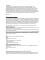
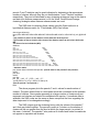
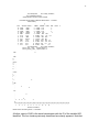
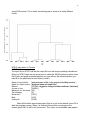
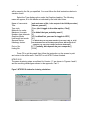
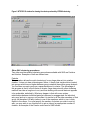
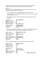
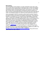
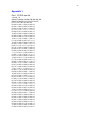
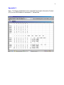
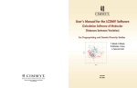
CIMMYT Institutional Multimedia Publications Repository
http://repository.cimmyt.org/
CIMMYT
Genetic Resources
Data analysis in the CIMMYT applied
biotechnology center: For fingerprinting
and genetic diversity studies
Warburton, M.
2002
Downloaded from the CIMMYT Institutional Multimedia Publications Repository
For Fingerprinting and Genetic
Diversity Studies
Marilyn Warburton
and
José Crossa
August 2002
International Maize and Wheat Improvement Center,
Apdo Postal 6-641, CP 06600 México, D.F., México,
http://www.cimmyt.org
Second Edition
1
Table of Contents
I.
Overview……………………………………………………..
2
II.
Data Collection……………………………………………….
2
III.
Data Analysis…………………………………………………
4
Partitioning variation in the sample…………………………
4
Ordination: visualizing the relationships in the samples….
6
Proximity matrices…………………………………….
6
Clustering………………………..……………..………
13
Determining approximate number of clusters using SAS. 13
IV.
Other SAS clustering procedures………………………..
18
Multidimensional scaling………………………………..
20
Principal components analysis………………..………...
20
Interpretation of the Data………………………………………..
22
Bootstrapping……………………………………………
V.
References……………………………………………………….
23
24
Appendix 1: Sample data files…………………………………..
25
Appendix 2: Excel spreadsheet for PIC calculations……………
28
2
I. Overview
The molecular genetic characterization of the diversity present in the CIMMYT maize
and wheat germplasm collections is an ongoing process, to which many different
persons have contributed. Furthermore, one of the mandates of CIMMYT is training
of our national program partners, who have also expressed interest in learning the
statistical techniques we use here at CIMMYT. It may even be possible one day to
combine data from different labs into one analysis. In an effort to standardize the
process and the results, and as a teaching tool for interested parties, this manual
was prepared to act as a set of guidelines for future diversity analyses of maize and
wheat germplasm. The analysis tools will also work in other species.
Three main steps are involved in the statistical analysis of molecular data in
diversity studies: (1) Data collection (scoring and entry of band information into the
computer); (2) Data analysis using Univariate and Multivariate Statistical
approaches; and (3) Interpretation of the data. Each step in the process should
follow a standardized format if the output of one diversity study is to be compared to
other studies and inferences drawn in this manner. Likewise, laboratory procedures
must be standardized between different workers; to achieve this end, all users
should read the manual entitled “Laboratory Protocols: CIMMYT Applied Molecular
Genetics Laboratory,” which should be followed when initiating diversity studies.
This manual will provide both simple examples of all procedures in the main
body of the text and real examples of data analyses in the appendices. Please refer
to these examples when questions arise regarding any procedure mentioned in this
manual.
II. Data Collection
Data used in genetic diversity studies of plant species are molecular markers
(namely, Amplified Fragment Length Polymorphisms, AFLPs; Random Amplified
Polymorphic DNA, or RAPDs; Restriction Fragment Length Polymorphisms, RFLPs;
and Simple Sequence Repeats, or SSRs). RAPD and SSR markers are PCR-based,
and thus avoid the main difficulties associated with RFLP or AFLP data; specifically,
the cost and time involved in isolation of sufficiently high-quality DNA and
visualization of the bands via radioactivity, fluorescence, or bio-luminescence. It
should be cautioned, however, that RAPD bands have demonstrated some problems
related to repeatability. For an overview on molecular markers, we suggest GENES
VII by Lewen (Oxford University Press, 2000) or the Molecular Cloning Laboratory
Manual by Sambrook et al. (2001).
The data can be scored as presence/absence (1 or 0) in the case of dominant
markers (such as RAPDs or AFLPs) or as allele frequencies for SSRs or RFLPs.
SSRs and RFLPs can also be scored as presence/absence, but some genetic
information will be lost, so more markers should be used if markers will be scored
this way. For presence/absence data, the data should be entered into a spreadsheet
(such as EXCEL) in the format followed in Table 1. Rows should correspond to
variables or markers, and columns should correspond to the taxonomic units or lines
3
(cultivars, landraces, etc.) in the study. For the Excel file, name each marker and
cultivar, preferably using names that are less than 8 characters long, and avoid nonalphanumeric characters (such as periods, dashes, etc.).
The example in Table 1 corresponds to data that will be analyzed using SAS.
For NTSYS, all periods (which indicate missing data) should be replaced with 9,
either in the Excel table or later using Word.
Table 1. Example of Excel data file with five different maize lines (corresponding to
columns) and 10 different marker bands (corresponding to rows). 1 = band present,
0 = band absent, . = missing data.
MaizeA
MaizeB
MaizeC
MaizeD
MaizeE
AFLPA1
1
1
1
0
1
AFLPA2
1
1
1
1
1
AFLPB1
0
0
1
0
1
AFLPB2
1
1
0
.
0
AFLPC1
1
0
1
0
0
AFLPC2
1
.
0
0
0
AFLPC3
0
0
1
1
1
AFLPC4
0
0
0
1
1
AFLPC5
0
1
1
1
1
AFLPC6
1
1
1
0
.
When all your data has been entered, check for rows or columns with too
much missing data. Missing data can distort the analyses. You will need to decide
how much is too much; you may wish to run some analyses on the entire data set
and then again on a sub-set of the data after removing the individual lines or markers
that contain a lot of missing data (a good rule of thumb; if more than 15% of the
observations are missing data for any given marker or maize, it is TOO MUCH! For
the entire data set, you want to minimize missing data overall). When you have
removed the individuals or markers with too much missing data, save the file as a
text file without the column labels. For the SAS procedures demonstrated in this
manual, you want the rows to be labeled with the marker name. Do not include
spaces or punctuation, and do not begin the name with a number (although you can
have numbers in the name). Make sure all the names are the same length, or that
you include spaces at the end of the name so that the observations start at the same
column in Word. You will want one space between each observation, and put one
space at the end of each line before the return character. If you do not add this
return, SAS will not accept your data. A SAS input data file example is shown in
Figure 2.
4
Fig. 2. Input data file for SAS, saved as a text file, with 5 different maize lines and 10
different marker bands; this file corresponds to the Excel file shown in Table 1.
AFLPA1
1
1
1
0
1
AFLPA2
1
1
1
1
1
AFLPB1
0
0
1
0
1
AFLPB2
1
1
0
.
0
AFLPC1
1
0
1
0
0
AFLPC2
1
.
0
0
0
AFLPC3
0
0
1
1
1
AFLPC4
0
0
0
1
1
AFLPC5
0
1
1
1
1
AFLPC6
1
1
1
0
.
For NTSYS versions older than 2.02, you must make sure the length of each
line of data does not exceed approximately 45 columns in Word (including spaces),
or the NTSYS program will not read your data properly. A heading must also be
placed at the beginning of the NTSYS data file as follows: 1 10 5 1 9. The numbers
refer to (in order presented here): the type of data matrix (1 = rectangular raw data
matrix, as we have here); 10 = number of rows (markers, or variables); 5 = number
of columns (maize, or entries); 1 = there is missing data (as opposed to 0, which
would mean that there is no missing data in the entire file); and 9 = what we called
the missing data. You can call it any number you like, but NTSYS, unlike SAS, will
not accept a period. An example of an NTSYS input data file can be found in
Appendix 1.
NTSYS version 2.02 has a built-in data editor where you can enter the data
directly, or open an Excel file for import into NTSYS. However, on frequent
occasions, we have had problems with this data editor (it may not recognize our
Excel files, and data entered into the editor cannot be printed nor exported to Excel).
Therefore, we do not routinely use this data editor. More information on the data
editor can be found in the NTSYS manual, version 2.02 or 2.10.
III. Data Analysis
Partitioning variation in the sample
Usually, one of the first steps in a diversity study is to investigate the variation
present in the sample under study (not to visualize relationships between individuals,
but simply to see the overall breakdown of variation in the sample and, if it is a
comparison of populations, the partitioning of diversity within and between
populations. Some tools are available to quantify the variation present and how it is
broken down among individuals, populations, and markers.
A good program for partitioning variation between populations and within
them, and also between and within clusters following a cluster analysis (which will be
discussed later) is the AMOVA (analysis of molecular variation) procedure. This is
very similar to the ANOVA procedure, and is very commonly used, so it will not be
5
discussed in this manual. For a complete review of the AMOVA, see Excoffier et al.
(1992).
One can also measure the richness of alleles for each marker, or the
information that each marker imparts to the study. It can also be looked at as the
measure of usefulness of each marker in distinguishing one individual from another.
Several factors affect this usefulness, including number of alleles, frequency of these
alleles in the study, and others. Three measures of the usefulness of the markers are
allele richness, Polymorphic Information Content, (PIC), and discriminatory power of
the markers. Allele richness is can be calculated in the LCDMV software package by
Dubreuil et al. (2002). This package runs on SAS and can be downloaded from the
CIMMYT webpage at http://www.cimmyt.cgiar.org/ABC/Protocols/manualABC.html,
along with the user’s manual and source code, if desired. A discussion of the
calculation of discriminatory power of marker can be found in Franco et al. (2001).
An example of calculating PIC is presented here.
PIC is a quantification of the number of alleles or bands that a marker has and
the frequency of each of the alleles or bands in the population of OTUs in the study.
Since a marker with fewer bands has less power to distinguish several OTUs, and
alleles present at low frequency also have less power to distinguish, a higher PIC is
assigned to a marker with many alleles and with alleles present at roughly equal
proportions in the population. We use an Excel spreadsheet to calculate PIC, a copy
of which is found in Appendix 2. Remember, when using Appendix 2, several of the
cells contain equations and not numbers, (see Part 2 to see the formulas), so you will
have to adjust the equations depending on the source cells that the equations are
using as data.
The formula used to calculate PIC is:
PIC = 1 - Σpi2
Where pi is the frequency of the ith allele for individual p.
To use the excel spreadsheet, perform the following steps:
Step 1: Enter the data as presence (1) or absence (0) of each allele (in rows) for
each OTU (in columns).
Step 2: Change the 1 in each cell to a 2 if the OTU is homozygous for that allele;
leave it as a 1 if it is heterozygous and there is another allele present for that SSR in
that OTU. You can sum over all alleles for each SSR to make sure the sum is 2 in
every individual for every SSR; in this way, you know that you have not misscored
any individuals, as every individual will have two alleles for every SSR.
Step 3: Sum alleles over OTUs.
6
Step 4: Divide the sum by the total number of alleles possible at each locus to get
the frequency of occurrence of each allele (in this case, with 7 OTUs of diploid
individuals, you have 14 possible alleles, so divide by 14). Frequencies must sum to
1.
Step 5: Square the frequency of each allele.
Step 6: Sum the squared frequencies.
Step 7: Subtract the summed squared frequencies from 1.
Ordination; visualizing relationships in the sample
The classification and/or ordination analyses performed on molecular data all use a
dissimilarity or similarity matrix as input files. This section will be divided according to
the procedures, and will begin with the calculation of similarity matrices. Please see
the SAS or the NTSYS manuals for further explanation of any of the procedures
listed here. A good overview of the theory can be found in Beaumont et al. (1998).
Proximity matrices
For AFLP data (and other dominant marker systems), we will calculate the similarity
(or dissimilarity, the two together known as Proximity) between individuals using the
methods for calculating diversity based on qualitative differences. Direct calculation
of genetic distance is possible only for co-dominant marker data where it is possible
to calculate allelic frequencies for each marker in a population. This will be
demonstrated in the following section. With dominant marker data, this is impossible
since the heterozygous individuals cannot be distinguished from the dominant
homozygous individuals, thus making it impossible to calculate the exact frequency
of the dominant vs. recessive alleles. In cluster analysis, many different proximity
measurements can be used. In this manual, we use the Simple Matching, Jaccard’s
(= Gower’s is Jaccard), and Dice (= Nei and Li) coefficients for calculating the
phenotypic distance between each pair of entries (maize lines) in the diversity study.
These are the three most commonly used coefficients in the literature. Other
coefficients can easily be calculated by consulting the NTSYS manual; other
coefficients calculated by SAS require more work as SAS is not as user-friendly as
NTSYS. One final note: the SAS procedures listed here calculate dissimilarity, rather
than similarity, matrices, but this turns out simply to be = 1-similarity, and the
resulting dendrograms and scatter plots are identical for either one. The SAS
procedure PROC CLUSTER that we will examine later always uses dissimilarity
(distances) measurements.
SAS calculation of Dissimilarity Matrices
The following is a SAS code (called Alldist.sas) that can be used to calculate the
proximity coefficients Simple Matching, Jaccard’s (= Gower’s) and Dice (= Nei and
Li, 1979) coefficients. Parts in bold italics are notes, and not part of the protocol; do
7
not include them in the SAS program. The notes tell you which part of the program
must be changed according to the data set.
OPTIONS LINESIZE = 132 PAGESIZE = 77;%MACRO DISSIMLR;%LET N=35; (change the 35 to the
number of lines, or maize, you have)
%DO I=1 %TO &N;
DATA A;
INFILE 'C:\DATA\allpoly.PRN' LRECL=340 (change the file path and name inside the quotes to your
file and the correct path)
(change the 340 to a larger number if your data set has a lot of individuals, make it about 10 x the number
of lines you have)
FIRSTOBS=1;
INPUT BAND $ 1-8 @9 (SUBJ1-SUBJ&N) (2.); (change the 1-8 to the number of spaces that your
marker labels take up in your data set; for example, in Fig 2, the marker labels take up spaces 1 – 7.
Change the @9 to the next space after your markers; for example in Fig 2, it would be @8)
ARRAY SUBJ(&N) SUBJ1-SUBJ&N;
ARRAY NUM(&N) NUM1-NUM&N;
ARRAY DEN(&N) DEN1-DEN&N;
ARRAY DIST(&N) DIST1-DIST&N;
ASSOC=3; (choose Assoc=1 for Gower’s (Jaccard’s) coefficient; Assoc=2 for Nei and Li (Dice), and
Assoc=3 for Simple Matching (default)).
DISTNC=1;
IF ASSOC=1 THEN
DO J=1 TO &N;
IF SUBJ(&I)=1 AND SUBJ(J)=1 THEN N=1;
ELSE N=0;
IF SUBJ(&I)=0 AND SUBJ(J)=0 THEN D=0;
ELSE IF SUBJ(&I)=. OR SUBJ(J)=. THEN D=0;
ELSE D=1;
NUM(J) + N;
DEN(J) + D;
END;
IF ASSOC=2 THEN
DO J=1 TO &N;
IF SUBJ(&I)=1 AND SUBJ(J)=1 THEN N=2;
ELSE N=0;
IF SUBJ(&I)=1 AND SUBJ(J)=1 THEN D=2;
ELSE IF SUBJ(&I)=0 AND SUBJ(J)=0 THEN D=0;
ELSE IF SUBJ(&I)=. OR SUBJ(J)=. THEN D=0;
ELSE D=1;
NUM(J) + N;
DEN(J) + D;
END;
IF ASSOC=3 THEN
DO J=1 TO &N;
IF SUBJ(&I)=1 AND SUBJ(J)=1 THEN N=1;
ELSE IF SUBJ(&I)=0 AND SUBJ(J)=0 THEN N=1;
ELSE N=0;
IF SUBJ(&I)=. OR SUBJ(J)=. THEN D=0;
ELSE D=1;
NUM(J) + N;
DEN(J) + D;
END;
IF BAND='S9D' THEN (write the name of your last band in your data set; for example in fig 2 it would
say IF BAND=’AFLPC6’)
IF DISTNC=1 THEN
8
DO J=1 TO &N;
DIST(J)= SQRT(1-(NUM(J)/DEN(J)));
END;
IF DISTNC=2 THEN
DO J=1 TO &N;
DIST(J)= 1-(NUM(J)/DEN(J));
END;
RUN;
DATA B;
SET A (KEEP=DIST1-DIST&N FIRSTOBS=281); (281 refers to number of markers you have; change
this value accordingly)
FILE 'C:\DATA\allpoly.MTX' LRECL=1030 MOD; (change the filename between the quotes to a name
you choose for the output of the analysis, including the path)
PUT (DIST1-DIST&N) (7.4);
RUN;
%END;
%MEND;
%DISSIMLR;
To input this file into SAS, open the SAS program and open a file by using the
file menu. The opened file will appear in the Program Editor window. Submit the
program by clicking on the button that looks like a little man running. Text will appear
in the Log box; if there are errors the text will be red; if there are no errors, the text
will all be blue and black. The output, a square matrix, which is the same above the
diagonal as below, will be saved in the file you specified. The diagonal will be 0,
since it is the comparison of an individual with itself, and cannot be similar. Note: If
you run the same procedure more than once, erase the old output file before you
start, or name it something different, because SAS appends the new data file to the
end of the old one, rather than overwriting it.
SAS cannot use the output of this program directly for the other programs that
are listed below; it must first be modified by adding the name of each maize line into
the file at the beginning of each line. You can do this in Word; remember that the
labels must all be the same length, or have the same number of spaces following
each one until they all have the same number of characters + spaces. Save the file
as text because the output of this program will be used directly for cluster analysis,
principal components, etc. You can also use Excel to insert one column with the
labels, but you must save it as a text file with a space between each column and a
space at the end of each row (which must still be done in Word).
NTSYS calculation of Similarity Matrices
Dominant marker types:
NTSYS 1.7
The input file for NTSYS will be similar to the SAS input file but with a few
exceptions; see Appendix 1 for more details. You will not need to write a program to
tell NTSYS what to do, since it is a menu-driven program. Simply enter into NTSYS
and use the arrow keys to move around the menu. Select the Qualitative option
9
under the (Dis)Similarity Measures heading, and you will see the following screen:
(you must fill in the parts listed in bold italics yourself)
Name of input matrix:
Coefficient:
Name for output matrix:
By rows or cols?
Positive code
Negative code
Show matrix?
Listing file
[ path and name of file ]
[ SM is default; press space bar to toggle to other options]
[ path and name of output file ]
[ COL is default but we need ROW; press space bar to
change]
[1]
[0]
[ NO ]
[ CON ]
When all the blank spaces have been filled in or left as the default, press F2 to
start the program running. When it is finished (there will be a message on the
screen) press ESC to exit to the main menu. Press ESC again to exit NTSYS when
you are finished. The output, a diagonal matrix, will be saved in the file you specified
(only one half is displayed; unlike SAS it does not print both above and below the
diagonal). The diagonal will be 1, since it is the comparison of an individual with
itself, and cannot be dissimilar.
NTSYS 2.02 and 2.1
NTSYS 2.02 has all the same options and calculations as NTSYS 1.7, but the menus
have been updated to Windows. Instead of moving around the menus with the arrow
keys, you can click on the window you want and then on the option you want. For
Similarity calculations, you click on the Similarity heading, then chose SimGen (for
allele frequency data) or SimQual (for zero and one data). See Figure 3 for an
example of calculation of Simple Matching coefficients. Note: NTSYS 2.02 and 2.1
have an online help menu which can be accessed by clicking the Help Option from
the main task bar.
10
Figure 3. NTSYS 2.1 window for calculating Simple Matching similarity coefficients.
Co-dominant marker types
NTSYS 2.02 and 2.1
When allelic relationships between bands are known (as in the case of RFLPs and
SSRs), genetic distances can be calculated between individuals in a study.
Distances such as Nei and Li (1979) and Roger’s (1972) or Modified Roger’s are
examples of this type of distance. An NTSYS 2.1 example of Nei and Li distance
calculation will be shown here. NTSYS also calculates Roger’s distances, but an
error in the program causes the calculations to be incorrect, so a SAS or other
program procedure should be used for this instead.
The following example is taken from the NTSYS 2.1 online help manual.
Matrices for gene frequency data must contain the frequencies of all the alleles (i.e.,
the frequencies must add up to 1 for each locus. In the example shown below, the 19
rows correspond to 19 alleles distributed over the 5 loci. The columns correspond to
11
samples taken from four populations. The first 4 rows correspond to the alleles at the
ABO locus. Thus the column sums must be equal to 1 for the first 4 rows. The next
five rows correspond the next locus within which the columns must sum to 1, and so
on for the remaining loci. The following example input file will be used in the example
in Figure 4. More than one space is allowed between observations in this version of
NTSYS. Note the two comment lines at the beginning of the file (starting with “)
" Blood-group data from Cavalli-Sforza and Edwards (1967)
" 5 loci with a total of 19 alleles for 4 populations
1 19L 4L 0
A1 A2 B O CDE CDe cDE cDe Cde cdE cde MS Ms NS Ns Fya Fyb
Dia Dib
Eskimo Bantu English Korean
0.2914 0.1034 0.2090 0.2208
0
0.0866 0.0696 0
0.0316 0.1200 0.0612 0.2069
0.6770 0.6900 0.6602 0.5723
0
0
0.0024 0.0082
0.4985 0.1400 0.4205 0.6197
0.4906 0.0100 0.1411 0.3148
0.0109 0.6000 0.0257 0.0573
0
0.0200 0.0098 0
0
0
0.0119 0
0
0.2300 0.3886 0
0.1719 0.0900 0.2377 0.0245
0.6703 0.4800 0.3048 0.4615
0
0.0400 0.0703 0.0646
0.1578 0.3900 0.3872 0.4494
0.7500 0.0600 0.4213 0.9950
0.2500 0.9400 0.5787 0.0050
0
0
0
0.0313
1
1
1
0.9687
For some coefficients the SIMGEND module needs to know which alleles
correspond to the same locus. This information is provided in a rectangular matrix
(stored in a separate file) that contains a single row (or column) of codes indicating
the locus that each allele belongs to. This information can also be used by the FREQ
module. An example is shown below for the above data.
" Loci info for
" Blood-group data from Cavalli-Sforza and Edwards (1967)
1 1 19L 0
A1 A2 B O CDE CDe cDE cDe Cde cdE cde MS Ms NS Ns Fya Fyb
Dia Dib
1111 2222222 3333 44 55
12
For some coefficients, the SIMGEND module needs to know the sample size
for each population being compared. A rectangular matrix with a single row or
column provides this information. This matrix can be produced by the FREQ module.
An example is given below.
" sample size matrix for 4 populations
1140
25 25 25 25
© 2000 by Applied Biostatistics, Inc.
Figure 4. NTSYS 2.1 window for calculating Nei’s 1972 genetic distance coefficients.
13
Clustering
The first type of clustering we will perform on the proximity matrices is the
Unweighted Pair Group Method using Arithmetic Averages UPGMA). This is a
hierarchical algorithm for clustering entries (maize) into similar groups. For a more
detailed description of the algorithm used to calculate the dendrogram, see the
NTSYS or SAS manuals. The output of this clustering procedure is a dendrogram or
tree with distance along the horizontal (top) axis and the maize lines listed vertically
down the side (see Fig. 4 as an example; more output trees can be found in
Appendix 1).
SAS calculation of clusters
The following is a SAS code (called Cluster.sas), which can be used to calculate the
dendrogram for the UPGMA, Ward, or Single Linkage methods. Parts in bold italics
are notes, and not part of the protocol; do not include them in the SAS program. The
notes tell you which part of the program must be changed according to the data set.
Note that version 8.00 of SAS calculates the dendrogram automatically so that this
SAS codes are only needed if you use any SAS version prior to version 8.00.
OPTIONS LINESIZE = 132 PAGESIZE = 77;Title 'Cluster Analysis of GBG experimental lines';
(change title inside of quotes)
data DIST(type=distance);
INFILE 'a:\usedata.txt' LRECL=1050; (change the file path and name inside the quotes to your file and
the correct path; use the output of mergcult.sas)
INPUT LINE $ 1-12 @13 DIST1-DIST93; (the numbers refer to columns; be sure these numbers agree
with the numbers in Alldist.sas)
PROC CLUSTER DATA=DIST METHOD=AVERAGE OUTTREE=TREE; (choose METHOD=AVERAGE
for UPGMA (default); METHOD=WARD for Ward’s, and METHOD=SINGLE for single linkage calculations)
ID LINE; VAR DIST1-DIST93; (the numbers refer to number of markers; be sure these numbers agree
with the numbers in Alldist.sas)
RUN;
PROC TREE DATA=TREE HORIZONTAL SPACES=2;
ID LINE;
RUN;
GOPTIONS HSIZE=6. VSIZE=8.;
TITLE ;
* BRING THE MACRO INTO THE PROGRAM;
*%INCLUDE DENDRO;
*%DENDRO(FORMAT=LANDSCAPE);
*RUN;
* BRING THE MACRO INTO THE PROGRAM;
%INCLUDE GRFTREE/NOSOURCE2;
%GRFTREE(CLUSDSN=TREE,ITEMS=93,AXIS=D,LABEL=Genetic (set ITEMS=number of maize
lines you have)
Dissimilarity,FONT=SIMPLEX);
RUN;
Determining the approximate number of clusters using SAS
A question always raised following cluster analysis is: What grouping are the “real”
clusters, and at what level of proximity must I draw the line to determine this? The
14
pseudo F and t2 statistics may be good indicators for determining the approximate
number of clusters although they are not distributed as F and t2 random variables,
respectively. They can be calculated for any clustering strategy as long as the data is
raw data (not distance measurements) or for the Ward, Centroid and Average
clustering strategies when distance measurements are used.
The SAS code for obtaining these values using the Ward method in a
hypothetical distance matrix for 13 individuals (IND) is as follows.
data a (type=distance);
input (IND1 IND2 IND3 IND4 IND5 IND6 IND7 IND8 IND9 IND10 IND11 IND12 IND13) (4.2) @78 IND
$6.;
* (4.2) number of places for the distance values with two decimal places;
* @78 number of places from the left column of the distance matrix to the column before the
IND;
* $6. Places for the individuals (IND);
datalines;
0.00
0.99
0.98
0.55
0.77
0.46
0.50
0.87
0.30
0.25
0.55
0.45
0.46
0.00
0.53
0.21
0.30
0.24
0.41
0.35
0.90
0.80
0.70
0.60
0.68
0.00
0.27
0.92
0.42
0.67
0.81
0.50
0.40
0.90
0.80
0.81
0.00
0.72
0.92
0.18
0.39
0.34
0.14
0.84
0.74
0.70
0.00
0.98
0.87
0.30
0.89
0.09
0.99
0.89
0.85
0.00
0.39
0.75
0.12
0.92
0.92
0.82
0.81
0.00
0.45
0.34
0.44
0.54
0.44
0.43
0.00
0.23
0.13
0.53
0.43
0.44
0.00
0.21
0.31
0.21
0.20
IND1
IND2
IND3
IND4
IND5
IND6
IND7
IND8
IND9
0.00
IND10
0.34 0.00
IND11
0.24 0.23 0.00
IND12
0.25 0.25 0.28 0.00 IND13
; *distance matrix;
proc cluster data=a method=ward pseudo; *pseudo asks for the pseudo F and pseudo t;
id IND;
proc tree;
id IND;
proc plot;
plot _psf_*_NCL_='F' _PST2_*_NCL_='T'/
overlay haxis=1 to 13 by 1 vaxis=0 to 300 by 50;
*Plot the pseudo F and pseudo t;
RUN;
The above program plots the pseudo F and t2 values for each number of
clusters. The place where there is a local peak should be considered as the possible
number of clusters. Some peaks appearing at a larger number of clusters may not
represent real clusters and should be considered with caution. If coordinate data is
available, the SAS codes are the same as these except that the lines regarding the
data steps need to be changed accordingly.
The SAS outputs give the clustering history with the values of the pseudo F
and t that are plotted together. The pseudo t peaks at 3 clusters so the number of
clusters will be one greater than the level at which the large pseudo t is printed (in
this case, 4 clusters). The pseudo F also peaks at 4 clusters and further increases do
not appear to represent real clusters.
15
The SAS System
14:51 Friday, October 6,
The CLUSTER Procedure
Ward's Minimum Variance Cluster Analysis
Root-Mean-Square Distance Between Observations = 0.532831
Cluster History
T
i
NCL --Clusters Joined--FREQ SPRSQ RSQ PSF PST2
12 IND2
IND3
2 0.0000 1.00
.
. T
11 IND5
IND6
2 0.0000 1.00
.
. T
10 IND8
IND9
2 0.0000 1.00
.
. T
9 IND11
IND12
2 0.0000 1.00
.
. T
8 IND7
IND10
2 0.0024 .998 300
.
7 CL11
CL8
4 0.0064 .991 112 5.4
6 CL12
IND4
3 0.0086 .983 78.8
.
5 CL9
IND13
3 0.0379 .945 34.1
.
4 IND1
CL5
4 0.0957 .849 16.9 5.1
3 CL7
CL10
6 0.1924 .657 9.6 87.2
2 CL6
CL3
9 0.2159 .441 8.7 7.2
1 CL4
CL2
13 0.4407 .000
.
8.7
The SAS System
14:51 Friday, October 6,
Plot of _PSF_*_NCL_. Symbol used is 'F'.
Plot of _PST2_*_NCL_. Symbol used is 'T'.
e
300 ˆ
F
‚
‚
250 ˆ
P ‚
s ‚
e 200 ˆ
u ‚
d ‚
o ‚
‚
F ‚
‚
S 150 ˆ
t ‚
a ‚
t ‚
i ‚
s ‚
F
t ‚
i 100 ˆ
c ‚
‚
T
‚
F
‚
50 ˆ
‚
‚
F
‚
‚
‚
F
‚ T
F
F
T
T
0ˆ
Šƒƒˆƒƒƒƒƒƒˆƒƒƒƒƒƒˆƒƒƒƒƒƒˆƒƒƒƒƒƒˆƒƒƒƒƒƒˆƒƒƒƒƒƒˆƒƒƒƒƒƒˆƒƒƒƒƒƒˆƒƒƒƒƒƒˆƒƒƒƒƒƒˆƒƒƒƒƒƒ
1
2
3
4
5
6
7
8
9 10 11 12
Number of Clusters
NOTE: 38 obs had missing values. 1 obs hidden.
A further output of SAS is the actual dendrogram with the ID of the variable IND
identified. The four clusters previously determined are clearly apparent. Note that
16
using SAS version 6.12 or earlier the dendrogram is shown in a totally different
format.
NTSYS calculation of Clusters
NTSYS 1.7
The input file for NTSYS will be the output file from the simple matching calculations.
Enter into NTSYS and use the arrow keys to select the SAHN clustering option under
the Cluster and graph methods heading, and you will see the following screen (you
must fill in the parts listed in bold italics yourself):
Name of input matrix:
Name for output matrix:
Method
In case of ties
Maximum no. tied trees
Tie tolerance
Show tree?
Beta
Listing file
[ path and name of file; is the output of the SM procedure ]
[ path and name of output file ]
[ UPGMA toggle to change to other methods, if desired]
[ WARN ]
[ 25 ]
[0]
[ YES ]
[-0.25]
[ CON ]
When all the blank spaces have been filled in or left as the default, press F2 to
start the program running. When it is finished (there will be a message on the
screen) press ESC to exit to the main menu. The output, an unreadable tree graphic,
17
will be saved in the file you specified. You must follow the final instructions below to
visualize it well.
Select the Tree display option under the Graphics heading. The following
menu will appear; fill in the blanks as indicated by the bold italic notes:
Name of tree matrix:
Title:
Tree style
Minimum for scale:
Maximum for scale:
Number class intervals:
Graphics Mode:
Line length text mode:
Squeeze factor:
Hardcopy device:
Port or file:
Listing file:
[ path and name of file; is the output of the SAHN procedure ]
[ choose yourself ]
[ Phen (don’t toggle to the other option, Clad) ]
[0]
[ 0 is default but you probably want 1 ]
[0]
[ NO is default but you need to toggle to YES ]
[ 61 ]
[1 is default but you may want smaller if your tree is big, ie, 0.75]
[use the down arrow to find the proper printer; HP laserjet II, for
example; you can print in either portrait or landscape]
[LPT1 (usually, but depends on your computer) ]
[ CON ]
Press F2 to get the graph, then follow the instruction on the screen to print
and return to the main menu. Use ESC to exit NTSYS when finished.
NTSYS 2.02
The same clustering steps as outlined for Version 1.7 are shown in Figures 4 and 5,
and the resulting dendrogram shown in the appendix, Part 3.
Figure 5. NTSYS 2.02 window for clustering calculations.
18
Figure 6. NTSYS 2.02 window for drawing the cluster produced by UPGMA clustering.
Other SAS clustering procedures
Two other non-hierarchical clustering procedures available with SAS are Fastclus
and Varclus. Examples of both are shown here.
Fastclus
This procedure allows the quick clustering of a very large data set into putative
clusters. It does not draw a dendrogram; rather, it simply lists similar entries (maize)
into groups which have a higher between-group variance then within-group variance.
You can then use each group as a separate data set to cluster. The advantage of
this program is that it is much faster to cluster (large data sets with other clustering
methods can take a long time to run) and that working with a small data set appears
to be preferable, statistically. What may happen is that with more entries,
relationships between individual pairs get obscured or exaggerated. An individual
entry may end up in a group, not because it is similar to all the other members of that
group, but because it is fairly similar to one of the members, which in turn is fairly
similar to the others. You must specify the number of clusters you wish to end up
with; you may wish to run Varclus first to get an idea of an appropriate number of
clusters. An example of the Fasclus code used in SAS follows:
19
OPTIONS LINESIZE = 132 PAGESIZE = 77;Title 'FASTClus Analysis of 123 lines using 35 core
primers'; (change title as appropriate)
data DIST;INFILE 'C:\DATA\core114b.MTX' LRECL=1050; (change the file path and name inside the
quotes to your file and the correct path; use the output of mergcult.sas)
INPUT LINE $ 1-11 @12 dist1-dist35;
PROC FASTCLUS DATA=dist MAXITER=10 DRIFT
LEAST=2 MAXC=25 OUT=out2 SUMMARY REPLACE=FULL LIST;
(Maxc = the maximum number of
clusters you want SAS to use)
ID line; VAR dist1-dist35;
run;
Varclus
Varclus clusters entries (maize) into varying numbers of clusters as specified by the
user; usually starting with two and proceeding to a larger number (not to exceed the
number of entries in the test). This program will tell you when splitting clusters into
smaller groups (and thus a larger number of clusters) does not make statistical
sense; you can, however, choose to use a smaller number of clusters. An example of
the Varclus procedure is shown below:
OPTIONS LINESIZE = 132 PAGESIZE = 77;Title 'VARClus Analysis of GBG ancestors 4-2-98';
(change title as appropriate)
data DIST;infile 'a:\ancestors.txt' (name and path of your input file. NOTE: this is an original data file
NOT the output of Mergclus.sas, therefore you need labels (below))
LRECL=1050;
INPUT band $ 1-6 @7 P68600 P189930 P261474 P290116A P291306A
P297500 P297544 P317335 P347560 P361067 P372415A P378664 P383276
P384469A P384471 P391594 P393999 P398763 P404157 P404161 P404188A
P404192C P407654 P423950 P424159 P437909B P87588 P890612 P91091
P189930A P253665D P283331 P436682 P436684 P437697 P437851A P438206
P69507 P84657 P88310 P189893 P200485 P361006A P361075 P399016
P417510 P427088B P437578 P445837 P467307 P476352C P491548 P491579
P503338 P506920 P506945 P507295 P507296 P507373 P507543 PFC3571
P890612A P227328 P391583 P391584 P424159B P458511 P464878 P464887
P464920 P468377 P475814 LG852534 LG871991 LG921128 LG924208 LG937604
LG937654 LG941309 A3205 S4230 CNS
ILLINI MANDARIN LINCOLN
DUNFIELD RICHLAND AKHARROW ARKSOY CAPITAL HABERLAN JACKSON KOREAN
MUKDEN OGDEN PERRY RALSOY ROANOKE S100;
proc corr data=dist noprint cov outp=covout;
*proc print;
data cov(type=cov);
set covout;
proc varclus data=cov maxeigen=1 initial=random short
maxiter=100 maxsearch=100 ;
run;
20
Multidimensional scaling
This is a procedure for plotting the lines on a graph of two axes for the purpose of
visualizing the relationships between entries and clusters. An example of a SAS
MDS procedure is listed below.
OPTIONS LINESIZE = 132 PAGESIZE = 77;Title 'Cluster Analysis of US and Chinese Ancestors
using only polmorphic data'; (change to appropriate title)
data DIST(type=distance);
INFILE 'C:\DATA\uscnf3.lab' LRECL=1050;
INPUT LINE $ 1-21 @22 dist1-dist35;
PROC MDS DATA=DIST LEVEL=ABSOLUTE DIM=22 OUT=OUT PINEIGVAL PININ
PINIT OUTRES=RES; (set dim= number of dimensions you want. Final R value printed on last page of
SAS output should be at least .95, which means you have accounted for 95% of your original variation in
your analysis. If you set this number too high, it will take a LONG time to run the procedure. As it is, it
takes several hours.)
ID LINE;
PROC PRINT DATA=OUT;
PROC PRINT DATA=RES;
PROC PLOT DATA=OUT VTOH=2.0;
PLOT DIM2*DIM1='*' $ LINE /HAXIS=BY 0.1 VAXIS=BY 0.1;
WHERE _TYPE_='CONFIG';
PROC PLOT DATA=RES VTOH=2.0;
PLOT FITDATA*FITDIST /HAXIS=BY 0.1 VAXIS=BY 0.1;
PROC PLOT DATA=RES VTOH=2.0;
PLOT DATA*DISTance /HAXIS=BY 0.1 VAXIS=BY 0.1;
run;
PROC REG DATA=RES;
MODEL FITDATA=FITDIST;
PROC REG DATA=RES;
MODEL DATA=DISTance;
RUN;
DATA Z;
SET RES;
FILE 'C:\DATA\mdsoutput.PRN' LRECL=1200 MOD; (the output will be VERY big; be sure to put it
somewhere you have enough room!)
PUT LINE 1-21 @22 (DIM1-DIM22) (9.4); (If you change dim=22 to a different number above, be sure to
change it here, too)
RUN;
Principal components analysis
Principal Components is an ordination technique that allows the projection of the
data onto two or three axes in order to visualize the differences in the individuals and
look for groups. The principal components are the new uncorrelated variables that
are calculated from the original variables that may not have a biological meaning
(especially with molecular markers). However, they are a useful since the first two or
three usually account for most of the variation of all the original variables. Whereas it
would be impossible to project the data onto a graph with axes corresponding to all
the variables (usually more than 100 in the case of molecular markers), using PCA
you can project the data onto two or three axes. In three dimensions, you can see
patterns that cannot be represented in a two-dimensional dendrogram. In order to
use PCA, you must first calculate eigenvalues, which represent the amount of
21
variance accounted for by a component, and the eigenvectors, which are the
correlation between the original variable and the principal component.
NTSYS 1.7
Performing PCA using NTSYS requires the following steps (to use SAS for this
procedure, please consult the SAS manual).
1. Convert original data file (c:inputdatamatrix.dat) to a similarity matrix
(c:simmatrix.dat) but run by ROWS (variables) not columns (see section entitled
“Similarity Matrices,” above).
2. Run the eigen program on the similarity matrix to generate eigenvectors and
eigenvalues:
Input Matrix:
[C:simmatrix.dat]
Number of dimensions:
[3]
Sample size of mx:
[0]
Degrees of freedom of mx: [0]
Eigenvector matrix:
[C:simmatrix.vec]
Eigenvalue matrix:
[C:simmatrix.val]
Vector scaling:
[SQRT(LAMBDA)]
Listing file:
[CON]
3. Run the projection program (PROJ) on the matrices to project the transformed
data matrix onto the first three principal components (eigenvectors)
Name of matrix:
[C:intupdatamatrix.dat]
OTUs = rows or cols:
[COL]
Name of factor matrix:
[C:simmatrix.vec]
Projection type:
[Proj]
Name of eigenvalue mx: [C:simmatrix.val]
Name for projection matrix:[C:simmatrix.pro]
Show matrix?
[NO]
Listing file:
[CON]
4. Use the MOD3D program to generate the graph of the output of PROJ.
Name of matrix:
Direction to plot by:
Variable for x-axis:
Variable for y-axis:
Variable for z-axis:
Graph matrix:
Title:
Rotation around z-axis:
Rotation around x-axis:
Viewing distance:
[C:simmatrix.pro]
[ROW]
[1]
[2]
[3]
[ leave blank!!! ]
[choose your title]
[30]
[30]
[99]
_
|
|
|
all these things can be
22
Label the points:
Show the pins:
Show edges in graph:
Normalize scales:
Hardcopy device:
Port of file:
Graphics paging:
Listing device:
[NO]
>
changed while viewing
[YES]
|
graph produced
[YES]
|
[NO]
|
[ choose your printer from list ]
[lpt1 or whatever your printer port is]
[YES]
[CON]
NTSYS 2.02
This version of NTSYS apparently has a problem calculating PCA, and we have not
been able to successfully use 2.02 for this purpose. Therefore, we only use NTSYS
2.1.
IV. Interpretation of the Data
When you have completed clustering using a number of different procedures, you
can compare the outputs to search for “consensus clusters.” Many clusters contain
the same individuals regardless of the clustering algorithm used; you can be fairly
sure in these cases that the clusters represent genetic, biological, or geographical
factors and are a useful classification of the maize lines. However, some lines will
show up in a different cluster each time a different clustering procedure is used.
These lines are more difficult to assign to their “proper” cluster, and you may need to
assign them to the cluster that makes the most sense based on known pedigree,
region of origin, etc. However, this is cheating a little; you are forming a hypothesis
(which group does a particular line belong to?) and testing it with the same data
when you do this; this is statistically shaky. Also, if you have no prior data on a given
line, you may not be able to place it into any cluster; thus you may not be able to
include this line in the analysis. In all cases, be sure to explain why each individual
was placed in the cluster you finally decide to put it in.
Using NTSYS, you can compare the matrix produced by the SAHN procedure
with the similarity coefficient matrix using the MXCOMP procedure; if there is a good
correlation (above 0.9, for example) you can be more certain that the dendrogram
produced is a good representation of the data (see NTSYS manual for instructions).
Finally, in order to visualize the data, you may wish to present the MDS or PCA
graph, which gives a good three-dimensional picture of the variation. You can group
the consensus clusters by drawing circles around individuals or coloring them the
same color.
23
Bootstrapping
One final method for testing whether your data is statistically sound, and to make
sure you have used enough markers in analyzing the data, is called “bootstrapping.”
This method involves repeated analysis of the same data set to see if the resulting
dendrograms change a lot following each analysis. If the program is unsure of the
data, or if there are not enough markers, the algorithms used for clustering may
result in clusters containing individuals that do not fit particularly well in that particular
cluster. A bootstrapping program can repeat the cluster analysis many times and
return a dendrogram in which the clusters are defined by the number of times the
individuals within the cluster were found together in each analysis. This number can
be used as a confidence limit of the clusters within the dendrograms (Felsenstein,
1985). To ensure that the accuracy of the bootstrap is 95%, 400 repetitions of the
analysis must be done, and 2,000 repetitions must be done to ensure the accuracy is
99% (Hedges, 1992). We recommend the WinBoot program by Yap and Nelson
(1996) as a user friendly, free program for performing bootstrap analysis of binary
data to determine the confidence limits of UPGMA-based dendrograms. However,
this program only does UPGMA, and does not accept missing data in the data
matrix. The authors may be contacted via the Internet at the following email
addresses: [email protected] (for technical support) and r.nelson @cgnet.com (for
distribution/general inquiries. For other dendrograms or data types, SAS routines
have been calculated in the LCDMV software package by Dubreuil et al. (2002). This
package can be downloaded from the CIMMYT webpage at
http://www.cimmyt.cgiar.org/ABC/Protocols/manualABC.html, along with the user’s
manual and source code, if desired.
24
V. References
Beaumont, M.A., K. M. Ibrahim, P. Boursot, and M. W. Bruford. 1998. Measuring
genetic distance. P. 315-325. In; A. Karp, P.G. Isaac, and D. S. Ingram (ed.)
Molecular tools for screening biodiversity. London: Chapman and Hall.
Dubreuil, P., C. Dillman, J. Crossa, and M. Warburton. 2002. LCCMV: Software for
the Calculation of Molecular Distances between Varieties. First Edition.
Mexico, D.F.: CIMMYT.
Excoffier, L., P. Smouse, and J. Quattro. 1992. Analysis of molecular variance
inferred for metric distances among DNA haplotypes: application to human
mitochondrial DNA restriction data. Genetics 131:479-491.
Felsenstein J. 1985. Confidence limits of phylogenies: an approach using the
bootstrap. Evolution 39:783-791.
Franco, J., J. Crossa, J.M. Ribaut, J. Betran, M.L. Warburton, and M. Khairallah.
2001. A method for combining molecular markers and phenotypic attributes
for classifying plant genotypes. TAG, 103(6/7):944-952.
Hedges SV. 1992. The number of replications needed for accurate estimation of the
bootstrap P value in phylogenetic studies. Mol. Biol. Evol. 9:366-369.
Hoisington, D., M. Khairallah, and D. Gonzalez-de-Leon. 2000. Laboratory Protocols:
CIMMYT Applied Molecular Genetics Laboratory. Third Edition. Mexico,
D.F.:CIMMYT
Lewin, Benjamin. 2000. Genes VII. Oxford University Press.
Nei, M. and W. Li 1979. Mathematical model for studying genetic variation in terms of
restriction endonucleases. Proc. Natl. Acad. Sci. (USA) 76:5269-5273.
NTSYSpc 2.10. 2000. Applied Biostatistics, Inc.
Rohlf, F.J. 1997. NTSYSpc: Numerical Taxonomy and Multivariate Analysis System,
version 201. Department of Ecology and Evolution, State University of New
York.
Sambrook, J., D. Russell, and J. Sambrook. 2001. Molecular Cloning: A Laboratory
Manual 4th ed. Cold Spring Harbor Laboratory.
SAS/STAT, User’s Guide, Version 6, Fourth Edition. SAS Institute Inc.: Cary, NC.
Yap I., and R.J. Nelson. 1996. WinBoot: a program for performing bootstrap analysis
of binary data to determine the confidence limits of UPGMA-based
dendrograms. IRRI. Discussion Paper Series No. 14. International Rice
Research Institute, P.O. Box 933, Manila, Philippines.
25
Appendix 1.
Part 1. NTSYS data file.
1 48 19L 1 9
CML247 CML254 CML258 CML264 CML268
CML273 CML274 LP1 LP2 LP3 LP4 LP5
P1 P21 TS1 TS2 TS3 TS4 TS5
0000000010000000000
0000100000000000000
0000000000001000000
0111011011111111101
0000000100000000010
1000000000000000000
0000900901000000000
0000900900110000000
1001911910000110010
0110900900001001101
1000000000000000000
0000010001000010110
0001011010111001001
0010100000000000000
0000000100000100000
0000000000001000000
1111000101100000001
0100111010010111111
0001000000000000000
1000000101110000000
0110000000000000110
0000100000001011001
0000011010000100000
0001000000000000000
0010100000001000000
1101100111110001111
0000011000000000000
0000000000000110000
1000000100000000000
0010000001000011111
0001000010111000000
0100011000000100000
0010000000000000000
0000100000000000000
1111111111110111111
0000000000110000000
0000000000001000000
1001000000000001101
0110011110100000000
0000000000001110000
0000000001000000010
0000100000000000000
0000000010000000000
0000100000000000000
0000000000000001001
0000000000110000010
1000000000000000000
0100000000001001001
26
Part 2. Simple Matching matrix created by NTSYS using the previous input data set.
" SIMQUAL: input=A:\Teaching\maize.txt, coeff=SM
" by Cols
3 19L 19 0
CML247 CML254 CML258 CML264 CML268 CML273 CML274 LP1 LP2 LP3 LP4 LP5 P1 P21
TS1 TS2 TS3 TS4 TS5
1.0000
0.7083 1.0000
0.6666 0.8333
0.7916 0.7500
0.6590 0.7045
0.6666 0.7916
0.6875 0.8125
0.8409 0.7954
0.6875 0.7708
0.7708 0.7708
0.7291 0.7708
0.7083 0.7500
0.5625 0.6875
0.6875 0.7708
0.6875 0.7291
0.6875 0.8125
0.7291 0.8541
0.7083 0.7500
1.000
0.7083 0.8333
0.708 1.000
1.0000
0.7083
0.7045
0.7083
0.7291
0.7500
0.6875
0.7708
0.7291
0.6666
0.6875
0.6875
0.7291
0.7291
0.8125
0.7083
1.0000
0.6590
0.7500
0.7708
0.7500
0.8125
0.7708
0.8125
0.7916
0.6875
0.7291
0.7291
0.7708
0.7708
0.7083
1.000
0.659
0.681
0.681
0.681
0.681
0.636
0.704
0.636
0.681
0.727
0.727
0.727
0.704
1.000
0.979
0.704
0.854
0.729
0.729
0.750
0.645
0.854
0.812
0.729
0.770
0.750
1.000
0.727
0.875
0.708
0.750
0.770
0.666
0.875
0.791
0.750
0.750
0.729
1.000
0.727
0.818
0.818
0.750
0.590
0.727
0.681
0.681
0.727
0.750
1.000
0.708
0.791
0.812
0.666
0.791
0.750
0.750
0.750
0.729
1.000
0.791
0.770
0.625
0.708
0.791
0.750
0.833
0.812
1.000
0.937
0.666
0.666
0.666
0.708
0.708
0.687
1.000
0.687
0.729
0.729
0.770
0.770
0.750
1.000
0.666
0.708
0.750
0.666
0.562
1.000
0.875
0.708
0.750
0.729
1.000
0.791 1.000
0.833 0.875 1.000
0.812 0.729 0.854
0.7500 0.7916 0.704 0.708 0.729 0.704 0.729 0.770 0.729 0.750 0.729 0.687 0.770 0.979 0.854
Part 3. Dendrogram produced by NTSYS using the simple matching matrix (above).
27
Part 4. PCA output produced by NTSYS using the simple matching matrix (above).
28
Appendix 2.
Part 1. The Excel spreadsheet used to calculate Polymorphic Information Content
(PIC) for two SSR markers in a sample of 7 inbred lines.
29
Part 2. Table showing the formulas that were typed into each cell of the above Excel
spreadsheet to calculate the PIC values shown. Steps in the process are detailed in
the text of this manual. Although we have wrapped the text in the cells displaying
formulas, you must type in the formula without a space or carriage return in Excel!
1
2
3
4
5
6
7
ssr1a
1
0
1
1
1
0
0
ssr1b
0
1
0
0
0
1
0
ssr1c
0
0
0
0
1
1
1
ssr1d
0
0
0
0
0
0
1
ssr2a
1
1
1
0
1
1
1
ssr2b
1
0
0
1
0
1
0
ssr2c
0
0
1
0
0
0
0
1
2
3
4
5
6
7 total
ssr1a
2
0
2
2
1
0
0
ssr1b
0
2
0
0
0
1
0
ssr1c
0
0
0
0
1
1
1
ssr1d
0
0
0
0
0
0
1
=SUM =SUM =SUM =SUM =SUM =SUM =SUM
(B15:B (C15: (D15: (E15: (F15:F (G15: (H15:
18) C18) D18) E18)
18) G18) H18)
ssr2a
1
2
1
0
2
1
2
ssr2b
1
0
0
2
0
1
0
ssr2c
0
0
1
0
0
0
0
=SUM( =SUM =SUM =SUM =SUM =SUM =SUM
B21:B2 (C21: (D21: (E21: (F21:F (G21: (H21:
3) C23) D23) E23)
23) G23) H23)
freq
freq2
sum
PIC
=SUM
(B15:
=SUM(K =(1H15) =I15/14 =J15*J15 15:K18) L15)
=SUM
(B16:
H16) =I16/14 =J16*J16
=SUM
(B17:
H17) =I17/14 =J17*J17
=SUM
(B18:
H18) =I18/14 =J18*J18
=SUM
(B19:
H19) =I19/14 =J19*J19
=SUM
(B21:
=SUM(K =(1H21) =I21/14 =J21*J21 21:K23) L21)
=SUM
(B22:
H22) =I22/14 =J22*J22
=SUM
(B23:
H23) =I23/14 =J23*J23
=SUM
(B24:
H24) =I24/14 =J24*J24