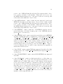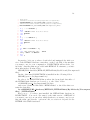
Download KSPECTRUM version 1.2.0 User Manual

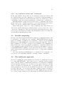
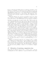
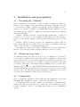
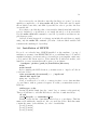
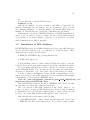
KSPECTRUM
version 1.2.0
User Manual
February 4, 2015
V. Eymet, Méso-star (www.meso-star.com)
LAboratoire PLasmas et Conversion de l’Energie, Université de Toulouse
Legal mentions
KSPECTRUM is a free software released under the terms of the CeCILL
license. This license is compatible with the GNU General Public License
(GPL). See the COPYING file within the main directory.
Méso-Star (www.meso-star.com) provides and distributes the sources of
the present code. By using this software, you agree to make a reference to
KSPECTRUM in any publication using results that have been obtained with
it. Support for the present code is no longer free. If you need to adapt the
code to your needs, for any computational request, or if you need to get
training in order to use the code, please contact Méso-Star ([email protected]) and we will provide an estimation of our fees.
Contents
1 Getting started
3
2 Description of the code
2.1 Production of high-resolution spectrum, full control of the uncertainty . . . . . . . . . . . . . . . . . . . . . . . . . . . . . .
2.2 Range of applications . . . . . . . . . . . . . . . . . . . . . . .
2.3 Physical hypothesis . . . . . . . . . . . . . . . . . . . . . . . .
3
1
3
7
8
2
2.4
2.5
2.6
2.7
2.8
2.9
2.3.1 Sub-lorentzian profiles and CIA . . . . . . . .
2.3.2 Broadening by the rest of the gas . . . . . . .
2.3.3 High-temperature transitions . . . . . . . . .
A better respect of spectroscopy . . . . . . . . . . . .
2.4.1 (no) line selection . . . . . . . . . . . . . . . .
2.4.2 (no) truncation of lines and “continuums” . .
Parallel computing . . . . . . . . . . . . . . . . . . .
The multi-pass approach . . . . . . . . . . . . . . . .
Estimation of remaining computation time . . . . . .
Not starting from scratch after a crash . . . . . . . .
Automatic tabulation of Lorentz and Voigt functions
3 Installation and prerequisites
3.1 Tweaking the “Makefile” . . .
3.2 Setting up array sizes . . . . .
3.3 Compilation . . . . . . . . . .
3.4 Installation of MPICH . . . .
3.5 Installation of LBL databases
.
.
.
.
.
.
.
.
.
.
.
.
.
.
.
.
.
.
.
.
.
.
.
.
.
.
.
.
.
.
4 Using the code
4.1 User input files . . . . . . . . . . . . . .
4.1.1 The “data.in” file . . . . . . . . .
4.1.2 The “options.in” file . . . . . . .
4.2 Other input files . . . . . . . . . . . . . .
4.2.1 Atmospheric composition . . . . .
4.2.2 Isotopologue abundances . . . . .
4.2.3 Narrowband intervals . . . . . . .
4.3 Running KSPECTRUM using MPICH or
.
.
.
.
.
.
.
.
.
.
.
.
.
.
.
.
.
.
.
.
.
.
.
.
.
.
.
.
.
.
.
.
.
.
.
. . . . . . .
. . . . . . .
. . . . . . .
. . . . . . .
. . . . . . .
. . . . . . .
. . . . . . .
OPENMPI
.
.
.
.
.
.
.
.
.
.
.
.
.
.
.
.
.
.
.
.
.
.
.
.
.
.
.
.
.
.
.
.
.
.
.
.
.
.
.
.
.
.
.
.
.
.
.
.
.
.
.
.
.
.
.
.
.
.
.
.
.
.
.
.
.
.
.
.
.
.
.
.
.
.
.
.
.
.
.
.
.
.
.
.
.
.
.
.
.
.
.
.
.
.
.
.
.
.
.
.
.
.
.
.
.
.
.
8
9
10
10
10
11
11
11
12
13
13
.
.
.
.
.
15
15
15
15
16
17
.
.
.
.
.
.
.
.
21
21
21
22
25
25
25
26
26
5 Results
27
5.1 Results files . . . . . . . . . . . . . . . . . . . . . . . . . . . . 27
5.2 More output files . . . . . . . . . . . . . . . . . . . . . . . . . 27
5.3 What’s next ? . . . . . . . . . . . . . . . . . . . . . . . . . . . 28
6 The fun stuff
29
6.1 Legal mentions . . . . . . . . . . . . . . . . . . . . . . . . . . 29
6.2 Questions and Answers . . . . . . . . . . . . . . . . . . . . . . 29
A Appendix - Validation
32
A.1 Low pressures / temperatures . . . . . . . . . . . . . . . . . . 32
A.2 High pressures / temperatures . . . . . . . . . . . . . . . . . . 32
3
1
Getting started
The first thing you should do is to declare your fortran compiler in the
F77 environment variable. In order to do so, you have to export the F77
environment variable in your .bashrc, .cshrc or .profile file; for instance, add
the following line into your .bashrc or .profile file:
export F77=”gfortran’’
in case you are not using the gfortran compiler, replace “gfortran” by
your local fortran compiler if needed (ifort, pgf, ...)
Then you need to type source .bashrc in order to take the modifications
into account. Replace “.bashrc” by whatever you are using. The purpose of
defining the F77 environment variable is to provide the correct compiler to
compilation commands that will be used later by the installation script. If
this variable is not defined, the name of your fortran compiler will be asked
every time a compilation will occur.
You need to use the “install kspectrum.bash” script that is provided with
the archive. This script should be placed in the same directory than the
provided zipped archive. Use the ./install kspectrum.bash command in
order to run it. This script will:
• Untar the archive, if the corresponding version of KSPECTRUM is not
already installed
• Make appropriate links in the newly created directory
• Go into the “data” directory, compile program “make data.exe” and
run in, in order to generate test files “composition.in”, “narrowbands.in”
and “molparam.in” (see section 4.2).
• Remind you to install LBL databases into the “data” directory (see
section 3.5).
Then you can go into the newly created directory (named “kspectrumX.X.X”
with “X.X.X” the version number) to continue the installation.
2
2.1
Description of the code
Production of high-resolution spectrum, full control of the uncertainty
KSPECTRUM has been designed to produce high-resolution spectrum of any
gas mixture, in any thermodynamical conditions, from line-by-line databases.
4
In practice, it is far from being the case: see sections 2.2 and 2.3, mostly because we have no idea of sub-lorentzian profiles and collision-induced absorption (CIA) in the general case. This code will be improved gradually when
our knowledge of spectroscopy evolves. Anyway, the purpose of the present
code is clearly NOT to produce spectrum that will be used in engineering
applications (i.e. spatial missions). Rather, it is intended at producing reliable spectrum that may be used for subsequent radiative transfer analysis
(production of radiative transfer parameterizations into planetary GCMs).
By “high-resolution” spectrum, we mean that the spectral resolution is
high enough so that individual lines are well resolved. This point is discussed below. The main purpose of producing high-resolution spectrum, is
the possibility to compute k-distribution data sets.
The main idea that lead to the development of KSPECTRUM is to produce a code that can compute high-resolution data for virtually any conditions, with a full control of the accuracy:
• Any value of ka (ν) has to be computed with a specified relative error
1 .
• The maximum relative error made when considering a linear profile
ka∗ (ν) between two computed values ka (νi ) and ka (νi+1 ) may also be
specified: 2 (see Fig. 1).
Ideally, when computing the absorption coefficient ka (ν) at a given wavenumber ν, the contribution of every line should be summed up:
ka (ν) =
N
X
ka,l (ν)
(1)
l=1
where ka,l (ν) is the contribution of the N lines index l to ka (ν). In
practice, it is impossible to use such a method to compute ka (ν) at high
spectral resolution, because the order of magnitude of N is typically several
hundreds of thousands, when not millions.
The first constraint of accuracy will be used to set up a faster algorithm:
we start by discretizing the infrared spectrum in a given number Nb of “narrowband” intervals, whose spectral limits are known. Let us take the example
of any spectral interval [νmin , νmax ]. Each one of the N lines will be examined for this interval. For a great number of lines, [νmin , νmax ] will be located
in the far wings, and therefore the values of ka (νmin ) and ka (νmax ) are not
|ka (νmax )−ka (νmin )|
is lower than the
very different. If the relative error = min(k
a (νmin ),ka (νmax ))
specified value 1 , then a constant value (for instance
ka (νmin )+ka (νmax )
)
2
can
5
Figure 1: Schematic representation of the computed ka (νi ) spectrum, and of
the maximal error made when considering a linear variation ka∗ (ν) between
two consecutive computed result points.
be taken as ka,l (ν), for every value ν ∈ [νmin , νmax ], with a total relative error
over ka (ν) that will be lower than 1 .
The second accuracy constraint (2 ) will be used for optimizing the spectral discretization: schematically, narrowband intervals [νmin , νmax ] will be
discretized in such a way that line centers are well described. Discretization
steps will take greater values in line wings. The computation of the spectral
grid uses a tabulation of the Lorentz and Voigt functions. The method is
explained below for a Lorentz line profile.
For an isolated Lorentz line, we have:
fL =
γL2
γL
+ (ν − νc )2
(2)
with γL the Lorentz line width, and νc = ν0 +δ.P the (corrected) wavenumber at line center.
This function can be written as:
fL =
1
1
γL 1 + x2
(3)
1
c
with x = ν−ν
. Next, function f (x) = 1+x
2 has been tabulated in order to
γL
determine a series of triplets [x1 , x2 , x3 ] such that for any value x0 ∈ [x1 , x2 ],
6
the maximum relative difference between f (x) and f ∗ (x) = f (x0 ) +
(defined for x ∈ [x0 , x3 ]) never exceeds 2 . Figure 2 may help.
f (x3 )−f (x0 )
(x
x3 −x0
− x0 )
Figure 2: Purpose of tabulating function f (x): for any x0 ∈ [x1 , x2 ], the
maximum relative difference between f and f ∗ is lower than the imposed
value 2 .
In practice, for the computation of the spectral grid: starting from a
wavenumber value νi , the algorithm will have to determine the next grid
point νi+1 (see Fig. 1). For every line l whose center wavenumber is within
[νmin , νmax ], the code will have to identify the triplet [x1,l , x2,l , x3,l ] so that
ν −ν
xi,l = iγL,lc,l ∈ [x1,l , x2,l ]. We know that the position of the next grid point
could safely be taken at x3,l , if line l was alone. Taking the minimum value
νi+1 = min(νi+1,l = γL,l x3,l + νc,l ) (over all lines present in the interval)
ensures that the relative difference between ka and ka∗ never exceeds 2 over
[νi , νi+1 ].
q
1 y
The principle is exactly the same for the Voigt function fV (ν) = ln(2)
π γD π
p
p
c
with x = ln(2) ν−ν
, y = ln(2) γγDL , and γD the Doppler linewidth. This
γD
function depends on y, the ratio of Lorentz and Doppler linewidths. This
function will therefore have to be tabulated as a function of x, but also as a
function of y.
I really don’t see the point in giving any more details. If anyone ever reach
this point without falling asleep and reads this, please send me an email at:
[email protected]
A special mention should be made tough to the issue encountered for
2
R +∞
e−t
−∞
y 2 +(x−t)2
dt,
7
meshing the spectral grid between close strong lines. In the case νi is located
between two strong lines, the value of νi+1 computed by the above-described
algorithm may be too far from νi to satisfy accuracy criterion over 2 , because
of the strong overlap between the two lines. In this case, a special treatment
should be applied for a correct discretization of wavenumbers.
2.2
Range of applications
KSPECTRUM is currently using the following LBL databases: HITRAN
(2004 and 2008) [1, 2], HITEMP (2004) [3] (H2 O, CO2 , CO and OH only),
HITEMP (2010) [4] (H2 O, CO2 , CO, N O and OH only) and CDSD [5] (CO2
only). The code uses the HITRAN database for temperatures lower than a
user-defined temperature “T hitemp” (defined in the “data.in” file, see section /refpara:userfiles). For temperatures greater than this value, it lets the
user chose between HITEMP or CDSD for CO2 lines, and will automatically
use HITEMP for H2 O, CO and OH transitions. The temperature upper
limit of validity of the present code is therefore the same as the HITEMP
database (about 1000K), except when computing the spectrum of a pure CO2
atmosphere: the CDSD database is supposed to be accurate up to 3000K.
No physical limit is imposed for pressures. However, the upper limit
in terms of pressure is probably what is found at ground level on Venus:
ground pressure is 92 bars, and ground temperature is 735K. At such levels
of pressure and temperature, the atmosphere is in super-critical thermodynamic state, and can no longer be considered as a mixture of gas. Therefore KSPECTRUM should probably not be used for a pressure greater than
100atm. The lower pressure limit will be imposed by the code itself, and more
specifically by the spectral discretization algorithm. It may crash for values
of the pressure lower than 10−7 atm, because spectral lines are so narrow
that wavenumber steps are really small (≈ 10−7 cm−1 ). Besides the fact that
the computation of the spectral grid may take a lifetime in these conditions,
such small wavenumber steps may not be properly taken into account by the
algorithm.
In terms of molecules, the HITRAN database takes into account the transitions of 42 (for the 2008 version) molecular species, along with their isotopes. The list of molecules can be found in the HITRAN documentation
[1], or directly in the “data/molparam.txt” file.
Other limits may be imposed for specific gas mixtures. See section 2.3
for more details.
8
2.3
Physical hypothesis
This section presents how we manage the fact that there is a lack of available
spectroscopic data for various aspects of the theory.
2.3.1
Sub-lorentzian profiles and CIA
The main issue is that we have very little knowledge about:
• The real line shape, for each molecule, at each wavenumber. We know
that CO2 lines have a sub-lorentzian behavior in line wings, which is
why thermal infrared signals can be transmitted from ground level up to
space in very specific near-IR spectral windows through the otherwise
very thick atmosphere of Venus.
• Collision-induced absorption (CIA), that are mainly due to the fact
that in high pressure and/or high temperature conditions, collisions
between molecules temporarily create new molecular species, with their
own energetic transitions.
Sub-lorentzian profiles have been studied since 1969: in [6], the Lorentz
profile fL (ν − ν0 ) is corrected by a function χ(ν − ν0 ) that accounts for the
sub-lorentzian nature of the lineshape. Function χ(ν − ν0 ) is given for pure
CO2 and for mixtures of CO2 and other species (N2 , He, Ar, O2 , H2 ) in very
specific spectral ranges, for various values of the temperature. In [7] and [8],
function χ is given respectively for pure CO2 and for CO2 broadened by O2
and N2 , in the 4.3 µm region, for different temperatures. It was then shown
in [9] that function χ is asymmetric (with respect to ν0 ) for CO2 in the 4.3µm
region, at 296K.
Finally, Perrin and Hartmann [10] and Tonkov et al. [11] provide χ functions for pure CO2 , respectively in the 4.3 µm region, for T ∈ [190 − 800]K
and in the 2.3µm region, at 296K. These results are used in KSPECTRUM in
order to compute χ profiles. Various options (see section 4) let the user chose
whether χ functions from the literature must be used in their strict range
of validity, or if they have to be used in different spectral ranges / for other
molecules than CO2 .
Collision-induced transitions are even more difficult to take into account:
there are some measurements from Tonkov at al. [11] in the 2.3 µm region,
at room temperature. Central wavenumbers and intensities are given for 8
transitions, but the authors clearly state that the data they provide should be
considered with caution, because of the large uncertainties of their measurements/computations. Other measurements of CO2 CIA have been reported
9
in the literature: [12, 13, 14, 15]. Data (lines central wavenumber and intensity) are either not provided, or given with poor accuracies, or provided in a
very limited range of validity (in very specific spectral regions, for only one
value of pressure and temperature, etc). Practically, it is not possible to use
literature results to take into account collision-induced (or pressure-induced)
absorption lines properly.
The only results that could practically be used for computing CO2 CIA
is the work from Gruszka and Borysow [16]. In addition to the paper, the
authors provide a fortran computer code [17] that will compute CIA for
CO2 , in the 0-250cm−1 wavenumber range, in the 200-800K temperature
range (this was motivated by studies of Venus’ atmosphere, since CIA is a
dominant source of opacity in the far-infrared (between 0 and 550cm−1 ) on
Venus’ atmosphere [18] where temperature reach 735K at ground level). This
code has been modified (for computing CIA coefficient for only one value of
ν) and integrated into KSPECTRUM 1 . CIA of CO2 will therefore accurately
be taken into account within these validity ranges. Options (see section 4)
allow the use of CIA computation outside these validity ranges. In particular,
the 2.3 and 4.7µm spectral bands of CO2 are not taken into consideration.
2.3.2
Broadening by the rest of the gas
Another limitation of the code is the hypothesis that is done concerning γother :
lines of a given species i can be broadened by collisions with the same species
i, or by collisions with other species j. The self-broadened half-width γself
given by LBL databases, and that account for collisions between molecules
of the same species, can be considered as reliable. However, LBL databases
also give us parameter γair , the air-broadened half-width, that corresponds
to the broadening of lines by collisions between species i and... the air on
the terrestrial atmosphere !
Of course, when computing a spectrum for a non-terrestrial atmosphere,
parameter γother should not take the value of γair indicated in LBL databases,
because the rest of the gas is no longer Earth’ air. However, we have no other
choice than taking γother = γair , because there are no other data available.
This choice can be justified by the fact that γother will probably never be very
different from γair anyway.
1
Note that M. Gruszka’s code is not supposed to be redistributed. However, the authors
mention that the code can be used in academic applications, such as KSPECTRUM .
10
2.3.3
High-temperature transitions
We know that (a large number of) new transitions are activated at high
temperatures. The CDSD database offers a solution for CO2 lines: it is
valid up to 3000K [5]. A new HITEMP database is in preparation, that
should cover a huge number of high-temperature transitions for H2 O. More
generally, the accuracy and range of application of public LBL databases is
clearly increasing. However, the accuracy of spectra computations always
depend on the available LBL parameters. The current level of knowledge
will always impose a limitation on the accuracy of numerical simulations.
WARNING: there are some inconsistencies within the current HITEMP
database: some values of the γself parameter are null ! This is an issue
because, in the case you want to produce a high-resolution spectra for a
single molecular species, only this parameter will be taken into account in
the computation of the Lorentz line width γL . A null γself will result in a
null value for γL , and this will end in a crash of the code during spectral
discretization. The spectral discretization algorithm has been improved in
order to detect null values of γself ; in this case, instead of using a null value,
the γself parameter will be set to the closest non-null value found among the
LBL database.
2.4
A better respect of spectroscopy
The general idea of KSPECTRUM is to ensure the simple accuracy criterion
that are discussed in section 2.1. In order to achieve this for any situation (gas
mixture composition, values of temperature and pressure), it is absolutely
necessary that the coding is well separated from the physical problem. In
particular, the available computing power should not impose limitations on
the versatility of the code. We believe this is possible with to-days masscomputing power.
2.4.1
(no) line selection
Existing computation codes that can produce high-resolution spectrum always involve line selection at some point. The purpose of selecting lines is to
reduce the total computation time, by reducing the number of lines N whose
contribution has to be computed at each wavenumber point ν (see Eq. 1).
However, KSPECTRUM does not need to select lines that have to be
taken into account: the contribution of all transitions are effectively computed. See section 2.1 for details (accuracy parameter 1 ).
11
2.4.2
(no) truncation of lines and “continuums”
In the same manner, line profiles are not truncated as they probably would
in a classical approach: the contribution of each line at each wavenumber ν
is computed, no matter how far from the line center ν is. This is also a direct
consequence of the way accuracy parameter 1 is taken into consideration.
KSPECTRUM does therefore not need to use a “continuum” that is classically added to the computed spectrum to correct line truncation side-effects.
Values of ka (ν) are computed with a specified relative accuracy 1 .
2008/12/09 update: this is no longer completely true, since I have enabled a line profile truncation possibility in the code (see section 4.1, end of
“options.in” description). This option should be used with great care, since
it is most probable that very intense and distant lines will not be taken into
account when truncating line profiles.
2.5
Parallel computing
Because of accuracy requirements that are imposed, computation times could
be prohibitive on a single-processor machine. KSPECTRUM has been designed for running on multi-processor machines / clusters. It uses MPICH
instructions so that multiple processes can be run at the same time. The four
time-consuming loops of the code have been parallelized. As communication
times between processes are negligible (compared to computation times), the
total computation time will effectively be divided by the number of processors KSPECTRUM is running on (provided that all processors / machines
in the cluster run at the same speed and are free of other time-consuming
processes.)
Of course, this means MPICH has to be installed before using the code.
See section 3.4 for installing MPICH / creating a cluster of machines.
2.6
The multi-pass approach
We are now talking about the limitations of fortran 77, which has been used
for coding KSPECTRUM . The source code is constantly checked against
array overflows, unused or uninitialized variables, etc (classical programming
errors), and there should be no problem of bad coding. However, one limitation of fortran 77 is that the size of each array has to be declared. And
in the present case, the most obvious limitation is the size of the arrays that
hold the LBL data. For a typical atmosphere (Earth, Venus), less than 10
molecular species have to be taken into account, which gives a total number of lines of approximately 2.105 when using the HITRAN LBL database.
12
However, when using the CDSD database for CO2 lines, the number of lines
that have to be taken into account can exceed 107 . And there is no way 9 arrays of size 107 can be declared on a classical machine that holds 1GB RAM
(KSPECTRUM actually needs to read 9 LBL parameters from databases,
which imposes the declaration of 9 data arrays). The default size of theses arrays is 2.106 , and can be reduced for low-memory configurations (see
section 3.2).
With such a limitation, the only way several millions of lines can be taken
into account is to perform a multi-pass computation: for instance, when the
user specifies the use of the CDSD database for CO2 transitions, 10 millions
lines have to be taken into account (for CO2 only). With an array size
of 106 , KSPECTRUM will read the first 106 lines (first pass), and perform
the computation of the ka (ν) spectrum with these first set of lines (it will
actually compute the contribution of this first million of lines to the final
result). Then it will perform a second pass, using the second million of lines
in the database: it will compute the contribution of the second million of lines
to the final result. And so on, until all lines have been taken into account.
An attentive reader could tell me this approach is incorrect if applied to
the spectral discretization. Indeed, in order to compute a correct spectral grid
for any [νmin , νmax ] narrowband spectral interval, the algorithm needs to take
into account ALL the lines whose central wavenumber is within [νmin , νmax ].
When reading chunks of LBL database, it is obvious that line parameters are
missing for many [νmin , νmax ] intervals. This is the reason why the spectral
discretization algorithm does not use the multi-pass approach: it automatically looks into every LBL database file to identify relevant line parameters
for each [νmin , νmax ] interval (in practice, a complete parsing of LBL data files
is necessary in order to accelerate the process of line identification). This is
also why LBL data files must be readable by any KSPECTRUM process (see
section 3.5).
Finally, we should mention that the total computation time for a multipass computation is not higher than for a 1-pass computation, since all lines
have to be taken into account anyway. The spectral discretization is performed during the first pass and is known for subsequent passes, which does
not increase the total computation time. The main advantage of this multipass approach is the possibility to run the code on low-memory configurations.
2.7
Estimation of remaining computation time
When using the multi-pass approach, the code will be able to guess the
remaining time before the computation of a spectra is finished for the current
13
atmospheric level. This is only possible for a multi-pass computation, because
in order to have an estimation of the remaining computation time, the code
needs to know the spectral grid (that is computed during the first pass of
each atmospheric level), and how many points of the grid have already been
computed. The “status.txt” file will report the estimated time (in real-life
date/hour format) when the computation for the next atmospheric level is
going to start.
2.8
Not starting from scratch after a crash
Imagine you want to compute the spectrum of a given atmosphere mainly
composed of CO2 , using the CDSD database, over 80 atmospheric levels,
for the whole infrared range. This should typically require several weeks
of CPU time, even for a multi-processor machine or a small-size cluster. If
you run KSPECTRUM on a dedicated multi-processor machine, if no one
else has access to this machine, and if there is no power cut during all the
computation, there should be no problem. Now imagine you run it on a PC
cluster, with many other users that daily access these machines. Someone will
eventually reboot one of these machines, crashing your whole computation. I
would say that you can not decently expect more than 48 hours between two
consecutive reboots. In these conditions, the computation will never end.
Fortunately, KSPECTRUM can resume a computation if a crash has
been detected. It will start over from the last backup point, which occurs
every time the computation of the spectrum has been achieved on a given
narrowband interval. Multi-pass computations will be resumed as well.
2.9
Automatic tabulation of Lorentz and Voigt functions
Section 2.1 presents the principle of the spectral discretization algorithm used
in KSPECTRUM . It needs a tabulation of the Lorentz and Voigt functions.
These tabulations depend on the value of 2 , the user-defined accurately
that is required over the spectral grid. Tabulation files reside within the
“data” directory, and are indexed according to the value of 2 : for instance,
“data/tabulation lorentz0.01.txt” is the file where [x1 , x2 , x3 ] triplets have
been recorded for the Lorentz function, and for an accuracy 2 =0.01 (a 1%
uncertainty).
Values of 1 and 2 may be changed by the user (see section 4.1). If the
user specifies a value of 2 for which there is no known file, KSPECTRUM will
have to perform the tabulation prior to start the spectrum computation. Of
14
course, the code will record tabulation results in the appropriate file, so that
the tabulation for this value of 2 will never have to be performed again. This
tabulation is performed by a fully parallel loop, so that it can benefit from
the number of processors KSPECTRUM has been launched on.
15
3
3.1
Installation and prerequisites
Tweaking the “Makefile”
Before compiling, you will have to find out what compilation options are
right for your compiler, and your machine. Open the “Makefile” file, and
look at variables “FOR”, “ARCH” and “OPTI”. Variable “FOR” is used to
specify your fortran 77 compiler. As KSPECTRUM uses MPICH, you will
most likely use the “mpif77” compilation command, that has been installed
along with MPICH.
Variable “ARCH” is used to specify machine architecture. “-m486” is
probably a good choice for a PC running a 32bits linux. Use the documentation of your fortran compiler to find out what architecture option you can
use.
Variable “OPTI” is used to specify code optimization options. The default options should be enough. Please note that you definitely must use
option “-Wno-globals” for compiling parallel code.
You might also want to set variable “DEBUG” (look for its definition in
the file). You can expect faster execution times if you leave it empty.
3.2
Setting up array sizes
As explained in the previous section (see 2.6), one limitation of fortran 77
code is that you must define array sizes before compilation. Arrays sizes
used by the present code are defined within the “includes/max.inc” file. You
should at least look at it before compiling, and more precisely at the value
of variable “Nline mx”. Its default value is 2000000 (2.106 ), because most
machines will be able to compile KSPECTRUM with this value (you need
at least 1GB RAM). You can enable a lower value if you do not have enough
memory. The code will then perform a multi-pass computation (see section
2.6), but total computation time will not be increased.
3.3
Compilation
Once you checked compilation options and array size definitions, you can use
the make all command in order to compile the executable file.
If compilation fails, use the compiler error message to determine what
went wrong. The most probable error causes are: a bad definition of architecture compilation option, or an inappropriate value in code optimization
options.
16
If you ever need to modify the source files (in directory “source”), you can
quickly recompile the code using make all again. This will only recompile
the modified source files, and link objects files in order to produce the new
executable file.
If you have to modify the value of any variable defined in includes files (directory “includes”), you will have to recompile the whole code from scratch.
Use the make clean all command to erase all objects files, and then recompile them properly.
Odd errors may happen if you change an include file and then recompile
using only the make all command (old value of the modified variable will
remain in the unchanged object files).
3.4
Installation of MPICH
If you do not already have MPICH installed on the machine / group of
machines you want to run KSPECTRUM on, you will first have to download
mpich2 from http://www.mcs.anl.gov/research/projects/mpich2 ; make sure
you download the latest version. Next, untar the downloaded archive, and
install it on every system that will be part of your cluster:
./configure –prefix=/path/to/installation/directory
make
make install
Before running the MPD daemon, you must create a “.mpd.conf” file in
your home folder:
echo secretword=[secretword] >> /.mpd.conf
chmod 600 .mpd.conf
using any “secretword”.
Next, you will need to be able to connect via ssh to every other machine
of your cluster, with no password request. For this, you must first create a
DSA key:
ssh-keygen -t dsa
leaving all fields blank (use the “enter” key to answer each question).
Then you will have to add this DSA key to the list of authorized keys:
cd .ssh
cat id dsa.pub >> authorized keys
Finally, create the list of machines that belong to your cluster. This list
must reside within the “mpd.host” file on your home folder. Each line must
contain the name of the machine, by order of availability:
[host1].[domain]
[host2].[domain]
[host3].[domain]
17
etc
You can then try to run the MPD daemon:
mpdboot -n [#]
with [#] the number of hosts you want to run MPD on (typically, the
number of machines in your cluster). If you encounter no error, you can
use command “mpdtrace” to check the number of hosts the MPD daemon is
running on. This should give you the list of machines in your cluster.
Alternatively, you can use OPENMPI instead of MPICH. Installation is
easier, you do not have to create a “.mpd.conf” file, and the MPD daemon
does not have to be started (mpdboot) prior to code execution. Programmation instructions are fully compatible.
3.5
Installation of LBL databases
KSPECTRUM needs to access LBL databases in order to run. LBL databases
are not provided with the code, you will have to download them. These
databases can be found on FTP servers:
• HITRAN & HITEMP: ftp://cfa-ftp.harvard.edu
• CDSD: ftp://ftp.iao.ru
You should first connect to either of these FTP sites in order to locate the
top-level directory for the required database (probably somewhere in /pub )
If you are using MacOS, it is possible to use the ”Go/Connect to server”
option within the Finder. Use ”anonymous” as login, and your e-mail address
as password. Then just ”copy” and ”paste” the top-level directory adress.
It is also possible to use wget if you can only use command-line tools (for
instance, if you try to access ftp sites from a remote machine); the example
command line below is given for HITEMP-2010:
wget -drc –user=anonymous –password=[your email address] ftp://cfaftp.harvard.edu/pub/HITEMP-2010 .
This will litteraly download the whole “HITEMP-2010” directory right
into the directory where this command was issued.
The code expects to find LBL databases in the “data” directory. Of
course, you have to download LBL databases in a directory that is common
to all machines the code will run on (shared disk), so that each process will
be able to access the LBL databases through the “data” directory.
LBL data file directories must be the following:
• “data/HITRAN2004”: must contain the uncompressed by-molecule
HITRAN data files in its 2004 version. If you create a link, it must
18
point to the “HITRAN2004/By-Molecule/Uncompressed-files” directory on the local disk of each machine. When the code is set to use
the HITRAN2004 database (see “options.in” in the 4.1.2 section), this
folder must exist within the “data” folder.
• “data/HITRAN2008”: must contain the uncompressed by-molecule
HITRAN data files in its 2008 version. If you create a link, it must
point to the “HITRAN2008/By-Molecule/Uncompressed-files” directory on the local disk of each machine. When the code is set to use
the HITRAN2008 database (see “options.in” in the 4.1.2 section), this
folder must exist within the “data” folder.
• “data/HITEMP”: must contain the old HITEMP database uncompressed data files. If a link, it must point to the “HITEMP/uncompressed data” local directory.
• “data/HITEMP-2010”: must contain the new (2010 version) HITEMP
database. Within this folder, you must have 5 folders named “CO2 line list”,
“CO line list”, “H2O line list”, “NO line list” and “OK line list”. Within
each one of these directories, you must create two other directories: one
named “Compressed files” that contains original compressed data files
(*.zip files) and a second one named “Uncompressed files” that contains un-zipped files (*.par files) for the molecular species. Upper /
lower case matters, the code will look into this directory structure as
mentionned in this section.
• “data/CDSD”: must contain CDSD uncompressed data files. If a link,
it must point to the “CDSD 1000 UPDATED/uncompressed data” local directory.
• “data/CDSD-HITEMP”: must contain CDSD-HITEMP uncompressed
data files.
• “data/CDSD 4000”: make it a link (preferably) to a folder that contains every single one of the 2768 uncompressed LBL files for the
4000K version of CDSD. This version of the database holds information for more than 628 millions of transitions, and the total weight of
the database is 73 Gb once uncompressed (23 Gb for the compressed
files that can be downloaded from the FTP site). The files in this
folder should not be renamed: their names are “cdsd 00220 00230”,
“cdsd 00230 00240”, “cdsd 00240 00250”, etc. You will have to find
a way to unzip every zipped file that has been downloaded, using for
instance a base script like this one:
19
1
2
3
4
5
#!/bin/bash
# TARGET is the folder containing target files (i.e. zipped files)
TARGET=$HOME/ l a b _ d a t a / CDSD_4000 / c o m p r e s s e d _ f i l e s
# RESULT is the folder containing resulting files (i.e. unzipped files)
RESULT=$HOME/ l a b _ d a t a / CDSD_4000 / u n c o m p r e s s e d _ f i l e s
6
7
8
9
10
11
12
13
14
15
16
17
18
if [
then
echo
echo
exit
fi
if [
then
echo
echo
exit
fi
! −d "$TARGET" ]
’TARGET f o l d e r d o e s n o t e x i s t : ’
$TARGET
1
! −d "$RESULT" ]
’RESULT f o l d e r d o e s n o t e x i s t : ’
$RESULT
1
19
20
21
22
23
24
25
f o r FILE i n $TARGET / ∗ . z i p
do
echo ’Now u n z i p p i n g f i l e : ’ $FILE
u n z i p " $FILE " −d $RESULT
done
exit 0
In practice, let’s say you have downloaded and unzipped the 2008 version of the HITRAN database somewhere on the local disk of the machine
you want to use for your computation. KSPECTRUM will need the “bymolecule” data files that are provided with HITRAN. For instance, you have
these files in the following folder:
$HOME/LBL databases/HITRAN/HITRAN2008/By-Molecule/Uncompressedfiles/
On the other hand, KSPECTRUM is installed in the following folder:
$HOME/great codes/kspectrum1.2.0/
In order to let KSPECTRUM know where the by-molecule data files of
the HITRAN2008 database are located, go to the “data” folder:
cd $HOME/great codes/kspectrum1.2.0/data
and create a symbolic link called “HITRAN2008” to the folder that contains the data files:
ln -s $HOME/LBL databases/HITRAN/HITRAN2008/By-Molecule/Uncompress
files/ ./HITRAN2008
Here you go. You have just installed the HITRAN2008 database in
KSPECTRUM . You can do the same for the 2004 version of HITRAN if
you want to use it (you can select which database you want to use by setting the right option in the “options.in” file, see section 4.1.2) and for the
HITEMP and CDSD databases.
20
Frequent updates are published about HITRAN data. If you want to use
these new data files, follow these directions: let’s say you want to download
the update for SO2 from the HITRAN website (section “HITRAN updates”).
Download the updated file “09 hit09.par” within the folder that contains
your by-molecule data files. KSPECTRUM will still look for files that are
labelled “08”, so you will have to link the new file to the old one: within the
by-molecule data folder, rename the old SO2 file:
mv 09 hit08.par 09 hit08.par.ori
Then create a link from the new file to the old one:
ln -s 09 hit09.par 09 hit08.par
Repeat this step for every update file.
Finally, there is also supplemental data, that is not directly provided
among the “by-molecule” data. These files reside within the “HITRAN2008/Supplemental”
folder. There are currently three data files within this “supplemental” folder:
“30 hit08.par”, “35 hit08.par” and “42 hit08.par”. In order to add then to
your “by-molecule” folder, you can just copy/paste them, or once again create
symbolic links (does not take more disk space); within your “by-molecule”
data folder, type the following commands:
ln -s ../../Supplemental/30 hit08.par .
ln -s ../../Supplemental/35 hit08.par .
ln -s ../../Supplemental/42 hit08.par .
21
4
Using the code
4.1
User input files
There are two files in the main KSPECTRUM folder: “data.in” and “options.in”. The “options.in” file is where the user can chose between several
options, for each algorithm. The “data.in” file is where the user can specify
the numerical values of a number of variables the code will use. Below is a
description of these two files.
4.1.1
The “data.in” file
• Section “Production of k spectrum”: the user must specify the values
of 1 and 2 (see section 2.1). Default values are 1%.
• Section “Narrowband discretization”: the user can specify the minimum and maximum values of the wavenumber range the spectrum will
be computed for, and the maximum error percentage over the Planck
intensity for discretization of the wavenumber range into narrowband
intervals. These data should be specified only if the user chose to compute the narrowband discretization instead of using pre-defined narrowband intervals (via an option in the “options.in” file). Refer to the
description of the corresponding option for more details. Finally, the
user should specify the value of the constant spectral step to use (when
required in “options.in”).
• “Parallel computing”: the user should specify the number of chunks
the code will use for the computation of the k spectrum. Once the
spectral grid is computed, the code knows the number of k values that
will have to be computed. The computational load that will be sent to
each process is the number of k values divided by the number of chunks.
If this number of chunks is large, each process will have to compute a
small number of k values. A chunk will be sent each time a process is
found idle. The advantage is that if processors run at different speeds
/ have to run other processes, processes that run on slow processors
will be sent a lower computational load (fewer chunks), and processes
that run of fast processors will be sent a greater number of chunks.
• Section “Levels and narrowbands limits”: first, the high-temperature
level has to be indicated; this value is used to switch between HITRAN
(at low temperatures) and HITEMP or CDSD (at high temperatures).
By using a high value (higher than the highest value of temperature
22
you want to compute spectrum for) you can be sure only HITRAN
is used. The user can then specify the indexes of the first and last
atmospheric level / narrowband interval if only a limited number of
atmospheric levels / narrowband intervals should be treated instead of
every atmospheric level / narrowband interval. The choice itself is done
via the corresponding option.
• Section “Special options for degraded mode”: the user should provide here values the code will use when running into degraded mode.
Three values are used for the degraded spectral discretization algorithm
(number of line widths to consider in the definition of a line’s central
zone, the number of points used to discretize lines central zones and
the number of points used to discretize regions between lines). The
next parameter is the minimal distance (from current value of ν) to
the central wavenumber of each transition that is used for line profiles
truncation. Then the user should provide the percentage of transitions
(in terms of reference line intensities) that will be neglected by the
reference spectral discretization algorithm.
One last value is the value of c used by the “convergent-k” algorithm (see “options.in”): when this algorithm is enabled, transitions
are sorted according to their intensities, and the contribution of most
intense lines are added first when computing k(ν). The algorithm
will regularly update and check the evolution of k(ν): this history
with ki (ν) the succesis expressed as successive values of αi = kkni (ν)
(ν)
sive values of k(ν) that have been recorded, and kn (ν) the current
value of k(ν) (the last recorded
value). Convergence is reached once
αn − αn−1 < max αi − αi−1 ∗ 1 ∗ c with 1 the maximum error percentage allowed over k(ν) and c a value that provides the user a mean
to control this convergence criterion.
4.1.2
The “options.in” file
• Section “Narrowband discretization”: the user can chose between computing automatically the narrowband discretization or use pre-defined
narrowband intervals. If the narrowband discretization has to be performed by the code, it will use the three corresponding values in the
“data.in” file (section “Narrowband discretization”): the specified wavenumber range will then be discretized into a number of narrowband intervals, and the Planck intensity relative variation between the limits of
each narrowband interval will not exceed the specified maximum er-
23
ror percentage over Plank intensity. If the user decides to use a predefined narrowband discretization, a file called “narrowbands.in” must
be found in the “data” directory. This file should contain the number
of narrowband intervals, and the wavenumber limits of each interval.
See the provided “data/narrowbands.in” example file.
• Section “Choice of spectroscopic database”: A first option makes possible to use custom LBL databases (parts from existing databases for
instance). The corresponding LBL files have to be written using the HITRAN format. These files must reside within the “data/custom LBL”
folder, and must be named according to the molecular species the transitions they contain belong to, for instance “custom H2O.txt” or “custom CO2.txt”.
When custom LBL databases are not used, the user has to decide
whether the default HITRAN database to use is the 2004 or the 2008
version; the corresponding link must be established within the “data”
folder (see section 3.5). The user can then choose between the CDSD1000, the CDSD-1000-updated, the CDSD-HITEMP or the CDSD-4000
databases for CO2 and between HITEMP (old version) or HITEMP2010 for H2 O, for a temperature greater than “T hitemp” (whose value
was set in the “data.in” file).
• Section “Composition”: the user should specify whether the code will
use only the main isotope or all isotopes when the concentration of
isotopes are not specified for a given molecule.
• Section “Line profiles”: first, the user can select to use either the
Lorentz or the Voigt line profile; the user has then to chose whether or
not the sub-lorentzian nature of lines has to be taken into consideration.
See section 2.3 for more information about how the code will manage
sub-lorentzian profiles. In particular, function χ is given for pure CO2
only, in specific spectral ranges, and for a limited range of temperature.
The user can chose to use literature data outside its range of validity
(over the whole IR spectrum), and for other molecules than CO2 (use
with great care !). Finally, the asymmetric nature of function χ can be
taken into account, but results will not be very different from using a
symmetric function.
• Section “Collision-Induced absorption”: the use can chose whether or
not collision-induced absorption (CIA) should be simulated for CO2 .
See section 2.3. The user can subsequently choose CIA computation
from the work of Gruszka [16] or Baranov [19] or both, in which case
24
both sources of opacity are added. The user can also chose to compute
CIA coefficients outside the wavenumber validity range (0-250 cm−1 )
and the temperature validity range (200-800 K).
• Section “Code behavior”: the user can chose to display or not computation times on screen. Finally, it should be specified whether the
code has to resume an interrupted computation, or start again from
the beginning.
• Section “Sensitivities”: the user can chose to compute sensitivities of
results (cross-section and absorption coefficient) to total pressure, temperature and species concentrations. When computation of sensitivities
are enabled, results are recorded in files “results/dk dXXX”.
• Section “Levels and narrowbands limits”: the user must chose whether
the code has to compute a spectrum for every atmospheric level / narrowband interval, or only for a limited number of levels / intervals. If a
limitation is imposed, the code will use the corresponding values found
in the “data.in” file (section “Levels and narrowbands limits”).
• Section “Spectral discretization algorithm”: the user should choose between the reference spectral discretization algorithm, a degraded spectral resolution, using a constant spectral step or using a spectral discretization based on line centers . Degraded resolution will compute
the spectral grid faster than the reference algorithm, and will also make
the computation of the spectrum faster since less points will have to
be computed. However, the accuracy criterion 2 will not be satisfied
by any other algorithm than the reference scheme. This degraded resolution algorithm takes input values (see “data.in”). When using the
reference spectral discretization algorithm, the user should also provide the accuracy level that will use the special spectral grid algorithm
for wavenumbers located between close strong lines. A value of 0 disables this special algorithm: wavenumbers νi will be computed using
the standard meshing algorithm based on Lorentz and Voigt functions
tabulation, described in 2, but remember that in this case, the spectral
grid may be too coarse between strong lines. A value between 1 and 4
will enable the special meshing algorithm. The highest the value, the
more accurate this algorithm will be (there will be more values of νi ,
therefore making the k-spectra computation longer). A value of 3 may
be enough in most cases.
• Section “line truncation and selection”: the user has the ability to truncate line profiles at a fixed distance from line centers or for a multiple of
25
the line width (see “data.in”). When this option is used, the accuracy
criterion 1 is no longer satisfied. Line truncation will make kspectrum
computations much faster. When a truncation is required, the user has
also the ability to set the contribution of constant lines to zero, so that
absorption is null between very distant lines.
A last option enables weak lines rejection: in order to speed up calculations, the computation can be performed using only the stronger
lines (those who have the highest intensities). This option enables
the“convergent-k” algorithm that sorts lines according to their line
intensity (computed at the current mixture’s temperature) and adds
the contribution of intense lines first until the convergence criterion is
reached. This criterion can be adjusted using the corresponding value
in the “data.in” file.
4.2
4.2.1
Other input files
Atmospheric composition
is provided via the “data/composition.in”. This file must contain a label
for the atmospheric composition (could be used in future version for planetspecific physics, such as sub-lorentzian profiles or CIA), the number of atmospheric levels, the number of molecular species, the label of each molecular
species, and, for each atmospheric level: altitude in km (unused at present
date), pressure in atm, temperature in Kelvin, and the molar fraction (or
partial pressure) of each molecular species. See the example file.
Molecule labels have to be identical to labels used in the HITRAN nomenclature. Labels of molecules defined in the HITRAN database can be found
in the “data/molparam.txt” file. They are obvious for most species: “H2O”
is used for water vapor, “CO2” for carbon dioxide, etc. Please use capital letters when providing molecule labels in the “data/composition.in” file,
and note that molecule labels must be provided between brackets (example:
“[H2 O]”) so that the code can identify molecular species.
4.2.2
Isotopologue abundances
For each molecular species that is provided in the “data/composition.in” file
(i.e. molecules whose label is unknown from the HITRAN nomenclature),
information has to be provided about these molecules in the “data/molparam.in” file. In particular, the abundance of each known isotopologue
should be provided, for each (P/T) level. See the provided example file produced by the program that can be found in the “data/make composition.for”
26
source file.
One remark about isotopologues: when no isotopic abundance has been
explicitly provided via the “data/molparam.in” file for a given molecular
species, the algorithm can chose to take into account only the main isotope
of this species, or use all isotopes whose line parameters are provided in LBL
databases. The user can chose between both behaviors in the “options.in”
file (see section 4.1.2).
4.2.3
Narrowband intervals
have to be provided in the “data/narrowbands.in” file, provided that the user
chose to use a pre-defined narrowband discretization (see section 4.1). This
file must contain the number of narrowband intervals, and, for each interval,
its lower and upper limits, in terms of wavenumber (in cm−1 ).
4.3
Running KSPECTRUM using MPICH or OPENMPI
Once everything is installed and the executable file “kspectrum.exe” file has
been compiled, you can try to run a computation. I would recommend that,
for the first time, you run KSPECTRUM over a single atmospheric level, for
a single narrowband interval, using a simple atmospheric composition (the
provided example composition for instance).
Use the following command to run the code:
mpirun -np [#] kspectrum.exe
with [#] the number of processes that have to run.
Because communication times are small compared to computation times
in KSPECTRUM , it is a good idea to chose a number of processes equal to
the number of (physical) processors of your cluster, plus one. One process, the
master process, is dispatching computational loads to every other processes
(slave processes), and gathering results from them. It does not require any
significant CPU time, therefore it is OK to have a number of slave processes
equal to the number of processors, so that each slave process can use a
processor (or each processor will have only one slave process running on it).
In practice, if your cluster is composed of n processors, you can use:
mpirun -np n+1 kspectrum.exe
27
5
Results
5.1
Results files
KSPECTRUM will produce results files in the “results” directory. There
is one file per atmospheric level. Files are named “k***” with “***” the
index of the atmospheric level. For instance, “results/k001” is the result file
produced for the first atmospheric level (with the highest pressure level).
Each file contains 3 columns. The fist column gives values of wavenumbers, in cm−1 . The second column is the total cross-section of the gas mixture
(in cm2 /molecule), at the corresponding wavenumber. The third column is
the total absorption coefficient (in m−1 ) at the corresponding wavenumber.
5.2
More output files
Additionally, the user can check a number of log files produced by KSPECTRUM during its execution:
• “results/composition info.txt”: information returned by the algorithm
that reads the atmospheric composition file and sets abundances for
each molecular species. This file shows what molecules have been identified, the number of isotopes and their respective abundances. For each
molecular species, the sum of abundances of all the isotopes should be
equal to 1.
• “results/calculation info.txt”: various output information: values of
accuracy criterion 1 and 2 are given,along with the gain from line
classification: the total number of lines is printed, as well as the number of lines whose contribution has to be explicitly computed at each
value of ν. These are cumulated values (over each narrowband interval, over each atmospheric level). The difference is an estimation of the
computation time gained by line classification (using criterion 1 ).
These two files should be saved together with spectrum result files in order to
keep a record. In particular, file “results/calculation info.txt” will be needed
when producing k-distribution data sets.
• “optimizations/LBL files”: shows which LBL data files have been read.
• “status.txt”: is continuously updated during computation. Some lines
are appended to this file each time a backup is performed, i.e. when
the computation of the spectra is over for a given narrowband spectral
28
interval. It shows the time the backup took place at, for what atmospheric level / narrowband interval, and how many values of k have
been computed for this interval. When running a multi-pass computation, it can also display the predicted time/date when computation
will be over for the current atmospheric level.
5.3
What’s next ?
You can have multiple reasons to use KSPECTRUM :
• Produce your own high-resolution spectra, and use them as you wish.
• Produce a spectra database, that can later be used for interpolation
purposes (we have a code for that).
• Perform high-resolution radiative transfer (often refered as line-by-line
computations). We can provide example codes.
• Produce statistical spectral model parameters, for instance correlatedk datasets. We have a code for that. And then you might want to
perform radiative transfer computations from this correlated-k data.
We can also provide example codes.
In any case, do not hesitate to contact Méso-star: [email protected]
29
6
The fun stuff
6.1
Legal mentions
KSPECTRUM is distributed under the terms of the CeCILL license. This
license is compatible with the GNU General Public License (GPL). See the
COPYING file within the main directory.
Méso-Star (www.meso-star.com) provides and distributes the sources of
the present code. By using this software, you agree to make a reference to
KSPECTRUM in any publication using results that have been obtained with
it. Support for the present code is no longer free. If you need to adapt the
code to your needs, for any computational request, or if you need to get
training in order to use the code, please contact Méso-Star ([email protected]) and we will provide an estimation of our fees.
6.2
Questions and Answers
I am in a big hurry, I don’t want to read all that boring stuff,
I just want my results, immediately. KSPECTRUM is probably not
what you want. Consider using online spectra production systems, such as
http://hitran.iao.ru/gasmixture/spectr or http://spectra.iao.ru/
I can’t manage to compile the source code / I don’t understand
compilation error messages.
There should be not problems using the gfortran compiler and mpich2 or
openmpi. Send me an email with a description of the tools you are using, on
what hardware/system, and what error messages you get: [email protected]
Compilation was successful, but the code crashes.
I know that when a code has been extensively used for years and all bugs
have been patiently tracked, identified and corrected, there still remains a
huge ugly bug for every 1000 lines of code. My code counts 20 klines of code.
So yes, there may be a bug. Send me an email with the description of what
you want to do, attach input files when possible.
Error “Nkmx has been reached” This is one of the most likely errors.
You are probably trying to compute a spectra for a very low value of pressure,
right ? There are a lot of very thin and isolated lines, the code takes ages to
compute the spectral discretization, and then crashes with this error. This
is because the number of wavelength the spectra should be computed for is
too high. There are a number of ways to get around this issue:
• First, try to edit the “includes/max.inc” file, and to increase the value
of variable “Nkmx”, in order to allow more memory to spectral arrays.
30
You will have to recompile the code completely to take the modification
into account: use “make clean” and then “make all” (or directly “make
clean all”). Be very careful when increasing the value of “Nkmx”: if
you do not increase it enough, the same error will happen again (not
enough memory for spectral discretization). If you increase it too much,
you will not be able to compile the code (not enough available memory
on the system). The default value for “Nkmx” is 105 , you should first
try to set it at a value of 5.105 . Then increase it if the same error
occurs again, until you reach the limit at which compilation and / or
execution is impossible.
• If you are low in memory and you can not increase further the value
of “Nkmx”, you can try to use a coarser spectral resolution or even a
constant spectral step, by setting the appropriate options in the “options.in” file (within the “Spectral discretization algorithm” section).
• You can also try using smaller narrowband spectral intervals: Nkmx is
the number of values of ν a given narrowband interval will be discretized
into, so using smaller narrowbands can make the discretization possible.
• If all the above suggestion failed, or you have the feeling there is another problem, feel free to contact me. When possible, send me your
“composition.in”, “narrowbands.in”, “data.in” and “options.in” files
with a description of the problem you encounter.
What about all this unknown spectroscopic data...?
As mentioned in section 2.3, we know very little about: sub-lorentzian
profiles, collision-induced absorption (CIA) lines, and broadening by the rest
of the gas mixture. Hypothesis have been made: sub-lorentzian profiles are
given in the case of pure CO2 , and in specific (spectral, temperature) ranges
of validity. These limitations can be overridden by the user (see section
4.1.2). Broadening by the rest of the gas has been considered as if the rest
of the gas mixture was terrestrial air, and CIA can be accurately simulated
for CO2 only, in the 0-250 cm−1 spectral range only.
I am aware this situation is not acceptable, since KSPECTRUM is supposed to be used for any gas mixture, in any spectral region, and in a wide
range of thermodynamic conditions. However, such a code would require a
good knowledge of all the missing data (sub-lorentzian profiles, CIA transitions and broadening by the rest of the gas mixture) for every molecular
species, broadened by every other molecular species, for any spectral region,
for every temperature and pressure level. The best I can propose is to improve the code for very specific applications, when the corresponding spectro-
31
scopic data is known. Please let me know your needs: [email protected]
A (not fully satisfying) solution can be found in the case you know well
the CIA continuum you want to take into account, i.e. you know how to
compute CIA opacities for your configuration, but it has not been included
into KSPECTRUM : in this case, you should first compute your high resolution spectra without any CIA calculations. Once high resolution spectra
without CIA have been computed, you can compute and add CIA opacities
by yourself at each ν point.
32
A
Appendix - Validation
KSPECTRUM results have been checked in various situations against other
results.
A.1
Low pressures / temperatures
Results from KSPECTRUM have been compared to line-by-line spectrum
produced by P. Dubuisson (Laboratoire d’Optique Atmosphérique, Lille)
[20, 21, 22, 23, 24] for Earth’s atmopshere. Various compositions / spectral intervals have been considered:
• H2 O, CO2 and O3 , in the [748 − 752] cm−1 range.
• H2 O, CO2 and O3 , in the [4900 − 5040] cm−1 range.
• H2 O, CO2 , O3 and CH4 , in the [4200 − 4240] cm−1 range.
In each case, spectrum have been computed for 49 atmospheric levels,
from ground level (1 atm, 292K) to 2.878.10−6 atm (0.29 Pa, 345K) at the
top of the atmosphere.
Figures 3 to 5 represent both spectrum in several spectral ranges, at
different pressure and temperature levels. Both linear and logarithmic scales
are used in order to compare highest and lowest values.
A.2
High pressures / temperatures
Absorption spectrum computed by KSPECTRUM in the case of Venus’ atmosphere have been used to compute absorption coefficient average k¯a over
68 narrowband spectral intervals covering the [40-5825] cm−1 range. These
average absorption coefficients have been compared to average absorption
coefficients computed from k-distribution data used for radiative transfer
simulation in Venus’ atmosphere [25, 26].
Comparisons have been performed at ground level (90.9atm, 735K), at
an altitude of 5km (65.8 atm, 697K) and at an altitude of 55km (0.52atm,
302K).
In each case, orders of magnitude of average absorption coefficients computed from KSPECTRUM high-resolution spectrum are in good agrement
with average absorption coefficients from k-distribution data, especially in
the 1.7 and 2.3 µm “transparency windows” (this validates sub-lorentzian
profiles representation) and in the far infrared (ν ¡ 300 cm−1 ) (which validates the collision-induced absorption continuum).
33
Table 1 provides a comparison between average absorption coefficients
computed at ground level.
34
0.0016
0.01
LOA 010
kspectrum 010
0.0014
0.0012
0.001
-1
k (m )
0.001
k (m-1)
LOA 010
kspectrum 010
0.0008
0.0001
0.0006
1e-05
0.0004
0.0002
1e-06
748 748.5 749 749.5 750 750.5 751 751.5 752
0
748 748.5 749 749.5 750 750.5 751 751.5 752
ν (cm-1)
-1
ν (cm )
(a)
(b)
Figure 3: Absorption spectra for a H2 O, CO2 and O3 mixture at pressure
of 0,298 atm (xH2 O = 3, 34.10−4 , xCO2 = 3, 30.10−4 , xO3 = 1, 20.10−7 ) and a
temperature of 238,6K, in the [748 − 752]cm−1 spectral range.
0.006
0.1
LOA 005
kspectrum 005
0.005
LOA 005
kspectrum 005
0.01
-1
k (m )
k (m-1)
0.004
0.003
0.001
0.0001
0.002
1e-05
0.001
0
4940 4945 4950 4955 4960 4965 4970 4975 4980
1e-06
4940 4945 4950 4955 4960 4965 4970 4975 4980
ν (cm-1)
(a)
-1
ν (cm )
(b)
Figure 4: Absorption spectra for a H2 O, CO2 and O3 mixture at pressure
of 0,583 atm (xH2 O = 3, 04.10−3 , xCO2 = 3, 30.10−4 , xO3 = 5, 16.10−8 ) and a
temperature of 270,3K, in the [4940 − 4980]cm−1 spectral range.
35
0.00014
0.001
LOA 011
kspectrum 011
0.00012
0.0001
k (m )
0.0001
8e-05
-1
k (m-1)
LOA 011
kspectrum 011
6e-05
4e-05
1e-05
1e-06
2e-05
0
4214
4215
4216
4217
4218
4219
4220
1e-07
4214
4215
4216
ν (cm-1)
(a)
4217
4218
-1
ν (cm )
(b)
Figure 5: Absorption spectra for a H2 O, CO2 , O3 and CH4 mixture at pressure of 0,259 atm (xH2 O = 1, 74.10−4 , xCO2 = 3, 30.10−4 , xO3 = 1, 54.10−7 ,
xCH4 = 1, 56.10−6 ) and a temperature of 232,1K, in the [4214 − 4220]cm−1
spectral range.
4219
4220
36
Table 1: Average absorption coefficients k¯a computed from KSPECTRUM high-resolution output spectra and from k-distribution data used
for radiative transfer simulations ([25]) for some narrowband spectral intervals, at ground level (90,1 atm, 735K). Values of k¯a extracted from the kdistribution data set are not a reference, but are rather used as a comparison
point.
νinf
νsup
k¯a k-distributions
k¯a KSPECTRUM
520
570
615
570
615
645
60,5
574,1
2, 36.103
48,8
529,8
2, 21.103
645
680
720
760
785
680
720
760
785
815
7, 56.103
3, 71.103
899,3
205,3
58,4
8, 02.103
3, 74.103
913,1
179,9
42,2
815
845
900
845
900
935
14,0
8,9
15,7
8,5
5,1
13,9
2100
2155
2280
2390
2450
2155
2280
2390
2450
2540
14,5
3, 22.103
5, 28.104
1, 48.103
15,9
5,9
2, 56.103
5, 42.104
1, 06.103
10,6
2540
2670
2745
2790
2925
3040
2670
2745
2790
2925
3040
3225
2, 8.10−2
1, 4.10−2
2, 0.10−2
7, 9.10−3
2, 2.10−1
2, 2.10−2
3, 1.10−2
1, 1.10−2
4, 0.10−3
2, 5.10−2
1, 1.10−2
9, 9.10−3
3225
3450
3760
3875
4030
3450
3760
3875
4030
4135
2,2
604,6
28,2
0,17
4, 1.10−2
0,18
592,2
19,4
9, 4.10−2
1, 9.10−2
4135
4350
4550
4950
5200
5700
4350
4550
4950
5200
5700
5825
3, 2.10−3
6, 8.10−3
4,8
10,2
2, 7.10−2
3, 4.10−3
1, 1.10−3
3, 3.10−4
3,9
9,4
1, 6.10−2
1, 6.10−3
37
References
[1] L.S. Rothman, D. Jacquemart, A. Barbe, D.C. Benner, M. Birk, L.R.
Brown, M.R. Carleer, C.Jr. Chackerian, K. Chance, L.H. Coudert,
V. Dana, V.M. Devi, J.-M. Flaud, R.R. Gamache, A. Goldman, J.M. Hartmann, K.W. Jucks, A.G. Maki, J.-Y. Mandin, S.T. Massie,
J. Orphal, A. Perrin, C.P. Rinsland, M.A.H. Smith, J. Tennyson, R.N.
Tolchenov, R.A. Toth, V.J. Auwera, P. Varanasi, and G. Wagner. The
HITRAN 2004 molecular spectroscopic database. Journal of Quantitative Spectroscopy and Radiative Transfer, 96:139–204, 2005.
[2] L.S. Rothman, L.E. Gordon, A. Barbe, D.C. Benner, P.F. Bernath,
M. Birk, V. Boudon, L.R. Brown, A. Campargue, J.-P. Champion,
K. Chance, L.H. Coudert, V. Dana, V.M. Devi, S. Fally, J.-M. Flaud,
R.R. Gamache, A. Goldman, D. Jacquemart, L. Kleiner, N. Lacome,
W.J. Lafferty, J.-Y. Mandin, S.T. Massie, S.N. Mikhailenko, C.E.
Miller, N. Moazzen-Ahmadi, O.V. Naumenko, A.V. Nikitin, J. Orphal,
V.I. Perevalov, A. Perrin, A. Predoi-Cross, C.P. Rinsland, M. Rotger,
M. Simeckova, M.A.H. Smith, K. Sung, S.A. Tashkun, J. Tennyson, R.A.
Toth, A.C. Vandaele, and V.J. Auwera. The HITRAN 2008 molecular
spectroscopic database. Journal of Quantitative Spectroscopy and Radiative Transfer, 110:533–572, 2009.
[3] L.S. Rothman, C. Camy-Peret, J.-M. Flaud, R.R. Gamache, A. Goldman, D. Gootvitch, R.L. Hawkins, J. Schroeder, J.E.A. Selby, and
R.B. Wattson. HITEMP, the high-temperature molecular spectroscopic
database. available through http://www.hitran.com, 2000.
[4] L.S. Rothman, I.E. Gordon, R.J. Barber, H. Dothe, R.R. Gamache,
A. Goldman, V.I. Perevalov, S.A. Tashkun, and J. Tennyson. HITEMP,
the high-temperature molecular spectroscopic database. Journal of
Quantitative Spectroscopy and Radiative Transfer, 111:2139–2150, 2010.
[5] S.A. Tashkun, V.I. Perevalov, J.-L. Teffo, A.D. Byko, and N.N. Lavrentieva. CDSD-1000, the high-temperature carbon dioxide spectroscopic
databand. Journal of Quantitative Spectroscopy and Radiative Transfer,
82:165–196, 2003.
[6] D.E. Burch, D.A. Gryvnak, R.R. Patty, and C.E. Bartky. Absorption
of infrared radiant energy by CO2 and H2 O. iv. shapes of collisionbroadened CO2 lines. Journal of the Optical Society of America, 59:267–
280, 1969.
38
[7] R. LeDoucen, C. Cousin, C. Boulet, and A. Henry. Temperature dependance of the absorption in the region beyond the 4.3 µm band head of
CO2 . 1: Pure CO2 case. Applied Optics, 24 No. 6:897–906, 1985.
[8] C. Cousin, R. LeDoucen, C. Boulet, and A. Henry. Temperature dependance of the absorption in the region beyond the 4.3 µm band head of
CO2 . 2: N2 and O2 broadening. Applied Optics, 24 No. 22:3899–3907,
1985.
[9] V. Menoux, R. LeDoucen, and C. Boulet. Line shape in the lowfrequency wing of self-broadened CO2 lines. Applied Optics, 26 No.
3:554–562, 1987.
[10] M.Y. Perrin and J.M. Hartmann. Temperature-dependant measurements and modeling of absorption by CO2 − N2 mixtures in the far
line-wings of the 4.3µm CO2 band. Journal of Quantitative Spectroscopy
and Radiative Transfer, 42:311–317, 1989.
[11] M.V. Tonkov, N.N. Filipov, V.V. Bertsev, J.P. Bouanich, Nguyen VanThanh, C. Brodbeck, J.M. Hartmann, C. Boulet, F. Thibault, and
R. LeDoucen. Measurements and empirical modeling of pure CO2 absorption in the 2.3-µm region at room temperature: far wings, allowed
and collision-induced bands. Applied Optics, 35 No. 24:4863–4870, 1996.
[12] N.I. Moskalenko, Y.A. Il’in, S.N. Parzhin, and L.V. Rodionov. Pressureinduced IR radiation absorption in atmospheres. Izvestiya, Atmospheric
and Oceanic Physics, 15:632–637, 1979.
[13] T.G. Adiks. Absorption spectrum of CO2 in the 2.15-4 µm region under
conditions of high pressure and CO2 content. Optics and Spectroscopy,
40:375–378, 1976.
[14] T.G. Adiks. Influence of the state of agregation of CO2 on the intensities
of allowed and induced absorption bands in the 1-4 µm region. Optics
and Spectroscopy, 44:541–544, 1978.
[15] M.E. Thomas and M.J. Linevsky. Integrated intensities of N2 , CO2 and
SF6 vibrational bands from 1800 to 5000 cm−1 . Journal of Quantitative
Spectroscopy and Radiative Transfer, 42:465–476, 1989.
[16] M. Gruszka and A. Borysow. Roto-translational collision-induced absorption of CO2 for the atmosphere of Venus at frequencies from 0 to
250 cm−1 and at temperature from 200k to 800k. Icarus, 129:172–177,
1997.
39
[17] M. Gruszka and A. Borysow. Computer simulation of the far infrared
collision induced absorption spectra of gaseous CO2 . Molecular physics,
93 No. 6:1007–1016, 1998.
[18] J.B. Pollack, O.B. Toon, and R. Boese. Greenhouse models of Venus’
high surface temperature, as constrained by Pioneer Venus measurements. Journal of Geophysical Research, 85:8223–8231, 1980.
[19] Y. Baranov, W.J. Lafferty, and G.T. Fraser. Infrared spectrum of the
continuum and dimer absorption in the vicinity of the O2 vibrational
fundamental in O2 /CO2 mixtures. Journal of Molecular Spectroscopy,
228:432–440, 2004.
[20] P. Dubuisson, J.C. Buriez, and Y. Fouquart. High spectral resolution
solar radiative transfer in absorbing and scattering media, application
to the satellite simulation. Journal of Quantitative Spectroscopy and
Radiative Transfer, 55:103–126, 1996.
[21] P. Dubuisson, R. Borde, C. Schmechtig, and R. Santer. Surface pressure
estimates from satellite data in the oxygen A-band. Applications to the
MOS sensor over land. Journal of Geophysical Research D, 106:27277–
27286, 2001.
[22] P. Dubuisson, R. Borde, D. Dessailly, and R. Santer. In-flight spectral calibration of the oxygen A-band channel of MERIS. International
Journal of Remote Sensing, 24 No. 5:1177–1182, 2003.
[23] P. Dubuisson, D. Dessailly, M. Vesperini, and R. Frouin. Water vapor retrieval over ocean using near-IR imagery. Journal of Geophysical
Research, 109, D19106, 2004.
[24] P. Dubuisson, V. Giraud, O. Chomette, H. Chepfer, and J. Pelon. Fast
radiative transfer modeling for infrared imaging radiometry. Journal of
Quantitative Spectroscopy and Radiative Transfer, 95:201–210, 2005.
[25] M.A. Bullock and D.H. Grinspoon. The recent evolution of climate on
Venus. Icarus, 150:19–37, 2001.
[26] V. Eymet, R. Fournier, J.-L. Dufresne, S. Lebonnois, F. Hourdin, and
M.A. Bullock. Net-Exchange parameterization of thermal infrared radiative transfer in Venus’ atmosphere. Journal of Geophysical Research,
114, E11008, DOI:10.1029/2008JE003276, 2009.