Download User`s manual of Flint

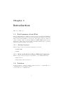
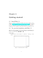
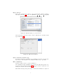
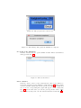
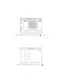
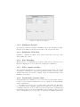
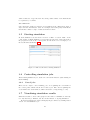
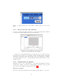
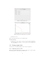
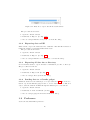
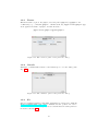
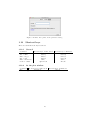
Flint 1.2: The User Guide
Flint project
February 27, 2015
Abstract
This document describes how to use Flint 1.2. Readers also find some OSspecific notes and trouble-shooting techniques which users would like to know
when using Flint 1.2.
Contents
1 Introduction
1.1 Brief summary about Flint . . . .
1.1.1 Markup languages . . . . .
1.1.2 Solver methods for ordinary
1.2 Notation . . . . . . . . . . . . . . .
.
.
.
.
3
3
3
3
3
2 Getting started
2.1 Install Flint 1.2 . . . . . . . . . . . . . . . . . . . . . . . . . . . .
2.2 Try your first simulation with Flint 1.2 . . . . . . . . . . . . . . .
4
4
4
. . . . . . . . . . . . .
. . . . . . . . . . . . .
differential equations .
. . . . . . . . . . . . .
3 Graphical User Interface
3.1 Launching Flint . . . . . . . . . . . . . . .
3.2 Quitting Flint . . . . . . . . . . . . . . . .
3.3 Loading models . . . . . . . . . . . . . . .
3.4 Configuring simulation tasks . . . . . . . .
3.4.1 Integration method . . . . . . . . .
3.4.2 Simulation Length . . . . . . . . .
3.4.3 Simulation Time Step . . . . . . .
3.4.4 Data Sampling . . . . . . . . . . .
3.4.5 Select output variables . . . . . . .
3.4.6 Parametrize constant values . . . .
3.5 Starting simulation . . . . . . . . . . . . .
3.6 Controlling simulation jobs . . . . . . . .
3.6.1 Cancel jobs . . . . . . . . . . . . .
3.7 Visualizing simulation results . . . . . . .
3.7.1 Choose abscissa and ordinates . .
3.7.2 Configuration for gnuplot . . . . .
3.8 Saving output data . . . . . . . . . . . . .
3.8.1 Exporing data as CSV . . . . . . .
3.8.2 Exporting data as ISD . . . . . . .
3.8.3 Exporting all data into a directory
3.8.4 Sending data to a Garuda gadget .
3.9 Preference . . . . . . . . . . . . . . . . . .
3.9.1 Plotter . . . . . . . . . . . . . . . .
3.9.2 Garuda . . . . . . . . . . . . . . .
3.9.3 K3 . . . . . . . . . . . . . . . . . .
3.10 Shortcut keys . . . . . . . . . . . . . . . .
3.10.1 General . . . . . . . . . . . . . . .
1
.
.
.
.
.
.
.
.
.
.
.
.
.
.
.
.
.
.
.
.
.
.
.
.
.
.
.
.
.
.
.
.
.
.
.
.
.
.
.
.
.
.
.
.
.
.
.
.
.
.
.
.
.
.
.
.
.
.
.
.
.
.
.
.
.
.
.
.
.
.
.
.
.
.
.
.
.
.
.
.
.
.
.
.
.
.
.
.
.
.
.
.
.
.
.
.
.
.
.
.
.
.
.
.
.
.
.
.
.
.
.
.
.
.
.
.
.
.
.
.
.
.
.
.
.
.
.
.
.
.
.
.
.
.
.
.
.
.
.
.
.
.
.
.
.
.
.
.
.
.
.
.
.
.
.
.
.
.
.
.
.
.
.
.
.
.
.
.
.
.
.
.
.
.
.
.
.
.
.
.
.
.
.
.
.
.
.
.
.
.
.
.
.
.
.
.
.
.
.
.
.
.
.
.
.
.
.
.
.
.
.
.
.
.
.
.
.
.
.
.
.
.
.
.
.
.
.
.
.
.
.
.
.
.
.
.
.
.
.
.
.
.
.
.
.
.
.
.
.
.
.
.
.
.
.
.
.
.
.
.
.
.
.
.
.
.
.
.
.
.
.
.
.
.
.
.
.
.
.
.
.
.
.
.
.
.
.
.
.
.
.
.
.
.
.
.
.
.
.
.
.
.
.
.
.
.
.
.
.
.
.
.
.
.
.
.
.
.
.
.
.
.
.
.
.
.
.
.
.
.
.
.
.
.
.
.
.
.
.
.
.
.
.
.
.
.
.
.
.
.
.
.
.
.
.
.
.
.
.
.
.
.
.
9
9
9
9
9
9
10
10
10
10
10
12
12
12
12
13
13
15
15
16
16
16
16
17
17
17
18
18
3.10.2 At the plot window . . . . . . . . . . . . . . . . . . . . . .
4 Command Line Interface
4.1 Launching Flint . . . . . . . . . . . . . . .
4.1.1 Invocation with no arguments . . .
4.1.2 Invocation with filenames . . . . .
4.2 Showing help . . . . . . . . . . . . . . . .
4.2.1 Synopsis . . . . . . . . . . . . . . .
4.3 Running a simulation: the headless mode
4.3.1 Synopsis . . . . . . . . . . . . . . .
2
.
.
.
.
.
.
.
.
.
.
.
.
.
.
.
.
.
.
.
.
.
.
.
.
.
.
.
.
.
.
.
.
.
.
.
.
.
.
.
.
.
.
.
.
.
.
.
.
.
.
.
.
.
.
.
.
.
.
.
.
.
.
.
.
.
.
.
.
.
.
.
.
.
.
.
.
.
.
.
.
.
.
.
.
.
.
.
.
.
.
.
18
19
19
19
19
19
19
20
20
Chapter 1
Introduction
Welcome to Flint 1.2.
1.1
Brief summary about Flint
Flint can run simulations of multi-level physiological models written in PHML. It
means that Flint parses given models, performs numerical analysis for their simulation, and renders simulation outcome into a line graph on the plot window’s
canvas. Likewise, Flint can handle SBML and SBML-PHML hybrid models.
Furthermore, Flint offers a plug-in feature with which different types of plotting
applications such as gnuplot are available.
1.1.1
Markup languages
Flint 1.2 supports the following three languages for models:
• PHML/ISML
• SBML
1.1.2
Solver methods for ordinary differential equations
Flint 1.2 supports the following two algorithms to solve ODEs numerically:
• Euler method
• Runge-Kutta 4th-order method
1.2
Notation
In this document, a sentence starting with $ describes a command line in a
command shell on your system, such as
$ echo this is a command line.
3
Chapter 2
Getting started
2.1
Install Flint 1.2
Flint project makes both Windows and Mac OS X version of Flint 1.2 freely
available at http://physiodesigner.org/simulation/flint/. The .dmg archive
for Mac OS X contains Flint’s application bundle, named “Flint.app”; extracting it and copying it into your favorite path is all you have to do for installation.
For Windows, double-clicking the .msi package will start the installation process.
2.2
Try your first simulation with Flint 1.2
This section describes a simple procedure with Flint 1.2 to run a simulation of a
sample model “HodgkinHuxley 1952 neuron model.phml”, which is distributed
as part of the PhysioDesigner installation.
Launch Flint
To launch Flint, double-click flint.exe on Windows, or Flint.app on Mac
OS X.
Figure 2.1: The initial window of Flint.
4
Open a model
In the “File” menu, select “Open” to choose a model file. Then you will see
a file dialog like Fig. 2.2. Select “HodgkinHuxley 1952 neuron model.phml”
Figure 2.2: The file dialog to open a model.
in the file dialog, and click “Open” button. Then the model window will
appear like Fig. 2.3.
Figure 2.3: The model window.
Choose duration and time step
Specify the duration of simulation in “Simulation Length” and the time
step length of the simulation in “Simulation Time Step” optionally.
Run a simulation
Click the “Run” button to start a simulation.
Once simulation started running, the progress bar will appear in the control panel in the right side like Fig. 2.4, and both “Cancel” (with the cross
mark) and “Detail” buttons will be enabled.
Wait until a message dialog shows up to tell that the simulation completed.
5
Figure 2.4: The progress bar for the model.
Figure 2.5: The message dialog says the simulation completed.
See detail of the simulation
Click the “Detail” button to get the simultion result. Then a detail window
will appear like Fig. 2.6.
Figure 2.6: The detail window.
Select ordinates
Click the “View” button on the detail window, then a plot window to
render line graphs about the simulation result, like Fig. 2.7. Drag a name
card “V” from the variable list, and drop it into the right axis field labelled
Y1. Soon the corresponding line graph will appear on the canvas, like
Fig. 2.8. At the same time you can also pick up another name “I Na”
from the list, moving it into the left axis field labelled Y2, like Fig. 2.9.
6
Figure 2.7: The plot window.
Figure 2.8: The plot window with “V” on Y1.
Plot a line graph with gnuplot
Push button “Plot” to draw the line graph about “V” and “I Na” with
gnuplot. Soon a gnuplot window will pop up like Fig. 2.10.
7
Figure 2.9: The plot window with “V” on Y1 and “I Na” on Y2.
Figure 2.10: Line graph by gnuplot about “V” and “I Na”.
8
Chapter 3
Graphical User Interface
Flint 1.2 comes with a graphical user interface out of the box. This chapter
explains features of the GUI and how to use them.
3.1
Launching Flint
On Windows, double-clicking “flint.exe” in the start menu starts Flint. On Mac
OS X, double-clicking “Flint.app” works similarly.
3.2
Quitting Flint
To quit Flint, use the menu “File”→“Exit”.
3.3
Loading models
Flint must load models before running simulations for them. Users tell Flint
which model should be loaded by opening the model file. Loading a model
can fail due to some reasons; for example, it may fail if the model file contains
an error or unsupported elements. An error dialog will display a diagnosis
message when loading a model fails. Once loading a model successfully, the
model window shows up and stays in the main window until closed.
3.4
Configuring simulation tasks
Before starting simulations for a loaded model, users may want to configure them
in terms of numerical integration, simulation time, output data, and parameters.
3.4.1
Integration method
Users have to choose a solver method for ordinary differential equations at the
“Integration method” combobox.
9
Figure 3.1: The model window.
3.4.2
Simulation Length
Users must specify the total length of simulation time at the “Simulation Length”
field; the given number is interpreted in terms of the selected time unit.
3.4.3
Simulation Time Step
Similarly to “Simulation Length”, users can specify the time step at the “Simulation Time Step” field.
3.4.4
Data Sampling
This setting is for determining how often the result data are written in. Note
that the sampling rate does not affect the calculation for simulation.
3.4.5
Select output variables
Before starting simulations for a loaded model, users may want to choose limited number of variables for output among available variables. Filtering output
variables will reduce the burden of writing output, and thus may improve the
simulation performance.
3.4.6
Parametrize constant values
By default, Flint run a simulation job for a loaded model. At the same time it is
possible to run a bunch of simulations at once for a single model with different
values of parameters.
A parameter is bound to a set of possible values, called value-set. The whole
set of possible tuples of multiple parameters is defined as a cartesian product
of multiple value-sets. If users define value-sets and use them, then Flint will
run as many jobs for the model as cardinality of the cartesian product. In other
words, each simulation job corresponds to a value tuple for multiple parameters.
10
Figure 3.2: The “Output Variables” panel.
Users can see and modify parametrization of constant elements in a loaded
model, such as the initial values of ordinary differential equations and values of
static-parameters of PHML, at the “Parameters” panel.
The table at the “Parameters” consists of each row corresponding to a constant element in the model; the “Expression” field of the row accepts a formula
(in an infix notation) defining the parametrized value of the constant element.
(a) a of type enum
(b) b of type interval
Figure 3.3: Editing value-sets in the “Define value set” window.
Define a value-set
In order to define or modify value-sets, push button “Define value set” at first.
Then a window will pop up. It allows users to define new value-set, see existing
value-sets, and modify them.
There are two types of value-sets: enum and interval. For a value-set of type
enum, each of possible values must be specified. On the other hand, only the
lower and upper (both inclusive) of a range of values with a step are required to
11
define a value-set of type interval. Note that possible values of an enum should
be separated by a comma.
Use value-sets
Once users have defined a value-set, it is available in the “Expression” field of
any row in the “Parameters” table. For example, users can specify a+2*b in the
field if there exists a couple of value-set named a and b.
3.5
Starting simulation
To start simulation, use the menu “Control”→“Run” or button “Run” on the
control panel. It kicks simulation jobs for all loaded models. Users can monitor
the progress in total on the control panel, as well as the one for a single job on
the detail windows like Fig. 3.4.
Figure 3.4: The detail window during simulation.
3.6
Controlling simulation jobs
After starting simulation jobs, users can control them instead of just waiting for
them finishing.
3.6.1
Cancel jobs
There are two ways to cancel running jobs; one is pushing the cross mark on
the control panel, which cancels all of related jobs. The other is pushing the
cross mark at the detail window, which cancels the corresponding job only.
3.7
Visualizing simulation results
Flint has a feature to show a line graph for the result of a simulation on the fly,
not only after its job finished, but also int the middle of ongoing simulation.
From the detail window, users can display the plot window by clicking button
“View” for each simulation job.
12
Figure 3.5: The progress bar / cross mark / “Detail” button on the control
panel.
3.7.1
Choose abscissa and ordinates
In order to draw a line graph, users have to specify the abscissa and ordinates
by drag-and-dropping variables from the left side frame.
Figure 3.6: Selecting V as a Y1 ordinate.
If there are so many variables that some of them scroll out on a frame, a scroll
bar appears on the left edge of the frame. Besides scrolling them by wheeling
with mouse, especially on the left side frame, the focus can jump to a variable
by typing an alphabet key (i.e., [A-z]) which specifies the first character of the
variable’s name.
3.7.2
Configuration for gnuplot
Pushing the “Plot” button calls gnuplot to draw a line graph with the specified
abscissa and ordinates. Users have to install gnuplot in advance, and to specify
the location of the gnuplot executable (see section 3.9).
Options for gnuplot
Users can control the following options for gnuplot in Tab “Range” or “Legend”:
13
• Minimum and/or maximum value(s) for the abscissa (X) and/or ordinates
(Y 1/Y 2)
• Labels for the abscissa (X) and/or ordinates (Y 1/Y 2)
• With or without the title
These will be enabled on next time plotting.
Figure 3.7: The “Target” tab.
Figure 3.8: The “Range” tab.
Writing the line graph to a file
It is possible to make gnuplot write the line graph to some file, as follows:
• choose Tab “Target”.
• check the “file” button.
• select a file format and path to be written.
14
Figure 3.9: The “Legend” tab.
Figure 3.10: The line graph generated by gnuplot.
• push button “Plot”.
Then a dialog will inform users of the resulting status.
Trouble shooting
• Pushing button “Plot” with no response, check the gnuplot initialization
file to load. It is called .gnuplot on Unix and Mac OS X, and GNUPLOT.INI
on other systems.
3.8
Saving output data
Users may save the resulting simulation data for later investigation.
3.8.1
Exporing data as CSV
Flint can export the result data into a CSV file. The header column contains
the variable names as well as their unit name if any.
15
Figure 3.11: Buttons to export data in the detail window.
The procedure is as follows:
1. Open the “Detail” window
2. Push button “Export” (see Fig. 3.11)
3. Choose a target filename ending with .csv in the file dialog.
3.8.2
Exporting data as ISD
Flint can also export the result data into a ISD file. The ISD file format is a
binary file format for preserving multi-variate data.
The procedure is as follows:
1. Open the “Detail” window
2. Push button “Export” (see Fig. 3.11)
3. Choose a target filename not ending with .csv in the file dialog.
3.8.3
Exporting all data into a directory
It is sometimes useful to export all data for simulation jobs into a directory.
The procedure is as follows:
1. Open the “Detail” window
2. Push button “Export all” (see Fig. 3.4)
3. Choose a target directory in the file dialog.
3.8.4
Sending data to a Garuda gadget
If Flint is enabled for the Garuda protocol (see subsection 3.9.2 about how to
turn it on), and an Garuda gadget is able to receive data in CSV or ISD, it is
easy to send the result from Flint through the Garuda protocol as follows:
1. Open the “Detail” window
2. Push button “Send via Garuda” (see Fig. 3.4)
3. Choose a target gadget from the list in the next dialog.
3.9
Preference
Users can customize Flint’s preference.
16
3.9.1
Plotter
This is an advanced option. For gnuplot, select the path of gnuplot (or pgnuplot.exe
on Windows), e.g., “/usr/bin/gnuplot”. On Mac OS X, say, /Applications/gnuplot.app
as an application bundle of gnuplot, its value should be
/Applications/gnuplot.app/bin/gnuplot.
Figure 3.12: The “Plotter” panel on the preference dialog.
3.9.2
Garuda
Turning it on makes Flint enabled for the Garuda protocol on the desktop, like
Fig. 3.13.
Figure 3.13: The “Garuda” panel on the preference dialog.
3.9.3
K3
Instead of runnsing simulation with Flint, submitting a loaded model to Flint K3
(http://flintk3.unit.oist.jp/) for simulation is also possible. In order to
enable the feature, users must specify its account information at this preference
in advance, like Fig. 3.14.
17
Figure 3.14: The “K3” panel on the preference dialog.
3.10
Shortcut keys
There are useful shortcut keys as follows:
3.10.1
General
Command
File → Open
File → Exit
Edit → Copy
File → Cut
Edit → Preference
Control → Run
3.10.2
Shortcut keys on Mac OS X
Cmd+O
Cmd+Q
Cmd+C
Cmd+X
Cmd+,
Option+R
Shortcut keys on Windows
Ctrl+O
Ctrl+Q
Ctrl+C
Ctrl+X
Ctrl+,
Alt+R
At the plot window
Command
Plot
Shortcut keys on Mac OS X
Option+P
18
Shortcut keys on Windows
Alt+P
Chapter 4
Command Line Interface
Flint 1.2 allows users to run a simulation in a command shell.
4.1
4.1.1
Launching Flint
Invocation with no arguments
It is possible to launch Flint with the command open(1) of Mac OS X as follows:
$ open Flint.app
Note that it does nothing but launches the graphical user interface of Flint. In
a cmd session on Windows,
$ flint.exe
has the similar effect.
4.1.2
Invocation with filenames
If filenames of models are given in the command line on Windows:
$ flint.exe model1 model2 ...
then Flint tries to open them immediately after launching the GUI.
4.2
Showing help
Specifying -help in the command line shows the help message.
4.2.1
Synopsis
On Windows:
$ flint.exe -help
19
4.3
Running a simulation: the headless mode
Specifying -headless in the command line enable the headless mode, which
runs a simulation of given model with the default configuration.
4.3.1
Synopsis
On Windows:
$ flint.exe -headless input output [-e file] [-g n] [-s file]
Load a model at input, simulation it with the default configuration, and leave
the result at output. The following suboptions are available:
-e file
save error messages during simulation as file.
-g n
specify a sampleing rate i.e. 1 output per n step.
-s file
specify output variables with file.
20