Download User Manual - PhysioDesigner

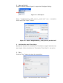
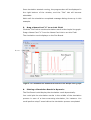
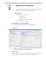
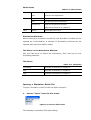
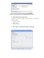
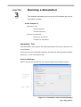
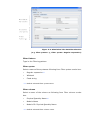
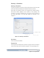
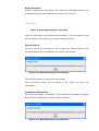
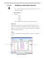
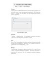
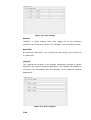
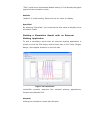
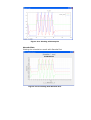
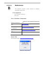
User Manual
Flint
Contents
WELCOME TO FLINT .................................................................. 4
Brief Introduction ....................................................... 4
Getting Started ........................................................... 4
Launch Flint ................................................................................ 4
Open a Mode ................................................................................ 4
Set Duration and Time Step ....................................................... 4
Run ............................................................................................... 4
Drag a Name Card “V” to the Axis Field .................................... 4
Plotting a Simulation Result in Dynamic .................................. 4
BEGINNING A SIMULATION ....................................................... 7
The Elements on the Flint Window .......................... 7
Window Menu .............................................................................. 7
Simulation Window ..................................................................... 7
Tab Menu on the Simulation Window ........................................ 7
Opening a Simulation Model File .............................. 7
RUNNING A SIMULATION ........................................................ 10
Simulation Tab .......................................................... 10
General Settings ........................................................................ 10
Variable Selection ...................................................................... 10
Running a Simulation ............................................... 10
Starting a Simulation ................................................................ 10
Complete a Simulation .............................................................. 10
2
PLOTTING A SIMULATION RESULT........................................ 16
Plot Tab .................................................................... 16
Track .......................................................................................... 16
Target ......................................................................................... 16
Range.......................................................................................... 16
Legend ........................................................................................ 16
Plot a Simulation Result with an External Plotting
Application ............................................................... 16
LOGS .......................................................................................... 23
Log Tab ..................................................................... 23
PREFERENCE SETTINGS......................................................... 25
Preference ................................................................. 25
Plotter......................................................................................... 25
New Plotter Add / Edit Plotter Info .......................................... 25
Delete Plotter ............................................................................. 25
KEY EQUIVALENTS .................................................................. 27
List of Key Equivalents ............................................ 27
REFERENCES............................................................................ 28
List of Software Components .................................. 28
About Flint ................................................................ 28
3
Welcome to Flint
CHAPTER
1
This chapter introduces you to Flint, a physiological function
model simulator and its basic usage.
In the Chapter 1
Brief Introduction
Getting Started
Launch Flint
Open a Mode
Set Duration and Time Step
Run
Drag a Name Card “V” to the Axis Field
Plotting a Simulation Result in Dynamic
Brief Introduction
Flint is a GUI based application for a simulation of the multi-level
physiological models written in insilicoML (ISML).
Flint parses models
and performs numerical calculations in its simulation processes, and
Flint dynamically renders a simulation outcome into a line graph on the
Plot Board window. Likewise, Flint can handle SBML and SBML-ISML
hybrid models.
Furthermore, Flint offers an extendable function to plot simulation
results with different types of plotting applications.
Getting Started
Here in this section describes a simple procedure how to run a
simulation with Flint.
This procedure uses “HodgkinHuxley_1952_neuron_model.isml” as a
simulation sample model.
1.
Launch Flint:
To launch Flint, double-click the flint.exe file (or Flint.app with Mac
OSX).
4
2.
Open a Model:
In the File menu, select “Open” to open the File Open Dialog.
Figure 1-1: File>Open
Select “HodgkinHuxley_1952_neuron_model.isml” as a simulation
model and Click “Open” button.
Figure 1-2: Open “HodgkinHexley_1952_neruon_model.isml”
3.
Set Duration and Time Step:
Specify the duration of simulation in “Simulation Length” and the time
step length of the simulation in “Simulation Time Step” in an option.
4.
Run:
Click the “Run” button to start the simulation.
Figure 1-3: Set Duration and Time Step
5
Once simulation started running, the progress bar will be displayed in
the right bottom of the window, and the “Plot” tab will become
selectable.
Wait until the simulation completed message dialog shows up in this
example.
5.
Drag a Name Card “V” to an Axis Field:
Click the “Plot” tab to see the simulation result in the simple line graph.
Drag a Name Card “V” from the Name Card List to an Axis Field.
The simulation result displays on the Plot Board.
Figure 1-4: Visualize the Simulation Result in the Simple Line-graph
6.
Plotting a Simulation Result in Dynamic:
The Plot Board could display the simulation result dynamically.
You could plot the simulation results in the middle of the simulation
process in case of a time-consuming simulation, for instance. You
could perform step 5 even before the simulation process completed.
6
CHAPTER
2
Beginning a Simulation
This chapter discusses about basic elements in the Flint and
opening a model file for beginning a simulation.
In the Chapter 2
The Elements on the Flint Window
Window Menu
Simulation Window
Tab Menu on the Simulation Window
Opening a Simulation Model File
The Elements on the Flint Window
This section describes the elements on the Flint window.
Figure 2-1: Elements on the Flint Window
Window Menu:
Located at the top of the Flint window, the window menu gives
one-click access to commonly use the following menu items.
7
Menu Items
Table 2-1: Menu Items
File
Edit
Open
Open a simulation model
Exit
Quit the Flint application
Copy
Copy the log test to clip board
Cut
Cut the log text to clip board
Preference
Open the Preference window
Describe its features in Chapter 6
Help
about…
Show about the Flint
Simulation Windows:
When selecting a simulation model file, the Simulation window will be
opened as a sub-window. A number of Simulation windows can be
opened with each simulation model.
Tab Menu on the Simulation Window:
Use the Tab menu to select the Simulation, Plot, and Log for the
simulating features.
Tab Items
Table 2-2: Tab Items
Simulation
Describe its features in Chapter 3
Plot
Describe its features in Chapter 4
Log
Describe its features in Chapter 5
Opening a Simulation Model File
To open a simulation model file with the Open command:
1.
Choose “Open” from the File menu.
Figure 2-2: Choose File>Open
Flint displays a standard File Open dialog:
8
Figure 2-3: File Open dialog (e.g. selecting bvp_pulse.isml)
2.
Select the file you want to open.
Currently the following Markup Language files are available to
represent models:
•
insilicoML (.isml)
•
SBML (.sbml)
•
CellML (.cellml)
3.
Click “Open” to open the simulation model file.
The Simulation Window of selected model displays:
Figure 2-4: Simulation Window (e.g. bvp_pluse)
9
CHAPTER
3
Running a Simulation
This chapter discusses how to use the Simulation tab on the
Simulation window.
In the Chapter 3
Simulation Tab
General Settings
Variable Selection
Running a Simulation
Starting a Simulation
Complete a Simulation
Simulation Tab
The Simulation tab, it gives the setting features of how you want to run
a simulation.
There are two secondly tab windows, the General Settings and Variable
Selection, in the Simulation tab.
General Settings:
Use to set up the Numerical Simulation Method and Data Output.
Figure 3-1: Simulation Tab>General Settings
(e.g. bvp_pluse)
10
Numerical Simulation Method
•
Numerical Integration Method*1: Select a name of the method
in a popup menu.
•
Currently the following two algorithms are available to solve
ODEs*2 numerically.
Ø
Euler Method
Ø
Runge-Kutta 4th Order Method
*1: By default, the Numerical Integration Method is set depending upon the
selected simulation model.
*2: ODEs: Ordinary Differential Equations
•
Simulation Length*3: Type in the simulation length with the
selection of the unit in one of four, second, millisecond,
microsecond, or nanosecond.
*3: By default, the unit of the Simulation Length is set depending upon the
selected simulation model.
•
Simulation Time Step*4: Type in the simulation time step with
the selection of the unit in one of four, second, millisecond,
microsecond, or nanosecond.
*4: By default, the unit of the Simulation Time Step is set depending upon
the selected simulation model.
Data Output
•
Data Sampling: Set how many steps for every data sampling.
•
Enable the labeled format (.dat): Check to generate the
simulation result file with .dat extension, in addition to the one
with .csv extension.
Variable Selection:
Select the variables for simulating the model. Use the Filter pattern,
Filter syntax, and Filter column to filter the variables for the simulation
you wish to run. The filtered variables are displayed in the Enabled
Variables section.
11
Figure 3-2: Simulation Tab>Variable Selection
(e.g. Filter pattern: y, Filter syntax: Regular expression)
Filter Pattern
Type in the Filtering pattern.
Filter syntax
Select a name of the syntax as following from Filter syntax combo box.
•
Regular expression*5
•
Wildcard
•
Fixed string
*5: Default selected Filter syntax name
Filter column
Select a name of the column as following from Filter column combo
box.
•
Physical Quantity Name*6
•
Module Name
•
Module ID: Physical Quantity Name
*6: Default selected Filter column name
12
Running a Simulation
Starting a Simulation:
To start a simulation is simply to click the Run button at the lower part
of the both General Settings and Variable Selection windows.
Soon after the simulation starts, the Progress bar, Suspend button,
and Cancel button appears at the bottom of the window. The
simulation in progress is displayed as a line graph on the Plot Board at
the Track tab window. The Track tab window will describe in the
Chapter 4.
Figure 3-3: Starting a Simulation
Run button
Click to start the simulation.
Progress bar
The Progress bar indicates the simulation progress with the simulation
model name and overall simulation progress in the percentage (%).
Figure 3-4: Progress Bar
13
Suspend button
Click to suspend the simulation. By clicking the Suspend button, the
message dialog will be displayed to confirm your action.
Figure 3.5!!!
Figure 3-5: Message Dialog for Suspend
Click the OK button to suspend the simulation. The simulation result
will be saved in the file(s) up until the suspend action.
Cancel button
Click to cancel the simulation. By clicking the Cancel button, the
message dialog will be displayed to confirm your action.
Figure 3-6: Message Dialog for Cancelation
Click the OK button to cancel the simulation.
The simulation result will be saved in the file(s) up until the
cancelation.
Complete a Simulation:
When the simulation completes, the Simulation Complete message
dialog will be displayed to confirm the completion.
Figure 3-7: Message Dialog for Completion
14
Click the OK button to end the simulation process.
How you perform the simulation, the simulation result will be saved in
the file(s), .csv and optionally .dat extension files, to the same
directory where your simulation model file is located.
15
Plotting a Simulation Result
CHAPTER
4
This chapter discusses how to use the Plot tab on the
Simulation window.
In the Chapter 4
Plot Tab
Track
Target
Range
Legend
Plot a Simulation Result with an External Plotting Application
Plot Tab
The Plot tab, it gives the visualizing features of a simulation result.
There are four secondly tab windows, the Track, Target, Range, and
Legend, in the Plot tab; these secondly tab windows are disabled
before starting the simulation.
Track:
The Track tab window is the simple display window of a simulation
result.
Figure 4-1: Plot>Track
16
Variable List Box (describe as “Name Card List” in Chapter 1)
After starting the simulation, all variables (describe as “Name Card” in
Chapter 1), corresponding to physical quantities, of the simulating
model are displayed in the Variable List Box.
Left and Right Ordinate Boxes
Drag and drop the variable(s) from the Variable List Box to the Left or
Right Ordinate Box for plotting the simulation result. You could place
the multiple variables in these boxes.
Abscissa Box
The Abscissa Box takes only one variable and is normally the time axis
for plotting the simulation result.
You could change the time axis to the Left or Right Ordinate Box.
The time axis switches automatically by dragging a variable from the
Ordinate Box and by dropping to the Abscissa Box.
Plot Board
The Plot Board displays a line graph of the simulation result in progress
on the real axis. During the simulation, the Plot Board displays the
graph of dynamic simulation results corresponding to the disposed
variables on the Ordinate and Abscissa Boxes.
The simulation results in the variables of the Left Ordinate Box
indicated with the graph in red, and the ones of the Right Ordinate Box
is indicated with the graph in blue.
17
Figure 4-2: Plotting a Simulation Result on the Plot Board
(e.g. bvp_pluse)
Right-click (Control-click for Mac OSX) on the Plot Board to display the
contextual menus. The contextual menu includes the view control
commands and export commands.
View control commands
•
Zoom in
•
Zoom out
•
Reset view
Export commands
•
Export image…
•
Export image in typical image file
formats: PNG, JPEG, EPS, WBMP, SVG,
BMP, GIF, and PDF
•
Print…
Figure 4-3: Contextual Menu
on the Plot Board
Status
By click a variable in the Variable List Box, Left Ordinate Box, Right
Ordinate Box, and Abscissa Box, the Status displays its variable name,
maximum and minimum values, and the overall simulation progress in
the percentage (%).
18
Figure 4-4: Status of the Variable x
Target:
The Target tab window is the redirect parameter setting window of a
simulation result for an external plotting application. The Target tab
window is currently only compatible with the Gunplot of the external
plotting application.
Figure 4-5: Plot>Target
Window
“Window” is default setting. This setting will output the simulation
result to the external plotting application window.
File
When “File” is selected, the simulation result will be exported as a file
through the external plotting application. You could set the export file
path and file format as PDF, PNG, or EPS.
Range:
The Range tab window is the parameter settings of X, Y, and Y2 axes
ranges, for an external plotting application.
The Range tab window is
currently only compatible with the Gunplot of the external plotting
application.
19
Figure 4-6: Plot>Range
Default
“Default” is initial setting. Each axis range will be set between
minimum and maximum values of a variable in the simulation result.
Specified
By selecting “Specified”, you could set the axis range, from minimum
to maximum.
Legend:
The Legend tab window is the display parameter settings of graph
legend for an external plotting application. The Legend tab window is
currently only compatible with the Gunplot of the external plotting
application.
Figure 4-7: Plot>Legend:
Title
20
“Title” check box is checked as default setting. It is to display the graph
legend of the simulation result.
Default
“Default” is initial setting. Each axis has no name to display.
Specified
By selecting “Specified”, you could set the axis name to display in the
simulation result.
Plotting a Simulation Result with an External
Plotting Application
To plot a simulation result with an external plotting application is
simply to click the Plot button at the lower part of the Track, Target,
Range, and Legend windows on the Plot tab.
Figure 4-8: Plot Board
insilcoSIM currently supports two external plotting applications,
Gnuplot and Garuda Plot.
Gnuplot:
Plotting the simulation result with Gnuplot.
21
Figure 4-9: Plotting with Gnuplot
Garuda Plot:
Plotting the simulation result with Garuda Plot.
Figure 4-10: Plotting with Garuda Plot
22
CHAPTER
5
Logs
This chapter discusses how to use the Log tab on the
Simulation window.
In the Chapter 5
Log Tab
Log Tab
The Log tab is to displays simulation logs.
Figure 5-1: Log
Description of the simulation logs
23
By using "Copy" command on the Edit menu, you could copy the
simulation logs from the display window
to
the
clipboard.
Using
the
"Cut"
command in a similar way, you could cut
the simulation logs.
Figure 5-2: Copy and Cut
24
Preference Settings
CHAPTER
6
This chapter discusses how to use the “Preference” settings
on the Edit menu.
In the Chapter 6
Preference
Plotter
New Plotter Add / Edit Plotter Info
Delete Plotter
Preference
The Preference is for set up the external plotting applications.
Selecting
the
“Preference”
command on the Edit menu opens
the Preference window.
Figure 6-1: Edit>Preference
Figure 6-2: Preference Window
Plotter
Select a name of the external plotting application from Plotter combo
box. You could also switch to the other plotters running the simulation.
Figure 6-3: Selecting an External Plotter
25
New Plotter Add / Edit Plotter Info
Click the “New Plotter Add” button to register an external plotting
application.
Type following input items, and click OK to register the new Plotter.
•
Plotter Name: New plotter’s name
•
Plotter Path: Set a path to the plotter executable file
•
External Setting:
•
Check to enable to use the Track, Range, and Legend on the Plot
tab
Click the “Edit Plotter Info” button to change an external plotting
application settings. Setting items and operation are the same as
registering new plotter.
Figure 6-4: New Plotter Add / Edit Plotter Info
Delete Plotter
Click the “Delete Plotter” button to remove the external plotting
application selected in “Plotter”.
The message dialog will be displayed to confirm your action.
Figure 6-5: Delete Plotter
26
Key Equivalents
APPENDIX
A
This appendix provides a quick reference for pre-assigned
shortcut keys that are available from Flint’s user interface.
In the Appendix A
List of Key Equivalents
List of Key Equivalents
For MS Windows
Table A-1: Shortcut Keys for MS Windows
Key
Command
Ctrl-O
File: Open
Ctrl-Q
File: Exit
Ctrl-C
Edit: Copy
Ctrl-X
Edit: Cut
Ctrl-,
Edit: Preference
Ctrl-H
Help: about…
Alt-R
Simulation: Run
Alt-P
Plot: Plot
For Mac OSX
Table A-2: Shortcut Keys for Mac OSX
Key
Command
Cmd-O
File: Open
Cmd-Q
Flint: Quit Flint
Cmd-C
Edit: Copy
Cmd-X
Edit: Cut
Cmd-,
Flint: Preference
Cmd-H
Help: about…
Alt-R
Simulation: Run
Alt-P
Plot: Plot
27
References
APPENDIX
B
This appendix provides a quick reference of software
component used in Flint.
In the Appendix B
List of Software Components
About Flint
List of Software Components
Table B-1: List of Software Components
Software Component
URI
Java
http://java.com/
1.6
GRAL
http://trac.erichseifert.de/gral/
0.9-SNAPSHOT
Protocol Buffers
http://code.google.com/p/protobuf/
2.4.1
About Flint
Flint project site URI: http://www.physiodesigner.org/
Figure B-1: Help>About…
28