1
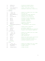
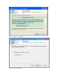
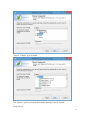
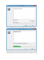
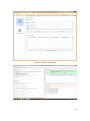
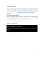
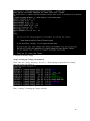
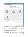
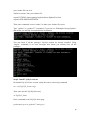
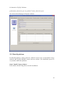
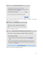
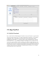
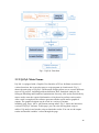
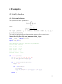
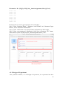
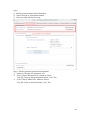
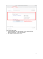
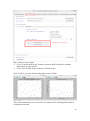
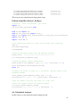
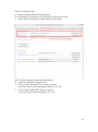
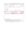
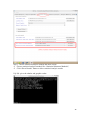
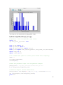
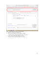
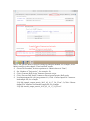
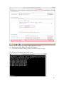
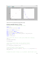
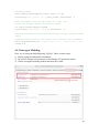
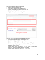
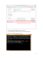
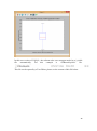
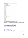
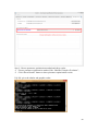
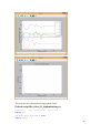
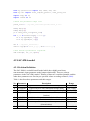
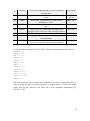
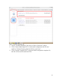
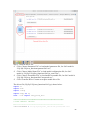
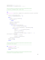
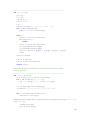
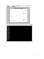
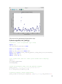
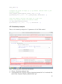
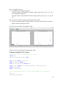
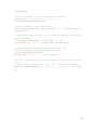
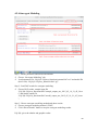
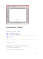
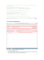
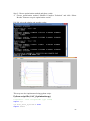
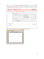
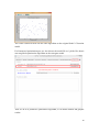
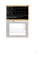
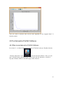
UQ-PyL User Manual (Version 1.1) Chen Wang ([email protected]) Qingyun Duan ([email protected]) Beijing Normal University Beijing, China 1 Table of Contents 1 Introduction .................................................................................................................................... 3 1.1 A Quick Start ....................................................................................................................... 3 1.2 Available UQ-PyL Capabilities ........................................................................................... 3 1.2.1 Design of Experiment .............................................................................................. 3 1.2.2 Statistical Analysis ................................................................................................... 3 1.2.3 Sensitivity Analysis .................................................................................................. 3 1.2.4 Surrogate Modeling.................................................................................................. 3 1.2.5 Parameter Optimization ........................................................................................... 4 1.3 Overview about functionality of the UQ-PyL package ....................................................... 4 2 Installation...................................................................................................................................... 6 2.1 Dependencies ...................................................................................................................... 6 2.2 Detailed Installation ............................................................................................................ 6 2.2.1 Windows platform .................................................................................................... 6 2.2.2 Linux platform ....................................................................................................... 14 2.2.3 MacOS platform ..................................................................................................... 20 3 Using UQ-PyL ............................................................................................................................. 25 3.1 UQ-PyL Flowchart ............................................................................................................ 25 3.2 UQ-PyL Main Frame ........................................................................................................ 26 4 Examples ...................................................................................................................................... 28 4.1 Sobol’ g-function............................................................................................................... 28 4.1.1 Problem Definition ................................................................................................. 28 4.1.2 Design of Experiment ............................................................................................ 29 4.1.3 Statistical Analysis ................................................................................................. 33 4.1.4 Sensitivity Analysis ................................................................................................ 38 4.1.5 Surrogate Modeling................................................................................................ 43 4.1.6 Parameter Optimization ......................................................................................... 48 4.2 SAC-SMA model .............................................................................................................. 52 4.2.1 Problem Definition ................................................................................................. 52 4.2.2 Design of Experiment ............................................................................................ 58 4.2.3 Sensitivity Analysis ................................................................................................ 61 4.2.4 Surrogate Modeling................................................................................................ 64 4.2.5 Parameter Optimization ......................................................................................... 66 4.3 Run simulation on surrogate model .................................................................................. 68 4.4 Use Interactive UQ-PyL Software .................................................................................... 72 4.4.1 How to run interactive UQ-PyL Software .............................................................. 72 4.4.2 How to use interactive UQ-PyL Software .............................................................. 73 2 1 Introduction 1.1 A Quick Start UQ-PyL (Uncertainty Quantification Python Laboratory) is a software platform for performing various uncertainty quantification (UQ) activities such as Design of Experiments (DoE), Statistical Analysis, Sensitivity Analysis (SA), Surrogate Modeling and Parameter Optimization. This document describes how to set up problems and use these UQ methods to solve them through UQ-PyL. The mathematics of those UQ methods can be found in the separate theory manual. We request that you cite the following paper when you report the results obtained by using the UQ-PyL software platform: C. Wang, Q. Duan, Charles H. Tong, (2015), UQ-PyL – A GUI platform for uncertainty quantification of complex models. Under review for Environmental Modeling & Software. 1.2 Available UQ-PyL Capabilities 1.2.1 Design of Experiment Full-Factorial design, Fractional-Factorial design, Plackett-Burman design, Box-Behnken design, Central-Composite design, Monte Carlo design, Latin Hypercube design (random, center, maxmin, center maxmin, correlate), Symmetric Latin Hypercube design, Improved Distributed Hypercube design, Sobol’ sequence, Halton sequence, Faure sequence, Hammersley sequence, Good Lattice Point. 1.2.2 Statistical Analysis Statistical moments, Confidence interval, Hypothesis test. 1.2.3 Sensitivity Analysis Morris One at A Time (MOAT), Derivative-based Global Sensitivity Measure (DGSM), Sobol’ Sensitivity Analysis, Fourier Amplitude Sensitivity Test (FAST), Metamodel-based Sobol’, Correlation analysis, Delta Moment-Independent Measure (Delta), Multivariate Adaptive Regression Splines (MARS) based sensitivity analysis. 1.2.4 Surrogate Modeling Generalized Linear Model (Ordinary Least Squares, Ridge Regression, Lasso, Least Angle Regression, LARS Lasso, Bayesian Regression, and Elastic Net), Regression 3 Tree, Random Forest, Nearest Neighbors, Support Vector Machine, Gaussian Process, MARS, Stochastic Gradient Descent. 1.2.5 Parameter Optimization Shuffled Complex Evolution (SCE), Dynamically Dimensional Search (DDS), Adaptive Surrogate Modeling based Optimization (ASMO), Particle Swarm Optimization (PSO), Simulated Annealing (SA), and Monte Carlo Markov Chain (MCMC). 1.3 Overview about functionality of the UQ-PyL package 1 __init__.py 2 DoE/ 3 __init__.py # Ensure all needed files are loaded 4 __main__.py # For GUI uses 5 box_behnken.py # Box-behnken design 6 central_composite.py # Central-composite design 7 fast_sampler.py # FAST sensitivity analysis design 8 faure.py # Faure design 9 ff2n.py # Factorial design 10 finite_diff.py # DGSM sensitivity analysis design 11 frac_fact.py # Factorial design 12 full_fact.py # Full Factorial design 13 GLP.py # Good Lattic Point design 14 halton.py # Halton Quasi-Monte Carlo design 15 hammersley.py # Hammersley Quasi-Monte Carlo design 16 lhs.py # Latin Hypercube design 17 monte_carlo.py # Monte Carlo design 18 morris_oat.py # Morris One at A Time design 19 plackett_burman.py # Plackett Burman design 20 saltelli.py # Sobol' sensitivity analysis design 21 sobol.py # Sobol' Quasi-Monte Carlo design 22 symmetric_LH.py # Symmetric Latin Hypercube design 23 analysis/ 24 __init__.py # Ensure all needed files are loaded 25 __main__.py # For GUI uses 26 confidence.py # Confidence Interval 27 correlations.py # Correlation analysis 28 delta.py # Delta sensitivity analysis 29 dgsm.py # DGSM sensitivity analysis 30 extended_fast.py # FAST sensitivity analysis 31 hypothesis.py # Hypothesis Test 4 32 moments.py # Statistics moments method 33 morris.py # MOAT sensitivity analysis 34 sobol_analyze.py # Sobol' sensitivity analysis 35 sobol_svm.py # Metamodel based sobol' sensitivity analysis 36 RSmodel/ 37 __init__.py # Ensure all needed files are loaded 38 __main__.py # For GUI uses 39 BayesianRidge.py # GLP-Bayesian Ridge regression 40 DT.py # Decision Tree regression 41 ElasticNet.py # GLP-Elastic Net regression 42 gp.py # Gaussian Process regression 43 kNN.py # k-nearest neighbor regression 44 LAR.py # GLP-LAR regression 45 Lars.py # GLP-Lars regression 46 Lasso.py # GLP-Lasso regression 47 MARS.py # MARS regression 48 OrdinaryLeastSquares.py # GLP-Ordinary Least Squares regression 49 RF.py # Random Forest regression 50 Ridge.py # GLP-Ridge regression 51 SGD.py # Stochastic Gradient Descent regression 52 SVR.py # Support Vector Machine regression 53 optimization/ 54 __init__.py # Ensure all needed files are loaded 55 __main__.py # For GUI uses 56 ASMO.py # ASMO optimization 57 DDS.py # DDS optimization 58 MCMC.py # Monte Carlo Markov Chain optimization 59 PSO.py # Particle Swarm Optimization 60 SA.py # Simulated Annealing optimization 61 SCE.py # Shuffled Complex Evolution optimization 62 util/ 63 __init__.py # Ensure all needed files are loaded 64 discrepancy.py # Compute discrepancy of design 65 spyderlib/ # Spyder package 66 spyderplugins/ # Spyder package 5 2 Installation 2.1 Dependencies UQ-PyL is an open-source package written in Python language. It runs on all major platforms (Windows, Linux, MacOS). It requires some pre-installed standard Python packages: Python version >= 2.7.6 Numpy >= 1.7.1 Scipy >= 0.16.0 Matplotlib >= 1.4.3 PyQt4 (If you use graphic user interface) Scikit-learn = 0.14.1 2.2 Detailed Installation 2.2.1 Windows platform For Windows platform, there is a software integrate Python and some common packages called Python(xy). It contains all the packages UQ-PyL needed. You can just install Python(xy) and UQ-PyL to run UQ analysis. Step 1. Install Python(xy) software. You can download “Python(xy)” from our website. Double click the Installation file to start installation. 6 Click “I Agree” to continue. Click “Next” to continue. 7 Choose “Custom” type to install. For “Python” option, you must check all the package UQ-PyL needed. “ PyQt 4.9.6-4 8 NumPy 1.8.0-5 Scipy 0.13.3-6 Matplotlib 1.3.1-4 Scikit-learn 0.14.1-4 (Please note: this one is not checked by default) ” Click “Next” to continue. Click “Next” to continue. 9 Click “Install”, then waiting for the installation process. After installation, you executable python.exe file will be C:\Python27\python.exe. All the package will be in the C:\Python27\Lib\site-packages directory. Step 2. Install UQ-PyL software Please download UQ-PyL Windows version, double click to run the installation file. 10 Choose the default directory D:\ or your own path, then click “unzip” to continue. After unzip, there will be two shortcut on the desktop, one is refer to UQ-PyL software main page, the other is refer to interactive version of UQ-PyL software. Double click the shortcuts can start the UQ-PyL software. If the shortcut doesn’t work, 11 please go to your install path, double click the “main.pyw” file or “main_interactive.pyw” file to start these. In UQ-PyL main page, you can do uncertainty quantification analysis through pull-down menus. In interactive version of UQ-PyL software, you can write python script to run uncertainty quantification analysis and can see output results and internal variables’ values through the software’s interface. UQ-PyL Splash Page 12 UQ-PyL Software Main Page Interactive UQ-PyL Software 13 2.2.2 Linux platform Canopy is a globally recommended Python distribution. It contains Python and 100+ common built-it packages. It also contains all the package UQ-PyL used in one software. So you can install Canopy for all the dependences UQ-PyL needed. Please go to the official website (https://www.enthought.com/products/canopy/) for more information. Step 1. Install Canopy software. Canopy is a commercial software. However, it provide free use for academic usage. If you use Canopy for education or academic, you can download canopy-1.5.5-full-rh5-64.sh from our website or from Canopy official website. After downloading, you should install Canopy by steps below: chmod 755 canopy-1.5.5-full-rh5-64.sh ./canopy-1.5.5-full-rh5-64.sh If you approve the license term, press Enter to continue 14 Type “yes” then press Enter to continue. Type the path you want to install Canopy, then press Enter to continue. 15 Complete to install Canopy. Step 2: Setting up Canopy environment Enter into the Canopy directory, for me is “/home/quanjp/swgfs/software/Canopy”, you can see the file inside it. Run “./canopy” to setting up Canopy software 16 Enter the Canopy environment directory, for me is “/home/quanjp/swgfs/software/Python”, click “Continue” to continue. Your python installation will in this directory. After that, a dialogue will display, Choose “Yes”, then click “Start using Canopy”. 17 In “Package Manager” section, you can check what packages in your Python library now. Actually, you can check your python installation in your python installation path. All files are in “YourPythonPath/User/” (for me is /home/quanjp/swgfs/software/Python/User/). The python executable file is in “YourPythonPath/User/bin/” and all the packages are installed in “YourPythonPath/User/lib/python2.7/site-packages/”. Step 3: Test your Python installation If you have multiple python environment, please specific one. Usually, modify 18 your .bashrc file can do it. Add two sentence into your .bashrc file: export PYTHON=/home/quanjp/swgfs/software/Python/User/bin export PATH=$PATH:$PYTHON: Then enter command “source .bashrc” to make your .bashrc file renew. Type “python” or “python2.7” command, if you can see “Enthought Canopy Python” that means you already accomplished the installation. You can check if all the packages UQ-PyL needed are already installed. Using “import” command, if no error messages that means you already have all the packages. Step 4. Install UQ-PyL software Download UQ-PyL Linux version, unzip the source code using command tar –zxvf UQ-PyL_Linux.tar.gz Then enter into the UQ-PyL directory cd UQ-PyL_Linux Enter command to run UQ-PyL main page python main.pyw (or python2.7 main.pyw) 19 Or Interactive UQ-PyL Software python main_interactive.pyw (or python2.7 main_interactive.pyw) You can see the main page of UQ-PyL software. 2.2.3 MacOS platform For MacOS platform, Canopy also has a MacOS version. You can download Canopy software and UQ-PyL MacOS version from our website. The installation process is very similar with Linux platform. Step 1. Install Canopy software. First, double click the .dmg file to start the installation. 20 Pull Canopy icon to Application folder. Step 2: Setting up Canopy environment Double click “Canopy” icon to start setting Canopy environment. 21 Write Canopy environment directory, click “Continue” to continue. Your python installation will be in this directory. After that, a dialogue will display, Choose “Yes”, then click “Start using Canopy”. 22 Also, you can check your python installation in your python installation path. All files are in “YourPythonPath/User/” (for me is /Users/wangchen/Library/Enthought/Canopy_64bit/User/). The python executable file is in “YourPythonPath/User/bin/”. Step 3: Test your Python installation If you have multiple python environment, please specific one. For MacOS you could add a line like this to the /etc/launchd.conf file export PYTHONPATH=/Users/wangchen/Library/Enthought/Canopy_64bit/User/bin 23 Then enter command “source launchd.conf” to make your launchd.conf file renew. Type “python” or “python2.7” command, if you can see “Enthought Canopy Python” that means you already accomplished the installation. Step 4. Install UQ-PyL software Download UQ-PyL MacOS version, unzip the source code using command tar –zxvf UQ-PyL_Mac.tar.gz Then enter into the UQ-PyL directory cd UQ-PyL_Mac Enter command to run UQ-PyL main page python main.pyw (or python2.7 main.pyw) Or run Interactive UQ-PyL Software python main_interactive.pyw (or python2.7 main_interactive.pyw) You can see the main page of UQ-PyL software. 24 3 Using UQ-PyL 3.1 UQ-PyL Flowchart Fig. 1 is the flowchart illustrating how UQ-PyL executes an UQ task. A typical task is carried out in three major steps: (1) model configuration preparation; (2) uncertainty propagation; and (3) UQ analysis. In the first step, the user specifies the model configuration information (i.e., parameter names, ranges and distributions), and the DoE information (i.e., the sampling techniques and sample sizes) to prepare for UQ exercise for a given problem. In the second step, the different sample parameter sets generated in the last step are fed into the simulation model (or mathematical function) to enable the execution of simulation model (function calculation). In the third step, a variety of UQ exercises are carried out, including statistical analysis, SA, surrogate modelling and parameter optimization. 25 Fig 1. UQ-PyL flowchart 3.2 UQ-PyL Main Frame UQ-PyL is equipped with a Graphic User Interface (GUI) to facilitate execution of various functions, but it can also run as a script program in a batch mode. Fig. 2 shows the main page of UQ-PyL. Different tab widgets allow user to execute different steps of UQ process, including problem definition, DoE, Statistical Analysis, SA, Surrogate Modeling and Parameter Optimization. One may click on the desired tab by mouse and/or enter the required information via keyboard to perform various tasks. After a task is completed, the software generates tabular results and/or graphical outputs. The graphical outputs can be saved in a variety of formats, including .png, .bmp, .tiff or .pdf formats, among others. Fig. 3 shows the interactive version of UQ-PyL software. In this page, you can write down python script to achieve UQ analysis and run the script to obtain the results. You can see the output results and internal variables’ values through the page. 26 Fig 2. Graphic User Interface of UQ-PyL Main Page Fig 3. Interactive Version of UQ-PyL Software 27 4 Examples 4.1 Sobol’ g-function 4.1.1 Problem Definition The expression of sobol’ g-function is: 𝑛 𝑓(𝑥) = ∏ 𝑔𝑖 (𝑥𝑖 ) 𝑖=1 where |4𝑥𝑖 − 2| + 𝑎𝑖 1 + 𝑎𝑖 uniformly distributed 𝑔𝑖 (𝑥𝑖 ) = The input parameter 𝑥𝑖 is within (0, 1), 𝑎𝑖 = {0, 1, 4.5, 9, 99, 99, 99, 99}. The model is implemented using Python and the parameter file is shown below: Model file (UQ-PyL/UQ/test_functions/Sobol_G.py) from __future__ import division import numpy as np # Non-monotonic Sobol’ G Function (8 parameters) # First-order indices: # x1: 0.7165 77.30% # x2: 0.1791 19.32% # x3: 0.0237 2.56% # x4: 0.0072 0.78% # x5-x8: 0.0001 0.01% def predict(values): a = [0, 1, 4.5, 9, 99, 99, 99, 99] Y = np.empty([values.shape[0]]) for i, row in enumerate(values): Y[i] = 1.0 for j in range(8): x = row[j] Y[i] *= (abs(4*x - 2) + a[j]) / (1 + a[j]) return Y 28 Parameter file (UQ-PyL/UQ/test_functions/params/Sobol_G.txt) x1 0.0 1.0 x2 0.0 1.0 x3 0.0 1.0 x4 0.0 1.0 x5 0.0 1.0 x6 0.0 1.0 x7 0.0 1.0 x8 0.0 1.0 Parameter file can also be generated from GUI of UQ-PyL: Step 1: Enter “Parameter Name”, “Parameter Lower Bound” and “Parameter Upper Bound”, choose “Parameter Distribution”; Step 2: Click “Add” button to save this parameter information to table widget; Step 3: Enter every parameter’s information, click “Save to Parameter File” button, choose the save path “UQ-PyL/UQ/test_functions/params/Sobol_G.txt”. 4.1.2 Design of Experiment After problem definition, we do Design of Experiment, the experiment has three 29 steps: 1) Define parameter and model information; 2) Choose Design of Experiment method; 3) Generate script and run the script. Step 1: Define parameter and model information Switch to “Design of Experiment” tab; Click “Choose Parameter File” button to choose “UQ-PyL/UQ/test_functions/params/Sobol_G.txt” file; Click “Choose Model File” button to choose “UQ-PyL/UQ/test_functions/Sobol_G.py” file. 30 Step 2: Choose DoE method Choose DoE method, like “Latin Hypercube”, choose one specific Latin Hypercube method, like “Center Latin Hypercube”; Set “Number of Sample Points”, like: 50. 31 Step 3: Run for DoE results Click “Generate DoE Script” button to generate DoE script which contains information you just choose; Click “Execute DoE Script” button to run DoE script. Then, UQ-PyL gives the tabular and graphic results of DoE: The result automatically save in text files, the name of files including DoE method used and current time. 32 This step can also implemented using python script: Python script file (Sobol_G_DoE.py) # Optional - turn off bytecode (.pyc files) import sys sys.dont_write_bytecode = True from UQ.DoE import lhs from UQ.test_functions import Sobol_G from UQ.util import scale_samples_general, read_param_file, discrepancy import numpy as np import random as rd # Set random seed (does not affect quasi-random Sobol sampling) seed = 1 np.random.seed(seed) rd.seed(seed) # Read the parameter range file and generate samples param_file = './UQ/test_functions/params/Sobol_G.txt' pf = read_param_file(param_file) # Generate samples (choose method here) param_values = lhs.sample(50, pf['num_vars'], criterion='center') res = discrepancy.evaluate(param_values) print res # Samples are given in range [0, 1] by default. Rescale them to your parameter bounds. scale_samples_general(param_values, pf['bounds']) np.savetxt('Input_Sobol\'.txt', param_values, delimiter=' ') # Run the "model" and save the output in a text file # This will happen offline for external models Y = Sobol_G.predict(param_values) np.savetxt("Output_Sobol\'.txt", Y, delimiter=' ') 4.1.3 Statistical Analysis In this section, we do statistical analysis using UQ-PyL. 33 There are also three steps: 1) Define parameter and model information; 2) Do Design of Experiment or load Design of Experiment results; 3) Choose statistical analysis method and show the results. Step 1: Define parameter and model information Switch to “Statistical Analysis” tab; Click “Choose Parameter File” button to choose “UQ-PyL/UQ/test_functions/params/Sobol_G.txt” file; Click “Choose Model File” button to choose “UQ-PyL/UQ/test_functions/Sobol_G.py” file. 34 Step 2: Load DoE results Click “Choose Input File” button to choose sample file you just generated, for example: “sample_output_latin2_2015_05_18_22_12_46.txt”; Click “Choose Output File” button to choose model output file you just generated, for example: “model_output_latin2_2015_05_18_22_12_46.txt”. 35 Step 3: Choose statistical analysis method and show results Choose statistical analysis method, like “Statistical Moments Methods”; Click “Show Results” button to show statistical analysis results. UQ-PyL gives the tabular and graphic results: 36 This step can also implemented using python script: Python script file (Sobol_G_UA.py) # Optional - turn off bytecode (.pyc files) import sys sys.dont_write_bytecode = True from UQ.DoE import lhs from UQ.analyze import * from UQ.test_functions import Sobol_G from UQ.util import scale_samples_general, read_param_file, discrepancy import numpy as np import random as rd # Set random seed (does not affect quasi-random Sobol sampling) seed = 1 np.random.seed(seed) rd.seed(seed) # Read the parameter range file and generate samples param_file = './UQ/test_functions/params/Sobol_G.txt' pf = read_param_file(param_file) # Generate samples (choose method here) param_values = lhs.sample(50, pf['num_vars'], criterion='center') res = discrepancy.evaluate(param_values) print res 37 # Samples are given in range [0, 1] by default. Rescale them to your parameter bounds. scale_samples_general(param_values, pf['bounds']) np.savetxt('Input_Sobol\'.txt', param_values, delimiter=' ') # Run the "model" and save the output in a text file # This will happen offline for external models Y = Sobol_G.predict(param_values) np.savetxt("Output_Sobol\'.txt", Y, delimiter=' ') # Perform the sensitivity analysis/uncertainty analysis using the model output # Specify which column of the output file to analyze (zero-indexed) moments.analyze('Output_Sobol\'.txt', column=0) 4.1.4 Sensitivity Analysis Next, we do sensitivity analysis using UQ-PyL. There are three steps: 1) Define parameter and model information; 2) Do specific Design of Experiment or load Design of Experiment results (Different sensitivity analysis method need different Design of Experiment method); 3) Choose sensitivity analysis method and show the results. 38 Step 1: Define parameter and model information Switch to “Sensitivity Analysis” tab; Click “Choose Parameter File” button to choose “UQ-PyL/UQ/test_functions/params/Sobol_G.txt” file; Click “Choose Model File” button to choose “UQ-PyL/UQ/test_functions/Sobol_G.py” file. 39 Step 2: Do specific DoE for specific sensitivity analysis method. For example, we do Morris analysis in this chapter. Then load DoE results. Choose DoE method, for this experiment is “Morris One at A Time”; Set “Number of Trajectories”, for example: 50; Click “Generate DoE Script” button to generate script; Click “Execute DoE Script” button to run script and acquire DoE result; Load input/output file you just generated: 1) Click “Choose Input File” button to load sample file, for example “UQ-PyL/sample_output_morris_2015_05_19_17_54_55.txt”; 2) Click “Choose Output File” button to load model output file, for example “UQ-PyL/model_output_morris_2015_05_19_17_54_55.txt”. 40 Step 3: Choose sensitivity analysis method and show results Choose sensitivity analysis method, like “Morris”; Click “Show Results” button to show sensitivity analysis results. UQ-PyL gives the tabular and graphic results: 41 This step can also implemented using python script: Python script file (Sobol_G_SA.py) # Optional - turn off bytecode (.pyc files) import sys sys.dont_write_bytecode = True from UQ.DoE import morris_oat from UQ.analyze import * from UQ.test_functions import Sobol_G from UQ.util import scale_samples_general, read_param_file import numpy as np import random as rd # Set random seed (does not affect quasi-random Sobol sampling) seed = 1 np.random.seed(seed) rd.seed(seed) # Read the parameter range file and generate samples param_file = './UQ/test_functions/params/Sobol_G.txt' pf = read_param_file(param_file) # Generate samples (choose method here) param_values = morris_oat.sample(50, pf['num_vars'], num_levels = 10, grid_jump = 5) # Samples are given in range [0, 1] by default. Rescale them to your 42 parameter bounds. scale_samples_general(param_values, pf['bounds']) np.savetxt('Input_Sobol\'.txt', param_values, delimiter=' ') # Run the "model" and save the output in a text file # This will happen offline for external models Y = Sobol_G.predict(param_values) np.savetxt("Output_Sobol\'.txt", Y, delimiter=' ') # Perform the sensitivity analysis/uncertainty analysis using the model output # Specify which column of the output file to analyze (zero-indexed) morris.analyze(param_file, 'Input_Sobol\'.txt', 'Output_Sobol\'.txt', column = 0) 4.1.5 Surrogate Modeling Next, we do surrogate modeling using UQ-PyL. There are three steps: 1) Define parameter and model information; 2) Do specific Design of Experiment or load Design of Experiment results; 3) Choose surrogate modeling method and show the results. 43 Step 1: Define parameter and model information Switch to “Surrogate Modeling” tab; Click “Choose Parameter File” button to choose “UQ-PyL/UQ/test_functions/params/Sobol_G.txt” file; Click “Choose Model File” button to choose “UQ-PyL/UQ/test_functions/Sobol_G.py” file. Step 2: Do DoE for surrogate modeling method and load results. Choose DoE method, for example “Quasi Monte Carlo”; Set “Number of Trajectories”, for example: 500; Click “Generate DoE Script” button to generate script; Click “Execute DoE Script” button to run script and acquire DoE result; Load input/output file you just generated: 1) Click “Choose Input File” button to load sample file, for example “UQ-PyL/sample_output_sobol_2015_10_11_17_54_55.txt”; 2) Click “Choose Output File” button to load model output file, for example “UQ-PyL/model_output_sobol_2015_10_11_17_54_55.txt”. 44 Step 3: Choose surrogate modeling method and show results Choose surrogate modeling method, like “SVM”; Click “Show Results” button to show sensitivity analysis results. UQ-PyL gives the tabular and graphic results: 45 In this new version of UQ-PyL, the software also save surrogate model as a *.pickle file automatically. For this example is “SVRmodel.pickle” file. This file can be opened by a Text Editor, please see the context of this file below: 46 It saved the data structure of the surrogate model you built. In section 4.3, we will introduce how to run simulations on surrogate models you built. This step can also implemented using python script: Python script file (Sobol_G_Surrogate.py) # Optional - turn off bytecode (.pyc files) import sys sys.dont_write_bytecode = True from UQ.DoE import sobol from UQ.RSmodel import SVR from UQ.test_functions import Sobol_G from UQ.util import scale_samples_general, read_param_file, discrepancy import numpy as np import random as rd 47 # Set random seed (does not affect quasi-random Sobol sampling) seed = 1 np.random.seed(seed) rd.seed(seed) # Read the parameter range file and generate samples param_file = './UQ/test_functions/params/Sobol_G.txt' pf = read_param_file(param_file) # Generate samples (choose method here) param_values = sobol.sample(500, pf['num_vars']) # Samples are given in range [0, 1] by default. Rescale them to your parameter bounds. scale_samples_general(param_values, pf['bounds']) np.savetxt('Input_Sobol\'.txt', param_values, delimiter=' ') # Run the "model" and save the output in a text file # This will happen offline for external models Y = Sobol_G.predict(param_values) np.savetxt("Output_Sobol\'.txt", Y, delimiter=' ') # Perform regression analysis using the model output # Specify which column of the output file to analyze (zero-indexed) model = SVR.regression('Input_Sobol\'.txt', 'Output_Sobol\'.txt', column = 0, cv = True) 4.1.6 Parameter Optimization At last, we do parameter optimization using UQ-PyL. There are two steps: 1) Define parameter and model information; 2) Choose parameter optimization method and show the results. 48 Step 1: Define parameter and model information Switch to “Optimization” tab; Click “Choose Parameter File” button to choose “UQ-PyL/UQ/test_functions/params/Sobol_G.txt” file; Click “Choose Model File” button to choose “UQ-PyL/UQ/test_functions/Sobol_G.py” file. 49 Step 2: Choose parameter optimization method and show results Choose parameter optimization method, like “Shuffled Complex Evolution”; Click “Show Results” button to show parameter optimization results. UQ-PyL gives the tabular and graphic results: 50 This step can also implemented using python script: Python script file (Sobol_G_Optimization.py) # Optional - turn off bytecode (.pyc files) import sys sys.dont_write_bytecode = True import shutil 51 from UQ.optimization import SCE, ASMO, DDS, PSO from UQ.util import scale_samples_general, read_param_file import numpy as np import random as rd # Read the parameter range file param_file = './UQ/test_functions/params/Sobol_G.txt' bl=np.empty(0) bu=np.empty(0) pf = read_param_file(param_file) for i, b in enumerate(pf['bounds']): bl = np.append(bl, b[0]) bu = np.append(bu, b[1]) dir = './UQ/test_functions/' shutil.copy(dir+'Sobol_G.py', dir+'functn.py') # Run SCE-UA optimization algorithm SCE.sceua(bl, bu, pf, ngs=2) 4.2 SAC-SMA model 4.2.1 Problem Definition The SAC-SMA is a rainfall-runoff model which has a highly non-linear, non-monotonic input parameter-model output relationship. There are sixteen parameters in the SAC-SMA model. Thirteen of them are considered tunable, and the other three parameters are fixed at pre-specified values according to Brazil (1988). Table 1 describes those parameters and their ranges. No. Parameter UZTWM 1 UZFWM 2 UZK 3 PCTIM 4 5 6 7 ADIMP ZPERC REXP 8 LZTWM Description Upper zone tension water maximum storage (mm) Upper zone free water maximum storage (mm) Upper zone free water lateral drainage rate (day-1) Impervious fraction of the watershed area (decimal fraction) Additional impervious area (decimal fraction) Maximum percolation rate (dimensionless) Exponent of the percolation equation (dimensionless) Lower zone tension water maximum storage (mm) Range [10.0, 300.0] [5.0, 150.0] [0.10, 0.75] [0.0, 0.10] [0.0, 0.20] [5.0, 350.0] [1.0, 5.0] [10.0, 500.0] 52 9 LZFSM 10 LZFPM 11 LZSK 12 LZPK 13 PFREE 14 15 RIVA SIDE 16 RSERV Lower zone supplemental free water maximum [5.0, 400.0] storage (mm) Lower zone primary free water maximum storage [10.0, (mm) 1000.0] Lower zone supplemental free water lateral [0.01, 0.35] -1 drainage rate (day ) Lower zone primary free water lateral drainage rate [0.001, 0.05] (day-1) Fraction of water percolating from upper zone [0.0, 0.9] directly to lower zone free water (decimal fraction) Riverside vegetation area (decimal fraction) 0.30 Ration of deep recharge to channel base flow 0.0 (dimensionless) Fraction of lower zone free water not transferrable 0.0 to lower zone tension water (decimal fraction) Table 6. Parameters of SAC-SMA model So we generate the parameter file (UQ-PyL/UQ/test_functions/params/SAC.txt) as: UZTWM 10 300 UZFWM 5 150 UZK 0.1 0.75 PCTIM 0 0.1 ADIMP 0 0.2 ZPERC 5 350 REXP 1 5 LZTWM 10 500 LZFSM 5 400 LZFPM 10 1000 LZSK 0.01 0.35 LZPK 0.001 0.05 PFREE 0 0.8 SAC-SMA model is an executable file on Windows or Linux or MacOS system. In order to using UQ-PyL, we need to generate a python driver to couple SAC-SMA model and UQ-PyL platform. The driver file can be generated automatically by UQ-PyL’s GUI. 53 Step 1: Generate template file Choose “Problem Definition” tab, click on “Driver Generator” widget; Click “Choose Model Input File” to load model configuration file, for SAC model is “UQ-PyL/UQ/test_functions/SAC/ps_test01.sac”; Click “Generate Template File” to generate model configuration template file, this file will be used in model driver file. 54 Step 2: Generate driver file Click “Choose Parameter File” to load model parameter file, for SAC model is “UQ-PyL/UQ/test_functions/params/SAC.txt”; Click “Choose Model Input File” to load model configuration file, for SAC model is “UQ-PyL/UQ/test_functions/SAC/ps_test01.sac”; Click “Choose Executable File” to load model executable file, for SAC model is “UQ-PyL/UQ/test_functions/SAC/mopexcal.exe”; Click “Generate Driver” button to acquire model driver file. The driver file (UQ-PyL/UQ/test_functions/SAC.py) shows below: import os import math import string import numpy as np from ..util import read_param_file ####################################################### # USER SPECIFIC SECTION #====================================================== controlFileName = "D:/UQ-PyL/UQ/test_functions/params/SAC.txt" 55 appInputFiles = "ps_test01.sac" appInputTmplts = appInputFiles + ".Tmplt" ####################################################### # FUNCTION: GENERATE MODEL INPUT FILE #====================================================== def genAppInputFile(inputData,appTmpltFile,appInputFile,nInputs,inputName s): infile = open(appTmpltFile, "r") outfile = open(appInputFile, "w") while 1: lineIn = infile.readline() if lineIn == "": break lineLen = len(lineIn) newLine = lineIn if nInputs > 0: for fInd in range(nInputs): strLen = len(inputNames[fInd]) sInd = string.find(newLine, inputNames[fInd]) if sInd >= 0: sdata = '%7.3f' % inputData[fInd] strdata = str(sdata) next = sInd + strLen lineTemp = newLine[0:sInd] + strdata + " " + newLine[next:lineLen+1] newLine = lineTemp lineLen = len(newLine) outfile.write(newLine) infile.close() outfile.close() return ####################################################### # FUNCTION: RUN MODEL #====================================================== def runApplication(): sysComm = "mopexcal.exe" os.system(sysComm) return ####################################################### # FUNCTION: CALCULATE DESIRE OUTPUT 56 #====================================================== def getOutput(): Qe = [] Qo = [] functn = 0.0 ignore = 92 I = 0 outfile = open("ps_test01.sac.day", "r") for jj in range(ignore): lineIn = outfile.readline() while 1: lineIn = outfile.readline() if lineIn == "": break nCols = string.split(lineIn) Qe.append(eval(nCols[4])) Qo.append(eval(nCols[5])) functn = functn + (Qe[I] - Qo[I]) * (Qe[I] - Qo[I]) I=I+1 outfile.close() functn = functn/I functn = math.sqrt(functn) return functn ####################################################### # MAIN PROGRAM #====================================================== def predict(values): pf = read_param_file(controlFileName) for n in range(pf['num_vars']): pf['names'][n] = 'UQ_' + pf['names'][n] Y = np.empty([values.shape[0]]) os.chdir('D:/UQ-PyL/UQ/test_functions/SAC') for i, row in enumerate(values): inputData = values[i] genAppInputFile(inputData,appInputTmplts,appInputFiles,pf['num_vars'] ,pf['names']) runApplication() Y[i] = getOutput() 57 print "Job ID " + str(i+1) return Y 4.2.2 Design of Experiment We do Design of Experiment for SAC-SMA model: Step 1: Define parameter and model information Choose “Design of Experiment” tab; Load parameter file “UQ-PyL/UQ/test_functions/params/SAC.txt” and model file “UQ-PyL/UQ/test_functions/SAC.py” (for SAC model, it’s the model driver file generated before). Step 2: Choose DoE method and run the results Choose DoE method “Morris One at A Time” and set “Number of Trajectories” = 20; Click “Generate DoE Script” button and “Execute DoE Script” button to acquire DoE results. UQ-PyL gives the tabular and graphic results: 58 59 This step can also implemented using python script: Python script file (SAC_DoE.py) # Optional - turn off bytecode (.pyc files) import sys sys.dont_write_bytecode = True from UQ.DoE import morris_oat from UQ.test_functions import SAC from UQ.util import scale_samples_general, read_param_file, discrepancy import numpy as np import random as rd # Set random seed (does not affect quasi-random Sobol sampling) seed = 1 np.random.seed(seed) rd.seed(seed) # Read the parameter range file and generate samples param_file = './UQ/test_functions/params/SAC.txt' pf = read_param_file(param_file) # Generate samples (choose method here) param_values = morris_oat.sample(20, pf['num_vars'], num_levels = 10, 60 grid_jump = 5) # Samples are given in range [0, 1] by default. Rescale them to your parameter bounds. scale_samples_general(param_values, pf['bounds']) np.savetxt('Input_Sobol\'.txt', param_values, delimiter=' ') # Run the "model" and save the output in a text file # This will happen offline for external models Y = SAC.predict(param_values) np.savetxt("Output_Sobol\'.txt", Y, delimiter=' ') 4.2.3 Sensitivity Analysis Then, we do sensitivity analysis for 13 parameters of SAC-SMA model: Step 1: Define parameter and model information Choose “Sensitivity Analysis” tab; Load parameter file “UQ-PyL/UQ/test_functions/params/SAC.txt” and model file (driver file) “UQ-PyL/UQ/test_functions/SAC.py”. 61 Step 2: Load DoE results Load DoE results, sample input file “UQ-PyL/UQ/test_functions/SAC/sample_output_morris_2015_05_19_21_34_2 6.txt” and model output file “UQ-PyL/UQ/test_functions/SAC/model_output_morris_2015_05_19_21_34_26 .txt”. Step 3: Choose sensitivity analysis method and show results Choose sensitivity analysis method “Morris” and click “Show Results” button to acquire sensitivity analysis results. UQ-PyL gives the tabular and graphic results: This step can also implemented using python script: Python script file (SAC_SA.py) # Optional - turn off bytecode (.pyc files) import sys sys.dont_write_bytecode = True from UQ.DoE import morris_oat from UQ.analyze import * from UQ.test_functions import SAC from UQ.util import scale_samples_general, read_param_file import numpy as np import random as rd # Set random seed (does not affect quasi-random Sobol sampling) seed = 1 np.random.seed(seed) 62 rd.seed(seed) # Read the parameter range file and generate samples param_file = './UQ/test_functions/params/SAC.txt' pf = read_param_file(param_file) # Generate samples (choose method here) param_values = morris_oat.sample(20, pf['num_vars'], num_levels = 10, grid_jump = 5) # Samples are given in range [0, 1] by default. Rescale them to your parameter bounds. scale_samples_general(param_values, pf['bounds']) np.savetxt('Input_SAC.txt', param_values, delimiter=' ') # Run the "model" and save the output in a text file # This will happen offline for external models Y = SAC.predict(param_values) np.savetxt("Output_SAC.txt", Y, delimiter=' ') # Perform the sensitivity analysis/uncertainty analysis using the model output # Specify which column of the output file to analyze (zero-indexed) morris.analyze(param_file, 'Input_SAC.txt', 'Output_SAC.txt', column = 0) 63 4.2.4 Surrogate Modeling Step 1: Define parameter and model information Choose “Surrogate Modeling” tab; Load parameter file “UQ-PyL/UQ/test_functions/params/SAC.txt” and model file (driver file) “UQ-PyL/UQ/test_functions/SAC.py”. Step 2: Load DoE results for surrogate modeling Choose DoE results, sample input file “UQ-PyL/UQ/test_functions/SAC/sample_output_mc_2015_05_19_21_45_26.tx t” and model output file “UQ-PyL/UQ/test_functions/SAC/model_output_mc_2015_05_19_21_45_26.txt ”. Step 3: Choose surrogate modeling method and show results Choose surrogate modeling method “SVM”; Click “Show Results” button to acquire surrogate modeling results. UQ-PyL gives the tabular and graphic results: 64 This step can also implemented using python script: Python script file (SAC_Surrogate.py) # Optional - turn off bytecode (.pyc files) import sys sys.dont_write_bytecode = True from UQ.DoE import monte_carlo from UQ.test_functions import SAC from UQ.util import scale_samples_general, read_param_file, discrepancy import numpy as np import random as rd # Set random seed (does not affect quasi-random Sobol sampling) seed = 1 np.random.seed(seed) rd.seed(seed) # Read the parameter range file and generate samples param_file = './UQ/test_functions/params/SAC.txt' pf = read_param_file(param_file) # Generate samples (choose method here) param_values = monte_carlo.sample(500, pf['num_vars']) 65 # Samples are given in range [0, 1] by default. Rescale them to your parameter bounds. scale_samples_general(param_values, pf['bounds']) np.savetxt('Input_SAC.txt', param_values, delimiter=' ') # Run the "model" and save the output in a text file # This will happen offline for external models Y = SAC.predict(param_values) np.savetxt("Output_SAC.txt", Y, delimiter=' ') # Perform regression analysis using the model output # Specify which column of the output file to analyze (zero-indexed) model = SVR.regression('Input_SAC', 'Output_SAC', column = 0, cv = True) 4.2.5 Parameter Optimization Step 1: Define parameter and model information Choose “Optimization” tab; Load parameter file “UQ-PyL/UQ/test_functions/params/SAC.txt” and model file (driver file) “UQ-PyL/UQ/test_functions/SAC.py”. 66 Step 2: Choose optimization method and show results Choose optimization method “Shuffled Complex Evolution” and click “Show Results” button to acquire optimization results. UQ-PyL gives the tabular and graphic results: This step can also implemented using python script: Python script file (SAC_Optimization.py) # Optional - turn off bytecode (.pyc files) import sys sys.dont_write_bytecode = True import shutil 67 from UQ.optimization import SCE from UQ.util import scale_samples_general, read_param_file, discrepancy import numpy as np import random as rd # Read the parameter range file param_file = './UQ/test_functions/params/SAC.txt' bl=np.empty(0) bu=np.empty(0) pf = read_param_file(param_file) for i, b in enumerate(pf['bounds']): bl = np.append(bl, b[0]) bu = np.append(bu, b[1]) dir = './UQ/test_functions/' shutil.copy(dir+'SAC.py', dir+'functn.py') # Run SCE-UA optimization algorithm SCE.sceua(bl, bu, ngs=2) 4.3 Run simulation on surrogate model In Surrogate Modeling part, we generate a surrogate model from data sets of original model and save the surrogate model in a *.pickle file. Then we can run simulation on the surrogate model we saved. For Design of Experiment part, we choose the model file as *.pickle file, then it can run DoE on the surrogate model you created. Let’s take Sobol’ G function as an example. In section 4.1.5 we have created a surrogate model and saved it as “SVRmodel.pickle” file. In Design of Experiment tab, we load “UQ-PyL/ SVRmodel.pickle” file as model file, all the others as same as section 4.1.2: 68 Then we do DoE analysis, it can obtain tabular and graphic results: 69 The result is different from run the same algorithm on the original Sobol’ G function model. For Parameter Optimization part, we also choose the model file as *.pickle file, then it can run global optimization algorithm on the surrogate model. Then we do SCE parameter optimization algorithm, it can obtain tabular and graphic results: 70 71 Also, the result is different from run the same algorithm on the original Sobol’ G function model. 4.4 Use Interactive UQ-PyL Software 4.4.1 How to run interactive UQ-PyL Software In version 1.1, we have an interactive version of UQ-PyL software. Double click the “UQ-PyL Interactive” icon you can enter the software. Also, you can run “.\UQ-PyL\main_interactive.pyw” file to enter into the interactive version of UQ-PyL software. Below is the main page of the software: 72 Interactive version of UQ-PyL software The interface is very similar to MATLAB GUI, we use Spyder package (http://pythonhosted.org/spyder/) to achieve this function. The left part of the interface is a code editor, you can type your python code here. After run the python code, you can see internal variable values in the upper right of the interface and output results in the lower right part. 4.4.2 How to use interactive UQ-PyL Software Method One: You can write your own python code in the editor part then click “Run” button to run the python script. Variable values and output values will be display on the upper right part and lower right part of the interface. Method Two: Also you can click “Open” button to load a exist python script file, for example “.\UQ-PyL\python-example.py”, then click “Run” button run the python script. You can see the variable values below: to And tabular and graphic outputs: 73 74