Download Control Moment Gyroscope

Control Moment Gyroscope - ECP Model750
E C P
MODEL750 USER MANUAL
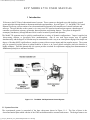
1 Introduction
Welcome
to the ECP line of educational control systems. These systems are designed to provide insight to control
system
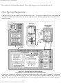
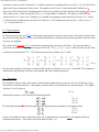
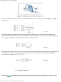
principles through hands-on demonstration and experimentation. Seen in Figure 1.1-1, the Model 750 Control
Moment Gyroscope system consists of an electromechanical plant and a full
complement of control hardware and
software. The user interface to the system is via a easy to use PC based
environment that supports a broad range of
controller specification, trajectory
generation, data acquisition, and plotting features. The system is designed to
accompany introductory through advanced
level courses in control systems and dynamics.
The
Model 750 apparatus may be quickly transformed into a variety of dynamic
configurations. Torque is applied via
direct-acting, reaction, or gyroscopic drive mechanizations. One or two such input torques may be applied
simultaneously and the degrees of freedom may be constrained in such a way as
to create plants ranging from simple one
degree of freedom (DOF) rigid bodies
to complex systems with two torque inputs and four angular outputs. The system
may be operated in regions where
its salient behavior is linear, or in a more global workspace where the
behavior is
highly nonlinear. Thus this
dynamically rich system provides a testbed for experiments ranging from
demonstration of
fundamental principles to advanced research.
Figure 1.1-1. The Model 750
Experimental Control System
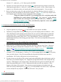
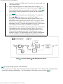
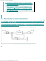
1.1 System Overview
The
experimental system is comprised of the three subsystems shown in Figure
1.1-1. The first of these is the
electromechanical plant which consists of the CMG mechanism and its actuators
and sensors. The design features two
gyroscope_Model750_User_Manual.htm[9/28/2015 2:33:52 PM]
Control Moment Gyroscope - ECP Model750
high torque density (rare earth magnet type) DC servo motors for control effort
transmission, high resolution encoders
for gimbal angle feedback, and low
friction slip rings for signal and motor power transmission across all
gimbals. It also
includes inertial
switches for high gimbal speed detection and safety shutdown and
electromechanical brakes to facilitate
changing dynamic degrees of freedom as
well as securing the system during safety shutdown. The
next subsystem is the real-time controller unit which contains the digital
signal processor (DSP) based real-time
controller, servo/actuator interfaces,
servo amplifiers, and auxiliary power supplies. The DSP – based on the M56000
processor family - is capable of
executing control laws at high sampling rates allowing the implementation to be
modeled as being in continuous or discrete time. The controller also interprets trajectory commands and supports
such
functions as data acquisition, trajectory generation, and system health
and safety checks. A logic gate array
performs
encoder pulse decoding. Two
optional auxiliary digital-to-analog converters (DAC's) provide for real-time
analog signal
measurement. This
controller is representative of modern industrial control implementation. The
third subsystem is the Executive program which runs on a PC under the Windows™ operating
system. This menudriven program is the
user's interface to the system and supports controller specification,
trajectory definition, data
acquisition, plotting, system execution commands,
and more. Controllers are specified via
an intuitive “C-like”
language that supports easy generation of basic or highly
complex algorithms. A built-in
auto-compiler provides for
efficient downloading and implementation of the
real-time code by the DSP while remaining within the Executive. The
interface supports a wide assortment of
features that provide a friendly yet powerful experimental environment.
1.2 Manual
Overview
The
next chapter, Chapter 2, describes the system, including the Executive program,
and gives instructions for its
operation . Section 2.3 contains important information regarding safety and is
mandatory reading for all users prior to
operating this equipment. Chapter 3 is a self-guided demonstration in
which the user is quickly walked through the
salient system operations before
reading all of the details in Chapter 2. A description of the system's real-time control
implementation as well
as a discussion of generic implementation issues is given in Chapter 4. Chapter 5 presents
dynamic equations useful
for control modeling. Chapter 6 gives
detailed experiments including system identification
and a study of important
implementation issues and practical control approaches.
2 System Description & Operating Instructions
This chapter contains descriptions and operating instructions
for the executive software and the mechanism. The safety
instructions given in Section 2.3 must be read and
understood by any user prior to operating this equipment.
2.1 ECP
Executive Software
The
ECP Executive program is the user's interface to the system. It is a menu driven / window environment
that the user
will find is intuitively familiar and quickly learned - see
Figure 2.1-1. This software runs on an
IBM PC or compatible
computer and communicates with ECP's digital signal
processor (DSP) based real-time controller. Its primary functions
are supporting the downloading of various control
algorithm parameters (gains), specifying command trajectories,
selecting data
to be acquired, and specifying how data should be plotted. In addition, various utility functions
ranging
from saving the current configuration of the Executive to specifying
analog outputs on the optional auxiliary DAC's are
included as menu items.
2.1.1 The
ECPMV Executive For Windows 95™, 98, & NT
gyroscope_Model750_User_Manual.htm[9/28/2015 2:33:52 PM]
Control Moment Gyroscope - ECP Model750
2.1.1.1 PC System Requirements
The 32-bit ECPMV
Executive code runs best with a Pentium based PC having at least 16 megabytes
of memory. The
hard drive memory usage is less than 12 Megabytes.
2.1.1.2 Installation Procedure
Enter Windows operating system, insert diskette 1 of 4 in the
floppy drive of your computer and “Run” SETUP.EXE.
Follow the installation
dialog boxes. We strongly recommend that you do not modify the default setup
of the directory
structure used by the installation program.
gyroscope_Model750_User_Manual.htm[9/28/2015 2:33:52 PM]
Control Moment Gyroscope - ECP Model750
2.1.3 Background Screen
The Background Screen
, shown in Figure 2.1.-1, remains in the background during system operation
including times
when other menus and dialog boxes are active. It contains the main menu and a display of
real-time data, system status,
and an Abort
Control button to immediately discontinue control effort in the case of an
emergency.
gyroscope_Model750_User_Manual.htm[9/28/2015 2:33:52 PM]
Control Moment Gyroscope - ECP Model750
Figure
2.1-1. The Background Screen
2.1.3.1 Real-Time Data Display
In
the Data Display fields, the
instantaneous commanded position, the encoder positions, the velocity of the
rotor are
shown. The units of the
displayed data may be changed as described in
2.1.3.2 System Status Display
The Control Loop Status
indicates Closed when a *.ALG
file (an algorithm file) is compiled and downloaded to the DSP
board. When it indicates Open, the control loop is not active.
The Motor Status
fields indicate OK unless the current
limits of the respective motor amplifier is exceeded or over-speed
or
over-travel (Axis #2) condition has been detected. If any of these conditions occur, the affected field will
indicate
Limit Exceeded. To clear the current limit condition either
the DSP board must be Reset via the Utility
menu or a control
algorithm must be re-implemented which does not cause a limit
to be exceeded.
The Servo Time Limit field will
indicate OK unless the currently
implemented *.ALG
file is too long and/or complex for the
chosen sampling period. In such case the Limit Exceeded condition will occur and the loop will be
automatically
opened. The user may then either increase the sampling period or
edit the algorithm code to reduce the execution time.
In general the
combination of high sampling frequency, complex control laws and sine sweep
trajectories (these require
more intensive real-time processing than the other
trajectories) may cause the Limit
Exceeded condition displayed on the
Servo Time Limit indicator
2.1.3.3 Abort Control Button
gyroscope_Model750_User_Manual.htm[9/28/2015 2:33:52 PM]
Control Moment Gyroscope - ECP Model750
Also included on the Background Screen is the Abort
Control button. Clicking the mouse on this button simply
opens the
control loop. This is a very
useful feature in various situations including one in which a marginally stable
or a noisy
closed loop system is detected by the user and he/she wishes to
discontinue control action immediately. Note also that
control action may always be discontinued immediately
by pressing the red "OFF" button on the control box. The latter
method should be used in case of
an emergency.
2.1.3.4 Main Menu
Options
The Main menu is
displayed at the top of the screen and has the following choices:
File
Setup
Command
Data
Plotting
Utility
2.1.4 File
Menu
The File menu contains the following
pull-down options:
Load Settings
Save Settings
About
Exit
2.1.4.1 The Load
Settings dialog box allows the user to load a previously saved
configuration file into the Executive. Such file contains all user-specifiable data except for the control
algorithm itself. A configuration file
is any file with a
".cfg"
extension which has been previously saved by the user using Save Settings. Any "*.cfg" file can
be loaded at
any time. The latest
loaded "*.cfg" file will
overwrite the previous configuration settings in the ECP Executive but
will not effect the existing controller residing in the DSP
real-time control. Any changes to the
algorithm will not take
place until the new controller is
"implemented" – see Section 2.1.5.1. The configuration files include information on the
last used control
algorithm file, trajectories, data gathering, and plotting items previously saved. To load a "*.cfg"
file
simply select the Load Settings command and when the dialog box opens,
select the appropriate file from the
directory.[1] Note that every time the Executive program
is entered, a particular configuration file called
"default.cfg" (which the user may
customize - see below) is loaded. This
file must exist in the same directory as
the Executive Program in order for it
to be automatically loaded.
2.1.4.2 The Save
Settings option allows the user to save the current user-specifiable
parameters for future retrieval via
the Load Settings
option. To save a "*.cfg" file, select the Save
Settings option and save under an appropriately named
file (e.g. "pid1dsk.cfg"). By saving the configuration under a file
named "default.cfg" the user
creates a
default configuration file which will be automatically loaded on
reentry into the Executive program. You
may tailor
"default.cfg" to
best fit your usage.
2.1.4.3 Selecting About
brings up a dialog box with the current version number of the Executive
program.
2.1.4.4 The Exit option immediately terminates the
Executive program.
gyroscope_Model750_User_Manual.htm[9/28/2015 2:33:52 PM]
Control Moment Gyroscope - ECP Model750
2.1.5 Setup
Menu
The Setup menu contains the
following pull-down options:
Control Algorithm
User Units
Communications
2.1.5.1 Setup Control Algorithm
allows the user to write control algorithms, compile them, and implement them
via the
DSP based controller. Figure
2.1-2 shows the control algorithm dialog box. The Sampling Period field
allows the user
to change the servo period "Ts"
in multiples of 0.000884 seconds (e.g. 0.000884, 0.001768 etc.). The minimum
sampling period is 0.000884 seconds (1.1 KHz). Note that if the user servo
algorithm is long and/or complex the code
execution may run longer than the
sampling period. In such a case a Servo
Time Limit Exceeded condition will occur
which will cause the control loop to be automatically opened
by the Real-time Controller. The user
may then either
increase the sampling
time or edit the user servo algorithm to reduce
execution time. In general, the
combination of
high sampling frequency, complex control laws and sinusoidal or
sine sweep trajectories (which also require significant
real-time processing)
may cause the Servo Time Limit Exceeded
condition.
Figure
2.1-2. Setup Control Algorithm Dialog
Box
The
User
Code view box displays the
latest user servo algorithm edited or loaded from the disk. You cannot edit
the
algorithm via the view box. You may however browse it via the arrow
keys.
gyroscope_Model750_User_Manual.htm[9/28/2015 2:33:52 PM]
Control Moment Gyroscope - ECP Model750
opens up the ECPUSR Editor where servo algorithms may be
created by the user. Algorithms may also be
created using any text editor if
saved with a “.ALG”
extension. The ECPUSR editor's features
are described below.
Edit
Algorithm
Implement
Algorithm
downloads the user's code from the Editor buffer to the
Real-time Controller. allows the user to bring into the Editor previously saved user
written algorithms saved as *.ALG
files. The
existing algorithm in the Editor will be automatically overwritten.
Load
from Disk
Once
Edit
Algorithm is invoked, the Editor Screen (see Figure 2.1-3) is displayed.
The user may then enter the servo
algorithm text according to the structural
format described in the next section. Under the File menu within
the Editor
Screen, the following options are available:
New
Load
Save
Save as ...
Save changes and quit
Cancel all
Figure 2.1-3. Control Algorithm Editor Window
The New option enables the user to edit a
completely new control algorithm text.
Load
allows
the user to bring into the Editor previously saved user written
algorithms save as *.ALG files. The
existing
algorithm in the Editor will be removed.
Save
as...
provides the user with the ability to save the Editor's content
with a new or different name on the disk.
Save
changes and quit
Cancel
all
saves the changes made in the latest editing session
and returns to the Control Algorithm dialog box.
returns to the Control Algorithm dialog box without
updating the previous version of the user code with the
gyroscope_Model750_User_Manual.htm[9/28/2015 2:33:52 PM]
Control Moment Gyroscope - ECP Model750
changes made in the
latest editing session.
NOTE: The Editor is not case
sensitive. I.e. "kp" or "Kp" or "KP" will be treated as the same
variable.
2.1.5.2 Structure
of User Written Control Algorithm
Any user
written control algorithm code is made up of three distinct sections:
• the definition segment
• the variable initialization
segment
• the servo loop or real-time
execution segment
When the
ECPUSR program down loads the algorithm to the Real-time Controller, it uses
the definition segment to
assign internal q-variables (q1..q100)
to the user variables defined in the definition segment. The variable
initialization
segment is to be used to assign values to the servo gains and/or
coefficients that either remain constant or must be
assigned some initial value
prior to running the servo loop code. The servo loop code segment starts with a
"begin"
statement and ends with an "end" statement. All the legitimate assignment and
condition statements between these two
statements will be executed every Sample
Period provided that the execution time of the code does not exceed the Sample
Period. (If this occurs the " Servo Time Limit Exceeded " condition
will be shown on the background screen and the loop
will be opened up. The user
may then reduce the complexity of the algorithm between the "begin" and the "end"
statements. Alternatively, if appropriate, the Sample Period
may be increased.)
2.1.5.2.1 Definition
Segment
The are 100 general variables q1 to q100
which may be used by the user for gains, controller coefficients, and
controller
variables. These variables are used internally by the Real-time
Controller. They are stored and manipulated as 48-bit
floating point numbers.
For users' convenience, the #define statement may
be used to assign to the q-variables text
labels
appropriate for particular servo algorithms. For example:
#define gain_1 q2 ;assigns to the
variable q2 the name gain_1
or
#define past_pos1 q6 ;assigns
to the variable q6 the name past_pos1
Note that all
the text beyond the comment delimiter ";"
are ignored by the Real-time Controller and may be used for
annotation by the
user. Also the special variables q10, q11, q12 and q13 may be acquired
via the Data menu
along
with other standard collectable data. This feature allows the users
to inspect critical internal variables of their specific
control algorithms in
addition to the command and sensor feedback positions and control effort(s).
In
addition to the 100 general variables, the are eight global variables as follows:
cmd1_pos
cmd2_pos
enc1_pos
enc2_pos
enc3_pos
enc4_pos
control_effort1
control_effort2
gyroscope_Model750_User_Manual.htm[9/28/2015 2:33:52 PM]
Control Moment Gyroscope - ECP Model750
The
first six of these are predefined to contain the instantaneous commanded
positions and actual encoder positions 1 to
4 respectively. The value assigned
to the control_effort global variables by the user
algorithm will be used as the
control effort (i.e. outputs to the DAC’s à
servo amplifiers à
motors) for that particular servo cycle - see example
below.
Important
Note: The above global variable
names must not be used as general variable names by users in any
definition
statement.
2.1.5.2.2 Initialization
Code Segment
In this
segment the user may predefine the algorithm constants (gains and controller
coefficients) and initial values of the
algorithm's variables. For example:
gain_1=0.78 ;assigns to gain_1 the value of 0.78
gain_1=0.78*3/gain_3 ;requires gain_3 to be previously defined
past_pos1=0.0 ; initialize the past position cell
Note that the
above three examples assume that the #define statement was
used in the Definition Code segment to relate
one general variable qi (i=1...100) to the text variables such as gain_1. Also, all
initialization and constant variable
assignments should be done outside the
servo loop code segment to maximize the servo loop execution speed.
Important Note: If the subsequent user specified
servo loop algorithm controls rotor speed (i.e. control_effort1
is an
output) and the rotor speed has been initialized (see Initialize
Rotor Speed, Section 2.1.6.4), the initialization code
must include the
statement “m136=0”. (Alternatively, the Definition Segment could state “#define
rotorspeedreg m136”, and subsequently the initialization code would
state rotorspeedreg=0.) This disables
the background routine that controls the rotor
under Initialize Rotor Speed. If this routine is not disabled, it will
take precedence over the
user’s servo loop routine and the rotor speed will remain constant. This
becomes an issue in routines such as MIMO controllers where some initial
momentum bias is required to for
gyroscopic torque to be effective, but motor
speed control is required to provide reactive torque. The user may
wish to Initialize Rotor Speed,
then take over control of the rotor torque with his/her algorithm.
2.1.5.2.3 Servo
Loop Segment
This segment
starts with a "begin" statement
and terminates with an "end" statement.
All the legitimate assignment and
condition statements between these two
statements will be executed every Sample
Period provided that the execution of
the code does not exceed the Sample Period.
An
Example
Consider the
following user-written control algorithm program:
;***********
Definition code segment***************
#define kpf q1 ;define kpf as general variable q1
#define k1 q2 ;define k1 as general variable q2 and so on
#define k2 q3
#define k3 q4
#define k4 q5
#define past_pos1 q6
#define past_pos2 q7
#define dead_band q8
;**********
Initialization code segment ************
past_pos1=0 ;initialize algorithm variables
past_pos2=0
kpf=0.93 ;initialize constant gains etc.
k1=0.78
k2=3.14
gyroscope_Model750_User_Manual.htm[9/28/2015 2:33:52 PM]
Control Moment Gyroscope - ECP Model750
k3=0.156
k4=7.58
dead_band=100 ;the size of dead band is set at 100 counts
;********** Servo
Loop Code Segment *****************
begin
if ((abs(enc1_pos) !> dead_band)
k1=k1+0.5
else
k1=0.78
endif
control_effort=kpf*cmd_pos-k1*enc1_pos-k3*enc2_pos-k3*(enc1_pos- past_pos1)-k4*(enc2_pospast_pos2)
past_pos1=enc1_pos
past_pos2=enc2_pos
end
This
is a simple state feedback algorithm with a conditional gain change based on
the size of Encoder 1 position. First the
required general variables are
defined. Next, their values are initialized. And finally between the "begin" and the "end"
statement the servo loop code is written which is intended to run every Sample Period. In addition, the "if" and the
"else" statements
are used to change the value of the k1 gain according to the absolute ("abs")
value of Encoder 1
instantaneous position.
2.1.5.3 Language Syntax For Real-time Algorithms
2.1.5.3.1 Constants
Constants
are numerical values not subject to change. They are treated internally as
48-bit floating point numbers (32-bit
mantissa, 12-bit exponent) by the
Real-time Controller. They must be entered in decimal format as the following
examples suggest:
1234
3
03 ;(leading
zero OK)
-27.656
0.001
.001 ;(leading
zero not required)
2.1.5.3.2 Variables
There
are 100 general variables q1 to q100 which may be used by the user for gains, controller
coefficients, controllers
variables and program flow flags. Examples:
q1=10.05 ;(assign to the
variable q1 the values of 10.05)
q2=q1*0.05 ;(assign to the variable q2 the value of q1*0.05)
Note
that when the define statement is used in the Definition Code segment to give
names to the appropriate q variable
then the above to examples may be written
as:
#define gain_1 q1
#define gain_2 q2
.
.
.
gain_1=10.05
gain_2=gain_1*0.05
2.1.5.3.3 Arithmetic
Operators
gyroscope_Model750_User_Manual.htm[9/28/2015 2:33:52 PM]
Control Moment Gyroscope - ECP Model750
The
four standard arithmetic operators are: +,-,*,/. The standard
algebraic precedence rules apply: multiply and divide
are executed before add
and subtract, operations of equal precedence are executed from left to right,
and operations
inside parentheses are executed first.
There
is an additional "%" modulo
operator, which produces the resulting remainder when the value in front of the
operator is divided by the value after the operator. This operator is
particularly useful for dealing with roll over condition
of command or actual
positions.
2.1.5.3.4 Functions
Functions
perform mathematical operations on constants or expressions to yield new
values. The general format is:
{function name} ({expression})
The
available functions are SIN, COS, TAN, ASIN, ACOS, ATAN,
SQRT, LN, EXP, ABS, and INT.
Note: All
trigonometric functions are evaluated in units of radians (not degrees).
SIN
This is the standard trigonometric sine function
sin ({expression})
Syntax
Domain
All real numbers
Domain Units
radians
Range
-1.0 to 1.0
Range units
none
Possible Errors
N/A
COS
This is the standard trigonometric cosine function
cos({expression})
Syntax
Domain
All real numbers
Domain Units
radians
Range
-1.0 to 1.0
Range units
none
Possible Errors
N/A
TAN
This is the standard trigonometric tangent function
tan ({expression})
Syntax
Domain
All real numbers except +/- pi/2, 3pi/2, ...
Domain Units
radians
Range
-1.0 to 1.0
Range units
none
Possible Errors
divide by zero on illegal domain. (may return max. value.
ASIN
This is the inverse sine (arc sine) function with its
range reduce to
+/- pi/2
asin({expression})
Syntax
Domain
-1.0 to 1.0
Domain Units
none
Range
-pi/2 to pi/2
Range units
radians
Possible Errors
illegal domain
ACOS
This is the inverse cosine (arc-cosine) function with its
range
reduced to 0 to pi.
Syntax
acos ({expression})
gyroscope_Model750_User_Manual.htm[9/28/2015 2:33:52 PM]
Control Moment Gyroscope - ECP Model750
Domain
Domain Units
Range
Range units
Possible Errors
atan
Syntax
Domain
Domain Units
Range
Range units
Possible Errors
LN
Syntax
Domain
Domain Units
Range
Range units
Possible Errors
EXP
-1.0 to 1.0
none
0 to pi
radians
illegal domain
This is the inverse tanget function (arc-tangent).
Syntax
Domain
Domain Units
Range
Range units
Possible Errors
SQRT
Syntax
Domain
Domain Units
Range
Range units
Possible Errors
ABS
Syntax
Domain
Domain Units
Range
Range units
Possible Errors
exp ({expression})
atan({expression})
all reals
none
-pi/2 to pi/2
radians
N/A
This is the natural logarithm function (log base e)
ln ({expression})
All positive numbers
none
all real
none
illegal domain
This is the exponentiation function (ex).
Note: to implement the yx function, use exln(y)
instead. A sample
expression would be exp(q1*ln(q2))
to implement q2q1.
All real numbers
none
all positive reals
none
N/A
This is the square root function
sqrt ({expression})
All non-negative real numbers
free
All non-negative real numbers
free
illegal domain
This is the absolute value function
abs({expression})
All real numbers
free
all non-negative reals
free
N/A
INT
This is a truncation function which returns the greatest
integer less
than or equal to the argument, e.g.
(int(2.5) =2 , int(-2.5)=-3)
Syntax
Domain
Domain Units
Range
int({expression})
All real numbers
free
integers
gyroscope_Model750_User_Manual.htm[9/28/2015 2:33:52 PM]
Control Moment Gyroscope - ECP Model750
Range units
Possible Errors
2.1.5.3.5 Expressions
free
none
An
expression is a mathematical construct consisting of constants, variables and
functions. connected by operators.
Expressions can be used to assign a value to
a variable or as a part of condition (see below). A constant may be used as
an
expression, so if the syntax calls for {expression}, a constant
may be used as well as a more complicated
expression. Examples of expressions:
#define variable_1 q1
#define
variable_2 q2
.
.
.
512
variable_1
variable_1
-variable_2
1000*cos(variable_1*variable2)
abs(cmd_pos)
Note
that the define statements should be used to define the user variables in terms
of q variables. In additions, these
variables should have been initialized.
2.1.5.3.6 Variable
Value Assignment Statement
This type of statement calculates
and assigns a value to a variable. Example:
control_effort=
kp*(cmd_pos-enc1_pos)
2.1.5.3.7 Comparators
A comparator
evaluates the relationship between two values (constants or expressions). It is
used to determine the truth
of a condition in Servo Loop Code segment via the --IF statement (see below). The valid comparators are:
= (equal
to)
!= > !> < !< (not
equal to)
(greater
than)
(not
greater than; less than or equal to)
(less
than)
(not less than, greater than or equal to)
Note:
the comparators <= and >= are not valid. The comparators !> and
!< , respectively, should be used in their place.
2.1.5.3.8 Conditional Statement
In the Servo Loop Code segment
between the begin and the end
statements, the if statement may be for conditional
execution of parts of the control algorithm. The format is as follows:
if
( {condition})
valid
expression
gyroscope_Model750_User_Manual.htm[9/28/2015 2:33:52 PM]
Control Moment Gyroscope - ECP Model750
.
.
endif
Also the else statement may be
used as follows:
if
( {condition})
valid
expression
.
.
else
valid
expression
.
.
endif
If the {condition}
is true, with no statement following
on the line of the if statement,
the Real-time Controller will
execute all subsequent statements on the
following lines down to the next endif or else statements.
A {condition} is made up of two
expressions compared via the comparators described above. For Example:
if (control_effort>16000)
control_effort=16000
endif
or,
If
(enc2_pos>1.1*deadband)
kp=1.0
else
kp=1.2
endif
The{condition}
statement
may be in a compound form
using the and and the or
operators as follows:
If
(enc2_pos>1.1*deadband and enc1_pos<enc2_pos)
kp=1.0
else
kp=1.2
endif
Note that the condition in the if statement line must be surrounded
layers of if statements.
by parenthesis. Also
avoid nesting more than three
2.1.5.2 The User
Units dialog box provides various choices of angular or linear units for
several ECP systems. For
Model 750, the
units are fixed. They are “counts” for
the gimbal and rotor angles (encoders 1-4) and for the
commanded positions;
units of rpm for the displayed value of the wheel speed; and units of volts for
the displayed
control effort values. For Model 750, there are 6667 counts per revolution of the rotor (Axis
#1), 24,400 counts per
revolution of Axis #2 (Encoder #2), and 16,000 counts
per revolution for Axes 3 and 4 (Encoders 3 and 4).
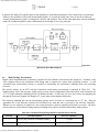
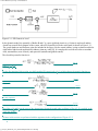
2.1.5.3 The Communications dialog box is usually used only at the
time of installation of the real-time controller. The
choices are serial communication (RS232 mode) or PC-bus mode
– see Figure 2.1-4. If your system was
ordered for
PC-bus mode of communication, you do not usually need to enter this
dialog box unless the default address at 528 on the
ISA bus is conflicting with
your PC hardware. In such a case
consult the factory for changing the appropriate jumpers
on the controller. If your system was ordered for serial
communication (v. direct installation of the DSP board on the
PC bus) the
default baud rate is set at 34800 bits/sec. To change the baud rate consult factory for changing the
appropriate
jumpers on the controller. You may use
the Test
Communication button to check data exchange between the
PC and the
real-time controller. This should be
done after the correct choice of Communication Port has been made. The
Timeout should
be set as follows:
ECP Executive For Windows with Pentium Computer: Timeout ≥ 50,000
gyroscope_Model750_User_Manual.htm[9/28/2015 2:33:52 PM]
Control Moment Gyroscope - ECP Model750
ECP Executive For Windows with 486 Computer: Timeout ≥ 20,000
Figure
2.1-4. The Communications Dialog Box
2.1.6 Command
Menu
The Command menu contains the following pull-down options
Trajectory1 . . .
Trajectory2 . . .
Disturbance . . .
Execute . . .
Initialize Rotor Speed
(or
Disable Rotor Speed Loop)
2.1.6.1 The Trajectory
Configuration dialog boxes
allow the user to specify the shapes of the reference inputs used in
the real
time algorithms. Based on the specified
shapes, the DSP board generates the variables cmd1_pos
and
cmd2_pos that are available to the
user-specified algorithm as real-time control inputs. These dialog boxes, shown in
Figure 2.1.-5, provide a library of
shapes plus the means by which the user may define a custom input. There are two
such boxes, one for each of
the two available system inputs.
Impulse
Step
Ramp
Parabolic
Cubic
Sinusoidal
Sine Sweep
User Defined
A
mathematical description of these is given later in Section 4.1.
gyroscope_Model750_User_Manual.htm[9/28/2015 2:33:52 PM]
Control Moment Gyroscope - ECP Model750
Figure
2.1-5. The Trajectory Configuration
Dialog Box
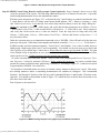
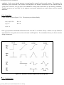
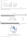
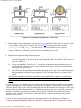
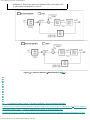
All geometric input
shapes – Impulse through Cubic – may be specified as Unidirectional
or Bi-directional. Examples of
these shape types are shown in
Figure 2.1-6. The bi-directional
option should normally be selected whenever the system
is configured to have a rigid body mode (one that rotates
freely) and the system is operating open loop. This is to avoid
excessive speed or displacement of the system.
Figure
2.1-6. Example Geometric Trajectories
gyroscope_Model750_User_Manual.htm[9/28/2015 2:33:52 PM]
Control Moment Gyroscope - ECP Model750
By selecting the desired shape followed by Setup,
one enters a dialog box for the corresponding trajectory. Examples
of these boxes are shown in Figure
2.1-7. The amplitude is specified in
units consistent with the selected User Units
(Setup
menu). The characteristic durations of
the various shapes are specified in units of milliseconds.
Important
Note: It is possible to specify
amplitudes and/or abruptly changing shapes that exceed the linear range of the
servo amplifiers or cause high angular rates or excessive travel in the
apparatus. These may result in
inaccurate test
results and could lead to a hazardous operating condition or
over-stressing of the apparatus[2]. If in doubt as to whether
the drive linear
range has been exceeded, you may view Control Effort (either by real-time
plotting or via data
acquisition/plotting). Firmware in the real-time controller has routines that will cause the
output to saturate at ± 10 V. These are
transparent to the user. When
specifying an unfamiliar trajectory, the user should generally begin with small
amplitudes, velocities, accelerations, and RMS power levels and gradually
increase them to suitable safe values. Similarly, when specifying control algorithm parameters, one should
begin with conservatively low values; then
gradually increase them. See Section 2.3 on safety.
Figure
2.1-7. Example “Setup Trajectory”
Dialog Boxes
The Impulse dialog box provides for specification of amplitude, impulse
duration, dwell duration, and number of
repetitions.[3] The Step box
supports specification of step amplitude, duration, and number of repetitions
with the dwell
duration being equal to the step duration. The Ramp shape is
specified by the peak amplitude, ramp slope (units of
amplitude per second),
dwell time at amplitude peaks, and number of repetitions. The Parabolic
shape is specified by
the peak amplitude, ramp slope (units of ampl./s),
acceleration time, dwell time at amplitude peaks, and number of
repetitions. In this case, the
acceleration (units of ampl./s2) results from meeting the specified amplitude, slope,
and
acceleration period. The Cubic
shape is specified by the peak amplitude, ramp slope (units of ampl./s),
acceleration
gyroscope_Model750_User_Manual.htm[9/28/2015 2:33:52 PM]
Control Moment Gyroscope - ECP Model750
time, dwell time at amplitude peaks, and number of
repetitions. In this case, the
"jerk" (units of ampl./s3) results from
meeting the specified amplitude, slope,
and acceleration period where the acceleration increases linearly in time until
the specified velocity is reached. Note that the only difference between a parabolic
input and a cubic one is that during the acceleration/deceleration
times, a
constant acceleration is commanded in a parabolic input and a constant jerk is
commanded in the cubic input. Of
course, in a ramp input the commanded acceleration/deceleration is infinite at
the ends of a commanded
displacement stroke and zero at all other times during
the motion. For safety, there is an
apparatus-specific limit
beyond which the Executive program will not accept the
amplitude inputs for each geometric shape.
The Sinusoidal dialog box provides for specification of input amplitude,
frequency and number of repetitions. The Sine Sweep dialog box accepts inputs of amplitude, start and end frequencies
(units of Hz), and sweep duration. Both
linear and logarithmic frequency sweeps are available. The linear sweep frequency increase is
linear in time. For
example a sweep
from 0 Hz to 10 Hz in 10 seconds results in a one Hertz per second frequency
increase. The
logarithmic sweep
increases frequency logarithmically so that the time taken in sweeping from 1
to 2 Hz for example,
is the same as that for 10 to 20 Hz when a single test run
includes these frequencies. There is an
apparatus-specific
amplitude limit beyond which the Executive will not accept
the inputs.
Important Note #1: The logic as to whether to include
the Sine Sweep plotting options is driven by the currently selected
shape under
Trajectory
1. Sine Sweep
must be selected in the Trajectory 1 Configuration
dialog box in order for these
options to be available in Setup
Plot. E.g. if a sine sweep is
desired for Trajectory 2 only,
the user should also select Sine
Sweep for Trajectory
1, and then select Execute
Trajectory 2 Only under Execute – see Section
2.1.6.3. Conversely, if
Trajectory
2 is not to be a sine sweep, then Sine Sweep
should not be selected under Trajectory 1.
Important Note #2: A large open loop amplitude combined
with a low frequency may result in an over-speed condition
in the corresponding
output(s) which will be detected by the real-time controller and the hard-wired
inertia switches
and will cause the system to shut down (see Section 2.3). In closed loop operations, high frequency,
large amplitude
tests may also result in a shut down condition. Any of these conditions will cause the test
to be aborted and the System
Status display in the
Background Screen to indicate Limit Exceeded. To
run the test again you should reduce the input
shape amplitude and then Reset
Controller (Utility menu), and re-Implement a
stabilizing controller (Command menu). In
general, all trajectories that generate
either too high a speed, too large a deflection, or excessive motor power will
cause
this condition – see the safety section 2.3. For a further margin of safety, there is an apparatus-specific
amplitude limit
beyond which the Executive program will not accept the inputs.
The User Defined shape dialog box provides an interface for the specification of
any input shape created by the user. In
order to make use of this feature the user must first create an ASCII text file
with an extension ".trj"
(e.g. "random.trj"). This
file may be accessed from any directory or disk drive using the usual file path
designators in
the filename field or via the Browse
button. If the file exists in the same
directory as the Executive program, then only
the file name should be
entered. The content of this file
should be as follows:
The first line should provide the number of points
specified. The maximum number of
points is 923. This line should
not
contain any other information. The
subsequent lines (up to 923) should contain the consecutive set points. For
example to input twenty points equally
spaced in distance one can create a file called "example.trj' using any text
editor as follows
20
5
10
gyroscope_Model750_User_Manual.htm[9/28/2015 2:33:52 PM]
Control Moment Gyroscope - ECP Model750
15
20
25
30
35
40
45
50
55
60
65
70
75
80
85
90
95
100
The segment time which is a time between each consecutive point can be changed in
the dialog box. For example if a 100
milliseconds segment time is selected, the above trajectory shape would take 2
seconds to complete (100*20 = 2000
ms). The minimum segment time is
restricted to five milliseconds by the real-time controller. When Open Loop is
selected, the units of the trajectory are assumed to be DAC bits (e.g. +16383 =
4.88 V, +16383 = -4.88 V). In Closed
Loop mode, the units are assumed to be the position displacement units
specified under User Units (Setup menu). The
shape may be treated by the system as a
discrete function exactly as specified, or may be smoothed by checking the Treat
Data As Splined box. In the
latter case the shapes are cubic spline fitted between consecutive points by
the real-time
controller. Obviously a
user-defined shape may also cause over-speed of the mechanism if the segment
time is too long
or the distance between the consecutive points is too great.
2.1.6.2 The Disturbance
dialog box is not used in the Model 750 system.
2.1.6.3 The Execute
dialog box (see Figure 2.1-7) is entered after the trajectories are
selected. Here the user commands
the
system to execute the currently specified trajectory(s). The user may select either Normal
or Extended Data Sampling. Normal Data Sampling
acquires data for the duration of the executed trajectory. Extended Data Sampling
acquires data for
an additional 5 seconds beyond the end of the maneuver. Both the Normal and Extended
boxes must be checked to allow
extended data sampling. (For the details of data gathering see
Section 2.1.7.1, Setup Data Acquisition). Either Trajectory
1, or
Trajectory 2, or both may be selected
for execution, and a time delay between them may be specified as shown in
the
figure.
gyroscope_Model750_User_Manual.htm[9/28/2015 2:33:52 PM]
Control Moment Gyroscope - ECP Model750
Figure 2.1-7. The Execute Dialog Box
After selecting the trajectory and data gathering options, the user normally
selects Run. The
real-time controller will
begin execution of the specified trajector(s)). Once finished, and provided the Sample
Data box was checked, the data
will be uploaded from the DSP board into
the Executive (PC memory) for plotting, saving and exporting. At any time
during the execution of the
trajectory or during the uploading of data, the process may be terminated by
clicking on the
Abort button. If the process is aborted before the trajectory has completed, the
associated Commanded Position(s)
(reference input(s)) will be fixed at its current value(s). Finally, if one trajectory has a longer
duration than the other, the
maneuver and data collection will continue until
completion of the longer trajectory.
2.1.6.4 The Initialize
Rotor Speed dialog box is used to specify a spin speed of the rotor in
RPM. After specifying the
desired speed
(between 0 and 800 RPM), and selecting OK,
the real-time controller implements a routine that accelerates
the rotor to the
specified speed and maintains it there. The Command menu will now display the option Disable Rotor
Speed Loop. If this option is
selected, the rotor speed control will be disabled and the rotor will coast to
a stop. Important Note: If the user later implements
a control algorithm that regulates rotor speed (i.e. control_effort1
is an
output) and the rotor speed has been initialized, the initialization code
segment must include the statement m136=0.
(see Setup
Control Algorithm, Initialization Code Segment, Section 2.1.5.2.2) This disables the background
routine that
controls the rotor under Initialize Rotor Speed. If this routine is not disabled, it will take
precedence over
the user’s servo loop routine and the rotor speed will remain
constant. This becomes an issue in routines
such as MIMO controllers where some initial momentum bias is required for
gyroscopic torque to be effective, but motor speed control is required to
provide reactive torque. The user may
wish to Initialize Rotor Speed, then take over control of the
rotor torque with his/her algorithm.
2.1.7 Data
Menu
The Data menu contains the following pull-down
options
Setup Data
Acquisition
Upload Data
Export
Raw Data
gyroscope_Model750_User_Manual.htm[9/28/2015 2:33:52 PM]
Control Moment Gyroscope - ECP Model750
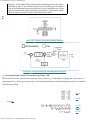
2.1.7.1 Setup
Data Acquisition allows the
user to select one or more of the following data items to be collected at a
chosen multiple of the servo loop closure sampling period while running any of
the trajectories mentioned above – see
Figures 2.1-8 and 4.1-1:
Commanded
Position 1
Commanded
Position 2
Encoder
1 Position
Encoder
2 Position
Encoder
3 Position
Encoder
4 Position
Control
Effort 1 (output
1 to the servo loop or the open
loop command)
Control
Effort 2 (output 2 to the servo loop or the open
loop command)
Variable
Q10[4]
Variable
Q11
Variable Q12
Variable
Q13
Here the user adds or deletes any of the above items by first
selecting the item, then clicking on Add Item or Delete Item. The user must also select the data gather
sampling period in multiples of the servo period. For example, if the sample
time (Ts
in the Setup Control Algorithm) is 0.00442 seconds and you
choose 5 for your gather period here, then the selected
data will be gathered
once every fifth sample or once every 0.0221 seconds. Usually for trajectories with high frequency
content (e.g. Step, or high frequency Sine Sweep), one should choose a low
data gather period (say 10 ms). On the
other
hand, one should avoid gathering more often (or more data types) than
needed since the upload and plotting routines
become slower as the data size
increases. The maximum available data
size (no. variables x no. samples) is 33,586.
2.1.7.2 Selecting Upload
Data allows any previously
gathered data to be uploaded into the Executive. This feature is
useful when one wishes to switch and compare
between plotting previously saved raw data and the currently gathered
data. Remember that the data is automatically
uploaded into the executive whenever a trajectory is executed and data
acquisition is enabled. However, once a
previously saved plot file is reloaded into the Executive, the currently
gathered
data is overwritten. The Upload
Data feature allows the user
to bring the overwritten data back from the real-time
controller into the
Executive.
Figure 2.1-8. The Setup Data
Acquisition Dialog Box
gyroscope_Model750_User_Manual.htm[9/28/2015 2:33:52 PM]
Control Moment Gyroscope - ECP Model750
2.1.7.3 The Export
Raw Data function allows the
user to save the currently acquired data in a text file in a format
suitable
for reviewing, editing, or exporting to other engineering/scientific packages
such as Matlab®.[5] The first line is
a text header labeling the
columns followed by bracketed rows of data items gathered. The user may choose the file
name with a default
extension of ".text" (e.g. lqrstep.txt). The first column in the file is sample
number, the
next is time, and the remaining ones are the acquired variable
values. Any text editor may be used to
view and/or edit
this file. 2.1.8 Plotting Menu
The Plotting menu contains the following pull-down options
Setup Plot
Plot Data
Axis Scaling
Print Plot
Load Plot Data
Save Plot Data
Real Time Plotting
2.1.8.1 The Setup
Plot dialog box (see
Figure 2.1-9) allows up to four
acquired data items to be plotted simultaneously
– two items using the left
vertical axis and two using the right vertical axis units. In addition to the
acquired raw data,
you will see in the box plotting selections of velocity and
acceleration for the position and input variables acquired. These are automatically generated by
numerical differentiation of the data during the plotting process. Simply click
on
the item you wish to add to the left or the right axis and then click on the
Add
to Left Axis or Add to Right Axis buttons. You
must select at least one item for the
left axis before plotting is allowed – e.g. if only one item is plotted, it
must be on the
left axis. You may also
change the plot title from the default one in this dialog box.
Items for comparison should appear on the same axis (e.g.
commanded vs. encoder position) to ensure the same axis
scaling and bias. Items of dissimilar scaling or bias (e.g.
control effort in volts and position in counts) should be placed
on different
axes.
gyroscope_Model750_User_Manual.htm[9/28/2015 2:33:52 PM]
Control Moment Gyroscope - ECP Model750
Figure
2.1-9 The Setup Plot Dialog Box
When the current data (either from the last test run or from
a previously saved and loaded plot file) is from a Sine Sweep
input, several data scaling/transformation options appear in the Setup
Plot box. These include the presentation of data
with
horizontal coordinates of time, linear frequency (i.e. the frequency of the input) or logarithmic frequency. The
vertical axis may be plotted in linear or Db (i.e. 20*log10(data))
scaling. In addition, the Remove
DC Bias option subtracts
the average of the final 50 data points from
the data set of each acquired variable. This generally gives a more
representative view of the frequency
response of the system, particularly when plotting low amplitude data in Db.
Examples of sine sweep (frequency response) data plotted using two of these
options are given later in Figure 3.2-6TBD.
Important Note: The logic as to whether to include the Sine Sweep plotting options is
driven by the currently selected
shape under Trajectory 1. Sine Sweep must be selected
in the Trajectory 1 Configuration dialog box in order for
these
options to be available in Setup Plot. E.g. if a sine sweep is desired for Trajectory
2 only, the user should also
select Sine
Sweep for Trajectory 1,
and then select Execute Trajectory 2 Only
under Execute – see Section 2.1.6.3. Conversely, if
Trajectory
2 is not to be a sine sweep, then Sine Sweep
should not be selected under Trajectory 1.
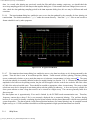
2.1.8.2 Plot
Data generates a plot of the selected items. A typical plot as seen on
screen is shown in Figure 2.1-10.
2.1.8.3 Axis
Scaling provides for scaling or “zooming” of the horizontal and vertical
axes for closer data inspection –
both visually and for printing. This box also provides for selection or
deselection of grid lines and data point labels. When Real-time Plotting is used (see Section 2.1.8.7), the data sweep / refresh speed and
amplitudes may be adjusted via
the Axis Scaling box.
2.1.8.4 The Print
Data option provides for
printing a hard copy of the selected plot on the current PC system
printer. The plots may be resized prior
to printing to achieve the desired print format
2.1.8.5 The
Load
Plot Data dialog box enables the user to bring into the Executive
previously saved ".plt" plot files. Note that such files are not stored in a format suitable for use
by other programs. For this purpose the user should use the
Export
Raw Data option of the Data menu. The ".plt" plot files contain the sampling period
of the previously saved
gyroscope_Model750_User_Manual.htm[9/28/2015 2:33:52 PM]
Control Moment Gyroscope - ECP Model750
data. As a
result, after plotting any previously saved plot files and before running a
trajectory, you should check the
servo loop sampling period Ts
in the Setup Control Algorithm dialog box. If this number has been changed, then
correct it. Also, check the data
gathering sampling period in the Data Acquisition dialog
box, this too may be different and need
correction.
2.1.8.6 The Save
Plot Data dialog box enables the user to save the data gathered by the
controller for later plotting via
Load Plot Data. The default extension is ".plt" under the current directory. Note that ".plt" files are not saved in a
format suitable for use by
other programs. Figure
2.1-10. A Typical Plot Window
2.1.8.7 The Setup
Real Time Plotting dialog box enables the user to view data in real time
as it is being generated by the
system. Thus the data is seen in an oscilloscope-like fashion. Unlike normal (off-line) plotting, real-time
plotting
occurs continuously whether or not a particular maneuver (via Execute,
Command
Menu) is being executed[6]. The setup
for real-time plotting is
essentially identical to that for normal plotting (see Section 2.1.8.1). Because the expected data
amplitude is not
known to the plotting routine, the plot will first appear with the vertical
axes scaled to full scale values
of 1000 of the selected variable units. These should be rescaled to appropriate
values via Axis Scaling. The sweep or data
refresh rate may also be changed via Axis
Scaling when real-time plotting is underway. A slow sweep rate is suitable for
slow system motion or when a
long data record is to be viewed in a single sweep. The converse generally holds for a
fast sweep rate. The data update rate is approximately 50 ms and is limited by
the PC/DSP board communication rate. Therefore,
frequency content above about 5 Hz is not accurately
displayed due to numerical aliasing. The real-time display
however is very useful in visually correlating
physical system motion with the plotted data and is valid for most practical
system frequencies. The data acquired
via the data acquisition hardware (for normal plotting) may be sampled at much
higher rates (up to 1.1 KHz) and hence should be used when quantitative high
speed measurements are desired.
2.1.9 Utility Menu
gyroscope_Model750_User_Manual.htm[9/28/2015 2:33:52 PM]
Control Moment Gyroscope - ECP Model750
The Utility menu contains the
following pull-down options:
Configure Optional auxiliary DACs
Jog Position
Zero Position
Reset Controller
Rephase Motor
Down Load Controller Personality
File
2.1.9.1 The Configure
Auxiliary DACs dialog box (see
Figure 2.1-11) enables the user to select various items for analog
output on
the two optional analog channels in front of the ECP Control Box. Using equipment such as an oscilloscope,
plotter, or spectrum analyzer the user may inspect the following items
continuously in real time:
Commanded Position 1
Commanded Position 1
Encoder 1 Position
Encoder 2 Position
Encoder 3 Position
Encoder 4 Position
Control Effort 1
Control Effort 2
Variable Q10
Variable Q11
Variable Q12
Variable Q13
The scale factor which divides the item can be less
than 1 (one). The DACs analog output is
in the range of +/- 10 volts
corresponding to +32767 to -32768 counts. For example to output the commanded position
for a sine sweep of
amplitude 2000 counts you should choose the scale factor to
be 0.061 (2000/32767=0.061) This gives close to full +/- 10
volt reading on the
analog outputs. In contrast, if the
numerical value of an item is greater than +/- 32767 counts, for
full scale
reading, you must choose a scale factor of greater than one. Note that the above items are always in counts
(not degrees or radians) within the real time controller and since the DAC's
are 16-bit wide, + 32767 counts corresponds
to +9.999 volts, and -32768 counts
corresponds to -10 volts. gyroscope_Model750_User_Manual.htm[9/28/2015 2:33:52 PM]
Control Moment Gyroscope - ECP Model750
Figure
2.1-11. The Configure Auxiliary DACs
Dialog Box
2.1.9.2 The Jog
Position option is not used in the Model 750 system.
2.1.9.3 The Zero
Position option enables the user to reinitialize the current position as
the zero position. Note that if
following errors exists (differences between
the actual positions and the commanded ones), then the actual positions
may be
other than zero even though the commanded position is zero. (Since the action is similar to commanding
an
instantaneous zero valued set point, a sudden small jerk in position may
occur).
2.1.9.4 The Reset
Controller option allows the
user to reset the real-time controller. Upon Power up and after a reset
activity, the loop is closed with
zero gains and there it behaves in the same way as in the open loop state with
zero
control effort. Thus the user should be aware that even
though the Control Loop Status indicates "closed
loop", all of the
gains are zeroed after a Reset. In order to implement (or re implement) a
controller you must go to the Setup Control
Algorithm box.
2.1.9.5 The Rephase Motor option enables a user to simply
rephase a brushless motor's commutation phase angle. This feature is not used by the current Model 750 system
since its motors are internally commutated. 2.1.9.6 The Download
Controller Personality File is
an option which should not be used by most users. In a case where the
real-time controller
irrecoverably malfunctions, and after consulting ECP, a user may download the
personality file if a
".pmc" file exists. In the case of Model 750, this file is named "m750xxx.pmc". This downloading process
takes a
few seconds.
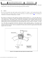
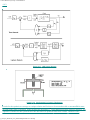
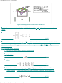
2.2 Electromechanical
Plant
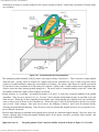
2.2.1 Design Description
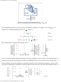
The
plant, shown in Figure 2.2-1, consists of a high inertia brass rotor suspended
in an assembly with four angular
degrees of freedom. The rotor spin torque is provided by a rare earth magnet type DC
motor (motor#1) whose angular
position is measured by a 2000 count per
revolution optical encoder (encoder #1). The motor drives the rotor through a
3.33:1 reduction ratio which amplifies
both the torque and encoder resolution by this factor. The first transverse gimbal
assembly (body
C) is driven by another rare earth motor (motor #2) to effect motion about axis
#2. The motor drives a
6.1:1 capstan to
amplify torque between the adjoining bodies C and B. A 1000 line encoder with 4x interpolation is
gyroscope_Model750_User_Manual.htm[9/28/2015 2:33:52 PM]
Control Moment Gyroscope - ECP Model750
mounted on the motor
to provide feedback of the relative position of bodies C and B with a
resolution of 24,400 counts
per revolution.
Figure 2.2-1. Control Moment Gyroscope Apparatus
The
subsequent gimbal assembly, body B, rotates with respect to body A about axis
3. There is no active torque applied
about this axis. A brake, which is
actuated via a toggle switch on the Controller box, may be used to lock the
relative
position of A and B and hence reduce the system degrees of
freedom. The relative angle between A
and B is measured
by Encoder #3 with a resolution of 16,000 counts per
revolution. Finally, body A rotates
without actively applied torque
relative to the base frame (inertial ground)
along axis 4. The axis 4 brake is
controlled similarly to the axis 3 brake and
the feedback resolution is again
16,000 counts per revolution.
Inertial
switches, or “g-switches” are installed on bodies A, B, and C to sense any
overspeed condition in the gimbal
assemblies. They are set to actuate at 2.1 g’s. For axis 2, limit switches and mechanical stops are provided at the safe
limit of travel. When any of these
normally closed switches sense a high angular rate condition, they open and
thereby
cause a relay to turn off power to the Controller box. When this power is lost, the fail-safe
brakes (power-on-to-release
type) at axes 3 and 4 engage. Also upon loss of power, the windings of
motors 1 and 2 have are shorted, thereby
effecting electromechanical
damping. Thus all axes are actively
slowed and stopped whenever an over-speed or overtravel condition is detected.
Precious
metal sliprings are included at each gimbal axis to provide for continuous
angular motion. These low noise, low
friction, sliprings pass all electrical signals including those of the motors,
encoders, g-switches, limit switches, and
brakes to the Control Box. Important Note #1: The plant
gimbals 2 and 3 must be initially oriented as shown in Figure 2.2-1 in order
gyroscope_Model750_User_Manual.htm[9/28/2015 2:33:52 PM]
Control Moment Gyroscope - ECP Model750
for the dynamic equations of Chapter 5 to be correct. Care must be taken to match the
particular orientation of the
gimbal members (e.g. as seen by the motor orientations) to
achieve correct
polarity. This may be checked via
rotating the respective gimbals in a
positive direction as identified in the
subsequent Figure 5.1-1 and verifying that the
encoder counts are increasing
(for systems purchased as “complete systems, this is
easily seen on the
Executive Program background screen).
Important Note #2: After
releasing Axis 3 and Axis 4 brakes some residual friction may exist. It is
therefore advised to slowly rotate the
corresponding assembly (using a ruler or other
long slender object) several
revolutions to free any excessive friction prior to
performing tests.
2.3 Safety
This
section describes important safety features of the system and cautions
regarding its operation. This
section must be
read and understood by all users and anyone in the physical
vicinity of this equipment prior to operating it. If any
material in this section is not clear to the reader,
contact ECP for clarification before operating the system. This system
can possess high kinetic energy
and therefore it is vital that the safety notices, instructions and warnings of
this section
be followed explicitly.
Important Notice #1: The
system’s safety functions must be verified before each operational
session. When used as instructional
equipment, this means before or at the beginning of each
class in which it is
used. For research, it means as a
minimum, at the beginning of
each day it is used. See instructions 2.3.1 below
Important Notice #2: The
system must be checked visually before each operational session to verify that
the rotor support structure, protective clear rotor cover, brakes, and inertia
switches all appear to be undamaged and securely fastened.
Important Notice #3: In the event of an emergency, control effort should be
immediately discontinued by
pressing the red "OFF" button on front of
the Control Box.
Important Notice #5: Warnings regarding the use of this equipment are provided at
the end of this
section. All persons in
the vicinity of this equipment when the control box is
powered must be aware of
these warnings.
2.3.1 Verifying The System Safety Functions
1. Make sure that that there are no connections to the Control Box
(e.g. DAC inputs or encoder readouts) or that
they are providing no signal
voltages to the box if they are connected.
2. Connect the mechanism to the Control Box and plug the control box
into an appropriate power source.
3. Verify that there is nothing interfering with the free motion of
the gimbals.
4. Turn on power to the Control Box via the red “on” button. With the brakes switched off, verify that
axes 2, 3 and
4 rotate freely.
gyroscope_Model750_User_Manual.htm[9/28/2015 2:33:52 PM]
Control Moment Gyroscope - ECP Model750
5. Manually rotate axis 2 (inner gimbal ring) slowly to one limit of
travel. You should hear a clicking
sound, the
Control Box should power down, and the axis 3 and 4 brakes should
engage. Move assembly off the mechanical
stop and turn the power to the Control Box back on. Move the inner ring in the opposite direction until
contacting
the stop and verify that the Control box powers down and that the brakes
engage. If the system fails
to
automatically shut down after reaching the limit in either direction of travel,
do not further operate the system
and contact ECP before continuing.
6. Manually rotate axis 3 (outer gimbal ring) slowly to get a feel
for how to move it briskly without injuring fingers. Move the gimbal briskly to achieve approximately 100 rpm (1.7
rev/sec). The system should automatically
power down and the axis 3 and axis 4 brakes should engage. If the system fails to automatically shut
down, do
not further operate the system and contact ECP before continuing.
7. Repeat
step 5 for the axis 4 gimbal (vertical yoke at the base of the mechanism). Here it will require
approximately 120 rpm
to cause the automatic shut-down.
2.3.2 Other Safety Features.
Relay
circuits are installed within the Control Box that cause the brakes to engage
and the motors to become shorted
across their windings whenever power is turned
off. The effect of shorting the motor
windings is to cause the motors to
operate in the generating mode and hence to
provide viscous damping. This in turn
decelerates the motion of the
connected assemblies. The
g-switches (inertial switches) that sense the excessive gimbal rates are set to
2.1 g’s. They are normally closed so
that any inadvertent open in the associated circuit will cause the system to
power down and the brakes to engage. The
brakes are of the “fail-safe” power off type meaning that power must
be applied in order for them to be released. Therefore the Control box must be powered and the respective switch
“off” before the associated gimbal is free. Any
inadvertent open in the brake circuit will cause it to engage.
There
are two limit switches and mechanical stops that provide over-travel detection
and protection for Axis 2. When an
over-travel condition is detected, the normally closed switches open and the
controller box is powered off.
The
motor rotor speed is limited by the no-load speed of the spin motor and the
supply voltage. This speed cannot
exceed approximately 1400 rpm. For
equipment purchased as a “Complete System”, the ECP firmware limits the speed
to approximately 825 rpm. For systems
sold as “Plant Only” units, the user must furnish speed detection and control
effort shutdown software to further limit motor speed to 825 RPM maximim.
2.3.3 Safety
Checking Your Controller
While
it should generally be avoided, in some cases it is instructive or necessary to
manually contact the mechanism
when motion control is active. This should always be done with caution and
never in such a way that clothing or hair
may be caught in the apparatus. By staying clear of the mechanism when it is
moving or when a trajectory has been
commanded, the risk of injury is greatly
reduced. Being motionless, however, is
not sufficient to assure the system is
safe to contact. In some cases an unstable controller may
have been implemented but the system may remains
motionless until perturbed – then
it could react violently. In
order to eliminate the risk of injury in such an event, you should always
safety check the controller prior to physically
contacting the system. This is done by lightly grasping a slender,
light object with no sharp edges (e.g. a ruler without
sharp edges or an
unsharpened pencil) and using it to slowly move each gimbal from side to
side. Keep hands clear of
the mechanism
while doing this and apply only light force to each gimbal. If the mechanism does not spin up or
gyroscope_Model750_User_Manual.htm[9/28/2015 2:33:52 PM]
Control Moment Gyroscope - ECP Model750
oscillate then it may be manually contacted – but with caution. This
procedure must be repeated whenever any user
interaction with the system occurs
(either via the ECP Executive program, the user’s data processing hardware or
software or the Controller Box) if the mechanism is to be physically contacted
again.
2.3.4 Start Up and Shut Down Procedures
The
recommended procedure for start up
is as follows:
First : Turn on the PC with the
real-time Controller installed in it.
Second: Turn on the power to Control
Box (press on the black switch).
The
recommended shut down procedure is:
First: Turn off the power to the
Control Box.
Second: Turn off the PC.
FUSES: There are two 3.0A 120V slow
blow fuses within the Control Box. One
of them is housed at the back of the
Control Box next to the power cord
plug. The second one is inside the box
next to the large blue colored capacitor.
2.3.5 Warnings
WARNING #1: Stay clear of and do not touch any part of the mechanism while it is moving, while a trajectory is being
executed, or before the active controller has been safety checked – see Section 2.3.3. WARNING #2: The following apply at all times except when motor drive power is disconnected (consult ECP if
uncertain as to how to disconnect drive power):
a) Stay clear of the mechanism while wearing loose clothing (e.g. ties, scarves and loose sleeves) and when
hair is not kept close to the head.
b) Keep head and face well clear of the mechanism.
WARNING #3: The rotor should never be operated at speeds above 825 RPM. The user must take precautions to assure
that this limitation is not exceeded.
WARNING #4: Never leave the system unattended while the Control Box is powered on.
WARNING #5: Any modification of the Model 750 mechanism or its electronics box could render the system
unsafe. ECP is not responsible for any such modification.
WARNING #6: The power cord must be removed from the Control box prior to the replacement of any fuses.
WARNING #7: In order for the brakes to remain effective after continued use, the associated gimbals must not be moved
repeatedly when the brakes are engaged. The user must minimize forced movement of the gimbals when the brakes are
engaged to minimize their wear.
WARNING #8: In order for the brakes to remain effective, the brake pads and disks must not become contaminated. The
user must assure that no oily or greasy materials are allowed to contaminate the brakes.
3. Start-up & Self-guided
Demonstration
gyroscope_Model750_User_Manual.htm[9/28/2015 2:33:52 PM]
Control Moment Gyroscope - ECP Model750
This
chapter provides an orientation "tour" of the system for the first
time user. In Section 3.1 certain
hardware
verification steps are carried out. In Section 3.2 a self-guided demonstration is provided to quickly orient
the user with
key system operations and Executive program functions. All
users must read and understand Section 2.3, Safety, Before performing any
procedures described in this chapter.
3.1 Hardware
Setup Verification
At
this stage it is assumed that
a) The ECP
Executive program has been successfully installed on the PC's hard disk (see
Section 2.1.2).
b) The actual
printed circuit board (the real-time Controller) has been correctly inserted
into an empty slot of
the PC's extension (ISA) bus.
c) The
supplied 60-pin flat cable is connected between the J11 connector (the 60-pin
connector) of the realtime Controller and the JMACH connector of the Control
Box[7].
d) The other
two supplied cables are connected between the Control Box and the CMG
apparatus;
e) The
mechanism is oriented as shown in Figure 2.2-1. All packing material has been removed and the
mechanism is
constrained only by the brakes on Axes 3 and 4.
f) You
have read the safety Section 2.3. g) You have
verified the system safety functions per Section 2.3.1.
Please
check the cables again for proper connections.
3.1.1 Hardware Verification (For PC-bus
Installation)
Step 1: Switch off power to both the PC and the Control Box.
Step 2: With power still switched off to the Control Box, switch the PC
power on. Enter the ECP program by
double clicking on its icon. You should
see the Background Screen (see Section 2.1.3). Gently rotate the
inner gimbal ring (the one that encloses the brass
rotor). You should see changes in the
Encoder 2 position
and possibly small changes in the Encoder 1 (rotor)
position. The Control Loop Status should indicate "OPEN"
and the Motor 1 Status, Motor
2 Status, and Servo Time Limit should all indicate "OK". If this is the case skip
Step 3 and go to
Step 4.
Step 3: If the ECP program cannot find the
real-time Controller board (a pop-up message will notify you if this is
the
case), try the Communication dialog
box under the Setup menu. Select PC-bus at address 528, and click
on the test button. If the real-time Controller is still not
found, try increasing the time-out in increments of
5000 up to a maximum of
80000. If this doesn't correct the
problem, switch off power to
your PC and then
take its cover off. With the cover removed check again for the proper insertion of the
Controller card. Switch the power on again
and observe the two LED lights on the Controller card. If the green LED comes
on all is well; if
the red LED is illuminated, you should contact ECP for further
instructions. If the green
LED comes
on, turn off power to your PC, replace the cover and turn the power back
on again. Now go
back to the ECP
program and you should see the Encoder 2 position change as you gently rotate
the inner
gimbal ring.
gyroscope_Model750_User_Manual.htm[9/28/2015 2:33:52 PM]
Control Moment Gyroscope - ECP Model750
Step 4: Now connect the power cord to the Control
Box and press the black "ON" button to turn on the power to the
Control Box. You should notice the green power indicator LED lit, but the
motors should remain in a
disabled state. Turn off the Axis 3 and 4 Brakes via the toggle switches on the Control
Box and safety
check the controller
as per Section 2.3.3. Now move Axes 3
and 4. You should see the corresponding
Encoder position values change on the Background Screen of the Executive or via
the user’s own system
interface. Encoder 1 position will usually change as you move axis 3.
This
completes the hardware verification procedure. Please refer again to Section 2.3 for future start up and shut down
procedures.
3.2 Demonstration
of ECP Executive Program
This
section walks the user through the salient functions of the system. By following the instructions below you will
actually implement real-time controllers, maneuver the system through various
trajectories, and acquire and plot data. Note: If at any point in this procedure, the
mechanism or the controller exceed safety limits as detected by the ECP
firmware, the system status display on the Executive Program’s background
screen will indicate Limit Exceeded
in one
or more fields. You must then select Reset Controller (Utility
menu) and repeat the steps leading up to the Limit
Exceeded condition
Step 1: Loading A Configuration File. With the power to the Control box turned off, enter the ECP Executive
program. You should see the Background Display. Turn on power to the Control Box (press on the black
button). Verify that the system is in the
orientation of Figure 2.2-1 with both brakes turned on. If not, turn off
both brakes (toggle
switches on front of the Control Box), re-orient the system and turn on both
brakes. Now
in the Executive program,
enter the File menu, choose Load Setting and
select the file default.cfg. This
configuration file is supplied on the
distribution diskette and should have been copied into the ECP directory
by
now. In fact, it would have been loaded
into the Executive automatically (see Section 2.1.4.1) upon
startup. This particular default.cfg file contains the controller algorithm file name and
other trajectory,
data gathering and plotting parameters specifically saved for
the activities within this section.
Step 2: Implementing A
Controller. Now enter the Setup
menu and choose Control Algorithm. You should see the
sampling time Ts = 0.00884 seconds, and the controller “Gimbal2.alg” loaded. (The file name and its path
should appear in
the “User Code” field of the dialog box.) This controller was designed to close a simple
control loop about
Axis #2 with the other axes stationary. If this algorithm is not loaded you should find it via
“Load
From Disk…“.
Within
the Setup
Control Algorithm dialog box, select Implement Algorithm. The control law is now downloaded to
the
real-time Controller and is immediately effective. Use a ruler or eraser end of a pencil to lightly perturb the
inner black gimbal ring to verify that the control is in effect (it should
resist the pressure you apply) and that it
is stable. (see Sect. 2.3.3,
"Safety Checking The Controller") If the gimbal moves freely, click on the Implement
Algorithm
button again until you notice the servo loop closed. You may
wish to view the real-time algorithm at this point. It implements a simple PD control law about Axis
2 (“control_effort2” is always
sent to motor #2) according to the real-time algorithm structure given in
Section 2.1.5.2. It receives as its
reference input “cmd1_pos”,
which is one of two signals available for this
purpose. You may view the algorithm by scrolling the
viewer within Setup Control Algorithm (the algorithm
may be viewed
but not edited in this window). In
order to get a closer view you may select Edit Algorithm. This
gyroscope_Model750_User_Manual.htm[9/28/2015 2:33:52 PM]
Control Moment Gyroscope - ECP Model750
brings you inside the editor in which
you will later write real-time routines. If you have entered the editor,
select Cancel in the File menu
to exit (do not select Save Changes and
Quit in case some inadvertent change
has been made that would adversely
affect the routine).
Step 3: Setting Up Data Acquisition. Enter
the Data
menu and select Setup Data Acquisition. In this box make sure that
the following four items are selected:
Commanded Positions 1&2, Encoders 2,3 &4, and Control Efforts 1 &
2. Data
sample period should be 2 which means that data will be collected every
second servo cycle (in this
case every 2*0.00884=0.01768 seconds).
Step 4: Executing
A Step Input Trajectory & Plotting. Enter the Command menu and select Trajectory
1. In this box
select Step
and then Setup. You
should see step size = 1000, dwell time =1000 ms and no. of repetitions = 1. If
not, change the values to correspond to
this parameter set. Exit this box and
go to the Command menu. This
time select Execute
and with Normal Data Sampling and Execute Trajectory 1 Only selected, “Run” the
trajectory. You should have noticed a step move of 1000
counts, a dwell of 1 second and a return step
move[8]. Wait for the data to be uploaded from the
real-time Controller to the Executive program running on
the PC. Now enter the Plotting menu
and choose Setup Plot. Select Encoder 2 and Commanded Position 1
for
plotting on the left axis and Control Effort 2 for the
right axis; then select Plot Data. You
should see a plot
similar to the one shown in Figure 3.2-1. The Control Effort data has been shrunk on the
plot and placed below the
other traces using Axis Scaling (Plotting
menu). Figure
3.2-1 Step Response at Axis 2 (Encoder 2)
Step 5: Frequency
Response. Again enter Trajectory
and select Sine Sweep then Setup. You should see the amplitude =
200 counts, max.
freq.= 10 Hz, min. freq.= 1 Hz, sweep time = 29.5 sec., and Logarithmic Sweep selected. Again, if different, change the values to
correspond this set. Exit this box and
go to the Command menu and
select Execute and with
Normal Data Sampling and Execute Trajectory 1 Only selected, “Run” the trajectory. While running this trajectory, you should
notice sinusoidal motion with increasing frequency for about thirty
seconds. Now enter the Plotting menu and choose Setup Plot. You should see a nearly constant amplitude at
low frequency followed by
a resonance at roughly 4.5 Hz and then attenuation at high frequency. Now enter
the Plotting menu
and choose Setup Plot. This time select only Encoder 2 for
plotting (you may of course also
view
Commanded Position 1 data if you wish). Choose Linear Time and Linear Amplitude scaling for the
horizontal and vertical axes; select Remove
DC Bias; then plot the data. You
should see a plot similar to the
one shown in Figure 3.2-2a. Now return to Setup Plot and select Logarithmic Frequency and Db axis scaling
with Remove DC Bias selected. Plot the data. Now the plots should appear similar to those shown in Figure
3.2-2b.
gyroscope_Model750_User_Manual.htm[9/28/2015 2:33:52 PM]
Control Moment Gyroscope - ECP Model750
a)
Linear Time, Linear Amplitude Scaling
a) Log (w), Db Amplitude Scaling
Figure
3.2-2 Frequency Response at Axis 2
The
linear time / amplitude depiction shows the data in a manner that more directly
represents the physical
motion of the system as witnessed. The Log(w)
/ Db scaling presents the data in a way that gives students a
physical
understanding of the Bode magnitude plots commonly found in the
literature. (The upper limit of the
data curve is the experimental Bode magnitude plot.) The resonance at wr, the low
frequency constant
amplitude and high frequency attenuation of –40 Db/decade
are clearly seen from the data.
Step 6: Demonstration
of Gyroscopic Action & Torque Control. Select Abort Control on
the background screen to
disable the current controller. Turn off Brake #4 via the Control Box (Brake
#3 should remain on). Under the
Command
menu go to Initialize Rotor Speed and verify that 300 RPM is
entered. If not enter this amount.
Select
OK. You should see the rotor spin up to 300 RPM. Once the steady state speed is reached –
visible as Encoder
1 Velocity on the
Background Screen – use a ruler or similar object to apply a light
horizontal pressure at the
upper surface of the inner gimbal ring (i.e. cause a
torque about Axis 2). You should see
the Axis 4 (vertical
axis) precess at
an angular velocity w in response to your applied to torque T according to the gyroscopic cross
product T = wxH where H
is the momentum vector associated with the spinning rotor. Do not apply pressure
long enough for
Axis 2 to travel beyond roughly 45 deg. At 90 deg, the system has a singularity and there will
be no gyroscopic
resistance to your torque input. Now apply a light but abrupt
force at the same location and immediately remove it (attempt to apply a light
impulse). You should see a lightly
damped oscillation in Axes 2 and 4. This mode of oscillation is referred to
as nutation and involves the motion at Axes 2 and 4 being 90 degrees
out of phase with each other. Now use
gyroscope_Model750_User_Manual.htm[9/28/2015 2:33:52 PM]
Control Moment Gyroscope - ECP Model750
the ruler or similar object to apply a light pressure to Encoder #3 and thereby
a torque about Axis #4. Again do
not
cause Axis 2 to move greater than 45 deg. from its initial position. Here you will see the rotor precess
about
Axis #2 – again according to T = wxH. Again apply pressure about Axis 4 to return
Axis 2 to its initial
orientation (see Figure 2.2-1)
Step 7: Motion
Control Using Gyroscopic Torque Actuation. With the system set up as in Step 6 and oriented as per
Figure
2.2-1, enter Setup Control Algorithm and load the controller “Gimbal4.alg”. This algorithm controls
motion about the
vertical axis (Axis 4) by damping nutation and steering the rotor’s momentum
vector using
Motor #2. Verify that Ts = 0.00884 seconds, and select Implement
Algorithm. Use a ruler or
similar object to
lightly perturb Encoder #3 and thereby cause a disturbance
about Axis #4. You should again see
Axis #2
precess, but now the controller is regulating the Axis #4 position such
that is does not change. You should
also
detect no nutation mode. Apply
sufficient pressure to return Axis #2 to its original position. Enter
Setup Trajectory 1 and select Step and then Setup. You should see step size = 1000, dwell time
=1000 ms
and no. of repetitions =
1. If not, enter these values. Exit, go to the Command menu, and select Execute. With
Normal
Data Sampling and Execute Trajectory
1 Only selected, “Run”
the trajectory. You should see
an
abrupt step response of the assembly about Axis #4 and a corresponding
rotation of the inner gimbal about
Axis #2 at the beginning and end of each
step. Now plot Commanded Position
1 and Encoder 4 Position on the
left axis and Encoder
2 Position on the right. You should see a trace similar to that of Figure 3.2-3. Note the
relatively fast rise time (Encoder #4) for such a large
assembly and small motor, and the forward and back
nature of the Encoder #2
trace (it is the first derivative of this value that causes the torque applied
about Axis
#4. The derivative data may
also be plotted as Encoder #2 Velocity.) Figure
3.2-3 Axis 4 Step Response Using Gyroscopic Torque Actuation
Step 8: Tracking
Control. Return to Trajectory
1, verify that Unidirectional
moves is not checked, then select Ramp and
then Setup
to enter the Ramp dialog box. You should see Distance = 8000 counts, Velocity
= 4000 counts/s,
Dwell Time = 1000 ms
and Number of Repetitions = 2. If not, enter these values. Exit this box and go to the
Command
menu. Again select Execute
and with Sample Data checked, run the trajectory. You should have seen
a constant velocity
move of 1/4 turn followed by a 1 second pause then a reverse to the –1/4 turn
position, a
pause, then return to the starting point.
Now plot Commanded
Position 1 and Encoder 4 Position on the left
axis and Encoder 2 Velocity on the right. You
should see data similar to that of
Figure 3.2-4. Note the relatively close
tracking of the reference input. The
Encoder 2 velocity acts as the control effort signal according to T = wxH. Its sign is opposite to that of the
acceleration of the assembly (e.g. to that of a conventional control torque acting
on a rigid body) due to the
definition of direction vectors and the cross
product relationship.
gyroscope_Model750_User_Manual.htm[9/28/2015 2:33:52 PM]
Control Moment Gyroscope - ECP Model750
Figure
3.2-4 Axis 4 Ramp Tracking Response Using Gyroscopic Actuation
Step 9: Motion
Control Using Reactive Torque Actuation. With the system oriented as per Figure 2.2-1, turn on
Axis 3 and 4
Brakes. Turn on the “Virtual Brake” for
Axis 2 by clicking on the status button “Axis 2 V-Brake
the background screen[9]. Now perturb the inner gimbal ring with a
ruler or similar object. There
should
be resistance via a tight regulation loop about Motor/encoder #2 to effectively
lock this axis. Enter
Setup
Control Algorithm and load the controller “Gimbal3.alg”. This algorithm controls motion about the
horizontal gimbal ring (Axis 3)
by torqueing the rotor with Motor #1 and causing a reactive torque about Axis
#3. Verify that Ts = 0.00884 seconds, and select Implement
Algorithm. Turn off the Axis 3
brake. Off“
on
Use a ruler or similar object
to lightly perturb the horizontally oriented outer ring and thereby
cause a
disturbance about Axis #3. You
should notice the rotor spin up or down as the system regulates to maintain the
position of Axis 3. Lightly disturb the
outer ring once again to bring the rotor speed back to approximately
zero. If you wish, you may setup Trajectory
2[10]
for a Step of Size
= 400 counts, Dwell Time = 1000 ms
and
Number of Repetitions = 1. To run this trajectory, go to the Command
menu. Select Execute
and with Normal
Data Sampling and Execute Trajectory 2 Only selected, “Run” the trajectory. A plot of the Commanded Position
2
and Encoder
3 Position data is shown in Figure 3.2-5. Turn on the Axis 3 brake and
select Abort Control on the
Background Screen. Note: Never leave
the system
running for extended period
of time in the reaction torque mode. Any disturbances (e.g.slight mass imbalance
of the assembly) can cause
the speed to build up (integrate) over time and lead to an over-speed
condition.
gyroscope_Model750_User_Manual.htm[9/28/2015 2:33:52 PM]
Control Moment Gyroscope - ECP Model750
Figure
3.2-5 Axis 3 Step Response Using Reactive Torque Actuation
Step 10: MIMO
Control Using Reactive and Gyroscopic Control (optional). Steps 1 through 9 above serve to fully
verify the operation of the system. The
following additional step may be of interest to some users. It provides
an interesting demonstration of
two axis simultaneous control.
With the system oriented as
per Figure 2.2-1 verify that the Axis 3 and 4 brakes are turned on and that the
Axis
2 virtual brake is off (the Axis 2 V-Brake status button should indicate
“Off”). Return to Trajectory
1, verify
that Unidirectional
moves is not checked, then select Ramp and then Setup
to enter the Ramp dialog box. Change the amplitude to Distance = 4000 counts, and verify that
the other parameters are as follows: Velocity
= 4000 counts/s, Dwell Time = 1000 ms
and Number of Repetitions = 2. Select OK to exit. Enter Trajectory 2
and verify that Unidirectional moves is also not checked. Enter the setup box for Ramp
and verify that
Distance = 1000
counts, Velocity = 1000 counts/s, Dwell Time = 1000 ms and Number of Repetitions = 3. If
not, enter these values. Under
the Command
menu go to Initialize Rotor Speed and set it to 300 RPM. Select OK and verify that the rotor
spins up
to this speed. Enter Setup
Control Algorithm and load the controller “Gimbals3&4.alg”. Verify that Ts
=
0.00884 seconds, and select Implement Algorithm. Turn off Axis 3 and 4 Brakes. Use a ruler or similar object to
lightly
apply a light torque about Axes 3 and 4 sequentially. You should see the rotor spin up (or down) and
Axis 2 precess as
you did in Steps 7 and 9 above. Do not allow the rotor to spin less than 100
RPM. The gain
of the Gimbal 4 loop
is dependent on rotor speed and therefore excessive Gimbal 2 motion is required
when
wheel speed is too low. If
wheel speed reverses the loop becomes unstable.
Go to
the
Command menu, and select Execute. Select Normal
Data Sampling and Execute Trajectory
2 first,
then Trajectory 1 with delay: and enter 1500 msec. Before
running this maneuver, use a ruler or similar object
perturb the system such
that the inner gimbal ring is vertical (i.e. according to Figure 2.2-1) and the
rotor speed
is approximately 300 RPM. Now select Run .
You
should see controlled motion in a series of constant velocity maneuvers about
Axes 3 and 4. This multiaxis tracking
maneuver makes a stimulating demonstration for students & colleagues! Plot Commanded
Position 1 and Encoder 4
Position of the left axis, and Commanded Position 3 and Encoder 3 Position on
the
right axis. You should see data
similar to that of Figure 3.2-6 which has been scaled to show the motion of one
axis above that of the other.
Turn
off power to the control box.
Figure
3.2-6 MIMO Tracking Response Using Gyroscopic and Reactive Actuation
gyroscope_Model750_User_Manual.htm[9/28/2015 2:33:52 PM]
Control Moment Gyroscope - ECP Model750
This
concludes the Self-Guided Demonstration. Please verify that power to the Control Box is turned off.
4. Real-Time Control Implementation
A
functional overview of the control system is shown in Figure 4.0-1. The system is comprised of three
susbsystems: the
mechanism including motors and sensors, the real-time
controller / drive electronics, and the user/system (“Executive”)
interface
software.
Figure
4.0-1. Overview of Real-time Control
System. This
architecture is consistent with modern industrial control implementation.
A
brief survey of the system architecture is afforded by tracing the data flow as
the system is operated. (An analogous
data flow structure exists in the case where the user’s own controller/data
acquisition hardware and software are
utilized.) The user specifies the control algorithm in the Executive program
and downloads it (via “Implement Algorithm”)
gyroscope_Model750_User_Manual.htm[9/28/2015 2:33:52 PM]
Control Moment Gyroscope - ECP Model750
to the DSP
based real-time controller board. The
DSP immediately executes the algorithm at the specified sample rate. This involves reading the reference input[11]
and feedback sensor (optical encoders) values, computing the algorithm,
and
outputting the digital control effort signal to the digital-to-analog converter
(DAC). In the case of the Model 750
system, there may be two such reference inputs and control effort outputs.
The
DAC converts the resulting stream of digital words to an analog voltage which
is transformed to a current by the
servo amplifier and then to a torque by the
motor. The mechanism transforms the
motor input to motion at the desired
output according to the plant dynamics
(e.g. as approximated by the equations of motion). These plant outputs are
sensed by the encoders, which output a
stream of pulses. The pulses are decoded
by a counter on the DSP board and
made available as a digital position word to
the real-time control algorithm.
When
the user specifies a trajectory and subsequently commands the system to “Execute”
the maneuver, the trajectory
parameters are downloaded to the controller
board. The DSP generates corresponding
reference input values for use by
the real-time control algorithm. Throughout the maneuver, any data specified
by the user is captured and stored in
memory on the board. On completion of the maneuver, the data is
uploaded to PC memory where it is available for
plotting and storage. Details
of these and other salient system functions are given in the remainder of this
chapter.
4.1 Servo
Loop Closure
Servo
loop closure involves computing the control algorithm at the sampling
time. The real-time Controller executes
the
user-specified control law at each sample period Ts. This period can be as short as 0.000884
seconds (approx. 1.1 KHz)
or any multiple of this number. The Executive program's Setup
Control Algorithm dialog box allows the user to alter the
sampling
period. All forms of control laws are
automatically compiled by the Executive program into the M56000
assembly
language prior to downloading to the Controller
("implementing"). The
Controller immediately begins
executing the algorithm. It uses 96-bit real number (48-bit integer
and 48-bit fractional) arithmetic for computation of
the control effort. The control effort is saturated in software
at +/- 32768 to represent +/- 10 volts on the 16-bit DACs
whose range is +/- 10
volts.
4.2 Command Generation
Command generation is the real-time
generation of motion trajectories specified by the user. The parameters of these
trajectories are
downloaded to the real-time Controller through the Executive program via the Trajectory
Configuration
dialog box. This
section describes the trajectories generated in the current control version.
4.2.1 Step Move
Figure 4.2-1a shows a step move demand. The desired trajectory for such a move can
be described by
cp(t) = cp(0)+C for t >0
cv(t)=0 for t >0
cv(0)=¥
Where
cp(t)
and cv(t)
represent commanded position and velocity at time t respectively and C is the
constant step
gyroscope_Model750_User_Manual.htm[9/28/2015 2:33:52 PM]
Control Moment Gyroscope - ECP Model750
amplitude. Such a move
demand generates a strong impulsive torque from the control actuator. The response of a
mechanical system connected
to the actuator would depend on the dynamic characteristics of the controller
and the
system itself. However, in a
step move, the instantaneous velocity and its derivatives are not directly
controllable. Usually step moves are
used only for test purposes; more gentle trajectories are nearly always used
for practical
maneuvers.
4.2.2 Ramp Move
A
ramp demand is seen in Figure 4.2-1b. The trajectory can be
described by
cp(t) = cp(0)+V*t for t >0
cv(t) = V for t >0
ca(0) = ¥
where
ca(0)
represents commanded acceleration at time zero and V is a constant
velocity. Relative to a step demand, a
ramp demand is more gentle, however the acceleration is still impulsive. The commanded velocity is a known constant
during the maneuver.
Figure
4.2-1. Geometric Command Trajectories
Of Increasing Order
4.2.3 Parabolic Move
gyroscope_Model750_User_Manual.htm[9/28/2015 2:33:52 PM]
Control Moment Gyroscope - ECP Model750
Figure
4.2-1c shows a parabolic move demand. Its trajectory can be expressed as:
cp(t) = cp(0)+cv(0)*t+1/2 A*t2 for t >0 <1/2 tf
cv(t) = cv(0)+A*t for t >0 <1/2 tf
ca(t) = A for t >0 <1/2 tf
cj(0) = ¥
where cj(t) represents
commanded jerk at time t and A is a constant acceleration, and tf is the final
destination time. Relative to a ramp
demand, a parabolic demand is more gentle, however the rate of change of
acceleration (jerk) is still
impulsive. Note that the commanded acceleration is a known constant during
the maneuver. The second half of a
parabolic demand uses -A for deceleration.
4.2.4 Cubic Move
Figure 4.2-1d
shows a cubic demand which can be described by
cp(t) = cp(0)+cv(0)*t+1/2 ca(0)*t2+1/6
J*t3 for t
>0 <1/4 tf
cv(t) = cv(0)+ca(0)*t+1/2 J*t2 for t >0 <1/4
tf
ca(t) = ca(0)+J*t for t
>0 <1/4 tf
cj(0) = J
where J
represents a constant jerk. Relative to
all the above demands, a cubic demand is more gentle. The commanded
acceleration is linearly changing during the three
sections of the maneuver. The second
half of a cubic demand uses -J
and the third part uses J again for the jerk
input.
4.2.5 The Blended Move
Any time a
ramp, a parabolic or a cubic trajectory move is demanded the real-time
Controller executes a general blended
move to produce the desired reference
input to the control algorithm. The
move is broken into five segments as shown
in the velocity profile of
Figure 4.2-2. For each section a cubic
(in position) trajectory is planned. Five distinct cubic
equations can describe the forward motion . After the dwell time, the reverse motion can
be described by five more
cubic trajectories. Each cubic has the form:.
cpi(t)= cpi(0)+Vi*t+1/2 Ai*t2+1/6 Ji*t3 i = 1,...,5
Using a known
set of trajectory data (i.e. the requested total travel distance,
acceleration time tacc,
and the maximum
speed vmax, for each
move), the constant coefficients Vi,, Ai, and Ji are determined for each segment of the move by the
real-time Controller. This function is
known as the "motion planning" task. Note that for a parabolic profile Ji=0, and
for a ramp profile Ai is also zero
which further simplifies the task. Having determined the coefficients for each section,
the real-time Controller
uses these values at the servo loop sampling periods to update the commanded
position
(reference input). For example
if the segment is a cubic (J ≠ 0):
ca(k)= ca(k-1) +J*Ts
cv(k)=cv(k-1)+ca(k)*Ts
cp(k)=cp(k-1)+cv(k)*Ts
where Ts is the
sampling period and ca(k), cv(k), cp(k) represent commanded acceleration,
velocity and position at the
kth sampling period.
Figure 4.2-2
Velocity Profile for General Blended Move
4.2.6 Sinusoidal Move
The sinusoidal
move is generated using the following equation:
cp(k)= R* sin (q(k))
where R is the
amplitude, q(k)=w*k*Tp for k=0,1,..., and w is the commanded frequency in
Hz. Tp is set to five
milliseconds
(i.e. k is incremented every 5 ms.). To
further smooth out the trajectory, a cubic spline is fitted between the
points
as follows:
gyroscope_Model750_User_Manual.htm[9/28/2015 2:33:52 PM]
Control Moment Gyroscope - ECP Model750
cp'(k)= (cp(k-1)+4*cp(k)+cp(k+1))/6
For the linear
sine sweep, w(k) = a*Tp, where a
is a constant determined by the difference between the maximum and the
minimum
frequency divided by the sweep time
a
=(wmax - wmin) / sweep
time
For the
logarithmic sweep
w
= wmin *10 (B-A)*(k*Tp)/sweep time
where A and B
are defined according to
A
log10(wmin), B
log10(wmax)
4.3 Brush
Type DC Servo Motor and Drive Amplifier
The control
effort at the kth
sampling period is the input to a 16-bit DAC which provides an analog
signal for the motor
amplifier. The amplifier operates in a transconductance
mode providing a current (as opposed to voltage) demand to the
motor which in
turn represents a torque demand from the motor. To provide the current source capability an analog
proportional
plus integral (PI) controller is implemented within the amplifier for tracking
the demanded current. Referring to the
block diagram of Fig. 4.3-1, the transfer function between the motor current
and the DAC output
(control effort) is given by:
(4.3-1)
Here kc is the DAC
gain in volts/count (10 volts per 32767 counts), kA is the amplifier forward gain
which is
dimensionless (V/V), R is the motor armature and brush resistance in
ohms, L is the motor armature inductance in
henrys, kb is the motor
back emf constant in v/(rad/s), kt is the motor torque constant in Nm/ampere, km is the
mechanical advantage constant which is the ratio of the force generated by the
belt driving the sliding rod to the torque
generated by the motor (N/Nm), and
G(s) is the transfer function between current and the motor velocity. In current
mode drive amplifier, both the
proportional gain kp
and the integral gain ki of the amplifier are chosen to be very high
relative the
inner back emf loop within the practical range of motor operation. As a result,
the effect of the inner loop
may be ignored and the transfer function may be
simplified to:
(4.3-2)
At steady state
this transfer function becomes:
(4.3-3)
The force
delivered to the sliding rod at steady state then becomes:
gyroscope_Model750_User_Manual.htm[9/28/2015 2:33:52 PM]
Control Moment Gyroscope - ECP Model750
(4.3-4)
In general, the
analog PI controller gains of the amplifier are such that the dynamics of the
current loop are much faster
relative to the dynamics of the motor and
mechanical plant. As a result the steady state value of current is achieved
virtually instantaneously relative to changes in velocities and positions. Thus
in this transconductance (current feedback)
mode, the combined amplifier/ motor
combination can be though of as a force generator. Figure 4.3-1. Mechanism Drive Block Diagram
4.4 Multi-Tasking
Environment
Digital
control implementation is intimately coupled with the hardware and software
that supports it. Nowhere is this
more
apparent than in the architecture and timing used to support the various data
processing routines. A well
prioritized
time multi-tasking scheme is essential to maximizing the performance attainable
from the processing
resources. The
priority scheme for the ECP real-time Controller's multi-tasking environment is
tabulated in Table 4.4-1. The
highest
priority task is the trajectory update and servo loop closure computation which
takes place at the maximum rate
of 1.131 KHz (minimum sampling period is
0.000884 seconds). In this case, the
user may reduce the sampling rate
through the Executive Program via changes to
Ts in
the Setup
Control Algorithm dialog
box. The
trajectory planning task has the third highest priority and is serviced at a
maximum rate of 377 Hz. Here the
parameters for a new trajectory need not be calculated every time this task is
serviced by the real-time Controller. Whenever a new trajectory is required (i.e. the current trajectory is
near its completion) this task is executed. The lower
priority tasks are system house keeping routines including
safety checks, interface and auxiliary analog output.
Table
4.4-1 The Multi-Tasking Priority Scheme of the Real-Time Controller
Priority
Task Description
Service Frequency
1
Servo Loop Closure & Command
Update
1.1
KHz
2
Trajectory Planning
377
Hz
gyroscope_Model750_User_Manual.htm[9/28/2015 2:33:52 PM]
Control Moment Gyroscope - ECP Model750
3
Background Tasks including User
Interface,
Auxiliary DAC Update, Limit checks etc.
Background (In time
between other tasks)
The higher
priority tasks always prevail over lower ones in obtaining the computational
power of the DSP. This multitasking
scheme is realized by a real-time clock which generates processor interrupts.
4.5 Sensors
There
are four incremental rotary shaft encoders used in the Model 750. Encoders 1 and 2 are driven directly off the
motor shafts and have an optical resolution of 500 and 1000 lines per
revolution respectively.[12] The remaining two
encoders have a resolution
of 4000 pulses per revolution. The
encoders are an optical type whose principle of operation is depicted in Figure
4.5-1. A low power light source is
used
to generate two 90 degrees out of phase sinusoidal signals on the detectors as
the moving plate rotates with respect
to the stationary plate. These signals are then “squared up” and
amplified in order to generate quadrate logic level
signals suitable for input to
the programmable gate array on the real-time Controller. The gate array uses the A and B
channel
phasing to decode direction and detects the rising and falling edge of each to
generate 4x resolution – see Figure
4.5-2. The pulses are accumulated continuously
within 24-bit counters (hardware registers). The contents of the
counters are read by the DSP once every servo (or
commutation) cycle time and extended to 48-bit word length for high
precision
numerical processing. Thus the
accumulation of encoder pulses provides an angular position measurement
(signal) for the servo routines.
Figure 4.5-1 The Operation Principle of Optical
Incremental Encoders
gyroscope_Model750_User_Manual.htm[9/28/2015 2:33:52 PM]
Control Moment Gyroscope - ECP Model750
Figure 4.5-2. Optical Encoder Output
4.6 Auxiliary Analog Output (System Option)
A
system option provides two analog output channels in the Control Box which are
connected to two 16-bit DACs which
physically reside on the real-time
Controller. Each analog output has the
range of +/- 10 volts (-32768 to +32767
counts) with respect to the analog ground. The outputs on these DACs are updated by the
real-time Controller as a low
priority task. However, for virtually all trajectories (e.g. for sine sweep up to
approx. 25 Hz) the update rate is
sufficiently fast for an oscilloscope or
other analog equipment to inspect the various internal Controller signals. See the
section on the Executive Program's Utility menu for the available signals to output on
these DACs.
5. Plant Dynamic Models
This chapter
develops equations of motion for the four degree of freedom
(DOF) gyroscope. These
equations are
presented in a form suitable to the subsequent controls
design and analysis. Coordinate frame
and dynamic state
conventions are defined to uniquely specify the motion and
configuration of the system. Kinematic
quantities are also
defined as well as the inertiamatrices
of the rigid bodies comprising the system. 5.1.1
Coordinate Frame
Figure 1 shows
the 4 DOF gyroscope comprised of gimbals (A,
B, and C) along with an axi-symmetric disk (D). [13]
gyroscope_Model750_User_Manual.htm[9/28/2015 2:33:52 PM]
Control Moment Gyroscope - ECP Model750
Figure 5.1-1. Coordinate Frame
Definitions
Dextral sets of orthogonal unit
vectors ai, bi, ci, and di
(i=1,2,3) are fixed in A, B,
C, and D, respectively. An
inertial (or
gyroscope_Model750_User_Manual.htm[9/28/2015 2:33:52 PM]
Control Moment Gyroscope - ECP Model750
Newtonian) reference frame is defined as N, in which a dextral set of orthogonal unit vectors Ni (i=1,2,3) are fixed. Four
angles specify the configuration of the
system. The angular travel of D in C
in the direction d2 is
defined as q1,. However as will be shown later, the
displacement of the rotor is typically not used explicitly in the dynamics
and control
study of this system – rather, the speed of D in C, w1, will generally be considered. The angle q2 is defined as the
rotation about c1 of C
relative to B. Similarly, q3 is defined as the angular rotation about b2 of B relative to A. Finally,
q4
is defined as the angular rotation about a3
of A relative to N. The configuration shown in Fig. 1 reflects qi=0 (i=1,
…,4). See also Section 5.1.3
5.1.2 Mass Properties
For this system, the mass centers[14]
of all the bodies comprising the system are at the center of the disk (D) which is also
the center of all the
gimbal axes. Thus, only rotational
dynamics are considered in the following analysis and the effects
of gravity
are neglected.
The central inertia matriciesmatrices
of the bodies comprising the system are given below. Note that each matrix is
given in the coordinate frame attached
to the respective body. The Ix, Jx, Kx
(x = A, B, C, and D) elements
are the scalar
moments of inertia about the ith
(i= 1,2,3) direction respectively in
bodies A, B, C, and D.
(5.1-1)
Note that only moments of inertia
are considered while products of inertia are set to zero. The Model 750 mechanism is
such that this
simplification is valid for most dynamic and control modeling purposes. 5.1.3 Kinematics
The rectilinear velocities of the
mass centers of all the bodies comprising the system are zero since all the
mass centers
are fixed in N (as
discussed above). Only angular
velocities need to be considered in the present analysis. The angular
velocity of A in N is given as
(5.1-2)
Adopting this
notation, we now define the following quantities
(5.1-3)
(5.1-4)
(5.1-5)
The following kinematical
differential equations relate the generalized coordinates to the angular
speeds.
(5.1-6)
(5.1-7)
(5.1-8)
Finally, the
coordinates of any of the body frames may be transformed to the inertialframe
through the following
transformation matrices. These follow from inspection of Figure 5.1-1.
gyroscope_Model750_User_Manual.htm[9/28/2015 2:33:52 PM]
Control Moment Gyroscope - ECP Model750
(5.1-10)
(5.1-11)
(5.1-12)
c2 = d2 (5.1-13)
The simplified
expression of Eq.(5.1-13) results from the axial symmetry of D and by
recognizing that only angular
velocity of the rotor (w1) - not its
position (q1) - is needed
in the dynamics and control study of this system.
5.1.4 System Inputs
Two inputs are
considered for this system. The first
is a torque, T1, applied
to D by C (via the rotor spin motor) which
results in the following torques
on D and C
TD
= T1d2 (5.1-14)
TC
= -T1d2 (5.1-15)
The second input
is a torque, T2, applied to C
by B (via a gimbal motor/capstan drive)
which results in the following
torques on C
and B
TC
= T2c1 (5.1-16)
TB
= -T2c1 (5.1-17)
5.2 Nonlinear Dynamics
Equations
(5.1-1) through (5.1-17) uniquely define the dynamic configuration of the
system. The equations of
motion and may
be solved for via Lagrange’s equations, Kane’s method or other techniques using
symbolic
manipulation programs such as AUTOLEV™, ST/Fast™, AUTOSIM™, or
Mathematica™. The resulting
equations
are given explicitly in Appendix A and are of the form
(5.2-1)
(5.2-2)
(5.2-3)
(5.2-4)
These
equations are not dependent on the angular positions q1 andq4. This is explained by inspection of Figure
5.1-1
where it is seen that the dynamic description of the system would be
identical for any arbitrarily assigned positions of
the rotor and base. Certain of the equations are also
independent of particular angular velocities and accelerations, ,
and . In some cases, the physical interpretation
of the independence is straightforward. Equation (5.2-1) for example
gyroscope_Model750_User_Manual.htm[9/28/2015 2:33:52 PM]
Control Moment Gyroscope - ECP Model750
sums forces acting on the rotor disk in the
spin direction. From Figure 5.1-1 and
the constraints of the system, it is clear
that angular accelerations at the
second gimbal, ,
do not effect rotor velocity.
5.3 Linear Dynamics
5.3.1 Linear Equations About Any
Operating Point
The linearized equations of
motion are found as the first two terms (zeroeth and first order) in the
Taylor’s series
expansion of Equations (5.2-1 through -4) about the operating
point [more explicitly Equations (A.2-3 through -6) are
used in the
derivation]. The operating point (which is a neutrally stable equilibrium point)
is defined as
w1
= W (5.3-1)
q2
= q2o(5.3-2)
q3
= q3o (5.3-3)
Using these definitions, the linearized equations become
T1
- JD 1
- JD cos(q2o) 3
- JD sin(q2o) cos(q3o) 4
= 0 (5.3-4)
T2
+ JD W cos(q2o) cos(q3o) w4 + sin(q3o) (IC
+ ID)
4 - JD W sin(q2o) w3 - (IC
+ ID)
2
=
0 (5.3-5)
1 - sin(q2o) cos(q2o) cos(q3o) (5.3-6)
(JC + JD - ID - KC) 4
- (JB + JC + JD - sin(q2o)2 (JC + JD
- ID
- KC)) 3
= 0
JD W sin(q2o) sin(q3o) w3 + sin(q3o) (IC
+ ID) 2
- JD W cos(q2o) cos(q3o) w2 - JD (5.3-7)
sin(q2o) cos(q3o) 1
- sin(q2o) cos(q2o) cos(q3o) (JC
+ JD - ID - KC) 3
- (ID + KA + KB + KC
+ sin(q2o)2
(JC + JD
- ID
- KC) + sin(q3o)2 (IB + IC
- KB
- KC
- sin(q2o)2 (JC + JD - ID - KC))) 4
= 0
JD W sin(q2o) w2 - JD W sin(q2o) sin(q3o) w4 - JD cos(q2o)
Note that the linear equations do not depend on an operating
point for q4 because they
are valid for any value of q4
chosen as an operating
point. The above equations are
highly useful in that they specify the linear plant dynamics for
any arbitrary
operating point and for all possible configurations of the Model 750 apparatus.
With symbolic manipulation,
these equations may be expressed in state space form as
gyroscope_Model750_User_Manual.htm[9/28/2015 2:33:52 PM]
Control Moment Gyroscope - ECP Model750
(5.3-8)
A Matlab® script is furnished with the Model 750 system that
generates the above plant model for a given set of mass
properties and nominal
states, W,
q2o, and q3o.
5.4 Special Cases
We shall further simplify the dynamics for several special
cases that are studied in the Experiments that follow. In all
such cases the operating point is
about q2o = 0, q3o
= 0, w1 = W. Here
W is the
spin speed of the rotor disk (D). Evaluating at this point, Eq’s (5.3-4
through –7) become
T1
- JD 1
- JD 3
= 0 (5.4-1)
T2
+ JD W w4 - (IC + ID)
JD
1 + (JB
J W w + (I
D
2
D
+ JC + JD)
2
=
3
=
+ KA
+ KB + KC)
0 (5.4-2)
0 (5.4-3)
4
=
0 (5.4-4)
5.4.1 Special Case #1: All Gimbals Free (Reaction & Gyroscopic
Torques Acting)
This
is identically the case given by equations (5.4-1 through –4) and is depicted
in Figure 5.4-1. In the figure, the
unit
vectors c1 and d2
(see Figure 5.1-1) are normal to a3
(i.e. T1 and T2 are directed
horizontally).
Figure 5.4-1. All Gimbals
Free Configuration (q
gyroscope_Model750_User_Manual.htm[9/28/2015 2:33:52 PM]
= 0, q
= 0)
Control Moment Gyroscope - ECP Model750
2o
3o
For the purposes
of controls modeling, equations (5.4-1 through –4) may be expressed in state
space form as
(5.4-5)
The system is seventh order[15]. An eigenvalue solution of the dynamics
matrix will result in one rigid-body mode (two
poles at zero)[16],
three additional poles at the origin representing the kinematic differential
equations, and two complex
poles corresponding to the nutation frequency and
associated oscillatory mode that couples gimbals w2
and w4.
The transfer function q3(s)/T1(s) is
found by solving the Laplace transforms of Eq’s (5.4-1, -3) for q3. Similarly, the
Laplace transforms of Eq’s (5.4-2, -4) are solved to find q4(s)/T2(s) and q2(s)/T2(s). The resulting expressions are:
(5.4-6)
(5.4-7)
(5.4-8)
5.4.2 Special Case #2: Gimbal #3 Locked (Gyroscopic
Torque Only)
In this configuration, gimbal
axis 3 is locked (w3 = 0)
so that bodies A and B become one in the same. The resulting
plant, depicted in Figure
5.4-2, is useful for demonstrations of gyroscopic torque action where the
position and rate, q4
and w4, may be controlled by
rotating gimbal#2 while the rotor is spinning. gyroscope_Model750_User_Manual.htm[9/28/2015 2:33:52 PM]
Control Moment Gyroscope - ECP Model750
Figure
5.4-2. Gimbal #3 Locked, All Others Free (q2o
= 0, q3 = 0)
The
corresponding dynamical expressions may be obtained from equations (5.4-1 through –4) by setting
3=
0 in
equation (5.4-1) and disregarding equation (5.4-3)[17]. These are
T1
- JD
1 =
0 (5.4-9)
T2
+ JD W w4 - (IC + ID) 2
= 0 (5.4-10)
J W w + (I + K + K + 0K )
D
2
D
A
B
C
4
= 0 (5.4-11)
These equations may be expressed in state space form as
(5.4-12)
Here we see that the kinematic
differential equation involving q3
disappears as does one pole of the rigid body mode. A
single pole from the former rigid body pair remains
corresponding to the rotor spin speed as does the nutation mode.
In these equations, the rotor
spin dynamics are decoupled from those of the second and fourth gimbals. Since the rotor
speed may be independently
controlled, the salient dynamics become those involving motion at the gimbal
locations, i.e.
gyroscope_Model750_User_Manual.htm[9/28/2015 2:33:52 PM]
(5.4-13)
Control Moment Gyroscope - ECP Model750
The
realization given by Eq. (5.4-13) is non minimal since it has four state
variables while the transfer functions
q4(s)/T2(s)
and q2(s)/T2(s)
are respectively third and second order. A minimal realization where q4
is a state follows by
eliminating the rows and columns corresponding to q2 in Eq.(5.4-13). A minimal realization where q2 is a state follows
by
integrating Eq.(5.4-11) – assuming initial values of q2 and w4 are zero – and substituting
back into Eq.(5.4-10) from
which the realization follows by inspection. The resulting systems are
(5.4-13a)
(5.4-13b)
The transfer functions q4(s)/T2(s) and q2(s)/T2(s) are
identical to Eq’s (5.4-7, -8) respectively
5.4.3 Special Case #3: Gimbal #3 Locked. Velocity Regulation of w2
In this
configuration, gimbal 3 is again locked and the angular velocity, w2,
at gimbal 2 is an input to the system. In
practice, such a system may be approximated by closing a high authority
control loop about w2, then using w2
as the
input to the system for control of q4. The salient dynamics are given by
Eq.(5.4-11) which may be expressed in state
space and transfer function forms
as
(5.4-14)
(5.4-15)
This
is dynamically equivalent to a rigid body plant with torque input -w2W JD and inertia ID+KA+KB+KC.
5.4.4 Special Case #4: Gimbal #2 Locked (Reaction
Torque on Bodies B&C)
In this
configuration bodies B and C become one in the same. The resulting plant, depicted in Figure
5.4-3, demonstrates
reactive torque where the torque used to change the rotor
speed acts on the combined bodies B
and C and may be used to
control
their position, q3.
gyroscope_Model750_User_Manual.htm[9/28/2015 2:33:52 PM]
Control Moment Gyroscope - ECP Model750
Figure
5.4-3. Gimbal #2 Locked, All Others Free (q2
= 0)
In this case,
the dynamic expressions may be obtained from equations (5.4-1 through –4) by setting
2=
0 and
4=
0. This results in
(5.4-16)
This system possesses the rigid body mode involving the
rotor and gimbal axis 3 and the pole associated with the
kinematic differential
equation for q3. In typical dynamics and control study of
this system, the motion of the gimbal,
q3, is of primary importance and the
relevant system is the second order one
(5.4-17)
The rotor speed is normally only of concern as it relates to
hardware limitations such as maximum safe operational speed
or limitations as
to the spin motor’s torque/speed characteristic. The rotor speed may be found by integrating the
expression in the
middle row of Eq.(5.4-12), i.e.
(5.4-18)
6 . E x p e r i m e n t s
This chapter details experiments
that identify the plant characteristics and parameters; implement a variety of
control
gyroscope_Model750_User_Manual.htm[9/28/2015 2:33:52 PM]
Control Moment Gyroscope - ECP Model750
schemes; and demonstrate many important dynamic and control
principles. The versatility of the
software / hardware
system allows for a much broader range of experimental uses
than will be described here and the user is encouraged to
explore whatever
topics and methodologies may be of interest. The safety portion of this manual, Section 2.3, must be
read and
understood by any user prior to operating this equipment. A graphical
description of the Gyroscope apparatus is shown in Figure 6.1-1. This should be referred to in following the
instructions of this section.
Figure
6.1-1. Control Moment Gyroscope
The instructions
in this chapter begin at a high level of detail so that they may be followed
without a great deal of
familiarity with the apparatus and the Executive
program’s system interface and become more abbreviated in details of
system
operation as the chapter progresses. To
become more familiar with these operations, it is strongly recommended
that the
user read Chapter 2 in its entirety prior to undertaking the operations
described here. Remember here, as
always, it is recommended that the user save data and control configuration
files regularly to avoid undue work loss
should a system fault occur.
6.1 System Identification
gyroscope_Model750_User_Manual.htm[9/28/2015 2:33:52 PM]
Control Moment Gyroscope - ECP Model750
This section
gives a procedure for identifying several of the moments of inertia used in the
equations given in Chapter 5. Further
tests measure and verify the plant input and output gain values necessary for
control modeling. Numerical plant
models are then generated. In the
course of these tests, certain fundamental dynamic properties are demonstrated
that
form a basis for the experiments in the sections that follow.
At this point the user must have read and understood the
Safety Section 2.3 before proceeding. Here and in all operating
sessions, the system safety features must be
verified before proceeding.
6.1.1 Inertia Measurement
In
the following tests, three moments of inertia are measured using the principle
of conservation of angular momentum. The remaining moments of inertia are
provided, but could be measured experimentally using this and other fundamental
principles.[18]
Procedure
Inertia Test #1 (JC)
1. Start the ECP Multivariable
Executive program. Select Abort Control
on the Background Screen to
disable any controller that may be still
running on
the DSP board from a previous user. Turn on power
to the Control Box. Use a ruler or other non-sharp object to nudge the various
elements of the system
to verify that there is no unstable control condition
and that the system is safe to manipulate. In this
and all subsequent
experiments, do not move axes 3 and 4 while their brakes are engaged. This leads
to premature wearout of the
brakes. You should see changes in
the encoder counts on the background
screen (for the axes that are not locked)
as you move the apparatus.
2. Setup the mechanism as shown in Figure
6.1-2a. The Axis 3 and 4 brakes are
turned on and off via
toggle switches on the Control Box. The Axis 2 Virtual Brake is engaged via a
button on the
Executive Program background screen. (This brake is effected via a simple linear control loop
that is
closed in firmware resident on the DSP board and uses Motor #2 and Encoder #2
as the
sensor and actuator.) Select Zero Position (Command menu) to
zero the incremental encoder
values at these gimbal positions.
gyroscope_Model750_User_Manual.htm[9/28/2015 2:33:52 PM]
Control Moment Gyroscope - ECP Model750
Figure
6.1-2. Configurations For Moment of
Inertia Tests
3. Write a simple real-time
algorithm to activate Motor #1 (i.e. put control effort values on the DAC) with
a Control Effort equal to the (Commanded Position)/32.[19] Use the global real-time variables
“control_effort1” and “cmd1_pos” for this
purpose. (The Commanded Position values are
subsequently entered via Setup
Trajectory to provide the input to the system.) Review the algorithm
with your instructor or
laboratory supervisor before proceeding to the next step.
4. Implement this algorithm
using the following steps:
a) Enter Setup Control
Algorithm via the Setup menu. Set the Sample Period to Ts =
0.00442 sec. and
select Edit Algorithm. You are now in the control algorithm
editor. If the editor contains any text
select New under File.
b) Type in your algorithm. Select Save
As… and choose an appropriate name and directory to save
this algorithm
in. Close the editor by either selecting
Save Changes and Quit or simply
clicking
on the upper right hand button.
c) Stay well clear of the apparatus when
initially performing the next step. Select Implement Algorithm
to begin immediate execution of
your algorithm. If all is well, there should be no motion of the
system.
In this and all subsequent
experiments immediately after implementing a controller, you must safetycheck
the system using a ruler or other non-sharp, slender object as per the
instructions of Section
2.3.3.
5. Go to Trajectory 1 Configuration under the Setup menu and deselect Unidirectional Moves (this enables
bi-directional trajectories). Enter Impulse[20] and specify a Amplitude of 16000 counts, a Pulse Width of
1000 ms, a Dwell Time of 0 ms, and 2 repetitions (this prepares the controller board to input a 16000 count
positive-going step followed immediately by a 16000 count negative-going one.) Select OK, successively
and enter Setup Data Acquisition (Setup menu). Specify Sensor 1 Position, Sensor 2 Position, Sensor 3
Position, Sensor 4 Position, Control Effort 1 and Control Effort 2 as data to be acquired with a Sample
Period of 2 servo cycles.
6. Go to Execute (Command menu) and verify that the apparatus is in the configuration of Figure 6.12a. Select Normal Data Sampling and Execute Trajectory 1 Only and then Run. You should see the rotor
gyroscope_Model750_User_Manual.htm[9/28/2015 2:33:52 PM]
Control Moment Gyroscope - ECP Model750
spin up then slow down while the inner assembly (bodies B, C, and D) rotates about Axis 3. Is the motion of
the rotor and that of the inner assembly in the same direction or opposite directions? Select OK once the
data from the maneuver has been uploaded.
7. Go to Setup Plot (Plotting menu), and plot the Encoder 1 Velocity and Encoder 3 Velocity data. You
should see the Encoder 1 velocity increase approximately linearly for one second, then decrease
approximately linearly for the following second. The Encoder #3 velocity should show a corresponding
characteristic. Save your plot (via Save Plot Data, Plotting menu).
Inertia
Test #2 (KA)
8. Setup the mechanism as shown in Figure
6.1-2b. In order to improve the quality
of your result,
the following procedure is recommended in setting the initial
orientation of the yoke v. the base
(i.ei.e. q4). Rotate the yoke relative to the base using a very light touch to find a
location where
there is least friction (some residual friction from the brake
may exist in some locations). Although
typically small, any friction may be detected by giving the yoke a very small
initial
velocity and observing how rapidly it stops. The yoke should be positioned to minimize the travel
in any zone
of friction for motion in a counterclockwise direction. (E.g. positioned just beyond a
zone of
friction when moving in a counterclockwise direction).
9. Go to Trajectory
1 Configuration
under the Setup menu, select Impulse and change the Pulse
Width to
2000 ms.. Leave all other
parameters the same as in Step 5 above.
10. Repeat Step 6 to execute the input to the
system. You should see the rotor spin
and the remaining
assembly rotate about the base (Encoder #4). Note the nature of the motion.
11. Setup and plot Encoder #1 and
Encoder #4 velocity data. Save your
plot.
Inertia
Test #3 (IC)
12. Setup the mechanism as shown in Figure
6.1-2c. Set the yoke position as
described in Step 8.
13. Edit
your algorithm from Step 13 above to output cmd1_pos to control_effort2. (i.e. put Trajectory 1 inputs
on DAC2 to drive Motor 2). Select Save Changes and
Quit to exit the
editor. .
14. Stay clear of the apparatus and select Implement
Algorithm to begin immediate execution of your
algorithm. If all is
well, there should be no motion of the system. Safety check the system.
15. Go to Trajectory 1 Configuration, select Impulse and change the Pulse
Width to 200 ms.. Leave all other
parameters the same as in Step 5 above.
16. Repeat Step 6 to execute the input to the
system. You should see the inner gimbal
ring rotate
relative to the outer ring and the remaining assembly rotate about
the base (Encoder #4). The
inner ring
will likely contact the limit switch at the end of the maneuver causing the
Control Box
to power down. This is
normal. If it occurs before completing
a satisfactory test, simply re-power
the Control Box. It is also possible that the limit switches are contacted during
the initial (first 400
ms) portion of the maneuver. If this occurs, reduce the Pulse
Width duration in Step #15 (to say
150 ms.) and repeat the remainder of the
procedure.
17. Setup and plot Encoder #2 and
Encoder #4 velocity data. Save your
plot.
6.1.2 Control Effort Gain Measurement
In
the following tests, the control effort gain for the two plant inputs is
measured using Newton’s second law (in its
rotational form) and the gyroscopic
cross product. These relationships have
the well-known forms
gyroscope_Model750_User_Manual.htm[9/28/2015 2:33:52 PM]
Control Moment Gyroscope - ECP Model750
(6.1-1)
(6.1-2)
where
in the first expression, T is the
applied torque, J is the moment of
inertia about an axis parallel to T, is the
angular acceleration of J about that axis. In the second expression, H is the momentum of the body, w
is the angular
velocity associated with change of direction of the vector H, and T is the applied torque necessary to change the
direction of H.
Control Effort
Gain Test #1 (kg1)
In this test, we
measure the acceleration of the rotor disk to a known control effort signal in
the positive and
negative directions and measure the resulting accelerations.
From the accelerations and rotor inertia value, the
applied torque
and hence control effort gain may be calculated.
1. Setup
the mechanism in the configuration of Figure 6.1-3a. 2. Edit your algorithm from
Step 13 above to output cmd1_pos
to control_effort1. (i.e. the same as in
Inertia tests 1 and
2). Select Save Changes and Quit to exit the editor. Select Implement Algorithm and
safety
check the system. Figure
6.1-3. Configurations For Control
Effort Gain Tests
3. Go to Trajectory
1 Configuration
and verify that Unidirectional
Moves is not selected. Enter
Impulse
and
specify an Amplitude of 16000 counts, a Pulse Width of 4000 ms, a
Dwell Time of 0 ms, and 2
repetitions.
4. Execute
this input with Normal Data Sampling
and Execute Trajectory 1 Only
selected. You should
see the rotor
spin up then slow down and possibly reverse motion.
5. Plot Encoder #1
velocity and control Effort 1
data. Save your plot.
gyroscope_Model750_User_Manual.htm[9/28/2015 2:33:52 PM]
Control Moment Gyroscope - ECP Model750
Control Effort
Gain Test #2 (kg2)
In this test, we
measure the torque required to allow the momentum vector, H, of the spinning wheel to precess
at
some rate w according to Equation (6.1-2). 6. Setup
the mechanism in the configuration of Figure 6.1-3b. 7. Stay
clear of the mechanism and Initialize Rotor Speed (Command Menu) to 400
RPM. Safety check the system once the
rotor has reached approximately 400 RPM
as seen on the Background Screen.
8. Apply light finger
pressure to the upper edge of the inner ring as shown in Figure 6.1-3b. Note what
happens to the motion of the
assembly about Axis #4 (the vertical axis at the base of the unit)? This is
the fascinating phenomenon of
gyroscopic precession. Now apply light
pressure in the opposite
direction. What
happens to the motion of the assembly? For a given amount of finger pressure does
the motion about Axis #4
remain at constant velocity or does it accelerate?
9. Now apply light
finger pressure to the side of Encoder#3 to rotate the assembly about Axis
#4. What
happens to the inner assembly
with respect to Axis #2? Do not exceed q2=± 60
deg. (If a limit switch
is contacted
due to excessive motion in q2, repeat steps 6-8.) Return the inner ring to the approximate
vertical position (q2=0).
10. This time, have a fellow
student apply light finger pressure to the encoder to cause a small rotation
rate
about Axis #4 while you apply a sufficient force on the inner ring (at the
location used in Step 8) to
keep it approximately vertical (q2=0). How does the force (and hence torque about
Axis #2) required
to keep the ring vertical vary with the angular rate about
Axis #4? You may trade places with the
fellow student so that each experiences the nature of the applied force. Return the inner ring to the
approximate
vertical position (q2=0).
11. In the Setup
Control Algorithm dialog box, change sampling period to Ts=0.00884 s. Verify that the
mechanism is in the configuration of Figure
6.1-3b. Locate and Implement the algorithm
“axis2lock.alg” as furnished with the system. This
simple routine regulates the position of Axis 2 to
keep it at the approximate
current position. We shall measure the
control effort required to do so in the
test that follows. Safety check the controller.
12. Rotate the assembly slowly
about the vertical axis and note the Control
Effort 2 values displayed. Do
not rotate the assembly at a sufficiently high rate to cause Control Effort 2 to exceed ± 5V. What has
changed with regard to resistive torque required to
rotate the assembly about the vertical axis (Axis #4)
as experienced in Step
9? 13. Change the Impulse
amplitude to zero (0) counts and leave all else as specified in Step 3. (This will
allow the system to collect data
during the “Execute” period while
maintaining a zero valued reference
input)
14. Practice the following
procedure: Slowly rotate the assembly
about the vertical axis at a rate to cause
approximately 4-5 V of control
effort; release to let the assembly spin freely; wait for a second or two;
reverse
direction to a achieve –4 to –5 V control effort, then release again. The goal
is to measure the
control effort required at motor #2 during the free spinning
periods
of this maneuver. Once this is
consistently achieved, prepare to Execute the Impulse maneuver from Step 13. Select Run, then
perform this
procedure. 15. Plot the Encoder 4Velocity and Control Effort 2 data. Verify that Control Effort 2 had at least some
values in the range of 4 to 5 V
and –4 to –5 V in the portions of the curve when the assembly was
spinning
freely (the velocity data should
be relatively flat during this period). If not, repeat Step 14. Save
your final plot.
6.1.3 Feedback Sensor (Encoder) Gain Measurement
In
these tests, we measure the sensor gain, i.e. the change in sensor signal
output per unit of physical position change. gyroscope_Model750_User_Manual.htm[9/28/2015 2:33:52 PM]
Control Moment Gyroscope - ECP Model750
For the Model 750 system, the sensors are all optical encoders and with
outputs in counts. 1. Turn on the Control Box and
select Abort Control in the
Background Screen. Turn off the Axis 2
Virtual Brake and the Axis 3 and 4 Brakes. 2. Select a starting position
for Axis 4. You may wish to use a piece
of masking tape or other
nonpermanent item to mark this position as precisely
as possible. Select Zero Position (Command
menu) to zero the incremental encoder values at their current position. Rotate the yoke (Axis 4)
through precisely 1
revolution and record the change in encoder counts using a Table similar to
Table
6.1-1.
3. Repeat Step 2 for Axis 3 and
then for Axis 2. For Axis 2, rotate
Body B through one half revolution
only (i.e. the limit stops restrict the
motion to approximately ± 120 deg.). The gain for Encoder #1 is
provided since the spin rotor is not
accessible. 4. For purposes of
increasing numerical precision, the controller firmware multiplies the encoder
and
commanded position signals internally by 32. This factor does not multiply the background display
nor plotted
data, but does the encoderi_pos
and cmdj_pos (i=1,2,3,4; j=1,2) variables as they are
processed in the real-time
algorithms. Thus you must multiply the
measured encoder gains by 32 in
order for them to be properly scaled. Complete the third column of Table 6.1-1. Table 6.1-1. Encoder Gain Measurements
Gain, kei
Axis Number
(Encoder Number)
Output / Rev.
(counts/rev)
1
6667
1061*32
2
3
4
(counts/rad)
Questions / Exercises:
A. In the tests of Section 6.1.1, there was in
each case a torque applied
between two bodies while
the combined bodies we free to rotate about
some axis. Was the motion of the two bodies in the
same or opposite
directions? Was the
angular velocity of the body with greater apparent
inertia greater or less
than that of the body with lesser apparent inertia?
Use the principal of conservation of angular momentum to
explain your
answer. s. I.e. for a system of two
bodies constrained to move about a
single axis with no externally applied
moment:
J1w1+J2 w2
= C (6.1-3)
Where Ji and wi are the respective inertia and
velocity of body i and C is
a constant. What is the approximate shape of the
velocity curve in the positive
control effort and negative control effort
segments (e.g. constant,
linearly increasing, parabolic, etc.)? What would be the approximate
shapes of the
position and acceleration data? Explain. You may plot
these
other derivative values to check your answer (the acceleration data
will be
somewhat noisy due to the numerical differentiation used in
calculating it).
gyroscope_Model750_User_Manual.htm[9/28/2015 2:33:52 PM]
Control Moment Gyroscope - ECP Model750
B. Table 6.1-2 gives moments of inertia of
bodies A through D. Use the
principle
of conservation of angular momentum and plotted test results
from Section
6.1.1 to complete the table for JC, KA, and IC. In
evaluating Eq.(6.1-3), you should
equate the angular momentum at the
beginning and end of the first (positive
control effort) segment of the
input according to
J1w1o+J2 w2o
= J1w1f+J2 w2f (6.14)
and solve for the unknown inertia. Repeat this for the second (negative
control effort) segment and take the average value of the calculated
inertias. This will reduce the effect
of asymmetric effects such as
bearing friction. (Hints: You will need to use the encoder gain values
obtained
in Section 6.1.3 to obtain the measured angular velocities, and
you may need
to add or subtract them in some cases to obtain the
angular velocity relative
to the inertial frame as per Eq.(6.1-4). For the
IC tests, the data of the curve at
the end of the positive control effort
portion and beginning of the negative
control effort one may be
discontinuous (jagged) due to a slight flexibility
in the drive. You
should extrapolate
the velocity characteristics to find where they
intersect and use this value
in your calculation.)
C. In the rotor acceleration tests of Step 5 of
the control gain measurement
experiment (6.1.2), is the acceleration in the
positive control effort
segment of greater, less, or approximately equal magnitude
to that of the
deceleration in the negative control effort segment? If of different
magnitude, what non-ideal
characteristic is this a result of?
In the gyroscopic torque experiments of
Steps 8, 9 and 10, you applied
torques to the system and observed the
resulting motion. Explain your
observations in terms of Eq. (6.1-2). In Step 12 after implementing a
regulating controller to maintain Axis
2 at an approximately constant
position, how did the assembly respond to your
manually applied
torque? How does
this relate to the control effort required by Motor 2 to
keep Axis 2
stationary?
D. For control design and implementation
purposes, it is necessary to
include the control effort gain in the system
model. For our system, this
gain is
the ratio of torque at a particular actuator to control effort counts
at the
output of the real-time control algorithm. I.e.
Ti = ui kui (i=1,2) ˆ(6.1-5)
where Ti and ui are the
respective torque and control effort associated
with the ith plant input and kui
is the control effort gain. This gain
is
comprised of the following product
kui =
kckaktkp (6.1-6)
where:
kc, the DAC
gain, = 10V / 32,768 DAC counts
gyroscope_Model750_User_Manual.htm[9/28/2015 2:33:52 PM]
Control Moment Gyroscope - ECP Model750
ka,
the Servo Amp gain, ≈ 0.4 (amp/V)
kt,
the Motor Torque constant ≈ 0.05 (#1), (0.1) (#2) (N-m/amp)
kp,
the Drive Pulley ratio = 2 3.33 (#1), 6.1
(#2) (N-m out / N-m in)
In Step 5 of Section 6.1.2, you obtained
the acceleration of a known
inertia under a known control effort. Use Eq’s (6.1-1 & -5) to solve for
a
more precise, measurement based, value of ku1. Use the average value
obtained by
considering the acceleration and deceleration portions of
your plot from Step
5. (Hint: in interpreting test data,
the acceleration
can be most accurately found by taking the change in
velocity and
dividing by the change in time. The acceleration data is typically noisy
and difficult to read with
precision.)
In Step 15 of Section 6.1.2, you
obtained the control effort associated
with an angular rate of change of a
known (i.e. calculable) momentum. Use
Eq’s (6.1-2 & -5) to solve for ku2. Use the average value obtained
by
considering the positive and negative Axis #4 velocity portions of
your plot
from Step 15. Use the flatter
portions of the velocity curve
where the assembly was rotating freely (i.e.
you were not touching it).
Table 6.1-2. Moment of Inertia Data
Body
Inertia Element
2
Value
(kg-m )
A
KA
-
B
IB
0.0119
JB
0.0178
KB
0.0297
IC
-
JC
-
KC
0.0188
ID
0.0148
JD
0.0273
C
D
You have now obtained all parameters necessary to
construct numerical dynamic models of the plant. For
control design and implementation purposes, the sensor and
actuator gains must be accounted for so that
the resulting system is properly
scaled. As an example of the
application of these gains, Eq.(5.4-1) becomes
u1 ku1 -
JD 1c/ke1 -
JD 3c/ke3 = 0 (4.4-1)
Where the wic‘s
(i=1,3) are the respective velocities
in units of encoder counts. In such an
application of
system gains, the resulting equations of motion should always
have consistent units (e.g. SI units) when the
real-time variable units are
applied. gyroscope_Model750_User_Manual.htm[9/28/2015 2:33:52 PM]
Control Moment Gyroscope - ECP Model750
Exercises
E. Use the results of this chapter to generate
numerical plant models for the
“special cases” of Sections 4.1.1 through
4.4-4. Use W =400 RPM. Express your results in both state space
and transfer function forms. For
Special Case #2, include both the fourth order and third order (minimal)
state space realizations.
F. Generate a numerical plant model of the
system linearized about the
operating point for the case where:
w1 = 400 RPM
q2o
=20o
q3o =-20o
Express your result in state space
form. Use the same states as those in
Eq. (5.3-8).
6.2 Gyroscopic Dynamics: Nutation &
Precession
This section
measures the nutation and precession of the gyroscope as a function of wheel
speed. It also demonstrates
the damping
of nutation through rate feedback at Gimbal #2, and finally, gives another way
of interpreting precession in
terms of conservation of angular momentum. All tests in this section are performed with
the apparatus in the
configuration of Figure 6.2-1.
Important Notice: From this point on in the instructions, no
specific reminders to perform the required safety procedures
shall be
given. The user must follow the safety
the Safety guidelines of Section 2.3 at all times when operating this
equipment.
Figure 6.2-1. Configuration For All Tests In This Section
6.2.1
Nutation: Frequency & Mode Shapes
Procedure
1. Setup the mechanism as shown in Figure
6.2-1.
2. Write a simple real-time algorithm to
activate Motor #2 (i.e. put control effort values on the DAC) with
gyroscope_Model750_User_Manual.htm[9/28/2015 2:33:52 PM]
Control Moment Gyroscope - ECP Model750
a Control Effort equal to the (Commanded Position)/32.[22] Use the global real-time variables
“control_effort2” and “cmd1_pos” for this
purpose. 3. Go to Trajectory
1 Configuration. Enter Impulse and
specify an Amplitude of 16000 counts,
a Pulse
Width of 50 ms, a Dwell Time of 4000 ms, and 1 repetitions (this prepares
the controller board to input
a 16000 count positive-going impulse followed
immediately by 4 seconds of zero input during which
data is collected.
4. Setup
Data Acquisition (Setup
menu). Specify Commanded Position 1, Sensor 2 Position, Sensor 4
Position, and Control
Effort 2 as data to be acquired with a
Sample Period of 4 servo cycles.
5. Enter the ECP Multivariable
Executive program. Implement your algorithm from Step 2 above with
sampling
period set to Ts = 0.00442
seconds.
6. Initialize
Rotor Speed to 200 RPM and zero the encoder positions (Utility
menu). Execute the
maneuver
selecting Normal Data Sampling
and Execute Trajectory 1 Only .
7. Plot the Encoder 2 and
Encoder 4 Position data and subsequently the velocity data. Note the frequency
of the oscillations and
the relative amplitude and phase of the Encoder 4 response verses the Encoder 2
response. Save your plots.
8. Disable the rotor speed loop
(Command
menu). You may also want to turn off
the Control Box to more
rapidly decelerate the rotor. Wait for the rotor to stop (if you turned off the Control Box,
turn it back
on at this point). Repeat
Steps 6 and 7 for a rotor speed of 400 RPM.
9. Repeat Step 8 for a rotor
speed of 800 RPM.
6.2.2 Precession
Procedure
10. Repeat Steps 1 through 6 of the Section 6.2.1
except in Step 3 setup the Impulse
trajectory for an
Amplitude of 6000 counts, a Pulse Width of 8000 ms, a
Dwell Time of 0 ms, and 1 repetition (this
prepares the controller board to input a 6000 count constant input for 8 seconds). The first maneuver
should be at 200 RPM and
should result in a initial transient series of attenuating nutation
oscillations
followed by a steady state response. Plot the position data for Encoders 2 and 4 and also their
velocity
data. Save your plots.
11. Repeat Step 10 for the 400
and 800 RPM cases. Note the change in
steady state velocity for Encoder 4
with rotor speed.
6.2.3 Nutation Damping
Procedure
12. Augment your algorithm from Step 1 of Section
6.2.1 to add rate feedback damping at Axis 2. I.e. add
a term u2damp of the form
u2damp = -kv q2 s
where kv is the rate feedback
gain. You may use the backwards
difference transformation to
implement discrete time differentiation according
to
gyroscope_Model750_User_Manual.htm[9/28/2015 2:33:52 PM]
(6.2-8)
Control Moment Gyroscope - ECP Model750
where Ts is the sampling period. Use Ts =0.00884 s. in this experiment.
Have your laboratory supervisor review
and approve your algorithms before proceeding. 13. Set the rotor speed to 400
RPM. Beginning with a value of kv =
0.005 Implement your algorithm with
Ts =0.00884
seconds. 14. Repeat Step 10 except
maintain the rotor speed at 400 RPM rotor speed. Do you see a reduction in the
nutation mode amplitude?
15. Repeat Steps 13 and 14 for
various increasing values of kv. Do not exceed kv=0.10, higher values could
lead to excessive numerical noise and damage to the system! How are the nutation oscillations
affected
by increased rate feedback gain? Save
your plot of a case where the nutation is well
damped.
Exercises
A. From the plotted data of Section 6.2.1,
measure the frequency of the
nutation mode for the three rotor speeds. (Hint: divide the number of
cycles
considered [typically between 2 and 5] by the time taken to
complete
them. Zoom the plot if necessary or
export the raw numerical
data to get precise readings and make sure that you
start and end the
evaluation period at the same phase in the respective
cycles.) Compare
your result with
that predicted by the theory (i.e. the eigenvalues of Eq.
(5.4-13) or
equivalently the characteristic roots of Eq’s (5.4-7 & -8)). Assuming the measured and provided moments
of inertia are within
10% of their actual values, areyour results
in agreement with the
theory? What is
the relationship between rotor speed and nutation
frequency?
B. Consider the position plots versus those of
velocity for the data of
Section 6.2.1. For a given test, are the oscillation frequencies the
same? Are the relative amplitudes of the outputs
at encoders 2 and 4 the
same? Are the
steady state values the same? Explain
your answers
(you may neglect the effects of friction).
C. Solve for the eigenvectors in the system
matrix of Eq.(5.4-13). Solve for
the
homogeneous motion solution (Hint: isolate the real and imaginary
parts of
the homogeneous solution and consider only the real part.) Measure and report the relative amplitudes
and phasing of the axis 2 and
4 outputs from the tests of Section 6.2.1. How well do your results
compare with
theory? What is the relationship
between rotor speed and
nutation mode shape?
D. Determine the precession rate (steady sate value of w4)for each of
the
rotor speeds tested. (You may wish to consider the change in position,
q4,
divided by the time taken. This will
generally result in greater
precision than reading the velocity data
directly.) How does this
compare with
that predicted by the gyroscopic relationship T = w x H? (Recall that in this case, T=u2ku2). What is the relationship between
rotor speed and precession
rate?
E. What is the effect of rate feedback at axis
2 on the nutation mode? Plot
a root
locus of this system where the closed loop roots are plotted as
kvku2ke2
is varied. (Here the open loop plant
is given by Eq.(5.4-8) with
the numerator multiplied by s to account for the feedback of velocity
gyroscope_Model750_User_Manual.htm[9/28/2015 2:33:52 PM]
Control Moment Gyroscope - ECP Model750
rather than position.
Note that Eq.(5.4-8) shares the characteristic
nutation mode roots with
Eq.(5.4-7) – see Figure 6.2-2). For
what
value(s) of rate feedback, kvku2ke2, are the nutation associated
poles
most damped? For what value is it most damped subject to the
restriction
kv
≤ 0.08? What are the
characteristic roots at that value of
kv?
F. Refer to your data from Section 6.2.3 for
the case of greatest damping. Confirm
that the steady state precession rate is approximately equal to
that of the
undamped case at 400 RPM from Section 6.2.1. In the
damped case consider the position of gimbal 2 initially as
gimbal 4 first
reaches steady state velocity[23]. Use conservation of angular
momentum to
predict the gimbal 4 precession velocity based on the
displacement of gimbal
2 from the zero position. By way of
small angle
approximation, you may consider only the inertia about Axis 4 for
the
nominal (q2=0)
position in performing this calculation. Why does the
position of gimbal 2
continue to change after w4 reaches
steady state?
G. Determine the closed loop transfer function
of the system q4(s)/r(s)
for
the case of Section 6.2.3 (assuming no friction about Axis 4) - see
Figure 6.2-2. Use the final value theorem to predict the
precession rate
for the constant demand, r, applied in Section 6.2.3. What is the effect
of the nutation
damping, kv,
on the precession rate? Figure
6.2-2. Block Diagram With Rate Feedback
at Axis 2
6.3 Reaction Torque Control: Classical Second Order System
In this section we study the control of the inner gimbal assembly about Axis 3. As per Special Case #4 of Section 5.4 and
its numerical plant model of Section 6.1, the assembly consisting of Bodies B and C is acted upon by Motor 1 torque,
T1, to effect controlled motion measured as q3. Because this torque also acts on the rotor, Body D, it causes the rotor to
accelerate or decelerate as that motion control progresses.
For now we shall consider only the motion of the gimbal assembly which has the identical form as it would have if the
motor were connected to an inertially fixed base rather than the brass rotor. The motion of the rotor as it relates to this
system is covered as an exercise at the end of this section.
gyroscope_Model750_User_Manual.htm[9/28/2015 2:33:52 PM]
Control Moment Gyroscope - ECP Model750
Figure 6.3-1. PID Control of Axis 3
In the dynamic model, the assembly of Bodies B and C is a pure rigid body inertia (e.g. friction is neglected) and the
closed loop control block diagram of the system with a PD controller (kd in the return path) is shown in Figure 6.3-1.
The system hardware and firmware gains are included in the figure. Such a control scheme, acting on plants modeled as
rigid bodies finds broader application in industry than any other[24]. It is employed in such diverse areas as machine
tools, automobiles (cruise control), and spacecraft (attitude and gimbal control). The closed loop transfer function is:
where J3 = JB+JC
(6.3-1)
For the first portion of this
section, we shall consider PD control only (ki=0), which reduces the transfer
function to:
(6.3-2)
By defining:
(6.3-3)
we may express:
(6.3-4)
(6.3-5)
The effect of kp and kd on the roots
of the denominator (damped second order oscillator) of Eq (6.2-2) is studied in
the
work that follows.
All tests in
this section are performed with the apparatus in the configuration of Figure 6.3-2.
gyroscope_Model750_User_Manual.htm[9/28/2015 2:33:52 PM]
Control Moment Gyroscope - ECP Model750
Figure 6.3-2. Configuration For Tests In This Section
Procedure :
6.3.1. Control Algorithm
1. Write a suitable real-time algorithm that
implements the control scheme of Figure 6.3-1. Use the
backwards difference transformation
to approximate the derivative and integral terms in s using Ts =
0.00884
s. Have your instructor or laboratory
supervisor review and approve your routine before
proceeding.
6.3.2. Proportional & Derivative Control
Actions
2. Set-up the plant in the configuration shown
in Figure 6.3-2.
3. From Eq (6.3-3) determine
the value of kp (kd=0) so that the
system behaves like a 2 Hz spring-inertia
oscillator.
4. Set-up to collect Encoder #1, Encoder #3, Commanded
Position 1 and Control Effort 1 data. Set up a closedloop step of 0 (zero) count amplitude, dwell time = 5000 ms, and 1 (one) repetition. This
sets up the
system to collect data for 10 seconds with a zero valued input.
In
Step 5 below and in all other instances in this section, when a
controller is implemented you should do the
following: 1) turn on Axis 3 Brake, 2) Implement
your controller, 3) Turn off Axis 3 Brake
5. In your algorithm from Step 1, enter the kp value
determined above for 2 Hz oscillation. Do not input
values greater than kp = 5. Also enter kd=0.025. (The resulting small amount of
damping helps
stabilize the system, which could become unstable for small kd due to
unmodeled phase lags and time
delays [you may need to increase this
value if the subsequent system is excessively oscillatory]). Set ki
= 0. Follow the procedure described
above and implement this controller.
Use a ruler or similar safe object to
lightly perturb the assembly about Axis 3. What happens to the
rotor speed as you apply the disturbance? 6. Select Execute under Command. Use the ruler to disturb the assembly such
that the wheel speed is
approximately zero. Prepare to use the ruler to manually lightly rotate the assembly about
Axis 3. Select Run, and lightly rotate assembly about Axis 3 and
release. You should see the assembly
oscillate. Do not rotate the assembly
more than 150 encoder counts as seen on the background screen
or hold it for
longer than 1-2 seconds as this may cause the motor drive thermal protection to
open the
control loop.
7. Plot encoder #3 output (see Step 6 Section
6.1) during the resulting oscillations. Determine the
gyroscope_Model750_User_Manual.htm[9/28/2015 2:33:52 PM]
Control Moment Gyroscope - ECP Model750
frequency of oscillation. Save your plot. What will happen
when proportional gain, kp, is halved? Repeat Steps 5 & 6 and verify your
prediction. Save your plot.
8. Determine the value of the derivative gain, kd, to achieve kdkA3= 0.1N-m/(rad/s). Repeat Step 5,
except
input the above value for kd and set kp & ki = 0. (Do not input values greater than kd = 0.12).
9. After checking the system for stability by
displacing it with a ruler, lightly move the assembly back and
forth
about Axis 3. Can you feel the effect
of viscous damping provided by kd? Do not excessively
coerce the assembly as this will again cause
the motor drive thermal protection to open the control
loop.
10. Repeat Steps 8 & 9 for a value of kd twice as large
(Again, kd ≤ 0.12). Can you feel the increased
damping?
6.3.3. PD Control Design
11. From Eq's (6.3-3,-4) design
controllers (i.e. find kp & kd) for a system
natural frequency wn = 3 Hz, and
three damping cases: 1) z = 0.25
(under-damped), 2) z = 1.0
(critically damped), 3) z = 1.6
(overdamped).
6.3.4. Step Response
12. Implement the underdamped controller from Step 11 (set ki = 0 in your
algorithm and verify that Ts=0.00884
sec.). 13. Set up a trajectory for a 200 count
closed-loop Step with 1000 ms dwell
time and 1 rep. Apply a
disturbance if
necessary to the system to reduce the rotor speed to approximately zero. Execute the
trajectory and plot the
Commanded Position 1 and Encoder 3 position. Save your plot.
14. Repeat Steps 12 & 13 for the critically
damped and over-damped cases. Save your
plots for later
comparison. Perturb
the assembly to cause an initial rotor speed of approximately 300 RPM and
repeat the critically damped step response. Does the speed of the rotor appreciably affect the shape of
the response
in this speed region?
6.3.5. Frequency Response
Read the comments at the end of this
section, “Viewing Sine Sweep Plots”, before proceeding.
15. Implement the underdamped controller from Step
11. Set up a trajectory for a 50 count amplitude Sine
Sweep from 0.1 Hz to
10 Hz of 30 seconds duration with Logarithmic Sweep checked. (You
may wish to
specify Encoder #3 data only via Set-up Data
Acquisition. This will
reduce the acquired data size.)
16. Bring the rotor speed to near zero by
perturbing the assembly. Execute the
trajectory. Setup to
plot the
Encoder 3 Position
data using the Linear Time and Linear vertical axes options with Remove DC Bias
checked in the Setup Plot dialog box. Now setup and plot the same data using Logarithmic frequency
on the horizontal
axis and dB on the
vertical axis with Remove DC Bias
checked. You may wish to
rescale the
vertical axis so that the lower bound of the data is at 0 dB or so. Save your plot. Can you
easily identify the resonance
frequency and the high frequency (>5 Hz) and low frequency (< 0.8 Hz)
gain slopes? (i.e. in dB/decade).
17. Repeat Step 16 for the critically damped and
overdamped cases.
6.3.6. Adding Integral Action
18. Now compute ki such that kikA3 = 50 N-m/(rad-sec). Implement a controller with this value of ki and
the
critically damped kp & kd parameters
from Step 11. (Do not input ki >40. Be certain that the
Encoder 3
position is within 0±100 counts as seen on the Background Screen prior to
implementing.(if
not chose Zero Position from the Utility menu). Execute a 200 count closed-loop step of 2000
ms
duration (1 rep). Plot the encoder
#1 response and commanded position.
19. Manually displace the assembly slightly. Can you feel the integral action increasing
the restoring
control torque with time? (Do not hold for more than 5 seconds to avoid excessive torque
build-up.) gyroscope_Model750_User_Manual.htm[9/28/2015 2:33:52 PM]
Control Moment Gyroscope - ECP Model750
What happens when you let
go?
6.3.7 Tracking Response
20. Setup Trajectory
1 as follows: Ramp input with Unidirectional
Moves checked, Distance =6,000
counts, Velocity = 3000 counts/sec, Dwell Time = 500 ms, 2 Repetitions. Execute this maneuver for
the critically damped design and plot
the Commanded Position 1 and Encoder 3 Position data. Note
the steady state following error during
the constant rate portions of the maneuver. Save your plot.
Modify
your algorithm to place the derivative term, kds, in the
forward path rather than the return path (i.e.
the block with kp+ki/s in Figure 6.3-1 becomes kp+ki/s +kds, and the
existing branch with the block kds
in the figure
is opened). Have your instructor
review and approve your algorithm before proceeding. Implement this algorithm with the same critically
damped gains as before and execute and plot the
ramp tracking maneuver. Note the differences as compared with the
return path kd case. Save your
plot.
Viewing Sine Sweep (Frequency Response) Plots
Much insight into frequency
response behavior is afforded by viewing the above plots in the various data scaling
functions available in the Setup Plot dialog box. By viewing the Linear Time - Linear Amplitude modes the data
appears as the system motion was viewed during the sine sweep. Note the large range in amplitudes as
frequency
changes. In Linear Frequency
- Linear Amplitude mode the amplitude is as before but the data is
shown with frequency
of oscillation as the horizontal coordinate so that
amplitude may be associated with a particular frequency. In Logarithmic
Frequency - Linear Amplitude mode the frequency is
distributed logarithmically (the sine sweep was
executed this way in our
case). This is an appropriate frequency
scaling function in many cases because magnitude
changes of linear systems
occur as powers (e.g. w, w -1, w -2, etc.) of the excitation
frequency and hence often
occur over a large dynamic range of frequency. For example the change between 0.1 and 0.5 Hz may be as great
as that between 5 and 10 Hz but
would be difficult to ascertain in a linear frequency distribution between say 0.1
and 10 Hz because they would constitute only 1% of the plot length. Similarly, phase changes are symmetrically
shaped in a logarithmic frequency distribution.
In Logarithmic
Frequency - dB mode the frequency is
distributed logarithmically and the magnitude is in dB. This
method of data presentation, once the
user is familiar with it, quickly affords much information about the
system. The response magnitude
asymptotically tends toward straight lines whose slope is associated with the
salient
system dynamics (i.e. the powers of w mentioned above).
In ECP systems, the dB magnitude (see
Eq. 6.2-6) of each data point is taken so that the upper bound of the trace
represents the cycle-to-cycle maximum amplitude. In virtually all other plots that the engineer may encounter,
peak dB magnitude is shown as a pure
function of frequency - i.e. it is a
single curve on the plot. Thus the
mapping of actual test data into the frequency-dB format, as
done here, affords physical insight into the meaning of
these important
analytical and design tools.
dB(x) = 20 log(x) (6.3-6)
The methods of Log w - dB magnitude
scaling, and Log w - linear phase
scaling are widely used in industrial and
academic practice.
The Remove DC bias check box
subtracts the average of the last 50 data points from all points on the curve
to
provide results that are centered about zero at high frequency. It generally provides better appearance to
plots that
have low amplitude in the high frequency section (e.g. all q2 and q4 sine sweeps in
this manual) and is necessary in
many cases to obtain useful dB data at high
frequency. It may provide misleading
results, however, if the bias of
the original data or the amplitude in the
final 50 points is large.
gyroscope_Model750_User_Manual.htm[9/28/2015 2:33:52 PM]
Control Moment Gyroscope - ECP Model750
Exercises: A. What is the effect of the Axis 3 system gain, kA3, the inertia (JB+JC), and the
control gains, kp and kd on the natural frequency and damping ratio? Derive the
transfer function for the torsional inertia/spring/ damper system shown in Figure
6.3-3. How do the viscous damping constant, c, and the spring constant k
correspond to the control gains kd and kp in the PD controlled rigid body of
Figure 6.3-1? B. Describe the effects of natural frequency and damping ratio on the characteristic
roots of Eq’s 6.2-1, -5. Use an S-plane diagram in your answer to show the effect
of changing z from 0 to ∞ for a given wn.
4 Compare the step response and frequency response plots for the under-, critical,
and overdamped cases (ki = 0). Discuss how the resonance (if present), and
bandwidth [25] seen in the frequency response data correlate with features of the
step responses. D. What is the general shape of the frequency response amplitude (i.e. amplitude
vs. time) of the three plots obtained in Step 16 (linear time / linear amplitude) at
amplitudes well below and above wn and in the neighborhood of wn? What is the
shape when viewing the same data plotted with log(w) / dB scaling? Explain your
answer in terms of the asymptotic properties of the closed loop transfer functions
as w tends to zero and infinity.
E. Review the step response plot obtained by adding integral action (Step 18) with
the previous critically damped plot (ki = 0) of Step 14. What is the effect of the
integral action on steady state error? Imbalance torque at a particular position or Static or Coulomb friction may be
modeled as some constant disturbance torque acting on the output as shown in
Figure 6.3-4. Assume that this torque to be step function[26], and use the final
value theorem to explain the effect of such a step on the PD controlled system
with and without the addition of integral action. The static servo stiffness is the
constant disturbance torque required at to cause a unit displacement at the
output. What is the static servo stiffness with and without the addition of integral
action?
How does integral action effect overshoot (again, compare with the critically
damped plot of Step 14). Why?
F. Solve for the steady state error of the system to a ramp input in the case where
kd is in the return path and when it is in the forward path. How does this compare
with your experimental results? In which case does the response overshoot when
the input ramp is abruptly changed? Explain. In which case is the peak control
effort largest.
G. Construct a block diagram that derives from Figure 6.3-1 and adds the
dynamics of the rotor, Body D. Show in the diagram where the drive torque, T1,
enters the dynamics of the rotor with the subsequent output of inertial rate
(absolute) of the rotor and the rate measured by Encoder 1. From your data for the critically damped step response of Step 11, plot the Control
Effort 1, and Encoder 1 Velocity data, and subsequently the Control Effort 1, and
gyroscope_Model750_User_Manual.htm[9/28/2015 2:33:52 PM]
Control Moment Gyroscope - ECP Model750
Encoder 1 Velocity data. What is the dynamic relationship between the control
effort and q1 and w1? For an ideal system (as per the models given in Chapter 5)
what is the relationship between the initial rotor velocity and final rotor velocity
after the bi-directional (forward and back) step maneuver? What affects would
cause the physical system to behave differently than the ideal?
Figure 6.3-3. Classical Torsional Inertia/Spring/Damper
Figure 6.3-4. System of Section 6.3 With Disturbance At
Output
6.4 Gyroscopic Torque Control: Successive Loop Closure / PD
This section is
the first of three sections where the Axis 4 position, q4, is controlled by torqueing
the Axis 2 motor, i.e.
the actuation for q4 utilizes gyroscopic torque. In the design and analysis in this and
subsequent sections, we introduce
the following notation
(6.4-1)
(6.4-2)
where[27]
(6.4-3)
(6.4-4)
(6.4-5)
gyroscope_Model750_User_Manual.htm[9/28/2015 2:33:52 PM]
Control Moment Gyroscope - ECP Model750
For the present
section we shall employ a technique known as successive loop closure. This general approach is often
employed with
single input, multi-output (SIMO) systems and may involve any number of
methodologies in designing
the controllers for each loop. For our particular approach, we shall first
close a rate feedback loop around w2 to dampen
the nutation mode as was done in the previous section. We then close an outer loop about the “new
plant”, N4/D*(s),
to
control q4. The block diagram for this scheme is shown
in Figure 6.4-1.
Figure6.4-1. Successive Loop Closure Control Scheme
All tests in
this section are performed with the apparatus in the configuration of Figure6.4-2.
Figure6.4-2. Configuration For Tests In This Section
6.36.4.1 Initial Design & Control Algorithm.
Procedure
1. Throughout the remainder of
this section, use a value of kv
that provides approximately critical
nutation damping (roots have small or zero
valued imaginary parts and real parts nearly equal) from
gyroscope_Model750_User_Manual.htm[9/28/2015 2:33:52 PM]
Control Moment Gyroscope - ECP Model750
Section 6.2.3 -
subject to kv ≤
0.10. Rotor speed is 400 RPM.
2. Generate a root locus plot
of the outer loop of Figure 6.4-1 with the inner
loop closed for each of the
following four gain ratios: kd = 0.01kp,
kd = 0.02kp, kd = 0.05kp, and kd = 0.10kp. (Hint:
because N4 is
negative, you
will need to make your control gains for the outer loop negative.). Save your plots.
3. From your plots select a value of kp and associated kd for which the following criteria are satisfied: a)
all roots are in the left half plane, b)
all roots have modulus ≥ 1 Hz & ≤ 2 Hz, and c) any
complex roots
have imaginary parts of less than twice the magnitude of their
real parts. 4. Using
your routine of Section 6.2.3 as a starting point, write a real-time routine
that
implements the control scheme of Figure6.4-1. Use “cmd1_pos” as the reference
input. Include your control gain values from Step 3
and use Ts = 0.00884
sec. Verify
that kdp≤ 6.0 and
kd ≤
0.4. Have your laboratory
supervisor review and approve
your routine before proceeding.
6.4.2 Interactive Gain Selection (“System Tuning”)
& Step Response
Procedure
5. Setup the apparatus as per
Figure 6.36.4-2
and initialize the rotor speed to 400 RPM. 6. Implement your algorithm
from Step 4 making sure you set the sample period to 0.00884 sec. After
safety checking the system (which you
must always do!), use a ruler or similar object to perturb the
system about Axis
4. You should notice that the gyro
rotates about axis 2 to regulate (maintain the
initial position) the assembly
about Axis 4. If so,
congratulations! You have successfully
implemented closed loop control using gyroscopic torque. If not check your algorithm and repeat the
above procedure. In all trials below,
use a ruler or similar object to perturb the assembly about Axis 4 so that the
rotor
disk is oriented vertically before executing any of the maneuvers.
7. Setup Trajectory 1 as follows: Step
input, 500 count Amplitude, 1000 ms. Dwell Time, 1 Repetition. Execute this
trajectory and plot the Commanded
Position 1 and Encoder 4 Position, and Control
Effort 2 data[28].
Reduce
the amplitude to 200 counts and repeat this procedure.
8. Adjust your gains to achieve
a rise time (time taken to achieve
90% amplitude) of <150 ms, and
overshoot < 10 %. Do not input kp> 6.0 nor kd > 0.5. Do
not change gains by more than 25% in going
from one trial to the next. Save your step response plot from the last
trial that meets the above
specifications. We’ll refer to this gain set as your nominal
design.
9. In order to better see the
effects of the various control gains individually reduce the derivative gain, kd,
from that of your nominal design
by 50%. Implement you algorithm with
this value and plot the step
response. What happens to the response shape? Return the derivative gain to its nominal value and
reduce the
proportional gain, kp,
by 50%. Implement this and execute the
step trajectory. What
happens to the
shape of the response? Now return the
proportional gain to its nominal value and
reduce the velocity feedback gain kv, by 25% (e.g. if it was
nominally 0.08, make it 0.06). Implement,
execute, and plot the step response. What is the effect now? Save your plots.
6.4.3 Frequency Response
gyroscope_Model750_User_Manual.htm[9/28/2015 2:33:52 PM]
Control Moment Gyroscope - ECP Model750
10. Setup Trajectory 1 as follows: Sine Sweep input with Amplitude
= 40 counts, Start Frequency =
1.0
Hz, End Frequency = 10 Hz, Sweep
Time = 30 sec, and Logarithmic Sweep
checked. 11. Implement your nominal
design (make sure all gains are returned to their nominal values) and execute
this trajectory. Setup to plot the Encoder 4 Position data using the Linear Time and Linear vertical
axes options with Remove DC Bias checked in the Setup Plot
dialog box. Now setup and plot the same
data using Logarithmic frequency on
the horizontal axis and DbdB
on the vertical axis with Remove
DC Bias
checked. You may wish to rescale the
vertical axis so that the lower bound of the data is at
0dB
or so. Save your plot.
12. Repeat Step 11 for each of
the three reduced gain cases from Step 9. Can you correlate features of the
step responses to those of the
frequency responses?
6.4.4 Tracking Response
13. The step response is useful
for system characterization but is seldom used for an actual in-service
trajectory because it is excessively harsh (high acceleration and jerk [rate of change of
acceleration]). A more common trajectory
used for tracking applications is a ramp. Setup a ramp input as follows: Ramp
input with Unidirectional Moves not
checked, Distance = 6000 count, Velocity = 3000
counts/sec[29],
Dwell Time = 1000 ms, 2 Repetitions. Execute this maneuver for your nominal design
and plot the Commanded Position 1 and Encoder 4 Position data. You may also want to view the
Control Effort 2 and Encoder 2 Velocity data. (This should be done in separate plots since
the scaling
of these two variables is greatly different.)
Note the relatively close
tracking and rapid accelerations at each end of the constant velocity
sections. This would not be possible
for the small actuator of Axis 2 acting on the massive assembly in a
conventional fashion. By using
gyroscopic control actuation and the associated transfer of momentum
stored in
the rotor, the high authority control is made possible.
Exercises
A. Submit your root locus plots from Step 2 and
indicate the roots
corresponding to your initial gain selection. B. Consider the value of the inner loop
velocity feedback gain, kv. Is there
a range of kd and kp for which the system of Figure6.4-1
is stable when
kv=0? Use the Routh-Hurwitz criterion to explain
your answer.
C. Describe and explain differences between the 500
count step response
and the 200 count one in terms of the shape of the
output, q4.
Report the calculated
closed loop poles for the following four cases: 1)
nominal design, 2) kd reduced by 50%, 3) kp reduced by 50%, and 4) kv
reduced by 25%. Describe the change from the nominal pole
locations
for cases 2, 3, and 4, and the resulting effects on the step
response (e.g.
change in rise time, or oscillations.) For a given percent reduction in the
derivative gains, kv
and kd, which causes
a greater effect in driving the
poles toward the right half plane. Can you give an explanation in terms
of
your answer to Exercise B?
D. Compare the changes from the nominal step
response from Exercise C
with the changes from the nominal frequency response
as the same
gains are reduced (e.g. rise time with bandwidth, step amplitude
with
low frequency response, and oscillations with resonant frequency). What is the theoretical high frequency
gain slope (i.e. the high
gyroscope_Model750_User_Manual.htm[9/28/2015 2:33:52 PM]
Control Moment Gyroscope - ECP Model750
frequency attenuation in dB/decade)? How does this compare with your
sine sweep
test data?
E. What is the following error to a ramp for
the system of Figure6.4-1? What would the following error be if the
derivative gain, kd,
were in the
forward path rather than the return path? (e.g. if the block in
Figure6.4-1
that contains kp instead
contained kp+kd s and the one that contains kd
wereomitted). F. What is the transfer function between the
disturbance Td2 as shown in
Figure6.4-3[30]
and the output, q4, i.e. q4(s)/Td2(s)? What is
q2(s)/Td2(s)? The static torque at the output required to cause a unit
displacement in the output is known as the Static servo stiffness. What
is the static servo stiffness of the system about Axis 2 with
respect to
disturbances at Axis 2? Because the regulation of Axis 4 is our primary
control objective in
this scheme, its stiffness is of importance. What is the static servo stiffness of
the system about Axis 4 with respect
to disturbances at Axis 4 in units of
N-m/rad? (Hint: Solve for the
control
effort at Axis 2 associated with a unit displacement at Axis 4. Then solve for the angular rate at Axis 2
[note that in this case the
dynamics of Body C are simplified because the
system is constrained at
Axis 4]. Finally solve for the resulting gyroscopic torque at Axis 4.)
Figure6.4-3. System of Section6.4
With Disturbance At Output 2
6.5 Gyroscopic Torque Control: Pole Placement
In this section,
we use a single loop for the control of the assembly about Axis 4. The controller is designed using
classical
pole placement methodology. The block
diagram of the scheme is given in Figure 6.46.5-1.
gyroscope_Model750_User_Manual.htm[9/28/2015 2:33:52 PM]
Control Moment Gyroscope - ECP Model750
Figure6.5-1. Pole Placement Control Scheme
All tests in
this section are performed with the apparatus in the configuration of Figure6.5-2.
Figure6.5-2. Configuration For Tests In This Section
In
this approach, we seek to find a controller S(s)/R(s)
which will result in a prescribed set of closed loop poles. The
closed loop denominator will have the
form:
(6.5-1)
which
may be expressed as[31]
(6.5-2)
where
the di's
and n0
are the respective coefficients of D(s)
and N4. Their values are known from the numerical
plant
model.
By linear system theory, for coprime N*(s), D*(s) with N*(s)/D*(s)
proper, there exists an (n-1)th order S(s), R(s) that
when convolved as per Eq. (6.5-1),
form an arbitrary (2n-1)th order D (s) where n is the order of D*(s).
gyroscope_Model750_User_Manual.htm[9/28/2015 2:33:52 PM]
Control Moment Gyroscope - ECP Model750
cl
Here
we shall design to closed loop system to have the following denominator:
(6.5-3)
I.e. the closed
loop poles have a fifth order Butterworth distribution at 5 Hz.
6.5.1 Design & Control Algorithm.
Procedure
1. Determine the coefficients of the controller
polynomials S(s) and R(s) by equating coefficients in the
expanded forms of Eq's (6.5-2) and (6.5-3). Solve for the equivalent discrete time
polynomials, Sd(z)
and Rd(z) respectively, using Ts = 0.00442 s.[32],
and an appropriate continuous-to-discrete time
transformation (e.g. the Tustin
bilinear transformation).
2. Calculate the scalar prefilter gain kpf by
referring to Figure6.5-1. The goal is to have the output q4(s)
scaled
equal to the input r(s). Hint: Consider the system in static equilibrium. Set q4 =1 and r =
1 and
solve for kpf
using only the constant terms in all control blocks.
3. Write a suitable real-time algorithm that
implements the control scheme of Figure6.5-1
using your
results from Steps 1 and 2. Again use Ts =
0.00442 s. Have your instructor or laboratory supervisor
review and approve
your routine before proceeding.
6.5.2 Control Implementation and Characterization
Procedure
4. Setup the apparatus as per
Figure6.5-2
and initialize the rotor speed to 400 RPM. 5. Implement your algorithm
from Step 3 making sure you set the sample period to 0.00442 sec. After
safety checking the system, use a
ruler or similar object to perturb the system about Axis 4. You
should notice that the gyro rotates
about axis 2 to regulate the assembly about Axis 4. If not check
your algorithm and repeat the above procedures. In all trials below,
use a ruler or similar object to perturb the assembly about Axis 4 so that the
rotor
disk is oriented vertically before executing any of the maneuvers.
6. Setup to collect Commanded Position 1, Control Effort 2, Encoder
2 Position and Encoder 4 Position
data. Setup Trajectory
1 as follows: Step input, 500
count Amplitude, 1000 ms. Dwell Time, 1
Repetition. Execute this trajectory
and plot the Commanded Position 1 and
Encoder
4 Position
data[33]. You may notice oscillations in
the rotor assembly about Axis 2. Rerun the
maneuver with a
2000 ms. Dwell Time
and plot Encoder 2
Position data. Note the frequency of this oscillation. Save
your plots.
7. Setup a Sine Sweep input with Amplitude = 50 counts, Start Frequency = 1.0 Hz, End Frequency = 10
Hz, Sweep Time = 30
sec, and Logarithmic Sweep checked. Execute this and plot the Encoder 4 data
in log(w), dB format with Remove
DC bias checked. Save your plot
8. Setup a Ramp input with Unidirectional Moves not checked, Distance = 6000 count, Velocity
= 3000
counts/sec[34],
Dwell Time = 1000 ms, 2 Repetitions. Execute this trajectory and plot the Commanded
gyroscope_Model750_User_Manual.htm[9/28/2015 2:33:52 PM]
Control Moment Gyroscope - ECP Model750
Position 1 and
Encoder 4 Position data. Execute this
maneuver for your nominal design and plot the
Commanded Position 1 and
Encoder 4 Position data. You may also
wish to view the Control Effort 2
and
Encoder 2 Velocity data. Save your plots.
Exercises
A. From the block diagram of Figure6.5-1,
determine the overall closed
loop transfer function q4(s))/r(s)
in symbolic form. Explainhow
the
given form of the prefilter
effects and simplifies the form of the overall
transfer function. B. Concerns relating to pole placement
approaches are that they can in
certain cases lead to unstable poles in the
controller or to near pole/zero
cancellation with the plant. Unstable poles in the controller are
undesirable because they require the plant to stabilize the controller
(assuming the closed loop system is indeed stable). Pole zero
cancellation is undesirable because it
leads to uncontrollable or
unobservable states. Both of the unstable controller and near pole/zero
cancellation
conditions may result in a system that is nonrobust to
changes in the plant
dynamics and to modeling
uncertainty. Report the
roots of S(s) and R(s) for your
design and state whether any are in the
left half plane and whether any near
pole/zero cancellations with the
plant exist.
C. Simulate the step response of a fifth order
Butterworth denominator
scaled such that the steady state output is
unity. Compare the shape of
this
response with that of the experimental step response from Step 6. Is
your implementation effective in
causing the system to behave as a fifth
order Butterworth system?
D. From your experimental frequency response
plot, at what frequency does
the response attenuate (e.g. become less than 6
dB below its low
frequency value)? This
frequency is commonly referred to as the
system bandwidth. Does this generally agree with the 5 Hz
characteristic of the design numerator polynomial? What is the expected
high
frequency asymptotic gain slope? Does
this agree with the
experimental result?
E. What is the following error to a ramp input
for this design? F. What is the transfer function between the
disturbance Td2 as shown in
Figure 6.5-3
and the output, q4, i.e. q4(s)/Td2(s)? What is q2(s)/Td2(s)? You may have noticed some oscillations
in the system about Axis 2 for
this control scheme. From your Step or Ramp response data, what
frequency are these oscillations and how do they relate to the rotor
speed?
(You wish
to plot the Encoder 2 Position data
from
your Ramp
following test to more clearly see the oscillation
signature
over an
extended length of time)? Compare the frequency response amplitude
of the disturbance transfer functions q2(s)/Td2(s) for this scheme with
that of
the previous section and explain in what relevant way they are
different.
What is the static servo stiffness of
the system about Axis 2 with respect
to disturbances at Axis 2 (see Exercise
F of the previous section for
gyroscope_Model750_User_Manual.htm[9/28/2015 2:33:52 PM]
Control Moment Gyroscope - ECP Model750
definitions)? What is the static servo stiffness of the system about Axis
4 with
respect to disturbances at Axis 4? Figure
6.5-3. System of Section 6.5 With
Disturbance AtAxis 2
6.6 Gyroscopic Torque Control: Full State Feedback Linear Quadratic
Regulator
In this
section, we employ a linear quadratic regulator
(LQR) to the system using full state
feedback[35] for the
control of
the assembly about Axis 4. The block diagram of the scheme is given in Figure 6.6-1.
As in the
previous two sections, all tests in this section are performed with the
apparatus in the configuration of Figure
gyroscope_Model750_User_Manual.htm[9/28/2015 2:33:52 PM]
Control Moment Gyroscope - ECP Model750
6.6-2.
Figure 6.6-1. LQR Control Scheme
Figure 6.6-2. Configuration For Tests In This Section
In order for
the synthesis to converge to a unique solution and for there to be no
unobservable or uncontrollable states,
the plant model must be
minimal. In the present case, the plant
is 3rd
order and therefore three states are selected. The
equations of motion for this
system involve time derivatives of positions about Axes 2
and 4. Because we are
gyroscope_Model750_User_Manual.htm[9/28/2015 2:33:52 PM]
Control Moment Gyroscope - ECP Model750
controlling motion
about Axis 4, we select two states as q4 and w4. Furthermore since the system is actuated via rate
about Axis 2, we
choose w2 as the third
state. The state and output vectors
then become (6.6-1)
where regulation of the position
about axis 4 is the control objective and hence is the only state included in C
for control
synthesis purposes. Thus the plant model is that of Eq.(5.4-13a) properly scaled for
the control effort and encoder gains
as was done in Section 6.1. (i.e. the model of Exercise E for the minimal
realization of Special Case #2)
6.6.1 Design & Control Algorithm.
1. The following notation shall be used for LQ
optimization:
Feedback
law:
(6.6-2)
where (6.6-3)
Perform LQR synthesis via the Riccati
equation solution[36] or numerical synthesis
algorithms to find
the controller K that minimizes the
cost function (scalar control effort):
(6.6-4)
In this synthesis choose Q=C'C so that the error at the intended
output, q4, is minimized subject to the
control effort cost. Perform synthesis
for control effort weight values: r =
100, 10, 1.0, and 0.01. Calculate the closed loop poles for each case as the eigenvalues
of [A–BK]
2. From this data, select a control effort
weight to put the lowest pole frequency between 2.25 and 2.75
Hz. Use one of the above obtained K values if it meets this criteria, or
interpolate between the
appropriate r
values and perform one last synthesis iteration. Do not use k1 values greater than 6, or k2
values greater
than 0.08, or k3 values greater
than 0.25[37] 3. Calculate the scalar prefilter gain kpf by referring
to Figure 6.6-1. As in the previous section, the goal is
to
have the output q4(s) scaled equal
to the input r(s).
4. Write a suitable real-time algorithm that
implements the control scheme of Figure 6.6-1 using your
results from Steps 1, 2 and 3. Use Ts = 0.00884 s. Have your
instructor or laboratory supervisor review
and approve your routine before
proceeding.
6.6.2 Control Implementation and Characterization
Procedure
5. Setup the apparatus as per Figure 6.6-2 and
initialize the rotor speed to 400 RPM. gyroscope_Model750_User_Manual.htm[9/28/2015 2:33:52 PM]
Control Moment Gyroscope - ECP Model750
6. Implement your algorithm from Step 3 making
sure you set the sample period to 0.00884 sec. Safety
check the system and verify
that it is regulating about Axis 4. If not check your algorithm and repeat
the above procedures. In all trials below, use a ruler or
similar object to perturb the assembly about Axis 4 so that the rotor
disk is
oriented vertically before executing any of the maneuvers.
7. Setup to collect Commanded Position 1, Control Effort 2, Encoder 2 Position and Encoder 4 Position
data. Setup Trajectory 1 as follows: Step input, 500 count Amplitude, 1000 ms. Dwell Time, 1
Repetition. Execute this trajectory and plot the Commanded Position 1 and Encoder 4 Position data
on the left
axis, and Control Effort
2 data on the right. Repeat this procedure for a 200 count step. Look closely at the shape of the curves in the first
250 ms. Is there a difference between the two
cases? If so can you explain why? Save your plots.
8. Setup a Sine
Sweep input with Amplitude = 50
counts, Start Frequency = 1.0 Hz, End Frequency = 10
Hz, Sweep Time = 30 sec, and Logarithmic Sweep checked. Execute this and plot the Encoder 4 data
in Log(w), dB format with Remove DC bias checked. Save your plot
9. Setup a Ramp
input with Unidirectional Moves not
checked, Distance = 6000 count, Velocity = 3000
counts/sec[38], Dwell Time = 1000 ms, 2 Repetitions. Execute this trajectory and plot the Commanded
Position 1 and
Encoder 4 Position data. Execute this
maneuver for your nominal design and plot the
Commanded Position 1 and
Encoder 4 Position data. You may also
wish to view the Control Effort 2
and
Encoder 2 Velocity data. Save your plots.
Exercises
A. From the block diagram of Figure 6.6-1, determine the overall closed loop
transfer function q4(s)/r(s) in symbolic form. Describe how this form relates to the
successive loop design of Section 6.4. How do the design methodologies
compare?
B. Simulate the step response of the LQR controlled system. Compare your
simulation results with those of the 500 and 200 count experimental step
responses. Which of the two experimental responses more closely matches the
ideal? Explain.
C. From your experimental frequency response plot, what is the system
bandwidth? Does this generally agree with the closed loop pole locations
calculated in Step 1? What is the theoretical high frequency asymptotic gain slope
of the frequency response for the LQR controlled system? Does this agree with
experimental data? As compared with the system of the previous section, which
has the greater bandwidth? Which has the faster rise time in a step
response? Explain. D. What is the following error to a ramp input for this design? E. What is the transfer function between the disturbance Td2 as shown in Figure
6.6-3 and the output, q4, i.e. q4(s)/Td2(s)? What is q2(s)/Td2(s)? Compare the
frequency response amplitude of the disturbance transfer functions q2(s)/Td2(s)
for this scheme with that of the previous two sections.
What is the static servo stiffness of the system about Axis 2 with respect to
disturbances at Axis 2 (see Exercise F of the previous section for
gyroscope_Model750_User_Manual.htm[9/28/2015 2:33:52 PM]
Control Moment Gyroscope - ECP Model750
definitions)? What is the static servo stiffness of the system about Axis 4 with
respect to disturbances at Axis 4? F. Construct a table as per Table 6.6-1 and fill in the blank entries comparing the
control systems of this and the previous two sections. Which of these would be the
most costly to implement based on the minimal required equipment? Which
would be the most resistant to constant disturbances at the Axis 4 output? Which
is most sensitive to rotor imbalance torques? Which design methodology would you be inclined to use if you had substantial
uncertainty in your plant model but had access to the system to perform
preliminary trials of your controller? Which would you use if you had relatively
accurate model of the plant but no access to the system during the control design
phase?
Which is most suitable for rapidly following abrupt changes in the input (assume
that these are not sufficiently large in amplitude that they cause drive saturation
and that 10% overshoot is allowable)? Which is most suitable for following
constant velocity inputs with minimal error?
Table 6.6-1. Comparison Of Three
Experimental Control Systems
Successive Loop
Outer Loop Pole Placement
Full State Feedback
Inner loop collocated rate
feedback via root locus (to find
kv), outer loop
PD gains, kp and
Solution of diophantine
equation
for numerator and
denominator controller
polynomials S(s), R(s)
LQR synthesis via Riccati
equation solution to
generate
full state feedback controller
gain vector, K = [k1 k2 k3]
Step rise time
& overshoot of
physical system
Prescribed closed loop transfer
function denominator
Magnitude of smallest
closed
loop pole
Required Number Of Sensors &
Actuators*
Attenuation of wheel imbalance
at Axis 2, at rotor speed (dB)
Step response rise time (0-90%
of input amplitude,
ms)
Following error to ramp input
(rad/(rad/s))
Static servo stiffness (N-m/rad)
Design Methodology
kd by interactive tuning
Performance Specification
*Assume rate measurements
derivable from position sensors
gyroscope_Model750_User_Manual.htm[9/28/2015 2:33:52 PM]
Control Moment Gyroscope - ECP Model750
Figure 6.6-3. System of Section 6.6 With
Disturbance At Output 2
6.7 Dual Axis Control Using Reactive &
Gyroscopic Actuation
In this
section, we simultaneously employ the reactive torque
control from Section 6.3 and the gyroscopic torque control
of Section 6.6 to control Axes 3
and 4. The block diagram of these control
schemes is replicated in Figure 6.7-1 for
convenience. We implement
the control and characterize system performance in nominal and
off-nominal positions of
the respective gimbals. Tests in this section are
performed with the apparatus in the configuration of Figure 6.7-2.
Figure 6.7-1. Block Diagram of Dual Axis Independent Control Scheme
gyroscope_Model750_User_Manual.htm[9/28/2015 2:33:52 PM]
Control Moment Gyroscope - ECP Model750
Figure 6.7-2. Configuration For Initial Step and Ramp Tests In This
Section
6.7.1 Control Implementation and Characterization
1. Write a suitable real-time algorithm that combines the algorithms
of Sections 6.3 and 6.6 as per Figure
6.7-1. Use the gain set from Section 6.3
that corresponds to critical damping with no integral action. Modify the portion from Section
6.7 so that cmd2_pos is the
reference input for control of Axis 4
(rather than cmd1_pos) and set Ts = 0.00884 s. Have your instructor or
laboratory supervisor review
and approve your routine before proceeding.
6.7.2 Step and Ramp Reponses @ Nominal Gimbal Angles
2. Setup the apparatus as per Figure 6.7-2 and
initialize the rotor speed to 400 RPM with the Axis 3 brake
on.
3. Implement your algorithm from Step 1 making sure
you set the sample period to 0.00884 sec. Immediately turn off Axis 3 brake. (There may be a slight noisy sound in
the control system until the
Axis 3 brake is turned off. This is associated with dynamic interaction
between the control system and
the brake and, if not excessive,
is normal). Safety check the system and
verify that it is regulating
about both Axes 3 and 4. If not, check your algorithm and repeat
the above procedures. 4. In
all trials below, use a ruler or similar object to perturb the assembly about Axes 3 and 4 so that the
rotor disk is oriented vertically and the wheel speed is
approximately 400 RPM before executing any
of the maneuvers. You will probably also need to do this
periodically to account for drift in the
uncontrolled states q2 and w1.
5. Setup to collect the following
data: Commanded Position 1, Commanded
Position 2, Control Effort 1,
Control Effort 2, Encoder 2 Position, Encoder 3 Position and Encoder 4 Position. 6. Single Step Tests: Setup Trajectory 1 as follows: Step input, 200 count Amplitude, 1000 ms Dwell Time, 1
Repetition. Setup Trajectory 2 with the same parameters as Trajectory 1. Set the system
to the
nominal configuration as per Step 4, and Execute the Trajectory 1 (only) maneuver. Plot Commanded
Position 1 and Encoder 3 Position on one axis and Commanded Position 2 and Encoder 4 Position on
the
other. Save your plot. Repeat this procedure to obtain,
plot and save the Trajectory 2 response. Can you detect cross-coupling between the output
axes during either of these two tests?
7. Step Series Tests: Setup Trajectory 1 as follows: Step input, 200 count Amplitude,
1000 ms Dwell Time, 7
gyroscope_Model750_User_Manual.htm[9/28/2015 2:33:52 PM]
Control Moment Gyroscope - ECP Model750
Repetitions, Unidirectional Moves unchecked. Setup Trajectory 2 as follows: Step input, 200 count
Amplitude, 3000 ms Dwell Time, 2 Repetitions, Unidirectional Moves unchecked. Set the system
to
the nominal configuration as per Step 4. Execute this maneuver with
Trajectory 1 leading Trajectory 2 by 2500 ms. Note the interaction if any
between the two output
axes during the series of steps. Note also the motion of
the two controlled
axes (q3 and q4) and the
uncontrolled states (q2 and w1). Plot Commanded Position 1 and Encoder 3
Position on one axis and Commanded Position 2 and Encoder 4 Position on
one the other. Save your
plot. 8. Ramp Series Tests: Setup Trajectory 1 as follows: Ramp input, 600 count Amplitude, 600 count/rev Velocity, 500 ms
Dwell Time, 4 Repetitions, Unidirectional Moves unchecked. Setup Trajectory 2 as follows: Ramp
input, 4000 count Amplitude, 2000 count/rev Velocity, 2000 ms Dwell Time, 1 Repetition,
Unidirectional Moves unchecked. Set the system to the nominal configuration as per
Step 4. Execute this maneuver with Trajectory 1
leading Trajectory 2 by 2500 ms. Note
the nature of the
motion during the series of ramps. As before, plot Commanded Position 1, Encoder 3, Commanded
Position 2, and Encoder 4
Position. Save your
plot. 6.7.2 Step and Ramp Responses @ Off-Nominal Gimbal
Angles (q2o=20o, q3o=-20o)
9. The configuration for these tests
is shown in Figure 6.7-3. First, set the
mechanism gimbal axes to the
q2=0, q3=0 position as
shown in Figure 6.7-2. (Use a bubble level if necessary to set this initial
position). Select Zero Position in the Utility menu. Calculate the number of encoder counts
equivalent to q2=20o, q3=-20o. Figure 6.7-3. Configuration For Off-Nominal Gimbal Angle Test
(Same configuration for Section 6.7.3 except q2o=20o, q3o=-20o)
Release the Axis 3 brake and move
the assembly to the calculated position in q3 as seen on the Background
Screen, and re-engage the
brake. Move the assembly to the
calculated position in q2 and engage the
Axis 2 Virtual
Brake. The system should now be in the configuration
of Figure 6.7-3.
gyroscope_Model750_User_Manual.htm[9/28/2015 2:33:52 PM]
Control Moment Gyroscope - ECP Model750
Initialize the rotor speed to 400 RPM. (The assembly may rotate about
Axis 4 during spin-up – you may
manually
rotate it back to any convenient position after constant rotor speed is reached)
Disengage the Axis 2 Virtual
Brake and go to Setup Algorithm. Drag the Setup Algorithm dialog box to a
lower position
so that you may view the Encoder 2 position. If the mechanism drifts more than 100
encoder
counts about Axis 2, from the q2=20o value, manually
manipulate it so that it is at
approximately the correct value
and Implement your algorithm. Immediately turn Axis 3
brake off.
Note that the encoder values are
all reset to zero upon selecting Implement
so that the q2o=20o, q3o=-20o
positions are represented by the
respective encoder counts being zero.
10. In the trials below, before
executing any of the maneuvers, use a ruler or similar object to
perturb the
assembly about Axes 3 and 4 so that the Encoder 2
reading is 0± 100 counts and the wheel speed is
approximately
400 RPM . You will
probably also need to do this periodically to account for drift in
the
uncontrolled states q2 and w1.
11. Single Step Tests: Execute the q3 and q4 step response maneuvers as
per Step 6 above, referring to
Step 10 to
initialize the system. How do the
responses compare to those of the nominal plant in Step
6?
12. Step Series Test: Execute the step series as per Steps 7
and 10. Have the responses changed from
those of the nominal plant?
13. Ramp Series Test: Execute the ramp series as per
Steps 8 and 10. How do the responses compare
with those of the
nominal plant?
6.7.3 Step and Ramp Reponses @ Off-Nominal Gimbal Angles (q2o=30o, q3o=-30o)
14. Repeat Steps 9 through 13 for the
case of q2o=30o, q3o=-30o. In the ramp series test, the system may not
complete the entire maneuver
without causing a Limit Exceeded
condition. If this occurs, save and
plot the data for the portion completed.
Exercises
A. For the q2o=0, q3o=0 tests, compare your single step
responses (Step 6)
for outputs q3 and q4 to those of
the single axis controllers of Sections
6.3 and 6.6. Describe qualitatively the degree of cross
coupling in q4
when a step
is commended in q3 and vice
versa. Which axis exhibits the
most cross coupling? Why? From the step
series plot of Step 7, for
which
commanded gimbal step is
cross-coupling most apparent and for
which set is it least apparent? How does the ramp series
maneuver
compare with the step series in terms of apparent
cross-coupling? Explain.
B. Construct a root locus of the closed loop poles
as a function of gimbal
angles {q2=a, q3=-a} for a=0, 20, 40, 60, 80, & 90
degrees. Is the
system
stable for the two test cases a = 20 and 30
degrees? What is the
effect on stability as a approaches
90 degrees? C. Compare your single step, step series, and ramp
series responses for the
case of a= 20 to those
of a= 0. Is the step rise time and shape
effected
by the change in gimbal angles from the nominal position (a= 0)? Is the
closeness of tracking effected
(Ramp test)? Explain.
gyroscope_Model750_User_Manual.htm[9/28/2015 2:33:52 PM]
Control Moment Gyroscope - ECP Model750
D. Repeat Exercise C comparing the
results for =30 to those of a= 0 and a=
20. If the ramp series maneuver in Step 14 resulted
in a Limit Exceeded
condition, can you
explain why?
E. Explain why
cross-coupling is not expected when
q2 = 0, q3 = 0 and is
expected
whenever q2 ≠ 0, q3 ≠ 0. Make your explanation in terms of
the structure of the controller (Figure 6.7-1) and the nature of the plant
equations of motion
(you need only consider the Eq’s 5.4-9, -10,
& -11,
and 5.3-4 &-5 in your answer.)
6.8 Multivariable Control in Dynamically Coupled
Configurations
In this
section, we employ full multi-variable control of the plant
while in nonzero gimbal axis orientations of {q2o = 20o,
q3o = -20o} and {q2o = 30o, q3o = -30o}. As was seen in the previous section, the
cross coupling between the inputs and
outputs – as compared with
the decoupled case of {q2o = 0, q3o = 0}– increases
with these gimbal angles. The state
space block diagram
of the control scheme is shown in Figure
6.7-1. The initial tests in this
section are performed with
the apparatus in the configuration of Figure 6.7-2.
Figure 6.8-1. Multivariable System Block
Diagram
gyroscope_Model750_User_Manual.htm[9/28/2015 2:33:52 PM]
Control Moment Gyroscope - ECP Model750
Figure 6.8-2. Configuration For Initial Tests In This Section
A minimal state space
realization of the plant useful for the control of q3 and q4 includes the
state vector and output
matrix
(6.8-1)
The numerical state space plant model for{q2o = 20o, q3o = -20o} is a subset of
the nonminimal model obtained in Section
6.1 for this set of
gimbal angles. (You will also need to
generate the model for {q2o = 30o, q3o = -30o} if this was not
done in Section 6.1).
6.8.1 Design & Control Algorithm.
1. The following notation shall be used for LQ
optimization:
Feedback
law:
(6.8-2)
where (6.8-3)
For the plant model corresponding
to {q2 = 20o, q3 = -20o}, perform LQR
synthesis via the Riccati
equation solution[39] or numerical
synthesis algorithms to find the controller K
which minimizes the
cost function:
gyroscope_Model750_User_Manual.htm[9/28/2015 2:33:52 PM]
(6.7-4)
Control Moment Gyroscope - ECP Model750
In this synthesis choose Q=C'C so that the error at the intended
outputs, q3 and q4, is minimized
subject
to the control effort cost R.
Choose a
diagonal weighting[40]
(6.7-5)
where r is scalar. Perform the synthesis for control effort
weight values: r = 100, 10, 1, 0.1, and 0.01. Calculate the closed loop poles for each
case as the eigenvalues of [A–BK]
2. From this data, select a control effort
weight to put the lowest pole frequency between 2 and 2.5 Hz and
the highest pole frequency
not greater than 5 Hz (absolute value if complex). Use one of the above
obtained K values if it meets this criteria, or
interpolate between the appropriate r
values and perform
one last synthesis iteration. 3. Calculate the prefilter gain matrix Kpf by referring
to Figure 6.8-1. As in previous sections, the goal is
to have the outputs Y = [q3(t) q4(t)]’ scaled equal
to the input R(t) = [r1(t) r2(t)]’.
4. Write a suitable real-time algorithm that
implements the control scheme of Figure 6.8-1 using your
results from Steps
1, 2 and 3. Use Ts = 0.00884 s. Have your instructor
or laboratory supervisor review
and approve your routine before proceeding.
5. Repeat Steps 1 through 4 for the case of {q2o = 30o, q3o = -30o}.
6.8.2 Step and Ramp Reponses @ q2o = 20o, q3o = -20o
6. Follow the procedure of Steps 9-13 of Section 6.7.2
(previous experiment) except use the control
algorithm of Steps 1-4 in this
section. Save all data
plots. How do the step and ramp tracking
responses of the present system compare with those of the independent
controller based system of the
previous section? How do their cross-coupling characteristics
compare?
6.8.3 Step and Ramp Reponses @ Off-Nominal Gimbal
Angles (q2o=30o, q3o=-30o)
7. Follow the procedure of Steps
9-13 of Section 6.7.2 (previous experiment) except use the control
algorithm of
Step 5 in this section. Save all data
plots. How do the responses of the
present system
compare with those of the {q2 = 20o, q3 = -20o} system?
Exercises
A. Compare the single step, step
series, and ramp response of Section 6.8.2
with those of the previous section (e.g. compare their step response rise
times, overshoot, and cross-coupling and their ramp response closeness
of
tracking. Compare the responses
of Section 6.8.3 with those of
Section 6.8.2 and of the previous section.
B. Simulate step
responses for q3* (q4*=0) and for q4* (q3*=0) where q3*=q3
-q3o and q4*=q4 –q4o for the present system using
your controller for the
case of {q2o = 30o, q3o = -30o}. How does the simulation compare with
your
experimental results? gyroscope_Model750_User_Manual.htm[9/28/2015 2:33:52 PM]
Control Moment Gyroscope - ECP Model750
Repeat the LQR synthesis of
Steps 1-3 except change the
form of the control
effort weight to
(6.8-1)
while keeping the same closed loop pole selection criteria. (The design
may not meet both the high and
low frequency criteria. If this is
the
case, use r to satisfy the high frequency
criteria and meet the low
frequency criteria as closely
as possible). Repeat this for
(6.8-1)
Simulate the same step
responses for these two cases and compare them
with those of your original design. Does the relative diagonal weighting
of
the original design provide “better behaved” and more practical
results than
the others? Explain by considering the shape
of the
response and the controller gain matrix, K, for each case. (Consider a
practical limit to the magnitude of position state gains – those that
multiply
q3 and q4 – to be 15, the w2 associated gains
to be 0.12, and the
w3 and w4 associated
gains to be 1.0[41]). C. Determine
the analytical margin in the system gain by increasing K
uniformly for
your design with {q2o = 30o, q3o = -30o}. Is a gain
increase of 2 result
in a stable system? Does it result in
a practical
system design as defined in the above
exercise?
Appendix A. Plant Model Details
A.1 Derivation of Equations of Motion.
In
this section we derive the equations of motion for a simplified system using
Lagrange’s equations. Making the
assumption that the gimbals are massless, we can write the kinetic energy of
the rotor as
where
is the angular
velocity of D in N, and
(A.1-1)
is the central inertia dyadic of D as defined below.
(A.1-2)
(A.1-3)
The kinetic energy of the system under consideration may be
written as
KE
= 0.5 ID w2 (w2 - sin(q3) w4) + 0.5 JD w1 (w1 + cos(q2) w3 + sin(q2) cos(q3) w4) + 0.5 ID sin(q2) w3 (sin(q2) w3 - cos(q2)
cos(q3) w4)
+ 0.5 JD cos(q2) w3 (w1 + cos(q2) w3 + sin(q2) cos(q3) w4) + 0.5 JD sin(q2) cos(q3) w4 (w1 + cos(q2) w3 + sin(q2)
cos(q3) w4) - 0.5 ID sin(q3) w4 (w2 -
sin(q3) w4) -
0.5 ID cos(q2) cos(q3) w4 (sin(q2) w3 - cos(q2) cos(q3) w4)
(A.1-4)
gyroscope_Model750_User_Manual.htm[9/28/2015 2:33:52 PM]
Control Moment Gyroscope - ECP Model750
Since the system center of mass is fixed in inertial space
and it is a conservative mechanical system, the kinetic energy is
also the
Lagrangian, L. Thus,
L = KE
(A.1-5)
Lagrange’s equations for this mechanical system can be
written as
r
= 1,…,4 (A.1-6)
where
Substituting
L into Lagrange’s equations
written above yields the following equations of motion.
T1
– JD (sin(q2) w2 w3 + sin(q2) sin(q3) w3 w4 – cos(q2) cos(q3) w2 w4 - 1
– cos(q2) 3
– sin(q2) cos(q3) 4)
= 0
(A.1-7)
0.5 JD w1 (sin(q2) w3 - cos(q2) cos(q3) w4) + 0.5 JD sin(q2) w3 (w1 + cos(q2) w3 + sin(q2) cos(q3) w4) + 0.5 JD cos(q2) w3 (sin(q2)
w3 - cos(q2) cos(q3) w4) + 0.5 ID cos(q2) cos(q3) w4 (cos(q2) w3 + sin(q2) cos(q3) w4) + 0.5 JD sin(q2) cos(q3) w4 (sin(q2) w3 cos(q2) cos(q3) w4) + ID ( 2
- cos(q3) w3 w4 -
sin(q3)
4) - T2 - 0.5 ID sin(q2) w3 (cos(q2) w3
+ sin(q2) cos(q3) w4) - 0.5 ID
cos(q2) w3 (sin(q2) w3 - cos(q2) cos(q3) w4) - 0.5 ID sin(q2) cos(q3) w4 (sin(q2) w3 - cos(q2) cos(q3) w4) - 0.5 JD cos(q2) cos(q3) w4
(w1 + cos(q2) w3 + sin(q2) cos(q3) w4) = 0
(A.1-8)
0.5 w4 (ID cos(q3) w2 + ID cos(q3) (w2 - sin(q3) w4) - ID sin(q3) cos(q2) (sin(q2) w3 - cos(q2) cos(q3) w4) - sin(q2) sin(q3) (ID
cos(q2) w3
0.5 JD
+ ID sin(q2) cos(q3) w4 - JD w1 - JD cos(q2) w3 - JD sin(q2) cos(q3) w4 - JD (w1 + cos(q2) w3 + sin(q2) cos(q3) w4))) +
3
+
0.5 JD cos(q2)
1 - T3 - 0.5 JD sin(q2) w1 w2 - 0.5 JD sin(q2) w2 (w1
+ cos(q2) w3 + sin(q2) cos(q3) w4) - 0.5 cos(q2)
w2 (JD sin(q2) w3 + ID cos(q2) cos(q3) w4 - ID sin(q2) w3 - JD cos(q2) cos(q3) w4 - ID (sin(q2) w3 - cos(q2) cos(q3) w4)) - 0.5 JD
cos(q2) (sin(q2) w2 w3
cos(q2) w2 w3
+ sin(q2) sin(q3) w3 w4 - cos(q2) cos(q3) w2 w4 -
1 - cos(q2)
+ JD sin(q2) cos(q3) w2 w4 + JD sin(q3) cos(q2) w3 w4 + JD sin(q2)
3 - JD cos(q2) cos(q3)
3 - cos(q2) cos(q3)
4))
=
3 - sin(q2) cos(q3)
3
+ ID cos(q2) cos(q3)
ID sin(q2) cos(q3) w2 w4 - ID sin(q3) cos(q2) w3 w4 - ID sin(q2)
w2 w4 + sin(q3) cos(q2) w3 w4 + sin(q2)
4) - 0.5 sin(q2) (JD
4 - ID cos(q2) w2 w3 -
4 - ID (cos(q2) w2 w3
+ sin(q2) cos(q3)
0
(A.1-9)
0.5 ID sin(q2) cos(q3) w2 (sin(q2) w3 - cos(q2) cos(q3) w4) + 0.5 ID sin(q3) cos(q2) w3 (sin(q2) w3 - cos(q2) cos(q3) w4) + 0.5 ID
2
+ 0.5 sin(q2) (JD cos(q2) w2 w4 + ID sin(q2) cos(q3) w2 w3 + ID sin(q3) cos(q2) w3 + JD sin(q2)
cos(q3)
4
+ JD cos(q3)
4 - ID cos(q2) cos(q3)
gyroscope_Model750_User_Manual.htm[9/28/2015 2:33:52 PM]
3 - JD cos(q3) (sin(q2) w2 w3
4
1
+ JD cos(q2)
2
3 - ID cos(q2) w2 w4 - JD sin(q3) w1 w3 - JD sin(q2) cos(q3) w2 w3 - JD sin(q3) cos(q2) w3 - JD sin(q3) w3 (w1
w3 + sin(q2) cos(q3) w4) - ID sin(q2)
+ cos(q2)
+ sin(q2) sin(q3) w3 w4 - cos(q2)
Control Moment Gyroscope - ECP Model750
cos(q3) w2 w4 -
1 - cos(q2)
3 - sin(q2) cos(q3)
sin(q2)2 w4) -
0.5 cos(q2) w2 (ID sin(q2) w4
cos(q3) (w1
4)) - T4 - 0.5 cos(q3) w3 (ID w2
+ ID (w2 - sin(q3) w4) - (ID - JD) sin(q3)
+ ID cos(q2) cos(q3) w3 - JD sin(q2) w4 - JD cos(q3) w1 - JD cos(q2) cos(q3) w3 - JD
+ cos(q2) w3 + sin(q2) cos(q3) w4)) - 0.5 ID cos(q2) cos(q3) (cos(q2) w2 w3 + sin(q2) cos(q3) w2 w4 + sin(q3) cos(q2)
w3 w4 + sin(q2)
cos(q3) w3 w4
4) - 0.5 sin(q3) (ID
3 - cos(q2) cos(q3)
+ 2 sin(q3) cos(q2) w2 w4 + sin(q2) sin(q3)
2
+ ID (
4))
=
2 - cos(q3) w3 w4 - sin(q3)
4) - (ID - JD) sin(q2) (sin(q2)
0
(A.1-10)
A.2 Full Order Equations of Motion
The
equations of motion given below were derived via Kane’s method using the
relationships given in equations
(4.1-1 through –13). These equations are generalized for torques that may be applied
at gimbals 3 or 4 given as
T3 and T4 respectively. By defining torques acting on A and B as
TB = -T2c1
+ T3b2 (A.2-1)
TA = T4a3 -
T3b2 (A.1-2)
the
system definition is complete. Note
that T3 and T4 may be defined as a
variety of physical inputs such as
friction or additional control inputs. The nominal Model 750 mechanism model is
found by simply neglecting T3
and T4 in the equations below.
T1 + ID sin(q2) w3 (w2 -
sin(q3) w4) + JD (sin(q2) w2 w3 + sin(q2) sin(q3) w3 w4 - cos(q2) cos(q3) w2 w4) + ID (sin(q2) sin(q3) w3
w4 + cos(q2) cos(q3) w2 w4 - sin(q2) w2 w3 - sin(q3) cos(q2) cos(q3) w42) -
ID cos(q2) cos(q3) w4 (w2 - sin(q3) w4) - JD
cos(q2)
3 - JD sin(q2) cos(q3)
4
=
1 - JD
0
(4.2-3)
T2 + IC cos(q3) w3 w4 + JC cos(q3) w3 w4 + JD cos(q3) w3 w4 + JD cos(q2) cos(q3) w1 w4 + ID (cos(q3) w3 w4 -
w1 (sin(q2) w3 cos(q2) cos(q3) w4))
+ sin(q2) (KC cos(q2) w32 + 2 KC sin(q2) cos(q3) w3 w4 + JC cos(q2) cos(q3)2 w42 -
JC cos(q2) w32 - 2 JC
sin(q2) cos(q3) w3 w4 - KC cos(q2) cos(q3)2 w42)
+
4 - ID cos(q3) w3 w4 - KC cos(q3) w3 w4 - ID cos(q2) cos(q3)
(IC + ID) sin(q3)
w1 w4 - sin(q2) (JD w1 w3 + JD cos(q2) w32 + 2 JD sin(q2) cos(q3) w3 w4 + ID cos(q2) cos(q3)2 w42 -
ID w1 w3 -
ID cos(q2) w32 - 2
ID sin(q2) cos(q3) w3 w4 - JD cos(q2) cos(q3)2 w4^2) -
(IC + ID)
2
=
0
(4.2-4)
T3 + (IB - KB) sin(q3) cos(q3) w42 + JC cos(q2) (sin(q2) w2 w3 + sin(q2) sin(q3) w3 w4 - cos(q2) cos(q3) w2 w4) + JD cos(q2)
(sin(q2) w2 w3 + sin(q2) sin(q3) w3 w4 - cos(q2) cos(q3) w2 w4) + ID cos(q2) (sin(q2) sin(q3) w3 w4 + cos(q2) cos(q3) w2 w4 sin(q2) w2 w3 - sin(q3) cos(q2) cos(q3) w42)
+ JC sin(q2) (cos(q2) w2 w3 + sin(q2) cos(q3) w2 w4 - sin(q3) cos(q2) w3 w4 - sin(q2)
gyroscope_Model750_User_Manual.htm[9/28/2015 2:33:52 PM]
Control Moment Gyroscope - ECP Model750
sin(q3) cos(q3) w42)
sin(q2) (JD w1 w2
+ KC cos(q2) (sin(q2) sin(q3) w3 w4 + cos(q2) cos(q3) w2 w4 - sin(q2) w2 w3 - sin(q3) cos(q2) cos(q3) w42) +
+ ID sin(q3) w1 w4 + JD cos(q2) w2 w3 + JD sin (q2) cos(q3) w2 w4 - ID w1 w2 - JD sin(q3) w1 w4 - JD sin(q3)
cos(q2) w3 w4 - JD sin(q2) sin(q3) cos(q3) w42) -
IC cos(q3) w4 (w2 - sin(q3) w4) - ID cos(q3) w4 (w2 - sin(q3) w4) - KC sin(q2)
(cos(q2) w2 w3 + sin(q2) cos(q3) w2 w4 + sin(q3) cos(q2) w3 w4) - ID sin(q2) (cos(q2) w2 w3 + sin(q2) cos(q3) w2 w4 + sin(q3)
cos(q2) w3 w4 - w1 (w2 -
sin(q3) w4)) -
JD cos(q2)
JD
- ID
- KC) sin(q2)2)
3
=
1 - (JC
+ JD - ID - KC) sin(q2) cos(q2) cos(q3)
4 - (JB
+ JC + JD - (JC +
0
(4.2-5)
T4 + 2 KB sin(q3) cos(q3) w3 w4 + IC cos(q3) w3 (w2 -
sin(q3) w4) + ID cos(q3) w3 (w2 - sin(q3) w4) + KC cos(q2) cos(q3) (cos(q2)
w2 w3 + sin(q2) cos(q3) w2 w4 + sin(q3) cos(q2) w3 w4) + JC sin(q2) cos(q3) (sin(q2) w2 w3 + sin(q2) sin(q3) w3 w4 - cos(q2)
cos(q3) w2 w4)
+ JD sin(q2) cos(q3) (sin(q2) w2 w3 + sin(q2) sin(q3) w3 w4 - cos(q2) cos(q3) w2 w4) + ID cos(q2) cos(q3) (cos(q2)
w2 w3 + sin(q2) cos(q3) w2 w4 + sin(q3) cos(q2) w3 w4 - w1 (w2 -
sin(q3) w4)) + ID sin(q2) cos(q3) (sin(q2) sin(q3) w3 w4 + cos(q2)
cos(q3) w2 w4 - sin(q2) w2 w3 - sin(q3) cos(q2) cos(q3) w42)
sin(q2) w2 w3 - sin(q3) cos(q2) cos(q3) w42)
sin(q2) cos(q3) w3 w4
ID) sin(q3)
+ KC sin(q2) cos(q3) (sin(q2) sin(q3) w3 w4 + cos(q2) cos(q3) w2 w4 -
+ sin(q3) (KC cos(q3) w3 w4 - JC cos(q3) w3 w4 - sin(q2) (KC cos(q2) w32 + 2 KC
+ JC cos(q2) cos(q3)2 w42 -
JC cos(q2) w32 - 2 JC sin(q2) cos(q3) w3 w4 - KC cos(q2) cos(q3)2 w42))
+ (IC +
2 - 2 IB sin(q3) cos(q3) w3 w4 - IC sin(q3) cos(q3) w3 w4 - ID sin(q3) (cos(q3) w3 w4 - w1 (sin(q2) w3 - cos(q2) cos(q3)
w4)) - JC cos(q2) cos(q3) (cos(q2) w2 w3 + sin(q2) cos(q3) w2 w4 - sin(q3) cos(q2) w3 w4 - sin(q2) sin(q3) cos(q3) w42) -
cos(q2)
cos(q3) (JD w1 w2
+ ID sin(q3) w1 w4 + JD cos(q2) w2 w3 + JD sin(q2) cos(q3) w2 w4 - ID w1 w2 - JD sin(q3) w1 w4 - JD sin(q3)
cos(q2) w3 w4 - JD sin(q2) sin(q3) cos(q3) w42) -
sin(q3) (JD cos(q3) w3 w4
cos(q2) cos(q3) w1 w4 - sin(q2) (JD w1 w3
+ JD cos(q2) cos(q3) w1 w4 - ID cos(q3) w3 w4 - ID
+ JD cos(q2) w32 + 2 JD sin(q2) cos(q3) w3 w4 + ID cos(q2) cos(q3)2 w42 -
ID w1 w3 -
ID
cos(q2) w32 - 2 ID sin(q2) cos(q3) w3 w4 - JD cos(q2) cos(q3)2 w42))
- JD sin(q2) cos(q3)
cos(q3)
4
=
3 - (ID
1 - (JC
+ JD - ID - KC) sin(q2) cos(q2)
+ KA + KB + KC
+ (JC + JD - ID - KC) sin(q2)2 + sin(q3)2 (IB + IC
- KB
- KC
- (JC + JD - ID - KC) sin(q2)2))
0
(4.2-6)
gyroscope_Model750_User_Manual.htm[9/28/2015 2:33:52 PM]
Control Moment Gyroscope - ECP Model750
[1]Its
fastest to simply double-click on the desired file.
[2]The
system contains safeguards to prevent unsafe operations in most cases. If a software limit is exceeded, the Controller Status displays on the
Background Screen
will indicate Limit Exceeded. In this event, the user should Reset Controller (Utility
menu), specify Calibrate Sensor (via Setup
Sensor Calibration – if this is the intended
sensor mode) and re-Implement (Command menu) using an appropriate (safe) set of
control coefficients.
[3]If
the specified "impulse" duration becomes long enough, the resulting
torque becomes more step-like than impulsive. Thus the Setup Impulse
dialog box may also
be used for Step input shapes where the dwell (zero excitation) period may be
specified independently of the step duration.
[4]
Q10 through Q13 are special real-time algorithm variables that may be specified
for data acquisition. Any values (e.g.
control constants or
dynamic variables) may be acquired, exported, or plotted
by assigning Q10 through Q13 to be equal to their value in the user-written
algorithm.
[5]The
bracketed rows end in semicolons so that the entire file may be read as an
array in Matlab by running it as a script once the header is stripped
i.e. the
script should be: <array name>= [exported data file]. Variable values over time are the columns of
this array; the rows are the variable
value set at successive sample numbers.
[6]
In some cases, you will need to “drag” the Execute
trajectories box out of the way to see the plot during the
maneuver. This is practical for longer
duration maneuvers.
[7]This
applies to the PC-bus installation only. For the controller in the Control Box, the RS-232 cable must be
connected between the Control Box
gyroscope_Model750_User_Manual.htm[9/28/2015 2:33:52 PM]
Control Moment Gyroscope - ECP Model750
and the PC.
[8]
The response will be somewhat oscillatory. The controller is designed to be lightly damped for the purposes of this
demonstration. [9]
The label on the Axis 2 Virtual Brake
on/off button displays status of the brake and has toggle logic. Accordingly, in order to turn it on, click
on
the button when it indicates “Axis 2
V-Brake Off”; if it indicates “Axis 2
V-Brake On” the brake is already on.
[10]
The real-time routine Gimbal3.alg uses cmd2_pos (Trajectory 2)
as its reference input.
[11]
Since no trajectory is being input at this point, the system is regulating
about a reference input value of zero.
[12]
The resolution of each encoder is then multiplied by the output gear ratio of
the respective actuator. The final
resolution is further multiplied by
four as a product of the A-quad-B phase
interpolation
[13]
In implementing control on the Model 750 plant, it is important to configure
the gimbals (rotating them through 180o if necessary) such that the
polarity of the encoder feedback sensors agrees with that shown in Figure
5.1-1.
[14]
For body A, this assumption is not strictly true. This member is constrained to have motion through the center of D
however, so that for
analytical purposes, the assumption is valid.
[15]
It would be eighth order if the expression for the position of the rotor D were defined as a state variable. This variblevariable
however is
generally unimportant the study of this system
[16]
The rigid body mode involves rotation of B
and C about axis 3 and a
corresponding and opposite change in rotor speed.
[17] This equation
is the d’Alembertian
expression for body
B (the one
that has no motion relative to A in the present case) and is
not consistent
with
the constraint of gimbal #3 being locked. In this case, the term
that includes is replaced by the
torque acting at the axis 3 brake.
[18]
The inertia values measured here are those that are less amenable to mass
property calculation (e.g. via mechanical geometries, s and material
densities and component weights) and vary the
greatest from apparatus to apparatus.
[19]
The “/32” factor accounts for a firmware gain that multiplies all commanded
position and encoder signals by 32 for increased internal
resolution. These control effort counts are converted to
a voltage via a digital-to-analog converter (DAC), then to a current via the
servo amplifier,
to a torque by the motor, and finally to a different torque
magnitude via the gear reduction. The scaling of all of these
transformations all affect the
system gain and will
be examined in more detail in Section TBDthe section that follows. See also Chapter 4 for a description of the
control
hardware and software functionality.
[20]
Here the “Impulse” general form is
used to generate a step-like shape. The
impulse dialog box is may be used for step-like forms when the
pulse-width is
specified to be relatively long.
[21] Here T
1c is the same as
u1 in Eq.(6.1-5)
[22]
The “/32” factor accounts for a firmware gain that multiplies all commanded
position and encoder signals by 32 for increased internal
resolution. [23]
There will be some small variations in w due to
friction and other non-ideal properties of the system.
4
[24] In may such
applications, the derivative control term is in the forward path (along with
the proportional and integral terms) rather than in the
return
path. The stability properties of such
a system are identical to those of Figure 6.6-1, but transient response is
different. This will be addressed
in
the exercises in the end of this section. The form shown here is more directly related
to the fundamental properties of the classical second order
system.
[25]
For the purposes here, consider bandwidth
to be the frequency in the sine sweep data at which the system attenuates below
1/2 (-6 DbdB)
of its
low frequency amplitude
[26]
In practice, friction and its effect on system response are much more
complex. This assumption however is
valid in discussing the effect of the
integrating term.
[27]
For explicit control design, N and N must be scaled by the
encoder and control effort gains as per the models generated in Section 6.1.
2
4
[28]
You may also wish to plot the Control
Effort 2 data as this is always of concern in practical control implementation. Control effort beyond 10 V.
constitutes
drive saturation in the Model 750 system. This is generally of little consequence if it is of short duration but
can lead to qualitatively
different behavior than the ideal and even
instability for longer durations.
[29]
Do not input velocities greater than 3000 counts/sec. Recall from Section 6.1 that the torque in Motor #2 is
proportional to rate about axis 4 (and
to rotor speed). Velocities greater than 3000 counts/sec. At at 400
RPM can cause excessive motor current and potentially damage the drive
amplifier. Sustained driving at 3000 counts/sec.RPM
is also stressful to the drive system. [30]
The disturbance torque as shown in the figure is scaled in units of DAC
counts. For units of Newtons, multiply T by k
d2
u2
[31]The
notation here is the obvious one.
[32]
Here we choose a shorter sampling period than in previous schemes to minimize
discrete-time sampling effects (e.g. time delay / phase lag). A
longer period is selected in cases
involving numerical differentiation of the sensor signals to reduce
quantization noise.
[33]
You may also wish to plot the Control
Effort 2 data.
[34]
Do not input velocities greater than 3000 counts/sec. Recall from Section 6.1 that the torque in Motor #2
is proportional to rate about axis 4 (and
to rotor speed). Velocities greater than 3000 counts/sec. At
400 RPM can cause excessive motor current and potentially damage the drive
amplifier. Sustained
driving at 3000 RPM counts/s is may also
be stressful
to the drive system. [35] In a strict
sense, the velocity states are observed rather than measured directly since they
result from differentiation of the position feedback
gyroscope_Model750_User_Manual.htm[9/28/2015 2:33:52 PM]
Control Moment Gyroscope - ECP Model750
signals. In practice, however, the position signal
resolution and sample rate are high enough
that the rate signal behaves as a direct measurement.
[36]See
for example Kwakernaak and Sivan, "Linear Optimal Control Systems",
Wiley & Sons, 1972.
[37]K “k and “ K scales control effort
proportional to position error ands, K k and K k scale
control effort proportional to the respective
1 1
3
2 2
4 4
velocities. Excessive values of K1 k1 or K3 can lead to low stability margin and in the
presence of time delays, instability. Large K2 k2 or K4 k3
cause
excessive noise propagation and lead to "twitching" of the system. - see Section 6.8
[38]
Do not input velocities greater than 3000 counts/sec. Recall from Section 6.1 that the torque in Motor #2
is proportional to rate about axis 4 (and
to rotor speed). Velocities greater than 3000 counts/sec. At
400 RPM can cause excessive motor current and potentially damage the drive
amplifier. Sustained
driving at 3000 RPM counts/s is may also
be stressful
to the drive system. [39]See
for example Kwakernaak and Sivan, "Linear Optimal Control Systems",
Wiley & Sons, 1972.
[40] An exercise at
the end of this section examines this ratio of
diagonal weights
[41]For this control
scheme, the practical limitations for the position related
gains are due to drive saturation in cases of abrupt motion (e.g. step
response). The velocity
related gain limitations are due to noise induced by numerical
differentiation of the quantized position sensor signals and
are a function of
sensor resolution, sample rate, and in some cases, attached
inertia. (I.e. such noise occurs at lower gain
with lower sensor
resolution, higher sample rate, and in some cases, lower inertia.)
gyroscope_Model750_User_Manual.htm[9/28/2015 2:33:52 PM]