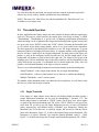
1
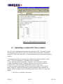
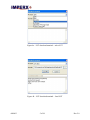
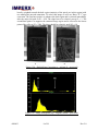
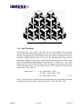
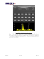
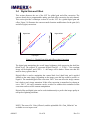
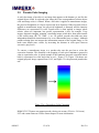
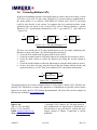
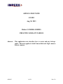
APPLICATION NOTE AN-B03 Aug 30, 2013 Bobcat CAMERA SERIES CREATING LOOK-UP-TABLES Abstract: AN-B03 This application note describes how to create and use look-uptables. This note applies to both CameraLink and GigE cameras Bobcat cameras. 1 of 18 Rev 2.0 1 INTRODUCTION The user defined LUT (Look-Up-Table) feature allows the user to modify and transform the original video data into any arbitrary video data – Figure 1.1. Any 12-bit value can be transformed into any other 12-bit value (if the camera resolution is set to 8-bit or 10-bit, the camera will truncate the corresponding LSBs). The camera supports two separate lookup tables, each consisting of 2048 entries, with each entry being 12 bits wide. The LUT #1 is factory programmed with a standard Gamma 0.45 correction, and the LUT #2 is empty. Both LUT’s are available for modifications, and the user can generate and upload his own custom LUT using the Bobcat Terminal software – refer to “Bobcat user manual CameraUpgrade.pdf” (www.imperx.com) or AN-B01. 12 bit input data LUT 12 bit output data Figure 1.1 - Look Up Table 2 CREATING AND USING LUTs 2.1 Creating LUT with ASCII text editor A custom LUT can be prepared using any ASCII text editor. The file has two main sections: a header and a table. The ‘header’ section is a free text area of up to 256 ASCII characters. Each line of the header section must be terminated in a comma. This header is used to document the LUT and will be displayed in response to the user issuing a ‘glh’ (Get LUT Header) command. The ‘table’ section of the file contains an array of 4096 lines with each line containing an input value followed by a comma and an output value. The input values represent incoming pixels and the output values represent what each incoming pixel should be converted into as an output pixel. After creating the file, rename the file extension to .lut and upload the file. The format of the .LUT file is as follows: AN-B03 2 of 18 Rev 2.0 -- Look Up Table input file example, -- lines beginning with two dashes are comments, -- and are ignored by parser, :Header, -- the text in bold below is the LUT header, -- the text will get displayed with a 'glh' command, Function is 'LUT function', Created by John Doe, Date 12/14/05, :Table, -- the text in bold below is the actual LUT --input output, 0, 10 1, 20 2, 30 : 4095, 4000 2.2 Creating LUT with Microsoft Excel A custom LUT can be prepared using any spreadsheet program similar to Microsoft Excel. The file can be created in Excel as follows (refer to Figure 2.1): 1. Open a new spreadsheet and create the LUT “Header” as explained in section 2.1. 2. Create the actual “Table” by entering the input data values (note that 4096 rows are required in the table ). 3. Add the necessary equations into the output cells to generate the transfer function required. 4. Save the file as a .csv (comma delimited format ). 5. Rename the .csv file to an extension of .lut. 6. Upload the .lut file into the camera. AN-B03 3 of 18 Rev 2.0 Figure 2.1 – Microsoft Excel LUT source file 2.3 Uploading a custom LUT into a camera The LUT can be uploaded into the camera using the Bobcat GUI - Download Terminal. The camera has a place for two LUTs, but only one can be used at a time. To upload a custom LUT follow the steps bellow. For more information refer to the camera manual or AN-B01. 1. Start Application Bobcat CamConfig go to Main Menu and from submenu “Load From…” select “Factory Space”. Wait until camera is initialized. 2. Go to Main Menu and from submenu “Terminal”, select Download Terminal. 3. When “Download Terminal” is opened, from File Type, you have to select the LUT#1 or LUT #2 file you want to upload to the Camera – Figure 4a,b. 4. When you select the appropriate file for this particular camera you have to press button “Load File” and wait to finish the process of uploading. This could take few minutes. When everything is done you should get the message “Done!” Re-power the camera. 1. Re-power or “Soft Reset” the camera. AN-B03 4 of 18 Rev 2.0 Figure 4a – LUT download terminal – select LUT Figure 4b – LUT download terminal – Load LUT AN-B03 5 of 18 Rev 2.0 3 USER DEFINED LUT – EXAMPLES 3.1 Gamma Correction The gamma () correction is a nonlinear modification of the slope of the camera transfer function, which results in the suppression or enhancement of certain image regions. This correction has a smooth curve (compared to knee correction), which allows more precise control over the image correction – Formula 3.1 ( is the desired correction level). Figure 3.1 illustrates this nonlinear conversion for different gamma values. Initially gamma correction ( = 0.45) was introduced in analog broadcast cameras in order to compensate for the non-linear response of the Cathode Ray Tubes (CRT). In machine vision applications this technique is used to improve the object contrast with respect to the background. The actual gamma value depends on the scene, and more particular on the relation between the object and background brightness levels. This correction yields similar results to the one described in the next section. Output signal = (input signal) (3.1) Figure 3.1 - Gamma Corrected Video Signal The camera has a built-in gamma correction ( = 0.45) in LUT “User 1”, which is based on a modification of formula 3.1 in accordance to the SMPTE standard. AN-B03 6 of 18 Rev 2.0 NOTE: The source file “gamma.xls”, and the uploadable file “gamma.lut” (along with the original files “gamma_45.xls”, and “gamma_45.lut”) are available after registering at www.imperx.com. 3.2 Knee Correction Knee correction is a modification of the slope of the camera transfer function, which results in the suppression or enhancement of certain image regions. Figure 3.2a illustrates some examples of double knee corrections (the number of knee points in not limited). The knee correction curve is formed by two sets of variables – knee points (P1, P2), and slopes (S1, S2). The knee point location determines the range of the correction, and the slope (the tangent of the angle) – the power of the correction. Kn Knee a1 P2 Input signal 3 TF i e ig Or F lT a n TF 4 K ne S2 = tg(a2) P1 2 1 TF F T ee Kn ee S1 = tg(a1) a2 Output signal Knee TF 1 – enhances the dark image regions and suppresses the bright ones. Knee TF 2 – suppresses the dark and bright image parts and enhances the mid range. Knee TF 3 – enhances the bright image regions and suppresses the dark ones. Knee TF 4 – enhances the bright and dark image parts and suppresses the mid range. Output signal 1. 2. 3. 4. Input signal Figure 3.2a – Double Knee Correction The number of knee points, their location, and the correction slope is scene dependent. The best approach for knee point selection is to use the image histogram. A typical histogram consists of multiple peaks and valleys. In common vision applications the user will have a mixture of bright and dark objects and backgrounds. The dark pixels will produce one or several peaks in the histogram located towards the left, and the bright pixels will produce one or several peaks located in the right side. The midrange gray level pixels will produce one or several peaks in the middle of the histogram. If the histogram is weighted towards a particular region, this region needs to be suppressed. Alternatively, if the histogram has a flat region, this region needs to be enhanced. Figure 3.2b shows an original image (left) and processed one (right). Figure 3.2c shows the image histograms before (top) and after (bottom) processing. The dominant brightness level in the original image is black and dark gray (with a very bright bottom section). The image histogram is AN-B03 7 of 18 Rev 2.0 heavily weighted towards the dark region (majority of the pixels are in this region) with two small peaks towards saturation. To correct the image we will use “Knee TF 1” type correction. The first knee point is to enhance the dark region and is selected immediately after the major left peak at P1 = 650. The slope has to be relatively steep S1 = 3. The second knee point is to suppress the saturated image region and is selected in the lowest point of the valley at P2 = 2200. The slope should be relatively small S2 = 0.8. Figure 3.2b – Double Knee Correction (a – original, b – processed) Figure 3.2c – Image Histograms (top – original, bottom – processed) AN-B03 8 of 18 Rev 2.0 It is clear that after the correction, the image has better contrast in the dark region (the subjects are clearly visible), and the saturation has been eliminated. NOTE: The source file “Dual_Knee.xls, and the uploadable file “Dual_Knee.lut” are available at www.imperx.com. 3.3 Threshold Operation In some applications the binary images are much simpler to analyze that the original gray scale one. The process, which converts the regular gray scale image to binary, is called “Thresholding”. Thresholding is a special case of intensity quantization (binarisation) where the image can be segmented into foreground and background regions, having only two gray scale levels “HIGH” (white) and “LOW” (black). Selecting the threshold value is very critical for the binary image quality, and it is to a great extend scene dependent. The best approach for threshold point selection is to use the image histogram. A typical histogram consists of multiple peaks and valleys. In common machine vision applications the user will have a dark object on a bright background. The dark pixels of the object will produce a peak in the histogram located towards the left, and the bright pixels of the background will produce a peak located in the right side. The relatively few pixels with midrange gray level are around the edge of the object, and they will be responsible for the valley between the two peaks. If a threshold level is chosen within the valley, this will produce a well-defined boundary of the object, which is essential. There are several thresholding techniques based on the number of the threshold points: - Single Threshold – with a single point (known also as simple thresholding) - Dual Threshold – with two points (known also as interval or window thresholding). - Multiple Thresholds – with 3 or more points. The number of the threshold points is not limited, but for simplicity we will discuss only the first two, which are the most common. 3.3.1 Single Threshold If the image is a high contrast scene and has well defined bright and dark regions a simple binarisation technique can be used for thresholding – Formula 3.3.1. The binary image output is converted to “HIGH” (white) for all gray level values higher or equal to the selected threshold point TH, and to “LOW” (black) for all gray levels lower than TH. In such a case the image histogram has two (or more) well-defined peaks, separated by well-defined valleys (“bimodal” type histogram). Finding the threshold value TH in this case is relatively simple, the user has to find the lowest point in the histogram. Figure 3.3.1a shows the original image and its histogram. This histogram is a typical “bimodal” type and the optimal threshold value is ~ 2000. Figure 3.3.1b shows the image after a simple single threshold operation (TH = 2000). AN-B03 9 of 18 Rev 2.0 Output signal => 1 IF (input signal TH) 0 IF (input signal < TH) (3.3.1) NOTE: The source file “Single_Threshold.xls, and the uploadable file “Single_Threshold.lut” are available at www.imperx.com. Figure 3.3.1a – Original image and its histogram AN-B03 10 of 18 Rev 2.0 Figure 3.3.1b – Processed image with single threshold. 3.3.2 Dual Threshold If the image has a low contrast and does not have well defined dark and bright regions, the simple threshold operation does not yield good results. In such images, the image histogram has several (usually small) peaks and not well defined valleys, so selecting a single threshold value is not easy, and the thresholded image will be substantially different based on the threshold point selection. In such cases a dual (interval) thresholding technique has to be implemented – Formula 3.3.2. The binary image output is converted to “HIGH” (white) for all gray level values between the selected threshold interval TH1 and TH2, and to “LOW” (black) for all gray levels outside (TH1, TH2) interval. Output signal => 0 IF (input signal TH1) 1 IF (TH1 < input signal < TH2) 0 IF ( input signal TH2) (3.3.2) Figure 3.3.2a shows the original image and its histogram. From the image histogram the optimum interval location is at the valleys TH1 = 1500, and TH2 = 3000. AN-B03 11 of 18 Rev 2.0 Figure 3.3.2a – Original image and its histogram Figure 3.3.2b shows the image after a dual threshold operation. The loss of information after dual thresholding is minimum. Figure 3.3.2c shows the image after a single threshold operation is performed (TH = 2000). It is clear that the loss of information is much higher. AN-B03 12 of 18 Rev 2.0 Figure 3.3.2b – Processed image with double threshold Figure 3.3.2c – Processed image with single threshold NOTE: The source file “Dual_Threshold.xls, and the uploadable file “Dual_Threshold.lut” are available at www.imperx.com. AN-B03 13 of 18 Rev 2.0 3.4 Digital Gain and Offset This section discusses the use of the LUT for global gain and offset correction. The camera already has a programmable analog gain and offset correction for each channel. This section provides a technique on how to use the LUT for a global digital gain and offset. Figure 3.4 illustrates the camera transfer function modifications for the gain (left) and offset (right) corrections. Output signal Digital Offset D G Output signal Digital Gain F DO DO 1 2 F T al T al in in ig Or ig Or Input signal Input signal Figure 3.4 – Digital Gain (left) and Offset (right) Correction The digital gain manipulates the overall image brightness while preserving the dark bias (black level). The original TF represents Digital Gain DG = 1. If DG > 1 the resultant image will be brighter, and if DG < 1 – the image will be darker. Please note that DG must be always greater than 0. Digital Offset is used to manipulate the camera black level (dark bias) and is applied globally to the entire image. Depending on the image scene the bias could be positive or negative. The standard digital offset correction “DO 1” does not affect the image contrast but it leads to early image saturation. If this offset correction is normalized, as shown on curve “DO 2”, the early saturation can be avoided. In addition this normalized offset correction can be used for contrast manipulation. Digital offset and digital gain can be used simultaneously to perfect the image quality in non-perfect lightning situations. NOTE: The source file “Gain_Offset.xls, and the uploadable file “Gain_Offset.lut” are available at www.imperx.com. AN-B03 14 of 18 Rev 2.0 3.5 Pseudo-Color Imaging A real-color image of an object is an image that appears to the human eye just like the original object would. In a pseudo-color image this close correspondence between object color and image color is violated. When a real-color is applied to monochrome images, the perceived brightness of a object is preserved in its depiction. When a pseudo-color is applied to monochrome image, the perceived brightness is distorted, and the intensity differences are represented via color. Pseudo-color is often applied to images where relative values are important, but specific representation is not, for example, X-ray images, ultrasonic imaging, mapping, visualizing images which have been taken outside of the visible range (IR, UV, radar…), etc.. In general, pseudo-color adds one more independent dimension measurement over a two-dimensional map or image. Although pseudo-coloring does not increase the information contents of the original image, it can make some details more visible, by increasing the distance in color space between successive gray levels. To convert a monochrome image to a pseudo-color one the user has to select the conversion function. This function is the mapping of each pixel luminance (grayscale) value to a particular color. A tipical example is the continous grayscale conversion where balck is represented as violet and white as red – Figure 3.5a. Figure 3.5b shows one original grayscale image captured form UAV, and Figure 3.5c the processed pseudocolor one. Figure 3.5a – Grayscale to Color Correction BOBCAT LUT feature can support pseodo coloring via custom (12 bit in – 24 bit out) LUT and custom firmware. Please contact Imperx for more information. AN-B03 15 of 18 Rev 2.0 Figure 3.5a – Original UAV Image AN-B03 16 of 18 Rev 2.0 Figure 3.5c – Processed UAV Image AN-B03 17 of 18 Rev 2.0 3.6 Cascading Multiple LUTs In the most demanding machine vision applications, to achieve the perfect image, several LUTs have to be used. To date, most common LUT post processing is implemented in the frame grabber or in software. With BOBCAT camera series, all LUT processing could be done directly in the camera. Let suppose that in a particular machine vision application the user needs to use several LUTs, each of them performing a specific function: LUT 1 is performing a function f(x), LUT 2 – g(x), and LUT 3 – h(x), and so on – Figure 3.6a. In LUT 1 In Out LUT 2 f(X) In Out g(X) LUT 3 Out h(X) Figure 3.6a – Cascading Multiple LUTs The user can cascade the LUTs and combine them in one by simply multiplying the functions as shown in Figure 3.6b. When using Microsoft Excel: 2. Create the first column with the input values from 0 to 4095, 3. Create the second column to reflect the function f(x) using the first column as source, 4. Create the third column to reflect the function g(x) using the second column as source, 5. Create the fourth column to reflect the function h(x) using the third column as source. 6. Create a new sheet and copy only the first and the last column, add the header, and export this sheet to .csv file. Thus your combined LUT will perform all functions. In LUT Out f(X)*g(x)*h(x) Figure 3.6b – Combined LUT This application note gives some examples of how to create and use custom LUTs. This does not limit the LUT function set, as many more functions or combinations are possible. Please contact Imperx if you need a specific LUT function implementation. The source files for the examples in this note are available at www.imperx.com. Imperx, Inc. Tel: (+1) 561-989-0006 Fax: (+1) 561-989-0045 Email: [email protected] Web: www.imperx.com AN-B03 Copyright 2013, Imperx, Inc. All rights reserved. Any unauthorized use, duplication or distribution of this document or any part thereof, without the prior written consent of Imperx Corporation is strictly prohibited. 18 of 18 Rev 2.0