Download Keypoints Manual

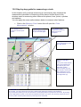
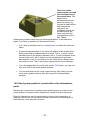
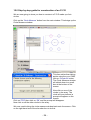
ABERLINK 3D MKIII MEASUREMENT SOFTWARE
PART 1 (MANUAL VERSION) COURSE TRAINING NOTES
ABERLINK LTD.
EASTCOMBE
GLOS.
GL6 7DY
UK
INDEX
1 .0 Introduction to CMM measurement .......................................................4
2.0 Preparation and general hints for solving measurement problems ....4
3.0 Starting up your machine ........................................................................5
3.1 Referencing the machine........................................................................5
3.2 To reference the machine.......................................................................5
4.0 Probe Calibration .....................................................................................7
4.1 Background ............................................................................................7
5.0 Aligning your Parts ..................................................................................9
5.1 Example of traditional part alignment using a surface table, straight
edge and pins. ..............................................................................................9
6.0 Aligning parts using a CMM ....................................................................9
7.0 Alignment examples ..............................................................................10
8.0 Basic 3-2-1(2) Alignment .......................................................................12
9.0 Plane and two circles Alignment ..........................................................13
10.0 Aligning components using a cylinder ..............................................14
11.0 Drive shaft (aligning along shaft’s centre line)..................................16
12.0 How accurate is your CMM ? ..............................................................18
13.0 Step by step guide for measuring a circle .........................................20
14.0 Step by step guide for construction of an intersection point...........21
15.0 Step by step guide for construction of an P.C.D ...............................24
16.0 Bring up Dimensions on the Screen..................................................26
17.0 Selecting Features ...............................................................................27
18.0 Using the Feature Select Buttons ....................................................28
19.0 Aligned Dimensions.............................................................................29
19.1 3D Dimensional ..................................................................................29
19.2 2D Dimensional ................................................................................31
20.0 Horizontal and Vertical Dimensions ...................................................31
21.0 Angular Dimensions ............................................................................32
21.1 3D Dimensional Angles ......................................................................32
21.2 2D Dimensional Angles ....................................................................33
22 .0 Dimensioning Circles..........................................................................35
22.1 Displaying the form of a Line or a Plane .............................................35
23.0 Displaying a Feature as a Datum ........................................................36
24.0 Displaying the position of a Circle, Point or Sphere .........................37
25.0 Dimensioning between two Lines or Planes......................................38
26.0 Dimensioning to a Cone ......................................................................38
27.0 Setting Nominal Values and Tolerances for Dimensions .................39
28.0 Geometrical Tolerances.......................................................................41
29.0 Recalling a measured Unit ..................................................................41
30.0 Printing the Results .............................................................................42
30.1 Graphic Print outs ...............................................................................44
30.2 Tabulated Units...................................................................................44
30.3 Tabulated Dimensions ........................................................................45
31.0 Geometrical Tolerances Summary .....................................................49
31.1 Introduction to Geometric Dimensioning and Tolerancing ..................49
31.2 Geometric Tolerancing in Aberlink......................................................50
32.0 Geometric Characteristic Symbols.....................................................51
32.2 Flatness ..............................................................................................52
32.3 Roundness or Circularity ....................................................................52
32.5 Cylindricity ..........................................................................................52
- II -
32.6 Parallelism ..........................................................................................53
32.7 Angularity............................................................................................53
32.8 Squareness ........................................................................................54
32.9 Concentricity.......................................................................................54
32.10 Total Runout .....................................................................................54
32.11 True Position.....................................................................................56
32.11.1 True Position relative to specified datum(s)....................................................... 57
32.11.2 Maximum Material Condition.............................................................................. 59
32.12 Symmetry .........................................................................................60
32.13 Profiles..............................................................................................62
33.0 Change History....................................................................................63
34.0 Contact Details .....................................................................................63
- III -
1 .0 Introduction to CMM measurement
The goal of this training document is to show you, by use of easy-tounderstand examples, how to set up the cmm and measure parts.
This training manual also helps you to get familiarized with Aberlink 3D
general rules, definitions and terms and shows you how to apply these to your
specific measurement problems.
These training notes contain some of the most important points to help
support you during this training course, it does not replace the use of the
Aberlink user manual. In fact we highly recommend you read the user manual
in spite of successful training, as not all measurement capabilities of this
software can be covered in this training course.
It is important that you take your own notes throughout. If you have any
questions about training, always ask questions immediately to help contribute
to the success of your training.
2.0 Preparation and general hints for solving measurement
problems
Before you start measuring with your cmm you must go through some
preparation functions. Those function include:
•
Give some thought to how you are going to position and hold the part.
Reason:
- Probe accessibility
•
Decide which stylii and extensions, if any, you may need, and if you are
using an indexible head, which probe angles you are going to need to
measure the part, before you start.
Reason:
- Save time while programming
- Saves you having to move the part
•
It’s good working practice to write the feature numbers on the drawing.
Reason:
- Easy verification of the inspection report
- Useful guidance when running a part inspection
program
-4-
3.0 Starting up your machine
Air supply:- Check your CMM has a minimum air supply of 3.9 bar (55 psi)
and the filters (pots) are free of oil and water contamination (oil and water
must never get through to air bearings as this could damage your
machine).
Air on and axes locking switches:- on the top of the right hand column is a
set of four switches. These are used to switch on the main air supply and to
individually lock the cmm axes.
X axis lock
Y axis lock
Z axis lock
Main air supply
On / Off switch
Taking points:- It is perfectly acceptable to roughly position the probe head
by hand but you must always take points with the fine adjust knobs.
3.1 Referencing the machine
Each time the computer is switched on, before you can start to measure with
your CMM, the machine has to be referenced.
If the computer is left switched on, you do not have to re-reference the
machine each time you start the software.
3.2 To reference the machine
Gently move all three axes in a positive direction, until they reach their
physical stops. (top right-hand corner). This corresponds to pushing the X
axis to the right, the Y axis to the back and the Z axis to the top of the
machine.
-5-
Click the ‘OK’ button on the
reference window. The machine
is now referenced.
To re-reference the machine at any time press the ‘Machine Reference’ button
and repeat the above process.
Notes
-6-
4.0 Probe Calibration
4.1 Background
When using the Aberlink 3D software to inspect a component, the software
must know the relative position and diameter of the stylus ball being used.
This is achieved by using the probe stylus ball to measure the reference ball,
which is mounted on the granite table. As the size and position of the
reference ball are known, this measurement is used to determine the size and
relative position of the stylus ball. This information is stored as three position
offsets X,Y and Z, and a diameter.
Obtaining this information is known as calibrating the probe. The probe must
be calibrated every time you change a stylus or, if you have an indexible
probe, each time you move the probe head to a position that has not
previously been calibrated.
If you are using a Renishaw indexible probe, it is advisable to datum the
probe head at all relevant positions prior to commencing your inspection.
To calibrate the probe left click with the mouse on the
green area in the Probe Head icon to call up the Probe
Status window.
Calibrated probe / stylus data
window.
Probe to be datumed window.
-7-
1. To datum a probe position select the A (incline) and B (rotation) angles
you require, by using the drop down menus located at the bottom left
hand side.
2. Press the ‘Add’ button in the right corner of the Probe Status window,
you should then see a line in the ‘Datumed Positions’ window showing
the probe position you want to calibrate.
3. Move the probe head to match the selected A and B probe positions.
With the probe in correct position take a minimum of five points around
the reference ball, which is attached to the granite surface. The first
point should be on the pole (TDC) of the ball, with the remainder of
points being spread evenly around the equator. (Note – with
whichever probe position you are datuming, you will only ever be
able to access one half of the reference ball. Try to spread the
points taken evenly around this area).
4. If successful, the calibrated probe position will appear as a line in the
stylus data window and the indicator button will turn green in colour. If
the probe position does not turn green, or you are not happy with any
point that you have taken, you can erase the last point taken by left
clicking on the ‘Retake’ button or erase all of the points taken by left
clicking on the lowest ‘Clear’ button.
To repeat this process press ‘Clear’ in the Datumed Positions window and
select the new A and B angles you require.
Repeat this process until all the required probe positions have been datumed,
and then click ‘OK’. This brings back the Main Screen.
To change to another datumed probe position
Left click on the Probe Head window and then left click on the datum probe
position you want in the Calibrated Probe window.
The red dot will turn green (this shows the probe position has been selected)
click on ‘OK’.
A window will appear telling you to manually change the A and B Angles on
the probe head. (The A and B angles shown in the software and the A and
B angles of the probe must be the same before measuring anything).
Notes
-8-
5.0 Aligning your Parts
5.1 Example of traditional part alignment using a surface table, straight
edge and pins.
When you place a part on a surface table you are aligning the bottom face of
that part true to the top of the surface table, you can still move the part about
in the X-Y plane and rotate it about the Z axis but you cannot move it up and
down in the Z axis or rotate it around the X or Y axis, this is called a primary
alignment.
Push the part up to a straight edge fixed to the surface table this will stop any
rotation about the Z axis as well as any movement along the Y axis, now you
can only slide the part along the X axis.
This is called a secondary alignment.
Now slide the part along the X axis up to a pin in the surface table.
The part is now fixed in all six degrees of freedom it cannot move or rotate in
X Y or Z.
6.0 Aligning parts using a CMM
When using the CMM to inspect a component, it is not necessary to physically
align the component to the axes of the machine. By measuring specific
features on the component and setting them as references, you will be able to
use the computer to define the orientation of the axes and position of the
component.
This is important when measuring 2 dimensional shapes ie. lines and circles,
or points, as the software will project the measurement points into a plane
which must be fully defined. Also the alignment of the component must be
properly defined in order to produce meaningful horizontal and vertical
dimensions on the screen.
-9-
7.0 Alignment examples
When you place the component on the table of the machine it has six degrees
of freedom which will need to be defined, in order to fully define the alignment
and position of the component. Namely these are translation along, and
rotation about, each of the three axes.
Depending on what measurements you wish to perform, not all of these
degrees of freedom will necessarily have to be defined. Take for example a
cube with a hole in it’s top and front faces:
Z
Y
X
Measure a plane on the top face of the cube and set it as a reference. This
defines the XY plane for the cube and also a Z zero position. In effect it
defines three of the degrees of freedom, which are rotations about X and Y,
and also translation in Z.
Next measure a line along the front edge of the cube and set it as a reference.
This now defines the XZ plane for the cube and also a Y zero position. In
effect this line defines a further two of the degrees of freedom, which are
rotation about the Z axis and also translation in Y. Note that this line will now
be used to define the plane if the hole in the front face is now measured as a
circle.
Now measure the hole in the top face of the cube as a circle and set this as a
reference. The software will automatically determine that the hole is in an XY
plane by looking at the direction of motion of the probe. Setting this circle as a
reference will set the centre of the circle to X=0, Y=0 and define the last
outstanding degree of freedom ie. translation in X. The position and alignment
of the block will now be fully defined.
Note that a plane, a line and a circle are the most common features used to
fully define a component. Only one reference of each type can be set, it is
also recommended that when creating a program references are not altered.
If the component being measured does not include these features other
common features that can be used as references are as follows:
- 10 -
1. No straight edge for alignment
1. Measure circle – Set Ref
2. Measure circle – OK
3. Construct Line – Set Ref.
2. No Suitable Hole
2. Measure line
– OK
3. Construct Point – Set Ref
1. Measure line – Set Ref
In summary, the six degrees of freedom for a component are usually fully
defined by referencing a plane, a line and a circle (or point). Different features
when referenced will define various degrees of freedom, and this is more fully
discussed in appendix 1.
It is worth noting before finishing this chapter, that cylinders and cones when
referenced will define four degrees of freedom. Take a cylinder that has been
referenced to define the X axis of the component.
Z
Y
X
- 11 -
The axis of the cylinder defines both the rotations about, and the translations
along the Y and Z axes. This can be a useful technique for defining the
orientation and position for turned components.
8.0 Basic 3-2-1(2) Alignment
To measure a block type component like the Aberlink testpiece
Y
Z
1.) Measure at least four
points on top face Primary
Alignment
X
1. Measure a plane on the top of the block, by clicking on the ‘Plane
Measure’ button. When the Plane Measure window opens take four
points on the top face (Plane 1). Press the ‘Set Ref’ button (this will
align the Z axis 90° to the measured plane - this is our Primary
alignment), then click ‘OK’.
2. Next measure a line along the side of the block, by clicking on the ‘Line
measure’ button. When the Line Measure window opens take three
points along the side of the part (Line 2). Press the ‘Set Ref’ button
(this will rotate the axes system to align the Y axis to the side of the
part this is our secondary alignment), then click ‘OK’.
3. The last thing we need to do is to measure a line along the back face of
the part, by clicking on the ‘Line Measure’ button when the Line
Measure window opens take three points along the back face of the
part (Line 3). Press the ‘Set Ref’ button (this will create an origin (zero
point) in the corner where the two lines intersect each other on the top
face) then click ‘OK’.
Notes
- 12 -
9.0 Plane and Two Circles Alignment
Measure a circle (2) in one of the
small bores in the top face. Press
‘Set Ref’ button this now your origin
(zero point)
Measure a plane (1) on the top
face press ‘Set Ref’ button this is
now your Primary alignment
Construct a line (4) joining the
centres of the two circles (2 and 3).
Press the ‘Set Ref’ button - this is
now your secondary alignment.
Measure a circle (3) in the
opposite small bore in the top
face. Do not press the ‘Set Ref’
button.
1. Measure a plane on the top of the block, by clicking on the ‘Plane
Measure’ button when the ‘Plane Measure’ window opens take four
points on the top face (Plane 1). Press the ‘Set Ref’ button (this will
align the Z axis 90° to the measured plane - this is our Primary
alignment), then click ‘OK’.
2. Measure a circle, one of the small bores, by clicking on the ‘Circle
Measure’ button. When the ‘Circle Measure’ window opens take four
points in one of the small bores (circle 1). Press the ‘Set Ref’ button,
this now is your origin (zero point).
3.
Measure the small bore opposite the one you just measured, by
clicking on the ‘Circles Measure’ button when the Circle Measure
window opens take four points (circle 2). Do not press the ‘Set Ref’
button as we are going to use this circle to construct a line.
4.
The last thing we are going to do is to align the Y axis of the cmm to a
constructed line between the two circles by clicking on the ‘Line
measure’ button when the Line Measure window opens. Click on the
‘Construct’ button then select circle 1 by left clicking on it in the graphic
window, you will now see a window which asks you if you want to
construct a line between two points click ‘YES’ select the other circle in
- 13 -
the same way by left clicking on it in the graphic window, you now have
a constructed line, press the ‘Set Ref, button and then click ‘OK’, this
will align the Y axis along the constructed line, this our secondary
alignment.
Notes
10.0 Aligning components using a cylinder
To measure a flange type component
3
100 mm Dia
Z Axis
2
10 mm Dia
Y Axis
1. Place the part on the table with the 100mm diameter facing up and two
of the 10.0 mm holes aligned along the Y axis of the cmm.
2. Measure the 100 mm O/D as a cylinder by clicking on the ‘Cylinder
Measure’ icon with the left mouse click, when the ‘Cylinder Measure’
window opens take four points at the top of the cylinder in a circle and
four points around the bottom of the cylinder. Press the ‘Set Ref, and
then click ‘OK. ’ The Z axis is now aligned to the centre line of the
cylinder.
3. Measure a plane on the end of the 100 mm cylinder, by clicking on the
‘Plane Measure’ button when the Plane Measure window opens take
- 14 -
four points on the top of the 100mm cylinder do not press the ‘Set Ref’
button (this will be used as the working plane to project the point into)
and click ‘OK’.
5
Y Axis
X Axis
4
1. Next we are going to construct a datum at the point where the cylinder
meets the plane (X,Y datum centre of cylinder, Z datum on top plane).
Click on the measure ‘Point Button’ when the measure point window
opens click on the ‘Construct Button’ then select the plane by left
clicking on it in the graphic window, you will now see a window asking
you if you want to construct a intersection point click ‘YES,’ select the
cylinder by left clicking it in the graphic window, you have now
constructed a point, press the ‘Set Ref’, and then click ‘OK’ this zeros
X,Y and Z axes.
2. The last thing we need to do is to align the Y axis through one of the
10mm holes. Click on the measure ‘Circle Button’ when the measure
circle window opens take 4 points in the 10mm hole at the 12 o’clock
position then click ‘OK’ you now have a 10mm circle in our working
plane. We are now going to align the Y axis of the cmm via a
constructed line between the datum point and the 10mm hole. Click on
the measure ‘Line Button’ when the measure line window opens, click
on the ‘Construct Button’ then select the datum point by left clicking on
it in the graphic window, you will now see a window which asks you if
you want to construct a line between two points click ‘YES.’ Select the
circle in the same way by left clicking on it in the graphic window, you
now have a constructed line, press the ‘Set Ref’, button and then click
‘OK’ to align the Y axis along the constructed line.
The component is now aligned true to the centre line of the 100mm cylinder
(Primary Alignment) with the Y axis going through the 10mm hole
(Secondary Alignment) with the X, Y, Z axes zeroed where the cylinder
meets the top face.
- 15 -
11.0 Drive shaft (aligning along shaft’s centre line)
Place the shaft on the cmm table with the shaft facing down the table (along
the Y axis)
1
2
4
X Axis
Y Axis
CMM Table
As main datum is the centre line of the shaft we need to align the Y axis of the
cmm to the centre line to do this:1. Click on the measure ‘Plane Button’ when the Measure Plane window
opens take four points on one end of the shaft click ‘OK’, this is plane
1.
2. Click on the measure ‘Circle Button’ when the measure circle window
opens take four points around the end of the shaft by plane one, circle
(2) is automatically projected into plane 1. Press the ‘Set Ref’ button
this sets the XYZ datum on this end of the shaft (Zero point) click ‘OK’.
3. Repeat this process for the other end of the shaft but do not press the
‘Set Ref’, button this time you now have one plane and one circle at
each end of the shaft, we can make a centre line by joining these two
circles together (constructed) and by pressing ‘Set Ref’ this is our
(Primary alignment).
4. To do this click on the measure ‘Line Button’ when the measure line
window opens, click on the ‘Construct Button’ then select one of the
circles by left clicking on it in the graphic window, you will now see a
window which asks you if you want to construct a line between two
points, click ‘YES’ select the other circle in the same way by left hand
clicking on it in the graphic window, you now have a constructed line.
Press the ‘Set Ref, button and then click ‘OK’ this will align the Y axis
along constructed line.
- 16 -
If the shaft has any cross holes, keyways or flats these can be aligned to one
of the other axes (Secondary Alignment, Timing)
To do a Secondary Alignment using a cross hole measure the cross hole as a
cylinder press the ‘Set Ref’ button, click ‘OK’ this will align either the Z or X
axis to the centre of the cylinder
X Axis
Y Axis
To do a secondary alignment using a keyway or flat measure the bottom of
the keyway or flat as plane press the ‘Set Ref’ button click ‘OK’ this will align
either Z or X axis to a line 90 deg to the plane.
X
If you use a plane as an
alignment feature to a
axis, this is aligned at 90
deg to the plane
Y
The component is now aligned true to the centre line of the shaft (Primary
Alignment) with the Z or X axis going through the cross hole or at 90 deg to
the flats (Secondary Alignment) with the X, Y, Z axes zeroed in the centre of
the shaft at the front end.
Notes
- 17 -
12.0 How accurate is your CMM ?
Your CMM is a very
accurate instrument
and in the right
circumstances a
cmm is capable of
measuring to within
a few microns, this
is a very small
value.
So how small is a
Micron?” Well, here
is the answer:
A micron, short for
micrometre, is a unit
of measurement
equal to one
millionth of a metre.
A micron is actually
(1 millionth)
0.000001 of a meter
or 0.000039 of an
inch.
To give you some idea, a human hair is 40 to 120 microns in diameter.
Because we are measuring to such a high accuracy, the machine location and
it’s environment is very important and has an influential effect on the
measured result.
If the temperature is too high the parts will expand or if the temperature low
the parts will shrink by different amounts depending on the material they are
made from.
Aberlink 3D can compensate for this within the software, by clicking on the
‘User Definable Parameters Button’ (top of the screen) then clicking on the
‘General Tab’.
Automatic temperature compensation is available as an upgrade. Please enquire to
Aberlink for further information.
- 18 -
Temperature (deg C)
If you wish to compensate for
temperature, then measurement results
are recalculated to what they would be
o
at 20 C (industry standard). Enter the
mean ambient temperature here.
However, you must now enter the
material (and thermal expansion
coefficient) for the component being
measured
Material
As the cmm structure is made from a
single material (Aluminium), it will expand
and contract uniformly with temperature.
It is therefore possible to compensate for
the ambient temperature of the machine
in the software providing that the material
(and thermal expansion co-efficient for
the material) is also known. Select the
material of the measured component from
this list.
Thermal Expansion Coefficient (ppm)
If you have selected ‘other’ from the material list above
then you must enter the thermal expansion coefficient in
ppm for the material here.
Notes
- 19 -
13.0 Step by step guide for measuring a circle
In this chapter we’ll go though measuring a circle step by step, because the
measurement windows for measuring circles have a similar layout to the
windows used for measuring other features like planes, lines, points, cylinders
and spheres.
You can apply the same method shown below to measure other features.
•
Click on the ‘Measure Circle’ button this will open the ‘Circle
Measurement ‘ window
The ‘Retake’ button
removes the last point
taken
The ‘Clear’ button
removes all the points
so you can start again
The ‘Delete’ button
deletes the measured
feature from the
computer
When you have finished
your measurement click
the ‘OK’ button
This is the ‘Set Ref’
button.
If you press it the feature
you just measured will
be used as part of an
alignment system.
(You normally only use
the ‘Set Ref’’ three times
at the beginning of the
measurement to set the
part alignment up).
The ‘Plane’ button
If you wish, you can project the circle into a plane other than that chosen by the software.
If you press the button you can choose which of orthogonal planes to project the circle into. By clicking
on the appropriate XY,XZ or YZ button that defines the plane you want, you can also project the circle
in to any other relevant plane that has previously been measured.
- 20 -
Take four points
evenly spaced around
the circumference of
the central bore. The
depth of the
measurement points
does not matter, as
long as at least half the
ball is below the
surface of the
workpiece so that the
measurements are
taken using the full
circumference of the
ball. These
measurement points inside the hole will be projected on to the reference
plane (Top Face) to produce a 2 dimensional circle.
•
If you take a bad point use the ‘re-take button’ to delete the last point
taken.
•
A pictorial representation of the circle will appear in the window after
three points and be updated after the fourth. The X, Y and Z values
tabulated next to the graphic represent the X, Y and Z positions of the
centre of the circle. As no feature on the workpiece has yet been
datumed the X and Y co-ordinates for the circle will be referenced to
the machine zero. The D value given represents the circle diameter.
•
If you are happy with your circle click on the ‘OK’ button, you can now
see your circle in the main graphic window.
•
You can add points to the circle at any time by right clicking on the
circle in the graphic window (this will re-open the measurement
window).
14.0 Step by step guide for construction of an intersection
point
Because the measurement windows have similar layouts you can use the
same method to construct other features like centre lines and mid points.
Points of intersection can be constructed not only at the intersection of
features which touch, but can also be used to produce the closest point to
both features, when they do not touch.
- 21 -
•
To construct such a point, click on the ‘Point Measure’ button, from the
main screen. This will bring up the ‘Point Measure’ window. Now click
on the ‘Construct’ box and the ‘Point Measure’ window will now shrink
to a small box at the bottom of the screen.
•
Now simply select the features, whose intersections create the desired
point, by clicking on them. After you have selected the first feature a
prompt will appear, to confirm what is happening:
•
Click on ‘OK’, and then click on the second feature. Now the ‘Point
Measure’ window will automatically reappear. The graphics part of the
window and the ‘Points Fit’ box will of course be blank, but the X, Y and
Z co-ordinates of the constructed point will be displayed in red.
- 22 -
•
You may now click on ‘OK’ or ‘Set Ref’ as appropriate, as for any point.
The screen will now return to the Main Screen, and the point will form a
part of the graphical representation.
Notes
- 23 -
15.0 Step by step guide for construction of an P.C.D
We are now going to show you how to construct a P.C.D made up of six
circles.
Click on the ‘Circle Measure’ button from the main window. This brings up the
Circle Measure window:
This time rather than taking
points using the your CMM,
click on ‘Construct’ button.
The Circle Measure window
will shrink down to a small
box at the bottom of the
screen.
Now click on one of the
circles in the array. The
circle will turn pink and a
prompt will appear on the
screen:
Click on ‘PCD’ then click on ‘OK’ and the prompt will disappear.
Now click on all the other circles in the array.
We now need to bring the circle measure window back onto the screen. Click
on the right hand end of the shrunken box to do this.
- 24 -
Click on the right hand end of the
shrunken box to open window
The window will reappear with a circle now constructed through the array.
Click on ‘OK’. To close the window and return to the main screen.
Notes
- 25 -
16.0 Bring up Dimensions on the Screen
One of the nice features of the Aberlink 3D software is that the dimensions for
the measured component can be brought up on it’s graphical representation,
in the same way as they are shown on the component’s engineering drawing.
To bring up the
dimensions onto the
screen all you have to
do is select the features
that you wish to
measure between, by
left mouse clicking on
their graphical
representation. If the
software doesn’t default
to the type of
measurement that you
want (horizontal, aligned
etc.), then you will also
have to select the
correct dimension type.
In most cases the order in which you select the features will make no
difference. The instances in which the order of selection does make a
difference are highlighted later in this chapter.
It is important to grasp the following principles when bringing up dimensions:
1. Circles and spheres are treated as single points in space, with all
dimensions being to their centre. (You can use the Max or Min options
in the ‘Dimension Details’ window to measure to the outside or inside of
a circle).
2. Cylinders are treated as a 3 dimensional line along their axes. When
dimensioning between two lines (or cylinders etc.) the order of their
selection is important.
3. Cones may be treated either as a line along it’s axes, or as a point at
it’s apex, depending on whether the cone is selected as the first or
second feature.
4. When linearly dimensioning a feature to a plane or a line, the
dimension will be perpendicular to the plane or line. When
dimensioning between two planes or lines the order of their selection is
important.
- 26 -
17.0 Selecting Features
When bringing up dimensions on the screen, it is necessary to select the
features that you wish to dimension in the graphical representation.
To select a feature, left click on the dark blue outline of the feature. Make sure
that at the point that you click on the feature there are no other overlapping
features within the selection box.
SELECT
NOT
HER
Note – You cannot select a 3 dimensional feature by clicking on the grey
lines that represent it’s depth.
If you are dimensioning in the side view of a reference plane, which has
had 2 dimensional features projected into the plane, then a single line
on the graphics will represent both the plane and the other features. In
this instance clicking on the line may select any one of the features. To
define the specific feature required you must use the feature select
buttons.
Notes
- 27 -
If you have trouble selecting a feature there are various courses of action.
You can use the
feature select
buttons to assist
selection of the
feature.
18.0 Using the Feature Select Buttons
In some instances it will be difficult to select a feature by clicking on it directly.
For instance, the same line will represent both the side view of a circle, and
also the plane into which it is projected. If you have difficulty in selecting a
feature, the Feature Select buttons will provide the solution.
The red number (initially zero) refers to the feature number in the order that it
was measured. For instance if you measured a plane first, followed by a circle
and then a line, the plane would be feature number 1, the circle number 2 and
the line number 3. The right and left arrows are used to increment and
decrement the feature number, to obtain the feature desired.
If you know the number
of the feature that you
require to select,
simply type it in over
the existing number
and then click on it. So
that you don’t have to
memorise the order
that the features are
taken in, when the
feature number is
selected, the graphical
representation of that
feature will become
red.
- 28 -
Left click on any part
of the view that you
are dimensioning in
(even the white
background or on top
of another feature),
and the highlighted
feature will be
selected.
The Feature Select button will only work to select a feature once. If you need
to select the same feature twice (for instance to display the diameter of a
circle), simply click on the red number again to re-highlight that feature. (This
removes the necessity to use the right and left arrows to move off, and return
to the desired feature). Now left click in the view again to re-select the feature.
19.0 Aligned Dimensions
19.1 3D Dimensional
An aligned dimension can be described as either the shortest distance
between two points in space, or as the perpendicular distance between a line
(or cylinder or plane) and a point. If the 2 features being dimensioned are not
in the same plane this will produce a 3 dimensional aligned dimension.
When selecting any
two features, the
software will
automatically default
to producing a 3
dimensional aligned
dimension. Care must
therefore be taken if
the features are in
different planes as the
dimension produced
may look like a 2
dimensional distance
when shown in one of
the 2 dimensional
views.
- 29 -
These leader
lines can be
positioned at
any length on
either side of the
features by
moving the
cursor on the
screen. When
they are at a
convenient
position click for
a third time. The
aligned
dimension will
now appear.
Note that as the
2 circles being
dimensioned are
in different
planes, the
aligned
dimension is 3
dimensional.
This is best
shown by
bringing up the
same dimension
in the other two
views.
- 30 -
19.2 2D Dimensional
Select the two circle features as before, but this time before placing the
dimension on the screen.
Right click with the
mouse, this will reveal
‘Dimension Type’ drop
down menu.
Scroll down the menu
and select 2D
Alignment.
Then left click to place
the dimension on the
screen.
Note that the 2D and
3D aligned dimensions
will appear identically
in the 2 dimensional
views, although having
different values. Care
should therefore be
taken when
dimensioning between
features that are not in
the same plane.
20.0 Horizontal and Vertical Dimensions
A horizontal or vertical dimension can be described either between two points
in space, or between a line or plane and a point, in which case the dimension
will be attached to the mid-point of the line or plane. Instead of being aligned
between the features, these measurements will be perpendicular to the
alignment of the component (which is defined by setting references). If no
reference has been set, then the axes of the machine will be used.
- 31 -
Note – If the alignment of the component has not been defined,
and the horizontal and vertical dimensions are perpendicular to
the axes of the machine, these measurements will have little or
no significance.
A horizontal or vertical dimension can also be described between two lines, or
two planes, but in this
case the dimension
will attach to the mid
point of the first line or
plane selected only,
and gives their
separation in the
direction
perpendicular to this
line or plane.
When selecting two
points (or circles or
spheres) to dimension
between, or a line and
a point (or equivalent)
the software will
automatically default to producing a 3D aligned dimension. A horizontal or
vertical dimension must be defined as follows:
Select the features between which you wish to dimension, as for aligned
dimensions. The features will turn pink and the outline of some aligned
dimension leader lines will appear. Before positioning the dimension, right
click to bring up the ‘Dimension Type’ menu. Select horizontal or vertical as
required. When the software returns to the main screen the outline of the
dimension leader lines will show the horizontal or vertical dimension, as
selected.
These leader lines can be positioned at any length on either side of the
features, as for aligned dimensions, by moving the cursor on the screen.
When they are at a convenient position click the mouse for a third time and
the dimension will appear on the screen.
21.0 Angular Dimensions
21.1 3D Dimensional Angles
Angular dimensions may be created between two lines or two planes, or
between a line and a plane. Any combination of these features will create an
included angle, which may be dimensioned irrespective of the alignment of
the component. As with aligned dimensions, if the features are not in the
same plane, the angle created will be 3 dimensional.
Select the features between which you wish to dimension; the features will
again turn pink if correctly selected. The software may now default either to an
angular dimension or an aligned dimension, depending on what the angle
between the features is and the outline of the appropriate dimension leader
- 32 -
lines will appear on the screen. If the software has correctly selected an angle
dimension, the leader lines can be positioned at any length in any quadrant of
the angle, by moving the cursor on the screen. When they are at a convenient
position click the mouse and the dimension will appear on the screen.
If however, the
software selected
an aligned linear
dimension, you
must use right
mouse button to
bring up the
‘Dimension Type’
menu, prior to
positioning the
dimension.
Select 3D
Angular
Dimension.
When the
software returns
to the main
screen the
outline of the angular dimension leader lines will now be showing a 3D angle.
You can now position the dimension as previously described.
21.2 2D Dimensional Angles
It is possible to split angles into the 2 dimensional components of the view in
which it is called up. For instance perhaps you are interested only in the X,Y
component of the angle between the two planes dimensioned above.
Once again repeat as described above but this time select a 2D angle
dimension.
Note that the
2D and 3D
angle
dimensions will
appear
identically in the
2 dimensional
views, although
having different
values. Care
should therefore
be taken when
dimensioning
between
features that
are not in the
same plane.
- 33 -
To display on the screen all geometric tolerance values relevant to the
inspection simply click on the Geometric Tolerance button.
The geometric tolerance values that are relevant to the measurements on the
screen will now be displayed.
Now to display the geometric tolerances that are relevant to any particular
feature, (for instance flatness of a plane, straightness of a line) left click twice
on that feature and the outline of a leader line will appear. Move the cursor to
a convenient position on the screen, where you would like to site the
dimension, and click for a third time. The geometric tolerance will now appear
on the screen.
Also true position and maximum material condition of circles can be displayed
and datum symbols attached to features as described above.
Note that the Geometric Tolerance button will switch on and off all
geometric tolerances. If you wish to turn off selected tolerances only
this can be done in the Dimension Details window for that tolerance.
- 34 -
22 .0 Dimensioning Circles
The diameter of a circle, sphere or a cylinder may be brought up on the
screen as follows
Select the circle, sphere or cylinder as previously described. If correctly
selected the feature will turn pink.
Note – You cannot select a cylinder by clicking on the grey lines that indicate
it’s depth.
Now select the same
feature again. The
outline of a single
dimension leader line
will appear on the
screen, and this can
be positioned
anywhere on the
screen by moving the
cursor. When it is at a
convenient position,
left click the mouse
and the diameter will
now appear on the
screen.
22.1 Displaying the form of a Line or a Plane
If you wish to display
the straightness of a
line or the flatness of
a plane on the main
screen simply click
on the feature twice
(like calling up the
diameter of a circle),
then move the cursor
to a convenient
position on the
screen before
clicking, to place the
geometric tolerance.
Note that the
Geometric Tolerance button must be switched on.
- 35 -
23.0 Displaying a Feature as a Datum
If a feature has previously been set as a datum it can be shown on the main
screen by attaching
a datum symbol to
that feature. To do
this simply click on
the feature twice
(like calling up the
diameter of a circle),
then move the cursor
to white space on
the screen and right
click. This will bring
up a menu on the
screen as follows
Note that if the
feature has not been
set as a datum then
the ‘Datum’ option
will be greyed out.
Assuming that the feature has previously set as a datum select the ‘Datum’
option and the outline of a datum symbol will appear. Now move the cursor to
a convenient position before clicking again to display the datum symbol on the
screen.
Note that if the
cursor is over a
previously
measured feature
when you right
click (instead of
over white space)
then that unit will
also be recalled
and you will have
to OK that unit
again before
continuing.
Note also that the Datum symbols can only be displayed if the Geometric
Tolerance button is switched on.
- 36 -
24.0 Displaying the position of a Circle, Point or Sphere
The position of a circle, (point or sphere) can be displayed either as it’s
Cartesian or it’s polar co-ordinates, together with it’s geometrical tolerance for
true position.
Select the circle twice as though displaying it’s diameter as described above.
Now right click in white space to bring up the following menu:
You can now select the option that you desire. Note that the position of the
circle will be relative to the datum position selected on the component being
measured.
- 37 -
25.0 Dimensioning between two Lines or Planes
A linear dimension may be produced between two lines or planes by attaching
the dimension to the first line or plane selected, and extending it either
perpendicularly (for an aligned dimension), or horizontally or vertically (for
horizontal and vertical dimensions), until it reaches the mid-point of the
second one.
If the lines or planes are not parallel, different dimensions will be achieved
depending on which line or plane is selected first. The value for run out is
calculated by projecting perpendicular construction lines from the first
selected line, to meet the ends of the second line. The run out will be the
difference between these two values.
A) Selecting the long line first:
L
RUN
OUT
B) Selecting the short line first:
L
RUN
OUT
The first line selected, in effect, becomes the reference line for the
measurement. If you are measuring the distance between a long line and a
short line it will be better to select the long line first.
26.0 Dimensioning to a Cone
A cone is a special case, as when measuring to it, it may be treated either as
a line along it’s axis, or alternatively as a point at it’s apex.
Similarly, its measured diameter has little meaning (as all the measured points
will be below the surface). Therefore selecting the cone twice will not display
its diameter, as for circles, spheres and cylinders, but it’s included angle.
To measure the diameter of a cone at its end requires the construction of
circle at the intersection of the cone with the plane.
- 38 -
When bringing
up dimensions
to a cone, the
cone is treated
either as a line
or a point,
depending on
whether it is
selected as
the first or
second
feature.
If selected
first, the
software will
treat the cone
as a line along
its axis, and
produce a
relevant
dimension
accordingly.
If however, the cone is selected as the second feature, the software will treat
it as a point at it’s apex, and again produce a relevant dimension accordingly.
Notes
27.0 Setting Nominal Values and Tolerances for Dimensions
- 39 -
When printing out inspection reports using Tabulated Dimensions, it is
possible to print out nominal values (and hence measured error) and
tolerance bands (and hence pass/fail statements). If no nominal value has
been set for a dimension, then the software will use the measured value
rounded to the parameter defined in the ‘Machine Set’ up. Here it is also
possible to set the default tolerance.
If however you wish to set a nominal value or tolerance band other than that
defaulted to, this can be done by right clicking on the relevant dimension. This
will bring up the ‘Dimension Details’ window, as follows
10.070
Now the nominal
dimension and
tolerances can be set
by simply typing over
the default values that
the software has
selected.
Note that if the
measured dimension
falls outside of the
tolerance band set,
the background of the
measured dimension
value will become red.
C
When you ‘OK’ this window and return to the main screen, the dimension
leader lines will also appear red on the graphical representation.
Printing out a tabulated dimensions report, it will be possible to show the
nominal value, the error, the upper and lower tolerances and also a pass/fail
statement.
- 40 -
28.0 Geometrical Tolerances
Where relevant, the geometric tolerance applicable to each measurement unit
(e.g. roundness of circles, straightness of lines) will be displayed underneath
the graphical representation of that unit.
Additionally the True Position and Maximum Material Condition for circles may
be obtained as described above.
29.0 Recalling a measured Unit
When you ‘OK’ a measurement unit and the software returns to the main
screen displaying this measured unit, it is not too late to modify the unit by
adding or deleting measurement points, or changing its reference status.
Each measured unit can be recalled by right clicking on the graphical
representation of the feature in the main screen.
- 41 -
30.0 Printing the Results
Whenever you wish to produce a hard copy of inspection results the print
function is used.
This will bring up the following window
All inspection reports will be printed with a border around them, which can
contain information about the part being inspected. This information can be
entered in the border details frame. Note that you are able to modify the
information titles at this screen. The date is entered by default. Your company
name and address (as entered in the Software Set Up) will also be printed on
each page.
There are six different types of inspection report that you can select.
•
Graphic Details- prints results in the same form as the graphic display,
i.e. an XY, XZ, YZ or isometric view of the component and dimensions.
•
Tabulated Units- prints the details of the each feature, similar to the
information in the measure window of that feature.
•
Tabulated Dimensions- prints all dimensions that are added to the
report from the current or previous inspections.
- 42 -
•
Point Positions- prints the co-ordinates of points and the co-ordinates
and size of circles.
•
Feature Profile- prints the graphical representation of how well the
individual points taken fit the theoretical shape i.e. the form of a feature
such as profile of a surface or the roundness of a circle.
•
Multiple Components- prints the measured values for a batch of
components in a single report
Select the type of report that is required by clicking on the relevant option
button.
Printouts can be in either black and white or colour. Again to select which, you
simply click on the relevant option button. Printing in colour can help highlight
dimensions that are out of tolerance.
The Excel button will automatically open Excel (provided that it has been
loaded on the PC) and export the report selected.
On clicking on the ‘Print’ button a preview of the output will be shown on the
screen. Only the first three sheets are shown in the print preview. To bring
one of the back sheets to the front simply click on it. If the text or result
becomes too long for the resolution of the screen then a box containing a
diagonal cross will replace it.
- 43 -
30.1 Graphic Print outs
This is the most commonly used print routine as it closely mimics the output
that the software produces during use. When this option is selected the user
can then select one or more of the four possible views XY, XZ, YZ and ISO for
printing. If more than one view is selected the individual views are printed on
separated sheets. The extent of the area that is printed is based on the
current software view, but as the aspect ratio of the page and screen are
different it is advisable to observe the print preview before continuing with the
print. This will confirm exactly what will be printed, especially useful if key
dimensions are close to the edge of the view. If all necessary dimensions are
not on the print preview then re-zoom the view in the software and recheck
the print preview.
30.2 Tabulated Units
This routine will print the properties of the units that have been inspected e.g.
for a circle unit it’s centre co-ordinates and diameter will be printed or for a
line unit the start and end co-ordinates will be printed, as well as it’s
directional vector. In order for these co-ordinates to have any real meaning
the part origin must have been defined, by referencing the appropriate
features.
- 44 -
30.3 Tabulated Dimensions
The dimensions that have been added to a part inspection can be printed in
tabulated form. This is often more useful than printing Tabulated Units as
these dimensions should be the same as on the original component drawing.
When printing Tabulated Dimension reports, it is possible to select what
information is printed in the report using the check boxes in the Print window.
Note: Unless you have typed in the value of the nominal and tolerance
for each dimension, the nominal values shown will be the measured
values rounded to the rounding tolerance given in the Machine Set Up,
and all tolerances applied will be the default.
- 45 -
Note that both dimensions and geometric tolerances can be toleranced and
hence both have separate pass/fail statements where applicable.
It is possible to add the dimensions from more than one inspection to a
Tabulated Dimensions report, which is why the ‘Clear Report’ and ‘Add to
Report’ buttons appear on the Print window. Every time you click on the ‘Add
to Report’ button, the dimensions that are displayed on the main screen will
be added to the report. This will continue until the ‘Clear Report’ button is
clicked.
30.4 Point Positions
This is a specialised report for printing the position and size of circles or any
other feature that can be likened to a point. For instance, when measuring
2000 holes on a PCB this report allows the size and position of the holes to be
printed out without the requirement to call up dimensions to them all.
- 46 -
30.5 Feature Profile
As a feature is inspected,
the fit of the individual
points to the theoretical
shape is shown in the
picture box on the right
side of the measurement
window. If enough points
are taken then a useful
representation of the true
surface is built up. This
picture can be printed
using the feature profile
routine. When you click
on Print or Print Preview
buttons, the software
asks to click on the
feature you wish to print.
- 47 -
When you click on OK, the feature profile will be displayed as above
30.6 Multiple Components
If when measuring a batch of components using the ‘Play’ function with ‘SPC
All Components’ ticked on, the Aberlink 3D software will collect all the
measured data for the entire batch. These values can be printed out in a
single report using this option
Note that any dimensions out of tolerance will be shown in red.
- 48 -
31.0 Geometrical Tolerances Summary
31.1 Introduction to Geometric Dimensioning and Tolerancing
Geometric Dimensioning and Tolerancing (GD&T) is a universal language of
symbols. GD&T symbols allow a Design Engineer to precisely and logically
describe part features in a way they can be accurately manufactured and
inspected. GD&T is expressed in the feature control frame (Figure 1). The
feature control frame is like a basic sentence that can be read from left to
right. For example, the feature control frame illustrated would read: The 5 mm
square shape (1) is controlled with an all-around (2) profile tolerance (3) of
0.05 mm (4), in relationship to primary datum A (5) and secondary datum B
(6). The shape and tolerance determine the limits of production variability.
-A-
5.0
(1)
(2)
(6)
(4)
(3)
0.05 A B
5.0
(5)
2.0
-B-
Fig 1 Above
There are seven shapes, called geometric elements, used to define a part and
it’s features. The shapes are: point, line, plane, circle, cylinder, cone and
sphere. There are also certain geometric characteristics that determine the
condition of parts and the relationship of features.
The purpose of these symbols is to form a common language that everyone
can understand.
- 49 -
31.2 Geometric Tolerancing in Aberlink
Where relevant, the geometric tolerance applicable to each measurement unit
(eg. roundness of circles, straightness of lines) will be displayed underneath
the graphical representation of that unit.
None of these geometric tolerance values will by default be displayed on the
graphical representation of the component that is built up during the
inspection.
To display on the screen all geometric tolerance values relevant to the
inspection simply click on the ‘Geometric Tolerance’ button. The geometric
tolerance values that are relevant to the measurements on the screen will now
be displayed.
To display the geometric tolerances that are relevant to any particular feature,
(for instance flatness of a plane, straightness of a line) click twice on that
feature and the outline of a leader line will appear. Move the cursor to a
convenient position on the screen, where you would like to site the dimension,
and click . The geometric tolerance will now appear on the screen.
- 50 -
true position and maximum material condition of circles can be displayed and
datum symbols attached to features.
Note that the Geometric Tolerance button will switch on and off all
geometric tolerances. If you wish to turn off selected tolerances only
this can be done in the ‘Dimension Details’ window for that tolerance.
32.0 Geometric Characteristic Symbols
32.1 Straightness
— A condition where all points are in a straight line, the tolerance
specified by a zone formed by two parallel lines.
To display the straightness of a line click twice on the line and the
outline of a leader line will appear. Move the cursor to a convenient
position on the screen, where you would like to site the dimension, and click.
The geometric tolerance will now appear on the screen.
- 51 -
32.2 Flatness
— All the points on a surface are in one plane, the tolerance
specified by a zone formed by two parallel planes.
To display the flatness of a plane click twice on the plane and the outline of a
leader line will appear. Move the cursor to a convenient position on the
screen, where you would like to site the dimension, and click. The geometric
tolerance will now appear on the screen.
32.3 Roundness or Circularity
— All the points on a surface are in a circle. The tolerance is
specified by a zone bounded by two concentric circles.
If the geometric tolerance button is switched on, the roundness of a circle will
be displayed automatically underneath the diameter in the graphic window.
32.5 Cylindricity
— All the points of a surface of revolution are equidistant from a
common axis. A cylindricity tolerance specifies a tolerance zone
bounded by two concentric cylinders within which the surface must
lie.
- 52 -
If the geometric tolerance button is switched on, the cylindricity of a cylinder
will be displayed automatically underneath the diameter in the graphic
window.
32.6 Parallelism
— The condition of a surface or axis equidistant at all points from a
datum plane or axis. Parallelism tolerance specifies one of the
following: a zone defined by two planes or lines parallel to a datum
plane or axis, or a cylindrical tolerance zone whose axis is parallel to a datum
axis.
If the geometric tolerance button is switched on, the parallelism between two
lines or planes will be displayed automatically underneath the dimension in
the graphic window.
32.7 Angularity
— The condition of a surface or axis at a specified angle (other than
90°) from a datum plane or axis. The tolerance zone is defined by
two parallel planes at the specified basic angle from a datum plane
or axis.
If the geometric tolerance button is switched on, the angularity between two
lines or planes will be displayed automatically underneath the angle in the
graphic window.
- 53 -
32.8 Squareness
— The condition of a surface or axis at a right angle to a datum
plane or axis. Perpendicularity tolerance specifies one of the
following: a zone defined by two planes perpendicular to a datum
plane or axis, or a zone defined by two parallel planes perpendicular to the
datum axis.
If the angle is between 96°-84° and the ‘Geometric Tolerance’ button is
switched on, the perpendicular (squareness) between two lines or planes will
be displayed automatically underneath the angle in the graphic window.
32.9 Concentricity
— The axes of all cross sectional elements of a surface of revolution
are common to the axis of the datum feature. Concentricity
tolerance specifies a cylindrical tolerance zone whose axis coincides
with the datum axis.
To display the concentricity of two circles click on the first and then on the
second circle, an outline of a leader line will appear. Move the cursor to a
convenient position on the screen, where you would like to site the dimension,
and click. The geometric tolerance will appear on the screen.
32.10 Total Run out
— Provides composite control of all surface elements. The
tolerance applied simultaneously to circular and longitudinal
elements as the part is rotated 360 degrees. Total Run out controls
cumulative variation of circularity, cylindricity, straightness, coaxiality,
angularity, taper and profile when it is applied to surfaces constructed around
a datum axis. When it is applied to surfaces constructed at right angles to a
datum axis, it controls cumulative variations of perpendicularity and flatness.
- 54 -
In Aberlink 3D it’s possible to display the Total Runout between two cylinders /
lines or between a cylinder / line and a plane perpendicular to the cylinder.
The cylinder’s surface
must lie within the
specified runout
tolerance zone (0.001
full indicator movement)
when the part is rotated
360° about the datum
axis anywhere along the
cylinder’s length.
The top of the cylinder
must lie within the
specified runout
tolerance zone (0.001
full indicator
movement) when the
part is rotated 360°
about the datum axis
anywhere along the
top of the cylinder.
- 55 -
32.11 True Position
— A positional tolerance defines a zone in which the centre axis or
centre plane is permitted to vary from true (theoretically exact)
position. Basic dimensions establish the true position from datum
features and between interrelated features. A positional tolerance is
total permissible variation in location of a feature about it’s exact location. For
cylindrical features such as holes and outside diameters, the positional
tolerance is generally the diameter of the tolerance zone in which the axis of
the feature must lie. For features that are not round, such as slots and tabs,
the positional tolerance is the total width of the tolerance zone in which the
centre plane of the feature must lie.
To display the True Position of a point or circle left click twice on that point or
circle then right click, this produces a drop down menu, select the ‘Cartesian /
Polar Position’ option and the outline of a leader line will appear. Move the
cursor to a convenient position on the screen, where you would like to site the
dimension and left click. The geometric tolerance will now appear on the
screen.
It is possible to allocate datum letters to the features after you have measured
them. This is useful if you wish to match the datum letters marked on the
drawing to the feature you have measured.
Datum Letter displayed for specific features
- 56 -
To allocate a datum letter to a feature ‘right click’ on that feature this will open
the ‘Measurement Window’ you can now use the drop menu next to the word
‘Datum’ to select the letter you wish to assign to that feature.
It is possible to display the datum letters in the graphic windows by left
clicking on a feature twice then right click to get a drop down menu, select the
‘Datum Option’ from the menu then left click on the screen to display the
datum letter.
32.11.1 True Position relative to specified datum(s)
If the true position that you are measuring is relative to some other point on
the component other than that which has been set as 0,0,0 then it is possible
to show it relative to other specified datums. For instance if you have chosen
a large hole as the reference (because it is an easy feature to measure
automatically) but need to show the true position of a hole relative to a smaller
hole specified as datum B, then this can also be done in the dimension details
window.
Note:- to display the True Position of a circle or a point from features
other than the origin, the datum letters mst be assigned .
Select the
datums by using
the drop down
menu.
After you have
selected the new
datum the
nominal will
change to show
the position from
the new datum.
Select datum B and click on the ‘Add’ button. Make sure that the nominal
position of the hole is now relative to this datum. When you now return to the
main screen the true position will be displayed relative to datum B.
- 57 -
True position of circle from datum B
It is possible to select up to three datums relative to a true position.
True position of circle from datum C,A & B
The software will not automatically know the correct position for the circle and
will have rounded the measured values to achieve a ‘guess’ at it’s position.
You must therefore check that the correct position values have been entered.
Right click on the green dimension line attached to the position information to
bring up the dimension details window.
- 58 -
Fig. 17.0-10 True position of circle from datum B
The position of the circle is at the bottom of the details section. If you change
these nominal values the true position value will change accordingly. Note
that these values are relative to the datum position on the component being
measured.
32.11.2 Maximum Material Condition
The maximum material condition for a hole can also be displayed if required.
Again in the dimension details window tick the ‘MMC’ box. This will make two
further boxes appear. In the top box type the minimum allowable diameter for
the hole. The lower box will then be automatically filled in with the ‘bonus’
tolerance due to the ‘MMC’.
- 59 -
Enter the bottom limit for the
diameter here.
MMC ’bonus’ tolerance is show
here, the bigger the hole, the
bigger the positional tolerance.
Click to get the two ‘MMC’ boxes
to appear.
True position of circle from datum B with ‘MMC’
When you return to the main screen the ‘MMC’ symbol will be present and the
true position value will be adjusted by the bonus tolerance.
32.12 Symmetry
- The condition where the median points of all opposed elements of
two or more feature surfaces are congruent with the axis or centre
plane of a datum feature.
- 60 -
If the geometric tolerance button is switched on, the symmetry between two
features and a centre line will be displayed automatically underneath each
dimension in the graphic window.
In Aberlink 3D the symmetry result is calculated from three features - the
centre line feature (A), and the mid point (B) between two other features, the
difference between the mid point and the centre line feature is displayed as
symmetry under both dimensions in the graphic window.
10.740
10.000
0.37
0.37
B
0.37
A
- 61 -
32.13 Profiles
— A tolerancing method of controlling irregular surfaces, lines, arcs,
or normal planes. Profiles can be applied to individual line elements
or the entire surface of a part. The profile tolerance specifies a
uniform boundary along the true profile within which the elements of the
surface must lie.
If you best-fit a DXF file to a measured curve it is possible to display the
profile tolerance by left clicking twice on the curve, if you then right click you
will see a drop down menu pick ‘Profile’ option and the outline of a leader line
will appear. Move the cursor to a convenient position on the screen, where
you would like to site the dimension, and left click for a third time. The
geometric tolerance will now appear on the screen.
- 62 -
33.0 Change History
Date of Change
22/10/07
12/11/07
29/10/08
21/01/09
17/02/09
19/02/09
Description of Change
Geometrical tolerances chapter added
Index updated
Content review (Chris W)
Print review
Document review
Document review changes implemented
Changed
by
CJH
CJH
CJW
CJH
AC
CJW
34.0 Contact Details
Aberlink Ltd.
Eastcombe
Gloucestershire
GL6 7DY, UK
Tel +44(0)1453 884461
Fax +44(0)1453 882348
Email
Website
- 63 -
[email protected]
www.aberlink.co.uk