1
VERSION 1.0.7
User’s manual
1
INDEX
Cover
Index
User Interface
1
2
3
Toolbar
3
New element
Modify element
Read element
Delete element
Find
Print
Goto First element
Goto Last element
Settings
Information
Policies Management
Change Login
Description of Status Bar
3
3
3
3
3
4
4
4
4
4
4
4
4
Basic operation
5
Login
Password change
5
6
FLOWER TOOL
7
“Tables” Area
7
Users
User Group
Nations
Model
Plant
Unit of Measure
Voices
Categories
GKPI
Tables
7
8
8
8
8
9
9
10
10
10
“Calculation” Area
11
Calculate Level 1
Calculate GKPI
11
14
“Management” Area
15
Model - Voices Association
Analysis
Eco-Efficiency
TLEE-TGEE
TPEE
15
16
18
20
21
2
USER INTERFACE
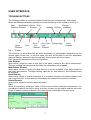
TOOLBAR BUTTONS
The following toolbar is a common feature for all the user environments. This toolbar
allows the different necessary operations for the functioning of the software, see Fig. 2.
New
Modification Delete Print
Element Element
Element
Read
Element
Find
Settings Policies
Go to
Go to Info
First
Last
Element Element
Change
password
Change login
Close
Program
Fig.1 – Toolbar
The elements in the toolbar can be either accessible or inaccessible, depending on the
access rights of the user. In the first case, the user will be able to use the associated
element function, whereas in the second case, this function will not be active.
Here follows the description of the functionalities:
New Element
when active, allows to insert a new line in the table, related to the user’s environment.
Through a dialog that contains all the fields, the information will be added.
Modification Element
when active, allows to modify the data that is in a record, selected in the table related to
the user’s environment. Through a dialog, same as for “new element”, the information will
be modified.
Read Element
when active, allows to read the data that is in a record, selected in the table related to the
user’s environment. In this case the informations are locked and cannot be modified.
Delete Element
when active, allows to cancel a selected record..
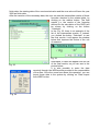
Find
allows the access to a dialog in order to find a record within a selected environment. It is
necessary to specify the field in which you want to carry out the search and the text to be
found. In case of positive response, the cursor will be positioned on the line found.
Fig. 2 – Search dialog
3
Print
allows to print the content of a grid in the selected environment.
Go to First Element
allows the positioning of the cursor on the first record of the grid in the user’s environment.
Go to last Element
allows the positioning of the cursor on the last record of the grid in the user’s environment
Settings
This button is disabled
Info
information related to FlowerTool
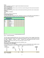
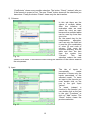
Policies Management
the field that will be proposed at the selection of this icon will enable the administrator to
qualify each “group” of users to the use of the main functions of the program.
Fig. 3 – User Permissions
The first thing the administrator has to do is to select a group to whom assign the policies;
then, by ticking off the boxes, he can authorize the group to carry out certain actions (such
as “Add” – “Modify” – “Cancel” – “Print” – “Search”); he can decide also which of all the
fields should be the first view when the user logs-in (column “First”).
Change Login
allows to use the software with the profile of another user.
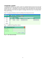
Description of the StatusBar
As the toolbar, also the StatusBar is present in all the environments and supplies some
important informations, such as current user’s environment and current user.
Current
Environment
Time
Date
CAPS
lock
Fig. 4 – Statusbar
4
USER
BASIC OPERATIONS
LOGIN
The first thing to do after starting the program, by using the icon on the desktop, is to add
the following information
•
Server name
1. This is the name of the server where the database is installed. This field is
not editable
•
Login
1. This is the name with which a user is identified (user-ID) within the
FlowerTool; it will be the care of the managers to communicate the user-id’s
for the various users.
2. After the first access, it will not be necessary anymore to digit this ID each
time, unless you want to login with another ID than the last one you used.
•
Password
1. The FlowerTool system administrator will assign temporary passwords for
each user; this password can be changed in another personal one, after the
first access.
2. If you digit a wrong password, the system will give a message (Fig. 6), and
will not allow access until the password is valid.
3. In case you do not remember your password, you should contact the
FlowerTool system administrator, who will supply you with a new one.
Fig. 5 User Login
Note
The default User Name is FlowerTool with password = Tredegar (be careful to the letter in
upper case). This user has right of administrator and then he can create new groups and
new users. Please read the paragraph “Area of Tables” / Users
Fig. 6 Wrong Password
5
PASSWORD CHANGE
To change the password, you need to select the “Change Password” button from the main
toolbar (see Fig. 7). The dialog box (see Fig. 8) asks for the new password in the first field,
and then also for a confirmation in the second field. If these two match, the new password
will be registered. If not, there will appear a message that informs you of a wrong match.
Then you can retry.
Note: The passwords always need to be different from the previous ones.
Fig. 7 – Password Change Menu Option
Fig. 8 – New Password Mask
6
FLOWER TOOL
The Flower Tool program has been designed and implemented to provide a power tool to
evaluate the eco-efficiency index of the companies.
The criteria used to implement the analysis are not explained in this
manual; in fact here you can find the explanation of how to use the
program in order to obtain their results from the analysis.
First of all we describe the Tables Area:
TABLES AREA
Here you can manage all the informations that turn around the ‘kernel’
of the program and that you need to get your analysis.
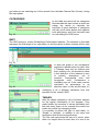
USERS
This environment will propose a table containing the informations
related to the various users that work
with the software.
The users that belong to the group of
administrators can add, modify and
eliminate the users, by clicking on the
related icons on the toolbar.
Each user can be equipped with a
User Name and an access password
and has to be associated to a group
with rights to access and to use the
functions, different from others. The
status of each user can be either
Fig 10 – User mask
active or not: when he is active he will
be present in the combo box, which you will find in the dialog of adding
the users, on the contrary he will not be present if he is not active.
This solution has been adopted in order to avoid that in a list you may
see users who are not involved anymore with the management of the
Fig. 9 – List bar production process or who are not present anymore in the site for
different reasons.
As a matter of fact, the “physical” cancelling of names is not possible if they were present
in some other section. Each user has to be associated with an e-mail address, where he
can be reached for any communication, by electronic mail.
7
USER GROUP
Also in this area we will have a table that
summarizes the groups of users created for
FlowerTool. The users who belong to the
group of administrators can add, modify
and cancel the groups, using the special
buttons on the toolbar. Policies can be
Fig. 11
created for each group, by using “Policies”
button from the toolbar. The administrators
can link each new user to one of the created groups, so that the new user will
automatically inherit the policies defined for the group.
NATIONS
In this table are stored all the nations
involved in some supply (energy, raw
material etc). These informations are useful
to define the coefficients related, precisely,
to the nations.
Fig. 12
MODELS
In this table are stored the names of the data input models that we’ll create afterwards. It’s
possible to create how many models we want and, naming them conveniently, it will be
easy to compose and identify the data input
models of the plants. Anyway you can find
more clarifications in the Voices-Model
Association paragraph. The option buttons
TLEE/TGEE and TPEE allow to specify for
which kind of analysis the model will be
used.
Fig. 13
PLANTS
In this table are stored all the plants for
which we have to evaluate and/or compare
the eco-efficiency.
Of course you have to specify also the
nation for the plant. You can do it by
selecting the nation from the combo box
“Nations”. If the needed nation doesn’t exist
in the list, you can add it pressing the
button with cross icon to the right of the
combo box
Fig. 14
8
UNIT OF MEASURE
In this table are stored all the units of
measure used for representing the
quantities
Fig. 15
VOICES
This table introduce us to one of the
most important concept of the logical
structure of the program. In fact the
voices constitute the fulcrum on which
the program goes around.
They
represent
the
variables
necessary to build the formulas that
give out the intermediate results (or
final results) of the analysis in
consideration.
The enabled users of the plants can
enter such inputs locally, by VB client
program, or remotely, by WEB based
module.
Fig. 16
Fig. 17
For the voices it’s possible to specify a description, a code, an unit of measure and a
category. With the term category we intend one of the codified elements in related
‘Categories’ table, precisely. The checkbox ‘Active’ can be checked off or not. In the first
case the voice is really used inside of still valid formulas. In the second case the voice is
considered not active or, to say better, not used anymore.
Due to reasons of referential integrity, an unused voice will be highlighted in red color (see
Fig. 17) if it is contained in some formulas. That inform us about the obsolescence of the
voice.
The voices can be defined as input type "Normal" or "Variable".
In the first case the user will have to enter a simple cell with a numeric value. In the
second case the choice will be done from a combo box.
In that way the voices will ‘inherit’ the numeric value associated to the field of the related
table, specified during the definition of the voice.
For exemple, as you can see in the Fig. 16, we defined the voice # 161, with code ‘CNG’,
category ‘Natural Gas’ and type of input ‘Variable’. The numeric value will be automatically
9
got when we are selecting one of the records from the table ‘Natural Gas Country’ during
the input phase.
CATEGORIES
In this table are stored all the categories
that describe the input voices at which we
assign the values to calculate the
formulas. A good definition of categories
will help us to better define and organize
both preliminary and final formulas used
for calculating the GPKI index.
Fig. 18
GKPI
The GKPI acronym, means Global Keys Performance Indicator. The elements in this table
represent the final target of our calculation. In fact the values of these indexes will be used
Fig. 19
to draw the graph of the comparative
analysis for period and/or for plant. Also
if Tredegar uses only six indexes and
their quantity is fix, we decided to allow
a free definition of the indexes in term
of quantity, description, unit of
measure, background color and
foreground color. Furthermore a
checkbox says us, if the index must be
calculated as percentage or as
absolute value. In the second case, it’s
Fig. 20
necessary to do a different calculation from that
provided for the ‘normal’ GKPI .
TABLES
Fig. 21
Also the tables represent a very important element
for the logical functionality of the program. They
make flexible the insertion of values selectable from
lists with many items, as for example the combo box
inside the module for managing inputs.
It is possible to define the type of each table, i.e.
‘Simple’ or ‘Multiple’, in addition to his name and
description (that should be significative).
The first case represents the case of a vector, when
there is a single value for each item of a row of the
10
table.
The second case, instead, represents the case of a matrix, when to one row correspond
more values.
The usage with voices at variable values selectable from simple tables, has been already
described; now let’s give a look to understand what you have to do in case of tables with
multiple values:
First of all we say that the grid “Table Details” represents the rows of the matrix whereas
the grid “Table Values” represents the
columns. Clicking on the button with the
green cross in the area “Detail Table”,
you can enter a new “row” for the matrix.
As you can see in the Fig.22 you can
enter a field name and a description for it.
Clicking, instead, on the near button with
Fig. 22
red cross you can delete the selected row
from the area “Detail Table”.
Clicking on the button with the green
cross in the area “Values Table”, you can
enter a new value for the row. As you can
see in the Fig. 23 you can enter a value,
a code, a column name and, above all, a
start date of validity. Clicking, instead, on
the near button with red cross you can
delete the selected row.
The validity date concept is very very
Fig. 23
important, because it allows to update the
values for the coefficients without change the previous analysis made using the old values.
Once defined that matrix, it will be possible to associate this new table to a voice declared
of type “variable”. Anyway more explanations will be provided when we will talk about the
formula’s builder.
CALCULATION AREA
In this environment it’s possible to
manage the formulas used in the
program in order to evaluate the
indicators of the performance.
First of all we see how the form of
the builder has been organized:
CALCULATE LEVEL 1
The text boxes up to the left allow
us to define a code and a
description for the formula. The
choice
of
the
model
is
fundamental because it allows us
to consider the list of the input
voices associated previously to
the model itself.
For example it’s possible to create
a model (Plastic Films) for all the
plants of Tredegar that are
Fig. 24
11
producing plastic films in the world, associate to it a serie of voices of the categories of
environmental impact and use them for the analysis of the plants (how we’ll see better
ahead).
If we want to analyze the eco-efficiency of the plants that are producing films of aluminium,
we can create a new model (Aluminium Films) with different input voices and use them for
the analysis of this other kind of product.
The check box “View among the intermediate results” allows us to specify if we want to
see the result of the formula we are building, or not.
The tabs allow us to select the operands of the formula; they can be, precisely,
Coefficients, Columns, Inputs and Polynomial expressions (Level 1, Level 2, Level 3).
The hierarchical organization of these tabs makes always possible to see and then use
the coefficients, the columns and the inputs, while the levels, instead, are usable only
from higher down to the lower. In fact the level 2 can see the level 1 but it can’t see the
level 3 and so on.
The grid "Functions" allows to select the functions we need to build our formula, from a
long (but not exaustive) list.
The frame “Symbolic Formula” shows the formula represented with the symbols
associated to the operands.
The frame “Decoded Formula” shows the same formula represented with codes and
symbols necessary to the interpreter of the program to decode and evaluate them.
The field "Notes" allows to enter possible notes to the formula
The frame ‘Operators’ allows to insert in the formula the algebric operators
The frame ‘Numbers’ allows to insert in the formula the numeric values
Now we will do some considerations about the Tabs:
1) Coefficients
In this tab there are the
values of simple tables.
After the selection of our
table, we have the combo
box "Field" where we can
choose the field of the table
we want to use . After the
field selection, the value of
the coefficient is shown in
the frame and it is not
editable.
Such coefficient can be
finally used in the formula
we are building clicking on
the “Add” button. The
“Reset” button in the tab
Fig. 25
12
“Coefficients” clears every possible selection. The button “Check”, instead, tells you
if the formula is correct or not. The near “Reset” button clears all the selections you
have done. Finally the button “Delete” clears only the last insertion.
2) Columns
In this tab there are the
values of multiple tables.
After the insertion of
evaluation date, we must
select the voice we want
because the multiple tables
can be used by more than
one voice.
So, the search key for the
interpretation
algorythm,
can’t use only the code, but
it must be the combination
of voice ID and code of
column. That must be
choosed selecting first the
table and then the item
from the combo box
“Column”.
This
last
Fig. 26
selection makes the code
visible in the frame. A convenient control during the insertion of the column ensures
the uniqueness.
3) Input
The tab of inputs is
conceptually
easier
because it shows only the
inputs associated to the
selected model. To insert
an input in the formula you
must double click on the
row in the grid “Input
Values”.
To insert, instead, a
function in the formula, you
can double click on the row
in the grid “Functions” or
click on “Add” button. The
“Reset” button clears the
previous selection.
Fig. 27
13
4) Level 1
In the tab Level 1 there are all the intermediate formulas created for it
5) Level 2
In the tab Level 2 there are all the intermediate formulas created for it
6) Level 3
In the tab Level 3 there are all the intermediate formulas created for it
Theoretically it would been enough only one level of calculation. In fact it is possible to
build also very complex formulas with only one level, but we preferred to divide the
formulas in more levels to make the reading easier and to allow intermediate calculation.
Anyway we don't have introduced any limitations nor imposed strict rules. In fact there are
some indicators that can be composed only by inputs without the need to belong to
intermediate formulas. So, it is possible to avoid doing all the passages up to level 3,
defining them directly in one of the provided levels but, for coherence, we suggest to
declare them always in the same level. This allows to apply always the same scheme and
avoids to understand why sometimes we did in a certain way and some other in a different
way.
For example we defined “Outputs” always at level 3.
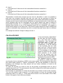
CALCULATE GKPI
In the environment "Calculation”
we find also the GKPI function.
For it we must give a deeply
explanation. The calculation of
normalized GKPI is, really, the
final goal of the program and,
consequently, of all the settings
of the formulas that we have
seen until now. There are some
things we have to notice: first of
all it is necessary to specify the
model for which we are creating
these formulas. In the combo
box will be present only the
plants for which we still have not
created the formulas for GKPI
Fig. 28
This happens because it makes
no sense to create more than
one formula for the calculation of GKPI for the same model. The indicators are taken from
the relative table present in “Tables” environment. We left this possibility to avoid any
limitations, but Tredegar very likely doesn’t will use further indicators, at least for the
plastic films sector.
To insert the formula you need to click on the symbol of percentage both for unit of
measure kg and for m². The environment that will be called will be the same provided for
the levels discussed previously.
Unfortunately it’s impossible to modify the formulas (as for those of other levels, anyway).
You can only delete it and re-create it. It’s also possible to insert the formulas for the
production, both in m² and in t. These data will be shown in the same table of the GKPI,
inside of the graph of eco-efficiency analysis.
14
“MANAGEMENT” AREA
MODELS – VOICES ASSOCIATION
As we saw in the previous paragraphs, it is necessary to make an association among the
input models created before and the defined voices.
Fig. 29
In fact the program provides the possibility to realize eco-efficiency analysis for categories
not always homogeneous. For example, Tredegar produces plastic films with a group of
plants and aluminium films with another group of plants. The eco-efficiency study for these
two kinds of product is based on different inputs and voices. By defining different models
and voices and by creating the convenient associations among them it is possible to
realize the analysis for both the plants that are producing plastic films and those that are
producing aluminium films.
As we can see in the Fig. 29, to create the association, first of all we must create the
model and then we must check off the interested voices. They are shown inside of the tabs
representing respectively the categories defined in the related table.
When we try to modify an association in which there are some voices already used to
create some formulas, the program highlights in red color such voices and it doesn’t allow
their modifying. Those still not used, instead, are not highlighted and they are selectable
regularly.
15
ANALYSIS
Fig. 30
This environment allows to create
an eco-efficiency analysis using the
input voices and, of course, the
formulas provided for selected
model. This involves, precisely, the
selection of the model, the setting of
evaluation date, the selection of the
plant that is subject to the analysis
and the insertion of a description
that identify the analysis itself .
The selection of the model
determines the loading of all the
voices related to it.
The user has to insert the numeric
values in the text box fields and the
selection of a value in the combo
box fields.
The values returned from items
selection in the combo box depend
on the set evaluation date.
This happens because the values
Fig. 31
defined in the single and multiple
tables have a validity period. But if
there are no coefficients or values for the period under consideration, the program will ask
you to insert them manually. The new inserted value, will be the current one, starting from
inserting date, up to year 3000 (to indicate an undefined time). This value will become
outdated when somebody will insert a new value. In fact the previous one will have, as
16
finish date, the starting date of the new inserted value and the new value will have the year
3000 as finish date.
After the insertion of the necessary data, the user can see the intermediate results of those
formulas checked in the related table, by
clicking on the relative button. The final
results (i.e. the results of the formulas
defined for the calculation of the GKPI) will
be shown by clicking on the button
“Calculate”.
In the Fig. 32, there is an example of the
list of the intermediate results. If, instead,
you clicked the button “Calculate” to see
the final results, it will appear the window
below that imposes the choice of the unit
of measure.
Fig. 33
Fig. 32
Afterwards, a frame will appear with the list
of the final results, as you can see in the
picture below.
It is also possible to enter the data
remotely through the WEB module provided to the responsibles
of the sites. Once the users have done this operation, you can
import those data in the system by clicking on “Data Import
from WEB” button.
Fig. 34
17
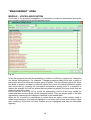
ECO-EFFICIENCY
This environment allows us to realize many comparative analysis of eco-efficiency . Here it
is possible to compare analysis and group them as an eco-efficiency study. The example
Fig. 35
in the Fig. 35 shows us the main grid (2010 – Analysis – Europe Plants) and related
details.
The insertion of a new study involves also the insertion of the referring year and of an
appropriate description.
The frame “Filter Analysis” has just the
function to show all the analysis in the
grid “Analysis List” for a given period
and plant. The selection of the analysis
must be done based on the type of
comparison that we want to do. For this
reason it’s better to give a significative
name to the eco-efficiency studies.
To continue the previous example, we
considered a study called “2009 –
Analysis Europe Plants” because we
would compare the analysis of 2009 for
the european plants, conveniently
created inside of the analysis
environment.
In this case we must tick off the check
box of “TLEE Roccamontepiano”,
“TLEE Kerkrade 2009” and "TLEE
Retsag 2009”.
Be careful because if we now choose
also “San Paolo” we haven’t any ways
to notice the mistake, but we can
understand that there is something
wrong only observing the final results.
Fig. 36
This feature represent an advantage of
the program (in terms of flexibility) but
in the same time it is a small limitation of its rigorousness.
It is possible to open a saved study of eco-efficiency to get a graph for it.
18
By re-opening the study it will be possible to click on the button “Calculate”. The first
information we must enter is the unit of measure. After waiting for the computing time,
subject to the number of the analysis we are considering and to the hardware in use, the
form will appear. It will be divided in some tabs, one for each analysis. Each tab,
Fig. 36
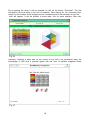
precisely, contains a table with all the values of the GKPI, the production data, the
percentage of LEE and a peculiar graph with the form of stylized exagonal flower
Fig. 37
19
representing the basic analysis of the study.
Clicking on the button “Export” we get a comparative graph as in the Fig. 37. In its columns
are represented the numeric values of tables present in each tab, respectively, and the
thumbnail of the related graph.
It’s possible to print this graph by clicking on “Print” button.
TLEE-TGEE
This environment allows us to compare the eco-efficiency analysis we have done, in order
to obtain two kinds of different graphs, TLEE and TGEE.
The TLEE compares the eco-efficiency studies in a selected period.
If you need you can print the page by clicking “Print” button.
Fig. 38
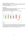
The TGEE, instead, represents the normalized calculation of the GKPI indicators of all the
eco-efficiency analysis. It is composed by two pages: the first shows a table containing
numeric values and a thumbnail of the flower-graph, while the seconds shows a bar graph.
Each bar represents one column of the table in the first page. If you need you can print the
page by clicking “Print” button. Click, instead, arrows buttons to navigate.
20
Fig. 39
Fig. 40
21
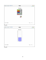
TPEE
The TPEE is the evaluation of the difference among the eco-efficiency studies, related to a
specific project. The user can focus on a study and compare it with the others, in order to
calculate the deviation (see “Delta TPEE” in Fig. 41). The page is composed by four main
elements:
- a table with the numeric values of the GKPI indicators for each project
- the thumbnail of the flower-chart for each project
- a bar-chart with a bar for each eco-efficiency value of the project
- a table with the TPEE deviation ("Delta TPEE")
Fig. 41
If you need you can print the page by clicking “Print” button. The “Settings” button, instead,
allows you to enter manually the “Weight Factors”, i.e. the importance of the GKPI
indicators within the flower-chart. Furthermore you can specify if the study is “PEIA
NATURAL” or not.
Fig. 42
22