Download pdf, 2 MiB - Infoscience

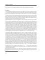
Distributed Sensor Data Models and Their Impact on Energy
Consumption of Wireless Sensor Networks
THÈSE NO 5364 (2013)
PRÉSENTÉE le 18 février 2013
À LA FACULTÉ INFORMATIQUE ET COMMUNICATIONS
LABORATOIRE DE SYSTÈMES D'INFORMATION RÉPARTIS
PROGRAMME DOCTORAL EN INFORMATIQUE, COMMUNICATIONS ET INFORMATION
ÉCOLE POLYTECHNIQUE FÉDÉRALE DE LAUSANNE
POUR L'OBTENTION DU GRADE DE DOCTEUR ÈS SCIENCES
PAR
Urs Hunkeler
acceptée sur proposition du jury:
Prof. M. Grossglauser, président du jury
Prof. K. Aberer, Dr P. Scotton, directeurs de thèse
Dr J. Beutel, rapporteur
Dr P. R. Chevillat, rapporteur
Prof. P. J. M. Havinga, rapporteur
Suisse
2013
I didn’t know it was impossible
when I did it.
— Source Unknown
To my family and my wife.
Acknowledgements
This thesis was made possible with the support of the IBM Research GmbH in Rüschlikon and
I would like to express my thanks to IBM for investing in young researchers.
Prof. Dr. Karl Aberer, thank you for your inspiration and support. I appreciate that with all
your commitments you always found the time to see me when I asked for a meeting.
Dr. Paolo Scotton, thank you for all the help and advice that you have given me. I particularly
appreciate your management style and your fresh views on challenges.
I would like to express my special thanks to my thesis committee. You all inspired my work at
different stages, and I am very glad that you all accepted to be in this committee. I appreciate
that you read my work carefully and I thank you for the detailed and constructive comments.
Many people have helped and supported me at EPFL, and it would be difficult to mention
you all. Dr. Catherine Dehollain, thank you for a great opportunity and an interesting research topic. Special thanks go to Chantal François and Isabelle Buzzi for their help with all
the administrative details and to the IT support for the creative ideas on how to deal with
unconventional problems.
The IBM Zurich Research Laboratory (ZRL) is a welcoming place for researchers and I made
many friends. Therefore I have to ask you to forgive me for not mentioning everyone individually. I would like to thank the present and former ZRL employees who made IBM a fun place
to work and who organized or participated in the many social events. In particular I would
like to thank Dr. Hong Linh Truong, Beat Weiss, and Dr. Clemens Lombriser for all their help. I
would also like to thank Tomas Tuma for his friendship and the memorable hikes.
Thank you, Dr. James Colli-Vignarelli and José Demétrio, for all your help and your patience
when I was stressed.
Special Thanks go to Diego Wyler who made me aware of the communication systems section
at EPFL. Because of Diego’s recommendation I decided to study communication systems at
EPFL and the Institut Eurécom, and after all these years it is clear that it was exactly the right
decision.
I am very grateful to my parents for their support and encouragement from an early age on.
Thank you for kindling my curiosity already as a small child and for always giving me honest
answers. Thank you for your patience. Thank you also to Charlotte and Roli for your support
and understanding, and I wish you all the best for your studies.
Dr. Fereshteh Bagherimiyab-Hunkeler, you appeared as my angel when I needed you. Thank
you so much for completing my life and for accepting me the way I am. I love you.
Thank you to all of you who have helped me during my thesis and who I could not mention
v
Acknowledgements
individually.
Lausanne, January 18, 2013
vi
Abstract
Electronic hardware continues to get "smarter" and smaller. One side-effect of this development is the miniaturization of sensors, and in particular the emergence of battery-operated,
multi-hop wireless sensor networks (WSN). WSNs are already used in a wide variety of different
applications, ranging from climate monitoring to process compliance enforcement.
Ideally, WSN hardware should be small, cheap, multi-functional, autonomous and low-power
(thus battery-operated), and the network should be self-configurable. To satisfy the low-power
requirement, nodes are typically able to communicate only over a short distance and rely on
multi-hop for longer range communication.
Wireless sensor networks promise to monitor objects and areas at an unprecedented level of
detail. Such observations result in large amounts of data that cannot be analyzed manually.
Instead, algorithms are used to summarize the data into meaningful measures or to detect
unexpected or critical situations.
The main challenge for WSNs today is the power consumption of the individual devices, and
thus the lifetime of the overall network. Most energy is used for communication. As WSN
nodes do not simply transmit raw sensor readings but have the capability to process data, it is
natural to look into preprocessing the data already inside the network in order to reduce the
amount of data that needs to be transmitted.
In this thesis we study the possibilities and effects of in-network data processing. Our approach
differs from previous work in that we look at the system as a whole. We look at the processing
algorithms that would be performed on the data anyway and try to use them to reduce the
amount of data transmitted in the network. We study the effects of various data reduction
approaches on the power consumption. Our observations and conclusions enable us to
propose a framework to automatically generate and optimize code for running on distributed
WSN hardware based on a description of the overall processing algorithms.
Our main findings are that (1) the energy-saving potential of algorithms need to be validated
by taking into account the whole system – including the hardware layer, that (2) the most
efficient data-reduction algorithms only process data produced by the sensor node on which
the algorithm is running, and that (3) efficient in-network processing code can be generated
only based on an overall description of the processing to be performed on data.
Our main contributions to the state-of-the-art are (1) a general-purpose framework for automatically generating sensor data processing code to run in a distributed fashion inside the
WSN, including a data processing language and a meta-compiler, (2) an extension of the WSN
hardware simulator Avrora that makes it truly multi-platform capable, and (3) a centrally
vii
Abstract
managed, low-power, multi-hop WSN system (IMPERIA), which is now used commercially.
We start this thesis with a presentation of the related work and of the background information
to understand the context of WSNs and model processing. We then present approaches for
distributed model processing, we propose a framework to generate and optimize distributed
model processing code, we present our implementation of the framework and in particular of
the compiler, we present our measurement setup and our measurement results, and finally
we present a commercial WSN system based on the concepts and expertise presented in this
thesis.
Keywords: Wireless Sensor Network, energy efficiency, sensor data model, distributed processing, automatic generation of distributed code, TinyOS, IMPERIA
viii
Zusammenfassung
Elektronische Geräte werden immer ïntelligenteründ kleiner. Ein Nebeneffekt dieser Entwicklung ist die Miniaturisierung von Sensoren, und speziell die Entwicklung von batteriebetriebenen, kabellosen Sensornetzwerken (wireless sensor networks, WSN) mit Datenweiterleitung.
WSNs werden bereits für eine breite Auswahl von verschiedenen Anwendungen eingesetzt,
von Klimaüberwachung bis Prozess-Konformitätssicherung.
WSN Geräte sollten idealerweise klein, kostengünstig, vielseitig einsetzbar, eigenständig und
energiesparend (daher batteriebetrieben) sein, und das Netzwerk sollte sich selbständig konfigurieren. Um Energiesparsamkeit zu ermöglichen, können Knoten üblicherweise nur über
kurze Distanzen direkt kommunizieren und verlassen sich auf Datenweiterleitung für längere
Verbindungen.
Kabellose Sensornetzwerke versprechen, Objekte und Gebiete mit einer beispiellosen Genauigkeit zu überwachen. Solche Überwachungen erzeugen grosse Mengen an Daten, welche
nicht manuell ausgewertet werden können. Daher werden Algorithmen verwendet, welche die
Daten in nützlichen Grössen zusammenfassen oder automatisch heikle Situationen erkennen.
Die wichtigste Herausforderung für WSNs ist heute der Energieverbrauch der einzelnen Geräte,
und daher auch die Lebenszeit des gesamten Netzwerkes. Die meiste Energie wird für die
Datenübertragung verwendet. Da WSN Knoten nicht einfach nur rohe Sensormessungen
übermitteln, sondern auch die Möglichkeit haben, Daten zu verarbeiten, ist es natürlich zu
versuchen, die Daten bereits im Netzwerk vorzuverarbeiten um die Menge der Daten, welche
übermittelt werden müssen, zu reduzieren.
In dieser Doktorarbeit untersuchen wir die Möglichkeiten und Wirkungen der Datenverarbeitung im Netzwerk. Unser Ansatz unterscheidet sich von früheren Arbeiten darin, dass wir das
System als ganzes betrachten. Wir untersuchen die Datenverarbeitungsalgorithmen, welche
so oder so auf die Daten angewendet würden, und versuchen, sie zum Reduzieren der zu
übermittelnden Daten zu verwenden. Wir untersuchen die Wirkung verschiedener Datenreduzierungsansätze auf den Energieverbrauch. Unsere Beobachtungen und Schlussfolgerungen
ermöglichen es uns, ein Rahmenverfahren vorzuschlagen, um Programmcode, basierend auf
der Beschreibung des gesamten Datenverarbeitungsalgorithmus, für das Berechnen in einem
verteilten WSN automatisch zu generieren und zu optimieren.
Unsere wichtigsten Erkenntnisse sind, dass (1) das Energiesparpotenzial eines Algorithmus
unter Berücksichtigung des gesamten Systems bewertet werden muss – die Hardwareschicht
inbegriffen, dass (2) die effizientesten Datenreduzierungsalgorithmen nur Daten vom Sensorknoten, auf dem die Berechnung läuft, verwenden, und dass (3) effiziente Datenverarbeitung
ix
Abstract
im Netzwerk nur basierend auf der gesamten Beschreibung der Datenverarbeitung, welche
auf die Daten angewendet werden soll, generiert werden kann.
Unsere wichtigsten Beiträge zum Stand der Technik sind (1) ein generisches Rahmenverfahren,
um automatisch Code für die verteilte Verarbeitung von Sensordaten in einem WSN zu generieren, einbezüglich einer Datenverarbeitungssprache und einem Meta-Compiler, (2) eine
Erweiterung des Simulators von WSN Geräten Avrora, welche es diesem Simulator zum ersten
Mal wirklich ermöglicht, mehrere Plattformen zu unterstützen, und (3) ein zentral verwaltetes,
energiesparendes, Daten weiterleitendes WSN Systems (IMPERIA), welches nun kommerziell
verwendet wird.
Wir beginnen diese Doktorarbeit mit einer Präsentation von verwandten Arbeiten und von
Hintergrundinformationen bezüglich kabellose Sensornetzwerke und Datenmodellierung.
Wir stellen dann Ansätze für das verteilte Verarbeiten von Datenmodellen vor, wir schlagen
ein Rahmenverfahren für die Generierung und Optimierung von verteilten Algorithmen für
Datenmodellierung vor, wir präsentieren unsere Umsetzung des Rahmenverfahrens, und insbesondere des Compilers, wir erläutern unsere Messeinrichtung und unsere Messergebnisse,
und schliesslich beschreiben wir ein kommerzielles WSN System, welches auf den Konzepten
und Erfahrungen dieser Doktorarbeit beruht.
Stichworte: Kabellose Sensornetzwerke, Energieeffizienz, Sensordatenmodell, verteilte Verarbeitung, automatisches Generieren von verteilten Programmen, TinyOS, IMPERIA
x
Contents
Acknowledgements
Abstract (English/Deutsch)
v
vii
List of figures
xiii
List of tables
xv
1 Introduction
1
2 Related Work
7
2.1 Introduction . . . . . . . . . . . . . . . . . . . . . . . . . . . . . . . . . . . . . . . .
7
2.2 State of the Art . . . . . . . . . . . . . . . . . . . . . . . . . . . . . . . . . . . . . . .
7
2.3 Wireless Networking Approaches . . . . . . . . . . . . . . . . . . . . . . . . . . . .
9
2.3.1 WiFi . . . . . . . . . . . . . . . . . . . . . . . . . . . . . . . . . . . . . . . . .
9
2.3.2 Bluetooth . . . . . . . . . . . . . . . . . . . . . . . . . . . . . . . . . . . . .
9
2.3.3 Wireless Mesh Network . . . . . . . . . . . . . . . . . . . . . . . . . . . . .
9
2.3.4 Mobile Ad-hoc Networks . . . . . . . . . . . . . . . . . . . . . . . . . . . .
9
2.3.5 Wireless Sensor Networks . . . . . . . . . . . . . . . . . . . . . . . . . . . .
10
2.4 Device Categories for WSNs . . . . . . . . . . . . . . . . . . . . . . . . . . . . . . .
10
2.4.1 Radio-frequency Identification . . . . . . . . . . . . . . . . . . . . . . . . .
11
2.4.2 Mote-class WSNs . . . . . . . . . . . . . . . . . . . . . . . . . . . . . . . . .
11
2.4.3 PDA-class WSNs . . . . . . . . . . . . . . . . . . . . . . . . . . . . . . . . .
11
2.4.4 Laptops . . . . . . . . . . . . . . . . . . . . . . . . . . . . . . . . . . . . . . .
11
2.4.5 Conclusion . . . . . . . . . . . . . . . . . . . . . . . . . . . . . . . . . . . . .
12
2.5 Hardware Devices for Mote-class Sensor Networks . . . . . . . . . . . . . . . . .
12
2.6 MAC Layer . . . . . . . . . . . . . . . . . . . . . . . . . . . . . . . . . . . . . . . . .
15
2.7 Routing . . . . . . . . . . . . . . . . . . . . . . . . . . . . . . . . . . . . . . . . . . .
18
2.8 Transport Layer / Middleware . . . . . . . . . . . . . . . . . . . . . . . . . . . . . .
18
2.8.1 Publish/Subscribe . . . . . . . . . . . . . . . . . . . . . . . . . . . . . . . .
19
2.9 Aggregation / Compression . . . . . . . . . . . . . . . . . . . . . . . . . . . . . . .
20
2.9.1 Problems of Distributed Aggregation . . . . . . . . . . . . . . . . . . . . .
21
2.9.2 Common Aggregation Operators . . . . . . . . . . . . . . . . . . . . . . . .
22
2.10 Simulating Energy Consumption . . . . . . . . . . . . . . . . . . . . . . . . . . . .
25
xi
Contents
2.11 Conclusion . . . . . . . . . . . . . . . . . . . . . . . . . . . . . . . . . . . . . . . . .
3 Sensor Data Models
29
3.1 Introduction . . . . . . . . . . . . . . . . . . . . . . . . . . . . . . . . . . . . . . . .
29
3.2 Deterministic Models . . . . . . . . . . . . . . . . . . . . . . . . . . . . . . . . . .
32
3.3 Linear Regression . . . . . . . . . . . . . . . . . . . . . . . . . . . . . . . . . . . . .
35
3.4 Multivariate Gaussian Random Variables . . . . . . . . . . . . . . . . . . . . . . .
39
3.5 Practical Model: Vibration Sensing . . . . . . . . . . . . . . . . . . . . . . . . . . .
40
3.6 Conclusion . . . . . . . . . . . . . . . . . . . . . . . . . . . . . . . . . . . . . . . . .
41
4 Framework
43
4.1 Introduction . . . . . . . . . . . . . . . . . . . . . . . . . . . . . . . . . . . . . . . .
43
4.2 Framework for Distributed Sensor Data Models . . . . . . . . . . . . . . . . . . .
43
4.3 Model Description Language . . . . . . . . . . . . . . . . . . . . . . . . . . . . . .
46
4.3.1 Linear Regression . . . . . . . . . . . . . . . . . . . . . . . . . . . . . . . . .
49
4.3.2 Multivariate Gaussian Random Variables . . . . . . . . . . . . . . . . . . .
50
4.3.3 Wind-flow Model . . . . . . . . . . . . . . . . . . . . . . . . . . . . . . . . .
51
4.3.4 Vibration Sensing . . . . . . . . . . . . . . . . . . . . . . . . . . . . . . . . .
54
4.4 Execution Environment . . . . . . . . . . . . . . . . . . . . . . . . . . . . . . . . .
54
4.5 Conclusion . . . . . . . . . . . . . . . . . . . . . . . . . . . . . . . . . . . . . . . . .
56
5 Compiler
59
5.1 Introduction . . . . . . . . . . . . . . . . . . . . . . . . . . . . . . . . . . . . . . . .
59
5.2 Implementation of the Compiler . . . . . . . . . . . . . . . . . . . . . . . . . . . .
59
5.2.1 Modular Compiler Design . . . . . . . . . . . . . . . . . . . . . . . . . . . .
60
5.2.2 Parser / Lexer . . . . . . . . . . . . . . . . . . . . . . . . . . . . . . . . . . .
62
5.2.3 Enhanced AST . . . . . . . . . . . . . . . . . . . . . . . . . . . . . . . . . . .
62
5.2.4 Optimization Modules . . . . . . . . . . . . . . . . . . . . . . . . . . . . . .
63
5.2.5 Cost Function . . . . . . . . . . . . . . . . . . . . . . . . . . . . . . . . . . .
67
5.2.6 Code Generation . . . . . . . . . . . . . . . . . . . . . . . . . . . . . . . . .
68
5.3 Compiling the Models . . . . . . . . . . . . . . . . . . . . . . . . . . . . . . . . . .
68
5.3.1 Linear Regression as Example with Details . . . . . . . . . . . . . . . . . .
68
5.3.2 Multivariate Gaussian Random Variables . . . . . . . . . . . . . . . . . . .
71
5.3.3 Wind-flow Model . . . . . . . . . . . . . . . . . . . . . . . . . . . . . . . . .
71
5.3.4 Vibration model . . . . . . . . . . . . . . . . . . . . . . . . . . . . . . . . . .
72
5.4 Implementation of the Execution Environment . . . . . . . . . . . . . . . . . . .
75
5.5 Conclusion . . . . . . . . . . . . . . . . . . . . . . . . . . . . . . . . . . . . . . . . .
76
6 Performance Evaluation
xii
27
77
6.1 Introduction . . . . . . . . . . . . . . . . . . . . . . . . . . . . . . . . . . . . . . . .
77
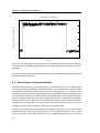
6.2 Measurement Setup . . . . . . . . . . . . . . . . . . . . . . . . . . . . . . . . . . .
77
6.2.1 Sending Data . . . . . . . . . . . . . . . . . . . . . . . . . . . . . . . . . . .
81
6.2.2 Receiving Data . . . . . . . . . . . . . . . . . . . . . . . . . . . . . . . . . .
84
Contents
6.3
6.4
6.5
6.6
6.7
6.8
Network Topology Changes and Management Overhead
Energy Consumption for Data Processing . . . . . . . . .
Measurements Using Soundcards . . . . . . . . . . . . .
Hardware Simulation . . . . . . . . . . . . . . . . . . . . .
Experimental Results . . . . . . . . . . . . . . . . . . . . .
Conclusion . . . . . . . . . . . . . . . . . . . . . . . . . . .
7 Commercial Deployment
7.1 Introduction . . . . . . . . . . . . . .
7.2 Sensor and Network Requirements .
7.3 WSN Design Process . . . . . . . . .
7.4 Hardware Design . . . . . . . . . . .
7.5 Protocol Stack . . . . . . . . . . . . .
7.6 Management Mode . . . . . . . . . .
7.6.1 Network Discovery . . . . . .
7.6.2 Link Probing . . . . . . . . . .
7.6.3 Routing . . . . . . . . . . . . .
7.6.4 Scheduling . . . . . . . . . . .
7.6.5 Configuration . . . . . . . . .
7.6.6 Reusing Configurations . . .
7.6.7 Debugging . . . . . . . . . . .
7.7 Regular Operation Mode . . . . . . .
7.7.1 Reconfiguration . . . . . . . .
7.7.2 Exception Handling . . . . .
7.8 Reference Time . . . . . . . . . . . .
7.9 Conclusion . . . . . . . . . . . . . . .
.
.
.
.
.
.
.
.
.
.
.
.
.
.
.
.
.
.
.
.
.
.
.
.
.
.
.
.
.
.
.
.
.
.
.
.
.
.
.
.
.
.
.
.
.
.
.
.
.
.
.
.
.
.
.
.
.
.
.
.
.
.
.
.
.
.
.
.
.
.
.
.
.
.
.
.
.
.
.
.
.
.
.
.
.
.
.
.
.
.
.
.
.
.
.
.
.
.
.
.
.
.
.
.
.
.
.
.
.
.
.
.
.
.
.
.
.
.
.
.
.
.
.
.
.
.
.
.
.
.
.
.
.
.
.
.
.
.
.
.
.
.
.
.
.
.
.
.
.
.
.
.
.
.
.
.
.
.
.
.
.
.
.
.
.
.
.
.
.
.
.
.
.
.
.
.
.
.
.
.
.
.
.
.
.
.
.
.
.
.
.
.
.
.
.
.
.
.
.
.
.
.
.
.
.
.
.
.
.
.
.
.
.
.
.
.
.
.
.
.
.
.
.
.
.
.
.
.
.
.
.
.
.
.
.
.
.
.
.
.
.
.
.
.
.
.
.
.
.
.
.
.
.
.
.
.
.
.
.
.
.
.
.
.
.
.
.
.
.
.
.
.
.
.
.
.
.
.
.
.
.
.
.
.
.
.
.
.
.
.
.
.
.
.
.
.
.
.
.
.
.
.
.
.
.
.
.
.
.
.
.
.
.
.
.
.
.
.
.
.
.
.
.
.
.
.
.
.
.
.
.
.
.
.
.
.
.
.
.
.
.
.
.
.
.
.
.
.
.
.
.
.
.
.
.
.
.
.
.
.
.
.
.
.
.
.
.
.
.
.
.
.
.
.
.
.
.
.
.
.
.
.
.
.
.
.
.
.
.
.
.
.
.
.
.
.
.
.
.
.
.
.
.
.
.
.
.
.
.
.
.
.
.
.
.
.
.
.
.
.
.
.
.
.
.
.
.
.
.
.
.
.
.
.
.
.
.
.
.
.
.
.
.
.
.
.
.
.
.
.
.
.
.
.
.
.
.
.
.
.
.
.
.
.
.
.
.
.
.
.
.
.
.
.
.
.
.
.
.
.
.
.
.
.
.
.
.
.
.
.
.
.
.
.
.
.
.
.
.
.
.
.
.
.
.
.
.
.
.
.
.
.
.
.
.
.
.
.
.
.
.
.
.
.
.
.
.
.
.
.
.
.
.
.
85
87
88
89
92
94
.
.
.
.
.
.
.
.
.
.
.
.
.
.
.
.
.
.
97
97
98
99
101
102
103
104
105
105
105
108
108
108
109
110
111
112
114
8 Conclusion
117
A Contributions to Publications
119
Bibliography
133
Curriculum Vitae
135
xiii
List of Figures
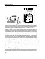
1.1 Different elements of a wireless sensor node. . . . . . . . . . . . . . . . . . . . . .
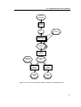
1.2 Typical setup of a WSN. . . . . . . . . . . . . . . . . . . . . . . . . . . . . . . . . .
4
4
3.1 A typical WSN configuration with both a geographical and a corresponding
hierarchical view. . . . . . . . . . . . . . . . . . . . . . . . . . . . . . . . . . . . . .
3.2 Vibration Data Processing. . . . . . . . . . . . . . . . . . . . . . . . . . . . . . . .
39
41
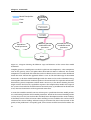
4.1 Different steps and elements of the sensor data model framework. . . . . . . . .
44
5.1 AST of the linear regression model. . . . . . . . . . . . . . . . . . . . . . . . . . .
5.2 Steps in the compilation process. . . . . . . . . . . . . . . . . . . . . . . . . . . . .
5.3 Vibration model data flow. . . . . . . . . . . . . . . . . . . . . . . . . . . . . . . . .
60
61
74
6.1
6.2
6.3
6.4
6.5
6.6
6.7
6.8
78
79
83
86
88
91
93
94
Active circuit for precise power measurements. . . . . . . . . . .
Setup for automatic power measurements. . . . . . . . . . . . . .
Power consumption for sending a single message. . . . . . . . .
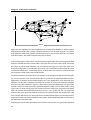
Topology of a WSN deployment in an industrial complex. . . . .
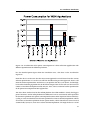
Power consumption of FFT. . . . . . . . . . . . . . . . . . . . . . .
Power consumption of data collection applications. . . . . . . .
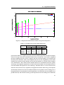
Comparison of the different models. . . . . . . . . . . . . . . . . .
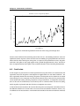
Evolution of prediction error over time using SensorScope data .
.
.
.
.
.
.
.
.
.
.
.
.
.
.
.
.
.
.
.
.
.
.
.
.
.
.
.
.
.
.
.
.
.
.
.
.
.
.
.
.
.
.
.
.
.
.
.
.
.
.
.
.
.
.
.
.
.
.
.
.
.
.
.
.
.
.
.
.
.
.
.
.
xv
List of Tables
2.1 Different classes of wireless networks. . . . . . . . . . . . . . . . . . . . . . . . . .
2.2 Commonly used sensor devices for mote-class WSNs . . . . . . . . . . . . . . . .
10
13
6.1
6.2
6.3
6.4
83
87
92
93
Duration of the different phases of a data transmission. . . . . . . . .
Power consumption comparison for different FFT implementations.
Power consumption data from simulation runs. . . . . . . . . . . . . .
Detailed results of the model comparison. . . . . . . . . . . . . . . . .
.
.
.
.
.
.
.
.
.
.
.
.
.
.
.
.
.
.
.
.
.
.
.
.
xvii
1 Introduction
Electronic devices are an important part of modern life. We use computers, cell-phones, the
Internet, and a variety of specialized devices, either personal gadgets or circuits integrated
into our environment. Lights are automatically turned on when it gets too dark or when a
moving person is detected, and the temperature in our homes is automatically regulated. The
interactions between the real and the virtual worlds are currently still quite limited and usually
restricted to a user’s explicit actions. Most sensors are dedicated to a single purpose and are
hardwired to the electronic device using the data with only a limited interaction with other
sensors or devices.
The reason that sensors are often bound to a single device is the cost for the installation and
the complexity of the configuration of data exchange. With new developments in sensor technology, such as micro-electro-mechanical systems (MEMS), and with advances in electronics
and wireless data communication, general-purpose sensors are emerging. Some electronic
devices, such as laptops and smart-phones, include a series of sensors that are being used
for innovative new applications. For example, many laptops include an accelerometer whose
original purpose is to put the hard-drive into a secure mode when the laptop is being dropped.
This accelerometer is used by games that can be played by moving the laptop around, and the
Quake-Catcher [26] project creates a network of sensors in laptops to detect earthquakes.
The availability of low-cost sensor and communication hardware makes new sensing approaches feasible. An area of interest, such as an industrial installation or a specific geographic
zone, can be monitored at a much greater level of detail and at a lower cost than was previously possible. Battery-operated wireless sensing devices simplify the installation as no
additional wiring is needed. A network of such sensing devices is called a wireless sensor
network (WSN). There are three main application areas for WSNs: (1) home automation, (2)
industrial monitoring, and (3) environmental monitoring.
Home Automation: In a modern home many things can be automated, for instance closing
the blinds when there is too much sun light, controlling the room temperature, automatically turning the lights on, etc. Modular control systems for home automation are
1
Chapter 1. Introduction
commercially available and can be extended by adding additional sensors and actuators.
Similarly, many burglar alarm systems can be extended by adding additional break-in
sensors. To minimize installation costs, these sensors are typically battery operated and
wireless. However, most actuators and the central control module are mains powered
and thus do not need to implement a sophisticated power-management strategy for
their radio interface. The challenges in home automation networks are quite different
from the challenges in the other types of WSNs, and we will not study home automation
networks further in this thesis.
Industrial Monitoring: A modern factory or processing plant is highly automated. Supervising the correct operation and maintaining the machines is thus fundamental to the
operation of industrial sites. WSNs promise to enhance the detail of the supervision of
the installations at reduced cost. The additional information provided by the sensors
can be used to detect failures early, and to optimize maintenance schedules.
The expertise, insight, and some tools developed for this thesis were used to implement
a commercial prototype of an industrial monitoring application. In this context, several
large oil processing plants need to be monitored for vibrations generated by the heavy
machinery, since some of the plants are located near buildings or recently discovered
archaeological sites. The petrol industry’s safety is heavily regulated; installing a wired
network is very expensive and time consuming as the installation needs to be approved
by state agencies and the mounting of the sensors needs to be done by specialists
with state-approved safety training. The expensive procedures of the safety regulations
do not apply to battery-operated devices with very low-power radio emissions; WiFi
networks and cellphones, however, are too powerful and thus are not permitted on
site. A battery-powered multi-hop wireless sensor network is the best approach in this
situation. A battery-powered device using radio communication can be attached to
non-critical equipment or planted in the ground by any plant worker without the need
of government approval. As the permitted transmission power is very low, direct links
are not always possible across the whole area and a multi-hop network is needed. We
provide more details in Chapter 7.
Environmental Monitoring: The classic WSN scenario is environmental monitoring, where
wireless sensors are used to instrument the habitat of animals [112], observe the environment of plants [116], monitor seismic activity [122], detect fires [8], or collect data
for research in hydrology [117]. The different phases of research with WSNs can be explained with a WSN deployment, partially based on a real case [10]. In this deployment,
a mountain village experiences sporadic floods caused by a glacier. Climatologists are
tasked to study the glacier and find a way to predict floods and alert the population.
The scientists install a sensor network to monitor the micro-climate of the glacier by
observing, e.g., the surface temperature of the ice, the duration and intensity of sunshine, the amount of precipitation, and other similar factors. The network operation
can be divided into three stages (the three ‘E’s): (1) exploration, (2) exploitation and
(3) exception. At first, the scientists do not know exactly how the glacier behaves. At
2
this stage, exploration, they use the data from the sensor network to find out how the
different factors influence the state of the glacier. Once the scientists understand the
behavior of the glacier, they can express their knowledge in a mathematical model. The
model might describe how much the ice melts in a variety of weather conditions and
how water accumulates beneath the glacier. It could further describe the conditions that
lead to the ice barrier breaking and releasing the water. In the exploitation stage, this
model of the glacier combined with the current data from the WSN is used to predict
floods. If an unexpected event occurs, that is not properly represented in the model,
the system might fail to properly predict the behavior of the glacier and an impending
flood might go unnoticed. For instance, a dirt avalanche from the hills at the outset
of the glacier could cause the ice to be covered with a small layer of dust. The dust
could completely change the heat absorption rate of the glacier, and thus influence the
amount of water melted on a sunny day. In the exception stage, this model rupture
might be detected when the measured surface temperature of the glacier differs from
the expected surface temperature given the amount of sunshine received by the glacier.
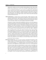
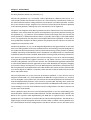
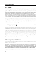
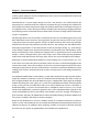
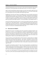
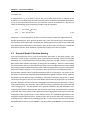
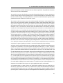
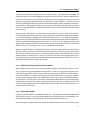
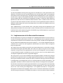
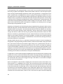
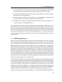
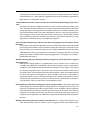
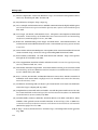
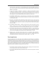
A typical sensor node, as depicted in Figure 1.1, consists of a set of sensors connected to a
microcontroller (µC) which in turn is connected to a low-power radio module. Current devices
are typically powered by batteries. In addition, many deployed sensor nodes try to harvest
energy from the environment, e.g., with solar panels. Because the devices are designed for
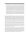
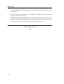
low power consumption, the radio module’s communication range is limited. Maximum
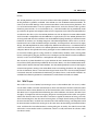
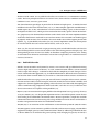
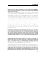
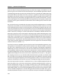
transmission ranges of 20 m indoors and 100 m outdoors are common. To monitor larger areas,
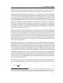
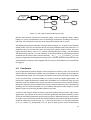
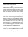
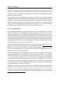
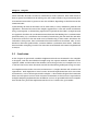
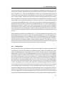
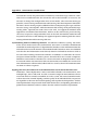
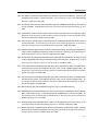
sensor nodes form a network, like the one depicted in Figure 1.2, where nodes relay data from
neighboring nodes and one or more node is directly connected to a gateway (GW) computer
and relays the data through this computer to the back-end system for further processing.
WSNs allow to measure and automatically monitor physical properties over time with high
spatial and temporal resolution. The flip-side is that large amounts of data are available
and need to be processed. To deal with the large amount of data generated by a WSN, it
is necessary to use data models to simplify the analysis of this data. A major difference to
traditional sensing installations is that the sensor devices in a WSN have some processing
capability, the µC in Figure 1.1, and hence data can already be processed, filtered, compressed,
and aggregated on the way to its destination.
Currently, data models are processed on back-end systems. Many data models, especially if
based on complex deterministic models, are computationally expensive and therefore cannot
be processed efficiently on the low-power devices typically used for sensor networks. It is often
possible to do a first part of the processing already within the WSN. In this way, only the data
necessary for the model processing, rather than every single sensor reading, is transmitted.
This helps to reduce the power consumption as well as to resolve bandwidth bottlenecks. In
addition, some data models are able to exploit redundancy in sensor readings to make the
data assimilation of a sensor network more robust to transmission errors [106].
3
0(#$(("
Chapter 1. Introduction
'$()*%)
+,
-"./*
!"##$%&
Figure 1.1: Block diagram of the different elements of a wireless sensor node: Sensors, microcontroller (µC), radio (with antenna), and power source (battery).
&'(
!"#$%"&
!"#$%"$#
Figure 1.2: A typical setup of a WSN: The sensor nodes are connected to the Internet or a
back-end network through a sensor-node-PC pair acting as the gateway (GW).
4
A key concern with battery-powered WSNs is the lifetime of such devices, and by extension
of the sensor network installation. Often, it is not economical to exchange batteries, and
hence the batteries of the devices, and thus the devices themselves, should last for as long
as possible. As an example, a TelosB sensor node with a standard pair of AA-sized batteries
lasts approximately one week if no special power saving measures are implemented and the
µC and radio module remain active the whole time. With proper power management, the
same sensor node with the same type of batteries can last for more than a year while regularly
transmitting sensor readings and relaying readings of other sensors.
Much of the current research on WSNs focuses on how to reduce the energy consumption of
the devices. In most cases the biggest energy consumer is the radio module (see Chapter 6). To
reduce the power consumption, the radio is turned off whenever it is not needed, and many
protocols for WSNs are specifically designed to minimize radio usage. At a higher level, sensor
data can be preprocessed, such that only essential information needs to be transmitted, thus
reducing the amount of data that needs to be sent over the network.
Existing data acquisition systems for WSNs (e.g., [2, 59]) usually do very little preprocessing
inside the wireless network. To build a special-purpose data acquisition system, one needs
a broad set of knowledge and skills from the physical layer all the way up to the application.
The systems in the literature that do in-network processing of sensor data models have been
developed for this single task and they were manually optimized. As WSN hardware and
software become more complex, it is more and more difficult to know and understand the
issues and approaches on all the different protocol levels. Ideally, there should be a framework
that allows specialists in different fields to contribute modules for their particular fields. The
framework would select the most appropriate modules and optimize the interaction of the
different components, such that the resulting application is optimized for network lifetime or
robustness based on the exact application requirements. To the best of our knowledge, there
are currently no approaches allowing to express separately a-priory knowledge of sensor data
(e.g., in the form of sensor data models) to optimize automatically distributed in-network
processing of the collected sensor data. Focusing on the needs of the end user of WSNs may
well make them an acceptable tool for field researchers. We believe that by taking sensor
data models into account when optimizing a general purpose sensor network for a particular
application is an essential step to attract real interest from domain experts.
This thesis studies how domain experts can use WSNs to support their research without having
to become experts in all the fields associated with WSNs. As mentioned above, domain experts
are mostly interested in exploring different models of how the environment behaves, exploiting
sensor data models to determine key values of the observed system, or using the WSN to
detect exceptions to their models. It is thus essential that a domain expert has an intuitive way
to express sensor data models that is similar to what is used in the expert’s field. Once the
sensor data models to be used are specified, the rest should automatically be optimized.
This thesis studies, how sensor data models can be used to automatically process sensor data.
5
Chapter 1. Introduction
In particular, we focus on how this data processing can be distributed inside the WSN. The
goals of the thesis are:
• Find and explain different types of sensor data models. The goal is not to give concrete
models, but rather find domains where such models exist and are used.
• Define a means to express sensor data models in such a way that it is easy for domain experts to do this and such that a computer program can take advantage of the description
to optimize the processing in a WSNs.
• Describe and implement a way to use sensor data models to process data already in the
WSN.
• Analyze and measure how the distributed processing of sensor data models reduces the
power consumption of the WSN.
Based on this problem statement, our aim is to automate the generation and optimization of
distributed processing applications for WSNs. Our contributions to this end are:
• The definition of a language that allows to describe senor data models and thus allows
to express knowledge about a-priory sensor data information.
• The design of a framework allowing the generation of a distributed WSN application
based on the specification of sensor data models.
• An implementation of the proposed design as a modular framework showing the principles of the individual steps for generating distributed applications. In addition, thanks
to its modular design, our implementation can be used by other researchers as a basis
to advance the approaches for generating distributed applications for WSNs.
• The analysis of different optimization approaches based on measurements on real
hardware and on cycle-accurate hardware simulations.
• The validation of the concepts developed in this thesis by applying them to a commercial
prototype.
This thesis is structured as follows: In Chapter 2 we present the related work and background
information to understand the context of WSNs and model processing, in Chapter 3 we
present approaches for distributed model processing, in Chapter 4 we propose a framework
to generate and optimize distributed model processing code, in Chapter 5 we present our
implementation of the framework, in Chapter 6 we present our measurement setup and our
results, in Chapter 7 we present a commercial prototype based on the concepts and expertise
presented in this thesis, and we end the thesis with our conclusions in Chapter 8.
6
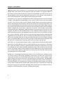
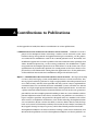
2 Related Work
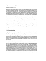
2.1 Introduction
Distributed processing was heralded as a key distinguishing feature of WSNs with respect to
traditional sensor acquisition systems. In terms of energy consumption, processing data on a
sensor node is cheaper than transmission of the data. In Section 2.2 we present the work that
is closest to our approach.
Wireless sensor networking is a large field, encompassing the physical deployment of the
hardware, the design of the application layer software, the optimized middleware and networking protocols down to the MAC layer, energy efficient hardware and even research and
development of new radio technologies. In the rest of this chapter we clarify how WSNs
relate to other wireless communication technologies and introduce the various sub-fields
necessary to make a complete WSN application. This information is in particular necessary to
understand the key elements to reduce energy consumption in WSNs and shows that really
efficient solutions can hardly be implemented by a single specialist.
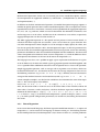
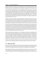
2.2 State of the Art
Guestrin et al. [46] have proposed a model based on linear regression that exploits spatiotemporal data correlation. Their approach uses this model in conjunction with Gaussian
elimination to reduce the amount of data sent over the sensor network. Basically, they model
the sensor data as a polynomial function of the sensor’s geographical position and the sampling
time. They use a least mean squares (LMS) algorithm to find the coefficients for a best fit to the
sensor data. Their implementation runs entirely within the WSN. An important contribution
of their work is a distributed algorithm to calculate the solution to the LMS problem in a
distributed fashion. The network transmits the model coefficients describing the observations
in the network to the sink. An application on the sink can then approximate values of the
observations anywhere within the network. Using this linear regression model enables a
significant reduction of the amount of data being transmitted in the network. Although their
7
Chapter 2. Related Work
approach proves to be very effective, it is intrinsically tied to the specific linear regression
model. Their work cannot easily be adapted to other data models. Our approach differs in
that we do not want to limit ourselves to a single sensor data model, but rather we want to use
existing models, such as the one proposed by Guestrin et al.. Users of our system should not
have to manually optimize a WSN application for their specific model.
Deshpande et al. [31] present a model based on time-varying multivariate Gaussian random
variables. Their approach, dubbed BBQ, treats sensors as multivariate Gaussian random
variables. If the statistics of the Gaussian random variables (mean and covariance matrix) are
known, then knowing the outcome for some of the variables in a particular experiment also
increases the knowledge about the likely outcome of the unobserved variables. BBQ estimates
the statistics of the sensors and then uses them to derive the likely outcome of sensor readings
without sampling the actual sensors. When the user queries a sensor with a given qualityof-information (QoI) requirement, BBQ determines a query plan for a set of sensors to be
sampled, such that the desired information can be estimated with the required accuracy
while minimizing the energy consumption for querying the sensors. All calculations are done
on a gateway computer, and the sensors are queried using traditional WSN communication
approaches such as TinyDB [76]. BBQ is not designed to be distributed among the nodes in a
WSN or to use models other than the one based on multivariate Gaussian random variables.
Again, our approach differs in that we want to give the user the choice of the model to be used.
We also focus on model processing being done at least partially inside the WSN.
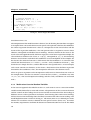
MauveDB [32] is an extension of Apache Derby, an open source relational database implemented in Java. MauveDB offers the user a novel kind of view that calculates its data based
on a sensor data model. Currently, supported models are based on either linear regression
or correlated Gaussian random variables. Model processing is done entirely on the back-end
system. MauveDB is similar to our approach in that it allows processing to be based on a
variety of data models. However, MauveDB runs exclusively on the back-end, while we focus
on model processing inside the WSN.
TinyDB [76] is a framework based on TinyOS that lets users see the WSN as a database. Querying sensors results in data being acquired by the network. In some cases, queries using
aggregation functions are calculated partially inside the network. TinyDB supports aggregation, energy-aware query constraints, and continuously running queries. TinyDB differs
from our approach in that it was never aimed at model-processing. To take advantage of
sensor data models a user would need to carefully craft the query to the network, necessitating
a deep understanding of how TinyDB works and how the query would best be composed.
The query language is based on SQL and might not be intuitive for users of WSNs without a
computer-science background. TinyDB is no longer maintained.
8
2.3. Wireless Networking Approaches
2.3 Wireless Networking Approaches
There are many commonly known wireless networking approaches. As they often lead to confusion when talking about wireless sensor networks, the most common wireless networking
techniques are briefly introduced and the main differences to WSNs are presented.
2.3.1 WiFi
WiFi, commonly known as wireless local area network (WLAN) or simply wireless network, is a
wireless network based on the IEEE 802.11 standards and is the wireless extension of wired
computer networks. Although not limited to this mode of operation, WiFi networks are mostly
used in managed mode, meaning that there is one or several base stations providing access to
a traditional wired network, and clients of the network establish a one-hop connection to a
base station. WiFi networking hardware can be used for multi-hop mesh networks (see WMN
and MANET) and even for some types of WSNs [71, 82].
2.3.2 Bluetooth
Bluetooth [109, 17] is a wireless communication technology for transmitting data over short
distances. It was initially designed to replace serial data cables. Bluetooth communication
is implemented as a master-slave protocol where a master device can communicate with up
to 7 slave devices. Communication between two slave devices passes through the common
master device. Multi-hop communication (so-called scatternets [11, 90]) can be achieved by a
device being part of multiple piconets, either as a master in one network and a slave in another
network, or as slave in multiple networks. Because Bluetooth was not really designed as a
multi-hop networking architecture, it is not commonly used for WSNs, although at least one
WSN hardware platform using Bluetooth exists [18, 15].
2.3.3 Wireless Mesh Network
A wireless mesh network (WMN) [49] typically consists of nodes using WiFi in ad-hoc mode
to communicate with each other over multiple hops. WMNs are used to network computers
in places where a wired network is not possible or too costly and where not every node can
communicate with every other node or with a central base station. WMNs can be used, for
instance, to provide Internet access to a whole town. Research in the area of WMNs focuses on
optimal routing.
2.3.4 Mobile Ad-hoc Networks
Mobile ad-hoc networks (MANETs) [62, 92, 77, 22] are essentially WMNs where the nodes
are mobile. The idea is to provide network access in areas with spotty network coverage, for
9
Chapter 2. Related Work
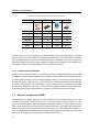
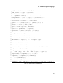
Table 2.1: Different classes of wireless networks.
RFID
Mote-class
PDA-class
MANET
RAM
-
∼10 KB
∼10 MB
∼1 GB
Storage
∼1 KB
∼1 MB
∼1 GB
∼100 GB
Speed
-
∼10 MHz
∼500 MHz
∼3 GHz
Lifetime
-
∼1 year
∼1 week
∼5 h
Bandwidth
∼100 bps
∼100 Kbps
∼10 Mbps
∼50 Mbps
Range
∼10 cm
∼30 m
∼100 m
∼100 m
instance, to enhance the network access to mobile phone networks inside buildings. The more
devices there are, the more robust the network should become. Since the devices are mobile,
they are typically battery-powered. Research in the area of MANETs focuses on routing in an
inherently mobile network, on battery-lifetime, and on how participants in the network can
be properly compensated for providing service to other participants.
2.3.5 Wireless Sensor Networks
Wireless sensor networks (WSNs) [3] are made up of sensors equipped with a low-power radio
transmitter to communicate their readings. Because of the low-power radio, communication
is mostly from the sensors to a data collection point (sink). As most WSNs run on batteries
or other low-power energy sources, research on WSNs is mainly concerned about reducing
the energy consumption. One of the biggest energy consumers in a sensor node is the radio
module (see Chapter 6), and hence, research tries to optimize communication, including
transmitting only relevant information by preprocessing data already in the network.
2.4 Device Categories for WSNs
Depending on the application, there are many different device configurations that can be
used for a WSN. Some installations have access to external power sources and thus can use
high-power radio modules, other installations will only be used for a few days and thus saving
energy is not important as long as the data is transmitted as fast as possible. Some installations
will have to run for years and only transmit a few bytes every day. The hardware capabilities of
WSNs can be broadly classified into four categories: radio-frequency identification, mote-class,
PDA-class, and laptop. The categories are summarized in Table 2.1.
10
2.4. Device Categories for WSNs
2.4.1 Radio-frequency Identification
Radio-frequency identification (RFID) systems consist of RFID tags and RFID readers. An
RFID reader beams energy to the tags it wants to read. In the original form, a tag becomes only
active when it receives this external energy. It then waits for the reader to transmit a request.
If the request matches the tag’s ID, it answers the request. RFID was designed to replace bar
codes. The advantage of RFID over bar codes is that the tags, replacing bar code stickers,
can be read without a line of sight. In a manufacturing environment, the contents of a box
containing different items can be scanned in a single pass without needing to open the box.
RFIDs are probably best known for their uses as wireless or touchless ski passes, or as access
cards to secure buildings. Most modern cars use RFID to identify ignition keys as an additional
anti-theft system. There are active RFID tags, which use a battery to boost the transmission
range and might do some processing and sensing even when not being read. RFID systems
are not typically used for WSNs, but they are sometimes mentioned in this context. They are
the WSN devices with the fewest resources and capabilities. RFID does not support multi-hop
communication.
2.4.2 Mote-class WSNs
The term mote was coined in the SmartDust project [96] as an allusion to dust motes. The
goal of the project was to create a sensor network consisting of devices smaller than a cubicmillimeter (and thus being considered dust). The term is an allusion to dust motes and
designates small sensor nodes. The typical mote is much larger than a cubic-millimeter, and
usually about the size of a pair of AA batteries.
2.4.3 PDA-class WSNs
Some people argue that it takes a while for research to bear fruit, that in this time technology
will progress, and that by the time sensor networks will become a commercial success, the
small sensor devices will have capabilities similar to today’s personal digital assistants (PDAs)
or smart phones. In order to experiment with networks with such capabilities, PDAs are used.
2.4.4 Laptops
The other extreme class of sensor network devices is laptops with built-in WiFi networking
cards. WSNs based on laptops are typically only used as proof-of-concepts, and their networking approaches are usually based on WMNs or MANETs. Laptops and embedded systems
might be used in other WSN installations as gateways, potentially connecting remote locations
via satellite or cell phone links.
11
Chapter 2. Related Work
2.4.5 Conclusion
Most literature about WSNs concerns mote-class or PDA-class networks. Compared with
mote-class networks, the devices in PDA-class networks have much more memory and higher
processing power. While indeed microprocessors have become much more powerful in the
past, the progress in battery capacity or in radio range of wireless transmitter is much slower.
The battery is typically the dominating factor for the size of sensor devices. While progress
in the miniaturization of all components of a sensor node can indeed lead to more powerful
networks, for some applications it is also interesting to just have smaller devices with the same
capabilities. Mote-class networks have to deal with much bigger restrictions, and approaches
developed for these limited devices can help to improve algorithms for more capable networks.
While the results of this thesis are not specific to any particular class of devices, the work
presented here has been done with battery-operated multi-hop mote-class sensor network in
mind.
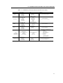
2.5 Hardware Devices for Mote-class Sensor Networks
While power consumption depends to a large part on the radio module, we have shown in [21]
that proper handling of microcontroller sleep modes can have a significant impact on overall
power consumption, especially for very low-power applications. We show in Chapter 6 that
hardware choices have a significant impact on power consumption. To minimize power consumption, adapting a program based on the characteristics of the hardware is necessary. We
present here the most common hardware platforms for generic WSN research. Other platforms
in use typically have very similar characteristics, as they, e.g., use the same microcontroller or
the same radio interface.
Virtually all current WSN hardware platforms are inspired by the original Mica [52] platform.
There are a number of direct descendants of the original Mica mote (in chronological order):
Mica2 / Mica2Dot, MicaZA, and Iris. These platforms, which are compatible with respect to
the hardware interfaces (e.g., for connecting external sensor boards), form the Mica-family of
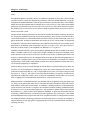
motes. A list with the main characteristics of the devices we studied in this thesis is shown in
Table 2.2.
The Mica2 platform [12] is the successor of the original Mica platform developed at the
University of California, Berkeley, which essentially defined the concept of a sensor node.
The Mica2 platform is probably the oldest platform that was commercially available and
has been used extensively in universities worldwide. The Mica2 platform uses the Atmel
ATmega128L microcontroller, which is well-known amongst hobbyists. In addition, it uses
the Texas Instruments (TI) Chipcon CC1000 radio, which is a low-power byte radio, thus
sending and receiving individual bytes at a time. This gives the platform a unique control over
low-level protocols, such as the media access control (MAC) protocol. The Mica2 platform
also introduced an interface configuration for sensor boards that is compatible amongst a
number of different sensor node types (Mica2 [12], MicaZ [14], Iris [60]) and adapters [97] exist
12
2.5. Hardware Devices for Mote-class Sensor Networks
Table 2.2: Commonly used sensor devices for mote-class WSNs
Mica2
MicaDot
BTnode rev. 3
MicaZ
Iris
TelosB
(Tmote Sky [87])
(Tmote Invent)
Microcontroller
Atmel ATmega128L
8 MHz
4 KiB RAM
128 KiB Flash
4 KiB EEPROM
Atmel ATmega128L
7.3 MHz
64 KiB RAM
128 KiB Flash
4 KiB EEPROM
Atmel ATmega128L
8 MHz
4 KiB RAM
128 KiB Flash
4 KiB EEPROM
Atmel ATmega1281
8 MHz
8 KiB RAM
128 KiB Flash
4 KiB EEPROM
TI MSP430f1611
8 MHz (4.15 MHz for TelosB)
10 KiB RAM
48 KiB Flash
256 bytes EEPROM
Radio
TI Chipcon CC1000
868 MHz
76.8 Kbps
10 dBm (10 mW)
Comments
Connector for external sensorboards
TI Chipcon CC1000
868 MHz
76.8 Kbps
10 dBm (10 mW)
Zeevo ZV4002
(Bluetooth)
2.4 GHz
1 Mbps
4 dBm (2.5 mW, class 2)
180 KiB external RAM
Connector for external sensorboards
TI Chipcon CC2420 [113]
2.4 GHz
250 Kbps
0 dBm (1 mW)
Connector for external sensorboards
512 KiB external Flash
Atmel AT86RF230
2.4 GHz
250 Kbps
3 dBm (2 mW)
Connector for external sensorboards
512 KiB external Flash
Optional Sensors (TelosB/Tmote Sky):
• Temperature
• Humidity
• Solar irradiation
TI Chipcon CC2420 [113]
2.4 GHz
250 Kbps
0 dBm (1 mW)
Tmote Invent Sensors
• 2D accelerometer
• Light sensor
• Microphone
1 MiB external Flash
built-in USB interface
TinyNode 584 [35]
TI MSP430f1611
8 MHz
10 KiB RAM
48 KiB Flash
256 bytes EEPROM
Xemics XE1205
868 MHz
152.3 Kbps
12 dBm (16 mW)
Connector for external sensorboards
512 KiB external Flash
13
Chapter 2. Related Work
for other platforms (TelosB [58], MicaDot [13]).
The MicaDot platform [13] is essentially a Mica2 platform in a different form factor. It is
substantially smaller than the Mica2 and runs on a coin cell battery. The MicaDot cannot use
the same hardware interface configuration for sensor boards as the Mica2 platform, and thus
has its own interface design. Adapters exist to connect sensor boards for the Mica2 platform
to the MicaDot platform, although not every functionality can be replicated.
The power consumption of the Mica2 platform has been studied extensively and numerous
simulators exist to determine the power consumption of a particular protocol running on
this platform (e.g., [4]). However, one should be careful to not simply reuse these results for
newer platforms, as different hardware choices, especially with respect to the radio module
in use, can significantly alter the power-consumption behavior of a platform. As there are so
many publications based on the Mica2 platform, the platform remains relevant in research for
comparisons with previous work.
The BTnode platform [18, 15] was developed independently and approximately at the same
time as the Mica platform at the Swiss Federal Institute of Technology in Zurich (Eidgenössische technische Hochschule Zürich, ETH-Z). The hardware design of this platform is publicly
available. The design of the BTnode centers around the use of Bluetooth as a commercially
established communications standard. Bluetooth is not designed for multi-hop communication. Devices are grouped in piconets with a master and up to seven slaves. Mesh networking
is only possible if the devices support scatternets [11, 90], where a device is a slave in multiple
networks and optionally a master in one network. The communication approach in Bluetooth
is substantially different from the approach of a byte radio. Bluetooth uses frequency-hopping
(it constantly changes the frequency in a well-defined pattern) and all the essential lower-layer
link-level protocols are implemented in the radio module. The current revision of the BTnode
uses the TI Chipcon CC1000 as a secondary radio, and thus is able to communicate with the
Mica2 and similar motes.
The MicaZ platform [14] is the successor of the Mica2 platform. It uses the then new TI
Chipcon CC2420 radio [113], which implements the IEEE 802.15.4 physical layer [57], and thus
can use the ZigBee [130, 9] radio stack. It also means that the MicaZ platform can communicate
with the TelosB and Iris platforms. The CC2420 is a packet radio, meaning that it sends and
receives multiple bytes as a packet. The MicaZ includes an additional Flash memory to store
sensor readings. It uses the same hardware interface configuration as the Mica2 and thus can
use the same sensor boards.
The Iris platform [60] is the successor of the MicaZ platform. It uses the Atmel ATmega1281
microcontroller, which has more RAM and Flash, and the Atmel RF230 radio module. The
RF230 is also a packet radio implementing the IEEE 802.15.4 physical layer, and the Iris
platform thus can communicate with the MicaZ and the TelosB platforms. The RF230 has a
slightly higher transmission power than the CC2420 (3 dBm vs. 0 dBm). The Iris platform uses
the same hardware interface configuration as the Mica2 and thus can use the same sensor
14
2.6. MAC Layer
boards.
The TelosB platform [58] is the successor of the earlier Telos platform. The hardware design
of this platform is publicly available. The TelosB uses the TI MSP430 microcontroller. In
contrast to the Atmel ATmega series of microcontrollers used in many other platforms, this
is a 16-bit microcontroller, it uses less power when active, and it has shorter wake-up times
from low-power modes. As we concluded in [21], a microcontroller has to periodically wake
up, and thus the power consumption when active is important even if the microcontroller has
an otherwise low duty-cycle. The TelosB platform uses the TI Chipcon CC2420 radio module
and is therefore compatible with the IEEE 802.15.4 physical layer. The TelosB platform has
an integrated USB interface and does not need additional programming or communication
hardware to connect to a desktop computer. The TelosB optionally comes with a set of onboard sensors for visible and infrared light, humidity, and temperature. Because of its open
design, the TelosB platform has been adopted by different manufacturers. A commonly found
variant is the Tmote Sky, which is the TelosB platform manufactured by the former Moteiv
company. Moteiv also produced a nicely packaged version called Tmote Invent, which came
in a futuristic-looking plastic casing (similar to a USB memory module), used a rechargeable
battery (recharged by plugging the device into a USB port) and included a number of different
sensors, such as an accelerometer, a microphone and a light sensor.
The TinyNode [35] from Shockfish SA, a spin-off from the Swiss Federal Institute of Technology
in Lausanne (école polytechnique fédérale de Lausanne, EPFL), uses the TI MSP430 microcontroller and the Xemics XE1205 radio module. The TinyNode platform has one of the highest
transmission powers amongst the embedded sensor networking platforms and, depending
on the environment, boasts a transmission range of more than 1 km. The TinyNode platform
is oriented towards environmental monitoring in isolated areas, and interface boards are
available that allow the platform to communicate with a home network over GPRS.
2.6 MAC Layer
The media access control (MAC) layer manages access to the medium (the “air waves”). When
two or more senders transmit simultaneously, their transmissions interfere with each other
and receivers often cannot decode any of the transmissions. This situation is called a collision.
The MAC layer is responsible for minimizing the risk of collisions. For WSNs, the MAC layer
also plays an important role in managing the power consumption of the radio. Low-power
radios, like the ones often used in WSNs, consume a significant amount of energy not only
when transmitting data, but also when receiving data, or simply when listening on the channel
for new transmissions. An ideal data transmission with minimal energy consumption would
be the transmitter and receiver turning on at the same time, the data being transmitted without
error, and then the two radio interfaces turning off again. In reality, this ideal is never fully
achieved as sensor nodes need to synchronize, and it is usually not known in advance when
new data is ready.
15
Chapter 2. Related Work
If we define wasted energy as energy consumed by the radio interface for purposes other
than transmitting the actual data, then there are four main causes for wasting energy [125]:
(1) collisions - two devices transmitting at the same time and interfering which each other’s
transmission, (2) overhearing - a device receives data that is not addressed to that device, (3)
control packets - data transmissions that do not carry application data but are rather used
for network management (and might not be needed with a different protocol), and (4) idle
listening - having the receiver activated and waiting for incoming packets when there are no
transmissions ongoing.
Because of the impact the MAC layer has on power consumption, research has focused on MAC
layer protocols, and this resulted in a large number of such protocols. The two main categories
of MAC layer protocols are synchronous and asynchronous protocols. In the following, a small
selection of the most important MAC layer protocols is presented.
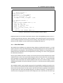
One of the first MAC layer protocols for WSNs is the Sensor-MAC (S-MAC) [125]. The S-MAC
regularly puts the radio interface in a sleep mode and loosely synchronizes wake-up times
between neighboring nodes. In addition, it uses a ready-to-send/clear-to-send (RTS/CTS)
message exchange to minimize the risk of collisions. A node that is too far away from the
sender to overhear the transmissions but is close enough to interfere with them is called a
hidden terminal. The problem of the hidden terminal can be overcome with the RTS/CTS
exchange, where the sender first signals its readiness with an RTS frame, and the receiver
then signals in return its readiness with a CTS frame. Other nodes in the vicinity of either the
sender or the receiver (including a potential hidden terminal) will be aware of the subsequent
transmission when they overhear either an RTS or a CTS frame. In addition, when a node
receives an RTS or CTS frame and is not involved in the subsequent transmission, it can turn
off its radio for the duration of the transmission.
The Berkeley MAC (B-MAC) [98] protocol is fully asynchronous and was for a long time the
standard MAC layer protocol for TinyOS. Nodes sleep and wake up periodically to sample
the channel and check for ongoing transmissions. If the channel is idle, the nodes go back to
sleep. To ensure that the destination node will wake up and receive a message, a transmitting
node has to send a preamble that is longer than the sleep period of the destination node. Any
node overhearing the preamble will stay awake until it receives the actual data transmission.
This mechanism is called low-power listening (LPL). When a node wants to send data, it first
waits for a random period (to statistically minimize the risk of collisions) and then samples the
radio channel. If the channel is idle, it starts the transmission, otherwise it waits for another
random back-off period.
The B-MAC works well on bit-radios, such as the TI Chipcon CC1000 used, e.g., on the Mica2
platform. However, packetized radios, radios that implement some MAC layer functionality
and transmit whole packets rather than a stream of bits, typically cannot send a continuous
long preamble. The X-MAC [19] protocol is specifically designed for packetized radios, such
as the TI Chipcon CC2420 or the Atmel RF230. Instead of a single long preamble, it sends a
16
2.6. MAC Layer
strobed preamble, which is a short preamble packet retransmitted as fast as possible for the
duration of the preamble period. The preamble packet contains the address of the destination
node. Nodes overhearing a strobed preamble not destined for them can thus go back to sleep.
The destination node can send an acknowledgement (ACK) packet after receiving a preamble
packet, thus shortening the preamble time. After the transmitting node sends its first message, if it has additional messages, it will use the normal random-back-off-approach to send
additional messages. Additional senders overhearing a strobed preamble for their destination
node can wait until the end of the preamble, and then transmit their own message using the
random-back-off approach. If the receiving node does not receive any new transmissions for
a period greater than the maximum back-off period, it can go back to sleep.
There are two BoX-MAC [86] protocols improving on the B-MAC and the X-MAC. Both protocols add cross-layer (physical and link layer) support. With the first BoX-MAC protocol, whose
operation is mostly based on B-MAC, a sending node transmits continuously small packets
with the destination address. This protocol uses the clear-channel assessment (CCA) from the
physical layer to sense whether a transmission is on-going. The use of the CCA enables very
short wake-up times when there are no transmissions. If a transmission is detected, the node
will stay awake to receive the preamble packet (link layer). If the node is the destination of
the data transmission, it will stay awake until it received the actual data packet. To enable the
short wake-up times, the sending node cannot wait for potential ACK packets, and thus the
preamble cannot be aborted.
The second BoX-MAC protocol is based on X-MAC, but sends the whole data packets instead
of short preamble packets. When a node receives the data packet, it can immediately abort the
retransmissions by sending an ACK. This reduces the control overhead: instead of receiving a
preamble packet, sending an ACK, and then receiving the data packet, the destination node
receives the data packet immediately. As opposed to the first protocol, with the second BoXMAC protocol a node wanting to transmit needs to observe the channel for a longer time,
as there are gaps between retransmissions to enable the destination node to acknowledge
the reception of the packet. Only if the channel remains inactive for a period longer than
the pause between two transmissions, the node can go back to sleep. This second BoX-MAC
protocol is currently the default MAC protocol for low-power operation in TinyOS.
A different approach is taken by the WiseMAC [37] protocol. The authors assume an infrastructure-based network, where the sensor nodes directly communicate with one of multiple access
points (AP). The APs are much more powerful and not energy constrained. A possible scenario
is home automation where there is a basic infrastructure provided by AP wired to a central
network, and low-power sensors and actuators (e.g., light switches) need to be connected to
this back-end. The authors further propose to use different MAC layer protocols based on the
direction of the communication (up-link to the AP or down-link to the sensor or actuator).
WiseMAC is a down-link protocol where the low-power devices use their own sleep schedules,
and the APs learn the schedules of the low-power devices to reduce unnecessary transmissions.
17
Chapter 2. Related Work
2.7 Routing
The routing requirements in a WSN differ significantly from other types of networks. By their
very nature, pure WSNs send most of the data from the individual sensors to a data collection
point, usually called sink. Little data is sent back to the nodes, e.g., configuration data and
end-to-end acknowledgments. Normally, there is no data exchange between arbitrary nodes
of the network. Optionally, data might be processed and modified on its way to the sink.
In wireless networks, one wishes to minimize transmissions to save bandwidth and energy.
Often, routing paths are chosen, such that the total number of transmissions for a single message is minimized. Many routing protocols use a measure called expected transmission count
(ETX, see for example [95]) that indicates how many times a packet needs to be transmitted on
average until it is correctly received by the receiver. If p s is the probability that a transmission
is successful, then the expected number of transmissions (ETX) is expressed as the sum of
all possible transmission numbers (until success) times the probability that the transmission
is successful. If we assume that a message can be retransmitted an infinite number of times
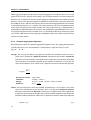
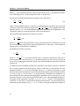
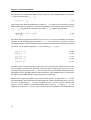
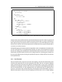
until it succeeds, ETX can be calculated as:
ETX =
∞
X
i =1
i (1 − p s )(i −1) p s =
1
.
ps
(2.1)
Optimal routing protocols using ETX might choose routes with a higher hop-count if the
individual links are of good quality. Suppose that two nodes n 1 and n 2 want to exchange messages. They can directly communicate, but they only have a success rate of 0.25 %, meaning
that on average a message needs to be transmitted four times to be correctly received by the
other node (ETXn1 ,n2 = 4). There might be an intermediate node n 3 which has better link
qualities to the two nodes, for example ETXn1 ,n3 = 1.2 and ETXn3 ,n2 = 1.3. Even though the
path n 1 → n 3 → n 2 involves one more hop than the path n 1 → n 2 , on average a message is
only transmitted 2.5 times, and thus this longer path would be preferred. The collection tree
protocol (CTP) [43] in TinyOS is a protocol that establishes routing paths with minimal ETX
from any node to a sink node.
2.8 Transport Layer / Middleware
A lot has been written about middleware for WSNs. An overview of middleware issues can be
found in [126, 124, 47, 102, 84].
To facilitate the interaction with WSNs, an interesting approach is to see the WSN as a
database [16]. Sensor readings are queried as if they were stored on a fixed medium. Instead of reading the data from a hard drive, the actual sensor nodes are queried. Two such
device databases based on SQL are the tiny aggregation service (TAG) [75] and TinyDB [76].
A slightly different approach is demonstrated with Asene [131], an implementation of an active
18
2.8. Transport Layer / Middleware
database inside a WSN. It uses publish/subscribe (see Section 2.8.1) to communicate among
nodes. The basic principle of Asene is to wait for events, then evaluate a condition and, if the
condition is true, execute a given action.
The shared memory paradigm, in particular in the form of tuple spaces, is another form of
middleware that has been tried for WSNs [29, 33]. A more complex approach to middleware is
mobile agents [65, 89, 66]. The idea here is that instead of sending a query to the network, a
small piece of code is sent, which gets then executed on the nodes, queries the the desired sensors, preprocesses the obtained data and then sends it back to the sink. Most implementations
we found in the literature are based on Java and run on PDA-class networks. For mobile agents
to properly work on mote-class networks, the sensor nodes must either support partial code
updates, e.g., as provided by TinyCubus [80, 81], or must implement some sort of interpreter
or virtual machine that can execute code on the fly, such as [41, 69, 21].
Titan [74], the tiny task network, assigns processing tasks to individual nodes such that the
data traveling from the source sensor nodes to the sink is being processed step by step. The
distinguishing feature of titan is the ability to distribute computing-intensive tasks among
several nodes that otherwise could not be executed on a single node as it would not have the
necessary resources.
2.8.1 Publish/Subscribe
Wireless sensor networks are dynamic by nature. New sensors will get added and existing
sensors might fail or run out of battery. As such, communication within a sensor network
needs to cope with changes. A solution to deal with the complexity of such changes is datacentric communication approach [38], in which information is delivered to the consumers
not based on their network addresses, but rather as a function of their contents and interests.
Publish/Subscribe messaging systems [40] are well-known examples of data-centric communication and are widely used in enterprise networks, mainly because of their scalability and
support of a dynamic application topology. These features are achieved by decoupling the
various communicating components from each other, such that it is easy to add new data
sources/consumers or to replace existing modules [91].
MQTT-S [56] is an extension of the open publish/subscribe protocol message queuing telemetry
transport (MQTT) [88]. It is designed for operation on low-cost and low-power sensor devices
and running over bandwidth constrained WSNs. MQTT-S provides a simple but scalable
communication means for interacting with a large number of sensor devices and enables a
seamless integration of the WSNs into traditional networks.
TinySIP [68] is an extension of the well-known session initiator protocol (SIP) for WSNs.
TinySIP supports session semantics, publish/subscribe, and instant messaging. TinySIP offers
support for multiple gateways. Most communication is done by addressing individual devices.
As device addresses are related to the gateway being used, changing the gateway on the fly is
19
Chapter 2. Related Work
difficult.
Mires [110] is a publish/subscribe architecture for WSNs. Basically, sensors only publish
readings if the user has subscribed to the specific sensor reading. Messages can be aggregated
in cluster heads. Subscriptions are issued from the sink node (typically directly connected to a
PC), which then receives all publications.
DV/DRP [48] is another publish/subscribe architecture for WSNs. DV/DRP stands for distance
vector / dynamic receiver partitioning. Subscriptions are made based on the content of the
desired messages. Subscriptions are flooded in the network. Intermediate nodes aggregate
subscriptions. They forward publications only if there is an interest for this publication.
Because of the complexity of matching subscriptions to arbitrary data packets, it would be
difficult to implement this protocol on the devices targetted in this thesis.
Messo and Preso [103] are two complementary publish/subscribe protocols for WSNs. Messo
allows data to be collected from sensors in a WSN, whereas Preso allows data to be sent to
actuators in the WSN. Messo and Preso rely on an external broker. Messo and Preso differ
from MQTT-S in that they do not establish individual connections between the devices and
the broker. Their implementation takes advantage of the possibility of processing data inside
the WSN. Each node decides locally whether to forward a message. If data is collected with
Messo, nodes that relay messages can also combine multiple messages. Currently, Messo and
Preso rely on predefined topics. They cannot dynamically add new topics. They also require a
single gateway.
2.9 Aggregation / Compression
A sensor network can provide a large number of individual sensor readings. Often, it is
not interesting to see every single reading, but rather one would like to have a summary of
the information. Aggregation [1, Section 2.2.3] is often used to calculate such summaries.
For a simple network monitoring the temperature in a building, one might want to see the
minimum, maximum and average temperatures. Minimum, maximum and average are
examples of aggregation operators that take a list of values as input and produce a single
result. A simple approach to obtain the desired values from the building monitoring network
would be to collect all the readings in a central computer (the back-end), and then apply
the aggregation operator to the list of sensor readings. A more efficient approach to, e.g.,
determine the minimum temperature would be to have each node only forward the smallest
temperature value it encountered. For many aggregation operators it is possible to find an
efficient distributed implementation.
Distributed aggregation as described by Madden et al. [75] works as follows. Each node
participating in the computation holds a partial state record, which it initializes with its own
sensor readings using an initializer function i . A node will receive the partial state records
from its children and merge them with its own partial state record using a merging function
20
2.9. Aggregation / Compression
f . On the back-end, the actual result of the aggregation operator is obtained by applying the
evaluator e to the final partial state record. While this concept of aggregation is very generic,
the partial state record is typically a set of n real numbers ( n ), while the set of numbers (e.g.,
sensor readings in a WSN) and the final value of the aggregation operator normally are real
numbers ( ). Thus, since i is used to initialize the partial state record, i : → n . The merging
function m merges multiple partial state records, m : { n , n } → n . Finally, the evaluator
e calculates the final value of the aggregation from the partial state record representing the
merged data from the whole set and produces a single value, e : n → .
❘
❘
❘ ❘
❘
❘
❘ ❘
❘
2.9.1 Problems of Distributed Aggregation
Distributed aggregation works well in principle. In real implementations, problems occur due
to packet loss, due to packet retransmission and hence packet duplications, and due to the
size of partial state records becoming too large. Not every aggregation operator is affected
by the same types of problems, and not every type of problem is equally important for the
different operators.
For many aggregation operators, the loss of a single sensor reading does not affect the result
much, the operator will still give a good approximation of the desired value. Some aggregations
are more sensible to the loss of sensor readings than others, and in a wireless sensor network
(WSN) the loss of a packet close to the sink usually means the loss of the data of a whole
subtree. To avoid this problem a simple solution is to implement retransmissions. WSNs differ
from traditional networks in that their links can change over time due to changes in the radio
environment (e.g., changing weather conditions or moving obstacles, such as persons and
cars) or due to node failures. To increase the reliability of the network, data is often transmitted
over multiple paths, which then might lead to receiving the same information multiple times.
Some aggregation operators, like min and max, are naturally insensitive to data duplications,
while most standard implementations of other aggregation operators are affected by it. It is
possible to transform some of the standard implementations to duplicate-insensitive implementations, usually by transforming them to a probabilistic approach at the cost of accuracy.
Considine et al. [27] showed, based on earlier work on estimating unique entries in a database
done by Flajoulet et al. [42], the basic idea for probabilistic implementations. They also show
how to extend their approach to probabilistic counting and summing, which can be used as
basic operators for many other aggregation operators, like average or histogram.
Manihj et al. [78] describe an interesting approach where a duplicate-sensitive, exact implementation of some aggregation operators is used at the periphery of the WSN. Towards the
sink, the expected impact of data loss increases as the loss of a single packet would mean the
loss of the data from a whole subtree. Once the expected loss based on the transmission error
rate and the amount of data in a packet passes a threshold, the aggregation implementation is
switched to a duplicate-insensitive, probabilistic implementation.
21
Chapter 2. Related Work
Some aggregation operators do not have a partial aggregate of a fixed size. The count unique
operator, for instance, requires one to keep a list of unique elements to avoid counting an
element twice, and hence the size of its partial aggregate is dependent on the number of unique
elements. The median operator requires an ordered list of all elements to pick the element in
the middle of the list, and thus the size of its partial state record is proportional to the number
of contributing elements (i.e., sensors). For some operators, there exist implementations
with a fixed-size partial state record, usually with a loss in precision (e.g., implemented as
a probabilistic approximation). For instance, the probabilistic approximation of the count
unique operator presented by Considine et al. [27] (mentioned above) has a fixed-size partial
state record, while for the median operator no implementation with a fixed-size partial state
record is currently known.
2.9.2 Common Aggregation Operators
We briefly present the most common aggregation operators here. The aggregation operators
typically operate on a set of real numbers X and produce a single real value as result:
agg : { , . . . , } → .
❘
❘ ❘
Average: The average (or shortly avg) operator calculates the arithmetic mean of a set of
values. The avg operator is duplicate-sensitive. The partial state record is of fixed size
and consists of two numbers. The required size to represent the full range of possible
values for these two numbers depends on the number of elements (count) and the
values of the elements (sum). There exists a duplicate-insensitive form of this operator.
avg(X ) =
X
xi
x i ∈X
(2.2)
|X |
Partial state record:
Initializer:
Merger:
Evaluator:
{sum, count}
i (value) = {value, 1}
m(a, b) = {a.sum + b.sum, a.count + b.count}
a.sum
e(a) = a.count
Count: The count operator counts the number of elements in a set of values. The actual
values have no influence on the outcome. The count operator is duplicate-sensitive.
The partial state record is of fixed size and consists of a single number. The required size
to represent the full range of possible values for this number depends on the (maximum
possible) number of elements. There exists a duplicate-insensitive form of this operator.
count() = |X |
22
(2.3)
2.9. Aggregation / Compression
Partial state record:
Initializer:
Merger:
Evaluator:
{count}
i (value) = {1}
m(a, b) = {a.count + b.count}
e(a) = a.count
Min: The min operator determines the smallest value in a set of values. The min operator is
duplicate-insensitive. The partial state record is of fixed size and consists of a single
number. The required size to represent the full range of possible values for this number
depends on the full range of permissible values of the elements.
min() = x i ∈ X s.t.∄(x j ∈ X , x j < x i )
Partial state record:
Initializer:
Merger:
Evaluator:
(2.4)
{min}
i (value) = {v al ue}
m(a, b) = {(a.min ≤ b.min) ? a.min : b.min}
e(a) = a.min
Max: The max operator determines the largest value in a set of values. The max operator is
duplicate-insensitive. The partial state record is of fixed size and consists of a single
number. The required size to represent the full range of possible values for this number
depends on the full range of permissible values of the elements.
max() = x i ∈ X s.t.∄(x j ∈ X , x j > x i )
Partial state record:
Initializer:
Merger:
Evaluator:
(2.5)
{max}
i (value) = {v al ue}
m(a, b) = {(a.max ≥ b.max) ? a.max : b.max}
e(a) = a.max
Sum: The sum operator determines the sum of all values in a set of values. The sum operator is duplicate-sensitive. The partial state record is of fixed size and consists of a
single number. The required size to represent the full range of possible values for this
number depends on the full range of permissible values of the elements multiplied by
the maximum number of elements. There exists a duplicate-insensitive form of this
operator.
sum() =
X
xi
(2.6)
x i ∈X
23
Chapter 2. Related Work
{sum}
i (value) = {v al ue}
m(a, b) = {a.sum + b.sum}
e(a) = a.sum
Partial state record:
Initializer:
Merger:
Evaluator:
Median: The median operator determines the value in the middle of an ordered set of values.
If the set contains an even number of values, the median operator determines the
arithmetic average of the two values in the middle of the set. For some applications,
median can be used instead of avg, especially if the set of values contains extremely
large or small numbers. The partial state record is duplicate-sensitive, has a variable
size, and consists of all the elements so far encountered. There is no known duplicateinsensitive form or implementation with a fixed-size partial state record of this operator.
As the sensor readings in X might arrive in any order, we first need to make an ordered
set Y = {x 1 , . . . , x n } where n = |X |, ∀y i ∈ Y → y i ∈ X and y i ≤ y i +1 ∀i = 1, . . . , n − 1.
median() =
y ⌊ n2 ⌋ + y ⌈ n2 ⌉
2
(2.7)
Mode: The mode operator determines the most frequent element in a set. There might be
multiple elements with equal occurrences, so the mode operator might not find a single
value. The partial state record is duplicate-sensitive, has a variable size, and consists
of a list of all unique values encountered, and for each value a count indicating how
often this value was encountered. There is no known duplicate-insensitive form or
implementation with a fixed-size partial state record of this operator.
First we must introduce a function that counts the number of occurrences of a given
element a:
count(a) =
X
δa,xi
(2.8)
x i ∈X
Then we can say that the mode of a set X is:
mode() = x i ∈ X s.t.∄(x j ∈ X , count(x j ) > count(x i ))
(2.9)
Count Unique: The count unique operator counts how many unique values are in a set of
values. The partial state record is duplicate-sensitive, has a variable size, and consists
of a list of all unique values encountered. There exists a duplicate-insensitive form of
this operator.
We first need to define a function to determine whether an element is the first occurrence
in the set:
(
1 if ∄(x j = x i , j < i ),
(2.10)
first(i ) =
0 otherwise
24
2.10. Simulating Energy Consumption
We then count an element only if it is the first occurrence (n = |X |):
count_unique() =
n
X
first(i )
(2.11)
i =1
Histogram: The histogram operator splits the range of permissible values into a number of
buckets. It then sorts the elements of a given set of values into the buckets and counts
how many elements are in each bucket. The partial state record is duplicate-sensitive
and has a fixed size. The size of the partial state record depends on the number of
buckets. There exists a duplicate-insensitive form of this operator.
Min-k: The min-k operator determines the smallest k values in a set of values. The min-k
operator is duplicate-insensitive. The partial state record is of fixed size and consists
of k numbers. The required size to represent the full range of possible values for these
numbers depends on the full range of permissible values of the elements.
Max-k: The max-k operator determines the largest k values in a set of values. The max-k
operator is duplicate-insensitive. The partial state record is of fixed size and consists
of k numbers. The required size to represent the full range of possible values for these
numbers depends on the full range of permissible values of the elements.
2.10 Simulating Energy Consumption
An important part of developing a program for a distributed wireless sensor network is testing
the program. Testing on a real and distributed network is often difficult and time-consuming.
As an alternative, one can run the program in a simulator. Different simulators focus on
different aspects of the program execution: simulating the radio environment, simulating the
execution of the program, and simulating the exact behavior of the hardware when executing
the program.
Simulators for analyzing the behavior of a protocol in realistic conditions are NS2 [63] and
OmNet++ [119]. These simulators use complex radio propagation models, including path loss,
noise, interference, and fading. They are optimized to study the behavior and performance of
wireless protocols in different environments. The simulated radio devices do not need to be
stationary, the simulator can move them around in a programmable pattern. The protocol
under study must be implemented in a special language supported by the simulators. Most
such simulators (including NS2 and OmNet++) are designed to simulate WiFi radios and do
not support the specialized low-power radios used by most WSN platforms.
TinyOS [51], a commonly used operating system for mote-class WSNs, provides its own
simulation environment called TOSSIM [70]. A program written for TinyOS can be compiled to
run as a simulation. The program will then be compiled to run on the computer platform rather
than a specific WSN device platform. TOSSIM provides a means to run multiple instances of
the program and simulates the radio environment. Programs can display debugging messages.
25
Chapter 2. Related Work
As the simulation has to abstract some hardware features such as the radio module, the current
version of TinyOS only supports simulating MicaZ devices.
PowerTOSSIM [107] is an extension of TOSSIM to estimate the power consumption of a program. It works by logging every event that has an impact on power state changes, such as
turning on and off the radio and changing the power mode of the microcontroller. PowerTOSSIM modifies the code of the simulated program, such that it generates events at the
beginning and end of blocks of code. The execution time of these code blocks on the actual
microcontroller is calculated by finding the corresponding code in the binary for the target
platform and then adding up the known execution times of the individual instructions. The
final energy consumption is calculated by multiplying the power draw of the hardware in a
given state by the time the hardware is in this state, as determined from the logging of the
events. PowerTOSSIM is currently not available for TinyOS 2.x.
The most precise power consumption estimates can be obtained with a cycle-accurate simulation of the hardware. In a cycle-accurate simulation, the microcontroller’s behavior is
simulated for every cycle that it executes. These simulators thus run the actual binary code
compiled for the targeted platform. The first such hardware simulator for wireless sensor
networks was ATEMU [99]. ATEMU emulates the hardware of a Mica2 node and simulates
the radio environment. While ATEMU is capable of simulating whole networks with multiple
nodes, it does not scale well for networks larger than approximately 100 nodes. Avrora [115]
also simulates WSN networks at the hardware level. Avrora is implemented in Java and currently supports the Mica2 and the MicaZ hardware platforms. It takes advantage of the fact
that most WSN applications spend a significant part of the time in sleep-mode. Instead of
emulating every single clock tick to determine the next wake-up time, Avrora maintains an
event queue and can skip over inactive periods. This makes Avrora approximately 30 times
faster than ATEMU. Avrora has been shown to simulate networks of up to 25 nodes in real
time and was able to simulate networks of 10000 nodes. In Section 6.6 we describe how we
extended Avrora to also support the TelosB platform.
The decision for which simulator for WSNs to use depends largely on the goals of the simulation. For protocol evaluation, clearly one of the network simulators is most appropriate. If
one wants to debug the behavior of a program, a simulator on code execution is better suited
and might provide additional debugging options. In order to get a good estimated of the
power consumption of a program, a simulator operating at the lowest level possible and really
simulating the hardware characteristics is most appropriate. In spite of good simulations,
it is advisable to monitor the power consumption of the actual hardware [123], as there is
always a risk of hardware modifications or other unexpected details not being considered by
the simulation.
26
2.11. Conclusion
2.11 Conclusion
Although the processing capabilities of sensor nodes is considered a key distinguishing feature
of WSNs, to the best of our knowledge nobody has so far proposed a system that would allow
to separately define a-priory knowledge to then optimize in-network processing. In Section 2.2
we have presented projects that seem to share our ambitions.
WSN research is a very broad field with multiple subfields. In addition, there are various other
fields of research that are closely related to WSNs. To create power-efficient WSN applications,
one has to be an expert on different topics, such as MAC layer protocols, routing algorithms,
and distributed processing. In this chapter, we presented a selection of topics related to
WSNs, and in particular related to power consumption and distributed processing. The related
work presented here is essential for anyone wanting to study or implement energy-efficient
distributed processing for wireless sensor networks.
27
3 Sensor Data Models
3.1 Introduction
There are three main reasons why one would want to install a WSN:
1. To understand how the observed physical parameters behave,
2. to get feedback about the current status of the observed object, and
3. to detect when one’s assumption about the behavior of the parameters does not hold
anymore.
These three reasons correspond to the three ‘E’s from Chapter 1 on page 2: understanding a
physical system is exploration, continuously observing a system is exploitation, and detecting
anomalies is exception.
Sensor readings are normally not completely random, but correlated in time and space. Two
temperature sensors in the same room might have different readings, e.g., because they are
mounted at different heights off the ground. Readings from the same sensor will not jump
randomly over the entire temperature range but usually be close to the previous readings.
Similarly, the two sensors in the room will normally indicate temperatures that differ by no
more than a few degrees. If the temperature in the room is changed, the change will likely
affect the readings of both sensors. Thus, sensor readings are correlated in time and space.
The exact nature of the correlation depends on many factors, and WSNs can help to quantify
and potentially identify the nature of the correlation.
If one knows how the observed parameters behave, one might simply want to monitor the
parameters in order to adjust one’s actions based on the current situation. For instance, the
temperature measures in a room can be used to control the heating or cooling of that room.
Sometimes, the parameter one wants to monitor cannot directly be observed, but it can be
estimated based on the observation of other parameters. For instance, the evaporation rate of
29
Chapter 3. Sensor Data Models
a lake or glacier might not be measurable directly, but it can be calculated based on observed
humidity and solar radiation.
The behavior of a system might change over time. For instance, one could estimate the
temperature in a room based on the amount of sunshine that gets in through the window. But
one’s model of the room temperature might not hold anymore if the environment changes in
an unpredicted way, such as leaving the door or window open. Measuring multiple parameters
and verifying that the correlation between them holds over time can help to detect limitations
in one’s assumptions.
The principal role of a sensor network is to monitor the states of an underlying physical system.
Each individual sensor measures the magnitude of a physical characteristic of the system
at the point where it has been placed. Sensors are built such that their values are primarily
influenced by the physical parameter that they observe. The readings are also influenced by
other physical parameters as the characteristics of the sensor might change, e.g., with changes
in the ambient temperature. Brownian movements and thermal noise will introduce errors.
When transforming a sensor reading into a digital value, a quantization error is introduced.
Finally, a sensor is designed for a given value range. If the value of the physical parameter
under observation falls outside the range of the sensor, the sensor will report false readings.
Techniques to detect and handle anomalies in sensor readings exist, see for instance [128, 127].
In this thesis we assume that the measurement errors of sensors is small and negligible in the
context of our work. The sensor readings can thus be assumed to represent the actual values
of the physical parameter that the sensor monitors. To take the correlation of different sensor
readings into account, the behavior of the sensors or the physical system being monitored is
modeled.
A mathematical model aims at describing a system and its behavior by expressing the relationship of key elements within the system as a mathematical relationship. The same system can
have multiple models that describe different aspects. Additionally, there might be multiple
models describing the same aspects of a system, but with different methods. The description
of the system given by a model will in most cases not be absolutely accurate. Therefore, a
model describing a system is characterized by its complexity and its accuracy. If a system
needs to be modeled for a particular purpose, the set of acceptable models typically is the
subset of all models for that system where each model is accurate “enough” according to a
given criterion. Typically, the model chosen will be the model amongst all known models that
are accurate “enough” and which is the least complex.
Based on this definition we see that a model is based on a number of elements of interest
within a system. The model consists of a number of mathematical relationships between these
elements of interest. In addition, when choosing a model, we need an evaluation function
that measures the quality (or applicability) of the model to our problem set.
30
3.1. Introduction
The elements described by the model are represented as variables. There are six major types of
variables commonly used in models: input variables that are directly associated with a physical
property in the system, variables representing a state of the system or the model, parameters that configure a generic model for a particular system, random variables, independent
variables and output variables.
The aim of a sensor data model is to represent the sensor readings of a sensor network. As
such, the input variables are directly given by the sensors, where the values are the actual
sensor readings. The output variables are typically, but not necessarily, also related to the
sensors and represent predictions by the model. The state variables are model parameters
that are learned from the sensor readings. There might be configuration parameters set by the
user when setting up the model. The independent variables are used to query the model. The
random variables could be used instead of another variable whose value is not known. The
model would then be evaluated for different random values for this variable, and the outcome
could be averaged or analyzed for a specific value distribution.
In this document we assume that a sensor data model describes a physical system. The input
variables are the sensors placed at specific locations inside the system measuring a specific
physical property. Sensor values have a given range and resolution. It is often assumed that
the sensor readings are real values . Output variables can represent the model’s prediction
for a given sensor value, or they can be the sensor readings for a virtual sensor arbitrarily
placed within the system.
❘
The mathematical relationships in a sensor data model are basically two types of functions:
learning functions and prediction functions. The learning functions describe how to determine
the state variables for a given set of input values or sensor readings. The prediction function
takes a set of query parameters (independent variables) as input and then calculates (predicts)
the value of an output variable based on the query parameters and the state of the model
expressed in the model parameters. To compare different models supposedly describing the
same behavior, an evaluation function is needed that describes the accuracy or error of a
model.
One obvious method of classification relates directly to the data source of the model. The
model can express the data over time of a single sensor, the relationship between different
sensors at a given instance in time, or a combination of data from different sensors and
different instances in time. In addition, the sensors involved can all be of the same type, or
they could measure completely different characteristics of the system.
The other obvious method of classification relates directly to the output of the model. In [16]
the authors identify three different types of query for sensor data: long-term queries for
historical analysis, querying a specific information and getting alerts on the occurrence of
specific conditions. Long-term queries are for instance used if it is not yet clear what exactly is
expected of the data, and it should be analyzed with different methods at a later time. Certain
laws also require the storage of data to later prove that a given situation did not occur. Querying
31
Chapter 3. Sensor Data Models
a particular information can occur, for instance, if this particular information could clarify a
more generic situation potentially observed by other means, or if an alert was triggered.
There are three main benefits of processing parts of sensor data models within the sensor
network: selection of the interesting data and discarding the rest, in case of loss of data make
the system degrade the results gracefully, and compressing the data.
Modeling the sensor data can be done at two different levels. If it is possible to describe the
underlying physical system by a set of equations establishing a relation between geographical
coordinates and magnitudes of physical characteristics at these coordinates, then it is possible
to apply this deterministic model directly to the sensor data. If the description of the physical
system is too complex or unknown, then one may use well-known probabilistic models, such as
linear regression [46] described in Section 3.3 or Gaussian models [31] described in Section 3.4.
The aim of the work presented in this thesis is to take existing models and provide a framework
that allows to use such models for WSNs. As such, the models presented in this chapter are not
original work in the context of this thesis, and references are provided. We ignore the merits of
the individual models and focus on discussing how different categories of models can be used
to process sensor data in a distributed fashion inside a WSN.
3.2 Deterministic Models
Environmental scientists use modeling extensively. Deterministic models describe the state
of objects in a system (e.g., their temperatures). To predict the development of the system,
the state of the system is used to calculate the rate of energy (radiation) and mass (transport)
exchange. The exchange rate depends on the state of the system, e.g., there is more water
flowing out of a lake if the water level in the lake is high. Therefore, the state and the rate of
exchange form an ordinary or partial differential equation system.
The exact solutions even of simple models are often not known. Typical models are a complex
combination of different physical processes. For instance, the models used for weather
forecasts take into account solar radiation, wind, clouds, evaporation, and snow on the
ground. As solutions to such complex equation systems, if they exist, would themselves be
even more complex, the evolution of the system is calculated in small steps with numerical
approximations.
To predict the evolution of a physical system, the system’s parameters are modeled on an
equidistant grid. Sensor data from, e.g., a WSN is used to determine the initial values of the
system at the grid points. This initialization phase is called parametrization. The sensors are
typically not located on the exact grid coordinates, as e.g., geographic characteristics (mountains, rivers, cities) make it often impossible or at least difficult to place sensors there. Instead,
the values at the grid coordinates are typically interpolated from the available sensors.The
state of the system is then advanced by determining the exchange rate of radiation and mass
32
3.2. Deterministic Models
based on the current state, and then modifying the state based on this exchange rate over a
relatively short period of time, during which the exchange rate is assumed to be constant.
Research on deterministic models is ongoing (e.g., [7]), as progress in computer hardware
makes it possible to run simulation with more details and additional parameters. Some models,
e.g., the Navier-Stokes equation for fluid dynamics, are considered to be exact, but they cannot
be computed in a reasonable time for most of the interesting problems. Research thus tries to
find acceptable approximations that are faster to solve. Thus, even though one would think
that there is only one way in which physical systems interact, and that this interaction is
described by well-known physical equations, this deterministic interaction is too complex to
reasonably be computed. Current deterministic models are a simplification of the physical
reality, often using approximations instead of the full mathematical relationships, and ignoring
a part of the parameters of the system.
Today’s hardware for sensor nodes does not have the capacity to calculate the evolution of
deterministic models. A single node does not have enough memory to store the representation
of a whole system. Nodes could interact to cooperatively calculate the evolution of the system,
but this would involve heavy data exchange, which is too expensive in terms of latency and
energy consumption. For these reasons, the prediction of the evolution of physical systems is
done on the back-end system. However, part of the calculation for the parametrization of the
model can be done inside the WSN. This is often done with the help of probabilistic models
described in the next section.
We will model the wind flow over a mountain ridge as an example of a deterministic model1 .
We simplify the model as much as possible and concentrate on the key aspects of modeling.
Wind flowing over a mountain ridge, without changes in the flow rate or direction, would
normally form a steady-state system with little interest for modeling. The initial state of such
a system would also be difficult to determine. We therefore start without mountain (or with
a mountain with a height of 0 m), and the initial condition is easily known: the wind speed
is uniform in the whole system. Over time we let the mountain grow to a given height and
model how the wind changes and how turbulences are introduced. Further simplifications
include the simulation of only two dimensions (x and z), ignoring earth’s rotation, ignoring
thermal energy transfer (adiabatic flow), and letting the wind speed over the lower boundary
be constant (isentropic surface).
For an isentropic model the vertical coordinate is best expressed as the potential temperature
Θ, as this will greatly simplify many equations. The potential temperature in our case is given
by:
Θ=T(
pr e f
p
)R/c p ,
(3.1)
1 The material presented here is based on the course “Numerical Modeling of Weather and Climate” by Prof.
Christoph Schär and Prof. Ulrike Lohman, which the author followed in 2008 at ETH Zurich as part of the thesis
course work. We have personally performed the calculations and modeling of this example in the course project.
33
Chapter 3. Sensor Data Models
where p r e f is the referenece pressure, R the gas constant for dry air, c p the specific heat of dry
air at constant pressure, T is the temperature, and p is the pressure.
We thus get the horizontal momentum equation in the x-direction as:
¶
µ
Du
δM
=−
Dt
δx Θ
(3.2)
where u is the horizontal velocity, t is the time, x is the horizontal
³ ´x-coordinate, Θ is the vertical
D
δ
δ
coordinate expressed as potential temperature, D t = δt + u δx
is the simplified advection
Θ
operator, and M = φ + c p T is the Montgomery potential with φ being the Geopotential, c p the
specific heat of dry air at constant pressure, and T the temperature.
The two-dimensional equation of continuity is given as:
¶
µ
δσu
δσ
=0
+
δt
δx Θ
(3.3)
δp
where σ = − g1 δΘ is the isentropic density with g being Earth’s gravity, p the pressure, and Θ
the vertical coordinate expressed as potential temperature. t is the time, u is the horizontal
velocity, and x is the horizontal x-coordinate.
The hydrostatic relation is given by:
π=
δM
δΘ
(3.4)
´
³
p R/c p
where π = c p p r e f
is the Exner function with c p being the specific heat of dry air at
constant pressure, p the air pressure, p r e f the reference pressure, and R the gas constant of
dry air. M is the Montgomery potential, and Θ is the vertical coordinate expressed as potential
temperature.
It is difficult to find a symbolic solution to the equation system above. Instead, we simulate
this system by progressively advancing the time in small steps ∆t and calculate the next
horizontal velocity u t +∆t (x, Θ) and isentropic density σt +∆t (x, Θ) for each point in a grid
based on the current and previous values of the horizontal velocity and the isentropic density
(u t (x, Θ), σt (x, Θ), u t −∆t (x, Θ), and σt −∆t (x, Θ) respectively). To facilitate the calculations, we
also calculate for each grid point the Montgomery potential M (x, Θ), the pressure p(x, Θ),
the Exner function π(x, Θ), and the geometric height z(x, Θ). The topographic height (i.e.,
2
the height of the mountain) is given by z topo (x, t ) = ae (xi /b) , where x is the horizontal xcoordinate, t is the time, a is the maximum height of the mountain, b is the full width of the
mountain at half-maximum, and x i = i − n x /2 + 1 with n x being the number of grid-points in
34
3.3. Linear Regression
the simulation and i being an independent variable.
σt +∆t (x, Θ) = σt −∆t (x, Θ) −
1
3
∆t 1
( (u t (x + ∆x, Θ) + u t (x + ∆x, Θ))σt (x + ∆x, Θ)
∆x 2
2
2
(3.5)
1
3
1
− (u t (x − ∆x, Θ) + u t (x − ∆x, Θ))σt (x − ∆x, Θ))
2
2
2
µ
¶
1
∆t
1
3
1
1
u t (x + ∆x, Θ) u t (x + ∆x, Θ) − u t (x − ∆x, Θ)
u t +∆t (x + ∆x, Θ) = u t −∆t (x + ∆x, Θ) −
2
2
∆x
2
2
2
∆t
−
(M (x + ∆x, Θ) − M (x − ∆x, Θ))
∆x
(3.6)
3.3 Linear Regression
Linear regression2 is a method for finding a set of dependent variables such that the given
regression function best fits the data. As an example, let us assume that the temperature in a
WSN can be expressed as a simple function of the coordinates of the sensors and the time of
the readings. Our prediction function thus could be:
f (x, y, t ) = a 1 + a 2 x + a 3 y + a 4 t + a 5 t 2 ,
(3.7)
where
• f (x, y, t ) ∈
• (x, y) ∈
❘ is the prediction function,
❘2 are the coordinates representing the sensor position in a plane,
◆ is the discretized time, and
a 1 . . . a 5 ∈ ❘ are the model parameters.
• t∈
•
Linear regression is a method to find the values of a 1 . . . a 5 such that the overall error is
minimized. This is a very simple example, and much more complex functions can be used.
To formally define linear regression, let f () be the regression function, x 1 , . . . , x p the function
arguments, a 1 . . . a c the dependent variables, and g 1 () . . . g c () a set of functions that combine
the arguments of the outer function. The linear regression function then has the basic form:
f (x 1 , . . . , x p ) = a 1 g 1 (x 1 , . . . , x n ) + · · · + a c g c (x 1 , . . . , x n ) .
(3.8)
2 Linear regression is a standard mathematical tool and can be found in many mathematical text books. Linear
regression in the context of this thesis is motivated by and based on work done by Guestrin et al. [46]
35
Chapter 3. Sensor Data Models
Let a data set D be composed of tuples, and let a tuple d i ∈ D be composed of the actual value
v i and a set of meta-data x i ,1 , . . . , x i ,p :
d i = {v i , x i ,1 , . . . x i ,p } .
(3.9)
Linear regression finds the dependent variables a 1 . . . a c such that the sum of the squared
difference between the values in v i and the corresponding values from the regression function
f (x i ,1 , . . . x i ,p ) is minimized. If D consist of k tuples d 1 . . . d k , linear regression finds
argmin
k ¡
X
a 1 ,...,a c i =1
v i − f (x i ,1 , . . . x i ,p )
¢2
.
(3.10)
We call the linear regression function model function, as we use it to model the sensor data.
Similarly, we call the dependent parameters a 1 . . . a c linear coefficients or model parameters.
The model function and the model parameters together fully define the model for a particular
set of data. In our model in Equation 3.7, the functions g 1 (), . . . , g 5 () are
g 1 (x, y, t )
=1
(3.11a)
g 2 (x, y, t )
=x
(3.11b)
g 3 (x, y, t )
=y
(3.11c)
g 4 (x, y, t )
=t
(3.11d)
g 5 (x, y, t ) = t 2 .
(3.11e)
We define a query on the model to be equivalent to the evaluation of a model function with a
set of arguments, and the set of arguments used in the query is called query arguments. In our
example, the query arguments are x, y, and t . In most cases the model will not be perfect and
will produce results that differ from the measured values. This modeling error is a measure of
the ability of the model function to represent the data accurately.
Before a linear regression model can be used to answer queries, its parameters a 1 . . . a c need
to be determined. We call functions that determine the values of model parameters learning
functions. To determine a 1 . . . a 5 in our example, let S be a set of n sensors, and for each
sensor s i ∈ S let us consider a set of measurement values at times t 1 . . . t r noted {v i ,1 . . . v i ,r }. In
addition, for each sensor s i ∈ S, let x i and y i be its Cartesian coordinates. The model function
36
3.3. Linear Regression
and the measurements form the following equation system:
v 1,1
= u 1 + u 2 x 1 + u 3 y 1 + u 4 t 1 + u 5 t 12
v 1,2
= u 1 + u 2 x 1 + u 3 y 1 + u 4 t 2 + u 5 t 22
..
.
v 2,1
= u 1 + u 2 x 2 + u 3 y 2 + u 4 t 1 + u 5 t 12
..
.
v n,r
= u 1 + u 2 x n + u 3 y n + u 4 t r + u 5 t r2 .
(3.12)
This linear equation system can be written in matrix form:

1

1

 ..
.

1

.
.
.
1
x1
x1
..
.
x2
..
.
xn
|
y1
y1
..
.
y2
..
.
yn
{z
t1
t2
..
.
t1
..
.
tr
  

t 12 u 1
v 1,1
  

t 22   ...   v 1,2 
  

..     .. 




.    . 
.
 =

t 12 
    v 2,1 




..   ..   .. 

.  .   . 
t r2 u c
v n,r
} | {z } | {z }
u
H
(3.13)
v
The factors of the linear equation system can be represented as a matrix H . The coefficients we
would like to determine form the vector u. The sensor readings are grouped into vector v. The
linear coefficients should be determined such as to minimize the overall error as expressed in
Equation 3.10. We can do this with the following equation:
(H T H )û = H T v ,
(3.14)
where û represents the estimate of the linear coefficients minimizing the error. The matrix
Ĥ = H T H has the dimensions c × c, where c is the number of unknowns in the equation
system. This equation can easily be solved using Gaussian elimination.
The matrix Ĥ = H T H and the vector v̂ = H T v have interesting properties that enable a distributed determination of their values. To simplify notations, let gˆk (i , j ) = g k (x i , y i , t j ). Then
the elements of Ĥ and v̂ are calculated with the following formulas:
Ĥl ,m =
r
n X
X
gˆl (i , j )gˆm (i , j )
∀l , m ∈ {1, . . . , c}2
(3.15)
i =1 j =1
v̂l =
n X
r
X
gˆl (i , j )v i , j
∀l ∈ {1, . . . , c} .
(3.16)
i =1 j =1
37
Chapter 3. Sensor Data Models
P
From Equation 3.15 it is clear that Ĥ is symmetric and thus only has ci=1 i = c(c+1)
unique
2
elements. Consequently, the total number of unique elements from both Ĥ and v̂ that need to
be known to solve the linear equation systems is
Nt x =
c(c + 1)
c(c + 3)
.
+ |{z}
c =
2 }
2
| {z
(3.17)
for v̂
for Ĥ
Both Ĥ and v̂ are sums of elements only depending on information provided by a single sensor
node. Sums are easy to aggregate, and breaking linear regression down in the way shown here
is the key to distributing the calculation of linear regression across nodes in the WSN.
Often, an aggregate value over a set of sensor readings is desired, such as average, minimum
and maximum values, and standard deviation. Madden et al. [75] describe aggregation in
three steps: determining a partial state record for individual sensor readings by applying an
initializer i , then combining these partial state records using a merging function f , and finally
calculating the value of the aggregation using an evaluator e. Aggregations, in which the size
of the partial state record is significantly smaller than the original data set, potentially enable
a reduction of the amount of data to be transmitted in the network. Instead of transmitting
and relaying every sensor reading in the network, nodes only transmit partial state records
based on the data from their own sensor readings and the partial state records of their children.
This is particularly interesting for aggregations in which the size of the partial state record is
constant, such as minimum and maximum values, averages, and sums.
The exact energy savings possible by using aggregation strongly depend on the implementation
details. In TinyOS, the energy consumption for message transmissions depends mainly on the
number of messages sent rather than on the payload length of the messages. This is due to
the default radio stack implementation, which senses the channel while waiting for a random
back-off time prior to sending a message. As basis for comparing energy consumption, we
consider a very simple application that transmits a node’s sensor readings using CTP [43]. CTP
uses intermediate nodes to relay messages and does not alter these messages.
As an example, let us consider the network shown in Figure 3.1. Figure 3.1a shows the actual geographical distribution of the nodes. The lines between the nodes indicate that the
connected nodes can communicate with each other. The thick lines show the routes chosen
by CTP. In Figure 3.1b the hierarchy of the network is visualized. The readings from sensor
node s 7 would be relayed by the nodes s 1 , s 10 , and s 4 before they reach the sink s 0 . Sending a
message with readings from node s 7 results in a total of four message transmissions. Thus, if
all nodes transmit their sensor readings, 28 messages are sent in the network.
With aggregation, each node only sends a single message that combines its readings with
the readings of its child nodes. Therefore, each node waits for the partial state records of all
its child nodes, combines the data, and then transmits a new combined partial state record
to its parent. Sensor node s 11 , for instance, sends a single message to its parent node s 4
38
3.4. Multivariate Gaussian Random Variables
!*
!"
!#
!+
,-.-/0#
!$
!#
!"
!$
,-.-/0&
!&#
!%
!&&
,-.-/0)
!&
!*
!(
!'
!+
!((
!%
!'
!)
!(#
!)
,-.-/0%
!(
!&
,-.-/0"
Figure 3.1: A sample WSN configuration showing (a) the geographical distribution of motes
and their connections, and (b) a hierarchical view of the routing tree. In (a), thick lines indicate
routes to the sink.
instead of relaying the individual messages from nodes s 9 , s 5 , s 6 , and s 2 . Aggregating all
the data within the network rather than transmitting every sensor reading results in only 11
message transmissions in our network. Aggregation thus can enable significant energy savings,
especially in larger networks.
The practical example shown in Equation 3.7 determines a simplistic relationship between
the location of a sensor reading and its value. A more powerful approach to interpolate sensor
data over a geographical field is based on a set of methods called kriging [72, Section 9.7]
(originally based on the work of D. Krige [67]). These methods need to know the number of
original data points. As our work is currently based on dynamic networks without a-priory
knowledge of the network configuration, we have not further explored how kriging could be
implemented in the context of our framework.
3.4 Multivariate Gaussian Random Variables
In the Gaussian model approach, each sensor is seen as a Gaussian random variable entirely
defined by its mean and variance. Multiple sensors can be modeled as multivariate Gaussian
random variables with known correlations between the sensors. Knowing the value of a
number of sensors will then allow the estimate of the remaining sensors to be refined. The
parameters of the system are the mean and the variance of the readings of each sensor and
the covariance between the readings of different sensors, expressed in a mean vector µ and a
covariance matrix Σ. If these parameters are known, then learning about some sensor readings
will also increase the knowledge about the likely outcome of the other sensor readings. This
approach is used in [31] to answer a query for sensor readings by sampling a set of sensors that
will minimize the energy consumption used to perform the query while providing a sufficiently
39
Chapter 3. Sensor Data Models
accurate result.
As explained in [31], if we know µ and Σ, but we are only interested in a subset Y of the
attributes, we can simply drop the non-interesting entries to obtain a lower dimensional mean
vector µY and covariance matrix ΣYY . If we observe values o for attributes O , then we can
refine our knowledge of the remaining variables with the equations:
µY|o
= µY + ΣYO Σ−1
O O (o − µO ) ,
ΣY|o
= ΣYY − ΣYO Σ−1
O O ΣO Y ,
(3.18)
where ΣYO is a matrix formed by the rows Y and the columns O from the original matrix Σ.
Besides optimizing the query plan on the back-end system, the overall energy consumption of
the network can be reduced by calculating the model parameters locally on the nodes and
only updating the model (mean and variance values of the sensors and the cross-correlation
between the sensors) if the model has significantly changed since the last update.
3.5 Practical Model: Vibration Sensing
A practical model that can be used in conjunction with WSNs is vibration sensing. The
vibrations caused by heavy machinery or by small explosions (mining, tunnel construction,
demolition, etc.) can be harmful for nearby buildings. The DIN 4150 part 3 norm [34] specifies
how to determine whether vibrations are dangerous for buildings. We have evaluated how
the measurement processes described in this norm can be incorporated into a WSN. Model
processing has been incorporated and tested in a real WSN deployment as part of a commercial
project described in Chapter 7. This section has been written after the commercial project.
To determine whether there could be detrimental effects of vibrations, the power of the
vibration is analyzed and compared to threshold based on specific frequency bands. Different
thresholds exist for different types of buildings. Vibrations in the lower frequencies (∼10 Hz)
are the most dangerous ones, but the norm defines power limits for frequencies up to 100 Hz.
Typically, vibrations are measured with seismographs that measure the instantaneous velocity
of the ground during the vibrations. This is done by having a coil fixed to the ground around
a free-swinging mass. The movements of the ground (and hence the coil) around the freeswinging mass (which is magnetic and, due to inertia, moves only very little) induce a current
in the coil. The current relates to the speed of the free swinging mass with respect to the coil.
Compared to the typical sensors used in modern WSNs, the traditional approach for seismographs requires relatively heavy and big sensors due to the need of a free swinging mass
with high inertia. Advances in technology provide us with a new kind of sensors based on
microelectromechanical systems (MEMS). One particular kind of MEMS is an accelerometer,
40
3.6. Conclusion
*++$,$&'#()".'#'
!"#$%&'#()"
3$,)+(#4-.'#'
556
5&$78$"+4.)1'("
/0(/1'2
9(
#(
Figure 3.2: The steps in vibration data processing.
which is now found in virtually any electronic gadget, such as cell phones, PDAs, tablets,
laptops, etc. To use accelerometers to assess the danger of vibrations according to the rules in
DIN 4150, the accelerometer data has to be integrated to obtain velocity values.
The model processing for vibration sensing is shown in Figure 3.2. To process the vibration
model in DIN 4150-3 the acceleration data is constantly monitored. For each consecutive 1 s
window of data, the acceleration values are integrated to obtain velocity values. Then, the
highest absolute velocity value |v i |max and the corresponding time-stamp t i are determined.
The dominating frequency f i of the vibration is then determined by performing a Fourier
transform on the velocity data centered around t i . If |v i |max ≥ v t h ( f i ), where v t h ( f ) is the
frequency-dependent threshold given in DIN 4150-3, then the measured vibrations are considered harmful, an alarm can be triggered and, for instance, the machinery can automatically
be stopped.
3.6 Conclusion
In any application beyond the simplest room-temperature-control systems, the sensor data
will be used in a mathematical model. Physical models are too complex to reasonably be
computed inside a WSN, but even for physical models some initial calculations can be done
in the sensor network. Statistical models can easily be used for simpler applications. We
presented a simple deterministic model of the wind flow over a mountain ridge and two
common stochastic models, linear regression and Gaussian multivariate random variables.
We further showed a practical model used to detect harmful vibrations that could damage
buildings. The two stochastic models are very common and will be used in Chapter 4 to show
different aspects of generating distributed processing code.
As shown in this chapter, models are clearly used when working with sensor data. Most current
applications, in particular in the context of weather prediction and climate modeling, collect
all sensor data before performing the data processing on a dedicated computer. Some efforts
are under way to analyze how sensor data could already be processed for specific data models
inside the collecting sensor network, e.g., as shown by Guestrin et al. [46] and Deshpande
et al. [31]. Others, e.g., Deshpande et al. [32], process more generic sensor models on the
41
Chapter 3. Sensor Data Models
back-end. Our goal is to design a generic approach to process sensor data models inside the
WSN.
42
4 Framework
4.1 Introduction
In order to study the processing of data within the WSN we propose a framework [55] that
controls all aspects of generating distributed processing code. The framework allows others to
contribute their particular expertise and compare their results more easily. In this chapter we
present the different parts of this framework and how the parts work together. In Chapter 5 we
present our implementation of the framework.
4.2 Framework for Distributed Sensor Data Models
In a typical surveying application for WSNs, the “user” of a sensor network is an expert in
a given scientific field and is knowledgeable of the laws governing the physical system to
be surveyed. A sensor-data-modeling framework has to provide to this expert a convenient
environment to describe and implement models for analyzing sensor data. The purpose of the
distributed sensor data model (DSDM) framework described here is to take the description
from a domain expert and transform it into a WSN setup that takes advantage of the data
model. The framework also takes into account various constraints specific to WSNs, e.g.,
optimized routing, distributed processing, and minimized energy consumption.
Figure 4.1 shows the architecture and the different elements of the framework. The input
to the framework is a set of data models to be evaluated. The model descriptions can then
be compiled into a model-processing program. The framework can operate in two different
modes: off-line and on-line. The off-line mode is primarily used for testing and evaluating
the proper model processing. For the off-line mode the compiler of the DSDM framework
generates a standalone model processor and processes the model data in a single thread
on a computer. The model processor uses either real-time data provided by the WSN, e.g.,
from our own installation [56], or it reads data from different sensor data file formats, such as
netCDF [114] (used by the Argo project [6]), the file format from the SensorScope project [10],
or the file format used by the Intel Research Berkeley Lab data [61]. In the on-line mode, the
43
Chapter 4. Framework
/*0(1.,(2954%5-5*;
3*0(
,&-&.
/*0(12
,&-&
$%&'()*%+
3*'451(%
"-&;0&1*;(.
'*0(1.4%*9(22*%
6&-()&7.4&%-.*8.
9*':5;(0.'*0(1.
4%*9(22*%
!"#.4&%-.*8.
9*':5;(0.'*0(1.
4%*9(22*%
!"#
Figure 4.1: Diagram showing the different steps and elements of the sensor data model
framework.
compiler generates a model processor which is split into two components. A first component
runs on the gateway, that is, the point where data from the WSN is collected. The second
component is actually built with code that can be run directly on the sensors and is distributed
inside the WSN. The on-line approach allows a user to take full advantage of the DSDM
framework, as the data model knowledge inside the WSN can be used to minimize energy
consumption and reduce the number of packets to be transmitted. The separation of functions
between the gateway component and the WSN is necessary, as the devices forming the WSN
might not have the necessary capabilities to process the complete data model. The output of
the system is forwarded to the Global Sensor Network (GSN) [2] middleware for distribution
to any interested consumers of the augmented sensor data.
A sensor data model essentially consists of three parts: a prediction function, model parameters, and learning functions for the model parameters. Based on the current knowledge of the
system, the prediction function describes the likely future development of the sensor readings
or the likely current values of sensors whose readings are not available. This can be used to
substitute lost sensor readings without having to retransmit the data in the network. If the
quality of the predictions is acceptably good, some sensors could be turned off to reduce the
44
4.2. Framework for Distributed Sensor Data Models
power consumption and thus minimize the cost of data acquisition. The prediction functions
are the core of a sensor data model.
The model parameters describe the accumulated knowledge about the system. Parameters
can be average values of sensor readings over a certain period of time, or correlation values
between sensor readings. The model parameters are the essential information required by the
prediction function to know the state of the system.
The nature of the learning function varies with the model. While given types of parameters,
such as the average of sensor readings, are frequently used by sensor data models, other types
of parameters might be specific to a given model. The framework provides library modules
for common learning functions, but also allows one to describe and compile more complex
functions, such as, for instance, the ones used for a Kalman filter. The learning functions
usually are much simpler than the prediction functions and often can easily be processed
within the WSN. Let us consider the Gaussian model presented in Section 3.4. This model
uses the average and covariance of sensor readings across various sensor nodes as the model
parameters. On the one hand, the average can simply be computed by a sensor node storing
and averaging the last n readings. The covariance matrix, limited to immediate neighbors,
can be computed if a given node exchanges readings with its neighbors and uses the last n
exchanged readings to compute the elements of the matrix. On the other hand, the prediction
function involves the inversion of the covariance matrix, and this computation is prohibitive
for a mote-class sensor node. Computing the model parameter values within the WSN results
in an important compression opportunity, because only the model parameters need to be
transmitted – upon a significant variation – instead of the periodic sensor readings.
As already stated, not all model-processing computations might be doable inside the WSN, or
it might not be economical – in terms of power consumption and latency – to do so. Therefore,
there is an inherent trade-off between what should be done within the WSN and on the
gateway. This trade-off comes down to considerations on accuracy, cost of transmission, and
cost of computation on a sensor node. If most of the model processing is distributed inside
the WSN, the computation cost within a node will increase, while the communication cost will
decrease, provided the model is accurate. However, if the model is not accurate (or not known,
i.e., several models are run in parallel to select the best one), the communication cost might
increase significantly because of frequent parameter updates. In this case, it is preferable to
run a large part of the model(s) on the gateway. Nevertheless, it is also important to evaluate
communication and transmission costs. Even if a given model is accurate, computation costs
in a node might be higher than transmission costs, and this leads to a bad compromise. It is
important to consider all these factors in a given application and a set of models.
As communication in a WSN is done over radio links, individual messages might be lost.
For battery-operated sensor nodes, any transmission is costly and therefore data should be
transmitted only if really necessary. One aspect to consider here is how the model is affected
by missing data. If the missing data can be interpolated with sufficiently good results, then a
45
Chapter 4. Framework
retransmission of corrupted packets might not be necessary.
4.3 Model Description Language
The design of the language is based on the needs of the users. The end users of sensor networks
do not necessarily know about the networking aspects, nor should they need to. Hence, instead
of specifying how data should be transmitted, the language describes how data from different
sensors interacts and combines to give the desired result. This seems to be best done with
a functional language. To make it intuitive to be used by people with little programming
experience, the language is similar to other mathematical programming languages used, for
instance, in Matlab, SciLab or Octave, while also being simple to analyze by the compiler. A
formal definition of the syntax of the language is given in Listing 4.1.
A sensor data model describes the correlation of sensor data. As such, a language describing
sensor data models has to focus on expressing mathematical relationships between sensor
readings from the same or different sensors. A sensor data model should be independent
of the actual setup of the network and should rather describe the relationship between any
sensors. As such, the model description language has to be able to express properties of any
sensor or set of sensors. For this reason, the sensor data model description language used by
the DSDM framework is centered around the concept of sets of sensors. Traditionally, with
WSNs a programmer has to specify how an individual sensor node should behave (e.g., read
the sensor and then transmit the value to a neighbor), while domain experts should be able
to just express what to do with the data independent of network design (e.g., determine the
average, minimum and maximum of all temperature readings). The language is designed
to ignore as much of the network issues as possible and to let the users express the sensor
data models as if the data was available on the local system. Thus, instead of enumerating
individual sensors, the model description language allows to define data processing for a given
group of sensors. The sensor nodes are seen as members of different sets of sensors. Currently
implemented is the set of all sensors in a network as well as the set of sensors that have a direct
(one hop) radio-link with a given sensor. The latter set is called the neighbors of a given node.
It is foreseen that extensions of the language will allow different sensor node sets, such as the
set of nodes with a given hardware configuration, or the set of nodes forming a cluster. Such
sets could be dynamically generated using role distribution [36, 101, 44, 80, 81].
Our sensor data model language is designed such that it can represent any mathematical
closed-form expression. As the compiler needs to be able to determine the cost of calculating
a sub-expression on a sensor node, the language is designed to be deterministic and does not
support jumps and non-deterministic loops. More complex functionality can be achieved, if
needed, by including additional elementary functions. These additional functions should be
implemented such that the cost of computing them, or at least an upper bound for the cost, is
known. In some cases, very expensive functions (in terms of required computing power) can
be implemented as tabulated functions looking up an approximate result in a pre-computed
46
4.3. Model Description Language
✞
1
☎
program : : = { fu l l _s tate me nt } " ; " [ { program } ]
2
3
fu l l _s tatem ent : : = [ { spec } " : " ] { statement }
4
5
6
statement : : = ( { var } [ { p a r l i s t } ] "=" { complexFunction } ) |
( " parameter " { v a r L i s t } )
7
8
complexFunction : : = { expr } | ( [ { spec } ] " { " { statementList } " } " )
9
10
statementList : : = { statement } " ; " [ { statementList } ]
11
12
p a r l i s t : : = " ( " [ { varType } ] { var } [ " , " [ { varType } ] { var } ] * " ) "
13
14
varType : : = " i n t e g e r " | " f l o a t " | "node"
15
16
spec : : = " f o r a l l " { s pe c L i s t } [ { whereClause } ]
17
18
s pe c L i s t : : = { specElement } [ " , " s pe cL i st ]
19
20
specElement : : = { v a r L i s t } ( " in " { var } ) | ( "=" { range } )
21
22
range : : = { expr } " . . " { expr }
23
24
whereClause : : = "where" { whereList }
25
26
whereList : : = { whereElement } [ " , " { whereList } ]
27
28
whereElement : : = { expr } ( "=" | " ! = " | " isneighbor " ) { expr }
29
30
v a r L i s t : : = { var } [ " , " { v a r L i s t } ]
31
32
var : : = { varName} [ " . " { var } ]
33
34
varName : : = [ "a"−" z " "A"−"Z" ] [ "a"−" z " "A"−"Z" "0"−"9" ] * [ " [ " { e x p r L i s t " ] " ]
35
36
e x p r L i s t : : = { expr } [ " , " { expr } ]
37
38
39
expr : : = ( { exprSecondary } "+" | "−" { expr } ) |
( "sum" | " avg " | "LMS" | "min" | "max" " ( " { spec } " : " { expr } " ) " )
40
41
exprSecondary : : = { exprPrimary } ( " * " | " / " { expr } ) ?
42
43
44
45
46
exprPrimary : : = ( { exprTerm } [ "^" { exprPrimary } ] ) |
( " ( " { expr } " ) " ) |
( "−" { exprPrimary } ) |
( " inv " " ( " { expr } " ) " )
47
48
exprTerm : : = { var } | ( [ "0"−"9" ] ) + " . " ( [ "0"−"9" ] ) * | " . " ( [ "0"−"9" ] ) + | ( [ "0"−"9" ] ) +
✝
Listing 4.1: Formal language definition
47
✆
Chapter 4. Framework
table.
A model description essentially consist of variable assignments or functions, which are like
variables but have values that depend on parameters. The core model definition is typically
composed of variable definitions, while the query interface is based on functions. The variables
define the state of the model and we call them thus model parameters. The values of the model
parameters are determined at run-time with learning functions. We call the functions to query
the model prediction functions as they often attempt to predict either the current state or a
future state of the system.
The parameter-learning functions are the core of a model description, and they determine
the state of the model based on the actual sensor readings. Every sensor is associated with a
sensor node and shares some information with other sensors on the same node, such as its
physical location. In order to determine the sensors to access, sensor nodes are organized
in collections. The most basic collection is the collection containing all sensor nodes and is
denoted by S. In addition, each sensor object also has a neighbors set. For a given sensor si
from the set of all sensors S, the neighbors are defined as si.neighbors.
Variables are either local to a given sensor node or globally shared and accessible by all sensor
nodes. Variables either have a single value (simple variables) or they have multiple values
in the form of vector or matrix (array) data. In the case of vectors (1-dimensional array) and
matrices (2-dimensional array) the compiler needs to be able to determine the dimensions at
compile-time. Complex objects can exist but are not user-definable. An example is a variable
representing a sensor node, which defines named values for the different sensors and even a
set of sensors comprising its neighbors.
Sensor readings can be accessed through the sensor object associated with a given node. For
instance, if a sensor node has a temperature sensor, the current temperature value can be
read with an expression like sn.temp. It is possible to access the n-th value in the past with
the syntax sn.temp[n ]. The value n states how old the reading is in epochs. An index of 0 is
equivalent to reading the current value. If values of two different sensor nodes are accessed,
then an appropriate synchronization mechanism is used (see Section 4.4).
Model parameters and model functions are declared with an assignment using the equals sign
(=). They can be global (the same value is shared in the entire network) or local (the value is
only valid for a particular sensor node). In addition, a model parameter can be defined for
a pair of sensors, for instance, to express the covariance of their readings. Model functions,
in contrast, have a list of function arguments. The arguments qualify what exactly should
be modeled, e.g., which sensor value should be modeled. As querying the model involves
evaluating a model function, we call the function arguments query parameters. The model
function definition on the right-hand side of the assignment involves a computation based on
the model parameters. Defining parameters and functions in this way helps the compiler to
allocate memory in the right places and prepare the necessary communication channels to
exchange the data.
48
4.3. Model Description Language
Mathematical operations clearly are an essential part of any model description, and the
classical operators are supported: addition (+), subtraction (-), multiplication (*), division (/),
and exponentiation (ˆ).
In addition to the basic mathematical operators, the model description language supports a
number of special operators often used in model descriptions. This set of operators can be
expanded in the future as need arises. Currently we have predefined the aggregation operators
min, max, sum, avg and LMS, which are used to determine the minimum, maximum, sum
and average over a set of values, and the best fit of a function to a set of data, respectively.
Aggregation operators are discussed in Section 2.9.
The LMS aggregation operator is a bit special and we present it here in more details. It
calculates the linear regression (see Section 3.3) for a set of values to a given function. The
use of the LMS operator is more complex as it is not enough to simply specify the values, one
has also to specify the function. Thus, the LMS operator expects as the first parameter the
measured value that should be approximated by the linear regression, and as the remaining
parameters the different values that should be multiplied with the coefficients. The measured
values correspond to the elements of the vector v in Equation 3.13, while the different values
correspond to the elements in the rows of the matrix H in Equation 3.13.
The language uses the forall qualifier to apply a given expression to all elements in a given
set or to define a set of values over which a given aggregation operator should be applied. The
forall qualifier allows additional constraints with an optional where clause to be specified.
Simple aggregation operators, such as average, take as argument a set of values, which can
be derived from other sets. To calculate for instance the average temperature, one can use
the following statement: avg(forall si in S: si.temp). Similarly, one can calculate the
average of the numbers between 1 and 10 (inclusive) with avg(forall t = 1 .. 10: t).
A more complex example is to calculate the coefficients that minimize the error of the Equation 3.7. This can be expressed as follows:
LMS(forall si in S, t = 1 .. 5: si.temp[t], 1, si.x, si.y, t, tˆ2).
Thus, for all sensor nodes si from the set S of all sensor nodes in the network, and for all
time values t between 1 and 5 (inclusive), calculate the linear regression coefficients that
minimize the the function si.temp[t] = u1 + u2 * si.x + u3 * si.y + u4 * t + u5
* tˆ2, where si.temp[t] is the measured temperature t epochs in the past, and si.x and
si.y are node-specific configuration parameters (see Section 4.4) describing the location of
the sensor.
4.3.1 Linear Regression
In our sensor data model language, the linear regression model from Section 3.3, as expressed
in Equation 3.7, can be written in our language as shown in Listing 4.2. The learning function
for the model parameters (based on Equation 3.10) is shown on Lines 4–5, and the prediction
49
Chapter 4. Framework
✞
☎
/ / Linear Regression Model f o r D i s t r i b u t e d Sensors
1
2
/ / * * * Learning Functions * * *
a = LMS( f o r a l l s i in S , t = 1 . . 5 :
s i . temp [ t ] , 1 , s i . x , s i . y , t , t ^2) ;
3
4
5
6
7
8
9
10
/ / * * * P r e d i c t i o n Functions * * *
b ( f l o a t x , f l o a t y , i nt t ) =
a[0] + x * a[1] + y * a[2] + t * a[3]
+ t ^2 * a [ 4 ] ;
✝
Listing 4.2: Linear Regression Model
function on Lines 8–10.
The computation of the model function is obvious, but the learning function does not appear
in an explicit form. LMS stands for least mean squares. This operator calculates the coefficients
for a linear regression function over a data set. LMS operates on the sensed values and the
factors of the regression coefficients. The LMS operator takes as arguments vectors whose
elements correspond to individual sensor readings. The first element in the vector is the
actual value to be approximated by the linear regression. In the linear-regression example, the
value of the first element in the vector, si.temp[t], corresponds to s(x, y, t ). The remaining
elements are the factors with which the coefficients are to be multiplied. In the example, the
first factor is the numerical constant 1, which means that the coefficient a 0 is a constant. The
second and the third factor, si.x and si.y, are the x and y coordinates of sensor s i . The
fourth factor is simply the time t , and the fifth factor is the squared time t 2 . In our example,
each vector contains six elements, or five factors, which means that the linear regression
function has five coefficients. Thus, the LMS operator will return a five-element vector.
A data set given as argument to the LMS operator usually consists of more than one vector. In
the example above, the data set contains a vector for every sensor s i ∈ S and for every time
t ∈ {1, 2, 3, 4, 5}. The actual temperature readings and the x and y coordinates are associated
with s i .
4.3.2 Multivariate Gaussian Random Variables
In the Gaussian approach described in Section 3.4, each sensor is seen as a Gaussian random
variable entirely defined by its mean and variance. The parameters of the system are the mean
and the variance of the readings of each sensor and the covariance between the readings of
different sensors. If these parameters are known, then learning about some sensor readings
will also increase the knowledge about the likely outcome of the other sensor readings. The
model implementation is shown in Listing 4.3. The mean (Lines 4–5) is defined per sensor,
whereas the covariance matrix is defined for each pair of sensors (Lines 6–8). To reduce
the memory requirements and limit the distance of communication in a later in-line mode
50
✆
4.3. Model Description Language
✞
1
☎
/ / Gaussian Model f o r D i s t r i b u t e d Sensors
2
3
4
5
6
7
8
/ / * * * Learning Functions * * *
f o r a l l s i in S : s i .m =
avg ( f o r a l l t = 1 . . 1 0: s i . temp [ t ] ) ;
f o r a l l s i in S , s j in s i . neighbors :
C[ s i , s j ] = avg ( f o r a l l t = 1 . . 10 :
( s i . temp [ t ] − s i .m) * ( s j . temp [ t ] − s j .m) ) ;
9
10
11
12
13
14
15
16
17
18
19
/ / * * * P r e d i c t i o n Functions * * *
f ( node s i ) =
f o r a l l s j , sk in s i . neighbors where s j ! = sk :
X1 [ 1 , s j ] = C[ s i , s j ] ,
X2 [ s j , sk ] = C[ s j , sk ] ,
X3 [ sk , 1] = sk . sensor − sk .m,
X4 [ s j , 1] = C[ s j , s i ] ,
f ( s i ) = s i .m + ( X1 * inv ( X2 ) * X3 ) [ 1 , 1 ] ,
f . err ( s i ) =
C[ s i , s i ] − ( X1 * inv ( X2 ) * X4 ) [ 1 , 1 ] ; ;
✝
✆
Listing 4.3: Multivariate Guassian Random Variables Model
implementation, the covariance matrix only contains values for neighboring sensors. Lines 11–
19 define the prediction function, which combines the model parameters with the known
sensor readings to predict the missing sensor readings. The particularity of this prediction
function is that it defines an error estimate for each prediction (Line 19).
4.3.3 Wind-flow Model
The model of the wind flow over a mountain ridge, which we introduced in Section 3.2, can be
expressed in our sensor data model language. The model represents the real situation with
measurements on grid points. After determining the initial condition at the grid points, the
model determines the likely future development by calculating new values at the grid point
for small time increments.
For this type of model, data from a wireless sensor network can be used to determine the initial
condition of the system. The sensor nodes might not always be located at the exact locations
of the grid points as these locations might be difficult to access. Thus, e.g., a statistical model
might be used to determine the initial condition from the actual sensor readings. In our
simplified wind model, the initial condition is given by a set of functions describing uniform
wind flow.
The wind flow model is quite complex compared to the probabilistic models presented in this
thesis, and the exact formulation of the individual equations provide no additional information
relevant for this discussion. For this reason, only the most relevant portions of the model,
as expressed in our sensor data model language, are shown in Listing 4.4. In particular, we
concentrate on the prognostic functions that compute the new values for the next time step,
51
Chapter 4. Framework
and we leave out many of the diagnostic functions that, e.g., smooth the calculated values and
ensure realistic values at the boundaries of the simulation.
The model in Listing 4.4 starts in Lines 5–7 by defining some constants used later in the model.
The wind flow is initially assumed to be uniform across the width of the simulation. In the
Lines 13–15 we thus first calculate the air density and the wind velocity profile for different
altitudes. We then initialize in Lines 18–20 the grid points with the corresponding values from
the air density and wind velocity values previously calculated. If a WSN was used for this
model, this initialization step would depend on the sensor values measured in the network.
In Lines 24–38 we calculate the evolution of the system. In Line 24, the amount of time for
which the system is to be evolved is given as the number of time steps (nts) for a given constant
time interval (the constant dt defined in Line 7). For each time step (Line 25) we calculate the
current time (Line 26), and then iterate over all grid points (Line 28) and calculate the new
values of the air density (Lines 29–33) and horizontal wind speed (Lines 34–38) based on the
previous values.
Not shown in this listing are the diagnostic equations to calculate the Montgomery potential
mtg[x, k], the functions to smooth the newly calculated grid point values, and the functions
to determine realistic values at the boundary of the simulation.
In this model we use a constant time step, which makes the model calculations deterministic
such that, for instance, the number of iterations is known in advance. The compiler can thus
calculate the complexity of processing the model in advance without knowing the actual sensor
readings or the intermediate results of the simulation. According to the CourantFriedrichsLewy [28] (CFL) condition, the time step has to be smaller than the signal propagation delay
between grid points for any signal relevant for the simulation. In our case, this means that the
time step has to be smaller than the time it takes for an air molecule to be blown by the fastest
wind from one grid point to a neighboring one. Thus, the time step for this kind of model
is often calculated dynamically and various during the simulation. Our language cannot,
by design, express models with varying time steps, as this would make it impossible for the
compiler to determine in advance the cost for the model processing.
For such complex models, the computation of the evolution of the system is expected to be
performed on the back-end as current wireless sensor nodes do not have the necessary capacity, in terms of memory and computing power, and the expected communication overhead
between the nodes would be prohibitive for a distributed calculation. However, it is expected
that the initial condition can be at least partially computed already inside the WSN. Thus,
the DSDM framework can be used to determine the initial condition, and the more complex
computation steps of a model based on a partial differential equation system and using a
dynamic time step can then be performed by a dedicated program on the back-end system.
52
4.3. Model Description Language
✞
1
☎
/ / Wind−flow Model over a Mountain Ridge
2
3
4
5
6
7
8
/ / * * * I n i t i a l i z a t i o n ( normally based on sensor data ) * * *
/ / some constants
nx = 100; / / horizontal r e s o l u t i o n
nz = 60 ;
/ / vertical resolution
dt = 4 ;
/ / time r e s o l u t i o n
/ / . . . more constants
9
10
//
. . . leaving out some i n i t i a l i z a t i o n s
11
12
13
14
15
/ / d e n s i t y ( sigma ) and v e l o c i t y p r o f i l e
f o r a l l k = 1 . . nz :
s0 [ k ] = (−1 / g ) * prs0 [ k + 1] − prs0 [ k ] ) / dth ,
u0 [ k ] = u00 ;
16
17
18
19
20
/ / i n i t i a l i z e grid
f o r a l l x = 1 . . nx , k = 1 , nz :
s [ i , k ] = s0 [ k ] ,
u [ i , k ] = u0 [ k ] ;
21
22
23
24
25
26
27
28
29
30
31
32
33
34
35
36
37
38
/ / * * * P r e d i c t i o n Functions * * *
/ / nts = number of time s t e p s
f ( i n t e g e r nts ) =
f o r a l l i t s = 1 . . nts :
time = i t s * dt ,
/ / . . not showing a l l c a l c u l a t i o n s
f o r a l l i = 1 . . nx , k = 1 . . nz :
snew [ i , k ] = sold [ i , k ] − dtdx *
( 0 . 5 * (u [ i + 2 , k ] + u [ i + 1 , k ] )
* s[ i + 1, k] −
0. 5 * (u [ i , k ] + u [ i − 1 , k ] )
* s[ i − 1, k]) ,
unew[ i , k ] = uold [ i , k ]
− dtdx * u [ i , k ] *
(u [ i + 1 , k ] − u [ i − 1 , k ] )
− 2 * dtdx *
(mtg [ i , k ] − mtg [ i − 1 , k ] ) ; ; ;
✆
✝
Listing 4.4: Modeling wind flow over a mountain ridge
53
Chapter 4. Framework
✞
☎
/ / DIN4150−3 Vibration Sensing
1
2
/ / * * * P r e d i c t i o n Functions * * *
f ( i n t e g e r t , node s i ) =
a = avg ( f o r a l l i = ( t − 127) . . ( t + 384) : s i . accX [ i ] ) ,
v[0] = 0 ,
forall i = 1..512:
a f [ i ] = s i . accX [ t − 128 + i ] − a ,
v [ i ] = v [ i − 1] + a f [ i ] ;
f . t i = argmax ( f o r a l l i = 1 2 8 . . 3 8 3 : abs ( v [ i ] ) ) ,
f . vimax = abs ( v [ t i ] ) ,
forall i = 1..256:
vh [ i ] = v [ f . t i − 128 + i ] * hanning (256 , i ) ;
F = FFT( vh ) ,
f . f i = max( f o r a l l i = 1 . . 2 5 6 : F [ i ] ) ;
3
4
5
6
7
8
9
10
11
12
13
14
15
✝
✆
Listing 4.5: DIN4150-3 Vibration Sensing
4.3.4 Vibration Sensing
The vibration model used in DIN 4150-3 [34] and described in Section 3.5 can be expressed
in our sensor data model language. In Listing 4.5 the model is implemented such that the
vibration characteristics f.vimax (|v i |max ), f.ti (t i ) and f.fi ( f i ) are calculated for a specific
sensor node si and for a specific time window starting at time t. Note that in the code shown
here the values are only calculated for acceleration data for a single dimension. In our real
implementation we calculated these values for all three dimensions.
The code in Listing 4.5 assumes that the acceleration sensor is sampled at 256 S/s. Line 5
determines a constant offset of the acceleration values (e.g., earth’s gravity). This offset is
then removed in Line 8 to only retain changes in acceleration and thus avoid an overrun
during the integration. Lines 7–9 integrate the acceleration values to obtain velocity values.
This integration is done over a slightly larger time window such that we can later center a
new 1 s time window around the time when the maximum velocity was measured. Line 10
determines this time of maximum velocity f.ti, and Line 11 shows the actual maximum
velocity. In Lines 12–13 a Hanning window is applied to a 1 s window centered around the
time of maximum velocity. In Line 14 the Fourier transform of the velocity data is determined,
which finally allows in Line 15 to determine the dominant frequency f.fi.
4.4 Execution Environment
Distributed model processing needs basic support services. Every sensor network needs to
transmit data to a sink. If the network performs aggregation, then nodes need to know their
parents, and potentially also their children, in the routing tree. For many applications, the
physical position of each node needs to be known. Services common to many distributed
model processing applications, such as a configuration mechanism, a tree routing algorithm
54
4.4. Execution Environment
for distributed aggregation, and a simple time synchronization method, are provided in the
DSDM execution environment.
The configuration service enables the setting of parameters for a particular node. With this
service it is, for instance, possible to manually configure the x and y coordinates of the physical
location of a node prior to starting the model processing. The physical location can also be
determined during run-time using a position estimation algorithm such as [104]. Even if an
algorithm is implemented to automatically determine the location of nodes, most of these
algorithms need some anchor nodes with known positions, which could be configured using
this service.
Implementations of the framework will assume that any parameter, for which there is no
explicit means to determine its value, is a configuration parameter. The implementation
will generate a configuration message format with fields for all parameters and include the
necessary communication mechanism into the program. An application can set a configuration parameter for a particular node through the framework by specifying the configuration
parameter name and the corresponding value. The framework checks the parameter name
against the list of known configuration parameters. If the parameter name specified is found,
the framework will generate a configuration message for the parameter and send the message
to the targeted node through the network.
Data collected in a sensor network normally needs to be routed to a sink. To do this, WSNs
form a collection tree. When processing a model instead of simply collection raw data, the data
is often aggregated within the network. The routing structure for a network that aggregates the
data is essentially the same as for a WSN collecting raw data, as the data still needs to reach
the sink. The difference is that every node, instead of relaying the data of its children as-is,
aggregates its own data with that from its children in a partial state record before sending this
partial state record to its parent (see Section 2.9). This means that for one data-collection
epoch each node sends exactly one message to its parent. We call this setup an aggregation
tree.
An implementation might use the collection tree protocol (CTP) [43] in TinyOS to establish the
routing tree. Instead of letting the collection tree forward messages automatically, messages
are intercepted and locally processed. The information in the message is aggregated with the
node’s own information and the information received from the other children. This aggregated
information is, in turn, sent to the node’s parent.
Before sending data to the parent, a node has to receive data from all its children. To do this, a
node could keep track of its children and which ones already sent data in the current epoch.
Once all children have sent their data, the node sends its data to its parent. The version of
CTP provided in TinyOS does not maintain a list of a node’s children. Also, with this method
it would be difficult for a node to predict when a child node is ready to send data, which
makes it difficult for nodes to turn their radios off to save energy. As an alternative, time
synchronization can be used to define time slots, when nodes can send data, and thus the
55
Chapter 4. Framework
radio duty cycle can be managed precisely.
With time synchronization, the common view of the time allows all nodes to start the epoch
at the same point in time. The nodes furthest down in the tree start by sending their data to
their parents. After a fixed time interval, the nodes in the next higher level in the routing tree
assume that all their children have sent their data, and send their aggregated data to their
parent, until the data finally reaches the sink. This approach is simpler than explicitly waiting
for data from all children, as nodes do not need to maintain a list of children. As the time
period, in which a node can expect transmissions from its children, is well defined, nodes
can turn off their radio when they do not expect transmissions, and thus achieve significant
energy savings.
The basic services presented here are sufficient to implement the distributed linear regression
model with the help of our framework. Other models might require additional services. A service can have multiple implementations, for instance, to optimize for speed, latency, reliability,
or energy savings. The framework and our implementation facilitate uniting contributions
from experts in different fields.
4.5 Conclusion
We presented a framework for generating code that processes sensor data models in a distributed WSN. The framework consists of a language to describe sensor data models, a compiler and an execution environment. The framework is designed to facilitate contributing new
modules from a specific field.
A language to describe sensor data models is essential. The language we propose is designed
to be close to how domain experts, such as climate researchers, already describe their models.
The language is further designed to facilitate compilation by a program. The language aims
to be flexible and applicable for most sensor data models. It is designed to represent any
model for which there exists a mathematical closed-form expression. The language is not
Turing complete, as this would introduce the halting problem [30]. By design, the processing
time of models described in our language can be upper-bounded, which allows to calculate
an upper-bound to the energy consumed for any processing done on the sensor nodes. Our
language is not a mandatory element of the framework, other languages capable of expression
sensor data models could be used. With the modular implementation presented in Chapter 5
it would be sufficient to replace the lexer/parser module with one for a different language, and
if this module produces a compatible abstract syntax tree (AST), the other language could be
used without modifying the rest of the framework implementation.
When implementing model processing inside a WSN, different services need to be implemented. Generic services include time synchronization, communication methods, configuration of sensor nodes, etc. We call the set of such services the execution environment.
Each service can have multiple implementations, and the challenge is to select the optimal
56
4.5. Conclusion
implementation for a particular application.
57
5 Compiler
5.1 Introduction
The compiler of the framework presented in Chapter 4 generates a program based on a model
description. The program takes sensor readings and calculates the model parameters. With
this, the program can then answer queries from the user. In this context, a query is a call
to one of the model functions with specific values for the query parameters. The model
function depends on the model parameters, which are determined by applying the learning
functions to the sensor readings. In this chapter we present our implementation, the DSDM
compiler, which generates the code to determine the sensor data model parameters in a
partially distributed fashion while also minimizing the overall power consumption of the WSN.
One particular feature of our compiler is its extensibility and configurability. This approach
allows specialists in different fields to optimize particular modules of the compiler without
having to understand all aspects of the compiler.
5.2 Implementation of the Compiler
A compiler takes a program as input, analyzes and transforms it, and produces the program in
a different form as output. The compiler for the DSDM framework reads a model description
and produces code in the NesC and Java programming languages as output. To do this, the
compiler reads the model description and forms an internal representation (IR) of the model
by splitting the description into small pieces that each form a meaningful unit. Such units
or tokens are, for instance, numerical constants, variable names, or mathematical operators.
The compiler then analyzes and records the relationship between tokens. For instance, an
operator operates on one or more input values, and thus the token associated with it has a
relationship with the tokens that describe the operator’s input values. Certain tokens, such
as parentheses, only serve to determine the relationships between other tokens and can be
discarded once all relationships have been established. The tokens with their relationships
form an abstract syntax tree (AST). The AST representing the distributed regression model
59
Chapter 5. Compiler
9?
9/
96
9=
9>
:9;$$*9#5"<*0*#9+*%#
788&"89+*%#
66666
+++++/
+"012+345/45'45(45+45+
+"012+345/45'45(45+45+
+"012+345/45'45(45+45+
+"012+345/45'45(45+45+
+"012+345/45'45(45+45+
66666
+++++/
+"012+345/45'45(45+45+
+"012+345/45'45(45+45+
+"012+345/45'45(45+45+
+"012+345/45'45(45+45+
+"012+345/45'45(45+45+
66666
+++++/
+"012+345/45'45(45+45+
+"012+345/45'45(45+45+
+"012+345/45'45(45+45+
+"012+345/45'45(45+45+
+"012+345/45'45(45+45+
66666
+++++/
+"012+345/45'45(45+45+
+"012+345/45'45(45+45+
+"012+345/45'45(45+45+
+"012+345/45'45(45+45+
+"012+345/45'45(45+45+
66666
+++++/
+"012+345/45'45(45+45+
+"012+345/45'45(45+45+
+"012+345/45'45(45+45+
+"012+345/45'45(45+45+
+"012+345/45'45(45+45+
/
/
/
/
/
!"#$%&'()*)'+%,"-
.")&#/#0'12#3*/%#
)45
.+!
6%&)--
>)&)8"*"&$
$/7*"894*5
*
:
=
$/7;
$/7<
*
;
*
<
)*$+%&(,-.
)*$+%&(,-.
)*$+%&(,-.
)*$+%&(,-.
)*$+%&(,-.
?
)@
*
*
?
=
):
!"#$%&
!"#$%&
!"#$%&
!"#$%&
!"#$%&
?
;
"
%C
5#
%&
#$
$"
B5
9A
&5"
@%
$/
+%,"-'12#3*/%#
@%&5"9AB5
$"#$%&5
&"9C*#8
'
'
(
'
'
'
(
(
(
(
Figure 5.1: (a) The linear regression model with (b) the learning function shown as abstract
syntax trees. Note that not the entire model function is shown. In (b) the learning function has
been arranged such that the multiplicity of the data sources and paths can be seen.
is shown in Figure 5.1a. In this AST the root node represents the model as a whole. The
child nodes of the model node represent the different learning and model functions that
together form the complete model. The nodes representing these functions in turn have child
nodes that represent, in the case of model functions, the arguments to the functions, and that
describe the mathematical expressions used to calculate the function.
The DSDM compiler differs from a regular compiler in three key elements: an enhanced AST
(e-AST), a cost function, and a set of optimization modules. The DSDM compiler is modular,
every core function is implemented as a module that can easily be replaced by a custom
module simply by changing the configuration file. The basic compilation process involves the
following steps: the model definition is converted by a parser/lexer module into an AST format.
A series of optimization modules modify and enhance the information in the AST. Some of
these modules pursue incompatible optimization approaches, and thus multiple versions of
optimized ASTs will be created. The expected cost for running a given optimized version is
estimated with the cost function, and the AST with the lowest expected cost is chosen. Finally,
the AST is converted to TinyOS and Java code.
5.2.1 Modular Compiler Design
At startup the compiler reads the configuration file and loads the modules specified there. The
user can provide custom modules as long as they implement the required interfaces and are
60
5.2. Implementation of the Compiler
!"#$%&
'$()*+*")
,$-$./
01.2$.
C$+D".E&
5"7"%"F>
345
67+*8*91+*")&
!"#:%$2
;)<1)=$#&
3452
345&
4$%$=+*")
C$+D".E&
5"7"%"F>
;)<1)=$#&
345
5*)>64&
?"#$&
@$)$.1+".
A1B1
&?"#$&
@$)$.1+".
5*)>64&
?"#$
A1B1
?"#$
Figure 5.2: Flow chart showing the different steps in the compiler process.
61
Chapter 5. Compiler
✞
☎
<dsdm>
<parser c l a s s ="ch . e p f l . urshunkeler . dsdmc . parser .Dsdm" />
<optimization c l a s s ="ch . e p f l . urshunkeler . dsdmc . optimization . DataTypes">
<optimization c l a s s ="ch . e p f l . urshunkeler . dsdmc . optimization . Constants ">
<optimization c l a s s ="ch . e p f l . urshunkeler . dsdmc . optimization . TransmitRaw" />
<optimization c l a s s ="ch . e p f l . urshunkeler .
,→dsdmc . optimization . TransmitCompressed" />
<optimization c l a s s ="ch . e p f l . urshunkeler . dsdmc . optimization .
,→DistributedProcessing " />
</ optimization>
</ optimization>
<costfunction c l a s s ="ch . e p f l . urshunkeler . dsdmc . costfunction . CostFunction " />
<codegenerator name="NesC Code Generator ( TinyOS ) "
,→ c l a s s ="ch . e p f l . urshunkeler . dsdmc . tos . TOSCodeGenerator" />
<codegenerator name=" Java Code Generator " c l a s s ="ch . e p f l . urshunkeler . dsdmc . java .
,→JavaCodeGenerator " />
</dsdm>
1
2
3
4
5
6
7
8
9
10
11
12
13
✆
✝
Listing 5.1: Basic Compiler Configuration
in the classpath. Among the modules that can be specified by the user are the lexer/parser,
the optimization modules, the cost function module and the modules generating native code.
The order in which the optimization modules are called to modify and extend the AST is also
specified in the configuration file. We provide our own implementation of these modules
and a default configuration file, which the user might wish to change or extend. A sample
configuration is shown in Listing 5.1.
5.2.2 Parser / Lexer
The parser/lexer module takes as input a string representing the model definition and produces as output the AST. The parser/lexer module can be adapted to support different languages without having to modify the remaining parts of the compiler. Our version is designed
for the language we present in Section 4.3. The module is generated using the Java compiler compiler (JavaCC) [64]. JavaCC takes a language definition as input and generates a
parser/lexer module. The AST produced by our module represents the model definition without any modifications or enhancements. At this stage, the lexical correctness is ensured as
otherwise the lexer would fail. However, the syntax of the model definition has not yet been
verified. Up to this point the compilation process is normal. Additional information about
compiling in general can be found, for instance, in [5].
5.2.3 Enhanced AST
The AST is a representation of the program as a tree where each node in the tree stands for
an element in the program. The connection between the nodes represents how the nodes
are related. Leaf nodes are typically data sources, such as variables or sensors. Mathematical
62
5.2. Implementation of the Compiler
operators are intermediate nodes operating on the values of their child nodes.
In our case, the root node of the AST represents the model as a whole. The root node has
child nodes representing the individual statements of the model, which are the individual
learning and model functions. For our compiler, a statement is always either an assignment or
an iterator (the forall operator). The statement for a learning function assigns a value to a
variable while the statement for a model function assigns the result of the model computation
to the model function. The iterator iterates over the defined set of values for each iterator
variable and in each iteration evaluates a list of statements assigned to it. The remaining
node types are mathematical expressions representing numerical relationships between their
child nodes, or, if they are leaf nodes, representing directly numerical values, such as sensor
readings, constants and variables.
An AST can be seen as a set of Nodes N = {n 1 , n 2 , . . . , n s }, where each node n i has a set of
child nodes C ni = {nC i ,1 , nC i ,2 , . . . , nC i ,t } ∈ N . Each node represents the computation of a value
and thus has an associated value type (e.g., integer, float, array of integers, etc.). In addition,
some nodes have an associated value range. For instance, a node representing an iterator
variable may know the range of possible values it can be assigned, thus allowing the compiler
to allocate the proper amount of memory. Each node has exactly one parent node (the root
node has no parent node) and a (potentially empty) set of child nodes. Thus the set of nodes
N forms a tree without loops.
The enhanced AST we use in this compiler has a number of enhancements with respect to the
basic AST described above. As the programs we want to express with the AST are processing
sensor data models, most nodes will perform a specific step in the calculation of a learning
or model function. The functionality of each node will have to be implemented either on
a sensor node or on the back-end system. Therefore, each node has a reference to where
its functionality should be implemented. Each node in the AST has references to its parent
node and its child nodes to facilitate the insertion of intermediate nodes that, e.g., represent
communication links. To facilitate debugging, each node has a list of modifications, where
optimization modules can add a short message about how they were treating that node. With
respect to simple ASTs, our e-AST thus has the following enhancements: execution location
(WSN or back-end), value ranges in addition to value types, reference to parent node, and
debugging information logging the modifications made by optimization modules.
5.2.4 Optimization Modules
The initial AST produced by the lexer/parser module plainly represents the model description. Before being able to generate distributed code to process this model, the AST must be
augmented to include information related to specific nodes in the tree, such as the data type
of each node and its processing location. Furthermore, while the AST represents the model
description, there might be an equivalent AST that has some more favorable properties, such
as requiring less data transmissions. Augmenting and generally optimizing the AST is done by
63
Chapter 5. Compiler
optimization modules. We present briefly a basic set of such optimization modules.
Data Types
A first optimization module progressively assigns data types to nodes in the AST. By doing
so, the module also verifies the syntax of the program. The DSDM compiler distinguishes
between integer and floating-point numbers, sensor nodes, sensors, vectors, and matrices.
Vectors and matrices have associated dimensions and their elements have associated data
types. In the case of sensor nodes, the compiler needs to know which sensors are actually used
and what information needs to be stored on the nodes. In addition, the compiler needs to
determine how many sensor readings have to be retained.
To determine the data types, the compiler starts with the nodes whose data type is evident,
such as constants and sensors. Before the data type of a variable or model parameter can
be determined, the data type of the expression defining this variable or parameter needs
to be determined. The data type of an expression is typically based on the data types of its
arguments. If possible, the compiler also determines value ranges for variables. Sometimes,
information in one part of the tree affects a completely different part of the tree, for instance,
when the data type of a variable is determined in one place but the variable is also used
in a different place. It is thus possible that not everything can be determined in one pass.
Therefore, the compiler reiterates the passes for as long as there is some information still
missing and new information is obtained in every pass. If no new information is obtained, but
not everything has been determined, the compilation process is aborted with an error.
A fundamental aspect of model processing is to obtain the sensor readings. The data type
optimization module determines which sensors are accessed on a sensor node, and then
for every sensor used by the model, the compiler includes the appropriate code to sample
the sensors and reserves memory for storing a history of the sensor readings. For instance,
the expression si.temp[t] in the learning function in Listing 4.2 tells the compiler that the
temperature sensor is accessed. By default, the history size is 1, which means that only the
last (current) sensor reading is stored. The current sensor reading is accessed from the model
either by simply accessing the sensor object (e.g., si.temp) or by specifying 0 as the time value
(e.g., si.temp[0]). Older readings are accessed by specifying a time value greater than 0. To
determine the amount of memory to be reserved for storing the sensor readings’ history, the
compiler analyzes the value range of the time value. In the learning function in Listing 4.2,
the sensor readings are accessed with the expression si.temp[t]. The variable t is defined in
the context of a forall statement, which declares t = 1 .. 5. Thus, in the example above,
the compiler infers that the values for t vary between 1 and 5, and therefore reserves memory
space for 6 sensor readings1 .
If an element of a sensor node is accessed, and that element is not a known sensor, the data
type optimization module assumes it to be a configuration parameter associated with the
1 The compiler also needs to store the current sensor reading.
64
5.2. Implementation of the Compiler
sensor node. For instance, the expressions si.x and si.y in the learning function do not refer
to any known sensors. As no method has been defined to determine the values for x and y,
the compiler adds the necessary code for the DSDM execution framework to configure these
values (see Section 4.4).
Classical Optimization
As an example of a simple optimization approach, we have implemented a module that,
if a node’s children are all constants, calculates the results of the mathematical operation
represented by that node at compile-time and then replaces the corresponding node with the
calculated constant. Similarly, if a variable is assigned a constant, all of its occurrences can
be replaced by this constant. Analogous to the data type optimization module, the constant
optimizer module repeatedly processes the AST until it does not find any further optimizations.
Splitting Code
With the information the compiler extracted from the model definition so far, it is straightforward to generate code for an off-line model processor that takes sensor readings as input and
computes the results for a given query. All that needs to be done is to calculate the expressions
and update the model parameters. The DSDM framework can produce a standalone program
that reads sensor data from a variety of different sources and answers queries. We used this to
compare two different statistical sensor data models and published our findings in [55]. The
results are shown in Section 6.7. The next step is to generate code for an on-line, distributed
model processor that can run in a WSN. To do this, the compiler needs to determine for each
node in the AST, whether the node is to be processed in the network or on the back-end
system.
Sensors obviously have to be sampled on the sensor nodes. The DSDM framework currently
stores all sensor readings (including historical sensor readings) and all node variables on the
sensor nodes themselves. Constants are located in the same place as the operator accessing
them. This reduces the processing-location-assignment problem to determining where to
locate the operators, such that the overall energy consumption in the WSN is minimized.
Once data has reached the back-end system, it makes little sense to send it back into the
WSN to process it further. Thus, operators that are closely associated with sensor nodes
are more likely to minimize overall energy consumption if they are also located in the WSN.
Distributed aggregation (see Section 2.9 is an operation that drastically reduces the amount of
data that needs to be transmitted inside a WSN. Therefore, if there is an aggregation operator
somewhere in the data flow, then in most cases the optimal approach is to process all operators
between the sensor readings and the aggregation inside the WSN, to perform a distributed
aggregation, and then to compute the remaining operators on the back-end system. The
DSDM framework tries to find an aggregation operator. If one is found, it is used as the
separation point between the part of the AST to be processed in the WSN and the part to be
65
Chapter 5. Compiler
processed on the back-end system. The operator placement for the distributed regression
model is shown in Figure 5.1b. Every sensor node executes the code in the rectangle in the
lower part of the AST (this multiplicity is indicated by overlapping rectangles). For a specific
number of past sensor readings, a portion of this code execution is repeated (again, the
multiplicity is indicated in the graph). The aggregation is distributed among the nodes, and
Gaussian elimination to determine the optimal fit of the curve takes place on the back-end
system.
We have implemented three modules that assign processing locations to nodes in the AST
with the following approaches: (1) all data is transmitted as-is from the sensor nodes to the
back-end and all processing is done on the back-end, (2) all data is transmitted as-is from
the sensor nodes to the back-end, but low-power listening (LPL) is used to reduce the power
consumption, and (3) data processing is distributed according to a simple heuristic.
The first approach, transmitting all data to the back-end, is chosen as a baseline for evaluating
the other approaches. The compiler determines which sensors need to be sampled and
constructs the message formats. No special power saving techniques are enabled. The TinyOS
version we used for our tests will duty-cycle the microcontroller but will not attempt to save
energy by turning off the radio when not used.
The second approach, transmitting all the data with LPL, is used to show the effects that the
standard approaches to power savings have on power consumption in WSNs. Essentially,
this approach adds duty-cycling of the radio interface. Using more complex approaches to
distribute the sensor data processing only makes sense if these approaches are more efficient
than the simple approaches presented here.
The third approach uses a simple heuristic to assign a processing location (either WSN or
back-end) to nodes in the AST. The algorithm tries to detect aggregation operators in the AST.
If the aggregation operator can easily be distributed (see Subsection 2.9), then the aggregation
operator can be used as the cutting point. The implementation evaluates, for every node in
the AST, whether moving that node (and all the nodes between that node and the sensors)
from the back-end system into the WSN reduces communication. The solution that reduces
communication the most will be chosen.
Our algorithm is shown in Listing 5.2. It starts at the leaves of the AST and works its way up
to the root (Lines 2–3). The sensors are leaves in the AST as they produce input. They are
physically located on the sensor nodes, and therefore the nodes in the AST corresponding to
the sensors are automatically configured to be part of the code inside the WSN (Lines 5–7).
Once a node is configured to run on the back-end, its parent and all nodes further towards
the root of the AST automatically also run on the back-end (Lines 14–15). If a node represents
an aggregator function, it is configured to run on the back-end (Lines 12–13). However, this
is a special case as the aggregation will already happen during the data transmission within
the WSN. Only the final result of the aggregator operator will be calculated on the back-end.
Finally, if a node’s processing location has not been determined, the algorithm compares the
66
5.2. Implementation of the Compiler
✞
1
2
3
☎
processNode (Node n)
for each Node c in n . children
processNode ( c )
4
5
6
7
i f (n . i s L e a f )
i f ( ! n . isConstant )
n . location = WSN
8
9
10
11
12
13
14
15
16
17
18
19
20
21
22
23
else
bool onBE = f a l s e
for each Node c in n . children
i f ( c . isAggregator )
onBE = true
e l s e i f ( c . location == BACKEND)
onBE = true
i f (onBE)
n . location = BACKEND
else
costBE = 0
for each Node c in n . children
costBE += c . generatedBytes
i f ( costBE <= n . generatedBytes )
n . location = BACKEND
✝
✆
Listing 5.2: Determining whether to do a given calculation in the WSN or on the back-end
amount of data that would need to be transmitted within the WSN if the node was processed
on the back-end with how much would be transmitted if the node was processed inside the
WSN. If processing it on the back-end is not more expensive, the node will be processed on
the back-end. After the AST has been processed, any node not having a processing location is
assumed to run within the WSN.
To help debugging and analyzing how the algorithms work, we implemented a module that
uses the same interfaces as the optimization modules, but does not itself optimize anything.
Instead, this debug print module prints detailed information of the current status and the
information contained within the AST. In the configuration file, the debug print module can
be inserted in different places during the optimization process to help monitor the evolution
of the optimization.
5.2.5 Cost Function
The cost function takes as input the AST and a WSN topology. Based on this information it then
calculates the expected cost to run this program in the WSN. The cost can express different
aspects related to the execution of the program, including memory usage, latency, bandwidth,
and power consumption. For this work, we focus on the power consumption and express
the cost in Joule per hour. In a first approximation, the communication cost dominates the
total cost, and we thus only estimate the power consumption of the radio module. Since it is
difficult to determine in advance the WSN topology that will be used, we use a simple topology
67
Chapter 5. Compiler
as a placeholder to compare different optimization approaches.
5.2.6 Code Generation
The final step in the compilation process is the generation of the output code. The DSDMC
compiler generates code in the nesC language [45] for the TinyOS operating system and
in Java for the back-end system. Using nesC, TinyOS and Java allows us to be reasonably
platform-independent, both for the WSN hardware and the back-end systems.
Generating TinyOS Code
The TinyOS code generation module takes the nodes in the AST that are selected for execution
in the WSN and generates code to perform the node’s functionality. It further generates all
the necessary code to access sensor readings, storing these readings if older readings are
necessary for model processing, to exchange data with neighboring nodes, and to transmit
data to the back-end system. In addition, the module generates the necessary code to modify
configuration variables that are accessed from the code executing on the sensor nodes.
Generating Java Code
The Java code generation module produces the code for the part of the program that should
be executed on the back-end system. In addition, it generates all the necessary code to
communicate with the WSN over the interfaces provided by TinyOS. It further generates the
code to configure the nodes, and it prepares the interface to communicate with GSN.
5.3 Compiling the Models
We give here an overview how the compiler described above handles the models we presented
in Chapter 3 and in Section 4.3. The DSDM framework first parses the model description and
generates a simple AST representing the model. The optimization modules transform the
AST into its enhanced form and assign processing locations. After the optimal AST has been
chosen, the framework generates the Java and TinyOS code and compiles the program. To run
the model processing code, the compiled binaries need to be installed on the sensor nodes,
after which the back-end process can be started on a computer connected to one of the sensor
nodes.
5.3.1 Linear Regression as Example with Details
The first step to build a distributed sensor data model processing application is to choose
a model. Here we assume that the user of our framework, for example a domain expert,
has decided to use linear regression with the curve-fitting function from [46] and shown in
68
5.3. Compiling the Models
Equation 3.7. The linear regression model is described in more detail in Section 3.3. Once
the model is chosen, it has to be expressed in the model description language. To use this
particular model, we need to determine the linear coefficients a 1 . . . a 5 , we need to calculate
the least-squares solution for the curve fitted to the measured data. This is shown in Listing 4.2
and the listing is explained in Section 4.3.1.
Once the chosen model is expressed in the model description language, the compiler parses
the model description (for further details see Section 5.2.2). First, the model description is
broken up into atomic elements of the language called tokens. A token can be a key word or a
constant. The tokens, together with some context information such as neighboring tokens, are
then combined into an internal representation of the model in the form of an abstract syntax
tree (AST). Some tokens, such as for example parentheses, are only necessary to describe the
relationship of other tokens and will be removed from the model representation. Other tokens
form the nodes of the AST. The AST for the linear regression model is shown in Figure 5.1a.
The AST can now be analyzed and optimized (for further details see Section 5.2.4). The
compiler needs to determine the data types of the nodes in the AST. The data types of constants,
such as 1 and 5 in t = 1 .. 5 are obvious and automatically assigned. The data type for
the variable t is determined as being integer because the assignment expression returns
an integer. Furthermore, our compiler notes that t will only vary from 1 to 5. As S is a
predefined constant representing the set of all sensors, its data type is obvious. The compiler
determines the data type for si as sensor node as it is an element of S. The element temp for
the sensor node si is defined in the sensor node definition and is a temperature sensor that
gives temperature readings as floats. Therefore the compiler determines the data type for the
expression si.temp[t] as being float. Furthermore, as the compiler previously found that t
varies only between 1 and 5, it determines that it needs to allocate memory to hold 6 values of
sensor readings (the current reading and 5 previous readings). The elements x and y do not
appear in the sensor node definition and the compiler thus assumes that they are variables
specific to individual nodes. As they do not have a corresponding assignment, the compiler
reserves memory to hold their values and adds them to a list of variables that the resulting
execution environment can configure. By default, the expressions si.x and si.y are assigned
the data type float. Finally, the return value of the LMS operator is an array of floats whose
dimension depends on the number of equations passed to the LMS operator (here 5).
The framework then generates three enhanced ASTs and assigns processing locations with
the three different algorithms described in Section 5.2.4. The first algorithm simply assigns
the sensor readings (the expression si.temp) the location in the network and the rest of the
model is on the back-end. The second algorithm results in an almost identical enhanced
AST with different network transmission costs taking into account the more power-efficient
approach used for low-power listening. Finally, the third approach shown in Listing 5.2 finds
the aggregation operator and assigns all operators between the actual sensors and the aggregation to be computed on the wireless sensor nodes. The aggregation itself is implemented as a
distributed algorithm for which the initialization and merging (see section 2.9) are performed
69
Chapter 5. Compiler
on each sensor node, and the final evaluator is implemented on the back-end. All operators
after the aggregation operator are implemented on the back-end.
The cost function evaluates the expected power consumption for each of the three ASTs. It
currently ignores the power consumption for processing as our measurements presented in
Section 6.4 have shown that in most cases this is negligible. The power consumption is essentially based on the radio transmissions (sending and receiving) as measured in Sections 6.2.1
and 6.2.2. In this case, the compiler determines that the enhanced AST with distributed
processing is most power-efficient. This is confirmed with hardware simulations presented in
Section 6.6.
The chosen AST is then used to generate the corresponding TinyOS and Java code. The nodes
of the AST that are flagged as being executed in the network are used to generate the TinyOS
code in the NesC language. The compiler generates a module, a code and a message definition
(header) file and copies a set of standard library files for the execution environment. This
library contains the clock synchronization algorithms as well as basic network transmission
methods. The generated code contains functions to configure node variables. The nodes of
the AST flagged for execution on the back-end are used to generate Java code. The TinyOS
tool called message interface generator (MIG) is used to generate Java classes for parsing
messages received from the sensor nodes. As a small detail, the MIG currently does not
support floating point values and we had to implement our own conversion functions to use
floats. The compiler further generates a dynamic Java interface to invoke the query function
defined in the model description and it generates the interfaces to set the node variables on
the individual sensor nodes.
The framework uses Java system calls to invoke the TinyOS MIG, the NesC compiler and
the Java compiler to compile the generated code files into actual executable binaries. We
investigated the option to use Deluge [53] to reprogram over-the-air (OtA) a deployed WSN
with the newly compiled program. Deluge needs to exchange its own messages, which will
interfere with the power consumption optimization implemented by this framework. We
concluded that integrating Deluge would be quite cumbersome and would not provide an
essential contribution to our research. As our main targeted scenario is networks that are
designed and deployed for one particular task, we implemented instead a tool that detects
when new TelosB nodes are connected to a computer and we then automatically reprogram
these nodes with the newly generated binaries. As this allows us to reprogram several nodes in
parallel, we managed to greatly simplify and speed up the reprogramming task.
Once the sensor nodes are programmed and powered up, they are in management mode and
await their configuration. The generated back-end program running on a computer connects
to a connected sensor node acting as a gateway. In the case of the TelosB node hardware, the
program running on the back-end can detect the presence of a connected node and connect
to it automatically, otherwise the program needs to know which serial interface to use. As
Java does not directly support serial port interfaces, the program needs to use Java Native
70
5.3. Compiling the Models
Interface (JNI) libraries to communicate with sensor nodes. These libraries are difficult to
install and used to cause a lot of problems for people trying to use them. We have implemented
a mechanism that allows the whole back-end program to be packaged in a single Java archive
(JAR) file. The program then determines the operating system on which it is running, extracts
the corresponding JNI libraries from the JAR file into temporary files and loads the libraries
from these files. This approach works for Linux (Intel 32-bit and Intel 64-bit), Mac OS X (PPC,
Intel 32-bit and Intel 64-bit) and Microsoft Windows (Intel 32-bit and Intel 64-bit) and is now
part of TinyOS.
After the back-end program is started and has connected to the gateway node, it will read the
network configuration from a file. Using a file to determine the network configuration allowed
us to simulate different topologies in a lab with limited space. It was from the beginning
expected that an implementation for real network would use some form of network discovery,
and this is indeed what happened (see Sections 7.6.1 and 7.6.2). The program further configures node variables using the dynamic interface generated for the particular sensor data
model. In this case, it configures the x- and y-coordinates of the nodes.
When the whole network is configured and ready, the back-end program starts the regular
operation mode, which turns time synchronization broadcasts on on the gateway node. From
this moment on the network uses duty-cycling to minimize power consumption and transmits
model updates to the back-end. Queries can now be sent from other applications to the
back-end program and will be answered based on the dynamic interface to the query function
specified in the sensor data model description.
5.3.2 Multivariate Gaussian Random Variables
The model based on multivariate Gaussian random variables is described in Listing 4.3. Contrary to the linear regression model described above, there is no aggregation operator. The
code-splitting algorithm initially assigns all processing locations on the back-end and then
iteratively attempts to assign processing locations on the sensor nodes. It finds that transmitting the sensor readings only to the neighboring nodes, where the local model parameters
are calculated, is advantageous as the newly calculated model parameters are less frequently
transmitted to the back-end. Thus, all operators between the sensor readings and the calculation of the model parameters is done on the sensor nodes, and the other operators are
computed on the back-end.
5.3.3 Wind-flow Model
A simple wind-flow model is described in Section 4.3.3. Essential parts of the model definition
are shown in Listing 4.4. As this particular model does not implement any sensor readings, the
framework will simply assign all operators to be computed on the back-end.
We can imagine a similar model, for which the initial condition is based on actual sensor
71
Chapter 5. Compiler
readings. This kind of model based on partial differential equations is computationally very
intensive. Distributed computing of the model would involve very high amounts of data
exchanges. Thus, the framework would simply assign all the model computations to be
performed on the back-end.
The calculation of the initial condition based on actual sensor readings can be performed
inside the sensor network. Typically, there are not as many sensors in the network as there are
grid points in the model. The initial condition would then be based on a model like the linear
regression model presented above, which then is used to estimate values at the individual grid
points. Thus the framework presented in this thesis can well be used to calculate the initial
condition and feed this information to an external simulation program.
5.3.4 Vibration model
The model used in DIN 4150-3 [34] and described in Section 3.5 and Section 4.3.4 is implemented in Listing 4.5. This model is different from the previous models in that it uses only
data from a single sensor, and thus data exchange between sensor nodes is not an issue. The
data rate from the sensors is very high. The data processing from the model would allow
a drastic reduction of the amount of data to be transmitted by radio but is also very costly
in terms of required memory and processing power. To determine the optimal distribution
of the processing steps between the WSN and the back-end, the evolution of the data rate
throughout the processing steps has to be analyzed.
To satisfy the requirements of DIN 4150, we need to measure acceleration between +/-2g2 ,
with a resolution better than 0.5 mg. Thus, we have to distinguish between 2g −(−2)g 0.510−3 g =8000
different values, which we can express in a binary number with log2 (8000) 13 bits. As the
sensor itself, the analogue circuit, as well as the A/D converter all introduce some noise, we
decided to sample at a resolution of 16 bits.
The accelerometer needs to be sampled at a given frequency that depends on the highest
frequency of the vibration that we are interested in. In order to have a power of two, we decided
to analyze frequencies up to 128 Hz. Because of the Niquist frequency (see, e.g., Oppenheim
et al. [94]), we need to sample at least at twice this frequency. However, the original signal
should already be band-limited to avoid aliasing (see again, e.g., Oppenheim et al. [94]). As an
analogue low-pass filter would introduce additional noise, we decided to use digital filtering.
To void aliasing effects from sampling the unfiltered signal, we decided to oversample four
times and settled on a sample rate of 1024 Hz.
Sampling 3 channels (for the three dimensions) at a resolution of 16 bits each at 1024 Hz
produces data at 48 kbps. Thus, if we were to send the sensor data directly over the air without
any pre-processing, considering protocol overhead and managing access to the media, this
is close the the sustainable transmission rate of the radio (250 kbps), without any possibility
2 1g is earth’s gravity constant 10 ms−2
72
5.3. Compiling the Models
for energy saving, and without multi-hop functionality. Even if we somehow managed to
filter the signal, we would still need to transmit 316 b256 H z = 12 kbps per sensor node. If we
want to use ten or more sensor nodes in a multi-hop network and also use duty-cycling as a
power-saving measure, we need to find a way to substantially reduce the amount of data that
needs to be transmitted.
Figure 5.3 shows the data processing tree. At the top the three sensors for the three dimensions
(X, Y and Z) are sampled at 1024 S/s with a 16 bit resolution. This results in a data rate of
approximately 50 kbps. This data is then filtered with a low-pass filter with a cut-off frequency
of 128 Hz. The reduced data rate is then 3 × 256 × 16 ∼ 12 kbps. After this, the data is processed
in batches of 512 values per sensor every second, resulting in a doubling of the data rate if
every window were to be transmitted to the back-end for processing. To obtain velocity values
as required by DIN 4150-3 we need to increase the number size of the values from 16 bit to
18 bit to avoid overruns, resulting in a data rate of 3 × 512 × 18 ∼ 28 kbps. After we determined
the maximum velocity we can reduce the window size to 1 s and center it around the peak
value, thus also reducing the data rate to ∼14 kbps. The Hanning operator and the fast Fourier
transform do not change the data rate. After determining the dominant frequency we can
drastically reduce the data rate to 8 bps for the frequency, 16 bps for the timestamp of the peak
velocity, and 18 bps for the peak velocity itself, resulting in a data rate of 42 bps. Determining
whether the vibration energy is above the threshold could reduce the data rate to 1 bps. In
practice, however, we need to keep a log of the peak velocities and their respective dominant
frequencies.
After analyzing the processing tree for the data, we concluded that it would only be possible to
attain the necessary reduction in bandwidth usage if we could do all the processing on the
sensor node and just transmit a short update indicating whether the vibration was too strong.
Note that for legal reasons we had to store the complete waveform of the vibration signal if
the vibration is too strong. We finally decided on a compromise, where a short status report is
sent on a regular basis, the waveform of the signals that exceed the threshold are stored for an
extended period of time (at least one day), and the back-end system can retrieve the complete
waveform at a later time.
Optimizing the data processing with the current version of the DSDM framework is not
possible, as the optimization really is at the limits of what is possible with the hardware. The
8-bit microcontroller we used (running at 8 MHz) takes several seconds to perform an FFT
operation of a signal with 256 measurements using floating-point numbers, and it still takes
several 100s of milliseconds to perform an FFT with 16-bit fixed-point numbers. With the
standard I/O interface of our microcontroller it would already be a challenge to just read
the raw data in time. If we consider that we would need to do this for three channels (for
the three dimensions), we would not have any processing power left to handle the network
protocols and we could not use duty-cycling for the microcontroller. Even if we were to do the
data processing in a separate, dedicated mircocontroller, we would still have the problem of
reading the raw data into the microcontroller, even if the data rate was somehow reduced with
73
Chapter 5. Compiler
!""#$#%&'()*+
,&'&
H+B+:I;J+B+:C+KL2
-($'#%+.+
,)/*+
0)*1#%2()*
H+B+;9C+B+:C+KL2
5$(6(*4+
7(*6)/+
89:;+1&$<#2=
H+B+9:;+B+:C+KL2
3*'#4%&'()*
H+B+9:;+B+:M+KL2
>#&?+
,#'#"'()*
@1(@A&B
'(
5$(6(*4+
7(*6)/+
8;9C+1&$<#2=
H+B+;9C+B+:M+KL2
D&**(*4
H+B+;9C+B+:M+KL2
--E
H+B+;9C+B+:M+KL2
>#&?+
,#'#"'()*
F(
,&*4#%)<2G
Figure 5.3: The data rates for the vibration processing.
74
5.4. Implementation of the Execution Environment
an external filter.
To solve the problem with the processing power we decided to use a low-power FPGA. This
allowed us to read the data over a parallel interface bus at much higher speed, and to optimize
the hardware for the data processing. Designing hardware optimizations is at this time clearly
outside of the scope of the DSDM framework. Even if we had foreseen the possibility to
generate VHDL code that could then be compiled for the FPGA, it would have been difficult to
optimize the code such that it would have fitted the FPGA. At first, automatic tools were used
to generate the VHDL code for the FPGA. The code was then optimize by hand to make the
footprint small enough to fit on the actual chip, and even so almost all available resources of
the FPGA were used.
Thus, implementing a system for DIN 4150-3 using data sensing with accelerometers and
doing the processing on the sensor nodes is really at the limit of what is feasible with current
hardware and in terms of processing power, bandwidth usage and limited power usage beyond
of what is done in the state-of-the-art.
5.4 Implementation of the Execution Environment
For the experiments we present in Chapter 6 we implemented the basic services of the execution environment presented in Section 4.4. Our implementation is optimized towards
experimental evaluation of our framework and is only partially suitable for real deployments.
For the commercial deployment presented in Chapter 7, we used the implementation described in this section, but with significant enhancements to make it robust enough for
long-term operation.
The code for the sensor nodes generated by our framework operates in two modes: management mode and regular operation mode. The code starts up in management mode, where
no power saving measures are implemented, and waits to be configured. Once everything is
set up, the whole network is switched into regular operation mode. It is in this mode that the
actual power-optimized sensor data acquisition happens.
The configuration service is only available in the management mode. It enables the setting of
parameters for a particular node. Our simple implementation broadcasts a given configuration
message to the whole network, and only the node, for which the message is destined, changes
its configuration. The configuration service is used for parameters used by the model (e.g., the
geographic coordinates of the location of the node), and also to configure the routing layer.
For the data transmission in regular operation mode we use an aggregation tree inspired by
CTP [43]. Instead of constantly updating the routing information, as CTP in TinyOS would
do, we use a static routing tree configuration. As we explain in Section 6.3, we expect the
management overhead to be negligible, and thus want to avoid route maintenance to interfere
with our energy measurements. In addition, this allows us to test our code in a lab environment,
75
Chapter 5. Compiler
where normally all nodes can directly communicate with each other. Each node needs to
know its parent and children in the routing tree, and a node will only accept an incoming data
transmission from either its parent or one of its children, depending on the direction of the
communication.
Synchronizing the clock of the nodes can be achieved by a variety of different protocols and
algorithms. We found that one of the simplest approaches is also well suited to minimize
energy consumption, as determining required active periods for the radio is straight forward.
Our approach, based on the synchronization mechanism of the flooding time-synchronization
protocol (FTSP) [79], synchronizes the network by broadcasting the time from the sink node
to the leaves of the tree. The sink node starts by broadcasting its time. Nodes, which have the
sink node as their parent, then synchronize their clock with the received time. They, in turn,
broadcast their now updated time, and their children synchronize their clocks. Collisions
between nodes attempting to send at the same time are minimized with CSMA as implemented
in TinyOS.
5.5 Conclusion
In this chapter we presented a modular implementation for our framework. The compiler
is designed, such that the individual compile steps are separate modules. Modules can be
replaced, added, and the order of the modules can be changed. Thus, our compiler can serve
as the basis for future, more advanced research into distributing model processing in a WSN.
Our implementation of the execution environment is a simple solution well suited for lab
experiments. Real deployments need a more advanced implementation of the execution
environments, such as the one presented in Chapter 7. The modular design of the framework
allows to easily replace services of the execution environment. In the future it is expected that
multiple competing implementations of different services are provided and that the compiler
then decides on a particular implementation that is best suited to the given model.
76
6 Performance Evaluation
6.1 Introduction
To analyze the impact of the different processing approaches presented in Chapter 3, we
developed a hardware setup that allows us to automatically measure the power consumption
of motes running in a WSN. To better understand the power consumption figures and to
facilitate the power consumption analysis for researchers without access to expensive lab
equipment, we extended the supported platforms of the Avrora [115] hardware simulator and
integrated it into the framework. In this chapter we present our measurement approaches
and findings.
6.2 Measurement Setup
While power consumption is already analyzed in previous work, e.g. in [108, 107, 115, 123],
we decided to implement our own measurement setup for four reasons: (1) we want to
measure the power consumption of complete applications, not only of individual operations,
(2) the state of the art is mostly based on old hardware and does not take new developments
into account or compare different platforms, (3) we want a setup to automatically perform
measurements, so that experiments can easily be repeated, and (4) we wanted to repeat the
experiments on different platforms and with different parameters. Our setup consists of an
active measurement circuit connected to an oscilloscope. To automate measurements, we
have additional control circuits.
To measure the power consumption of sensor nodes, we looped the power supply to the
battery connectors through the active measurement circuit shown in Figure 6.1. The active
circuit avoids the drop in tension that occurs in the more traditional measurement setup using
a resistance, while at the same time amplifying the signal to a level more suitable for most
oscilloscopes. Assuming that the operational amplifier is in its linear regime, the differential
input tension ǫ is 0 V, and the output Vout of the circuit is proportional to the current i drawn
by the mote. In fact, Vout = R 1 i .
77
Chapter 6. Performance Evaluation
*+!
,--%&
&/0
("$)
.
!"""
#
&/0
!"""
#
%'
!"#$
&/0
Figure 6.1: Active circuit for precise power measurements. If the operational amplifier is
in its linear regime, it will ensure that ǫ is 0 V. This, in turn, ensures that the tension at the
battery connectors of the mote is constant, and at the same time amplifies the signal. The
current drawn by the sensor node can be calculated from the output signal using the following
formula: i = VRout
. For R 1 = 200Ω the current is easily calculated with i [mA] = 5Vout [V].
1
Our test setup is shown in Figure 6.2. The sensor node’s (6) connections are controlled by a
switching circuit (5). The switching circuit is controlled by a computer (1), which can enable
the data connection to the sensor node, or power the node from the power supply (2). If the
sensor node is powered from the power supply, the current it draws is measured (4) either by a
simple voltage measurement over a resistance or by an active circuit (e.g., the one shown in
Figure 6.1). The power consumption is analyzed by an oscilloscope (3) which is controlled by
the computer.
It is difficult to measure the power consumption of a sensor node while it is connected to the
computer, because this connection can introduce a ground loop (which it did in our case),
and can add additional hardware that also consumes power. For instance, the TelosB platform
communicates over a USB connection. When connected to a computer, the node draws its
power from the USB connection and uses an on-board voltage converter to transform the 5 V
provided by USB to power the 3 V circuit of the rest of the node. The USB connection also
activates an additional USB-to-serial converter chip on the node. The Mica-family of nodes
(Mica2, MicaZ and Iris) need an additional programming board for both programming the
flash memory of the microcontroller and for serial communication. When we tried to power a
MicaZ node over its battery terminals while it was connected to such a programming board
that was otherwise unconnected, the node reverse-powered the programming board, and this
introduced additional power consumption.
78
6.2. Measurement Setup
!
"
%
&
$
!
#
Figure 6.2: Setup for automatic power measurements. It consists of (1) the computer controlling the measurements, (2) the power supply used for simulating the battery, (3) the
oscilloscope that acquires the waveform of the power consumption over the action of interest,
(4) a power measurement circuit, (5) a simple switching circuit that can connect/disconnect a
sensor node to/from the computer, enable the battery power, and trigger external interrupts
on the sensor node, and (6) the sensor node whose power consumption is measured.
79
Chapter 6. Performance Evaluation
At the beginning, after reprogramming a sensor node, we manually disconnected it before
measuring its power consumption. This became tedious when we started to repeat experiments and to perform multiple experiments with varying parameters. To reprogram sensor
nodes automatically, we implemented a means to plug in and unplug the nodes in an unsupervised manner. We used the Velleman K8055 USB interface experiment board to control a
number of relays to perform the emulated connection/disconnection operation. The resulting
switching circuit is designed to independently connect and disconnect a USB connection, the
connection to the programming board for the Mica-family of sensor nodes, and the 3 V battery
power used to measure the power consumption. In addition, the switching circuit can trigger
an interrupt on the platforms we used.
USB plugs are designed such that during the plug-in operation the power pins make contact
before the data pins. The idea behind this is that the device gets powered up and has time to
initialize before receiving data. We emulated this behavior with two different sets of relays,
which are activated in sequence with a small delay. We first tried to only switch the supply
voltage and the data cables while leaving the ground cable permanently connected. This,
however, resulted in a ground loop that caused a 50 Hz interference with the measurements,
which we were unable to eliminate. To avoid this problem, we finally also switched the ground
cable. Although the USB connection is unshielded over a short distance (through the relays),
we did not experience any problems.
The Mica-family of motes uses a 51-pin Hirose connector to connect to sensor and programming boards. For programming the flash memory of the microcontroller, only 6 pins (from
the 51 pins on the connector) are needed: supply voltage (Vcc), ground (Gnd), reset (Rst, to
enter programming mode), clock (Clk), MOSI (master-out-slave-in, data from the computer
to the microcontroller), and MISO (master-in-slave-out, data from the microcontroller to the
computer). Instead of connecting the node directly to the programming board, we built a
cable connecting only these six pins and confirmed that programming is indeed possible. The
switching circuit connects or disconnects all six pins simultaneously.
A single relay is used to switch the power supplied to the sensor node’s battery connectors (the
ground wire is always connected and does not interfere with programming). Furthermore, the
switching circuit controls an optocoupler which is connected to one of the digital inputs of
the sensor node and can be used to trigger interrupts. This allows us to control, for example,
the start time of an experiment.
Power consumption is measured by sampling the current drawn by the sensor node at very
short intervals (e.g., at 100 kHz or every 10 µs). The current drawn by the sensor nodes is first
converted to a tension with either the simple or the active measurement circuit. This tension
is then measured with an oscilloscope. We use a Tektronix DPO 4054 oscilloscope connected
over Ethernet to the controlling computer. The oscilloscope supports the virtual instrument
software architecture (VISA). The Ethernet protocol used by VISA is the VXI-11 protocol (VME
extensions for instrumentation), which in turn is based on the open network computing
80
6.2. Measurement Setup
remote procedure call (ONC RPC) protocols originally developed by Sun Microsystems. We
used the free ONC RPC implementation provided by the Remote Tea project to implement the
VXI-11 protocol in Java. With this, the computer can adjust any setting of the oscilloscope and
read the full acquired waveform. A waveform can consist of up to 107 measurements, each
with a 16-bit resolution, whereby the time window and the value range depend on the settings.
This setup allows us to remotely control and change the application that should run on the
sensor node and to repeat measurements as often as necessary. A typical measurement
cycle consists of the following steps: connect the sensor node to the programming hardware,
program the flash memory of the microcontroller, disconnect the sensor node from the
programming hardware, connect the sensor board to the battery power (with the power
measurement circuit), configure the oscilloscope (including triggering conditions), prepare
the oscilloscope for the acquisition of a single waveform, trigger the interrupt on the sensor
node, wait for the acquisition to finish, copy waveform data from the oscilloscope and save it
to a file.
Some networking protocols use random delays, e.g., to avoid colliding transmissions. To get
meaningful results, measurements need to be repeated multiple times. As the randomness in
TinyOS (and other software for embedded systems) is implemented using a pseudorandom
number generator (PRNG), reseting a node and starting anew would also reset the PRNG
and the sequence of random numbers would simply be repeated. To avoid this, the test
programs were written such that after the first run the experimental condition can be repeated
by triggering further interrupts without having to reset the sensor node.
6.2.1 Sending Data
To understand the power consumption and the potential for power savings in communication,
we decided to study the basic element of communication, namely, the sending of a single
packet. We implemented a simple application, in which a sensor node wakes up from sleep
mode, sends a single message, and then immediately returns to sleep mode. Such an application might be used in a simple network where every sensor node is only one hop away from the
base station, and the data is sent on a best-effort basis. To measure the power consumption of
this first application, our test program waits in sleep mode for an external interrupt. When the
interrupt occurs, the microcontroller wakes up, sets a timer, and returns to sleep mode. When
the timer expires, the microcontroller wakes up again and turns on the radio. Once the radio
is ready, our program starts sending a message with a predefined length. When the network
stack signals that the message has been sent, the program turns the radio off. Once the radio
has entered the power saving mode, the microcontroller will enter the sleep mode as well.
Instead of sending the message directly when the interrupt occurs, we opted for a timer to
avoid any overhead by the interrupt circuit and to make the test program behave more like a
real sensor application, in which most likely a timer will be used as well. We assume that the
length of the random back-off time is determined with a pseudo-random-number generator
81
Chapter 6. Performance Evaluation
(PRNG), which always generates the same sequence of values after a reset. For this reason we
trigger experiments with an external interrupt without resetting the mote between instances
of the experiment.
The basic flow of the experiment is as follows: The circuit connects the sensor node to the
computer. The computer then programs the sensor node with the test application using a new
set of parameters (message length and transmission power level). The circuit disconnects the
sensor node from the computer and provides power to the battery connectors. The computer
starts the experiment by arming the oscilloscope for a single sweep after the oscilloscope
detects the trigger condition, and then initiates the experiment on the sensor node by signaling
an interrupt on one of the external digital inputs. After a short amount of time, the sensor
node sends the message. The acquisition of the power-consumption waveform is triggered
on the oscilloscope by the spike in power consumption caused by the radio turning on. After
the measurement, the controlling computer downloads the sampled waveform from the
oscilloscope and stores it for later analysis. The process of capturing the power consumption
for sending a single message is repeated 100 times, after which the mote is reprogrammed
with a new set of parameters.
Figure 6.3 shows the power-consumption waveform for sending a single message on a Moteiv
Tmote Sky mote using its ChipCon CC2420 radio module. The power level is set to −25 dBm,
which, according to the datasheet [113], results in a current consumption of 8.5 mA, which
corresponds well with the current measured during the transmission phase. The payload
length of the message in this figure is 1 byte. The actual number of bytes transmitted is higher
because of the message envelop (see [50] for details on the TinyOS network stack).
Because of the randomness of the duration of the back-off phase, we repeated the experiment
100 times. Table 6.1 shows the average duration of the different phases for different payload
lengths as measured with a Moteiv Tmote Sky mote using a transmission power of -25 dBm.
The durations were determined automatically by scanning the measured waveforms for characteristic patterns of the different phases. As expected, the duration of the actual transmission
phase varies with the message length. The switching time seems to be 0.94 ms and constant;
the observed variations are most likely due to imperfections in the algorithm used to detect the
phases. Similarly, the time it takes to switch the radio off also seems to be constant (0.29 ms);
again the variations in the table are most likely due to imperfections in the algorithm. The
random back-off time measured over all waveforms is on average approximately 4.91 ms.
Considering that the observed maximum back-off time for 700 transmissions is just below
10 ms, it seems reasonable to expect the random back-off phase to be upper-bounded by
10 ms.
We expected the total energy for transmitting a data packet to depend on the length of the
message as well as the transmission power level. We were surprised to find that the random
back-off algorithm used for checking the radio channel uses more than half of the total energy
for sending the packet. It was further unexpected that the radio activation phase also depends
82
6.2. Measurement Setup
!"#
!$#
!%# !&#!'#
,-./0!102.!3456
!%#
!%"
!$#
!$"
!#
!"
!%
!&
!'
!# !( !)
784/!3496
!*
!+
!$"
Figure 6.3: Power consumption for sending a single message on a Moteiv Tmote Sky. The
payload length is 1 byte and the message is sent with a transmission power of -25 dBm. In
(1) the radio is being activated. In (2) the TinyOS network stack performs a random back-off
phase to ensure that the channel is free (the radio is in receive mode). In (3) the radio switches
to transmit mode. In (4) the message is transmitted. In (5) the radio is turned off.
Table 6.1: Average duration of the different phases for transmitting a single message (for a
transmission power of -25 dBm). The observed maximum and minimum durations for the
random back-off phase are given as superscript and subscript, respectively, next to the average
number.
Payload length
Turning radio on
Random back-off
Switching to TX
Sending packet
Turning radio off
1
0.59 ms
0.94 ms
0.29 ms
0.29 ms
2
0.64 ms
0.94 ms
0.32 ms
0.29 ms
4
0.72 ms
0.98 ms
0.39 ms
0.29 ms
8
0.96 ms
0.94 ms
0.52 ms
0.31 ms
16
1.44 ms
0.94 ms
0.78 ms
0.30 ms
32
2.38 ms
0.96 ms
1.29 ms
0.31 ms
64
4.27 ms
4.44 ms 0.27 ms
9.68 ms
5.09 ms 0.32 ms
9.26 ms
5.24 ms 0.28 ms
9.53 ms
4.72 ms 0.34 ms
9.67 ms
4.75 ms 0.26 ms
9.45 ms
5.21 ms 0.26 ms
9.39 ms
4.91 ms 0.32 ms
9.20 ms
0.94 ms
2.31 ms
0.29 ms
83
Chapter 6. Performance Evaluation
on the message length. In fact, it is likely that turning the radio on takes approximately as long
as turning it off. The most likely explanation is that the message is first copied into the internal
buffer of the radio chip, after which the micro-controller is turned off. This would explain the
difference in power consumption during the copying of the message. The reason for having
the receive mode activated on the radio chip while copying the message is probably to prevent
missing a message that might be sent by a different sensor node during this period.
Using linear regression, the following approximations for the durations of the radio activation
and the transmission times based on the number n of bytes in the payload can be given:
Tradio−on = 0.51 + 0.059n
(6.1)
Ttransmit = 0.26 + 0.032n .
(6.2)
and
From Equation 6.2 it appears that sending a single byte takes 0.032 ms, which corresponds
to a transmission speed of 1/0.032 ms ∗ 8 = 250 kbps, which is the nominal transfer speed of
the radio. From Equation 6.1 the copy-speed from the micro-controller to the radio appears
to be 1/0.059 ms ∗ 8 ≈ 136 kbps. The internal copy-speed seems slow and might indicate a
suboptimal implementation.
6.2.2 Receiving Data
Optimizing the energy for sending data is simple once the factors affecting the power consumption are known. The real challenge lies in optimizing the power consumption for receiving
data, as a sensor node might not know in advance when it should receive messages. For rare
and truly random transmissions, the LPL approach of TinyOS is very interesting, as it does
not rely on synchronization and is completely distributed. However, the network topology is
usually not random and remains stable over long periods of time. It is therefore possible to
synchronize nodes and assume fixed routes. One approach is to use the beaconing mode of
the IEEE 802.15.4 MAC-layer [57]. However, this beaconing mode is implemented at the level
of the MAC layer and does not take application requirements into account.
We propose to synchronize the low-power periods on the application level. With a tree routing
structure (such as CTP), most of the time, only the children of a node will send data to their
parent node. As sender and receiver are known beforehand, they can agree on a transmission
schedule. If the clocks of all motes within a network are synchronized, the nodes furthest
down in the tree routing hierarchy could, for instance, send their data in a given time slot. The
potential collisions among nodes in the same level can be avoided with the usual mechanisms
available in the MAC protocols. Once a node has received the data from all its children, it can
forward the data in its own slot. This approach is particularly suitable if the nodes need to
aggregate the data from their children and thus will never send more than a single message in
84
6.3. Network Topology Changes and Management Overhead
each time slot.
For application-level synchronization to work, the sensor nodes need a means to synchronize
their clocks. TinyOS, for instance, includes mechanisms to synchronize the clock, with which
it is possible to adjust the clocks of two motes to within less than 1 ms [79]. As the clocks will
start to slowly drift while waiting for the next synchronization to occur, the application will
need to take this into account by providing a small overlap of the transmission windows. This
means that the sensor node expecting to receive a message should activate its radio slightly
early in case the other node’s clock is running faster. The clock source on a typical sensor
node has a maximal time drift of approximately 20 ppm. Therefore, for every minute between
synchronizations, 60 s · 20 ppm · 2 nodes = 2.4 ms need to be added to this safety window. If the
duty-cycle of an application is set to one transmission every minute or less, then the addition
of a few milliseconds to the active period will have almost no impact on the duty-cycle and
the overall energy consumption.
For periodic transmissions it makes sense to synchronize the low-power modes on an application level.
6.3 Network Topology Changes and Management Overhead
A WSN needs to establish and maintain its routing structure. Doing so involves discovering
nearby nodes and exchanging messages with them to determine the quality of the links. Even
a static network deployment will have some changes in the topology, for instance, because
objects move around or sensor nodes are damaged. It is therefore important to know how
the network topology changes over time to optimize network management and reduces the
reconfiguration overhead.
Papers [129, 4, 23] suggest, as a first hypothesis, that there are a substantial number of links
in any given network that are extremely unstable. In this experience, this is true for sensor
nodes based on the ChipCon CC1000 radio but the more modern ChipCon CC2420, and
more generally radios based on IEEE 802.15.4, show links that are symmetric and either very
good or very bad. Intermediate links and very asymmetric links (where communication in
one direction works well, but not in the other) are very uncommon. This has been shown
this measurement campaign we did in 2008, and this behaviour is also confirmed in other
publications like [111].
We developed a means to analyze the network topology and especially the topology changes
over time. To observe the radio topology, a network is deployed. The application running
on the nodes does not transmit actual sensor readings, instead each second a different node
becomes the active node and transmits a number of messages. All the other nodes are passive
nodes and just count how many messages they receive. In addition, they retain the maximum,
minimum and the sum for the received signal strength indicator (RSSI) values and the corresponding values for the link quality indicator (LQI). The sums are used together with the
85
Chapter 6. Performance Evaluation
!""#$
%""#$
Figure 6.4: The topology of a WSN deployment in an industrial complex (as made in 2008).
Links between nodes with a packet transmission success rate of more than 90 % are shown
with solid lines, links with a packet transmission success rate of more than 50 % are shown
with dashed lines. The nodes were placed by the customer.
count to determine average values. Our measurement application takes advantage of the flash
memory available on many sensor nodes, and stores the measured values there. To ensure
that there are no network collisions, the transmitted messages are at the same time used
by the receiving nodes to synchronize their clocks. To avoid inconsistencies with this clock
synchronization process, a node only adjusts its local clock if it receives a synchronization
message from a node with a lower node number.
Our measurements have shown that such changes occur infrequently and the network topology can be treated as static for most of the time. In particular, in September 2008 we had an
opportunity to analyze the network dynamics of a static deployment in an industrial environment. To this end we deployed 30 nodes for 22 hours in an outside industrial complex
with heavy metallic machinery. Figure 6.4 shows the layout of the deployment. In spite of the
metallic structures there were many good links between nodes. We saw links with a strong
signal and very little message loss that connected sensor nodes that were more than 100 m
apart. We assume that the metallic structures can act as wave guides. We also saw nodes that
were less than 10 m apart and could not communicate with each other. We analyzed one such
case in detail, and in that case the reason for the communication failure was that the antenna
of one of the nodes was mounted behind a metal pole, which blocked all radio transmission in
the direction of the other node.
Analyzing the data in more detail shows that the links were not only very good, they remained
86
6.4. Energy Consumption for Data Processing
so over the whole duration of the observation. For 31 % of the links the standard deviation
was less than 1 packet, and for 46 % of the links the standard deviation was still less than
5 packets. The links with very low packet losses were also the most stable ones. Based on these
observations we estimate that the network topology needs to be verified in the order of every
couple of hours.
In January 2010, we did a WSN deployment at the same site, however with another placement
of nodes, and we had the chance to analyze the impact of naturally occurring changes in the
radio environment on the new topology. Our network remained stable for three days with the
same initial radio topology, which strongly confirms our hypothesis of a very stable network
under the above mentioned conditions. The network management overhead is therefore
relatively small with respect to the power consumption for regular communications, and we
ignore it for our discussions on energy consumption.
6.4 Energy Consumption for Data Processing
In order to evaluate whether, for the commercial project described in Chapter 7, implementing
the data processing on the microcontroller of sensor nodes is possible, we made an experimental evaluation of the power consumed by the microcontroller for performing mathematical
operations. While most operations on the microcontroller consume extremely little energy,
there is one complex operation that consumes a significant amount of energy: the fast Fourier
transform (FFT). We experimented with multiple implementations and used the measurement
setup presented in Section 6.2 to measure how much energy would be consumed. Table 6.2
shows the measured results and Figure 6.5 shows the evolution of the power consumption over
time for a single operation. All operations were done on 512 data values. The floating-point
calculations used 32 bits to represent a single value, while the fixed-point calculations were
done using 16-bit numbers. All measurements were done on a Tmote Sky (for a specification
see Section 2.5).
Table 6.2: Power consumption comparison for different FFT implementations for 512 data
points on a Tmote Sky.
Algorithm
Floating Point
Duration
17 s
Energy Consumed
10.11 µAh
Floating Point with Lookup-Table
2.9 s
1.74 µAh
Fixed Point
0.084 s
0.05 µAh
According to these results, we see that only calculating the FFT, even with the fastest approach,
will monopolize the microcontroller for a significant amount of time during which it will be
unavailable for the other processes it has to manage (for instance communication and sensor
acquisition). As expected, the fixed-point approach is the the fastest one; this is because
embedded microcontrollers, such as the TI MSP430 used for the Tmote Sky sensor nodes, do
87
Chapter 6. Performance Evaluation
Powerdraw for calculating FFT
2.5
Instantaneous power consumption [mA]
2
1.5
1
0.5
0
-0.5
0
0.5
1
1.5
2
Time [s]
2.5
3
3.5
4
Figure 6.5: The time graph showing the power consumption during a single FFT operation
on a Tmote Sky using floating-point operations and using a look-up table for the sin and cos
operations.
not have hardware-support for floating-point arithmetic and floating-point operations need
to be implemented in software.
6.5 Measurements Using Soundcards
The measurement setup using the oscilloscope is very convenient, but it is also rather expensive. Based on the measurements presented in Section 6.2 we conclude that we do not need the
full capabilities of the oscilloscope. The events that are interesting for us, e.g., changes in the
radio state, usually last for a few milliseconds. Hence a temporal resolution of approximately
0.1 ms would be sufficient. We think that for most applications a measurement resolution
of 0.1 mA would be sufficient. The sensor node platforms that we used for our experiments
consume at most 25 mA, unless they activate additional modules, such as external serial flash
memory or special sensor devices. Hence, a measurement range from 0 to 25 mA with an 8-bit
resolution and with 10 kS/s would be sufficient for many applications.
There is a very common device that provides measurements with 48 kS/s at a 16-bit resolution.
The measurement range varies between devices and is typically between 0 and 3 V. This
device is, of course, the soundcard present in every modern computer. There are external
88
6.6. Hardware Simulation
USB soundcards available for less than 10 $. In all the low-cost external soundcards that
we found on the Swiss marked, the core of the device is the C-Media CM108 headset audio
controller [24]. The CM108 integrates all the essential functions of a soundcard with a USB-2.0
interface. It should thus easily be possible to combine several such soundcards to provide
multiple measurement channels.
While in principle soundcards should work fine, in practice they have a bandpass filter and in
particular filter out the DC component of the input signal. After checking the datasheet of the
CM108 it appears that the filter is implemented in the external electronic circuit. The sound
card we used for our experiments, a Sanwa Supply MM-ADUSB, uses the reference application
circuit from the CM-108 data sheet. Replacing a single capacity (C11) with a 0 Ω resistor should
remove the bandpass filter. A web post by a amateur radio operator [93] further suggests that
this approach has successfully been attempted in the past.We modified our soundcard and
proceeded to calibrate it. Our results suggest that there still is a high-pass filter. It appears
that there are two versions of the CM108 chip. The newer version, the CM108AH [25], has an
integrated high-pass filter.
Although USB soundcards seem to be an ideal solution for an inexpensive measurement setup
that nevertheless allows to observe the actual power consumption of an application running
on real hardware, current systems cannot be used for this purpose. There might be soundcards
based on different chips that would allow the required modifications to work, but we were not
able to find any such cards.
6.6 Hardware Simulation
To understand in detail how power is consumed by the application, we used the Avrora
hardware simulator [115]. Avrora is a cycle-accurate hardware simulator for microcontrollers
and complete WSN hardware platforms. As the name implies, Avrora was originally developed
for the Atmel AVR microcontrollers. The current version supports the Crossbow Mica2 and
the Crossbow MicaZ platforms. We extended Avrora to also simulate the TI MSP430f1611
low-power microcontroller and the open TelosB platform. Thus, the same simulator can be
used for three different platforms (using a combination of two different microcontrollers and
two different radio interfaces). Additionally, the simulator is independent of the embedded
operating system (as opposed to, e.g., PowerTOSSIM [107]) as it executes the programs at the
byte-code level.
In the current release of Avrora support for the MSP430 microcontroller has been started. The
code to load programs and execute arithmetic and most other control instructions is already
included. Memory management is incomplete and in particular does not take into account
that parts of the memory on the MSP430 can be accessed from different address ranges. 16-bit
access to memory and registers is not working properly. To get the hardware simulator of
the TelosB platform to work properly, we first fixed the memory management and register
access of the MSP430. We then implemented the most important peripheral modules of the
89
Chapter 6. Performance Evaluation
microcontroller, including the timers, basic clock module, watchdog, hardware multiplier, USART (including serial and SPI communication modes), and general-purpose I/O (GPIO) pins.
Low-power modes were implemented taking into account the deactivation of different clock
domains. Interrupt handling is different on the MSP430 than on the Atmel microcontrollers in
that multiple interrupt sources share the same interrupt level and additional control registers
need to be set to indicate which source triggered the interrupt. We had to modify external
peripherals to not simply trigger a given interrupt level, but to trigger a given interrupt source,
which would then set the corresponding registers and trigger the actual interrupt.
With these modifications we can connect the MSP430 simulator with the Chipcon CC2420
radio module from the MicaZ simulator. We can also reuse the LED and the serial interface
modules. In addition, we have implemented the Sensirion SHT11 humidity and temperature
sensor.
Our implementation of the TelosB simulator is missing the following functionalities: ADC
(for light sensors), DAC (not really used on the main platform), write access to the internal
Flash and EEPROM (e.g., used for over-the-air-programming (OTAP) in Deluge), I2C-mode for
the USART, light sensors, user button, serial-ID, and external serial Flash memory. Nevertheless, the current implementation of the TelosB simulator is sufficient to simulate most WSN
applications.
We use the Avrora simulator to evaluate the effectiveness of our distributed-processing approach. We run the distributed regression algorithm generated by our framework on the three
platforms and compare the power consumption with a program that transmits all readings
to the back-end (also generated with our framework, using a different optimization algorithm). We actually use two versions of this program: one version uses low-power listening
(LPL) [98, 85], the standard low-power approach in TinyOS [51], while the other program does
not optimize radio power consumption. The application samples the sensor every minute, a
time interval which we found to be sufficient in most cases.
The Atmel ATmega128L microcontroller used in both the Mica2 and the MicaZ platform is a
common microcontroller for embedded systems. The TI MSP430f1611 microcontroller used
on the TelosB platform is a low-power microcontroller that not only consumes less power in
active mode than the ATmega128L, but can also wake up faster from power-saving modes. The
TI Chipcon CC1000 radio interface used on the Mica2 platform is a byte-oriented radio; it sends
a stream of bytes and the microcontroller is responsible for handling the MAC layer protocols.
The TI Chipcon CC2420 used on the MicaZ and TelosB platforms is a packet-oriented radio;
the microcontroller copies a complete packet to the radio, and the radio handles almost all
aspects of the MAC layer protocol independently. For the Mica2 and MicaZ platforms Avrora
simulates the Crossbow MTS-300 sensor board. For the TelosB platform we implemented the
simulation of the Sensirion SHT-11 temperature and humidity sensor, which is an optional
on-board sensor for this platform.
We run each version of the program for 300 simulated seconds on all three platforms. Table 6.3
90
6.6. Hardware Simulation
Figure 6.6: Visualization of the power consumption of a data collection application with
different optimizations for different platforms.
lists the detailed power figures from the simulation runs. This data is also visualized in
Figure 6.6.
From the data it can be seen that the TinyOS LPL approach is much better than the version
without optimization. As can be seen with the distributed regression approach, there is still
room for further optimization. We did not try to optimize the duty cycle of LPL, and the highlevel radio scheduling algorithm for the distributed regression version still uses the low-level
CSMA/CA mechanism implemented by TinyOS. Thus, there is room for further optimization
of the power consumption for both approaches.
The data shows further that for the TelosB platform the radio module is clearly the biggest
power consumer. For the other platforms the difference is not as accentuated, and in particular
for the Mica2 platform CPU power consumption becomes more important when radio dutycycling is used. We think that for the non-optimized version on the MicaZ platform and for
all versions on the Mica2 platform the low-power modes, which should have been activated
automatically by TinyOS, were not used. For the MicaZ platform, this might be due to a serial
91
Chapter 6. Performance Evaluation
Table 6.3: The detailed power consumption data from the simulation runs.
TelosB
MicaZ
Mica2
D-Reg
Radio
0.28 J
MCU
0.007 J
Sensor
0.002 J
Total
0.29 J
LPL
0.41 J
0.118 J
0.002 J
0.53 J
Full
16.90 J
0.007 J
0.002 J
16.91 J
D-Reg
0.28 J
0.189 J
0.630 J
1.10 J
LPL
0.45 J
0.415 J
0.630 J
1.49 J
Full
16.86 J
3.026 J
0.630 J
3.81 J
D-Reg
0.15 J
3.031 J
0.630 J
3.81 J
LPL
0.17 J
3.060 J
0.630 J
3.86 J
Full
8.61 J
3.312 J
0.630 J
12.55 J
interface being used while the radio is active, which in turn prevents the microcontroller from
entering a low-power mode. On the Mica2 platform this could indicate a software problem.
The difference in power consumption for the sensors is likely due to the MTS-300 sensor board
not being well optimized for very-low-power operation while the Sensirion SHT-11 is only
turned on for a single sensor reading.
6.7 Experimental Results
In this section we show how the framework can process the linear and Gaussian models and
measure their effectiveness by comparing the introduced error. The model is processed in
off-line mode, we do not show the impact on the cost to acquire data. We have focused on
the model accuracy and the reliability of data acquisition. The model accuracy is measured
by observing the prediction error as a function of the sampling interval and the size of the
historical data. The reliability is determined by observing the model’s accuracy if not all the
data is received. For experimental purposes, we used three different data sources: outdoor
sensor data from the SensorScope project [105], indoor sensor data from the Intel Research
Berkeley Lab [61], and our own indoor sensor network [56]. All these experiments provide,
among others, temperature, relative humidity, and light measurements; we have focused on
temperature measurements. We present the results obtained with the data from SensorScope.
With the data from the two indoor networks, we obtain very similar results and come to
identical conclusions.
We started with an experiment that compares the accuracy of the data models. The experiment
iterates through the sensor data, and for each time step the model predicts the temperature
value measured by an arbitrarily chosen sensor node. This value is compared with the actual
value. Figure 6.7 shows the average absolute error of the predictions and its standard deviation
at different sampling intervals. For better clarity, results for various sampling intervals are
92
6.7. Experimental Results
Figure 6.7: Comparison of the different models using SensorScope data.
Table 6.4: Detailed results of the model comparison.
Sampling
Interval
1 min.
5 min.
10 min.
30 min.
Linear
Average Std Dev
0.55
0.59
0.66
1.03
0.70
0.83
0.99
1.22
Gaussian
Average Std Dev
0.10
0.21
0.27
0.31
0.75
0.90
1.15
0.85
presented in Table 6.4. It appears that the Gaussian model outperforms the linear model in
terms of average error and standard deviation of the average error. This trend is amplified
for large sampling intervals; in fact it appears that the Gaussian model is an excellent tool
for long-term estimation. This can be explained by the fact that neighboring sensor node
readings are correlated, which benefits to the Gaussian model as it is based on the reading’s
cross-correlations. These observations should, however, be considered with one’s quality
and energy consumption requirements in mind: The linear model is much simpler than the
Gaussian model and requires less data exchange. Therefore there is a clear trade-off to be
made in terms of the accuracy required by the application and the WSN energy consumption.
To determine whether the Gaussian model could be used to predict sensor readings over a
long period of time, we performed a second experiment. We trained the Gaussian model over a
period of one day and used the resulting system to predict the sensor readings for an arbitrarily
93
Chapter 6. Performance Evaluation
Evolution of errors of long-term predictions
1.6
Averaged Error
Average absolute error [Degrees Celsius]
1.4
1.2
1
0.8
0.6
0.4
0.2
0
100000
150000
Time [Minutes]
200000
250000
Figure 6.8: Evolution of prediction error over time using SensorScope data
chosen sensor node for the remaining data of the data set. The model parameters were not
updated anymore. Figure 6.8 shows that the Gaussian model gives good predictions for sensors
whose data has been missing for a long time. As expected, the prediction accuracy degrades
with time. The spikes in the graph appear with a period of approximately 5 days. We do not
have an explanation for these spikes; they could be related to a local weather phenomenon.
6.8 Conclusion
In this chapter we presented a versatile experimental setup that allows to automatically and
repeatedly measure the power consumption of applications on real WSN hardware. We
have repeatedly found that measuring the power consumption on the hardware revealed
shortcomings in our assumption. We discovered software bugs in TinyOS that prevented the
sensor nodes from taking advantage of power-saving mechanisms. An important conclusion
for us is thus that we should always test the final system as a whole to make sure that everything
works together as planned and that all of our assumptions are correct.
As the hardware measurements do not show how the power consumption is distributed across
the different elements of a sensor node, we used an accurate hardware simulator, Avrora [115],
in addition to real measurements. To maximize the benefits of the chosen hardware simulator,
94
6.8. Conclusion
we extended it to support the simulation of an additional hardware platform. This allowed us
to compare the impact of different modules that are part of sensor nodes. For instance, the
MicaZ and TelosB platforms use the same radio module but different microcontrollers, which
allowed us to conclude that choosing a more power-efficient micro-controller (the TI MSP430
on the TelosB platform) does have an impact on overall power consumption. However, the
impact of software on power consumption is greater than the choice of hardware modules.
Carefully designing the software is thus crucial.
We compared our distributed model processing approach with standard sensor acquisition
approaches on different platforms. Distributed processing of sensor data models inside WSNs
can reduce the power consumption. It is at least as important to carefully choose the right
implementation of the services for the execution environment.
Finally, we compared the performance of the two stochastic models presented in Chapter 3.
The longer the sampling interval is, the bigger the error becomes, but also the bigger the power
saving become. Hence there is an inherent trade-off between power-saving and error in the
final result. The right choice of the sensor data model can significantly improve this trade-off.
95
7 Commercial Deployment
7.1 Introduction
We validated the concepts of our work with the development of a prototype for a commercial
WSN for a client, which resulted in the intelligent, manageable, power-efficient and reliable
internetworking architecture (IMPERIA) [120, 54, 73]. The automated framework could not
directly be used, as our custom hardware platform design uses an FPGA for low-power processing of large amounts of raw data, and the framework has no modules yet to include the
generation of code for the FPGA. IMPERIA continues being used for other sensing applications [121].
The commercial project that resulted in IMPERIA had some unique requirements that we
describe in Section 7.2. The commercial project is particularly interesting in the context of this
thesis as it is the only project known to the author that requires a battery-operated low-power
multi-hop wireless sensor network.
The project described here was a group effort at the IBM Zurich Research Laboratory. The
project itself is much bigger than what is described here. For instance, the optimization of
the data processing to make it fit the FPGA could be a whole chapter by its own, and similarly
the work on designing a sensor board being able to measure weak vibration signals at high
resolution and high speed, as well as the design of the back-end integration and routing could
be presented in their own chapters. We have decided to only present in this chapter the work
to which we have directly and significantly contributed. To give a better understanding of how
the project evolved and how work from this thesis contributed to the project, we describe the
design process in Section 7.3.
The various constraints, in particular the development time constraints, were rather extreme,
and the development of IMPERIA was only possible because of work previously done for this
thesis. The design and implementation of the WSN communication is done using an extended
version of the execution environment presented in Section 5.4.
97
Chapter 7. Commercial Deployment
Our client operates several large oil processing plants and is required to monitor the vibrations
generated by the heavy machinery, since some of the plants are located near buildings or
recently discovered archaeological sites, which could be damaged by harmful vibrations [34]
(see also Section 3.5). Currently, this monitoring is done with seismographs. The seismographs
are expensive, do not allow continuous monitoring, and need to be operated manually. The
company would like to have a network of permanently installed sensors where all the data is
centrally collected and analyzed. The petrol industry’s safety is heavily regulated. Installing
a wired network is extremely expensive and time consuming, as the installation needs to be
approved by state agencies, and the mounting of the sensors needs to be done by specialists
with state-approved safety certificates. It is estimated that the state agencies need more than
six months to process a modification request.
The expensive procedures of the safety regulations do not apply to battery-powered devices
with low-power radio emissions. We were told that a radio transmission power of up to 10 mW
is acceptable, WiFi networks and cellphones are not permitted on site. Solar panels for energy
scavenging are not acceptable to our client, as they expect pollution in the air to deposit on the
panels and render them inefficient in a short period of time. Each processing plant consists of
many large metallic structures, which strongly influence the radio environment.
A battery-powered multihop wireless sensor network is the best approach in this situation. A
battery-powered device using radio communication can be taped to non-critical equipment or
stuck into the ground by any certified plant worker without the need of government approval.
As the permitted transmission power is limited, a multihop network is needed, which also
permits routing around obstacles.
7.2 Sensor and Network Requirements
The client’s requirements can be summarized as follows:
2g
1. The vibration data should cover ± 2 g with a resolution of 0.5 mg ⇒ 0.5 mg = 4000 ⇒ ≈
12 bits. Considering margins around the measurement range and additional sources of
noise, we need an analog-to-digital converter (ADC) with a resolution of 16 bits.
2. To fulfill the industry norm DIN 4150-3 [34], we need a frequency range of 0 – 128 Hz
⇒ the sampling rate has to be > 256 Hz. To implement digital anti-aliasing filters, the
sampling rate needs to be even higher.
3. The prototype network will consist of 15 sensor and 30 relay nodes.
4. The network should have a lifetime of > 6 months.
5. The nodes have to send with less than 10 mW.
6. A complete sensor node including packaging should weight < 2 kg.
98
7.3. WSN Design Process
7. Every sensor node will send for every consecutive, non-overlapping one-second window
the maximum energy detected and the frequency, which contained this energy.
8. If the measured vibration energy exceeds a given threshold on a sensor node, the node
will signal this as an exception event.
9. When an exception event occurs, the node has to store the complete waveform data for
0.5 s before and 0.5 s after the the exception event was detected.
10. Exception events need to be signaled to the back-end with time stamps, whose error is
< 5 ms with respect to the global GPS time.
These requirements are rather stringent. Although we explored different approaches, we are
left with the conclusion that a battery-operated low-power multi-hop WSN is the only solution.
There are many WSN network implementation, commercially available or research projects,
that have an expected life span of more than 6 months or that can transmit the amount of
data required by this project. To the best of our knowledge, there is currently no other WSN
implementation available that can do both at the same time while also providing the absolute
time guarantees.
7.3 WSN Design Process
When we, the research team at IBM, were presented with the project, we had a suspicion
that it could only be solved with in-network processing. One member of the team took the
role of the domain expert and elaborated the data processing steps. This work was done
independently from the work so far described in the thesis, and the process to define the
processing steps corresponds to what has been presented previously, thus confirming that
our approach is indeed valid and corresponds to the intuitive process employed by domain
experts. We proceeded to evaluate four strategies: (1) transmit all sensor readings to the
back-end and perform the processing there, (2) compress the data on the nodes and calculate
the results on the back-end, (3) process the data at least partially on the node and transmit
the results to the back-end, (4) jointly compress the data from multiple nodes in the network
and transmit the data to the back-end, and (5) jointly process the data at least partially in the
network and transmit the results to the back-end.
An estimate of the amount of sensor data generated showed that the bandwidth required to
transmit all data unprocessed to the back-end would approach the theoretical throughput
of the radio technology we planned to use, ignoring protocol overheads, multi-hop network
transmissions and duty-cycle requirements to reduce power consumption. It was thus quickly
decided to not pursue this approach. It was further doubtful that traditional compression
techniques, both for individual nodes and applied to data of several nodes, would allow a
sufficient reduction in bandwidth needs. Options (2) and (4) were thus discarded as well.
Based on the processing steps (presented in Figure 3.2) we evaluated bandwidth requirements
99
Chapter 7. Commercial Deployment
based on where in the presented processing tree (from left to right) we decided to cut the
processing into an in-network and an off-network part. The bandwidth requirement remains
extremely high until after the FFT step, which means that essentially the whole processing
needs to be done on the nodes if we want to achieve a significant reduction in the required
bandwidth. Based on this analysis we concluded that option (5) would not be feasible as the
whole data processing would have to happen before any network transmissions. We thus
only retained option (3) and concluded that if the requirements of the project could not be
changed, then the goals could only be achieved if the data could be processed on the nodes
themselves.
We were now focusing on whether the data processing could be implemented on a standard
commercial sensor node. We used the measurement setup presented in Section 6.2 to test different implementations of FFT to evaluate the power consumption and processing time. The
results are presented in Section 6.4. Based on these results we concluded that the processing
could not be implemented on the commercial sensor node. Because the project requirements
made it necessary to design a custom sensor board, we decided to include the necessary
processing capacity on this sensor board. The design steps and the decision process that
resulted in the conclusion that we should use an FPGA for the processing are outside the scope
of this thesis. At this point it was clear that the compiler developed for this thesis (Chapter 5)
could not be used for this project, as optimizing hardware is clearly out-of-scope of the thesis
presented here. Furthermore, the framework presented in this thesis does not anticipate
at this time to include support for exceptional events that require the transmission of large
amounts of data (see Section 7.7.2).
Even after the data was completely processed on the node, the bandwidth requirements were
still significant and common existing network solutions were deemed unable to transmit
the data with a sufficiently low duty-cycle to meet the power consumption requirement.
Additionally, the client voiced concerns that the harsh industrial environment would cause
severe problems with low-power wireless data transmissions. We thus decided to evaluate
the planned deployment site with a measurement campaign. We used a WSN measurement
application developed in the context of this thesis and presented in Section 6.3. The goals of
the campaign were to asses (1) whether radio communication is possible, (2) whether radio
links are stable, and (3) how the transmission power affects the radio links. We further wanted
to estimate the required complexity of the routing protocols, and we were concerned that the
reflections introduced by the metallic structures would penalize high transmission powers.
The results presented in Section 6.3 confirmed that (1) a WSN could be deployed inside the
processing plant, that (2) the route maintenance overhead would be minimal, and that (3)
the best transmission strategy was to simply send messages at the maximum power. We
further concluded that a multi-hop network was required, and that such a network should
work reliably. Indeed, we saw that network topologies on the tested site were extremely stable,
and we decided to implement a centrally managed solution based on TDMA with, again, a
centrally determined schedule. As basis we used the the execution environment developed for
100
7.4. Hardware Design
this thesis and presented in Section 4.4. The execution environment treats route maintenance
as an exceptional task and therefore concentrates on optimizing the communication strategies
for regular data. It therefore was already operating in two distinct modes, the management
mode (Section 7.6), which is used to configure sensor nodes, and the regular operation mode
(Section 7.7), which implements the low-power operation of the network (see, e.g., Section 6.6).
The network discovery and probing are not part of the original execution environment and
were developed as part of this project based on the network testing application mentioned
before and presented in Section 6.3. The basic design of the superframe is already present
in the original execution framework, as is the synchronization protocol (which resulted in a
patent application). The execution framework uses a simple schedule with concurrent network
access in the regular operation mode. As part of this project, we optimized the scheduling and
gave nodes exclusive network access, thus preventing collisions, which helped us to further
optimize the duty-cycle. Finally, we added optional frames to the superframe design.
7.4 Hardware Design
Based on our experience with different sensor node platforms, we decided to use the Iris
mote. The Iris mote is a recent platform based on a proven design (Mica2Dot and MicaZ)
and consists of the Atmel ATmega1281 microcontroller and the Atmel RF230 radio chip. The
platform uses an established interface for external sensor boards, for which many different
boards are available. The Iris radio board comes with a battery and an antenna connector,
thus no modifications of the radio board are necessary to equip the nodes with high-capacity
batteries and with more efficient external antennas.
The bandwidth requirements were a major concern as it was soon clear that the network
cannot sustain the continuous transmission of the raw data from all sensors, even when ignoring multi-hop issues and power saving requirements (see Section 5.3.4). We thus manually
analyzed the data processing steps that should be preformed. As described in Section 3.5, the
raw accelerator values are integrated to obtain instantaneous velocity values. The series of
velocity values is then transformed into the frequency domain with a Fourier transform, and
a simple threshold is applied to detect if the energy in a given frequency band surpasses the
configured limits.
The analysis of the processing steps showed that the only step that actually reduced the data
rate is the thresholding algorithm. Therefore, we decided to pre-process the vibration data
on the sensor nodes and to only transmit full waveform data in case of exception events.
Preliminary tests running the fast Fourier transform (FFT) algorithm on the Iris platform
showed that the microcontroller is not powerful enough to process the data on time. Even if
we managed to somehow optimize the algorithm, the microcontroller would have no time to
handle the network protocol and would consume too much power for processing the data.
Instead, we decided to use a low-power FPGA to do the processing directly on the sensor
board.
101
Chapter 7. Commercial Deployment
To fulfill the sensing requirements we decided to design our own sensor board. The sensor
board is composed of an analog 3D accelerometer, a high-precision 16-bit ADC, 2 MiB of
non-volatile, high-speed, low-power RAM, a low-power accurate real-time clock, an efficient
power management system and a low-power FPGA.
A sensor node consists of an Iris radio board, our sensor board, a high-capacity battery, an
external antenna, and a rain-water-tight packaging. A relay node consists of an Iris radio board,
a high-capacity battery, an external antenna, and a rain-water-tight packaging. The gateway
node consists of an Iris radio board, a USB interface board, a GPS receiver optimized for time
synchronization, and external antennas for GPS and WSN communication. The gateway node
is directly connected to the back-end computer via USB, which also provides the power.
7.5 Protocol Stack
Normally, the philosophy behind wireless sensor networks is to have algorithms and protocols that are completely distributed and decentralized. Because of the large bandwidth
requirements on the one hand, and the limited energy budget on the other hand, existing
distributed solutions were inadequate, as they either used too much energy, or would not
allow to transmit data fast enough. The time and resource budget of the project was too small
to design, debug and thoroughly test new distributed algorithms. We therefore also looked
at centralized algorithms as an alternative. Since the purpose of the network can only be
fulfilled if data from nodes can reach the back-end, a centralized control does not limit the
functionality of the network. As the development of centralized algorithms is much easier,
and we could reuse our existing code, which was already designed as a centralized algorithm
to better control the experiments (see Section 4.4), we finally decided to adopt a centralized
network control mechanism.
From the preliminary field test we know that the radio environment is fairly stable. We
therefore decided to design the network to operate in two modes: management mode and
regular operation mode. In the management mode, all network management tasks, such as
network discovery and node configuration, are performed. Once the network is configured,
we expect the radio environment to be stable for long periods of time (hours to days). The
network is thus switched to the regular operation mode, where only data is transmitted at a
fixed schedule and no route maintenance is performed. The management mode does not
minimize energy consumption, as it is expected to be used only for short intervals of time. The
regular operation mode is expected to be active during most of the life time of the network, and
hence we focused our energy consumption minimization efforts in this mode of operation.
To minimize energy consumption, any unnecessary activation of the radio should be avoided.
We have seen in our experiments described in Section 6.2.1 that in a CSMA-based network
most of the energy used to transmit a message is spent during the random back-off time,
when the radio listens whether the channel is free. If each node knew exactly when it can
have exclusive access to the channel, it would not need this contention phase. We decided to
102
7.6. Management Mode
centrally assign to each node exclusive transmission slots in a TDMA scheme. This not only
avoids collisions, each node knows exactly when it can send and when it should be ready to
receive. Thus the radio can be turned off most of the time and only needs to be activated when
it is really needed.
Transmitting all vibration data measured by the sensor would be close to the nominal bandwidth capacity of the network (see Section 5.3.4), and too much energy would be needed for
the transmissions, even if it was possible to attain this throughput, such that an extended
operation would be impossible with a relatively small battery pack. Fortunately, in most cases
only a summary of the vibration data is needed as a confirmation that nothing of importance
was detected. We call these summary data regular data. When the vibration energy surpasses a
critical level, we say that an exception was detected. In this case the nodes need to store the full
waveform and make it available upon request by the back-end. For this exceptional data, we
need additional transmission slots that we do not usually want to be activated. We therefore
split the superframe of the TDMA scheduling into multiple frames. Some of these frames
can be optional, and their use will be indicated with flags in previous control messages. Only
nodes involved in transmitting data during these optional frames will activate their radios.
In order for the nodes to wake up at the same time and send messages during their designated
time slots, the nodes need synchronized clocks. The crystals used for most sensor node
platforms typically have a maximal clock-drift of approximately 20 ppm. This means that after
1 ms
1 ms
synchronization the clock of two motes might differ by 1 ms after 2·20
ppm = 2·20·10−6 = 25 s. In
regular operation mode, the time is transmitted in a broadcast from the gateway node to all
the nodes in the network at the beginning of every superframe.
To exchange data between the sensor network and applications running on the back-end
system we use MQTT-S [56]. To reduce the number of management messages, we have slightly
modified the implementation of MQTT-S on the sensor network side. For instance, since this
is not a general-purpose network, but rather has one specific application, it is well known
in advance, which nodes will publish on which topics. Therefore we removed subscription
and registration messages on the sensor networking side and do these tasks implicitly for the
nodes on the back-end. To denote these changes, we call the light-weight implementation
of MQTT-S on our sensors MQTT-S* (where the ’*‘ indicates the reduced functionality of the
implementation).
7.6 Management Mode
The management mode by itself can already be used to fully operate a sensor network, albeit
without any power saving mechanisms. Messages are either commands or responses to
commands, and they are either sent locally between a node and its direct neighbors, or
globally between the gateway and any node in the network. In management mode each node
simply listens for radio transmissions. If it receives a message, it checks whether it is the
message’s recipient. If so, it executes the command embedded in the message or handles the
103
Chapter 7. Commercial Deployment
results it received for a command it previously sent out.
In management mode, nodes can handle commands to discover their neighbors, to probe
links with their neighbors, to configure their routing layer and their scheduling mechanism,
to obtain debugging information, and to enter the regular operation mode described in
Section 7.7. The typical processes done in management mode are described in more detail in
the following sections.
7.6.1 Network Discovery
Global messages are source-routed. A node receiving a global message first checks whether
it is the intended recipient. If so, it handles the message, otherwise, it checks whether it is
the next hop in the message’s source route, in which case it relays the message. All global
messages are automatically acknowledged on a hop-by-hop basis. If a sending node does
not receive an acknowledgement for a transmission, it automatically retransmits the message
up to three times, after which the message is silently dropped. Although in management
mode messages are sent using CSMA, nodes try to avoid collisions by waiting a short period
of time sufficiently long for the previous node to retransmit the message three times before
forwarding the message to the next hop. For many commands, these link-level retransmissions
are complemented by end-to-end retransmissions, where the back-end resends a command
several times if it does not receive a reply within a given time. Local messages are typically
exchanged between a node and one or several of its neighbors as the result of receiving a
command from the back-end.
Before the network can be used, the back-end needs to know, which nodes are available. The
network is iteratively probed by requesting the list of neighbors from all known nodes. At the
beginning, no nodes (not even the gateway node) are known. The back-end starts by sending
a neighbor discovery command as a broadcast message over the serial port (emulated on the
USB connection), which is then received and handled by the gateway node. The gateway node
then broadcasts a local neighbor discovery command on the radio, to which its neighbors
respond. The local neighbor discovery command is sent three times in case a neighbor did not
receive the first transmission. This also results in the neighbors responding multiple times,
thus increasing the chance that one of the responses is received by the node performing the
discovery in case previous transmissions were lost, e.g., due to transmission collisions.
The first node discovered is the gateway node. Its ID is added to an ad-hoc routing table
on the back-end, and it is used as the start of every source route. The next nodes that are
discovered are the neighbors of the gateway node. Their node IDs are added to the routing
table as being routed directly through the gateway. The node IDs of their neighbors are, in
turn, added to the routing table as being routed through the nodes announcing them. A node
being reported as the neighbor of multiple other nodes might thus have multiple source routes.
Only routes without loops, and which do not exceed the maximum length for the source route
reserved in the command messages, are stored. Source routes in the ad-hoc routing table have
104
7.6. Management Mode
a failure counter that gets incremented every time a source-routed command does not receive
a response. While the source routing mechanism in the back-end is using the ad-hoc routing
table, it chooses in a round-robin fashion a source route with the lowest failure count.
7.6.2 Link Probing
Once all nodes in the network are discovered, the back-end starts to probe individual links. It
sends link probe commands to each node for every of the node’s neighbors. A node receiving
a link probe command will send a local link probe request to the designated neighbor node.
The neighbor will send a number of responses (by default 30 messages). The node counts how
many messages it receives, and the minimum, maximum and sum of the RSSI and LQI values
of the messages. Once all messages have been received, or after a short timeout sufficiently
long for the neighbor to transmit all messages, the node sends this information back to the
back-end. The back-end can then calculate the transmission success-rate and the average
RSSI and LQI values in addition to the minimum and maximum RSSI and LQI values.
To only detect relatively good links, the local messages for neighbor discovery and link probing
are sent with reduced transmission power. The actual transmission power can be configured
and is typically set to −6 dBm. The global messages are always sent at the maximum transmission power, as the preliminary field test presented in Section 6.3 has indicated that this is
the best strategy. This is especially important when the messages are routed using the initial
ad-hoc routing table, as the quality of the links used in these routes is not yet evaluated.
7.6.3 Routing
Once the network topology is discovered, the gathered information is used to create a weighted
directed graph of the network. The weights are determined from the transmission success-rate,
the average RSSI, or the average LQI. In our experiments with the Iris mote (using the Atmel
RF230 radio chip) we found that the LQI values were almost always at their maximum and
thus did not provide any usable values. The graph is then used to generate two spanning trees,
one minimizing message loss for messages from the gateway node to the other nodes, and
one minimizing message loss in the opposite direction. Both trees have the gateway as their
root. Once the spanning trees are generated, the source routing mechanism of the back-end
uses these trees to route messages rather than the initial ad-hoc routing table. Our experience
shows that the routes from the spanning trees are very stable and reliable.
7.6.4 Scheduling
Once all the routing information has been processed, the back-end calculates the transmission
schedules and assigns send and receive time slots to the nodes. It generates two different
schedules, one for the time synchronization and one for the regular data transmissions.
105
Chapter 7. Commercial Deployment
The schedule for the time synchronization is straight forward and is based on the spanning
tree with the routes from the gateway to the other nodes. Each node is assigned a depth as the
number of hops from the gateway. The gateway node receives the first time slot as an exclusive
transmission slot. All nodes having the gateway node as their parent will use this first slot
as a receive slot. The subsequent time slots are assigned as transmission slots to nodes with
children in order of their depth, with nodes having the same depth receiving time slots in an
arbitrary order. The time slots are assigned as receiving slots to the children of the sending
nodes. Nodes without children do not receive a send slot for the time synchronization frame.
Scheduling the transmission of the regular data is more complex, as much more data is
generated. For synchronizing the time there is basically a single message that is broadcast into
the whole network, but for the regular data every sensor node generates multiple messages
that all need to be relayed to the gateway node. One could simply reverse the scheduling
algorithm from the time synchronization frame and assign send slots first to the nodes furthest
down in the spanning tree. The problem here is that intermediate nodes do not have enough
memory to store all the messages before it is their turn to send. Another solution would be to
assign consecutive send slots to a node and all the intermediate relaying nodes and so retrieve
the data one node at a time. Here, the problem is efficiency. This second approach requires
many short time slots, which waste time and energy as turning the radio on and off takes time
and between slots one needs a guard time to overcome small errors in time synchronization.
What we need is time slots in which multiple messages can be transmitted and a scheduling
algorithm that tries to best use the available time slots. Of course, the optimal solution would
have time slots of varying length. As implementing varying time slot duration becomes very
complex and requires much more configuration data to be transmitted and stored on the
nodes, we decided to use slots of a fixed duration. However, our implementation can combine
consecutive time slots and does not need to switch the radio off and on. For consecutive send
slots the node also ignores intermediate guard times.
The scheduler is shown as pseudo-code in Listing 7.1. In Lines 2–6 it starts by assigning each
node the number of messages the node will generate (different for sensor and relay nodes).
The algorithm then uses a breadth-first search for the first node, whose queue is above a given
threshold. The breadth-first search is implemented with a FIFO queue first populated with
the root node (Lines 13–14). If a node with enough pending messages is found (Line 18), then
the next time-slot is assigned as a transmission-slot to it (Line 20), the message counter of
the node is decremented by the number of messages that can be sent during one time-slot
(Lines 21–24), and the message counter of the parent node is incremented by the same number
(Lines 25–26). If no such node is found (Line 35), then the last node with a non-empty queue
is chosen for the next time-slot (Line 37). As many messages as are available and can be
transmitted in one time-slot are deduced from the node’s message counter and added to its
parent’s message counter (Lines 38–43). When all nodes have emptied their queue (Line 10),
the algorithm terminates.
106
7.6. Management Mode
✞
1
2
3
4
5
6
☎
/ / i n i t i a l i z e number of messages to transmit
for each node in Nodes
i f ( node has sensors )
node . pending = MSGS_SN
else
node . pending = MSGS_RN
7
8
9
10
11
12
13
14
15
16
17
18
19
20
21
22
23
24
25
26
27
28
29
30
/ / s t a r t scheduling algorithm
hasMore = true
while ( hasMore )
hasMore = f a l s e
lastNode = n u l l
queue . c l e a r ( )
queue . put ( root )
while ( queue not empty )
node = queue . pop
/ / check f o r threshold
i f ( node . pending > THRESHOLD)
hasMore = true
s l o t s . put ( node . id )
numMsgs = MAX_NUM_TX
i f ( node . pending < numMsgs)
numMsgs = node . pending
node . pending −= numMsgs
i f ( node . parent not n u l l )
node . parent . pending += numMsgs
lastNode = n u l l
break ;
e l s e i f ( node . pending > 0)
lastNode = node
31
/ / i f no node above threshold found
/ / then l a s t node i s the l a s t one
/ / encountered with data to transmit
i f ( lastNode not n u l l )
hasMore = true
s l o t s . put ( node . id )
numMsgs = MAX_NUM_TX
i f ( node . pending < numMsgs)
numMsgs = node . pending
node . pending −= numMsgs
i f ( node . parent not n u l l )
node . parent . pending += numMsgs
32
33
34
35
36
37
38
39
40
41
42
43
✆
✝
Listing 7.1: Scheduling Algorithm for Time Synchronization
107
Chapter 7. Commercial Deployment
Currently, we use a fixed threshold and a fixed slot size. In the future, the threshold and the
slot size could be dynamically optimized to minimize the overall energy consumption.
7.6.5 Configuration
The configuration information for each node comprises routing information and the schedules
for the time synchronization and regular data frames. For the time synchronization frame,
the routing information for a node is just the parent of the node in the routing tree, as a node
will only accept time synchronization information from its parent. Time synchronization
is sent as a broad cast, so no additional routing information is needed to transmit it. For
the regular data frame, the routing information consists again of just the parent of the node,
as a node will accept incoming packets from any node that transmits during a designated
receive-slot of the node. The scheduling information for a frame consists of the number of
slots in that frame and two bit-fields, one for send-slots and one for receive-slots. Each bit in a
bit-field corresponds to a time-slot of the frame. If a bit is set in the send or receive bit-field,
the corresponding time-slot is a send-slot, or respectively a receive-slot, for the node. If for
a time-slot the bits in both bit-fields are set, then the time-slot is considered a send-slot. To
make sure that only nodes with up-to-date configuration information participate in a network
running in regular operation mode, every time new configuration is sent to the network, a
unique configuration number is generated. This configuration number is also sent in time
synchronization messages and nodes will only accept these messages if they match their
configuration number.
7.6.6 Reusing Configurations
Network topology data (both from node discovery and link probe) can be saved in a simple text
file. The routing information and the schedules can be deterministically calculated from this
data and hence are not stored in this network file. Since this is a simple text file, the file can be
manually modified to remove undesired links or add new ones. Instead of performing network
discovery or link probing, the file can be loaded. This also means that a complete topology
can be run in a lab setup, where normally every node could perfectly communicate with every
other node. To be able to modify and impose a certain network topology is extremely useful
to debug the programs running on the actual hardware and to test various hardware-related
aspects of the programming, such as proper implementation of the sleep cycles and accurate
time synchronization.
7.6.7 Debugging
Whenever the program running on the motes detects an error condition, it turns on one of the
LEDs. The state of a node can be queried with a debug command. This command is handled
differently than the other commands, and the software tries to reply to this command even if
108
7.7. Regular Operation Mode
an error condition prevents other commands from properly executing. In some extreme error
conditions, e.g., when the underlying radio stack is dead-locked, this command might still fail.
In many cases where the radio stack somehow failed, we were able to retrieve useful debugging
information over the serial port. Debugging information includes a bit-field for different error
conditions, error numbers of selected key system calls, the current state of the protocol stack,
the type of the last command message received, and the revision number of the software. The
error bit-field was chosen as multiple error-conditions can occur, either independently or
as a consequence of other error conditions. The revision number of the software is the SVN
revision number of the source code when compiled. The compile process will retrieve this
number from the SVN subsystem and automatically include it in the compiled binary via a
pre-processor constant. It allows to ensure that a node is indeed running the software version
it is supposed to run, as sometimes it can happen that one forgets to reprogram a sensor node
after a software change.
7.7 Regular Operation Mode
Initially, the sensor nodes are in management mode. To start the regular operation mode
after the nodes have been configured, the back-end issues a start command to the gateway
node, which then starts sending time synchronization messages. The time synchronization
messages indicate when the next superframe starts and how long a superframe is. When a node
in management mode receives a time synchronization message from its parent with the correct
configuration number, it switches to regular operation mode. In early implementations, a
sensor node that just switched into regular operation mode would wait for the start of the next
superframe before sending time synchronization messages itself. We had configurations with
up to 6 hops for actual network deployments, and we used network topologies for testing with
up to 10 hops. In such networks, waiting for the next superframe before starting with the time
synchronization transmissions results in unnecessarily long delays until the whole network is
operational. To shorten this time, we implemented a fast start mechanism, which starts the
regular operation mode immediately upon reception of a time sync message, provided that
the node did not miss any of its transmission slots.
Nodes synchronize their time to their parent node’s time when they receive a time sync message. The message has a special format and is modified by TinyOS, such that the time indicated
in the message is automatically translated from the sending node’s clock into the time reference of the receiving node. More details can be found in [79]. Our measurements indicate that
this time synchronization is accurate at the microsecond level. Since TinyOS only maintains a
millisecond timer during sleep mode, we decided to use millisecond resolution for our clock.
Since we only synchronize clocks at the millisecond level, we introduce a rounding error in
every hop that is up to 1 ms between the parent and the child, and two clocks synchronizing
to the same parent clock can differ by up to 2 ms. Our measurements indicate that this poses
no problems for the TDMA schedules. However, to fulfill the timestamp accuracy requirement (listed in Section 7.2, we use a different time synchronization mechanism in case of an
109
Chapter 7. Commercial Deployment
exception (see Section 7.7.2).
The time sync message also contains the age of the time information. This age is indicated
in number of superframes since this time information was synchronized from the gateway
node. In a network with several hops, if every node synchronizes its time with the time from
its parent before re-broadcasting the time information, the age of the time information is
always 0. If a node cannot synchronize with its parent during one superframe but managed
to do so before, it will re-transmit its current time with a time age of 1. This approach allows
each node to estimate how up-to-date its time synchronization is even in complex situations,
where intermediate nodes can only occasionally synchronize their time. The age of the time
information is an indirect measure of the expected clock drift. Nodes that only have time
synchronization information older than three superframes will leave the regular operation
mode and re-enter management mode. If such a node then receives again valid and up-to-date
time information, it will resume regular operation mode.
Regular operation mode can be stopped by issuing an expire command to the gateway node.
The gateway node will then include in its time sync messages the number of superframes
left until the network should stop regular operation mode and re-enter management mode.
This is, for instance, useful when the network topology changes and the network needs to be
reconfigured.
7.7.1 Reconfiguration
In regular operation mode, the topology of the network is assumed to be static. Of course, the
topology can change, e.g., because obstacles, such as people and vehicles, move and block
radio links. Our tests indicate that this occurs infrequently. Nevertheless, the network should
be able to cope with such topology changes automatically. In this section we describe our
implementation that automatically detects changes, and then enters management mode for
reconfiguration. Instead of simply repeat the whole network discovery and link probing cycle,
we present an optimized version that only probes the part of the network where changes have
been detected.
The network should be able to automatically discover when new nodes become available. To
this end, there is a listening frame after the time-sync and regular-data frames, where new
nodes can announce themselves by sending a simple message. As there might be multiple
new nodes, these announcement messages are sent using CSMA. In order for the nodes to
know when the next listening frame starts, the time until the next listening frame is included
as a further information in the time synchronization broadcasts. Thus when a node in management mode overhears a time synchronization broadcast with a valid time until the next
listening frame, it will automatically start a timer and send an announcement during the next
listening frame. This approach is not yet optimal, because a leaf node, which could be the
only potential neighbor of a new node, does not send time synchronization broadcasts. We
first wanted to include the information about the listening frame also in every regular data
110
7.7. Regular Operation Mode
message, but these messages are sent as unicasts in order to use the hardware feature for
automatically generating acknowledgements for received messages. This hardware feature
also prevents nodes from receiving messages that are neither broadcasts nor addressed to
the node. Theoretically, the radio receiver could switch into a promiscuous mode, where it
forwards every message received to the software, however TinyOS does not currently support
such a feature. We therefore decided to send a simple broadcast message, containing only the
time left until the next listening frame, as the first message a leaf node sends when sending
messages in the regular data frame.
A node receiving announcements of unconnected nodes will send a list of such nodes as part
of the next regular data transmission. The back-end will, in turn, know that a new node is
reachable through a node that reported the new node, and thus have a first source route to
reach the new node.
When nodes do not send data for more than three consecutive superframes, they are noted as
being lost and applications connected to the back-end will receive a disconnect notification
(using the will-message feature of MQTT-S). Reconfiguration of the network is, however, only
triggered when new nodes announce themselves through the listening frame. The reason for
this approach is that a node, which loses its normal connection, will enter management mode.
If it then overhears other nodes but not its previous parent, it will announce itself as a new
node to the other nodes. If the node does not overhear other nodes, then it does not have any
connection to the network anyway, and there is no use to try to reconfigure the network.
When new nodes are discovered, the back-end switches the whole network back into management mode and then starts a partial network rediscovery. First, all newly discovered nodes,
the neighbors of the newly discovered nodes, and the neighbors of lost nodes, if they are still
part of the network, are queried for an updated list of neighbors. If new nodes are discovered
during that process, the new nodes and their neighbors are also queried, until no new nodes
are discovered. After all new nodes have been discovered, every link that is not currently in the
network topology database is probed. Then the routes and the schedules are recalculated and
the whole network is reconfigured. The reason we decided to reconfigure the whole network
is that adding new nodes might change the routing for existing nodes and will change the
schedules for many nodes. This also allows us to keep a unique and consistent configuration
number in the whole network. Reconfiguring the network is relatively fast and the main time
savings are in a drastically reduced network discovery and link probing phase if only small
changes to the network topology occurred.
7.7.2 Exception Handling
When an exception occurs, i.e., when the energy in a given frequency spectrum of the vibration
data exceeds a configurable threshold, the node detecting the exception indicates it with a
flag in the regular data. The microcontroller of the node will further remain active until the
regular data is transmitted to the parent, thus enabling the secondary microsecond clock.
111
Chapter 7. Commercial Deployment
Regular data messages containing an exception flag are transmitted before other messages,
ensuring that they are forwarded as soon as possible. In addition, these messages contain
a time stamp for the exception, which is synchronized at microsecond accuracy (for more
details see [79]). Intermediate nodes that receive regular data messages with the exception flag
set will keep their microcontroller active until these messages could be forwarded, ensuring
that the timestamps are kept at microsecond accuracy. At each hop there is a rounding error
of approximately 1 µs and, depending on the duration of a superframe, there is a clock drift
error of up to several milliseconds. The typical superframe duration that we use is 10 s, so the
maximal overall error for the timestamp of an event is below 2 ms, which is well below the
targeted maximum error of 5 ms.
The back-end signals exceptions to registered applications, which can then request the exception data from the nodes. When an application requests exception data, the back-end sends
the exception number and the source route, over which the data should be transmitted, to
the gateway node. The gateway node includes this information in the time-sync message,
which then gets distributed in the whole network. Nodes that are listed in the source route
will activate their radios during the exception frame. The node listed as the source of the
source route transmits during the exception frame the full vibration data corresponding to the
exception number to the next hop in the source route. This vibration information consists
of 15 messages. The next hop waits until it received the expected number of messages, or
until more than a given time has elapsed since the reception of the last message. It then starts
transmitting the received messages to its parent. The messages are transmitted without CSMA,
they are acknowledged and retransmitted if necessary.
The transmission of the exception data is very important, and hence we implemented an
end-to-end retransmission scheme to ensure we receive the full wave form. To this end, the
time sync messages requesting waveform data also contain a bit-field (2 bytes) containing the
waveform segments that should be transmitted. The waveform is split into 15 segments (15
messages), and the first 15 bits of this bit-field correspond to these segments. A source node
only generates the messages for which the corresponding bit in the bit-field is set, and intermediate relay-nodes expect to receive as many messages as there are bits set in this bit-field.
If during a first attempt not all messages are received, the back-end automatically reissues the
request, this time setting only the bits for the missing segments (selective retransmission).
7.8 Reference Time
For time stamps we need a global reference clock. Short of having our own dedicated atomic
clock, there are basically three sources for global time synchronization: synchronizing over
the Internet, using one of the longwave time signals, or using GPS as the time reference.
The standard protocol for time synchronization over networks is the network time protocol
(NTP), which is used to automatically set the clocks on most PCs and servers. Based on [83, 39],
the main advantages are that it is readily available and a computer (e.g., the back-end) can
112
7.8. Reference Time
easily be configured to synchronize the time with any of the available time servers. The
disadvantages are that the system would constantly need an Internet connection, and that
the synchronization accuracy could not be guaranteed. To get accurate time, the system
needs a network connection with short delays (< 100 ms) and a time server itself having an
accurate reference clock. Especially for installations in the field or in isolated areas, it might be
difficult to have an Internet connection, or the connection might have to run over a cell-phone
network.
Within Europe, the longwave time signal transmitted from Mainflingen, Germany, is the most
popular source of time for radio clocks. Its technical sign is DCF77 (D standing for Germany,
C for longwave, F for Frankfurt and 77 for the transmission frequency 77.5 kHz). In Europe,
similar time signals are transmitted from Switzerland (HBG, which is scheduled to cease
operation on December 31, 2011), France (TDF) and the United Kingdom (GBZ). We focus
our analysis on DCF77, because time receivers for this service are readily available. Similar
arguments are also valid for the other longwave time services.
The reference clock used to operate the DCF77 transmitter is on a connected set of atomic
clock and is the official time for Germany. Very cheap receivers can be found, which would
easily allow us to equip every sensor node with its own receiver. However, with cheap receivers
the clock signal is only accurate to within 150 ms [100]. In addition, longwave signals are prone
to interference, and the radio propagation of the signal can change with the weather.
The global positioning system (GPS) works by calculating arrival time differences between
signals received from different satellites. For this to work with an accuracy of less than 100 m,
the GPS receiver must internally calculate the time with an accuracy below 1 µs. Therefore,
we should get an accurate reference time and could even use one of the integrated modules
available for sensor networks. However, while the GPS internally has an accurate knowledge
of time, normal GPS receivers are not designed to communicate this time in an accurate way.
Most GPS receivers will transmit various types of information, including time, over a serial
interface. As this interface has a relatively low priority (the first priority for the GPS receivers is
to determine the location), there is no guarantee by how much the time information might get
delayed. According to [100], normal GPS receivers are no more accurate than DCF77 receivers.
In our own experiments we have indeed observed that the arrival time of the time information
varied by more than 50 ms even from second to second.
There are special GPS receivers for time synchronization. They behave exactly like normal
GPS receivers, except that they have an additional time signal in the form of an electrical pulse
every second. This pulse-per-second (PPS) signal is normally accurate to within 1 µs. For even
higher accuracy, some of the GPS receivers allow to very accurately estimate the position of
a stationary receiver by averaging positioning information over a full day, and then use this
information to derive the exact time. With this method it is claimed [118] that it is possible to
have an accuracy below 100 ns.
Based on the information above, NTP was rejected because it would be difficult to guarantee
113
Chapter 7. Commercial Deployment
the availability of a low-latency, high-up-time Internet connection at all locations that are
under consideration for future installations, as well as for the difficulty to achieve and guarantee accurate time synchronization. NTP would synchronize the back-end computer and the
synchronization of the time between the sensor nodes and the back-end would still not be
solved. DCF77 and similar longwave time signals were rejected because of the vulnerability
of the approach to interference from the industrial environment where the network will run.
Longwave time signal receivers would have to be adapted for different locations worldwide.
Low price solutions do not guarantee sufficient accuracy. Normal GPS receivers were rejected
due to insufficient accuracy.
We decided to use a special GPS receiver optimized for time synchronization. The GPS receiver
directly synchronizes time on the gateway node, where we have very close control of the
hardware and can thus ensure that the synchronization error due to arbitrary software delays
is minimal. The time information is transformed into a date/time representation on the backend, as the processing capability on the nodes is limited and the standard libraries for working
with dates and times are not directly available for the microcontrollers. Synchronization
with the external reference time is ensured by noting the time stamp of the PPS signal in the
gateway’s local clock. The corresponding date/time string from the GPS is later added to the
time stamp, and the time stamp and time information are then sent together to the back-end.
The back-end parses the time string from the GPS and can calculate the date/time for any time
stamp expressed with respect to the gateway’s clock. As the event time is translated from the
original sender’s clock to the clock of the intermediate relay nodes to the clock of the gateway,
the back-end receives event times with respect to the clock of the gateway and thus can finally
express them as date/time information based on the GPS time reference.
7.9 Conclusion
In this chapter we presented the intelligent, manageable, power-efficient and reliable internetworking architecture (IMPERIA), which we successfully integrated into a commercial
prototype [120, 73, 54] and which continues to be used for commercial deployments [121].
The sensor network deployment used data processing to reduce the amount of data being
transmitted inside the network to manageable levels. The sensor data model [34] was imposed
by the client. Because of the extreme processing requirements, not the least because of
quality requirements requested by the client, data processing could not be implemented on
the microcontroller of the WSN platform. The resulting hardware design is currently not
supported by the DSDM compiler presented in Chapter 5. As a result, the implementation of
the model processing was done independently of the work presented in this thesis, and by
team members other than the author of this thesis. The design of the in-network processing
matches well the approach described in Chapter 4, which validates the approach that we
propose.
The design and implementation of the WSN communication is based on the work done for this
114
7.9. Conclusion
thesis. The prototype uses for ultra-low-power communication IMPERIA, which is essentially
an extended version of the execution environment presented in Section 5.4. Work done in this
thesis was used to estimate the power consumption of the different implementations, and
the results from the measurements presented in Section 6.4 were used to decide to integrate a
separate data processing unit (the FPGA) on the sensor board.
The measurement setup presented in Section 6.2 was used to verify the proper low-power
operation of IMPERIA. It allowed us to find software bugs in TinyOS related to the management of low-power operating modes of the microcontroller. We also compared the power
consumption of an implementation of IMPERIA in TinyOS with one in IBM’s MoteRunner [20],
which showed that virtual machines can optimize some system services to lower the overhead
of the interpretation and be as efficient as more traditional software implementations [21].
The commercial project described in this chapter is notable in two ways: (1) the project
requirements can only be reasonably met with a battery-operated low-power multi-hop WSN,
and (2) to the best of our knowledge, there is currently no other WSN implementation available
that supports such high data rates with such a long lifetime.
115
8 Conclusion
Domain experts have certain expectations as to how sensor data behaves. Often, sensor data
is post-processed to obtain the final results. In the context of WSNs, some approaches to
process data inside the WSN exist [46, 31], and some projects try to implement a generic
post-processing platform for sensor data [32]. To the best of our knowledge, no generic
approach to generate in-network data processing applications based on a description of
a-priory knowledge exists.
Wireless sensor networking (WSN) research is a vast field with many sub-fields. To develop
energy-efficient distributed applications, it is necessary to know a broad set of related work:
from hardware details over radio communication issues, routing approaches, transport mechanisms, middleware service to application requirements. We presented an overview of the
related work in Chapter 2.
Sensor readings are by their very nature correlated in space and time. The correlation can be
expressed with mathematical models, which we call sensor data models. Models are either
deterministic or probabilistic. The deterministic models are too complex to be efficiently processes with a distributed application in a WSN. However, they typically need parametrization,
which usually is calculated using probabilistic models. We presented two probabilistic models
in Chapter 3 that were later used to demonstrate, how our framework operates. We further
presented a deterministic model for windflow over a mountain ridge and a industrial model
used to predict whether vibrations are harmful for buildings.
In Chapter 4 we proposed a modular framework to generate code that can process sensor data
models as distributed applications in a WSN. The framework consists of a language to describe
such models, a compiler that generates the distributed code, and an execution framework
facilitating the operation of the distributed program.
We implemented a compiler and an execution environment for our framework and presented
our approach in Chapter 5. Our implementation is modular; every element of the compiler
can be replaced with a different implementation by simply changing a configuration file.
117
Chapter 8. Conclusion
Thus, it is well suited for future research by experts in a specific field. Experts in a given field
can optimize the modules corresponding to their expertise without having to worry about
implementation details of other aspects of the framework.
To measure and evaluate our approaches we presented in Chapter 6 an automatic measurement setup, and an extended version of a cycle-accurate hardware simulator for three different
WSN platforms. We further compared our distributed processing approach with two simple
sensor acquisition approaches and showed the power consumption distribution across the
different hardware modules of a sensor node. Finally, we compared the accuracy of the two
sensor data models previously presented.
Our approach was validated with the implementation of the commercial prototype presented
in Chapter 7. The prototype is based on the experience gained from the research presented in
this thesis and uses an extended version of the execution framework previously mentioned.
The performance of the prototype was evaluated with the measurement setup from Section 6.2.
Currently, a monitoring application using the extended execution environment from the
commercial prototype is used in a deployment with more than 100 sensor nodes to monitor
the operation of a commercial data center.
The framework and its implementation can be used to advance research on automatically
generated distributed processing application. The framework’s modular design makes it
possible that experts from different fields can contribute their expertise without having to
master the vast field of related work outside their particular domain.
118
A Contributions to Publications
In this appendix we briefly describe our contributions to various publications:
e-SENSE Protocol Stack Architecture for Wireless Sensor Networks: e-SENSE was an FP-6
project of the European Union to develop a wireless sensor network system, from
hardware design over protocol and application design to marketing. In this project,
we worked on the middleware used in the e-SENSE protocol stack. Essentially, our
middleware approach is based on a publish/subscribe communications paradigm and
allows distributed processing. To do so energy-efficiently, the middleware is tightly
integrated into the complete protocol stack, which allows us to do various cross-layer
optimizations by dynamically optimize the configuration of all layers down to the
physical layer with information coming from the application layer. In this publication,
we described the interaction of our middleware design with the other layers.
MQTT-S – A Publish/Subscribe Protocol for Wireless Sensor Networks: Message Queue (MQ)
is a heavy-duty messaging system used by IBM for business-critical transactions. The
message queue telemetry protocol is a light-weight publish/subscribe protocol based
on a subset of MQ, and thus inter-operable with MQ systems. MQtt is optimized for
communication over serial links between embedded systems and relies on TCP/IP.
MQTT-S is a light-weight protocol based on MQtt and designed for WSNs. It works over
a packet-oriented communication channels and does not rely on the strict guarantees
provided by TCP. The complex protocol handling is done on a central broker, and the
protocol implementation on the clients, whether they are publishers or subscribers, is
kept as simple as possible. The protocol is designed to be very modular, and a client
does not have to implement all elements, thus further reducing the implementation
size. Nevertheless, MQTT-S retains the ability to interact almost directly with the large
back-end systems based on MQtt and MQ. Interaction between MQTT-S and MQtt or
MQ happens through an MQTT-S gateway, which does limited protocol translation.
We implemented MQTT-S on TinyOS and have working systems on the Temote Sky and
MicaZ hardware platforms (we later also implemented MQTT-S on the Iris platform, see
119
Appendix A. Contributions to Publications
below). The original protocol design was based on ZigBee systems, and our implementation allowed us to validate the protocol design for more generic systems. Our work
lead to an extension of the protocol design to allow for very simple elements, called
an MQTT-S bridge, translating between different network architectures. An MQTT-S
bridge can, for instance, translate between a WSN and a back-end network based on
TCP/IP. The bridge does not implement any protocol interaction and only forwards
data, allowing an MQTT-S broker or gateway to be anywhere on the network. In this
publication we describe our TinyOS implementation.
A Quality-of-Information-Aware Framework for Data Models in Wireless Sensor Networks:
In this paper we describe the basic idea of the framework to generate distributed code
to process sensor data models. We introduce our language to describe such models and
explain how a compiler can parse it. We further explain that there is a trade-off between
the accuracy of the sensor data and the energy consumption of the sensor network. This
paper is essentially a publication of Chapter 4. We also compare the accuracy of two
different sensor data models. The results of this comparison are shown in Section 6.7.
MQTT-S Demonstration: Interconnection a ZigBee-Based Wireless Sensor Network with a
TinyOS WSN:
We wrote the description of the demonstration showing how MQTT-S is networkagnostic and communication will work just fine between clients on different networks.
The demonstration consisted of our implementation of an MQTT-S broker running on a
laptop, a client on a ZigBee network regularly publishing light sensor readings, and a
client running on our MQTT-S TinyOS implementation subscribing to the light sensor
readings and turning on or off a light bulb depending on the values in the received
publications.
A Code generator for Distributing Sensor Data Models: In this paper we present our first
implementation of the compiler to generate code to process sensor data models. We
show how an actual WSN topology can be represented in a hierarchical routing tree, and
how distributed processing elements can use this hierarchy to reduce the overall power
consumption of the network. We then show how a sensor data model can be represented
by an abstract syntax tree (AST), and how this AST can be transformed to represent a
distributed processing algorithm. We propose as an extension to traditional ASTs to
add location information to express where in the network a given node is executed, and
to add data transmission costs (expressed as energy consumed) to the links between
the nodes of the AST to capture the energy consumption not only of the processing
but also of the communication of the distributed algorithm. This paper is essentially a
publication of Chapter 5.
Optimizing Power Consumption for VM-based WSN Run-Time Platforms: In this publication our distributed sensor network application implemented in TinyOS is compared to
an implementation written in Java for the Mote Runner platform. The energy consumption is analyzed with our measurement setup described in Section 6.2. Surprisingly, the
120
overhead of the virtual machine used for running the Java implementation is relatively
small and offset by a more efficient implementation of the scheduling algorithm in
Mote Runner as compared to TinyOS.
A Power-Efficient Wireless Sensor Network for Continuously Monitoring Seismic Vibrations:
This paper describes our implementation of a WSN used for monitoring seismic vibrations. the paper includes details of every aspect of the WSN implementation: hardware
design, data processing algorithm, networking architecture, network control system,
back-end communication, and various deployments and tests. Because of space limitations the paper cannot go into the details of the various aspects. We therefore describe
the networking architecture including the control system and the radio duty-cycling
approaches to minimize energy consumption in Chapter 7.
Generating Distributed Energy-efficient Data Processing Applications for Wireless Sensor
Networks:
In this paper we describe the algorithms used to actually decide which parts of the model
processing code should be executed inside the WSN and which parts should be run on
the back-end system. We further present our modular implementation of the framework and present energy consumption measurements to compare the impact of model
processing to more traditional data gathering approaches. This paper is essentially a
publication of Chapter 6.
Methods for Using Message Queuing Telemetry Transport for Sensor Networks to Support
Sleeping Devices:
With the basic design of MQtt, if a publication is sent to a device that is currently unavailable, the publication is simply lost and the device might even be assumed to be
completely unavailable and removed from the database on the broker. This means
that for MQtt to properly work a device has to be continuously available, which, due to
constraints of the typical radio hardware on WSN platforms, makes it extremely difficult
to reduce the power consumption of a WSN. To address this issue, we developed a
method by which a device can notify the broker that it will be unavailable for a given
amount of time. The broker or gateway can then retain any publications to the device
until the device wakes up and retrieves outstanding messages.
Distributed Server Election with Imperfect Clock Synchronization: This patent application
acknowledges that hardware clocks on computing devices are typically not very accurate.
It presents an algorithm that allows to elect the first server available in spite of imprecise
time information by taking into account the inaccuracies of the clocks. This allows to
minimize the number of messages that need to be exchanged and thus reduces the
complexity of the algorithm. We validated the algorithm for distributed role assignment
in WSNs.
Methods for Routing of Messages within a Data Network: In a typical data collection network, data from the sensors in a WSN is sent to a single sink. Thus, intermediate nodes
121
Appendix A. Contributions to Publications
need to know exactly one parent node to which they send all messages. However, sometimes inverse communication, that is from the sink to the leaf nodes, is necessary, for
instance to change the configuration of the sensor nodes. The two main routing approaches, source routing and destination table routing, both have important limitations
for WSNs: Source routing requires additional data accompanying messages and thus
increases energy consumption, while destination table routing needs potentially large
routing tables, especially on nodes close to the sink. Our approach combines both
approaches to minimize their limitations. Packets are first routed using source routing.
Once they are past the congested nodes close to the sink, intermediate nodes forward
the packets based on a table lookup. This approach permits reducing both the source
routing information and the routing table size.
Synchronizing Nodes of a Multi-hop Network: For efficient radio duty-cycling, the clocks
of the sensor nodes need to be synchronized. We assume a centrally controlled and
scheduled network and present an algorithm that broadcasts time information from the
sink node to the rest of the network. The individual node’s broadcast times are scheduled
such that the time information travels directly from the sink node to the leaves while at
the same time avoiding transmission collisions. In addition, if a node does not receive
an expected time broadcast from its parent, the node will at first assume a temporary
link failure and continue to broadcast its current time with an adapted freshness value.
In a network where two consecutive links are alternatively unavailable, this ensures that
time information is still forwarded, albeit with less accuracy than if the communication
was done in a direct sequence.
Topology Discovery Procedures for Centralized Wireless Sensor Network Architecture:
Sometimes, a WSN deployment is only useful when all nodes can communicate, over
multiple hops, with a sink node. In such a scenario it might be more efficient to have
a network which is centrally controlled. In such a system, the central controller needs
to learn about the network topology and the quality of the individual links. We present
our algorithm to discover the network topology and to probe the link qualities. Further,
some optimizations are presented which allow the discovery and probing procedures to
perform more efficiently and thus reduce the time until the network is operational.
122
Bibliography
[1] Karl Aberer. Peer-to-Peer Data Management. Morgan & Claypool Publishers, Mai 2011.
[2] Karl Aberer, Manfred Hauswirth, and Ali Salehi. Infrastructure for data processing in
large-scale interconnected sensor networks. In Proceedings of the 8th International
Conference on Mobile Data Management (MDM’07), pages 198–205, 2007.
[3] I. F. Akyildiz, W. Su, Y. Sankarasubramaniam, and E. Cayirci. Wireless sensor networks: A
survey. Computer Networks, 38(4):393–422, 2002.
[4] G. Anastasi, A. Falchi, A. Passarella, M. Conti, and E. Gregori. Performance measurements of motes sensor networks. In Proceedings of the 7th ACM International Symposium
on Modeling, Analysis and Simulation of Wireless and Mobile Systems (MSWiM’04), pages
174–181, 2004.
[5] Andrew W. Appel and Jens Palsberg. Modern Compiler Implementation in Java. Cambridge University Press, New York, NY, USA, 2003.
[6] Argo. http://www.argo.ucsd.edu.
[7] Fereshteh Bagherimiyab, Marc Parlange, and Ulrich Lemmin. Sediment Suspension
Dynamics in Turbulent Unsteady, Depth-Varying Open-Channel Flow over a Gravel Bed.
PhD thesis, EPFL, Lausanne, Switzerland, 2012. Thèse EPFL, no 5168 (2012). Dir.: Marc
Parlange, Ulrich Lemmin.
[8] Majid Bahrepour, Berend J. van der Zwaag, Nirvana Meratnia, and Paul J. M. Havinga.
Fire data analysis and feature reduction using computational intelligence methods.
In Proceedings of the Second KES International Symposium on Advances in Intelligent
Decision Technologies (IDT’10), volume 4 of Smart Innovation, Systems and Technologies,
pages 289–298. Springer-Verlag, July 2010.
[9] Paolo Baronti, Prashant Pillai, Vince W. C. Chook, Stefano Chessa, Alberto Gotta, and
Y. Fun Hu. Wireless sensor networks: A survey on the state of the art and the 802.15.4
and ZigBee standards. Computer Communications, 30(7):1655–1695, 2007.
[10] Guillermo Barrenetxea, François Ingelrest, Yue M. Lu, and Martin Vetterli. Assessing
the challenges of environmental signal processing through the SensorScope project. In
123
Bibliography
Proceedings of the 33rd IEEE International Conference on Acoustics, Speech, and Signal
Processing (ICASSP 2008), pages 5149–5152, 2008.
[11] Jan Beutel. Robust topology formation using BTnodes. Computer Communications,
28:1523–1530, Aug. 2005.
[12] Jan Beutel. The sensor network museum – Mica2. http://www.snm.ethz.ch/Projects/
Mica2, Dec. 2005.
[13] Jan Beutel. The sensor network museum – Mica2Dot. http://www.snm.ethz.ch/Projects/
Mica2Dot, Dec. 2005.
[14] Jan Beutel. The sensor network museum – MicaZ. http://www.snm.ethz.ch/Projects/
MicaZ, Dec. 2005.
[15] Jan Beutel, Oliver Kasten, and Matthias Ringwald. BTnodes – a distributed platform for
sensor nodes. In Proceedings of the 1st ACM Conference on Embedded Networked Sensor
Systems (SenSys’03), pages 292–293. ACM Press, New York, Nov. 2003.
[16] Philippe Bonnet, Johannes E. Gehrke, and Praveen Seshadri. Querying the physical
world. IEEE Journal of Selected Areas in Communications, 7(5), Oct. 2000.
[17] Jennifer Bray and Charles F. Sturman. Bluetooth 1.1: connect without cables. Bernard
Goodwin, second edition, 2002.
[18] BTnode. http://btnode.sourceforge.net.
[19] Michael Buettner, Gary V. Yee, Eric Anderson, and Richard Han. X-MAC: a short preamble
MAC protocol for duty-cycled wireless sensor networks. In Proceedings of the 4th
International Conference on Embedded Networked Sensor Systems (SenSys’06), pages
307–320, 2006.
[20] Alexandru Caracas, Thorsten Kramp, Michael Baentsch, Marcus Oestreicher, Thomas
Eirich, and Ivan Romanov. Mote Runner: A multi-language virtual machine for small
embedded devices. In Proceedings of the Third International Conference on Sensor
Technologies and Applications (SensorComm’09), pages 117–125, 2009.
[21] Alexandru Caracas, Clemens Lombriser, Yvonne Anne Pignolet, Thorsten Kramp,
Thomas Eirich, Rolf S. Adelsberger, and Urs Hunkeler. Energy-efficiency through micromanaging communication and optimizing sleep. In Proceedings of the 8th Annual IEEE
Communications Society Conference on Sensor, Mesh and Ad Hoc Communications and
Networks (SECON’11), 2011.
[22] David Cavin, Yoav Sasson, and André Schiper. FRANC: A lightweight java framework for
wireless multihop communication. Technical report, EPFL, Apr. 2003.
124
Bibliography
[23] Alberto Cerpa, Jennifer L. Wong, Louane Kuang, Miodrag Potkonjak, and Deborah Estrin.
Statistical model of lossy links in wireless sensor networks. In Proceedings of the Fourth
International Symposium on Information Processing in Sensor Networks (IPSN’05), pages
81–88, Apr. 2005.
[24] CM108 high integrated USB audio I/O controller. http://www.qsl.net/om3cph/sb/
CM108_DataSheet_v1.6.pdf, Feb. 2007.
[25] C-Media FAQ: What is the difference between CM108 and CM108AH? http://www.
cmedia.com.tw/en/Support_FAQ_Detail.aspx?serno=4, last accessed on April 13, 2011.
[26] Elizabeth Cochran, Jesse Lawrence, Carl Christensen, and Angela Chung. A novel strongmotion seismic network for community participation in earthquake monitoring. IEEE
Instrumentation Measurement Magazine, 12(6):8–15, Dec. 2009.
[27] Jeffrey Considine, Feifei Li, George Kollios, and John Byers. Approximate aggregation
techniques for sensor databases. In Proceedings of the 20th International Conference on
Data Engineering (ICDE’04), pages 449–460, 2004.
[28] Richard Courant, Kurt Otto Friedrichs, and Hans Lewy. Über die partiellen Differenzengleichungen der mathematischen Physik. Mathematische Annalen, 100(1):32–74, Dez.
1928.
[29] Carlo Curino, Matteo Giani, Marco Giorgetta, Alessandro Giusti, Amy L. Murphy, and
Gian Pietro Picco. Mobile data collection in sensor networks: The TinyLime middleware.
Journal of Pervasive and Mobile Computing, 4(1):446–469, Dec. 2005.
[30] Martin Davis. Computability and Unsolvability. McGraw-Hill, 1958.
[31] Amol Deshpande, Carlos Guestrin, Samuel Madden, Joseph M. Hellerstein, and Wei
Hong. Model-driven data acquisition in sensor networks. In Proceedings of the Thirtieth
International Conference on Very Large Data Bases (VLDB’04), pages 588–599, 2004.
[32] Amol Deshpande and Samuel Madden. MauveDB: Supporting model-based user views
in database systems. In Proceedings of the 2006 ACM SIGMOD International Conference
on Management of Data (SIGMOD’06), pages 73–84, 2006.
[33] Manuel Diaz, Bartolome Rubio, and Jose M. Troya. A coordination middleware for
wireless sensor networks. In Proceedings of the 2005 Systems Communications (ICW’05,
ICHSN’05, ICMCS’05, SENET’05), 2005.
[34] Vibration in buildings - part 3: Effects on structures, Feb. 1999. DIN 4150-3, Deutsches
Institut für Normung e. V.
[35] Henri Dubois-Ferrière, Roger Meier, Laurent Fabre, and Pierre Metrailler. TinyNode:
A comprehensive platform for wireless sensor network applications. In Information
Processing in Sensor Networks (IPSN 2006), 2006.
125
Bibliography
[36] Stefan Dulman, Paul Havinga, and Johan Hurink. Wave leader election protocol for
wireless sensor networks. In MMSA’03 Workshop, Delft, the Netherlands, Dec. 2002.
[37] A. El-Hoiydi and J.-D. Decotignie. WiseMAC: an ultra low power MAC protocol for
the downlink of infrastructure wireless sensor networks. In Proceedings of the Ninth
International Symposium on Computers and Communications (ISCC’04), volume 2,
pages 244–251, 2004.
[38] Deborah Estrin, Ramesh Govindan, John S. Heidemann, and Satish Kumar. Next century challenges: Scalable coordination in sensor networks. In Mobile Computing and
Networking, pages 263–270, 1999.
[39] Ulrich Windl et al. The NTP FAQ and HOWTO. http://www.ntp.org/ntpfaq/, Nov. 2006.
[40] Patrick Th. Eugster, Pascal A. Felber, Rachid Guerraoui, and Anne-Marie Kernmarrec.
The many faces of publish/subscribe. ACM Computing Surveys, 35(2):114–131, June
2003.
[41] L. Evers, P.J.M. Havinga, J. Kuper, M.E.M. Lijding, and N. Meratnia. SensorScheme:
Supply chain management automation using wireless sensor networks. In Proceedings
of the 12th IEEE Conference on Emerging Technologies & Factory Automation (ETFA’07),
pages 448–455, Sep. 2007.
[42] Philippe Flajolet and G. Nigel Martin. Probabilistic counting algorithms for data base
applications. Journal of Computer and System Sciences, 31(2):182–209, 1985.
[43] Rodrigo Fonseca, Omprakash Gnawali, Kyle Jamieson, Sukun Kim, Philip Levis, and
Alec Woo. The collection tree protocol (CTP), version 1.8. http://www.tinyos.net/tinyos2.x/doc/html/tep123.html, Feb. 2007.
[44] Christian Frank and Kay Römer. Algorithms for generic role assignment in wireless
sensor networks. In Proceedings of the 3rd International Conference on Embedded
Networked Sensor Systems (SenSys’05), 2005.
[45] David Gay, Matt Welsh, Philip Levis, Eric Brewer, Robert Von Behren, and David Culler.
The nesC language: A holistic approach to networked embedded systems. In Proceedings of the ACM SIGPLAN 2003 conference on Programming Language Design and
Implementation (PLDI’03), pages 1–11, 2003.
[46] Carlos Guestrin, Peter Bodik, Romain Thibaux, Mark Paskin, and Samuel Madden.
Distributed regression: An efficient framework for modeling sensor network data. In
Proceedings of the Third International Symposium on Information Processing in Sensor
Networks (IPSN’04), pages 1–10, Apr. 2004.
[47] Salem Hadim and Nader Mohamed. Middleware: Middleware challenges and approaches for wireless sensor networks. IEEE Distributed Systems Online, 7(3), Mar.
2006.
126
Bibliography
[48] Cyrus P. Hall, Antonio Carzaniga, Jeff Rose, and Alexander L. Wolf. A content-based
networking protocol for sensor networks. Technical report, Department of Computer
Science, University of Colorado, Aug. 2004.
[49] Gilbert Held. Wireless mesh networks. Auerbach Publications, 2005.
[50] Jason Hill, Philip Bounadonna, and David Culler. Active message communication for
tiny network sensors. UC Berkeley Technical Report, Jan. 2001.
[51] Jason Hill, Robert Szewczyk, Alec Woo, Seth Hollar, David E. Culler, and Kristofer S. J.
Pister. System architecture directions for networked sensors. ACM SIGPLAN Notices,
35(11):93–104, 2000.
[52] Jason L. Hill and David E. Culler. Mica: A wireless platform for deeply embedded
networks. IEEE Micro, 22(6):12–24, 2002.
[53] Jonathan W. Hui and David Culler. The dynamic behavior of a data dissemination
protocol for network programming at scale. In Proceedings of the 2nd International
Conference on Embedded Networked Sensor Systems (SenSys’04), pages 81–94, 2004.
[54] Urs Hunkeler, Clemens Lombriser, and Hong Linh Truong. A wireless sensor network
that is manageable and really scales. ERCIM News, (88):50, Jan. 2012.
[55] Urs Hunkeler and Paolo Scotton. A quality-of-information-aware framework for data
models in wireless sensor networks. In Proceedings of the First International Workshop
on Quality of Information in Sensor Networks (QoISN’08), pages 742–747, Sep. 2008.
[56] Urs Hunkeler, Hong Linh Truong, and Andy Stanford-Clark. MQTT-S – a publish/subscribe protocol for wireless sensor networks. In Proceedings of the 2nd Workshop on
Information Assurance for Middleware Communications (IAMCOM’08), Jan. 2008.
[57] IEEE LAN/MAN Standards Committee. IEEE standard 802.15.4, part 15.4: Wireless
medium access control (MAC) and physical layer (PHY), specifications for low-rate
wireless personal area networks (LR-WPANs). http://www.ieee802.org/15/pub/TG4.
html, 2003.
[58] Crossbow Technology Inc. Telosb datasheet. www.willow.co.uk/TelosB_Datasheet.pdf,
Jan. 2006.
[59] Crossbow Technology Inc. XMesh user’s manual (rev. D). http://www.memsic.
cn/index.php?option=com_phocadownload&view=category&download=95%
3Axmesh-user-s-manual&id=6%3Auser-manuals&Itemid=86&lang=zh, Apr. 2007.
[60] Crossbow Technology Inc. Iris datasheet. www.dinesgroup.org/projects/images/pdf_
files/iris_datasheet.pdf, Sep. 2008.
[61] Intel Research, Berkeley Lab sensor data. http://www.argo.ucsd.edu, Apr. 2004.
127
Bibliography
[62] Datuk Prof Ir Ishak Ismail and Mohd Hairil Fitri Ja’afar. Mobile ad hoc network overview.
In Proceedings of the Asia-Pacific Conference on Applied Electromagnetics (APACE’07),
pages 1–8, Dec. 2007.
[63] Teerawat Issariyakul and Ekram Hossain. Introduction to Network Simulator NS2.
Springer Publishing Company, Incorporated, 1 edition, 2008.
[64] JavaCC - a parser/scanner generator for Java. https://javacc.dev.java.net/, Nov. 2008.
[65] Guofei Jiang, Wayne Chung, and George Cybenko. Semantic agent technologies for
tactical sensor networks. In Proceedings of the SPIE Conference on Unattended Ground
Sensor Technologies and Applications V, volume 5090, Sep. 2003.
[66] Porlin Kang, Cristian Borcea, Gang Xu, Akhilesh Saxena, Ulrich Kremer, and Liviu Iftode.
Smart messages: A distributed computing platform for networks of embedded systems.
The Computer Journal, Special Issue on Mobile and Pervasive Computing, 47(4):475–494,
2004.
[67] Daniel Gerhardus Krige. A statistical approach to some mine valuations and allied
problems at the witwatersrand. Master’s thesis, University of Witwatersrand, 1951.
[68] Sudha Krishnamurthy. TinySIP: Providing seamless access to sensor-based services.
In Proceedings of the 1st International Workshop on Advances in Sensor Networks 2006
(IWASN 2006), July 2006.
[69] Philip Levis and David Culler. Maté: A tiny virtual machine for sensor networks. In Proceedings of the 10th International Conference on Architectural Support for Programming
Languages and Operating Systems (ASPLOS-X), pages 85–95, Oct. 2002.
[70] Philip Levis, Nelson Lee, Matt Welsh, and David Culler. TOSSIM: accurate and scalable simulation of entire TinyOS applications. In Proceedings of the 1st International
Conference on Embedded Networked Sensor Systems (SenSys’03), pages 126–137, 2003.
[71] Li Li, Hu Xiaoguang, Chen Ke, and He Ketai. The applications of WiFi-based wireless
sensor network in internet of things and smart grid. In Proceedings of the 6th IEEE
Conference on Industrial Electronics and Applications (ICIEA’11), pages 789 – 793, June
2011.
[72] Christopher D. Lloyd. Spatial data analysis: an introduction for GIS users. Oxford
University Press, 2010.
[73] Clemens Lombriser, Urs Hunkeler, and Hong Linh Truong. Centrally controlled clustered
wireless sensor networks. Technical Report RZ3811, IBM Research, Nov. 2011.
[74] Clemens Lombriser, Daniel Roggen, Mathias Stäger, and Gerhard Tröster. Titan: A
tiny task network for dynamically reconfigurable heterogeneous sensor networks. In
Proceedings of the 15. Fachtagung in Verteilten Systemen (KiVS’07), pages 127–138, Feb.
2007.
128
Bibliography
[75] Samuel Madden, Michael J. Franklin, Joseph M. Hellerstein, and Wei Hong. TAG: A tiny
aggregation service for ad-hoc sensor networks. Proceedings of the 5th Symposium on
Operating Systems Design and Implementation (OSDI’02), 36:131–146, 2002.
[76] Samuel Madden, Michael J. Franklin, Joseph M. Hellerstein, and Wei Hong. The design
of an acquisitional query processor for sensor networks. In Proceedings of the 2003
ACM SIGMOD International Conference on Management of Data (SIGMOD’03), pages
491–502, 2003.
[77] David A. Maltz, Josh Broch, and David B. Johnson. Quantitative lessons from a fullscale multi-hop wireless ad hoc network testbed. In Proceedings of the IEEE Wireless
Communications and Networking Conference, September 2000, Sep. 2000.
[78] Amit Manjhi, Suman Nath, and Phillip B. Gibbons. Tributaries and deltas: efficient and
robust aggregation in sensor network streams. In Proceedings of the 2005 ACM SIGMOD
International Conference on Management of Data (SIGMOD’05), pages 287–298, 2005.
[79] Miklós Maróti, Branislav Kusy, Gyula Simon, and Ákos Lédeczi. The flooding time synchronization protocol. In Proceedings of the 2nd International Conference on Embedded
Networked Sensor Systems (SenSys’04), pages 39–49, 2004.
[80] Pedro José Marrón, Andreas Lachenmann, Daniel Minder, Matthias Gauger, Olga Saukh,
and Kurt Rothermel. Management and configuration issues for sensor networks. International Journal of Network Management – Special Issue: Wireless Sensor Networks,
15(4):235–253, 2005.
[81] Pedro José Marrón, Daniel Minder, Andreas Lachenmann, and Kurt Rothermel. TinyCubus: An adaptive cross-layer framework for sensor networks. International Journal of
Network Management – Special Issue: Wireless Sensor Networks, 47(2):87–97, 2005.
[82] Gerard Rudolph Mendez, Mohd Amri Md Yunus, and Subhas Chandra Mukhopadhyay.
A WiFi based smart wireless sensor network for an agricultural environment. In Proceedings of the 5th International Conference on Sensing Technology (ICST’11), pages 405
– 410, 2011.
[83] Nelson Minar. A survey of the NTP network. http://www.media.mit.edu/~nelson/
research/ntp-survey99/, Dec. 1999.
[84] Mohammad M. Molla and Sheikh Iqbal Ahamed. A survey of middleware for sensor
network and challenges. In Proceedings of the 2006 International Conference Workshops
on Parallel Processing (ICPPW’06), 2006.
[85] David Moss, Jonathan Hui, and Kevin Klues.
Low power listening.
http://www.tinyos.net/tinyos-2.x/doc/html/tep105.html, Aug. 2007.
[86] David Moss and Philip Levis. BoX-MACs: Exploiting physical and link layer boundaries
in low-power networking. Technical Report, 2008.
129
Bibliography
[87] Moteiv Corporation. Tmote Sky Brochure. http://www.moteiv.com/products/docs/
tmote-sky-brochure.pdf, 2005. Version 1.00.
[88] MQ Telemetry Transport. http://mqtt.org.
[89] Amy L. Murphy and Gian Pietro Picco. Reliable communication for highly mobile agents.
Journal of Autonomous Agents and Multi-Agent Systems, Special issue on Mobile Agents,
Mar. 2002.
[90] Luca Negri, Jan Beutel, and Matthias Dyer. The power consumption of bluetooth
scatternets. In Proceedings of the IEEE Consumer Communications and Networking
Conference (CCNC’06), pages 519–523, Jan. 2006.
[91] Brian Oki, Manfred Pfluegl, Alex Siegel, and Dale Skeen. The information bus: An
architecture for extensible distributed systems. ACM SIGOPS Operating Systems Review,
27(5), 1993.
[92] Stefan Olariu and Prasant Mohapatra. Description of the tutorial on mobile ad-hoc and
sensor networks. http://www.ece.ntua.gr/networking2004/olariu.html, 2004.
[93] Peter Halicky (OM3CPH). SL-9950 USB sound card solution. http://www.qsl.net/
om3cph/sb/SL-8850.htm, June 2007.
[94] Alan V. Oppenheim, Ronald W. Schafer, and John R. Buck. Discrete-time signal processing
(2nd ed.). Prentice-Hall, Inc., 1999.
[95] Tom Parker and Koen Langendoen. Guesswork: Robust routing in an uncertain world.
In Proceedings of the 2nd IEEE International Conference on Mobile Ad-hoc and Sensor
Systems (MASS 2005), Nov. 2005.
[96] Kris S. J. Pister, Joe M. Kahn, and Bernhard E. Boser. Smart dust: Wireless networks of
millimeter-scale sensor nodes. Highlight Article in 1999 Electronics Research Laboratory
Research Summary, 1999.
[97] Joe Polastre. Interfacing Telos (rev B) to 51-pin sensor boards. www.tinyos.net/hardware/
telos/telos-legacy-adapter.pdf, Sep. 2004.
[98] Joseph Polastre, Jason Hill, and David Culler. Versatile low power media access for wireless sensor networks. In Proceedings of the 2nd International Conference on Embedded
Networked Sensor Systems (SenSys’04), 2004.
[99] Jonathan Polley, Dionysys Blazakis, Jonathan McGee, Dan Rusk, and John S. Baras.
ATEMU: A fine-grained sensor network simulator. In Proceedings of the 1st IEEE Communications Society Conference on Sensor and Ad Hoc Communications and Networks
(SECON’04), pages 145–152, 2004.
[100] B. Rega. Accuracy between DCF77 and GPS. http://www.hopf.com/en/dcf-gps.htm,
Aug. 2006.
130
Bibliography
[101] Kay Römer, Christian Frank, Pedro José Marrón, and Christian Becker. Generic role
assignment for wireless sensor networks. In Proceedings of the 11th ACM SIGOPS
European Workshop, Sep. 2004.
[102] Kay Römer, Oliver Kasten, and Friedemann Mattern. Middleware challenges for wireless
sensor networks. ACM Mobile Computing and Communication Review, 6(4):59–61, Oct.
2002.
[103] Sean Rooney and Luis Garces-Erice. Messo & Preso practical sensor-network messaging
protocols. In Proceedings of the Fourth European Conference on Universal Multiservice
Networks (ECUMN’07), pages 364–376, 2007.
[104] Chris Savarese, Jan M. Rabaey, and Jan Beutel. Locationing in distributed ad-hoc wireless
sensor networks. In Proceedings of the 2001 International Conference on Acoustics,
Speech, and Signal Processing (ICASSP 2001), pages 2037–2040, May 2001.
[105] Thomas Schmid, Henri Dubois-Ferrière, and Martin Vetterli. SensorScope: Experiences
with a wireless building monitoring sensor network. In Proceedings of the Workshop on
Real-World Wireless Sensor Networks (REALWSN’05), 2005.
[106] Shetal Shah, Shyamshankar Dharmarajan, and Krithi Ramamritham. An efficient and
resilient approach to filtering and disseminating streaming data. In Proceedings of 29th
International Conference on Very Large Data Bases (VLDB’03), 2003.
[107] Victor Shnayder, Mark Hempstead, Bor-rong Chen, Geoff Werner Allen, and Matt Welsh.
Simulating the power consumption of large-scale sensor network applications. In
Proceedings of the 2nd International Conference on Embedded Networked Sensor Systems
(SenSys’04), pages 188–200, 2004.
[108] Victor Shnayder, Mark Hempstead, Bor-rong Chen, Geoff Werner Allen, and Matt Welsh.
Simulating the power consumption of large-scale sensor network applications. In
Proceedings of the 2nd International Conference on Embedded Networked Sensor Systems
(SenSys’04), pages 188–200, 2004.
[109] Bluetooth.org The Official Membership Site. http://www.bluetooth.org.
[110] Eduardo Souto, Germano Guimares, Glauco Vasconcelos, Mardoqueu Vieira, Nelson
Rosa, and Carlos Ferraz. A message-oriented middleware for sensor networks. In
Proceedings of the 2nd Workshop on Middleware for Pervasive and Ad-hoc Computing
(MPAC’04), pages 127–134, 2004.
[111] Kannan Srinivasan and Philip Levis. RSSI is under appreciated. In Proceedings of the
Third Workshop on Embedded Networked Sensors (EmNets 2006), May 2006.
[112] Robert Szewczyk, Joseph Polastre, Alan M. Mainwaring, and David E. Culler. Lessons
from a sensor network expedition. In Proceedings of the First European Workshop on
Wireless Sensor Networks (EWSN 2004), Jan. 2004.
131
Bibliography
[113] Texas Instruments. Chipcon CC2420 IEEE802.15.4 single-chip rf transceiver. http:
//www.chipcon.com/files/CC2420_Data_Sheet_1_3.pdf, 2006. Version 1.3.
[114] The Network Common Data Form (netCDF). http://www.unidata.ucar.edu/software/
netcdf/.
[115] Ben L. Titzer, Daniel K. Lee, and Jens Palsberg. Avrora: scalable sensor network simulation with precise timing. In Proceedings of the 4th International Symposium on
Information Processing in Sensor Networks (IPSN’05), pages 477–482, 2005.
[116] Gilman Tolle, Joseph Polastre, Robert Szewczyk, David Culler, Neil Turner, Kevin Tu,
Stephen Burgess, Todd Dawson, Phil Buonadonna, David Gay, and Wei Hong. A macroscope in the redwoods. In Proceedings of the 3rd International Conference on Embedded
Networked Sensor Systems (SenSys’05), pages 51–63, 2005.
[117] Joel Trubilowicz, Kan Cai, and Markus Weiler. Viability of motes for hydrological measurement. Water Resources Research, 45, Jan. 2009.
LEA-6T – u-blox 6 GPS receiver with precision
[118] u-blox AG, Switzerland.
timing.
http://www.u-blox.com/images/downloads/Product_Docs/LEA-6T_
ProductSummary_(GPS.G6-HW-09020).pdf, Sep. 2010.
[119] András Varga and Rudolf Hornig. An overview of the OMNeT++ simulation environment.
In Proceedings of the 1st International Conference on Simulation Tools and Techniques
for Communications, Networks and Systems (Simutools 08), pages 60:1–60:10, 2008.
[120] Beat Weiss, Hong-Linh Truong, Wolfgang Schott, Andrea Munari, Clemens Lombriser,
Urs Hunkeler, and Pierre Chevillat. A power-efficient wireless sensor network for continuously monitoring seismic vibrations. In Proceedings of the 8th Annual IEEE Communications Society Conference on Sensor, Mesh and Ad Hoc Communications and Networks
(SECON’11), 2011.
[121] Beat Weiss, Hong Linh Truong, Wolfgang Schott, Thomas Scherrer, Clemens Lombriser,
and Pierre Chevillat. Wireless sensor network for continuously monitoring temperatures
in data centers. Technical Report RZ3807, IBM Research, 2011.
[122] Geoff Werner-Allen, Konrad Lorincz, Jeff Johnson, Jonathan Lees, and Matt Welsh.
Fidelity and yield in a volcano monitoring sensor network. In Proceedings of the 7th
Symposium on Operating Systems Design and Implementation (OSDI’06), pages 381–396,
2006.
[123] Matthias Woehrle, Jan Beutel, Roman Lim, Mustafa Yücel, and Lothar Thiele. Power
monitoring and testing in wireless sensor network development. In Proceedings of the
Workshop on Energy in Wireless Sensor Networks (WEWSN’08), June 2008.
[124] Matthew Wolenetz, Rajnish Kumar, Junsuk Shin, and Umakishore Ramachandran. A
simulation-based study of wireless sensor network middleware. International Journal
of Network Management, 15(4):255–267, 2005.
132
Bibliography
[125] Wei Ye, John Heidemann, and Deborah Estrin. An energy-efficient MAC protocol for
wireless sensor networks. In Proceedings of the Twenty-First Annual Joint Conference
of the IEEE Computer and Communications Societies (INFOCOM’02), pages 1567–1576,
June 2002.
[126] Yang Yu, Bhaskar Krishnamachari, and Viktor K. Prasanna. Issues in designing middleware for wireless sensor networks. IEEE Network, 18(1):15–21, 2004.
[127] Yang Zhang, Nirvana Meratnia, and Paul J. M. Havinga. Ensuring high sensor data
quality through use of online outlier detection techniques. International Journal of
Sensor Networks, 7(3):141–151, 2010.
[128] Yang Zhang, Nirvana Meratnia, and Paul J. M. Havinga. Outlier detection techniques
for wireless sensor networks: A survey. IEEE Communications Surveys & Tutorials,
12(2):159–170, 2010.
[129] Jerry Zhao and Ramesh Govindan. Understanding packet delivery performance in
dense wireless sensor networks. In Proceedings of the 1st International Conference on
Embedded Networked Sensor Systems (SenSys’03), 2003.
[130] Zigbee alliance. http://www.zigbee.org.
[131] M. Zoumboulakis, G. Roussos, and A. Poulovassilis. Active rules for sensor databases. In
Proceeedings of the 1st International Workshop on Data Management for Sensor Networks
(DMSN’04), pages 98–103, 2004.
133
Curriculum Vitae
Personal Data
Name:
Date of birth:
Place of birth:
Nationality:
Languages:
Email:
Urs Hunkeler
February 18, 1978
Wettingen AG, Switzerland
Swiss
German (mother tongue), English (fluent), French (fluent), Italian
(intermediate)
[email protected]
Education
PhD in Computer Science
2013
Ecole Polytechnique Fédérale de Lausanne (EPFL), Switzerland.
Distributed Information Systems Laboratory, School of Computer
and Communication Sciences.
M.Sc. in Telecommunications
2005
Ecole Polytechnique Fédérale de Lausanne, Switzerland.
135
Bibliography
Work Experience
Sep. 2012 – present
CIO at Geosatis SA, Le Noirmont (Switzerland).
May 2011 – Aug. 2012
Research Assistant at EPFL, Lausanne (Switzerland).
RFIC Research Group.
Apr. 2006 – Jun. 2010
Student Researcher at IBM Research GmbH, Rüschlikon,
Switzerland.
Oct. 2005 – Mar. 2006
Civilian Service at the nursing home Am Süssbach, Brugg AG,
Switzerland.
Apr. 2000 – Nov. 2002
IT Consultant and Co-founder of novatik AG, Switzerland.
Oct. 1998 – Mar. 2000
IT Engineer of SBI Informatik AG, Switzerland.
Publications
1. Urs Hunkeler, Clemens Lombriser, Hong Linh Truong, Beat Weiss: A Case For Centrally
Controlled Wireless Sensor Networks, Accepted for Publication in the Elsevier Computer
Networks Journal
2. Urs Hunkeler, James Colli-Vignarelli, Catherine Dehollain: Effectiveness of GPS-jamming
and Counter-measures. In Proceedings of the 2nd International Conference on Localization and GNSS (ICL-GNSS’12), June 2012
3. Urs Hunkeler, Clemens Lombriser, Hong Linh Truong: A Wireless Sensor Network that is
Manageable and Really Scales. ERCIM News, number 88, page 50, Jan. 2012
4. Clemens Lombriser, Urs Hunkeler, Hong Linh Truong: Centrally Controlled Clustered
Wireless Sensor Networks. IBM Research Report RZ 8311, IBM Research GmbH, Rüschlikon, Switzerland, Nov. 2011
5. Beat Weiss, Hong Linh Truong, Wolfgang Schott, Andrea Munari, Clemens Lombriser,
Urs Hunkeler, Pierre Chevillat: A Power-Efficient Wireless Sensor Network for Continuously Monitoring Seismic Vibrations. In Proceedings of the 8th Annual IEEE Communications Society Conference on Sensor, Mesh and Ad Hoc Communications and Networks
(SECON’11), June 2011
6. Alexandru Caracas, Rolf Adelsberger, Thorsten Kramp, Clemens Lombriser, Y. A. Pignolet, Thomas Eirich, J. Ellul, Urs Hunkeler: Optimizing Power Consumption for VM136
Bibliography
based WSN Run-Time Platforms. In Proceedings of the 8th Annual IEEE Communications Society Conference on Sensor, Mesh and Ad Hoc Communications and Networks
(SECON’11), June 2011
7. S. Brigas, P.R. Chevillat, U. Hunkeler, C. Lombriser, A. Munari, M. Piantanida, W. Schott,
L. Truong, M. Veneziani, B. Weiss: A Novel Design and Implementation of a Wireless
Sensor Network Aimed at Monitoring the Vibrations Produced by Oil & Gas Activities. In
Proceedings of the 10th Offshore Mediterranean Conference, March 2011
8. Urs Hunkeler, Paolo Scotton: A Code Generator for Distributing Sensor Data Models.
In Proceedings of the First International Conference on Sensor Systems and Software
(S-Cube’09), Sep. 2009
9. Beat Weiss, Urs Hunkeler, Hong Linh Truong: MQTT-S Demonstration: Interconnecting
a ZigBee-Based Wireless Sensor Network with a TinyOS WSN. In Adjunct Proceedings of
the 3rd IEEE European Conference on Smart Sensing and Context (EuroSSC’08), pages
40–44, Oct. 2008
10. Urs Hunkeler, Paolo Scotton: A Quality-of-Information-Aware Framework for Data
Models in Wireless Sensor Networks. In Proceedings of the First International Workshop
on Quality of Information in Sensor Networks (QoISN’08), pages 742–747, Sep. 2008
11. Urs Hunkeler, Hong Linh Truong, Andy Stanford-Clark: MQTT-S – A Publish/Subscribe
Protocol For Wireless Sensor Networks. In Proceedings of the 2nd Workshop on Information Assurance for Middleware Communications (IAMCOM’08), Jan. 2008
12. Wolfgang Schott, Alexander Gluhak, Mirko Presser, Urs Hunkeler, Rahim Tafazolli: eSENSE Protocol Stack Architecture for Wireless Sensor Networks. In Proceedings of the
16th Mobile and Wireless Communications Summit, pages 1–5, Jul. 2007
Patent Applications
All patent applications have been done with the IBM Research Laboratory in Rüschlikon,
Switzerland, and have passed an IBM-internal peer-review process, which determines the
technical and commercial merits of the invention. The review is done by technical and legal
experts. All patent applications listed here were approved internally and filed with at least one
patent office in either Europe or the USA. The patent applications are handled by IBM’s legal
department and the authors do not know their current status.
1. Urs Hunkeler, Clemens Lombriser, Hong Linh Truong: Topology Discovery Procedures
for Centralized Wireless Sensor Network Architecture
2. Urs Hunkeler, Hong Linh Truong, Alexandru Caracas: Synchronizing Nodes of a Multihop Network
137
Bibliography
3. Urs Hunkeler, Hong Linh Truong, Beat Weiss: Methods for Routing of Messages within a
Data Network
4. Daniel N. Bauer, Luis Garces-Erice, Urs Hunkeler: Distributed Server Election with
Imperfect Clock Synchronization
5. Hong Linh Truong, Bharat V. Bedi, Andrew J. Stanford-Clark, David C. Conway-Jones, Urs
Hunkeler, Thomas J.W. Long, Nicholas C. Wilson: Methods for Using Message Queuing
Telemetry Transport for Sensor Networks to Support Sleeping Devices
Lausanne, January 18, 2013
z
138