Download WINDAQ/Lite/Pro/Pro+ WINDAQ Waveform Browser DI

WINDAQ/Lite/Pro/Pro+
Waveform Recording Software
WINDAQ Waveform Browser
Playback and Analysis Software
DI-151RS
Software Configurable Analog and Digital I/O Board
DI-195B
2-Channel Serial Port I/O Module with Signal Conditioned Inputs
User’s Manual
Manual Revision G
Copyright © 2000 by Dataq Instruments, Inc. The Information contained herein is the exclusive property of Dataq
Instruments, Inc., except as otherwise indicated and shall not be reproduced, transmitted, transcribed, stored in a
retrieval system or translated into any human or computer language, in any form or by any means, electronic,
mechanical, magnetic, optical, chemical, manual or otherwise without expressed written authorization from the
company. The distribution of this material outside the company may occur only as authorized by the company in
writing.
Dataq Instruments’ hardware and software products are not designed to be used in the diagnosis and treatment of
humans, nor are they to be used as critical components in any life-support systems whose failure to perform can
reasonably be expected to cause significant injury to humans.
150 Springside Dr., Ste # B220
Akron, Ohio 44333 USA
www.dataq.com
Telephone: 330/668-1444
Fax: 330/666-5434
Designed and manufactured in the
United States of America
Warranty and Service Policy
Product Warranty
DATAQ Instruments, Inc. warrants that its hardware will be free from defects in materials and workmanship
under normal use and service for a period of one year from the date of shipment. DATAQ Instruments’ obligations
under this warranty shall not arise until the defective material is shipped freight prepaid to DATAQ Instruments.
The only responsibility of DATAQ Instruments under this warranty is to repair or replace, at its discretion and on
a free of charge basis, the defective material.
This warranty does not extend to products that have been repaired or altered by persons other than DATAQ
Instruments employees, or products that have been subjected to misuse, neglect, improper installation, or accident.
DATAQ Instruments shall have no liability for incidental or consequential damages of any kind arising out of the
sale, installation, or use of its products.
Service Policy
1. All products returned to DATAQ Instruments for service, regardless of warranty status, must be on a freightprepaid basis.
2. DATAQ Instruments will repair or replace any defective product within five days of its receipt.
3. For in-warranty repairs, DATAQ Instruments will return repaired items to the buyer freight prepaid. Out of
warranty repairs will be returned with freight prepaid and added to the service invoice.
ii
Table of Contents
Introduction ................................................................................................................................1
Conventions Used in the Documentation .................................................................................................... 1
General Conventions .................................................................................................................... 1
Mouse Conventions ...................................................................................................................... 1
WINDAQ/Lite Operating Modes.................................................................................................................. 2
Getting Started............................................................................................................................3
Step 1. Installing the Hardware................................................................................................................... 3
Step 2. Installing WINDAQ Software........................................................................................................... 3
Step 3. Connecting Your Input Signals to the Instrument............................................................................ 4
Fast Start to Recording Waveforms with WINDAQ/Lite ...........................................................7
Step 4. Enabling Channels for Acquisition ................................................................................................. 7
Step 5. Viewing Enabled Channels............................................................................................................. 8
Step 6. Specifying a Sample Rate............................................................................................................... 8
Step 7. Specifying Gain and Measurement Range....................................................................................... 9
Step 8. Calibrating Your Input Signals ....................................................................................................... 11
Step 9. Recording Waveforms to Disk........................................................................................................ 13
Additional Waveform Recording Functions.................................................................................15
Browse ....................................................................................................................................................... 15
Scroll Mode................................................................................................................................................ 15
Oscilloscope Mode..................................................................................................................................... 15
Pause Graphics........................................................................................................................................... 15
Open Reference File................................................................................................................................... 17
Current Data............................................................................................................................................... 17
Data Display .............................................................................................................................................. 17
Limit Display ............................................................................................................................................. 17
User Annotation ......................................................................................................................................... 17
ToolBox ..................................................................................................................................................... 18
User Annotation… ..................................................................................................................................... 19
Compression…........................................................................................................................................... 19
Compression x2.......................................................................................................................................... 19
Compression /2 .......................................................................................................................................... 19
Time Base .................................................................................................................................................. 20
Beep on File Full........................................................................................................................................ 20
Close.......................................................................................................................................................... 21
Save Default Setup..................................................................................................................................... 21
Insert Mark................................................................................................................................................. 21
Insert Commented Mark............................................................................................................................. 21
Remote Events + ........................................................................................................................................ 22
Remote Events -......................................................................................................................................... 22
Remote Storage 1 ....................................................................................................................................... 22
Remote Storage 0 ....................................................................................................................................... 22
Help ........................................................................................................................................................... 23
Functions Common to Recording and Playback ..........................................................................24
Copy .......................................................................................................................................................... 24
Invert ......................................................................................................................................................... 24
Next Palette................................................................................................................................................ 24
User Palette................................................................................................................................................ 24
Previous Palette.......................................................................................................................................... 24
Exit ............................................................................................................................................................ 26
Grids .......................................................................................................................................................... 26
i
Show Dynamic Range................................................................................................................................ 27
Undo.......................................................................................................................................................... 27
Assign Channel.......................................................................................................................................... 27
Grow 2X .................................................................................................................................................... 28
Shrink 2X .................................................................................................................................................. 28
Waveform Down 1 Pixel............................................................................................................................ 28
Waveform Down 10 Pixels ........................................................................................................................ 28
Waveform Up 1 Pixel ................................................................................................................................ 28
Waveform Up 10 Pixels ............................................................................................................................. 28
Reviewing Recorded Waveforms with WINDAQ Waveform Browser .......................................... 29
Moving Around in the Data File................................................................................................................. 29
Autoscroll Right......................................................................................................................................... 30
Autoscroll Left........................................................................................................................................... 30
Channel Settings… .................................................................................................................................... 30
Export (Using Save As…).......................................................................................................................... 31
Data Cursor................................................................................................................................................ 35
Peak on Screen........................................................................................................................................... 35
Valley on Screen ........................................................................................................................................ 35
Center Cursor............................................................................................................................................. 35
%EOF (Distance to End of File)................................................................................................................. 36
Enable Live Display................................................................................................................................... 36
Next Mark.................................................................................................................................................. 36
Previous Mark............................................................................................................................................ 36
Insert Mark ................................................................................................................................................ 36
Delete Mark............................................................................................................................................... 36
Clear Marks to TM .................................................................................................................................... 36
Extract Channels (Using Save As…) ............................................................................................................. 37
Free/Lock Cursor ....................................................................................................................................... 38
Jump to Beginning/End of File................................................................................................................... 39
Go to TM Position ..................................................................................................................................... 39
Go to Range… ........................................................................................................................................... 39
Go to Time…............................................................................................................................................. 39
Note........................................................................................................................................................... 40
Commented Note ....................................................................................................................................... 40
Print........................................................................................................................................................... 42
Refresh ...................................................................................................................................................... 45
Save........................................................................................................................................................... 45
Select Live Display .................................................................................................................................... 45
Select Marker Display................................................................................................................................ 47
Open .......................................................................................................................................................... 48
Enable Time Marker .................................................................................................................................. 49
Start Time.................................................................................................................................................. 50
End Time ................................................................................................................................................... 50
Cursor Time............................................................................................................................................... 50
Time per Division ...................................................................................................................................... 50
Data Display .............................................................................................................................................. 50
Limit & Frequency Display........................................................................................................................ 50
Acquisition Assignments............................................................................................................................ 50
User Annotation......................................................................................................................................... 50
User Annotation… ..................................................................................................................................... 50
Compression .............................................................................................................................................. 52
Data Cursor................................................................................................................................................ 53
Event Markers…........................................................................................................................................ 54
Split ........................................................................................................................................................... 55
Exit/Enter Split .......................................................................................................................................... 55
More Bottom Y .......................................................................................................................................... 55
ii
Less Bottom Y............................................................................................................................................ 55
Left Limit................................................................................................................................................... 55
Right Limit ................................................................................................................................................ 55
Toggle Pane................................................................................................................................................ 55
Fourier Transform Operations..................................................................................................................... 56
Fast Fourier Transform (FFT) ....................................................................................................... 57
FFT Generation............................................................................................................... 57
Exiting the FFT Mode..................................................................................................... 60
Discrete Fourier Transform (DFT) ................................................................................................ 61
DFT General Information................................................................................................ 61
Generating a DFT Using Limit Cursors........................................................................... 61
Defining the DFT Range Using Limit Cursors................................................... 62
Defining the DFT Range Using the Time Marker and Cursor ............................ 63
Power Spectrum Measurements .................................................................................................... 64
Cross Hair Adjustment .................................................................................................... 64
Power Spectrum Windowing ........................................................................................... 64
Power Spectrum Smoothing ............................................................................................ 64
X-Axis Scaling................................................................................................................ 65
Panning the Power Spectrum ............................................................................. 66
Y-Axis Scaling ................................................................................................................ 66
Changing Power Spectrum Amplitude Units.................................................................... 66
Exporting the Power Spectrum Coordinates .................................................................... 66
Inverse Fourier Transformation (IFT)............................................................................................ 68
Editing the Power Spectrum............................................................................................ 68
Inverse FFT Generation................................................................................................... 68
Transform Calculation Time Considerations ................................................................................. 68
Statistics..................................................................................................................................................... 69
X-Y Plotting............................................................................................................................................... 70
Using ActiveX Controls...............................................................................................................75
iii
recording software and WINDAQ Waveform Browser
playback and analysis software.
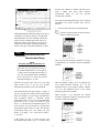
Introduction
WINDAQ/Lite waveform recording software can be
used with any Dataq Instruments hardware product.
It allows you to record waveforms directly and
continuously to disk while monitoring a real time
display of the waveforms on your computer screen.
It operates at the full sample rate of the instrument
being used (allowing you to see a real time display
of your waveform signals on your computer’s
monitor at the instruments full sample rate), but is
limited to 240 Hz maximum throughput when you
enter the record mode.
This manual contains information designed to
familiarize you with the features and functions of
the following serial port data recording modules:
DI-151RS
DI-195B
and also with WINDAQ/Lite waveform recording
software and WINDAQ Waveform Browser playback
and analysis software.
WINDAQ Waveform Browser allows you to review,
measure,
analyze,
compress,
cut-and-paste,
export/import, and otherwise manipulate the
recorded waveform information. It is available for
download free-of-charge from our web site
(www.dataq.com).
DI-151RS
The DI-151RS is a portable, two-channel data
recording module that communicates through your
computer’s RS-232 (or serial) port. It can record
data at rates up to 240 samples per second with 12bits of measurement accuracy.
Conventions Used in the Documentation
Before you start using the DI-151RS, DI-195B,
WINDAQ/Lite, or WINDAQ Waveform Browser
software, it’s important to understand the terms and
notational conventions used in this documentation.
The DI-151RS is powered directly from the
computer to which it is connected (through the RS232 cable).
The DI-151RS is equipped with a dedicated
thermistor input, two digital inputs, and two singleended, bipolar analog input channels.
General Conventions
Commands you choose are given with the menu
name preceding the command name. For example,
the phrase “Choose File Open” tells you to choose
the Open command from the File menu. This
naming convention describes the sequence you
follow in choosing a command — first you select
the menu, then you choose the command.
DI-195B
The DI-195B is a two-channel data recording
module that communicates through your computer’s
RS-232 (or serial) port. It can record data at rates up
to 240 samples per second with 12-bits of
measurement accuracy.
Mouse Conventions
In general, most mouse actions require only the left
mouse button. For example, carrying out a menu
command or working in a dialog box requires only
the left mouse button. However, the right mouse
button is not totally neglected. Among other things,
the right mouse button is used for copying waveform
data to the clipboard, waveform scaling, selecting a
waveform channel, etc.
The DI-195B is powered by the included wall outlettype adapter, which can be plugged into any singlephase, 120 volt, 60 Hz. AC source. It features two,
signal-conditioned, differential, bipolar analog
inputs
(screw
terminal
access,
maximum
measurement range is defined by the DI-5B
modules). The DI-195B allows you to plug any two
DI-5B signal conditioning modules into its
backplane. The DI-5B signal conditioning modules
then filter, isolate, amplify, and/or convert virtually
any industrial signal that is applied into a high level
analog voltage, perfectly suited for recording.
Since the majority of mouse procedures are done
with the left mouse button, we will not specify
which mouse button to click, drag, or double-click
with in the procedures unless it is the RIGHT
mouse button. When the right mouse button is
required, it will be specified as such. For example,
“Double-click the right mouse button anywhere in
the bottom annotation line to move the cursor to the
WINDAQ/Lite Waveform Recording Software and
WINDAQ Waveform Browser Playback and
Analysis Software
The WINDAQ software shipped with all of the serial
port instruments consists of WINDAQ/Lite waveform
1
selected from the File menu. RECORD is used to
stream waveform information to disk. While in this
mode, all waveform recording features and functions
are available (with some restrictions) except the
following: all channel-specific operations (i.e.,
channel number, gain, offset); and sample rate
adjustments. In this mode, waveform information is
being continuously streamed to disk while the real
time display remains active. In this mode, sample
rate is limited to 240 Hz maximum throughput,
regardless of the instrument being used. When in
this mode, the Status: area of the bottom annotation
line displays RECORD.
lowest displayed waveform valley.” When not
specified, the left mouse button is assumed for the
procedure.
• “Point” means to position the mouse pointer
until the tip of the pointer rests on what you
want to point to on the screen. For example,
“Point to the View menu.”
• “Click” means to press and immediately
release the mouse button without moving the
mouse. For example, “To display the menu
that contains the command you want, click the
menu name in the menu bar.”
The STANDBY operating mode becomes active
when waveform recording to disk is temporarily
suspended by choosing the Stop command from the
File menu. While in this operating mode, all
waveform recording features and functions are
available except: channel-specific operations (i.e.,
channel number, offset, etc.) and sample rate
adjustments. In this mode only the real time display
is active, waveform recording to disk has been
stopped. When in this mode, the Status: area of the
bottom annotation line displays STBY. It is possible
to start and stop the recording process as many times
as you like during a data acquisition session.
• “Double-click” means to click the mouse
button twice in rapid succession. For example,
“Double-click the icon to start the program.”
• “Drag” means to press the mouse button and
hold it down while you move the mouse; then
release the button. For example, “Drag down
to Data Cursor to enabled the cursor for onscreen display.”
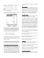
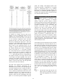
WINDAQ/Lite Operating Modes
WINDAQ/Lite waveform recording software has
three operating modes. They are, in logical order of
occurrence; Setup, Record, and Standby. Each
operating mode shares many features with the other
three, but there are some features accessible only
from one given mode. The three modes are
discussed in detail as follows:
The SET UP operating mode is active when
WINDAQ/Lite is first started. SET UP is used to
configure data acquisition parameters such as the
number of acquired channels, channel gain, and
channel offset. In addition, this mode is used to
adjust the real time display for a visually pleasing
presentation. Virtually all other data acquisition
functions and adjustments are available from the
SET UP operating mode including control of the real
time display screen’s scaling and offset functions. In
this mode only the real time display is active, data is
not yet being streamed (or stored) to disk. In this
mode, sample rate is limited only by the capabilities
of the hardware. In other words, you can sample as
fast as your instrument will allow. When in this
mode, the Status: area of the bottom annotation line
displays SET-UP.
The RECORD operating mode is active when a file
has been opened and the Record command has been
2
Getting Started
If you have an instrument other
than the DI-151RS or DI-195B and
you have not installed it yet, do so
now. Ignore the following steps
and proceed instead with the
installation instructions contained
in your hardware User’s Manual.
The following items are included with each
instrument purchase. Verify that you have the
following:
• DI-151RS, or DI-195B instrument.
DI-151RS and DI-195B Only
• Communications cable designed to connect the
instrument to your computer’s serial port (with the
DI-195B, the AC power adapter is integrated into
the serial cable).
• WINDAQ software diskette(s). We are currently
shipping both WINDAQ/Lite and WINDAQ
Waveform Browser software all on one disk.
However that may change at any time, in which
case you will have two diskettes.
• This user’s manual, which covers the hardware
aspects of the DI-151RS, and DI-195B serial port
modules and also documents WINDAQ/Lite
waveform recording software and WINDAQ
Waveform Browser playback and analysis
software.
1.
Connect the male end of the communications
cable to the 9-pin female connector on the DI151RS or DI-195B module.
2.
Connect the other end of the communications
cable to your computer’s serial or COM port.
3.
If you purchased the DI-195B, plug the AC
power adapter into any standard 120V, 60Hz
wall outlet.
Step 2
Installing WINDAQ
Software
NOTE
WINDAQ/Lite waveform recording
software and WINDAQ Waveform
Browser playback and analysis
software are both on the WINDAQ
Resource CD, but they must be
installed individually with separate
installation
procedures.
The
following procedure will install
WINDAQ/Lite recording software
first, then WINDAQ Waveform
Browser playback and analysis
software.
• If you purchased a DI-195B, you should also have
one or two DI-5B plug-in modules. Note that
these are extra-cost items not included with the
purchase of the DI-195B kit, but are required for
operation.
If an item is missing or damaged, call Dataq
Instruments at (330) 668-1444. We will guide you
through the appropriate steps for replacing missing
or damaged items. Save the original packing
material in the unlikely event that your unit must,
for any reason, be sent back to Dataq Instruments.
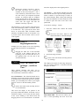
Step 1
Installing the Hardware
1.
Start Windows™.
2.
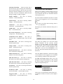
Insert the WINDAQ Resource CD into your CD
drive and close the drive tray.
For most user’s, the CD’s auto-run feature will
automatically display a list of options for you to
pick from. If you do not see this list of options
after a reasonable period of time, double-click
the My Computer icon on your desktop and then
double-click your CD-ROM icon to manually
display the list of options.
NOTE
Before
installing
WINDAQ
software, you should already have
the
hardware
installed
or
connected. If you have not done so
already, install or connect your
hardware at this time.
3.
Use the following procedure to
connect the DI-151RS, or DI-195B
module to your computer.
3
Choose the Install Software button and click
OK.
4.
Now choose the WINDAQ/Lite and Software
Development Kit button and click OK.
5.
Specify the instrument series (broad category)
that will be used with WINDAQ/Lite software.
If you have an instrument other
than the DI-151RS or DI-195B,
ignore the following steps and
proceed instead with the input
signal connection instructions
contained in your hardware User’s
Manual.
For example, choose the DI-1xx Serial
Data Acquisition Units button if you
have either the DI-151RS module or
the DI-195B module connected to your
serial port (both are 100 Series
instruments), or choose the DI-4xx
Series Plug-in Cards button if you
have a DI-400, DI-401, or DI-410
board installed, etc.
To connect signals to the DI-151RS or DI-195B,
insert the stripped end of a signal lead into the
desired terminal directly under the screw. Tighten
the pressure flap by rotating the screw clockwise
with a small screwdriver. Make sure that the
pressure flap tightens only against the signal wire
and not the wire insulation. Do not overtighten. Tug
gently on the signal lead to ensure that it is firmly
secured.
When the instrument series button is
selected, click the OK button.
6.
The remaining installation steps vary by
instrument. In most cases, the on-screen
prompts provide enough information to
successfully get you through the installation.
However, if you are unsure of what to do next
or if you need additional information, contact
Dataq Instruments technical support.
7.
When WINDAQ/Lite software has successfully
been installed, double-click the My Computer
icon on your desktop and then double-click your
CD-ROM icon to manually display the list of
installation options.
8.
Again choose the Install Software button and
click OK.
9.
Select the WINDAQ Waveform Browser button
and click OK to install WINDAQ Waveform
Browser playback and analysis software. The
on-screen prompts should provide enough
information to successfully get you through the
installation. However, if you need additional
information, contact Dataq Instruments
technical support.
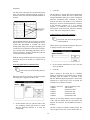
DI-151RS
All user connections are made to the 8-port screw
terminal connector as follows:
Ch 1: Channel 1 signal input.
Gnd: Channel 1 signal ground.
Therm 1: Thermistor lead 1 input.
Therm 2: Thermistor lead 2 input.
Dig 0: Digital input 0.
Dig 1: Digital input 1.
Step 3
Gnd: Channel 2 signal ground.
Connecting Your Input
Signals to the Instrument
Ch 2: Channel 2 signal input.
Your DI-151RS comes with the on-board waveform
generator configured to provide a sample input
signal. The onboard waveform generator is enabled
by connecting a jumper wire between the Ch 1 and
Dig 1 inputs. A thermistor is also included for
temperature measurements. So it doesn’t get lost
during shipping, one leg of the thermistor is
NOTE
Use the following procedure to
connect your input signals to the
DI-151RS or DI-195B module.
4
signal to be measured is ground-referenced, or the
signal to be measured is isolated from ground. In
either case, it is important to properly connect the
differential amplifier.
connected to a screw terminal. Unless you would
like to make temperature measurements with the
thermistor, remove it completely from the DI151RS. Do not make voltage measurements with the
thermistor installed. Any voltage measurement made
with the thermistor installed will be inaccurate.
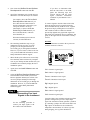
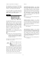
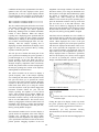
Ground Referenced Signal Sources — A ground
referenced signal source is one with a local ground
that may not be (and probably is not) at the same
potential as the computer’s ground. This potential
difference between signal ground and computer
ground is referred to as a common mode voltage and
is caused by a number of different factors.
When using the termistor to make temperature
measurements, insert one thermistor leg into input
Therm 1 and the other thermistor leg into Therm 2.
In order to get accurate temperature measurements,
the thermistor must be calibrated. The procedure for
doing this is included in step 8.
signal
source
When the DI-151RS is configured for voltage
measurements, Ch 1 and its Gnd make up one
single-ended analog input channel, while Ch 2 and
its Gnd make up the other.
DI-195B
All user connections are made to the two, four-port
screw terminal connectors.
computer
ground
ground potential difference
(common mode voltage)
The most common of these is different physical
locations of the computer and signal ground points.
Since wire is not a perfect conductor (i.e., exhibiting
zero resistance regardless of length) a voltage drop,
however small, will always be present. The
differential amplifier is unique in its ability to
measure signals originating from sources with
different ground potentials relative to the computer
providing it is connected properly.
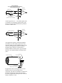
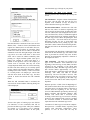
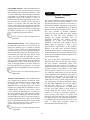
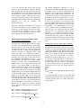
WRONG APPROACH!
Circulating currents in signal shield induce
noise on signal of interest.
IN+ and IN- are the signal input terminals for each
channel. EX+ and EX- are excitation voltage
outputs for those transducers that require excitation.
Obviously, you’ll want to tailor the DI-5B signal
conditioning modules used in the instrument to the
kind of input signals you wish to record.
instrument
input terminals
signal source
signal
lead
shield
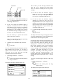
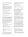
Differential Inputs
DI-195B features two dedicated differential input
channels. Differential input channels respond only to
the difference in voltage between each (+) and (-)
analog input, effectively suppressing common mode
voltages (i.e., identical voltages appearing
simultaneously and in phase on both inputs). Since
most forms of interference or noise are applied with
equal intensity to both inputs of a differential
amplifier (that is, in the common mode), the
differential amplifier is very effective at rejecting
noise riding on a signal of interest.
differential
amplifier
gnd
Ground loop
caused by
circulating currents
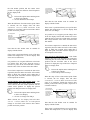
The most common error made in connecting
differential amplifiers is the tendency to ground both
ends of a signal shield. This causes current to flow
through the shield and induces noise on the signal to
be measured. This problem is eliminated by
ensuring that only one ground exists on the signal
circuit.
Two types of signal sources are likely to be
encountered when configuring your DI-195B; the
5
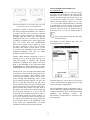
RIGHT APPROACH √
One ground on the signal circuit eliminates
noise-inducing ground loops
instrument
input terminals
signal source
signal
lead
shield
differential
amplifier
gnd
Potential difference
(no path for current to circulate)
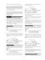
Isolated Signal Sources — An isolated signal source
is one that is not connected to ground at any point.
However the signal shield should still be grounded
as before to reduce noise.
instrument
input terminals
Floating signal source
signal
lead
shield
differential
amplifier
gnd
Any application requiring a differential amplifier
also defines a need for quality signal cable. Four
elements combine to ensure adequate quality signal
cable; a twisted signal pair with low resistance
stranded copper conductors, surrounded by a
multiple-folded foil shield, with a copper stranded
drain wire, all contained within an insulated outer
jacket.
Drain wire
Insulated outer jacket
Foil shield
Twisted signal pair
Stranded copper conductors
In applications where such signal cable is used, a
dramatic decrease in noise pickup will be
experienced. The drain wire should be considered as
the shield and should be connected as described
previously. Signal cable meeting all four criteria for
quality is Belden No. 8641.
6
Fast Start to
Recording
Waveforms
with
WINDAQ/Lite
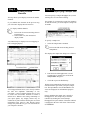
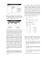
Point to the Edit menu and drag down to
Channels…
This causes the Ch: block cursor to blink in the
Channels: field on the status bar. The currently
active list of enabled channels are displayed in this
field, immediately to the left of the cursor (initially,
only channel 1 is enabled for recording).
2.
After you have completed all hardware and software
installations and connected your signals, you are
ready to record.
A single-ended channel is added to the list by
entering the channel’s number and pressing the
ENTER key.
Steps 4 through 9 below outline the “fast start”
procedure for recording waveforms to disk. These
are the basic steps you will take every time you
record with WINDAQ/Lite waveform recording
software.
A differential channel is added to the list by
entering the channel’s number followed by the
letter “D” (e.g., “3D”) and pressing the ENTER
key.
The rest of this chapter contains additional recording
functions that will not necessarily be used in every
session or are not requisite for recording, but will
make future recording sessions easier. After your
initial, “get-acquainted” recording session, take a
few moments and look over these functions.
This causes the channel number to be displayed in
the enabled channels row.
3.
Disable channel configuration by pressing any
key other than the letters “D” and “I”.
Note that a channel may be removed by typing the
channel number preceded by a minus (“-”) sign.
Make sure that you use the minus sign on the main
keyboard, not the minus sign that resides on the
keypad (the minus sign on the keypad performs an
entirely different function). For example, typing “1” removes channel 1 from the row. Note also that it
is not possible to remove all the channels from the
row (in other words, have no channels enabled). For
example, say you are using the DI-195B and you
have only channel 1 configured and it is a
differential channel (Channels: field reads “1D”).
Typing “-1D” will not remove it from the row.
Typing “1” will however, change it to a singleended channel, and vice-versa.
Step 4
Enabling Channels for
Acquisition
It is assumed at this point that you have
WINDAQ/Lite waveform recording software running.
If not, click the Start button on the taskbar, point to
Programs, point to WINDAQ (or whatever you
named the group window during step 11 of the
installation), and click WinDaq Acq.
This step specifies which analog channels to record.
For example, suppose we have analog signals
connected to channels 1 and 2, and we want to
record both of them. Use this procedure to enable
channels 1 and 2 for recording:
1.
Enter the desired channel number and press the
ENTER key. Repeat for each desired channel.
Channels may not be added after the RECORD
mode has been entered.
To enable channel configuration:
7
Step 5
Step 6
Viewing Enabled
Channels
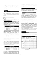
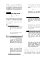
Specifying a Sample Rate
You must specify a sample throughput rate (or total
scanning rate) for waveform recording.
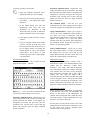
This step allows you to display onscreen all enabled
channels.
For example, if you wanted to acquire four channels
of data all at 60 Hz, you would require a sample rate
of 240 Hz.
If you enabled more channels in the previous step,
you will want to display them all onscreen.
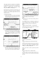
1.
To display enabled channels:
1. Point to the View menu and drag down to
Format Screen.
2. In the format box, click the desired
display format.
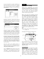
To specify a sample rate:
Any channel may be displayed as an overlapping or
non-overlapping display.
1.
Select the Sample Rate command:
Point to the Edit menu and drag down to
Sample Rate…
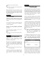
This displays the sample rate dialog box as follows:
2.
Enter the desired throughput rate (or total
scanning rate) in samples per second in the
Sample Rate dialog box.
3.
Click OK or press the ENTER key.
WINDAQ/Lite automatically allocates the correct
amount of buffer space when you input a sample
rate. The Input Buffer Size and Disk Buffer Size
values are displayed for informational purposes
only.
An overlapped format allows you to closely examine
the time and amplitude relationship of two
waveforms. A non-overlapped format may be used
to isolate each waveform’s transition to within a
defined area. Whatever the timing relationship of
your input signals, any display format may be
enabled at any time without affecting the waveform
information being stored to disk. Display format
changes only affect the way you view waveforms on
your computer’s monitor.
Keep in mind that the sample rate is actually a
throughput rate. The sample rate per channel
(obtained by dividing the selected sample
throughput rate by the number of channels enabled)
is displayed in the lower left corner of the window
as S/s/CHAN:.
8
skip this step. Otherwise, continue with this step to
select a higher gain factor (thus narrower
measurement range) for the best possible
measurement resolution.
Since gain and measurement range can be assigned
per-channel, the desired channel must first be
selected.
1.
Select an analog channel for gain adjustment:
Click the left mouse button in the unselected
channel’s annotation margin.
Although thousands of different sample rates may be
configured, some discrete rates are not achievable.
This limitation is due to the inability to divide the
master clock in a manner that results in an evennumbered quotient. For example, say you enter a
sample rate of 200. What you might actually get,
because of the previously stated limitation, is 200.3.
Step 7
Specifying Gain and
Measurement Range
The focal point for selecting a channel for any type
of adjustment is the variable waveform assignment
indicator.
NOTE
DI-151RS, DI-195B, and DI-401 Users
DI-151RS, DI-195B and DI-401 users can
ignore this step and proceed with step 8.
DI-151RS instruments have a fixed gain of
1 (unity) and a fixed measurement range of
±10 volts. DI-195B and DI-401 instruments
have a fixed gain of 1 (unity) and a fixed
measurement range of ±5 volts.
This two-element equality (X=Y) is displayed for
every enabled channel. Element “X” (1 in the
illustration above) is the window number. Element
“Y” (0 in the illustration above) is the analog
channel assigned to that window.
Choosing the proper gain factor for your input
signals allows you to get the best possible
measurement resolution out of your instrument.
The default WINDAQ/Lite gain setting is 1 (unity). A
gain of 1 provides the widest possible measurement
range. For example, say you’re using a DI-400-PGH.
This instrument features a maximum analog
measurement range of ±10 volts and programmable
gain factors of 1, 2, 4, and 8. At a gain of 1 (gain
factor = 1), the full scale measurement range is ±10
volts. However, if we set the gain to 2, the full scale
measurement range becomes ±5 volts. The full scale
measurement range gets even smaller for gain
factors of 4 (range = ±2.5 volts) and 8 (range =
±1.25 volts).
When selected, a box surrounds the variable
waveform assignment indicator, indicating that the
window is enabled for adjustment.
If the signals you plan to record need the wide
measurement range that a gain of 1 provides, then
9
leave the Unipolar box unchecked, thus specifying
bipolar.
When the desired channel is selected, gain
adjustments to that channel are now possible.
2.
Reset Cal. Button
Whenever the gain or unipolar/bipolar setting is
changed, any calibration is preserved and adjusted to
reflect the new gain or unipolar/bipolar setting.
Selecting Reset Cal allows you to reset the selected
channel from a significant engineering units
calibration back to the default voltage (or
temperature, if using thermocouples) calibration.
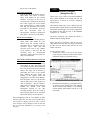
Select the Channel Settings… command:
Point to the Edit menu and drag down to
Channel Settings…
This displays the “Channel X Settings” dialog box
(where X represents the enabled channel):
Acquisition Method
Allows you to select the method used for recording
and displaying data (intelligent oversampling).
All Dataq Instruments hardware products
continuously sample data using a burst sampling
technique. The hardware samples data at one rate
(referred to as the burst rate) while your computer
reports (i.e., displays and stores) this data at another
rate (called the sample rate or throughput rate). For
example, let’s say we want to record one channel at
100 Hz and our burst rate is set at 50kHz. This
means that for every 500 data points sampled, only 1
will be reported. The dilemma becomes; which data
point out of the 500 gets reported? Fortunately, you
have a choice for reporting this single data point:
The gain factors you see displayed at the top of this
dialog box are hardware dependent. Displayed next
to each gain are the equivalent plus and minus full
scale voltages that result from selecting that gain
factor. These voltages vary by hardware device.
3.
Click on the desired gain factor.
4.
Click OK or press the ENTER key.
Average - Averages all of the data points in the burst
sample and reports this average as the single value
for storage and display.
Last Point - Reports the last input data point in the
burst sample, ignoring the rest.
Maximum - Reports the highest value data point in
the burst sample, ignoring the rest.
As the gain factor for a channel is sequenced upward
and downward through gain ranges, ±full scale
annotation adjusts to reflect the application of the
various gain factors.
Minimum - Reports the lowest value data point in
the burst sample, ignoring the rest.
A channel's gain factor cannot be adjusted following
the initiation of data storage to disk. Only the SETUP operating mode allows gain factor adjustments.
Input Types
Linear - The default setting, available on all
instruments, should be used with all linear inputs.
Unipolar/Bipolar Measurement Range Option
You can specify whether the signal you will be
acquiring is unipolar or bipolar. A unipolar signal is
one that ranges from 0 to + full scale (never goes
below zero), and a bipolar signal is one that ranges
from some negative value to some positive value (is
both positive and negative going). If your signal is
only a positive going waveform or a negative going
waveform, always select the Unipolar check box. If
your signal is both positive and negative going,
Thermocouple - Selectable only on instruments with
the hardware to support thermocouples.
Nonlinear - Also only on instruments that support
thermocouples. Used only with a specialized, nonlinear, non thermocouple type of sensor.
Next and Previous Buttons
Allow you to step through the next or previous
enabled channel (in order), setting up each channel
10
for gain, unipolar/bipolar, sample rate, etc., without
closing this dialog box.
To calibrate a waveform using this high/low
calibration method:
Step 8
1.
Calibrating Your Input
Signals
Select the window that contains the desired
waveform:
Click the left mouse button in the
unselected window’s annotation margin.
Calibration allows you to view and record your
waveform data in significant engineering units.
Without calibrating, waveform data is scaled,
annotated, and displayed in volts, which in many
cases is not very meaningful. Calibration is used to
give meaning to the displayed data. Instead of volts,
your data can be scaled, annotated, and displayed in
significant engineering units (i.e., PSI, RPM, lbs,
ft/s, etc.).
This function allows your waveform data to be
calibrated in significant engineering units using any
known or verified transducer output values.
For example, suppose you were acquiring pressure
data with a transducer that had a known output of -1
volt at 0 psi and 4.5 volts at 100 psi. Whether these
output levels were read from the manufacturers
specifications or verified through use, they can be
used as calibration values.
2.
If not already enabled, enable the Current Data
and Data Display options (on the Options
menu).
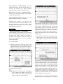
3.
Select Low Calibration… as follows:
Point to the Edit menu and drag down to
Low Calibration…
This displays the Low Calibration dialog box:
With this method, you can even calibrate the data
without knowing the transducer output relationship.
Simply let WINDAQ/Lite software establish these
output voltage values for you. For example, suppose
you were acquiring pressure data and you had no
idea what kind of output voltages to expect from the
transducer you’re using. You could vent the pressure
apparatus to quiescence or atmospheric pressure and
observe what voltage the transducer is outputting at
quiescence from the Input Level text box in the Low
Calibration dialog box (select Low Calibration…
from the Edit menu). In this same dialog box, enter
what you would like this quiescent state to be, such
as “0”, in the Low Cal Value text box, and enter
“PSI” in the Engr. Units text box. Now activate the
OK command button to close the dialog box, and
increase the pressure until the manometer reads a
convenient value, say 100 psi. In a similar manner,
observe what voltage the transducer is outputting at
this 100 psi level from the Input Level text box in
the High Calibration dialog box (select High
Calibration… from the Edit menu). Enter “100” in
the High Cal Value text box, enter “psi” in the
Engr. Units text box, choose the OK command
button, and you’re done.
This is where you enter the low calibration data
value that is to be assigned to the input voltage
level. For instance, referring back to our
previous examples:
a)
11
For the case where the transducer output is
known,
Input level
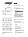
This is where you enter the high calibration data
value that is to be assigned to the input voltage
level. For instance, referring back to our previous
examples:
Cal value
Engr. units
-1 volt
at
0
PSI
4.5 volts
at
100
PSI
a)
we would enter “0” in the Low Cal Value text
box, “-1” in the Input Level text box, and “psi”
in the Engr. Units text box.
b) For the case where the transducer output is
unknown, we would also enter “100” in the
High Cal Value text box (after 100 psi has been
applied in our example), ignore the Input Level
text box (WINDAQ/Lite software has established
the input voltage level for you), and enter “psi”
in the Engr. Units text box.
b) For the case where the transducer output is
unknown, we would also enter “0” in the Low
Cal Value text box (with the test apparatus
vented to atmospheric pressure), ignore the
Input Level text box (WINDAQ/Lite software
has established the input voltage level for you),
and enter “psi” in the Engr. Units text box.
6.
The High Calibration dialog box disappears and the
waveform channel displays all waveform data values
calibrated in the chosen engineering units.
Type up to a four character optional engineering
unit tag (i.e., PSI, f/s, rpm, etc.).
If desired, the upper and lower grid limit values may
be specified (and the waveform automatically scaled
to fit). This feature allows the channel's full scale
display span to be shown in whole numbers rather
than obscure fractional values, which sometimes
result from calibrating. For example, a waveform
scaled in mmHg can be automatically expanded or
contracted to fit within grid limits of 0 to 100
mmHg, or -200 mmHg to +200 mmHg, or whatever
is desired. Note that a channel spanning 0 - 200
mmHg is much easier to read and interpret on a per
division basis than one that spans 10.372 - 189.628
mmHg.
Complete the low calibration entry as follows:
Click OK.
The Low Calibration dialog box disappears and if no
high calibration has been done yet, an offset is
applied to the waveform to achieve the entered
value. But you are only half done, the high
calibration value must also be entered.
5.
Complete the high calibration entry as follows:
Click OK.
Press the TAB key to position the insertion
point in the various text boxes.
4.
For the case where the transducer output is
known, we would enter “100” in the High Cal
Value text box, “4.5” in the Input Level text
box, and “psi” in the Engr. Units text box.
Select High Calibration… as follows:
To specify convenient upper and lower chart edge
values:
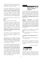
7. Select Scaling Limits… as follows:
Point to the Edit menu and drag down to
High Calibration….
This displays the High Calibration dialog box:
Point to the Scaling menu and drag
down to Limits….
This displays the Display Limits dialog box:
12
8.
Type convenient top and bottom chart-edge
values in their respective text boxes.
9.
Complete the chart-edge value entry as follows:
1.
Select the Record command:
Point to the File menu and drag down to
Record.
This displays the Open dialog box. Here is where
you specify a file name (to create a new file) or open
an existing file (to append to it).
Click OK.
Your specified values will now be displayed on the
upper and lower chart-edges and the waveform will
be automatically scaled to fit the new values.
If creating a new file, you will be prompted to
specify a maximum file size. If appending to an
existing file, you will be prompted to specify how
much additional data to add to the existing file.
The Next and Previous buttons allow you to step
through all of the enabled channels in order, entering
the desired display limits for each channel, without
closing this dialog box.
In either case, you can specify file size in kilobytes
or recording time. In the case of recording time, file
size is based on the currently selected sample rate.
Note that you can experiment with different file
sizes, sample rates, and recording time to get the
desired result. Move between the two text boxes
with the TAB key.
When using the DI-151RS, the following procedure
can be used to calibrate the thermistor transducer:
1. With the thermistor connected to the DI-151RS
as described in step 3 of this fast start
procedure, submerge the tip of the thermistor in
an ice water bath. Submerge only the tip of the
thermistor, do not submerge the DI-151RS. Let
it remain in the ice water long enough for the
thermistor output to stabilize (you can monitor
the thermistor output with WINDAQ/Lite’s real
time display).
2.
Enter the desired file size or accept the default.
3.
Close the dialog box and begin recording by
clicking OK or pressing the ENTER key.
When you enter the desired file size or accept the
default, you are placed in the active record-to-disk
operating mode where enabled analog channel data
is simultaneously digitized, displayed, and streamed
to disk. The status field in the bottom annotation
line indicates RECORD.
2. Follow steps 1 through 4 of the calibration
procedure described above, but enter “32” in the
Low Cal Value text box, and “F” in the Engr.
Units text box. Note that WINDAQ/Lite has
established the Input Level value automatically.
3. Now remove the thermistor from the ice water
bath and allow it to stabilize at room
temperature.
4. Follow steps 5 through 9 above, but enter “72”
(or whatever your room temperature is) in the
High Cal Value text box, and “F” in the Engr.
Units text box. For convenient display limit
values, enter “100” in the Top Limit text box
and “0” in the Bottom Limit text box.
Step 9
To stop acquisition to disk:
Recording Waveforms to
Disk
Point to the File menu and drag down to
Stop.
The Record function on the File menu initiates
recording to disk. To begin waveform recording:
13
cut and paste portions of waveforms, and do all
forms of interpretive analysis, launch the WINDAQ
Waveform Browser by clicking or double-clicking
on the WINDAQ Waveform Browser icon (created
during installation). Then refer to the section of this
manual titled “Reviewing Recorded Waveforms
with WINDAQ Waveform Browser” for complete
details.
This suspends data storage to disk, but the real time
display remains active. The status field in the
bottom annotation line indicates STBY when
acquisition has been stopped. The Stop function on
the File menu only becomes selectable when in the
record-to-disk mode.
As data is being recorded to disk, the amount of file
space consumed is displayed in the “Storage:” field
of the status bar as a percentage of total file space
consumed.
Data acquisition to disk may be started and stopped
as many times as desired. When the target data file
has been filled, data acquisition to disk will cease,
the “Storage:” field of the status bar will display
“100% used”, and the “Status” field of the status bar
will display FILE FULL.
Each time recording is activated, an event marker is
automatically inserted in the data stream. This
allows acquisition break points to be reviewed using
WINDAQ Waveform Browser playback and analysis
software.
This concludes the “fast start” procedure for
recording waveforms to disk. The next logical step
is to review the data you just recorded. This is done
with WINDAQ Waveform Browser playback and
analysis software (WWB). To make timing and
amplitude measurements, review event markers,
overlap waveforms to examine interdependencies,
14
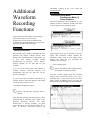
periodically pointing to the View menu and
selecting Refresh.
Additional
Waveform
Recording
Functions
WINDAQ/Lite
Scroll Mode,
Oscilloscope Mode, &
Pause Graphics
Waveform information can be displayed on your
monitor in either a continuous smooth scroll mode
or in a triggered sweep oscilloscope mode.
These functions are not requisite for recording or
will not necessarily be used every time
WINDAQ/Lite is used, but are included to make
recording easier and more productive, or to increase
display performance and visual appeal.
WINDAQ/Lite
Browse
This function starts WINDAQ Waveform Browser
playback and analysis software directly from
WINDAQ/Lite recording software. This enables you
to have both software packages running
simultaneously to playback, review, analyze,
measure, quantify, etc. the data that was just
recorded.
Either display mode may be enabled at any time
during data acquisition without affecting the
information being stored to disk. Display mode
changes only affect the way waveforms are
displayed on your monitor.
If you are in the record mode when Browse is
selected, WINDAQ Waveform Browser will
automatically open the very same file you are
actively recording to.
Point to the Options menu and drag down to
Scroll Mode or Oscilloscope Mode…
1.
Select a display mode:
Note that in either display mode, the waveform
display can be paused. This allows you to get a
stationary look at some point on the waveform.
While paused, the Mode: field in the status bar
changes from the chosen display mode to Paused.
If you are not in the record mode when Browse is
selected, WINDAQ Waveform Browser will prompt
you for the file you wish to review.
To enable this multitasking feature:
Point to the File menu and drag down to
Browse.
This starts the WINDAQ Waveform Browser. Since
waveform data is constantly being written to this
Waveform
Browser
file
while
WINDAQ
WINDAQ/Lite is actively recording, you must
request updates to see all of the latest data. This is
done in WINDAQ Waveform Browser by
15
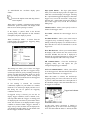
Slope option buttons - The slope option buttons
allow you to select the slope (positive or negative) at
which the waveform display will trigger. Selecting
the + option button triggers the display to start at the
trigger level, but on the waveform’s rising slope.
Selecting the - option button triggers the display to
start at the trigger level, but on the waveform’s
falling slope.
To enable/disable the waveform display pause
feature:
Point to the Options menu and drag down to
Pause Graphics.
When pause is enabled, a subsequent pause attempt
disables the paused waveform. The display mode
that was active before pausing is restored.
Channel text box - Allows you to specify or select a
channel for the trigger source.
If the display is paused while in the Record
operating mode, data acquisition to disk continues
unimpeded, only the display is paused.
Level field - Indicates the current trigger level in
volts.
Free Run check box - Allows you to select between
a triggered sweep oscilloscope display or a freerunning oscilloscope display (see discussion above).
Note that this box must be unchecked to set the
trigger level.
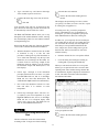
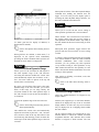
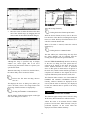
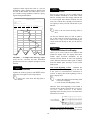
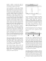
When Oscilloscope Mode… is chosen from the
Options menu, the Oscilloscope Triggering dialog
box is displayed as follows:
Erase Bar check box - Allows you to enable/disable
the display of the vertical erase bar (cursor) on the
waveform. Whether the erase bar is displayed or
disabled, the waveform information on screen is still
“erased” and replaced with a fresh sweep of data.
OK command button - Closes the Oscilloscope
Triggering dialog box and applies the just
configured display trigger conditions.
This dialog box allows you to select one trigger
channel and display the data in a triggered sweep
oscilloscope format or in a free-running oscilloscope
format. Checking the Free Run check box selects
the free running oscilloscope format. Leaving the
Free Run check box unchecked selects the triggered
sweep oscilloscope format.
Set Level command button - Allows you to adjust
or set the trigger level. Note that the Free Run check
box must be unchecked to set a trigger level.
When this button is selected, the Oscilloscope
Triggering dialog box closes and causes the cursor
to point to a short horizontal line at the right side of
the annotation margin. This short horizontal line is
the trigger level indicator.
If free running is selected, the waveform
continuously updates on your monitor in a manner
identical to an oscilloscope display and the rest of
this dialog box can be ignored (no triggering
conditions need be set).
Trigger level indicator
If triggered sweep is selected, you can also set
display trigger conditions (such as channel, level,
and slope) that define the “trigger” or starting point
for displaying the waveform on your monitor. In this
mode, the waveform is not displayed until a trigger
condition is detected. When a trigger is detected, a
single sweep of the waveform will be displayed on
your monitor and will remain on your monitor until
the next trigger condition is detected.
At this point, mouse movement is limited to
dragging the line up or down to the desired trigger
level. Note that when the mouse is moved, the data
16
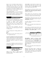
Current Data - Enables/disables the display of the
current waveform data value in the left or right
annotation margin. The Data Display option must
first be enabled for this option to work.
display in the left annotation margin changes to
indicate trigger level. When set where desired,
clicking the left mouse button sets a new trigger
level while clicking the right mouse button retains
the existing level. Note that if the trigger level is set
somewhere above or below the current signal, the
signal will disappear from the display.
When enabled in the oscilloscope mode, the current
waveform data value at the cursor position is
displayed in the annotation margin (the cursor does
not have to be enabled).
Cancel command button - Closes the Oscilloscope
Triggering dialog box and cancels any changes
made to trigger conditions (provided the changes
were not saved with the OK command button).
When enabled in the scroll mode, the current
waveform data value at the real time point (far right
screen edge) is displayed in the annotation margin.
WINDAQ/Lite
When disabled (in either mode), the base line value
is displayed in the left/right annotation margin (if
Data Display is enabled).
Open Reference File
Allows you to use an existing data file as a “set up”
for a new data file. All recording parameters (such
as number of channels, scaling constants,
engineering units, display format, compression,
display mode, gain, etc.) are ported from the
existing file to become the default conditions for the
new data file.
To enable current waveform data (if disabled, or
disable it if enabled):
Point to the Options menu and drag down to
Current Data.
This function allows instantaneous setup, thus
making it easy to run similar but separate waveform
recording sessions.
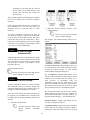
When enabled, the annotation margin will have the
following appearance and a check mark (√) will be
displayed on the Options menu immediately
preceding the Current Data command:
To use an existing file’s recording parameters for a
new file:
Data cursor
(vertical line)
Current waveform
value at cursor position
Point to the File menu and drag down to
Open Reference File…
Current data enabled (shown in oscilloscope mode)
You will be prompted for the name of the existing
data file. This file must be one created by WINDAQ
software and must already exist. When a filename is
entered and the dialog box is closed, the new file
immediately inherits the existing file’s recording
parameters.
Data Display - Displays or hides the current
waveform data value (or the baseline value,
depending on the state of the Current Data option)
in the annotation margin. If Limit Display is not
enabled, the engineering units will toggle on and off
along with the value. To display data (if hidden, or
hide it if displayed):
This function is enabled only when in the SET-UP
operating mode (Status: field in bottom annotation
line indicates SET-UP).
Point to the Options menu and drag down to
Data Display.
WINDAQ/Lite
Current Data, Data
Display, Limit Display &
User Annotation
When the data display option is enabled, the
annotation margin will have the following
appearance and a check mark (√) will be displayed
on the Options menu immediately preceding the
Data Display command:
Allows you to enable or disable on-screen
annotation options. Each annotation option is
described as follows:
17
WINDAQ/Lite
Data display enabled
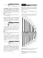
ToolBox
When enabled, a floating “toolbox” of buttons is
displayed on your screen. The toolbox buttons
provide quick access to commonly used commands.
To display the toolbox:
Limit Display - Displays or hides the upper and
lower chart-edge limits in the left/right annotation
margin. If Data Display is disabled, engineering
units toggle on and off along with the limits. To
display upper and lower chart-edge limits (if hidden,
or hide them if displayed):
Point to the View menu and drag down to
ToolBox.
Each button on the ToolBox provides quick access
(a shortcut) to commonly used functions as follows:
Point to the Options menu and drag down to
Limit Display.
Open reference file
When the limit display option is enabled, the
annotation margin will have the following
appearance and a check mark (√) will be displayed
on the Options menu immediately preceding the
Limit Display command:
Open/close file
Start/stop recording
Enable channels
Channel setup
Calibration
Limit display enabled
Sample rate
User Annotation - Toggles the display of user
annotation (entered from the Edit menu, User
Annotation… command) in the waveform strip. To
display user annotation (if hidden, or hide it if
displayed):
Waveform
compression
Commented
event
marker
Point to the Options menu and drag down to
User Annotation.
When user annotation is enabled, the waveform strip
will display the specified channel’s annotation
(entered with Edit User Annotation…) and a check
mark (√) will be displayed on the Options menu
immediately preceding the User Annotation
command:
Trigger
mode
Oscilloscope
mode
Scroll mode
Shift waveform down
User annotation enabled
Shift waveform up
Shrink waveform 2x
Expand waveform 2x
Screen annotation options can be enabled in
virtually any combination to provide the desired
result. However, in some instances one option will
override another. For example, if Data Display is
disabled, it is not possible to enable Current Data.
Similarly, if Limit Display is disabled, it is not
possible to enable Current Data.
Change palette
Show/hide grid
Open Reference File — The same as choosing
Open Reference File… from the File menu.
Open/Close File — The same as choosing Open…
from the File menu or, when a file is already open,
closes the file.
18
Start/Stop Recording — When activated with a
data file already open, recording starts immediately.
When activated without a data file open, the Open
dialog box appears prompting you to specify a new
file name or select an existing file. When activated
during recording, recording is stopped.
WINDAQ/Lite
User Annotation…
Allows you to display a custom message (up to 30
characters) on the baseline of each display channel
(used in tandem with the User Annotation function
on the Options menu).
Enable Channels — The same as choosing
Channels… from the Edit menu.
The desired channel annotation must first be entered
before it can be toggled on or off. To enter channel
annotation:
Channel Setup — The same as choosing Channel
Settings… from the Edit menu.
Point to the Edit menu and drag down to
User Annotation…
Calibration — The same as choosing Fixed
Calibration… from the Edit menu.
This displays the Channel Annotation dialog box as
follows:
Sample Rate — The same as choosing Sample
Rate… from the Edit menu.
Waveform Compression — The same as choosing
Compression… from the Edit menu.
Commented Event Marker — The same as
choosing Insert Commented Mark from the Edit
menu.
This dialog box prompts you to enter the desired
channel annotation for the currently selected
channel, or any other channel. If not the currently
selected channel, enter the desired channel number
for which you want to provide annotation in the
Channel # = text box. In the Annotation = text
box, enter the desired channel annotation (up to 30
characters).
Show/Hide Grid — The same as choosing Grids
from the Options menu.
Change Palette — The same as choosing User
Palette… from the File menu.
Expand Waveform 2X — The same as choosing
Grow 2X from the Scaling menu.
Once the channel annotation is entered, the display
of user annotation can be toggled on or off with the
User Annotation command on the Options menu.
Shrink Waveform 2X — The same as choosing
Shrink 2X from the Scaling menu.
Shift Waveform Up — The same as choosing
Waveform Up 10 Pixels from the Scaling menu.
The Next and Previous buttons allow you to step
through all of the enabled channels in order, entering
the desired channel annotation for each channel,
without closing this dialog box.
Shift Waveform Down — The same as choosing
Waveform Down 10 Pixels from the Scaling menu.
Scroll Mode — The same as choosing Scroll Mode
from the Options menu.
WINDAQ/Lite
Compression…,
Compression x2,
Compression /2
Oscilloscope Mode — The same as choosing
Oscilloscope Mode… from the Options menu.
Allows you to vary the number of data points used
to display the real time waveform on your computer
screen.
Triggered Mode — The same as choosing
Triggered Mode… from the Options menu.
19
Point to the Edit menu and drag down to
Compression x2.
To divide the current compression factor by 2:
Point to the Edit menu and drag down to
Compression /2.
This function is simply a “graphics adjuster” that
only affects how the display looks on your screen.
Data acquisition is independent of this function and
is always recorded (gap-free) at a compression factor
of 1 (no compression applied).
Perhaps these two functions are most useful when
the accelerator keys (PGUP for Compression x2 and
PGDN for Compression /2) are used. This allows
you to press one key several times in succession to
find just the right amount of compression for a
smooth scrolling, visually pleasing display.
When compression is applied to the waveform,
multiple A-D readings (equal to the compression
factor) are evaluated for plotting. In this instance,
less CPU time is required for the display. For
example, if compression equals 100, then 100
consecutive A-D readings are evaluated to define a
waveform point.
As the waveform compression factor is changed, the
time base field (ms /DIV: or sec /DIV:) displayed in
the bottom annotation line is automatically adjusted
to reflect the proper time scaling of displayed
waveforms.
When compression is selected, a true min/max is
performed on the waveform to ensure that transient
information is always displayed.
WINDAQ/Lite
Time Base
The degree of waveform compression is controlled
as follows:
Displays the time per major division at the bottom of
the real time screen as sec / DIV: or ms / DIV:. The
displayed value is a function of the selected sample
rate, the number of channels enabled, and the
selected waveform compression factor.
Point to the Edit menu and drag down to
Compression…
This displays the Compression dialog box as
follows:
To specify a degree of waveform compression:
Enter the desired compression factor (from 1
to 65,536) and click OK.
Time per major division
Time per major division is displayed at all times in
all operating modes.
A fast and convenient way to experiment with many
different compression factors is with the
Compression x2 and Compression /2 commands.
These commands respectively multiply or divide the
current compression factor by 2.
WINDAQ/Lite
Beep on File Full
When enabled, this option sounds an audible beep
when the target file is full.
To multiply the current compression factor by 2:
20
To enable the beep on file full function:
WINDAQ/Lite
Insert Mark, Insert
Commented Mark
Point to the Options menu and drag down to
Beep on File Full.
This function allows you to insert event markers
(either commented or uncommented) at any point in
the data stream going to disk. Event markers (along
with appropriate comments) can be used to mark an
event, or flag an uncommon occurrence in the data
stream going to disk, thus providing a complete
record of what happened and why.
When enough data has been recorded to fill the
allocated file space, an audible beep sounds (when
this function is enabled) to warn you that acquisition
has stopped and WINDAQ/Lite software is in the
STBY operating mode.
WINDAQ/Lite
After the waveform recording session, WINDAQ
Waveform Browser playback software allows you to
automatically search and move to the point in the
data file where the event markers were placed
during data acquisition.
Close
Allows you to close the data file you are currently
working with. Closing a data file removes the file
from your screen, but does not quit WINDAQ/Lite
software.
A transition from the SET-UP or STBY operating
mode to the RECORD operating mode automatically
inserts a positive going time and date stamped event
marker in the data stream going to disk, thus
marking the start of acquisition. You must be in the
RECORD mode to insert additional event markers
into the data going to disk.
A new data file must first be opened and data must
be recorded to it before the Close command is
selectable (undimmed).
However, the Close command is immediately
selectable on an existing data file that you are
appending to.
While in the RECORD operating mode,
point to the Edit menu and drag down to
Insert Mark for an uncommented event
marker or Insert Commented Mark… for a
commented event marker.
Once Close becomes selectable, you can close a
currently open data file as follows:
Point to the File menu and drag down to
Close.
A commented event marker allows you to enter up
to a 39-character comment that will be associated
with the event marker. When Insert Commented
Mark… is chosen from the Edit menu, the Event
Marker Comment dialog box is displayed as follows:
WINDAQ/Lite
Save Default Setup
Allows all current WINDAQ/Lite recording
parameters to become default settings for all
subsequent recording sessions.
When you have set up WINDAQ/Lite exactly the way
you like, you can make this configuration the
default, so it always appears this way when started.
To make the current screen design the default
condition:
Point to the File menu and drag down to
Save Default Setup.
Enter the desired comment (up to 39 characters) in
the text box. The comment will be displayed with its
associated event marker when Event Markers… is
selected from the View menu in the WINDAQ
Waveform Browser playback and analysis software
package. A commented event marker is anchored at
Virtually every WINDAQ/Lite recording parameter is
saved to determine the default condition: display
format, sample rate, compression, channels enabled,
etc.
21
its position in the data file the instant the event
marker function is enabled. Data acquisition to disk
continues while you enter your comment.
WINDAQ/Lite
Remote Events +,
Remote Events -, Remote
Storage 1, Remote
Storage 0
If the Cancel command button is chosen while
recording, the event marker will not be deleted from
the data or trailer file but the comment will be
blank. If the Cancel command button is chosen
while not recording, the comment will be applied to
the
“start
acquisition”
marker
generated
automatically when the next RECORD mode is
activated. In this case, the comment may be changed
or canceled at any time before activating RECORD.
This function allows you to remotely trigger event
markers or data storage to disk through the digital
input port (labeled DI0 and DI1 on DI-200 and DI400 Series instruments, REMOTE STOP/START
and REMOTE EVENTS on DI-500 Series
instruments, and R. START/STOP and EVNT on
DI-720 and DI-730 instruments) using a TTL level
signal or switch.
When the desired comment is entered, close the
dialog box by:
REMOTE
TRIGGERING
OF
EVENT
MARKERS - To remotely trigger event markers,
your TTL level signal or switch must be connected
across the digital input pin 0 (DI0) and digital
ground (POWER GND), across REMOTE EVENTS
and POWER GND, or across EVNT and POWER
GND. When properly connected, event markers can
be remotely triggered on the rising or falling edge of
the trigger signal.
Clicking the OK command button.
It is possible to “preprogram” a comment for the
automatically generated “start acquisition” marker.
While in the SET-UP or STBY operating modes,
choosing Insert Commented Mark… immediately
causes the Event Marker Comment dialog box to
appear, prompting you for an event marker
comment. When entered, the comment will be
automatically associated with the very next event
marker stored to the data file upon transition to the
RECORD operating mode.
To generate an event marker on low-to-high
transitions (rising edge) of the digital input:
Point to the Options menu and drag down to
Remote Events +
Event markers are saved to disk along with A-D
data. Any event marker comments that were
provided ride with the data acquisition file as a
trailer file.
To generate an event marker on high-to-low
transitions (falling edge) of the digital input:
Event markers may be enabled either locally
(manually through the keyboard) or remotely
through a switch closure or TTL signal. Refer to the
Remote Events +, Remote Events -, Remote Storage
1, Remote Storage 0 function for details related to
remote triggering of event markers.
Point to the Options menu and drag down to
Remote Events When the external event trigger feature is enabled,
an “E” will be displayed in the status bar
immediately following the display mode descriptor
as follows:
An event marker is automatically inserted in the data
stream each time the RECORD operating mode is
activated. An event marker created in this manner is
always tagged with a time and date stamp that
allows any point in a recorded waveform file to be
correlated with a precise date and time of occurrence
(to the nearest second). Refer to Next Mark,
Previous Mark, Insert Mark, and Delete Mark in the
WINDAQ Waveform Browser playback and analysis
software documentation for further information
related to searching for event markers and using
time and date stamp information.
External event trigger enabled
Event markers may be enabled either locally by
choosing the appropriate command from the Edit
menu or remotely through a switch closure or TTL
signal. When event markers are generated remotely,
22
it is not possible to enable them locally. Nor are
comments possible when recording with remotely
triggered event markers.
WINDAQ/Lite
Help
HELP is a complete online reference tool that you
can use at any time to display a brief summary of
WINDAQ/Lite software contents. When you finish
reading the HELP information, you are returned to
the WINDAQ/Lite waveform display screen with
everything exactly as you left it.
REMOTE TRIGGERING OF DATA STORAGE
TO DISK - To remotely trigger data storage to disk,
your TTL level signal or switch must be connected
across digital input pin 1 (DI1) and digital ground
(POWER GND), across REMOTE STOP/START
and POWER GND, or across R. START/STOP and
POWER GND, and you must choose either Remote
Storage 1 or Remote Storage 0 before entering the
RECORD operating mode. You must be in the
RECORD operating mode because the state of the
signal on the digital input determines whether data
acquisition to disk is enabled or disabled. All digital
inputs are held high via pull-up resistors. DI1,
REMOTE STOP/START, or R. START/STOP must
be taken low to disable data storage. When properly
connected, data storage to disk can be remotely
enabled/disabled on all high or low levels of the
trigger signal.
HELP information is displayed in its own window—
you can move and size the HELP window just as
you would any other window.
When using WINDAQ/Lite, you can get help any
time you want it. You can request Help in a couple
of different ways:
• From the Help menu, choose a Help category
by:
Pointing to the Help menu and
dragging down to the desired menu
item.
To enable data storage to disk when the digital input
goes high (while in the RECORD operating mode):
• Use the cursor control keys to highlight or
select an item on a menu, and then press F1 to
get context-sensitive help on the item.
Point to the Options menu and drag down to
Remote Storage 1.
While in Help, you can move to other topics to find
exactly the information you want, including help on
Help (how to use Help). If you are new to Help, it is
strongly recommended that you view Help Basics
from the How to Use Help category.
To enable data storage to disk when the digital input
goes low (while in the RECORD operating mode):
Point to the Options menu and drag down to
Remote Storage 0.
When you finish using Help, you can leave the Help
window open but out of your way, or you can close
the Help window. Because Help is an application
that appears in its own window, you can display the
Help information next to the window in which
you’re working. As you work, you can switch to the
Help window and find the Help information you
need for a particular task.
Note that unlike the event trigger signal which is
edge sensitive, the disk storage trigger signal is level
sensitive. When remotely storing data to disk,
manual event marker generation is disabled.
When the external disk storage trigger feature is
enabled, an “S” will be displayed in the status bar
immediately following the display mode descriptor
as follows:
To exit Help, choose File Exit from the Help
window. If you want to return to your work without
closing Help, you can shrink Help to an icon by
clicking the Minimize button or by choosing Control
Minimize.
External disk storage enabled
23
To invert the waveform:
Functions
Common to
Recording and
Playback
Point to the Scaling menu and drag down to
Invert.
A subsequent activation of the Invert command flips
the selected waveform back to its original
orientation.
WINDAQ/Lite
& WWB
Allows the selection of one of 16 pre-defined
display palettes. Additionally, a user-palette option
allows you to redefine the color scheme of the
displays by selecting different background, gridline,
user annotation, and waveform colors from among
16 choices.
These functions appear in both WINDAQ/Lite
waveform recording software and WINDAQ
Waveform Browser playback and analysis software
packages and function identically in either.
WINDAQ/Lite
& WWB
A different palette can be displayed by selecting
either the Next Palette or the Previous Palette
command from the View menu. These commands
allow you to pan through and display all 16 palette
selections in either a forward or backward direction.
Copy
Copies the graphics in the graphic selection
rectangle to the clipboard.
The Copy command on the Edit menu is dimmed
until a graphic selection rectangle is drawn to
enclose the desired graphics.
Display the Next Palette
Point to the View menu and drag down to
Next Palette.
To copy graphics to the clipboard:
1. Position the mouse pointer anywhere in the
graphics area.
2.
Display the Previous Palette
Point to the View menu and drag down to
Previous Palette.
Drag with the RIGHT mouse button until the
desired graphics have been enclosed
Note that you are not limited to the color
combinations presented on the 16 pre-defined
display palettes. It is possible to tailor one, several,
or all palettes to suit your color preference, taste, or
room lighting requirements. The tool used to
accomplish this is the User Palette… command. The
User Palette… command allows you to redefine the
palettes color scheme by selecting different
background, gridlines and user annotation, or
waveform colors from among 16 color choices.
With the graphics selection rectangle drawn, the
Copy command on the File menu is enabled and the
enclosed graphics can be copied to the clipboard as
follows:
Point to the Edit menu and drag down to
Copy.
The graphic is copied to the clipboard in both
bitmap and device-independent bitmap (DIB)
formats.
WINDAQ/Lite
& WWB
Next, Previous, & User
Palette
When a palette is changed, you have the option of
making the new color scheme permanent or
canceling all color changes. If the changes are
canceled, the palette reverts back to the original
color scheme you started with. If the changes are
made permanent, the new color scheme is saved as
one of the 16 display choices and the original color
combinations are overwritten.
Invert
Allows you to flip the selected waveform upside
down, exchanging the top and bottom limits.
24
Decrement command button - Displays the color
scheme that defines the previous palette. Activating
this button decrements the Palette # and updates the
background, waveform, and grid lines and user
annotation color selection bars to show what the
palette will look like when the Apply command
button is activated.
To change a palettes color scheme:
1. Using the technique described above,
display the palette you want to change.
2. Point to the View menu and drag down to
User Palette…. This displays the Palette
dialog box.
OK command button - Saves the new color
combination as one of the 16 display choices. When
saved, the original color combination is overwritten.
3. In the Palette dialog box, click the
Background, Grid Lines and User
Annotation, 1st Waveform, or 2nd
Waveform colors you want. A dotted box
appears around the selected color sample.
Apply command button - Allows you to apply or
“try out” new color combinations without having to
save them. Also used in conjunction with the
Increment/Decrement buttons to view the 16 defined
palettes. For example, to see what each palette
currently looks like, activate the Apply button then
the Increment button. Repeat this procedure 16
times to see each defined palette.
4. Click Apply to apply the colors you have
selected.
5. If you are satisfied with the color scheme
you have selected, click OK. This saves
the newly defined color scheme as one of
the 16 display palettes, overwriting the
existing palette. If you are not satisfied,
repeat steps 3 and 4 above, or click
Cancel to get back to the original palette
you started with.
Cancel command button - Allows you to cancel
any color changes made to a palette, provided that
the changes have not been saved with the OK
button. When canceled, the color scheme will revert
back to the original palette you started with.
Monochrome Displays
If you are using WINDAQ software with a
monochrome monitor, select the Monochrome color
scheme from the Windows Control Panel.
Selecting a color scheme other than monochrome
may cause display conflicts. For example, with other
color schemes, the cursor may seem to disappear
when positioned coincident with a dark vertical
gridline. The same result can happen with a
waveform that rides the window baseline (the signal
seems to disappear, but it is merely the same shade
as the baseline). Selecting the monochrome color
scheme ensures that your monitor will show every
shade it is capable of showing without any conflicts.
User Palette Dialog Box
The following information can be referred to when
using the User Palette… function.
Color Selection Conflicts
When selecting color combinations, it is important
to note that the cursor color (not modifiable) will
always be the inverse of the background. For
example, if the background color is black the cursor
color will be white, or if the background color is red
the cursor color will be dark cyan.
Palette # = _ - Serves as a label or identifier for the
selected color scheme. Range is from 0 to 15.
Increment command button - Displays the color
scheme that defines the next palette. Activating this
button increments the Palette # and updates the
background, waveform, and grid lines and user
annotation color selection bars to show what the
palette will look like when the Apply command
button is activated.
For this reason, do not pick the inverse color of the
background for grid lines and user annotation. If you
do, the cursor will seem to disappear when
coincident with vertical grid lines.
25
selecting the Cancel button, followed by SAVE
DEFAULT SETUP (from the File menu), then
selecting the OK button.
As a general rule, do not assign the inverse color of
the background to any other parameter (grid lines
and user annotation, 1st waveform, or 2nd
waveform) and do not make both waveforms the
same color.
WINDAQ/Lite
& WWB
Exiting From the WINDAQ Waveform Browser
When the Exit… command is chosen, the following
dialog box is displayed. You are required to select
one of the following options prior to exiting:
Exit
Quits the WINDAQ/Lite waveform recording or
WINDAQ Waveform Browser playback and analysis
program.
Save All… command button - Saves the entire state
of playback data (including display format, scales,
offsets, compressions, calibration constants, etc.).
To quit either recording or playback:
Point to the File menu and drag down to Exit
Save Calibration… command button - Saves the
calibration data only. The next time the data file is
reviewed, all waveforms will appear calibrated
without needing to repeat the calibration process.
Exiting From WINDAQ/Lite
When in the SET-UP operating mode and the Exit
command is chosen, the following dialog box is
displayed. You are required to select one of the
options prior to exiting.
Exit with no save… command button - Exits
without saving calibration or state. If calibration
data was previously provided and saved, the
constants provided are unaffected by this command.
They remain intact for future file review.
Cancel command button - Returns to playback
without saving anything (cancels your exit request).
WINDAQ/Lite
& WWB
OK Command Button - Exits to the Program
Manager window without saving anything (i.e.,
calibration or set-up parameters). If calibration or
set-up parameters were previously provided and
saved (by using the SAVE DEFAULT SETUP
command), they will be unaffected by this
command.
Grids
Enables or disables the real time waveform display
grid pattern.
Cancel command button - Returns to acquisition
(cancels your exit request).
When in either the RECORD or STBY operating
mode and an exit is requested, the prompt in the exit
dialog box indicates that the data file will first be
closed if the OK button is selected:
In this case, the command buttons function exactly
the same as described above. However, the
calibration or set-up parameters can be saved by first
26
Subsequent activations of the Show Dynamic Range
command does nothing, the function does not
toggle. To revert to the previous display (prior to
activating the Show Dynamic Range function), use
the Undo command on the Edit menu.
WINDAQ/Lite
& WWB
Undo
Allows you to reverse the last screen scaling or
offset operation performed on a selected channel.
When “undone”, the waveform will revert back to
the original values before the previous scaling or
offset operation. Note that this feature only works on
the same channel as the most recent scaling or offset
operation.
To enable grid lines for display (if disabled, or
disable them if enabled):
Point to the Options menu and drag down to
Grids.
Subsequent undo operations toggles between the
previous and most recent versions of screen scaling
or offset.
When grid lines are enabled, a check mark (√) is
displayed on the Options menu immediately
preceding the Grids command. When grid lines are
disabled, the check mark is not displayed.
WINDAQ/Lite
& WWB
A scaling or offset operation must first be performed
on a selected channel to make the Undo command
selectable (undimmed). Once Undo becomes
selectable, you can perform any other operation
(except another scaling or offset operation) on any
other channel and still have the capability to come
back to the selected channel and undo the last screen
scaling or offset operation.
Show Dynamic Range
Allows you to see the waveform file with respect to
the entire dynamic range of the A/D converter.
Activating this function modifies the vertical scale
(and automatically adjusts the waveform) so the +
and - full scale counts are placed at the top and
bottom of the waveform strip.
After scaling or offsetting a waveform, reverse the
operation as follows:
Point to the Edit menu and drag down to
Undo.
By seeing your waveform with respect to the entire
dynamic range of the A/D converter, you see how
much of this range you are using. Ideally, the
waveform should use the entire dynamic range of
the A/D converter in order to take full advantage of
its resolution.
WINDAQ/Lite
& WWB
Assign Channel
Allows any enabled channel to be assigned to any
display window.
To show the dynamic range of the A/D converter:
Point to the Scaling menu and drag down to
Show Dynamic Range.
WINDAQ/Lite supports up to 16 waveform channels,
which can be displayed in any of the 16 waveform
display windows. In some cases, any two waveforms
may be displayed in an overlapping format within
the same window.
This modifies the vertical scale (and automatically
adjusts the waveform) to place the + and - full scale
A/D converter counts at the top and bottom of the
waveform strip, thus showing you the waveform file
with respect to the entire dynamic range of the A/D
converter.
The two-element equality (X=Y) displayed for every
enabled channel is called the variable waveform
assignment indicator. This indicator shows which
channel is assigned to which window. The first
27
WINDAQ/Lite
& WWB
element is the window number. The second element
is the analog channel assigned to that window.
Grow 2X, Shrink 2X,
Waveform Down 1
Pixel, Waveform Down
10 Pixels, Waveform
Up 1 Pixel, Waveform
Up 10 Pixels
Used to dynamically scale or offset a specified
channel's waveform on the real time display.
1.
By default, WINDAQ software always displays
channel 0 in window 1, channel 1 in window 2,
channel 2 in window 3, channel 3 in window 4, etc.
However, you can display any channel in any
window.
Select the window that contains the desired
waveform:
Click the left mouse button in the
unselected window’s annotation margin.
To display a channel in a window other than its
default assignment:
1.
Select the window to receive the
channel by clicking the left mouse
button in the unselected window’s
annotation margin.
The waveform displayed in the selected window is
now enabled for scale and offset adjustments.
Expanding the Waveform’s Amplitude
Point to the Scaling menu and drag
down to Grow 2X. This expands the
specified waveform two times its
original size in the amplitude direction.
2.
3.
Point to the View menu and drag down
to Assign Channel… The channel
portion of the variable waveform
assignment indicator flashes.
OR
Point to the right or left annotation
margin and click the left mouse button.
This also expands the specified
waveform two times.
Contracting the Waveform’s Amplitude
Point to the Scaling menu and drag
down to Shrink 2X. This contracts the
specified waveform one-half its original
size in the amplitude direction.
Enter the desired channel number and
press the ENTER key if required.
OR
Point to the right or left annotation
margin and click the right mouse button.
28
is used to make timing and amplitude
measurements, review event markers, overlap
waveforms to examine interdependencies, cut and
paste portions of the waveform, and do all forms of
interpretive analysis. To run WINDAQ Waveform
Browser software, click or double-click the WWB
icon.
This also contracts the specified
waveform one-half its original size.
Moving the Waveform Down (↓ Offsetting)
Point to the Scaling menu and drag
down to Waveform Down 1 Pixel or
Waveform Down 10 Pixels. Waveform
Down 1 Pixel moves the specified
waveform down a single pixel in the
strip and Waveform Down 10 Pixels
moves the specified waveform down 10
pixels in the strip.
The first four items listed below are the functions
you will use most in the WINDAQ Waveform
Browser. They involve moving around and
otherwise navigating through the WINDAQ
Waveform Browser.
Moving the Waveform Up (↑ Offsetting)
Point to the Scaling menu and drag
down to Waveform Up 1 Pixel or
Waveform Up 10 Pixels. Waveform Up
1 Pixel moves the waveform up a single
pixel in the window while Waveform
Up 10 Pixels moves the waveform up 10
pixels.
WINDAQ Waveform
Browser
Moving Around in
the Data File
Smooth scrolling (panning) or paging of waveforms
in either a right-to-left (positive time) or left-to-right
(negative time) direction are possible in the WINDAQ
Waveform Browser.
As a scaling or offset operation is performed on any
selected channel, the channel’s annotated ± full
scale and base line values will automatically adjust
to reflect the operation.
The horizontal scroll bar controls waveform
scrolling. With it, you can move from one part of the
waveform file to another.
For optimum scrolling speed, ensure that the
WINDAQ Waveform Browser window is positioned
entirely on the screen. If a portion of the currently
active window is hidden offscreen, scrolling speed is
dramatically reduced. For best scrolling speed
results, position (or resize) the active window so it is
contained entirely onscreen.
Scaling and offsetting data does not, in any way,
affect the information stored to disk. These
operations are only provided to configure the real
time display.
Reviewing
Recorded
Waveforms
with WINDAQ
Waveform
Browser
Click this area to scroll one screen width at a time.
Drag slider box to scroll long distances.
Click scroll arrows to scroll 16 pixels at a time.
• Clicking the left or right scroll arrow scrolls
the waveform 16 pixels at a time. Clicking
and holding either scroll arrow repeats the
scrolling action until the beginning or end
of the file is reached.
• To scroll by less than 16 pixels, you must
use the cursor in conjunction with the
mouse. Click in the bottom annotation line
and drag the data cursor to the desired point
in either direction.
• Clicking anywhere in the horizontal scroll
bar on either side of the slider box scrolls
the waveform one screen width toward the
After waveforms have been recorded, WINDAQ
Waveform Browser playback and analysis software
29
beginning or end of the data file. The left
mouse button can be held down to scroll
rapidly until the slider box reaches the
mouse pointer.
The keyboard's number lock (NUM LOCK) function
must not be enabled when waveform scrolling is
activated.
Using a floppy disk-based data file as opposed to a
hard disk-based file will adversely affect the
maximum speed of waveform travel in either
direction.
2.
To achieve maximum waveform scroll speed for
your particular computer, copy the file to hard disk.
If you do not have a hard disk, copy the data file to
virtual disk and specify the virtual disk's “drive”
letter when invoking Playback. Refer to the VDISK
command of your computer's DOS manual (version
3.0 or greater) for full VDISK details.
WINDAQ Waveform
Browser
Point to the View menu and drag
down to Channel Settings…
This displays the Channel Settings dialog box as
follows:
Autoscroll Right,
Autoscroll Left
Automatically (hands off) scrolls the data file. When
selected, either one of these functions will scroll the
file in the direction selected (left or right) until the
end of the file is reached or any other key on the
keyboard is pressed.
The Next and Previous command buttons allow you
to step through all of the enabled channels in order,
viewing the channel settings for each enabled
channel without closing this dialog box.
To autoscroll the data file:
Point to the Search menu and drag down to
Autoscroll Right or Autoscroll Left.
WINDAQ Waveform
Browser
The To Clipboard command button allows you to
send all of the information in this dialog box to the
clipboard in text format, ideal for pasting into a
word processor or spreadsheet. Since the
information pasted from the clipboard is in text
format (not a bitmap), the values are separated from
the settings labels by tabs and can easily be edited
with your word processor or spreadsheet program.
Channel Settings…
Provides information about the selected channel.
This information tells you what the sample rate,
acquisition method, input type, dynamic range, etc.
settings were when the channel was recorded.
The following describes each item in the Channel
Settings dialog box (these items are originally set
from within WINDAQ/Lite recording software by
choosing Channel Settings… from the Edit menu):
Since most of the settings this function displays can
be assigned on a per-channel basis in WINDAQ/Lite
recording software, the desired channel must first be
selected.
1.
With the desired channel selected, select
Channel Settings…
Playback channel - Displays the channel you are
currently viewing the settings for.
Select the desired channel:
Acquisition channel - Displays the physical channel
number that was used during recording. If None is
displayed, it means this channel was never recorded
Click the left mouse button in the
desired
channel’s
annotation
margin.
30
but instead is a “calculated” channel, created by
Advanced CODAS Analysis Software (available as
an extra-cost option).
as a percentage of full scale (+100.00%) if this is a
“calculated” channel created by Advanced CODAS
Analysis Software.
Sample rate (Hz) - Displays the sample rate (in Hz)
that was used to record this channel.
Input units - Displays volts if the channel was used
for recording, or displays %FS (percent full scale) if
the channel is a “calculated” channel created by
Advanced CODAS Analysis Software.
Sample rate divisor - Displays the sample rate
divisor that was used for this channel to achieve a
specific sample rate. Note that if the file was
recorded with WINDAQ/Lite or WINDAQ/Pro
waveform recording software, this divisor will
always be 1. If the channel was recorded with
WINDAQ/Pro+ waveform recording software, this
divisor can range from 1 to 255, indicating the factor
that was used to divide the per channel sample rate
down to a desired value.
Input level bottom - Displays the input level at the
bottom of the A/D converter’s range. This value is a
voltage (either -5.00 or -10.00 volts) if the channel
was truly used for recording, or it will be expressed
as a percentage of full scale (-100.00%) if this is a
“calculated” channel created by Advanced CODAS
Analysis Software.
Dynamic range top - Displays the engineering unit
value at the top of the A/D converter’s range. This
value will be an engineering unit value if the
channel was calibrated in WINDAQ/Lite, or it will be
expressed as a percentage of full scale (+100.00%) if
the channel was not calibrated.
Effective sample rate (Hz) - Displays the channels
effective sample rate. When the sample rate divisor
is 1, the effective sample rate is the same as the
sample rate. When a sample rate divisor other than 1
is used, the effective sample rate describes the rate at
which data was recorded to disk.
Engineering units - Displays the units used to
calibrate the waveform in WINDAQ/Lite, or it
displays %FS (percent full scale) if the channel was
not calibrated.
When a sample rate divisor other than 1 is used on a
channel, the sample rate still accurately describes
the rate at which data gets sampled, but does not
accurately describe the rate at which data was
recorded to disk. This is why we need a new value,
called “effective sample rate”. It takes into account
the original sample rate, the number of enabled
channels, and the sample rate divisor of all enabled
channels. Full effective sample rate details can be
found in the WINDAQ/Pro and WINDAQ/Pro+ User’s
Manual.
Dynamic range bottom - Displays the engineering
unit value at the bottom of the A/D converter’s
range. This value will be an engineering unit value if
the channel was calibrated in WINDAQ/Lite, or it
will be expressed as a percentage of full scale (100.00%) if the channel was not calibrated.
User annotation - Displays any channel specific
user annotation that may have been entered during
recording.
Acquisition method - Displays the method chosen
for displaying data on your monitor and recording it
to disk. Valid displays are Average, Last Point,
Maximum, or Minimum.
File - Displays the name and path of the file you’re
working with.
Input type - Displays the type of transducer
originally used on this channel to record the data.
Valid displays are Linear, Thermocouple, and
Nonlinear. Complete details of each input type can
be found in the WINDAQ/Pro and WINDAQ/Pro+
User’s Manual.
WINDAQ Waveform
Browser
Export
(Using Save As…)
Allows you to copy a range of waveform
information from an existing data file and export it
to a new file in a variety of different storage formats.
Gain - Displays the gain chosen for this channel
prior to recording. Gain varies with the instruments
being used.
This function exports all channels in the data file
lying between the specified range. If you wish to
export only certain channels in a data file, refer to
the EXTRACT CHANNELS function.
Input level top - Displays the input level at the top
of the A/D converter’s range. This value will be a
voltage (either +5.00 or +10.00 volts) if the channel
was truly used for recording, or it will be expressed
31
The range of data to be exported is user-definable.
Created data files may be read by user-generated, or
standard (i.e., ASYST, Lotus 1-2-3, Excel, Quatro
Pro, etc.) software analysis packages, or by
Advanced CODAS' CALC package.
Before data may be exported to a disk file, the copy
range must be selected. The copy range is defined as
all data for each channel lying between the time
marker and cursor.
To select the copy range:
1. Position the cursor at one end of the desired
range (drag the left mouse button in the bottom
annotation margin to position the cursor).
When the copy range is selected as described above,
the export utility is invoked as follows:
Point to the File menu and drag down to
Save As….
This displays the Save As dialog box. Before you
enter a file name, select a file storage format. The
file storage format selections are displayed by:
Clicking the Format>> command button.
The file storage format selections appear on the right
side of the dialog box as follows:
2.
Enable the time marker (by pressing the F4 key;
by pointing to the Options menu and dragging
down to Enable Time Marker; or by choosing
Options Enable Time Marker with ALT, O, M
keystrokes).
Select the storage format by:
Clicking the desired format option button.
With the desired format selected, enter in the text
box the name of the data file (including desired path
names) to which WINDAQ Waveform Browser
software is to write the copied data.
3.
Move the cursor (in either direction) to the other
end of the desired range (by dragging the left
mouse button in the bottom annotation margin).
When a file name is entered, export the specified
range by:
Clicking the Save command button.
The data within your selected range and from every
channel in the file will be copied to the specified
data file.
32
Note the Visible channels only check box at the top
of the Save As dialog box. This option must remain
unselected (no X appears in the check box) for the
export function to work on all channels in the data
file. If this option is selected (an X appears in the
check box), only the visible channels (those that are
displayed on your monitor) in the data file will be
exported. Refer to the EXTRACT CHANNELS
function in this chapter for complete details on the
Visible channels only check box.
ASYST - When this data storage format is selected,
playback software stores channel data in a fashion
that is directly compatible with the ASYST data
storage convention. The storage format allows
ASYST to input data as a two-dimensional array
(channel number, channel data).
When the ASYST format is invoked, you are
prompted to select the storage format as either
(R)eal or (I)nteger. Select (I)nteger if you do not
need to have waveform data scaled into engineering
units. This format allows more data to be ported into
ASYST(ANT) arrays. Select (R)eal if you need the
waveform data ported to ASYST(ANT) to be scaled
in engineering units. You can also enter up to two
optional comment lines that you may use to describe
your particular test. The aggregate sample rate is
automatically entered as a comment. The sample
rate, as well as any additional comments you
provide, will be printed on your monitor (by using
the ASYST "?FILE" command) when you retrieve
the data file into ASYST.
A description of each data storage format follows:
SEQUENTIAL ASCII - This data storage format is
one of three (Binary without CODAS header, and
Lotus 1-2-3 are the others) that may be used to
create a data file readable from a user-generated
applications program (e.g. BASIC, FORTRAN, C,
etc.). Data is stored as ASCII strings with a “,”
(comma) delimiter. Each data value field consists of
eleven characters (excluding the comma). The data
format is scientific notation, and is scaled into
engineering units as follows:
ASYSTANT - Although the data storage format for
ASYSTANT (including [R]eal and [I]nteger
conversions) is identical to ASYST, data files are
imported
slightly
differently.
An
ASYSTANT/ASYST-formatted file is imported to
ASYSTANT by using the FILE I/O option and
specifying a FILE/VAR TRANSFER. Enter the data
file name and the ASYSTANT variable that will be
assigned the data (for this example we will assume
variable T was specified), and select the READ
option at the bottom of ASYSTANT's FILE
INPUT/OUTPUT menu. Quit the FILE I/O menu
and return to the upper-most ASYSTANT menu.
Notice that variable T indicates the size of the data
array. You may now operate on the data contained in
variable T using all of ASYSTANT's powerful
routines.
SX.XXXXESXX
Where:
S is the sign of either the
exponent or mantissa.
E flags the value of the exponent.
The order of data storage is sequential with
waveform channel one always being the first data
value written. For example, if four waveform
channels exist, the first data value written is channel
one, the fourth is channel 4.
The sequential ASCII data storage format is perhaps
the easiest to use from the applications program
level, but you will pay a price in terms of data file
length since it takes 10 characters (bytes) to
represent one data value.
A NOTE TO ASYST AND ASYSTANT USERS When waveform data are pasted in the
ASYST/ASYSTANT storage format using the
(I)nteger conversion, waveform channel values are
equivalent to A-D converter counts (integers). To
translate A-D converter counts into a voltage,
perform the following operation from the ASYST or
ASYSTANT level:
BINARY WITH CODAS HEADER - Use this data
storage format to review the created data file with
WINDAQ Waveform Browser software. This utility is
useful when you need to break up a larger CODAS
data file into smaller, easily manageable units for
review by playback software.
BINARY WITHOUT CODAS HEADER - This
data storage format, like Sequential ASCII, is used
when you need to access the created data file
through your own BASIC, FORTRAN, C, etc.,
applications program. But, unlike Sequential ASCII,
the Binary-without-CODAS-header format requires
only two bytes of storage to represent one data
value, thus yielding much smaller data file lengths.
VOLTAGE = (Counts / 8192) * Volts full scale
SPREADSHEET PRINT - Allows you to paste
waveform data to files that may be read directly by
Lotus 1-2-3, Excel, Quatro Pro, or any spreadsheet
program that uses the comma-separated-value (CSV)
33
data format. Even if your spreadsheet program uses
something other than a comma to separate data
values, it is still possible to use this format. Contact
DATAQ INSTRUMENTS for details on changing the
delimiter from a comma to whatever your program
requires.
selection menu is selected, the following events
automatically take place:
Selecting the Spreadsheet option from the format
option list creates a data file that, when read by
Lotus 1-2-3 using their IMPORT command (do not
use Retrieve), will present the data in spreadsheet
fashion where each waveform channel fills one
column (i.e., column A contains waveform channel
one's data, column B waveform channel two's, etc.).
When the Spreadsheet format is invoked, you are
prompted to enter up to two optional comment lines
that you may use to describe your particular test.
The aggregate sample rate is automatically entered
as a comment. The sample rate, as well as any
additional comments you provide, will be printed on
your spreadsheet when you import the data file to
your spreadsheet program.
2. The specified range of waveform information is
extracted (copied) from the currently active
waveform data file, then pasted into the newly
created file using the CODAS (with data file
header) format along with any calibration
information.
1. A new data file is created on disk carrying the
file name you supplied when EXPORT was first
invoked.
3. CALC is run and initialized with the default file
name of that containing the pasted waveforms. At
this point, the CALC first-level menu will be
displayed and you may execute your required
CALC function(s) on the data file containing the
pasted waveforms, or even change the default file
name to operate on another file. When CALC is
exited, control returns to the playback software in
the state that existed just before EXPORT was
selected. The waveform data file from which
waveforms were copied remains as the active
playback file.
Some spreadsheet programs (i.e., Excel) require the
newly created CSV file to contain a .CSV extension
in the file name.
4. DO NOT PASTE DATA IN A COMPRESSED
FORMAT WHEN USING THE ADVANCED
CODAS CALC OPTION.
DEFERRED HARD COPY - Use this data storage
format to create a print file (or several print files)
that can be invoked and printed (even batch
processed) at a later time from DOS with the ATCODAS hard copy utility (HCU.EXE). The target
printer and port are those specified during CODAS
configuration.
Note that Advanced CODAS is a separatelypurchased software utility for waveform analysis.
EASYEST LX or AG - When this data storage
format is selected, data is stored in a fashion that is
directly compatible with the “light” versions of
ASYST software (called EASYEST LX or
EASYEST AG). These two flavors of EASYEST are
smaller, simpler, less complex versions of ASYST
software.
WINDAQ Waveform Browser users can also use the
hard copy utility (HCU) provided they have a
Laserjet, Thinkjet, or IBM-compatible, dot-matrix
graphics printer that CODAS supports. In this case,
the hard copy utility (HCU.EXE) will be
automatically installed at the time of WINDAQ
Waveform Browser installation (contact DATAQ
Instruments technical support for details).
nSoft DAC - When this data storage format is
selected, data is stored in a fashion that is directly
compatible with the “nSoft” DAC package from
nCode International Inc. This format stores one file
per channel, and the last two digits of the filename
indicate the channel number (i.e., 01 is channel one,
02 is channel two, 10 is channel 10, etc.). Statistical
information is also included in the data file when
this storage format is selected.
After selecting this data storage format, you will be
prompted to enter a comment. You may enter a line
of comments (up to 70 characters) that will be
passed to the hard copy record.
DADiSP - Selecting the DADiSP file format will
create a data file that may be directly imported into
the DADiSP waveform analysis program. The file
format is that defined by DSP Systems where a data
file header describing the format of the data is first
created, and the data format is floating point binary.
PASTING DATA IN COMPRESSED FORMAT
Since the waveforms displayed by playback software
may be compressed at the time the EXPORT utility
is invoked, it is possible to paste compressed data. If
waveform compression was enabled at the time
CALC - When the CALC option in the format
34
EXPORT is used, and the SPREADSHEET or
ASYST(ANT) storage format is selected, the sample
rate figure automatically added to the comment lines
will be divided by the compression ratio that was
active at the time the export function was selected. If
the DADiSP storage format is selected, the time axis
of DADiSP windows will be automatically adjusted.
WINDAQ Waveform
Browser
Point to the Search menu and drag down
to Peak on Screen. This moves the
cursor to the highest waveform peak
displayed on the screen in a selected
channel.
OR
Double-click the left mouse button
anywhere in the bottom annotation line.
This will also move the cursor to the
highest peak displayed on the screen in a
selected channel.
Data Cursor, Peak on
Screen, Valley on
Screen, and Center
Cursor
Moving the Cursor to the Lowest Valley
Point to the Search menu and drag down
to Valley on Screen. This moves the
cursor to the lowest waveform valley
displayed on the screen in a selected
channel.
Used to turn the waveform data cursor on or off and
to control cursor movement on the screen. Including
moving the cursor to the highest peak displayed
onscreen for the selected channel, moving the cursor
to the lowest valley displayed onscreen for the
selected channel, and moving the cursor to the
center of the screen.
OR
Double-click the right mouse button
anywhere in the bottom annotation line.
This will also move the cursor to the
lowest valley displayed on the screen in
a selected channel.
Turning the Data Cursor On/Off
Point to the Options menu and drag
down to Data Cursor. This will turn the
data cursor on if it is off, or off if it is
on.
Moving the Cursor to the Center of the
Screen
Point to the Search menu and drag down
to Center Cursor. This moves the cursor
to the center of the screen in a selected
channel. If your computer’s SCROLL
LOCK function is enabled, the
waveform will move to center screen
along with the cursor.
OR
Click the left mouse button anywhere in
the bottom annotation line.
OR
If the data cursor is off, this will turn it
on at the point coincident with the
mouse pointer. If the data cursor is on, a
deliberate click of the left mouse button
in the bottom annotation line at the point
horizontally coincident with the data
cursor turns it off. Note when attempting
to toggle the cursor on and off quickly,
clicking the left mouse button twice in
rapid
succession
(double-clicking)
produces a much different result than
turning the cursor on and off. See the
following function for more details on
double-clicking in the bottom annotation
line.
Click the right mouse button anywhere
in the bottom annotation line. This will
also move the cursor to the center of the
screen in a selected channel. If your
computer’s SCROLL LOCK function is
enabled, the waveform will move to
center screen along with the cursor.
When the data cursor is turned on, a check mark (√)
is displayed on the Options menu immediately
preceding the Data Cursor command. This check
mark indicates that the cursor is enabled, even
though it might not be immediately obvious on the
screen because of its position at the far right or left
margin of the display or because it is otherwise
Moving the Cursor to the Highest Peak
35
disabled, or disables it if enabled.
obscured. When the cursor is turned off, the check
mark is not displayed.
When the live display field is enabled, a check mark
(√) is displayed on the Options menu immediately
preceding the Enable Live Display command. When
the live display field is disabled, the check mark is
removed.
Note that highest peak and lowest valley searches
can also be done within the limits of a selection
rectangle.
WINDAQ Waveform
Browser
When the live display field is enabled, the data
displayed in this field is determined by the Select
Live Display setting. Refer to the SELECT LIVE
DISPLAY function for more details.
%EOF (Distance to
End of File)
Displays the distance from the current cursor
position to the end of the data file, expressed as a
percentage.
When the live display field is disabled, off is
displayed in the field with the last selected format.
WINDAQ Waveform
Browser
This distance is displayed at the bottom of the screen
where 0% EOF indicates that the cursor position is
at the beginning of the data file, and 99.9% EOF
indicates that the cursor position is at the end of the
data file.
Next Mark and Previous Mark provide a convenient
method for moving from one event marker location
to the next on a selected channel. Insert Mark and
Delete Mark allow a positive or negative-going event
marker to be placed on or deleted from any enabled
window's waveform except waveform channel 1.
Point to the Options menu and drag down to
%EOF. This will enable the distance-to-endof-file function in the bottom annotation line
if disabled, or disable it if enabled.
After a channel has been selected, you must enable
event markers for display. This is done by:
When enabled, a check mark (√) is displayed on the
Options menu immediately preceding the %EOF
command. When the distance-to-end-of-file function
is disabled, the check mark is removed.
WINDAQ Waveform
Browser
Next Mark, Previous
Mark, Insert Mark,
Delete Mark, and Clear
Marks to TM
Pointing to the Options menu and dragging
down to Event Marks
When event markers are enabled for display, a check
mark (√) is displayed on the Options menu
immediately preceding the Event Marks command.
When event markers are disabled, the check mark is
removed.
Enable Live Display
Displays the Time-To-Beginning-Of-File (TBF)
format (or one of the other three time marker-related
data formats) in the live display field.
With event markers enabled for display, use the
following procedures to move among event markers:
Search for Next Event Marker
Point to the Search menu and drag down
to Next Mark…. This moves the window
in the positive time direction to the next
event marker.
When enabled and the waveform is panned across
the screen (or the cursor is moved), this display field
is constantly updated to provide a “live” readout.
Search for Previous Event Marker
Point to the Search menu and drag down
to Previous Mark…. This moves the
window in the negative time direction to
Point to the Options menu and drag down to
Enable Live Display. This enables the live
display field in the bottom annotation line if
36
the previous event marker.
WINDAQ Waveform
Browser
Insert an Event Marker
Point to the Edit menu and drag down to
Insert Mark. This inserts a positivegoing event marker on the selected
window’s waveform at the point of
waveform-cursor intersection. Repeating
this action toggles the event marker
from positive-going to negative-going.
Note that this procedure will work on
any channel except channel 1. Note also
that
the
waveform
must
be
uncompressed (waveform compression
must equal 1) to insert an event marker.
Extract Channels
(Using Save As…)
Allows you to copy a range of waveform information
from selected channels in an existing data file and
export them to a new file in a variety of different
storage formats.
This function exports only certain channels (only the
channels that are visible onscreen) in the data file lying
between the specified range. If you wish to export all of
the channels in the data file, refer to the EXPORT
(Using Save As…) function.
The newly created file may contain any subset of
channels from the existing data file.
Delete an Event Marker
Point to the Edit menu and drag down to
Delete Mark. This deletes an event
marker (from the selected window’s
waveform) that is coincident with the
waveform cursor. Note that this
procedure will work on any channel
except channel 1. Note also that the
waveform must be uncompressed
(waveform compression must equal 1) to
delete an event marker.
Before data may be exported to a disk file, the copy
range must be selected. The copy range is defined as
all data for each channel lying between the time
marker and cursor.
To select the copy range:
1. Position the cursor at one end of the desired
range (drag the left mouse button in the bottom
annotation margin to position the cursor).
Clear all Event Marks Between Cursor and
Time Marker (On Selected Channel)
Point to the Edit menu and drag down to
Clear Marks to TM. This deletes all
event marks (from the selected channel)
that occur between the cursor and time
marker. The range can be defined by
positioning the cursor at one desired
limit, enabling the time marker (by
pointing to the Options menu and
dragging down to Enable Time Marker),
then moving the cursor over to the other
desired range limit. If this function is
used on channel 1, only the negativegoing marks are deleted. This is because
channel one contains event mark
information enabled by the data
recording program. These are stored as
positive-going markers in the waveform
data stream and are not to be deleted.
2.
When attempting to seek an event marker in either
direction where one does not exist, an audible beep
will sound, the display will fail to move, and an
error message will be displayed. Click on the OK
box or press the ENTER key to clear the error
message.
37
Enable the time marker (by pressing the F4 key;
by pointing to the Options menu and dragging
down to Enable Time Marker; or by choosing
Options Enable Time Marker with ALT, O, M
keystrokes).
Select the storage format by:
3.
Move the cursor (in either direction) to the other
end of the desired range (by dragging the left
mouse button in the bottom annotation margin).
Clicking the desired format option button.
With the desired format selected, enter in the text
box the name of the data file (including desired path
names) to which WINDAQ Waveform Browser is to
write the extracted channel data.
When a file name is entered, extract the selected
channel(s) by:
Clicking the Save command button.
The data within your selected range but only from
the visible channels will be extracted from the
existing file and placed in the specified data file.
Note the Visible channels only check box at the top
of the Save As dialog box. This option must be
selected (an X appears in the check box) for the
extract channels function to work as described
above. If this option is unselected (no X appears in
the check box) and the extract channels procedure is
completed, all channels in the original file will be
exported rather than just the desired (visible) ones.
Although the range is specified only on display
window one, when copied, data in all active
windows lying between the limits are copied to your
specified file name.
When the data range is selected as described above,
the extract utility can be invoked as follows:
This function makes extensive use of the DISPLAY
FORMAT and ASSIGN CHANNELS functions.
Literally, whatever channels are displayed on the
screen (and the order in which they are displayed)
become the channels that are ported to the newly
created file.
Point to the File menu and drag down to
Save As….
This displays the Save As dialog box. Before you
enter a file name, select a file storage format. The
file storage format selections are displayed by:
WINDAQ Waveform
Browser
Clicking the Format>> command button.
The file storage format selections appear on the right
side of the dialog box as follows:
Free/Lock Cursor
This function applies mostly to those who are using
the WINDAQ Waveform Browser without a mouse.
Allows the cursor to be released from its default
position of screen-center. When released, it may be
positioned anywhere on the screen while the
displayed waveforms remain stationary.
38
moves the display back to the original position.
Pressing the SCROLL LOCK key will free
the cursor and allow you to position it
anywhere on the screen using the ← and →
cursor control keys. When the cursor is in its
free state and if your computer's keyboard
provides an indicator light for SCROLL
LOCK, the light will be off. The light will be
on when the cursor is in its locked state. The
cursor state will toggle each time the
SCROLL LOCK key is pressed.
Go to Range… - This function instantly moves the
data cursor to the next or previous data point that is
inside or outside of a specified range of values on
the selected channel. When a data point satisfying
the range and conditions has been found, the screen
is scrolled to place the cursor at the value of the
point found.
To use the Go to Range… feature:
The asterisk key (*) may be used to center the cursor
in the waveform display window. If SCROLL LOCK
is off when the * key is pressed, the cursor alone
moves to screen-center while waveforms remain
stationary. If SCROLL LOCK is on when the * key
is pressed, cursor and waveforms scroll to screencenter together.
WINDAQ Waveform
Browser
1.
Select the window that contains the desired
waveform:
Click the left mouse button in the
unselected window’s annotation margin.
Jump To
Beginning/End of File
Instantly moves the display screen to the beginning
or end of the waveform file, accomplished by:
Dragging the slider box in the horizontal
scroll bar to the leftmost limit (for the
beginning of the waveform data file) or to
the rightmost limit (for the end of the
waveform data file).
WINDAQ Waveform
Browser
2.
Specify the range as follows:
Point to the Search menu and drag down to
Go to Range…
This displays the Search for data range dialog box.
The Go to Range function is controlled from this
dialog box as follows:
Go to TM Position, Go
to Range…, and Go to
Time…
Three separate functions that allow you to
immediately vector or jump to a specific part of the
file. Each feature is described as follows:
Go to TM Position - This function instantly moves
the display screen to the position of the file occupied
by the time marker. When at the position of the time
marker, you can instantly move back to your original
position. To move to the time marker position:
Point to the Search menu and drag down to
Go to TM Position.
This moves the display to the position of the
previously enabled time marker. If the data cursor is
enabled for display, it will overlay the time marker
on the screen. Pointing to the Search menu and
dragging down to Go to TM Position a second time
from lower limit - This text box allows you to
enter a value representing the lower end of the
39
range. If this text box is left blank, the low end of
the range is unbounded. This limit is retained until a
search is done on a different channel or a new file is
opened. When limits are assigned, the << Inside
Range, << Outside Range, Inside Range >>, or
Outside Range >> command buttons can be used
to move the cursor to the next or previous data point
inside or outside of the specified range.
to upper limit - This text box allows you to enter a
value representing the higher end of the range. If this
text box is left blank, the high end of the range is
unbounded. This limit is retained until a search is
done on a different channel or a new file is opened.
When limits are assigned, the << Inside Range, <<
Outside Range, Inside Range >>, or Outside
Range >> command buttons can be used to move
the cursor to the next or previous data point inside or
outside of the specified range.
Previous Date - Selects the previous date, which is
then displayed in the middle of the dialog box,
above this command button.
Next Date - Selects the next date, which is then
displayed in the middle of the dialog box, above this
command.
Time = - Allows you to enter a time value. The time
must be entered in 24-hour format from 0:00 to
23:59:59. If omitted, the seconds value defaults to
:00.
<< Inside Range - This command button moves
the cursor to the previous data point inside the
specified range of values on the selected channel.
The limiting values are considered inside and are
thus included in the range.
OK - Moves the data cursor to the position in the file
that corresponds to the specified date and time. If it
is not possible to move to the specified time because
it falls before the first data point or after the last data
point in the file, an appropriate error message is
displayed and the cursor is placed at the next point
after the beginning of the file, or at the end of the
file.
Inside Range >> - This command button moves
the cursor to the next data point inside the specified
range of values on the selected channel. The limiting
values are considered inside and are thus included in
the range.
<< Outside Range - This command button moves
the cursor to the previous data point outside the
specified range of values on the selected channel.
The limiting values are not included.
Cancel - This command button removes the dialog
box without moving the data cursor anywhere.
Using the Go to Range… function on a compressed
waveform (compression value greater than 1) will
often result in the displayed data disagreeing with
the search range. This is because the Go to Range…
function looks at individual data values, and a
compressed waveform is many individual data
values compressed to form one line segment. The
obvious solution is to make sure the waveform is
uncompressed when using this function. If
compression must be used, refer to the Help
documentation for details on using this function with
compression enabled.
Outside Range >> - This command button moves
the cursor to the next data point outside the specified
range of values on the selected channel. The limiting
values are not included.
Go to Time… - This function instantly moves the
data cursor to the position in the file that
corresponds to the specified date and time. The date
and time can be specified as follows:
Point to the Search menu and drag down to
Go to Time….
WINDAQ Waveform
Browser
This displays the Go to date and time dialog box.
The Go to Time function is controlled from this
dialog box as follows:
Note and Commented
Note
Allows individual data points to be written to a
notepad data file on disk, with or without text
40
annotation.
3.
The data sent to the target file are those data points
from each channel coincident with the position of
the data cursor at the time the NOTEPAD function is
invoked.
Click OK.
The procedure for writing data and text information
to a notepad file is similar. The text is entered in the
Notepad Annotation dialog box, which is displayed
when the Commented Note command is chosen
from the File menu. The number of text characters
that may be stored for each annotated note conforms
to the following equation: (11 x # of channels
enabled) + 22. With the cursor positioned at the
desired point on the waveform, data and comments
can be written to a notepad file as follows:
These four data points
(coincident with the
cursor) will be written
to the notepad file.
Commented Note (data with comments)
1. Select File Commented Note as follows:
Point to the File menu and drag down to
Commented Note.
The NOTEPAD function may be invoked at any time
during data review. The first time during the review
session that NOTEPAD is invoked, the Open
Notepad File dialog box will appear prompting you
to name the file to which screen data will be written.
Any valid file name (including path names) may be
entered. Thereafter, invoking NOTEPAD sends the
selected data directly to that file.
When selected, the Notepad Annotation dialog box
is displayed on the screen as follows:
With the cursor positioned at the desired point on the
waveform, data can be written to a notepad file as
follows:
Note only (plain data, no annotated text)
1. Select File Note as follows:
Point to the File menu and drag down to
Note.
2.
In the Notepad Annotation text box, enter the
desired comment.
3.
Click OK.
Data is written to the target file in a columnar
format. A maximum of six columns may be written
depending upon the number of waveforms in the
data file. When the playback program is exited and a
notepad file is typed to the screen or printed, the
columns seen are defined as follows:
When selected for the first time, the Open Notepad
File dialog box is displayed on the screen:
Column 1 (left-most)
Column 2
Column 3
Column 4
Column 5
Column 6
2.
Time-to-beginning-of-file
Time marker
Channel zero data
Channel one data
Channel two data
Channel three data
Data for all waveform channels, time-to-beginningof-file, and time marker data are all written to the
notepad file whenever the NOTEPAD function is
invoked.
In the Filename text box, enter the name of the
file (including desired path names) to which
WINDAQ Waveform Browser is to write the
notepad data.
All data is written in scientific notation format. The
only exception to this rule is time marker data. If a
41
time marker was enabled at the time the NOTEPAD
function was invoked, time marker data will be
annotated in scientific notation. If the time marker
WAS NOT enabled, column two will contain nine
zeros 000000000 indicating that the time marker
was not enabled.
If the channel has been calibrated, the data written
to the notepad file will be in engineering units.
Channels that have not been calibrated will be
written as raw analog voltages.
When NOTEPAD is activated with a compressed
waveform display, waveform values reported to the
notepad file will be the minimum, maximum, or mid
point value of the waveform's line segment that is
coincident with the cursor depending on the state of
the cursor mode. Refer to the WAVEFORM
COMPRESSION section for complete details.
All NOTEPAD files are directly compatible with
spreadsheet, ASYST, and ASYSTANT software. In
the case of the latter two, the notepad file will have
to be converted from ASCII into the
ASYST/ASYSTANT format before being read.
ASYST and ASYSTANT provide the file conversion
utilities.
WINDAQ Waveform
Browser
Entire Window - Prints everything as displayed on
the screen, could be considered a “screen shot”.
Window Excluding Title and Menu Bars - Prints
only the most pertinent information about the
waveform file(s) displayed on the screen (Does not
print the title or menu bar at the top of the display)..
Note that when either of these formats are selected,
the Continuous Print Options are dimmed, thus not
selectable. However, the Window Print Options are
selectable. These options control the size of the print
screen. The two size options are as follows:
Print
Allows any playback display currently active on the
monitor to be printed (hard copied) on a compatible
graphics printer.
Best Fit - Maintains the aspect ratio of the display
on the screen. The size of the printout fills the page
as much as possible without destroying the aspect
ratio.
This function offers a “print screen” feature, a “print
rectangle only” feature, and a continuous hard copy
feature. The print screen feature prints whatever is
currently displayed on your monitor in your choice
of two formats and two size options. The print
rectangle only feature prints only the graphics
enclosed by the graphic selection rectangle. The
continuous hard copy feature provides a continuous
hard copy record of all data between the time
marker and cursor. When executed, the continuous
hard copy is printed immediately from within
playback.
Stretch to Page - Fills the entire page with the
printout. With the paper portrait oriented, the printed
image is stretched in the vertical direction to fill the
entire page, thus not maintaining the aspect ratio of
the display on the screen.
The following illustrates a typical waveform printed
on an 8½ x 11 inch sheet of paper in each format
and size option.
Print Screen Feature
To generate a print screen:
Point to the File menu and drag down to
Print….
This displays the Print dialog box:
42
Best Fit Option
Stretch to Page Option
by pointing to the Options menu and dragging
down to Enable Time Marker; or by choosing
Options Enable Time Marker with ALT, O, M
keystrokes)
Entire Window
Window Excluding
Title and Menu Bars
3.
Graphic Selection Rectangle Feature
To generate a hard copy of only the waveform(s)
bounded by the graphic selection rectangle, you
must first draw the graphic selection rectangle to
enable the normally dimmed Graphic Selection
Rectangle radio button. This is done by clicking
and holding the RIGHT mouse button anywhere in
the waveform graphics to enclose the area of
interest. Once the rectangle is drawn, the Graphic
Selection Rectangle radio button can be selected.
Move the cursor (in either direction) to the other
end of the desired range (by dragging the left
mouse button in the bottom annotation margin).
Continuous Hard Copy Feature
To generate an immediate, continuous hard copy,
you must first select a range of waveform data to be
hard copied.
Although the range is specified only on display
window one, when hard copied, data for all channels
lying within the range is hard copied.
This range is defined as all data lying between the
time marker and cursor.
To select the copy range:
1. Position the cursor at one end of the desired
range (drag the left mouse button in the bottom
annotation margin to position the cursor).
Note that each waveform channel should be scaled,
offset, calibrated, and compressed on the screen
display exactly the way you would like it to appear
when hard copied. Also note that grid lines will be
printed if enabled for display.
When the hard copy ranges are selected as described
above, the continuous hard copy feature is invoked
by:
Pointing to the File menu and dragging down
to Print….
This displays the Print dialog box. Select the
Continuous From Cursor to Time Marker (TM)…
option button in order to generate a continuous hard
copy.
2.
Enable the time marker (by pressing the F4 key;
43
waveform hard copy will begin at your printer.
Interpreting the Hard Copy Record — The
following describes the information provided by the
record:
File Information - Original CODAS-formatted data
file name, and the date and time the file was
acquired. Your comments (if any) are shown as
entered when the hard copy was enabled.
Waveform Information - Describes the ±full scale
and base line values in whatever engineering unit
was selected for each waveform. If engineering units
were not enabled, the units displayed will be volts.
Any waveform scales, offsets, or calibrations applied
while using Playback will be similarly duplicated in
the hard copy record. When interpreting the hard
copy record, the + full scale limit is the top-most
horizontal grid line (be sure to orient hard copy
record with reference arrow pointing up), the - full
scale limit is at the bottom-most horizontal grid line,
and mid scale limit is the horizontal grid line in the
middle.
Note that when the Continuous From Cursor to Time
Marker (TM)… format is selected, the Window Print
Options are dimmed, thus not selectable. However,
the Continuous Print Options are selectable. These
check boxes allow the user to enable or disable the
annotations in the left and right margins of the hard
copy and to set a time zoom factor. A time zoom
factor can be entered to enhance readability when
printing on a high resolution printer (300 dpi or
higher). For example at a time zoom factor of 1
printed at 300 dpi, there will be 300 samples per
vertical inch of waveform. This may not reveal
enough important detail in the waveform. Increasing
the time zoom factor allows you to vertically spread
out the samples (the horizontal dimension remains
unchanged) for better visibility. A time zoom factor
of 2 would produce 150 samples per vertical inch
and thus more detail in the hard copy. Set these
options as desired and activate the OK command
button.
Also annotated is the Waveform Compression Factor
selected at the time the hard copy was enabled. This
factor is provided for reference only since all time
functions are automatically adjusted as a function of
the compression factor.
Time Annotation - The hard copy produces two
types of time annotation: Time referenced to the
beginning of the hard copy record (TBR); and time
referenced to the beginning of the parent data
acquisition file (TBF). The hard copy record yields a
time division marker approximately every 1cm.
Each such marker is annotated on the right and left
chart-edge with TBR, and TBF in seconds
respectively. The need for TBR is obvious. This
annotation allows any waveform event to be placed
in time relative to the beginning of the hard copy
record. The need for TBF is more subtle, but just as
important.
When the OK command button is activated, the
screen will be cleared and the following dialog box
will be displayed:
Playback provides a TBF (Time-To-Beginning-OfFile) function which allows the current position of a
waveform cursor to be known relative to the time in
seconds from the beginning of the file being
reviewed. TBF annotation provided by the hard copy
directly correlates with Playback software’s TBF
function. This means that a waveform event
occurring on the hard copy record can be similarly
located on the computer-based record by scrolling
the waveforms forward or backward until TBF
equals that observed in the hard copy record.
You have the option of entering up to one full line
(70 characters) of text (comments) that will be
passed to the hard copy record. After your comments
are entered, or if you choose not to comment,
activate the OK command button. At this point,
Correlation of a hard copy record with its computerbased parent is a valuable feature, especially when
coupled with Waveform Compression. Large
portions, or even an entire data file may be
44
compressed, hard copied, then used as a tool for
determining where detailed analysis should begin
and end. In this manner, the feature allows you to
get a handle on large quantities of data in a purely
logical and organized fashion.
WINDAQ Waveform
Browser
Saves a copy of the file you are working with on
disk. All header information is saved in the current
data file, resulting in the same display when the file
is reviewed again. Note that this function does not
cause you to exit the file or prompt you for format or
save options, it merely saves the current state of your
data file.
PLAYBACK HARD COPY DATA
DATA FILE: TEST.DAT
11-7-87
12:05:30
COMMENT:
This is a test of HCU software.
COMPRESSION: 1
Channel
6
Save
-Full Scale Baseline +Full Scale Unit User Annotation
-5.0000
.0000
5.0000 Volt 0123456789ABCDEFGHIJKLMNO
6
TBR
TBF
40.3286
.0000
40.3743
.0457
40.4200
.0914
40.4657
.1371
40.5114
.1829
40.5571
.2286
40.6029
.2743
40.6486
.3200
40.6983
.3657
40.7480
.4110
Point to the File menu and drag down to
Save.
Use the Save function when you want to update a
file on disk with the most-recent changes. If you
want to save a copy of a file without affecting the
version of the file already on disk, use the Save As
function.
WINDAQ Waveform
Browser
Allows you to select between four different data
formats for display in the live display field. These
formats report waveform information for the
currently selected channel as: time from beginning
of file, difference from time marker point, % change
from time marker point, and slope of line to time
marker point.
FIGURE 1 — A sample of the hard copy output
shows the file, waveform, and time information
provided. See text for a complete description of each
function.
WINDAQ Waveform
Browser
Select Live Display
Time From Beginning of File - Annotates the
quantity of time from the beginning of the data file
to the point of waveform/cursor intersection in
seconds. To display time from beginning of file in
the live display field:
Refresh
Updates the scroll bar position and %EOF field to
reflect the new length of a file being acquired.
Point to the View menu and drag down to
Refresh.
1. Point to the Options menu and drag down
to Select Live Display.
2. Click on Time from Beginning of File.
When the Time from Beginning of File format is
selected, the live display field will show XXXXXXXX
SEC(TBF), where XXXXXXXX is the time-tobeginning-of-file from the point of waveform/cursor
intersection in seconds.
Time from Beginning
of File format enabled
Difference From Time Marker Point - This format
annotates the difference in waveform values between
45
Live display field
shows the percent
change in waveform
values at the point of
time marker and
cursor.
the time marker position and the current cursor
position. To display the difference from TM point in
the live display field:
1. Point to the Options menu and drag down
to Select Live Display.
2. Click on Difference from TM pt.
Cursor
Time marker
Note that the time marker must be enabled for
display with this format.
When the difference from time marker point format
is selected, the live display field will show
XXXXXXXX DATA-TM, where XXXXXXXX is the
difference in waveform values between time marker
position and cursor position.
If the cursor is positioned directly on top of the time
marker and compression is 1, the live display field
shows zero (no change).
Live display field
shows the
difference in
waveform values at
the point of time
marker and cursor.
It is possible to see a negative percent change value
in the live display field for this format. This occurs
when the cursor is moved to a point on the waveform
that is larger than the value of the waveform at the
time marker.
Cursor
Time marker
If waveform compression is enabled, the data values
reported by the time marker and cursor will be MID,
MIN, or MAX line segment values rather than a
single data point value that would be displayed on
an uncompressed waveform.
Note that the time marker must be enabled for
display with this format.
If the cursor is positioned directly on top of the time
marker and compression is 1, the live display field
shows zero (no difference).
Slope of Line to Time Marker Point - This format
annotates the slope of an imaginary line formed by
connecting the waveform value at the time marker
position with the waveform value at the cursor
position. To display the slope of the line to TM point
in the live display field:
It is possible to see a negative difference value in the
live display field. This occurs when the cursor is
moved to a point on the waveform that is smaller
than the value of the waveform at the time marker.
1. Point to the Options menu and drag down
to Select Live Display.
2. Click on Slope of line to TM pt.
If waveform compression is enabled, the data values
reported by the time marker and cursor will be MID,
MIN, or MAX line segment values rather than a
single data point value that would be displayed on
an uncompressed waveform.
When the slope of line to time marker point format
is selected, the live display field will show
XXXXXXXXX SLOPETM, where XXXXXXXXX is the
slope of an imaginary straight line between time
marker position and cursor position (expressed in
scientific notation).
Percent Change from Time Marker Point - This
format annotates the percent change in waveform
values between the time marker position and the
current cursor position. To display the percent
change from TM point in the live display field:
Live display field
shows the slope of
an imaginary line
drawn through the
points of time
marker and cursor
intersection.
1. Point to the Options menu and drag down
to Select Live Display.
2. Click on % Change from TM pt.
Cursor
Time marker
When selected, the live display field will show
XXX.XX %CHANGE, where XXX.XX is the percent
change in waveform values between time marker
position and cursor position.
Note that the time marker must be enabled for
display with this format.
If the cursor is positioned directly on top of the time
marker and compression is 1, the live display field
46
samples in the section of waveform bounded by the
cursor and time marker.
indicates on because the function is undefined.
If waveform compression is enabled, the data values
reported by the time marker and cursor will be MID,
MIN, or MAX line segment values rather than a
single data point value that would be displayed on
an uncompressed waveform.
Cursor
Time marker
Number of samples
format enabled
Each of these display formats report waveform
information for the currently selected channel. If no
channel is selected, the live display field shows Time
from Beginning of File.
WINDAQ Waveform
Browser
Note that the time marker must be enabled for
display with this format.
If the cursor is positioned directly on top of the time
marker, the live display field shows zero (no
samples).
Select Marker Display
Allows you to select between four different time
formats for display in the marker display field.
These formats report the data lying between the time
marker and cursor as: time from marker, samples
from marker, Hz for cycle to marker, and
cycles/minute for cycle to marker.
It is possible to see a negative samples value in the
marker display field for this format. This occurs
when the cursor is moved to a point on the waveform
left of the time marker.
Hz for Cycle to Marker - Displays a frequency (in
Hz) for the section of waveform (or cycle) defined
by the cursor and time marker. To display the
frequency (in Hz) of the selected cycle in the marker
display field:
Time From Marker - Annotates the time difference
from the cursor to the time marker in seconds. To
display time from marker in the marker display
field:
1. Point to the Options menu and drag down
to Select Marker Display.
2. Click on Time from Marker.
1.
2.
When selected, the marker display field will show
XXXX SEC(TM), where XXXX is the time
difference from the cursor to the time marker in
seconds.
Time marker
Point to the Options menu and drag
down to Select Marker Display.
Click on Hz for Cycle to Marker.
When selected, the marker display field will show
XXXXXXXX Hz (TM), where XXXXXXXX is the
frequency (in scientific notation) of the cycle
defined by the positions of the time marker and
cursor.
Cursor
Time marker
Cursor
Time from Marker
format enabled
Frequency in Hz
format enabled
Samples from Marker - Annotates the number of
samples (or individual data points) in the section of
waveform bounded by the cursor and time marker.
To display the number of data samples in the marker
display field:
Note that the time marker must be enabled for
display with this format.
If the cursor is positioned directly on top of the time
marker, the marker display field displays on because
a cycle has not been defined.
1. Point to the Options menu and drag down
to Select Marker Display.
2. Click on Samples from Marker.
Cycles per minute for Cycle to Marker - Displays
a frequency (in cycles per minute) for the section of
waveform (or cycle) defined by the cursor and time
When selected, the marker display field will show
XXXXX SMP(TM), where XXXXX is the number of
47
offsets, compressions, calibration constants, etc.)
before returning you to the Program Manager.
marker. To display the frequency (in cycles/minute)
of the selected cycle in the marker display field:
1. Point to the Options menu and drag down
to Select Marker Display.
2. Click on Cycles/min for Cycle to Marker.
When selected, the marker display field will show
XXXXXXXX C/M(TM), where XXXXXXXX is the
frequency (in scientific notation) of the cycle
defined by the positions of the time marker and
cursor.
Time marker
Cursor
Frequency in Cycles
per minute format
enabled
Note that the time marker must be enabled for
display with this format.
If the cursor is positioned directly on top of the time
marker, the marker display field displays on because
a cycle has not been defined.
The time marker formats will be displayed in the
marker display field only if time markers are
enabled for display. If time markers are disabled,
off is displayed in the marker display field rather
than a numerical value.
WINDAQ Waveform
Browser
Open
Allows you to open and review multiple files from
within the playback program.
Point to the File menu and drag down to
Open….
This displays the following dialog box.
You are required to select one of these options for
the currently active data file before you can switch
to a different file.
Save All… command button - Saves the entire state
of playback data (including display format, scales,
48
Save Calibration… command button - Saves the
calibration data only. The next time the data file is
reviewed, all waveforms will appear calibrated
without needing to repeat the calibration process.
Proceed with No Save… command button Proceeds to the Program Manager window without
saving calibration or state.
Cancel command button - Returns you to the
playback display without saving anything.
Following your selection of an option for the
currently active data file, the Open dialog box will
appear prompting you for the new file name. Supply
the name of the data file you wish to review
(including path, if necessary).
WINDAQ Waveform
Browser
When enabled, a check mark (√) is displayed on the
Options menu immediately preceding the Enable
Time Marker command and zeroes fill the time
marker display field. The check mark indicates that
the time marker function is enabled, even though it
might not be immediately obvious on the screen for
various reasons. When the time marker function is
disabled, the check mark is removed and the display
field shows off.
Enable Time Marker
The time marker is used to define one end of a range
of waveform information (the data cursor is used as
the other end). When a range of waveform is
defined, the data lying between the time marker and
cursor can be reported in one of four selectable,
time-related formats.
3. Move the cursor away from the time marker, (in
either direction) to the other end of the desired
range (again, by using the mouse or the arrow
keys).
To set a time marker:
1. Position the cursor (by using the mouse in the
bottom annotation line, or by using the left- and
right-arrow keys) at a point on the waveform in
window 1 where the time marker is to be placed.
As the cursor is moved, the time difference between
the cursor and time marker will be displayed in the
bottom annotation margin in one of four selectable
formats (refer to the SELECT MARKER DISPLAY
function for more details on time marker display
formats). Time differences are annotated as both
positive and negative numbers. When the cursor is to
the right of the time marker, the time difference will
be displayed as a positive value. When the cursor is
to the left of the time marker, the time difference
will be displayed as a negative value.
2. Enable the time marker by:
Pointing to the Options menu and dragging
down to Enable Time Marker. Note that you
can also enable a time marker by pressing the
F4 key or with ALT, O, M keystrokes.
A time marker can be set with or without the cursor
enabled, however it is much easier to see what is
49
transpiring with the data cursor on.
This displays the date and time the file was closed
for acquisition in the E display field at the lower
right corner of the bottom annotation line.
Since cursors for all channels align perfectly in time,
the time difference for events on channels other than
that in window one may be measured even though
the time marker itself is displayed only on window
one's waveform. You can display any waveform
channel in window one, allowing time
measurements to be made on any channel.
To Display Cursor Time:
When a time marker is placed directly over an event
marker, the time marker has priority and the event
marker disappears.
Point to the Options menu and drag down to
Cursor Time.
Selecting Options Enable Time Marker a second
time turns the time marker. function off.
WINDAQ Waveform
Browser
This displays the date and time at the current cursor
position in the C display field at the lower right
corner of the bottom annotation line. This option lets
you position the cursor anywhere in the data file and
find out exactly when a certain event occurred.
Start Time, End Time,
Cursor Time, and Time
per Division
To Display Time/Division:
Four individual functions that when enabled provide
a time reference for the waveform as follows:
Point to the Options menu and drag down to
Time/Division.
1. Start Time - Displays the date and time the file
was opened for acquisition.
2. End Time - Displays the date and time the file
was closed for acquisition.
3. Cursor Time - Displays the date and time at the
current cursor position.
4. Time/Division - Displays the time per screen grid
division.
This displays the time per screen grid division in the
T display field at the lower right corner of the
bottom annotation line.
Each of these three functions share the same display
field (the lower right corner of the bottom annotation
line), therefore only one of these functions can be
displayed at a time.
WINDAQ Waveform
Browser
To Display Start Time:
Point to the Options menu and drag down to
Start Time.
Data Display, Limit &
Frequency Display,
Acquisition
Assignments, User
Annotation, and User
Annotation…
Allows you to configure waveform display
annotation many different ways. Annotation options
data display, limit & frequency display, acquisition
assignments, and user annotation can be enabled or
disabled, in any combination, to customize the
waveform display.
This displays the date and time the file was opened
for acquisition in the S display field at the lower
right corner of the bottom annotation line.
Data Display - Enables/disables the display of data
values or baseline values in the left/right annotation
margin.
To Display End Time:
If neither limit & frequency display nor acquisition
assignments are enabled, the engineering units
toggle on and off along with the baseline value. To
Point to the Options menu and drag down to
End Time.
50
option is enabled, the logical vs. physical channel
number assignments revert to engineering units
instead of toggling off when acquisition assignments
are disabled. To enable Acquisition Assignments (if
disabled, or disable them if enabled):
enable Data Display (if disabled, or disable it if
enabled):
Point to the Options menu and drag down to
Data Display.
Point to the Options menu and drag down to
Acquisition Assignments.
When enabled, the annotation margin will have the
following appearance and a check mark (√) will be
displayed on the Options menu immediately
preceding the Data Display command:
When enabled, the annotation margin will have the
following appearance and a check mark (√) will be
displayed on the Options menu immediately
preceding the acquisition assignments command:
Data display enabled
acquisition
assignments
enabled
Limit & Frequency Display - Enables/disables the
display of upper and lower chart-edge limits in the
left/right annotation margin (assuming the display
window is large enough to have limits).
User Annotation - Enables/disables the display of
user channel annotation provided during acquisition.
To enable User Annotation (if disabled, or disable it
if enabled):
If acquisition assignments were displayed when the
limit & frequency display was enabled, engineering
units replace them at the baseline.
Point to the Options menu and drag down to
User Annotation.
If data display is disabled when the limit &
frequency display is enabled, engineering units
toggle on and off along with the limits. To enable
Limit & Frequency display (if disabled, or disable it
if enabled):
When enabled, the waveform strip will have the
following appearance and a check mark (√) will be
displayed on the Options menu immediately
preceding the User Annotation command:
Point to the Options menu and drag down to
Limit & Frequency Display.
User annotation
enabled
When enabled, the annotation margin will have the
following appearance and a check mark (√) will be
displayed on the Options menu immediately
preceding the Limit & Frequency Display command:
User Annotation… - Allows you to edit or change
the channel annotation that was provided during
waveform recording. It is not necessary to enable the
display of channel annotation in order to use this
function, but you will not see the results of your
editing session unless user channel annotation is
enabled for display (by pressing ALT+U).
Limit display enabled
To edit user channel annotation:
Acquisition Assignments - Enables/disables the
display of acquisition assignments in the field
normally used for engineering units. When enabled,
the logical vs. physical channel number assignments
replace the engineering units at the baseline, and
upper and lower chart-edge values are also
displayed. Note that it is impossible to enable both
acquisition assignments and the limit & frequency
display option at the same time. If the data display
Point to the Edit menu and drag down to
User Annotation…
This displays the Channel Annotation dialog box as
follows:
51
All the
channels in
the data file
with their
current user
annotation.
WINDAQ Waveform
Browser
Select an
annotation for
editing from
this list…
Compression
Allows the waveform data file to be compressed: a)
entirely onto one screen width or b) to any given
ratio.
To enable waveform compression:
…and edit it here.
1. Point to the Edit menu and drag down to
Compression….
The top portion of the Channel Annotation dialog
box displays all the channels in the data file along
with their current user annotation. To edit a
channel’s annotation, highlight (click) on the
annotation in the list at the top of the window and
perform the editing in the Annotation = box at the
bottom of the window.
When enabled, the waveform compression dialog
box is displayed on the screen:
Activating the OK button accepts all of the editing
you have done and closes this box.
Compression Onto One Screen Width
To achieve waveform data file compression so that
the entire file is compressed onto one screen width:
Activating the Cancel button closes this box and
ignores any editing changes made.
Click the Maximum command button.
Note that the display annotation options can be
enabled in virtually any combination to provide the
desired result. However in some instances, one
annotation option will override another. For
example, it is not possible to enable both limit &
frequency display and acquisition assignments.
When limit & frequency display is enabled, it will
be automatically disabled when you attempt to
enable acquisition assignments, and vice versa.
Conversely, time compression can be disabled
(causing the data file to be “uncompressed”) just as
easily. To disable time compression:
Click the 1 command button.
When the entire waveform data file is compressed,
the following features are also activated:
A logical channel number corresponds to a channel
number's appearance in a data file. The first channel
acquired is the first in the file, the second is the
second, etc. In Playback, logical channels are always
specified. However, during acquisition you have the
ability to acquire any number of channels, not
necessarily in sequential order. For example, you
may have acquired channels 0, 2, and 3. These
channel numbers are called physical channels ó
relating to the actual physical channel number that
provided the waveform. Their logical channel
numbers are 1, 2, and 3. When acquisition
assignments are active, L=P means logical channel
number L is assigned to physical channel number P.
1. The entire waveform data file fits within one
screen width.
2. The cursor will not automatically be displayed,
it must be manually enabled.
3. The ← and → cursor control keys are active,
allowing the cursor to be moved in a left or right
direction across the waveform(s).
4. The cursor position at any given location on the
screen will define the center of the screen when
the screen is expanded by entering a lower
compression factor.
Acquisition assignments annotation provides a
convenient method of determining, for any given
waveform, which physical channel number provided
the signal.
5. The fully compressed file display is saved in
memory to allow fast reentry when moving
between lower (or uncompressed), and the full
52
file compressed formats.
1. Click the desired option button (either
MID, MIN, MAX, or MxMn).
2. Click OK.
When time compression is disabled, the compression
ratio displayed in the Compression text box reverts to a
value of 1.
The currently active cursor mode is automatically
reported at the bottom of the screen where the
normal DATA annotation is replaced by MIN, MAX,
MID, or MxMn. The default state is MID. In the
case of MxMn, both maximum and minimum values
are displayed, in a blood pressure like format, in the
annotation margin. This gives you an idea of the
range of the data point values.
Compression to Any Given Ratio
The value displayed in the Compression = text box
is the selected waveform compression ratio. This
ratio can range from 1 (time compression disabled)
to whatever value is required to compress the entire
file on the screen. When the compression dialog box
is first displayed, a blinking vertical line (called the
insertion point) appears behind the compression
factor in the Compression = text box. This
insertion point indicates the active area of the dialog
box—the next action you perform will occur in this
area. To increase or decrease the compression ratio,
make sure the insertion point is in the Compression
= text box, then simply enter the new compression
ratio. If you choose a compression value that is too
large, an “Invalid Compression” message box will
appear. Click OK or press ENTER to clear the
message box and try a smaller compression value.
WINDAQ Waveform
Browser
Data Cursor
Allows annotation of waveform values at the point
of waveform/cursor, or waveform/base line
intersection. The values are annotated in the
left/right annotation margin next to the VARIABLE
WAVEFORM ASSIGNMENT indicator.
The data display waveform annotation option must
be
enabled
before
waveform/cursor
or
waveform/base line values can be toggled. With the
data display option enabled:
Entering a compression ratio of 1 disables time
compression, resulting in an “uncompressed” data
file.
Point to the Options menu and drag down to
Data Cursor.
The Compression ratio (displayed in the
Compression = dialog box) is the number of data
points for each enabled channel that are evaluated
for a min/max value. For example, if the
compression ratio equals twenty, then twenty data
points are evaluated to plot a min/max line.
In addition to turning the data cursor on and off, this
toggles the waveform value display between
waveform/cursor intersection point values and
waveform/base line intersection point values. As the
following illustrations show, when cursor oriented
waveform data is enabled, the cursor mode
designator at the bottom of the screen indicates
DATA and when base line oriented waveform data is
enabled, the cursor mode designator indicates
BASE.
Cursor Mode Control (Mid/Min/Max/MxMn) for
compressed displays - The waveform compression
function operates by accumulating n number of
waveform samples (where n equals the compression
ratio). From these samples, a min/max line is then
drawn or displayed, where the end points of the line
equal the absolute minimum and maximum values
detected for the sample group. When both the cursor
and compression are enabled, a dilemma exists
regarding the appropriate value to report since
multiple waveform segments have been compressed
into one. To a degree, the cursor mode control solves
this problem by allowing you to specify the value of
a compressed line segment at cursor intersection as
either its minimum, maximum, mid point, or
maximum and minimum quantity.
Cursor oriented
Cursor mode designator
Waveform value at
point of intersection
Base line oriented
The annotated waveform value will be either the raw
waveform voltage, or the waveform voltage
converted into engineering units if calibrated.
Compression allows you to choose between MID,
MIN, MAX, and both Maximum and Minimum
(MxMn) line segment reporting. To select the
desired line segment reporting method:
53
WINDAQ Waveform
Browser
Activating the To Clipboard command button copies
all event marker columnar information to the
clipboard in text format. Since the data is copied to
the clipboard in text format (as opposed to
bitmapped format), it can be pasted into a word
processing document or a spread sheet and edited.
The information can be viewed with the Clipboard
Viewer feature of Windows™ (to maintain the
vertical alignment of the data, select the OEM Text
display option from the Clipboard Viewer).
Event Markers…
Allows you to: automatically locate event markers
that were enabled during data acquisition; display
the date and time at the current cursor position;
quickly vector to any part of the data file; and enable
or disable the display of event markers.
Point to the View menu and drag down to
Event Markers….
The current position of the cursor relative to date
and time is displayed at the top of the screen as
Cursor date and time = date time
This displays the Event Markers window as follows:
The EVENT # column indicates a unique number
applied to the event marker at the time it was
enabled during data acquisition. Event marker
numbers are always assigned sequentially (i.e.,
starting with 1 and incrementing until the last event
marker enabled is reached, or until the maximum
number of event markers is achieved. Event marker
numbers followed by a star (*) indicate those
automatically created by data acquisition at the start
of a storage-to-disk cycle.
While the Event Markers window is displayed, you
may scroll through the list of all enabled event
markers as follows:
The TBF column indicates the event marker's
position in time relative to the beginning of the data
acquisition file. All values are annotated in seconds.
Click the up- or down-scroll arrow on the
right side of the window to scroll one line at a
time.
The TM column displays the event marker's position
in seconds relative to the time marker if the time
marker is enabled.
Click in the scroll bar above or below the
slider box to scroll 12 lines at a time.
The %EOF column indicates the position of the
event marker relative to the end of the data file as a
percentage.
Drag the slider box to go to a specific part of
the list.
The DATE column displays the date on which the
event marker was enabled.
When a specific event number is highlighted,
activating the OK command button (or doubleclicking on the highlight bar) repaints the playback
screen with the segment of waveform that contains
the specified event number. If the data cursor is
enabled for display, the cursor will appear positioned
directly over the specified event number. If no event
markers were enabled during data acquisition, the
file will contain 256 equally spaced transparent
event markers. These markers will not appear on the
screen, but they will allow you to quickly vector to
any part of the data file.
The TIME column indicates the time at which the
event marker was enabled to the nearest second.
The COMMENT column displays the comment that
was provided (if any) at the time the event marker
was enabled during data acquisition. Assuming a full
39-character comment was provided for the event
marker when it was enabled, the comment will
appear truncated if the time marker function is
enabled. Characters consumed by the time marker
column are freed for comment display when the
time marker is disabled.
Activating the Cancel command button will abort
the SEARCH-FOR-EVENT function without
vectoring the display to the indicated event number.
When you scroll the event list to an event number
greater than the total enabled during acquisition, all
54
ESC key.
columns (except EVENT #) will display **.
The TM column is active only if the time marker
was enabled before Event Markers… was chosen
from the View menu. If the time marker was not
enabled, ** will be displayed in the TM column.
EXIT/ENTER SPLIT Function - This command
allows you to toggle between the regular and split
screen displays. This feature can be used after a
Fourier Transform operation to examine a magnified
display of the inverse transform in waveform strip 2.
When the split screen view is exited, the spectrum
data displayed there is retained, allowing quick
access for subsequent looks at the split screen
display. To exit from or return to the split screen
display, proceed as follows:
If no event markers were enabled during data
acquisition, playback will pad the data file with 256
equally spaced event markers, allowing you to
quickly vector to any area of the data file.
WINDAQ Waveform
Browser
Split, Exit/Enter Split,
More Bottom Y, Less
Bottom Y, Left Limit,
Right Limit, Toggle Pane
Point to the View menu and drag down to
Exit/Enter Split.
MORE BOTTOM Y Function - This command
increases the height of the bottom pane (allows you
to see more of the Y-axis) by 1/16th of the total plot
height. To increase the height of the bottom pane by
a fixed amount, proceed as follows:
Seven individual functions provide a way for you to
manipulate the split screens (or top and bottom
panes), which are present when the Fourier
Transform Operations or X-Y Plotting functions
have been used. Operations such as Split, Exit/Enter
Split, More Bottom Y, Less Bottom Y, Left Limit,
Right Limit, and Toggle Pane allow you to adjust,
maneuver, or otherwise control the split screen
display. Each function is described as follows:
Point to the View menu and drag down to
More Bottom Y.
LESS BOTTOM Y Function - This command
decreases the height of the bottom pane (allows you
to see less of the Y-axis) by 1/16th of the total plot
height. If the bottom pane is completely closed with
this command, the spectrum data retained in
memory (including the inverse transform) will be
lost. To decrease the height of the bottom pane by a
fixed amount, proceed as follows:
SPLIT Function - This command allows you to
adjust the size of the split between the top and
bottom screen sections or panes.
Point to the View menu and drag down to
Split. This causes a horizontal bar to appear
onscreen. Use the mouse to move the bar to
the desired position and click to anchor the
split at the new location.
Point to the View menu and drag down to
Less Bottom Y.
The split can also be adjusted by pointing to the split
bar with the mouse as follows:
Split bar
(point here)
When positioned anywhere inside the split bar, the
mouse pointer takes on a different shape, indicating
that you can now drag with the left mouse button to
adjust the split, which divides the window into
horizontal panes. When the left mouse button is
released, the split will appear where positioned.
The split function can be canceled by pressing the
55
LEFT LIMIT Function - This command selects the
left limit cursor in the Y-T waveform area (or upper
pane), allowing you to reposition it with the ← and
→ cursor control keys. Repositioning the left limit
cursor allows you to adjust the amount of data to be
transformed, however the amount of travel is
bounded by the left chart edge and the center cursor.
Note that when the left limit cursor is selected, it
appears as a solid line while the center and right
cursors remain dotted. Note also that the left limit
cursor may be selected and adjusted more easily by
dragging with the left mouse button just below it in
the analysis reporting area. To select the left limit
cursor for adjustment, proceed as follows:
WINDAQ Waveform
Browser
Fourier Transform
Operations
The Fourier Transform converts information in the
time domain into the frequency domain. It is an
important analytical tool whenever it is necessary to
determine the frequency components of a given time
series waveform. The thumbnail theory is that any
periodic waveform may be represented by a series of
sine wave functions at different amplitudes,
frequencies, and phase shifts which when summed
together for each time series increment will
reproduce the original waveform. Given an
appropriate multi-term sine function (Fourier
expansion) for a time series waveform, the
magnitude of each term of the expansion may be
plotted versus its frequency to yield a power
spectrum that is representative of the frequency
makeup of the time series waveform. WINDAQ
Waveform Browser software contains three types of
Fourier transforms; the fast Fourier transform (FFT),
the discrete Fourier transform (DFT), and the inverse
Fourier transform (IFT).
Point to the View menu and drag down to
Left Limit.
RIGHT LIMIT Function - This command selects
the right limit cursor in the Y-T waveform area (or
upper pane), allowing you to reposition it with the
← and → cursor control keys. Repositioning the
right limit cursor allows you to adjust the amount of
data to be transformed, however the amount of travel
is bounded by the right chart edge and the center
cursor. Note that when the right limit cursor is
selected, it appears as a solid line while the center
and left cursors remain dotted. Note also that the
right limit cursor may be selected and adjusted more
easily by dragging with the left mouse button just
below it in the analysis reporting area. To select the
right limit cursor for adjustment, proceed as follows:
The FFT is the most computationally efficient
transform of the three but also the least versatile.
The FFT function automatically places some
restrictions on the time series to be evaluated. It
requires that the range or length of waveform to be
evaluated contains a total number of data points
precisely equal to a power of 2 (e.g., 256, 512, 1024,
etc.). Therefore, with an FFT you can only evaluate
a fixed length waveform containing 512 points, or
1024 points, or 2048 points, etc. For example, if
your time series contains 1096 data points, you
would only be able to evaluate 1024 of them at a
time using an FFT since 1024 is the highest 2n that is
less than 1096. Additionally, the FFT also requires
that the time series to be evaluated is a
commensurate periodic function, or in other words,
the time series must contain a whole number of
periods within the FFT bounds. Obviously, the
chances of a section of waveform containing a
number of data points equal to a 2n number and
having the last point match the first in magnitude
and slope are slim at best. Significant distortion in
the resulting power spectrum can result if care is not
taken to ensure that end-points match as
demonstrated by the following figure:
Point to the View menu and drag down to
Right Limit.
TOGGLE PANE Function - This command allows
you to toggle between the pane in which the cursor
control keys and numeric pad keys operate. When
the upper pane is active (cursor control keys
manipulate cursors in the upper pane), the analysis
reporting area contains TBF and TM data just as in a
standard display. When the lower pane is active
(cursor control keys manipulate the cross hairs on
the power spectrum plot), FRQ and DB or MAG
data is displayed, replacing the TBF and TM data.
Note that either pane can be selected more easily by
clicking with the left mouse button in the desired
pane. To make the desired pane active (if not already
active), thus allowing the cursor control keys to
operate in that pane, proceed as follows:
Point to the View menu and drag down to
Toggle Pane.
56
FAST FOURIER TRANSFORM (FFT)
FFT GENERATION
The FFT is ideally suited for homogeneous-type
waveforms (waveforms that have the same structure
throughout, or have a similar cyclic repetition) but
need not be limited to this type. Before an FFT can
be generated, the channel you wish to transform
must be moved into display window one (e.g., type
“1=5” if you wish to transform channel 5). After this
is accomplished, scroll the display of the selected
channel to center the area you wish to transform on
the screen. The FFT can now be generated directly
from either the Y-T or the X-Y display modes as
follows:
End-point mismatches over the FFT range can result
in significant power spectrum distortion
Fortunately a number of solutions exist to minimize
the effects of end-point mismatches. One solution is
to window the time series waveform so that the
distortion is greatly attenuated or reduced to zero
depending upon the window type. This approach
multiplies the time series waveform by a function
resembling a bell-shaped curve before applying the
FFT. The section titled FFT GENERATION
describes how windows may be applied to correct
the power spectrum of time series waveforms
generated over a number of points equal to a power
of 2. Refer to the subheading in this section titled
WINDOW OPTIONS FOR FFTs for further
information on FFT window options.
Point to the Transform menu and drag down
to Windowed FFT…
This displays the FFT Window Type, Size, and
Averaging dialog box as follows:
Another solution abandons windowing in favor of
allowing the user to precisely define the range over
which the transform is calculated. This approach
nullifies the 2n limitation and is known as the DFT.
Refer to the subheading in this section titled DFT
GENERATION for further information on Fourier
transform generation over variable, user-defined ranges.
The IFT allows you to reconstruct the original signal
(as a function of time) from the power spectrum (as
a function of frequency). This capability makes
power spectrum filtering possible. The IFT also
comes in handy when determining what a certain
power spectrum represents. Suppose you open a file
that was saved and exited from the split screen
Fourier transform utility. The screen will display the
typical split screen Fourier transform mode with a
power spectrum that you know very little about at
first glance. The quickest way to find out what that
power spectrum represents is to do an IFT and
compare this result (displayed in window 2 of the YT area) with the original waveform in window 1 of
the Y-T area. The IFT will show you the portion of
the original waveform that was used to generate the
power spectrum. Refer to the subheading in this
section titled IFT GENERATION for further
information on editing in the frequency domain.
From this dialog box, you are able to select the type
of FFT window that will be applied, the size of the
FFT, and the input averaging factor.
The FFT algorithm supports four different types of
windows that may be applied to minimize the effects
of end-point distortion. These are Bartlett, hanning,
Hamming,
and
Blackman
windows.
The
characteristics of each window are described by the
following figure:
57
selection will be highlighted in the Number of Points
list box. When the OK command button is activated
and the 512-point FFT is performed, the data to be
transformed is taken from the center of the screen in
window 1. 256 data points in both directions from
the center of the screen will be transformed.
Similarly with a 1024 point FFT, 512 data points in
both directions are included in the FFT calculation,
and so on with the other choices.
Each window has different characteristics that make
one window better than another at separating
spectral components near each other in frequency, or
at isolating one spectral component that is much
smaller than another, or whatever the task. The
window that you use depends on your skill at
manipulating the tradeoffs between the various
windows and also on what you want to get out of the
power spectrum or its inverse (for complete
information on the Fourier transform algorithm,
request Dataq Instruments’ free Application Note
number AN-11, Waveform Analysis Using the
Fourier Transform).
Note that you are not limited to only a 512-point FFT.
You can select a smaller or larger sized FFT from the
list. So which size FFT is right for your waveform?
That depends on what you want to see in the power
spectrum and how much resolution you want. Beside
calculation speed (which is negligible), the only
difference between a 512-point transform and a 16384point transform is resolution. A power spectrum always
ranges from the dc level (0 Hz) to one-half the sample
rate of the waveform being transformed, so the number
of points in the transform defines the power spectrum
resolution (a 512-point FFT would have 256 points in
its power spectrum, a 1024-point FFT would have 512
points in its power spectrum, and so on). Suppose you
wanted to see separate 20 and 21 Hz frequency
components in the power spectrum of a complex
waveform. A 512-point FFT might not show these
individual components clearly since its entire power
spectrum is only divided into 256 equally spaced points
and the desired frequencies are so close together.
However, if the transform contained more points, it
would be able to devote more points to the definition of
closely spaced frequency components. The more the
number of points in a transform, the better the
frequency resolution.
The FFT algorithm supports a number of different
sized FFTs (size refers to the number of data points
contained in the FFT). Because the FFT function
uses a base 2 logarithm by definition, the range or
length of the time series to be evaluated must
contain a number of data points equal to a 2n
number. This is why the FFT selections you see in
the Number of Points list box are all a power of 2
(256, 512, 1024, etc.). The number of selections you
see displayed in this list box will vary for any one
data file depending on the factors that affect this
power-of-2 limitation. These factors include the size
of the data file, the width of the window that
WINDAQ Waveform Browser is running in on your
monitor, the screen format (whether overlapped or
non-overlapped), and whether or not the data file is
compressed. The overall size of the data file
determines whether or not the larger FFT options
(such as 8192 and 16384) are displayed in the list
box, while the size of the window that WINDAQ
Waveform Browser is running in and the screen
format determines whether or not the smaller FFT
options (such as 32, 64, or 128 points) are displayed.
The minimum sized FFT that can be displayed in the
list box is 32, and the maximum is 16384.
When you select an FFT from the list that is larger
than the number of horizontal pixels your screen is
capable of displaying, the waveform will
automatically be compressed. This happens semitransparently and requires no additional user input.
The compression becomes obvious when the split
screen display is exited (with the View, Exit/Enter
Split command) and the normal Y-T waveform
display is shown.
If you would like to perform a smaller FFT than
what is shown on the list, you will have to reduce the
amount of pixels your screen has available for
display (the less you see, the less you FFT). This can
be done primarily by horizontally shrinking or
resizing the window that WINDAQ Waveform
Browser is running in, and to a lesser degree by
selecting an overlapped screen format. Refer to your
Windows™ documentation for details on resizing
the window border. For example, with a VGA
display and an uncompressed waveform, it is
When the FFT algorithm is first initiated with an
uncompressed waveform, the FFT selection
highlighted in the Number of Points list box is the
maximum power of 2 that will fit on the screen. For
example, if you have a VGA display, 640 pixels of
horizontal screen resolution are available for display.
In this case the maximum power of 2 that will fit
inside 640 pixels is 512, so the 512-point FFT
58
possible to display a 32-point FFT option by
reducing the window to its minimum horizontal size
and selecting an overlapped screen format.
The FFT algorithm also supports input averaging.
Input averaging allows you to perform FFTs on more
data points than the value selected in the Number of
Points list box. For example, suppose you have a
waveform file that contains 82,000 data points and
you want to perform an FFT on the entire file. The
largest FFT selection available in the Number of
Points list box is 16384, which is nowhere close to
82,000. However, input averaging provides a way for
you to perform an FFT on the entire 82,000 point
file. This is done by averaging the total number of
data points to be transformed. For every N points on
the original waveform, input averaging develops a
single point on the transformed waveform. You have
complete control over the number of data points that
will be averaged to form each FFT input point. The
number you enter in the Input Averaging text box
determines the number of data points that will be
averaged to form one FFT input point. In our
example, an input averaging factor of 5 should be
entered since 82,000 ÷ 16384 equals approximately
5. This means that for every 5 data points in the
original file, an average value is computed. This
value now forms a single point on a waveform that
will be used as the input to the FFT algorithm. It
should be noted that because you are averaging data
points, some distortion will occur in the power
spectrum. Averaging the input waveform values will
not give you a true representation of the original
signal in the power spectrum but instead will give
you a very close approximation.
An example screen showing how the FFT screen is
divided
The Y-T waveform area is divided into two windows
(window 1 and window 2). Window 1 displays the
waveform from which the transform was derived.
Window 2 initially displays the waveform it
contained before the transform was invoked, but is
used as the target window for subsequent IFTs if this
feature is activated. The waveforms contained in
both windows may be manipulated by using the
same functions available in the Y-T mode of
WINDAQ Waveform Browser playback software
while a power spectrum is displayed.
Following the transform, three cursors will appear in
the Y-T waveform area to show the waveform
portion that was used to generate the power
spectrum.
Window 1
Window 2
Left Limit Cursor
Center Cursor
Right Limit Cursor
The center cursor is automatically placed in the
center of the screen to indicate the center of the FFT.
The left cursor indicates the left limit of the FFT
range, which is 256 pixels away from the center on a
full screen VGA display. The right cursor indicates
the right limit of the FFT range, which is 255 pixels
to the right of the center cursor on a full screen VGA
display. The actual data used in the FFT calculation
is the raw data contained between the two limit
cursors. Assuming that a compression factor of one
(1) was enabled at the time the FFT was activated,
and a full screen (not resized) VGA display is used,
a 512 point FFT will be generated.
There are also some limits on the number you can enter
in the Input Averaging text box. First, it must be a
whole number, fractional values are ignored. Second,
the maximum number (or input averaging factor) that
can be input is a function of the total number of samples
in the channel to be transformed divided by the
selection made in the Number of Points list box.
After the data window type, number of points, and
input averaging (optional) selections have been
made, activate the OK command button to calculate
the FFT. When calculated, the following screen is
displayed. This screen is composed of three basic
sections; the Y - T waveform area, the analysis
reporting area, and the FFT plot area.
The analysis reporting area performs a dual role.
When manipulating the waveforms in the Y-T area,
the analysis reporting area contains information
about the waveforms in this area just as a typical
playback screen would. When examining the power
spectrum in the FFT plot area, the analysis reporting
area changes to display information about the setup
59
magnitude scale margin with the left mouse button
held down allows you to drag the horizontal cross
hair anywhere on the plot and simultaneously update
the decibel or magnitude value in the analysis
reporting area. After releasing the left button,
SHIFT+F4 will rescale the power spectrum plot to
place the horizontal crosshair at the top of the FFT
plot area and use it as the 0dB reference. This
rescale can be undone by dragging the left mouse
button in the left magnitude scale margin to position
the horizontal cross hair at the very bottom of the
FFT plot area, then by pressing SHIFT+F4 again.
conditions and the power spectrum data. This data is
updated as the cross hair, displayed on the power
spectrum plot, is moved. A typical display with the
cross hair placed over a frequency of 6.40 Hz with a
relative magnitude of -99.34 dB is shown as follows:
The (X1) and (hn) descriptors define the zoom factor
and window currently applied to the spectrum. Refer
to the “X-axis Scaling” and “Power Spectrum
Windowing” headings below for further information
related to these functions. When the analysis
reporting area is displaying power spectrum data, the
display can be toggled to show normal waveform
information by clicking in the left/right annotation
area of either waveform displayed in the Y-T area.
Similarly, when the analysis reporting area is
displaying waveform information, the display can be
toggled to show power spectrum data by clicking
anywhere in the FFT plot area.
Grid lines and axis annotation are also available to
aid waveform analysis. Grid lines can be toggled on
and off in the same manner as described in the Grids
section. When displayed, the X-axis of the plot
represents the frequency axis of the power spectrum
with the scale displayed at the bottom of the screen.
The Y-axis represents the magnitude axis of the
power spectrum with the scale displayed at the left
edge of the screen. The magnitude axis (Y-axis) is
always displayed when a transform is performed,
however the frequency axis (X-axis) can be toggled
on and off by selecting the Limit & Frequency
Display command from the Options menu.
The FFT plot area contains the actual plot of the
power spectrum. Examining the power spectrum is
possible through use of a cross hair which may be
moved anywhere on the plot. When the FFT is
plotted, the origin of the cross hair is placed at the
strongest frequency component of the waveform by
default. The position of this cross hair is displayed in
the analysis reporting area in terms of its frequency
and magnitude as described above.
The vertical crosshair can be moved to display a
specific frequency value in the analysis reporting
area. Clicking the left mouse button anywhere in the
FFT plot area allows you to position the vertical
cross hair at the mouse pointer position. Dragging
anywhere in the FFT plot area with the left mouse
button held down allows you to drag the vertical
cross hair anywhere on the plot. When dragged the
horizontal crosshair follows the plot, and the
analysis reporting area updates to reveal current
values. After releasing the left button, SHIFT+F4
will rescale the power spectrum plot to place the
horizontal crosshair at the top of the FFT plot area
and use it as the 0dB reference. This rescale can be
undone by dragging the left mouse button in the left
magnitude scale margin to position the horizontal
cross hair at the very bottom of the FFT plot area,
then by pressing SHIFT+F4 again.
EXITING THE FFT MODE
To exit the split screen mode and return to the Y-T
mode of operation:
Point to the View menu and drag down to
Exit/Enter Split.
Exiting the split screen display in this way retains
the power spectrum data in memory so the two
modes can be quickly toggled between if desired.
Alternatively, you may terminate WINDAQ
Waveform Browser from the split screen mode by:
The horizontal crosshair can be moved to display a
specific decibel or magnitude value in the analysis
reporting area. Clicking the left mouse button
anywhere in the left magnitude scale margin allows
you to position the horizontal cross hair at the mouse
pointer position. Dragging anywhere in the left
Pointing to the File menu and dragging down
to Exit….
60
If you exit from the split screen mode with the
option of saving the WINDAQ Waveform Browser
state, the state that existed at the time the program
was terminated becomes the default condition the
next time the file is reviewed. Elements of the saved
state are marker positions, whether an FFT or DFT
was activated, the input average factor, magnitude in
engineering units or db, the window type (Hamming,
Blackman, etc.), and the frequency axis
magnification factor.
The window designation is replaced by a C or E
(which denotes the DFT approach that was applied)
and by the factors of 2 in the compression factor
applied to the waveform being transformed. For
example, in the middle display shown above, the
(C1) descriptor indicates a DFT generated by the
time marker and cursor approach with 21 (or 2) as
the highest power of 2 used in the DFT calculation.
In some cases, an asterisk (C*) will appear in this
field. This indicates that the power of 2 used in the
DFT calculation is 100 or greater (the field can only
accommodate a two digit number). For the same
reason, when the power of 2 is greater than 9 but less
than 100, the C will be dropped from the display
field and only the compression factor will be
displayed (i.e., 12). Whichever approach you take,
the DFT provides a more accurate power spectrum
plot than the FFT at the expense of added time for
set-up and calculation. The resulting power spectrum
may then be examined in the same manner as the
FFT.
Note that a significant relationship exists between
the location of markers and the resulting power
spectrum. To ensure that the current screen display
is reproduced when quitting with the save-state
option, no marker adjustments should be made
following the generation of the last FFT.
DISCRETE FOURIER TRANSFORM (DFT)
DFT GENERAL INFORMATION
When it is necessary to select a portion of the
waveform more accurately than an FFT will allow,
or when a non-windowed transform is desired, DFT
generation may be used. All the functions available
for FFT generation such as scaling, averaging, and
smoothing are also available for DFT generation
with the exception of windowing. When using
DFT's, the need for a windowing function is
replaced by the ability to adjust the end-points that
define the time series range as discussed earlier in
the FOURIER TRANSFORM BASICS section
above. With the DFT, there are two ways to define
the range of the time series to be transformed. One
method allows you to adjust right and left limit
cursors so the desired length of time series is
enclosed within these limit cursors. This approach
allows you to see on window 1 in the Y-T display
area precisely what you are transforming. The other
method allows you to use the time marker and cursor
to specify the DFT range. The location of the time
marker on a waveform represents one limit of the
transform, while the location of the waveform cursor
represents the other limit. This approach does not
require that the full range of waveform information
to be transformed be viewed on the screen at once.
When a DFT is performed, the analysis reporting
area is changed to reflect the lack of windowing as
shown below:
GENERATING A DFT USING LIMIT CURSORS
To generate a DFT with the limit cursor approach,
ensure that the time marker is turned off (e.g., press
F4 until off is displayed in the marker display field
of the bottom annotation line. With the time marker
disabled, the transform algorithm assumes that the
time series is defined by the left and right limit
cursors. Now move the channel you wish to
transform into display window one (e.g., type “1=5”
if you wish to transform channel 5). After this is
accomplished, scroll the display of the selected
channel to center the area you wish to transform on
the screen. The DFT can now be generated directly
from either the Y-T or the X-Y display modes as
follows:
Point to the Transform menu and drag down
to DFT.
If an FFT was not done prior to this DFT, the
resulting calculation will consist of the points on the
waveform bounded by the Y-T window chart edges
as shown below:
Window designator indicates an FFT
"C" denotes time marker and Cursor approach DFT
"E" denotes End-point or limit cursor approach DFT
61
DFT range
Note limit cursors are at extreme left and right chart edges
chart edges (or wherever desired) of window 1 and
then perform the DFT. Such a procedure is described
as follows:
Defining the DFT Range Using Limit Cursors
Before generating a DFT, the right limit cursor and
left limit cursor should be adjusted to enclose an
integer or whole number of cycles on the waveform
to be transformed. This is best accomplished by
picking a spot on the waveform where the slope is
steep and a single points value is well defined, like
near the midpoint of a waveform. Also keep in mind
that the DFT is generated over the range including
those points occupied by the limit cursors. So
position the limit cursors accordingly, taking care
not to enclose one-too-many points when defining
your cycle. To adjust the limit cursors:
With the limit cursors at the extreme left and right
chart edges of the Y-T window, you get a DFT of
exactly what you see in Y-T window 1. Of course,
you can adjust the limit cursors to get any length of
waveform you desire.
If an FFT was done prior to generating the DFT, the
limit cursors will not be at the extreme left and right
chart edges but instead will be some power of 2
apart (i.e., 512 pixels apart). Which does not give
you a DFT of exactly what you see in window 1.
The following illustration shows this subtle but
important point:
1.
Position the mouse pointer in the
bottom annotation line underneath the
desired limit cursor.
2.
Drag with the left mouse button to
adjust the position of the limit cursor.
Note that when the mouse button is
pressed, the limit cursor changes from
a dotted line to a solid line in window
1. When the mouse button is released,
the limit cursor remains a solid line
until a different limit cursor is adjusted.
Position of limit cursors after an FFT has been performed
Note that the cursors can be moved in either
direction, but the right limit cursor cannot be moved
to the left of the center cursor and the left limit
cursor may not be moved to the right of the center
cursor. Note also that the center cursor is ignored,
except when it becomes necessary to adjust it to
allow the desired placement of the left and right
limit cursors.
In cases where compression is enabled, the number
of points contained in the resulting DFT is a
function of both the compression factor and the
number of pixels laying between the right and left
limit cursor (or in other words, window size). The
relationship of compression to the number of points
in the power spectrum is described by the following
table. In this table, a random assumption was made
about how many pixels were contained between the
right and left limit cursors. To demonstrate the math,
we randomly assumed 607 pixels were contained
between the right and left limit cursors:
Since the transform algorithm assumes that the time
series is defined by the left and right limit cursors, a
DFT performed after an FFT will produce a power
spectrum over the range defined by the position of
the limit cursors as shown above. A very different
power spectrum will be obtained from this range
compared to one obtained with the limit cursors at
extreme chart edge.
It is possible to reposition the limit cursors at the
62
points. For example, each displayed point on the
waveform represents a combination of 15 acquired
points if a compression factor of 15 is enabled,
making precise end-point placement difficult. For
this reason, a second DFT placement approach is
available. This approach defines end-points through
use of the time marker and cursor.
Defining the DFT Range Using the Time Marker
and Cursor
The time marker approach to specifying a DFT
range allows precise placement of end-point
markers. Unlike the previous method of power
spectrum generation, the time marker approach does
not require the onscreen display of the full range of
waveform information to be transformed. The
location of the time marker on a waveform
represents one limit of the transform, and the
location of the waveform cursor the other limit.
Since the time marker need not be displayed on the
screen to remain active, large transforms are possible
at low compression factors. Transforms up to 8192
points are possible at a compression factor of 1
allowing precise placement of end-points without
the indecision of marker placement at compression
factors greater than 1. This approach, however, does
support compression factors greater than 1 adding
more flexibility to its use.
To illustrate an example from the table above,
suppose we need a compression factor of 10 to
compress the waveform enough so the area of
interest can all be seen on the screen. So we enter 10
as our waveform compression factor and then
perform the DFT. The value from column B is
derived by evaluating the expression 2x, where the
exponent x is the number that appears in the (EX)
descriptor field of the analysis reporting area (a
direct result of the compression factor). In our
example, a 1 appears in the (EX) descriptor field of
the analysis reporting area when a compression
factor of 10 is used, so 21 = 2. The value in column
B is then divided into the waveform compression
factor to get the value in column C, which is the
number of data points averaged. In our example, 10
÷ 2 = 5. This means that for every 5 data points on
the original waveform, one average value was used
as the input to the DFT algorithm. The value in
column D is the number of data points contained in
the transform, which is derived by multiplying the
number of pixels between the left and right limit
cursors by the value from column B.
Time marker and cursor placement on the waveform
to be transformed may occur from either the Y-T or
DFT modes of operation. Since the object of using
the time marker approach to end-point definition is
precision, it is recommended that the time marker
and cursor positions be defined from the Y-T mode,
using display format 1 to allow full screen resolution
during the placement process. Just as with the limit
cursor approach, the time marker and cursor should
be adjusted to enclose an integer or whole number of
cycles on the waveform to be transformed. This is
best accomplished by picking a spot on the
waveform where the slope is steep and a single
points value is well defined, like near the midpoint
of a waveform. Also keep in mind that the DFT is
generated over the range including those points
occupied by the time marker and cursor. So position
the time marker and cursor accordingly, taking care
not to enclose one-too-many points when defining
your cycle. The recommended procedure is as
follows:
The limit cursor approach has the advantage of
displaying all waveform information to be
transformed on the screen at once. By adjusting the
waveform compression factor, virtually any range of
waveform information may be displayed on the
screen, isolated by adjusting the limit cursors, then
transformed. However, if a compression factor is
enabled to bring the desired range on screen, this
approach suffers from the disadvantage that each
point on a waveform represents multiple acquired
1.
63
Exit the DFT mode and enter the Y-T
display mode by pointing to the View
menu and dragging down to Exit/Enter
Split.
2.
3.
Assign the waveform to be transformed
to window 1 by pointing to the View
menu and dragging down to Assign
Channel…, then entering the desired
channel number.
DFT with an averaging factor of 1
DFT with an averaging factor of 3
POWER SPECTRUM MEASUREMENTS
CROSS HAIR ADJUSTMENT
The cross hair may be scrolled along the plot to
examine other points of interest. As the cross hair is
scrolled along the plot, the frequency and magnitude
at the cross hair origin are displayed in the analysis
reporting area. The cross hair can be scrolled by:
Enter your desired compression factor
by pointing to the Edit menu and
dragging down to Compression…
Note that regardless of the range of waveform
information to be transformed or the magnitude of
the compression factor, DFT software will always
ensure that the number of points in the result does
not exceed 8192 by multiplying the compression
factor by the smallest integer necessary. More on the
effects of waveform compression follow shortly. The
selected compression factor, however, must be 1 to
allow precise end-point placement.
4.
Scroll the window to your first desired
end-point (using the ← or → cursor
control keys).
5.
Place the time marker at the desired
location by pressing the F4 key. Make
certain that the waveform cursor is
enabled to allow precise placement of
the time marker.
6.
Scroll the window until the waveform
cursor is directly over the second
desired end-point.
7.
Perform the DFT over the selected
range by pointing to the Transform
menu and dragging down to DFT.
Dragging with the left mouse button
anywhere in the FFT plot area.
Note that the display of the cross hair may be
toggled off and on by pressing ALT+F2.
POWER SPECTRUM WINDOWING
After the power spectrum is plotted, the type of
windowing applied to the FFT calculation can be
changed. WINDAQ Waveform Browser supports four
window types: Bartlett, Hanning, Hamming and
Blackman. The window applied is changed by:
Pointing to the Transform menu and
dragging down to Windowed FFT…
This displays the FFT Window Type, Size, and
Averaging dialog box, from which you simply select
a different window and activate the OK command
button. The window designator is always displayed
in the analysis reporting area as follows:
Bartlett window applied
Waveform compression operates slightly differently
when the time marker approach is used as compared
to the other method. When the time marker is used,
the compression factor defines the number of
consecutive Y-T points averaged before transforming
the waveform. For example, if 2244 points exist
between the cursor and time marker then the result is
a 2244 point transform if the compression factor
equals 1. Leaving the markers' position unchanged
and incrementing the compression factor to 2 would
yield a 1122 point transform since one point
representing the average of each two consecutive
points is passed through the transform. Whenever a
DFT is activated using the time marker method, the
analysis reporting area will display the actual
averaging factor as follows:
Blackman window applied
Hamming window applied
Hanning window applied
POWER SPECTRUM SMOOTHING
After the power spectrum is plotted, a moving
average filter can be applied to smooth the spectrum.
The moving average utility takes X data points (you
specify how many) from the spectrum, adds them
together, divides their sum by the total number of
data points added, replaces the first data point in the
power spectrum with the average just computed,
repeats these steps with the second, third, and so on
data points until the end of the power spectrum is
reached. This technique attenuates random, small
64
to fit on one screen width. This is fine for spotting
the overall trend of a spectrum but what if you
wanted to examine a selected portion of the plot
more closely? This can be done by scaling the
frequency axis.
amplitude frequency spikes often encountered in a
power spectrum plot. You control the amount of
smoothing by specifying the moving average factor.
Available factors are no averaging (1) or factors of 2,
3, 4, 5, 6, 8, 10, 12, 16, 20, 24, 32, 40, and 48. When
displayed, the spectrum can be smoothed as follows:
A VGA monitor provides 640 picture elements
(pixels) of horizontal resolution. If a 512-point FFT
is performed, the 256 points generated by the
transform fit nicely on a screen capable of
displaying 640 points. The same is true of a 1024point FFT, where 640 pixels is more than adequate
to contain the 512 points generated by the transform.
The problem arises when a transform larger than
1024 points is performed. Suppose an 8192-point
FFT is performed. The 4096 points generated by the
transform is much wider than the 640 pixel width of
the screen. In order to get the entire power spectrum
on one screen, compression (in this case, a factor of
7) is automatically applied. To zoom in on the power
spectrum and examine it in greater detail, you must
magnify the spectrum (or in effect, scale the
frequency axis).
Point to the Transform menu and drag down
to Average Power…
This displays the Power Spectrum Smoothing dialog
box:
After the power spectrum is plotted, scaling of the
frequency axis may be used to examine a selected
portion of the plot more closely. To do this, scroll
the cross hair along the spectrum until it reaches the
desired section of the plot and:
Point to the Transform menu and drag down
to Compress FRQ…
From this dialog box, highlight the smoothing factor
(or number of points to be averaged) and choose
OK. This displays the FFT Window Type, Size, and
Averaging dialog box, from which you simply select
a different window and activate the OK command
button. The smoothing factor chosen is displayed in
the analysis reporting area as follows:
This displays the Frequency Compression dialog box
as follows:
No smoothing applied
Smoothing factor of 2 applied
Smoothing factor of 3 applied
From this dialog box, you activate the Expand
command button to change the spectrums frequency
compression. Successive activations apply increasing
magnification scaling factors to a maximum value of
4X. When the desired magnification factor is
entered, activating the OK command button applies
the magnification. When the spectrum is magnified
in a way that prohibits the display of the entire
power spectrum on a single screen width, a scroll
Smoothing factor of 4 applied
X-AXIS SCALING
When a power spectrum is plotted, the entire
spectrum is displayed on the screen regardless of the
number of points in the transform. If a transform
containing a large number of points is performed,
the resulting power spectrum is compressed in order
65
extreme bottom of the screen).
bar appears at the bottom of the plot area, allowing
you to pan the entire plot.
CHANGING POWER SPECTRUM AMPLITUDE
UNITS
The strength of the frequency component can be
displayed in either engineering units or relative
magnitude in the form of decibels (dB). The default
scale of decibels (db), assuming the scale has not
been changed by adjusting Y-axis scaling as
described above, is derived from the following
equation:
Activating the shrink command button decreases the
magnification factor to a limit of ÷p, where p =
[(n/2+1)/640]+1 and is the number of pages needed
to display individual frequencies of an n-point
transform. The current power of magnification is
displayed in the analysis reporting area as follows:
Display with 1X magnification factor
dB = 20 * log10 (32768 * MAG / FS)
Display with 2X magnification factor
where MAG is the magnitude in engineering units of
the frequency component and FS is the full scale
value of the Y-T waveform from which the transform
was derived. For example: if the full scale value was
100 mmHg and the magnitude at a given frequency
component is 39.78, the dB value would be 82.30.
After the power spectrum is plotted, the strength of
the frequency component can be toggled from
engineering units to relative magnitude (or vice
versa) by:
Display with 3X magnification factor
Display with 4X magnification factor
Panning the Power Spectrum
Whenever a magnification factor greater than
1/p is active, the entire power spectrum cannot
appear on a single screen. For this reason, a
scroll bar automatically appears at the bottom of
the plot to allow you to scroll the entire plot.
Pointing to the Transform menu and
dragging down to Mag Engr Units.
Y-AXIS SCALING
After the power spectrum is plotted, the Y-axis can
be re-scaled to aid spectrum analysis. Activating Yaxis scaling causes the selected Y level to be plotted
at the top of the screen and the rest of the plot to be
re-scaled accordingly. The dB values will also be rescaled using the top of the screen as the 0 dB
reference with decreasing values displayed as the
bottom of the screen is approached. With a power
spectrum displayed, the Y-axis can be re-scaled
relative to the position of the horizontal cross hair as
follows:
1.
2.
This causes the display in the analysis reporting area
to change as follows:
Magnitude displayed in decibels
Magnitude displayed in engineering units
EXPORTING
THE
POWER
SPECTRUM
COORDINATES
While in the transform mode, it is possible to export
the coordinates that define a transform plot to an
ASCII file. This is done by:
Adjust the horizontal cross hair to the
desired reference level by dragging
with the left mouse button in the left
annotation margin of the bottom pane
(or transform plot area).
Pointing to the Transform menu and
dragging down to Output FRQ Data…
This displays the Save Frequency Data to File dialog
box as follows:
Re-scale the spectrum plot relative to
the horizontal cross hair by pointing to
the Transform menu and dragging
down to Scale DB.
If the results obtained from this re-scaling operation
are unsatisfactory, the default Y-axis scale can be
restored by positioning the cross hair at the extreme
bottom of the screen and repeating step 2 (in effect,
re-scaling with the cross hair positioned at the
66
It is possible to reproduce the spectrum with
WINDAQ Waveform Browser software. This is useful
when you wish to see phase information for a plot
currently displaying magnitude and frequency
information. ASCII files are saved in the form of a
three column spreadsheet preceded by a header. The
header contains the set up information used in the
transform calculation including: the filename of the
waveform, the assigned channel, position in the file
from which the FFT was taken, compression applied
to input, the number of averaged points in the FFT,
window type used, and the size of the FFT. A
portion of a sample file is shown as follows:
Enter in the text box the name of the data file
(including desired path names) to which the ASCII
file is to be written. When a file name is entered and
the OK command button is activated, a second
dialog box is displayed as follows:
FILE = sample.dat
CHANNEL = 1
TBF OF LEFT POINT = 1.86080
TBF OF CENTER POINT = 1.912
TBF OF RIGHT POINT = 1.96300
SCREEN COMPRESSION = 1
INPUT AVERAGING = 1
WINDOW TYPE = hanning
FRQ SMOOTHING FACTOR = 1
POINTS = 512
FRQ
DB
MAG
0. -6.02
7.6294E-05
10. 40.21
1.5640E-02
20. 39.19
1.3899E-02
29. 40.02
1.5302E-02
39. 40.21
1.5631E-02
49. 40.63
1.6023E-02
.
.
.
.
.
.
.
.
.
From this dialog box, you can specify the type of
frequency information to be saved as an ASCII file.
The transform plot information is saved as an ASCII
file in the form of a three column spreadsheet. These
three columns contain the information necessary to
reproduce the spectrum four different ways in any
spreadsheet program (or in any program that is
capable of importing ASCII files). The FRQ DB
MAG selection will reproduce the spectrum showing
magnitude and frequency information (exactly as
displayed in the plot area of WINDAQ Waveform
Browser). The FRQ COSINE SINE selection will
reproduce the spectrum in a rectangular coordinates
format, showing phase information with the cosine
value representing the real component and the sine
value representing the imaginary component. The
FRQ MAG RADIANS selection will reproduce the
spectrum in a polar coordinates format, showing the
vector angle in radians. The FRQ MAG DEGREES
selection will also reproduce the spectrum in polar
coordinates format, but with the vector angle in
degrees.
This header information may be used to completely
reproduce the spectrum (in another format, if
desired) through WINDAQ Waveform Browser
software. An FFT may be reproduced as follows:
When the desired file type is highlighted and the OK
command button is activated, the transform plot is
exported to an ASCII file. The display will return to
the power spectrum plot and analysis can be
resumed.
67
1.
With waveform compression equal to one,
position the cursor in the original file so that
TBF (in the bottom annotation line) is equal to
the TBF OF CENTER POINT value shown in
the header.
2.
With SCROLL LOCK on, position the cursor
and waveform at screen-center by pressing the
gray asterisk (*) key.
3.
Set the compression factor of the original file
equal to the SCREEN COMPRESSION value
shown in the header.
4.
Reproduce the spectrum by pressing CTRL+W.
origin), position the cross hair origin at the desired
point on the spectrum and:
A DFT spectrum may be reproduced as follows:
1.
2.
In the original file,
compression factor to 1.
set
the
waveform
Point to the Transform menu and drag down
to Low-pass Filter.
Move the cursor until TBF (in the bottom
annotation line) is equal to the TBF OF RIGHT
POINT value shown in the header.
3.
With the cursor at this position, press F4 to set a
time marker.
4.
Now set the waveform compression factor equal
to the INPUT AVERAGING value shown in the
header.
5.
Now move the cursor so that TBF (in the bottom
annotation line) is equal to the TBF OF
CENTER POINT value shown in the header.
6.
Reproduce the spectrum by pressing CTRL+F.
To apply a notch filter (removes the frequency or
frequencies if compressed, at the cross hair origin),
position the cross hair origin at the desired point on
the spectrum and:
Point to the Transform menu and drag down
to Erase Frequency.
The band pass filter is simply a combination of
High-pass and Low-pass filters, applied to isolate a
band of interest. See the individual procedures as
described above for details on applying each.
INVERSE FFT GENERATION
After editing the power spectrum, it is possible to
perform an IFT by:
INVERSE FOURIER TRANSFORMATION
(IFT)
EDITING THE POWER SPECTRUM
In many cases it is desirable to examine a waveform
without any “noise” present to distort the true nature
of the signal. This can be done by applying highpass, low-pass, band-pass, and notch filter functions
to the power spectrum to eliminate the noisy
frequency components. WINDAQ Waveform Browser
software provides high-pass filter, low-pass filter,
band-pass filter, and notch filter functions to
eliminate these unwanted frequencies from the plot.
The high-pass filter removes all frequency
components to the left of the position of the cross
hair origin. The low-pass filter removes all
frequency components to the right of the cross hair
origin. The notch filter removes the frequency (or
frequencies if the frequency axis is compressed) at
the cross hair origin. The band-pass filter is a
combination of high-pass and low-pass filters
applied to isolate a narrow band of interest on the
spectrum. The power spectrum can be edited as
follows:
Pointing to the Transform menu and
dragging down to Inverse Transform.
This generates a waveform in Y-T window 2
representing the edited power spectrum currently
plotted in the FFT plot area. This new waveform will
be scaled like the original as well as having the
current compression factor, but will appear
multiplied by the data window if an FFT was
applied. From this point, the IFT waveform may be
further examined or exported by using the analysis
functions provided by WINDAQ Waveform Browser
software from within the FFT mode or after exiting
the FFT mode by pressing CTRL+Y.
Note that when an IFT is generated, the previous IFT (if
any) is not saved and therefore cannot be pasted
together to form a large waveform made up of several
sections of different IFT's. The waveform originally
occupying window 2 is deactivated, not removed from
the waveform file. Window annotation “2=0” at the
bottom of the screen is automatically enabled by the
software when it displays the IFT waveform. The
original waveform may be restored by typing
To apply a high pass filter (remove unwanted
frequency components to the left of cross hair
origin), position the cross hair origin at the desired
point on the spectrum and:
2=x
where x is the channel number of the originally
displayed waveform.
Point to the Transform menu and drag down
to High-pass Filter.
TRANSFORM
CALCULATION
TIME
CONSIDERATIONS
Since some large transforms take a long time on
To apply a low pass filter (remove unwanted
frequency components to the right of cross hair
68
F, M, C, W, S, and A times are roughly proportional
to the number of transform points and machine
instruction times. S and W will have to be
recalculated after memory deallocation occurs to
spawn another program, to perform a maximum
compression, or to enter the X-Y mode. But,
memory is retained after an Exit/Enter Split from the
FFT mode to allow reentering with another
Exit/Enter Split without a time penalty.
computers without a numeric coprocessor, a status
indicator in the form of a letter (A, C, D, F, L, M, S,
or W) is displayed in the analysis reporting area to
indicate the FFT operation currently in progress.
This feature is provided to indicate that the
computer is currently active and to discourage you
from activating the transform again, thereby queuing
up more time-consuming requests and tying up the
machine for several minutes. Another reason for
providing the indicator is to indicate where the
computer is spending its time through the course of
a transform calculation. Using the following table as
a guide, the “Time-minimizing Element” column
defines what can be employed to minimize the time
required to make the calculation:
WINDAQ Waveform
Browser
Statistics
Allows you to derive statistical information from
specified segments of the enabled waveform
channel. The statistics function is available only
from the Y - T display mode of WINDAQ Waveform
Browser software. It is not available from the X - Y
or FFT display modes.
Statistical information about a waveform is obtained
by first enabling the window containing the
waveform of interest. Statistics may be reported for
the entire length of the waveform channel, or any
section of the channel by isolating the area of
interest between the time marker and cursor. A time
marker is enabled by positioning the cursor at the
desired location and pressing the F4 function key.
Statistics may be reported for the area of the enabled
waveform window isolated between the time marker
and cursor by the following procedure:
Point to the View menu and drag down to
Statistics.
Following this procedure, the screen will clear and
the following window will be displayed:
L time, which is proportional to the height of the
frequency part of the split screen, can be
dramatically shortened by a numeric coprocessor.
C time is roughly proportional to the number of
transform points, and will show up each time the
number of points changes for FFTs.
D time is proportional to the total number of
transform points and the number of data points to be
averaged per transform point. For forward
transforms, it is also proportional to the number of
channels in the file and the time required for disk
operations.
The Write to File and Open New File command
buttons are used for sending the reported
information to a disk file. The Write to File button
originally appears dimmed because a file name has
69
not yet been specified. To specify a filename, you
must first activate the Open New File command
button. When activated, you will be prompted to
enter a file name (and path) on the Open Statistics
File dialog box:
WINDAQ Waveform
Browser
X-Y Plotting
Allows any two amplitude/time (Y-T) oriented
waveforms to be plotted versus each other, one
waveform designated as the independent (or X-axis)
variable and the other waveform as the dependent
(or Y-axis) variable. Once plotted, this function
allows some analysis of the resulting X-Y plot (i.e.,
measure excursions, slopes, and areas).
Before an X-Y plot can be generated, you must
decide which channel will be the independent (or Xaxis) variable and which will be the dependent (or Yaxis) variable. The channel assigned to display
window 1 is defined as the X waveform and the
channel assigned to display window 2 is defined as
the Y waveform. Any channels may be assigned to
display windows 1 and 2. For example, typing “1=3”
and “2=12” causes waveform channel 3 to be
displayed in window 1, thus designating it as the
independent (X) variable, and waveform channel 12
to be displayed in window 2, thus designating it as
the dependent (Y) variable. With the desired
channels moved into display windows 1 and 2, the
X-Y plot can now be generated as follows:
Respond by entering any valid DOS file name and
any paths that may be necessary. Next, you will be
prompted for an optional comment to be associated
with the data written to disk:
Point to the XY menu and drag down to
Exit/Enter XY.
Respond by entering a comment, or canceling the
comment opportunity. After entering a comment or
canceling, the open windows will be cleared, and the
playback screen will be restored to the state that
existed before activating the STATISTICS function.
This displays the following X-Y plotting screen:
Left X-Y
Data
limit cursor cursor
Right X-Y
limit cursor
Window 1 (X)
Y-T waveform area {
Window 2 (Y)
Analysis reporting area {
Subsequent requests for statistical information allow
the option of appending the reported information
with comments to the previously defined data file if
you activate the Write to File command button.
Activating the Open New File command button will
prompt you for a new file name, thus allowing you
to send various statistical information to different
files if you desire.
Resulting X-Y plot
(from shaded area above)
X-Y plot area {
Cross hairs
Cross hair origin
indicates location
of data cursor
The X-Y plotting screen is composed of three basic
sections; the Y-T waveform area, the analysis
reporting area, and the X-Y plot area. Each of these
components and the purpose they serve will be
discussed as follows:
Disk files created by the statistical routine are
tabular ASCII files with a comma delimiter and are
suitable for importing to any spreadsheet and most
other analysis software packages.
Y-T Waveform Area
The Y-T waveform area is divided into two display
windows (window 1 and window 2). Window 1
displays the independent (X) variable channel and
window 2 displays the dependent (Y) variable
channel. The waveforms in these windows may be
manipulated in the same way and with the same
functions (i.e., scrolling, scaling, offsetting, etc.)
that are available in the standard (non X-Y) WINDAQ
The To Clipboard button sends the text in the
Statistics window to the clipboard in text format, but
with leading “+” signs replacing the spaces in order
to line up the digits in the variable-pitch system font.
70
Waveform Browser display mode. In other words,
the way you review and analyze the waveforms is
still the same regardless of the fact that the
waveforms are displayed in a smaller window space.
Three cursors appear in the Y-T waveform area to
show the portion of the waveform used to generate
the X-Y plot. They are the left X-Y limit cursor, the
right X-Y limit cursor, and the data cursor.
Window 2 (Y)
Data cursor
Drag with the left mouse button to
move the data cursor to the desired
position.
Static X-Y Plot Generation
The use of the word static here denotes that the Y-T
waveforms are stable on the screen (not scrolling)
and any X-Y plots generated are those that result
from adjusting the limit cursors (and the data cursor
for the cross hair). As the limit cursors are moved on
the screen, the X-Y plot will update to reflect a plot
of only the region of Y-T waveform information
isolated between the limit cursors. Movement of the
data cursor, as described, allows the origin of the
cross hair to trace the X-Y plot. The origin of the
cross hair at any given point on the X-Y plot
correlates exactly with the location of the data
cursor on the Y-T plot.
1. The left limit cursor may not be moved to the
right of the data cursor or past the left edge of
the screen.
2. The right limit cursor may not be moved to the
left of the data cursor or past the right edge of
the screen.
Static X-Y plotting fully supports the waveform
compression features of WINDAQ Waveform
Browser software. This allows you to compress
entire files so they can be displayed on the screen in
their entirety. Then the left limit cursor may be
moved to the left edge of the screen and the right
limit cursor to the right edge of the screen to
produce an X-Y plot of one entire waveform file
versus another entire waveform file. When
waveform compression of any degree is active, the
representative X-Y plot may be a function of
minimum, maximum, or mid-point compressed Y-T
values.
3. Movement of the data cursor is restricted to the
region between the left and right limit cursors.
When the data cursor is moved between the left
and right limit cursors, the X-Y plot remains
stable while the cross hairs trace the X-Y plot to
indicate the position of the data cursor on the XY plot.
To move the left or right limit cursor:
2.
2.
Right X-Y
limit cursor
The portion of the Y-T waveforms to be plotted
versus each other is all waveform information lying
between the left and right limit cursors (shown
above as the shaded region). The left and right limit
cursors and data cursor may be placed anywhere in
the Y-T waveform area with the following
limitations:
1.
Position the mouse pointer in the
analysis reporting area, directly
underneath the data cursor.
There are two ways to generate an X-Y plot;
statically or dynamically. Both methods produce
exactly the same result and are presented as follows:
Window 1 (X)
Left X-Y
limit cursor
1.
Position the mouse pointer in the
analysis reporting area, directly
underneath the desired limit cursor.
While in the static X-Y plotting mode, it is possible
to move the cross hair independently of the data
cursor. This is done as follows:
Drag with the left mouse button to
move the limit cursor to the desired
position. Note that when the left mouse
button is pressed, the limit cursor
changes from a dotted line to a solid
line in the Y-T waveform area. When
the left mouse button is released, the
limit cursor remains a solid line until a
different limit cursor is adjusted.
Dragging with the left mouse button to
position the crosshair origin anywhere in
the Y-T plot area.
This independent movement of the cross hair has
absolutely no waveform measurement utility, but
you will need this feature when you want to
determine areas bounded by curves using the area
fill function described later. When making these
To move the data cursor:
71
measurements, the cross hair origin is positioned
anywhere within a confined region of the X-Y plot
before the area fill command is activated. We will
discuss this capability in greater detail in paragraphs
to follow.
Analysis
reporting area
This example
displays X-Y
excursion data
Dynamic X-Y Plot Generation
The use of the word dynamic here denotes that the
Y-T waveforms are scrolling on the screen and any
X-Y plots generated are those that result from the
waveforms being scrolled through the region
bounded by the limit cursors. This mode of
operation generates a very dynamic X-Y plot
allowing large quantities of waveform information to
be examined quickly in an X-Y environment and
within a defined span of time. Like static X-Y
plotting, dynamic X-Y plot generation fully supports
waveform compression.
Text in the analysis reporting area will change
depending upon the analysis option chosen. The
following examples appear in the analysis reporting
area for each analysis option:
Normal X-Y plot
X-Y excursions
Instantaneous rate of change
To generate a dynamic X-Y plot:
2-point rate of change
While pointing to the left or right scroll bar
arrow in the analysis reporting area, press
and hold the left mouse button to scroll the
waveform.
Area bounded by curve
Adjusted area bounded by curve
Calculating X-Y Excursions
For any displayed X-Y plot, the total excursion in
the X and Y directions may be reported. To report
the total X and Y direction excursions:
Analysis Reporting Area
The analysis reporting area performs a dual role.
When manipulating the waveforms in the Y-T area,
the analysis reporting area contains information
about the waveforms in this area just as a typical
playback screen would. When examining the X-Y
plot, the analysis reporting area changes to display
information about the X-Y plot such as total area
size, delta information, slope information, etc.
Point to the XY menu and drag down to
Deltas.
This causes the analysis reporting area to display the
following data:
X-Y Plot Area
The X-Y plot area contains the actual X-Y plot of
the waveforms. Examining the X-Y plot is possible
through use of a cross hair which may be moved
anywhere on the plot.
Where the value to the left of DELTA X is the total
X direction (peak-to-peak) excursion in channel X's
unit of measure, and the value to the left of DELTA
Y is the total Y direction (peak-to-peak) excursion in
channel Y's unit of measure.
Introduction to X-Y Plot Analysis
The X-Y plot utility provides five analysis options
that may be activated while an X-Y plot is
displayed. These are the calculation of X-Y plot
excursions, instantaneous rate of change, 2-point
rate of change, linear regression rate of change, and
area bounded by curve. The result of each analysis
function is displayed directly on the X-Y screen in
the analysis reporting area as shown in the following
figure:
Calculating Instantaneous Rate of Change
An instantaneous rate of change for any point on an
X-Y plot may be calculated. This is done by
positioning the cross hair at the point of interest on
the X-Y plot, then:
Pointing to the XY menu and dragging
down to Slopes.
When the instantaneous rate of change function is
activated, the analysis reporting area will display:
72
in units of PSI and channel Y's in units of Liters, the
rate of change is expressed in units of Liters/PSI.
Where the value to the left of TNSLOPE is equal to
the instantaneous rate of change between the points
to the left and right of the point chosen (cross hair
origin) in units of channel Y's units divided by
channel X's units. For example, if channel X's Y-T
waveform is calibrated in units of PSI and channel
Y's in units of Liters, the rate of change is expressed
in units of Liters/PSI.
Calculating Areas Bounded By Curves
Using the cross hair to target specific bounded areas
of the X-Y plot, it is possible to determine the area
bounded by the curve. When the desired X-Y plot is
displayed on the screen and the plot area to be
determined is completely enclosed, adjust the cross
hair such that its origin lies within the area to be
determined. To fill the enclosed area and calculate
the area it occupies:
Calculating 2-point and Linear Regression Rate of
Change
Unlike the instantaneous rate of change, which
calculates the rate of change at one point on a plot,
the 2-point rate of change allows the slope of a line
connecting two defined points on the X-Y plot to be
determined. Linear regression rate of change reports
the slope of a best-fit line between the two defined
points. Both 2-point and linear regression rates of
change are reported simultaneously in the analysis
reporting area.
Point to the XY menu and drag down to
Area.
When the area function is activated, the desired plot
area is filled and the analysis reporting area will
display:
Where the value to the left of NEWAREA is the area
of the bounded curve just filled, and the value to the
left of TOTAREA is the accumulated result of all
bounded and filled areas. The latter quantity
(TOTAREA) is possible since multiple area fills are
possible for any given plot by repositioning the cross
hair to a new area and filling again as described
above (ALT+F3 is the quickest). As consecutive
areas of an X-Y plot are filled, TOTAREA
accumulates a total while NEWAREA displays the
area of the last fill. Any given area may be unfilled
by positioning the cursor within the filled area and
pressing ALT+F3 a second time. When this feature
is activated, NEWAREA will display a negative
number equal to the area eliminated and TOTAREA
will decrease by an equal amount.
The two points over which the rates of change will
be calculated are defined by moving the data cursor
between the left and right limit cursors on the Y-T
waveforms and enabling a time marker on window
1's (X channel) waveform. This defines the first
point. The second point is defined by moving the
data cursor to another point on the Y-T plot (the
cross hair moves automatically on the X-Y plot).
Note that cursor movement must be done with both
“Scroll Lock” and “Caps Lock” off. Following your
selection of the two points, the 2-point and linear
regression rate of change is displayed in the analysis
reporting area by:
Pointing to the XY menu and dragging
down to Slopes.
The value displayed for NEWAREA and TOTAREA is
in units of channel X's units times Channel Y's units.
For example, if channel X's Y-T waveform is
calibrated in units of PSI and channel Y's in units of
Liters, area is expressed in units of Liters · PSI.
When the 2-point and linear regression rate of
change function is activated, the analysis reporting
area will display:
When using ALT+F3 to fill areas, it is possible for
the screen to fill completely if the selected area was
not completely bound. If this happens, pressing
ALT+F3 a second time without moving the cross
hair will unfill the screen. X-Y plots appearing on
your screen that are not bound (i.e., areas that are
not completely surrounded by an X-Y trace) may be
forced closed by:
Where the value to the left of LRSLOPE is the rate
of change of the best-fit linear regression line and
the value to the left of 2PSLOPE is the rate of
change of a line intersecting the two defined points.
In addition, a vector will be drawn on the X-Y
screen connecting the two points over which the 2point derivative is calculated. As with instantaneous
rate of change, the derivative is presented in units of
channel Y's units divided by channel X's units. For
example, if channel X's Y-T waveform is calibrated
Pointing to the XY menu and dragging
down to Clear Areas.
73
X-Y Plot Grids, Annotation, and Hard Copy
The Grid pattern and ±full scale annotation for the
X-Y plot assume the same state as that enabled for
normal operation. In addition, the X-Y display mode
is supported by the print screen function allowing a
hard copy of any display to be generated.
When this feature is activated, the two end points of
the X-Y plot are connected with a straight line
allowing the now closed area to be calculated using
the procedure described above. If Clear Areas is
chosen while there are active area fills on the screen,
they will be cleared and NEWAREA and TOTAREA
are reset to zero.
Calculating Adjusted Area
When an X-Y plot is displayed with one or multiple
area fills, an adjusted area may be displayed that
includes all X-Y traces passing through the filled
area as well as half of the fill area's border. To adjust
the enclosed area(s) and calculate the area it
occupies:
Point to the XY menu and drag down to
Adjust Area.
When the adjust area function is activated, the
desired plot area is adjusted and the analysis
reporting area will display:
Where the value to the left of NEWAREA is the
amount by which the area was adjusted (the amount
occupied by the traces passing through the fill and
half of the fill’s border), and the value to the left of
ADJAREA is the total area fills plus the value shown
to the left of NEWAREA).
Selecting Adjust Area a second time causes the
value to the left of NEWAREA to exclude the internal
traces, which were included the first time the
command was selected.
Amplitude Adjustments and Plot Scaling
Scaling of the X-Y plot automatically conforms to
that of the associated Y-T waveforms. The “X” Y-T
channel scaled in mmHg will scale the X-Y plot's X
axis in mmHg. Similarly, the “Y” Y-T channel
scaled in ml will scale the X-Y plot's Y axis in ml.
Beyond engineering units calibration, WINDAQ
Waveform Browser software allows changes in
amplitude and offset to be applied to any Y-T
waveform. As the X or Y channel of a Y-T
waveform is adjusted for scale and offset, the X-Y
plot automatically adjusts. This feature may be used
to center an X-Y plot on the screen (by applying
offset adjustments to the Y-T waveforms), or to
bring off-scale portions of X-Y plots into view (by
applying scaling adjustments to the Y-T waveforms).
74
2. A window will open with all of the components
that are installed on your computer. Check the
boxes in front of the five DATAQ Instruments
components. Then click “OK”.
Using ActiveX
Controls
Before ActiveX controls, programming was a
complete chore. Before you could run a program,
you had to write pages of code. And, as we well
know, if there is one mistake anywhere, the rest of
the code is useless. This is why ActiveX controls
are so valuable. They eliminate the pages of
programming. They eliminate the possibility of
mistakes. They do the work for you.
An ActiveX control can best be described as a
software module that performs a specific function.
Multiple ActiveX controls can be combined to
perform a multitude of functions. In fact, Active X
controls from any combination of vendors may be
combined as though one vendor supplied them all.
In one line, you’ll be able to refer to numerous lines
of code that have already been tested and are ready
to go to work for you.
You will see the ActiveX control symbols on your
tool bar. To apply one to your form, simply double
click on the symbol. To access a help file, select the
control or select a specific property, method or event
and press “F1”.
ActiveX controls have three types of functions:
properties, methods and events. Properties are the
attributes of the control.
They describe the
appearance and operation of the control. Methods
are function calls inside the control that allow
information about the control to be sent or received.
Events are notifications generated by a control in
response to some particular occurrence.
The first ActiveX control, “DataqFile” has two
parts to it: WriteDataqFile and ReadDataqFile.
WriteDataqFile can be used to create a WinDaqcompatible file. Although your data acquisition
program may not use WinDaq software, it may still
be beneficial to allow the data files your program
acquires to be accessed, displayed and manipulated
using WinDaq waveform browser software. This
control ensures that the files created by your
program may be used in this manner.
ActiveX controls can be easily put in any application
that supports them. For example, it takes two steps
to use an ActiveX control in Visual Basic:
1.
Right click on the tool bar and select
“Components” from the pop-up menu.
Some of the features of WriteDataqFile are:
• File manipulation utilities that allow controlled
access to data.
• File manipulation utilities that allow controlled
access to data.
• +/- Full-scale definitions per channel in
engineering units.
• Sample rate throughput definition that is used by
WinDaq browser software for all timing
measurements.
WriteDataqFile has the following limitations:
75
• Supports only regular WinDaq files (i.e. no
support for different channels sampled at different
rates).
• No commented-event marker support.
• No user annotation support
the DataqSDK control to access and manipulate all
other Dataq Instruments’ hardware products like the
DI-22x/4xx/5xx/7xx series devices.)
DataqSerial features include:
• Continuous access to acquire data.
ReadDataqFile can be used to read WinDaqcompatible files. In many instances, you may wish
access to data acquired by WinDaq data acquisition
software. Examples include custom analysis and
export requirements. This control provides a
convenient way to perform these special operations.
• Sample rate, COMM port and acquired channel
definitions.
• Access to acquired data using streaming methods.
The fourth control, “DQChart”, is provided to
allow basic charting capability from the VB samples
included in the ActiveX installation.
Some of the features of ReadDataqFile:
• Open and close file manipulation capability.
DQChart offers the following features:
• File navigation utilities.
• Plots up to 16 channels on the same chart.
• Allows analog or digital plotting.
• Displays color legends (see below) at the upper
left corner of the chart.
• Supports scaling and offsetting via mouse control.
• Supports WinDaq compatible event marker.
• Plots a specified channel from a data stream.
It also has the following limitations:
• Supports only regular WinDaq files (i.e. no
support for different channels sampled at different
rates).
• No commented-event marker support.
• No user annotation support.
The final control, “Windaq”, can be used to
eavesdrop on the data stream being acquired by
WinDaq Data Acquisition software. Use this control
to return the single value or the latest frame of data
if you use the data frame methods or it can monitor
the whole data stream if you use the data stream
methods.
The second ActiveX control, “DataqSDK”, provides
access to the most basic elements of data acquisition
hardware. (In contrast, the WinDaq control relieves
you of general data acquisition housekeeping and
delivers scaled waveform data to your application.)
DataqSDK may be used with all Dataq Instruments’
hardware, including the DI-22x/4xx/5xx/7xx series
devices. (Use the DataqSerial control to access and
manipulate Dataq Instruments’ serial Dataq
Instruments’ data acquisition modules, like the DI194 and DI-151RS.)
The primary advantage of this control is to relieve
you of the tasks associated with initializing data
acquisition. These include, but are not limited to,
scan list initialization and management, sample rate
definitions, engineering unit scaling and many
others. These tasks are performed by Windaq
turnkey data acquisition software at a very high
level. However, the data acquired by the application
can be made available in real time by this control.
In this manner, the control allows you to concentrate
on specific requirements of the task at hand without
regard to mundane and obscure data acquisition
details.
Features of DataqSDK include:
• Data acquisition mode definitions for continuous
and triggered data acquisition.
• Sample rate, channel, single-ended and
differential definitions and various other scan list
items.
• Immediate mode access to digital I/O and analog
outputs.
Windaq offers the following features:
• Derives the number of channels, sample rate,
engineering units scaling, m and b scaling
constants and full-scale ranges in engineering
units as defined by Windaq software for each
channel.
• Provides access to acquired channel data using
one of three options: immediate mode by defined
channel, immediate mode by all enabled channels
• Access to acquired data using either burst or
streaming methods.
•
DataqSDK does not currently offer streaming
DAC output.
The third ActiveX control, “DataqSerial” may be
used with all Dataq Instruments’ hardware that
supports a serial (COMM port) interface, including
the DI-150/151/190/194/195 series devices. (Use
76
and a stream approach that guarantees waveform
continuity.
• Allows asynchronous access to the hardware’s
digital input and output ports and analog output
ports.
Cautionary note: During program development,
while your program is still in the interpretive mode,
ensure that the Windaq application is not terminated
before the program that is accessing the application.
Terminating Windaq before your application will
cause your host program to become unstable. This
anomale is not an issue after your program is
compiled into an .EXE.
77
Event Marks, 38
Exit, 26, 28
Exit/Enter Split, 57, 62, 65
Exit/Enter XY, 72
Exit…, 62
—%—
%EOF, 38
—A—
—F—
Acquisition Assignments, 53
Adjust Area, 75
Area, 75
Assign Channel…, 30, 65
ASYST, 35
ASYSTANT, 35
Average Power…, 66
Format Screen, 11
free run, 18
free run check box, 19
—G—
Beep on File Full, 23
binary with CODAS header, 35
binary without CODAS header, 35
Go to Range…, 41
Go to Time…, 42
Go to TM Position, 41
graphic selection rectangle, 26, 45
Grids, 29
Grow 2X, 31
—C—
—H—
CALC, 36
calibrate, 14
Center Cursor, 37
Channel Settings…, 12
Channels…, 10
Clear Areas, 75
Clear Marks to TM, 39
click, 2
Close, 23
Commented Note, 43
Compress FRQ…, 67
Compression /2, 22
Compression x2, 22
Compression…, 22, 54, 65
Copy, 26
Current Data, 19
Cursor Time, 52
cycles per minute for cycle to marker, 49
Help, 26
High Calibration…, 15
High-pass Filter, 69
Hz for cycle to marker, 49
—B—
—I—
Insert Commented Mark…, 24
Insert Mark, 24, 39
Inverse Transform, 70
Invert, 26
—L—
Left Limit, 57
Less Bottom Y, 57
Limit & Frequency Display, 52
Limit Display, 20
Limits…, 15
Low Calibration…, 14
Low-pass Filter, 70
—D—
DADiSP, 36
Data Cursor, 37, 38, 55
Data Display, 20, 52
Delete Mark, 39
Deltas, 74
DFT, 63, 65
Difference from Time Marker Point, 47
Double-click, 2
Drag, 2
—M—
Mag Engr Units, 68
More Bottom Y, 57
—N—
Next Mark, 39
Next Palette, 27
Note, 43
—E—
Enable Live Display, 38
Enable Time Marker, 34, 50
End Time, 51
erase bar check box, 19
Erase Frequency, 70
Event Markers…, 55
—O—
Open Reference File…, 19
Open…, 50
Oscilloscope Mode…, 17, 18
Output FRQ Data…, 68
78
Slopes, 74
Split, 56
Spreadsheet Print, 36
STANDBY operating mode, 2
Start Time, 51
Statistics, 71
STBY, 2, 23, 28
Stop, 2, 16
—P—
Pause Graphics, 18
Peak on Screen, 37
Percent Change from Time Marker Point, 48
point, 2
Previous Mark, 39
Previous Palette, 27
Print…, 44, 45
—T—
—R—
Time from Beginning of File, 47
Time from Marker, 49
time per major division, 23
time zoom factor, 46
Time/Division, 52
Toggle Pane, 57
trigger level indicator, 19
Record, 2, 16, 18
RECORD, 28
RECORD operating mode, 2
Refresh, 47
Remote Events -, 25
Remote Events +, 25
Remote Storage 0, 25
Remote Storage 1, 25
Right Limit, 57
—U—
Undo, 30
User Annotation, 20, 53
User Annotation…, 22
User Palette…, 27
—S—
Sample Rate…, 11
samples from marker, 49
Save, 35, 47
Save As…, 34, 40
Save Default Setup, 23
Scale DB, 67
Scroll Mode, 17, 18
Select Live Display, 47, 48
Select Marker Display, 49
sequential ASCII, 35
SET UP operating mode, 2
SET-UP, 2, 13, 19, 28
Show Dynamic Range, 29
Shrink 2X, 31
Slope of Line to Time Marker Point, 48
—V—
Valley on Screen, 37
Visible channels only check box, 35, 40
—W—
Waveform Down 1 Pixel, 31
Waveform Down 10 Pixels, 31
Waveform Up 1 Pixel, 31
Waveform Up 10 Pixels, 31
Windowed FFT, 59
Windowed FFT…, 66
79