Download ProSoft User Manual

ProSoft User Manual 7.7
Document: SAT-DN-00228
Prepared by:
Satlantic Incorporated
3481 North Marginal Road,
Richmond Terminal, Pier 9
Halifax, Nova Scotia
B3K 5X8
Tel (902)492-4780
Fax (902)492-4781
Copyright © 2004 by Satlantic Incorporated
i
ProSoft User Manual 7.7
SAT-DN-00228
Table of Contents
TABLE OF CONTENTS.................................................................................................. II
LIST OF EQUATIONS................................................................................................... VI
1. INTRODUCTION.......................................................................................................... 1
2. SYSTEM REQUIREMENTS......................................................................................... 2
3. INSTALLATION............................................................................................................3
4. REVISIONS.................................................................................................................. 4
4.1 PROSOFT 7.7.................................................................................................................. 4
4.2 PROSOFT 7.6.................................................................................................................. 4
4.3 PROSOFT 7.5.................................................................................................................. 5
4.4 PROSOFT 7.4.................................................................................................................. 5
4.5 PROSOFT 7.3.................................................................................................................. 5
5. OVERVIEW...................................................................................................................7
5.1 PROCESSING CONTEXT....................................................................................................... 7
5.1.1 Current Instrument.................................................................................................8
5.1.1.1 New................................................................................................................. 8
5.1.1.2 Import.............................................................................................................. 8
5.1.1.3 Edit.................................................................................................................. 8
5.1.1.4 Delete.............................................................................................................. 8
5.1.2 Current Parameters............................................................................................... 8
5.1.2.1 New................................................................................................................. 8
5.1.2.2 Edit.................................................................................................................. 8
5.1.2.3 Delete.............................................................................................................. 8
5.2 MULTI-LEVEL PROCESSING.................................................................................................. 9
5.3 SINGLE LEVEL PROCESSING................................................................................................. 9
5.4 TOOLS MENU................................................................................................................... 9
5.4.1 Ascii Data Extractor............................................................................................... 9
5.4.2 MAT Data Extractor............................................................................................... 9
5.4.3 HDF Viewer........................................................................................................... 9
5.5 HELP MENU..................................................................................................................... 9
5.5.1 Definitions.............................................................................................................. 9
5.5.2 About..................................................................................................................... 9
5.6 FILE MENU.................................................................................................................... 10
5.6.1 Exit....................................................................................................................... 10
6. INSTRUMENT CONTEXT.......................................................................................... 11
6.1 AVAILABLE CALIBRATION FILES........................................................................................... 11
6.2 LOADED CALIBRATION FILES...............................................................................................11
6.3 CALIBRATION FILE PARAMETERS......................................................................................... 12
6.3.1 Sensors................................................................................................................12
6.3.2 Frame Tag........................................................................................................... 12
Copyright © 2004 by Satlantic Incorporated
ii
ProSoft User Manual 7.7
SAT-DN-00228
6.3.3 Instrument Type................................................................................................... 12
6.3.4 Immersion Coefficient.......................................................................................... 12
6.3.5 Measurement Mode.............................................................................................12
6.3.6 Frame Type......................................................................................................... 12
6.3.7 Instrument Context Parameters...........................................................................12
6.3.8 Calibration File Settings.......................................................................................12
6.4 SENSOR PARAMETERS...................................................................................................... 14
6.4.1 Channels..............................................................................................................14
6.4.2 Configuring Sensor Distances............................................................................. 14
6.4.2.1 Distance to Surface....................................................................................... 15
6.4.2.2 Distance to Pressure..................................................................................... 15
6.5 CREATING A NEW INSTRUMENT CONTEXT..............................................................................17
6.6 CONFIGURING GPS.........................................................................................................17
6.7 INSTRUMENT CONTEXT EXAMPLES....................................................................................... 17
6.7.1 Hyperspectral Profiler/Reference (HyperPro)...................................................... 17
6.7.2 Hyperspectral Profiler Acting as Reference (Buoy Mode)................................... 18
6.7.3 Multispectral Profiler/Reference (MicroPro).........................................................18
7. PARAMETERS CONTEXT.........................................................................................20
8. ASCII DATA EXTRACTION....................................................................................... 23
9. MAT DATA EXTRACTION......................................................................................... 24
10. HDF DATA VIEWER................................................................................................ 25
10.1 FILE MENU.................................................................................................................. 26
10.1.1 Open.................................................................................................................. 26
10.1.2 Save As............................................................................................................. 26
10.1.3 Print................................................................................................................... 26
10.1.4 Exit..................................................................................................................... 26
10.2 ATTRIBUTES MENU........................................................................................................ 26
10.2.1 HDF File.............................................................................................................26
10.2.2 Sensor Group.................................................................................................... 26
10.2.3 Sensor Data Table.............................................................................................26
10.3 HDF FILE SELECTED.....................................................................................................27
10.4 SENSOR GROUP............................................................................................................27
10.5 INDEPENDENT/DEPENDANT VARIABLES................................................................................ 27
10.6 GRAPH TYPE................................................................................................................27
10.7 GRAPHING OPTIONS....................................................................................................... 27
10.7.1 Overlay.............................................................................................................. 27
10.7.2 Grid.................................................................................................................... 27
10.7.3 Rotate................................................................................................................ 27
10.7.4 Zoom..................................................................................................................27
10.7.5 Graph................................................................................................................. 28
10.7.6 Legend............................................................................................................... 28
11. DATA PROCESSING EQUATIONS.........................................................................29
11.1 LEVEL 1A - LEVEL 1B DATA PROCESSING...........................................................................30
11.1.1 Application of Calibration Data to Level 1a Files.............................................. 30
11.1.1.1 Optical Data Calibration............................................................................. 30
11.1.1.2 CAL darks....................................................................................................30
Copyright © 2004 by Satlantic Incorporated
iii
ProSoft User Manual 7.7
SAT-DN-00228
11.1.1.3 NULL darks................................................................................................. 30
11.1.1.4 BIN darks.....................................................................................................31
11.1.1.5 Dark Current Correction of hyperspectral (OPTIC3) Data...........................31
11.2 LEVEL 1B – LEVEL 2 DATA PROCESSING........................................................................... 32
11.2.1 Dark Data Deglitching........................................................................................32
11.2.2 Data Deglitching................................................................................................ 32
11.2.3 Profiler Data Level 1b - Level 2 Processing..................................................... 33
11.2.3.1 Pressure TARE Correction........................................................................ 33
11.2.3.2 Tilt Edit........................................................................................................33
11.2.3.3 Reference Instrument................................................................................. 33
11.3 LEVEL 2 – LEVEL 3A PROCESSING....................................................................................34
11.3.1 Read Level 2 Data............................................................................................. 34
11.3.2 Calculate Master Co-ordinates.......................................................................... 34
11.3.2.1 Calculate Pressure Co-ordinates................................................................ 35
11.3.2.2 Calculate Time Co-ordinates....................................................................... 35
11.3.3 Coordinate Interpolation.................................................................................... 36
11.3.4 Write Level 2s HDF File.....................................................................................36
11.3.5 Wavelength Interpolation................................................................................... 36
11.3.6 Natural Log Transform.......................................................................................37
11.3.7 Average Data..................................................................................................... 37
11.4 LEVEL 4 DATA PROCESSING............................................................................................ 38
11.4.1 Diffuse Attenuation Coefficient.......................................................................... 38
11.4.1.1 Integration Points........................................................................................ 39
11.4.2 Propagate Optical Variables to Surface............................................................ 41
11.4.2.1 Reflection Albedo........................................................................................ 42
11.4.3 Water Leaving Radiance................................................................................... 42
11.4.3.1 Reflectance Index........................................................................................42
11.4.3.2 Refractive Index.......................................................................................... 43
11.4.4 Surface Remote Sensing Reflectance's............................................................ 43
11.4.5 Remote Sensing Reflectance Profile................................................................. 43
11.4.6 Surface Reflectance's........................................................................................ 44
11.4.7 Reflectance Profile.............................................................................................45
11.4.8 Photosynthetically Available Radiation.............................................................. 45
11.4.9 Chlorophyll a Profile Estimates Morel 98 Model................................................ 46
11.4.10 Chlorophyll a Surface Estimates SeaBAM OC2 Model.................................. 46
11.4.11 Chlorophyll a Surface Estimates Gordon 88 Model........................................47
11.4.12 Estimation of Energy Fluxes........................................................................... 47
11.4.13 Backscattering Coefficients............................................................................. 47
12. APPENDIX A: TERM DEFINITIONS........................................................................ 49
12.1 FILE NAMING CONVENTION.............................................................................................. 49
12.2 OPTICAL SENSORS.........................................................................................................49
12.3 ANCILLARY SENSORS......................................................................................................50
13. APPENDIX B: DATA FORMATS............................................................................. 51
14. APPENDIX C: PROFILER/REFERENCE DATA DEGLITCHING FUNCTION........ 55
14.1 BACKGROUND .............................................................................................................. 55
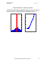
14.2 DESCRIPTION OF DATA DISTRIBUTION WITH DEPTH.................................................................. 55
14.3 PROBLEM.....................................................................................................................55
14.4 APPROACH FOR THE PROBLEM SOLUTION............................................................................55
Copyright © 2004 by Satlantic Incorporated
iv
ProSoft User Manual 7.7
SAT-DN-00228
14.5 EXAMPLES................................................................................................................... 56
....................................................................................................................................... 59
Copyright © 2004 by Satlantic Incorporated
v
ProSoft User Manual 7.7
SAT-DN-00228
List of Equations
EQUATION 1 GENERAL CALIBRATION EQUATION...................................................30
EQUATION 2 NULL DARK............................................................................................. 31
EQUATION 3 BIN DARK................................................................................................ 31
EQUATION 4 HYPERSPECTRAL DARK ...................................................................... 31
EQUATION 5 HYPERSPECTRAL DATA CALIBRATION............................................. 31
EQUATION 6 HYPERSPECTRAL DARK CORRECTION..............................................32
EQUATION 7 DARK DATA DEGLITCHING................................................................... 32
EQUATION 8 STANDARD DEVIATION......................................................................... 32
EQUATION 9 PRESSURE FILTERING.......................................................................... 35
EQUATION 10 DIFFUSE ATTENUATION COEFFICIENT (OCEAN OPTICS
PROTOCOLS FOR SEAWIFS EQN. 26 PG. 49)............................................................ 38
EQUATION 11 OCEAN OPTICS PROTOCOLS FOR SEAWIFS EQN. 31 PG. 50........38
EQUATION 12 AUSTIN PETZOLD 490NM.................................................................... 39
EQUATION 13 AUSTIN PETZOLD 520NM.................................................................... 40
EQUATION 14 MOREL 1988.......................................................................................... 40
EQUATION 15 MOREL 1988 EQUATION 9................................................................... 40
EQUATION 16 SURFACE VARIABLES (OCEAN OPTICS PROTOCOLS FOR
SEAWIFS EQN. 31 PG. 50)............................................................................................ 41
EQUATION 17 ES(0-)......................................................................................................41
EQUATION 18 LS(0-)...................................................................................................... 41
EQUATION 19 NORMALIZED WATER LEAVING RADIANCE (OCEAN OPTICS
PROTOCOLS EQN. 63 PG. 54)...................................................................................... 42
EQUATION 20 WATER LEAVING RADIANCE..............................................................42
EQUATION 21 ED(0+).....................................................................................................42
EQUATION 22 SURFACE REMOTE SENSING REFLECTANCE................................. 43
EQUATION 23 ABOVE SURFACE ED(0+).................................................................... 43
Copyright © 2004 by Satlantic Incorporated
vi
ProSoft User Manual 7.7
SAT-DN-00228
EQUATION 24 WATER LEAVING RADIANCE..............................................................43
EQUATION 25 REMOTE SENSING REFLECTANCE PROFILE................................... 43
EQUATION 26 SURFACE REFLECTANCE................................................................... 44
EQUATION 27 ABOVE SURFACE ED(0+).................................................................... 44
EQUATION 28 ABOVE SURFACE EU(0+).................................................................... 44
EQUATION 29 REFLECTANCE PROFILE.....................................................................45
EQUATION 30 PHOTOSYNTHETICALLY AVAILABLE RADIATION...........................45
EQUATION 31 PERCENTAGE PAR.............................................................................. 45
EQUATION 32 REFERENCE PAR................................................................................. 45
EQUATION 33 MOREL 98 CHLOROPHYLL MODEL....................................................46
EQUATION 34 CHLOROPHYLL A SURFACE ESTIMATE SEABAM OC2 MODEL.... 46
EQUATION 35 CALCULATION OF R COEFFICIENT................................................... 46
EQUATION 36 CHLOROPHYLL A SURFACE ESTIMATE GORDON 88 MODEL....... 47
EQUATION 37 CHLOROPHYLL A SURFACE ESTIMATE GORDON 88 MODEL....... 47
EQUATION 38 ESTIMATION OF ENERGY FLUXES.................................................... 47
EQUATION 39 VOLUME SCATTERING OF PARTICLES.............................................48
EQUATION 40 VOLUME SCATTERING OF WATER.................................................... 48
EQUATION 41 PARTICULATE BACKSCATTERING COEFFICIENT...........................48
EQUATION 42 BACKSCATTERING COEFFICIENT PURE WATER............................ 48
EQUATION 43 BACKSCATTERING COEFFICIENT SEA WATER...............................48
EQUATION 44 TOTAL BACKSCATTERING COEFFICIENT........................................ 48
Copyright © 2004 by Satlantic Incorporated
vii
ProSoft User Manual 7.7
SAT-DN-00228
1. Introduction
ProSoft is a data analysis package for processing data collected from oceanographic
measurement systems. The primary goal of the program was to create a package that
would be able to process optical data in an automated manner so that processing of
data was not subjective and any two investigators would get the same results from the
same data set. With the increasing number of different instrument types that can be
used from the autonomous buoys, from ships, or from airborne platforms, a demand for
a generalized approach for processing all optical data has emerged. To meet this
demand, ProSoft has been created. The most important changes have been related to
data and metadata organization, which is now based on the Hierarchical Data Format
(HDF 4), developed by The National Center for Supercomputing Applications at
University of Illinois at Urbana-Champaign http://hdf.ncsa.uiuc.edu/. At the same time,
the principles of data processing have not changed. Any principle changes that will be
introduced in the future will be stated explicitly (they can be found in the program under
menu ‘Help->About’). ProSoft allows users to read, calibrate, average and inspect data
sets collected from their instrumentation.
The program is currently supported by Satlantic
ftp://ftp.satlantic.com/pub/sensors/software/ProSoft/
Inc.
Copyright © 2004 by Satlantic Incorporated
and
is
available
at
1
ProSoft User Manual 7.7
SAT-DN-00228
2. System Requirements
ProSoft's source code is completely written in MatLab® version 6.5.1. Thus the system
requirements for ProSoft are defined by the system requirements of MatLab, which are
as follows:
OS: Microsoft® Windows® 95, Windows 98 (original and Second Edition), Windows
Millennium Edition, Windows NT 4.0, Windows 2000 or Windows XP.
Processor: Pentium®, Pentium Pro, Pentium II, Pentium III, Pentium IV or AMD® Athlon
based personal computer.
Current version of ProSoft has been compiled on PC with Pentium IV processor, under
Windows XP.
We suggest using a minimum of 256 MB of RAM.
Copyright © 2004 by Satlantic Incorporated
2
ProSoft User Manual 7.7
SAT-DN-00228
3. Installation
ProSoft is available as a standard Microsoft® Windows® 95/98/NT/XP install and is
supplied on CD or as a single self-extracting program from our Internet site at the above
ftp address. One should run the ProSoft#.#_Setup.exe program and follow the
instructions on the screen.
Copyright © 2004 by Satlantic Incorporated
3
ProSoft User Manual 7.7
SAT-DN-00228
4. Revisions
4.1 ProSoft 7.7
1. Changed graphics renderer mode to zbuffer which renders 3-D graphics in much
less time.
2. When graphing hdf file data, users are now able to select which independent
variables to graph as well as the range of the dependant variable.
3. New graphical overlay option allows users to graph data from different dependant
variables belonging to the same instrument group onto the same graph.
4. Any number of ECO Sensor IOP sensors can now be processed for an instrument.
Most calibration file definitions are acceptable for an ECO Sensor IOP.
5. Improved reliability of sensor distances from surface and pressure reference
distances.
6. Sample delay time correction has now been applied to timer values where
appropriate at level 2 processing.
7. Transmissometer sensor has been added to level 2s and 3a data processing.
8. Added Reference Ef Ev and Ld optical sensors to level 2s and 3a data processing.
9. Any kind of profiler can now be used in Reference mode. The mode is indicated in
the instrument context by selecting Reference as the instrument type.
10. Improved dynamic data processing at levels 2s and 3a.
11. All GPS telemetry definitions are now supported.
12. Added the ability to process upcasts and downcasts within the same telemetry file.
13. ECO Series IOP sensors with backscatter sensors can now process backscattering
coefficients as a Level 4 data product.
14. Added new tool that allows conversion of ProSoft generated hdf files into Matlab
binary files (*.mat) which can be imported directly into the Matlab workspace.
4.2 ProSoft 7.6
1. GPS sensor data integrated into profiler/reference configurations. GPRMC, GPGLL
and GPGGA only are supported.
2. TSRB mode added for all profiler/reference configurations including HyperPro II.
3. Level 4 water properties data product enabled. Instrument must have a profiler with
Temp and Cond sensors.
4. Level 2s depth integration resolution is now adjustable to 0.01, 0.02, 0.05 and 0.10m
through parameters settings.
5. Sas integration time interval is now derived on the interval of the optical sensor with
the highest rate instead of the standard of 0.1sec.
6. Conductivity sensor data included to level 3a.
7. Temperature sensor data included to level 3a.
Copyright © 2004 by Satlantic Incorporated
4
ProSoft User Manual 7.7
SAT-DN-00228
8. Fluorometer sensor data included to level 3a.
9. File batch processing sequence changed. Instead of processing all files together at
one level (i.e. process all files at level 1a before processing all files at level 1b), each
file is processed separately from level 1a to selected level.
10. Calibration files can now be added or removed from configuration files that are
created from *.sip files.
11. Imported configuration files can now be saved with their original file name by clicking
on 'Save' in the configuration utility.
12. Reference only or TSRB mode data are now integrated onto the time interval derived
from the Es sensor instead of the previous standard of 0.1 sec.
13. Added Reference Ev optical sensor to processing at all levels.
4.3 ProSoft 7.5
1. Added support for level 2s GPS integration for the following GPS formats $GPRMC,
$GPGLL and $GPGGA.
2. SAS GPS data is now averaged at level 3a.
3. GPS data is not available for viewing below level 2s in the hdf viewer but can be
extracted using the ascii data extractor.
4. Added support for the ECO Series IOP sensor for the new HyperPro II instrument.
5. Faster ascii data extraction of hdf files.
6. Fixed bugs preventing processing of TSRB data.
4.4 ProSoft 7.4
1. Processing parameters have been incorporated into one file. Access to the file is
through the new processing parameters utility.
2. Processing parameters can be easily edited through the new parameters interface.
All four levels of parameters are viewed and edited at once.
3. Processing parameters have been separated from the instrument context. The new
‘Processing Context’ consists of both the current instrument and current processing
parameters.
4. HDF viewer now includes the ability to save the graph image as a file using the png
graphic format.
5. Updated ProSoft main menu. Processing level commands have been moved to the
main menu for easier use. Ascii data extractor and HDF viewer are now accessible
through the menu selection ‘Tools’.
6. Instrument context creation/edit utility now allows adding or removing calibration files
from the instrument context.
4.5 ProSoft 7.3
1. New level 2s file is introduced for all instruments. The Level 2s file shows the
interpolated data just prior to averaging at Level 3a.
Copyright © 2004 by Satlantic Incorporated
5
ProSoft User Manual 7.7
SAT-DN-00228
2. Introduction of ‘Instrument Context’ creation and loading for easy data processing
and selection between different instruments.
3. Added processing support for Satlantic Satnet instruments.
4. Easier to use Ascii data extraction utility.
5. Updated ProSoft main menu interface.
6. Addition of completely revised HDF graphical viewer utility which makes it possible to
graph all HDF files in 2-D or 3-D graphical views.
7. Updated and easier to use configuration file creation/edit utility.
8. Level 4 chlorophyll a profile estimates using Morel 98 model added.
9. Level 4 chlorophyll a surface estimates using SeaBAM OC2 model (Rrs) added.
10. Level 4 chlorophyll a surface estimates using Gordon 88 model (Lwn) added.
11. Level 4 energy profile/surface fluxes added.
12. Sas data can now be processed to level 3a.
Copyright © 2004 by Satlantic Incorporated
6
ProSoft User Manual 7.7
SAT-DN-00228
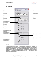
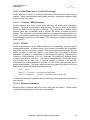
5. Overview
Edit current
instrument context
Delete current instrument
context
Create new
instrument context
Import existing
instrument context
Edit current
parameters
Delete parameters
context
Create new
parameters
Process data from
raw to level 2
Process data from raw
to level 2s
Process data from raw
to level 3a
Process data from raw
to level 4
Process data from raw
to level 1a
Process data from
level 1a to level 1b
Process data from level
1b to level 2s
Process data from level
2s to level 3a
Process data from
level 3a to level 4
5.1 Processing Context
The processing context defines all the parameters necessary for processing of
instrument data. The processing context is made up of two parts, the current instrument
and the current parameters. The current instrument defines the instrument used for
gathering the raw data. See instrument context for details. The current parameters
defines all the processing variables for level 1 to level 4 data processing. See
parameters context for details.
Copyright © 2004 by Satlantic Incorporated
7
ProSoft User Manual 7.7
SAT-DN-00228
5.1.1 Current Instrument
Displays the currently loaded instrument context. All instrument configuration information
is loaded and ready for processing. See instrument context for details.
5.1.1.1 New
Starts the process for creating a new instrument context. The user is asked to supply the
location of the calibration file(s) or sip file(s) for the instrument, which are then used to
create the instrument context. Note: All calibration file(s) (*.cal) or sip file(s) (*.sip)
for the instrument context must remain in the same directory as the instrument
context (*.cfs) file.
5.1.1.2 Import
Allows the user to import an existing instrument context file (*.cfs) for use in a new
instrument context.
5.1.1.3 Edit
This option loads the current instrument context into the instrument context utility for
editing. The user can choose to save the file under the existing instrument context name
(‘Save’) or create a new instrument context (‘Save As’).
5.1.1.4 Delete
Permanently deletes the current instrument context. The context file (*.cfs) associated
with the instrument context is not deleted.
5.1.2 Current Parameters
Displays the currently loaded parameters context. All processing parameters are loaded
and ready for processing. See parameters context for details.
5.1.2.1 New
Starts the process for creating a new processing parameters context. The processing
parameters utility will display with default values automatically loaded.
5.1.2.2 Edit
This option loads the current processing parameters into the processing parameters
utility for editing. The user can choose to save the file under the existing processing
parameters context name (‘Save’) or create a new parameters context (‘Save As’).
5.1.2.3 Delete
Permanently deletes the loaded processing parameters context. The original parameters
file (*.mat) associated with the processing parameters context is also deleted.
Copyright © 2004 by Satlantic Incorporated
8
ProSoft User Manual 7.7
SAT-DN-00228
5.2 Multi-Level Processing
Multi-level processing enables the user to process raw data up to level 2s, level 3a or
level 4. All intermediate processing levels are automatically processed with
accompanying files (*.hdf) being produced. To use this feature select the command
button according to the ending processing level as desired. ProSoft will prompt the user
to select the directory and choose file(s) (*.raw) of raw data.
5.3 Single Level Processing
Single level processing enables the user to process data over a single level. For
example from level 1a to level 1b. To use this feature select the command button
according to the starting processing level and ending processing level as desired.
ProSoft will prompt the user to select the directory and choose file(s) (*.hdf or *.raw) for
the starting processing level.
5.4 Tools Menu
5.4.1 Ascii Data Extractor
This utility converts hdf files to tab separated ascii file format. ProSoft will prompt the
user to select the directory and choose file(s) (*.hdf) for ascii data extraction. Hdf files at
any level except raw (*.raw) can be extracted. See ascii data extraction for details.
5.4.2 MAT Data Extractor
This utility converts hdf files into a Matlab data structure. This structure is then saved
into Matlab binary format (*.mat) which can be directly imported into the Matlab
workspace for further analysis and manipulation. See mat data extraction for details.
5.4.3 HDF Viewer
Select this option to access the HDF viewer utility which allows the user to view hdf files
in 2-D or 3-D graphical format. The utility will open in the empty state. Simply select ‘File
-> Open’ to load hdf files for viewing. See hdf data viewer for details.
5.5 Help Menu
5.5.1 Definitions
Select this option to view a list of definitions of ProSoft terms. See appendix A term
definitions for list of definitions.
5.5.2 About
Select this option to view the history of revisions for ProSoft versions. This lists the latest
changes made to ProSoft. See revisions for details.
Copyright © 2004 by Satlantic Incorporated
9
ProSoft User Manual 7.7
SAT-DN-00228
5.6 File Menu
5.6.1 Exit
Select this option to exit the current ProSoft session. The last loaded instrument context
and processing parameters context will be automatically loaded next time ProSoft is
started.
Copyright © 2004 by Satlantic Incorporated
10
ProSoft User Manual 7.7
SAT-DN-00228
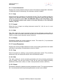
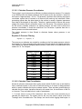
6. Instrument Context
Instrument Context Utility
Instrument Context is defined as the current instrument package (i.e. profiler +
reference) loaded into ProSoft that will be used for data processing. The instrument
context file (*.cfs) used to describe this instrument is loaded into memory ready to be
recalled when necessary for processing.
The user can switch between instrument packages easily by clicking on the drop down
box and selecting from the list of instrument contexts that have been defined by the user.
When an instrument is chosen the instrument context file associated with the instrument
package is automatically loaded and ProSoft is ready to process data.
6.1 Available Calibration Files
This is a list of all calibration files (*.cal and .tdf) located in the current directory or files
associated with a sip file (*.sip). In the case of creating a new instrument context the
current directory or sip file(s) are selected prior to displaying the instrument context
utility. When editing or importing, the current directory is the directory that the instrument
context file is located in.
6.2 Loaded Calibration Files
This is a list of all calibration files (*.cal and *.tdf) that are loaded in the instrument
context. These are the calibration files which will be associated with the instrument
context. These can be added or removed as needed.
Copyright © 2004 by Satlantic Incorporated
11
ProSoft User Manual 7.7
SAT-DN-00228
6.3 Calibration File Parameters
The ‘Calibration File Parameters’ displays all current configuration information on the
calibration file selected in the ‘Loaded Calibration Files’ selection box. See table
‘Calibration File Settings’.
6.3.1 Sensors
This is a list of optical sensors defined within the selected calibration file.
6.3.2 Frame Tag
Indicates the frame tag associated with the calibration file as it appears in the raw or
level 1 telemetry data.
6.3.3 Instrument Type
Select the type of instrument represented by the calibration file. For a list of possible
values see instrument context parameters and calibration file settings tables.
6.3.4 Immersion Coefficient
Select which calibration coefficients to use for processing depending on instrument
immersion mode (i.e. Air or Water).
6.3.5 Measurement Mode
Select which mode of measurement to use for processing the calibration file and it’s
associated raw data.
6.3.6 Frame Type
Select the frame type for the calibration file for dark current correction calculations.
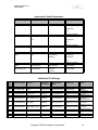
6.3.7 Instrument Context Parameters
The instrument context parameters table indicates all the possible combinations of
selectable configuration parameters based on the instrument type.
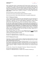
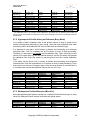
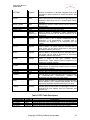
6.3.8 Calibration File Settings
The calibration files settings table indicates the instrument parameters settings based on
calibration file prefix. The prefix is obtained from the first three letters of the calibration
file name which is listed in ‘Loaded Calibration Files’ in the instrument context utility.
Copyright © 2004 by Satlantic Incorporated
12
ProSoft User Manual 7.7
SAT-DN-00228
Instrument Context Parameters
Instrument Type
Immersion Coefficient
Measurement Mode
Frame Type
Profiler
Water
FreeFall
ShutterLight
ShutterDark
Anc
LightAncCombined
Reference
Water
Surface
Air
ShutterLight
ShutterDark
Anc
LightAncCombined
TACCS
Water
Chain
LightAncCombined
SAS
Air
VesselBorne
ShutterLight
AirBorne
ShutterDark
Anc
LightAncCombined
GPS
Not Required
Not Required
Not Required
ECO Series IOP
Not Required
FreeFall
Not Required
Surface
Calibration File Settings
Cal
File
Prefix
Instrument Type
Sensors
Immersion
Coefficients
Measurement
Mode
Frame Type
Notes
BB2F
ECO Series IOP
Fluor
Not Required
[FreeFall Surface]
Not Required
Wetlabs
Fluorometer
DI4
Profiler/Reference
[Lu Ld]**/Ls
Water/Air
FreeFall/Surface
LightAncCombined
4 channel
irradiance sensor
DR4
Profiler/Reference
[Ed Eu]/[Es Ev Ef]
Water/Air
FreeFall/Surface
LightAncCombined
4 channel
radiance sensor
DI7
Profiler/Reference
[Lu Ld]/Ls
Water/Air
FreeFall/Surface
LightAncCombined
7 channel
irradiance sensor
DR7
Profiler/Reference
[Ed Eu]/[Es Ev Ef]
Water/Air
FreeFall/Surface
LightAncCombined
7 channel
radiance sensor
HED
Reference/Sas
Es/Es
Air/Air
Surface/VesselBor
ne
ShutterDark
Hyperspectral
HLD
Reference/Sas
Ls/Lt
Water/Air
Surface/VesselBor
ShutterDark
Hyperspectral
Copyright © 2004 by Satlantic Incorporated
13
ProSoft User Manual 7.7
SAT-DN-00228
ne
HSE
Reference/Sas
Es/Es
Air/Air
Surface/VesselBor
ne
ShutterLight
Hyperspectral
HSL
Reference/Sas
Ls/[Lt Li]
Water/Air
Surface/VesselBor
ne
ShutterLight
Hyperspectral
HPE
Profiler
Ed
Water
FreeFall
ShutterLight
Hyperspectral
HPL
Profiler
Lu
Water
FreeFall
ShutterLight
Hyperspectral
HSD
Reference
Lu
Water
Surface
ShutterDark
Hyperspectral
TSRB
HST
Reference
Lu
Water
Surface
ShutterLight
Hyperspectral
TSRB
MPR*
Profiler/Ancillary
Lu Ed Eu Ld/Tilt
Press T
Water/[Water
Air]
FreeFall/[FreeFall
Surface]
LightAncCombined/
Anc
Multispectral/
Ancillary
MRF
Sas
Ls Lt Es
Air
VesselBorne
LightAncCombined
Multispectral
MVD
Reference
Es Ls Ef Ev
Air
Surface
LightAncCombined
Multispectral
OCP
Profiler
Lu Ed Eu Ld
Water
FreeFall
LightAncCombined
Multispectral
PED
Profiler
Ed
Water
FreeFall
ShutterDark
Hyperspectral
PLD
Profiler
Lu
Water
FreeFall
ShutterDark
Hyperspectral
PRO
Profiler
Lu Ed Eu Ld
Water
FreeFall
LightAncCombined
Multispectral
REF
Reference
Es Ls Ef Ev
Air
Surface
LightAncCombined
Multispectral
TAC
Taccs
Lu Ed Es
Water
Chain
LightAncCombined
Multispectral
* MPR calibration files can be either a profiler or ancillary instrument. It’s most common
use is as an ancillary instrument which can be determined by it’s lack of optical sensors
(i.e. Lu Ed). When used as an ancillary instrument it’s measurement mode can be either
FreeFall if attached with a profiler or Surface if attached with a reference. The frame type
when used as ancillary should be Anc.
** [ ] Brackets indicate mutually exclusive sensors. For example [Lu Ed] indicates only Lu
or Ed sensor will be present but never both.
6.4 Sensor Parameters
The ‘sensor parameters’ displays all current configuration information on the sensor
selected in the ‘Sensors’ selection box.
6.4.1 Channels
All the channels available from the selected optical sensor are displayed here. For
optical sensors this will be a list of all sensor wavelengths.
6.4.2 Configuring Sensor Distances
The sensor head distances are needed in order to compensate for the fact that the
pressure sensor is not located at the same position as the sensor heads. In order to
calculate the pressure at the sensor head this geometrical difference must be known and
included in the instrument context file (all units must be in meters).
Copyright © 2004 by Satlantic Incorporated
14
ProSoft User Manual 7.7
SAT-DN-00228
When configuring a profiler it is assumed that the Ed sensor head is located at the ‘top’
of the instrument. In other words it is the last sensor to be immersed when profiling. For
the profiler it is important to include the distance between each sensor head and the Ed
sensor head (top of the instrument). This value is entered into ‘Distance to Surface’. The
‘Distance to Pressure’ value is only required for the Ed sensor when taking the pressure
tare on deck as outlined below in ‘Distance to Pressure’. In all other cases leave this
value at zero.
Sas instruments do not need to specify any distances.
ECO Series IOP sensors should always specify the distance to surface.
When the pressure tare is taken during measurements, two possible methods exist.
6.4.2.1 Distance to Surface
This is the physical distance between the sensor head and the top of the instrument for
profilers, and the distance between the sensor head and the surface of the water, if
immersed, for references. This value should always be specified for sensors located
below the top of the instrument (i.e. Lu sensor, ECO Series IOP sensor, Ls sensor).
Pressure tare is taken when the Ed sensor is located at the surface of the water. In
this, the most common method, the pressure tare then becomes a combination of the
atmospheric pressure and the pressure of the water column from the surface (Ed head)
to the pressure sensor reference line. The pressure value at Ed is calculated by
subtracting the pressure tare value from the measured pressure values. The pressure
value at Lu is calculated by subtracting the pressure tare value from the measured
pressure values, as calculated for Ed, and then adding the distance between the Lu
sensor head and the Ed sensor head.
When using this pressure tare mode it is very important that you do not include any
values in ‘Distance to Pressure’ for any sensors. These should be set to zero and is
reserved for the situation outlined in 2 below.
Pressure Ed = Measured Pressure – Pressure Tare
Pressure Lu = Measured Pressure – Pressure Tare + Distance to Surface (Lu)
6.4.2.2 Distance to Pressure
This value is used only for profiler sensors to indicate the distance between the sensor
head and the pressure reference line on the profiler and should only be given values
when obtaining pressure tare on deck.
Pressure tare is taken when the profiler is located on deck. In this case the pressure
tare is equal to the atmospheric pressure. The pressure tare value is then added to the
distance from the Ed head to the pressure sensor reference line. For this reason it is
crucial to specify a ‘Distance to Pressure’ for the Ed sensor in the instrument context
utility.
Pressure Tare = Pressure Tare (Atmospheric Pressure) + Distance to Pressure (Ed)
Pressure Ed = Measured Pressure – Pressure Tare
Pressure Lu = Measured Pressure – Pressure Tare + Distance to Surface (Lu)
Copyright © 2004 by Satlantic Incorporated
15
ProSoft User Manual 7.7
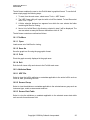
SAT-DN-00228
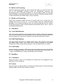
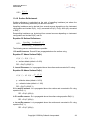
Note: Instrument configurations and distances may not be the same for your
instrument. Always measure distances when creating an instrument context file
for your instrument. The diagrams below indicate the most common
configurations available.
Sea Level
Ed Sensor
Lu Sensor
Atmospheric
Pressure
Lu Distance to
Ed Head
Pressure
Tare
Ed Distance
to pressure
reference
Pressure reference
line
Lu Distance
Reference: Ed Head
0.101346 m
Ed Distance
Reference: Pressure
0.663575 m
Pressure
Reference Line
Profiler Sensor Dimensions
Copyright © 2004 by Satlantic Incorporated
16
ProSoft User Manual 7.7
SAT-DN-00228
6.5 Creating a New Instrument Context
When using ProSoft for the first time a warning message is given stating that no
instrument context has been defined. To create a new instrument context use the
following steps:
1. Click on ‘New’ in the ProSoft main menu.
2. ProSoft will ask the user to point to a directory containing all the calibration files
(*.cal) or sip files (*.sip). Note: The calibration files and instrument context
file *.cfs should always remain together in the same directory.
3. The instrument context utility will then display showing a list of all available
calibration (*.cal) and tdf files (*.tdf) located in the directory selected in step 2.
4. Highlight all the calibration files in ‘Available Calibration Files’ needed for the
instrument context and click on add ‘>>’ to load the calibration files. For sip files
this step is not necessary as the calibration files are automatically loaded.
5. Configure all calibration file and sensor parameters as necessary and click on
‘Save As’.
6. The user is then prompted to enter an instrument context name. Once entered
click on ‘Ok’.
7. A dialogue box will then display confirming that the instrument context has been
successfully created. Click on ‘Ok’ and ProSoft will load the instrument context
just created.
Whenever the user exits the program, ProSoft remembers the last instrument context
that was loaded and automatically reloads that context when starting ProSoft.
6.6 Configuring GPS
To include GPS data in processing, several *.tdf and *.sip files have been included in the
ProSoft installation directory. Simply copy these files into the same directory as the *cal
or *.sip files being used for the instrument processing. When the instrument calibration
files are bundled into *.sip files then use the gps.sip file exclusively, or if using *.cal files
for the instrument then use any of the *.tdf GPS files. More than one type of GPS *.tdf
file may be included in the ‘Loaded Calibration Files’ column. Sensor dimensions are not
required for GPS.
6.7 Instrument Context Examples
6.7.1 Hyperspectral Profiler/Reference (HyperPro)
The hyperspectral profiler/reference configuration is very common and usually contains
a large number of calibration files (*.cal) and some tdf files (*.tdf). When working with
hyperspectral instruments each optical sensor has two calibration files, one for
shutterlight and the other for shutterdark frames.
Calibration File
Instrument Type
Immersion
Coefficient
Measurement
Mode
Frame Type
Hed117g.cal
Reference (Es)
Air
Surface
ShutterDark
Copyright © 2004 by Satlantic Incorporated
17
ProSoft User Manual 7.7
SAT-DN-00228
Hpe116h.cal
Profiler (Ed)
Water
FreeFall
ShutterLight
Hpl118h.cal
Profiler (Lu)
Water
FreeFall
ShutterLight
Hse117g.cal
Reference (Es)
Air
Surface
ShutterLight
Mpr012b.cal*
Profiler (Anc)
Water
FreeFall
Anc
Ped116h.cal
Profiler (Ed)
Water
FreeFall
ShutterDark
Pld118h.cal
Profiler (Lu)
Water
FreeFall
ShutterDark
Bb2f-054.tdf
ECO Series IOP
Not Required
FreeFall
Not Required
Gprmc.tdf
Gps
Not Required
Not Required
Not Required
* The Mpr012b.cal file is an ancillary sensor attached to the profiler and is therefore given Profiler as
instrument type and FreeFall as measurement mode. The FrameType is set as Anc to distinguish it from an
optical sensor.
6.7.2 Hyperspectral Profiler Acting as Reference (Buoy Mode)
It is possible to add a floatation collar to the profiler sensors to have it remain at the
surface collecting data and acting in buoy mode. Using the same calibration files when
used as a profiler, each calibration file is set to Reference as instrument type.
It is important to note that if an Ed sensor is present and functioning as a reference
instrument then it will be re-labeled as an Es sensor at level 2s data processing.
Therefore it is important to not include the Ed calibration files. There must only be one
source of Es sensor data, so the user should choose to use the Es sensor and exclude
the calibration files for the Ed sensor by removing them from the ‘Loaded Calibration
Files’.
In the same way as above if an Lu sensor is present and functioning as a reference
instrument then it will be re-labeled as an Ls sensor at level 2s data processing. There
must only be one source of Ls sensor data, so the user must choose to use either the Lu
or Ls sensor and exclude the calibration files for the one not in use.
Calibration File
Instrument Type
Immersion
Coefficient
Measurement
Mode
Frame Type
Hse117g.cal
Reference (Es)
Air
Surface
ShutterLight
Hpl118h.cal
Reference (Lu)
Water
Surface
ShutterLight
Mpr012b.cal
Reference (Anc)
Air
Surface
Anc
Hed117g.cal
Reference (Es)
Air
Surface
ShutterDark
Pld118h.cal
Reference (Lu)
Water
Surface
ShutterDark
6.7.3 Multispectral Profiler/Reference (MicroPro)
Non-hyperspectral optical sensors usually use a LightAncCombined frame type. In many
cases one calibration file will contain more than one optical sensor.
Calibration File
Instrument Type
Immersion
Coefficient
Measurement
Mode
Frame Type
DI7106a.cal
Reference (Es)
Air
Surface
LightAncCombined
Copyright © 2004 by Satlantic Incorporated
18
ProSoft User Manual 7.7
SAT-DN-00228
DI7112a.cal
Profiler (Ed)
Water
FreeFall
LightAncCombined
DI7113a.cal
Profiler (Ed)
Water
FreeFall
LightAncCombined
DR7112a.cal
Profiler (Lu)
Water
FreeFall
LightAncCombined
DR7113a.cal
Profiler (Lu)
Water
FreeFall
LightAncCombined
Mpr049a.cal
Profiler (Anc)
Water
FreeFall
Anc
Copyright © 2004 by Satlantic Incorporated
19
ProSoft User Manual 7.7
SAT-DN-00228
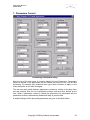
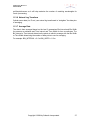
7. Parameters Context
Processing Parameters Utility
Near the top of the main menu is a section labeled ‘Current Parameters’. Parameters
context is defined as the parameters that are loaded into memory to be used for data
processing. For example they determine what type of dark correction to apply or how
many data points to use when averaging.
The user can easily switch between parameters contexts by clicking on the drop down
box and selecting from the list of parameters contexts that have been defined by the
user. When a parameters context is chosen the parameters file associated with the
parameters context is automatically loaded and ready to process data.
A detailed listing of all the processing parameters are given in the tables below.
Copyright © 2004 by Satlantic Incorporated
20
ProSoft User Manual 7.7
SAT-DN-00228
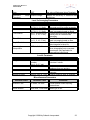
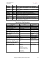
Dark Correction Parameters
Parameter Name
Parameter Values
Auto Dark Correction
Comments
CAL
Darks from cal file
BIN
Darks from profile
SHUTTER
Darks from shutter frames
Dark Bins
Positive Integer
Number of data points that are used to
obtain bin darks from profile. Thus Dark
Bins is used only if Auto Dark Correction
is set to BIN.
Shutter Dark Deglitch
ON
ON – First difference filter will be
supplied to deglitch shutter dark frames
of optical data.
OFF
Tilt Editing Parameters
Parameter Name
Parameter Values
Auto Edit
ON
OFF
Comments
Automated profiler data editing using tilts
or falling velocity when Tilt Edit is ON.
ON – automatic editing
OFF – interactive editing
Tilt Edit
ON
Toggles tilt edit mode on or off.
OFF
Low Velocity
Positive integer
If tilt edit and auto edit are turned ON,
low velocity will be used for automatic
editing only if tilt sensor is missing.
High Tilt
Positive integer
If tilt edit and auto edit are turned ON,
high tilt will be used for automatic tilt
editing.
Data Filtering Parameters
Parameter Name
Parameter Values
Deglitch Profiler Data
ON
OFF
Profiler
Threshold
Noise Positive Integer
Comments
If ON, profiler data is deglitched using the
value of Profiler Noise Threshold.
Adjusts the sensitivity of profiler data
deglitching.
Upper Depth Level
Positive Integer
Sets shallow depth level below which
profiler data is deglitched.
Lower Depth Level
Positive Integer
Sets deep depth value above which
profiler data is deglitched.
Deglitch
Reference ON
If ON, reference data is deglitched using
Copyright © 2004 by Satlantic Incorporated
21
ProSoft User Manual 7.7
SAT-DN-00228
Data
Reference
Threshold
OFF
the value of Reference Noise Threshold.
Noise Positive Integer
Adjusts the sensitivity of reference data
deglitching.
Level 3a Averaging Parameters
Parameter Name
Bin Interval
Bin Width
Time Interval
Time Width
Depth Resolution
Wavelength
Interpolation
Parameter Value
Any 0.1m interval (i.e.
0.2, 0.6, 1.2, 2.0 etc)
Any 0.1m interval (i.e.
0.2, 0.6, 1.2, 2.0 etc)
Any 1 second interval
(i.e. 1, 2, 10, 17 etc.)
Any 1 second interval
(i.e. 1, 2, 10, 17 etc.)
Variable
OFF, 1, 2, 5, 10
Comments
Controls the depth interval which is
the center point for profiler averaging.
Controls the number of data points
used in averaging based on depth.
Controls the time interval which is the
center point for reference/Sas
averaging.
Controls the number of data points
used in averaging based on time.
Controls the depth resolution used for
data integration at level 2s.
Controls the interpolation interval
when interpolating onto a constant
wavelength. Only applicable for
hyperspectral instruments.
Level 4 Constants
Parameter Name
Integration Points
Reflection Albedo
Parameter Value
Must be an odd
number
(i.e. 1, 3, 5, 7 etc.)
Default value of 0.043
Reflectance Index
Default value of 0.021
Refractive Index
Default value of 1.345
Comments
Number of data points used to
calculate K values.
Fresnel reflection albedo for
irradiance from sun and sky.
Fresnel reflectance index of
seawater.
Fresnel refractive index of seawater.
Miscellaneous Parameters
Parameter Name
Parameter Value
Comments
Pressure Tare
In Water, On Deck
Profiler position when acquiring
pressure tare.
Water Medium
Sea water, Fresh water
Water type in-situ.
Copyright © 2004 by Satlantic Incorporated
22
ProSoft User Manual 7.7
SAT-DN-00228
8. ASCII Data Extraction
The ascii data extractor utility allows the user to convert any ProSoft hdf file into tab
separated ascii file format. This format can be used to import data into an excel
spreadsheet or other program that can use ascii tab delimited files.
To extract hdf files use the following procedure:
1. From the main menu click on menu ‘Tools -> Ascii Data Extractor’.
2. A folder selection dialogue will appear from which the user selects a folder with
the hdf files to be extracted.
3. Next a list of all hdf files in the directory selected in step 2 will be displayed. The
user can select as many hdf files as desired.
4. Click on ‘Ok’ to start the file extraction process.
All the extracted ascii files will be place in a directory called ‘Ascii Files’. This directory
will be located in the same directory as the hdf files selected in step 2. If the ‘Ascii Files’
directory cannot be created then the ascii files will be located in the same directory as
the hdf files selected in steps 2 and 3.
ProSoft will write up to a maximum of 256 columns per row after which the data will wrap
to the next section of rows. This ensures the ascii file can be imported to excel without
loss of data.
Included in the ascii file is the hdf file header which includes metadata important for data
interpretation.
Copyright © 2004 by Satlantic Incorporated
23
ProSoft User Manual 7.7
SAT-DN-00228
9. MAT Data Extraction
The mat data extractor utility allows the user to convert any ProSoft hdf file into a Matlab
structure which is saved into a Matlab binary file (*.mat). This format can be used to
import the hdf data structure directly into a Matlab workspace for further analysis and
manipulation.
To extract hdf files use the following procedure:
1. From the main menu click on menu ‘Tools -> MAT Data Extractor’.
2. A folder selection dialogue will appear from which the user selects a folder with
the hdf files to be extracted.
3. Next a list of all hdf files in the directory selected in step 2 will be displayed. The
user can select as many hdf files as desired.
4. Click on ‘Ok’ to start the file extraction process.
All the extracted MAT files will be placed in the same directory as the hdf files and have
the same file name as it’s corresponding hdf file but with the .mat file extension.
To import the hdf data structure into the Matlab workspace use the ‘load’ command or
simply double click on the *.mat file when viewed in the ‘Current Directory’. The structure
called ‘hdfdata’ will load into the Matlab workspace and is now available for analysis.
The field names in the hdfdata structure are representative of the vdata table names in
the hdf file.
Copyright © 2004 by Satlantic Incorporated
24
ProSoft User Manual 7.7
SAT-DN-00228
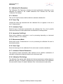
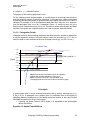
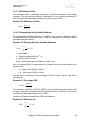
10. HDF Data Viewer
File menu: Access to printing graph,
loading new hdf files or quitting
Attributes menu: Access to hdf file
attributes, sensor group attributes
or sensor data table attributes
Hdf file selected for viewing
Select sensor group for viewing
Graph legend showing sensor fields
Graph title showing file name, cruise
identifier and processing level
Select range of independent variable
Select range of dependant variable
Select independent variable
Click to graph sensor fields
Graphing options All Fields, Grid, Rotate, Zoom
Select dependant variable
Select graph type, 2-D or 3-D
HDF Viewer
Copyright © 2004 by Satlantic Incorporated
25
ProSoft User Manual 7.7
SAT-DN-00228
The hdf viewer enables the user to view ProSoft data in graphical format. To use the hdf
viewer simply apply the following steps:
1. To start, from the main menu, select menu ‘Tools -> HDF Viewer’.
2. The HDF Viewer utility will open but with no hdf files loaded. To load files select
menu ‘File -> Open’.
3. A folder selection dialogue box appears from which the user selects the folder
containing hdf files for viewing.
4. Next a list of all hdf files in the directory selected in step 2 will be displayed. The
user can select as many hdf files as desired then click on ‘Ok’.
The hdf viewer controls are outlined as follows:
10.1 File Menu
10.1.1 Open
Loads a new set of hdf files for viewing.
10.1.2 Save As
Save the graph to a file using the png graphic format.
10.1.3 Print
Prints the graph currently displayed in the graph axes.
10.1.4 Exit
Exits the hdf viewer utility and returns to the ProSoft main menu.
10.2 Attributes Menu
10.2.1 HDF File
Select to view the hdf file attributes or metadata applicable to the entire hdf file such as
cruise id, date, processing level etc.
10.2.2 Sensor Group
Select to view the attributes or metadata applicable to the selected sensor group such as
instrument type, media, measurement mode etc.
10.2.3 Sensor Data Table
Select to view the attributes or metadata applicable to the selected sensor data table
such as units for each sensor field.
Copyright © 2004 by Satlantic Incorporated
26
ProSoft User Manual 7.7
SAT-DN-00228
10.3 HDF File Selected
This drop down box displays the current hdf file being viewed. All hdf files that were
selected for viewing are listed in this drop down box. To switch files simply click on the
drop down box and choose an hdf file.
10.4 Sensor Group
This control lists all the sensor groupings for the selected hdf file. Each sensor group
corresponds to an instrument calibration file. Common sensor groups are Profiler,
Reference, Sas, ECO Series IOP etc.
10.5 Independent/Dependant Variables
These controls list all the independent and dependent variables available for the chosen
sensor group.
10.6 Graph Type
Use the graph type buttons to select which type of graph is required. Note: Certain
sensor data tables are not available for viewing in 3-D. In this case the option for
selecting 3-D will be grayed out and unavailable for selection.
10.7 Graphing Options
10.7.1 Overlay
When this option is selected any subsequent graphing will overlay each other. This
useful for comparing data from different dependant variables.
10.7.2 Grid
When this option is selected a grid overlay will be drawn on the graph. This option is only
available for 2-D graphs as it is always on by default for 3-D graphs.
10.7.3 Rotate
When this option is selected the user is able to hold down the left mouse button while
over the graph and move the mouse to rotate the graph view. This option is only
available for 3-D graphs.
10.7.4 Zoom
When this option is selected the user is able to zoom in or out of the graph. To zoom in
left click the mouse button while over the graph and to zoom out right click the mouse
button. To select a portion of the graph to zoom, left click and hold the mouse button
while over the graph and drag the area selection box. When completed release the
mouse button and the graph will zoom on the area selected. This option is only available
for 2-D graphs.
Copyright © 2004 by Satlantic Incorporated
27
ProSoft User Manual 7.7
SAT-DN-00228
10.7.5 Graph
When all the desired independent/dependant ranges are selected click on ‘Graph’ to
draw the graph in the axes. When zooming or rotating a graph simply click on ‘Graph’ to
return the graph to it’s original view.
10.7.6 Legend
In 2-D graphing mode a legend is displayed on the axes showing the field color-coding
scheme for the graph. The legend can be moved by left clicking and dragging the legend
to a different location on the axes. Make sure the zoom option is turned off when moving
the legend. In 3-D graphing mode a color contour legend is displayed outside the axes,
relating color with z-axis value for easier viewing.
Copyright © 2004 by Satlantic Incorporated
28
ProSoft User Manual 7.7
SAT-DN-00228
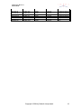
11. Data Processing Equations
Processing Levels Supported
Profiler
Reference
SAS
TSRB
TACCS
1a
X
X
X
X
X
1b
X
X
X
X
X
2
X
X
X
X
X
2s
X
X
X
X
3a
X
X
X
X
4
X
X
X
Note: Includes both multispectral and hyperspectral instruments
This section is intended to give an overview of the main steps of radiometric data L(z, λ)
processing carried out by ProSoft. It is assumed that the radiometric data has been
collected using an optical instrument with a raw data format that is in compliance with
Satlantic Instrument Files Standard (SIFS).
ProSoft processing is segmented into 4 main levels:
Level 1 - Raw binary data file from an instrument. File nametag is raw.
Level 1a - Binary data is extracted from raw data under the control of the instrument
(calibration and/or telemetry definition) files. Extracted information is grouped along with
its calibration information and is placed into Level 1a hdf files. File nametag is _L1a.
Level 1b - Level1b data is calibrated. No data editing is applied. Shutter darks, if
present, are not applied. File nametag is _L1b.
Level 2 - Includes Level 1b data, which is further modified per request (i.e. depending on
settings of processing parameters and on instrument context). File nametag is _L2.
1. Shutter dark correction is applied; reference and dark data deglitching is applied.
2. Profiler's data is tilt edited.
Level 2s – Level 2 data is interpolated onto a common co-ordinates vector, which is
either depth (Profiler) or time (Reference only or Sas). File nametag is _L2s.
Level 3a – Includes averaging of Level 2s data as defined by the processing
parameters. File nametag is _L3a.
Level 4 – Includes higher level data products (users choice) calculated from level 3a
data. This includes products such as normalized water leaving radiances, reflectance
profiles, photosynthetically available radiation etc. File nametag is _L4.
Copyright © 2004 by Satlantic Incorporated
29
ProSoft User Manual 7.7
SAT-DN-00228
11.1 Level 1a - Level 1b Data Processing
11.1.1 Application of Calibration Data to Level 1a Files
11.1.1.1 Optical Data Calibration
Standard optical sensor data formats are processed differently based on the capabilities
of the various types of acquisition systems. These are referred to in Satlantic Instrument
Files Standard (SIFS) as OPTIC1 (high-resolution gain switching 24 bit systems),
OPTIC2 (standard 12, 16, 24 or 32 bit systems), and OPTIC3 (hyperspectral systems
with adaptive integration). Application of the calibration data to all optical and ancillary
sensors is carried out in accordance to the procedures detailed in SIFS for conversion
from binary (or ASCII) digital counts into engineering units. In general, optical data is
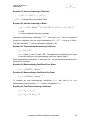
converted into engineering units in accordance to the calibration equation:
Equation 1 General Calibration Equation
LLightDat ( z , λ ) = ( LCountsLightDat ( z , λ ) − LCalDarkDat ( λ ) ) ⋅ a ( λ ) ⋅ ic( λ
)
where a is a calibration coefficient and ic is an immersion coefficient obtained from a
calibration file. To simplify notation, in the following dependence on wavelength ( λ ) will
be omitted. LCalDarkDat ⋅ a ⋅ ic is the dark current in engineering units that can be obtained
from a calibration file or using one of the dark current correction (DCC) methods
described below.
ProSoft currently implements DCC other than calibration dark or shutter dark only in
OPTIC1 (high resolution 24 bit systems) fitting mode (see SIFS for detailed explanation
of the fitting modes). Dark current can change under changing thermal conditions on
these high-resolution systems. Dark current correction has to be adjusted accordingly.
ProSoft provides the different DCC methods that will be described in the following
sections.
It is important to note that DCC other than based on the calibration file (except
hyperspectral) can only be used for the measurement frames obtained with gain switch 1
or higher in OPTIC1 fitting mode (in gain switch 0, or low gain, the CAL darks are used).
In OPTIC1 fitting mode, ProSoft first analyses the measured frames according to the
gain switches and applies the DCC according to the Dark Current Correction scheme
selected by the user. In OPTIC2 fitting mode there are only two options available, CAL
and NULL.
11.1.1.2 CAL darks
DCC method with calibration darks is given by the general calibration equation. This is
the default mode for both OPTIC1 and OPTIC2 data types.
11.1.1.3 NULL darks
NULL dark is a special mode in which no darks are subtracted during data calibration
(note that in the fitting mode OPTIC1, cal darks will be still subtracted for the frames with
gain switch 0).
Equation 2 NULL Dark
Copyright © 2004 by Satlantic Incorporated
30
ProSoft User Manual 7.7
SAT-DN-00228
LLightDat ( z , λ ) = LCountsLightDat ( z , λ ) ⋅ a ( λ ) ⋅ ic ( λ
)
11.1.1.4 BIN darks
If the profiler reaches a depth for which all the optical sensors reach their dark level, then
the darks can be computed from the average of a number of samples at the bottom of
the profile. For each wavelength λ, the value of DCC is obtained from a layer where
(
average minimum light values min LLightDat ( z , λ
)
) are observed.
Equation 3 BIN Dark
LLightDat ( z , λ ) = LLightDat ( z, λ ) − min LLightDat ( z , λ
)
z = z min ,..., z max
11.1.1.5 Dark Current Correction of hyperspectral (OPTIC3) Data
Usually hyperspectral data is dark corrected with the values obtained from shutter darks
to obtain the most accurate correction. Shutter darks are continuously recorded during
the measurements by occulting the input fiber with an optical shutter, typically after every
five light samples. Hyperspectral calibration and subsequent DCC is carried out in the
following steps:
1. Correct shutter dark counts obtained from a log file by dark offset (obtained as
the difference between shutter darks and capped darks).
Equation 4 Hyperspectral Dark
LCountsDarkDat = LCountsDarkDat − LCountsDarkOffset
2. Convert data counts into engineering units in accordance to the calibration
equations. The calibration equations for optical hyperspectral data is:
Equation 5 Hyperspectral Data Calibration
LLightDat = ( LCountsLightDat − LCalDarkDat ) ⋅ a ⋅ ic
it1
it 2
LDarkDat = ( LCountsDarkDat − LCalDarkDat ) ⋅ a ⋅ ic
it1
it 2
where a is the calibration coefficient, ic is an immersion coefficient, it1 is the integration
time during calibration and it2 is the integration time during the measurement. a, ic and
it1 are taken from a calibration file, it2 is obtained from the same log file as optical data.
3. Deglitch dark data using a first difference filter (optional).
4. Interpolate shutter darks as a function of measurement time to match the number
of dark and light data measurements.
5. Correct light data using shutter darks.
Equation 6 Hyperspectral Dark Correction
Copyright © 2004 by Satlantic Incorporated
31
ProSoft User Manual 7.7
SAT-DN-00228
L = LLightDat − LDarkDat
Note: SAS Instrument
GPS UTC time that was presented at Level 1a in HHMM (hours, minutes) format is
recalculated into seconds from the start of the current day. GPS date that was presented
at Level 1a in DDMMYY (day, month, year) format is recalculated into days since start of
the current year.
Note: Profiler
If one wants to use other than shutter dark (can be applied only to hyperspectral profiler)
correction (e.g. NULL) then AUTODARK settings should be changed for all profiler
sensor groups respectively i.e. one should change AUTODARK from SHUTTER to
NULL in the profiler sensor group that contains Lu as well as in the profiler group that
contains Ed. One will get wrong results if one group will have AUTODARK set to
SHUTTER, and the other group to NULL. However, one could use any of CAL, BIN, or
NULL dark corrections in any of the groups.
11.2 Level 1b – Level 2 Data Processing
All optical data sensors are checked for wavelength sequence. The columns of optical
data are organized from left to right as a function of the increasing wavelength.
Optical data can be also deglitched if respective settings in processing parameters are
set. As a rule the deglitching is not required.
11.2.1 Dark Data Deglitching
Optional deglitching module is applied to data to remove obvious glitches in dark data.
First, a first difference operator is applied to the time series of N frames of optical data at
each channel:
Equation 7 Dark Data Deglitching
dLλ ( i ) = Lλ ( i + 1) − dLλ ( i ) , i = 1,..., N − 1
Second, the standard deviation is calculated for each channel:
Equation 8 Standard Deviation
stdL( λ ) =
1 N−1
∑ ( dLλ ( i ) − dLλ
N − 2 i= 1
)
2
Third, any data which values are higher than 10 stdL ( λ
constant Nan.
)
is blanked by a blanking
11.2.2 Data Deglitching
This optional module can be toggled on/off using the processing parameters Deglitch
Profiler Data and Deglitch Reference Data. For details on how it works see
profiler/reference deglitching.
Copyright © 2004 by Satlantic Incorporated
32
ProSoft User Manual 7.7
SAT-DN-00228
11.2.3 Profiler Data Level 1b - Level 2 Processing
Profiler data has a number of corrections and checks before the level 2 data files are
created. These include pressure tare (offset) correction, wavelength sequence check
and a tilt quality control edit.
11.2.3.1
Pressure TARE Correction
Pressure sensors often have a small offset value that will change with atmospheric
pressure. The offset is removed by a pressure tare. This value is stored in the header
records by SatView when the data is collected. The pressure tare is defined as the
pressure value that is measured when a profiler's Ed sensor is located just at the
surface. This value has to be later subtracted from the measured pressure values of a
profile. If the profiler measurements were logged with SatView, the pressure tare value
is automatically inserted into the file header. If no information is obtained, pressure tare
value is set to 0.
11.2.3.2 Tilt Edit
Profiler measurements can be edited interactively or automatically removing any tilt
contaminated records. In manual mode, a plot is shown with profiler tilts (if available)
and profiler velocity as a function of depth. With the interactive graphical editor the user
defines an upper zmin and lower depth zmax (we assume that z co-ordinate is directed
downwards i.e. depth is zmin surface and zmax at the bottom of a profile). Data above zmin
or below zmax will be removed. A tilt Tilt ( z ) threshold Tiltlimit (default is 5 degrees) usually
is used for estimation of zmin and zmax. In a case of missing tilt sensor, the freefall velocity
of the profiler can be used (zero or negative velocity is assumed to be high tilt).
Automated editor module determines zmin and zmax in 10% of the upper and lower part of
profiler measurements. The upper depth and the lower depth are defined as the first
depth level (z) where the following conditions are met:
Tilt ( z ) < Tilt lim it
min( z ) ≤ z < 0.1 max( z ) for top layer of the profile
( max( z ) − 0.1 max( z ) ) < z ≤ max( z ) for bottom layer of the profile
If a reference instrument is present, then the matching records in the reference data are
also removed.
11.2.3.3 Reference Instrument
Reference data is checked before the level 2 data files are created. These checks
include wavelength sequence check and a spike deglitch.
Copyright © 2004 by Satlantic Incorporated
33
ProSoft User Manual 7.7
SAT-DN-00228
11.3 Level 2 – Level 3a Processing
Read Level 2 Data
Calculate Master Co-ordinates
Calculate Pressure
Co-ordinates
Calculate Time
Co-ordinates
Co-ordinate Interpolation
Write Level 2s File
Wavelength Interpolation
Natural Log Transform
Average Data
11.3.1 Read Level 2 Data
Data from the Level 2 hdf file is read and organized depending on the type of instrument
(i.e. Satnet Hyperspectral Profiler/Reference).
11.3.2 Calculate Master Co-ordinates
At level 3a processing, the averaging of data is done within intervals based on a system
of co-ordinates. For systems with a profiler the co-ordinates are based on pressure
(averaging in depth). For systems with a reference only or SAS the co-ordinates are
based on time (averaging in time).
Copyright © 2004 by Satlantic Incorporated
34
ProSoft User Manual 7.7
SAT-DN-00228
11.3.2.1 Calculate Pressure Co-ordinates
There exists in most instruments a difference in distance between sensors. For example
in an SPMR profiler the distance between the Ed sensor at the top and the Lu sensor at
the bottom is approximately 1.412 m. This presents a problem when defining a pressure
co-ordinate system that is common to all sensors that make up the instrument. When
processing optical data, the data closest to the surface is usually of greater importance
than data at the deepest of the profile. Therefore it makes sense to choose the sensor
nearest the surface which in all profiler cases is the Ed sensor. The pressure values for
the Ed sensor, hereafter referred to as master pressure, are then used to derive the
pressure co-ordinates. It should be noted that if no Ed sensor is present then the Lu
sensor pressure must be used instead.
The master pressure is then filtered to eliminate frames where pressure is not
increasing.
Equation 9 Pressure Filtering
depth(n + 1) − depth(n) ≤ 0
The pressure co-ordinates are created by rounding up the first master pressure value to
the nearest 0.1 m then increasing the pressure by intervals equal to the depth resolution
until reaching the highest (deepest) master pressure value which is rounded down to the
nearest 0.1 m. For example:
Master Pressure
From Ed
Pressure Coordinates
2.2657
2.3
2.3727
2.4
3.0684
2.5
4.2028
2.6
4.7808
etc.
5.4015
6.3
5.8510
6.4
6.3326
6.5
6.6323
6.6
11.3.2.2 Calculate Time Co-ordinates
Almost all reference instruments have an Es sensor which ProSoft uses to calculate the
time co-ordinate system. In the case of SAS instruments, an Lt sensor is always present
which is used to calculate the time co-ordinate system. There are three possible ways to
calculate the time values, hereafter referred to as master time, for each frame of the Es
or Lt sensor. They are listed below in order of precedence:
1. If a timer sensor is part of the instrument, then this is the most accurate way to
calculate the master time. The master time for the very first frame is taken as the first
Timetag2 value if available else Time Stamp, the time at which logging data begins, is
Copyright © 2004 by Satlantic Incorporated
35
ProSoft User Manual 7.7
SAT-DN-00228
used. The timer values give the elapsed time for each frame since the time of the first
frame which is used to calculate the absolute time for each frame. Note that timers are
available in Satnet systems as well as Hyperspectral systems.
2. If Timetag2 values were appended to the logged data then those values are used as
the absolute time for each frame.
3. The absolute time for the first frame is taken as the Time Stamp. The rate for the
sensor is then used to calculate the elapsed time for each frame which in turn is used to
calculate the absolute time for each frame.
The time co-ordinates are created by taking the first master time value and then
increasing it by an interval determined from the Es time data until reaching the last
master time value. For Sas data the time interval is determined from the optical sensor
operating at the fastest rate.
For example: (interval = 0.100 sec)
Master Time from Es
Time Co-ordinates
17:57:41.167
17:57:41.167
17:57:41.333
17:57:41.267
17:57:41.500
17:57:41.367
17:57:41.667
17:57:41.467
17:57:41.833
etc.
17:57:42.000
17:57:42.167
17:57:42.167
17:57:42.267
17:57:42.333
17:57:42.367
17:57:42.500
17:57:42.467
11.3.3 Coordinate Interpolation
The data to be averaged is interpolated onto the master co-ordinates ensuring that all
the data is mapped to a common co-ordinate system prior to averaging. The coordinates are based on either pressure or time. The interpolation method used for both
Profiler and Reference instruments is ‘linear’ and for SAS instruments ‘spline’ is used.
11.3.4 Write Level 2s HDF File
The interpolated data is written to the corresponding level 2s HDF file.
11.3.5 Wavelength Interpolation
Profiler, Reference and SAS data can be interpolated onto a constant wavelength
interval by setting the level 3 parameter Wavelength Interpolation to the desired interval.
Wavelength interpolation can only be used for Hyperspectral instruments. Multispectral
instruments have too few wavelength channels to provide an accurate interpolation. It is
highly recommended to use wavelength interpolation for Hyperspectral
Copyright © 2004 by Satlantic Incorporated
36
ProSoft User Manual 7.7
SAT-DN-00228
profilers/references as it will help maximize the number of matching wavelengths for
Level 4 processing.
11.3.6 Natural Log Transform
Optical sensor data (Lu, Es etc.) are natural log transformed to “straighten” the data prior
to averaging.
11.3.7 Average Data
The data is then averaged based on the level 3 parameters Bin Interval and Bin Width
for pressure co-ordinates and Time Interval and Time Width for time co-ordinates. The
Bin Interval or Time Interval determine the points at which to average with the Bin Width
or Time Width determining the number of data points to use for averaging.
For example: BIN_INTERVAL = 0.5 m BIN_WIDTH = 0.3 m
Copyright © 2004 by Satlantic Incorporated
37
ProSoft User Manual 7.7
SAT-DN-00228
11.4 Level 4 Data Processing
When using the level 4 processing menu a dialogue box allows the user to specify which
level 4 products to include in the level 4 HDF file. Each option selected will be included
as a separate sensor within the HDF file. The first two options, ‘Diffuse Attenuation
Coefficient’ and ‘Propagate Optical Variables to Surface’ are sometimes needed to
process other selections such as Water Leaving Radiance and will therefore be
automatically selected when needed.
Notes On Wavelength Differences: When processing calculations that involve data
from two different sources (e.g. comparing Lu and Ed sensors) the wavelengths from the
two sources will never be exact (e.g. Lu 489.8nm and Ed 490.1nm), unless wavelength
interpolation was selected at level 3a. Therefore ProSoft uses a matching tolerance
between wavelengths in order for the channels to be used in the calculation. For
example if Lu is 489.8nm and the closest Ed channel is 490.1nm (490.1 – 489.8 <
tolerance) these two channels can be used together in a calculation. In Level 4 data
presentation the wavelength shown is the mean value between the two wavelengths
(e.g. 489.95nm from the above example). Tolerances are set as follows, multispectral 2
nm and hyperspectral 0.5 nm.
11.4.1 Diffuse Attenuation Coefficient
Overview: Under typical conditions for which incident lighting is provided by sun and sky,
the various radiance and irradiance all decrease exponentially with depth, at least far
enough below the surface (and far enough above the bottom in shallow water) to be free
of boundary effects. This effect can be generally expressed as:
Equation 10 Diffuse Attenuation Coefficient (Ocean Optics Protocols for
SeaWiFS eqn. 26 pg. 49)
z
E d ( z , λ ) = E d ( 0 − , λ )e
Ed ( z, λ
(
)
− k d ( z ',λ ) dz '
∫
0
- downwelling irradiance as a function of depth and wavelength.
)
E d 0 − , λ - surface value of downwelling irradiance as a function of wavelength.
z
e
− k d ( z ', λ ) dz '
∫
0
- effect of the diffuse attenuation coefficient as a function of depth
and wavelength.
The traditional method of k analysis (Smith and Baker 1984 and 1986) is to estimate k(z)
as the local slope of measured ln(Ed(z)) in an interval of a few meters centered on depth
zm.
Equation 11 Ocean Optics Protocols for SeaWiFS eqn. 31 pg. 50
( ( ))
ln( E d ( z ) ) ≅ ln E d 0 − − ( z − z m ) k ( z m )
The slope k and the intercept Ed(0-) are calculated using a least squares regression fit of
the data over the number of regression points selected.
Copyright © 2004 by Satlantic Incorporated
38
ProSoft User Manual 7.7
SAT-DN-00228
p = polyfit( x, y, 1 ) MatLab function.
The degree of the resulting polynomial is one.
For the shallowest and deepest depths of a profile there is not enough data points to
meet the required number of points for regression. In this case the k value is calculated
by selecting the required number of points nearest to the depth upon which the k value is
centered. For example if 1m is the shallowest depth then the k value for 1m is based on
level 3a data taken from 1m to 3m, if Integration Points = 5, and the k value for 2m is
based on level 3a data taken from 1m to 4m. Therefore k values at the shallow and deep
sections of the profile are unreliable and are not used for Level 4 data calculations.
11.4.1.1 Integration Points
Integration points is the processing parameter that determines the number of data points
to use for regression analysis. Only odd number values can be used (e.g. 3,5, 7 etc.) in
order for depth z to be centered on the level 3a depth interval (e.g. 3m, 5m, 7m etc.).
Ed (uW/cm2/nm)
0m
Ed(0-)
1m
2m
Slope = K(3m)
INTEGRATION_POINTS = 5
3m
Depth 4 m
5m
6m
7m
8m
Slope = K(5m)
Note: Ed values are ln transformed prior to regression
analysis which would straighten out the curve.
Note: Successive values of K are calculated using
overlapping data points as can be seen in the above graph.
K Analysis
In cases where there is only a reference instrument and no profiler, therefore no K_Lu,
K_Ed or K_Eu, to propagate Ls to surface, then K is estimated from a time series of
upwelling radiance measured at a fixed depth below the surface. In this case ProSoft
estimates the spectrum of K(λ) in three steps:
1. Following the Austin Petzold (1981) model, K is estimated at the wavelengths
443nm and 550nm.
Equation 12 Austin Petzold 490nm
Copyright © 2004 by Satlantic Incorporated
39
ProSoft User Manual 7.7
SAT-DN-00228
K ( 490 ) =
 Lu ( 443) 

0.0833
 Lu ( 550 ) 
− 1.491
+ 0.022
Equation 13 Austin Petzold 520nm
 Lu ( 443) 

K ( 520 ) = 0.0663
 Lu ( 550 ) 
− 1.398
+ 0.044
These K values are used in step 2 to obtain the concentrations of pigments C at
490nm and 520nm.
2. Morel’s (1988) empirical model for estimation of K is inverted to obtain the
concentration of pigments (Chl a and Pheo):
Equation 14 Morel 1988
 K(λ ) − Kw (λ
C = 
χc

Kw(λ
)
- diffuse
MORELKW.FIT
χ
c
e( λ
(λ )
)
1
)  e ( λ )


attenuation
coefficient
of
water.
Obtained
from
file
- coefficient determined empirically. Obtained from file MORELCHI.FIT
- coefficient determined empirically. Obtained from file MORELEPS.FIT
C is obtained as the average value of the two C’s calculated at 490nm and
520nm and is used in step 3.
3. The spectrum of K(λ) is obtained using Morel’s equation 9 (1988):
Equation 15 Morel 1988 Equation 9
Kap ( λ ) = K w ( λ ) + χ ( λ ) C e ( λ )
To calculate Kap within 700-800nm, ProSoft uses the following steps:
i. The values of Kw(λ) within 700-800nm are obtained from Smith and Baker (1981)
MORELKW.FIT.
ii. It is assumed that χ(λ) and e(λ) decrease linearly from the values given at χ(700)
and e(700) to 0 and 800nm respectively.
iii. Using the above assumption and Kw within 700-800nm, K(λ) can be estimated at λ
= 700-800nm interval.
The K values calculated depend on the instrument configuration. Possible values are:
K_Ed
K_Lu
K_Eu
Kap_Ls – K is calculated using the Austin Petzold model
Copyright © 2004 by Satlantic Incorporated
40
ProSoft User Manual 7.7
SAT-DN-00228
11.4.2 Propagate Optical Variables to Surface
The surface values of the profiler optical variables are obtained as the intercept of a
least squares regression fit based on the shallowest depth centered on Zm.
Equation 16 Surface Variables (Ocean Optics Protocols for SeaWiFS eqn.
31 pg. 50)
( ( ))
ln( E d ( z ) ) ≅ ln E d 0 − − ( z − z m ) K ( z m )
The calculated intercept is a product of the diffuse attenuation coefficient (Kd)
calculation. As a result, if optical variables are propagated to the surface, the Kd profile
for each optical variable (Lu, Ed and Eu) will be calculated and included with the level 4
hdf file. In cases of shallow depths that do not meet the required number of points for
regression, the surface variable is calculated based on the intercept of the k slope from
the first depth value that has the required number of points. For example in k analysis
the surface optical variable Ed(0-) will be calculated on the intercept of the slope based
on the k value at 3m and not at 1m or 2m.
Possible values include:
Profiler:
Ed(0-) calculated from K_Ed
Lu(0-) calculated from K_Lu
Eu(0-) calculated from K_Eu
Reference:
Es(0-) if Es is measured above the surface then Es(0-) is calculated using:
Equation 17 Es(0-)
( )
Es 0− =
Es ( λ )
1+ α
α – Fresnel reflection albedo for irradiance from sun and sky. Default
value of 0.043 which can be changed as a level 4 parameter.
Ls(0-) is calculated using one of the following (whichever one is available
starting with the top):
K_Lu
K_Ed
K_Eu
Kap_Ls – K is calculated using the Austin Petzold model
Example:
Equation 18 Ls(0-)
Ls (0 − , λ ) = Ls ⋅ e z ⋅ k
Copyright © 2004 by Satlantic Incorporated
41
ProSoft User Manual 7.7
SAT-DN-00228
11.4.2.1 Reflection Albedo
Processing parameter that sets the value for the Fresnel reflection albedo for irradiance
from sun and sky. A default value of 0.043 is used and can be changed as a level 4
processing parameter.
11.4.3 Water Leaving Radiance
Normalized water leaving radiance is estimated with the following equation:
Equation 19 Normalized Water Leaving Radiance (Ocean Optics Protocols
eqn. 63 pg. 54)
Lwn = Lw ( λ
)
Fo ( λ
Es ( λ
)
)
Fo(λ) – the mean extraterrestrial solar irradiance (Neckel and Labs 1984)
Es(λ) – downwelling spectral irradiance at z(0+)
Lw(0+,λ) – upwelling radiance propagated through the surface z(0+) using:
Equation 20 Water Leaving Radiance
(
)
(
Lw 0 + , λ = Lu 0 − , λ
) 1 − ρ ( λ ,θ )
η
2
w
(λ )
ρ(λ,θ) – Fresnel reflectance index of seawater. Default value of 0.021 for seawater
which can be changed as a level 4 global variable.
ηw(λ) – Fresnel refractive index of seawater. Default value of 1.345 for seawater
which can be changed as a level 4 global variable.
Es(λ) from water leaving radiance is usually obtained from an above water reference, but
in cases where no reference data is available Ed(0-,λ), measured by a profiler, is used.
Ed is extrapolated through the surface using:
Equation 21 Ed(0+)
(
)
(
)
E d 0 + , λ = E d 0 − , λ (1 + α
)
α – Fresnel reflection albedo for irradiance from sun and sky. Default value of 0.043
is used which can be changed as a level 4 processing parameter.
If Lu(0-,λ) from water leaving radiance is not available then Ls(0-,λ) is used instead. Ls(0,λ) is calculated when propagating variables to the surface.
The values used for Fo(λ) (Neckel and Labs) can be found in the file Solar10.dat.
11.4.3.1 Reflectance Index
Fresnel reflective index for seawater. A default value of 0.021 is used and can be
changed as a level 4 processing parameter.
Copyright © 2004 by Satlantic Incorporated
42
ProSoft User Manual 7.7
SAT-DN-00228
11.4.3.2 Refractive Index
Fresnel refractive index for seawater. A default value of 1.345 is used and can be
changed as a level 4 processing parameter.
11.4.4 Surface Remote Sensing Reflectance's
Remote sensing reflectance's RL(0+,λ) are calculated using:
Equation 22 Surface Remote Sensing Reflectance
(
(
LW 0 + , λ
RL 0 , λ =
Ed 0 + , λ
(
+
)
)
)
Ed(0+,λ) – denotes downwelling spectral irradiance measured just above the surface
(Es) or extrapolated through the surface Ed(0+). For Es the median of the time
series data is taken for each wavelength.
Lw(0+,λ) – denotes upwelling spectral radiance propagated through the surface.
The remote sensing reflectance's calculations produce several possible combinations
depending on the instrument configuration. Possible values include:
i. for Lu and Ed sensors Lu(0+,λ)/Ed(0+,λ)
ii. for Lu and Es sensors Lu(0+,λ)/Es(λ)
iii. for Ls and Es sensors Ls(0+,λ)/Es(λ)
Ed is extrapolated through the surface using:
Equation 23 Above Surface Ed(0+)
(
)
(
)
E d 0 + , λ = E d 0 − , λ (1 + α
)
α – Fresnel reflection albedo for irradiance from sun and sky. A default value of
0.043 is used and can be changed as a level 4 processing parameter.
Lw is calculated using:
Equation 24 Water Leaving Radiance
(
)
(
Lw 0 + , λ = Lu 0 − , λ
) 1 − ρ ( λ ,θ )
η
2
w
(λ )
ρ(λ,θ) - Fresnel reflectance index of seawater. Default value of 0.021 is used.
ηw(λ) - Fresnel refractive index of seawater. Default value of 1.345 is used.
11.4.5 Remote Sensing Reflectance Profile
Remote sensing reflectance profile is calculated as the ratio of upwelling radiance to
downwelling irradiance with changing depth. Only Lu is used for upwelling radiance and
Ed for downwelling irradiance.
Equation 25 Remote Sensing Reflectance Profile
Copyright © 2004 by Satlantic Incorporated
43
ProSoft User Manual 7.7
SAT-DN-00228
RSR =
Lu ( z, λ )
Ed ( z, λ )
11.4.6 Surface Reflectance's
Surface reflectance is calculated as the ratio of upwelling irradiance just above the
surface to downwelling irradiance just above the surface.
Upwelling irradiance can be derived from several sources depending on the instrument
configuration and include Eu(0+), Lu(0+) converted to Eu(0+), Ev(0+) and Ls(0+) converted
to Ev(0+).
Downwelling irradiance can be derived from several sources depending on instrument
configuration and include Ed(0+) and Es.
Equation 26 Surface Reflectance
RFL =
(
)
Upwelling _ Irradiance 0 + , λ
Downwelling _ Irradiance 0 + , λ
(
)
The following sensor combinations are possible:
i. Eu and Ed sensors: Eu and Ed are propagated above the surface using
Equation 27 Above Surface Ed(0+)
(
)
(
)
E d 0 + , λ = E d 0 − , λ (1 + α
)
α – surface albedo (default = 0.043)
RFL = Eu(0+,λ)/Ed(0+,λ)
ii. Lu and Ed sensors: Lu is propagated above the surface and converted to Eu using:
Equation 28 Above Surface Eu(0+)
(
)
(
Eu 0 + , λ = 4.5 ⋅ Lu 0 − , λ
) 1 − ρ ( λ ,θ )
η
2
w
(λ )
ρ – reflective index (default = 0.021)
ηw – refractive index (default = 1.345)
RFL = Eu(0+,λ)/Ed(0+,λ)
iii. Lu and Es sensors: Lu is propagated above the surface and converted to Eu using
equation Eu(0+,λ).
RFL = Eu(0+,λ)/Es(λ)
iv. Ev and Es sensors : Ev is propagated above the surface using equation Ed(0+,λ).
RFL = Ev(0+,λ)/Es(λ)
v. Ls and Es sensors: Ls is propagated above the surface and converted to Ev using
equation Eu(0+,λ).
RFL = Ev(0+,λ)/Es(λ)
Copyright © 2004 by Satlantic Incorporated
44
ProSoft User Manual 7.7
SAT-DN-00228
11.4.7 Reflectance Profile
The reflectance profile is calculated as the ratio of upwelling irradiance to downwelling
irradiance. The most preferred method of calculation is to use upwelling irradiance Eu
from the profiler and downwelling irradiance Ed, also from the profiler.
Equation 29 Reflectance Profile
RFL =
Eu ( z, λ )
E d ( z, λ )
11.4.8 Photosynthetically Available Radiation
Photosynthetically available radiation is a measure of the number of photons available
for photosynthesis by chlorophyll. Units of PAR are expressed as quanta/cm2s and is
estimated using the following:
Equation 30 Photosynthetically Available Radiation
700 nm
PAR =
λ
E d ( λ ) dλ
hc
400 nm
∫
λ – wavelength
h – Planck’s constant 6.625x10-34 Js
c – speed of light 3x108 m/s
Ed(λ) – downwelling spectral irradiance (µW/cm2 /nm)
Prior to integration Ed(λ) is interpolated onto a constant 1nm interval and subject to the
following rules:
if λ1 > 400nm then Ed(400) = Ed(λ1)
if λn < 700nm then Ed(700) = Ed(λn)
Included with the PAR data is the percentage of PAR for various depths. This ratio is
calculated as:
Equation 31 Percentage PAR
PAR( z )
PAR 0 +
% PAR =
( )
The attenuation coefficient of PAR (K_PAR(0-)) is also calculated near the surface using
the same methods as described under the diffuse attenuation coefficient. This value is
included in the data table attributes as K_PAR(0-).
If reference Es data is available then PAR is calculated as:
Equation 32 Reference Par
700 nm
PAR =
λ
E s ( λ ) dλ
hc
400 nm
∫
Copyright © 2004 by Satlantic Incorporated
45
ProSoft User Manual 7.7
SAT-DN-00228
The median value of PAR is then calculated and included in the vdata table attributes
and called Reference PAR.
11.4.9 Chlorophyll a Profile Estimates Morel 98 Model
The estimation of chlorophyll a concentration (µg/l) in profile is estimated for each depth
level given from the level 3a hdf file. The method used is as follows:
Equation 33 Morel 98 Chlorophyll Model
 K ( λ ) − KW ( λ
C = 
χ C (λ )

) 
1
e( λ
)


χC, KW and e(λ) are taken from the Morel 98 model. These values can be seen in the files
MOR98CHI.DAT, MOR98KW.DAT and MOR98EPS.DAT located in the ProSoft
installation directory.
The Morel 98 model is derived from equation 9 pg. 10753 from:
“Optical Modeling of the Upper Ocean in Relation to Its Biogenous Matter Content”
Andre Morel
Journal of Geophysical Research Volume 93 No. C9, pg. 10749-10768
11.4.10 Chlorophyll a Surface Estimates SeaBAM OC2 Model
Chlorophyll a concentration is estimated at the water surface using the remote sensing
reflectance values calculated previously.
Equation 34 Chlorophyll a Surface Estimate SeaBAM OC2 Model
C = 10 ( 0.2974− 2.2429 R + 0.8358 R
2
− 0.0077 R 3
) − 0.0929
Equation 35 Calculation of R Coefficient
(
R = Log10 Rrs 490nm
Rrs555nm
)
The calculation of R coefficient uses the remote sensing reflectance values at 490nm
and 555nm to calculate the value of R. Therefore several different calculations of
Chlorophyll a are possible depending on how the remote sensing reflectance was
calculated. The possible combinations are Lu(0+)/Es, Lu(0+)/Ed(0+) and Ls(0+)/Es.
The value of R is then used in to calculate the chlorophyll a concentration (µg/l) at the
surface.
Equations for chlorophyll a surface estimate and calculation of R coefficient are derived
from:
“Ocean Color Chlorophyll Algorithms for SeaWiFS”
O’Reilly et al.
Journal of Geophysical Research, Volume 103, No. C11, pg. 24937-24953
Copyright © 2004 by Satlantic Incorporated
46
ProSoft User Manual 7.7
SAT-DN-00228
11.4.11 Chlorophyll a Surface Estimates Gordon 88 Model
Chlorophyll a concentration is estimated at the water surface using the normalized water
leaving radiance's calculated previously.
Equation 36 Chlorophyll a Surface Estimate Gordon 88 Model
(
C = 1.15 Lwn 443nm
)
Lwn560nm
− 1.42
C ≤ 1µ g
l
Equation 37 Chlorophyll a Surface Estimate Gordon 88 Model
(
C = 3.64 Lwn500nm
)
Lwn560nm
− 2.62
C > 1µ g
l
The equations for Chlorophyll a surface estimate use normalized water leaving
radiance's values at 443nm, 500nm and 560nm. Therefore several different calculations
of chlorophyll a are possible depending on how the normalized water leaving radiance
was calculated. The possible combinations are Lu(0+)/Ed(0+), Lu(0+)/Es and Ls(0+)/Es.
Equations for Chlorophyll a surface estimates are taken from:
“Ocean Color Remote Sensing Systems: Radiometric Requirements”
H. Gordon
Processing for Remote Sensing, pg. 151-167
11.4.12 Estimation of Energy Fluxes
Energy fluxes are estimated using the following equation:
Equation 38 Estimation of Energy Fluxes
700
F = 100 ∫ Ed ( λ ) dλ
400
ProSoft uses Matlab’s trapezoidal numerical integration routine ‘trapz.m’ to perform the
integration. Prior to integration, a minimum-maximum wavelength check is performed
then the irradiance data is interpolated onto a constant 1nm interval. Since irradiance
data is measured in units of μWcm-2nm-1, a scaling factor of 100 is used to convert from
cm-2 to m-2.
11.4.13 Backscattering Coefficients
Backscattering values are derived from an ECO Series IOP instrument which contains a
scattering meter to measure backscattering at 117 degrees within a volume of water.
β (117  , λ
)
Values represent total volume scattering as measured by the instrument. To
obtain the volume scattering of particles only, subtract the volume scattering of water,
β w 117  , λ from the total volume scattering:
(
)
Copyright © 2004 by Satlantic Incorporated
47
ProSoft User Manual 7.7
SAT-DN-00228
Equation 39 Volume Scattering of Particles
(117 , λ ) = β (117 , λ ) − β (117 , λ )
(117 , λ ) is obtained from (from Morel 1974):
β
β
ρ



w

w
Equation 40 Volume Scattering of Water
β
w
(θ , λ ) = 1.38( λ
/ 500nm )
− 4.32
(1 +
(
)
0.3S / 37 )10 − 4 1 + cos 2 θ (1 − δ ) / (1 + δ ) m − 1 sr − 1
δ = 0.09
S = Salinity obtained from water properties
Particulate backscattering coefficients, bbp ( λ
)
with units of m-1, can be determined
through an estimation from the single measurement of β
(117 , λ )

p
using an X factor.
This factor estimates bbp with an estimated uncertainty of 4%.
Equation 41 Particulate Backscattering Coefficient
bbp = 2π Xβ
(117 )

p
X = 1.1 (Boss, E, and S. Pegau, 2001. The relationship of scattering in an angle
in the back direction to the backscattering coefficient, Applied Optics)
Water backscattering coefficients, bw with units of m-1 can be determined by either of the
following two equations:
Equation 42 Backscattering Coefficient Pure Water
bw ( λ ) = 0.0022533( λ / 500nm )
− 4.23
Equation 43 Backscattering Coefficient Sea Water
bsw ( λ ) = 0.0029308( λ / 500nm )
− 4.24
To compute the total backscattering coefficients, bb ( λ
backscattering from pure water, bbw ( λ
)
)
with units of m-1, the
needs to be added to bbp ( λ ) :
Equation 44 Total Backscattering Coefficient
bb ( λ ) = bbp ( λ ) + bbw ( λ
)
bbw ( λ ) = bw ( λ ) / 2 or bsw ( λ ) / 2
Copyright © 2004 by Satlantic Incorporated
48
ProSoft User Manual 7.7
SAT-DN-00228
12. Appendix A: Term Definitions
12.1 File Naming Convention
HDF File – ProSoft input or output data file where meta-information and data have been
organized using Hierarchical Data Format following the principles of data organization
and processing.
Instrument File – a calibration (*.cal) file or a telemetry definition file (*.tdf) ( for details
see Satlantic Instrument File Standard).
File Nametag – last letters or numbers which follow underscore ('_') in a file name.
Level 1 – binary logged data file with the RAW extension.
Level 1a – binary data is extracted from RAW data under the control of the instrument
(calibration) files. Extracted information is grouped along with its calibration information
and placed into Level 1a hdf files. File nametag is _L1a.
Level 1b – Level 1a data is calibrated. No data editing is applied. Shutter darks, if
present, are not applied. File nametag is _L1b.
Level 2 – includes Level 1b data, which is further modified per request basis. File
nametag is _L2.
1. Shutter dark correction is applied; reference and dark data deglitching is applied.
2. Profiler's data is tilt edited
Level 2s – level 2 data is interpolated onto a common co-ordinate vector, which is either
depth (Profiler) or time (Reference only or Sas). File nametag is _L2s.
Level 3a – Averages level 2s data as defined by level 3 processing parameters
Level 4 – Data products produced from level 3a data.
12.2 Optical Sensors
Ed - Profiler downwelling plane irradiance
Lu - Profiler upwelling radiance
Eu - Profiler upwelling plane irradiance
Ld - Profiler downwelling radiance (special applications only)
Es - Reference downwelling plane irradiance
Ls - Reference upwelling radiance
Ev - Reference upwelling plane irradiance
Ef - Reference downwelling plane diffuse irradiance (special applications only)
Li - SAS sky radiance
Lt – SAS water leaving radiance
Units: Irradiance - µW/cm2/nm
Radiance - µW/cm2/nm/sr
Copyright © 2004 by Satlantic Incorporated
49
ProSoft User Manual 7.7
SAT-DN-00228
12.3 Ancillary Sensors
Tw
- External water temperature (oC)
Ti
- Internal irradiance sensor array temperature (oC)
Tr
- Internal radiance sensor array temperature (oC)
Pres - Profiler depth (m)
TiltX - Sensor tilt on X axis (deg)
TiltY - Sensor tilt on Y axis (deg)
Rtilt - Reference tilt about vertical axis (deg)
Ptilt - Profiler tilt about vertical axis (deg)
Pitch - Sensor tilt along horizontal axis (deg)
Roll - Sensor tilt about horizontal axis (deg)
Cond - Seawater conductivity (mmho/cm)
Fluor - Fluorometer (µg/l)
Trans - Transmissometer (/m)
Comp - Flux gate compass (deg)
Altim - Altimeter (distance from bottom) (m)
PAR
- PAR sensor (µE/m2)
Time - system time (decimal hours)
Vel
- profiler descent velocity (m/sec)
Frame - Instrument frame counter (0..255)
LuDark - Profiler radiance dark detector OCR-1000 only (counts)
EdDark - Profiler irradiance dark detector OCI-1000 only (counts)
EsDark - Reference irradiance dark detector OCI-1000 only (counts)
LsDark - Reference radiance dark detector OCR-1000 only (counts)
Copyright © 2004 by Satlantic Incorporated
50
ProSoft User Manual 7.7
SAT-DN-00228
13. Appendix B: Data Formats
Table 1 File Header
File Header
Units
Description
PROSOFT
None
ProSoft software version used in analysis
CRUISE-ID
None
Identifies the cruise on which the current
series of log files is taken.
OPERATOR
None
Identifies the operator of the data
acquisition software for the current log
file.
LATITUDE
Decimal
Degrees
Identifies the latitude coordinates of the
instrument for the current log file.
LONGITUDE
Decimal
Degrees
Identifies the longitude coordinates of the
instrument for the current log file.
ZONE
None
Identifies the data acquisition time zone
of the current log.
COMMENT
None
Comment field for ancillary sky and sea
observations
STATION-ID
None
Identifies the station for the current
series of log files.
CAST
None
Identifies the current log file in a series of
related log files.
TIME-STAMP
None
Identifies the time on the data acquisition
computer as of the beginning of the
current log file.
MODE
None
Identifies the data acquisition software
mode.
PRESSURE-TARE
Meters (m)
Pressure tare taken at the surface for
current log file.
TIMETAG
None
Obsolete.
DATETAG
(YYYYDDD)
Switch to include date/time tagging.
TIMETAG2
(HHMMSSsss)
Switch to include timetag2 tagging.
PROFILER
None
Identifies the status
instrument.
REFERENCE
None
Identifies the status of the reference
instrument.
PRO-DARK
None
Profiler dark correction method.
REF-DARK
None
Reference dark correction method.
PRO-ID
None
This field is the identifier for the profiler.
PROCESSING_LEVEL
None
Identifies the processing level of the
current file.
Copyright © 2004 by Satlantic Incorporated
of
the profiler
51
ProSoft User Manual 7.7
SAT-DN-00228
FILE_CREATION_TIME
None
Date of file creation.
DEGLITCH_PRODAT
None
Switch to include deglitching of profiler
data.
DEGLITCH_REFDAT
None
Switch to include deglitching of reference
data.
PRESS_TARE_CORRECTION
Meters (m)
Pressure tare value applied to current log
file.
DEPTH_RESOLUTION
Meters (m)
Depth resolution used for Level 2s data
interpolation.
BIN_INTERVAL
Meters (m)
Level 3a variable that determines which
depth interval to average.
BIN_WIDTH
Meters (m)
Level 3a variable that determines depth
range within which to average.
TIME_INTERVAL
Seconds
Level 3a variable that determines which
time interval to average.
TIME_WIDTH
Seconds
Level 3a variable that determines the
time range within which to average.
WAVEL_INTERP
(nm)
Level 4 variable that determines
wavelength interpolation interval.
INTEGRATION_POINTS
None
Level 4 variable that determines number
of data points to use for regression
analysis.
REFLECTION_ALBEDO
None
Reflection albedo value used in level 4
processing.
REFLECTANCE_INDEX
None
Reflectance index value used in level 4
processing.
REFRACTIVE_INDEX
None
Refractive index value used in level 4
processing.
Table 2 Level 1-2 Table Descriptors
Table Label
Units
Description
PRES
Meters (m)
Used to define a pressure sensor measurement.
Pressure measurements are usually used with
submersible instruments to gauge their depth.
ALTIM
Meters (m)
Used to define an altimeter sensor measurement.
Altimeter measurement is normally used to gauge the
distance from a submersible instrument to the ocean
floor.
FRAMECOUNTER
None
The value of a frame counter is simply a numerical
counter that can help ensure all frames received are
sequential.
CHECKSUM
None
The value of the check sum is the last byte of the sum of
all bytes, up to but not including the check sum sensor, in
a frame of telemetry subtracted from 0.
Copyright © 2004 by Satlantic Incorporated
52
ProSoft User Manual 7.7
SAT-DN-00228
INTTIME
Seconds
Defines the adaptive or adjusted integration time for all
subsequent optical sensors for which the sensor was
defined.
DARK
None
Some optical sensors are shielded from light exposure to
establish a dark noise floor for a related optical sensor
grouping.
DARK_SAMP
None
Indicates the number of dark sensors used to calculate a
dark average.
DARK_AVE
None
Defines the actual average dark value.
T
Degrees
Celsius (°C)
Used to define a temperature sensor measurement.
Temperature sensors can be placed anywhere on an
instrument.
TILT
Degrees
Used to define a tilt or attitude measurement for an
instrument. A tilt measurement is normally used to
determine the alignment of an instrument with the
vertical.
PITCH
Degrees
Used to define a tilt sensor along the horizontal axis. A
pitch sensor can be used to determine an instruments
orientation relative to the horizon.
ROLL
Degrees
Used to define a tilt sensor about the horizontal axis. A
roll sensor can be used to determine an instruments
orientation relative to the horizon.
COMP
Degrees
Used to define a flux gate compass sensor
measurement. These sensors measure magnetic flux to
establish a compass direction.
COND
(mmho/cm)
Used to define a seawater conductivity sensor
measurement. A conductivity measurement is necessary
for calculation of salinity.
FLUOR
(µg/l)
Used to define a Fluorometer sensor measurement.
TRANS
(/m)
Used to define a Transmissometer sensor measurement.
A Transmissometer measurement indicates the
attenuation of a light beam in a given media.
PAR
(µE/m2)
Used to define a sensor for measuring photosynthetically
active radiation. PAR measurements indicate the total
light energy available for photosynthesis per unit area.
TIMER
Seconds
Used to define a timer sensor for indicating the number of
seconds that have elapsed since the instrument was
powered up.
Table 3 GPS Table Descriptors
Table Label
Units
Description
UTCPOS
None
Used to define the Universal Coordinated Time of the GPS frames
LATPOS
Degrees
Used to define the latitude coordinates of the GPS frames.
Copyright © 2004 by Satlantic Incorporated
53
ProSoft User Manual 7.7
SAT-DN-00228
LONPOS
Degrees
Used to define the longitude coordinates of the GPS frames.
LATHEMI
None
Used to define the hemisphere of the associated latitude
coordinates.
LONHEMI
None
Used to define the hemisphere of the associated longitude
coordinates.
SPEED
Knots
Used to define the ground speed of the GPS frames.
COURSE
Degrees
Used to define the course over the ground in degrees true.
MAGVAR
Degrees
Used to define the magnitude of the magnetic variation to be used
between true and magnetic degrees.
DATE
None
Used to define the date of the GPS measurements (ddmmyy)
MODE
None
Used to define the position system mode for the GPS sensor (i.e.
A = Autonomous, D = Differential)
Table 4 Level 4 Table Descriptors
Table Label
Units
Description
K_Lu , K_Ed, K_Eu
(/m)
K values
Lu(0-), Ed(0-), Eu(0-), Es(0-)
(µw/cm2/nm) or (µw/cm2/nm/sr)
Surface optical data
Lw-Lu(0+), Lw-Ls(0+)
(µw/cm2/nm/sr)
Water leaving radiance.
(µw/cm2/nm)
Normalized
water
leaving radiance.
RSR-Lu(0+)/Ed(0+), RSR-Lu(0+)/Es,
RSR-Ls(0+)/Es
(/sr)
Surface remote sensing
reflectance.
RSR-(Lu/Ed)
(/sr)
Remote
sensing
reflectance profiles.
RFL-Eu(0+)/Ed(0+), RFL-Eu(0+)/Es
(/sr)
Surface reflectance’s.
Profiler Par
(µMol/m2/s)
Photosynthetically
available radiation
Morel
98
Chlorophyll
Profile,
SeaBAM OC2 Surface Chlorophyll,
Gordon 88 Surface Chlorophyll
(µg/l)
Chlorophyll Estimates
Profiler Flux, Reference Flux
(w/m2)
Energy fluxes
Water Properties Table
Depth (m)
Water Properties
Lwn-Lu(0+)/Ed(0+),
Lwn-Ls(0+)/Es
Lwn-Lu(0+)/Es,
Temp (°C)
Conductivity (µmho/cm)
Conductivity Ratio (None)
Salinity (psu)
Density (Kg/m3)
Copyright © 2004 by Satlantic Incorporated
54
ProSoft User Manual 7.7
SAT-DN-00228
14. Appendix C: Profiler/Reference Data Deglitching Function
14.1 Background
Deglitching of optical data measured in sea environment is not a trivial task. Data
glitches that can be caused by power instabilities, inconsistencies between data transfer
baud rates and data logging speed, and other reasons that are not caused by changes
in the natural environment. On the other hand, noise in optical data can be also be
caused by wave-focusing effects, random changes in profiler's tilts, and the noise
caused by dark current.
We make difference between the data glitches and remaining part of unwanted noise
mainly to make possible differential data treatment depending on the cause of a noise. In
a case of glitches, we want the respective part of data simply removed. In a case of
wave focusing, dark current (DC) influence and profiler tilts, one may try to reduce their
influence by some sort of data filtering. In an extreme case, data with significant tilts, DC
etc can be also removed.
14.2 Description of data distribution with depth
1. Profiler's optical data changes exponentially with depth. Changes in signal values can
be as large as 8 orders e.g. from 1 to 1e-8.
2. Part of the data changes that can be regarded as noise, also change significantly.
Moreover, noise distribution with depth is not homogenous. The causes for noise in the
different parts of a profiler are different e.g. if in the surface layer wave focussing and tilt
effects are dominating then with the depth increase, dark current noise contribution
increases, and finally starts to dominate.
14.3 Problem
To identify glitches, one should divide measured data profile (S) into two parts: signal
(<S>) and noise (E).
S= S + E
(1)
where operator <> means some sort of data averaging. From equation (1) it is clear that
noise definition E = S − S depends on a meaning of operation of data averaging. The
measurements with E > Threshold will be declared glitches. Mean signal <S> can be
estimated using various approaches. E.g. FFT, wavelet transform, measured data fit with
a semi-empirical or empirical model (e.g. simple exponential or polynomial fit), simple
moving average etc. In all these cases, distribution of E with depth will remain
statistically inhomogeneous i.e. one could expect that p.d.f of E will change as a function
of depth. The outlined inhomogeneous error distribution constitutes the main
problem for glitches identification and their subsequent removal.
14.4 Approach for the Problem Solution
1. We assume that we have data S measured at fixed time or depth interval. For
simplicity we will use data frame number 'i' instead of a time or space co-ordinate. Thus
we have
Copyright © 2004 by Satlantic Incorporated
55
ProSoft User Manual 7.7
SAT-DN-00228
S(i), where i = 1,…, N, where N is number of measurements
2. From S(i) we calculate the ratio
dS(i) = S(i+1)/S(i), i = 1, …, N-1
3. Sort dS in an ascending order
dS_sorted = sort(dS)
4. Calculate a measure of data deviation
stdS = dS_sorted(n1) - dS_sorted(n2), where
n1 = 0.2*nn
n2 = 0.75*nn
nn = length of dS
5. Calculate median value of dS
medN = median(dS)
6. Find data invalid data values
| dS(i) – medN | > NoiseThresh*stdS
The default values for a profiler and a reference instrument are 5 and 20 respectively.
They should be adjusted according to a concrete situation.
From Step 6 it follows that all values that lie above NoiseThresh*stdS, should be
removed.
14.5 Examples
Figures 1 and 2 show the examples of measured upwelling radiance signal Lu without
glitches (Figure 5b) and with glitches (Figure 6b). The position of the vertical red lines in
the figures 1a, 1c and 2a indicate the levels below or above which data will be declared
as a glitch. Figure 5 shows data that had not any glitches in a sense defined above.
However, one can see that significant part of data dominated by dark noise at the bottom
of the profile is declared as the glitches. Although, usually this is not a problem to reject
data dominated by DC, the given example demonstrates a potential problem in making
difference between different causes of noise. In some cases wave focussing effects
(practically not visible in the present examples) are also clearly visible in the upper part
of a profile, and can be easily misinterpreted by a program as glitches in data. For this
reason, sometimes it could be advantageous to perform data deglitching analysis only to
some parts of a profile by identifying upper and lower depth boundaries of a profile. The
deglitching function appended to this document enables a user to define the respective
boundaries using ProSoft’s configuration file (see the last section of this note). In this
way, depending on an aim of deglitching analysis, one could also remove or not touch
significant amount of data affected dark noise or wave focusing.
Copyright © 2004 by Satlantic Incorporated
56
ProSoft User Manual 7.7
SAT-DN-00228
Figure 8 Distribution of upwelling Lu radiance
with depth with no data glitches. (a) Distribution ratio of Lu(i+1)/Lu(i), two vertical red
lines stay for medN | +/- NoiseThresh*stdS, (b) distribution of Lu as a function of
pressure, (c) and (d) – the same as (a) and (d) but for downwelling irradiance.
L u (i+ 1 )/ L u (i)
M e a s u re d L u 4 1 2 . 4
0
-2 0
-4 0
-5 0
-6 0
-8 0
P re s s u re / d b a rs
P re s s u re / d b a rs
-1 0 0
-1 0 0
-1 2 0
-1 5 0
-1 4 0
-1 6 0
-2 0 0
-1 8 0
-2 0 0
0.5
1
1 .5
-2 5 0
-8
-6
-4
-2
0
2
L o g (L u )
Copyright © 2004 by Satlantic Incorporated
57
ProSoft User Manual 7.7
SAT-DN-00228
Figure 9 The same as Figure 5 (a) and (b) but with apparent data glitches.
(c) distribution of deglitched Lu as a function of depth.
M e a s u re d L u 4 4 2 . 8
0
-1
-1
-2
-2
-3
-3
P re s s u re / d b a rs
P re s s u re / d b a rs
L u (i+ 1 )/ L u (i)
0
-4
-4
-5
-5
-6
-6
-7
-7
-8
-2 0
-1 0
0
10
20
-8
-6
-5
-4
-3
-2
L o g (L u )
Copyright © 2004 by Satlantic Incorporated
-1
0
1
58
ProSoft User Manual 7.7
SAT-DN-00228
M e a s u re d L u 4 4 2 . 8
-1
-2
P re s s u re / d b a rs
-3
-4
-5
-6
-7
-8
-5 . 5
-5
-4 . 5
-4
L o g (L u )
Copyright © 2004 by Satlantic Incorporated
-3 .5
-3
-2 .5
59