1
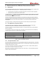
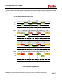
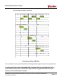
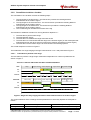
APPLICATION NOTE: APS001 APS001 APPLICATION NOTE DW1000 POWER CONSUMPTION System related aspects of Power Consumption and how to optimize them when using the DW1000 Version 1.01 This document is subject to change without notice © Decawave 2013 This document is confidential and contains information which is proprietary to Decawave Limited. No reproduction is permitted without prior express written permission of the author APS001: System Aspects of Power Consumption TABLE OF CONTENTS 1 INTRODUCTION ........................................................................................................................................4 2 POWER CONSUMPTION OF WIRELESS TRANSCEIVERS IN GENERAL..........................................................5 2.1 INTRODUCTION ........................................................................................................................................... 5 2.2 THE IMPLICATIONS OF PROTOCOL CHOICE ......................................................................................................... 5 2.2.1 “No Synchronization” case .............................................................................................................. 5 2.2.2 “Synchronized” Case ....................................................................................................................... 8 3 POWER CONSUMPTION IN TWO WAY RANGING APPLICATIONS ............................................................ 10 3.1 INTRODUCTION TO TWO-WAY RANGING SCHEMES .......................................................................................... 10 3.2 TIME & POWER ......................................................................................................................................... 10 3.2.1 Introduction .................................................................................................................................. 10 3.2.2 Overall time to derive a location ................................................................................................... 12 3.3 IMPACT OF THE ABOVE ON POWER CONSUMPTION........................................................................................... 14 3.3.1 Reducing ranging power consumption ......................................................................................... 14 4 POWER CONSUMPTION IN TDOA RTLS APPLICATIONS ........................................................................... 15 4.1 INTRODUCTION TO TDOA SYSTEMS............................................................................................................... 15 4.2 TIME & POWER ......................................................................................................................................... 15 4.2.1 Introduction .................................................................................................................................. 15 4.2.2 Overall time to derive a location ................................................................................................... 15 5 COMMON POWER CONSUMPTION CONTROL METHODOLOGIES ........................................................... 18 5.1 INTRODUCTION ......................................................................................................................................... 18 5.2 TAG MESSAGE LENGTH OPTIMIZATION / DYNAMIC MODIFICATION........................................................................ 18 5.2.1 Introduction .................................................................................................................................. 18 5.2.2 Message Preamble Optimization .................................................................................................. 18 5.2.3 Message Payload optimization ..................................................................................................... 18 5.3 TAG UPDATE-RATE OPTIMIZATION ................................................................................................................. 20 5.4 OPTIMIZING THE RECEIVE WINDOW IN THE TAG ................................................................................................ 20 5.4.1 Two-way ranging .......................................................................................................................... 20 5.4.2 TDOA ............................................................................................................................................. 20 6 ABOUT DECAWAVE ................................................................................................................................ 21 7 REVISION HISTORY ................................................................................................................................. 21 8 REFERENCES ........................................................................................................................................... 21 APPENDIX 1: DW1000 OPERATING STATES .................................................................................................... 22 TABLE OF FIGURES FIGURE 1: ASYNCHRONOUS POLLING – SINGLE SLAVE......................................................................................................... 6 FIGURE 2: ASYNCHRONOUS POLLING – MULTIPLE SLAVE..................................................................................................... 7 FIGURE 3: SYNCHRONOUS POLLING – SINGLE SLAVE .......................................................................................................... 8 FIGURE 4: SYNCHRONOUS POLLING – MULTIPLE SLAVES ..................................................................................................... 9 FIGURE 5: TWO-WAY RANGING EXCHANGE .................................................................................................................... 10 FIGURE 6: OVERALL LOCATION SCHEME USING TWO-WAY RANGING..................................................................................... 11 FIGURE 7: SINGLE TWO-WAY RANGING TRANSACTION WITH COMMUNICATIONS TO LOCATION ENGINE ....................................... 12 FIGURE 8: OVERALL LOCATION SCHEME USING TDOA ...................................................................................................... 16 FIGURE 9: TAG TRANSACTION WITH INDIVIDUAL ANCHOR NODE ......................................................................................... 17 FIGURE 10: DYNAMIC MESSAGE PAYLOAD MODIFICATION.................................................................................................. 19 FIGURE 11: TAG DYNAMIC UPDATE RATE MODIFICATION ................................................................................................... 19 © Decawave 2013 This document is confidential and contains information which is proprietary to Decawave Limited. No reproduction is permitted without prior express written permission of the author Page: 2 of 22 APS001: System Aspects of Power Consumption LIST OF TABLES TABLE 1: POWER CONSUMPTION ELEMENTS ..................................................................................................................... 5 TABLE 2: COMPONENTS OF TIME TAKEN TO PERFORM A SINGLE TWO-WAY RANGING EXCHANGE ............................................... 13 TABLE 3: REVISION HISTORY ........................................................................................................................................ 21 TABLE 4: REFERENCES ................................................................................................................................................ 21 TABLE 5: POWER CONSUMPTION OF VARIOUS DEVICE STATES IN DECREASING ORDER .............................................................. 22 © Decawave 2013 This document is confidential and contains information which is proprietary to Decawave Limited. No reproduction is permitted without prior express written permission of the author Page: 3 of 22 APS001: System Aspects of Power Consumption 1 INTRODUCTION This is one in a series of notes on the use and application of Decawave’s ScenSor technology. This note examines some of the system-related concepts and tradeoffs that need to be considered to achieve best possible power consumption. It assumes the reader is familiar with the concepts and principles behind Wireless Communications in general and the DW1000 in particular – for more information see the Decawave website www.decawave.com. Other notes in this series, also available on www.decawave.com, include technical details of the DW1000 and examine the application of Decawave technology to market areas such as Electronic Shelf Labeling, Process Automation, Healthcare, Logistics and so on. © Decawave 2013 This document is confidential and contains information which is proprietary to Decawave Limited. No reproduction is permitted without prior express written permission of the author Page: 4 of 22 APS001: System Aspects of Power Consumption 2 POWER CONSUMPTION OF WIRELESS TRANSCEIVERS IN GENERAL 2.1 Introduction The accurate determination of the power consumption of a wireless transceiver from a systems point of view is actually a very tricky thing to do. It depends primarily on two things: The actual power consumed by the wireless subsystem in its various modes of operation The amount of time spent in each of those modes To minimize power consumption requires that the wireless subsystem spend as little time as possible operating and when it is operating it spends as little time as possible in higher-power states and as much time as possible in lower-power states. The first is mainly determined by the designers of the wireless technology used (chips, modules or subsystems) and the system designer generally has little control here apart from, perhaps, reducing the transmitted RF power when long range operation is not necessary thereby reducing power consumption. The second, however, is heavily influenced by protocol choices made by the system designer. 2.2 The implications of protocol choice The protocol and system configuration choices the system designer makes can have major implications for the power consumption of individual elements of the system. Consider two different scenarios illustrated in Figures 1 & 2 below. Both involve a master polling a slave for a response For both Master and Slave the average power consumption over one second can be calculated by considering the time spent in the various modes of operation: Time Associated Power Consumption Ts: Time spent sleeping PS: Sleep power TTX: Time in Transmit Mode PTX: Transmit power TL: Time listening for response PL: Power in Listen mode TRX: Time receiving response PRX: Receive power Table 1: Power consumption elements 2.2.1 “No Synchronization” case In the first of these scenarios there is no synchronization between the master and slave. The master polls the slave at random intervals requiring the slave to continually listen for polls and respond when a suitably addressed poll is received. The power consumption of the Master is entirely under its own control. It sleeps, wakes, polls the slave, waits for a response and goes back to sleep Slave power consumption is dictated by the duty cycle of the master. The longer between polls the longer the slave spends listening. © Decawave 2013 This document is confidential and contains information which is proprietary to Decawave Limited. No reproduction is permitted without prior express written permission of the author Page: 5 of 22 APS001: System Aspects of Power Consumption CASE 1: ASYNCHRONOUS POLLING CONFIGURATION MASTER Sleep 1st Message Exchange RX1 Sleep 2nd Message Exchange RX ACK TX1 RX ACK TX PS SLAVE Listen RX2 LISTEN PTX TX PL PRX 1st Message Exchange RX PS Listen for Next Message LISTEN TX2 PTX PL PRX PI PTX PRX 2nd Message Exchange RX PS Listen LISTEN TX ACK PL Sleep TX ACK PL PRX PI PTX PL t0 Figure 1: Asynchronous Polling – Single Slave Because the slave does not know when messages will arrive it needs to listen constantly. When it does receive a message it responds and then returns to listening mode. The relationship between Idd in listening mode vs. Idd in Rx & Tx modes is very important in determining overall consumption. © Decawave 2013 This document is confidential and contains information which is proprietary to Decawave Limited. No reproduction is permitted without prior express written permission of the author Page: 6 of 22 APS001: System Aspects of Power Consumption The situation becomes even more complex from a power consumption point of view when there are multiple slaves because all slaves receive all messages. Each slave analyses the received messages to determine which are addressed to it and then either accepts or discards them. Having each slave receive polls that are not addressed to it is a complete waste of power as we can see in Figure 2. CASE 2: ASYNCHRONOUS POLLING CONFIGURATION – MULTIPLE SLAVES MASTER Sleep 1st Message Exchange RX LIS TX S RX ACK1 LIS TX1 PS SLAVE 1 Listen RX1 LISTEN PTX 2nd Message Exchange S RX ACK TX2 PL PRX 1st Message Exchange RX1 TX1 PTX PL Lis 2nd Message Exchange RX2 PL PRX LIS RX ACK PL PRX Sleep TX3 PS LIS 3 rd Message Exchange PRX PS PTX Lis 3rd Message Exchange LIS RX3 PL PRX PS Listen LISTEN TX1 ACK PL PRX PI PTX PI SLAVE 2 Listen 1st Message Exchange Lis RX2 LISTEN RX1 LIS PSLEEP 2nd Message Exchange Lis RX2 TX2 PSLEEP PL 3rd Message Exchange LIS RX3 PL PRX Listen LISTEN TX2 ACK PL PRX PS PL SLAVE 3 Listen 1st Message Exchange Lis RX3 LISTEN RX1 LIS PRX PI PTX 2nd Message Exchange RX2 PI Lis LIS PSLEEP PL 3rd Message Exchange Listen RX3 LISTEN TX3 TX3 ACK PL PRX PS PL PRX PS PL PRX PI PTX PI PL t0 Figure 2: Asynchronous Polling – Multiple Slave © Decawave 2013 This document is confidential and contains information which is proprietary to Decawave Limited. No reproduction is permitted without prior express written permission of the author Page: 7 of 22 APS001: System Aspects of Power Consumption We can make one compromise here in that once a slave realizes a poll is not addressed to it, it can sleep for the period of the acknowledgment from the slave to which the poll is addressed. If we don’t do this then all slaves will receive acknowledgments from all the other slave nodes making the power consumption situation even worse. 2.2.2 “Synchronized” Case Now consider the case of a synchronous polling configuration: CASE 3: SYNCHRONOUS POLLING CONFIGURATION 1st Message Exchange Sleep MASTER 2nd Message Exchange Sleep RX ACK RX1 RX ACK TX TX1 PS SLAVE Sleep PTX Lis RX2 TX PL PRX 1st Message Exchange PS Sleep PTX Lis RX PL 2nd Message Exchange TX ACK PL PRX PRX PS Sleep RX TX2 PS Sleep PI PTX TX ACK PS PL PRX PI PTX PL t0 Figure 3: Synchronous Polling – Single Slave In this scheme, the Master and Slave are synchronized in one of a number of different ways so that the Slave knows when to expect a poll from the Master. In this case the Slave can wake up shortly before a poll is due, receive the poll, respond and return to sleep. Clearly this has a very large & beneficial impact on power consumption. The effect, from a system point of view, is even more dramatic when we extend this concept to multiple nodes. © Decawave 2013 This document is confidential and contains information which is proprietary to Decawave Limited. No reproduction is permitted without prior express written permission of the author Page: 8 of 22 APS001: System Aspects of Power Consumption CASE 4: SYNCHRONOUS POLLING CONFIGURATION – MULTIPLE SLAVES 1st Message Exchange Sleep LIS S RX ACK1 LIS TX1 PS Sleep 2nd Message Exchange S RX ACK TX2 PTX PL PRX Lis 1st Message Exchange LIS RX1 PS PTX 3 rd Message Exchange LIS RX ACK PL PRX Sleep TX3 PL PRX PS PTX PS Sleep TX1 ACK PS PL PRX PI PTX Sleep PSLEEP Lis LIS 2nd Message Exchange Sleep RX2 TX2 ACK PS PL Sleep PRX PI PTX PSLEEP Lis LIS rd 3 Message Exchange Sleep RX3 TX3 ACK PS PL PRX PI PTX PSLEEP t0 Figure 4: Synchronous Polling – Multiple Slaves Here, once synchronized, each slave only receives the poll addressed to it thereby significantly reducing power consumption over the unsynchronized case. It is not the purpose of this note to discuss the implementation details of such schemes, particularly the synchronization scheme; there is a wealth of literature available on these topics. The intention here is simply to illustrate the very significant effect that the choice of system architecture can have on individual node power consumption. © Decawave 2013 This document is confidential and contains information which is proprietary to Decawave Limited. No reproduction is permitted without prior express written permission of the author Page: 9 of 22 APS001: System Aspects of Power Consumption 3 POWER CONSUMPTION IN TWO WAY RANGING APPLICATIONS 3.1 Introduction to Two-Way Ranging Schemes Time Way Ranging systems are a class of RTLS in which a tag and a fixed node exchange information and by doing so can calculate the distance between themselves knowing the speed of light. These are more fully described in [DECAWAVE APP NOTE INTRO TO RTLS]. An overview of DecaWave’s implementation of this scheme is given in Figure 5 There are some obvious observations here: 1. 2. 3. Ranging to 3 anchors sequentially in time is a relatively slow process and significant motion of the tag between ranges can result in a location error To derive one location requires a minimum of 3 ranging measurements. A single ranging measurement requires 3 messages; therefore 9 messages are required in total; so two way ranging occupies 9 times more air time than a simple tag-blink and therefore the tag density achievable in TWR is approximately 9 times less than that achievable with TDOA although other factors do play a part also. The tag must be both a transmitter and receiver; as a result its power consumption is higher than one which is just a transmitter Tag sees Round Trip, TRT, of (TRR - TSB) Reader sees Round Trip, RRT, of (TRF - TSR) Reader knows all times, so it can: (a) remove its response time: (TSR - TRB) from the Tag’s TRT, (b) remove tags response time: (TSF - TRR) from Reader RRT, to give antenna to antenna round trip times Reader then can combine these two resultant round trip times (by averaging) to remove by effects of each ends clock differences, and then divide by 2 to get one way trip time. Multiplying by ‘c’ the speed of light (and radio waves) gives the distance (or range) between the two devices: ( (TRR - TSB) - (TSR - TRB) + (TRF - TSR) – (TSF - TRR) ) / 4c Reader Times TRB TSR Tag Times Tag blink (ID) TSB simple ACK response TRR Final Message ( ID, TSB, TRR, TSF ) TRF TSF or ( 2TRR - TSB - 2TSR + TRB + TRF - TSF ) / 4c. Figure 5: Two-Way Ranging exchange This section examines some of the system issues that contribute to tag power consumption in a twoway ranging system. For the purposes of this discussion it is assumed that the anchor nodes are mains powered and their power consumption is not so much of an issue compared to tag power consumption. 3.2 3.2.1 Time & Power Introduction Power consumption of a tag in a two-way ranging scheme depends on the time it spends in each of its operating states and the power consumption of each of those states. So in order to address the issue of power consumption it is necessary to first consider the timings involved. © Decawave 2013 This document is confidential and contains information which is proprietary to Decawave Limited. No reproduction is permitted without prior express written permission of the author Page: 10 of 22 APS001 System Aspects of Power Consumption OVERALL SCHEME TO DERIVE A LOCATION FROM 3 TWO-WAY RANGING EXCHANGES TAG ANCHOR 1 ANCHOR 2 ANCHOR 3 LOCATION ENGINE Sleep Listen for Tag Exchange with Anchor1 Exchange with Tag Listen for Tag Exchange with Anchor 2 Exchange with Anchor 3 Anchor Comms to calculation Loc’n Engine Exchange with Tag Listen for Tag Anchor Comms to calculation Loc’n Engine Exchange with Tag Comms with Anchor 1 Comms with Anchor 2 Anchor Comms to calculation Loc’n Engine Comms with Anchor 3 Calculate Location LOCATION AVAILABLE Figure 6: Overall location scheme using two-way ranging © Decawave 2013 This document is confidential and contains information which is proprietary to Decawave Limited. No reproduction is permitted without prior express written permission of the author Page: 11 of 22 APS001: System Aspects of Power Consumption 3.2.2 Overall time to derive a location The calculation of one location involves the following steps: 1. The tag ranges to the first anchor – the first anchor provides the resulting distance measurement to the location engine 2. The tag ranges to the second anchor - the second anchor provides the resulting distance measurement to the location engine 3. The tag ranges to the third anchor - the third anchor provides the resulting distance measurement to the location engine 4. The Location Engine calculates the location of the tag The total time to establish a location for one tag therefore depends on: 1. 2. 3. 4. The time take to perform each range The time between ranges The time taken to calculate the range at the last anchor The time taken to communicate that last range to the location engine (on the assumption that measurements from the other previous anchors have already reached the location engine) 5. The time taken for the location engine to solve between the resulting spheres. This overall sequence is shown in Figure 6. The breakdown of a single ranging exchange is discussed in 3.2.2.1 and presented in Figure 7 3.2.2.1 Time taken to perform each range The time taken to perform a single range measurement depends on a number of parameters as shown in Figure 7. TAG POLLS ANCHOR AND DOES TWO-WAY RANGING SEQUENCE TAG Sleep Tag to Anchor Anchor Response RX Tag to Anchor Tag to Next Anchor RX TX TX TX TX POWER PS ANCHOR RX PTX Listen for Tag Tag to Anchor LISTEN RX PL PRX PTT Anchor Response PTX Tag to Anchor PTT PTX Anchor Comms to calculation Loc’n Eng RX TX TX POWER PL PRX PAT PTX PL PRX PCALC PCOMMS Figure 7: Single two-way ranging transaction with communications to location engine The various elements of the exchange and the parameters on which they depend are analysed as follows: Parameter Message Description Time taken for Tag / Anchor to Dependency Depends on data rate & preamble length © Decawave 2013 This document is confidential and contains information which is proprietary to Decawave Limited. No reproduction is permitted without prior express written permission of the author Page: 12 of 22 APS001: System Aspects of Power Consumption Parameter Transmission time Description transmit / receive message Dependency – shorter preambles, minimum length payloads & high data rate will keep this short Anchor turnaround time Time taken for Anchor to begin transmitting response when valid message received from Tag Rate at which data is read out from / written into DW1000 (SPI clock frequency) Processing speed of anchor – processor / clock frequency dependent Tag turnaround time Time taken for Tag to begin transmitting response when valid message received from Anchor Rate at which data is read out from / written into DW1000 (SPI clock frequency) Processing speed of tag – processor / clock frequency dependent Anchor calculation time Time taken by anchor to perform necessary calculations based on timestamps and produce time-offlight / distance result Processing speed of anchor – processor / clock frequency dependent Table 2: Components of time taken to perform a single two-way ranging exchange 3.2.2.2 Time between ranges The time between the tag ranging to the first anchor and subsequently ranging to a second anchor is determined by how quickly the tag can turn-around from sending the last message of the ranging exchange with the previous anchor to sending the first message of the ranging exchange with the next anchor. This assumes that the tag is aware of which anchor to interact with next and does not have to search for it. Note also that in reality before commencing a ranging exchange the tag will need to listen briefly to see if any other ranging exchange is taking place on the same channel and if it is, it will need to “back off” a random amount of time before attempting to range again. 3.2.2.3 Time taken to calculate distance Once all timestamps have been gathered at the anchor it must perform some calculations to derive the time of flight / distance. These are generally relatively simple arithmetic operations but nonetheless do take some finite time. The speed of this calculation depends entirely on the architecture and processing capability of the processor employed in the anchor. DW1000 timestamps are 40-bit numbers so working with them is more difficult on 16-bit machines than 32-bit machines and will take longer. 3.2.2.4 Time taken to communicate with the Location Engine This depends almost entirely on the communications scheme & protocol employed between the anchor and location engine. It is difficult to advise here expect to say that the minimum communications speed required must be greater than the expected aggregate tag ranging rate across all tags otherwise the anchor will be swamped with calculated ranges that it cannot forward to the location engine. 3.2.2.5 Time taken for Location Engine to derive a solution This depends on the algorithm used in the location engine and the speed at which that algorithm is processed by the host machine: © Decawave 2013 This document is confidential and contains information which is proprietary to Decawave Limited. No reproduction is permitted without prior express written permission of the author Page: 13 of 22 APS001: System Aspects of Power Consumption Clearly a faster machine will process a given algorithm more quickly and thereby produce a result in a shorter time. The choice of algorithm, for a given machine, will determine how quickly a location can be derived 3.3 3.3.1 Impact of the above on Power Consumption Reducing ranging power consumption As mentioned in 3.2.2 above the primary method of reducing overall power consumption while keeping system capacity to a maximum is to minimize the amount of time taken during transmission and reception of data and maximise the amount of time spent in low current states or in the OFF state. To do this requires: 1. Using the highest data rate possible 2. Keeping the number of data bytes as low as possible 3. Keeping the turnaround time between Transmit and Receive modes as short as possible by ensuring the anchor / tag code is efficiently written. 4. Keeping the time between the completion of the ranging exchange by the tag with one anchor and the start of the exchange with the next as short as possible by ensuring the tag code is efficiently written 5. Returning to SLEEP / DEEP SLEEP / OFF as quickly as possible after the last ranging exchange is complete © Decawave 2013 This document is confidential and contains information which is proprietary to Decawave Limited. No reproduction is permitted without prior express written permission of the author Page: 14 of 22 APS001: System Aspects of Power Consumption 4 POWER CONSUMPTION IN TDOA RTLS APPLICATIONS 4.1 Introduction to TDOA systems Time Difference of Arrival systems are a class of RTLS in which the difference in the times of arrival of a signal at known physical points is used to derive information about the physical location of the device transmitting that signal. These are more fully described in [DECAWAVE APP NOTE INTRO TO RTLS]. 4.2 Time & Power 4.2.1 Introduction Power consumption of a tag in a TDOA scheme depends on the time it spends in each of its operating states and the power consumption of each of those states. So in order to address the issue of power consumption it is necessary to first consider the timings involved. 4.2.2 Overall time to derive a location In a TDOA based RTLS, the tag simply broadcasts a message (referred to as a “blink” in the text below), which includes its unique identifier, to however many anchors are in range. The difference in arrival times at each of the anchors provides information on the location of the tag. Each pair of arrival times defines a hyperbolic curve on which the tag lies. Solving for the intersection of those curves yields the position of the tag. The calculation of one location involves the following steps: 1. The tag broadcasts its blink 2. Each anchor receives the blink and provides the resulting arrival time to the location engine 3. The Location Engine calculates the location of the tag The total time to establish a location for one tag therefore depends on: 1. The time taken for all anchors to receive & time-stamp the tag’s blink 2. The time taken to communicate all time-stamps to the location engine 3. The time taken for the location engine to solve between the resulting spheres. This overall sequence is shown in Figure 6. This assumes that each anchor can communicate with the location engine while simultaneously listening for tag blinks. The breakdown of a single ranging exchange is discussed in 3.2.2.1 and presented in Figure 7. © Decawave 2013 This document is confidential and contains information which is proprietary to Decawave Limited. No reproduction is permitted without prior express written permission of the author Page: 15 of 22 APS001: System Aspects of Power Consumption OVERALL SCHEME TO DERIVE A LOCATION USING TDOA TAG Sleep Broadcast to all anchors Sleep ANCHOR 1 Listen for Tag Receive Tag Broadcast Listen for Tag Comms to Loc’n Engine Listen for Tag ANCHOR 2 Listen for Tag Receive Tag Broadcast Listen for Tag Comms to Loc’n Engine Listen for Tag ANCHOR 3 Listen for Tag Receive Tag Broadcast Listen for Tag Comms to Loc’n Engine Listen for Tag LOCATION ENGINE Comms Comms Comms Anchor 1 Anchor 2 Anchor 3 Calculate Location LOCATION AVAILABLE Figure 8: Overall location scheme using TDOA © Decawave 2013 This document is confidential and contains information which is proprietary to Decawave Limited. No reproduction is permitted without prior express written permission of the author Page: 16 of 22 APS001: System Aspects of Power Consumption 4.2.2.1 Time taken to receive and timestamp a tag blink TAG BROADCASTS TO ANCHOR TAG Sleep Tag Broadcast Sleep RX TX TX POWER PS ANCHOR RX PTX PS Listen for Tag Comms to Loc’n Engine Listen for Tag Rx Tag LISTEN RX LISTEN PL PRX PL Listen for Tag TX POWER t Figure 9: Tag transaction with individual Anchor node because the tag blink is a broadcast the time taken to receive and timestamp it depends on the particular parameters of the message; its preamble length, its payload content and the data rate at which that payload is transmitted. Refer to section 5.2 for further discussion of this topic. 4.2.2.2 Time taken to communicate with the Location Engine This depends almost entirely on the communications medium & protocol employed between the anchor and location engine. It is difficult to advise here except to say that the minimum communications speed required must be greater than the expected aggregate tag blink rate across all tags in range of a given anchor otherwise the anchor will be swamped with receive timestamps that it cannot forward to the location engine. 4.2.2.3 Time taken for Location Engine to derive a solution This depends on the algorithm used in the location engine and the speed at which that algorithm is processed by the host machine: Clearly a faster machine will process a given algorithm more quickly and thereby produce a result in a shorter time. The choice of algorithm, for a given machine, will determine how quickly a location can be derived © Decawave 2013 This document is confidential and contains information which is proprietary to Decawave Limited. No reproduction is permitted without prior express written permission of the author Page: 17 of 22 APS001: System Aspects of Power Consumption 5 COMMON POWER CONSUMPTION CONTROL METHODOLOGIES 5.1 Introduction A good understanding of the performance requirements of your RTLS can allow the use of various system-level methodologies to minimize power consumption. Ultimately, from a tag perspective, these relate to controlling what the tag is communicating and how often that communication takes place. 5.2 5.2.1 Tag message length optimization / dynamic modification Introduction As explained in [APP NOTE ON STANDARD] an IEEE802.15.4-2011 UWB message consists of a number of distinct parts. It is important to optimize each of these components to achieve maximum power efficiency. 5.2.2 Message Preamble Optimization The preamble sequence length in an 802.15.4 UWB message is configurable. The choice of preamble length depends on a number of system goals and constraints of which power consumption is only one but in general the preamble should be set to the shortest one possible that still achieves satisfactory range performance. In this way on-air time is optimized and power consumption in the transmitter minimized. 5.2.3 Message Payload optimization A tag message needs to contain certain information for it to be used in an RTLS scheme and those contents depend on the choice of scheme. (TWR / TDOA etc.). Beyond that, the tag can report additional information such as battery voltage, tag ambient temperature, push-button status, and other ambient information. Keeping the tag message to the minimum necessary for the tag’s location to be derived achieves the best possible power consumption. Transfer of additional information increases power consumption. Careful consideration should therefore be given to how often this additional information is reported. In many cases it is not necessary to report tag battery voltage very often because it changes slowly compared to the location of the tag which can change rapidly. Similarly, ambient conditions generally change slowly (although this is very application dependent) and need not be reported as often as the location of the tag. Consideration should therefore be given to defining a number of tag message types the shortest of which is the one used most often (for location only) and the largest of which is used least often (reporting location plus multiple environmental variables). In this way, power consumption of the tag transmission can be optimized. See Figure 10m for examples of this. Consideration should also be given to defining thresholds in the tag for parameters such as temperature / battery voltage and only reporting their values by exception if they cross these alarm thresholds. This is common practice in industrial control systems and those techniques are valid here. © Decawave 2013 This document is confidential and contains information which is proprietary to Decawave Limited. No reproduction is permitted without prior express written permission of the author Page: 18 of 22 APS001: System Aspects of Power Consumption M1 M1 M1 M1 M1 M1 M1 Location Only Message 1 Message 2 Tag ID Sequence No 6 bytes 5 bytes Tag ID Sequence No Tag Info 6 bytes 5 bytes 4 bytes M1 M1 M2 M1 M1 M1 M1 Location + Data M1 M1 M1 M1 Location Only Figure 10: Dynamic message payload modification B B Tag in normal motion B B B B B Tag at rest for short period B B Tag at rest for extended period B B Tag in normal motion B B B B Tag in fast motion or in specific area B B B Tag in normal motion Figure 11: Tag dynamic update rate modification © Decawave 2013 This document is confidential and contains information which is proprietary to Decawave Limited. No reproduction is permitted without prior express written permission of the author Page: 19 of 22 M1 APS001: System Aspects of Power Consumption 5.3 Tag update-rate optimization The next parameter to consider is how often the tag location is updated. There is considerable scope here for power reduction in both TWR and TDOA systems. A tag at rest and not in motion does not need to update its position as often as when it is in motion and the rate of update when in motion is dependent on many variables including the speed of motion and the area in which the tag is moving (safe area / unsafe area etc.). Consideration should be given to the use of accelerometers or other motion sensing technologies in the tag so it can dynamically adjust its ranging rate. See Figure 11 for examples of this. 5.4 Optimizing the receive window in the tag The receiver in the DW1000 uses more power than the transmitter. Consequently it is beneficial from a power consumption point of view to minimize the time spent in receive mode. 5.4.1 Two-way ranging In a Two Way Ranging scheme, when a tag has transmitted a message to a known anchor and is expecting a response within a specified time (based on the turnaround time of the anchor) it can, depending on that known turnaround time, enter IDLE / SLEEP mode while waiting for the response and only enable its receiver at the required time. Consideration should be given to the use of one of the low power SNIFF modes described in the DW1000 User Manual (Ref [3]) depending on the time restrictions in your system. 5.4.2 TDOA In a TDOA scheme a tag generally is not required to act as a receiver to allow its location to be determined. Nonetheless it may be desirable for the system to communicate with the tag for a number of reasons: To adjust some of the tag operating parameters – update rate, for example To shut the tag down – if it is entering an area where UWB is not permitted To allow this to happen the tag can, as part of its normal location message, send a request interrogating the infrastructure to determine if there are any commands pending for it. The tag can then wait a pre-determined time and open its receiver for short time to receive any incoming message from the infrastructure. Should a message arrive the tag can receive and act on it and if necessary confirm reception either in its next scheduled broadcast or immediately depending on the message content. If message preamble is not detected during the receive window then the tag will time out and return to sleep pending the next location broadcast. © Decawave 2013 This document is confidential and contains information which is proprietary to Decawave Limited. No reproduction is permitted without prior express written permission of the author Page: 20 of 22 APS001: System Aspects of Power Consumption 6 ABOUT DECAWAVE Decawave is a pioneering Fabless semiconductor company whose flagship product, the DW1000, is a complete, single chip CMOS Ultra-Wideband IC based on the IEEE 802.15.4-2011 UWB standard. This device is the first in a family of parts that will operate at data rates of 110kbps, 850kbps and 6.8Mbps. The resulting silicon has a wide range of standards-based applications for both Real Time Location Systems (RTLS) and Ultra Low Power Wireless Transceivers in areas as diverse as manufacturing, healthcare, lighting, security, transport, inventory & supply chain management. Further Information For further information on this or any other Decawave product contact a sales representative as follows: Decawave Ltd Adelaide Chambers Peter Street Dublin 8 t: +353 1 6975300 e: [email protected] w: www.Decawave.com 7 REVISION HISTORY Revision Date Description 1.0 19th August 2013 1.1 9th 2.0 10th December 2013 September 2013 Internal Release Interim release with additional material Formal release Table 3: Revision History 8 REFERENCES Reference is made to the following documents in the course of this Application Note: Ref Author Date Version Title [1] Decawave 2.0 DW1000 Data Sheet [2] Decawave 2.0 DW1000 User Manual [3] Decawave UWB Worldwide Regulations [4] Decawave DW1000 UWB Transceiver Software Device Driver Application Programming Interface (API) User Guide Table 4: References © Decawave 2013 This document is confidential and contains information which is proprietary to Decawave Limited. No reproduction is permitted without prior express written permission of the author Page: 21 of 22 APS001: System Aspects of Power Consumption APPENDIX 1: DW1000 OPERATING STATES In order to minimize consumption the DW1000 should be kept in the lowest power consumption state as much as possible and in the highest consumption state for the least time required to fulfill the necessary function. In order of decreasing power consumption at a given data rate these states are: Operation Receiving Preamble Receiving Data Transmitting Preamble Transmitting Data IDLE State INIT State SLEEP State DEEP SLEEP State Off Ranking Highest | | | | | | | V Lowest Power Consumption Depends on configuration Depends on data rate Depends on configuration Depends on data rate 25mA (PLL locked) 5mA (XTAL Osc running) 2µA 100nA None Table 5: Power Consumption of various device states in decreasing order These power modes are discussed in much greater detail in the DW1000 User Manual (Ref [3]) and power consumption figures are provided in the DW1000 Data Sheet (Ref [2]). © Decawave 2013 This document is confidential and contains information which is proprietary to Decawave Limited. No reproduction is permitted without prior express written permission of the author Page: 22 of 22