1
•
~
Economic Commission for Africa
Population Environment
Development Agriculture Model
User's Manual
Addis Ababa, Ethiopia
May 2007
Table of Contents
1
I.
Instalfation Instructions
2.
Input and Output Variables ...............................•.•••..•......•.•....•.........................•.............•.•... 3
2.1. Input Variables
3
A. General settings and population parameters
4
B. Dynamic parameter settings
5
6
2.2. Output Variables
3.
How to Use the PEDA Software
3.1. General Instructions
3.2. Using Scenario Settings and Simulations
3.2.1. General model settings and population parameters
3.2.2. Dynamic parameter settings
3.2.3. Simulation
3.3. Presentation of Results
3.3.1. Population pyramids
3.3.2. Compare sub-populations
3.3.3. Compare scenarios
3.4. Additional Useful Features
8
8
9
10
13
14
15
16
17
18
18
I.
Installation Instructions
The Population, Environment, Development, Agriculture (PEDA) software has been developed by the United
Nations Economic Commission for Africa (ECA) in collaboration with the International Institute for Applied
Systems Analysis (lIASA). The model is now in a shell containing nine countries, namely. Botswana (july
2000). Burkina Paso (june 1999), Cameroon (December 1999), Ethiopia (july 2000), Madagascar (june
1999), Mali (December 1999), Nigeria (july 2000), Uganda (December 1999). and Zambia (August 1999).
In future, more countries will be added to the database in the shell'.
PEDA runs under MS-Windows 95/98/NT with MS-Office97 (preferably Office 97 Service Release 2)
installed. Office 97 Service Release 2 (SR-2) is a free update to Office 97. It contains a series of fixes for each
program in Office 97. Details on update can be found at the following address: http://officeupdate.microsoft.
com/ downloadDetails/sr20ff97detail.hrm
Users may fail to run PEDA under higher versions of Windows and Office. In this case, they may need
install MS-Visual Studio in their computers.
to
Asthe model isstill undergoing sensitivity analysis,the software may still contain bugs and minor inconsistencies.
PRESENTLY, THE SOFIWARE DOES NOT FUNCTION PROPERLYWITH FRENCH VERSIONS
OF OFFICE.
The speed of the application will depend on the speed of the computer.
To install the software, follow the steps below:
1.
2.
3.
4.
Make sure the PEDA CD-ROM is in the drive.
Open the folder referring to the PEDA Shell.
Double-click on the 'setup.exe' icon. During the set-up, some system files are updated and
you may need to restart your computer and restart the set-up procedure before completing the
installation.
In the set-up screen, change the default directory to 'c:\Program files\PEDA Shell '.
PEDA is under licence to the Unired Nations Economic Commission for Africa (ECA). The model may be
used for demonstrations but not copied or redistributed without the consent of ECA.
For more rechnical derails on the model, refer to 'Popu!arion-Environmenr-Development.Agricu!ture Model: Technical Manual'
2002, (ECA, Addis Ababa. Ethiopia).
Any inquiries about the model or its implementation, and comments about the software, can be communicated
to the Sustainable Development Division (SDD) ofECA:
ECA-SDD,
P.O. Box 3001
Addis Ababa
Ethiopia
Fax +251 1 51 44 16
E-mail: peda @uneca.org
http://www. uneca.org/eca_programmes/food_security_and_sustainability/index.htrn
The PEDA software and all accompanying documents can be downloaded from http://www.uneca.org/
popia!.
2.
Input and OutputVariables
PEDA is an interactive computer simulation model (developed for MS-Windows), demonstrating the mediumto long-term impact of alternative national policies on the food security status of a population. Through the
manipulation ofscenario variables, the model enables the user to project the proporrion of the population that
will be food secure and food insecure for a chosen point in time. As food security is a factor of changes in the
field of population. agriculture, the environment and socio-economic development, the model demonstrates
the relationships between these fields as well. It also includes the results of the first experiments to introduce
an HIV/AIDS component and to illustrate its impact on the other variables in the model. fu such, the PEDA
model is able to give answers to a wide range of policy questions regarding the nexus interactions.
This section briefly presents the input and output variables of the model in tabular form.
2.1.
InputVariables
Input variables, generally referred to as scenario variables. are the variables that can be changed by the user
during simulation exercises. For the starting year of the projection, expressed as 'initial year' in the model, they
require empirical data (or estimated figures), However, the user can freely decide on the levels of assumption
to be attributed to each input variable for its future patterns of evolution.
For ease of manipulation, input variables are located in the model in two categories - i.e., 'general settings and
population parameters' and 'dynamic parameter settings'.
A.
General settings and population parameters
The general settings parameters (or variables) are summarized in table 2.1.
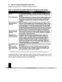
Table 1-1: Parameter and variable definitions of the general model settings
Initial year
.: "I
"
~
:.
,,:;'~~!t~:~;~~~~i\~'~;:~,.~"
..
.",,0.,:'
' .."!•..,•• "".~.i*;i!(~"s.
;.
<:
.'
:~ .. ~: .:~. .;~~:?~:'~~~;~ :.~
Land degradation impact
factor
The starting year of the projections. This is the year to which the baseline data apply.
Although this value could be changed, it is better not to do so as it corresponds to the
initial data.
The end of the projection period. All simulations will be run in single-year steps up to the
year specified here and all results will be stored up to the end of the specified period.
Although there is no direct limit set to the value of this parameter, projection periods
of longer than 50 years will slow down calculations and are subject to increasing
uncertainty.
Refers to the net daily per capita amount of food produced in the starting year. Food
production in PEDA is expressed in terms of its energy equivalent or calories. Note that
one has to specify this 'net' food production, that is the total production after deduction
of post-harvest losses and a fraction of the production reserved to be used as seeds in
the next cropping season. From this information and the level of post-harvest losses in
the initial year, PEDA automatically estimates the gross food production. Once the gross
production is determined for the initial year, PEDA projects it into subsequent years of
the projection period in single-year steps using the agricultural production function.
Refers to the net daily per capita Kcal imports in the starting year. Combined with the
net food production, it results in the net food available for consumption. Fluctuations in
net food imports during the projection period can be accounted for by manipulating the
scenario variable 'food imports and exports'.
In the PEDA model, calorie (energy) requirements are used as a proxy for food
requirements. "The minimum energy requirement is the amount of energy that is
required on average in a population to satisfy the basic physiological needs and
the needs for light activities of adults and the normal energy needs of children and
adolescents (inclUding the extra needs for growth). Two main factors determine
estimation of the energy requirement of a population, namely, the distribution by age
and sex and the body weight.-" The value of this variable, therefore, varies under
different national conditions, or the user can set the value to define different thresholds
in order to evaluate its effect on the model interactions.
This variable reflects the assumed negative impact of population growth on the natural
resource stock.
Proportion of cohort
(group of people born in
the same year) moving to
cities
This variable enables the user to set net rural-urban migration rates. A value of 0.2
means that of every cohort born in rural areas. 20% will move permanently to urban
areas over their lifetime. These movements are distributed over the different ages
according to standard age-specific migration schedules.
End of projection period
Net food production in the
initial year (in daily per
capita Kcal)
Net food imports in the
initial year (in daily per
capita Kcal)
Assumed minimum
consumption in Kcal per
capita to be food secure
This definition is taken from the African Nutrition Database Initiative (ANDI) website, at http://www.africanutrition.net/
In addition, the model uses a number ofpopulation variables including total fertility rate (TFR» lifeexpectancy
at birth. education (literacy rates). Unlike genera! setting parameters that are considered constant over the
projection period, the population variables are treated dynamically.
e,
•••
ZI:
--'II
Al
.1
un. _
A
1
B.
Dynamic parameter settings
Other input variables can be set in 'dynamic parameter settings'. They include variables of the agricultural
production function, variables influencing food availability at country level and HIV/AIDS (see table 2.2).
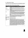
Table 2-2: Input variables in <dynamic parameter settings'
~ ~~~''1
•
.....
~.
. ~ ~'. ~J~~~,~'.:~'l~~t~~:·~·.~~:t~~
Fertilizer
Machinery
Technical education
Water
Irrigation
Size of the rural labour
force
Literacy of the labour
force
Land
Loss in transport and
storage
~~.~:~.:.~
z:; ·:;'4~'~A·:>~·1·~'.
"-.
:"
'~~~~;'~:.~''';'{~~-:':'
:' ~
;~.i,:.~A~·~;~:t~1"~~i· :·.<~·:-~.~J~·~:"i~~~';'
The amount and productivity of fertilizer used in agriculture. The user needs to set a value
that expresses a relative improvement/worsening with respect to the conditions in the
starting year.
The amount and productivity of machinery used in agriculture. The user needs to set a
value that expresses a relative improvement/Worsening with respect to the conditions in the
starting year.
In addition to literacy, the user can specify the technical capacity of the rural labour force
for agricultural purposes. As with fertilizer and machinery use, one needs to give a value
that expresses a relative improvementJ worsening of the conditions in a particular year as
compared to the starting year.
This covers the change in weather/climate conditions. Its initial value depends on the
climate conditions of the country at the time of initialization. The range of acceptable values
for the water scenario variable depends very much on the definition of the water saturation
curve. In the current version of PEDA, values for the water scenario variable can range
from 0 to 1.5, with 1 describing a situation of optimal rainfall conditions for agriculture.
Values higher than 1 indicate a surplus of water and have a negative impact on agricultural
outputs.
This covers the efforts made in irrigation, including pipelines, pumps, energy etc. The value
of this scenario variable expresses a relative improvement/worsening of the conditions in a
particular year as compared to the conditions in the year of initialization.
Endogenously determined variable.
Endogenously determined variable.
Endogenously determined variable.
Individuals will not consume all the food that is produced. Some of the food will be lost
during harvest, transport, storage or processing, and some of it will be used as seeds for
the next cropping season. For the initial year, one has to specify the proportion of gross
production that is not available for consumption for one of the reasons specified above.
For the subsequent years in the projection, the user can assume changes in post-harvest
losses by manipulating this variable. The range of possible values for this scenario variable
runs between 0 to 1, with 0 describing a situation where there are no post-harvest losses
and 1 a situation where none of the locally produced food is available for consumption.
Although one has to specify the net production in the initial year as part of the initialization
process, PEDA automatically recalculates the gross production. The latter is the basis for
estimation of food production in the following years of the projection period and from which
the post-harvest losses are deducted. Note that post-harvest losses are only applied to
locally produced food and not to net imports.
Urban bias factor
Food imports and
exports (net trade)
HIV/AIDS morbidity
rates
This variable enables the user to allocate food disproportionally between urban and rural
areas. A value of 1.0 means that the food is distributed proportionally to the size of the
population living in urban and rural areas respectively (a state of 'no bias'). A value of 1.1
means that urban areas receive 10% more food than would be allocated under conditions
of equal access. The remaining share of the food is then attributed to rural areas. By giving
a value lower than 1, the user can assume a 'rural bias' in access to food.
This variable allows the user to take changes in food imports and exports into account.
During the initialization process, one has to specify an absolute value for net food imports.
The dynamic scenario variable food imports/exports has a default value of 1 reflecting the
conditions in the initial year. By manipulating the value of this scenario variable, the user
can make different assumptions regarding net imports/exports. A value of 2, for example,
means that the amount of food imported has doubled compared to the initial year.
In the HIVIAIDS scenario variable, the user is expected to set an HIV/AIDS related
morbidity pattern over time that is deti ned in terms of proportions of the young adult
population, aged 15-49. A value of 0.02 for this variable means that 2 per cent of the young
adult population is assumed to be sick due to an AIDS-related complaint. In any population,
this proportion tends to be lower than the HIV prevalence rate because the period of
morbidity tends to be shorter than the incubation period.
2.2. Output Variables
Output variables include the standard ones shown in table 2.3.
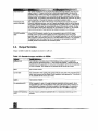
Table 2-3: Standard output variables in PEDA
;""., .
) ...
.
..,
.'
'
,.,
'."
~
;
, •• 0•
"
.
Awlable food
This is the sum of the total amount of food produced in the country in a particular
year minus the post-harvest losses, +/- food imports and exports. It stands for the net
available food to the population for each year in the projection period and it is expressed
in terms of calories. This indicator is only available for the country as a whole.
Births
Total number of births
Current land
The combination of the quantity and quality of land for each year of the projection period.
Index value summarizing the effects of land degradation and regeneration. This indicator
is only available for the country as a whole.
Dj9aths
Total number of deaths
Ufe expectancy (eO)
When requested for each of the eight subgroups separately and sex specific, this is
the graduated value of the assumptions of the user. At the country level, however, it is
also influenced by changes in the relative weights of the subgroups in the population
(provided that different life expectancies have been set for the different subgroups).
Literate Life Expectancy
(LLE)
Number of years a person is expected to live in a literate status from the age of 15
onwards.
~I
I
I
I
""
...I
I
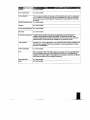
Fertilizer
Is an input variable.
Food import/exports
Is an input variable.
Food production
HIV/AIDS morbidity rates
This is the gross production for each year of the projection period, and it is expressed in
terms of calories. This indicator is similar to food availability, but it does not account for
post-harvest losses and imports/exports. This indicator is only available for the country
as a whole.
Is an input variable.
Irrigation
Is an input variable.
Loss in transport/storage
Is an input variable.
Machinery
Is an input variable.
Proportion food insecure
In addition to the population size that can be generated by urban/rural place of
residence, literacy status and food-security status; the model has an extra output
variable that portrays the proportion of food insecure in the country for any year of the
projection period. This indicator is only available for the country as a whole.
i Total population
Population size. It can be generated for each of the eight sub-populations separately and
for both sexes separately. There is also a possibility to extract age-specific information
directly from the databases.
Technical education
Is an input variable.
TFR
When requested for each of the eight subgroups separately, this is the graduated value
of the assumptions of the user. At the country level, however, it is also influenced by
changes in the relative weights of the subgroups in the population (provided that different
fertility rates have been set for the different subgroups)
... - - - - - - - : c - : - - - - - - = - - - - - - - - - + - : - - - - : - - - - c - - : - - : - - - - - - - - - - - - - - - - - - - - - - - - - - - - - j
Urban bias factor
Water
Is an input variable.
Is an input variable.
3.
How to Use the PEDA Software
3.1.
Generallnstructions
The PEDA software runs under Wmdows, is based on Excel spreadsheets and uses the Access database.
PEDA will run on any machine with Windows, but the power of the machine will influence the speed of
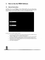
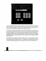
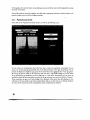
calculation. When you start the PEDA application, you will see the following welcome screen.
On this screen you can choose among four options:
•
•
•
•
"Learn about the model" will give you more information about the structure ofPEDA. The most
complete description is given in the Technical Manual (chapter 2).
"Simulation" will first ask you to choose from the drop-down list one of the countries that has
been initialized for PEDA and will then bring you to the country-specific simulation screen.
"Presentation of results" will directly bring you to the results of previously calculated and stored
scenarios for the countries indicated.
"Exit" will end the application.
3.2. Using Scenario Settings and Simulations
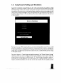
If you click on Simulation, e.g. for Ethiopia, you will see the country-specific screen, Welcome to PEDA
Ethiopia, that is shown below. PEDA can only be run for countries that have been initialized. This means that
data on the starting conditions and on certain country-specific settings have already been entered. Initializing
the model for a new country is not a trivial task and requires substantive analysis and knowledge about the
country as well as sufficient knowledge of Excel. More information about the initialization process is given in
the Technical Manual (chapter 5). Here we only discuss the scenario variables and parameters that can be set
on this user surface.
The button on the top "Read Scenario" allows you to load an already predefined scenario. This is a useful
option if you already have a certain baseline scenario for a chosen country that can serve as a starting point
to create another scenario by changing only a few variables. Other buttons let you save the current scenario
settings under a user-defined name and start the simulation (once you are satisfied with all parameter settings
for one specific scenario).
The next two buttons, i.e. "General settings and population parameters" and "Dynamic Parameter Settings"
enable you to define new scenario variables and parameters by changing the current scenario settings. The
setting of scenarios can be done in two different modes. The "General settings and population parameters"
button allows you to change parameters that are kept constant over the projection period or can be set to
change in a piecewise linear fashion over time (such as fertility and mortality). For other variables under the
"Dynamic Parameter Settings" button, you can freely define any time path over the simulation period. In
order to set those parameters or see what the predefined values of the parameters are, click the appropriate
box.
The last "Go to the Main Screen" button lets you go back
to
the main screen.
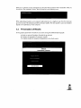
3.2.1. General model settings and population parameters
If you dick on the "General settings and population parameters" button you get the following screen:
If you choose the folder "General" tab, you will be able to set some of the basic model specifications that
cannot be changed over time or across sub-populations.
Among these general parameters you can first specify the initial year of your calculations. This is typically the
year for which the specific-country application has been initialized, i.e. in most cases, the last year for which
empirical information is available (but you can also choose other dates if you have specific reasons to do so,
such as simulating "alternative histories"). Next, you can determine the end of the projection period. All
simulations will be run in single-year steps up to that year and all results will be stored up to the end of the
specified period. PEDA will run scenarios for end points up to the year 2050.
JIIj
On this general parameter screen, you can also enter the net amount of food produced and imported expressed
in terms of kilocalorie available per capita per day in the initial year. You can also enter the assumed minimum
energy (in Kcal) required for each individual of the country in order to be considered food secure. This
minimum requirement can be chosen according to the definition of malnutrition and food security that you
prefer. It will enter the calculations for determining the proportion of the population that will be considered
food insecure. This specification will have significant impact on the results. If the minimum requirement is
specified rather high, this will result in a greater proportion of the population considered food insecure and
vice versa.
On this screen, you can also set the "Land degradation impact factor" which lets you define the assumed
impact of an increase in the food-insecure, rural, illiterate population on the land variable. This factor will
enter a non-linear land degradation function (see Technical Manual), which also considers population density
and the state of the land resource. The state ofcurrent land (which combines quantity and quality aspects) will
then enter the food production function. This assumed effect of an increase in the food-insecure rural illiterate
population is one of the two feedback loops in the model that go from the population to food production. The
other one operates through the size and skill level of the population.
Since this model distinguishes between urban and rural areas, migration between the two areas also needs to
be considered. This is done by making assumptions on the net movements from rural to urban areas, which
is specified here in terms of the proportion of a cohort moving to cities. A value of 0.2 means that of every
cohort (that is, group of people born in the same year) 20% will move permanently to urban areas over
their lifetime. In the actual calculations these movements are distributed over the different ages according to
standard age-specific migration schedules.
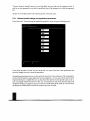
If you go to the tab "Sub-populations" you can set parameters separately for each of the eight sub-populations
listed. By cross-classifying food-security status, literacy status and rural/urban place of residence eight states
are being defined and PEDA performs population projections by age (single year) and sex for each of the
groups, also considering movements between the groups in every year. By simply clicking on the field with the
name of the sub-population, e.g. the rural/ illiterate/food secure as seen on the screen below, you get a form
for defining trends in fertility and mortality of that specific sub-population and educational transition rates
for women and men.
For setting future trends fertility, as described by (he Total Fertility Rate (TFR), i.e. the mean number of
children per woman, and mortality, as described by life expectancy at birth follow a similar scheme. The user
has to first enter the values for the starting year of the simulation
(a question of getting empirical data or appropriate estimates). Then, scenario assumptions for fertility and
female and male life expectancy for three points in the future can be entered. If two subsequently specified
values are different, the model will automatically calculate a gradual linear change between the two points in
time. Hence, the specified fertility and mortality scenarios will be piecewise linear.
The user has to keep in mind that the resulting trend in the fertility and mortality of the total population does
not only follow from the paths specified in this manner but will also be influenced by the changing weights
of the various sub-populations. Ifyou assume, for instance, constant fertility at 4.0 for the illiterate and at 2.0
for the literate population, and over time the female population of reproductive age will become more literate,
the aggregate fertility level of the. total population will show a declining trend. In this sense, the aggregate
fertility and mortality levels are already a result of the scenario calculation and cannot be specified as a specific
scenario assumption.
Under "Education" you can specify the proportion of women and men in each birth cohort that will move
over their lifetime from the illiterate to the literate state. The age pattern of this transition to the literate state
can be specified during the initialization process. For sub-groups that are already educated you will see a
screen without educational transition because, in PEDA, there is no movement hack to the illiterate state.
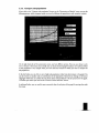
3.2.2. Dynamic parameter settings
If on the country-specific screen ("Welcome to PEDA Ethiopia") you choose the button with "Dynamic
parameters setting" you will see the following screen. You can choose from the right hand list (which you get
by clicking on the little arrow next to the currently listed variable) which scenario variable you want to set.
The exact interpretation of these variables and the functional form in which they enter the model are given
in the Technical Manual (chapter 3). Fertilizer, machinery and technical education will directly enter the
food production function with certain elasticities. "Food import/export" and the "Urban bias factor" relate
to the distribution of food to the population. Water is essentially a climate variable referring to rainfall and
soil moisture. The initial value of water is set during initialization to correspond with the country's climate
conditions. The impact of water on food production is modeled in a highly non-linear way. with additional
water having a strong effect under dry conditions, then coming to saturation where more water brings little
change in output and finally moving to flood conditions where more water is destructive. Decreasing or
strongly increasing the water variable in certain periods can simulate droughts or floods. The irrigation variable
measures the efforts in irrigation but its effect will also depend on the availability of water.
''AIDS morbidity" givesan estimate ofthe proportion ofthe young adult population that is already symptomatic
with AIDS. This specified level will influence the shape of the age-specific mortality curves applied. Its setting
should be consistent with the time paths assumed for life expectancy. The Technical Manual gives information
on how [0 do this (chapter 5).
Except for AIDS morbidity and water, these variables are all treated in index form, which means that their
level in the starting year is set to be 1:0 and their levels in all the subsequent years are seen as relative to this
starting year. This setting allows you to use the model even if you do not have empirical information about
the exact quantitative level of each factor since you only have to specify the relative change as compared to
the starting year.
You can change the factors over time either by setting the values numerically in the table below the chart (click
on "Change values in table" in upper-right corner) or by applying a constant rate of annual growth (click on
"Annual growth").
For practical reasons, the options for setting values numerically are limited here to every fifth year with
intermediate years being interpolated for the simulations.
It is also possible (0 combine the automatic application of a growth rate with specific numerically entered
deviations from the exponential path in certain periods. For this you must first apply a constant growth rate
(do nor forget (0 apply it by clicking the OK button), then switch to the manual setting option and change
the values in the table as desired. The graph will always give you a representation of all annual values resulting
from that procedure.
3.2.3. Simulation
After you have set all the scenario parameters, you click the "Return" button and go back to the countryspecific welcome page. There you save the new scenario that you have just defined by clicking the "Save
scenario" button. Saving the new scenario assumptions under a new scenario name is the pre-requisite for
simulation. "When saving, you may specify in the "Short description" box more detailed information about
what you have assumed in the scenario, for future reference. After saving has been done, you need to read the
same scenario by clicking the "Read scenario" button and selecting the scenario you have created. This action
allows you to upload all scenario assumptions into the place where simulation will be undertaken. Then you
can click the "Start simulation" button. This will bring you to the following screen:
Simulation in progress
While undertaking simulation. your computer makes projections in a single-year step from the initial year
up to the last year of the projection period for all output variables. The time required to carry out simulation
depends on the performance of your computer.
3.3.
Presentation of Results
For the graphical presentation of results you can choose among three different kinds of graphs:
(a) Simple or animated Population Pyramids (by age and sex);
(b) Compare sub-populations for any given scenario;
(c) Compare scenarios for any given sub-population or the whole country.
On the graphs, the numerical values corresponding to any point of the line charts will be displayed by moving
the mouse to that point.
Since all the results are stored in a database, any table with an appropriate selection of numerical data can be
printed on paper or put in a file for further processing.
3.3.1. Population pyramids
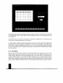
If you click on the "Population Pyramids" button, you will see the following screen:
For any scenario or sub-population (here called state due to multi-state population terminology) that you
choose, you see the usual age pyramid with men on the left and women on the right, sorted by age. For the
purpose of display, the single-year age groups of the model have been aggregated into 5-year age groups.
By moving the time bar (click on the centre piece and move left or right while holding it), you can choose
an age pyramid for any simulation year (in a single step or 5-year steps). Alternatively, you can choose an
animation, which will show the gradual evolution of the age structure over time if you dick on "Animate",
These animations can give you a better feeling of the dynamics of the system than only looking at static
information. The year stated on top of the pyramid always tells you at what year you are looking. Similarly,
the names of the scenario and of the sub-population under consideration are indicated.
.R.lI
•
\!It.:.
IQ
•
v ...
oM
I'
L
t
_It
j
JIJL,'.I'-M@--
. b'!J.t4
"" r,
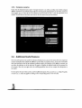
3.3.2. Compare sub-populations
If you click on the "Compare sub-populations" button on the "Presentation of Results" screen, you get the
following picture, which compares trends over time for different sub-populations under one given scenario.
On the right hand side of this presentation screen, you have different options. First. you can choose to plot
men or women or both sexes and, secondly, you can choose the demographic indicator to be plotted, which
is total population in our example. Next, you must select the scenario for which you want to compare the
sub-populations.
In the box below, you can click on any of eight sub-populations (called state here) shown in the graph. You
can also choose any number and any combination of sub-populations. Moreover, by clicking on the button
"Aggregate"below you can calculate the sum of the chosen sub-populations to be also presented on the graph.
To confirm your choice you must hit the "Click to Confirm Selection" button.
As indicated before, you can read the exact numerical value of each point of the graph by moving there with
the mouse.
3.3.3. Compare scenarios
If you click the third presentation option "Compare Scenarios", you will see a similar screen, which compares
different scenarios for any selected output indicator and any specific sub-population or the whole country; To
do this again, you can choose the sex, the indicator to be plotted and the state (i.e. the sub-population) to be
studied. You will then see line charts over time for all the scenarios that you have defined.
3.4. Additional Useful Features
One very useful option is that under the selection of indicators you can also view some of the most important
scenario assumptions that underlie the different scenarios that you examine. Hence, if you do not remember
what you assumed in terms of the machinery production factor, for example, in the different scenarios, you
can select this indicator on the list and then the graph will display the assumed trends of this parameter for
all scenarios. After this, you again select the resulting population size and can compare the assumptions to
the results.
On the top line of each of these screens, you find additional options. You can zoom in, i.e. enlarge the graph,
or zoom out, i.e. reduce the graph by clicking on the corresponding boxes on (he menu bar.
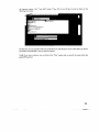
An important option is the " Save table" button. If you click it, you will get an insert as shown on the
following screen print:
On this insert, you can specify the file name under which the table should be scored. These tables can then be
formatted and transformed in any way that Excel allows.
Finally. if you wane a printout, you can click on [he "Print" options and can specify the printer where the
graph will be printed.
19
._--_
....
>.~~...,
.... , •• -