Download Infrared Sensors for Counting, Classifying, and

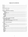
Technical Report Documentotion Page
1. Report No.
2.
Government AcceSSion No.
3.
Rec,p,ent's Cataiog No.
FHWA/TX-9l+ll62-1F
4.
Title and Sub."le
S. Repor.Do'e
December 1990
INFRARED SENSORS FOR COUNTING,
CLASSIFYING, AND WEIGHING VEHICLES
6.
r - - : ; - - - - ; - - - ; - - ; - - - - - - - : - - - - - - - - - - - - - - - - - - - - - - - - - f 8.
Joseph E. Garner,
Clyde E. Lee, and Liren Huang
7.
Autharls)
Performing Organization Code
P erformi ng
0 rganl
zatl on Report No.
Research Report l162-1F
9. Performing Organization Name and Address
10. Work Unit No. (TRAIS)
I
Center for Transportation Research
The University of Texas at Austin
Austin, Texas
78712-1075
11. Contract or Grant No.
Research Study 3-10-88/0-1162
~~~----------------------------------------------------~
13.
12. Sponsoring Agency Name and Address
Texas State Department of Highways and Public
Transportation; Transportation Planning Division
P. o. Box 5051
Austin, Texas
78763-5051
1S.
Type of Report and Pettad Covered
Final
14. Sponsoring Agency Code
Supplementary Nates
Study conducted in cooperation with the U. S. Department of Transportation, Federal
Highway Administration. Research Study Title: '~nfrared Detectors for
Counting, Classifying, and Weighing Vehicles"
16. Abstract
In this study, five field tests were conducted to determine the feasibility of
using commercially-available infrared light-beam sensors for counting, classifying,
and perhaps weighing vehicles. It was demonstrated that a Single, reflex-type
infrared sensor mounted just off the shoulder and working off a retro-reflective
raised pavement marker in the center of the outside traffic lane can be used to
count the tires on one end of each axle of a moving vehicle with accuracy comparable to human observers or to a flush-mounted piezo-strip sensor. Sensor installation involved no pavement cuts and only minimal interference to traffic. Tests
were not conducted in snow or heavy rain. Arrays of two or more infrared lightbeam sensors can be used to sense vehicle-body presence, to calculate vehicle
speed, axle spacing, and tire-contact patch dimensions, to indicate single or dual
tires, to detect direction of vehicle movement, and to sense over-height vehicles.
Off-shoulder reflex-type infrared sensors with retro-reflective raised pavement
markers operated for up to three months without cleaning. A two-sensor array
tested in the Houston high-occupancy-vehicle (HOV) lane indicated promise as a
replacement for loop-detector arrays. Infrared sensors can supplement weigh-inmotion systems by indicating off-transducer vehicle tires, but correlations between
infrared light-beam sensor measurements and weight were not sufficient to make
adequate weight estimates from such measurements practicable.
18. Distribution Statement
17. Key Words
infrared light-beam sensors, retroreflective, pavement, vehicles, speed,
axle spacing, weight, arrays, traffic,
weigh-in-motion systems, estimate
No restrictions. This document is
available to the public through the
National Technical Information Service,
Springfield, Virginia 22161.
19. Security Classil. (of this report)
20. Security Classi f. (of thi s page)
Unclassified
Unclassified
Form DOT F 1700.7
(8-72)
Reproduction of completed page authorized
21. No. of Pages
80
22. P ri ce
INFRARED SENSORS FOR COUNTING,
CLASSIFYING, AND WEIGHING VEHICLES
by
Joseph E. Gamer
Clyde E. Lee
Liren Huang
Research Report Number 1162-1F
Research Project 3-10-88/0-1162
Infrared Detectors for Counting, Classifying, and Weighing Vehicles
conducted for
Texas State Department of Highways
and Public Transportation
in cooperation with the
u.S. Department of Transportation
Federal Highway Administration
by the
CENTER FOR TRANSPORTATION RESEARCH
Bureau of Engineering Research
THE UNIVERSITY OF TEXAS AT AUSTIN
December 1990
The contents of this report reflect the views of the
authors, who are responsible for the facts and the accuracy
of the data presented herein. The conten ts do not necessarily
reflect the official views or policies of the Federal Highway
Administration or the State Department of Highways and
Public Transportation. This report does not constitute a standard, specification, or regulation.
There was no invention or discovery conceived or fIrst
actually reduced to practice in the course of or under this
contract, including any art, method, process, machine,
manufacture, design or composition of matter, or any new
and useful improvement thereof, or any variety of plant
which is or may be patentable under the patent laws of the
United States of America or any foreign country.
ii
PREFACE
Throughout this research study, a number of agencies, companies, and individuals cooperated in providing
infonnation, helpful suggestions, materials, personnel,
and other resources to support the work. The study contact individuals representing, respectively, the State Department of Highways and Public Transportation and the
Federal Highway Administration were Jeff Seiler and Ted
Miller. Their timely contributions of administrative and
engineering support made the research possible. Personnel in D-IO, Transportation Planning Division, cooperated generously in all phases of the effort, especially in
scheduling and conducting the field studies at Seguin,
Junction, San Marcos, and Jarrell, and by loaning hardware. Similarly, D-9, Materials and Tests Division, furnished sample retroreflectors and epoxy. Posts and retroreflectors were furnished by District 14, Austin.
Department of Public Safety officers cooperated in the
field measurements of tire-contact dimensions and weighing of trucks at San Marcos. The sensor tests in the highoccupancy-vehicle (HOV) lane in Houston were made
possible by the efforts of Dick McCasland and Gene
Ritch with the Texas Transportation Institute, and those
of Lynn McLean and his associates with Houston Metro.
Chet Freda, representing Motorola Inc. 's University Support Program in Austin, furnished, at no cost, numerous
microprocessor devices and electronic components and
also supported the research through Motorola's facilities
in Phoenix. Southwestern Materials provided retroreflectors of various types for experimentation. All these contributions, and others not mentioned specifically, are sincerely appreciated.
ABSTRACT
In this study, five field tests were conducted to
detennine the feasibility of using commercially-available
infrared-light-beam sensors for counting, classifying, and
perhaps weighing vehicles. It was demonstrated that a
single, reflex-type infrared sensor, mounted just off the
shoulder and working off a retroreflective raised
pavement marker in the center of the outside traffic lane,
can be used to count the tires on one end of each axle of
a moving vehicle with accuracy comparable to that of
human observers or that of a flush-mounted piezo-strip
sensor. Sensor installation involved no pavement cuts
and only minimal interference to traffic. Tests were not
conducted in snow or heavy rain. Arrays of two or more
infrared-light-beam sensors can be used to sense vehicle-
body presence; to calculate vehicle speed, axle spacing,
and tire-contact patch dimensions; to indicate single or
dual tires; to detect direction of vehicle movement; and to
sense over-height vehicles. Off-shoulder, reflex-type
infrared sensors, with retroreflective raised pavement
markers, operated for up to three months without
cleaning. A two-sensor array tested in the Houston highoccupancy-vehicle (HOV) lane indicated promise as a
replacement for loop-detector arrays. Infrared sensors
can supplement weigh-in-motion systems by indicating
off-transducer vehicle tires, but correlations between
infrared-light-beam-sensor measurements and weight
were not sufficient to make adequate weight estimates
from such measurements practicable.
iii
SUMMARY
Infrared sensors can be used in three sensing modes:
direct, reflex, or diffuse. The reflex mode, which requires a retroreflector, can be used in all applications discussed in this report. For a few applications such as vehicle-height detection, the direct-sensing mode, which
requires the transmitter and receiver to be in separate locations, can also be used. The diffuse-sensing mode is
not recommended for traffic applications.
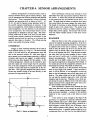
Overhead, roadside, and pavement level are the three
different arrangements of infrared sensors which can be
used. In the overhead and roadside arrangements, vehicle
bodies are sensed, and vehicle speed, length, and
headway can be calculated. In the pavement-level
arrangement, tires are sensed, and speed, axle spacing,
tire-contact-patch dimensions, and lateral position of tires
can be calculated. Also with this sensor arrangement,
single and dual tires can be identified.
In the ftrst two fteld studies, it was determined that
the in-motion tire-contact patch constantly changes and is
sometimes considerably different after the vehicle travels
only a few inches. Attempts were made to correlate the
in-motion dimensions of tire-contact patches with wheel
weights of 149 semi-trailer trucks which were measured
simultaneously with weigh-in-motion force transducers.
Only a rough correlation was found for the dual tires on
tandem axles, and virtually no correlation was found for
the single tires of the front axles. These correlations between infrared-light-beam-sensor measurements and
weight were not judged to be sufficient to make adequate
weight estimates practicable. WIM system measurements can be aided by using infrared-light-beam sensors
to make lateral-position calculations which identify offtransducer tires.
In a field test in a high-occupancy-vehicle (HOy)
lane in Houston, an array of two infrared sensors was the
basis for calculating vehicle speed, length, and headway,
and for indicating direction. The current array of three
loop detectors can possibly be replaced with infraredlight-beam sensors after only minor modiftcations of the
infrared-sensor housing and the currently-implemented
computer software.
In an extended performance test, it was determined
that off-shoulder infrared sensors and in-lane retroreflectors can be operated for three months or longer without
cleaning or adjustment. These tests were conducted in
the summer and fall months in Texas.
In another fteld test, an array of two pavement-level
infrared sensors was used to count axles per vehicle and
indicate single and dual tires as the basis for classiftcation. The two-sensor infrared array, combined with a
loop detector, had a 95 percent success rate during periodic evaluation over a thirty-day period at a site where
vehicles were traveling between about 50 and 65 miles
per hour. Experienced human observers were the basis
for the accuracy comparison.
IV
IMPLEMENTATION STATEMENT
Arrays of infrared sensors and retra-reflectors in both
the overhead and roadside arrangements can indicate
vehicle presence and direction and thus provide
information for counting vehicle bodies and for
calculating vehicle speed, headway, and length. In the
overhead arrangement, vehicles can be counted by lane.
In the roadside arrangement, the height of vehicles can be
determined. Arrays of infrared sensors and retroreflectors
can be used in the pavement-level arrangement to
calculate axle speed, axle spacing, tire-contact-area
dimension, and lateral position of tires. They can also be
used to indicate single or dual tires. Another sensor,
either an infrared sensor placed to detect vehicle bodies
or an inductance-loop detector, is required to match tires
to the correct vehicle for classification. For longer-term
performance, off-shoulder mounting of the reflex-type
infrared sensors with retroreflective raised pavement
markers in the center of the outside lane is recommended.
Sensors on the edge line work only a few days without
cleaning of the lenses and retroreflectors. Some infrared
sensors are battery-powered and have a built-in counter
with LCD display. These units cost about $130 each and
are recommended for non-recording counter applications,
perhaps at remote locations, where total counts can be
recorded by a human observer at appropriate intervals.
Output signals from infrared sensors can be connected to
a counter or classifier which normally accepts road-tube,
loop-<ietector, or piezo-cable input signals. These output
signals can also be processed by a software program
stored on a single-chip microprocessor board. Data can
be stored on the board or sent to a computer to be
displayed and stored. In-motion tire-<:ontact dimensions
measured with infrared-light-beam sensors were not
found in this study to be an adequate basis for estimating
vehicle weight and tire loads of static vehicles and are,
therefore, not suggested for implementation. The
reliability of weigh-in-motion measurements can be
enhanced with infrared-sensor information which detects
off-transducer positions of the tires of vehicles being
weighed. The cost of an infrared reflex sensor and
reflector is about $100, while a piezoelectric cable costs
over $300 and requires traffic control and pavement
cutting to install it.
v
TABLE OF CONTENTS
PREFACE ..................................................................................................................................................................................................................... iii
ABSTRACT ................................................................................................................................................................................................................. iii
SU"MMARy..................................................................................................................................................................................................................
IV
Th1PLEMENTAnON STATEMENT.................................................................................................................................................................
V
CHAP1ER 1. INIRODUCIlON..................................................................................._................................................................................. ..
CHAP1ER2. PHOTOELECTIUCFUNDANrnNTALS
Developn1elll................................................................................................................ _.................................................................................... 2
Electric Eyes..............................................................................................................................................................................................
Light-Emitting Diodes ...........................................................................................................................................................................
Sensing Modes...................................................................................................................................................................................................
Effective Beanl..................................................................................................................................................................................................
Excess Gain.........................................................................................................................................................................................................
Contrast........................................................................................................................................................................................................
Retroreflecta'S....................................................................... __ ............_....... __ ............ _..........................._.............. _...... _..._........................
Summary......_..............................................._................. _._... _..... _....... _..............._ .... _._ ... _..._..............................._.....................................
2
3
CHAP1ER 3. VEIDCLE CLASSIFICATION SCHEMES
Federal Highway Administration ................_............_.... _......_....__......................._. __ .._.....................................................................
Oklahoma Turnpike Authority ........................ _.... _............_............._... _.. _............................................................... _.............................
American Association of State Highway and Transportation Officials..................................................................................
American Society for Testing and Materials ................................................. _...................................................................................
5
5
5
6
2
2
3
3
3
3
Summary.................................................................................................._........................................................................................................... 6
CHAP1ER 4. SENSOR ARRANGEMENTS
()verhead...............................................................................................................................................................................................................
7
Roadside ._ ................................................................................................................................_.......................................................................... 7
Pavement-Level .............................................._.............. _ ... _..............._................_................................................................_..................... 8
Summary............................ _.................................................................................................._..........................._.............._................................ 9
CHAP1ER 5. APPLICATIONS
Vehicle Presence..............................................................................................................................................................................................
Counting........................................................... _........... _.... _............................ _....... _.......... _............._..............................................................
Direction ...................................................................._....... _................................._. __..........._..........................................._.............................
Vehicle Height.................................................. __ ................................__ ... ___ ........ _..... _.................................... _......_................................
Speed........_..._....................................................._.....__..................................._..............................._.................................................................
C1assifialtion............................................................................................................... _........................._..........................................................
Weighing ...................................................................._._......._................._._ ......... _..... _.._._................................_.........._...............................
10
10
10
10
10
10
10
Summary..............................................................................................................................................................._.............................................. 11
vi
CHAPTER 6. FIELD EV ALUATIONS
Equipment and Software ...............................................................................................................................................................................
Tire-Contact Area............................................................................................................................................................................................
Weight ...................................................................................................................................................................................................................
Speed, Axle Spacing, and Lateral Position ................................................................................................................................
Front Axle ...................................................................................................................................................................................................
Tandem Axles ...........................................................................................................................................................................................
All Axles......................................................................................................................................................................................................
12
12
13
13
14
15
18
SUI1UTI3I'Y................................................................................................................................................................................••• ..... .••• .•••. .•... 19
HOV Lanes .......................................................................................................................................................................................................... 19
Endurnnce. ............................................................................................................................................................................................................ 20
Single/Dual Tire Identification and Vehicle Classification......................................................................................................... 21
SUI1UTI3I'Y•••••••••••••••••••••••••••••••••••••••••••••••••••••••••••••••••••••••••••••••••••••••••••••••••••••••••••••••••••••••••••••••••••••••••••••••••••••••••••••••••••••••••••••••••••••••••••••••.. .............. 21
CHAPTER 7. CONCLUSIONS .......................................................................................................................................................................... 23
REFEREN"CES ............................................................................................................................................................................................................ 24
APPENDIX ................................................................................................................................................................................................................... 25
vii
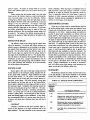
CHAPTER 1. INTRODUCTION
Transportation engineers require infonnation about
traffic and traffic loadings in order to design pavements
and other structures that will endure and function adequately throughout their design life. Pneumatic road
tubes. piezoelectric cables. and inductance-loop detectors
are some of the sensing devices commonly used to count
and classify traffic. Weighing is done both statically and
dynamically. Static weighing uses special scales to measure the tire forces of a standing vehicle. Static vehicle
weights can also be closely approximated by measuring
the dynamic tire forces of a moving vehicle with weighin-motion transducers and by processing the force signals
with electronic instruments. Most of the sensors currently in use for counting. classifying. and weighing
moving vehicles require mounting in the pavement or on
the pavement surface in the traveled lane.
The purpose of the research described herein was to
detennine the feasibility of using commercially-available
infrared-tight-beam sensors for some. or all. of these purposes. A primary objective was to sense the presence of
a vehicle or a tire traveling in a highway lane without
cutting into the pavement surface or having hardware on
the surface where it would be impacted by the tires of every vehicle. It was felt that commercially-available infrared sensors have potential for use in counting. classifying, and weighing vehicles. The considerations in
selecting candidate photoelectric sensors. designing the
needed hardware and software. installing the systems at
selected field sites. and evaluating their perfonnance. are
presented in this report.
The tests of infrared sensors for counting and
classifying vehicles described herein began in 1988. In a
test near San Marcos. Texas. in-motion infrared-sensor
measurements of tire-contact area and axle spacing were
compared with manual measurements taken after the
vehicles were stopped by Department of Public Safety
personnel. In another test near Seguin. Texas. infrared
and WIM measurements were taken concurrently and
compared. Overhead mounting was tried in a series of
tests in Austin. In 1989. a test was perfonned on a highoccupancy-vehicle (HOV) lane in Houston to detennine
the feasibility of a two-sensor system to calculate speed.
headway. length. and direction and to possibly replace
loop detectors at locations where pavement cuts were not
feasible. A test similar to the one at Seguin was
performed at Junction. Texas. with improved infrared
equipment. In 1990 a test was made near Jarrell. Texas,
to determine long-term performance and durability.
Comparisons were also made of vehicle classification
systems using loop detectors and a piezo-cable sensor.
Another test was made on the Turner Turnpike in
Oklahoma City to determine the possibility of using
infrared sensors for auditing toll collection based upon
eight vehicle classes. Other tests were performed on
several streets in Austin.
A self-contained data-collection and storage unit to
be mounted on the pavement surface at the lane line was
designed and constructed. but field testing was considered unwarranted after observing disabling amounts of
road ftlm accumulating on sensor lenses and retroreflectors after only two or three days of traffic.
This report will first describe how infrared sensors
operate. Next, it will list a few of the vehicle classification schemes currently in use. It will then discuss different ways in which sensors and retroreflectors can be arranged. Finally. it will discuss various applications and
field experiments using infrared sensors.
1
CHAPTER 2. PHOTOELECTRIC FUNDAMENTALS
A basic knowledge of photoelectric fundamentals is
essential to understanding the arrangements, applications,
and limitations of infrared sensors as they are used to
count and classify vehicles in motion. This chapter gives
a brief history of photoelectric sensors and introduces
concepts and terminology.
In some applications, LEOs operating in the less efficient,
visible-light wavelengths are preferred for ease of alignment
SENSING MODES
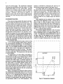
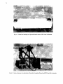
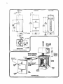
As shown in Fig 2.1, photoelectric sensors are used
in three main types of sensing modes or configurations,
each having distinct properties and applications. The flIst
sensing mode is called direct, opposed. or through-beam.
The source and detector are in separate, opposing
locations and the object to be sensed passes between
them and breaks the light beam. The second mode.
called retroreflective or reflex, has the source and
detector side-by-side, usually in the same housing. A
retroreflector receives the beam from the source and
reflects it back to the detector. The object to be sensed
passes between the source-detector and the retroreflector.
The third mode, called diffuse or proximity, has the
source and detector side-by-side with both aimed at a
DEVELOPMENT
ELECTRIC EYES
Photoelectric sensors have been around since the
1950's when incandescent lamps were used with cadmium sulfide photocells in systems commonly called
electric eyes. When sufficient light hits the surface of the
photocell, it conducts current to an output device. When
the light is blocked, the cell stops conducting current and
the output device directs an electric circuit to open a door
or perform some other action. Several drawbacks of this
system are that the incandescent bulb burns out rather
quickly and is susceptible to vibration and temperature;
both the bulb and the photocell are covered by lenses
which must be carefully focused; and the photocell can
be activated by other light sources such as the sun. Beginning in the 1940's, un modulated visible light beams
were used for traffic sensing, but with only limited success.
001(
1---__
Saulte
Receiver
1 . . . . -_ _ _
)
UGHT·EMIITING DIODES
Light-emitting diodes (LEOs) were developed in the
1960's and became available in the 1970's. They are
now widely used in calculator displays, watches, and optical sensors. LEOs are semiconductors made from materials such as gallium arsenide which emit light in a single
wavelength when current flows through them in the forward direction. They have life spans much longer than
those of incandescent bulbs and are not sensitive to
shock, vibration, or extreme temperatures. LEDs are
much smaller, which makes it possible for the packaging
to be more rugged and weather-resistant
Probably the biggest advantage of LEOs is their ability to be modulated, or turned on and off, thousands of
times per second. Photodetectors tuned to this same
modulation frequency ignore all other light sources,
though the source may be thousands of times brighter.
This alleviates the problems of critical alignment, partial
blocking, and extraneous light.
LEDs operate in several visible-light wavelengths as
well as infrared. Infrared light has a wavelength greater
than about 800 nanometers (nm). Gallium arsenide LEOs
emit infrared light in a tight band around 940 nm. Infrared LEOs are often preferred because they emit more
light intensity than visible-light LEOs and because most
photodetectors are more sensitive in the infrared range.
Direct Sensing
Soulte
Retroreflector
Receiver
Opaque Object
Reflex Sensing
Soolte
Object with
Reflective Surface
Receiver
Diffuse Sensing
Fig 2.1. Sensing modes.
2
3
point in space. An object is sensed when it is at this
point and reflects light from the source back to the
detector.
Direct sensing has the longest range. since the light
beam travels the distance between source and detector
only once and energy is not lost by reflection. Reflex
sensing has a shorter range. since the light beam crosses
the distance between sensor and retroreflector twice and
energy is lost by reflection. An object with high
reflectivity might not be detected in the reflex mode if it
reflects sufficient light back to the detector. To alleviate
this effect. polarizing filters may be used to filter out
specular reflections. but the resulting sensing range will
be reduced. The range of the diffuse sensing mode depends on the amount of light reflected by the object to be
detected.
EFFECTIVE BEAM
The effective beam is the energy that an object must
block for detection. For direct and diffuse sensing. the
effective beam is detennined by the overlap of the radiation pattern from the source and the field of view of the
detector. For the reflex mode. the effective beam is defined by the edge rays traced from the sensor lenses to
the edges of the retroreflector (Ref 1). For reliable detection. the object to be detected must shadow the entire retroreflector at one time. Larger retroreflectors may be
used to increase the sensing range. but the effective beam
size is also increased and. therefore. so is the necessary
size of the object to be detected.
beam is blocked. When the beam is completely blocked,
light received is zero and contrast is infinite. Contrast
should be as high as possible for optimum reliability.
This is important when the light beam is partially
blocked. or when a specular reflection is returned to the
detector. Contrast can be controlled by adjusting the sensitivity. or excess gain. of the detector.
RETROREFLECTORS
There are two basic types of retroreflectors used for
the reflex-sensing mode: corner-cube and spherical-bead.
Corner-cube retroreflectors consist of tiny plastic prisms
embossed in thin films. Spherical-bead retroreflectors
consist of glass beads embedded in a diffuse reflecting
binder (Ref 3). Both types have the property of returning
incident light beams straight back to the source as long as
the angle of light incidence is less than about 15 degrees.
The corner-cube type is more efficient than the sphericalbead type. If a polarizing fIlter is used on the sensor. the
corner-cube retroreflector will reflect polarized light The
corner-cube type is commonly used on streets and highways in raised pavement markers and in guide signs.
Both types are also available as reflective sheeting. For
best efficiency. provision must be made to protect retroreflectors from accumulations of dust and moisture. This is
usually accomplished with a clear plastic or glass cover.
The size and efficiency of retroreflectors detennine the
excess gain as described above and also the sensing
range. Larger retroreflectors. or an array of retroreflectors. will reflect more light energy. thus increasing the
range. excess gain. and effective beam size.
EXCESS GAIN
Excess gain is the ratio of the light energy received
by the detector to the minimum energy required for detection under ideal conditions. Ideal conditions are clean
air and clean lenses; i.e .• the beam is not attenuated.
Each sensor has an excess gain curve which shows excess gain versus range. For reflex sensing. excess gain
also depends on the type and size of the retroreflector.
Excess gain is greatest at close range and falls to one at
the maximum range. Guidelines for choosing sensors on
the basis of excess gain are given in Table 2.1. The operating environment includes a cleaning schedule for
lenses. An excess gain of 1.5X for a clean environment
includes a safety factor. An excess gain of SOX will penetrate see-through paper or thin cardboard. In this study.
the environmental effects of concern were dust, dirt. oil.
moisture. and shock and vibration from cars and heavy
trucks.
CONTRAST
Contrast is defined as the ratio between light received by the detector in the light condition and in the
dark condition. The dark condition occurs when the light
SUMMARY
Photoelectric sensors have been used for many years.
In the past decade. it has become feasible to use infrared
sensors for traffic engineering applications. The three
TABLE 2.1. EXCESS GAIN GUIDELINES
Source: Ref 2
Minimum
Excess
Gain
Required
l.SX
SX
Operating Environment
Clean air: no dirt build-up on lenses or reflectors
Slightly dirty: slight build-up of dust, dirt, oil.
moisture, etc. on lenses or reflectors; lenses
are cleaned on a regular schedule
lOX
Moderately dirty: obvious contamination of
lenses or reflectors, but not obscured; lenses
cleaned occasionally or when necessary
SOX
Very dirty: heavy contamination of lenses; heavy
fog. mist,
4
sensing modes commonly used are direct. reflex. and diffuse. Each mode has different operating characteristics;
these include effective beam and excess gain. Retroreflectors, integral components of the reflex-sensing mode,
are either corner-cube or spherical-bead types. The next
chapter discusses vehicle classification schemes used by
several transportation organizations.
CHAPTER 3. VEHICLE CLASSIFICATION SCHEMES
Different criteria for classifying vehicles are used by
organizations concerned with various aspects of transportation. The criteria commonly used include the number
of axles per vehicle, axle spacing, number of tires per
axle, number and type of units in a vehicle combination,
and weight. Before designing and testing infrared sensor
classification systems, it is important to know which classification criteria are to be used. This chapter describes
the vehicle classification schemes used by.four different
organizations.
TABLE 3.2. OKLAHOMA TURNPIKE
AUTHORITY VEHICLE CLASSIFICATION
SCHEDULE
1. Automobile, Station Wagon, Motorcycle, Any Two-Axle.
Four-Tlfe Truck
2. Class I Vehicle Towing One-Axle Trailer
3. Class I Vehicle Towing Two-Axle Trailer
4. Two-Axle Bus; Two-Axle, Six-Tlfe Truck
5. Three-Axle Bus; Three-Axle Truck, Single or Combination
6. Four-Axle Combination Truck
7. Five-Axle Combination Truck
8. Six-Axle Combination Truck
FEDERAL HIGHWAY ADMINISTRATION
The Federal Highway Administration's Traffic Monitoring Guide (Ref 4), as shown in Table 3.1, divides vehicles into passenger and non-passenger vehicles. The
number of axles per vehicle, number of tires per axle, and
number of trailer units are used to classify the non-passenger types. Passenger cars are not distinguished from
passenger cars with trailers. Buses constitute a separate
category.
Only eight classes are used since toll operators must clasSify vehicles quickly and accurately by sight.
AMERICAN ASSOCIATION OF STATE
HIGHWAY AND TRANSPORTATION
OFFICIALS
OKLAHOMA TURNPIKE AUTHORITY
AASHTO Design Vehicles (Ref 6), as shown in Table
3.3, are defined by their dimensions, which include overall length, wheelbase, and overhangs. The numbers of
axles are not considered, but axle spacings are. The chief
purpose of AASHTO's design vehicles is that of designing streets and highways. Other purposes are planning,
enforcing regulations, and collecting tolls or taxes.
The classification schedule used by the Oklahoma
Turnpike Authority, shown in Table 3.2 (Ref 5), distinguishes between passenger cars with and without trailers
but does not include trucks with more than six axles, nor
does it distinguish between single and multi-trailer trucks.
Buses are classed with two-axle and three-axle trucks.
Four-tire trucks are in the same class as passenger cars.
TABLE 3.1. FHWA VEHICLE TYPES
TABLE 3.3. AASHTO DESIGN
VEHICLES
Passenger Vehicles
I Motorcycles
2 Passenger Cars
3 Other Two-Axle, Four-Tlfe, Single-Unit Vehicles
4 Buses
Non-Passenger Vehicles
5 Two-Axle, Six-Tlfe, Single-Unit Trucks
6 Three-Axle, Single-Unit Trucks
7 Four or More Axle Single-Unit Trucks
8 Four or Less Axle Single-Trailer Trucks
9 Five-Axle, Single-Trailer Trucks
10 Six or More Axle Single-Trailer Trucks
11 Five or Less Axle Multi-Trailer Trucks
12 Six-Axle, Multi-Trailer Trucks
13 Seven or More Axle Multi-Trailer Trucks
5
Vehicle
Symbol
Passenger Car
Single Unit Truck
Single Unit Bus
Articulated Bus
Combination Trucks
Intermediate Semitrailer
Large Semitrailer
Semitrailer - Full-Trailer
Interstate Semitrailer
Interstate Semitrailer
Triple Semitrailer
Turnpike Double Semitrailer
Recreational Vehicles
Motor Home
Car and Camper Trailer
Car and Boat Trailer
Motor Home and Boat Trailer
P
SU
BUS
A-BUS
WB-40
WB-50
WB-60
WB-62
WB-67
WB-96
WB-1l4
MH
PIf
P/B
MH/B
6
AMERICAN SOCIETY FOR TESTING
AND MATERIALS
The ASTM Standard for Weigh-in-Motion Systems
(Ref 7) has an optional vehicle classification scheme that
may be used instead of the FHWA Vehicle Types. In the
optional system, the number of axles and the axle spacing
pattern are the classification criteria The number of tires
is not used. There is an overlap in the axle spacings between the three-axle, single-trailer truck and the passenger car with trailer. An ASTM task group is currently developing a standard vehicle classification scheme.
SUMMARY
Both FHWA and OTA use the number of axles per
vehicle and the number of tires per axle for their vehicle
classification schemes. In addition, FHWA uses the number of trailer units. AASHTO considers the number of
units and axle spacings. but not the number of axles per
vehicle or number of tires per axle. ASTM considers the
number of axles per vehicle and axle spacing pattern. but
not the number of trailer units or number of tires per axle.
The next chapter considers the infrared sensor arrangements which can be used to count or measure the different classification criteria.
CHAPTER 4. SENSOR ARRANGEMENTS
Different arrangements of infrared sensors count or
measure different criteria used to classify vehicles. Each
type of arrangement has different properties and potential
applications. These arrangements include overhead,
roadside, and pavement-level, as shown in Fig 4.1. S I,
S2, S3, S4, and S5 represent sensor positions, while R I,
R2, and R3 represent retroreflectors or receivers. In the
fIrst two arrangements, vehicle bodies are detected; in the
third arrangement, tires are detected. In the pavementlevel arrangement, the infrared-light beams can be
perpendicular or diagonal to the lane edge. The reflexsensing mode may be used in all cases, but the directsensing mode requires mounting the transmitter in the
roadside position and the receiver on or beyond the
opposite lane edge or shoulder. The diffuse-sensing
mode is not suitable for sensing vehicles.
Some combination vehicles may interrupt a single
light beam more than once and be counted as more than
one vehicle. A sensor that extends the interruption time
so that small gaps are not detected can be used in this
case. The beam must be broken or unbroken for a longer
time period before the sensor changes the output signal.
The length of extension or delay depends on speed and
length of gaps in the vehicle body. The shorter delay
should be used for vehicles at higher speeds and the
longer delay at lower speeds. This solution will not work
well with highly-variable speeds or with short vehicle
headways.
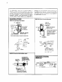
ROADSIDE
Either the direct or the reflex sensing mode may be
used for the roadside mounting arrangement. If th~ direct
mode is used, the transmitter and receiver must be placed
on opposite sides of the lane or roadway. If the reflex
mode is used, the sensor may be S2 or S3, and the retroreflector may be placed either on the pavement (Rl or
R2) or on the opposite side (R3). With the units on opposite sides, there will be some mistakes if there is more
than one lane of traffic and if vehicles interrupt the
beam(s) simultaneously. This arrangement is recommended only if the traffic volume is low. It is, however,
the required arrangement for measuring vehicle height. If
two sensors are used in this arrangement. direction can be
detennined by knowing which beam is broken fIrSt.
When the reflector is on the pavement, the infrared
beam is at an angle to the vertical. If only one beam is
used, it will be difficult. if not impossible, to place the
beam so that all passenger cars and all large trucks will
break it One beam would not be able to detect both a
low car near the shoulder edge and a truck with high
clearance near the lane line. Therefore, two or more sensors should be used at different levels with their output
signals connected with a logical OR to give more coverage and accurately sense all vehicle types.
Some combination vehicles may interrupt the light
beam more than once and be counted as more than one
vehicle, as in a manner similar to the overhead arrangement previously described. A solution to this problem
might be to use a sensor with a time delay as stated
above.
If the sensor is close enough to the edge of the
pavement, it is possible for specular reflections from
highly polished cars to give a false signal. This problem
was discovered while data were being collected on a
high-occupancy-vehicle (HOY) lane in Houston, where
some vehicles passed within about 4 feet of the reflex
sensor-receiver unit. A possible solution might be to use
a polarizing filter over the lens, but this approximately
OVERHEAD
Bridges or other overhead structures can be used to
mount infrared sensors, SI in Fig 4.1. The direct-sensing
mode is not well-suited for this arrangement since the
unit on the pavement surface, Rl, must have either a
power source or an external output connection, is difficult
to protect, and must be very rugged. A suitable retroreflector array has been designed for this purpose. In the
overhead arrangement, vehicles may be counted by lane,
and their speed and overall length may be calculated.
This is the only arrangement which can accurately sense
vehicles in lanes other than the outside lane or the median lane. Only specially-designed and placed retroreflectors are durable enough to be used directly on the
pavement for long periods of time.
51
52
"
·· ........
. .. .... ..
··.........
........
. ..
··.........
.........
· ......... ..
··.........
........ . ..
··.........
........ ..
· .........
........ ..
··.........
........ ..
··.........
~
-
-
-R3
- 55
R2
Fig 4.1. Sensor arrangements.
7
8
halves the sensing range. The manufacturer suggested
offsetting the retroreflectors from the sensors, i.e., using
diagonal light beams to cut the vehicle paths. Specular
reflections are strongest along the angle of reflection
which is equal to and opposite from the angle of
incidence. Therefore, if the sensors are offset by 15
degrees or more, they will not receive strong specular
reflection from flat reflecting surfaces parallel with the
lane lines.
PAVEMENT-LEVEL
When tires are being sensed, both sensors and relIOreflectors should be placed at the pavement level. The
beams are broken by the tires just as they contact the
ground and have their smallest cross-section. If the tires
were measured closer to their vertical centers, the sensors
might not have enough time to recover and count a
closely-following tire separately. For this reason, only
sensors with short response times should be used. The
through-beam sensing mode is not generally recommended for sensing tires for the reasons discussed previously with respect to overhead sensor mounting. For the
reflex-sensing mode, the retroreflectors should be placed
in the center of the lane so that tires on the same axle
straddle the retroreflector, and only the tires next to the
shoulder break the beam.
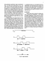
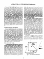
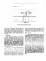
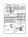
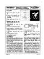
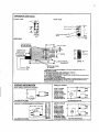
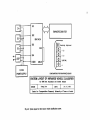
A three-sensor, pavement-level array is shown in Fig
4.2. 51,52, and S3 represent reflex sensors, while Rl,
R2, and R3 represent retroreflectors. 01, the distance between the two perpendicular beams, is used to measure
speed. 02 is the distance between the center of the lane
and the sensors, and 6 is the angle used to determine the
lateral position and the width of the tires. The retroreflectors are inside an inductance-loop detector in the center of the outside lane. The sensors are on the lane edge
or off the shoulder.
The signals from a two-axle vehicle, with respect to
time, are shown in Fig 4.3. S 1, S2, and S3 are the signals
received from the reflex sensors shown in Fig 4.2. A vehicle-presence signal is necessary for the tires to be
matched to the correct vehicle. A presence signal may be
generated by a separate infrared-beam array which senses
the vehicle body, or by another presence sensor such as
an inductance-loop detector. When a loop detector is
used, the retroreflectors are normally placed on the pavement inside the loop, as shown in Fig 4.2, so that the
presence signal begins before the first tire is sensed and
ends after the last tire is sensed.
Speed is calculated by dividing the distance between
the perpendicular infrared-light beams, 01, by the time
taken for one tire to travel between beams, time tv, shown
in Fig 4.3. If it is asswned that the vehicle and all tires
are traveling at a constant speed, then speed may be determined in a similar manner with a second loop detector,
two piezoelectric cables, or two WIM transducers. Axle
spacing is calculated by multiplying the speed by the
time between successive breaks of one beam, time ts.
Tire-contact length can be calculated by multiplying
the speed by the time that a perpendicular beam remains
broken by one tire, time 11. Tire-contact length is measured more accurately when the sensor is placed on the
pavement at the edge of the lane so that the beam size is
smaller and response is quicker. The retroreflector
should be small in size to further reduce the effective
beam size.
Other quantities may be measured with an infraredlight beam aimed diagonally across a vehicle path as
shown in Fig 4.2. When the speed is known, the lateral
distance of the tire from the center line or edge can be determined as a function of the time when a tire breaks the
diagonal beam and the time when that tire breaks a perpendicular beam, time tp, or crosses some other threshold, e.g., a weigh-in-motion transducer.
The projected diagonal dimension of the tire-contact
area is calculated similarly to the tire-contact length, except the interruption time of the diagonal beam, time td,
is used. The diagonally-measured dimensions of tires of
the same vehicle can be compared to give an indication
of single or dual tires. The rust tires of a vehicle are assumed to be single; following tires of the same vehicle
Loop Detector
R1
R2 R3
a
41:> a
/
I
/~
/
D2
-
--
I
I
I
1
-I/
I
I
I
/
/
a
a~
53
51 52
I-
D1
-I
Fig 4.2. Pavement-level sensors.
9
having dimensions significantly longer are indicated as
dual. The vehicle with the signal shown in Fig 4.3 has
single tires on the front axle and dual tires on the rear
axle. A factor of 1.2 has been found to be sufficient to
distinguish between the diagonal dimensions of single
and dual tires; i.e., diagonal dimensions of dual tires are
at least 1.2 times longer than single tires on the same vehicle. This factor is a variable in the computer program
which can be changed to account for different field conditions or observations. Output using the values of 1.1,
1.5, and 1.8 was compared with visual observations of
approximately twenty vehicles with dual tires. The 1.1
factor was not acceptable; the larger factors were acceptable but not optimal.
A different method with diagonal beams has been
used to distinguish between single and dual tires. Two
beams at a 45-degree angle to the center line and 23
inches apart may be used to calculate speed and axle
spacing in the manner previously described. Single tires
interrupt only one beam at a time, while dual tires interrupt both beams simultaneously. In field tests performed
on the Turner Turnpike outside Oklahoma City, the 23inch distance was found to be critical. For closer spacings, some single tires broke both beams at once, and, for
larger spacings, some dual tires broke the beams one at a
time. At the 23-inch distance, only a few small dual tires,
LO~
S1
Le., pickup-truck dual tires, were identified incorrectly.
Approximately twenty large trucks and five pickup truc,ks
with dual tires were visually observed and compared wlth
the output for each distance tested If this method were
to be combined with the diagonal dimension method.
then almost all vehicles should be classified correctly except motorcycles.
SUMMARY
Infrared sensors can be mounted in overhead, roadside, or pavement-level arrangements. In the overhead
and roadside arrangements, vehicle bodies are detected.
and vehicle speed, length, and headway can be measured.
In the pavement-level arrangement, vehicle tires are de·
tected, and vehicles can be classified according to the
number of axles per vehicle, the axle spacings, and the
sizes of the tire-contact areas. The infrared-light beams
can be perpendicular or diagonal to the lane edge, Diagonal beams are used to measure tire-con tact-area dimensions and the lateral position of tires. A presence
sensor, usually an inductance-loop detector, is required to
match tires with the correct vehicles. The next chapter
discusses how infrared sensors in these arrangements can
be applied for counting, classifying, and weighing vehicles.
L
Vehicle Presence
r--l~
______~
ts
S2
tp
S3
TIME
...
Fig 4.3. Signal relations.
CHAPTER 5. APPLICATIONS
Infrared sensors can be used for traffic counts, overheight detection, speed surveys, and vehicle classification. They can also aid weigh-in-motion measurements
by giving the lateral position of tires with respect to tireforce transducers. The reflex-sensing mode can be used
in all cases. In the direct-sensing mode, the sensor may
be mounted in the roadside position if the receiver is
mounted on the opposite side of the lane(s). The diffusesensing mode is not currently considered to be suitable
for sensing vehicles. Infrared-light sensors have distinct
advantages, but visible-light sensors can also be used.
height Two or more sensors should be mounted at different heights depending on the level of reliability desired. Infrared sensors can warn drivers of over-height
vehicles that they are approaching a low-clearance bridge
or tunnel. This system has been used in Mississippi and
other states (Ref 9). The direct-sensing mode should be
used because it has greater reliability than reflex sensing.
An application that is being considered is detecting trucks
on a ramp and warning the drivers if they are going too
fast and might be at risk of overturning.
SPEED
VEHICLE PRESENCE
Two infrared sensors are necessary for measuring
speed. Speed is equal to the distance between sensors divided by the time between successive beam interruption.
Sensors mounted overhead or on the roadside measure
vehicle speed, while pavement-level sensors measure
axle speeds which can be averaged for the vehicle speed.
The presence signal required for matching tire signals to the correct vehicles can be given by a pair of infrared sensors mounted overhead or on the roadside. The
first presence sensor should be located upstream from the
tire sensors, and the second presence sensor should be
downstream. The output signals of the two presence sensors should be connected with a logical AND. Infrared
sensors mounted on the pavement surface at the lane
edge have been used in a bridge research study to detect
approaching vehicles and indicate the lane of operation iii
advance of the instrumented bridge (Ref 8). Tape
switches had been used earlier but required closing lanes
and re-taping after rain. 1l1e lenses of the infrared sensors and retroreflectors can be wiped clean without closing lanes.
CLASSIFICATION
Classification can be done in a number of ways depending on the desired classification scheme. One pavement-level infrared sensor and a presence sensor can be
used to count the number of axles per vehicle. Two pavement-level sensors measure the axle spacing and indicate
whether axles have single, tandem. or triple spacing. If
an indication of dual or single tires is desired. the infrared
beams can be aimed diagonally across the lane rather
than perpendicularly. Alternatively. the first two beams
may be perpendicular and a third beam diagonal. If overall vehicle length is desired, an additional sensor should
be mounted on the roadside or overhead to detect the
presence of the vehicle body. If vehicle height is desired,
an array of sensors should be mounted at different heights
along the roadside. Any of these arrangements can be
used to distinguish between passenger cars and trucks.
COUNTING
Only one infrared sensor is necessary for counting
vehicles or tires, though an array of sensors may be desirable. Overhead or roadside-mounted sensors may be
used instead of inductance-loop detectors to count vehicle
bodies. Infrared sensors mounted at the pavement level
may be used instead of pneumatic road tubes or piezo
cables to count tires or axles.
WEIGHING
DIRECTION
Trre-contact area multiplied by tire inflation pressure
is an approximation of the downward force or weight of a
tire if the pressure is uniformly distributed. Many other
factors such as pavement roughness. speed. and
suspension systems affect the dynamic tire force.
Pavement-level infrared sensors can measure tire-contact
lengths and calculate widths of tires on a moving vehicle.
Field evaluations showed that tire-contact lengths
measured by infrared sensors compared favorably with
those measured statically, but widths did not (see Chapter
6). Tire-contact areas and, consequently, weight can be
estimated only roughly by infrared sensor measurements.
The direction of a vehicle can be determined when
two infrared sensors are used. Roadside or overhead
mounting is recommended. but pavement-level mounting
may also be used. When a vehicle breaks the beams in
the wrong order, a warning of wrong-way travel may be
given to the driver. This application may also be used for
directional traffic counts on lightly-traveled, two-way
roads.
VEHICLE HEIGHT
Infrared sensors mounted on the roadside may measure the height of vehicles or at least give the range of
10
tt
Lateral position of tires from the edge of the pavement can be measured with infrared sensors. This information can be used to detect tires passing off the edge of
WIM transducers. Lateral position measurements can
also be used to estimate the percentage of loads running
on or near the pavement edge.
SUMMARY
Infrared sensors can be used in several transportation
engineering applications. Single sensors may be used to
count vehicle bodies or axles. Other applications require
an array of two or more sensors. Infrared sensors can detect wrong-direction or over-height vehicles. They can be
used to classify vehicles according to number of axles per
vehicle, axle-spacing pattern, and single or dual tire configuration. Infrared sensors can measure tire-contact-area
dimensions and lateral position of tires in the traffic lane.
These measurements can be used to supplement infonnation from weigh-in-motion systems. The following chapter discusses field evaluations of several infrared-sensor
arrangements and applications.
CHAPTER 6. FIELD EVALUATIONS
Five major field tests of infrared sensors were perfonned between 1988 and 1990. The objectives were (I)
to detennine the feasibility of improving or replacing current vehicle counting and classifying systems and (2) to
explore the possibility of detennining vehicle weight using infrared sensors. In San Marcos, Texas, in September
1988, tire-contact-area dimensions were measured manually and compared to infrared-sensor measurements of
tires on moving vehicles. In December 1989, near Junction, Texas, tires were measured by infrared sensors and
weighed simultaneously with WIM transducers. In May
1990, in Houston, a two-beam infrnred-sensor array was
field tested as a possible substitute for loop detectors.
Sensors were installed at Jarrell, Texas, during the summer of 1990 to test their long-tenn perfonnance. In August 1990, in Oklahoma City, the possibility of using two
diagonal light-beam sensors to indicate single or dual
tires and classify vehicles was tested. All field tests were
perfonned on interstate highways. Except for the HOV
lane in Houston, all tests were in rural or semi-rural areas.
the lane edge measured vehicle speed and tire-contact
length, while a diagonal beam measured a projection of
the diagonal dimension of the tire-contact area, as shown
in Fig 6.1. Assuming a rectangular shape for the tirecontact area, the length and projected diagonal dimension
were calculated by multiplying vehicle speed by the time
of beam interruption for each tire. Width was computed
by subtracting the length from the projected diagonal
dimension, then dividing this remainder by the tangent of
the angle between the diagonal and perpendicular beams.
Static tire-contact lengths and widths were measured
directly with the special calipers.
The axle spacings measured by infrared sensors and
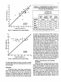
tape corresponded closely, which implied that speed calculations were accurate. The lengths and widths of the
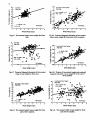
tire-contact areas are shown graphically in Figs 6.2 and
6.3 and are summarized in Table 6.1. If there were perfect agreement between the two sets of measurements
shown in the figures, all data points would fall on the 45degree line. The length values agree more closely than
the width values. The widths measured manually are
closely spaced around 21 inches, while the widths measured in motion are more widely dispersed around 19
inches. The tire-contact area for moving vehicle tires
changes and is not the same as the static tire-contact area.
Neither the dynamic nor the static tire-contact patch has a
rectangular area, as is assumed for the in-motion width
calculation. For dual tires, the width of the tire-contact
area includes the gap between tires and is greater than the
tire-contact length.
One reason for doing this test was to determine a
correction factor for the gaps between dual tires, which
could not be measured by infrared sensors. Gap size depends on tire size, construction, materials, and inflation
pressure; vehicle design; and other factors. Because of
EQUIPMENT AND SOFTWARE
The two brands of sensors used in the research described herein were manufactured by Banner and Opcon
(Refs I and 2). Some sensor housings were manufactured by Rainhan Co., 604 Williams Street, Austin, TX
78752, and others were fabricated at The University of
Texas at Austin. The retroreflectors were manufactured
by Stimsonite and 3M. In the field tests, a portable or
convertible IBM computer was used. Motorola donated
several evaluation boards and microprocessors that were
used to collect the raw data, make time lists, and communicate with the computer. A research engineer on the
staff of the Center for Transportation Research, The University of Texas at Austin, wrote all the software and developed support hardware for the microprocessor.
TIRE-CONTACT AREA
/
Width
A field study of tire-contact areas was conducted on
Interstate 35 near San Marcos, Texas, in September 1988.
Infrared sensors measured speed, axle spacings, tirecontact lengths, and diagonal dimensions of tire-contact
areas while vehicles were in motion. Vehicles were then
stopped by Department of Public Safety personnel. The
length and width of the tire-contact area was measured
manually by calipers built on a meter stick, and axle
spacings were tape measured. For the in-motion
measurements, infrared sensors were set at the edge of
the shoulder and aimed at retroreflectors in the middle of
the adjacent lane. Two infrared beams perpendicular to
/
/
IR Beam, /
TIme 2 /
/
/
/
I
/
/
/
\
..
Length
/
/+
1\
,.~--------.,~~
Projected Diagonal Dimension
Fig 6.1. Tire-contact-area dimensions.
12
/
/ IR Beam,
TIme 1
/
/
/
/
Travel
13
13
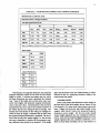
TABLE 6.1. COMPARISON OF TIRE-CONTACT
LENGTH AND WIDTH MEASURED MANUALLY
BY TAPE AND BY INFRARED
12
11
c::
;=:..
.c
•
10
0)
c:
Q)
....J
9
•
Q)
~
i=
8
c:
7
co:::l
co
•
•
•
:::i!:
6
All Dual Tires
Dimensions (in.)
Length
IR
Number
35 Vehicles
Dual TIres
5
4
4
5
6
7
8
9
10
11
12
13
Infrared Tire Length (in.)
23
•
"'":' 21
g
-
.c
~ 20
• • ••• ••••
• •••• • •
•
....
co
Q)
i= 19
~
c:
co
:::i!: 18
29 Vehicles
17
Dual Tires
16
16
17
18
19
20
21
22
35 Tires
Width
IR
Width
Manual
29 Tires
Min
4.5
6.7
16.19
20.08
Max
12.3
12.2
21.97
22.13
Mean
9.9
9.7
19.37
21.18
Std Dev
1.7
1.3
1.63
0.42
Tire-contact width includes gap between dual tires.
Fig 6.2. Comparison of tire-contact lengths.
22
Length
Manual
23
Infrared Tire Width (in.)
Fig 6.3. Comparison of tire-contact widths.
the rather large amount of scatter in the data, a suitable
correction factor could not be determined from the available information.
WEIGHT
In December 1989, a three-sensor, pavement-level
sensor array was field tested on Interstate 10 at Junction,
Texas. The objective of this test was to determine the
possibility of estimating weight from measurements of
in-motion tire-contact-area dimensions. The sensors were
installed on the edge of the lane, and the beams passed
just above a flush-mounted Radian WIM transducer in
the right-side wheel path so that tire-contact length and
projected diagonal dimension could be measured as each
right-side tire was being weighed. Both systems shared a
loop detector to sense vehicle presence but computed
vehicle speed and axle spacing independently. The
infrared-light-beam system also calculated the tirecontact length, projected diagonal dimension of the tirecontact area, and the lateral position of the tire with
respect to the edge of the pavement. All calculations
were done on-site with a portable microcomputer. Both
the infrared sensors and retroreflectors were smaller and
closer together than those used in the test at San Marcos.
The retroreflectors were 3/4-inch-diameter rather than 4inch-long raised pavement markers as were used before.
The infrared sensors were placed on the lane edge rather
than off the shoulder. The new sensors had a range of
about 20 feet rather than 50 feet. This arrangement
reduced the size of the effective beam and thus enhanced
the measurement accuracy of tire-contact dimensions.
SPEED, AXLE SPACING, AND LATERAL
POSITION
Figures 6.4 and 6.5 compare the speed and axle spacing for infrared sensors and WIM, while Table 6.2 summarizes this information. In this test, speeds measured
by infrared sensors were slightly higher than speeds measured by WIM, as shown by the data points above the 45degree line in Fig 6.4. The speed measurements for the
WIM system were made with two 6-foot-by-6-foot loop
detectors separated by an 8-foot space. These two loops
were not calibrated perfectly, and their response times
were inherently affected by the different heights of the
14
vehicles above the road surface. The axle spacings from
the two measuring techniques show close agreement, but
the effect of higher speed, computed from the infrared
sensors, makes the corresponding axle spacings lie above
the 45-degree line in Fig 6.5. The speeds calculated from
the infrared-sensor measurements are probably more reliable than those from the loop detectors.
The lateral position of tires from the lane edge were
measured by the diagonal infrared beam. This
measurement determined whether vehicle tires were fully
supported by the WIM transducer. Measurements
resulting from all off-transducer vehicles were excluded
from this analysis. A summary of field measurements is
shown at the bottom of Table 6.2.
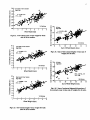
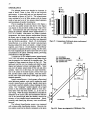
Figures 6.6 through 6.15 present tire-contact-area dimensions of various tires, or sets of tires,versus weight.
All dimensions and weights are for the right-side tires.
Tire-contact lengths, projected diagonal dimensions of
tire-contact area, and weights are summarized in Table
6.3.
FRONT AXLE
75
Figure 6.6 presents tire-contact length versus weight
for front axles. A least-squares regression line of these
data points is shown, assuming that weight is the independent variable. Dynamic measurement of tire-contact
length is probably accurate to within about ± 1 inch,
slightly more than the standard deviation for the front
axle, 0.8 inches. The regression line is valid only for observed tire-contact lengths from about 16 to 18 inches,
while weights ranged from about 2,500 to 5,500 pounds.
Therefore it is not feasible to estimate weight adequately
from dynamic measurement of tire-contact length. The
standard deviation of tire-contact length for the front axle
is smaller than that for the other axles, but tire-contact
length is a poor estimator of weight.
Projected diagonal dimension versus weight for front
axles is shown in Fig 6.7. A least-squares regression line
is shown, assuming that weight is the independent variable. The regression line is valid only for projected diagonal dimensions between 17and 20 inches, while
weights ranged between 2,500 and 5,500 pounds. The
standard deviation, 2.6 inches, is greater than the expected accuracy, about 1 inch; therefore, it is not appropriate to use the projected diagonal dimension of the tirecontact area to estimate weight. Evaluation of the data
shown in these two figures indicates that wheel weights
cannot be estimated from the tire-contact lengths nor projected from diagonal dimensions with acceptable accu-
Speed
70
65
:co.
-...
E 60
"0
Q)
-
~ 55
c:
50
45
149 Vehicles
40
40
45
55
50
60
65
75
70
Weigh-in-Motion (mph)
Fig 6.4. Comparison of speed.
60
Axle SpaCing
596 Axle Pai 15
racy.
g
...
~ 30
-.s
~
20
O~
o
____L -____L -____L -_ _
10
20
30
~~
40
__
~
____
50
Weigh-in-Motion (tt)
Fig 6.5. Comparison or axle spacing.
~
60
The front-axle tires had longer contact lengths than
the tandem-axle (dual) tires. As expected for single tires,
the projected diagonal dimensions of the front-axle tires
were considerably shorter than those of the tandem-axle
tires, which were all dual. Some of the front-axle tires, in
fact, had measured in-motion lengths longer than their
projected diagonal dimensions. The technique described
in the previous section for calculating tire-contact width
yielded negative values for tire-contact widths in these
cases. The dual tires all had measured in-motion lengths
less than the corresponding projected diagonal dimensions. Analysis of the field data indicated that the calculated tire-contact width for tires on tandem axles was not
correlated strongly enough with weight to serve as as an
adequate weight-estimation basis.
15
TABLE 6.2. AXLE SPACING, SPEED, AND LATERAL POSITION
Measurements at Junction, Texas
Infrared Sensors vs Weigb·ln.Motion
Axle Spacing Dimensions (rt)
IR
WIM
IR12
IR23
IR34
IR45
WIM12
WIM23
WIM34
WIM45
Min
9.13
4.11
23.39
3.89
8.80
3.90
25.70
3.60
Max
21.03
4.90
53.39
4.17
20.20
4.90
51.70
4.10
Mean
15.10
4.31
31.35
4.02
14.57
4.18
30.31
3.90
2.94
0.07
3.25
0.06
2.83
0.11
3.11
0.09
Std Dev
IR12 and WIM12 represent the spacing between the first and second axle. etc.
Speed (mpb)
IR
WIM
Min
43.79
43.00
Max
70.24
67.00
Mean
60.18
57.38
4.70
4.39
Std Dev
Lateral Position (In.)
Min
26.12
Max
38.22
Mean
30.34
Std Dev
3.21
Theoretically, the diagonal dimension and projected
diagonal dimension cannot be less than the tire-contact
length or width. A circular tire-contact area, for which
all these dimensions are equal, represents the limiting
case. Some of the single tires on front axles were measured with lengths and projected diagonal dimensions
close to the same value. Inconsistencies in the in-motion
measurements are due in part to the dynamic behavior of
the vehicle and the tires during the time of sensing. The
location and cross-section of the rolling tire changes between the time the length is measured and the time when
the projected diagonal dimension is measured. The elevation of the tire may also change slightly, i.e., the tire may
ride into a depression or bounce off the pavement, causing a different cross-section to be measured. If the height
above the pavement of the two infrared beams is slightly
different at the two measuring locations. different tire
cross-sections are sensed.
TANDEM AXLES
Plots of tire-contact area dimension versus weight for
the front axle of the drive-tandem set are shown in Figs
6.8 through 6.12, along with least-squares regression
lines. Figure 6.8 shows the tire-contact length versus
weight, while Fig 6.9 shows the projected diagonal
dimension versus weight. For the tire-contact length
versus weight regression line, the correlation coefficient
is 0.67, while for the projected diagonal dimension versus
weight regression line, the correlation coefficient is 0.70.
There is some linear correlation, but it is not sufficient to
16
20
19
_
c:::
~
18
oc:
17
...J
16
.c:
a>
t>
30
Front Axle
Right Side
29
POD = 0.582W + 23.4
R~2" 0.70
-:5 28
01
c:
CI:I
27
...J
S
15
~
8
14
'e
c:
~
13
26
0...
L = 0.527W + 15.0
RA2=0.13
12
•
149 Vehicles
11L-~~~--~--~--~--~--~~
1
2
3
456
7
8
2
9
4
3
550
g
<I)
c: 19
0
'ii)
c: 17
a>
E
is 15
•
•
"iii
0
6
7
9
8
Front Axle
Right Side
-:- 21
01
5
Fig 6.9. Projected diagonal dimension of tire-contact
areas versus weight for front axle of drive tandem.
Fig 6.6. Tire-contact length versus weight for front
axle.
23
149 Vehicles
Wheel Weight (kips)
Wheel Weight (kips)
c:
•
Front Axle of Drive Tandem
Right Side
POD = 0.459W + 16.8
RA2= 0.009
13
C'CI
•
is 11
9
•
~
#
.
~o
4
P = 22.6W + 299
RA2= 0.72
450
01
co
••
•
i:5
400
I<
.c:
g 350
~
149 Vehicles
3
2
c:r 500
.!!t
~:
•\ •• t·
'••
Front Axle of Drive Tandem
Right Side
5
149 Vehicles
300
1----11...-.......' - - - - '_ _- - 1 0 _......._
34567
2
1
6
_....1._
. . 9.
8
......
Wheel Weight (kips)
Wheel Weight (kips)
Fig 6.7. Projected diagonal dimension of tire-contact
areas versus weight for front axle.
Fig 6.10. Product of tireo(ontact length and projected
diagonal dimension versus weight for front axle of
drive tandem.
-
Front Axle of Drive Tandem
Right Side
~
-
"0
oc:
16
1:)
...J
15
J9
c:
14
uI
~
.c:
a>
....
CI:I
~
WD :0.121W +16.2
RA2 =0.045
-:- 19
18
17
c:::
Front Axle of Drive Tandem
Right Side
20
20
•• •
•
.c: 18
~
0
17
16
....
<1:1
13
11
~
L=0.505W+ 13.1
RA2 = 0.67
12
15
14
1
2
3
4
••
149 Vehicles
5
6
7
8
9
Wheel Weight (kips)
Fig 6.S. Tire-contact length versus weight for front
axle of drive tandem.
1
2
3
4
5
149 Vehicles
6
7
8
Wheel Weight (kips)
Fig 6.11. Tire-contact width versus weight for front
axle of drive tandem.
9
17
340
Front Axle of Drive Tandem
Right Side
:? 320
•
CT
..!:2. 300
A,. 10.3W +210
RA2 = 0.60
ell
C'CI
E 280
«......
(.)
C'CI
260
t:
0
Q
240
I
E
i= 220
200
149 Vehicles
2
1
95
All Axles
Right Side
ell
3
4
567
8
9
S01
L =0.547W + 66.6
R"2 = 0.72
t:
Wheel Weight (kips)
~ 85
tS
S
Fig 6.12. Tire-contact area versus weight ror tront
axle or drive tandem.
t:
0
Q
I
....
a:>
i=
•
'0
E 65
:::::I
20
§..
(I)
Front Axle of Drive Tandem
Right Side
19
18
15
10
25
20
30
35
40
Sum of Wheel Weights (kips)
L =0.505W +13.1
R"2 =0.67
S17
g'
149 Vehicles
Fig 6.14. Sum or tire-contact lengths versus sum or
weights for all axles.
~ 16
......
(.)
S
15
•
t:
0
Q
I
a:>
~
13
All Axles
en
12
11
Right Side
t:
149 Vehicles
0
'CiS
t:
1
2
3
4
5
6
7
8
9
Wheel Weight (kips)
a:>
E
is
1i
t:
POD =0.671W + 107
n:s 110
R"2 =0.64
0
01
20
-
19
:.::. 18
S 17
t:
t:
a:>
......
(.)
.e
t:
(I)
10
••
•
•
15
20
149 Vehicles
25
30
35
40
Sum of Wheel Weights (kips)
Fig 6.15. Sum or projected diagonal dimensions of
tire-contact areas versus sum of weights ror all axles.
15
14
'-
13
i=
E
:::::I 100
16
0
Q
I
a:>
'0
•
L = 0.566W + 12.8
R"2 =0.71
01
-J
is
Rear Axle of Drive Tandem
Right Side
12
11
149 vehicles
1
2
3
4
5
6
7
8
Wheel Weight (kips)
Fig 6.13. Tire-contact length versus weight ror both
axles or drive tandem.
9
18
TABLE 6.3. SUMMARY OF TIRE·CONTACT AREA
AND WEIGHT
149 Five·Axle Seml-TraUerTrucks Right Side Only
Tire Length
(In.)
Minimum
Maximum
Mean
Sui Dev
Axle
_1_
15.40
19.48
17.15
0.76
Axle
2
13.47
18.20
16.07
1.05
Axle
3
13.15
18.39
15.96
1.10
Axle
4
12.84
18.46
15.82
1.30
Axle
5
11.96
19.26
15.99
1.29
Tan·
dem 1
26.62
36.00
32.03
2.10
Tan~
25.06
37.26
31.81
2.51
Axles
69.15
90.88
80.99
4.79
9.03
22.03
18.73
2.63
24.26
29.65
26.88
1.18
23.97
29.33
26.81
1.12
20.73
29.13
26.23
1.63
20.73
28.90
26.23
1.61
48.24
57.51
53.68
2.23
41.47
56.99
52.46
3.18
104.64
135.08
124.88
6.21
2,528
5.544
4.145
527
2.008
8.504
5.903
1.698
2.128
8,344
5.639
1,640
1.288
9,424
5,229
2,123
1.296
9.936
5,380
2.087
4.136
16.464
11.542
3,292
2.680
17.560
10.608
4,133
10.984
35.848
26.295
7.423
All
Projected
Diagonal
Dimension
(In.)
Minimum
Maximum
Mean
StdDev
Weigbt
!Ib~
Minimum
Maximum
Mean
SrdDev
estimate weight from infrared-sensor measurements with
reasonable accuracy.
In an attempt to explore other possible weight-estimation techniques from infrared-sensor measurements.
the plots shown in Figs 6.10. 6.11. and 6.12 were generated. Figure 6.10 presents the product of tire-contact
length and projected diagonal dimension versus weight.
The correlation coefficient for the product is 0.72, only
slightly higher than the values of 0.67 and 0.70 for the
two factors taken individually. Figure 6.11 presents the
tire-contact width versus weight The tire-contact width
was calculated by subtracting the tire-contact length from
the diagonal dimension and dividing by the tangent of the
angle between the perpendicular and the diagonal infrared beams. This calculation assumes a rectangular tirecontact patch. This assumption is perhaps more appropriate for dual tires than for single tires, since all the
calculated widths were positive for dual tires. With the
poor correlation obtained, calculated tire-contact width
cannot be used to estimate weight satisfactorily. Figure
6.12 presents the calculated tire-contact area, i.e., the
product of tire-contact length and width. versus weight.
The linear correlation is again poor. None of the dependent variables described here can be used to estimate
weight with reasonable accuracy.
The tandem axles were found to be similar to each
other when tire-contact lengths and projected diagonal dimensions were compared, as can be seen from the values
in Table 6.3. The tire-contact length for the drive tandem
had standard deviation values of 1.05 and 1.10 inches,
while the trailer tandem had standard deviation values of
1.30 and 1.29 inches. The projected diagonal dimension
for the drive tandem had standard deviation values of
1.18 and 1.12 inches. while the trailer tandem had values
of 1.63 and 1.61. The mean values of tire-contact length
for both tandem axles were very close. between 15.82
and 16.07 inches. The mean values of projected diagonal
dimension for each tandem were very close, 26.88 and
26.81 inches for the drive tandem, and 26.23 inches for
both axles of the trailer tandem.
Figure 6.13 compares the regression lines of tirecontact length versus weight for the front and rear axles
of the drive tandem. The lines are very similar, with
slopes at 0.505 and 0.566 and the intercepts at 13.1 and
12.8. Since the axles have a common suspension point, it
is expected that the weights will be similar. The data
taken in this field test show that the tire-contact area dimensions are also similar.
AU AXLES
In Figs 6.14 and 6.15, the dimensions of all the tires
on each vehicle are summed. The least-squares regression lines and correlation coefficients are also shown.
Figure 6.14 presents the sum of all the tire-contact
lengths versus the sum of all the weights. Figure 6.15
presents the sum of the projected diagonal dimensions
19
12 ft Main Lane
-__t
__
Piezo Gable
12 ft Main Lane
10ft Shoulder
- "X8R~
,,
," ,
Loop
.,.
'fr
'"
'"
/"
T
''
I
,
,
'1'
,
,,
I
----------~~-~--~---~--ReHex Sensors
Fig 6.16. Sensor arrangement at JarreD.
versus the sum of the weights. The correlation coefficients are 0.64 for tire-contact length versus weight and
0.72 for projected diagonal dimension versus weight. It
might be possible to indicate whether trucks are empty or
loaded, but the accuracy is insufficient to warrant any further study at this time. Accurate estimation of weight is
not feasible.
SUMMARY
The tire-contact-area dimensions of the front axle are
very poorly correlated with the weight. The tire-contact
lengths and projected diagonal dimensions have similar
values, indicating that the tire-contact patch for single
tires is close to circular. Many of the front tires had
lengths longer than the projected diagonal dimension,
partially due to dynamic forces acting on the tire. A rectangular tire-contact patch is assumed for the tire-contact
width calculation. This assumption is not valid, especially
for the front tires. Values calculated for width are not
correlated with weight.
On the plots for tire-contact length and projected
diagonal dimension versus weight for the tandem axles,
there are two defmite clusters of data points representing
the empty and loaded trucks. However, the accuracy is
not adequate even for estimating weight to within 10,000
pounds. Closer estimates of weight do not seem to be
possible at this time. More information is needed than
can be sensed by infrared sensors, i.e., tire pressures and
shapes of the tire-contact patches. If remote tire-
pressure-sensing technology were developed, infrared
sensors could be used to calculate the weight of vehicles
quite accurately. For the present, infrared sensors are not
recommended for calculating individual vehicle weights.
HOVLANES
A two-beam infrared-sensor array was field tested in
a high-occupancy-vehicle (HOV) lane on Interstate 10 in
Houston in May 1990. The two reflex-type infrared sensors were placed 2 feet apart in a special metal box on
top of one concrete median barrier; the retroreflectors
were placed on the nearly-vertical face of the other barrier 22 feet away. This system was tested as a possible
substitute for an array of inductance-loop detectors that
are currently used to determine vehicle speed, length, direction, and headway in the reverse-flow HOV lane. The
system performed well for the fIrSt two weeks, until the
lid on the metal box became ajar and road fIlm accumulated on the lenses. It is felt that a sensor unit of this type
will perform well over extended periods of time after a
few minor modifications to the mounting hardware are
made. Occasional cleaning of the lenses and retroreflectors may be necessary. Only minor modification of the
currently-implemented computer software is required before a single pair of infrared sensors can be used to replace the existing array of three 6-foot-by-6-foot loop detectors.
20
o IR
ENDURANCE
Five infrared sensors were installed on Interstate 35
north of Jarrell. Texas. in June 1990 to test long-term
performance. A piezo cable and two loop detectors were
also installed. as shown in Fig 6.16. The infrared-sensor
array consisted of a set of three sensors with the beams
inside a loop and a set of two sensors placed upstream
and downstream of another loop detector.
Prior to installing the sensors shown in the figure. a
set of five low-profIle sensors (not shown in the figure)
was placed on the pavement surface at the edge of the
lane. Cast-aluminum and epoxy housings were used to
protect the miniature infrared sensors (approximately 1.5
X 2.0 X 0.5 inches). After about two weeks in summer
temperatures, the sensors became nonfunctional because
the beams were no longer high enough to crest the high
point beside the wheel-path rut since they were depressed
into the flexible pavement. Small, l/2-inch-diameter
retroreflec tors , in a similar but smaller cast-aluminum
housing, endured for about two months. A larger circular
segment. sawn from a 1.5-inch-diameter retroreflector
and housed in a special aluminum casting, was first used;
but water migrated past the epoxy seal of the saw-cut and
accwnulated on the plastic reflecting surface, preventing
retroreflection of the light beam.
A second set of five infrared sensors (approximately
2.0 X 2.0 X 4.0 inches) was placed on steel stakes driven
into the ground a few inches off the shoulder edge. The
locations of these sensors are shown in Fig 6.16. They
performed well for over two months and could be easily
aligned and adjusted without interrupting traffic. Metal
cans over the plastic sensors kept off the rain and direct
sunlight After two or three days, the small retroreflectors in the center of the lane became covered with road
fLlm, and the system could not operate. After the retroreflectors were wiped clean during a traffic gap, the system
reswned operation.
Larger retroreflectors, 4-inch-square reflectorized
raised pavement markers. were used to replace the small
circular retroreflectors, and under regular observation
were found to perform reliably without cleaning for three
weeks. Two "temporary" markers (Placed with a liquid
primer on the rubberized asphalt adhesive) were functional after more than three months, i.e., at the time of
this writing. While the larger retroreflectors extended the
endurance of the system, they also increased the effective
size of the infrared-light beam and thereby reduced the
accuracy of tire-contact-Iength measurements. Speed,
counting, and classifying accuracy were not affected,
however.
The infrared classification system was compared
with a piezo-cable classification system. However, the
two systems could not be directly compared, as the piezo
~ Piezo
350
•
Manual
300
CI)
c:
5
u
250
200
Q)
~ 150
100
50
2
3
4
5
Fifteen-Minute Periods
Fig 6.17. Comparison or inrrared, piezo, and manual
axle acounts.
o
o Retroreflector
-
•
~
Infrared Reflex Sensor
Inductance Loop Detector
Guardfence Post
TRAFFIC
•
•
72 In.
•
72 in.
12 It Shoulder
72 in.
12 It lane
Fig 6.18. Sensor arrangement at Oklahoma City.
21
system required both loop detectors shown in Fig 6.16,
and it was not possible for the loops to be used by both
systems simultaneously. Figure 6.17 shows a comparison
between axles counted by infrared sensors, piezo sensors,
and by three human observers. The three human observers never agreed exactly, so an average count is shown in
the figure. Except for period one, the infrared-sensor
axle counts were greater than the piezo-sensor axle
counts. Using the manual axle counts as a basis, the expected error for the piezo sensor was ten axles per 15
minutes, and for the infrared sensor, two axles per 15
minutes. This calculation is based on only five periods.
Infrared sensors can be used for long-term traffic surveys if proper precautions are taken to protect the sensors
and retroreflectors from the environmental effects. Environmental effects include rain, road film, temperature extremes, and shock and vibration from vehicles.
SINGLEIDUAL TIRE IDENTIFICATION
AND VEHICLE CLASSIFICATION
A system for classifying vehicles for auditing toll
collection was tested on Interstate 44 (Turner Turnpike),
in Oklahoma City, in August 1990. At the test site, about
500 yards downstream of a toll plaza, vehicles were traveling about 50 to 65 mph. The system included a loop
detector and two diagonal beam sensors and retroreflectors, placed 23 inches apart, as shown in Fig 6.18.
Single tires interrupted the beams sequentially, while
dual tires interrupted them simultaneously. It was found
by field observation that a distance of 23 inches between
infrared light beams was optimum. At a 22-inch distance, some large-diameter single tires were classified as
dual; while at 24 inches, some small-diameter dual tires
were classified as single. Generally, only the relatively
small-diameter dual tires of pickup trucks were identified
as single at the 23-inch distance. An initial value of 24
inches was established after measuring truck tires in a
parking lot In the field test, approximately twenty large
trucks were observed visually and compared with the
computer output based on 24 inches; several dual tires
were misidentified. At the 22-inch distance, several
single tires were misidentified. At the 23-inch distance,
almost all vehicles were identified correctly for approximately one hundred observations.
This system, using two diagonal beams a fixed
distance apart, was designed for use at toll gates where
speed of vehicles would not be constant. The tire-contact
length-diagonal dimension, three-beam system
described in Chapter 4--could not be used since constant
velocity is assumed. The system described here might be
improved with a three-diagonal-beam array. Tires
interrupting all three beams simultaneously would be
classified as dual; tires interrupting the first two beams
sequentially would be single; and vehicles interrupting
the first two beams simultaneously would be single or
dual depending on the classification of the other tires of
that vehicle. This proposed system has not been tested.
Under the Oklahoma Turnpike Authority Classification
Schedule, axle spacing is not a criterion, so a
classification system which does not assume constant
velocity can possibly be used.
In the field tests, off-duty toll-booth operators recorded vehicle classifications based on visual observations. The operators were required to identify the vehicle
class and press the appropriate computer key before the
vehicles activated the loop detector. The operator and infrared-system classification errors are summarized in
Table 6.4 (Ref 10). The operators were 94.7 percent successful, while the infrared system was 96.3 percent successful. Many of the operator errors were due to vehicles' following too closely, which made the time
available for pressing the computer key too short. The
system errors could be reduced by using a three-sensor
array, as described above, which could classify small dual
tires correctly.
TABLE 6.4. VEmCLE CLASSIFICATION
ERRORS ON OKLAHOMA TURNPIKE
Operator
Errors
System
Errors
Date
or Test
No. or
Vehicles
21 AUG 1990
120
6
5.0%
3
2.5%
1 SEP 1990
500
23
4.6%
11
2.2%
8 SEP 1990
502
37
7.4%
29
5.8%
14 SEP 1990
351
13
3.7%
10
2.8%
14 SEP 1990
260
12
4.6%
11
4.2%
Total
1733
91
5.3%
64
3.7%
SUMMARY
Five field tests of infrared sensors were performed.
The objective of the first two tests was to determine the
possibility of weighing vehicles with infrared sensors.
The objective of the other three tests was to determine
the feasibility of improving or replacing current vehicle
classification systems with infrared-sensor systems. In
the tire-con tact-area study performed at San Marcos,
Texas, it was determined that the tire-contact length but
not the width could be calculated with reasonable
accuracy from infrared measurements of vehicles moving
at high speeds. In the test at Junction, Texas, it was
determined that infrared sensors could estimate only
roughly the dynamic weight of vehicles by measuring the
tire-contact area. The lateral position of tires was also
measured. In these two tests it was demonstrated that
22
infrared sensors could accurately measure vehicle speed
and axle-spacing patterns.
In the HOV (high-occupancy-vehicle) lane test in
Houston, it was shown that infrared sensors can replace
inductance-loop detectors, which are currently used to
measure vehicle speed, length, and headway. In the
endurance test at Jarrell, Texas, it was shown that infrared
sensors can function for several months with minimal or
no maintenance. It was also demonstrated that axle
counts by infrared sensors are at least as accurate as axle
counts by piezo cables or human observers. In the
turnpike test performed in Oklahoma City, it was
demonstrated that infrared sensors can identify almost all
single and dual tires. Vehicle classifications by the
infrared-sensor system were as accurate as classifications
by off-duty toll-booth operators.
The cost of a reflex-type infrared-sensor and retroreflector unit is approximately $100. A traffic lane closure
is usually not required for installation of the unit. In
comparison, a piezoelectric cable costs approximately
$300, and installation requires closing a traffic lane and
sawing a groove. The infrared sensors examined in this
study were not tested to failure, so their life expectancy
and long-tenn reliability are not known.
CHAPTER 7. CONCLUSIONS
Infrared sensors may be used in a variety of traffic
studies. They can be installed to count and classify vehicles accurately without requiring pavement cuts or
bumps as do loop detectors or road tubes. Classification
criteria, which can be calculated with information obtained from infrared sensors, include number of axles per
vehicle, axle-spacing pattern, and single or dual tires. Infrared sensor information can also be used to calculate
overall length or height of the vehicle, speed, and headway. These data can supplement weigh-in-motion systems by identifying tires of vehicles not fully in contact
with the force transducers.
The reflex-sensing mode is recommended for most
traffic detection applications. The direct-sensing mode
may be used for over-height detection and other applications where the transmitter and the receiver are mounted
on opposite sides of the roadway. The diffuse-sensing
mode is not recommended for traffic applications.
Either roadside or overhead arrangements may be
used for sensing vehicle bodies, but the overhead arrangement must be used for sensing vehicles in lanes
away from the roadside. To reduce miscounting resulting
from gaps between vehicle units, sensors with a time delay may be used. For sensing vehicle height, an array of
sensors at different heights should be used in the roadside
arrangement Pavement-level sensors should be used for
sensing tires. The shoulder-edge location is recommended, especially for heavy traffic. The lane-edge location may be used for short-term applications of less than
about three days' duration or when retroreflectors and
lenses can be cleaned frequently.
Comer-cube retroreflectors are recommended for all
applications. Spherical-bead retroreflectors should not be
used if polarizing filters are used with the sensors.
Five major field tests were carried out to determine
the feasibility of using infrared sensors for counting,
classifying, and weighing vehicles. A tire-con tact-area
study was performed at San Marcos, Texas. In-motion
tire-contact area was calculated from infrared-sensor
measurements and compared with static measurements
taken manually. Static and dynamic tire-contact lengths
showed good agreement, but because the tire-contact
patch is not rectangular and constantly changes, the inmotion tire-contact widths did not agree very well.
Another study was performed at Junction, Texas, to
determine the feasibility of using infrared sensors to
weigh vehicles. Infrared sensors measured tire-contact
dimensions and WIM transducers measured wheel
weights simultaneously. It is not feasible to estimate
weight from tire-contact dimensions measured in motion.
Infrared sensors can be used to determine the lateral position of tires with respect to the WIM transducer, thus improving the performance of WIM systems.
A third field test was performed on an HOV lane in
Houston to determine the feasibility of replacing an array
of three inductance-loop detectors used for calculating
vehicle speed, length, direction, and headway with an array of two infrared reflex sensors. With minor modifications of the sensor housings and the current computer
software, infrared sensors can replace the loop detectors.
Five infrared sensors were installed near Jarrell,
Texas, to test long-term performance. For applications
longer than about a week, it is necessary to mount
pavement-level sensors off the shoulder to protect them
from the shock of heavy vehicles and the accumulation of
road film. Small retroreflectors used on the pavement
surface for measuring tire-contact dimensions accumulate
road film and must be cleaned every two or three days.
Larger retroreflectors or reflectorized raised pavement
markers may be used for measuring speed, counting, and
classifying.
The fIfth test was performed on the Turner Turnpike
in Oklahoma City, with the objective of identifying single
and dual tires and classifying vehicles for auditing toll
collection. Ninety-six percent of the vehicles were identified correctly with the array of two infrared sensors and
a loop detector. The accuracy can be improved with an
additional infrared sensor.
The cost of a reflex-type infrared sensor and
retroreflector unit is about $100, and installation can be
accomplished without pavement cuts, usually without
traffic barricades. Thus, infrared sensors are accurate and
economical alternatives to sensing devices currently used
to count and classify vehicles. Infrared sensors can also
be used with weigh-in-motion systems to sense offtransducer vehicles.
23
REFERENCES
1. Opcon Catalog of Photoelectric Controls, OPCON,
720 80th Street S.w., Everett, WA 98203, P 138,1984.
and Transportation Officials, Washington, D.
1990.
c.,
7. Standard Specification for Highway Weigh-in-Motion
(WIM) Systems with User Requirements and
Test Method, E 1318-90, American Society for
Testing and Materials, Philadelphia, 1990.
2. Banner Engineering Product Catalog, Banner Engineering Corporation, 9714 lOth Ave. No., Minneapolis, MN 55441,1987.
3. Photoelectric Sensors and Controls: Selection and
Application, Juds, Scott M., Marcel Dekker, Inc.,
New York, 1988.
8. Schulz, Jeff, University of Colorado, personal correspondence.
9. "Overheight Vehicle Warning Systems in Mississippi,"
Hanchey, Craig M., and Slade F. Exley, ITE
Journal, June 1990, pp 24-29.
4. Traffic Monitoring Guide, Federal Highway Administration, Office of Highway Planning, 1985.
5. Classification Schedule, Oklahoma Turnpike Authority.
10. Test of a System to Classify Vehicles for Toll Collection, Gattis, J. L., and Clyde E. Lee, Report to
Traffic Engineering Consultants, Inc., October
1990.
6. A Policy on Geometric Design of Highways and
Streets, American Association of State Highway
24
APPENDIX
Photographs and descriptions of the equipment and
circuit diagrams of the systems used in the field
evaluations are included in this appendix. Figure A.I
shows the metal box housing two Opcon infrared sensors
which was placed on top of a concrete median barrier on
one side of the Houston HOV lane. Figure A.2 shows
from left to right a loop detector, two Opcon reflex-type
sensors mounted on a tripod, a Motorola evaluation
board, and an IBM computer. The M68HCllEVBU
universal evaluation board manufactured by Motorola can
be used to process and store the output signals of infrared
sensors. The board is a single-chip microcontroller unit
which can operate programs down-loaded from an RS232C-compatible host computer. Space is provided on
the board for custom interfacing. The primary power
requirement is + 5.0 Vdc @50 rnA.
Figure A.3 shows a StreeterAmet traffic counter
(normally connected to a road tube) connected to an
Opcon sensor. A retroreflector is also shown. Figure AA
shows a cast-aluminum housing which can be mounted
on the lane edge; a Banner sensor is shown both inside
and next to the housing.
Figure A.5 shows an Opcon sensor mounted off the
shoulder edge on a metal stake. Figure A.6 shows three
different Banner sensors used in the field tests. At the
top left is a sensor with a built-in counter with liquidcrystal display. The sensor at the top right was used in
some preliminary tests. The sensor at the bottom was
used at Junction inside the cast-aluminum housing.
Detailed descriptions of the infrared sensors, shown
in Figs A.I through A.6, appear in the following pages.
Descriptions of the Opcon reflex sensor, the DC/NPN
control modules, and the three Banner sensors pictured in
Fig A.6 are included.
The OR gate circuit diagram used on the HOV lane
in Houston is shown in Fig A. 7. Figure A.8 shows the
system layout for the three-sensor vehicle classification
system used in the field tests at San Marcos, Junction,
and Jarrell. Figure A.9 shows the system layout of the
two-sensor vehicle classification system used in the Oklahoma City field test.
25
26
Fig A.I. Metal box housing two Opcon infrared sensors, HOV lane in Houston.
Fig A.2. Infrared sensors, loop detector, Motorola Evaluation Board, and IBM portable computer.
Fig A.3. Streeter Amet Counter using reflex infrared sensor.
Fig A.4. Cast-aluminum housing for mounting miniature infrared sensor on lane line.
Fig A.S. Opcon reflex infrared sensor mounted on metal post off edge of shoulder.
Fig A.6. Three types of Banner sensors used in study.
29
Reflex Sensor Module
Installation Instruction
14808
Introduction
Opeon's 1480B Aeflex Sensor Module is designed to plug
directly into the Series "Blue Eyes" Control Modules. The
power supply and output device are contained in the control
module. The sensor head contains the infrared source and
detector elements and all related circuitry. All required
power and output wiring between the sensor head and c0ntrol module is accomplished through the plug-In connec·
tion.
eo
Aeflex control systems operate by establishing a beam of
infrared light between a control unit and a distant
retroreflector. Aetroreflectors, because of their special sur·
face geometry, reverse the direction of incoming light rays,
returning them to their source. Aetroreflectors will tolerate a
certain amount of misalignment with the light source at lit·
tie or no loss in reflective efficiency. Since the reflector is a
low cost component, it may be placed wherever there Is a
high probability of damage during normal operation. The
more expansive control components can be placed in a
sheltered locatton.
Specifications
Input Power:
f,~1~
~O)
_,-- 1"'1
@
4.80
(1 21.9)
@
-'--
I
2.00
I
I--(50.S)---i
Supplied only by Opcon Series 80 Control Modules; do not
connect the head to external power.
Response Time:
LT to DK Transition ............................ 5ms
DK to LT Transition . . . . . . . . . . . . . . . . . . . .
3ms
Note: For total response time. add the control module's
response time.
environmental:
Operating Temperature ...4Q0C(-40oF) to + 55 0c( + 131°F)
Storage Temperature .....4Q0C(-40oF) to + 75°C( + 167°F)
Operlltlng Humidity ............ 95% Aelative Humidity
Storage Humidity ......... 95% Aelative Humidity, Max.
NEMA RaUnga ........................... 3, 4,12, 13
NOTE: The 14808 meets NEMA 4 specification (wash down
proof) when used with the following control modules:
888OC.S1C,84C·6501, 888OC.S1C.84C-6502 and 88828·6501.
Sunlight Immunity ................ 10,000 Foot Candles
Note: 10,000 Foot Candles is equivalent to direct sunlight
reflecting off a diffuse white surfaca.
Mechanical:
Case· Naryl' Plastic
Lens· Clear polycarbonate
Note: Avoid exposing the lens or case to chlorinated.
halogenated. or aromatiC hydrocarbons.
Vibration • 5G or .06 inch displacement, whichever is
less,over a frequency range of 10Hz to 2000Hz
Alignment Ald· Gunsight groove on the case top
Reference Dimensions for Center of Lens.
Dimensions in inches (millimeters)
Optical:
Optical performance is measured in units of excess
gain (Gx). Excess gain is the ratio of received infrared
signal strength to the minimum signal (threshold) reQuired to operate the system.
Gx
=
Signal Received
Threshold Signal
High excess gain values for a given range indicate that
a system has reserve signal strength to overcome the
effects of dirt and contamination. The accompanying
graphs are performance estimates calculated for clean
air, clean lens. and .optimum alignment. Conditions in
the working environment will vary considerably. The
plotted values are based on the signal returned from a
clear plastic retroreflector. Curves for 3in. and 1 '/. in.
diameter reflectors are given. A curve for a seven reflec·
tor array is also shown. The graphs are useful tools for
aChieving the highest excess gain conSistent with
mounting requirements.
Spec,flcationa subject to chang. without not'c •.
I
I,.
(
I
30
Reflector Arrays
Larger Cliameter reflectors can Increase periormance at ex·
f..--j.....,r!f-o--rm!lr--..-\t-\-tJ-I..W-----'--'--'4+H Ireme range. Elfectlvely, this can be achieved by arranging
several retroreflectors in a circular array. Of course there IS no
advantage in increasing Ihe reflector's diameter beyond the
~r~~~~?!I~ml~~~~1 effective
boundary beam
of thediameter
sensor field·ot·vlew.
NOle
thattosince
the
of a reflex unit
is also
related
reflector
~
diameter, a larger object will be reQuired to block a larger
'--~'"""1rt+trn!--r"1~If+lW+l--+-++t+t..I.H diameter beam. The accompanying excess gain curve shows
the typical performance of the 14S0B sensor when used with
I
>---l-i-.j...j.j.j.f.1
an array of seven 62OOA·3 rellectors. Pertormance in the work·
ing environment may vary.
1000
~
I
j~
Installation 14808
100
For
parts identification and orientation during installation,
refer to the accompanying exploded view. Before plugging the
sensor head into the control module Check that the bayonet
pins are straight and that there Ie a sealing gasket on the centrol module. Also check that there Is a gasket on the hOld down
bolt.
Insert a pin guide or logic card, If used, into the control module.
Wne up the bayonet pins as shown and seat the head on the
gasket. The bayonet pins are a snug friction fit, but exeee.stve
fouree should not be necessary. Tightening the hOld down bolt
will compress the gasket and complete the seal.
To remove the sensor head from the control module, unscrew
the hold down bolt. be sure that it Is completely free. Pull up
while cartul'y rocking the sensor head from side to side. The
head may release suddenly when the pins clear the recep.
tacles.
Z
;
b14U11 _ _
_ _ 3 r t _ ~~
-~
,
I
gr
I
~
10
i
I
l II
.0
3,
).
I
~
,
~
.
FEET
.00
Meters
"5.
~~
Proximity Mount
.~
Sensor
Head
ModUle
Top View of
ContrOl Module
r
I
Hold Down'
BOlt
Front
Align the
two End Bayonet
Pins with these
Slots
~
oE:::::--::;::'=-=':::=o..CQAi
sealing gasket
C-·-
-~-wr
Pin Guide or
Logic Card
Control
Module
31
o
Provide some flexibility in .the mounting setup.
Whenever Possible, position the sensor looking down
or at a slight downward angle to avoid dirt bUild up on
the lens. Since the retroflector 15 a low cost component,
it should be mounted on the side of the detection
region most subject to damage during normal operation, Allow some room to move the reflector from side
to side as well as up and down for alignment purposes.
To prevent misalignment due to large amplitude vibrations both the sensor and reflector should be mounted
rigidly with respect to each other. Provide some means
to aim the sensor for alignment. For most installations,
Opcon recomends the use of its 61BOA Universal
Mounting Bracket. For special applications or if dif·
ficulties are encountered contact Opcon's Applications
Engineering Staff, 1.8()0.426-9184. Opeon will also supply, on request, a user's manual: Industrial Photoelectic
Controls, PN 102264.
•
Two Axes
MountIng
I,
~
:'i
AI~I~
Use Hex
Head Bolls
.J
o
~
:
JJ
'I
I]
~~.~,;
Indicator /'Q.l
m
I
V
~:)
Tilt
Possible mounting options using
the 8180A mounting bracket
Select the mounting site carefully.
Reflex sensors operate by establishing a beam of infrared light between the sensor and a distant
retroreflector, The infrared light beam defines a detection region having two important characteristics:
1. Effective Beam Diameter
2. Maximum Working Range
The effective beam diameter is equal to the reflector's
diameter except at very short ranges where the actual
beam diameter may be less than that of the refletor. II
will be difficult, if not impossible, to detect objects
smaller than the effective beam diameter. In general,
the beam must be completely blocked at some point for
detection to occur,
The maximum working range varies with the diameter
of the retroreflector. Within limits, increasing the size of
the reflector Will extend the sensor's working range,
however, it will then require a larger object to block the
beam. Other factors which affect working range are
contaminants such as dust and steam in the air and/or
dirt collecting on the sensor's lens and the surface of
the reflector. Optimum range information can be obtained from the excess gain curves given in this
manual. If possible, choose a WOrking range which cor·
responds to the sensor's peak excess gain point.
J
Source and
Detector
are in one
package .
WOrkin9~-' I
Range _ - I
~ __ -I
_- I
- -
~:iiC~!!F="\'-"
--
\
\
I FleldoOf·
I View
I
Effective
beam
diameter
----Dblects whicn cannot
fully block the beam
may not be detected.
o
As the range increases the light
beam spreads out and the intensity per unit area is reduced because
the same amount of light must
cover a much greater area
/
- - - - - -'- - - - -,
, 01'" smOKe. steam. IIC SCIller Ino acsorO III~n'
",_IOn
Dirt
50"10
Loss
12.5'1, out
The dirtier the conditions the shoIter the range
should be for reliability.
R
".
___ - -
Dirt, smoke, steam, etc. have twice the effect on
reflex systems because the infrared light must
cross the detector region twice.
6.25% at
the detector
Aetroreflector
25% In
,
Scat,.."V
32
•
Basic Reflex Alignment
Reflex alignment consists basically of aiming the
sensor at the reflector. to establish the infrared light
beam. and adjusting the reflector's position so that
it is on the sensor's optical centerline:
,. Ac!justthe control module's sensitivity to max·
'Tlum (fully clockwise).
2. Aim the reflex sensor at the retroreflector.iThe
control module's indicator light will glow red
when the infrared light beam is established.
:'. 1.10ve the reflector from side to side as well as
up and down. mark the points where the reflector moves out of the sensor's field of view (the
alignment indicator will go off at that point).
4. Position the reflector in the center of the sensor's field of view as shown.
5. Secure both the sensor and reflector. Be sure
that the reflector and sensor are rigidly
mounted with respect to each other. Severe
vibration or impact shock could shift the
relative positions of the sensor and reflector. A
fdlse detection EWent could occur if the posilion shift was large enough to move the reflector out of the sensors fleld-of·view.
6. Alignment Is complete.
Retroreflector positioned in
the center of the sensor's
field of view.
/
Field -of·
View
Detection
Reflex
Sensor
.A'" -
I-:-::~:-/~C
r-----
~~~~
f '"
\', t
--- -- ----/-::.:.-
~~
I
,/1
limits of the sensor's field of
view, the alignment Indicator will
tum off if the reflector is moved
past these points.
o
6180A
Mountfng Bracket
106899 (1185) Printed in U.S.A.
Guarantee/Service
720 80Ih St. S.W.• EVEFIITT. WA 98203-e28IiI
TeI,.,...[8OO) 4~184 Of'[2Q!I)~, Of'n.x 152-983
33
DC/NPN Control Module
Installation Instructions
Introduction
Opcon's 88828 Control Module is the DC powet' and outPut
base for Opcon'S 80 Series "Blue Eyes" Sensors. The 88828
provides high and low logic levels through a pair of open
collector transistor outputs. An open collector output functions as an electronic switch between the load cicuit and
DC common. At any given time, one output is conducting to
DC common while the other is not. The outputs may be
applied to relay coils, DC switching controls, TTL. or CMOS
inputs (with pull-up resistor).
The 88828 will accept Thru-Beam, Proximity, and Reflex
Sensor Heads. In addition, Time-Delay and One-Shot Logic
Modules are available. A complete DC control package consists of:
• One (1) 88828 DC/NPN Control Module. Note: A ThruBeam control package requires two (2) control modules.
• 80 Series Sensor Hea~s):
11808,SORf12808 . Thru-Beam Sourcet'Detector pair
138Q,81,82,838,83R ........... Proximity Sensors
14808,SOR .•........... _..... _ . Reflex Sensor
15808 ......... _................ Fiber Optics
• Optional Logic Modules:
8280A ....................... Dual Time-Delay
8281A ............. Non-Retnggerable One-Shot
8282A ................. Retrigget'able One-Shot
• Miscellaneous:
6180A .............. Universal Mounting 8racket
62OOA-3 ................. _•... 3 Inch Reflector
6200A-1.5 ................... 1.5 Inch Reflector
Note: Reflectors are for reflex control pkgs. only.
Specifications
88828·6501
Output Characteristics:
Output Active,
"On"
Output Inactive,
"Off"
Transient
Protection
• Less than 500mv at 200ma
. Output will shut off up to 30VDC at
less than 20ua leakage
• Outputs are protected from Inductive
load switching for energy Signals of
less than 0.18 Joule (WattiSec) and
power signals of less than 200mw.
Power On Delay
- Outputs are inactive for 100 to 300 ms
after power up regardless of the
beam's status.
Response TIme
. Instantaneous ON and OFF.
Controls, Switches, and Indicators:
A1lgrwnent Indicator Ught • An alignment indicator light is
visible through a lens located on the back of the module.
The indicator glows red whenever the detector element
"sees" infrared light from the source (beam complete). On
Thru-Beam systems, only the detector module's indicator
light functions as an alignment aid; the source module's
light serves as a power 01 indicator.
LT/DRK Mode - An active output on beam complete (L or
beam blocked (DRK) can be obtained by selecting the appropriate winng configuration.
Sensitivity AdJustment· A potentiometer varies the control
module's responsiveness to the level of incoming infrared
light detected by the sensor head. The sensitivity adjust·
ment range is 20 to 1. At minimum sensitivity, a proportionally greatet' amount of infrared light is required to turn
the output "ON". Normally the control module is set at maximum sensitivity (fully clockwise) which insures reliable
operation even through dust in the air and dirt build-up on
the sensor's lens.
n
environmental:
Input Power.
30V15~.iR
OperatingTemperabn ... -40 0C(-40 oF) to + SS°C( + 131°F)
Storage Tempera......... -40 0C(-40 oF) to + 75°C( + 167 oF)
Operating HumkIty .. _.......... 95% Relative Humidity
SIanIge Humidity .......... 95% Relative Humidity, Max.
NEMA RatInge . _.. .... ....... . ......... 3, 4, 12, 13
NOTE: NEMA 4 (wash down proof) specification is met
when these control modules are used with the following
sensor heads: 1180R, 11808, 12808, 13808. 13818, 13828,
13838, 1383R, 14808, 1480R, 1481R, or 15808.
10V
ea... Noryl~
VoIblge
eun.nt
- 10 to 3OVDC, unregulated
. less than 90ma
VDC
20V
Mechanical:
°C
of
78
Note: Operation outside the recommended supply voltage
envelope will result In erratiC performance at high
temperature.
PlastiC
Terminals· No.6 slot1ed screws in barrier strip
Weight· 173g(6.00z), Sensor Head included
Vltw.llon • 5G or .06 inch displacement, whichever is less.
aver a frequency range of 10Hz to 2000Hz
MountIng • Module can be mounted from the bottom with
two %.2OboIts or from the side with three 1()'32 x 2 'Iz
bolts.
WIItng Part • A Y, inch NPS conduit port is molded into the
case bottom.
Adjustment AccesI· Provided by a removable panel in the
module's side. Adjustment access is possible without
disturbing mount Ing or alignment
Spec;lIlcatlona aubjeCt 10 cha~. without notice.
34
Rear View
Cover Side
.774
.42-(19.7\
__
__ - -
Front View
LO)
.12
(10.7)
T- f---1---..,.-----,
nn
,
I
I
7
+11-1
Q
,,-
(ID
l]
(QJ
[QJ
3.96
4.80
(121.9)
(100.6)
3.125
4 .20
(1 06.7)
(79·91 I
2.13
o
(59.1)
-'--
'10 Thru-Boit
Bottom VIew
I
2.00
I
I-- (5Q,8)---I
+
.2!0
(6.35)
,
'1.·20
Hardware
e
§
0
9
I- (50.8)~
2.00
Sensor Head
not included
with control
module
T
Dimensions in inches (millimeters)
2.375
(80.3)
Sensitivity Adjustment;
tum fully cIockwI.. for
naximum sensitivity. ~p~iF~~~~~=;;;5!'\
1
Minimum
Clearance
for Head
Removal
Control
Module
Note; The pin guide
muat be removed
If a logic card _ - - 1 I T IH1~S=-==--"
lIS used.
Wlrtng
Label
Side
Cover
Exploded VIew
35
Mounting:
The control mOdule's mounting Site IS largely determined
by the job to be done. Whenever possible, however avoid
mounting sites that will sublect the control mOdule to
severe vibration or impact shocks; protect the lens from
abrasive materials or exposure to chlorinated, halogenated, or aromatic hydrocarbons. ExerCise special care if
you must open the control module's case around fluid
spray or heavy dirt contamination.
Before deciding on the mounting site and methOd, review
the installation and operating infOfmation contained in the
Sensor head instruction manual. Regardless of the sens·
Ing mode used, thrU-beam, reflex, or proximity, you should
provide some flexibility in the mounting setup for alignm.ent purposes. For most Installations, Opcon recommends the use of its 6180A Universal Mounting Bracket
with the 8882B Control Module. For special applications or
if difficulties are encountered, contact Opcon's Applications Engineering staff, 1-800-426-9184. Opcon will also
supply, on request, a user's manual: Industrial Photoelectric Controls, PN 102264_
r-.
0
0
~
e!f @
Mounting Options
USing the 6180A Mounting Bracket
Q
-
a
Two Axes
Mounting
o
o
0
0
13
1
I
0
0
13
~
lJ
-
Q
I
~
Rotation
Wiring
All input and output wiring connections are made on a barrier
strip inside the control mOdule's case. There are two labels
that you should find prior to making any connections. The
first label is located on the case cover and gives the mOdel
number, input and output ratings, control and terminal
designations. The second label is located on the inside of the
case and graphically identifies input and output terminals.
The 88828 provides high and low logic levels through a pair of
open collector transistor outputs_ An open collector output
functions as an electronic switch between the load Circuit
LT Mode Beam Blocked
LT Mode Beam Complete
,.....,~~=-~i-Fle;d of Vle~ - ' - ' - ' ~O/-',\)
"';6=_.... _._-_.-._._-_.-
and DC common. While one output is conducting to DC common the other is not. The accompanying wiring diagrams illustrate a simple DC hookup for the light (LT) mOde, output
turned "on" when the light beam is complete, and the dark
(ORK) mOde, output turned "on" when the beam is blocked. A
reflex system is shown for illustration purposes. Additional
diagrams Illustrate a parallel (wir8<H)r) hookup and how the
complementary outputs of a single control mOdule can be used to drive two independent loads.
\
'I
........
Reflector
-'-~'
--
Open
ColiectOf
PYlR
-VDC
I
I
. \ I
r "":;;l=-;c,;--;.;,--·-' i '
........~_r·-~-- -~.;' : J'
o
-I-VDC
36
ORK Mode 8eam Blocked
ORK 8eam Complete
......
~~:-
\
+VDC
+VDC
r
I~~"
+
v:
(2)-V
(3)DK
(4)LT
Load
0
-voc
+voc
Field of View
-vee
+VOC
Two Indepalldn 10.d8 dItwn br a ......
oontraI module.
TTL, CMOS Hookup
If the control module will be used to drl'IW a lTL Of' CMOS
load, then a pull-up resistor is required. Opcon suggests a 1K
ohm reslstOf'. The illustration shows the general wiring reQuirements tor LT mode. 1Tl or CMOS operation; OAK mode
operation is similar.
108832 (8815) Printed In U.s.A.
Guarantee/Service
720 80It 91. S.W.• EVEAETT, WA ~
Tal Free (BOO] 42&8'801 or [208] 3f53.QiIOO, or Tl.X 152-9153
37
_: hi,i',.',f
MINI-BEAMTM SM2A312LV 2-WlRE AC
RETROREFlECTIVE SENSOR
FEATURES
j.
the photoelecln.: soeC1i.l.lJst
Exceu gain curw, SM2A312LV
• Retroreflectlve senaor with range
to 15' (used with 3" retroreflector)
- - ----_.-
• Physically and electrically interchangeable with Inductive proxlmltv switches and 18-mm photoeleetrlc switches
• Small effective beam (1/2" dla. at
l' distance from lens)
• Modulated visible red light beam
for Immunity to ambient light and
.... ot alignment
• Swltch-..lectatJl.
operate
tor
light
or
SM2A312LV ~S4Insor
OJ ~~
Relro Target
Sensing Rangre up 10 15'
OIl
• Solid-state output switches up to 300 ma.
o
..
~
J
• Easy Interfacing to programmable control·
lera: low leakage current; low saturation
voltage
• 15-tum sensitivity adJustment
• LED Indicator lights when load
• Compact size: only 2.6" long x 1.2" high x
Is ener-
gized
• 24-250V ac (50-60 Hz) operation• No false pul.. on power-up
DESCRIPTION
The Banner MINI-BEAM series SM2A312LV is a self contained visible-light retrorefleetive sensor having a sensing
range of IS 1881. Its small effective beam (1/2 inch dia. at 1
foot from the lens) makes it a good choice for sansing
relatively small objects, and its visible red light beam makes
it extremely easy to align.
SM2A312LV retrorefleetlve sensors consist of an LEO light
source, a sensllive phatotransistor. an alignment indicator.
and a custom designed state-of·the-art CMOS integrated
moduletor/demodulator/amplifier circuit. Digital modulation/
demodulation makes the SU2A312LV neatly immune to Interference from ambient light. A red LEO indicator on the
rear 01 the sensor makes alignment and syatem monitoring
easier by lighting whenever the load • energized. The SM2A312LVs solid-state output is capable 01 switching up to
300 mao (at 50 degreea C ambient: 100 ma. at 70 degrees
C). and its low output leakage and low saturation voltage
make it ideal for interfacing to programmable controlle,. and
other solid-state CirCUitry. SU2A312LVs are eleetrically
interchangeable with many existing phatoelectrics and
inductive proximity switchel. They are fully protected
Printed in USA
.S"wide
• Rugged and epoxy-encapsulated: meets
NEMA standards 1, 2, 3, 3S, 4, 4X, 12,
and 13
against false pulse on power-up and inductive load
transients. The SM2A312LV operates on 2410 250V ac, 5060 Hz·. (NOTE: u.. on low vollllg.. r.qultv. car..
.,,1IIy_'.
lui
01 the load to ditlt.nnm. If the
IiN".1PI cummt 0,. ""..t.t. voltag. of 117.
..".". will Int."'", with pm".,. o".,.lIon of 117.
It»d.)
A convenient control on the back of the SM2A312LV allows
a choice of Hhttr light or datil: operate sensing mode. A
rugged IS-tum slotted brass screw clutched GAIN control
enables very precise adjustment of system sensitivity. The
maximum sensing range 01 15 feet will be attained when
using the model BRT·3 3- corner-cube relrorefleetive target.
The SM2A312LV is MV encapsulated and gasketed
against moisture and other contaminants and conforms to
NEMA standards 1. 2. 3. 3S. 4, 4X. 12, and 13. It is
supplied with 6 feet of rugged. PVC-covered 2-conductor
-Early models are rated tor use only up to
nov K. aDd are so marked on tbeir labels.
PIN 03403C7D
38
T~e SM2A3' 2lV's wide ar'ay of mounting optIOns IS
designed to s;mplity mounting and alignment In any industral environment. Its 18-mm threaded barrel allows it to be
physically Interchanged with eXlsling 18-mm barrel sensors
and proximity switches, It may also be mounted using an
adjustable. stainless steel side·mounting or bottommounting bracket (models SM8312S and SM83128. reo
MOUNTING OPTIONS
spectively) which allows two axes of se;lsor movement and
thus greatly Simplifies allgnr11enl. Alternatively, the SM2A312LV can be custom-mounted via Its bUilt-in mounting oeg
and a special accessory mounting loot (model SM8312Fl
with brass-threaded screw ,nsert,
5MB312B Bottom Mounting Bracket
5MB312S Side Mounting Bracket
,10" ____
11-4-
5MB312F
Mountir,g foot
(supplied with
5MB31291
Front of sensor
tilts vertically
tIS degrees
f,i}:~:IU from horizontal.
5MB312B Bracket
CIl.....,..-II--t'
(stainless steel)
Sensor rotates horizontally
on braCket ±10 degrees
from position shown,
Bracket tilts vertically ±10
degrees from position
shown .
. 120
SLOT
t2'
.27 IIIA.'""\
tl'o\
§
.
1,00
5MB312F Mounting Foot (bottom view)
~'­
_1/"'.4-<10
rnoul'llinll-llUII/IIIIOIl:
_ _..... 120"-.,.
at'ICII;"'GlI~
,1a,21',
.0110'
' - - DarNleay. maul'llillG IC_
(holcll mauntinG 100110 _
bodJIl
__
FUNCTIONAL DIAGRAM,
SM2A312LV
+.-r
.••
,
.n
I
---i-----*-
39
DIMENSION DRAWINGS
FRONT VIEW
REAR VIEW
4
LIGHT/DARK OPERATE
switd"l
Cable
SIDE VIEW
T
cOlIer
6' PVC::-ca....enld
Moul1til1g
Nut
.95"
1
. . . . . "'II'UUf.'" 5MB312F 6
mounting 1001
(supplied)
~1·32·
Mounting peg (circular.
"'---Brown
.25" diameter)
" ' - - - - - Blue
1. Molded acrylic lenses inlBrchangeable in the field for replacement repair or for
different sensing ranges.
2. GAIN (sensiUvily) ccnlrol: rotate clockwise to increase gain.
3. LED indicator lignlS when output is _rgized.
4. LIGHTtOARK OPERATE SELECT control: DARK OPERATE ... fully counterclockwise;
LIGHT OPERATE..fully clockwise
5. 6' PVC-jacl<eted 2"\1rire cable supplied.
6. Optional 5MB31 2F mount!ng foot used for bot1Dm mounting 01 sensor with or without
SM83 12B Bottom Mounting Blickel. Mounts at lront of sensor body beneath barrel.
Supplied with 5MB312B bracket order, or order separately.
HOOKUP INFORMATION
PARALLEL HOOKUP
BASIC SINGLE-SENSOR AC HOOKUP
NOTE: in a Qatailel
hookup, the load
1eaJr.age inCl'llases
with the fIIJ/TlbMof
SBI'ISOfS, i.e., 2_fS
together ha ... two
timer thelBllkagll of
0fIfIS«fS'" alone. ere.
·see SPECIFICATIONS
'see SPECIFICATIONS
HOOKUP TO PROGRAMMABLE CONTROLLER
_1111:;'_
p
II
o
Q.
e
o
II
T
II
o
L
L
I
'see SPECIFICATIONS
L--------1.iB6i.l":!j
SERIES HOOKUP
NOTE: in a I8ries
/7oOIaJp. the IOtIII
saturation
volt.
VII:;'
I/CIT:IA the sertSors
1ncrH_ M/h fie
number of ,ensors,
i.1I•• 21«'111OfS to-
j
gIIther haWl 21imfM
the saM'ation IICIItIJIge
of OfIfIlllf'ISOf 1JiorI1I.1ltc.
·see SPECIFICATIONS
.oW
INSTALLATION AND ALIGNMENT
Proper operation 01 the SM2A312LV requires that • be
mounted securely and aligned properly.
Exc:eaeiYe
movement or vibration can result in intermittent or falee
operation caused by loss of alignment to the retro target. For
best reaulla. the SM2A312LV should be mounted using one
01 the faur methods detc:ribed on page 2.
'Pft)Xi"Oi. reduce
the GAIN control until the LED goee out.
then reduce the gain by two more tull turns. Remove the
object from the sensing poaition while observing the LED. If
the LED 00" 'on' with the objec:l removed from the sensing
f)OIitlon, alignment is oomplete.
AUGNMENT HOlE:
Arl9nment 01 the SM2A312LV .. quite .imple, and .. accomp-
lished as followa:
1) WIth pow_ applied to the SM2A312LV, dinJc:l .. vIeibIe
red light beam at it. ratIO t~ while obMMng the red LED
indicator on the bade of the MI'IIOI'. Temporarilr redUCing the
ambient light level in the room win make the red aenaing beam
easier to ... and align. WIth the GAIN contrtlI Nt !Ill the
cloc:kwiM end at rotation (maximum gain), center the .....ing
beam on the wget.
2)
P... the object to be aenaed In Mn8ing j:IOIltlon
(between ..nlOl' and target). Belt retlO...n.ctlve Hnaing
.... ull. are usually obtained when the aenacr .. ~nlllng at
the maximum eX'*III gain ~ without "burning through"
the objed 01' ructing to light reflected frum the object
iproxing,. If the I1Id LED Indlcador remaina "on" wtIh 1M
object in ..naing j:IOIltion (an indlcation 01 "burn-ttvougho 01'
"Proxlng" OCC:Ul'S when a retroreflec:tiYe
leneor reacta to light ref1ec:led from the object being sensed
inatead d only to light rllflected from the ratro target. Proxing
may often be a problem when lensing .hiny objects such as
boItIee. metal cane. or objed. wrapped in cellophane or
.hrlnk-wrap. Proxing can be reduced 01' eliminated by direct·
ing th. aenaar beam at an angle d 10 to 15 degr... oft of the
line perpendiculllt to the object'a reflecting autface. Both /I
horizDnflll M'!d • vwticaJ ~ent may be 1'I8C8SN/Y.
The HMing beam m-. be angled aa far .. 15 degreel away
frum "ltraight-on- to the r.1edor without compromising
eIIic:Iency. ... not UIUaIIv necMUI'Y to do away with all
refIeclIana. The QDII .. rather to reduce the strength at the
IJmIIIMlIed eign. wna. maintaining or incfeaaing the strength
d the lililnal from the retro target. For 11'10" information, reler
10 Sedion 7 of t.... Banner Catalog (Rllferlnce Manual
pof'tIon) fOr an In-d_ diecualion of aeneor alignment and
adjullmeftt.
ELECTRICAL AND MECHANICAL SPECIFICADONS. SM2A312LV SENSOR
SUPPLY VOLTAGE: 24 to 'I!!5OV ac. 5CWO Hz...... on
low wllagM requi.... careful IU\aIy8ie 01 the IoIId with
reaped to the IeIlkllg4t cumtnt and on-lIate voltage of the
TEllPERATURI RANGE:
aeneor. 8M note, p1Q111.
POWER-UP NtlIIT:
than 300 milliMcond& (awilch
.. non-conduc:ling during thla time).
OfF.STATI
LEAl<ACE
CURRENT:
_
tIwI
·20 to +70 deg..... C
(-4 10
+158 degrHa F).
re.
1.7
cotBTRUCTION: reinforoId Valox TN hoUling. 1OtaI1y
encapeulated, acrylic *'-. o-ring eMling, at..... .teeI
_
MeeI8 NEMA ~ 1, 2. 3, -4, -4)(, 12, and 13.
miliam,. /'1M.
MINIMUM LOAD CURRENT: 511'1i111ampe.
CABLE LENGTH AND MA1'EIIAL:
PVC-jlldceted 2
conductor cable, 6' long.
INRUSH CAPABIUTY:
3 arnpe for 1 MCCInd (nonrepetitive); 10 ampa for 1 cycle (non~).
RESPONSE 11111: 10 milileconda ON and OFF (pIua ....
apon_ time 0I1oIId).
STEADYrSTATI LOAD CAPA8IUTY:
300 rnIIIImpe
up to 50 d~ C amt:iInt (122 deglWlll F); 100 mliampl
up to 70 deg..... C Imbient (158 o.g,.... F).
INDICATOR LED: Red incbdcr
when IoIId ill e'*9_.
on
I'I1II 01 unI ill ~
MOUNTING: front mcuJtioV via 18-mm nut (SUIlJ)Md)
through 18·mm clea'IIra hole. SkM ff'IOUf'IIinQ via two no. -4
cInrance hollle on .95" cem.r"l; IoU with 01' without optional
model SU8312S IlaInIeu at... two-axill mounting bradcet.
Baftom tIIOI.I#Winf via uneor'a mounting peg and optional
model SM8312F mounting foot. or via 5MB3128 atainIea
at... twHxIa mounting bracket (SUA*d complete with
mounting Ioat).
41
VALU~EAM""tf'o" Series:
Sensors wil/}:Built-in Tota_g.:Counter
•
•
"
<
VALe· BEA.,\1990 series sensors boast the same high optical performance offered by the front-line 912-series. and also contain a
built- in 6-digit totalizing counter. Sensor models are available for
opposed, retrorcflective. and convergent beam sensing modes. In
dddition, there are models for use Wlth both glass and plastic
fiocroptics.
A special infrared retroreflective version is available, which is designed for counting people passing through entry ways. It has
built·1fl on/off time delays to minimize the chance of multiple
counts.
The "990" series VALU-BEAMs 6-digit LCD cOWlter is reset
simply by touching Ihe area of the hOusing shown with Ihe
permanent magnet supplied with the sensor (see dimension draw·
ing, below). Standard models automatically reset to zero upon
power-up.
Memory backup option: SMA990 series sensors with internal
memory backup for maintaining "count memory" while power is removed are available by special order. These models will "hold"
a count for over 100 hours, and are indicated by the model number suffix "MB" (Le., "SMA990LVMB" is the memory backup
version of sensor model SMA990L V). Contact the factory for availablility and pricing of these models.
SMA990-series sensors wire direcdy to either 10 to 250V ac (SO/60Hz) or 12 to 11SV dc.
SPECIFICATIONS. SMA990 SERIES VALU·BEAM SENSORS
StPPLY VOLTAGE: 10 to 250V
&c,
SO/60Hz QI.' 12 to 11SV de at
less than 20 milliamps.
SE!':SOR RESPOSSE: IS milliseconds LlGlIT. IS milliseconds
DARK. 100 millisecond delay on power up (no counts are entered
during this time). Models with memory backup have no power-up
delay. NOle: Somemodelswilhmonory baclaipmlZyin.cremefll.J count
upon reapplication of power.
COt.::O;T E:"iTRY: counts are entered on DARK-to-UGlITtransilion.
CONSTRUCTION: reinforced black ValoxN housing. totally encapsulated circuitry. molded o-ring sealed lenses or !iter fittings.
stainlesssleelhardware. Meets NEMAstandards 1, 2. 3. 3S. 4. 4X. 12.
and 13.
CABLE: 6 feet (2m) of PVC-jackeled 2-conductor cable is standlId.
Three-pin quick-<iisconnect ("QO") models are available optionally
(one conductor goes unused); see page 4.
~DICATOR LED: top-mounted red LED indicator lights whenever
the sensor" sees" its modulated light source.
COUNT RESET: in standard models, counler is reset to zero auto·
maticaUy upon applying power to the sensor. All models may be reset
by touching the housing on top of the sensor (sec below) with a
permanent magnet (supplied with sensor).
OPERATISG TE:\IPERATtRE RANGE: 0 to 50 degrees C (32 to
122 degrees F).
II
DIME1'ISIONS, SMA990·SERIES VALU·BEAMs
HOOKUP DIAGRAM
Il.... ~. . .~ loG N"'"
w. •• -.•• WI" .. - . - ' HU
1.IDI~--....
'Q
2SOV Ie. S().60Mt _____
t2 to IlSV de
'
Of
t."'HI.I~
ili2~1.
IINII)
Observe IN""'" pOiIItIty lor DC hool<ups.
AC hQQl<UI1lI have no polarny.
WARRA.'ITY: Banner EnCinecrina Corponlion ..amnII its products 10 be free fnxn defe<;ls for. period of ooe year. Banner Enaineering Corporallon
will repair or replac:e. Cree of cha'le, any ililm of iU manufacture found 10 be delectiw al the time it is !l!wmed 10 lhe Cactory dunna!lle .. amnty penod.
This .. amnly does not cover damap Of liability COf !lie improper application of B_r produl%$. This warranty is in lieu of any O!her warr.my enher
e.pressed or implied.
Printed in USA
42
VALU-BEAM "990" Series Sensors-------,
Sensing Alode
Models
Excess Gain
Beam Pattern
SMA9lE &
S:\'IA99R
Voltage: lOLa 250V ac
or 12 La 1I5V dc;
rE": 1O-150V ac/dc)
Range: 200 feeL (1iOm)
Beam: lIlfrared. 88Orun;
vLslble red Lracer beam
Effective beam: OS di•.
·~O:'OO:?$O
5';
:::;>U~SEO
OPPOSED MODE
;)ISTANCE I'EEt
Opposed mode sellSOrs have higher exce.s gain than other models, and therefore
should be used wOCllever potllble. Opposed mode i. the mosl reliable lensing
mode for c"'-'ntin, opaque malerials. The small size ol the.e .eruors makes Lhem
ideal for many conveyor applications, ond Lbeir small effective beam size (panicularly of the ESR/RSR models) enables them to reliably COIInI relatively smail
objects. ESR and RSR models also have a wide beam angle for very fOfgl ving
alignmenl WIthin the 1O-foot ran&e. VALl.: -B EA.\-! oppo.ed mode sen$OfS have a
visible red "tracer beam" which ,raLly simplifies sensor alignment.
-----.'iif~
.
:RF.{'FI\!R~
[J
OBJECT
SMA91ESR &
SMA99RSR
VolLage: 10 to 2,SOV Ie
Or 12 to IISV de: CESR":
10-2S0V ac/de)
Range: 10 feet (3m)
Beam: infrared. 88Onm;
visible red tracer beam
Effective beam: .12" dia_
.""
•
"
I
~
'00
~
s
•
~
§
G
•
.
?
SIMS' ESR & SMA99RSR
4
'0
'2
• FT
.".
.0".
,
.
,
.,
:>PPOSEO OISTANCE I"'EET
OfSTANCI
SMA990LV
Voltage: 1010 2S0V ac
Or 1210 11SV de:
Raoge: 30 feel (9m)
Beam: VIsible red. 6SOnm
RETROREFLECTIVE
MODE
A visibl,,-red Iisht beam reduces the potential for false signals from hIghly
reflective object. ("proWlg") led simpWies alignment TNt AG (aNi.glar.) mod.1
polariru IIw .milltd l;glll aNi. fill'" 0111 ""!WIIII_d rtjltClioM. makin, lIS use
possible in applications otherwise unsw!ed to retroreflcctive sensing (and where
reduced ace.. lain is acceptable). Mo.imum !'Mge with all units is au.ained when
usinllbe model aRT·3 3" comer eube retroreflector. See th" a_er catalog for
dct.a.ils lbout available reIJOIIIIlcc:tiw. mllClWJ.
o8JECT
SMA990LVAG
rAG": anti·,lare fUl&r)
Voll.lll"; 10 to 2.SOV Ie
or 12 to lISV de
Rang"; IS r"", (4.Sm)
Beam: visible red, 6SIhm
(with polarizinC futer)
'.
III 8f:IT
G
•I
•
'0 :--
,
'FT
1FT
10FT
Ot.TAIICI
~
j:lEj:LEC":"OR
1
6
.J
'Z
C,5TAHCE roRER.ECT~. FEET
'5
V ALU-BEAM "990" Series Sensors------,
Jlode{s
Sensing Mode
S[\tA990L T
Voltage; 10 to 250V ae
orlZlOI15Vde
Range 30 (eel (9m)
!Jearn; IIlfr.red, 880nm
Excess Gain
Beam Pattern
,,
i'oo=="",,:=:=
••
·•
G
,
,n
RETROREFLECTIVE
MODE (continued)
RW"*----.
""1",,.
----.
, SMA(l9I)LT
="
'00 FT
DISTANCE
VALU·BEAM model SMA990LT i. designed specifically for "people
o""nting". Iu suong (30 (001 range) Infrared beam " IJWlSlble 10 the
eye, and a built· in one·tenlh second on/o(( delay helps prevent multiple
CClWlU. Maximum ret"""flective signal Slrtnglh i. .t!.lined when u'lIlg
the model BRT·3 eomer-cube reuorefledQr. Other relroreflecuve maLen.I,
may also be used (see the Banner c.aWog (or desaiptive iniormauon).
SMA990CV
Vollage: 1010 2S()V ac
Or 1210 IISV de
FotU5 al U" (38mm)
Beam: visible red, 650nm
..
~:
~
0
~
03
"
~
Iff
lOIN
':(),N
?
)IS1'ANCE "0 ~.w ..
'.l
n
r·e ':"ESTCARO
,"ICl"lES
Ot,TAHCI
CONVERGENT MODE
VALU·BEAM conYlO'Ient senson produce a preeise .06" diameter visible red
sensing spota. a foc:us poin. 1.5' in front of the sen.or len •. Due 10 ilS very narrow
depth of field, this model exoel•• counting .mll! objeeu only a (raellon o( an rnc:h
away (rom backgrounds. ThiI convergent senior may be used (orreliabie CO<lnulIg
o( some radiused produeu which flow past at a
d dIS/alice from the sensor lens.
r....
OBJECT
SMA990FP
Voltage: 10 to 2S0V Ie
or 1210 II$V de
Range: see E.G. cu....es
Beam: vitibie red, 6S()un
FIBEROPTIC MODE
(plastic fiberoptics)
OPI'OSFD
IlI.FfI.1SIl
The powerful MOdulaJed
vi.sibi. btam of this sensor
makes i1 compalibte wiI.h an
Banner pwt U: fJb.r"p/U:
assembli~. Banner plutic
fibers are an ecQIIOrIIical
alternative 10 glaU fibers
when environmental condition. ll!o.., (see below).
Banner plastic fiberoptics
are available in I wo core
diameters and wiI.h various
sensing tip styles. Standard
length is 6 feeL More infOf'
mation on plastic fiberop.
tics may be fCOilld in the
Banner catalog.
ENVIRONMENTAL FACTORS FOR PLASm FlB£ROPTICS
OPERAWG TEMPERATtJRE OF FlBEROPTIC ASSE.\;IBUES: ·3010 +70' C (-20 10 +158° F).
CHEMICAL RESIST AN'CE OF FIB BROmC ASSEMBLIES: the acrylic core of the mono(il.mcnl optle;J
fiber..,ill be damaged by conlac:l with acids, sUOIIg base. (alkalis), and solvents. The polyethyle.'1e J.ckel
wilj protect theop";cal fiber from mos. ehemicalenvitonments; however. materials may migrate through the
jacket with long.term exposme. Samples o( plastic fiberoptic malerial are available (rom Banner for (eSllng
and eY.lu.uon.
44
VALU-BEAM
SM912 series de sensors
TM
"912" Series
SM2A912 series 2·wire ae sensors
-
=
ES,tl,t, ,f
j.
the DhoIoelecUic specidli.s1
FEATURES:
• SM912 series: 10-30V dc 3-wire operation
SM2A912 series: 24-250V ac 2-wire operation
• All sensing modes available: opposed. retrorenective,
diITuse (proximity), convergent, and fiberoptic
• Switch selectable light. or dark-operate
• Totally encapsulated circuitry in a rugged, molded plas·
tic housingj NEMA 1, 2, 3, 3S, 4, 4X, 12, and 13
• Integral conduit fitting and 6' PVC-covered cable
supplied on standard modelsj NEMA-4 Quick Discon·
nect ("QD") cable/connector combination optional
• Adjustable sensitivity
• Versatile mounting options
Banner ''912'' series VAtU -B EAMs are a family of rugged, selfcontained photoelectric sensors designed for especially demanding industrial applications where economy. performance, and
durability are importanL
"912" series VAtU-BEAMs have solid state outputs and are
available in either 10-30V dc-powered or 24-250V ac:-powered
models (see specifications. below).
Powerful modulated LED
light sources give "912" series VAtU-BEAM sensors greater
<"tlSinll ranlle than competitive units and a high degree of
immunity to ambient IighL
All models are totally epoxyencapsulated and housed in molded Valox'n< housings for the
ultimate in shock, vibration. moisture. and corrosion resistance. All VAtU-BEAM sensors conform to NEMA standards 1.
2. 3. 3S. 4. 4X. 12. and 13.
SM912 series OC sensors have one current sourcing (PNP) and
one current sinking (NPN) open-collector output transis tor,
with each output capable of sinlting 250mA continuous. SM912 series OC sensors interface directly to PCs and other solidstate circuitry. including Banner "B" series modules. MICROAMP logic modules. and MULTI-AMP "CL" series modules (see
hookup diagrams. page 6).
requiring complex logic functions (see hookup diagrams. page
7).
All VALU-BEAM Sl!nsors have an easily-visible top-mounted
red LED indil::ator to assist in alignment and system monitoring_ SM912 series OC sensors have Banner's exclusive.
paLenied AID'n< system (Alignment Indicating Device. US
patent #4356393) which lights the indicator LED whenever the
sensor "sees" its modulliled light source. and also pulses the
LED at a rate proportional to the received light signal strength.
This feature greatly simplifies alignment: in most situations.
alignment becomes simply a matter of positioning the sensor
for maximum LED pulse rate. On the SM2A912 series 2-wire
AC sensors. the LED lights steadily whenever the load is
energized.
VALU-BEAM "912" series sensors offer t:I choice of light or
darlc operOle in 1M. same selUOI', switched via a convenient rear
panel control.
SM2A912 series 2-wire AC sensors connect in series with a
load. exactly like a limit switch.. and have a solid-state
switching element which switches up to 500mA (6OVA)
SM2A912 series AC sensors interface
continuous (4A inrush).
directly to PCs. and also may be coMectcd in senes or in
parallel with other sensors or relay contacts for applications
VALU-BEAM sensors may be mounted from either the front or
the rear using their two through-mounting holes. or by the
outside threads of their base (mounting nut supplied). making
them ideal for conveyor and other production line applications.
A versatile 2-uis steel accessory mounting bracket
(model 5MB900) simplifies mounting and alignment.
The
bases of staNimd VALU-BEAMs have a 1(2" NPS integral
internal conduit thread.. and are supplied with a 6-foot PVCcovered cable. Models with a NEMA 4-rated quick-disconnect
connector ("QD" models) are available optionally (page 8).
Specifications, SM912 series
dc sensors:
Specifications, SM2A912 series 2·wire
ac sensors:
SUPPLY VOLTAGE: 10 to 30V de at 20rnA. e~clusive of
load (except for SMA91E and EQD emitters. which operate from
10 to 2S0V ac or de. lOrnA max.).
SUPPLY VOLTAGE: 24 10 2S0V ac (SO/60Hz). except for
SMA91E and EQD emitters. which operate from 10 to 250V ac
or dc. lOrnA max.
OUTPUT CO~FIGL'RATIO~: one current sourcing
and one current sinking (NPN) open-<:oUeclOr transistor.
OlJTPL'T CO~FIGL'RATIO~: solid-state switching
e1emenL
Printed in USA
(PNP)
PIN 03467,\H,\
.+5
VALU-BEAM "912" Series Sensors
(de specifications, continued)
OL"TPUT RATL'liG:
(ac specifICations, continued)
2.5OrnA continuous, each OUtpul
OUTPUT RATING: 500mA (60VA) continuous. 4A inrush.
OUTPUT PROTEcnON: pocectcd qainsl fabe pulse on powerup. inductive loed tmlsiaus. power 51Ipp1y polaril)' revenaI,
and continuous overto.d or shan cimlil of 0II1pIlL
OUTPUT PROTEcnON: JrOleCtcd against false pu1se on powerup and induc:tive Io.d tnnsienlS.
RESPONSE TIME: 4 millisecondI ON. 4 milliIecondI OFF (arecieYer-ooly unill, which Ire 8 mi1liIeconda ON IIId 4
millisec:ondl OFF), 100 millisecond delay an power-up
(~ RlCCiver-Gliy
cepl
(oulpWl non-ccnduclina
durin& this time).
8 milliseconds ON. 8 milliseconds OFF
RESPONSE TIME:
lie 8 rnil.liseconds ON and 4
300-1I1illia«and delay on power-up
(OUIpUIS JIl'JIl-COIIdua durinllhiI lime).
milliseconds
units, which
OFF).
CONSTRUCTION: reiDforced VaIollnl holllin&, lOWly atcapsullIDd, molded .:rylie lensa, sWzdaa aeeI "-dw1R.
Meeu NEMA ~ I, 2, 3, 3S, 4. 4X, 12, lind 13.
CONSI'RUC110N: reinfm:ed VaIollnl housin& IOla.lly eI\molded .aylic Icnaea. sWnlesa steel Iwdware.
Meea NEMA A&n:larda 1,2, 3, 3S, 4, 4X, 12, II1d 13.
CABLE: 6' of PVC-jlCbred CIbIe srandIrd; 2<011duclOl' far
emillSl, ~ Cor all om. modela. Quidt~
(QD) mociell .... ailabIe opcicnaIly.
CABLE: 6' of PVC-~ 2-amductcr cable SWIdard.
Three-pin quidl:4a:omect (QD) models _
rlaiIablc
optioaa11y (_ OOIIIIIII:tar pia aoa 1Dl1IIeCI). Three-amduclOr
cable for "QD" modeiIl11IIIl be pun:hued aepanreIy.
ADJUSTMENTS: UGHI'JDARK OPERA~ aeIIct IWiIdl IIICl
SENSmvrrY COIIInII poteIIIiomefer, both locaIed 011 ~ of
scnICI'.
-.
w...... - .... - .
IIIOIII1f8d nd LED indicaIicr
"UahI"
condiaaa, wiIh • tupIIIimpoIId puIIe r.- poponianal 10 the
liaJu .ipIal .1nftIlh (lhI .~ 1M sipal. lhI ra.. the
puIM nIe). Model SMA91E ania. "- • viIibI.nd "1nI:er
beam" whidl indicaIa "power an" lind eaabIeI easy "woOfliaht" aIipnaI&.
OPERATING TEMPERA'I'URE RANGE:
UGHI'JDARK OPERA~ aeJec:t rwirch II1d
pafaIIiamew, bolla IocaIed 011 rar of
ADJUSTMENTS:
SENSlIlVlJ'Y
INDICATOR LED: aeluliYe, J*aIIed A1i1Jllllllll Indicadna
Device .,... (AJDftI. US pIIIIIl 14356393) li&bD • ~
(.4 10 +158
CIpIulaIed,
CDlInIl
rop-mounred nd I.£D indicator 1i&hU
SMA9IE emiDm has I
t..a" whieh indic:aIeI "power on" and
INDICATOR LED:
conducIin&. MocW
whm
0UIpUl is
viaible-nd ~
...... easy "1ine-of-aipl"
aliann-r-
OPERATING TEMPERATURE RANGE:
__ C (-4 10 +158 deer- F).
.21) 10
+70 dec-
-20., +70 degrees C
clear- F).
FUNCTIONAL SCHEMAnC, SM9U SERIES DC
VALU·BEAM SENSORS:
FUNCTIONAL SCHEMAnc, SMl,u12 SERIES AC
VALU·BEAM SENSORS:
1'-.....",-0 _
.Jl...._
DIMENSION DRAWING:
REAR VIEW:
-
... .... ,.
-.-..
46
V ALU-BEAM "912" Series Sensors
Sensing Mode
Models
SMA91E
Excess Gain
Beam Pattern
&
SM91R
VoiLlge: 101.0 JOV dc,
CE": 1()..250V ""de)
Rance: 200 fea (60 m)
Respllll.M: 8l1li 004 off
Belin: infrared, 88CMl;
visible red Il1I<:2I' beam
Effec:tiYe beam: os dilL
SMA91E &
SMlA9IR
VoilaIII': 24 10 !!IOV IC.
('E": 100!!IOV ""de)
Range: 200 feet (60 m)
RespalSe: 8nu 004 off
OPPOSED MODE
I \HITH~
,---.. . . n
,
Beam: inf.. n:d, 88CWn
Effecr.jYe beam; 0.5" dilL
,
RECEIVER. ;
j
i
OBJECT
~
SMA91ESR &
SM91RSR
Vollage: 101.0 30V de.
('ESR": 1()..!!IOVoeIdc)
Rqe: 10 tea (3 m)
RcspoII1C: 8t!1$ 011/4 off
Bam: infrared, 88(bn
Etfec:tiYe beam: .12" dia.
SMA91ESR &
SMlA.91RSR
Vollage: 14 10 250V I!C
Range: 10 feet (3 m)
R~ St!I$ 0lI/4 off
Beam: inf..11Id, 88CWn
EffeCIM: bam: .12" dilL
qher eltCIIU gain thlll 0I.her models, and
lherdon: shwld be used whenever posable. 'The small StU o! these
_>On m....es them ideal fot mlllY COIIveyor IpplicmCl'l', and lbelr smaU
effective bean ,i:t.e (plmcul&rly of !he ESRlRSR models) enables !hem 10
reliably det.e<:l relatively tmall objects.
VALU·BEAM opposed mode
senson iIa.... I vi.ible rut " _ beIm" which greatly simplifies sensor
alignroo:nL ESRIRSR modelo have I widIt beam IIIgle for very fOfilving
alignment widtin die 10 f<Xli rwnge.
EiR models have I IIQrrow beam
spn:ad and JItauId be wed when it is important 10 minimiz.e optical
"croIsWk" between adjaamt emia.er-receiver painl It close range 1I1
mul!iple _ _ unys.
0!Jp00ed mode -.on have
£:t.SMA9rES~&~
•
•
:
.. , ::: SM91 RSR,
:
SMA91ESI'I . -
SM~A~lR~r:~
•
G
•,
•
'FT
1#1'
,~~~--;oo~
OrSrANCI
SM911LV
VoilaIII': 10 10 lOV de
Range: 30 fea (9 m)
Re.tp.lIISe: 4ms onIoif
Beam: vi.ible n:d. 6~
SMlA.911LV
Vollage: 24 1.0 !!IOV
I!C
Range: 30 fea (9 m)
RETROREFLECTIVE
MODE
-
"'E7a~!C'TlVE hAVe;.
j1
~
OBJECT
Response: 8t!1$ o:.Ioff
Beim: visible rut, 6SOnm
A visible·",d light beam redu_ die po_tial for false sijM.\s from
reflective objects ('pl'Oxing") and simptif.u alignment.
AG (altli.
,lim, ~l.J poi4riu 1l1li mtiulld U,1u I2Itd /ih.' "'" WI_lid r_j1.C1UHrs,
making th=r usc possible in appIic.oticm otherwise unswl6d 10 ret.roreI1ecIiw:
.ensing (when re.duced excess
ia ~). Maximum range ";!h "LV"
unus is laained when usia, die model BaT·3 3" comer ClIbe rellc=r. For
del.ail.t on ~Ye Iarpl mawiaIs, . . die Billiter CNIog.
hi&hIY
SM911LVAG
(anti-II- filler)
VoIL1p: 10 10 30V de
Rqe: IS tea (4,5 m)
Respanae: 4l1li C1IlIdI
BCInI: visible n:d, 650nIn
(....uh pcI.vil2na filler)
SM1A.9llLVAG
(1III.i·a!ra 1iJIM)
V oIL1ge: 14 10 l!IOV I!C
Range: IS feet (4,5 m)
Respanlll: 8m. C1IlIdI
Beam: visible
rut, 6~
(";1iI poIarizin, filler)
,am
·JO'C';-~·S~M9~12~I.~y"l!A~G!ll!,~~!iII
,
~
.,." ~~==mI
'SM2A912LVAG
s.~
'liS
i'i5@
lei"
OISUttCI
loon
1 SM912\.VAG
SM2A912\.VAG
aRT.) REFtEC'I'OFI
J
Ii
9
'2
OISTANCE TO RE'lECTOA-·~UT
,~
..+7
VALU-BEAM Sensors
Hookup Diagrams for de "SM912" Series Sensors
HOOKUP TO OC RELAY
OR SOLENOID (usiq
F0' eminu 1tooIwp, sa be low
NOTE: each owpUl Itas a ma,u.
'""'" load capac iry of 2.5 0rM.
sinkiDg output)
HOOKUP TO DC RELAY
OR SOLENOID (using
HOOKUP TO LOGIC
GATE
lIOurciDg 0II1p1lt)
The cliallJWD below ..... bookup of I de
VAlU-BEAM 10 I de 10M lllial \be ..."..
•UU:iItf cup&. wIIidI iI !'lied II ~
maximum. The BI..\CK wft iI nat IUed.
The cIiap.a ..... . . . . hoctup of I de
V AlU-B£.AM 10 I de 10M UQnI \he _ _I
0UIpII, wbidI iI raI&d II ~
~ The 'It'Hrffi win: iI not uICId.
The cIiaa- bdow 1iIow. bocbp of I de
VAlU -BEAM 10 I Josie IIIL A Ioaic !ieI'D
(0 voila de) iI Ipplied 10 !he 1118 inpul
.... !lie V AlU-BEAM oulpil iI .......IUd .
Wb. c1e~. I lope one il applied.
The lap: supply ..,alive mull be CCIIIIIIaI
II> lila V AlU-BEAM IIIpp/y nepIi-
--a.,
+
i - - - 10· 1tN " " . _ .
~
HOOKUPTOPROGRA~LE
ThiI .......... boc*1Ip oil de VAlU-B8AM ID I PNi'
+In
<XIIIInIIIIr ..p.ina I _ _ - . . . . It. - . ' . . . . _"
pII. n. BI..\CIt
... ilDIIl .....
-_.
- ---..
_1--~-~
--.-....
-
CONTROLLER (sourcinl output)
-
-
HOOKUP TO "8" SERIES LOGIC
(MRS cbasU)
on. __ .....
wiIw)
HOOKUP TO MICRO-AMP LOGIC
GUIp&
01 Iba VAlU-
(MPS-15 chasIIiI)
iI ..... _ _ 10 \be
1IDiIiIIY-.
primary inpa (pill 7) of
die
fp. 3) if
_ _ (s. . . . . . . ~ ....
....11..,_-.1,
r. ta.aicII Gl ... ..-).
AIIr B _ PLlIO LOOlC ....•
PIaa 1 .
_ uaed.
m.-I.
<_
H_.
IDCMWaa
.
.....
I %SO ::.':T(:
. - ) apICiIor I'IIId • l!I
WoadIiIIa ...
.,.
-
(or
a........ WULn·AMP....... A WUL11·
AMP wbidI iI . . . . . '" AC ..... aft. . .
DC IIIFPJ willi It.
c.paciI:J 10 poww
OM
VALlI-BEAM
-
.u..,..).( - hoabp
..",.
emiIMrInIaIMr
polin _
emiIur
.... die
....
_
-pcIIIIW-
poweredr- . . . .
It. adler iapaI
aon. talJDwiq Josie
1DCMWaa1lllY-""
kII).
.-)
a
MA...
MAS
MAG
MA4L
HOOKUP TO "C" SERIES LOGIC
of
ID
lope ....... deac:riplila
cau.- .
u... ..
It. ........ ___
The
_._
._
. ._
..
..
) 01 VAlU-B1AW
_
., .
_
_
4Incdy
ID It. ....
I
MlCtO-AMP Ioaic mod-
ala
~
.-ana
The ......
(wIliIe)
0Inpa 01 die VALU-IEA-\{
BEAM iI olio-. ---..d 10
... inpul 11.
(pin
of •_
"I"_
series
IIICIduIiL
- ~_
10
ala
-.c..,
1hiI .................. 01. de VAlU-B~ 10. pnIpmIIIIabia
0I8IaiIIr ...... I _ _ - . . . . Iba - ' I
IUS- n. WHlTB
..ilDIIl ....
-(whila
__._-
HOOKUPTOPROG~LE
CONTROLLER (sinkinl output)
--._-
~ ....
EMlTl'ER HOOKUP
0IJHbaI
Oa/df dIIaJ
4-iIIpal "AND"
lMdI
Ie
II
I'
i
i:'
I :1 J ~ ~
fltif'r~~
~[I I"II
II'~"
I.- !J !fjl n'~~=
!:
!
~
8
If~I~I>
. 11 1 ~
I!'ers'l
I
10
'C
&:;
s·
fI)
]
6
.,..
J1B
r-__----~--~~--~------------~__------~~--_.----~
01
Rl
Rl
+
D+----
+12VDC
10K
C1
C2
10K
CNOI<
OR OUT
~~~~~-r---t----(}J1D
J1 A,J2A
OVDC
R2
J2B
(]+----
L---_+--------_+----~--------------------------~~OUTl
r+-r---------.--------~----_+--------------------------~~
:
@
C
CNLT
OR Gate Circuit Diagram of Infrared Sensors
Jl: A OVDC
B +12VDC
o
0
1N914
02
C
0UT2
B
o
03
J2C
DESIGN
Isolated Solid State Output (Collector)
Isolated Solid State Output (Emitter)
I
Huang. Liren
I
DATE
I
Center 'or Transportation Research. University
Fig A.7. Circuit diagram for HOV lane in Houston.
Jun. 4,
0'
1990
Texas at Austin
VI
o
BI1
3
D1 2 f---
~
v-----,/
1 I--
IBM MICROCOMPUTER
BI2
3
D2 2
1 f---;.
IBM DACA
I'.
BI3
3
D321
BID
f---;.H
~
((I) 1Sensitivity
((I) 1 (+)
((I)
((I)
(JD
BI4
0-0----
-
L.!XP
--.
+
DGND
-
DELAY
-
Adjustment
2 (-)
3 (OK ON)
4
\.:
12 VDC
POWER SUPPLY
CONFIGURA~
a= OPCON INFRARED SENSOR
SYSTEM LAYOUT OF INFRARED VEHICLE CLASSIFIER
for IBM Data Acquisition and Control Adapter
DESIGN
Huang. Uren
DATE
Jun. 15. 1988
Center for Transportation Research, University of Texas at Austin
Fig A.S. System layout for tbree-sensor vebicle classification system.
MC68HC11 E9 EVBU
3
D1 2 r -
R1
11-
l
PD5
~
10K'
'~
3
D2
R2~
1
10K ~
0L!XP
0-
PD1
PD4
2
-- R3~
IBM PC
RS232C
MICROCOMPUTER
PD3
PDO
10K
l
1
+12V 0
PD2
I
+5\
POWER SUPPlY
OV
+5V
I
I
SAMPLING SIGNAL
GENERATOO
SYSTEM LAYOUT OF INFRARED VEHICLE CLASSIFIEA
FOR MOTOROLA MC68HC11E9 EVBU
DESIGN
I
Huang. Liran
I
DATE
I
Jan. 11. 1990
Center for Transportation Research, University of Texas at Austin
Fig A.9. System layout for two-sensor vebicle classirtcation system.