Download Dynamic Power Management in a Mobile Multimedia System with

Dynamic Power Management in a Mobile Multimedia
System with Guaranteed Quality-of-Service
Abstract – In this paper we address the problem of dynamic power management in a distributed
multimedia system with a required quality of service (QoS). Using a generalized stochastic Petri net
model where the non-exponential inter-arrival time distribution of the incoming requests is captured by a
stage method, we provide a detailed model of the power-managed multimedia system under general QoS
constraints. Based on this mathematical model, the power-optimal policy is obtained by solving a linear
programming problem. We compare the new problem formulation and solution technique to previous
dynamic power management techniques that can only optimize power under delay constraints and
demonstrate that these other techniques yield policies with higher power dissipation by over-constraining
the delay target in an attempt to indirectly satisfy the QoS constraints. In contrast, our new method
correctly formulates the power management problem under QoS constraints and obtains the optimal
solution.
1
INTRODUCTION
With the rapid progress in semiconductor technology, the chip density and operation frequency have
increased, making the power consumption in battery-operated portable devices a major concern. High
power consumption reduces the battery service life. The goal of low-power design [1]-[4] for batterypowered devices is to extend the battery service life while meeting performance requirements. Dynamic
power management (DPM) [5] – which refers to the selective shut-off or slow-down of system
components that are idle or underutilized – has proven to be a particularly effective technique for
reducing power dissipation in such systems.
A simple and widely used technique is the “time-out” policy [5], which turns on the component when it is
to be used and turns off the component when it has not been used for some pre-specified length of time.
Srivastava et al. [6] proposed a predictive power management strategy, which uses a regression equation
based on the previous “on” and “off” times of the component to estimate the next “turn-on” time. In [7],
Hwang and Wu have introduced a more complex predictive shutdown strategy that has a better
performance. However, these heuristic techniques cannot handle components with more than two (“ON”
and “OFF”) power modes; they cannot handle complex system behaviors, and they cannot guarantee
optimality.
As first shown in [8], a power-managed system can be modeled as a discrete-time Markov decision
process (DTMDP) by combining the stochastic models of each component. Once the model and its
parameters are determined, an optimal power management policy for achieving the best power-delay
trade-off in the system can be generated. In [9], the authors extend [8] by modeling the power-managed
system using a continuous-time Markov decision process (CTMDP). Further research results can be
found in [10]-[13].
In situations where complex system behaviors, such as concurrency, synchronization, mutual exclusion
and conflict, are present, the modeling techniques in [8]-[10] become inadequate because they are
effective only when constructing stochastic models of simple systems consisting of non-interacting
components. In [14], a technique based on controllable generalized stochastic Petri nets with cost
(GSPN) is proposed that is powerful enough to compactly model a power-managed system with complex
behavioral characteristics. It is indeed easier for the system designer to manually specify the GSPN model
than to provide a CTMDP model. Given the GSPN model, it is then straightforward to automatically
construct an equivalent (but much larger) CTMDP model. The policy optimization algorithms in [8]-[10]
1
can thereby be applied to calculate the minimum-power policy for the power-managed system with delay
constraints.
Many Internet applications such as web browsing, email and file transfer are not time-critical. Therefore,
the Internet Protocol (IP) and architecture are designed to provide a “best effort” quality of service. There
is no guarantee about when the data will arrive or how quickly it will be serviced. However, this approach
is not suitable for a new breed of Internet applications, including audio and video streaming, which
demand high bandwidth and low latency for example when used in a two-way communication scenario
such as net conferencing and net telephony. The notion of guaranteed quality of service (QoS) comes with
the emergence of such distributed multimedia systems. QoS represents the set of those quantitative and
qualitative characteristics of a distributed multimedia system necessary to achieve the required
functionality of an application [15].
Three parameters widely used to quantitatively capture the notion of QoS in distributed multimedia
systems [15]. These parameters are:
1. Delay (D): The time between the moment a data unit is received (input) and the moment it is sent
(output).
2. Jitter (J): The variation of the delays experienced by different data units in the same input stream. In
mathematical formulation, J can be defined as the variance of the delay or the standard deviation of
the delay.
3. Loss rate (L): The fraction of data units lost during transport.
In this paper, we propose a framework of Power and QoS (PQ) management (PQM) of portable
multimedia system clients. The PQ manager performs both power management and QoS management.
The multimedia (MM) client is modeled as a controllable GSPN with cost (e.g., power, delay, jitter and
loss rate). Given the constraints on delay, jitter and loss rate, the optimal PQ management policy for
minimum power consumption can be obtained by solving a linear programming (LP) problem.
Compared to previous research work on power management and multimedia systems, our work has the
following innovations:
1. This is the first work to consider power and QoS management in a distributed MM system.
2. We present a new system model of an MM client. This new model accurately captures the different
behaviors of the MM and normal applications running on the MM client.
3. The proposed optimization solution considers not only power dissipation and delay, but also jitter and
loss rate. We managed to formulate this problem a linear program by making appropriate
transformations on the jitter and loss rate constraints.
This remainder of the paper is organized as follows. Section 2 gives the background on GSPN and MM
systems. Section 3 presents the system modeling techniques for the PQ-managed MM client. Section 4
introduces the policy optimization method. Sections 5 and 6 give the experimental results and
conclusions.
2
Background
2.1
GSPN Primitives
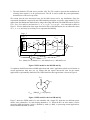
A GSPN consists of four primitive objects: places, activities, input gates and output gates. Figure 1
shows an example of a GSPN model.
2
O1
I1
T1
P1
P2
T3
T2
P3
Figure 1 An example GSPN model.
T4
Places: Circles in Figure 1 represent places. Each place may contain zero or more tokens, which represent
the marking of the place. The set of all place markings represents the marking of the system, M. M also
represents the state of the system. Only the number of tokens in a place matters. In Figure 1, the system
marking can be written as {P1+P2}, which means that there are one token in P1 and one in P2.
The meaning of the marking of a place is arbitrary. For example, the number of tokens in a place could
represent the number of requests awaiting service in one application and a request with a certain priority
level in another application. This flexibility in the meaning of a marking increases the expressiveness of
the GSPN for modeling a wide variety of dynamical systems.
Activities: Activities represent actions that take some amount of time to complete. There are two types of
activities: stochastic timed with an exponential distribution and instantaneous. Hallow ovals in Figure 1
represent timed activities. Timed activities have durations that impact the performance of the modeled
system. In GSPN, the duration of an activity is always an exponential distribution whose mean value
represents the average duration of that activity. The inverse of the mean value is called the transition rate
of that activity. The transition rate of an activity may be different depending on system markings.
Instantaneous activities represent actions that are completed in a negligible amount of time compared to
the other activities in the system. Solid vertical lines in Figure 1 represent instantaneous activities.
Case probabilities, represented in Figure 1 by small circles on the right side of an activity, model the
uncertainty associated with the completion of an activity. Each case stands for a possible outcome.
Definition A.1 A place is called a vanishing place if it is the only input place of an instantaneous activity;
otherwise the place is called a tangible place.
Input gate: Input gates enable/disable activities and define the marking changes that will occur when an
activity is completed. In Figure 1, triangles that point to the activity they control represent the input gates
(i.e., I1). There exist arcs from the places upon which the input gate depends (also called input places) to
the base of the triangle. Input gates are annotated with an enabling predicate and a function. The
enabling predicate is a Boolean function that controls whether the connected activity is enabled or not. It
can be any function of the markings of the input places. The function defines the marking changes to the
input places that will occur when the activity is completed. If a place is directly connected to an activity
such as P2 and T3 in Figure 1, this is the same as an input gate with a predicate that enables the activity if
there is at least one token in the input place and a function that decrements the marking of the input place.
Output gate: Similar to input gates, output gates define the marking changes that will occur when an
activity is completed. The difference is that output gates are associated with a case. In Figure 1, triangles
whose base is connected to an activity or a case represent output gates (i.e., O1). The triangles point to
arcs that connect to the places affected by the marking changes. Output gates are defined only with a
function. The function defines the marking changes that will occur when the activity is completed. If an
activity is directly connected to a place, this is the same as an output gate with a function that increments
the marking of the place.
3
For notational convenience, we will use the following notation: place names start with “P”, activity
names start with “T”, input gate names start with “I”, and output gate names start with “O.”
2.2
Executing GSPN
GSPN execution refers to the enabling of activities, completion of activities, and token movement (i.e.,
changes of system marking).
Activity enabling: An activity is enabled at a certain system marking M when the enabling predicates of
all the input gates connected to it are true and there is at least one token in each place that is directly
connected to it. In Figure 1, activities T2 and T3 are enabled in system marking M={P1+P2} because for
each of them, there is only one input place that contains one token. Activity T4 is not enabled in M
because there is no token in P3. The enabling predicate of I1 decides the enabling of T1.
Activity completion: An instantaneous activity is completed immediately after it is enabled. A timed
activity is completed if it is enabled for its duration time. Every time a timed activity is enabled, the
duration time is obtained by a random sample of the exponential distribution associated with this activity.
When a timed activity is enabled but not yet completed, the system marking may be changed by the
completion of another activity. If the activity has not enabled the new system marking, the completion of
that activity will not happen, and all information related to its previous enabling will be disregarded in the
future.
Marking change: Change of system marking is only evaluated when there is an activity completion.
When an activity is completed, one of its cases (notice that there may be only one case for the activity) is
chosen based on the pre-defined case probability. Then the following steps are taken: all of the directly
connected input places have their markings (i.e., number of tokens) decremented; the input places
connected through input gates change their markings according to the input gate functions; all of the
places directly connected to the selected case have their markings incremented; the places connected
through output gates change their markings according to the output gate functions.
Definition: The reachability set of a GSPN from an initial marking M0, denoted as RS(M0), is the set of
all possible system markings that can be achieved as a result of a sequence of activity completions.
2.3
Controllable GSPN with cost
Definition: A GSPN with cost is a GSPN model with two types of cost: impulse cost associate with
marking transitions and rate cost associated with system markings. Impulse cost occurs when the GSPN
makes a transition from one marking to another. Rate cost is the cost per unit time when the GSPN stays
in a certain marking.
Definition: A controllable GSPN is a GSPN where all or part of the case probabilities of activities can be
controlled by external commands.
2.4
Distributed Multimedia System
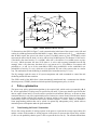
Figure 2 shows a simplified view of a distributed MM system with QoS management [17]. The system
consists of three components: an MM server with a database of multimedia objects and a database of QoS
information, the transport system that mainly consists of a network of communication channels, routers
and switches, and the MM client, which can be a portable personal computer, pocket PC or another
mobile multimedia devices.
4
MM Server
MM Database
QoS Database
MM Client
MM data
MM data
Resources: CPU,
memory, etc.
Local QoS manager
Local QoS manager
Transport System
Resources: Network
Local QoS manager
Global QoS manager
Figure 2 QoS managed, distributed multimedia system.
Each component has its own local QoS manager. The global QoS manager controls the QoS negotiation
and renegotiation procedure among the components. The procedure can be briefly described as follows.
The local QoS manager reports the available local resources to the QoS manager. The global manager
computes the QoS that each component needs to deliver based on the available resources and sends the
requirement to the local manager. The local manager uses its available resources to enforce the local QoS
requirement and keeps on monitoring the local QoS. If there is a local QoS violation, the local manager
sends a request to the global manager, who will respond to the request by either re-allocating the local
QoS requirement among the different components or negotiating with the user to adopt a degraded global
QoS.
Because low power design is targeted at electronic components with limited power source, we focus on
PQ management for the MM client. The assumption being that the MM client has a large (or infinite)
power source. In this context, the “local QoS manager” of the MM client in Figure 2 will be referred to as
the “local PQ manager.”
3
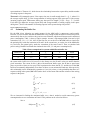
Modeling the PQ-Managed Client
Only components related to the PQ management problem are shown in this block diagram. Although the
GSPN formalism can model complex systems with multiple, interacting service providers, in this paper,
we use a simple system with a single service provider. This is because the focus of this paper is on power
and QoS management, not on complex system modeling. As an example of using GSPN to model a
complex power-managed system with multiple interacting service providers, please refer to [14].
Figure 3 gives a simplified block diagram of our PQ-managed client.
5
MM Buffer
MM Stream
Service
Provider
Local application
Scheduling
Control
Power Mode
Control
Request Queue
QoS constraints
Local PQ Manager
Figure 3 Block diagram of a PQ-managed MM client.
As shown in Figure 3, the MM client consists of a service provider (SP) that may be a CPU, a DSP or an
array of hard disks. The SP provides services (e.g., computing, processing, communication, data retrieval
and storage) for service requests coming from applications running on the MM client. We divide the
applications into two categories: the MM applications and the “other” applications. We separate the MM
applications because of their distinguishing features as explained below:
1. The distribution of request inter-arrival times is non-exponential, which requires special treatment
during the modeling process;
2. The QoS requirement is only applicable to the MM application;
3. The priority of the service requests from the MM application is usually higher than those from
“other” applications.
MM application
SR
SQ
TS
Other application
SR
SP
SQ
Figure 4 Top-level GSPN model for the MM client.
Figure 4 shows the top level GSPN model for the MM client. It is divided into three major parts:
1. MM service requester (SR) and service queue (SQ): The MM SR is used to model the statistical
behavior of the input MM stream, and the MM SQ is used to model the behavior of the MM buffer.
The GSPN model is shown in Figure 5.
2. Local SR and SQ: These are used to model the behavior of request generation and as a buffer for
other applications. The GSPN model is shown in Figure 6.
6
3. The task scheduler (TS) and service provider (SP): The TS is used to represent the mechanism for
selecting what request (is to be processed next. The SP is used to model the power/performance
characteristics of the service provider.
We assume that the unit inter-arrival time for the MM stream can be any distribution. Since the
exponential distribution is required by the GSPN modeling technique, we use the “stage method” [14] to
approximate the MM stream distribution by using a three-stage SR model. The MM SR consists of places
PMMa, PMMb, PMM1 and PMM2 and activities µ1, µ2, µ3, α1 (β 1 = 1-α1), α2 (β 2 = 1-α2) connected as shown in
Figure 5. Given a distribution of the input inter-arrival time of the MM stream, we can obtain the values
of µ1, µ2, µ3, α1 and α2 by curve fitting. PMMBuf represents the MM SQ.
Stage_3
Stage_2
Stage_1
µ1
PMMa
β1
PMM1
µ2
PMMb
β2
PMM2
µ3
α2
PMMBuf
α1
GMM: {Mark(PMM1)+Mark(PMM2) = 0 & Mark(PMMBuf) < MM buffer size
Figure 5 GSPN model for the MM SR and SQ.
To emphasize the difference between MM applications and “other” applications (which we will denote as
normal applications from now on), we assume that the request inter-arrival time for the normal
applications is exponentially distributed. The GSPN model for these applications is shown in Figure 6.
Tnorm
PSQ
Gnorm: { Mark(PSQ) < SQ capacity
Figure 6 GSPN model for the local SR and SQ.
Figure 7 shows the GSPN model of a task scheduler and a simple SP, which has two different power
modes: active (denoted as “a”) and sleeping (denoted as “s”). When the SP is in active mode, it can be
processing MM applications, which is denoted by mode (a, MM), or processing normal applications,
which is denoted by mode (a, norm).
7
Ts2a
Ta2s
Pa2s
Tdecision(s)
Pdecision(s)
Tdecision(a)
Ps2a
Pdecision(a)
Pidle(a,MM)
Pidle(s)
Pwork(a,MM)
Tprocess(a,MM)
Tstart
PMMBuf
Tredecision
Tvanish
Pchanging
Pidle(a,norm)
Pwork(a,norm)
Tprocess(a,norm)
PSQ
Figure 7 GSPN model for the SP and TS.
To illustrate how the GSPN in Figure 7 works, assume that the initial state of the system is active-idle and
waiting for a MM application and the MM buffer is empty. When a token arrives at PMMBuf, which means
that an MM request has arrived, the token in place Pidle(a,MM) moves to place Pwork(a,MM), which
represents the state of the SP when it is active and servicing an MM request. The duration t of this service
is decided by the timed activity Tprocess(a,MM). After time t, the token in Pwork(a,MM) moves to place
Pdecision(a), which represents the state of SP when it is active and accepting command from the PQ
manager. After a very short time, the token in Pdecision(a) moves to Pa2s, Pidle(a,MM) or Pidle(a,norm) with
probability a1, a2 and 1-a1-a2. In the controllable GSPN, these probabilities are the controllable case
probabilities of activity Tdecision(a), which are to be optimized. The rest of the system works in a similar
way. The mechanism of task scheduling is modeled by the immediate activity Tdecision(a).
The PQ manager reads the states of all system components and sends commands to control the task
scheduling and the SP state transition.
The GSPN model of the MM client is then automatically transformed into a continuous-time Markov
decision process (CTMDP), based on which the optimal PQ management policy is solved.
4
Policy optimization
The input to our policy optimization algorithm is the required QoS, which can be represented by (D, J,
L). In real applications, D (delay) may be specified in time units; J (jitter) may then be specified in time
units or square of time units; L (loss rate) may be specified in real numbers. However, we do not use these
constraints directly in our policy optimization process. Instead, we convert D and J from the time domain
to an integer domain related to the number of requests waiting in the queue. Next we remove the L
constraint by buffer size estimation based on the relation between L, D and J. Finally we formulate a
linear programming problem that can be solved for optimal PQ management policy, which achieves
minimum power consumption under the QoS constraints.
4.1
Transforming the D and J Constraints
We use the average number of waiting requests in the queue to represent the average request delay (D)
and the variance of the number of waiting requests in the queue to represent the request delay variance
(J). We use the probability that the queue is full to represent the loss rate (L). The rationale behind these
8
representations is Theorem 4.1, which shows the relationship between the request delay and the number
of waiting requests in the queue.
Theorem In a PQ-managed system, if the request loss rate is small enough, then D = Q ⋅ λ, where D is
the average request delay, Q is the average number of waiting requests in the queue and λ is the average
incoming request speed. Furthermore, during any time period of length T, ET(d) = ET(q) ⋅ T / X, where
ET(d) and ET(q) denote the average request delay and average number of waiting requests in the queue
during time T, and X is the number of incoming requests in this system during time period T.
Proof: (omitted to save space).
4.2
Estimating the Buffer Size
For the MM client, allocating too much memory for the MM buffer is unnecessary and wasteful.
However, we have to make sure that the MM buffer is big enough so that the SP does not need to provide
unnecessarily fast service to achieve the given loss rate constraint, which would in turn result in undesired
power consumption. Table 1 shows a simple example. Assume a PQ-managed MM client and a QoS
constraint of (D, J, L) = (1.5, 0.9, 0.02). In the first case, we set the size of the MM buffer to 4 and solve
the optimal policy under the constraints of D and J. In the second case, we set the size of the MM buffer
to 6 and solve the optimal policy under the constraints of the same D and J. Then we simulate both
policies using UltraSAN and obtain the simulated value of D, J, L and power consumption (P).
Table 1 Power comparison for systems with different buffer size
Buffer size
4
6
D
1.23
1.5
J
0.75
0.9
L
0.02
0.02
Power
2.08
1.49
From the above table we can see that the system with a buffer size of 4 consumes 40% more power than
the system with a buffer size of 6; however, in the former case, the D and J values are smaller than the
given constraints. The reason for this is that, with insufficient buffer space, the SP has to spend extra
power to provide a faster service speed. This experiment also shows that D, J, L and the size of the MM
buffer are not mutually independent. Given three of them, we can estimate the fourth one. More precisely,
their relationship can be formulated by equations (4.1) to (4.4), where pi is the probability that there are i
requests waiting in the queue (MM buffer) and m and v are the mean value and the variance of the waiting
requests in the queue.
n
∑ i ⋅ pi
i =1
=m
n
∑ (i − m) 2 ⋅ p n
i =0
n
∑ pi
i =0
(4.1)
=v
(4.2)
=1
(4.3)
0 ≤ pi ≤ 1, i=1, …, n
.
(4.4)
We are interested in finding the minimum buffer size n that is needed to avoid unnecessary power
consumption due to over constraints on D and J. This problem can be solved as follows:
Min. n
n
Subject to: ∑ i ⋅ p i = D ,
(4.5)
i =1
9
n
∑ (i − m) 2 ⋅ p n
i =0
n
∑ pi
i =0
=J,
(4.6)
= 1,
(4.7)
(4.8)
pn ≤ L ,
(4.9)
0 ≤ pi ≤ 1, i=1, …, n
We cannot solve above problem exactly. However, after some simplification, we find that if n satisfies
inequality relations (4.10)-(4.12), there will be a set of pi, which satisfies function (4.5) – (4.9).
(n - 2)2 ⋅ L ≥ J + D2 – 4 ⋅ D + 3,
(4.10)
(n + 1) ⋅ (n – 2) ⋅ L ≥ m – 2,
(4.11)
(n − 2) ⋅ (n – 1) ⋅ L ≥ D2 – 3 ⋅ D + 2 + J
(4.12)
Therefore, we obtain an upper bound on the minimum required buffer size:
Nup = Max(n1, n2, n3)
(4.13)
where n1, n2, n3 are the solutions of equations (4.10), (4.11) and (4.12). If the allocated buffer size is
larger than Nup, there will not be extra power waste due to over-constraining D and J. Note that this buffer
size estimation is independent of the incoming-data rate and the system service rate, because we assume
that the given QoS constraint (D, J, L) can always be satisfied by the optimal policy.
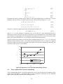
We have performed experiments to verify our buffer estimation method, we set J = 1.5, L = 5%. By using
different D values between 1 and 3.5, we estimate the minimum buffer size, Nup, using (4.13). Figure 8
shows the comparison between the estimated value and the real value that is obtained by simulation. The
results show the correctness of our method.
12
10
8
N
6
4
real value
estimated value
2
0
0.5
1.5
2.5
3.5
D
Figure 8 Comparison of real value and estimated upper bound.
4.3
Policy optimization by Linear Programming
The PQ management problem is to find the optimal policy (set of state-action pairs) such that the average
system power dissipation is minimized subject to the performance constraints for the traditional
application and the QoS constraints for the MM application.
10
First we give the definition of some variables. The reader may refer to [14] regarding how to calculate
some of the variables from a given CTMDP model.
a
piji : Probability that the next system state is j if the system is currently in state i and action ai is
taken.
τ iai :
a
xi i :
Expected duration of the time that the system will be in state i if action ai is chosen in this state
Probability that the next state of the system will be i and action ai will be taken if a random
observation of the system is taken
powi: System power consumption in state i
q_MMBufi: Number of unprocessed data in MM buffer
eneij: Energy needed for the system to switch from state i to state j
Ai: Set of available actions in state i
Our LP problem is formulated as follows:
LP1:
Min
∑i ∑ai xi i ( powi ⋅τ i i + ∑ j eneiji
a
a
{ xi i }
subject to
a
a
∑ai xi i − ∑ j ∑ ai x j i ⋅ p jii
a
a
∑i ∑ai xi i τ i i
a
a
xi i ≥ 0
a
a
a
⋅ p iji )
(4.14)
= 0 i∈S
=1
all i, ai
a
∑i ∑ai xi i
a
⋅ q _ MMBuf i ⋅ τ i i < D
∑i ∑ai xi i ⋅ (q _ MMBuf i − D) 2 ⋅τ i i
a
a
<J
(4.15)
Equation (4.15) gives the constraint on jitter, which is represented by the jitter of q_MMBufi. Note that the
left hand side of (4.15) does not give the exact jitter of q_MMBufi, which is:
∑i ∑ a i x i i
a
⋅ ( q _ MMBuf i −
∑ i ∑ ai x i i
a
a
a
⋅ q _ MMBuf i ⋅τ i i ) 2 ⋅ τ i i
(4.16)
Equation (4.16) contains nonlinear terms. For computational efficiency, we opted to use an approximation
of jitter so that the resulting mathematical program remains linear.
a
Proposition: For any set of {xi i } , that satisfies (4.15), the value of (4.16) is less than J.
Proof:
To
∑ i ∑ ai x i i
a
a
a
∑i ∑ ai xi i ⋅ (q _ MMBuf i − m) ⋅τ i i ,
minimize
a
⋅ q _ MMBuf i ⋅τ i i .
Therefore,∀m,
(4.16)
we
gives
know
the
that:
smallest
m
=
value.
■
From the above proposition we know that for any policy, if it satisfies constraint (4.15), then the real jitter
of q_MMBufi using this policy is less than constraint J. Hence we can use (4.15) instead of (4.16).
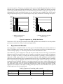
Figure 9 shows an illustration of q_MMBufi distribution when the system is using the PQ-optimized
policy and the PD-optimized policy (which in previous work, optimizes power only under delay
constraint). In this example, we set the MM buffer size to 8. The average length of the MM buffer is the
11
same for both policies. The power consumption of the system using the PD-optimized policy is 25% less
than that of the system using the PQ-optimized policy. However, the q_MMBufi jitter and loss rate of the
system using the PD-optimized policy are 3X and 1000X larger than those of the system using the PQoptimized policy. In the experimental results, we can achieve the same q_MMBufi jitter for the system
using PD-optimized policy by over-constraining the average delay and therefore consuming more power.
0.4
0.35
0.3
0.25
0.5
0.4
0.3
0.2
0.15
0.1
0.05
0
0.2
0.1
0
0 1 2 3 4 5 6 7 8
0 1 2 3 4 5 6 7 8
q_MMBufi distribution using
PQ-optimized policy
q_MMBufi distribution using PDoptimized policy
Figure 9 Comparison of q_MMBufi distribution.
Notice that in LP1, only the QoS constraint for the MM application was included. We can easily add the
performance constraint (i.e. delay) for the normal applications.
5
Experimental Results
Our target system is a simplified model of a client system in distributed MM system. System details are as
follows. The SR has only a request generation state. The average inter-arrival time of a traditional request
is 50ms. The SQ capacity is 3. The average inter-arrival time of the MM data is 20ms.
The SP has two p_modes: high-power mode and low-power mode. It takes 0.2J energy to switch from
high-power mode to low-power mode and 0.5J energy to switch from low-power mode to high-power
mode. To simplify the model, we assume that the time needed for switching is small enough to be
neglected. In both power modes, the SP can process both the MM applications and the normal
applications, but with different power consumption and speed. There is also another scenario in which the
SP is not processing any application. In this case, the service speed of SP is 0, and only a very small
amount of power is consumed. Therefore, in our target system, there are three a_modes: MM, normal and
idle. Table 2 and Table 3 give the SP power consumption and average service time in each combination
of p_mode and a_mode. Here, we assume that the high-power mode is designed specifically for MM
application. For example, in this mode a floating-point co-processor is used so that the service speed of
the MM application increases significantly.
Table 2 SP power (w) in each (p_mode, a_mode)
High power
Low power
MM
4
2
Normal
3
1.5
12
Idle
2
1
Table 3 SP service speed (ms) in each (p_mode, a_mode)
MM
5
10
High power
Low power
Normal
2
2.5
Idle
0
0
Table 4 Comparison between PQ-optimized and PD-optimized policies
QoS
Constraints
(1, 1, 0.1%)
(1, 1.5, 0.1%)
(3, 1, 0.1%)
(3, 1.5, 0.1%)
(5, 1, 0.1%)
(5, 1.5, 0.1%)
PD-optimized
Powe D
J
r
2.15 0.55 0.96
1.75 0.80 1.46
2.15 0.55 0.96
1.75 0.80 1.46
2.15 0.55 0.96
1.75 0.80 1.46
PQ-optimized
Powe D
J
r
1.95 0.86 0.98
1.63 1.00 1.49
1.92 2.86 0.98
1.57 2.93 1.50
1.72 4.80 0.97
1.47 3.69 1.46
∆P
(%)
9.3
6.9
10.7
10.3
20.0
16.0
In our experiment, because the normal application is not time critical, we set the performance constraint
of normal application simply as loss rate ≤ 5%. We use different QoS constraints (D, J, L) for the linear
programming problem. We solve LP1 to find the PQ-optimized policy. We use the procedure in [14] to
find the PD-optimized policy under the given D constraint. If the resulting jitter and loss rate cannot meet
the QoS constraints, we decrease D and recalculate the PD-optimized policy until they meet the
constraints. The results are shown in Table 4.
From the above results, we reach the following conclusions:
1. Our method can calculate the PQ-optimized policy for the MM client for given QoS constraints by
solving the LP problem only once while the previous DPM method has to obtain the PD-optimized
policy for given QoS constraints by solving the LP problem multiple times.
2. Our method can obtain the PQ-optimized policy that matches the given QoS constraints while the
previous method can only meet the QoS constraints by over-constraining the delay requirement,
which results in larger power consumption.
6
Conclusions
We have presented a new modeling and optimization technique for Power and QoS management in
distributed multimedia systems. QoS in this context refers to the combination of the average service time
(delay), the service time variation (jitter) and the network loss rate. We model the power managed
multimedia system with guaranteed QoS as a GSPN and the PQ-optimal policy is obtained by solving a
linear programming problem. Because jitter and loss rate are correlated parameters, we could not include
both of them into the LP formulation directly. Instead we removed the loss rate constraint from the LP
formulation by estimating the maximum size of the queue that stores the MM data. Furthermore, the jitter
constraint is a non-linear function of the variables we wanted to optimize. Therefore it could not be
directly used in the LP formulation. We were able to substitute the original jitter constraint with another
linear constraint, which we mathematically proved to be correct.
Previous methods only consider the delay constraint while obtaining the PD-optimized policy. They can
only meet the jitter and loss rate constraints by over constraining the delay. Compared to these methods,
we show that our PQM method can achieve an average of 12% more power saving.
13
REFERENCES
[1] A. Chandrakasan, R. Brodersen, Low Power Digital CMOS Design, Kluwer Academic Publishers, July 1995.
[2] M. Horowitz, T. Indermaur, and R. Gonzalez, “Low-Power Digital Design”, IEEE Symposium on Low Power
Electronics, pp.8-11, 1994.
[3] A. Chandrakasan, V. Gutnik, and T. Xanthopoulos, “Data Driven Signal Processing: An Approach for Energy
Efficient Computing”, 1996 International Symposium on Low Power Electronics and Design, pp. 347-352,
Aug. 1996.
[4] J. Rabaey and M. Pedram, Low Power Design Methodologies, Kluwer Academic Publishers, 1996
[5] L. Benini and G. De Micheli, Dynamic Power Management: Design Techniques and CAD Tools, Kluwer
Academic Publishers, 1997.
[6] M. Srivastava, A. Chandrakasan. R. Brodersen, “Predictive system shutdown and other architectural
techniques for energy efficient programmable computation," IEEE Transactions on VLSI Systems, Vol. 4, No.
1 (1996), pages 42-55.
[7] C.-H. Hwang and A. Wu, “A Predictive System Shutdown Method for Energy Saving of Event-Driven
Computation,” Proc. of the Intl. Conference on Computer Aided Design, pages 28-32, November 1997.
[8] G. A. Paleologo, L. Benini, et.al, “Policy Optimization for Dynamic Power Management”, Proceedings of
Design Automation Conference, pp.182-187, Jun. 1998.
[9] Q. Qiu, M. Pedram, “Dynamic Power Management Based on Continuous-Time Markov Decision Processes”,
Proceedings of the Design Automation Conference, pp. 555-561, Jun. 1999.
[10] Q. Qiu, Q. Wu, M. Pedram, “Stochastic Modeling of a Power-Managed System: Construction and
Optimization”, Proceedings of the International Symposium on Low Power Electronics and Design, 1999.
[11] L. Benini, A. Bogliolo, S. Cavallucci, B. Ricco, “Monitoring System Activity For OS-Directed Dynamic
Power Management”, Proceedings of International Symposium of Low Power Electronics and Design
Conference, pp. 185-190, Aug. 1998.
[12] E. Chung, L. Benini and G. De Micheli, “Dynamic Power Management for Non-Stationary Service Requests”,
Proceedings of DATE, pp. 77-81, 1999.
[13] L. Benini, R. Hodgson, P. Siegel, “System-level Estimation And Optimization”, Proceedings of International
Symposium of Low Power Electronics and Design Conference, pp. 173-178, Aug. 1998.
[14] Q. Qiu, Q. Wu, M. Pedram, “Dynamic Power Management of Complex Systems Using Generalized Stochastic
Petri Nets”, Proceedings of the Design Automation Conference, pp. 352-356, Jun. 2000.
[15] The QoS Forum, “Frequently Asked
http://www.qosforum.com/docs/faq/, 2000.
Questions
about
IP
Quality
of
Service”,
URL:
[16] A. Vogel, B. Kerhervé, G. V. Bochmann, J. Gecsei, “Distributed Multimedia and QoS: A Survey”, IEEE
Multimedia, pp. 10-19, Summur 1995.
[17] A. Hafid, G. V. Bochmann, “Quality of Service Adaptation in Distributed Multimedia Application”,
Multimedia System Journal, (ACM), Vol 6, No. 5, pp. 299-315, 1998.
[18] R. G. Herrtwich, “The Role of Performance, Scheduling, and Resource Reservation in Multimedia Systems”,
Operating Systems of the 90s and Beyond, pp, 279-284, A. Karshmer and J. Nehmer, eds. Sprintger-Verlag,
Berlin, 1991.
[19] M. A. Marsan, G. Balbo, G. Conte, S. Donatelli and G. Franceschinis, Modeling With Generalized Stochastic
Petri Nets, John Wiley & Sons, New York, 1995.
[20] UltraSAN User’s Manual, Version 3.0, Center for Reliable and high-Performance Computing, Coordinated
Science Laboratory, University of Illinois.
14