Download Axel Jacobs

Axel Jacobs
Radiance Tutorial
2
CONTENTS
Contents
1 Introduction
1.1 What is Radiance? . . . . . . . . . . . . . . . . . . . . . . . . . . . . . .
1.2 Ray-tracing vs. Radiosity . . . . . . . . . . . . . . . . . . . . . . . . . .
1.3 Do it the UNIX Way . . . . . . . . . . . . . . . . . . . . . . . . . . . . .
2 Describing a Scene in Radiance
2.1 General Information and Syntax . . . . . . . . . . .
2.2 Describing the Geometry . . . . . . . . . . . . . . .
2.2.1 Approaches to Modelling . . . . . . . . . . .
2.2.2 Modelling Geometry . . . . . . . . . . . . . .
2.2.3 More Complex Scenes . . . . . . . . . . . . .
2.3 Describing the Materials . . . . . . . . . . . . . . . .
2.3.1 Standard Materials . . . . . . . . . . . . . . .
2.3.2 Materials Modified by Patterns and Textures
2.3.3 Light Sources . . . . . . . . . . . . . . . . . .
2.3.4 Daylight . . . . . . . . . . . . . . . . . . . . .
.
.
.
.
.
.
.
.
.
.
.
.
.
.
.
.
.
.
.
.
.
.
.
.
.
.
.
.
.
.
.
.
.
.
.
.
.
.
.
.
.
.
.
.
.
.
.
.
.
.
.
.
.
.
.
.
.
.
.
.
.
.
.
.
.
.
.
.
.
.
.
.
.
.
.
.
.
.
.
.
.
.
.
.
.
.
.
.
.
.
.
.
.
.
.
.
.
.
.
.
8
8
8
9
.
.
.
.
.
.
.
.
.
.
10
10
12
12
13
15
18
18
19
20
21
3 Previews, Visualisation and Image Conversion
3.1 Quick Preview of Objects . . . . . . . . . . . .
3.1.1 objline . . . . . . . . . . . . . . . . . .
3.1.2 objpict . . . . . . . . . . . . . . . . . .
3.2 Visualisation . . . . . . . . . . . . . . . . . . .
3.2.1 Interactive Visualisation . . . . . . . . .
3.2.2 Non-interactive Visualisation . . . . . .
3.3 Image Conversion . . . . . . . . . . . . . . . . .
.
.
.
.
.
.
.
.
.
.
.
.
.
.
.
.
.
.
.
.
.
.
.
.
.
.
.
.
.
.
.
.
.
.
.
.
.
.
.
.
.
.
.
.
.
.
.
.
.
.
.
.
.
.
.
.
.
.
.
.
.
.
.
.
.
.
.
.
.
.
.
.
.
.
.
.
.
.
.
.
.
.
.
.
.
.
.
.
.
.
.
.
.
.
.
.
.
.
23
23
23
23
24
24
25
25
4 How Radiance Works
4.1 Ambient Calculations . . . . . . . . . . .
4.2 Ambient Parameters . . . . . . . . . . . .
4.2.1 Useful Ranges . . . . . . . . . . . .
4.2.2 Artifacts Associated with Options
4.2.3 Timings Associated with Options .
.
.
.
.
.
.
.
.
.
.
.
.
.
.
.
.
.
.
.
.
.
.
.
.
.
.
.
.
.
.
.
.
.
.
.
.
.
.
.
.
.
.
.
.
.
.
.
.
.
.
.
.
.
.
.
.
.
.
.
.
.
.
.
.
.
.
.
.
.
.
28
28
32
32
32
33
.
.
.
.
.
.
34
34
34
35
36
36
37
Joy of Rendering
Too Much to Remember . . . . . . . . . . . . . . . . . . . . . . . . . . .
The rad command . . . . . . . . . . . . . . . . . . . . . . . . . . . . . .
Being Lazy . . . . . . . . . . . . . . . . . . . . . . . . . . . . . . . . . .
41
41
41
42
5 Analysing Scenes
5.1 Analysing Radiance pictures . . . . . . .
5.1.1 Creating False Colour Images . .
5.1.2 Analysis With ximage . . . . . .
5.2 Analysing Models with rtrace . . . . .
5.2.1 Getting an Illuminance Reading
5.2.2 Plotting Illuminance Values . . .
6 The
6.1
6.2
6.3
References
.
.
.
.
.
.
.
.
.
.
.
.
.
.
.
.
.
.
.
.
.
.
.
.
.
.
.
.
.
.
.
.
.
.
.
.
.
.
.
.
.
.
.
.
.
.
.
.
.
.
.
.
.
.
.
.
.
.
.
.
.
.
.
.
.
.
.
.
.
.
.
.
.
.
.
.
.
.
.
.
.
.
.
.
.
.
.
.
.
.
.
.
.
.
.
.
.
.
.
.
.
.
.
.
.
.
.
.
.
.
.
.
.
.
.
.
.
43
3
Axel Jacobs
Radiance Tutorial
A Appendices
A.1 The Main Primitives and Their Parameters . . . .
A.1.1 Materials . . . . . . . . . . . . . . . . . . .
A.1.2 Surfaces . . . . . . . . . . . . . . . . . . . .
A.2 Suggested File Name Extensions . . . . . . . . . .
A.3 Suggested Project Directory Structure . . . . . . .
A.4 Files Used in the Course . . . . . . . . . . . . . . .
A.5 Material files for the pattern and texture example .
A.5.1 wood.mat . . . . . . . . . . . . . . . . . . .
A.5.2 wood pat.cal . . . . . . . . . . . . . . . . . .
A.5.3 water.mat . . . . . . . . . . . . . . . . . . .
A.5.4 wrinkle.cal . . . . . . . . . . . . . . . . . .
A.6 File Listings . . . . . . . . . . . . . . . . . . . . . .
A.6.1 objects/chair.rad . . . . . . . . . . . . . . .
A.6.2 objects/table.rad . . . . . . . . . . . . . . .
A.6.3 materials/course.mat . . . . . . . . . . . .
A.6.4 skies/sky.rad . . . . . . . . . . . . . . . . .
A.6.5 lux.plt . . . . . . . . . . . . . . . . . . . . .
4
.
.
.
.
.
.
.
.
.
.
.
.
.
.
.
.
.
.
.
.
.
.
.
.
.
.
.
.
.
.
.
.
.
.
.
.
.
.
.
.
.
.
.
.
.
.
.
.
.
.
.
.
.
.
.
.
.
.
.
.
.
.
.
.
.
.
.
.
.
.
.
.
.
.
.
.
.
.
.
.
.
.
.
.
.
.
.
.
.
.
.
.
.
.
.
.
.
.
.
.
.
.
.
.
.
.
.
.
.
.
.
.
.
.
.
.
.
.
.
.
.
.
.
.
.
.
.
.
.
.
.
.
.
.
.
.
.
.
.
.
.
.
.
.
.
.
.
.
.
.
.
.
.
.
.
.
.
.
.
.
.
.
.
.
.
.
.
.
.
.
.
.
.
.
.
.
.
.
.
.
.
.
.
.
.
.
.
.
.
.
.
.
.
.
.
.
.
.
.
.
.
.
.
.
44
44
44
44
45
46
47
47
47
47
48
48
49
49
50
50
51
52
CONTENTS
Revision History
23 Jan 2012
• Fixed minor inconsistencies
• Reflect changes in Radiance 4.1, Dec 2011 (rpict -w) and Radiance HEAD, Jan
2012 (falsecolor)
19 Dec 2010
• Fixed a few inconsistencies
2 Apr 2010
• Moved section ’Secondary Light Sources’ to the Cookbook. I haven’t found the
time to cover it for about five years;
• Derived a simplified formula for the transmissivity in Appendix A.1.1, but put
all the explanations in the Cookbook.
• Some tidying up
25 Oct 2008
• Decided to eat my own dog food and be consistend with the recommended file
structure and naming conventions as laid out in A.3
• Some tidying-up
26 May 2008
•
•
•
•
Added suggested directory structure for projects to the appendix
Fixed a type with the transmittance formula in the appendid and added a graph
Moved the Introduction to UNIX to a separate document.
Change tables to the more formal tabular formatting, newly introduced in LYX
1.5
• Unified the hand-made bibliographies to BibTEX
• Added info on gamma correction to image conversion
26 Dec 2006
• Changed the section dealing with illuminance plots so that the measurement
points are read in from a file, and not generated by cnt. Many students find the
use of rcalc too confusing, and it’s not necessary here. The old cnt|rcalc version
is now in the Advanced Tutorial.
• Updated the falsecolor pages.
• New section on wild cards
• Added index
• Updated CAD import and primitives sections
• Added margin icons for files in the ZIP archive
10 Nov 2006
• Added nicer front page and page headers
5
Axel Jacobs
Radiance Tutorial
• Put all images into floats and gave them captions
• Added reference to Colour Picker on LUXAL
• Corrected a few typos here and there
6 June 2006
• More explanation on using rcalc in 5.2.
18 Feb 2005
• Added 4.2 Ambient Parameters which is essentially copied from rpict.options
• Added rule of thumb for setting an appropriate -av (based on exposure)
• Increased font size to 11pt for better readability
19 Dec 2004
•
•
•
•
Added this revision history
Added chapter 3: Previews, Visualisation and Image Conversion
Changed all reference from rview to rvu
Included examples for textures and patterns in 2.1 General Information and Syntax
• Updated the listing of the ambient default settings for rvu in 4.1 Ambient Calculations to reflect the new settings in Radiance 3.6
• Scrambled author’s email addresses on front page to block email harvesters
6
CONTENTS
About the Use of Fonts
Several different fonts are used throughout this document to improve its readability:
typewriter: commands, file listings, command lines, console output
italics: paths and file names
sans serif : Radiance primitives, modifiers, identifiers
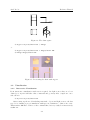
Suggested Reading
There are number of different Radiance study guides and tutorials available with
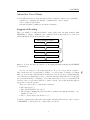
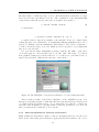
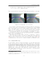
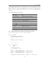
LEARNIX [3]. Figure 1 illustrates the optimal work flow that will give you the best
understanding in the shortest amount of time.
UNIX for Radiance, Chapter 1
UNIX for Radiance, Chapter 2
Difficulty
Radiance Tutorial
Radiance Cookbook
Understanding rtcontrib
Figure 1: You are strongly encouraged to follow this path while studying the LEARNIX
documentation.
You are encouraged to follow this suggestion. If you do feel proficient enough to
skip certain sections of a particular document, or even an entire document, you might
miss out on some important information that later sections rely upon. Simply skipping
over parts that you might find boring or otherwise un-interesting will leave serious gaps
in your understanding of Radiance. It is important that you try to understand all
exercises, and you absolutely MUST do them yourself. Don’t just flick through the
pages and look at the pictures.
There are other sources of information, namely:
• The man pages [6],
• The official Radiance web site [7],
• The Radiance mailing list and its archives, available through the Radiance community web site [10],
• The book Rendering with Radiance [9].
You may consult them at any time, either while studying with the help of the resources
on LEARNIX, or afterwards. Good luck with your efforts.
7
Axel Jacobs
1
1.1
Radiance Tutorial
Introduction
What is Radiance?
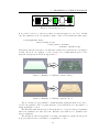
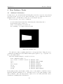
Radiance is a sophisticated lighting visualisation system. Originally started off as a
research project at the Lawrence Berkeley Laboratories, it has evolved into an extremely
powerful package that is capable of producing physically correct results and images that
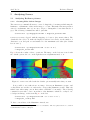
are indistinguishable from real photographs.
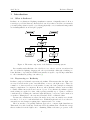
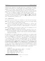
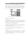
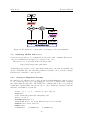
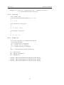
Figure 2: The main components of the Radiance rendering system
Its versatility makes Radiance the ideal choice not only for ’serious’ researchers but
also for architects, lighting designers and other professionals. Although a challenge to
learn, Radiance, especially in a UNIX environment, is capable of producing results that
no other visualisation package can achieve.[9]
1.2
Ray-tracing vs. Radiosity
Radiance employs backward ray-tracing algorithms. This means that the light ’rays’
are traced back from the point of measurement or view to the light source. There are
a number of other ray-tracers on the market because the basic principle is relatively
simple to implement on computers. However, where Radiance stands out is its ability
to handle diffuse inter-reflections between objects. Very efficient algorithms together
with caching are applied for this. Other packages usually try to equate for indirect
contributions by defining the ’ambient’ light that has no real source and somehow is
everywhere. Examples for other ray-tracers include POV or 3DStudio Max.
Because the calculations are started from the view point, an entirely new calculation has to be done for each individual view. Walk-throughs and videos are therefore
extremely resource-hungry requiring fast computers and a lot of time.
There is another conceptually different approach to compute light distributions.
This method is called radiosity. Radiosity-based algorithms start off with the energy
that is radiated from the light source. Assuming diffuse reflectance properties of the
8
1
INTRODUCTION
objects, the incoming energy is then modified by the material’s reflective properties
and bounced back into the room. This is done until the contribution of the reflected
light towards the average illuminance in the scene becomes insignificant.
The energy distribution of the entire scene is calculated and stored. This means
that once all the calculations are done, new view points can be created in no time at
all. This makes the radiosity solutions ideal for the creation of virtual worlds such as
VRML. Scenes created this way can usually be told because of their lack of reflective
and transparent surfaces, although newer software implements get-arounds to these
problems. A typical example of a simulation package that uses radiosity is VIZ (ex
Lightscape) by AutoDesk.
1.3
Do it the UNIX Way
The Radiance source code is freely available for download from the Internet. Radiance
was developed to run on UNIX machines. Part of the reason is that in the early
1990s when Greg Ward started writing Radiance, computers were very slow compared
to today’s machines. It did not make sense to run processing intensive applications
such as ray-tracers on desktop PCs. Most ’serious’ workstations, operated under UNIX
which provides a multitasking environment.
It is the UNIX philosophy to have very modular software. This is in stark contrast
to the concept that MS Windows and the Mac OS follow. They aim to provide GUIbased software packages that do everything the average user could possibly ask for and
a lot more. The drawback with this is that the software can only do what its designers
had in mind when they programmed it.
Radiance in contrast consists of more than 100 individual programs. This makes it
extremely flexible. By defining options and chaining together two or more programs, a
maximum flexibility can be achieved. Unfortunately, it also means that a steep learning
curve is the price to pay.
Please refer to the separate UNIX for Radiance document for an introduction to
UNIX and use of the command line [5]. It is essential that you study Chapter 1 of
that document before proceeding further!
9
Axel Jacobs
2
Radiance Tutorial
Describing a Scene in Radiance
2.1
General Information and Syntax
Radiance uses a Cartesian (rectilinear) coordinate system. All information is stored in
ASCII text format, so it can be edited with any text editor. Please refer to appendix
A.2 for some commonly used file name extensions.
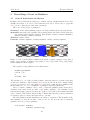
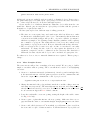
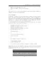
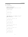
There are 4 basic types of primitives:
Geometry: source, sphere (bubble), polygon, cone (cup), cylinder (tube), ring, mesh, instance
Materials: light, illum, glow, spotlight, mirror, prism1, prism2, mist, plastic, metal, trans, plastic2, metal2, trans2, dielectric, interface, glass, plasfunc, metfunc, transfunc, BRTDfunc,
plasdata, metadata, transdata, antimatter
Textures: texfunc, texdata
Patterns: colorfunc, brightfunc, colordata, brightdata, colorpict, colortext, brighttext
Figure 3: Some of the Radiance primitives (from left to right): a polygon of type glass, a
sphere of type dielectric, a cylinder of type plastic, a cone of type metal, a ring of type plastic
with a brightfunc texture applied
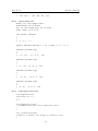
The syntax for any primitive follows this scheme:
modifier type identifier
n S1 S2 ... Sn
0
m R1 R2 ... Rm
The type has to be one of the predefined surface, material, pattern or texture types that
are known to Radiance. The identifier can be freely chosen but should be unique within
your project. Please refer to Appendix A.1 for the most commonly used primitives and
their parameters, or to [8] for a full list of primitives and their parameters.
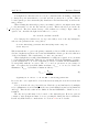
Before a surface primitive can be used, a material primitive must exists whose
identifier is the same as the modifier of the surface primitive. By chaining several
material and texture/pattern descriptions together, very detailed and realistic materials
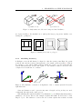
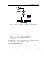
can be defined. This chain is shown in Fig 4. While material and geometry primitives
are always required, textures and patterns are optional.
The first primitive in this chain has no modifier, so void is used. The identifier of the
first primitive becomes the modifier of the second one. We need at least one material
primitive and one geometry primitive:
void plastic chairmat
chairmat cylinder leg1
10
2
DESCRIBING A SCENE IN RADIANCE
Figure 4: Describing an object
It is possible, however, to have more than one material applied to an object. In this
case, the primitives are hooked up like a chain, connected by identifier-modifier pairs:
void brightfunc dusty
dusty texfunc woody
woody plastic chairmat
chairmat cylinder leg1
Patterns modify the reflectance of a material, textures are perturbations of a surfaces
normal. Below is one example of each, described by a mathematical model. The
material descriptions are listed in Appendix A.5.
Figure 5: Example of a Radiance texture: Water
Figure 6: Example of a Radiance pattern: Wood
The second line in every primitive contains all string arguments that are needed to
describe the primitive. The very first character (’n’) is an indicator for the number of
string arguments to follow.
The third line must always read 0. It was intended to be used for integer arguments
when new primitives are introduced into Radiance but until now no primitive uses
integer arguments.
The last line holds real arguments or floating point numbers. Again, the integer in
front (’m’) indicates the total number of arguments to follow.
11
Axel Jacobs
Radiance Tutorial
Comments are preceded by a hash sign (’#’) and proceed to the end of the line. If
the first character in a line is an exclamation mark (’!’), then this is taken as a shell
command. The line is executed and the result of this command returned.
2.2
2.2.1
Describing the Geometry
Approaches to Modelling
All Radiance scene files are stored as plain text. This allows us to edit them with any
text editor. It is thus possible to build up a model by simply deciding which geometry
primitives to use, and supplying the required coordinates, dimensions etc.
To aid in the creation of such hand-build models, Radiance comes with a number
of helper programs that are commonly referred to as generators. You can get a list of
available generators by running the following command in your terminal:
$ ls /usr/bin/gen*
genblinds
genbox
genclock
genprism
genrev
gensky
gensurf
genworm
In this tutorial, we will be using the genbox command to create a simple rectangular
room, as well as gensky which defines the distribution of certain CIE-defined standard
skies.
The complexity of hand-generated models is limited. You will find that generating
the scene geometry with a CAD or 3D modelling package is more convenient and faster.
Converters are available that allow us to export from a limited number of commonly
used 3D file formats to Radiance. Such converters might be plug-ins to the relevant
software package as is the case with the su2rad plug-in for Sketchup [12]. Others are
command-line applications. Examples include converters for the 3DS, OBJ and DXF
formats
If you decide to use a CAD package for doing the modelling, you should be aware
that objects can be modelled in different ways. A box, for instance, may be modelled
as:
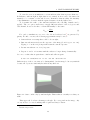
1. The six surfaces if the box. This is a surface model.
2. The volume contained by the box. A solid model.
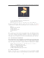
Only surface models are suited for use in Radiance. See Fig 7. A well-written
translator might be able to convert volume models into surface models, because all
the necessary information is contained within the model. When in doubt consult the
documentation of your CAD software.
Most CAD modellers will only export objects of type polygon. This is fine. Polygons
are by far the most frequently used type of geometry. Just be aware that once a polygon
is defined, you can’t later cut a hole in it, e.g. to put in a window. If this is what you
need to do, there are several options to your disposal. Some obvious and useful ones
12
2
DESCRIBING A SCENE IN RADIANCE
(a) Surface model
(b) Solid model
Figure 7: Only surface models can be imported into Radiance.
are depicted in Fig 8. It’s usually best to split up the larger polygon into smaller ones,
leaving the opening free.
Figure 8: Cutting a hole into a polygon
2.2.2
Modelling Geometry
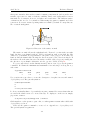
A Radiance scene should always be aligned so that the x-axis points East, the y-axis
points North, and the z-axis points upwards to the zenith, as shown in Fig 9. This is
in contrast to some 3D modelling packages which use x and y for the horizontal and
vertical dimensions and describe the depth. i.e. the distance behind or in front of the
computer screen with the z coordinate.
Figure 9: The Radiance convention on alignment of the coordiante system follows the
right-hand rule
Sizes and distances can be given in any unit of length, as long as they are used
consistently throughout the entire project.
When flicking through the Radiance User Manual [8], you will find that many surface
primitives come in two flavors. An example is sphere and bubble. Both describe a ballshaped object. The difference between the two is that a sphere has a surface normal
13
Axel Jacobs
Radiance Tutorial
that point outwards, whereas the normal of a bubble points inwards. As long as the -bv+
switch to rpict is set to turn on back-face visibility, this doesn’t really matter for most
materials. It does matter, however, for light sources and mirror. The different surface
orientations also need to be remembered when using the genbox command and other
generators. It creates outward pointing surfaces normals by default. To swap this, use
the -i switch with genbox.
Figure 10: Direction of the surface normal
The surface normal follows the right-hand rule. Form a loose fist with your right
hand but have your thumb stick up. Hold your hand in such a way that the axis
defined by your thumb is perpendicular to the plane of the polygon. Now turn your
hand around the thumb-axis following the direction given by the other four fingers. If
the indices follow the same direction, the surface normal of the polygon is pointing into
the direction of your thumb. Otherwise, it’s the opposite. Please see Fig 10.
To get a rough idea about the dimensions and position of an object, use the getbbox
command. It returns the minimum and maximum of an enclosing box along the x, y
and z axis.
$ getbbox chair.rad
xmin
xmax
0
0.5
ymin
0
ymax
0.5
zmin
0
zmax
1
Use your favorite text editor to create the description of a sphere in a new file named
objects/things.rad. The general syntax is:
modifier sphere identifier
0
0
4 xcent ycent zcent radius
Look at your first Radiance object with the objline command. It creates what is known
as a meta file which can not be viewed directly. To display it on the screen, simply
pipe it into x11meta.
$ objline objects/things.rad | x11meta
Click anywhere on the picture to quit. Also, see what getbbox returns when called with
objects/things.rad now.
Next, use the genbox command to create a box. Append it to objects/things.rad.
The general syntax for genbox is:
14
2
DESCRIBING A SCENE IN RADIANCE
genbox material name xsize ysize zsize
Additional options are available, such as rounded or chamfered edges. Please refer to
the genbox man page for details. Open objects/things.rad in a text editor and remove
two or three adjacent faces. Look at the result with objline.
Create another box of different dimensions. This time, don’t call it from the command line. Instead, put an extra line in objects/things.rad that calls the generator.
Remember to begin the line with ’ !’.
We have just explored two different ways of calling generators:
• The first one creates quite large and cumbersome files but allows us to make
modifications to individual parts of the object. Unfortunately, this is what most
converters from CAD packages will produce. A perfect cylinder, for instance,
which is very simple to model using a native Radiance primitive, will be split up
into a number of polygons. The result will not look not very nice, unless a very
large number of polygons is created. However, this will result in large file sizes.
• The second way is nice because it is only one line of text that we can easily
understand. To change the size of the box only requires the alteration of one
argument, compared to twelve coordinates done the other way. The drawback of
this method is that only the whole object can be modified, not just parts of it.
For what we’ve done so far, no material definitions were required. This is going to
change.
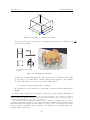
2.2.3
More Complex Scenes
The next exercise will produce something a bit more useful. We are going to build a
simple room with a window opening. The room will then be used for our daylighting
excercises.
1. Create a room that is 4.0 m wide (x-dimension), 5.0 m deep and 3.0 m high. Give
it the material wall mat. Call the genbox generator from the command line and
direct the output of the command into a file objects/room.rad :
$ genbox wall_mat room 4 5 3 > objects/room.rad
2. Change the material of the polygons that form the floor and the ceiling to floor mat
and ceiling mat respectively. The materials wall mat, floor mat, and ceiling mat are
already defined in materials/course.mat. You’ll find the listings of most files used
in our exercises in Appendix A.6 of this document.
3. Lower the south wall to create an opening, setting the height of the wall to 1.0 m.
See Fig 11 for help.
4. Create a pane of glass that fits into the new opening. Make sure there are no
gaps and that the entire room remains airtight. Assign glazing mat as a modifier.
5. Create a file called furniture.rad 1 from which you call xform to place a table in
the scene and a couple of chairs around it. You’ll find them in objects/table.rad
15
Axel Jacobs
Radiance Tutorial
(4.0, 5.0, 3.0)
3.0 m
z
5.0 m
x
y
4.0 m
Figure 11: A simple room with an opening
and objects/chair.rad , respectively. Use getbbox and objline to see whether you
get the desired result.
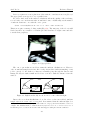
(a) A chair viewed with
objline
(b) Four chairs around the table
Figure 12: Arranging the furniture.
objline is somewhat unusual in the sense that is produces X11 meta files. This
is a special vector format that looks like garbage when output to the terminal.
To render the image, we need to pipe it into x11meta like so:
$ objline objects/chair.rad | x11meta
We will later on meet another program that works in tandem with x11meta:
bgraph.
6. Create a file objects/bulb.rad 2 which describes the geometry and the material for
1
You would be right in saying that furniture.rad should sit in the objects/ subdirectory. Unfortunately, objline and objview don’t parse nested in-line calls to xform the same way, and it is safer if
furniture.rad remains in the root of our project directory.
2
You shouldn’t really call this thing a ’bulb’. In the vocabulary of a lighting engineer, a bulb is
something you plant in your garden. A ’lamp’ is the thing inside a ’luminaire’ that generates the light
which the luminaire shapes and models. An example for a ’lamp’ would be a tungsten halogen reflector
lamp, an example for a luminaire could be that thing on your desk that looks very stylish, throws really
bad light, and has a lamp inside.
16
2
DESCRIBING A SCENE IN RADIANCE
the light bulb. Place the sphere at the origin of the coordinate system and give
it a radius of 3.0 cm. For now, we assume a white light source. Use the material
light and give it equal values for the red, green, and blue radiance. Please refer to
section 2.3.3 for more information on coloured lamps.
7. In a file called lights.rad, us xform commands to place two of your bulbs at a
height between 2.5 and 3.0 m.
Before we catch a first glimpse of the image, the scene needs to be compiled into an
octree. The purpose of an octree is to speed up the calculation by only considering the
objects that lay within the path of a ray. The command to use is oconv. It takes as
arguments all material and scene files that we want to include. oconv will not compile a
scene file unless all materials that are used are defined. To make things easier, the file
materials/course.mat contains everything that is needed in this exercise. The materials
have to be given first, or oconv will drop out with an error. The octree is produced at
STDOUT, so you will need to redirect it into a file.
$ oconv materials/course.mat objects/room.rad \
objects/furniture.rad objects/lights.rad > scene.oct
There are three commands that accept an octree as an input and trace rays within the
scene. They all start with ’r’:
rvu for in interactive preview3 ,
rpict for producing an image, and
rtrace to trace a single ray.
Use rvu for an interactive view of the scene using the view parameters stored in the file
views/nice.vf.
$ rvu -vf views/nice.vf scene.oct
Figure 13: Our first interactive view
Once the rvu window is up, there are a number of interactive commands to adjust
parameters and views. You will probably have to adjust the exposure of the image
before you can see all the details correctly. The most commonly used commands are
listed below. They may be typed in full, or called by the first letter, e.g e for exposure.
3
prior to Radiance version 3.6, rvu used to be called rview.
17
Axel Jacobs
Radiance Tutorial
Command
Explanation
aim
Zoom
exposure
Set the exposure
frame
Set frame for refinement
last
Restore the previous view
new
Redraw display
pivot
Pivot view about selected point
quit
Quit
rotate
Rotate the camera
set
Change program variable
trace
Trace a ray
view
Change view parameters
write
Write picture file
Please look up the exact syntax and more detailed explanation in the rvu man page.
Another very hand little program is objview. It calls rvu for an interactive preview
of one or more objects. The difference between the two is that rvu will only work on
octrees, i.e. compiled scenes, whereas objview takes material (.mat) and geometry files
(.rad ) as inputs, so the compilation is unnecessary. Additionally, objview will put light
sources into the scene, so objects can be looked at without putting a sky or luminaires
into the scene.
$ objview materials/course.mat objects/chair.rad
2.3
2.3.1
Describing the Materials
Standard Materials
A total of 25 different materials are available to describe the characteristics of the
surfaces. They range from the simple to use plastic or metal to the more complex ones
like dielectric and BRTDfunc which allow for the most accurate (and difficult) use, but
has settings for all directional aspects of reflectance and transmittance. Please refer to
[8] for a complete list, as well as detailed descriptions. Some further details can also be
found in Appendix A.1.1 of this document.
The material used for the majority of cases is plastic which defines a surface that
does not alter the colour of the highlights, i.e. highlights appear in the colour of the
light source rather than the colour of the material. This is true for most materials
around us, be it wood, paper, concrete, plastic or fabric.
Those are the arguments that the plastic primitive expects:
modifier plastic identifier
0
0
5 redrefl greenrefl bluerefl spec rough
18
2
DESCRIBING A SCENE IN RADIANCE
All values must be within the range of [0...1]. Most materials in reality have a roughness below 0.2 and a specularity below 0.1. The contribution of the individual RGB
components towards the average reflectance is weighted and equates to:
ρ = 0.265R + 0.670G + 0.065B
(1)
ρ = (0.265R + 0.670G + 0.065B) × (1 − S) + S
(2)
for metal and to
for plastic, with S being the specularity of the material. Don’t get confused when
reading through old documentation. You might find differing multipliers there. As of
version 2.5, Radiance uses the multipliers found in Eqn 1. The reason for this has to
do with cones in the retina of our eyes, which are more responsive to green light than
they are for red and blue.
Use your favorite image manipulation package such the The GIMP to pick a nice
colour and apply it to the seat and back of our office chair. The range of colours in
most graphics packages is between 0 and 255. So you’ll need to scale this down to a
range between 0 and 1. What is the reflectance of the fabric?
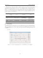
Figure 14: The JALOXA colour picker is a handy tool for specifying materials
There is quite a useful colour picker for Radiance on the JALOXA web site. You
may use it for picking a plastic or metal material by moving the interactive sliders across
[4]. With its help it’s much easier to choose materials, as it will also compute the
reflectance and normalised colour (important for sky and ground) for you. You can
just copy-and-past the results into your *.mat file.
2.3.2
Materials Modified by Patterns and Textures
While defining the materials for plain colours is a straight-forward process, the scene
will look more interesting and real when we apply patterns and textures to the object.
19
Axel Jacobs
Radiance Tutorial
Patterns describe changes in colour, while textures refer to perturbations of the surface
normal. A picture mapped onto a frame hanging on the wall is an example for a pattern.
Ripples on a body of water, on the other hand, can be created through textures.
We can string as many patterns and textures together as we like, the sky is the
limit. How about a dusty wooden table with stains and a chess board laid in and some
scribble on it? A combination of brightfunc, colorpic and texfunc will do the trick.
materials/course.mat has two brightfunc and one colorfunc primitives defined for you.
Create a nice blue stripe across the walls by applying blue band to wall mat. Additionally,
use floorpat to put some random tiles on the floor and make them look dirty with dirt.
Try to understand what each function does.
2.3.3
Light Sources
The available materials for light sources in Radiance are: light, illum, glow and spotlight.
light is the basic material for self-luminous surfaces. It is used for most light emitting
objects. It’s used to model the sun in a clear sky.
illum is used for secondary light sources with broad distribution, i.e. windows. illum
sources are treated like ordinary light sources except when looked at directly.
They then act as if they were made of a different material. See section ?? for
details.
glow is for self-luminous surfaces that have a limited effect. For daylighting, it is used
for the sky hemisphere, as well as for the ground.
spotlight is used for light sources with a directional output. It has little relevance, since
it gives rather unrealistic results. For ’real’ spot lights, it’s much preferrable to
use the light material in combination with a data file describing the luminance
distribution of the fitting.
For physically correct results, it is important to determine the correct radiance values
for the red, green, and blue channel. The lampcolor program does this for us. We
use the type WHITE here. Use this whenever you are rendering a scene that is only
lit by one type of light source, irrespective of what this may be. A mechanism called
’colour adaptiation’ causes our brains to automatically adjust to the colour temperature
of the predominant light source in a scene. This is similar to the auto-whitebalance
function that is built into digital cameras. Choosing a none-white lamp type is only
recommended if there are different types of lamps in a scene, e.g. metal halides and
tungsten. If you assign a WHITE (i.e. non-coloured) lamp type to all your light sources,
you can colour-balance the white point of the final rendering with the pfilt command
at a later stage. A list of available lamp types can be found in lamp.tab. On our
LEARNIX system, this file resides under /usr/share/radiance 4 . A normal tungsten
lamp has a luminous efficacy of around 15 lm/W. We assume a 100 W lamp.
$ lampcolor
Program to compute lamp radiance. Enter ’?’ for help.
Enter lamp type [WHITE]: incandescent
Enter length unit [meter]: meter
Enter lamp geometry [polygon]: sphere
Sphere radius [1]: .03
4
If you have compiled Radiance yourself, it will be in /usr/local/lib/ray
20
2
DESCRIBING A SCENE IN RADIANCE
Enter total lamp lumens [0]: 1500
Lamp color (RGB) = 235.85 235.85 235.85
^C
These values need to be given as real arguments to the material primitive defining the
material of the bulb. Use the material light.
2.3.4
Daylight
Descriptions of daylight are generated with the gensky command. It defines the distritbution of sky and ground radiance. It is left to the user to define two hemispheres of
type source—one for the sky, the other for the ground. source objects are infinitely far
away from any observer and defined by their direction and an angle, rather than their
absolute x, y, z coordinates, as all other Radiance geometry primitives are. It is also
left to he user to take care of the colours of sky and ground.
To start with, let’s create a sunny sky for London at today’s date. You should
redirect the output to a file called skies/sky.mat.
$
#
#
#
#
gensky 12 09 14:00 -a 51 -o 0 -m 0
gensky 12 09 14:00 -a 51 -o 0 -m 0
Local solar time: 14.14
Solar altitude and azimuth: 11.0 29.9
Ground ambient level: 8.7
void light solar
0
0
3 2.72e+06 2.72e+06 2.72e+06
solar source sun
0
0
4 -0.489041 -0.851114 0.190903 0.5
void brightfunc skyfunc
2 skybr skybright.cal
0
7 1 3.76e+00 3.72e+00 2.98e-01 -0.489041 -0.851114 0.190903
gensky will only create the distribution of sky and ground as well as the material
definition and the actual object for the sun. Materials for sky and ground and the two
hemispheres are left to the user to define.
Sun
Sky
Distribution
-
gensky > skies/sky.mat
Material
gensky > skies/sky.mat
user > skies/sky.rad
Geometry
gensky > skies/sky.mat
user > skies/sky.rad
21
Axel Jacobs
Radiance Tutorial
You might notice that the table above is not consistent with our naming conventions
to always keep the materials in a .mat file and the geometry in a .rad file. This is
because gensky produces materials (sky distribution and sun material), as well as the
sun geometry.
When defining the material properties, care must be taken to use skyfunc as modifier
to the material for both, the sky and the ground. This is already done in the file
skies/sky.rad . The photometric average of the radiances according to Eqn 3 must be
equal to 1.0, otherwise the light levels will not be correct.
1.0 = 0.265R + 0.670G + 0.065B
(3)
Now bring up the result in rvu. Set up a nice fisheye view of the sky hemisphere
and save the parameters into views/fish.vf.
$ oconv skies/sky_overcast.mat skies/sky.rad > sky.oct
$ rvu sky.oct
When run with the -c option, the gensky command produces a CIE overcast sky whose
absolute brightness and hence the horizontal illuminance that it produces is a function
of the solar altitude. The actual sun is, of course, not generated.
When daylight factors rather than illuminance readings are required, it is convenient
to work with a 10,000 lx sky. This way, we can simply divide the illuminance by 100 to
get the daylight factor. To create a sky that produces a certain horizontal illuminance,
we run gensky with the -B option. The -a, -o and -m options are not necessary for
this. -B requires the horizontal diffuse irradiance, Rhoriz , so we need to divide the
illuminance, Ehoriz , by Radiance’s luminous efficacy:
Rhoriz =
Ehoriz
179lm/W
(4)
$ gensky 12 4 +12:00 -c -B 55.866 > skies/sky_10klx.mat
Re-create the octree again and look at it interactively using the view file from the last
exercise.
Now look in the file skies/sky 10klx.mat. Find the ground ambient level, multiply
it by π (illuminance from a hemispherical source) and multiply again by 179 (luminous
efficacy). This should result in the diffuse horizontal illuminance, which we set to
10,000 lx.
The sky and ground must both be made of the material glow. However, glow, in
contrast to light, spotlight and illum, does not get sampled during the direct calculation.
It will only make indirect contributions. See section 4.1 for more details.
22
3
3
PREVIEWS, VISUALISATION AND IMAGE CONVERSION
Previews, Visualisation and Image Conversion
Radiance objects and scenes can be visualised with a number of different programs.
Except for objline, they are all based on either rvu or rpict, and add functionality or
convenience through scripts. The diagram in Fig 15 attempts to give an overview of
the viewers in Radiance and when they can be used. The programs on the right-hand
side are sorted in increasing complexity and image quality from top to bottom.
Figure 15: Different commands are available to view your scene
3.1
3.1.1
Quick Preview of Objects
objline
Whilst modelling the geometry of an object or scene, it is often useful to get a quick
overview of the size and position of objects. The objline program is useful for quickly
visualising the geometry without having to worry about correct material definitions.
The software produces the result in meta format which is vector rather than pixel-based.
To display it on the screen, please pipe it through x11meta.
$ objline objects/chair.rad | x11meta
Alternatively, an Encapsulated PostScript output can be produced which can then
be imported into other documents. The evince document viewer that is available on
LEARNIX can display the EPS format.
$ objline objects/chair.rad | psmeta > images/chair.eps
Don’t forget that there is also the getbbox command which will tell you how big the
object is and where it is located.
3.1.2
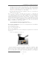
objpict
If all materials, as well as the geometry of the objects, are defined except for the light
sources, the objpict program can generate a four-view image of the objects by taking
care of placing some light sources in the scene to make sure the objects are actually
visible. The output is a Radiance image, so don’t forget to redirect the output into a
*.hdr file or pipe it into ximage:
23
Axel Jacobs
Radiance Tutorial
Figure 16: The chair again...
$ objpict objects/chair.rad | ximage
or
$ objpict objects/chair.rad > images/chair.hdr
$ ximage images/chair.hdr
Figure 17: Previewing the chair with objpict
3.2
3.2.1
Visualisation
Interactive Visualisation
If an interactive visualisation with rvu is required but light sources have not been
defined yet, objview will take a list of material and geometry files, compile an octree
and call rvu.
$ objview objects/chair.rad
After setting up the model including materials, objects and light sources, the last
step before running a proper simulation with rpict is oftentimes to define a nice view.
This is rather difficult to achieve on the command line, but very easily done interactively
within rvu.
24
3
PREVIEWS, VISUALISATION AND IMAGE CONVERSION
Figure 18: The chair in rvu
$ oconv skies/skyovercast.mat skies/sky.rad \
objects/chair.rad > chair.oct
$ rvu -vp 10 10 10 -vd -1 -1 -.98 -vh 5 -vv 5 -ab 1 chair.oct
On the rvu command line, adjust the exposure and save the image. For a list of
commands that are available in the rvu shell, please refer to the table in section 2.2.3.
done: e
Pick point for exposure
w chair_rvu.hdr
writing chair_rvu.hdr...
v views/chair.vf
done:
Once you have a good view, save the view parameters into a file. Make sure it has a
*.vf extension. This is not necessary for Radiance to pick it up, but makes it a lot
easier on you to remember what all those files in your directory are. That is also the
reason why you are encouraged to store all of your view files in the views/ directory.
3.2.2
Non-interactive Visualisation
After all these preparations, it’s finally time to hit the BIG button (not that this exists
on the command line...). Most commands in the next section assume that the image has
been given a good exposure that makes most of the objects visible within the dynamic
range of the display device (monitor or printer). This is done with the pfilt command.
$ rpict -vp 10 10 10 -vd -1 -1 -.98 -vh 5 -vv 5 -e .1 -ab 1 \
chair.oct > images/chair_rpict.hdr
$ pfilt -e .5 images/chair_rpict.hdr \
> images/chair_rpict_pfilt.hdr
$ ximage images/chair_rpict_pfilt.hdr &
3.3
Image Conversion
Radiance comes with tools for converting images from the special Radiance RGBE
format other formats. All such converters start with ra_* in their name, for example
25
Axel Jacobs
Radiance Tutorial
ra_tiff will convert the Radiance RGBE format to a TIFF. The TIFF format is un-
derstood by virtually all image processing software, but results in rather large file sizes.
It might therefore be a good idea to convert from TIFF to a file format which results
in smaller files. The PNG (pronounce “ping”) format is ideally suited for this.
Although ImageMagick is not part of the Radiance distribution, it is installed on
many UNIX and LINUX systems and also on LEARNIX. ImageMagick [1] provides a
number of programs for displaying and manipulating image files. The convert command
uses the file extension to decide what format to export to.
$
$
$
$
$
$
cd images
pfilt -e 1 chair_rpict.hdr > chair_rpict_pfilt.hdr
ra_tiff chair_rpict_pfilt.hdr chair_rpict_pfilt.tif
convert chair_rpict_pfilt.tif chair_rpict_pfilt.png
rm chair_rpict_pfilt.tif
cd ..
All of the above assumes that the Radiance image file has a proper exposure set using
the pfilt command. Run it without any options to automatically set a good exposure
without having to worry about the correct exposure multiplier. If the dynamic range
of the image is too high, the bright regions in the image will become washed out, while
subtle shades of dark grey turn into black.
It is possible to take the unfiltered image and compress the dynamic range so that
both dark and bright regions are visible. Radiance supplies the normtiff program for
this, which may also be used to mimic certain characteristics of the human visial system.
$ normtiff images/chair_rpict.hdr \
images/chair_rpict_normtiff.tif
$ convert images/chair_rpict_normtiff.tif \
images/chair_rpict_normtiff.png
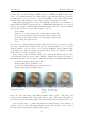
(a) 1.0: Default of Im- (b) 1.8: Used in printing (c) 2.2: Default for Ra- (d) 3.0: For comparison
ageMagick’s convert
diance’s normtiff and
ra_tiff. Used for CRT
monitors
Figure 19: The same image with different gamma values applied. The image was
prepared with normtiff rather than pfilt and ra_tiff. This ensures that there is
pure black and pure white in the image. The gamma value affects mostly the mid-tones.
It is very important to be aware that Radiance’s normtiff and ra_tiff default to a
gamma correction of 2.2, while ImageMagick’s convert has a default of 1.0. 19 shows
the same image with different gamma values applied.
26
3
PREVIEWS, VISUALISATION AND IMAGE CONVERSION
ImageMagick is one of the few packages that can read the Radiance image format
directly 5 . To convert a Radiance image file to PNG format, type
$ convert -gamma 2.2 images/chair_rpict_pfilt.hdr \
images/chair_rpict_pfilt.png
The PNG image format utilses a loss-less file compression which is perfect for reports
and similar documents where the overall document size is not important.
If you want to publish the images on the Internet, you want to make sure the file size
is as small as possible, in which case it is advisable to use the JPEG format instead.
JPEG images use a lossy compression which creates potentially much smaller files,
but might suffer from artifacts when high compression factors are used. Compression
factors below 50 will almost certainly exhibit such artifacts. A compression factor of
100, which is the maximum, will minimise such problems, but results in larger file sizes.
$ convert -gamma 2.2 -quality 80 \
images/chair_rpict_pfilt.hdr images/chair_rpict_pfilt.jpg
It is also possible to create GIF images, however, this format can only display a maximum of 255 colours. The PNG format does not have those disadvantages.
The mogrify program of ImageMagick allows for the quick conversion of multiple
images to a different format. Combined with a little shell magic, it is possible to convert
a large number of files in one go:
$ cd images
$ for file in *.hdr ; do normtiff $file \
$(basename $file hdr)tif ; done
$ mogrify -gamma 2.2 -format jpg *.tif
$ cd ..
to convert to TIFF using Radiance’s normtiff command and then to JPEG, or
$ mogrify -gamma 2.2 -format png images/*.hdr
to convert to PNG with ImageMagick’s mogrify.
5
convert actually relies on the Radiance ra_ppm to do the work
27
Axel Jacobs
4
4.1
Radiance Tutorial
How Radiance Works
Ambient Calculations
Compile a new octree and include the following files: materials/course.mat, skies/sky.mat,
skies/sky.rad and objects/room.rad. Give it the name scene.oct. Make sure there is no
furniture in the room and that you have an overcast sky in sky.mat.
We now view the octree scene.oct with rvu:
$ oconv materials/course.mat skies/sky.mat skies/sky.rad \
objects/room.rad > scene.oct
$ rvu -vf views/nice.vf scene.oct
rvu: warning - no light sources found
Figure 20: A black room
You will notice that everything inside the room appears black. Using the trace
command from within rvu, check whether this is just a question of poor exposure or if
the room really is black.
Check the default settings for -ab and -av for rvu.
$ rvu -defaults |grep ^-a
-av 0.000000 0.000000 0.000000
-aw 0
-ab 0
-aa 0.300000
-ar 32
-ad 256
-as 64
#
#
#
#
#
#
#
ambient
ambient
ambient
ambient
ambient
ambient
ambient
value
value weight
bounces
accuracy
resolution
divisions
super-samples
Both parameters have 0 as default. A value of zero for the number of ambient bounces
turns the ambient calculation off. So only light sources of type light, spotlight or illum
will be sampled. Since the sky is made of glow, it does not take part in the direct
calculations, resulting in the black interior.
28
4
HOW RADIANCE WORKS
To view the scene, it is sufficient to set an ambient value that is greater than zero.
In Radiance ambient light is light that is not emitted from a source but instead is
assumed to be constant over the whole scene. Remember that in reality, the intensity
of the illuminance decreases with the squared distance from the light source.
To determine the value of the ambient irradiance the following formula can be
applied. The -av option enables us to supply different values for the red, green, and
blue channel, however, the three of them will usually be the same.
Ramb =
Eamb
179π
(5)
For outdoor simulations, set -av to the Ground ambient level 6 as generated by
gensky. For indoor scenes, the following approximation may be used7 :
1. Start with an -av setting that could be about right;
2. Run rvu and interactively set the exposure of the image (don’t forget to set -ab).
Typing ’e =’ at the rvu prompt will return the current exposure.
3. Re-run rvu with an -av of 0.5/exposure.
4. Repeat 2. and 3. a few times until the values no longer change dramatically.
Set -av to a value that is equivalent to 500 lx and call rvu again.
$ rvu -vf views/nice.vf -w -av .89 .89 .89 scene.oct
Different faces of the room can now be distinguished, but the image looks very artificial
because all objects are uniformly lit without any shadows.
Figure 21: Our room lit only by ambient light. This is almost certainly not what you
want.
This approach does have advantages, though. For every pixel in the image, only
one ray needs to be traced making this a ’quick and dirty’ solution.
6
7
This value is in units of W/m2 .
Radiance Digest V3n2
29
Axel Jacobs
Radiance Tutorial
Before you quit rvu, create a plan view of the entire floor and save it as views/floor.vf.
The appropriate view type is ’l’ for a parallel view.
In order to find out how the indirect calculation affects the quality of the rendering,
set -av back to zero and run rvu with one ambient bounce. Additionally, set the number
of ambient divisions to one with the -ad 1 option.
$ rvu -vf views/floor.vf -av 0 0 0 -ab 1 -ad 1 scene.oct
This is now quite a strange looking result (Fig 22)8 . The majority of the floor is still
black, but there are a number of circular splotches that have a bright centre and fade
towards their periphery.
Figure 22: Ugly splotches
The -ab 1 option that we used here turns the ambient calculations on. However,
only one ambient sample ray is sent off for each position where ambient sampling occurs
(-ad 1 option). So the chances of this ray eventually going through the window and
hitting the sky are rather small and decrease even more with the distance from the
window.
−ab 0
−ab 1
Figure 23: Light from the sky needs one more bounce than sun light
But we also see a cheat that Radiance does. In order to reduce its workload, ambient
sample rays are not sent out for every pixel. It is assumed that the ambient light does
8
Update Nov. 2006: Creating this particular result is no longer possible under Radiance version 3.7
or higher. The minimum number of ambient division (-ad) is now set to 27, or 3 if -ab is set to zero. I
left this image here, because it shows rather well what happens during the ambient calculation.
30
4
HOW RADIANCE WORKS
not change a lot throughout the scene, which is usually correct. Every point for which
the ambient light did get sampled carries a ’sphere of influence’. As long as a new
pixel lies within a radius R of this sphere, a new ambient sampling is not carried out.
Instead, the values of adjacent sampling points are interpolated. The radius of the
’sphere of influence’ is:
maxSize × aa
(6)
ar
MaxSize is the maximum scene dimension as returned by getbbox, aa and ar refer the
settings for -aa and -ar which control the ambient accuracy and the ambient resolution,
resp.
Increase the ambient divisions to 64 and see what this results in. Does it look like
Fig 24?
Rmin =
Figure 24: The room with one ambient bounce
In order to make the scene look less patchy, two approaches can be taken:
• Greatly increase the setting for -ad
• Get Radiance to sample our window as if it was a ’real’ light source. This is done
with the mkillum command and is explained in the Radiance Cookbook [2].
Raphael Compagnon’s Radiance Course Notes [11] feature a table showing the minimum
number of sample rays needed to certainly hit a glow source that sustains a certain solid
angle. Here are examples taken from there:
Angular Resolution (o )
Required -ad
Required -ds
1
33863247
0.02
5
54446
0.09
10
3455
0.17
20
230
0.35
30
50
0.54
31
Axel Jacobs
Radiance Tutorial
It is clear that as the light source gets smaller, the number of ambient sample rays
required to hit the glow source explodes. For very small sources, this stochastic sampling
becomes too unreliable and computing intensive.
4.2
Ambient Parameters
The following tables are copied from the file rpict.options which is distrisbuted with
Radiance. Only ambient parameters are listed. Please refer to the original file for a
complete listing. The column labelled ’Very Accur’ is not from the original table but
was added because it gives you a better idea about appropriate options for accurate
daylighting simulations.
4.2.1
Useful Ranges
Parameter
Description
Min
Fast
Accur
Very Accur
Max
-ab
ambient bounces
0
0
2
5
8
-aa
ambient accuracy
0.5
0.2
0.15
0.08
0
-ar
ambient resolution
8
32
128
512
0
-ad
ambient divisions
0
32
512
2048
4096
-as
ambient super-samples
0
32
256
512
1024
min for fastest, crudest rendering. It is not necessarily the smallest value numerically.
fast for reasonably fast rendering.
accur for reasonably accurate rendering (artificial lighting)
very accur for accurate rendering or complicated scenes (daylighting)
max for the ultimate in accuracy.
Avoid using the “max” setting for -aa and -ar. This disables optimisation and can be
very expensive in terms of rendering time.
4.2.2
Artifacts Associated with Options
Parameter
Artifact
Solution
-ab
lighting in shadows too flat
increment value
-av
overall light level seems too high/low
decrease/increase value
-aa
uneven shading boundaries in shadows
decrease value by 25%
-ar
shading wrong in some areas
double or quadruple value
-ad
“splotches” of light
double value
-as
“splotches” of light
increase to half of -ad setting
32
4
4.2.3
HOW RADIANCE WORKS
Timings Associated with Options
Parameter
Effect on Execution Time
-ab
doubling this value can double rendering time
-aa
doubling this value approximately quadruples rendering time
-ar
effect depends on scene, can quadruple time for double value
-ad
doubling value may double rendering time
-as
effectively adds to -ad parameter and its cost
33
Axel Jacobs
5
Radiance Tutorial
Analysing Scenes
5.1
5.1.1
Analysing Radiance pictures
Creating False Colour Images
The falsecolor command allows us to create looking false colour images which map the
luminance or illuminance values in the image to colours. This makes the interpretation
easier for us humans, since we are more adept to distinguish colours than shades of
grey. The following command line will do just this:
$ falsecolor -ip imagegs/scene.hdr > images/fc_defaults.hdr
falsecolor creates a legend9 with the mapping of colours to photometric values. The
default label is cd/m2 . To make the displayed values a bit rounder, set the number of
divisions to ten, and pick a round number for the maximum scale value (the default
here is ’auto’):
$ falsecolor -ip images/scene.hdr -s 500 -n 10 \
> images/fc_better.hdr
Fig 25 shows the results of these operations: The image on the left was created with
the default options, the one on the right has some adjustments made to it.
(a) Default options
(b) Better scale and nicer legend
Figure 25: falsecolor called with the default options usually isn’t what you want
It is possible to use values from one image, let’s say an illuminance picture, and
overlay them onto another one, such as the corresponding luminance picture. This only
makes sense when using contour lines rather a full false colour image. The following
command creates false colour contour lines of the luminance which are overlayed onto
a background image, as shown in Fig 26 on the left:
$ falsecolor -ip images/scene.hdr -cl -s 500 -n 10 \
> images/fc_overlay.hdr
To have contour lines of the illuminance instead, use:
9
The default palette has changed in version 3.8 of Radiance. The new palette has more colours in
it, which makes it easier to interpret.
34
5
ANALYSING SCENES
$ falsecolor -i images/scene_i.hdr -p images/scene.hdr -cl \
-n 10 -s 2000 -l lux > images/false.hdr
The -l option sets the label of the legend10 . The result is shown in Fig 26 on the right.
(a) Luminance
(b) Illuminance
Figure 26: Producing false colour contour lines
If you’re still not entirely happy with the way that pixel values are represented by
falsecolor, please feel free to try out alternative colour palettes (-pal option). An HDR
image of the available palettes can be generated with the -palettes switch11 . Don’t
forget to pipe this to ximage, or to save it to a file. You may also want to experiment
with the -cb or -cp options that create contour bands or a posterisation effect, resp.
Understanding the difference between the illuminance and luminance, you will appreciate why the contour lines follow the carpet pattern in the false colour luminance
picture, but not in the illuminance one.
When using falsecolor with overlaid contour lines, you might have to adjust the
exposure of the background image. Do this before running pfilt. The image from
which the values are extracted never needs to have its exposure adjusted. Figs 27 and
28 summarise the use of the falsecolor command for luminance and illuminance scales.
5.1.2
Analysis With ximage
If only a handful of values are required from an image or if other values such as pixel
position or the ray direction are of interest, the ximage command can be of help. The L
key will display the luminance/illuminance value at that point on the screen. If ximage
was started from a command line, typing the T key or pressing the middle mouse button
will print out one or more of the following: Ray origin, ray direction, radiance value,
luminance value or pixel position. This output can be controlled with the -o option
when calling ximage. It can then be processed in a spread sheet or dealt with directly,
for instance with the rcalc command.
10
Until version 4.1 of Radiance (Dec 2011), this had a default of ’nits’, which is the same as ’cd/m2’.
It now defaults to ’cd/m2’.
11
This and the -cp option have been available in Radiance HEAD since Jan 2012, and will be released
in Radiance proper with version 4.2
35
Axel Jacobs
Radiance Tutorial
Figure 27: Flowchart for creating false colour images of the pixel luminance
5.2
Analysing Models with rtrace
rtrace traces rays given to it on STDIN and produces the result on STDOUT. Like the two
other r*-commands (rvu and rpict), it operates on an octree.
The rays need to be specified in the following format:
xorg yorig zorig xdir ydir zdir
Technically, it is possible to create entire images with rtrace. Because it is usually only
used for individual rays, the rendering parameters default to more accurate settings.
Check rtrace -defaults to find out more.
5.2.1
Getting an Illuminance Reading
In a first step, we will use rtrace to find out the horizontal illuminance that is created
by our overcast sky. Since we’re only passing the one ray, we do this from the command
line rather than through a file. The UNIX echo command will do the job–it sends its
arguments to STDOUT. Make sure the file sky.oct only contains the description and the
material of a 10,000 lx overcast sky.
$ echo ’0 0 0 0 0 1’ | rtrace -I -ab 1 sky.oct
#?Radiance
oconv skies/sky_10klx.mat skies/sky.rad
rtrace -I -ab 1
SOFTWARE= Radiance 3.8
lastmod Sun Nov 11 17:10:54 GMT 2007 by root on birdie
CAPDATE= 2007:12:15 08:52:17
FORMAT=ascii
5.594485e+01
5.594485e+01
5.594485e+01
36
5
ANALYSING SCENES
Figure 28: Flowchart for creating false colour images of the pixel illuminance
The first eight lines of the output are the header which can be disabled with the -h
option to rvu12 :
$ echo ’0 0 0 0 0 1’ | rtrace -I -h -ab 1 sky.oct
5.591661e+01 5.591661e+01 5.591661e+01
Since sky.oct contains the description of a non-coloured grey sky, all three colour channels have the same value of 5.587436e+01, or 55.87 W/m2 . This is an irradiance reading.
If the sky was non-grey, we’d have to compute the average, weighted irradiance.
To get the illuminance, we simply multiply with the luminous efficacy of 179 lm/W:
$ echo ’0 0 0 0 0 1’ | rtrace -I -ab 1 -h sky.oct \
| rcalc -e ’$1=179*(.265*$1+.670*$2+.065*$3)’
10006.6961
The result is 10,000 lx. This is no surprise to us, because the sky was created with the
-b option to produce a horizontal illuminance of 10,000 lx.
5.2.2
Plotting Illuminance Values
This exercise is based on the previous one and uses the bgraph command to plot a graph
of lux levels at working plane height against the distance from the window. The height
of the working plane is usually taken to be 0.85 m. Fig 29 illustrates the task at hand.
The readings are spaced 0.5 m, with the first and last reading being no closer to
the walls than 0.5 m. Since the room is 5.0 m deep, that’s nine points in total. The
direction is up, or +z, to get the horizontal illuminance. A file called data/line.pts has
12
Before Radiance version 4.1 (Dec 2011), rtrace and rpict would issue a warning if the sky was
without sun and if the number of ambient bounces -ab was set to zero. Such warnings can be disabled
with the -w switch. This should no longer be necessary if you know what you’re doing.
37
Axel Jacobs
Radiance Tutorial
Figure 29: Taking illuminance readings
already been prepared for you. It lists the points of the measurement and the direction
vectors as (x,y,z) triplets:
$ cat data/line.pts
2.0 0.5 0.85 0 0 1
2.0 1.0 0.85 0 0 1
2.0 1.5 0.85 0 0 1
2.0 2.0 0.85 0 0 1
2.0 2.5 0.85 0 0 1
2.0 3.0 0.85 0 0 1
2.0 3.5 0.85 0 0 1
2.0 4.0 0.85 0 0 1
2.0 4.5 0.85 0 0 1
You can easily see that only the y-coordinate differs between the points. If you are
interested in how such a grid file can be created with Radiance’s rcalc command, please
refer to the chapter titled ’Dynamic grids with cnt’ in the Radiance CookbookAxel
Jacobs [2].
The points are now fed into rtrace:
$ cat data/line.pts | rtrace -I -ab 3 -h scene.oct
#?Radiance
oconv materials/course.mat skies/sky.mat \
skies/sky.rad objects/room.rad
rtrace
SOFTWARE= Radiance 3.7
lastmod Sat Nov 18 23:28:38 WET 2006 by ...
FORMAT=ascii
6.0374e+00
3.8192e+00
1.3492e+00
7.3870e+00
4.6729e+00
1.6508e+00
8.5235e+00
5.3918e+00
1.9047e+00
38
5
ANALYSING SCENES
...
rtrace will normally only output the value which is in our case the irradiance for the
Red, Green, and Blue channel. If run without the -I switch, this would be the radiance
instead. This is fine, except that plotting is easier if the position of the sensor is printed
as well the reading. This is done with the -o option: The default is -ov which prints
the values. Over-writing this with -oov will output the position, too. While we are
fiddling with the command-line options, we also need to get rid of the header (-h).
$ cat data/line.pts | rtrace -I
2.00e+00
5.0e-01
1.85e+00
2.00e+00
1.0e+00
1.85e+00
2.00e+00
1.5e+00
1.85e+00
...
-ab 3 -h -oov scene.oct
6.037e+00
7.387e+00
8.524e+00
3.819e+00
4.673e+00
5.392e+00
1.349e+00
1.651e+00
1.905e+00
To get the reading in lux rather than red, green, and blue irradiance values, Eqn (3)
has to help us out once more.
$ cat data/line.pts | rtrace -I -ab 3 -h -oov scene.oct \
| rcalc -e ’$1=$2;$2=179*(.265*$4+.670*$5+.065*$6)’ \
> results/lux.csv
$ cat results/lux.csv
0.5
1271.4789
1
804.313407
1.5
284.135595
2
477.732247
2.5
463.546922
3
405.675942
3.5
387.179138
4
431.251321
4.5
158.74665
Prepared for you is a file named lux.plt which gives some instructions to the bgraph
command. Modify it as you like. To output to the screen and to a PostScript file, resp,
use the following two command lines:
$ bgraph lux.plt | x11meta
$ bgraph lux.plt | psmeta > results/graph.eps
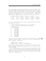
The plot in Fig 30 shows the results for 2, 4, 6, and 8 ambient bounces. You will see
that the graph changes dramatically for small numbers of -ab, but then approaches a
final (correct!) value.
Such and similar plots are a good approach to fine-tune the parameters for rpict
in order to get convincing images and, more importantly, realistic readings. In computing terms, such an excercise is called a ’sensitivity study’. It is part of any building
simulation done properly, since it is the only way of determining reliable and accurate
settings for the calculation engine.
39
Axel Jacobs
Radiance Tutorial
Figure 30: An illuminance graph with low accuracy settings
40
6
6
6.1
THE JOY OF RENDERING
The Joy of Rendering
Too Much to Remember
rpict -defaults displays more than 40 options that allow complete control over all
aspects of the rendering process. While this allows experienced Radiance users to finetune the results, even they sometimes wish they could just hit a button and get some
result quickly without having to fiddle all those options. This is certainly even more
true for the beginner. We already found out that sticking to the defaults hardly ever
produces the desired result.
6.2
The rad command
But don’t despair, help is there! It comes in form of the rad command. Once the control
file is set up, which doesn’t take more than a couple of minutes, a short command will
either bring up an interactive view of the model with rvu or create a high quality image
calling rpict. But it does even more than that: By setting only three variables for
the overall quality, the importance of indirect calculations and the level of detail in
the scene, rad automatically takes care of most of the rpict options that are vital for
getting a good quality image. The file room.rif is set up for the simple test room we
have been working with:
$ cat room.rif
# Rad Input File
DETAIL= Low
INDIRECT= 1
OCTREE= room.oct
PICTURE= images/room
QUALITY= Medium
RESOLUTION= 800
VARIABILITY= Low
ZONE= Interior 0 4 0 5 0 3
materials= materials/course.mat
materials= skies/sky_overcast.mat
scene= objects/room.rad skies/sky.rad
view= nice -vf views/nice.vf
Options in UPPERCASE can only appear once within the RIF file, those in lowercase may
be repeated. This is the case for the materials= option in room.rif.
To call it with rvu, you need to give it an output device. Type rvu -devices to get
a list. Use x11 for now.
$ rad -o x11 -v nice room.rif
rvu -vu 0 0 1 -vf views/nice.vf -ps 6 -pt .08 -dp 512 -ar 20
-ms 0.1 -ds .3 -dt .1 -dc .5 -dr 1 -sj .7 -st .1 -ab 1
-aa .25 -ad 196 -as 0 -av 0.01 0.01 0.01 -lr 6 -lw .002
-R nice.rif -o x11 nice.oct
To run rpict, simply drop the -o x11 option. If you also drop -v, one image for each
view will be rendered. Using the example RIF file above, the image would be named
images/room nice.hdr.
41
Axel Jacobs
Radiance Tutorial
The table below lists the available variables, and how they affect rendering times
and quality. They are listed in order of most to least important to rendering time. For
instance, increasing QUALITY from ’low’ to ’high’ will increase the rendering time by a
factor of 25, while doing the same for DETAIL will only result in the simulation taking
10 times as long. The multipliers are relative to the ’low’ setting within the same row.
Please compare to table 12.1 in [9].
affected
parameters
low
medium
high
QUAL
most -a*
-ab 0; -as 0; -ar
x1; -aa x1
-ab INDIRECT;
-ar x2; -aa x0.8
-ab
INDIRECT+1;
-ar x4; -aa x0.6
VAR
-ad; -aa
-ad x1; -aa x1
-ad x2; -aa x0.7
-aa x0.3; -ad x2
DET
-ar
-ar x1
-ar x2
-ar x4
6.3
Being Lazy
As if all this wasn’t enough, there is even a graphical user interface (GUI) with Radiance. It is called trad. trad is a front-end for the rad command. It doesn’t need any
explanation. Just try it out. It comes with a help system that will happily answer all
your questions.
$ trad &
Figure 31: trad is a graphical interface to the Radiance rad command
42
REFERENCES
References
[1] ImageMagick. URL http://www.imagemagick.org.
[2] Axel Jacobs. Radiance Cookbook, 2012. URL http://www.jaloxa.eu/resources/
radiance/documentation/index.shtml.
[3] Axel Jacobs. LEARNIX. Web site, Nov 2012. URL http://www.jaloxa.eu/
mirrors/learnix/index.shtml.
[4] Axel Jacobs. Radiance resources on www.jaloxa.eu. URL http://www.jaloxa.
eu/resources/radiance.
[5] Axel Jacobs. UNIX for Radiance, 2012. URL http://www.jaloxa.eu/resources/
radiance/documentation/index.shtml.
[6] Greg Ward. Radiance man Pages, 2008.
radiance/whatis.html.
URL http://radsite.lbl.gov/
[7] Greg Ward. Official Radiance web site, 2012. URL http://radsite.lbl.gov/
radiance.
[8] Greg Ward. Radiance 4.1 Reference Manual, 2011. URL http://radsite.lbl.
gov/radiance/refer/refman.pdf.
[9] Greg Ward Larson and Rob Shakespeare. Rendering with Radiance: The Art and
Science of Lighting Visualisation. Morgan Kaufmann Publishers, San Francisco,
1997.
[10] Radiance Community. Radiance-Online. Web site, Nov 2009. URL http://www.
radiance-online.org.
[11] Raphael Compagnon. Radiance Course on Daylighting, 1997.
//radsite.lbl.gov/radiance/refer/rc97tut.pdf.
URL http:
[12] Thomas Bleicher. su2rad - Radiance Exporter for Google Sketchup, 2008. URL
http://code.google.com/p/su2rad/.
43
Axel Jacobs
A
Radiance Tutorial
Appendices
A.1
The Main Primitives and Their Parameters
A.1.1
Materials
modifier light identifier
0
0
3 red green blue
The RGB triplet for the light primitive is given as radiance values [W/m2 /sr].
modifier plastic identifier
0
0
5 red green blue specularity roughness
plastic is a material with uncoloured highlights. All values are in the range between 0
and 1. Specularity values above 0.1 and roughness of more than 0.2 are uncommon and
look unrealistic.
The material metal is similar to plastic, except that it produces highlights which are
modified by the surface colour. For metal, the specularity is usually above 0.9.
modifier glass identifier
0
0
3 rtn gtn btn
glass is similar to dielectric, but it is optimized for thin glass surfaces (n = 1.52). One
transmitted ray and one reflected ray are produced. The glass primitive requires us to
specify the red, green and blue transmissivity, tn , as arguments. This is a somewhat
inconvenient since manufacturers’ specifications, as well as measurements are done for
the transmittance, Tn . To convert from transmittance to transmissivity, use the simple
formula
tn = 1.09 × Tn
The transmissivity is always higher than the transmittance. For instance, standard
88% transmittance glass has a transmissivity of 0.96. Note that this formula looks
different to the one in the Radiance Reference Manual [8]. It is much simpler but
produces the same results. You can find a discussion of the ’full’ vs this simplified
formula in the Radiance Cookbook [2].
A.1.2
Surfaces
modifier sphere identifier
0
0
4 xcent ycent zcent radius
44
A
APPENDICES
modifier polygon identifier
0
0
3n x1 y1 z1
x2 y2 z2
...
xn yn zn
modifier cylinder identifier
0
0
7 x0 y0 z0
x1 y1 z1
radius
modifier cone identifier
0
0
7 x0 y0 z0
x1 y1 z1
radius0 radius1
modifier ring identifier
0
0
8 x y z
dx dy dz
inner_radius outer_radius
A.2
Suggested File Name Extensions
Under UNIX, it is not necessary to stick to certain file extensions. However, it is highly
recommended to always use the same extensions. This will help you stay organised
even in directories that contain a large number of files.
45
Axel Jacobs
A.3
Radiance Tutorial
File Type
Extension
scene description
.rad
material definition
.mat
octree
.oct
view file
.vf
project file
.rif
image file
.hdr 13
rcalc file
.cal
ambient file
.amb
data table
.dat
plot file
.plt
points file
.pts
BASH shell script
.bash
Suggested Project Directory Structure
When working on larger projects with many differenct input files and results, you will
very likely notice that keeping an overview of all the different files and versions quickly
turns into a challenge. While this is not so important for the exercises during the
Radiance course or for your assessment, you might want to adapt a structured file
hierarchy for your projects. Here is my personal recommendation:
ambient Ambient files (*.amb). Such files can grow rather large and should therefore
be deleted once a project is finished.
model if the geometry was modelled in a CAD package, keep the files here;
data files that define grid points (*.pts) and any other data files that are not directly
part of the scene.
docs any correspondence relating to the project, as well as standards, downloaded web
pages etc.
images HDR images (*.hdr ). I always keep the Radiance images, and additionally
create PNGs or JPEGs.
materials Radiance material files (*.mat)
objects Radiance geometry files (*.rad )
results Numerial results, usually illuminance or daylight factor calculations with rtrace,
as well as any graphs created from them
skies Radiance sky definitions, both, geometry and materials
tmp any temporary files apart from ambient files (*.amb). All files in here may be
deleted before a projects gets archived.
views any view file (*.vf )
octrees Compiled Radiance octrees (*.oct)
I tend to only keep RIF files (*.rif ) in the top-level directory of a project. Everything
else gets tucked away in some sub-directory. It is also a good idea to make generous
46
A
APPENDICES
use of README.txt files. In those, you should write notes to yourself (and anybody who
might potentially be confronted with making sense of all the files), explaining what the
files are, who created them and for what purpose, how to use scripts you might have
written etc.
A.4
Files Used in the Course
A.5
File Name
Use
objects/chair.rad
simple chair (incl. materials)
objects/table.rad
simple table (incl. materials)
objects/arrows.rad
arrows indicating the coordinate system
materials/course.mat
material definitions
skies/sky.rad
definition of sky and ground
skies/sky overcast.mat
material for an overcast sky
views/nice.vf
example view file
room.rif
Radiance control file
data/line.pts
points for illuminance measurements
lux.plt
plotfile for bgraph
Material files for the pattern and texture example
The board and the basin are both 1 by 1 unit in dimensions.
A.5.1
wood.mat
void brightfunc zwoodgrain
4 zgrain wood_pat.cal -s .005
0
1 1
zwoodgrain plastic board_mat
0
0
5 .67 .54 .37 0 0
A.5.2
wood pat.cal
{
Wood grain pattern:
A1 - magnitude (0 to 1)
}
xgrain = woodgrain(Ring(Py,Pz)); { along x axis }
ygrain = woodgrain(Ring(Px,Pz)); { along y axis }
zgrain = woodgrain(Ring(Px,Py)); { along z axis }
woodgrain(r) = hermite(.95-A1/20,.95+A1/20,3,.3,1*tri(r,1));
47
Axel Jacobs
Radiance Tutorial
Ring(a,b) = sqrt( 25 + sq(mod(a,50)-25) + sq(mod(b,50)-25)) \
+ 3 * fnoise3(Px/40,Py/40,Pz/100);
A.5.3
water.mat
void texfunc wavy
6 xwrink ywrink zwrink wrinkle.cal -s .25
0
3 .2 .1 .1
wavy dielectric wavy_water
0
0
5 .9 .9 .91 1.33 0
void plastic basin_mat
0
0
5 .5 .7 .5 0 0
A.5.4
wrinkle.cal
{
A texture function for wrinkled materials.
11/23/93 Greg Ward
A1 - average rise of wrinkles
A2 - average run of wrinkles
A3 - average spacing of wrinkles
}
diri = noise3(Px/A2/3,Py/A2/3,Pz/A2/3);
mx = Sqrt(-diri);
my = Sqrt(1-abs(diri));
mz = Sqrt(diri);
xwrink = Rdot*A1/A3*mx*fnoise3(Px/A3,Py/A2,Pz/A2);
ywrink = Rdot*A1/A3*my*fnoise3(Px/A2,Py/A3,Pz/A2);
zwrink = Rdot*A1/A3*mz*fnoise3(Py/A2,Py/A2,Pz/A3);
48
A
A.6
File Listings
A.6.1
#
#
#
#
objects/chair.rad
This is a very simple chair.
Dimensions are in metres.
It is 0.5 m high (back 1.0 m) and 0.4 by 0.4 m wide.
The centre is at (0,0).
void plastic chairmat
0
0
5 .2 .2 .1 0 0
void plastic fabric
0
0
5 .8 .4 .2 0 0
!genbox fabric seat .5 .5 .05 | xform -t -.25 -.25 .45
!genbox fabric back .05 .5 .3 | xform -t -.2 -.25 .7
chairmat cylinder leg1
0
0
7 -.225 -.225 0 -.225 -.225 .9 .025
chairmat sphere knob1
0
0
4 -.225 -.025 .9 .025
chairmat cylinder leg2
0
0
7 .225 -.225 0 .225 -.225 .45
chairmat cylinder leg3
0
0
7 -.225 .225 0 -.225 .225 .9
.025
.025
chairmat sphere knob3
0
0
4 -.225 .225 .9 .025
chairmat cylinder leg4
0
0
49
APPENDICES
Axel Jacobs
7
A.6.2
#
#
#
#
.225 .225 0
Radiance Tutorial
.225 .225 .45
.025
objects/table.rad
This is a very simple table.
Dimensions are in metres.
It is 0.85 m high and 1 by 1 m wide.
The centre is at (0,0).
void plastic tablemat
0
0
5 .5 .3 .1 0 0
!genbox tablemat tabletop 1 1 .05 | xform -t -.5 -.5 .8
tablemat cylinder leg1
0
0
7 -.4 -.4 0 -.4 -.4 .8
.025
tablemat cylinder leg2
0
0
7 .4 -.4 0 .4 -.4 .8
.025
tablemat cylinder leg3
0
0
7 -.4 .4 0 -.4 .4 .8
.025
tablemat cylinder leg4
0
0
7 .4 .4 0 .4 .4 .8 .025
A.6.3
materials/course.mat
void brightfunc dusty
4 dirt dirt.cal -s .1
0
1 .4
void brightfunc floorpat
2 .4*rand(floor(Px/.25)-.25* floor(Py/.25)-.25)+.6 .
0
0
void colorfunc blue_band
4 if(Pz-1.2,1,if(Pz-1,0,1)) if(Pz-1.2,1,if(Pz-1,0,1)) 1 .
0
50
A
APPENDICES
0
void plastic wall_mat
0
0
5 .7 .7 .7 0 0
void plastic ceiling_mat
0
0
5 .9 .9 .9 0 0
void plastic floor_mat
0
0
5 .5 .5 .5 0 0
# Total, dirt-corrected glazing transm. after CIBSE LG10:1999
# JALOXA LG10 Glazing Calculator for Radiance
# http://www.jaloxa.eu/resources/radiance/lg10_glazing.shtml
# Glazing transmittance (A1.5) => 0.69
# - Double glazing clear float + low E glass
# Loss of daylight compared with clean glazing (A1.5) => 10%
# - Urban
# - Commercial, educational - rooms used by groups of people
# Multiplier for calculating maintenance factor (A1.10) => x 1
# - Normal vertical glazing
# Exposure multiplier for calculating MF (A1.11) => x 1
# - Vertical glazing
# - Normal exposure for location
# Maintenance factor ==> 90%
# Total transmittance ==> 0.62
void glass glazing_mat
0
0
3 0.68 0.68 0.68
A.6.4
skies/sky.rad
skyfunc glow skyglow
0
0
4 .85 1.04 1.2 0
skyglow source sky
0
0
4 0 0 1 180
skyfunc glow groundglow
0
0
4 .8 1.1 .8 0
51
Axel Jacobs
Radiance Tutorial
groundglow source ground
0
0
4 0 0 -1 180
A.6.5
lux.plt
include=line.plt
title="Working Plane Illuminance"
xlabel="Y Position [meters]"
ylabel="Illuminance [lux]"
Adata=results/lux.csv
Acolor="2"
52
Index
#, 12
-defaults, 28, 36, 41
ambient accuracy, 31, 32
ambient bounces, 28, 32, 39
ambient calculation, 28
ambient divisions, 31, 32
ambient light, 29
ambient parameter, 32
ambient resolution, 31, 32
ambient sampling, 30
ambient super-samples, 32
ASCII, 10
auto-whitebalance, 20
genbox, 14
generator, 12, 15
gensky, 21
getbbox, 14, 23, 31
GIF, 27
GIMP, 19
glow, 20, 22, 28
graphical user interface, 42
ground, 19
ground ambient level, 22
GUI, 42
highlights, 18
horizontal illuminance, 37
back-face visibility, 14
bgraph, 37, 39
brightfunc, 20
BRTDfunc, 18
bubble, 13
bulb, 21
identifier, 10
illum, 20, 28
ImageMagick, 26
indirect calculation, 30
indoor, 29
interactive preview, 17
Cartesian co-ordinate system, 10
CIE overcast sky, 22
colorfunc, 20
colour adaptiation, 20
colour picker, 19
coloured lamps, 17
concrete, 18
convert, 26
JALOXA, 19
daylighting, 20
detail, 42
dielectric, 18
direct calculations, 28
dirt, 20
distribution, 21
dynamic range, 26
East, 13
enclosing box, 14
exposure, 18, 25, 28, 29
fabric, 18
falsecolor, 34
fisheye view, 22
front-end, 42
lamp.tab, 20
lampcolor, 20
legend, 34
light, 17, 20, 28
light bulb, 17
luminous efficacy, 20, 22, 37
meta file, 16
meta format, 23
metal, 18
mirror, 14
modifier, 10
mogrify, 27
normalised, 19
normtiff, 26
North, 13
objline, 14, 16, 23
objpict, 23
objview, 18, 24
oconv, 17
octree, 17
outdoor, 29
53
Axel Jacobs
overlay, 34
paper, 18
patchy, 31
pattern, 11, 19
pfilt, 20, 25, 26, 35
pivot, 18
plastic, 18
PNG, 26
PostScript, 23, 39
primitive, 10
psmeta, 23
quality, 41
rad, 41
ra tiff, 26
rcalc, 35
rectilinear, 10
reflectance, 18, 19
retina, 19
right-hand rule, 14
rotate, 18
roughness, 19
rpict, 14, 17, 23, 24, 41
rtrace, 17, 36
rvu, 17, 23, 24, 41
Radiance Tutorial
transmittance, 18
tungsten, 20
unit, 13
variability, 42
vector, 23
vector format, 16
view, 17
void, 10
water, 11, 20
weighted average, 19
WHITE, 20
white point, 20
window, 20
wood, 11, 18
working plane, 37
x11meta, 14, 16, 23
xform, 15
ximage, 23, 35
zenith, 13
secondary light source, 20
self-luminous, 20
shadow, 29, 32
sky, 19
skyfunc, 22
solid angle, 31
solid model, 12
source, 21
specularity, 19
sphere, 13
sphere of influence, 31
splotch, 30, 32
spotlight, 20, 28
STDOUT, 17
stochastic sampling, 32
surface model, 12
surface normal, 13
texture, 11, 19
TIFF, 26
trace, 18, 28
trad, 42
54