Download December 1993

Mechanical
Engineering
News
COADE, Inc.
For the Power, Petrochemical and Related Industries
The COADE Mechanical Engineering News Bulletin is
published periodically from the COADE offices in Houston,
Texas. The Bulletin is intended to provide information about
software applications and development for
Mechanical Engineers serving the power, petrochemical,
and related industries. Additionally, the Bulletin will serve
as the official notification vehicle for software errors discovered in those Mechanical Engineering programs offered by
COADE. (Please note, this bulletin is published only two to
three times per year.)
TABLE OF CONTENTS
PC Hardware for the Engineering User (Part 17) ......... 1
What’s New at COADE
CAESAR II Version 3.2 Features ......................... 3
Using the New CAESAR II Documentation ......... 3
Network Versions of CAESAR II and CodeCalc
in Testing ............................................................ 4
Seminar Schedules for 1994 ................................... 5
Technology You Can Use
Mechanical Engineering News Article Index ......... 5
API-650 Nozzle Flexibilities .................................. 6
CodeCalc: Hillside and Off-Angle Nozzle
Angles ................................................................ 7
An Introduction to Time History Analysis ............. 9
Selecting and Evaluating an Expansion Joint
Assembly ........................................................... 12
Estimation of Nozzle Loads Using CAESAR II
Software ............................................................ 14
CAESAR II Specifications .................................. 19
PC Hardware & Systems for the
Engineering User (Part 17)
(supposedly) performing the same function. Recently an
ESL (External Software Lock) access problem involving
IBM PS/2 Model 77 machines has been solved. For all users
of COADE software running on IBM PS/2 Model 77
machines, there is a new ESL available which should resolve
all access problems. The revision necessary to the ESL was
made possible through the assistance of M. K. Ferguson,
Inc., which lent a Model 77 to the ESL manufacturer,
Software Security, Inc., for testing purposes. (The loaner
machine was necessary because both COADE and SSI had
obtained Model 77s directly from IBM, and they accessed
the ESL correctly.) It was only through testing on a
“problem” machine that the issue could be resolved. Users
experiencing problems with IBM PS/2 Model 77 machines
should contact COADE to arrange an ESL upgrade.
Another parameter to check on PS/2 models is the
Arbitration Level of the Parallel Port. The following eight
steps should be used to insure the arbitration level is
“disabled”:
1.
Press [Crtl] - [Alt] - [Del] simultaneously to reboot
the machine.
2.
When the cursor moves to the upper right corner of the
screen, press [Crtl] - [Alt] - [Ins] simultaneously. This
will display a menu.
3.
From this Main Menu, select Item 3, Set Configuration.
This will produce another menu.
4.
From this menu, select Item 2, Change Configuration.
This produces a configuration screen.
5.
From the configuration screen, choose Parallel Port
Arbitration Level.
6.
Press [F5] as many times as necessary until the setting
“Disabled” is reached.
7.
Press [F10] to save the configuration.
8.
Exit this setup program by pressing: [Enter], [F3], [F3],
and [Enter].
ESL News
It is a little known fact that computers of the same make and
model, purchased from the same vendor, on the same day,
can be very different internally. These differences range
from a variety of chips on boards, to a variety of boards, all
Volume 17
December, 1993
1
COADE Mechanical Engineering News
December, 1993
While this is an involved process, some users have been able
to access their ESL once the above steps have been
implemented.
Novell “capture” command, which can be placed in the
login script. An example “capture” command is illustrated
below:
At this time, the only other machine with known ESL access
problems is the DELL 486. Unfortunately, DELL has been
less than cooperative, so this problem will take some time to
resolve. However, for those users with DELL 486s, the
following command, placed in the AUTOEXEC.BAT file,
may help the situation:
#CAPTURE L=3 Q=que_name J=special TI=15 NB
Each item in the above command is explained as follows:
#
Required to execute a DOS program from
inside a login script. If this command is
manually entered from the keyboard, the
“#” should not be used.
L=3
Specifies that LPT3 should be captured.
SET SSI_ACT=40,40,40
Additionally, the updated ESL for the PS/2 problem has
worked on several problem DELL machines. DELL users
who want to swap their ESLs should also contact COADE.
Users attempting to connect notebook computers to
networks are typically using adapters from Xircom.
Unfortunately, this adapter connects to, and takes over, the
parallel port - where the ESL is attached. This behavior by
the Xircom adapter effectively hides the ESL from the
software, rendering it inoperable.
For users with a "Xircom 1" adapter, it is possible to utilize
an ESL, once three requirements are met. First, a “parallel
port multiplexer” must be obtained from Xircom. This
device essentially provides two ports, one for the network
and one for the ESL. Second, the driver PPX.COM, also
from Xircom, must be loaded. Third, revised software must
be obtained from COADE. COADE was informed of this
software change in early November, after the CAESAR II
Version 3.20 master disks were generated. New versions of
CAESAR II and PRO VESSEL will be available in
December to address this software change to address
PPX.COM. A revised CodeCalc will be available in
January.
For users with a "Xircom 2" adapter, there is no current work
around. COADE has been informed by Software Security
that Xircom informed all hardware lock vendors that they
(Xircom) will no longer make allowances for, or support,
hardware locks.
Network News
For those users running COADE software on networks,
several configuration items need to be addressed. The first
item for consideration is the actual network in use. Novell
3.11 is implemented at COADE - all testing and network
development is targeted toward a Novell network.
The second item to consider is the setup of the workstation
to properly address the printer. This requires the use of the
2
Q=que_name Assigns LPT3 to the queue whose name is
que_name. Queue names are system dependent.
J=jcon_name Applies a queue “job configuration” file
whose name is jcon_name to each print job.
This may be necessary for postscript printers. Job configuration files are usually
obtained from the printer manufacturer.
TI=15
Indicates that the print queue should close a
print file after 15 seconds of inactivity. By
default the Novell print queues do not close
a print job/file until the application (.EXE)
is exited. This may cause a problem with
some print jobs, especially if they contain
graphics. The “time out” parameter is used
to force the queue file to close. Note, this
was required at COADE for both an HP and
a postscript printer. This parameter was not
necessary for a dot matrix printer. Note also
that this option should only be used if absolutely necessary, otherwise text reports could
print sooner than expected.
NB
Specifies that the printouts are not preceded
by a banner page. For large networks where
many users print jobs, banner pages may be
desired to separate jobs and indicate ownership.
The third item to consider is the size of the hard disk on the
file server. The current file manager contained in all COADE
software packages has a limit of 250 files in any given
directory, and a limit of 155 directories on the disk partition.
The current file manager was not designed for 1.2 Gbyte
disks configured as a single partition. Additionally, the list
of valid disk drives assumes they are contiguous.
COADE Mechanical Engineering News
CAESAR II Version 3.2 Features
Documentation: One of the major components of the 3.2
release is the rewrite of the documentation. The
new documentation is presented in three manuals to
aid users in finding the desired information. Each
manual (User’s Manual, Applications Guide, Technical Reference Manual) contains an introduction
stating the purpose and intended use of the remaining chapters.
Solvers: Version 3.2 provides users with static solvers (both
in-core and out-of-core) converted to 32 bit operations running in extended memory. Most of the jobs
that previously required the out-of-core solver will
now run in-core. (The out-of-core solver is provided
for situations where a large job must be analyzed on
a machine with insufficient extended memory.)
The static output processor has been similarly
converted. These changes mean that many of the
past memory allocation problems have been
eliminated. Additionally, solution times have been
accelerated by an order of magnitude.
Time History: Modal time history analysis capabilities have
been added to the dynamic solution and animation
modules. This provides users with another method
of evaluating piping system performance under
impulse loads.
Static Load Cases: The internal storage area for the static
load case data has been significantly expanded.
Users will no longer receive errors when attempting
to define many complex load cases.
Printing: The direct printer access by CAESAR II has been
significantly altered for Version 3.2. Users can now
configure the program to direct printed output (text
and graphics) to any parallel port. Additionally, the
user may define printer control strings, thereby
allowing CAESAR II to change the number of
characters per line, and the number of lines per
page.
As an example of the use of this file, a beta user has submitted
his preferred configuration string, reproduced below:
27 40 49 48 U 27 40 s p 49 50 h 49 48 v s b T 27 & a 49 48 L
This string sets the laser jet printer to 12 characters per inch
and adjusts the left margin to the right by 10 characters to
allow for binding holes.
December, 1993
Another beta user submitted the following string:
27 E 27 & 1 49 o 53 46 56 c 56 E 27 & a 49 56 L 27 & k 50 S
This string sets the laser jet printer to Landscape mode, 58
lines per page, 16.7 characters per inch.
Output Processor: The output processor, in addition to
operating in 32 bit protected mode, is now able to
handle much larger models and more load cases.
This output processor also provides a "Table of
Contents" of generated reports, and incorporates
our standard file manager for directing output reports to disk.
Tank Nozzles: API-650 Nozzle Flexibilities can be incorporated into a piping model, similar to WRC-297
nozzles.
Data Bases: Version 3.2 provides the Australian Structural
Steel tables, and spring hanger tables from China
(SINOPEC), India (BHEL), and Italy (Flexider).
Using the New CAESAR II Documentation
The new release of CAESAR II includes three new manuals.
The User’s Manual, the Applications Guide, and the
Technical Reference Manual. These three manuals represent a much more logical organization of the CAESAR II
documentation. Each guide or manual serves a specific
purpose, so the user will be able to access the relevant
material without having to sift through all of the available
documentation. Hopefully this will allow for more direct
searches for examples, explanations, etc. without having to
strain to lift the old manual off of the shelf. The preliminary
work on the new documentation dealt mainly with developing the logical organization that will allow for expansion of
the material, without simply cluttering chapters. For this
reason, now that the groundwork has been laid, we hope to
improve the documentation further by including more examples, new tutorials, extra troubleshooting tips, and overall,
more quality material.
The User’s Manual is the starting point, providing general
knowledge of all of the different capabilities of CAESAR II,
beginning with the installation program. If the concern is
simply what button to push, or what procedure to use, the
User’s Manual provides this general information. The
questions answered by this manual are more “What do I do?”
rather than “Why am I doing this?”. To help the first time
user to get his/her feet wet, a Quick Start chapter has been
3
COADE Mechanical Engineering News
added to this manual. This chapter gives a brief overview of
a static analysis, beginning with the input screens. The
manual also provides general model creation information, as
well as descriptions of each of the available menu items.
Additionally, a Troubleshooting chapter has been added at
the end of the document. It is our hope that the Troubleshooting chapter will continue to expand to accommodate as many
commonly asked questions as possible.
The Applications Guide should be accessed for specific
modeling questions. This manual answers questions of the
nature of “How do I do this?”. To answer this question, the
manual provides single component modeling examples, as
well as entire example problems. In the component
examples, specific elements such as mitered bends, flexible
nozzles, tied expansion joints, etc. are addressed. In the
examples chapter, complete analyses, such as earthquake,
relief loads, water hammer, etc. are performed. In future
releases, additional examples will be added, as well as
several tutorials. Preliminarily planned tutorials include
those on static analysis, dynamic analysis, buried pipe, and
one on the various equipment and components analyzed by
CAESAR II.
The third manual, the Technical Reference Manual, contains technical aspects of both the software itself, and the
software applications. The software aspects discussed are
those which we felt would needlessly complicate the discussions in the User’s Manual. To begin with, there is a
complete discussion of each of the elements that make up the
CAESAR II configuration file. The User’s Manual addresses the configuration file very briefly, whereas the
discussion in the Technical Reference Manual is much
more thorough. Also, a complete CAESAR II update history,
and a complete listing of all of the installed files can be found
in this manual. The Technical Reference Manual should
also be accessed for more in-depth discussions of specific
topics. Where the Application Guide attempts to teach by
example, this manual attempts to provide the significant
background material.
In addition to the above three manuals, a Quick Reference
Guide will also be distributed. This guide provides quick
access to commonly needed information, such as intersection types, material lists, and code stress equations. The
Quick Reference Guide also provides a complete index
listing of each of the three manuals. The complete index
listing is probably the most effective way to begin a search
for specific information needed for the job at hand.
4
December, 1993
Network Versions of CAESAR II and
CodeCalc in Testing
In August, the first network versions of CAESAR II and
CodeCalc were completed, for in-house testing. These
versions are designed to run on Novell’s Netware Version
3.11, and utilize a special network ESL. These versions are
currently being evaluated at COADE and must still undergo
a “beta test” phase at several client locations before they are
generally available.
Users contemplating installing either CAESAR II or
CodeCalc on their Novell network should consider the
following points:
•
The network ESL must be attached to the serial port of
the file server. During the startup of the file server, an
NLM is loaded to control communications with this
ESL, and monitor the number of available licenses
remaining.
•
The operation of the software is somewhat slower on the
network than on a stand alone PC, due to the communication protocols of the network. Additionally, the
network’s serial ESL is slower than the PC’s parallel
ESL.
•
It is recommended that 1 out of every 5 licenses be
provided as a local ESL. This way the program can be
used in the field or other off site locations, which don’t
have access to the network.
•
There will be no “limited” network version of
CAESAR II. All network versions will be either full
purchases or monthly leases. Pricing on the network
versions has not been finalized, however, network
licenses will be no less than the stand alone licenses.
There will be a conversion fee for users wishing to
switch from stand alone licenses to network licenses.
COADE Mechanical Engineering News
December, 1993
COADE Seminar Schedules
Subject: Hardware
The following piping seminars have been scheduled for 1994
in the COADE Houston offices.
ESL's and Multiple Computers
Machine Times
Memory Requirements
Virus Infections
Virus Update
January 19-21
January 24-28
Introduction to Pipe Stress
Statics & Dynamics
March 7-11
Statics & Dynamics
May 2-6
Statics & Dynamics
September 21-23
September 26-30
Introduction to Pipe Stress
Statics & Dynamics
November 7-11
Statics & Dynamics
ASME Sect VIII
October 17-19
ASME Sect VIII
Evaluation of Creep Stresses
Evaluation of Fatigue Stresses
Piping Failure Caused by Elastic Follow-Up
Issue Page
Subject: Code Requirements
8/92 8
5/93 32
5/88 4
11/88 10
Subject:Dynamics
An Introduction to Time History Analysis
Dynamics Basics
Dynamics, Damped Harmonic Motion
Dynamics, The Range Check
Dynamic Questions & Answers
Missing Mass Correction in Spectral Analysis
5/93 18
12/92 12
8/92 10
Subject: Modeling
At the request of many COADE clients, we have compiled
the following index of articles from all past issues of
Mechanical Engineering News. This index is intended to aid
clients in finding reference articles quickly. (Articles on
Software Development, Seminars, and General News have
been omitted for brevity.)
AISC Unity Checks on Pressure Vessel Legs
Expansion Case for Temperatures Below Ambient
Sustained & Expansion Stress Cases
Sustained & Expansion Follow Up
API-650 Nozzle Flexibilities
12/93 6
ASME B31G Criteria
5/93 27
ASME External Pressure Chart Name Changes
12/92 6
CodeCalc: Hillside & Off Angle Nozzles
12/93 7
FE/Pipe-CAESAR II Transfer Line Study
3/92 6
FE/Pipe-CAESAR II SIFs & Flexibilities
12/92 8
Finite Elements in Practice
3/92 16
Flange Allowable Stresses
10/91 6
Flange Leakage
10/91 3
Flange Stresses
12/92 7
Incorrect Results From Piping Analysis
11/88 8
Numerical Sensitivity Checks
11/87 9
Static & Dynamic Analysis of High Pressure Systems 3/90 6
What Makes Piping/Finite Element Jobs Big?
5/87 2
Subject: Life Extension & Failures
Mechanical Engineering News
Article Index
Title
2
2
2
1
2
Subject: General Information
The following pressure vessel seminars have been scheduled
for 1994 in the COADE Houston offices.
February 7-9
8/92
5/88
5/88
7/90
10/90
12/93
11/87
4/89
11/88
7/90
5/93
9
3
7
4
8
8
Bend Elastic Models
3/87
Buried Pipe Analysis
4/89
Buried Pipe, The Overburden Compaction Multiplier 3/92
Cold Spring Discussion
10/90
Double Rod Modeling
7/90
Global vs Local Coordinate Systems
12/92
Expansion Joint Modeler (Part 1)
5/93
Estimation of Nozzle Loads
12/93
Hanger Design Discussions (Part 1)
3/90
Hanger Design Discussions (Part 2)
10/90
Large Rotation Rods and Hangers
11/87
Plastic Pipe Modeling
4/91
Relative Rigid Stiffnesses
11/88
Selecting & Evaluating an Expansion Joint Assembly 12/93
Some Nuances of Spring Hanger Design
5/87
Spring Hanger Design
10/90
Slip Joint Modeling
4/91
Tees & SIFs
3/92
Tee Types
3/92
Underground Pipe Modeling Philosophies
4/91
User Specified Wind Profiles
3/92
3
3
3
11
11
3
29
14
4
7
9
5
11
12
7
4
9
4
14
8
14
Subject: Quality Assurance
Benchmarking CAESAR II & ANSYS
CAESAR II Quality Assurance Manual
Software Quality Assurance
10/91
5/93
10/90
3
5
7
5
COADE Mechanical Engineering News
December, 1993
Subject: Strength of Materials
Maximum Shear Stress Intensity
Octahedral Shear Stress
Torispherical Head Equations
8/92
3/87
12/92
4
4
6
API-650 Nozzle Flexibilities
Version 3.2 of CAESAR II incorporates nozzle flexibilities
according to API-650. API-650 nozzles are sometimes
referred to in the literature as “low tank” nozzles. These
nozzles are typically located in the bottom shell course of
large storage tanks. The API-650 computations performed
by CAESAR II provide flexibilities at pipe terminations
similar to the WRC-297 bulletin. These computations are
performed in accordance with the 9th edition of API-650,
dated July 1993. (The 9th edition differs only slightly from
the 1988, 8th edition. Appendix P, which deals with nozzle
flexibilities, corrects all of the mistakes in the 8th edition, and
modifies the equation for nozzle rotation.)
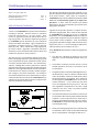
The main objective of incorporating API-650 nozzle flexibilities into a piping analysis is to ensure that the proper loads
can be computed at this point, and that these loads will not
exceed the maximum allowed loads - also determined by
API-650. Although there are three global forces and three
global moments which can be applied to the tank opening, the
radial force, the longitudinal moment, and the circumferential moment are the only three normally considered significant enough to cause shell deformation. The stiffnesses
associated with these three forces and moments are computed and automatically inserted into the CAESAR II analysis
when the user specifies an API-650 nozzle. The figure below
shows the orientation of these loads.
Figure 1
6
The API-650 Appendix P also provides equations to compute the radial growth and longitudinal rotation of the shell
at the nozzle location. These values are computed by
CAESAR II and provided as additional information. These
values are not automatically applied as pre-defined displacements. If these values are desired as pre-defined
displacements, the user must manually specify them on the
piping input spreadsheet.
Appendix P also provides equations to compute the maximum allowed piping loads. These values are also computed
by CAESAR II and provided to the user as additional
information. Once the CAESAR II run has been made, the
restraint loads computed at the nozzle should be compared
to these limits to assure compliance. (Note, the maximum
piping loads computed according to API-650 assume only a
single load is active, i.e. when evaluating the radial force,
API-650 assumes the two moments are zero.)
The CAESAR II implementation of API-650 Appendix P is
as follows:
1.
The data base containing the digitized curves from
Appendix P is located and made available to the program.
2.
The stiffness coefficients, based on the user’s nozzle
and tank parameters, necessary to access these curves
are determined.
3.
Using these stiffness coefficients and the digitized curves,
the dimensionless values are obtained. Based on these
values, the modulus of elasticity and the nozzle radius,
the desired stiffnesses are obtained. These stiffnesses
are then applied by CAESAR II to the nozzle node as
restraint stiffnesses. (Users should note that these
curves from Appendix P are log-log curves. Not only
must logarithmic interpolation be used, but a slight
variation in the curve values can produce stiffness
variations in excess of 50%.)
4.
The unrestrained deflection and rotation of the nozzle
are determined, based on the product head and thermal
expansion. As previously noted, these values may be
used as pre-defined displacements if the user so desires.
CAESAR II will not automatically apply these values
as nodal displacements.
5.
Finally, the limiting piping loads (forces and moments)
are determined. These values are also obtained through
the use of interpolation of the digitized API curves.
COADE Mechanical Engineering News
The input screen necessary to describe an API-650 nozzle is
shown in Figure 2 below. This data is very similar to that
required for a WRC-297 nozzle.
December, 1993
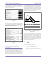
of nozzles, CodeCalc asks the user for the angle between the
nozzle centerline and a tangent to the vessel mean radius, as
also shown in Figures 4 and 5. However, for hillside nozzles,
the determination of this angle can be difficult. The purpose
of this article is to provide a few simple equations that can
help the user determine this nozzle angle.
Figure 2
The results of the API-650 computations are shown in Figure
3. Note that the only quantities used by CAESAR II in the
flexibility analysis are the three stiffness values. All other
data is presented for information only.
Figure 4 - Y-angle Nozzle: Angled in longitudinal
plane of cylinder
The overall goal of this calculation is simple: find an angle
for which the calculated diameter of the hole will match the
actual diameter of the hole. The finished diameter is the
dimension d in Figures 4 and 5, which is called DLR in the
CodeCalc print-outs. If we had the nozzle in front of us and
could measure d, then we could calculate the input angle very
simply using the following equation:
sin α
α
α=
Figure 3
dn
d
where: dn = inside diameter of nozzle
CodeCalc: Hillside and Off-Angle
Nozzle Angles
d = DLR = finished diameter of hole
sin α
α
α= sine of angle between nozzle and vessel
There are two main categories of off-angle vessel nozzles:
those which are off-angle in the longitudinal plane of the
cylinder (Y-angle nozzles, Figure 4), and those which are off
angle in the circumferential plane of a cylinder, or in a head
(Hillside nozzles, Figure 5). In order to analyze these kinds
7
COADE Mechanical Engineering News
December, 1993
FL − r I
Hr K
L+r I
α
α
α = arccos F
Hr K
n
α
α
α1 = arccos
m
n
2
m
α
α
α=
α
α
α1 + α
α
α2
2
where: L = offset distance cylinder/head centerline
rn = inside nozzle radius
rm = mean vessel radius
Figure 5 - Hillside Nozzle
When we analyze Y-angle nozzles, the angle is known and
the result is exact — this is really all the information we need.
d = DLR =
dn
α
α
sin α
However, when we analyze hillside nozzles, as shown in
Figure 5, the angle is usually not known. Instead, we may
know the offset distance for the nozzle. This distance, L, is
the distance between the centerline of the cylinder or head,
and the centerline of the nozzle. A first approximation to the
angle would take the cosine of the angle as L / rm, where rm
is the mean cylinder or head radius at the point of attachment.
However, this approximation turns out to be too inaccurate
for normal use.
The ASME Code has a sample problem, L-7.7, which shows
what their preferred method is. (They do not explicitly
address this off-angle problem in the body of the Code.)
Figure 6, taken from ASME, Section VIII, Division 1,
Addenda A92, page 512, shows this sample problem. The
key to their approach is the calculation of two angles, α1 and
α2, and then the calculation of the finished diameter from the
difference between these two angles. You can follow their
calculation on page 512 and 513 of the Code. For our
purposes, we do not need to carry the calculation that far.
The angle we are looking for is just the average of the two
Code angles, calculated as:
8
Figure 6 - ASME Code Figure L-7.7
These three equations can be used without any further
information for any hillside nozzle in a cylinder. However,
you need to apply them carefully to hillside nozzles in heads.
When a hillside nozzle is in an elliptical or torispherical
head, the nozzle may be located in the spherical portion of
the head, the toroidal portion of the head, or it may straddle
the two portions. This is shown in Figure 7. Each of these
cases requires a slightly different L and rm to be used in the
equations.
When the nozzle lies entirely within the spherical portion of
the head (Figure 7(a)), L is simply the offset from the head
centerline, and rm is the spherical radius of the head. For
spherical or torispherical heads this should be a known
COADE Mechanical Engineering News
radius (Code dimension L in Figure 1-4 of Appendix 1). For
elliptical heads, the spherical portion is taken to be a circle
drawn on the head with a diameter of 80 percent of the head
diameter. The radius of the spherical portion is taken to be
0.90 times the head diameter. The nozzle offset from the
vessel centerline should be known from the vessel drawings.
The nozzle can also lie entirely in the knuckle portion of the
head (Figure 7(c)). The mean radius (rm) is the mean knuckle
radius, and the offset (L) is the distance from the origin of the
knuckle radius to the centerline of the nozzle. Note that for
an elliptical head, the knuckle is defined as anything outside
a circle drawn on the head with a diameter of 80 percent of the
head diameter. The knuckle radius is 0.17 times the vessel
diameter.
December, 1993
Finally, the nozzle may be located so that part of the nozzle
is in the spherical portion, and part in the knuckle (Figure
7(b)). In this case, the angle at the part of the nozzle in the
spherical portion should be calculated as described for
Figure 7(a), and the angle at the part in the knuckle portion
should be calculated as described for Figure 7(c). That is,
calculate the inside angle using the spherical radius of the
head and offset from the centerline. Calculate the outside
angle using the mean radius of the knuckle and the offset
from the knuckle origin.
Use of these equations should yield correct nozzle angles for
almost all off-angle nozzle configurations.
An Introduction to Time History Analysis
With the release of CAESAR II Version 3.20, users can now
perform linear modal time history analysis of dynamic events
imposed on piping systems. (This analysis technique provides
a true simulation of the dynamic system response as a
function of time due to the imposed load, and is usually more
accurate than the corresponding response spectrum method.)
This article will introduce this analysis technique through the
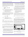
use of a cantilever beam model, as well as demonstrate its
accuracy in simulating dynamic response. This cantilever
beam is described in Figure 8 below.
Figure 8
Figure 7 - Hillside nozzles in heads
This cantilever beam is a 4 inch standard wall, low carbon
steel pipe. The diameter, wall thickness, density, elastic
modulus, and fluid density are shown in the figure. Notice
that the length is 116.544 inches and a point load of 403.3
pounds is applied at the free end. These two values are
9
COADE Mechanical Engineering News
somewhat contrived so that the results and behavior of the
beam are predictable. The length was obtained such that the
first natural frequency of the beam is exactly 10 Hz, which
corresponds to a period of 0.1 seconds. The first natural
frequency of a cantilever beam modeled as a series of lumped
masses can be calculated as:
f=
F1 πππIe3EIg / ∑ dW ∗ X ij
H2 K
where: g =
Wi =
E =
I =
Xi =
i
3
i
1
2
acceleration of gravity = 386.088 in/sec2
weight of the pipe and fluid lumped at node (i)
Young’s modulus of pipe material
moment of inertial of pipe
distance of node (i) from fixed end
Alternatively, one could turn to a reference, such as Marks'
Standard Handbook for Mechanical Engineers, 9th Edition.
Page 5-74 provides the following equation for the first five
natural frequencies of a cantilever beam:
where: w = weight per unit length of the beam
L = length of the beam
cn = coefficients defined in the Table below
Frequency:
cn value :
1
0.56
2
3.57
•
The same load applied to a critically-damped system
should produce a response which goes through one
cycle before stabilizing at the static displacement.
•
The same load applied to an over-damped system should
produce a response which does not cycle at all. Rather
the displacement slowly attains the static magnitude.
Entering the CAESAR II dynamic input module and selecting “Time History” as the analysis type reveals that data in
the following input forms must be specified (all other input
forms are optional for this type of analysis).
3 Spectrum/Time History Definitions
7 Spectrum/Time History Force Sets
9 Spectrum/Time History Load Cases
B Control Parameters
(For the purposes of this example, since only motion in the
vertical plane is of interest, the “1 - Lumped Mass” option
was used to zero the masses in the X and Z directions.)
For the “3 - Time History Definition”, the impulse is defined
as:
1
2
e c hj
fn = c n ∗ gEI / wL4
December, 1993
3
9.82
4
19.2
5
31.8
Once the length of the beam is known, the load required to
produce a static deflection of 1 inch was determined from:
CANT TIME FORCE LINEAR LINEAR
which states that the impulse name is “CANT”, it is a time
verse force curve, and linear interpolation should be used for
both axes. Only two data points are necessary to describe
this impulse; point 1 is at 0.0, 1.0, and point 2 is at 3000.0,
1.0. This defines a straight line (instantaneous) impulse
from 0.0 to 3000 milliseconds with a multiplier of 1.0.
(Alternatively, the force of 403.3 pounds could been entered
here.) This impulse is shown in Figure 9:
P = (1.0) * 3 * E * I / L3
where “P” is the tip load, and all other terms are defined
above. The value of “P” is computed as 403.3 pounds.
The objective of the analysis is to determine if the dynamic
response of the beam under the time history matches the
expected results (i.e. as predicted by dynamic theory). For
example:
•
•
10
A load applied instantaneously to an un-damped system
should yield twice the displacement of the same load
applied statically. Additionally the system should cycle
between plus and minus this displacement forever.
The same load applied to an under-damped system
should show close to the same initial displacement, but
further cycling decays the displacement magnitude.
Figure 9
For the “7 - Time History Force Set”, the magnitude and
direction of the impulse are specified as:
-403.3 Y 1100 1
which states that a load of -403.3 pounds is applied in the Y
COADE Mechanical Engineering News
December, 1993
direction at node 1100 and is associated with force set
number 1.
For the “9 - Time History Load Cases”, the force set is
associated with the impulse as follows:
CANT 1 Y 1
which states that the impulse curve CANT is included in the
load case with a scale factor of 1.0, in the Y direction, and it
acts on the load from force set 1. The total load applied to the
system is the product of the force multiplier times the force
set load times the load case scale factor.
For the “B - Control Parameters” screen, the following items
must be specified:
TIME <—-Analysis Type (HARMONIC/SPECTRUM/MODES/RANGE/TIMEHIST)
5
1.0
.2
0.03
40
<—<—<—<—<—-
Max. No. of Eigenvalues calculated (0-Not used)
Closely Spaced Mode Criteria/Time History Time Step (ms)
Load Duration (Time History or DSRSS method) (sec.)
Damping (Time History or DSRSS) (ratio of critical)
ZPA (Reg. Guide 1.60 — g’s)/# Time History Output Cases
The analysis type should be set to “TIME”. The analysis is
configured to extract and use the first five natural frequencies. The value for the time step is set such that the time step
multiplied by the maximum frequency is less than 0.1, which
yields a value of approximately .001 seconds. (Actually the
lowest frequency was used here, since it dominates the
system displacement response by a wide margin, as can be
seen by a review of the Participation Factor report.) The
duration is recommended to be at least as long as one full
cycle, based on the lowest frequency (highest period). The
fundamental period of this beam model is 0.1 seconds, so a
duration of 0.2 seconds should produce two full cycles. The
number of requested reporting cases was set at 40, providing
reports (displacements, forces, stresses) every 5 milliseconds.
The value for the damping ratio was varied to show not only
the effects of damping, but to provide data to visualize the
response of the beam. (The damping ratio is the ratio of the
actual damping to the critical damping. Values less than 1.0
are indicative of under-damped systems, while values over
1.0 are indicative of over-damped systems, and a value of
exactly 1.0 indicates a critically damped system.) Five runs
were made with the damping ratio set to 0.0, 0.03, 0.5, 1.0,
and 2.0. For each run, the “Y” displacement at the tip of the
cantilever (node 1100) as a function of time was stored in a
data file. A plot of this data (generated using the 2-D plotting
module of CAESAR II) is shown in Figure 10.
Figure 10
The curve for a damping ratio of zero (DR=0.0) represents
the response of an un-damped system. The curve shows that
the maximum response peaks at just less than -2 inches,
which is the expected result. Additionally, the curve shows
that a full cycle of response is attained every 100 milliseconds, as expected. This curve also shows that the vibration
of an un-damped system does not diminish with time, i.e. the
amplitude of the response for each cycle remains constant.
Also notice that the motion is cycling about the magnitude of
the static displacement of -1.0 inches. All of these
characteristics of the “DR=0.0” curve are as expected.
The curve (with the diamond symbols) for a damping ratio of
0.03 (DR=.03) represents the response of a typical piping
system. The maximum and minimum response values occur
at multiples of the first natural period, as in the un-damped
case. However, as can be seen in the figure, the amplitude of
the response continuously decays with time. This behavior
can be shown further by extending the analysis for a duration
of 2 seconds. The resulting plot of the tip displacement in the
11
COADE Mechanical Engineering News
December, 1993
“Y” direction is shown in Figure 11.
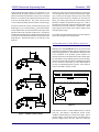
universal, tied expansion joint. Reviewing the input matrix
for the CAESAR II expansion joint modeler, one finds there
are at least six assemblies available (see Fig. 12). Each
assembly must have its advantages, so what are they? This
article will examine these and other assemblies to highlight
their individual uses.
Figure 12
Figure 11
In Figure 10, the curve (with the clover symbols) for a
damping ratio of 0.5 (DR=0.5) represents a highly damped,
though still under-damped system. The oscillations after the
first cycle are barely noticeable, and in fact die out after 1.5
cycles. The curve (with the spade symbols) for a damping
ratio of 1.0 (DR=1.0) represents a critically damped system.
The response for this run shows that the static displacement
is attained in one cycle, after which there are no further
oscillations. The curve (with the heart symbols) for a
damping ratio of 2.0 (DR=2.0) represents an over-damped
system. As the figure shows, the response for an overdamped system is not much more than a slow static response.
These results and a study of Figure 10 show that the behavior
of a cantilever beam in a CAESAR II time history analysis
is as predicted by theory. This article also illustrates the ease
with which a time history analysis can be implemented using
CAESAR II.
Selecting and Evaluating
an Expansion Joint Assembly
Pipe is quite rugged. High loads and stresses in the piping do
not justify the installation of an expansion joint. The
equipment to which the piping is attached is another story. In
many cases the piping attached to rotating equipment may be
loaded to only 5% of its allowable so that the pump, compressor, or turbine loads do not exceed their allowable limits.
This low load limit must be handled in both the cold and hot
piping positions. Adding or adjusting supports should
reduce the cold loads on the equipment, but the change
between the hot and cold loads is a function of the thermal
loads and the piping flexibility — adding flexibility is the
purpose of the expansion joint. How much room is available
for the joint and what sort of load must be decreased
determines what expansion joint configuration should be
used. Clearly identifying the force or moment to be reduced
is the first step in specifying an expansion joint assembly.
What type of joint arrangement should be used? To quickly
review the different expansion joint assemblies, just page
through any expansion joint manufacturer’s catalog. On a
more generic level, one would refer to A Practical Guide to
Expansion Joints by the Expansion Joint Manufacturers
Association, Inc. (25 North Broadway, Tarrytown, NY
10591). This booklet describes the parts of an expansion
joint, how to design a system containing expansion joints,
and recommendations on proper installation and handling.
Closer to home, the CAESAR II expansion joint modeler
offers the following:
•
The basics of the CAESAR II Expansion Joint Modeler
appeared in the last issue of Mechanical Engineering News
(The CAESAR II Expansion Joint Modeler - Volume 16).
This article reviewed important model characteristics of the
joint and discussed how the program modeled a simple
expansion joint. The article did not indicate how a particular
assembly was selected. For example, why would one
recommend a simple, untied expansion joint instead of
12
UNTIED (Single Expansion Joint) — The simplest
assembly, a single joint has no restrictions on its motion;
but, except for hoop stress, it also has no pressure
containing capabilities. In exchange for providing the
most freedom, this joint requires special care in overall
design. The piping around the joint must be well guided
to prevent any squirm in the joint that would be further
aggravated by pressure thrust on the joint. Simple
expansion joints also require axial stops or anchors
COADE Mechanical Engineering News
somewhere up and down the line to absorb the pressure
thrust load. So with all the freedom in this joint, the
pressure containment requirements reduce its flexibility (in most applications) to only the axial direction. A
Double Expansion Joint is a related configuration. This
is an assembly of two single joints separated by a short
run of pipe. The pipe separating the two joints is usually
restrained from motion by an anchor. The use of a
double joint is the same as a single joint but it can share
the total axial deflection between the two joints.
•
•
TIED (Single Tied Expansion Joint) — Pressure thrust
on the joint may be contained without adding anchors
and guides to the attached piping. Instead, the axial
thrust is checked by the addition of tie rods around the
joint. These tie rods drastically alter the nature of the
joint. When untied, the joint provides flexibility in the
axial direction. Now tied, the joint is essentially rigid in
the axial direction, but lateral flexibility is available to
the designer and no additional thrust blocks or guides are
required. A simple, tied expansion joint, then, is installed
perpendicular to the plane of required
flexibility.
HINGED (Hinged Expansion Joint) — Tie bars on
either side of a single expansion joint may also be
hinged. With a single joint, though, the only allowed
motion is angulation, not axial or transverse deflection,
and angulation about the one hinge axis only. Hinged
joints are quite compact and they easily contain the
pressure thrust loads. In many cases, two or even three
hinged joints work together to provide needed flexibility. Hinged joints often require guides to drive the
piping into the flexible direction.
•
GIMBAL (Gimbal Expansion Joint) — Gimballed joints
combine two, perpendicular, hinges across an expansion
joint. These bars, from either end of the joint, hinge off
a ring at the center of the joint. This articulated joint
allows bending about both axes perpendicular to the axis
of the joint. Gimbal joints are usually used with other
gimbal joints or hinged joints and with pipe guides.
Guides are used to force motion in a line perpendicular
to the hinge axes of the joints.
•
U-UNIV (Universal Expansion Joint) — A universal
expansion joint is a double joint without an anchor on the
center spool piece. The lack of restraint on the center
piece turns it into a linkage between the two joints. This
linkage assembly converts the joints’ bending flexibility
into large transverse displacements. A longer center
piece produces greater transverse offsets with the same
bending on each joint. However, the lack of restraints or
other pressure containing elements limits the application
of this joint to low pressure lines.
December, 1993
•
T-UNIV (Universal Tied Expansion Joint) — As the
name suggests, these are assemblies that have a universal expansion joint configuration with a set of tie rods
running over both joints to contain the pressure thrust in
the line. The tie rods would also have some means of
attachment to the center spool piece to stabilize the
entire unit. Here again, the tie rods eliminate any axial
flexibility but permit a great range of transverse movement through the bending of the two joints. The greater
the length of the center pipe, the greater the transverse
deflection with the same amount of joint bending.
Other configurations of note:
•
Swing Expansion Joint — Some piping configurations
require transverse flexibility in one direction but not the
other. In these situations, a swing expansion joint is
recommended. A swing joint is similar to a tied universal joint in that it has a pair of bellows and a center spool
piece. Instead of tie rods, the swing joint will have
hinged bars restraining the pressure thrust. The parallel
hinges at either end of the assembly allow bending about
only one axis rather than two. These joints therefore
direct the transverse deflection of the joint along a
defined vector perpendicular to the axis of the expansion joint assembly.
•
Pressure-balanced Expansion Joint — Utilization of
axial flexibility in an expansion joint usually requires
the joint to be untied and heavily guided. Tie rods, while
containing the pressure thrust forces, eliminate axial
flexibility of an expansion joint. Another way of keeping
axial flexibility without adding extra guides and thrustresisting anchors is by using pressure-balanced expansion
joints. A way of understanding this axial flexibility is to
examine the center spool piece of a universal tied
expansion joint. This center piece is relatively free to
move axially. It is not affected by the pressure thrust as
that load is carried across the entire joint through the tie
rods. The center spool piece is resisted only by the axial
stiffness of the attached expansion joints. If the piping
ran out through the center spool piece (by placing a tee
in the spool piece) and the pipe after the tie rods is
capped, then the axial (or lateral) flexibility remains.
Additional hardware is needed for the proper installation on
several types of expansion joint assemblies. Guides are
required to drive the piping in a specific direction so that the
joint deflects in a controlled and safe manner. Pressurized
joints without tie rods or hinges require anchors to hold the
pressure thrust load. In most instances, this pressure thrust
load is contained by the pipe wall. The flexibility of the joint
cannot limit the axial deflection of the pipe due to pressure
and so this thrust must be held elsewhere upstream and
13
COADE Mechanical Engineering News
downstream from the untied joint. Any supports on the line
must be examined to confirm their ability to withstand the
pressure thrust load. CAESAR II (as most any other pipe
stress analysis program) does not automatically incorporate structural analysis of pressure loading. It is up to the
analyst to confirm that the load is of correct magnitude and
applied at an acceptable location on the pipe. CAESAR II
will apply the pressure thrust load on either end of an untied
joint but this is only a good approximation. The properly
located thrust load may be determined by imagining a position
inside the joint; the pipe wall seen upstream and downstream
from the joint is the proper point to apply the pressure thrust
load. This point may be beyond a support that was assumed
to contain the pressure thrust.
Expansion joint assemblies add flexibility to a piping system; that is certainly understood. What may not be so clear
is that these assemblies cannot supply flexibility in all
directions. The requirement to restrain the pressure thrust
load must still be satisfied and this requirement will eliminate
one or more flexible degrees or freedom from the configuration. One way, then, of categorizing the various assemblies
is to examine the available flexibilities of these joints:
Type
Freedom
Notes
UNTIED
axial
lateral & bending with low
pressures, reqs. guides and
thrust supports
TIED
lateral
compact and stable
HINGED
bending
(one axis) used in combinations for lateral flexibility,
guides recommended
GIMBAL
bending
(both axes) see above
U-UNIV
lateral
stable only for low pressure
applications, total offset determined by length of center
piece
T-UNIV
lateral
total allowable offset is a function of center piece length
Press. Bal.
“axial”
used with a bend or tee on
center piece so it may be considered lateral, provides axial
flexibility without additional
pipe supports
Expansion joint assemblies, then, can be selected based on
their ability to provide flexibility in specific directions, their
14
December, 1993
space requirements, and their support requirements. This
article presents a sensible way to address the variety of
configurations available to the piping system designer. The
next issue of Mechanical Engineering News will review
individual joint selection and evaluation.
Estimation of Nozzle Loads Using
CAESAR II Software
Results of pipe stress analysis (or, for that matter, any
structural analysis) can vary depending upon the assumptions made when modeling the problem. For example, the
best means of defining boundary conditions, loading combinations, and material/element behavior is rarely clearly
defined. For this reason, modeling conventions often develop in order to simplify the decision making procedure — or,
so the engineer need not reinvent the wheel for every new
problem.
In the pipe stress field, each piping code normally has
modeling conventions associated with it, which have been
found to produce the best estimate of pipe stresses under
loadings normally associated with the industry to which the
particular code applies. For example, the B31.1 Power
Piping Code, used in an industry where pressures may not get
high enough to significantly stiffen pipe, does not consider
pressure stiffening during the calculation of flexibility factors
of elbows. Likewise, pressure strain effects are usually
included only on very long runs of highly pressurized pipes,
such as might be found on cross-country gas transmission
pipes, covered by the B31.8 Gas Transmission Piping Code.
Also, the different piping codes have their individual
conventions for calculating the stress intensification factors
of local components.
The true behavior of the piping system under load is much
more complex than that of any linear system solved by a pipe
stress program. Evidence that the best assumptions for
modeling piping systems are not hard and fast is indicated by
the diversity of the various code requirements. One thing
that is certain, however, is that the means of calculating pipe
stresses for each code (which vary for every code) has been
proven to be adequate when compared to the means of
calculating the allowable stresses for the same code (which
also vary from code to code).
However, the conventions chosen as best for stress calculation purposes may not provide the best means of maximizing
the accuracy of other results — displacements, reactions,
etc. — which are not addressed in as much detail by the
codes. Nozzle loadings also vary by code (or more accurately, vary by modeling conventions, which may vary by code),
COADE Mechanical Engineering News
whereas the allowables do not, since they are set by the
equipment manufacturers or according to standards of third
parties, such as the American Petroleum Institute. Therefore
it is important to get as accurate an estimate as possible of
nozzle loads, independent of the particular code’s modeling
conventions. A single analysis, conducted for code compliance purposes, may show that the nozzle loads are well within
the equipment’s nozzle allowables. However, altering the
modeling conventions may cause the loadings to vary
significantly — in fact, far more than do the maximum system
stresses. In some cases, it may be advisable to do several
analyses, with different modeling assumptions, in order to
determine the potential range of results.
Consider the system of which a portion is shown in Figure 13.
This system represents a 42"-diameter, 1-1/2" wall, gas
transmission pipe, with an internal pressure of 1000 psig.
The pipeline originates at an anchor (not shown), and runs
approximately one mile, with two expansion loops in the
vertical plane, before turning horizontally as it enters a
compressor station. The system temperature is expected to
vary from an ambient of 70oF to a maximum of 100oF. The
line is connected (restrained in six degrees-of-freedom) to a
compressor nozzle at node point 360.
December, 1993
case), of 1185 lb (FX), -7745 lb (FY), 15025 lb (FZ), -30279
ft-lb (MX), 220575 ft-lb (MY), and 2697 ft-lb (MZ), which
should be checked against the manufacturer’s allowables,
may be acceptable as well.
As noted above, the stress calculation is perfectly acceptable
here, since the B31.8 allowable stresses take into consideration the modeling conventions normally associated with
this code. The nozzle load calculations may be a different
matter; the analyst should be more interested in finding a less
code-dependent result. This can be done by re-analyzing the
system with a few different modeling conventions — the true
nozzle loads probably fall somewhere within the range of the
results. The results for a number of modeling conditions are
shown in Table 1. The analyses shown in this table were
generated by making the following changes to the original
model:
NOZZL1 — This model is identical to the original, except
that pressure stiffening of the elbows is neglected. This
matches the treatment of elbow flexibilities as endorsed by
the B31.1 and other piping codes. Pressure stiffening reduces the flexibility of elbows by dividing the flexibility factor
by:
[1 + 6 (P/E) (r2/T)7/3 (R1/r2)1/3]
Where:
P = internal pressure, psi
E = modulus of elasticity of pipe material, psi
r2 = mean radius of pipe, in
T = wall thickness of pipe, in
R1 = bend radius of elbow, in
For this application, the flexibility factor is reduced by a
factor of 1.128.
Figure 13
The initial analysis, done under the B31.8 Code using
CAESAR II’s defaults (i.e., pressure stiffening of elbows,
absence of pressure strain effects, default rigid stiffnesses for
all restraints and the anchor to the compressor, etc.) yielded
the results shown for the first case (labeled NOZZLE) in
Table 1. The maximum system Operating, Sustained, and
Expansion stresses of 9538 psi, 7679 psi, and 3090 psi,
respectively (with the maxima occurring at various points
along the run), are acceptable against the code allowables.
The nozzle loads on the compressor (for the Operating load
Pressure stiffening of elbows can be activated, de-activated,
or used as per the specific requirements of the code in use by
setting a parameter in the CAESAR II configuration file
(Option 9 of the Main Menu).
NOZZL2 — This model is identical to the original, except
that pressure stiffening of straight pipes is included. This is
the phenomenon that occurs when the sag of a guy-wire is
reduced as it is tightened — likewise, a beam highly stressed
in tension will deflect less under a lateral load than would the
same beam subject to compressive stresses. The effect of
tensile stresses on bending of a beam can be determined by
15
COADE Mechanical Engineering News
examining the element shown in Figure 14:
December, 1993
respect to x:
εx = u' - y θ' + θ'2 / 2
Where:
u' = first derivative of axial strain (with respect to x)
y = distance of point of interest from neutral axis
θ' = first derivative of angle of curvature (with
respect to x)
Figure 14
Total elemental strain energy U (considered over the entire
length and the entire cross-section) is calculated as:
Initially assuming the beam in the figure is infinitely stiff in
bending (so it is straight in any configuration), but can
deform axially, the total axial strain (for small lateral displacements) is constant over the cross-section, and is computed as:
εx = εu + εv
zz
U=
zz
L
0
A
1
E εεεx2 dA dx
2
L
0
A
1
E u' − y θθθθ' 2 / 2
2
2
dA dx
Where:
E = material modulus of elasticity
Where:
εu = axial strain due to axial load
= (u2 - u1) / L
U=
A = cross-sectional area of element
Noting that (for a prismatic member):
u2 = axial displacement at node 2
zdA = A
zy dA = 0
zy2 dA = I
zEu' dA = P
u1 = axial displacement at node 1
L = length of beam
εv = axial strain due to rotation of the bar through a
small angle θ while holding x-motion constant
= (1/cos θ) - 1 = (sec θ - 1) = θ2/2
≈ [(v2 - v1)/L]2/2
Where:
v2 = lateral displacement at node 2
I = moment of inertia of element
v1 = lateral displacement at node 1
P = axial force acting on element cross-section
If the beam is capable of bending, then the axial strain is no
longer constant over the cross-section, since bending puts the
cross-section in varying levels of compression and tension,
based upon the distance to the neutral axis. For this case, the
axial strain is a function of the distance from the neutral axis.
An additional term must be added representing the rotation
of the element face, and the εv term must be modified to take
into consideration the fact that it is no longer linear with
16
The elemental strain energy can be written as:
U=
zAE / 2 u'
L
0
2
dx +
zaEI / 2 fθθθθ' dx + zaP / 2 fθθθθ' dx
L
0
2
L
0
2
The first integral in the expression above provides the
standard stiffness matrix for a truss element (or the axial
terms of the stiffness matrix for a beam element). The second
COADE Mechanical Engineering News
December, 1993
integral provides the lateral and rotational stiffness matrix for
a beam element. These are the only stiffness terms that are
included in CAESAR II’s default stiffness matrix formulation (as well as that of virtually all other stiffness method
programs).
The third integral however, represents the work done when
differential elements (of size dx) are stretched an amount of
θ'2dx/2 by an axial force P. From this integral, then, the stress
stiffening matrix [Ks], which should be added to the default
element stiffness matrix, can be derived. Equating strain
energies:
z
z
1
L
kp K kp
d = a
P / 2f
θθθθ' dx = kp
d M
2
N
1
d
2
L
T
s
2
0
T
L
G
T
P G dx
0
O
d
P
Qkp
Since:
θ = [N]{d}, and
θ' = [G]{d}
Where:
Ks
0
L
M
0
M
P M0
=
M
30 L M0
M
0
M
M
N0
36
3 L 4 L2
0
−
0 0
36 − 3 L 0
3 L − L2 0 −
O
P
P
P
P
P
P
36
P
3L 4 L P
Q
2
Note that the upper triangular portion of the matrix is
symmetric about the main diagonal.
Activating pressure stiffening of straight pipes in CAESAR II
simply applies the stress stiffening matrix to the elemental
stiffness matrices (of straight pipes only), using an axial
force P equal to the internal pressure (user selectable P1 or
P2) times the internal area of the pipe. Note that other
internal forces (due to thermal or imposed mechanical loads)
are not included in the P force — this is not a non-linear
effect. This option is activated by entering 1 (to use pressure
value P1) or 2 (for pressure value P2) on the Use Stress
Stiffening due to Pressure entry under Special Execution
Parameters of the Kaux menu.
{d} = vector of elemental displacements
[G] = first derivative (with respect to x) of elemental
shape function matrix [N], with on diagonal
entries of:
G1 =
G2 =
G3 =
G4 =
G5 =
G6 =
0
-6x/L2 + 6x2/L3
1 - 4x/L + 3x2/L2
0
6x/L2 - 6x2/L3
-2x/L + 3x2/L2
NOZZL3 — This model is identical to the original, except
that pressure strain effects (often called the Bourdon effect)
have been included. This effect considers the elongation of
pipes under pressure tensile stresses as a loading condition.
For example, the piping codes generally require that pressure
be considered as having not a strain component, but only a
stress component, which should be simply added to the
calculated sustained stresses:
Ssus = PDi2/(Do2-Di2) + iM/Z
Where:
[N] = elemental shape matrix, with on diagonal
entries of:
N1 =
N2 =
N3 =
N4 =
N5 =
N6 =
0
1 - 3x2/L2 + 2x3/L3
x - 2x2/L + x3/L2
0
3x2/L2 - 2x3/L3
-x2/L + x3/L2
Ssus = total sustained stresses
P
Di = internal diameter of pipe
Do = external diameter of pipe
i
Carrying through the matrix multiplication and the integration, the additional stiffness due to axial force is found to be:
= internal pressure
= stress intensification factor
M = moment on cross-section due to non-pressure
sustained loads
Z
= section modulus of pipe
17
COADE Mechanical Engineering News
For straight pipes, the pressure strain can be calculated in a
straight-forward manner. Longitudinal pressure stresses
cause longitudinal strains (approximately equal to Pri/2tE),
which are reduced by the Poisson contraction due to the hoop
and radial stress (approximately equal to -2υPri/2tE), for a
net longitudinal strain of:
ε = (1 - 2υ) Pri/2tE
Where:
ε = longitudinal pipe strain due to pressure
υ = poisson’s ratio
P = internal pressure
ri = internal radius of pipe
t = pipe wall thickness
December, 1993
original Mare Island piping flexibility program written in
1959) and Crocker & King’s Piping Handbook, 5th Edition
(pages 4-37 through 4-38) alternatively view pipe bends as
behaving similarly to Bourdon tubes — hence the popular
name Bourdon effect for pressure elongation (note that
pressure strain of straight pipes is calculated the same under
both methods).
Bourdon tubes are flattened tubes of steel bent into a circle,
which tend to straighten out when pressurized. This introduces a angular change in the tube (or, accordingly, the pipe
bend) as the tube opens up under pressure. (It is COADE’s
contention that the Bourdon tube straightens as a consequence of the flattened tube trying to develop a round crosssection, so this effect should not really apply to a forged pipe
elbow, which already has a truly round cross-section. It may
have some validity when discussing bends which have been
bent from straight pipe.)
MEC-21’s derivation of the end rotation and displacement
strains of a pipe elbow under pressure are shown below:
E = modulus of elasticity of pipe material
For elbows, the calculation of the end displacements is more
complex. Assuming that the pressure strain is constant
throughout the length of the bend, the bend end distortion can
be modeled similarly to that for uniform thermal growth.
From Roark and Young’s Formulas for Stress and Strain (5th
Edition), the end displacement and rotation of a curved beam
under uniform strain is given by:
d = 2εRsin(θ/2) = (1 - 2υ) Pri Rsin(θ/2)/tE
c
φφφφφ= π
πθ
πθ
πθθP ri 4
ha2 − 2 υυυfa
+ 3 − 1. 5 υυυf
r / R /a
2 EI f
bsin θθθθ− θθθθg
a=b
φφφφφR / θθθθg
2
b
gb
Where:
a = displacement in direction a (as per Figure 15)
c = displacement in direction c (as per Figure 15)
φ=0
d = displacement of bend (directionally along line
through ends)
R = bend radius
θ = included angle of bend, radians
φ = change in angle of bend
These pressure strains can be incorporated into the analysis
(and were, for analysis NOZZL3) by entering 1 on the
Activate Bourdon Pressure Effects entry under Special
Execution Parameters of the Kaux menu.
18
g
c = φφφφφR / θθθθ cos θθθθ− 1
Where:
NOZZL4 — This model is similar to case NOZZL3 described above, except that the pressure strain effects have
been applied in a slightly different way — using the “true”
Bourdon effect. A number of sources, such as MEC-21 (the
2
i
Figure 15
COADE Mechanical Engineering News
December, 1993
The full Bourdon effect, considering the rotational effect of
the elbows as per MEC-21 was incorporated into this case by
entering 2 on the Activate Bourdon Pressure Effects entry
under Special Execution Parameters of the Kaux menu.
NOZZL5 — This model contained more than one of the
effects described above — pressure stiffening of elbows,
pressure stiffening of straight pipes, and Bourdon effect
number 2. This would probably be a better model of reality
in that these effects would not occur in isolation.
NOZZL6 — This model was identical to the original case,
except that stiffnesses of 1E6 lb/in and 1E6 in-lb/deg were
used for the translational and rotational stiffness respectively
at the compressor connection. This is not necessarily a
representative value; however, it is certain that the compressor connection is not infinitely rigid, and this case can be used
to give an indication of how much the results may be affected
by modeling the compressor stiffness. The true measure of
compressor rigidity may be estimated through finite element
analysis, test, manufacturer’s documentation, or other means.
RESULTS AND CONCLUSION: The maximum and
minimum values were tabulated for the six components of the
compressor nozzle load, as well as the maximum Operating,
Sustained, and Expansion stress of any point in the system for
the seven versions of the model. These results are shown in
Table 1.
Compressor Nozzle Loads (OPE Case)
Case
FX
FY
FZ
MY
MZ
OPE
(ft-lb)
SUS
EXP
1185
-7745 15025 -30279 220575 2697
9538 7679 3090
NOZZL1
1107
-7777 13876 -30519 201406 2683
9750 7900 3251
NOZZL2
1415
-7923 16725 -29702 194005 2483
9376 7662 2964
NOZZL3
1734
-7751 21974 -30320 322520 2687 11029 8050 3090
NOZZL4
2028
-7753 25834 -30340 380473 2683 11873 8878 3090
NOZZL5
2398
-7927 28396 -29734 335800 2475 11605 8746 2964
MAX MAG
2398
-7927 28396 -30519 380473 2697 11873 8878 3251
MIN MAG
1107
-7745 13876 -29702 194005 2475
NOZZL6
% VAR
117%
1859
32%
2%
105%
-6424 12094
23%
Therefore it is clear that nozzle load calculations, which
should be independent of piping code used (and its associated modeling conventions), may be more sensitive to modeling variations than code stress calculations would be. For
this reason, the engineer may be interested in performing
more than one analysis in order to determine the extremes of
loading which the equipment may be expected to endure.
3%
-45
96%
14394
141% 67820%
Table 1
CAESAR II Specifications
(psi)
NOZZLE
% VAR
In case NOZZL6, where the nozzle flexibilities are introduced, the results are even more striking. Selected components of the maximum tabulated nozzle loads were higher by
141% (FZ), 67,820% (MX), 2711% (MY), and 2724% (MZ)
vs. the results with this model. Meanwhile, the stresses vary
by only 27%, 15%, and 15% for the Operating, Sustained,
and Expansion cases respectively. Even though this may not
be a fully realistic case, this effectively represents the impact
that modeling of flexibilities may have on nozzle loads,
without necessarily providing a corresponding effect on the
stress calculations.
Max System Stress
MX
(lb)
Considering only models NOZZLE through NOZZL5, some
nozzle load components were seen to vary (from the minimum to the maximum) by such large numbers as 117% (FX),
105% (FZ), and 96% (MY). Unexpectedly, the ranges
between the minimum and maximum code stresses were
much smaller, with differences of only 27% (Operating),
16% (Sustained), and 10% (Expansion).
9%
100
2711% 2724%
9378 7662 2964
27%
Class 1
16% 10%
9366 7718 2835
27%
Listed below are those bugs/errors/omissions in the
CAESAR II program that have been identified since the last
newsletter. These items are listed in two classes. Class 1
errors are problems or anomalies that might lead to the
generation of erroneous results. Class 2 errors are general
problems that may result in confusion or an abort condition,
but do not cause erroneous results.
15% 15%
1) Piping Element Generator: A restraint direction cosine
tolerance error has been discovered in Version 3.19.
This error only affects skewed restraints with direction
cosines greater than 0.9998 (angles less than 1.146
degrees).
The original tolerances were set at 0.999 (2.56 degrees),
and at user requests were changed in Version 3.19 to
0.99999 (0.256 degrees). The limits in the Element
Generator (of 0.9998) were overlooked. This error has
been corrected in Version 3.2.
19
COADE Mechanical Engineering News
2) Piping Error Checker: An error has been discovered in
the routine which combines models for the “large job
include”. This error caused some of the allowable stress
data, on the first element of the included job, to be lost.
This error has been corrected in Version 3.2.
This error only affects the first element of the included
job if allowable stresses, different from the preceding
job, were entered.
Class 2
1) Static Output Module: A labeling error was discovered
with regard to the Basic Engineering spring hangers.
Figure BE400 was incorrectly labeled BE404. This
error has been corrected for Version 3.2.
2) Static Output Module: Version 3.19 provided access to
the intermediate data generated by the error checker
(flexibility factors, expansion coefficients, minimum
wall thickness, etc.) when an input echo was requested.
This data was intended to be available when the output
was directed to either the printer or a disk file. Unfortunately access to the printer for this data was omitted
from this version. This oversight has been corrected in
Version 3.2.
3) Batch Stream Processor: The Batch Stream processor
provided in Version 3.19 inadvertently deleted an intermediate job file upon completion. This file (the _1 file)
is necessary for both static and dynamic animation
graphics. This problem has been corrected in Version
3.2.
December, 1993
Instructions for correcting this problem accompanied
the distribution of the disks. Alternatively, users can
down-load a correction file (F320A.ZIP) from the
COADE bulletin board.
5) In CAESAR II Version 3.20 an error has been discovered in the Equipment program for both the API-610
and API-617 modules. This error could cause a program abort, and return the user to the main menu.
Users can obtain a corrected version of the Equipment
program by down loading the file F320A.ZIP from the
COADE bulletin board.
6) Main Menu Module: A problem has been discovered in
the COADE file manager when attempting to copy files.
If the "destination path" is left blank (i.e. not specified)
the program will abort when the copy process is initiated.
Future versions of the file manager will trap this error
condition and report it to the user.
CAESAR II Technical Note
CAESAR II Version 3.20 includes a change to the equation
for computing the B31.8 Sustained Allowable Stress. Prior
to Version 3.20, CAESAR II computed this allowable as
0.75 * S * F * T, in accordance with codes prior to the 1990
addendum. Version 3.20 utilizes the new code equation 0.75
* S. This new equation effectively provides an increase in
the allowable of at least 28%.
4) In CAESAR II Version 3.20 an error has been discovered in the presentation of the Spring Hanger Data
spreadsheet. The text data for this spreadsheet is acquired from the file SCREEN.TXT, located in the
installation directory. For this particular spreadsheet,
the units labels were actually part of the text, instead of
variable. THIS IS A TEXT ERROR ONLY, IT DOES
NOT AFFECT THE OPERATION OF THE PROGRAM.
COADE Engineering Software
12777 Jones Rd. Suite 480, Houston, Texas 77070 Tel: 713-890-4566 Fax: 713-890-3301 BBS: 713-890-7286
20