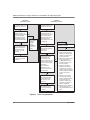
1
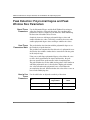
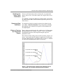
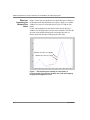
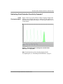
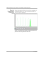
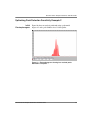
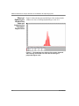
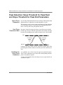
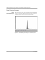
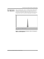
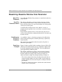
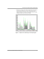
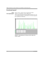
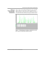
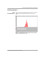
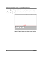
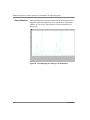
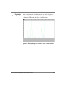
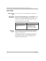
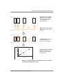
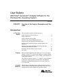
User Bulletin
ABI PRISM® GeneScan® Analysis Software for the
Windows NT® Operating System
June 2002
SUBJECT:
Overview of the Analysis Parameters and Size
Caller
Introduction
In This User
Bulletin
Purpose
This user bulletin includes the following topics:
GeneScan Analysis Software Process . . . . . . . . . . . . . . . . . . . . . . . . 2
Analysis Parameters . . . . . . . . . . . . . . . . . . . . . . . . . . . . . . . . . . . . . 3
Analysis Parameters Dialog Box. . . . . . . . . . . . . . . . . . . . . . . . . . . . 4
Data Processing: Smooth Options Parameter . . . . . . . . . . . . . . . . . . 5
Peak Detection: Min. Peak Half Width Parameter . . . . . . . . . . . . . . 7
Peak Detection: Polynomial Degree and Peak Window Size
Parameters . . . . . . . . . . . . . . . . . . . . . . . . . . . . . . . . . . . . . . . . . . . . . 8
Peak Detection: Slope Threshold for Peak Start and Slope
Threshold for Peak End Parameters . . . . . . . . . . . . . . . . . . . . . . . . 16
Baselining: Baseline Window Size Parameter . . . . . . . . . . . . . . . . 20
Size Caller . . . . . . . . . . . . . . . . . . . . . . . . . . . . . . . . . . . . . . . . . . . . 30
This user bulletin supplements the ABI PRISM® GeneScan Analysis
Software version 3.7 User Guide (P/N 4308923) to further explain
the analysis parameters and size caller available in the Windows NT®
version of the software.
The GeneScan Analysis Software v3.7.1 Updater CD (P/N 4336026)
includes new analysis parameter default values. For additional
information and installation instructions, refer to the GeneScan
v3.7.1 About file.
Intended
Audience
This document is intended for users familiar with the GeneScan
analysis software for the Macintosh® operating system who are now
using the software on the Windows NT operating system.
DRAFT
June 4, 2002 11:13 am, 4335617A.fm
ABI PRISM®GeneScan® Analysis Software for the Windows NT® Operating System
GeneScan Analysis Software Process
Overview
Flowchart
The ABI PRISM® GeneScan Analysis Software is available in versions
for both the Windows NT operating system and the Macintosh
operating system. The Windows NT version of the software uses
different algorithms and has additional analysis parameters that give
users more control with data analysis.
The following flowchart shows how GeneScan analysis software
analyzes data.
Note: For multicapillary instruments, multicomponenting is
performed by the data collection software.
Raw data
Limit
analysis range
No
Sizecalling
needed?
Yes
Multicomponent
Match
size standard
Baseline
Quality check
Detect peaks
Make
sizing curve
Smooth analyzed
electropherogram
Size peaks
Analyzed data
Figure 1 Simplified GeneScan analysis software flowchart
2
DRAFT
June 4, 2002 11:13 am, 4335617A.fm
User Bulletin
Overview of the Analysis Parameters and Size Caller
Analysis Parameters
Table of
Parameters
The following table lists the analysis parameters:
Parameter Status
Parameter
Discussed in...
Unchanged from
Macintosh versions
• Analysis Range
• Size Call Range
• Size Calling
Method
• Peak Amplitude
Thresholds
ABI PRISM® GeneScan
Analysis Software
Version 3.7 User
Guide
• Smooth Options
• Min. Peak Half
Width
this user bulletin and
the ABI PRISM®
GeneScan Analysis
Software Version
3.7 NT and 3.1
Macintosh User
Guides
• Polynomial Degree
• Peak Window Size
• Slope Threshold
for Peak Start
• Slope Threshold
for Peak End
• Window Size
this user bulletin and
the ABI PRISM®
GeneScan Analysis
Software Version 3.7
User Guide
Baseline
Multicomponent
ABI PRISM®
GeneScan Analysis
Software version 3.1
User’s Manual
Changed from
Macintosh versions
Added for the
Windows NT version
Removed options
from the Windows
NT version
Overview of the Analysis Parameters and Size Caller
DRAFT
June 4, 2002 11:13 am, 4335617A.fm
3
ABI PRISM®GeneScan® Analysis Software for the Windows NT® Operating System
Analysis Parameters Dialog Box
About the
Analysis
Parameters
Dialog Box
Example
Use the Analysis Parameters dialog box to set analysis parameter
values for data processing.
The default analysis parameter values are analysis guidelines. This
bulletin should serve as a guide for modifying these values as
appropriate for each laboratory.
Figure 2 shows the Analysis Parameters dialog box with default
values for GeneScan analysis software v3.7.1 on the Windows NT
operating system.
Figure 2
4
Analysis Parameters dialog box displaying default values
DRAFT
June 4, 2002 11:13 am, 4335617A.fm
User Bulletin
Overview of the Analysis Parameters and Size Caller
Data Processing: Smooth Options Parameter
About the
Parameter
The Smooth Options parameter sets the degree of smoothing applied
to the display of the analyzed electropherogram. Smoothing may aid
in data interpretation.
How the
Parameter Works
The Smooth Options parameter is applied after peak detection and
affects only the display of analyzed electropherograms. The peak
heights and areas are calculated and displayed in the tabular data
display based on the “none” smoothing option. Selecting light or
heavy smoothing will not affect the calculation of these values.
Smoothing
Example
Figure 3 shows the peaks from the same sample file after analysis
using no smoothing (black); light smoothing (green); and heavy
smoothing (red). All tabular data, including peak height and area,
remain unchanged.
No smoothing (black)
Light smoothing (green)
Heavy smoothing (red)
Figure 3 Electropherogram showing the effects of smoothing on
peaks from the same sample file
Overview of the Analysis Parameters and Size Caller
DRAFT
June 4, 2002 11:13 am, 4335617A.fm
5
ABI PRISM®GeneScan® Analysis Software for the Windows NT® Operating System
Figure 4 Electropherogram showing the effects of smoothing
on the smaller peak and baseline by changing the y scale
from Figure 3
6
DRAFT
June 4, 2002 11:13 am, 4335617A.fm
User Bulletin
Overview of the Analysis Parameters and Size Caller
Peak Detection: Min. Peak Half Width Parameter
About This
Parameter
Use the Min. Peak Half Width parameter to specify the smallest full
width at half maximum height for peak detection. This parameter can
be used to ignore noise spikes.
How This
Parameter Works
The Min. Peak Half Width parameter defines what constitutes a peak.
The software ignores peak half widths smaller than the specified
value.
The way in which this version of the software defines the minimum
peak half width is different than in previous versions.
Old Versions
Current Version
Half
height
Full
width
Half
width
Half width of the peak measured
from peak start
Full width of the peak measured at
half its height
Figure 5 Defining the Min. Peak Half Width
Overview of the Analysis Parameters and Size Caller
DRAFT
June 4, 2002 11:13 am, 4335617A.fm
7
ABI PRISM®GeneScan® Analysis Software for the Windows NT® Operating System
Peak Detection: Polynomial Degree and Peak
Window Size Parameters
About These
Parameters
Use the Polynomial Degree and the Peak Window Size settings to
adjust the sensitivity of the peak detection. You can adjust these
parameters to detect a single base pair difference while minimizing
the detection of shoulder effects or noise.
Sensitivity increases with larger polynomial degree values and
smaller window size values. Conversely, sensitivity decreases with
smaller polynomial degree values and larger window size values.
How These
Parameters Work
The peak window size functions with the polynomial degree to set
the sensitivity of peak detection.
The peak detector computes the first derivative of a polynomial curve
fitted to the data within a window that is centered on each data point
in the analysis range.
Using curves with larger polynomial degree values allows the curve
to more closely approximate the signal and, therefore, the peak
detector captures more peak structure in the electropherogram.
The peak window size sets the width (in data points) of the window to
which the polynomial curve is fitted to data. Higher peak window
size values smooth out the polynomial curve, which limits the
structure being detected. Smaller window size values allow a curve to
better fit the underlying data.
How to Use
These
Parameters
8
Use the table below to adjust the sensitivity of detection.
Polynomial
Degree Value
Window Size
Value
Increase sensitivity use...
Higher
Lower
Decrease sensitivity use...
Lower
Higher
To...
DRAFT
June 4, 2002 11:13 am, 4335617A.fm
User Bulletin
Overview of the Analysis Parameters and Size Caller
Guidelines for
Using These
Parameters
To detect well-isolated, base-line-resolved peaks, use polynomial
degree values of 2 or 3. For finer control, use a degree value of 4 or
greater.
As a guideline, set the peak window size (in data points) to be about 1
to 2 times the full width at half maximum height of the peaks that you
want to detect.
Examining Peak
Definitions
Effects of Varying
the Polynomial
Degree
To examine how GeneScan Analysis software has defined a peak,
select View > Show Peak Positions. The peak positions, including
the beginning, apex, and end of each peak, are tick-marked in the
electropherogram.
Figure 6 depicts peaks detected with a window size of 15 data points
and a polynomial curve of degree 2 (green); 3 (red); and 4 (black).
The diamonds represent a detected peak using the respective
polynomial curves.
Note that the smaller trailing peak is not detected using a degree of 2
(green). As the peak detection window is applied to each data point
across the displayed region, a polynomial curve of degree 2 could not
be fitted to the underlying data to detect its structure.
Polynomial curve of degree 4
(black)
Polynomial curve of degree 3
(red)
Polynomial curve of degree 2
(green)
Figure 6 Electropherogram showing peaks detected with the
same window size and three different polynomial degrees
Overview of the Analysis Parameters and Size Caller
DRAFT
June 4, 2002 11:13 am, 4335617A.fm
9
ABI PRISM®GeneScan® Analysis Software for the Windows NT® Operating System
Effects of
Increasing the
Window Size
Value
Figure 7 shows the same peaks that are shown in Figure 6. However,
in this depiction both polynomial curves have a degree of 3 and the
window size value was increased from 15 (red) to 31(black) data
points.
As the cubic polynomial is stretched to fit the data in the larger
window size, the polynomial curve becomes smoother. Note that the
structure of the smaller trailing peak is no longer detected as a
distinct peak from the adjacent larger peak to the right.
Window size value of 31 (black)
Window size value of 15 (red)
Figure 7 Electropherogram showing the same peaks as
in Figure 6 after increasing the window size value while keeping
the polynomial degree the same
10
DRAFT
June 4, 2002 11:13 am, 4335617A.fm
User Bulletin
Overview of the Analysis Parameters and Size Caller
Optimizing Peak Detection Sensitivity Example 1
Initial
Electropherogram
Figure 8 shows two resolved alleles of known fragment lengths (that
differ by one nucleotide) detected as a single peak. The analysis was
performed using a polynomial degree of 3 and a peak window size of
19 data points.
Figure 8 Electropherogram showing two resolved alleles
detected as a single peak
Note: For information on the tick marks displayed in the
electropherogram, see “Examining Peak Definitions” on page 9.
Overview of the Analysis Parameters and Size Caller
DRAFT
June 4, 2002 11:13 am, 4335617A.fm
11
ABI PRISM®GeneScan® Analysis Software for the Windows NT® Operating System
Effects of
Decreasing the
Window Size
Value
Figure 9 shows that both alleles are detected after re-analyzing with
the polynomial degree set to 3 while decreasing the window size
value to 15 (from 19) data points.
Figure 9 Electropherogram showing the alleles detected as two
peaks after decreasing the window size value
12
DRAFT
June 4, 2002 11:13 am, 4335617A.fm
User Bulletin
Overview of the Analysis Parameters and Size Caller
Optimizing Peak Detection Sensitivity Example 2
Initial
Electropherogram
Figure 10 shows an analysis performed using a polynomial
degree of 3 and a peak window size of 19 data points.
Figure 10 Electropherogram showing four resolved peaks
detected as two peaks
Overview of the Analysis Parameters and Size Caller
DRAFT
June 4, 2002 11:13 am, 4335617A.fm
13
ABI PRISM®GeneScan® Analysis Software for the Windows NT® Operating System
Effects of
Reducing the
Window Size
Value and
Increasing the
Polynomial
Degree Value
Figure 11 shows the data presented in Figure 10 re-analyzed with a
window size value of 10 and polynomial degree value of 5.
Figure 11 Electropherogram showing all four peaks detected
after reducing the window size value and increasing the
polynomial degree value
14
DRAFT
June 4, 2002 11:13 am, 4335617A.fm
User Bulletin
Overview of the Analysis Parameters and Size Caller
Optimizing Peak Detection Sensitivity Example 3
Effects of
Extreme Settings
Figure 12 shows the result of an analysis using a peak window size
value set to 10 and a polynomial degree set to 9. This extreme setting
for peak detection led to several peaks being split and detected as two
separate peaks.
Figure 12 Electropherogram showing the result of an analysis
using extreme settings for peak detection
Overview of the Analysis Parameters and Size Caller
DRAFT
June 4, 2002 11:13 am, 4335617A.fm
15
ABI PRISM®GeneScan® Analysis Software for the Windows NT® Operating System
Peak Detection: Slope Threshold for Peak Start
and Slope Threshold for Peak End Parameters
About These
Parameters
Use the Slope Threshold for Peak Start and Slope Threshold for Peak
End parameters to adjust the start and end points of a peak.
This parameter can be used to better position the start and end points
of an asymmetrical peak, or a poorly resolved shouldering peak, to
more accurately reflect the peak position and area.
How These
Parameters Work
In general, from left to right, the slope of a peak increases from the
baseline up to the apex. From the apex down to the baseline, the slope
becomes decreasingly negative until it returns to zero at the baseline.
Apex
Increasingly
positive
slope
(+)
Baseline
0
Increasingly
negative
slope
(–)
0
If either of the slope values you have entered exceeds the slope of the
peak being detected, the software overrides your value and reverts to
zero.
Guidelines for
Using These
Parameters
As a guideline, use a value of zero for typical or symmetrical peaks.
Select values other than zero to better reflect the beginning and end
points of asymmetrical peaks.
A value of zero will not affect the sizing accuracy or precision for an
asymmetrical peak.
16
DRAFT
June 4, 2002 11:13 am, 4335617A.fm
User Bulletin
Overview of the Analysis Parameters and Size Caller
Using These
Parameters
Use the table below to move the start or end point of a peak.
IF you want to move the...
THEN change the...
start point of a peak
closer to its apex
Slope Threshold for Peak Start value
from zero to a positive number
end point of a peak
closer to its apex
Slope Threshold for Peak End value
to an increasingly negative number
Note: The size of a detected peak is the calculated apex between the
start and end points of a peak and will not change based on your
settings.
Overview of the Analysis Parameters and Size Caller
DRAFT
June 4, 2002 11:13 am, 4335617A.fm
17
ABI PRISM®GeneScan® Analysis Software for the Windows NT® Operating System
Slope Threshold Example
Initial
Electropherogram
The initial analysis with a value of 0 for both the Slope Threshold for
Peak Start and the Slope Threshold for Peak End value produced an
asymmetrical peak with a noticeable tail on the right side.
Figure 13
18
Electropherogram showing an asymmetrical peak
DRAFT
June 4, 2002 11:13 am, 4335617A.fm
User Bulletin
Overview of the Analysis Parameters and Size Caller
Electropherogram
After Adjustments
After re-analyzing with a value of –35.0 for the Slope Threshold for
Peak End, the end point that defines the peak moves closer to its
apex, thereby removing the tailing feature. Note that the only change
to tabular data was the area (peak size and height are unchanged).
.
Figure 14 Electropherogram showing the effect of changing the
slope threshold for peak end
Overview of the Analysis Parameters and Size Caller
DRAFT
June 4, 2002 11:13 am, 4335617A.fm
19
ABI PRISM®GeneScan® Analysis Software for the Windows NT® Operating System
Baselining: Baseline Window Size Parameter
About This
Parameter
Use the Baseline Window Size parameter to control the baseline for a
group of peaks.
How This
Parameter Works
The software determines a reference baseline value for each data
point. In general, the software sets the reference baseline to be the
lowest value that it detects in a specified window size (in data points)
centered on each data point.
A small baseline window relative to the width of a cluster, or
grouping of peaks spatially close to each other, can result in shorter
peak heights.
Larger baseline windows relative to the peaks being detected can
create an elevated baseline, resulting in peaks that are elevated or not
baseline resolved.
Guidelines for
Using This
Parameter
As a guideline, choose a value that encompasses the width in data
points of the peaks being detected while preserving a qualitatively
smooth baseline.
The trade-off for a smoother baseline that touches all peaks is a
reduction in peak height.
Baselining
Example
Figure 15 depicts an allelic ladder containing clusters of alleles. The
alleles have been labeled with green dye and the data displayed has
been multicomponented, but not baselined. The electropherogram
spans approximately 2800 data points.
The red, blue, and black traces depict various reference baselines
(zero in the analyzed electropherogram) that result from different
baseline window size settings. These reference baselines are
subtracted from the sample data during baselining. In Figure 15:
• The red trace depicts the reference baseline that results from an
extreme baseline window size value of 2801. At this setting, the
reference baseline does not touch all peaks, resulting in elevated
peak heights.
• The blue trace depicts the reference baseline that results from the
default value of 51 data points.
20
DRAFT
June 4, 2002 11:13 am, 4335617A.fm
User Bulletin
Overview of the Analysis Parameters and Size Caller
• The black trace depicts the reference baseline that results from an
extreme baseline window size value of 5 data points. At this
setting, the peaks are tracked too closely by the reference baseline,
resulting in significantly reduced peak height.
Figure 15
Depiction of the baselining of an electropherogram
Overview of the Analysis Parameters and Size Caller
DRAFT
June 4, 2002 11:13 am, 4335617A.fm
21
ABI PRISM®GeneScan® Analysis Software for the Windows NT® Operating System
Baselining Example 1
Initial
Electropherogram
Figure 16 shows a portion of the electropherogram shown
in Figure 15, which depicts various window sizes.
The electropherogram shows the default Baseline Window Size value
of 51 that appears in Figure 15 as the blue trace. Note that all peaks in
this cluster have been baselined.
Figure 16 Electropherogram showing an allelic ladder with a
cluster of peaks
22
DRAFT
June 4, 2002 11:13 am, 4335617A.fm
User Bulletin
Overview of the Analysis Parameters and Size Caller
Effects of
Extreme Increase
of the Baseline
Window Size
Figure 17 shows an extreme Baseline Window Size value of 2801 that
appears in Figure 15 as the red trace. (2801 is approximately the
width in data points of all the peaks shown.) This increase resulted in
an overall raised baseline and many elevated peaks within the cluster.
Figure 17 Electropherogram showing a raised baseline caused
by an increase in the baseline window size value
Overview of the Analysis Parameters and Size Caller
DRAFT
June 4, 2002 11:13 am, 4335617A.fm
23
ABI PRISM®GeneScan® Analysis Software for the Windows NT® Operating System
Effects of
Extreme
Decrease of the
Baseline Window
Size
Figure 18 shows an extreme Baseline Window Size value of 5 that
appears in Figure 15 as the black trace. (Five is much smaller than the
width in data points for any of the peaks prior to baselining.) This
decrease resulted in a significant decrease in the peak heights.
Figure 18 Electropherogram showing significantly reduced peak
heights caused by a reduction in the baseline window size value
24
DRAFT
June 4, 2002 11:13 am, 4335617A.fm
User Bulletin
Overview of the Analysis Parameters and Size Caller
Baselining Example 2
Initial
Electropherogram
Figure 19 shows the electropherogram from an analysis of a cluster of
peaks using the default Baseline Window Size value of 51 data
points.
Figure 19 Electropherogram showing a typical result using the
default baseline window size value
Overview of the Analysis Parameters and Size Caller
DRAFT
June 4, 2002 11:13 am, 4335617A.fm
25
ABI PRISM®GeneScan® Analysis Software for the Windows NT® Operating System
Effects of
Extreme
Decrease of the
Baseline Window
Size
Figure 20 shows the re-analysis of the electropherogram shown in
Figure 19 with an extreme Baseline Window Size value of 5. All
peaks within the cluster have been baselined and have a reduced peak
height.
Figure 20 Electropherogram showing dramatically reduced peak
heights caused by a reduction in the baseline window size value
26
DRAFT
June 4, 2002 11:13 am, 4335617A.fm
User Bulletin
Overview of the Analysis Parameters and Size Caller
Baselining Example 3
Raw Data
The data in the electropherogram has been multicomponented but not
baselined. There are two pull-down peaks in the blue trace below the
two major green peaks (see arrows).
Figure 21 Electropherogram showing raw data that has been
multicomponented but not baselined
Overview of the Analysis Parameters and Size Caller
DRAFT
June 4, 2002 11:13 am, 4335617A.fm
27
ABI PRISM®GeneScan® Analysis Software for the Windows NT® Operating System
Raised Baseline
After analyzing with a baseline window size of 251 data points, the
low points represented in the blue trace (within this 251 data point
window) are set to zero. This results in a raised baseline between
these points.
Figure 22
28
Electropherogram showing a raised baseline
DRAFT
June 4, 2002 11:13 am, 4335617A.fm
User Bulletin
Overview of the Analysis Parameters and Size Caller
Eliminating
Raised Baseline
After re-analyzing with a baseline window size of 51 data points (a
window size range between the pull-down peaks), the raised baseline
is eliminated. This results in a more accurate baseline.
Figure 23
Electropherogram showing a more accurate baseline
Overview of the Analysis Parameters and Size Caller
DRAFT
June 4, 2002 11:13 am, 4335617A.fm
29
ABI PRISM®GeneScan® Analysis Software for the Windows NT® Operating System
Size Caller
About the Size
Caller
How the Size
Caller Works
The size caller matches size-standard peaks with a quality check.
The way in which the fragment sizes are calculated has not changed
from previous versions of the software (e.g., local southern).
However, the way in which the Windows NT version of the software
identifies the size standard is different from previous versions.
Method for Identifying the Size Standard
Macintosh
Version
Macintosh Versions
Windows NT Version
User assigns fragment sizes to
particular peaks based on scan
number
Software matches the size
standard fragments by ratio
matching based on relative
distance between neighboring
peaks
In GeneScan analysis software for the Macintosh operating system,
the size standard peaks are identified based on their assignment
within a run or a previous run.
Anomalous peaks outside of a ±10 data point bin are ignored, but
those within the bins can be incorrectly called resulting in an
incorrect size curve. In that case, you must redefine a new size
standard for that particular sample.
30
DRAFT
June 4, 2002 11:13 am, 4335617A.fm
User Bulletin
Overview of the Analysis Parameters and Size Caller
Base Pair
50
100
Data Point 100
200
Base Pair
100
50
200
Defining the Size Standard
The boxes show a ±10 data
point range used to identify
size standard peaks in
subsequent runs
400
400
800
200
Data (100, 200, 400, and 800)
shown with anomalous peak
dotted
400
Assigning Peaks that fall into
the correct range. The
anomalous peak is ignored.
Data Point 100
200
400
800
500
Generating the Size Standard
Curve for sample file using
specified sizing method, e.g.,
Local Southern
Base pair
400
300
200
100
0
0
100 200 300 400 500 600 700 800 900
Data point
Figure 24 Peak identification with GeneScan analysis software
for the Macintosh operating system
Overview of the Analysis Parameters and Size Caller
DRAFT
June 4, 2002 11:13 am, 4335617A.fm
31
ABI PRISM®GeneScan® Analysis Software for the Windows NT® Operating System
Windows NT
Version
GeneScan analysis software for the Windows NT operating system
uses ratio matching to identify the size standard fragments.
Ratio matching does not rely on the manual assignment of size
standard definitions (in base pairs) to their associated data points
within a run or a previous run. Selecting a peak in the
electropherogram to enter an associated value in the Size column now
serves only as a guide. Simply listing the values to be used for sizing
as an array of numbers without regard to the highlighted peak is
sufficient.
Figure 25 Electropherogram showing a selected peak and the
associated value in the Size column
The size caller ignores anomalous peaks that do not match the
expected ratio. The size caller constructs a best-fit curve using the
data points of each size standard fragment detected. A comparison
between the sizes calculated from the best-fit curve and the matched
peaks from the size standard definition using the array of numbers is
performed. Size calling will fail if significant differences are found
or if no match can be made based on the expected ratios. (In Figure
26, that is x, 2x, and 4x.) Additionally, you may find that one of the
size fragments has not been identified, even though it was listed as
part of the definition. The size caller has been designed to allow the
exclusion of one of the listed values to obtain a better match. To use
an excluded fragment, try the steps outlined in Figure 27.
32
DRAFT
June 4, 2002 11:13 am, 4335617A.fm
User Bulletin
Overview of the Analysis Parameters and Size Caller
Base pair
50
100
x
Scan # 100
Base
pair
50
100
x
Data
100
point
200
200
4x
400
800
Base
pair
50
100
x
4x
400
800
Defining the
Size Standard
from a list of
sizes (50, 100,
200, and 400)
used to
calculate the
expected ratios
(in red)
400
2x
400
2x
200
200
Data
100
point
200
2x
200
400
less than
4x
400
800
Data (100, 200,
400, and 800)
shown with
anomalous
peak dotted
Assigning
Peaks that
match the
expected ratio.
The anomalous
peak is ignored
500
Generating the
Size Standard
Curve when a
good ratio
match is found
Base pair
400
300
200
100
0
0
100 200 300 400 500 600 700 800 900
Data point
Figure 26 Peak identification with GeneScan analysis software
for the Windows NT operating system
Overview of the Analysis Parameters and Size Caller
DRAFT
June 4, 2002 11:13 am, 4335617A.fm
33
ABI PRISM®GeneScan® Analysis Software for the Windows NT® Operating System
GeneScan
Macintosh version
GeneScan
Windows NT version
All peaks present in size
standard are detected.
All peaks present in size
standard are detected.
Information in the size
standard definition is
used to select the peaks
of the size standard
(±10 data points from
the position defined in
the Size Standard file).
Information in the size
standard definition is
used to select the peaks
of the size standard
(ratio matching is used
based on the list of
sizes defined in the Size
Standard file).
Pass
Size standard curve is
constructed using the
method selected by
the user (e.g., local
southern).
Fail
New standard
for failed
sample is
defined,
regardless of
migration or
quality.
Sample is not sized.
Best fit curve of the
detected sized standard
fragments is
constructed.
For each peak in the
size standard, the
matched size of the
peak is compared to the
calculated size using the
best fit curve previously
constructed.
Size standard curve
used to size all peaks
in sample.
If the sizes differ
significantly or the
peaks cannot be found,
the sizing fails.
Pass
Size standard curve is
constructed using the
method selected by
the user (e.g., local
southern).
Size standard curve
used to size all peaks
in sample.
Figure 27
34
The user should:
1. Make sure all fragments
listed in the size standard
definition are reflected in
the analysis range.
Fail
2. Make sure the primer peak
is not interfering with
smaller fragments. If it is,
exclude the primer peak
from the analysis.
3. Make sure the higher
fragments are resolved.
If they are not, reduce the
analysis range and change
the size standard definition
to reflect the missing
peaks.
4. Attempt to get a better
ratio match by changing
the size standard definition
and analysis range to
analyze a smaller range
containing only peaks of
interest, if plausible.
5. Attempt to guess values for
any split peaks so that
every peak displayed has a
value.
Peak sizing flowcharts
DRAFT
June 4, 2002 11:13 am, 4335617A.fm
User Bulletin
Overview of the Analysis Parameters and Size Caller
Overview of the Analysis Parameters and Size Caller
DRAFT
June 4, 2002 11:13 am, 4335617A.fm
35
© Copyright 2002, Applied Biosystems. All rights reserved.
For Research Use Only. Not for use in diagnostic procedures.
Information in this document is subject to change without notice. Applied
Biosystems assumes no responsibility for any errors that may appear in this
document. This document is believed to be complete and accurate at the
time of publication. In no event shall Applied Biosystems be liable for
incidental, special, multiple, or consequential damages in connection with or
arising from the use of this document.
Applied Biosystems, ABI PRISM and its design, and GeneScan are registered
trademarks and AB (Design) and Applera are trademarks of
Applera Corporation or its subsidiaries in the U.S. and certain other countries.
Microsoft, Windows, and Windows NT are registered trademarks of Microsoft
Corporation.
Macintosh is a registered trademarks of Apple Computer, Inc.
Headquarters
850 Lincoln Centre Drive
Foster City, CA 94404 USA
Phone: +1 650.638.5800
Toll Free (In North America): +1 800.345.5224
Fax: +1 650.638.5884
Worldwide Sales and Support
Applied Biosystems vast distribution and
service network, composed of highly trained
support and applications personnel, reaches
into 150 countries on six continents. For sales
office locations and technical support, please
call our local office or refer to our web site at
www. applied biosystems.com.
All other trademarks are the sole property of their respective owners.
www.appliedbiosystems.com
Applera Corporation is committed to providing the
world’s leading technology and information for life
scientists. Applera Corporation consists of the
Applied Biosystems and Celera Genomics
businesses.
Printed in USA, 06/2002
Part Number 4335617 Rev. A, Stock Number 106UB35-01